by Jason Robert King - University of Toronto
83
Quadrotor Visual Servoing for Automatic Landing by Jason Robert King A thesis submitted in conformity with the requirements for the degree of Master of Applied Science University of Toronto Institute for Aerospace Studies University of Toronto c Copyright 2017 by Jason Robert King
Transcript of by Jason Robert King - University of Toronto

Quadrotor Visual Servoing for Automatic Landing
by
Jason Robert King
A thesis submitted in conformity with the requirementsfor the degree of Master of Applied Science
University of Toronto Institute for Aerospace StudiesUniversity of Toronto
c© Copyright 2017 by Jason Robert King

Abstract
Quadrotor Visual Servoing for Automatic Landing
Jason Robert King
Master of Applied Science
University of Toronto Institute for Aerospace Studies
University of Toronto
2017
This thesis investigates the application of camera-based tracking and landing for multi-
rotor UAVs on a moving target. Both Position-Based and Image-Based Visual Servoing
are utilized to provide guidance to the quadrotor which will aim to track the target and
to land on top of it. A novel Image-Based Visual Servoing scheme with a non-static
desired image is developed to facilitate landing and yawing motions by the quadrotor.
These control laws are then investigated through simulation and implementation on an
experimental platform.
Experiments are performed using the Ardrone 2.0 quadrotor and a Create Roomba
as the ground rover. Successful implementations for landing are presented in the case of
the Position-Based Visual Servoing, while hover and small motions are performed using
the Image-Based Visual Servoing.
ii

Acknowledgements
First and foremost my sincere thanks go to Professor Liu for his support, mentorship
and guidance throughout this project. His door was always open for the smallest or the
largest problems.
I’d like to thank the members of my Research Assessment Committee, Prof. C. J.
Damaren and Prof. P. R. Grant, for their feedback and guidance during this project.
I’d also like to thank my labmates and classmates for helpful discussions and comments,
both in one-on-one discussions and particularly during our weekly group meetings. At
the risk of forgetting someone, I would like to specifically thank Henry Zhu, Samuel Zhao,
and Quinrui Zhang.
Finally I’d like to thank my family, who were always there to lend a helping hand
when needed, both throughout this Masters and throughout my life. This work would
not have been possible without them.
iii
Contents
Acknowledgements iii
Contents iv
List of Tables vi
List of Figures vii
1 Introduction 1
1.1 Literature Review . . . . . . . . . . . . . . . . . . . . . . . . . . . . . . . 2
1.1.1 Visual Servoing . . . . . . . . . . . . . . . . . . . . . . . . . . . . 2
1.1.2 Quadrotor Control: . . . . . . . . . . . . . . . . . . . . . . . . . . 6
1.1.3 Visual Servoing applied to UAV landing . . . . . . . . . . . . . . 6
2 Quadrotor Model and Control 10
2.1 Reference frames . . . . . . . . . . . . . . . . . . . . . . . . . . . . . . . 10
2.2 Quadrotor Model and Dynamics . . . . . . . . . . . . . . . . . . . . . . . 12
2.3 Equations of Motion and Linearization . . . . . . . . . . . . . . . . . . . 14
2.4 Summary . . . . . . . . . . . . . . . . . . . . . . . . . . . . . . . . . . . 17
3 Image Based Visual Servoing 18
3.1 Classical Image-Based Visual Servoing . . . . . . . . . . . . . . . . . . . 18
3.1.1 IBVS Control Law Design . . . . . . . . . . . . . . . . . . . . . . 21
3.1.2 IBVS Control Law Architecture . . . . . . . . . . . . . . . . . . . 22
3.2 Virtual Camera IBVS . . . . . . . . . . . . . . . . . . . . . . . . . . . . . 23
3.3 IBVS with Non-Static Desired Image . . . . . . . . . . . . . . . . . . . . 26
3.3.1 Proof of stability for moving desired image . . . . . . . . . . . . . 27
3.4 Landing strategies and applications to image-based approaches . . . . . . 31
3.4.1 Approaches to landing maneuvers . . . . . . . . . . . . . . . . . . 31
iv

3.4.2 Image-Based landings . . . . . . . . . . . . . . . . . . . . . . . . . 32
3.5 Simulations work . . . . . . . . . . . . . . . . . . . . . . . . . . . . . . . 33
3.5.1 Classical and Virtual IBVS . . . . . . . . . . . . . . . . . . . . . . 34
3.5.2 Virtual and Non-Static Virtual IBVS . . . . . . . . . . . . . . . . 35
3.5.3 Landing using non-static target images . . . . . . . . . . . . . . . 37
3.6 Summary . . . . . . . . . . . . . . . . . . . . . . . . . . . . . . . . . . . 38
4 Position Based Visual Servoing 39
4.1 Architecture of standard PBVS controls . . . . . . . . . . . . . . . . . . 39
4.1.1 Simulations with time delays . . . . . . . . . . . . . . . . . . . . . 42
4.2 Stability proof for constant yawing rate target . . . . . . . . . . . . . . . 43
4.3 Simulations Work . . . . . . . . . . . . . . . . . . . . . . . . . . . . . . . 44
4.3.1 Yaw simulations . . . . . . . . . . . . . . . . . . . . . . . . . . . . 44
4.4 Saturated total velocity controller . . . . . . . . . . . . . . . . . . . . . . 44
4.5 Simplified PBVS - S-PBVS . . . . . . . . . . . . . . . . . . . . . . . . . . 47
4.6 Summary . . . . . . . . . . . . . . . . . . . . . . . . . . . . . . . . . . . 48
5 Experimental Setup 49
5.1 Optitrack . . . . . . . . . . . . . . . . . . . . . . . . . . . . . . . . . . . 49
5.2 Ground rover - the Create Roomba . . . . . . . . . . . . . . . . . . . . . 50
5.3 Flying Platform 1: Ardrone 2.0 quadcopter . . . . . . . . . . . . . . . . . 51
5.3.1 PBVS design for Ardrone . . . . . . . . . . . . . . . . . . . . . . 54
5.3.2 IBVS design . . . . . . . . . . . . . . . . . . . . . . . . . . . . . . 57
5.4 Summary . . . . . . . . . . . . . . . . . . . . . . . . . . . . . . . . . . . 60
6 Experimental Results 61
6.1 Optitrack setup . . . . . . . . . . . . . . . . . . . . . . . . . . . . . . . . 61
6.2 ArDrone 2.0 PBVS Results: . . . . . . . . . . . . . . . . . . . . . . . . . 62
6.2.1 PBVS without Optitrack information . . . . . . . . . . . . . . . . 62
6.2.2 PBVS with Optitrack information . . . . . . . . . . . . . . . . . . 63
6.3 IBVS with ArDrone . . . . . . . . . . . . . . . . . . . . . . . . . . . . . . 67
6.3.1 Non-Static-IBVS compared with Classical IBVS . . . . . . . . . . 68
6.4 Summary . . . . . . . . . . . . . . . . . . . . . . . . . . . . . . . . . . . 69
7 Conclusions 70
Bibliography 72
v
List of Tables
3.1 Ardrone physical properties . . . . . . . . . . . . . . . . . . . . . . . . . 33
3.2 PID controller gains . . . . . . . . . . . . . . . . . . . . . . . . . . . . . 34
vi

List of Figures
1.1 Rendering of project objective . . . . . . . . . . . . . . . . . . . . . . . . 9
2.1 Reference frames utilized in this thesis . . . . . . . . . . . . . . . . . . . 11
2.2 Pinhole Camera Model . . . . . . . . . . . . . . . . . . . . . . . . . . . . 11
2.3 Quadrotor Model . . . . . . . . . . . . . . . . . . . . . . . . . . . . . . . 13
3.1 Relative Orientation of reference frames . . . . . . . . . . . . . . . . . . . 19
3.2 Quadrotor IBVS control architecture . . . . . . . . . . . . . . . . . . . . 22
3.3 Virtual Camera motivation . . . . . . . . . . . . . . . . . . . . . . . . . . 24
3.4 Cartesian position of quadrotor with Classic IBVS and Virtual IBVS. . . 35
3.5 Angular motion of quadrotor with Classic IBVS and Virtual IBVS. . . . 35
3.6 Yawing motion of a quadrotor with VIBVS and a Non-Static desired image
VIBVS. . . . . . . . . . . . . . . . . . . . . . . . . . . . . . . . . . . . . 36
3.7 Landing of a quadrotor using IBVS with non-static desired image. . . . . 37
4.1 PBVS Architecture . . . . . . . . . . . . . . . . . . . . . . . . . . . . . . 40
4.2 Tracking performance of all three controllers for stationary, constant ve-
locity and circular motion targets (single axis). . . . . . . . . . . . . . . . 41
4.3 Pitch angle or Error measured for the simulations in 4.2. . . . . . . . . . 41
4.4 Tracking performance and error for all three controllers - target performing
circular motion, with information delayed by 0.4 seconds. . . . . . . . . . 43
4.5 Yaw tracking performance for the Control Laws in Equations 4.5 . . . . . 45
4.6 Tracking performance for input saturated versus non saturated controllers. 46
4.7 Angle for input saturated versus non saturated controllers . . . . . . . . 46
5.1 Roomba ground rover with target taped on top . . . . . . . . . . . . . . 50
5.2 Ardrone 2.0 . . . . . . . . . . . . . . . . . . . . . . . . . . . . . . . . . . 51
5.3 Ardrone velocity readings when held immobile . . . . . . . . . . . . . . . 52
5.4 Experiment to determine the use of Optical flow in flight. . . . . . . . . . 53
5.5 Examples of performance of onboard tag detection . . . . . . . . . . . . . 54
vii

5.6 Ardrone control architecture . . . . . . . . . . . . . . . . . . . . . . . . . 55
5.7 Improved ArDrone architecture . . . . . . . . . . . . . . . . . . . . . . . 56
5.8 Yaw rectification algorithm number 1 . . . . . . . . . . . . . . . . . . . . 58
5.9 Ardrone IBVS Architecture . . . . . . . . . . . . . . . . . . . . . . . . . 59
6.1 Ardrone tracking a setpoint of (x=0,y=0,z=0.5) for different gains under
OptiTrack control. . . . . . . . . . . . . . . . . . . . . . . . . . . . . . . 62
6.2 Ardrone PBVS without Optitrack addition . . . . . . . . . . . . . . . . . 63
6.3 Position estimation by static Ardrone. . . . . . . . . . . . . . . . . . . . 64
6.4 Hover and position estimation by Ardrone over static target. . . . . . . . 64
6.5 Optitrack landing on a static target. . . . . . . . . . . . . . . . . . . . . 65
6.6 Optitrack landing on a slowly moving target - with no motion compensa-
tion term. . . . . . . . . . . . . . . . . . . . . . . . . . . . . . . . . . . . 65
6.7 Ardrone tracking a faster target - with motion compensation term. . . . 66
6.8 Optitrack landing on a quickly moving target - with motion compensation
term. . . . . . . . . . . . . . . . . . . . . . . . . . . . . . . . . . . . . . . 66
6.9 Ardrone under IBVS control . . . . . . . . . . . . . . . . . . . . . . . . . 67
6.10 Ardrone under IBVS control for yaw and height, optitrack control for
lateral position . . . . . . . . . . . . . . . . . . . . . . . . . . . . . . . . 68
viii

Chapter 1
Introduction
Unmanned Aerial Vehicles (UAVs) reduce aviation risks by removing the crew to a safe
location. They are less costly and easier to deploy than manned aircraft, as they do not
require the infrastructure or volatile fuels associated with manned aircraft.
In the past decade, the commercial use of UAVs has experienced exponential growth.
Initially confined to the military or research labs, the decrease in sensor and processing
costs as well as the maturity of autopilot technology have made these platforms easily
available. With the advent of low-cost UAVs the sky is much more accessible than it
used to be. This has led to a surge in activity in the UAV sector with applications as
diverse as Search and Rescue, mapping, and package delivery.
UAVs have already found widespread use, but they suffer from two major limitations.
The first is that most quadrotor UAVs operate outdoors and rely on operator observation
or GPS in addition to other onboard sensors for position control and navigation. The
restriction of good GPS signal limits the wide and reliable use of quadrotors, and is one
of the challenges that researchers are currently seeking to address. In order to reduce
dependence on GPS, much research in recent years has focused on using the camera as an
additional sensor for localization. The second drawback is that UAVs have short flight
times, which limits their operational range. A potential solution to this is to have the
UAV land and recharge on a mobile ground robot. This research seeks to address both
of these issues by using the camera to landing with respect to a visual target onboard
the mobile rover.
The reasons for using the camera are twofold. One is that cameras can be lightweight,
cheap and versatile. The second is that many UAVs already incorporate cameras for their
primary mission, making their use possible as an alternative navigation aid by processing
visual data.
The concept of using a vision sensor to localize or position a robot has been around
1

Chapter 1. Introduction 2
for several decades. Of the techniques that can be utilized to process the visual data,
simultaneous localization and mapping (SLAM) and optical flow are popular in research
and commercial use. This thesis investigates Visual Servoing, which makes use of prior
knowledge of the environment to localize using image data.
1.1 Literature Review
1.1.1 Visual Servoing
The concept of Visual Servoing originated in the 1980s, with the first review paper
published by Hutchinson, et al. in the mid 1990s [17]. A core group of researchers
including Chaumette, Hutchinson, Corke, Mahon and others led many of the initial
advances and remain active in the field to this day.
Visual Servoing is defined as using the camera to position a robot in a desired position
relative to an object. That is to say that a camera acquires images containing visual
features, which are then used to position the robot in a manner desired by the user
relative to those features. Visual Servoing systems can be classified into two groups
depending on where the camera is located [6].
One configuration is to have the cameras be located in the workspace pointed towards
the robot, known as “fixed in the workplace” configuration. In this configuration the im-
age provided is independent of the robot motion [6]. This configuration is commonly used
in motion capture systems such as OptiTrackTM or ViconTM - providing high accuracy
measurements of position and velocity to robots in laboratory settings. This configura-
tion is useful if there are many robots operating in a limited space as it requires more
setup but is then easier to control.
The second configuration is called “eye in hand”. As its name implies, it is where
a camera is mounted to the robot end-effector which is then servoed by using visual
cues. In this case, the robot motion affects the image, but the servoing can typically be
effected over larger distances and there is no need for external cameras. On the whole,
this configuration is more versatile and less costly (as a single camera can be used for a
larger space) but more complex due to the ego-motion of the camera with UAV motion.
Visual Servoing is further split into two broad categories - Position Based Visual
Servoing (PBVS) and Image Based Visual Servoing (IBVS). They differ in terms of the
utilization of the image features in the control law [24]. In PBVS, the image features are
utilized to calculate a relative position between the camera and a target. This relative
position between camera and target is then compared to the desired difference in position

Chapter 1. Introduction 3
and a control law is implemented. This control law should push the system to attain and
track the desired relative pose, or position and orientation. Because of the requirement
for estimation of relative pose, an object with a-priori known shape and dimensions is
required in the use of a PBVS control law [6].
IBVS, in contrast, maintains the error definition in the image space: it does not
explicitly calculate a relative position. Image features are detected in the image and
compared to the desired features. The difference between these two enables the control
law to calculate a desired velocity. Because there is no explicit recalculation of relative
pose it can be a computationally effective algorithm.
PBVS has two major advantages. The first is that it separates the control problem
from the error estimation and computation [27]. By calculating a relative position and
then controlling that position, one has a standard control design problem. Indeed, reg-
ulation of position is one of the basic control problems and there are many studies on
how to implement various control architectures or mechanisms. The second advantage
is that PBVS is globally stable [6]. The disadvantage is that because PBVS requires a
reconstruction of position, it requires more information about the object and relies more
heavily on an accurately calibrated camera [6]. In addition, because the control of the
robot does not necessarily take into account the camera image, visual features can easily
leave the Field of View (FOV) in a system controlled by PBVS.
Image-Based Visual Servoing does not rely as much on camera calibration or accurate
target information. Its disadvantage is that it is only locally stable and the region of
stability is ill-defined - this area is a potential area for further research. The most
information that this review found in the literature is the “neighbourhood is surprisingly
quite large in practice” [6]. Classical IBVS requires only a few points on the image, their
desired position on the image, and an approximate depth to those points. In particular
for the moving UAV case, one problem was the coupling between the error and the aircraft
dynamics which makes control laws difficult to design. It also exhibits poor motion for
certain types of control inputs - notably yaw, which causes motion along the camera axis
[6]. Another difficulty is that IBVS is a velocity controller, which therefore requires at
least an approximation of the velocity of the system for control [39].
Multiple methods have been devised to attempt to reduce the disadvantages of IBVS.
First, attempts were made to find features that may exhibit gentle or conventional char-
acteristics and be decoupled from one another (e.g. points, lines, or spheres [10]). This
was not successful, as each feature had some undesirable characteristics. Secondly, sev-
eral researchers have tried to combine the advantageous features of IBVS and PBVS into
hybrid methods. These included 2 1/2D visual servoing [21], where the control problem

Chapter 1. Introduction 4
was decoupled according to translational and rotational elements which were evaluated
separately by homography (IBVS) and PBVS methodologies. The disadvantage of this
approach was sensitivity to noise, as well as the requirement to use at minimum 8 points
to reconstruct the homography. Another technique utilized was to try to decouple mo-
tions around the various axes - typically separating the Z axis because it is the least
sensitive to motion. These efforts continue to this day, with some recent works, including
those by Zhao et al. [38], who utilize two neural network-image features to try to improve
conditioning of the image jacobian for the rotational X and Y axes - only a problem for
IBVS with a 6-DOF robot. This recent paper and many others have utilized various
image features and their interaction matrices described in Chaumette et al.’s 2004 paper
[5]. These authors highlighted image moments which have been subsequently exploited
by other researchers [11, 13, 24, 37].
More recently many techniques have been designed with additional complexity that
enable better performance from IBVS, particularly from underactuated systems. These
include state transition approaches such as those by Fink et al. in [11], where the dynam-
ics of the UAV are taken into account along with the use of novel image features from
Chaumette’s 2004 paper [5]. Although this controller works well to stabilize the lateral
dynamics it does not control the altitude of the quadrotor, which as a result drops over
the course of the experiment.
Implementing IBVS algorithms on quadrotors poses an additional problem due to
the underactuated property of quadrotors. Underactuated platforms such as quadrotors
led researchers to develop means of attempting to remove the roll/pitch coupling with
the image error. These are typically referred to as Dynamic IBVS techniques, because
they take into account the dynamics of the experimental platform. There are four main
methods in the literature:
• using spherical projection image points [14] - treating all points as though they
were on a unit sphere, and then de-rotating to keep them facing straight down;
• using a virtual spring approach [24] - using standard IBVS on yaw and height
channels, adding a compensation term related to the roll and pitch angles such
that the increase in image error due to pitch and roll does not lead to further
control inputs;
• using homography projection [26]. A homography matrix embeds information re-
garding the transformation between two images. In this case the selected two
images are the desired view of the target and the current view - this is then utilized
for control; and

Chapter 1. Introduction 5
• using a virtual camera approach ([11], [27]) - mathematically de-rotating the image
to find what the image points would look like had the camera been pointed straight
down.
The competing techniques all have advantages and disadvantages. For example, the
spherical camera approach leads to a poorly conditioned interaction matrix [32]. The
virtual spring approach is simple, but leads to residual errors and tuning difficulties
[24]. The virtual camera approach is intuitive and effective, but to use this method it
is necessary to estimate 3D position of each point. While not as difficult as full pose
reconstruction - because no orientation needs to be extracted from the image - it is still
more computation. The homography based approach does not require a depth estimate
for the target points, but is computationally intensive. It requires more points if the
target is not planar.
Until a few years ago implementations of IBVS on experimental multirotor platforms
remained exceedingly rare. In fact, there were fewer than 5 implementations published
before 2015 [4, 19, 29, 36]. In 2017 so far there have been two successful implementations
on multirotors [9, 39]. This is a testament to the speed with which UAVs are increasing
in interest, and the significant promise shown by IBVS/PBVS as means of navigation
and control.
Experimental implementations include [11], where dynamic visual servoing is per-
formed using a VICON motion capture system. Efraim et al. [9] attempted to use an
ArDrone2.0 with forwards facing camera without motion capture feedback. Unfortu-
nately, their experiments did not function as expected. Mebarki et al. [23] utilize a
640x480 camera at 70Hz to stabilize using traditional IBVS. Serra et al. in [30] use an
IBVS combined with optical flow for velocity estimates to land a UAV. This landing is
performed by a ≥1kg quadcopter with an onboard computer and machine vision camera.
Finally, Zheng et al. [39] utilize a velocity observer to remove dependency on motion
capture data and then a backstepping control to stabilize the quadrotor. Their exper-
imental setup includes a 3DR IRIS with a Raspbery Pi 2, but no information is given
about the camera. With three exceptions, these papers required Motion Capture system
data to provide accurate velocity estimates.
The three experimental implementations that do not utilize motion capture systems
require extra observers to determine the velocity of the robot. Serra et al. [30] further
their research from [29] and utilize an IBVS scheme mixed with optical flow calculations
to estimate velocity. Zheng et al. in [39] and Mebarki et al. in [23] create velocity
observers in order to reduce the reliance on Motion Capture systems.
Other progress and research into IBVS has gone in other directions. Recent research in

Chapter 1. Introduction 6
P. Corke’s lab includes Correspondence-Free IBVS - IBVS that does not require explicit
feature matching [22]. Still more work in IBVS involves different forms of cameras. Light
feature cameras are investigated in other recent work by P. Corke’s group, for example
the paper by Tsai et al. [34].
1.1.2 Quadrotor Control:
The control of a quadrotor is typically separated into outer-loop control and inner-loop,
low-level control. The inner loop runs at high refresh rate to stabilize the dynamics,
while the outer loop control establishes the desired setpoints for the system and handles
navigation/path planning/etc. This is due to the higher amounts of data and processing
power that are typically required for high-level planning tasks. In literature, the vision
algorithms were typically run between 15-50Hz frames per second (FPS): [36], [7] and
[11] all operated at 50FPS, while [3] and [20] achieve 30FPS. Most modern autopilots
incorporate IMUs and inner loops with refresh rates over 100Hz.
In the case of quadrotors, the most popular low-level control is a nested set of
Proportional-Integral-Derivative (PID) controllers. Indeed, this is the control imple-
mented by most autopilot softwares (e.g. PX4, Arducopter, etc). Several other tech-
niques have been applied to multirotors, including LQR , Adaptive Robust Control [16],
Sliding Mode Control [19], Fuzzy Logic Control [1], Model Predictive Control [35], etc. A
recent study by Raza et al. [28] investigated PID, Integral Backstepping control, Adap-
tive Integral Backstepping, and Fuzzy Logic Control and showed that the PID control
was the most effective out of the controls investigated. The stability of these nested PID
loops for a linearized quadrotor model was shown in previous work by M. Popova [27]
from the Flight Systems and Controls Lab. Given the better performance and ease of
implementation of nested PID control, it is selected as the main control technique for
this thesis.
1.1.3 Visual Servoing applied to UAV landing
This section discusses current approaches that have been taken towards landing UAVs
on ground platforms, and the differences and improvements that were implemented in
this research.
The advantages of having a multirotor land on a ground rover have inspired a large
body of practical research. Indeed, there is even commercially available precision landing
equipment - such as the IR-LOCK, an add-on for the Pixhawk family of autopilots. A
quick survey shows that the main applications of landing on moving targets can be split

Chapter 1. Introduction 7
into landing targets moving vertically, often in a periodic nature, or lateral motion which
is less predictable.
The former is largely an application driven by ship-based landings which will involve
periodically moving ship decks. In most cases the periodic motion is treated as totally
unknown but primarily in the vertical direction (not tilting, etc). Herisse et al. in [15]
demonstrate landing on an unpredictably moving ground plane using optical flow. This
has the disadvantage of not being able to precisely select a landing area but it is fast,
lightweight and effective. Hu et al. [16] took the same problem but instead of using a
reactive controller as Herisse did, they identify and model the motion of the platform
and then use a trajectory planning approach to ensure smooth touchdown.
Several other papers have dealt with landings on targets moving in the horizontal
direction. One of the earliest was the work by Wenzel et al. [36] who used 3 IR beacons
and a consumer grade camera to track and land upon a moving target. Their approach
was successful 90% of the time and required no additional sensors, while operating the
visual control at 50Hz. It used two servos to adjust the viewing angle of the camera to
ensure the landing pad remained in the field of view. The approach was a slant approach,
requiring a large landing pad (43cmx83cm). Successful landings were possible while the
target was moving at about 1.4km/hr.
Cocchioni et al. [7] use a MLC200wC camera with 90Hz 752x480 images, and achieve
success rates of 95%. Due to computational limitations, this approach operates at 50Hz.
The Cocchioni paper actually has two separate control modes - one to use when the
target is in sight, the other when the target is not in the field of view which uses an
optical flow approach.
Work that dealt with a non-level landing pad was presented by Vlantis et al. [35], who
use Model Predictive control to enable rendezvous of a multirotor UAV on an inclined
ground platform.
Finally, the most impressive landing was effected during the course of this project
by a group of active researchers in the field, and presented in Serra et al. [30]. This
follow-up to [29] [31] uses a novel image centroid feature for positioning and optical flow
to replace the traditional image velocity measurements. The experimental setup involves
a UI-1221LE machine vision camera with global shutter and a maximum resolution of
752x480. The authors are able to effect a landing overtop of a moving platform using
this setup. This platform is expensive and heavy, using optical flow to estimate its own
velocity and prevent crashing.
Though several experimental setups have been demonstrated in the literature, there
are no implementations that use a low-cost quadrotor to perform IBVS. Of the four papers

Chapter 1. Introduction 8
in the literature review which attempt to use the Ardrone, only two were successful. Of
those, only one utilized the bottom facing camera. This paper implemented PBVS [2]
but presented no experimental data. It is simply mentioned that the performance was
good.
An additional gap is that IBVS does not include provisions for motion. That is it
is assumed that the quadrotor will be hovering about a single point. This can lead to
problems if a quadrotor is instructed to descend immediately to a landing. Exceptions
include research such as that in [30] which involve keeping optical flow levels for vertical
control. Alternatively, to prevent running IBVS alongside optical flow, this thesis creates
a moving desired image to smooth out the trajectory of the IBVS servoing.
The overall goal of the research is to eventually be able to reliably land a quadro-
tor UAV on top of a friendly moving target (Figure 1.1). As mentioned above, Visual
Servoing is a technique that is several decades old. This thesis pursues several avenues
of research which have not been fully explored within the field of visual servoing, with
particular emphasis on landing on moving targets.
One such avenue is the addition of target information into the visual servoing control
laws. For the most part in this study the target was considered to be friendly, but not
cooperative. That is, the target will broadcast its current velocity to our quadrotor,
but will not modify its behaviour to accommodate the quadrotor. This is common in
situations like military convoys or ship-based UAV tracking, where it is simply assumed
the quadrotor will perform an ancillary task without inconveniencing the ground based
platform.
Then a novel IBVS technique which involves keeping the desired image non-constant is
investigated. This means that the user is able to slowly or rapidly vary the desired image
and thus obtain varying characteristics for image and quadrotor motion. Advantages
of this method as well as a stability proof are presented. The algorithms developed
in theory and explored through simulations work are also applied to an experimental
quadrotor system in this thesis.
The applications of this research are numerous. Initial landing of a quadrotor on
top of a moving (or even static) target would enable the UAV batteries to be charged
from the ground rover, enabling the quad/rover team to have more flexibility. Convoy
following and landing in a vehicle on a convoy may be of interest to military users. Ship-
based following and landing may be of interest for UAVs with nautical applications or
aspirations. Even if no landing is pursued, accurately following a friendly target has
several real-world applications. For example, this may find use in payload delivery, if a
slung load were to be lifted from a truck.

Chapter 1. Introduction 9
Figure 1.1: Artistic rendering of the project objective 1
This thesis makes three main contributions towards achieving this goal. The first is a
presentation of IBVS meant for motion, which is termed “Non-Static IBVS”. The second
is an improved yaw controller for PBVS which is proven stable for constant yaw targets.
Finally, these control laws are implemented on an Ardrone2.0 quadcopter and tested in
laboratory setting with a moving ground robot.
This thesis is organized as follows. Chapter two will cover the basics of quadrotor
modeling and control as well as introducing the reference frames utilized in this thesis.
Chapter three is dedicated to our theoretical and simulations work in IBVS, including the
addition of a moving desired image. Chapter 4 presents theory and simulations of PBVS
algorithms. Chapter 5 introduces the experimental platform used in this thesis. Chapter
6 shows our experimental results, and is followed by a conclusion and suggestions for
future work.
1Images from signtorch.com and gettyimages.ca

Chapter 2
Quadrotor Model and Control
Quadrotors are complex dynamic systems and many models using different proxies and
approximations are available to describe them mathematically. In this thesis we choose
to model using the drag-free equations of motion, following the method of M. Popova
in [27]. These equations are simple and offer adequate descriptions of the behaviour of
the quadrotor near hover conditions. This Chapter introduces this model as well as the
various frames of reference utilized throughout this thesis.
2.1 Reference frames
There are 6 reference frames utilized throughout this thesis. Many reference frames are
utilized in the literature, but we standardize to the frames below:
• Inertial Frame (I): assumed to be NED, with North being fixed. The location of
its origin is inconsequential.
• Body Fixed Frame (B): assumed North-East-Down, with North being in the for-
ward direction of the quadrotor and East towards the right of the quadrotor. Its
origin coincides with the center of mass of the quadrotor.
• Target Frame (T): For the sake of consistency, we leave this to be NED. Its origin
is assumed to be the barycenter of the currently observed features.
• Camera Frame (C): we assume no gimbal is available for the camera. As such, this
frame has a fixed offset from the Body frame (B), with which it rotates.
• Image frame (P - stands for picture): this is a 2 dimensional frame. It is a mapping
from the Camera frame C. The main reason for mentioning this frame is it is the
frame utilized by the camera to express pixel locations.
10

Chapter 2. Quadrotor Model and Control 11
xpyp
f
Z
XB
ZB
Zc
Xc
XTc = (Xc, Yc, Zc)
Zv
Xv
XTv = (Xv, Yv, Zv)
xv
yv pv = (xv, yv)
pp = (xp − x0, yp − y0)
20◦ZI
XI
Figure 2.1: Reference frames utilized in this thesis
• Virtual Camera Frame (V): This frame is collocated with the Camera Frame, but
calibrated such that the z axis always points downwards. Yaw rotations will affect
this frame, but roll and pitch of the Body Frame B do not.
These reference frames are shown in Figure 2.1 - note the (0.5,0.5) offset between body
and camera frames.
Throughout this thesis, a pinhole camera model is assumed. This model is shown
along with the associated reference frames in Figure 2.2.
Figure 2.2: Pinhole Camera Model

Chapter 2. Quadrotor Model and Control 12
The relationship between the point p = (x, y) in the image frame and the point
Pc = (Xc, Yc, Zc) in the camera frame is apparent from similar triangles:x =
fXc
Zc+ x0
y =fYcZc
+ y0
(2.1)
In this case, the principal point of the camera (center of the image) is taken to be
p0 = (x0, y0). Thus we have the relationship between the image and camera frames for
both the real and virtual cameras above, so long as the coordinates are expressed with
respect to the appropriate frames.
Remark:
A practical consideration not mentioned above is that measurement from a camera is
usually in P frame. In order to be used in a control law it is transformed to be relative
to the center of the image, such that corrections will be relative to a measurement on the
image plane but centered at the principal point. This frame is sometimes denoted as an
“Image Center” frame, and is the measurement shown in Figure 2.1 for the virtual and
actual camera frames.
2.2 Quadrotor Model and Dynamics
We select to develop the equations of motion in the I frame relative to the B frame. The
body axes of the inertial frame is defined to be {xI,yI, zI} while the one for the body
is assumed to be {xB,yB, zB}. The body-fixed frame is located at the center of mass of
the quadrotor and rotates with it, with the “forward” direction being pointed to by xB.
Newton’s second law states:
F = ma = mv +mω × v
Because of the drag-free assumption, there are only two forces acting upon our system
- gravity and the thrust/moment generated by our rotors. We assume that the thrust is
generated in the −zB direction, and gravity acts as mgzI.
F = mgzI − TzB
In keeping with the aerospace tradition, we utilize the 3-2-1 sequence of Euler rota-
tions. This means that to transform from the inertial to the body frame is: yaw by ψ
about the Z axis, then pitch by θ about the modified Y axis, and finally roll φ about

Chapter 2. Quadrotor Model and Control 13
My, θMx, φ
Mz, ψ
YB XB
ZB
T4
T3T2
T1
d
Figure 2.3: Quadrotor Model
the new X axis. Mathematically this inertial to body rotation (BRI) is represented as:BRI = Rx(φ)Ry(θ)Rz(ψ)
This gives our rotation matrix from Inertial to body frame as:
BRI =
cosψ cos θ sinψ cos θ − sin θ
cosψ sin θ sinφ− sinψ cosφ sinψ sin θ sinφ+ cosψ cosφ cos θ sinφ
cosψ sin θ cosφ+ sinψ sinφ sinψ sin θ cosφ− cosψ sinφ cos θ cosφ
We can thus express Newton’s law above as:0
0
T
+B RI
0
0
−mg
= m
uvw
+m
qw − vrur − pwpv − uq
Where {u, v, w} are the velocities and {p, q, r} are the angular velocities expressed in
the body frame.
Isolating for the accelerations in body-fixed frame gives:
u = g sin θ + vr − qw
v = −g cos θ sinφ+ pw − ur
w = T/m− g cos θ cosφ+ uq − pv
The moment equations in the body frame can be derived using Euler’s rotation equa-
tion:
M = I · ω + ω × (I · ω)
We assume that the quadrotor is symmetric about the body axes, and thus has no
non-zero off-diagonal terms.
Chapter 2. Quadrotor Model and Control 14
Mx
My
Mz
=
Ixx 0 0
0 Iyy 0
0 0 Izz
pqr
+
pqr
×IxxpIyyq
Izzr
Where the relationship between Mx, My and Mz and thrust is explained in Equation
2.7. This leads to:
p = (Mx − (Izz − Iyy) qr) /Ixxq = (My − (Ixx − Izz) pr) /Iyyr = Mz/Izz
(2.2)
We now derive the equations of motion in the inertial frame. Returning to Newton’s
second law:
m
xyz
=
0
0
−mg
+I RB
0
0
T
Solving for the accelerations in inertial frame:
x =T
m(sinφ sinψ + cosφ cosψ sin θ)
y =T
m(cosφ sin θ sinψ − sinφ cosψ)
z =T
mcos θ cosφ− g
These dynamics equations describe the motion of an ideal quadrotor in drag-free
conditions.
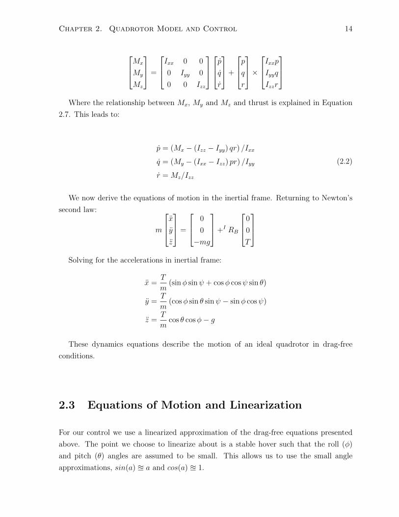
2.3 Equations of Motion and Linearization
For our control we use a linearized approximation of the drag-free equations presented
above. The point we choose to linearize about is a stable hover such that the roll (φ)
and pitch (θ) angles are assumed to be small. This allows us to use the small angle
approximations, sin(a) u a and cos(a) u 1.

Chapter 2. Quadrotor Model and Control 15
Taking the small angle approximation for roll and pitch in Equation 2.2:
x =T
m(φ sinψ + θ cosψ)
y =T
m(θ sinψ − φ cosψ)
z =T
m− g
(2.3)
This can be written in matrix form and the angles for roll and pitch isolated:
[x
y
]=T
m
[cosψ sinψ
sinψ − cosψ
][θ
φ
]⇐⇒
[θ
φ
]=
m
gT
[cosψ sinψ
sinψ − cosψ
][x
y
](2.4)
As is the case in [27], we then assume that the angles in question are small enough
that the body angular rates of the quadrotor are approximately equivalent to the inertial,
or that: φθψ
=
pqr
(2.5)
Combining this with Equation 2.2:
φ =(Mx − (Izz − Iyy) θψ
)/Ixx
θ =(My − (Ixx − Izz) φψ
)/Iyy
ψ = Mz/Izz
(2.6)
The forces acting on the quadrotor are thrusts derived from the rotation of the rotors
and gravity, as can be seen in Figure 2.3. In general, this speed can be approximated as
being proportional to ω2, where ω is the rotation speed of the rotor. The methods used
to control a quadrotor typically involve either setting each motor thrust (T1, T2, T3, T4)
independently or controlling the total Thrust (T = T1 + T2 + T3 + T4) and the Moments
about the axes of the quadrotor (Mx,My,Mz). The most common combination for the
moments is to set the moments such that they control the body angular accelerations p,
q and r. The latter method is chosen in this thesis. It is simply a linear combination of

Chapter 2. Quadrotor Model and Control 16
controlling the first method, with the linear combination given by:u1
u2
u3
u4
=
T
Mx
My
Mz
=
1 1 1 1
0 −d 0 d
−d 0 d 0
−µ µ −µ µ
T1
T2
T3
T4
(2.7)
Where d is the distance from the center of mass to the center of the propeller (see
Figure 2.3), and µ is a constant relating the torque to the rotation speed of the motors
Equation 2.6 gives the means of control of the body rates. That is, we can rear-
range to express the moment as a function of the moments of inertia and the current
angles/angular rates:
Mx = (Izz − Iyy) θψ + Ixxφ
My = θIyy + (Ixx − Izz) φψ
Mz = ψIzz
The equations describing the state of the quadrotor are therefore:
d
dt
x θ
y φ
z ψ
x θ
y φ
z ψ
=
x θ
y φ
z ψ
T
m(θ cosψ + φ sinψ)
(Mx − (Izz − Iyy) θψ
)/Ixx
T
m(θ sinψ − φ cosψ)
(My − (Ixx − Izz) φψ
)/Iyy
Tm
cos θ cosφ− g Mz/Izz
, (2.8)
This shows us what our inputs should be as a function of the other variables in the
system in order to control angular rates:
U1 =T
mcos θ cosφ− g
U2 =(Mx − (Izz − Iyy) θψ
)/Ixx
U3 =(My − (Ixx − Izz) φψ
)/Iyy
U4 = Mz/Izz
(2.9)
Where U1 through U4 represent the inputs to the quadrotor controller.

Chapter 2. Quadrotor Model and Control 17
2.4 Summary
This Chapter introduced the reference frames in use in this thesis, as well as developing
the drag-free equations of motion for the quadrotor.

Chapter 3
Image Based Visual Servoing
Image-Based Visual Servoing (IBVS) is a form of visual servoing where the error to be
minimized is expressed directly in the image frame. This is a well-established algorithm
in the visual servoing field that was traditionally used on fully actuated systems. This is
in large part due to the difficulties associated with implementing IBVS on underactuated
platforms.
In order to successfully implement IBVS on underactuated systems, researchers have
made modifications to the traditional IBVS algorithm. In this chapter, the traditional
IBVS scheme is presented. This development follows those in many IBVS texts ([6] and
[27] for example) with the new contribution of this development being the addition of
a moving target. Then the implementation of the virtual camera is explained. The
modification of IBVS to include a moving desired image is the main contribution of this
chapter, and simulations verifying all of the above are presented. Finally, the advantages
of this moving desired image implementation are explained.
3.1 Classical Image-Based Visual Servoing
The foundation of classical IBVS is the relation between the velocity of the camera and
movement of the a single image point in the image:
s = Levc (3.1)
Where s = [x y]T is a point of interest in the image, Le is the image Interaction Matrix
or Feature Jacobian, and vc is the camera velocity in the inertial frame. The essence of
this relationship is the interaction matrix, which describes how the image feature moves
18
Chapter 3. Image Based Visual Servoing 19
depending on the velocity of the camera.
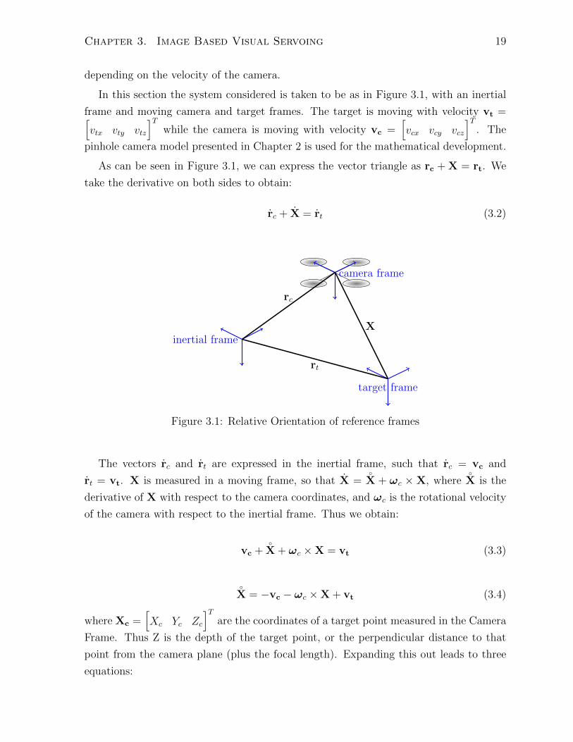
In this section the system considered is taken to be as in Figure 3.1, with an inertial
frame and moving camera and target frames. The target is moving with velocity vt =[vtx vty vtz
]Twhile the camera is moving with velocity vc =
[vcx vcy vcz
]T. The
pinhole camera model presented in Chapter 2 is used for the mathematical development.
As can be seen in Figure 3.1, we can express the vector triangle as rc + X = rt. We
take the derivative on both sides to obtain:
rc + X = rt (3.2)
camera frame
X
target frame
rt
inertial frame
rc
Figure 3.1: Relative Orientation of reference frames
The vectors rc and rt are expressed in the inertial frame, such that rc = vc and
rt = vt. X is measured in a moving frame, so that X =◦X + ωc × X, where
◦X is the
derivative of X with respect to the camera coordinates, and ωc is the rotational velocity
of the camera with respect to the inertial frame. Thus we obtain:
vc +◦X + ωc ×X = vt (3.3)
◦X = −vc − ωc ×X + vt (3.4)
where Xc =[Xc Yc Zc
]Tare the coordinates of a target point measured in the Camera
Frame. Thus Z is the depth of the target point, or the perpendicular distance to that
point from the camera plane (plus the focal length). Expanding this out leads to three
equations:

Chapter 3. Image Based Visual Servoing 20
Xc = −vx + vtx + ωzYc − ωyZcYc = −vy + vty + ωxZc − ωzXc
Zc = −vz + vtz + ωyXc − ωxYc
(3.5)
Take the derivative of the projection equations (2.1):x =
fXc
Zc− fXcZc
Z2c
y =fYcZc− fYcZc
Z2c
(3.6)
Using Eqn. (3.5) in (3.6) the following are obtained:
x = −vcx − vtxZ
+ xvcz − vtz
Z+ xyωcx − (1 + x2)ωcy + yωcz
y = −vcy − vtyZ
+ yvcz − vtz
Z+ (1 + y2)ωcx − xyωcy − yωcz
Which can be split into matrix form:[x
y
]=
[−1/Z 0 x/Z xy −(1 + x2) y
0 −1/Z y/Z 1 + y2 −xy −x
][vc
ωv
](3.7)
which is of the form of equation 3.1. Thus:
Le =
[−1/Z 0 x/Z xy −(1 + x2) y
0 −1/Z y/Z 1 + y2 −xy −x
]
and
vct =
vcx − vtxvcy − vtyvcz − vtzωcx
ωcy
ωcz
(3.8)
leading to the Image Kinematics equation:
s = Levct (3.9)

Chapter 3. Image Based Visual Servoing 21
Remark
The development of IBVS in a static image target case leads to the exact same rela-
tionship as Equation 3.9, just with vc as opposed to vct. In other words the performance
of IBVS when the target’s motion is known will be identical to the case of IBVS with a
static target.
3.1.1 IBVS Control Law Design
The kinematics of the image points with respect to camera and target motion are now
utilized to form a velocity controller for the overall system. The target considered will
be the four corners of a square or rectangle. This has several advantages:
• Rectangles are commonly occurring - they may have an identifying feature to enable
detection of orientation. An example of this would be one corner having a specific
color.
• Many common Computer Vision algorithms detect squares (QR Codes, AprilTags,
rectangle detectors) - these typically include point identification and tracking for
their corners, otherwise one of the challenges of IBVS implementations
• Reduces the number of minima the algorithm may be attracted to. According
to [12], 3 points is insufficient to solve the Perspective and Point (PnP) problem
uniquely. This means that if using only 3 points multiple viewpoints that would be
indistinguishable from either the PBVS or the IBVS implementation. Using four
points avoids this problem.
In implementation there is then a set of image features s =[x1 y1 x2 y2 x3 y3 x4 y4
],
and a desired set of image features which are defined to be s∗ =[x∗1 y∗1 x∗2 y∗2 x∗3 y∗3 x∗4 y∗4
].
The feature Jacobian is then built by stacking four of the previously mentioned Jacobians,
one for each point. This means that Le ∈ R8×6 . The error is defined to be:
e(t) = (s(t)− s∗)
In order to obtain rapid decrease in the error, an exponential decrease in error is
specified. This has the benefit of leading to straight trajectories in the image plane:
e = −λe
Considering the fact that e = s because s∗ = 0, the following is obtained:

Chapter 3. Image Based Visual Servoing 22
e = s = −λe (3.10)
Levct = −λe
vc = −λL+e e (3.11)
Where L+e is the Left Moore-Penrose Pseudo Inverse of Le, necessary because Le ∈
R8×6 and is thus not invertible.
L+e = (Le
TLe)−1Le
T
3.1.2 IBVS Control Law Architecture
Now that the velocity control law has been obtained, it is time to look at the general
implementation of this control law.
Fortunately, as mentioned in Chapter 1 most of the controllers implemented on mul-
tirotor UAVs are nested PID loops. This means it is fairly easy to create a velocity
controller as it actually requires one fewer loop than a position controller. As this is the
more common form of the control architecture and it will be used further along in this
thesis, it is presented below:
Figure 3.2: Quadrotor IBVS control architecture
As can be seen the height and yaw controllers are decoupled and quite a bit simpler
than the horizontal control. This is due to the underactuation of the quadrotor which

Chapter 3. Image Based Visual Servoing 23
brings about the necessity to control the roll and pitch for lateral motion. Thus there
are three nested loops that successively control horizontal velocity and outputs a desired
roll/pitch, which is then fed into a roll/pitch rate controller which outputs our desired
angular accelerations for pitch and roll. These are what the inputs to a quadrotor typ-
ically are. A stability proof for these nested loops is presented in [27] for the linearized
quadrotor model presented in Chapter 2.
3.2 Virtual Camera IBVS
The underactuated properties of the quadrotor mean that although the IBVS algorithm
outputs 6 desired velocities which if followed will push the system towards the desired
equilibrium point, the quadrotor is unable to follow those reference trajectories. Indeed,
it is not possible to independently specify a roll or pitch angle as well as a position.
This implies that a large subset of potential final desired points are not achievable with
a quadrotor UAV - anything involving a static position and a roll or pitch angle, for
example. A quadrotor is unable to maintain a 10 degree pitch while staying above a
stationary target, because for a quadrotor motion in the x-y plane is linked with roll and
pitch. Such complexity is avoided in this thesis where only one position is considered:
being directly overtop of the target.
The problem which motivates the creation of the Virtual Camera is visually explored
in Figure 3.3, where the quadrotor has been tasked with stabilizing above a target. In
order to reach the target, it must tilt towards the target, which increases the error. This
error increase would be perceived by the IBVS algorithm as something that must be
corrected - however our plant is unable to decrease the roll or pitch while correcting for
the horizontal error. As a matter of fact, the outputs of IBVS for roll and pitch are
simply ignored by classical IBVS algorithms on multirotors.
At the same time as an angular velocity command is created by the tilting, another
effect is an increase in the commanded velocity to correct for the perceived increase in
error. Once the quadrotor has accelerated enough to reach the desired velocity, it will be
able to reduce the tilt angle and reduce this effect. This leads to oscillations, as will be
seen in the simulation results.
As was mentioned briefly in Chapter 2, quadrotor actuators allow control over four
degrees of freedom. Two main choices are possible. One is to control the angles (more
accurately, the angular rates) and the total thrust. Another is to control the velocities in
the Cartesian directions, as well as the yaw angle. In the end both methods control the
same four actuators and there is no fundamental difference between the two methods.

Chapter 3. Image Based Visual Servoing 24
Figure 3.3: Virtual Camera motivation
The only difference is in calibration and inner loop expected inputs (i.e. in one case an
inner loop was removed).
It should be recalled here that the mathematical model utilizes drag-free equations
of motion. This means that a constant angle leads to constant acceleration. Thus in
the model a constant velocity quadrotor will be level. In the experimental segment drag
acts on the quadrotor, and a constant angle will lead to acceleration up until lateral drag
equals the lateral acceleration imparted by the current thrust/attitude, at which point the
quadrotor is traveling at a given velocity. As such, a constant angle will equal a constant
velocity after a short period of time in the real-world implementation. This means that
an error will be present in the image even when the desired position is attained directly
overtop of the image. In either case once the horizontal error is zero, the quadrotor will
have passed its target and must now correct back in the other direction. This leads to
oscillations and can lead to instability. This means that a quadrotor tracking a moving
target in real experiments will experience difficulties if some form of compensation for
roll and pitch angles is not introduced.
There are four solutions that are available to reduce the difficulties experienced using
traditional IBVS with an underactuated platform - they were mentioned in Chapter 1.
The two most common ones are the spherical camera approach and the virtual camera
approach. The former uses a spherical camera projection (i.e. treat the camera using a
spherical projection), which then can be de-rotated to always be referenced from vertical
[14].
The latter is used here and involves utilizing the known or approximated roll and pitch
of the quadrotor to correct the image plane to be facing straight down [19], [27]. This
method maintains the standard planar projection or pinhole camera model.
Remark:
The virtual camera frame referenced in section 2.1 has its origin at the same place
as the camera reference frame and is mathematically de-rotated from the roll and pitch

Chapter 3. Image Based Visual Servoing 25
motions of the quadrotor. An easy hardware solution to this problem is available and
involves adding a gimbal. The disadvantage to this is that a gimbal adds complexity,
points of failure, weight and cost. The mathematical virtual camera is nearly as effective
- nearly because although the measurements can be de-rotated, the field of view of a
physical camera is a significant limitation for target tracking tasks. A gimbaled camera
is able to maintain the same field of view footprint around the quadrotor independent of
its tilt and roll (assuming no obstacles to the Field of View like landing gear are present),
whereas a fixed camera may lose a significant portion of its field of view while executing
horizontal maneuvers. Using a gimbal to optimize the scene a camera is looking at is
investigated in other research, such as that done by N. Playle in [25]. In terms of landing
a UAV, this is also incorporated in other research such as that by Wenzel et al. [36].
Unfortunately, the drawback of utilizing the virtual camera approach is that an esti-
mated depth must be calculated for each of the points considered. While generally this
is not as computationally intensive as PBVS, it does take additional computation power.
The development is the following:
1. Given points
[x
y
]in the camera frame
2. Reconstruct the vector P =[Xc Yc Zc
], the coordinates of the point P in the
camera frame.
Xc =(x− x0)Zc
f
Yc =(y − y0)Zc
f
3. Use the coordinates in the camera frame and the roll/pitch angles of the camera
to calculate the cartesian coordinates relative to the virtual frame by applying the
rotation matrix formed by the roll and pitch (and optionally yaw) anglesXcv
Ycv
Zcv
=
cosφ 0 − sinφ
− sinφ sin θ cos θ − sin θ cosφ
cos θ sinφ sin θ cos θ cosφ
Xc
Yc
Zc
4. Calculate the virtual image points
[xv yv
]using the coordinates calculated in the
previous step.

Chapter 3. Image Based Visual Servoing 26
[xv
yv
]=
[Xcvf/Zcv + x0
Ycvf/Zcv + y0
]
The focal length appears in both the first and the final steps of this and effectively
cancels itself out. This means that although we include it in the calculations, the camera
calibration does not actually affect the virtual camera computations. As well, the final
addition of the camera center coordinates often does not take place, because computations
for the IBVS algorithm are done with respect to the center of the V frame.
In this thesis yaw was not taken into account for virtual camera calibrations. There
are four reasons for this:
• The math is simplified
• Display of the final values on the image is more intuitive
• Control of the quadrotor is effected in body-frame - if a correction were introduced
for yaw, it would need to be removed before a command was sent to the UAV
• One fewer sensor value to read/rely upon
3.3 IBVS with Non-Static Desired Image
There are many desirable characteristics of IBVS like its low computational load and its
tendency to keep points in the image. However, there are four main disadvantages as
well:
1. Lack of global stability - can be attracted to local minima
2. No proof of region of stability. This is due to the numerical complexity of the
feature Jacobian.
3. Certain types of image plane errors lead to undesired motions. The classic example
of this is a yawing motion, which leads to a large motion in the z direction.
4. Objects can leave the Field of View of the camera
In an effort to reduce some of these deficiencies, this thesis developed IBVS with non-
static desired image. What is meant by this is that the s∗ = s∗(t), such that s∗ 6= 0. In
other words the desired image points be a function of time. The theory behind this is

Chapter 3. Image Based Visual Servoing 27
that the system will remain closer to the equilibrium point by keeping the desired points
close to the current ones and only moving them to the final desired position during a
period of time. IBVS is known to be stable for a region around the equilibrium point.
Remaining closer to the equilibrium point may also enable higher gains on the non-
static IBVS system. Perhaps more importantly, the initial control inputs experienced
when IBVS is switched on are lower. While this is the same initially as a switching
control where initial and intermediate waypoints are available, this technique is easier to
analyze and could eventually lead to path-planning for the UAV itself. What is meant
by this is that if the control of image points is accurate enough, a trajectory in image
space could be designed that would result in a desired path being flown by the UAV. The
method therefore helps with numbers 2-4 above.
3.3.1 Proof of stability for moving desired image
First a Lemma is presented, which is Theorem 4.18 from Khalil’s Nonlinear Controls
textbook [18]:
Lemma 1. Let D ⊂ Rnbe a domain that contains the origin and V : [0,∞)×D → R is
a continuously differentiable function, such that:
α1(‖x‖) ≤ V (t, x) ≤ α2(‖x‖) (3.12)
∂V
∂t+∂V
∂xf(t, x) ≤ −W3(x),∀‖x‖ ≥ µ > 0 (3.13)
∀t ≥ 0 and ∀x ∈ D, where α1 and α2 are class K functions and W3(x) is a continuous
positive definite function. Take r > 0 such that Br ⊂ D and suppose that
µ < α−12 (α1(r))
Then, there exists a class KL function β and for every initial state x(t0) satisfying
‖x(t0)‖ ≤ α−12 (α1(r)), there is T ≥ 0 (dependent on x(t0) and µ) such that the solu-
tion satisfies:
‖x(t)‖ ≤ β(‖x(t0)‖, t− t0),∀t0 ≤ t ≤ t0 + T (3.14)
‖x(t)‖ ≤ α−11 (α2(µ)),∀t ≥ t0 + T (3.15)

Chapter 3. Image Based Visual Servoing 28
Moreover, if D = Rn and α1 belongs to class K∞, then the previous two equations
hold for any initial state x(t0), with no restriction on how large µ is.
In the above lemma, a class K function is a continuous function α : [0, a) → [0,∞)
which is strictly increasing and has α(0) = 0. It is further K∞ if a =∞ and α(r)→∞as r →∞.
A class KL function is a continuous function β : [0, a) × [0,∞) → [0,∞) if, for each
fixed s, the mapping β(r, s) is class K w.r.t. r and, for each fixed r, the mapping β(r, s)
is decreasing w.r.t. s and β(r, s)→ 0 as s→∞In IBVS, four image points are controlled. The development is identical to the one
presented at the beginning of this Chapter up until Equation 3.10. This relationship no
longer holds because s∗ 6= 0
Maintain the exponential decrease of the error specified originally, where the error is
defined by e = −λe. Taking the time derivative of the error equation now yields:
e(t) = s(t)− s∗ (3.16)
Thus: −λe = Levct − s∗
This is rearranged to obtain a desired control law, with the input being vct:
vct = L+e (−λe + s∗) (3.17)
Here the left Moore-Penrose pseudo-inverse is utilized: L+e = (LT
e Le)−1LT
e
This is the control law. Define a Lyapunov function:
V =1
2‖e‖2 (3.18)
V = eTe
Equation 3.16 applies, which leads to:
V = eT [s(t)− s∗] (3.19)
where again substituting in Equations 3.9 and 3.17:
V = eT [LeL+e (−λe + s∗)− s∗] (3.20)

Chapter 3. Image Based Visual Servoing 29
Expand to obtain:
V = −λeTLeL+e e + eTLeL
+e s∗ − eT s∗ (3.21)
Here define Λ = (1− LeL+e )
V = −λeTLeL+e e− eTΛs∗
It is easy to see that:
eTy ≤ 1
2eTe +
1
2yTy
set y = Λs∗, to obtain:
eTΛs∗ ≤ 1
2eTe +
1
2s∗TΛTΛs∗
Thus:
V ≤ −λeTLeL+e e +
1
2eTe +
1
2s∗TΛTΛs∗
Define: P = (λLeL+e −
12
)
In this case there is a quadratic form of a non-symmetric, square, real matrix. Due to
the quadratic form eTPe , only the symmetric part of P will affect the result:
Ps =P + PT
2
Because this part is symmetric and square, its eigenvalues will be real. We further
assume that Ps is positive definite. This allows the following to be written:
V ≤ −λmin(Ps)‖e‖2 +1
2s∗TΛTΛs∗
Similarly, it is easily proven that ΛTΛ is positive semi-definite.
Then: s∗TΛTΛs∗ ≤ λmax(ΛTΛ)‖s∗‖2
V ≤ −λmin(Ps)‖e‖2 + λmax(ΛTΛ)‖s∗‖2
This is an equation of the form by2 − ax2, so the first thought is to factorize into
(√by +
√ax)(√by −
√ax):(√
b
√‖s∗‖2 +
√a
√‖e‖2
)(√b
√‖s∗‖2 −
√a
√‖e‖2
)
Chapter 3. Image Based Visual Servoing 30
The first term is always positive. For the result to be negative, the second term must
be negative. As a result, the requirement is that:
√b
√‖s∗‖2 −
√a
√‖e‖2 ≤ 0
‖e‖2 ≥ b
a‖s∗‖2
Thus if ever the error is larger than
√λmax(Λ
TΛ)
λmin(Ps)‖s∗‖, the Lyapunov function deriva-
tive will be negative. If this is the case the error will return to below the limit. Note
that this does not guarantee the error’s behaviour when smaller than this limit. As such
it is not possible to ascertain when the error might be zero so long as the desired image
points are moving. The error will converge to zero once the points have stopped moving,
as is proven in [6].
Return to the inital lemma. We seek class K functions - which are defined as being
continuous, [0, a) → [0,∞), strictly increasing, and having α(0) = 0. A function is K∞
if it also has that a =∞ and α(r)→∞ as r →∞.
α1(e) =1
4‖e‖2 and α2(e) = ‖e‖2 are selected
These are continuous, strictly increasing, α1(0) = α2(0) = 0. In addition, they go to
infinity as e goes to infinity. They are thus K∞ functions, and satisfy equation 3.12:
1
4‖e‖2 ≤ 1
2‖e‖2 ≤ ‖e‖2
For future reference, the inverse of these two functions are: α−11 (e) = 2√
e and
α−12 (e) =√
e
W3 needs to be a continuous positive definite function - in this case pick W3(e) =
limc→0+
ce2. This means that for reasonable values of e and s∗, the function W3(e) ≈ 0.
Because V (e) ≤ 0 is true for e ≥
√λmax(Λ
TΛ)
λmin(Ps)‖s∗‖, and W3(e) ≈ 0, in equation
3.13 µ can be set to µ =
√λmax(Λ
TΛ)
λmin(Ps)‖s∗‖ + 0.1. The reason for the 0.1 is because
V must be negative at all times for µ ≥ ‖e‖, and it is possible to have V = 0 when
µ =
√λmax(Λ
TΛ)
λmin(Ps)‖s∗‖.
The section about r in the proof is not required, as there are no restrictions on µ.

Chapter 3. Image Based Visual Servoing 31
Indeed, D = Rn and α1(e) is K∞, so that the equations below hold for all x(t0), with no
restrictions on µ.
Thus we have satisfied the conditions of Theorem 4.18 from Khalil’s book, and there
is a time T such that:
‖e(t)‖ ≤ β(e(t), t), ∀ 0 ≤ t ≤ T (3.22)
‖e(t)‖ ≤ 2µ, ∀ t ≥ T (3.23)
Or, more useful still: ‖e(t)‖ ≤ 2
√λmax(Λ
TΛ)
λmin(Ps)‖s∗‖max + 0.2, ∀ t ≥ T
Where β is an unspecified KL class function. Note that the dependence on t0 was
dropped because our system is autonomous, i.e. the dynamics do not change with time.
This concludes our proof.
We interpret this proof to mean that the observed error will be bounded by the speed
of the motion of the desired image, scaled by the eigenvalues of the matrices Ps and
ΛTΛ.
This assumes that the camera is able to instantly accelerate to the desired value - in
other words it does not take into account the dynamics or controller on the quadrotor.
3.4 Landing strategies and applications to image-
based approaches
There is a large literature on landing strategies for various flying craft. The one to
choose for a given application depends on the priorities - minimum time to landing (a
switching scheme would be best), minimum energy, maximum robustness, simplicity, etc.
Two main approaches that were considered promising in the literature are considered,
and some of the ramifications these approaches have in an image-based visual servoing
framework are explored.
3.4.1 Approaches to landing maneuvers
The two major approaches to a landing in the literature have been constant descent speed
approaches (e.g. [2]) or Tau Theory landings (e.g. [33]), in which a ratio of the descent
speed over the height is maintained; i.e.z
z= C.

Chapter 3. Image Based Visual Servoing 32
The first approach is the simplest to implement, and overall seems to work quite well.
Variations on this theme will have different approach speeds depending on the height -
though in the end, there is one speed for landing. Typically this downwards speed will
be reduced just before contact with the ground by ground effect, and as such landing is
smoother than the specified descent speed.
The latter approach is more elegant, and appears to be used by insects such as bees
to allow them to touch down quite smoothly even on precarious perches. This approach
was investigated experimentally in [33]. This approach has one major disadvantage that
precludes its use in this study - it is unstable when the magnitudes of z or z are small,
which means at the beginning or towards the end of a maneuver. This approach is more
likely to be successful when accurate data is available at high rate to the control system.
3.4.2 Image-Based landings
Intuitively, it is easy to think of what would be seen while landing overtop of a square.
All of the corners of the square should move out towards the edge of the image. Math-
ematically, we recall for the reader’s convenience Equation 2.1: x =fXc
Zc+ x0. In order
to have Zc → 0, which corresponds to a landing, there are two options. Either Xc can go
to infinity, or x can go to infinity. It is clear that for the case of a controlled landing, the
latter is preferable. With a single point, it is not mathematically possible to distinguish
between the two cases.
As a result it is necessary to have two points - separated by some distance L. In this
case a one-dimensional situation is considered, but it is trivial to extrapolate this to a
2D square. In order to effect a landing between P1 = (−l) and P2 = (l), the following is
a necessary condition: −l ≤ XA ≤ l where XA is the position of the aircraft. This means
that in this case Xc1 ≤ 0 and Xc2 ≥ 0.
Thus a landing will be ensured so long as x1 or x2 is zero while the other is ±∞, or
x1 and x2 go to ∞ with opposite signs. In the case considered, with four points in 2D,
again the requirement will be that they all increase in opposite directions, i.e.: the four
points must go to: (∞,∞), (∞,-∞), (-∞,∞), and (-∞,-∞).
On a practical note, having any of these points go to infinity while maintaining them
in the field of view of a camera is an unrealistic expectation. However, in practical
applications three solutions offer themselves to the user. One can lift the camera above
the landing gear of the craft, such that even when the quadrotor is on the ground the
camera maintains a good field of view. Another solution is to have nested landing tags,
which will be cycled through as the craft approaches the ground. In this fashion one can

Chapter 3. Image Based Visual Servoing 33
have extremely small landing tags on landing which will be able to be seen even quite
close to the ground. A third solution which is often employed is to simply shut off the
motors from a height when directly above the target. Although this runs the risk of
damaging the quadrotor, it is an effective way of ensuring that the landing is completed
directly on top of the target. It is also a good way to avoid any potential difficulties
associated with Ground Effect.
The above discussion brings up a further consideration in multirotor landings. It is
often advantageous in image-based approaches to limit the control inputs of a quadrotor
to tighter limits when approaching the ground. This is because closer to the target the
same image error may actually correspond to quite a bit less distance that the plant
needs to correct for. For example [2] use height as a gain scheduling component with
three specific thresholds to ensure that their quadrotor is not too aggressive closer to the
ground. This seems to have been done empirically rather than according to theoretical
control design. In this case the tradeoff is between controllability and maintaining field
of view of the camera.
3.5 Simulations work
In this section the Quadrotor system and a visual target are simulated in Matlab/Simulink.
The system simulated is meant to mimic the physical characteristics of the experimental
platform, the Parrot Ardrone 2.0:
Table 3.1: Ardrone physical properties
mass 0.42kgarm length 0.18mIxx 0.0241 kg ·m2
Iyy 0.0232 kg ·m2
Izz 0.0451 kg ·m2
Note that here the arm length is taken as being from the center of the Ardrone to the
motor mount. It is thus half of the rotor-to-rotor distance.
The drag-free model presented in Chapter 2 is used for the simulations, and the
simulation assumes that the quadrotor is able to produce moments around the three
axes and the total thrust desired. As such, the coefficients of thrust or drag of the
motors are left unspecified. In the simulations, the assumption is that the quadrotor is
able to produce arbitrary values of moments and thrust in an instantaneous fashion.

Chapter 3. Image Based Visual Servoing 34
Note that this simplified model of the quadrotor ignores many elements affecting the
real-world Ardrone. The primary concern is that a Field of View is not implemented on
this simulation. Although it is possible to determine if the target leaves the FOV it is
assumed that even when outside of the FOV the algorithm is able to obtain feedback.
Drag is ignored, despite being a large factor for a UAV such as the Ardrone which has a
foam shell. As mentioned above the assumption of the simulation is that the quadrotor
can attain any thrust or moment desired. This is a reasonable assumption for small
motions about hover - however in a real experimental platform there will be limits to
the amount of thrust or the moments that could be produced, and the speed with which
those could be applied. As such, it is necessary to interpret the simulation results with
the above limitations in mind.
The PID gains used in this are shown in the table below. This simulation with all the
same parameters is used throughout this thesis whenever a simulation is mentioned.
Table 3.2: PID controller gains
P(x)d I(x)d D(x)d P(y)d I(y)d D(y)d Pθd Iθd Dθd Pφd Iφd Dφd
2 0 0 2 0 0 30 0 5 30 0 5P(θ)d
I(θ)d D(θ)dP(φ)d
I(φ)d D(φ)dP(z)d I(z)d D(z)d P(ψ)d
I(ψ)d D(ψ)d
1 0 0 1 0 0 0.5 0 0.05 10 0.1 0.5
The numerical simulations work that was carried out to verify the theoretical work
presented above is presented in this section. To begin with the advantages of the virtual
image based visual servoing are shown through simulations comparing it with the classical
Image-Based Visual Servoing scheme. Then simulations showing the performance of the
virtual IBVS as compared with our Non-static desired image virtual IBVS are presented
to show differences in the performance of the two controls. Finally, as the goal of this
thesis is landing simulations where the quadrotor is landing are presented.
3.5.1 Classical and Virtual IBVS
The advantages of using a virtual camera image are presented in this section.
In the simulation results seen in Figures 3.4 and 3.5, the initial conditions are an offset
from center of -3m in x, -2m in y, -15 degree offset in roll and 15 degrees in pitch. It
can be seen in Figure 3.4 that the Virtual IBVS does not perform that much better in
terms of position than the CIBVS scheme. However, Figure 3.5 shows that Virtual IBVS

Chapter 3. Image Based Visual Servoing 35
performs far better than the Classical IBVS. This is evident in the overshoots and longer
settling time of the angles in both the pitch and roll directions.
(a) X Position (m) (b) Y Position (m)
Figure 3.4: Cartesian position of quadrotor with Classic IBVS and Virtual IBVS.
(a) Roll angle in degrees (b) Pitch angle in degrees
Figure 3.5: Angular motion of quadrotor with Classic IBVS and Virtual IBVS.
Again the reason for this is that there is no coupling between the error and the roll
and pitch values for the VIBVS scheme. In the CIBVS scheme, the control input and the
error are coupled and this leads to far greater oscillations than in the VIBVS scheme.
3.5.2 Virtual and Non-Static Virtual IBVS
In this section the responses of the Virtual IBVS and the Non-Static desired image
virtual IBVS are compared. The classical IBVS formulation has a few disadvantages due

Chapter 3. Image Based Visual Servoing 36
to poor conditioning of the interaction matrix. Among those are poor reactions in the
z axis which is the least sensitive in terms of response. It is also an axis that is highly
affected during yawing motions in order to keep image point trajectories straight.
(a) Cartesian Position (b) Yaw angle in degrees
Figure 3.6: Yawing motion of a quadrotor with VIBVS and a Non-Static desired imageVIBVS.
As a result the two algorithms are compared where they are already above the target,
and are commanded a pure yawing motion of 90 degrees as of t=5 seconds. The first one
is a step command change, which would happen if Virtual IBVS algorithm were to be
suddenly turned on. The second one involves a linear change in yaw which commanded
over a period of 5s.
The results of this with the same gains are shown in Figure 3.6. As expected, the
NS-VIBVS method is somewhat slower than a step change. Nonetheless although the
motion takes about twice the amount of time, the motion exhibits nice smooth properties
(for example a much nicer departure from the equilibrium 10m hover) than the standard
method. In addition, although the NS-VIBVS method takes twice the amount of time
it only climbs by about 1m in Z as opposed to the 5m climbed by the classical control
scheme.
This can have significant advantages in real-world scenarios, where for example there
may be limited operational space for the UAV - this is particularly of concern in indoor
environments. More importantly the target being detected may have a limited detection
range due to resolution limits on the camera.

Chapter 3. Image Based Visual Servoing 37
3.5.3 Landing using non-static target images
In this section a quadrotor is hovering offset from a target by 2m in the y direction and
1m in the x direction. The quadrotor is commanded to land, with the desired z following
an exponential decrease in height trajectory. It is shown that the quadrotor performs the
landing and also that the error observed remains within the theoretical limit established
in section 3.3.1.
(a) Cartesian Position (b) Error and Error Limit
Figure 3.7: Landing of a quadrotor using IBVS with non-static desired image.
The simulations shown are without accounting for the dynamics of the system. That
is, these are simply meant to demonstrate what an IBVS response would look like if
the quadrotor plant were to immediately attain the desired setpoints. This is a way of
ensuring that the response is following the stability proof presented.
As can be seen in Figure 3.7, the quadrotor is able to converge within a few seconds to
the desired horizontal position, and it then slowly descends until it reaches approximately
zero at 60s.
The error observed in the second figure appear to be increasing exponentially towards
the end of the simulation. This is due to the desired point motion commanded by the
landing procedure. In our simulations, the quadrotor is essentially represented by its
center of mass. Additionally, the camera is at the center of mass of the quadrotor. This
situation means that a fully ”landed” quad is one where the camera center is on the
ground, meaning that Zc = 0, which in turn means that the image points lie at infinity
on the image plane. Note that in any real quadrotor implementation the camera is not
likely to actually touch the ground when the quad is landed. Indeed, having the camera
touch the ground would be dangerous for the lens in case pebbles or other obstacles were

Chapter 3. Image Based Visual Servoing 38
on the ground. In an ideal case, our camera would be as high as possible off the ground
to maintain a large field of view during the landing. This will be further examined in the
experimental sections of this work.
Even in the case of a camera placed well above the ground, the speed at which the
desired points are retreating towards infinity increases with time. This leads to an in-
crease in the observed image error towards the end of the visual servoing, which is what
is observed in Figure 3.7b . Notice that the error magnitude, while greater than the
magnitude of s∗, always remains below the theoretical limit calculated in Section 3.3.1.
3.6 Summary
This Chapter investigated the theory and simulations using Image-Based Visual Servoing.
A comparison of classic and virtual-camera image-based visual servoing was presented.
In addition, the performance of the virtual camera was demonstated to be better than
that of the classical image-based visual servoing. A means of smoothly varying desired
features so as to maintain better trajectories using IBVS was then presented, along with
a Lyapunov stability proof. These simulations showed better 3D motion characteristics
than equivalent classical IBVS which typically uses step inputs to create motion. Finally,
the application of these moving desired images to the case at hand - landing a UAV -
was presented.
Chapter 4
Position Based Visual Servoing
Position-Based Visual Servoing is the use of image features to calculate a relative 3D
position which is then used to create a control law to regulate the aforementioned position.
As such, it differs from IBVS in that it explicitly uses 3D reconstruction of features prior
to the application of a control law. It is more varied in terms of the controllers applied, due
to the ease of implementing various control architectures once a difference in position is
known. Because the error is a difference in position, it typically uses a position controller
instead of a velocity one.
This theoretical investigation into PBVS mainly furthers a previous investigation in
the Flight Systems and Controls lab [27]. In it a stability proof was presented for static
targets. Here that proof is extended to targets with constant yaw rate.
4.1 Architecture of standard PBVS controls
The control architecture for the PBVS system is similar to that of the IBVS control
system from the previous Chapter in that it involves nested PID control loops to control
the UAV. The major difference in most cases is that there is a PID node on to transform
the position error into a desired velocity. In the case of the simulations presented in
this work, the same gains as shown in the previous chapter for the control system are
maintained. The extra PID is not implemented but left as a simple proportional controller
with a gain of 1 - as if it were not there.
This section furthers the work in [27]. These results presented a nested PID controller
capable of stabilizing the quadrotor overtop of a target. The controller implemented in
the paper was augmented by taking into account the target velocity and acceleration.
The simplest velocity controller for maintaining position above a static target would
39

Chapter 4. Position Based Visual Servoing 40
Figure 4.1: PBVS Architecture
have an error term given by:
xd = xT − xA (4.1)
Where the subscript stands for aircraft. This will be labeled the Position control law
(Position [1]) in the Figures that follow.
Augmenting this into a tracking law for a moving target with feedforward from the
target velocity leads to:
xd = xT +KP (xA − xT ) (4.2)
A saturation function is added to the (xA − xT ) portion in order to ensure that the
motions in the horizontal plane are not overly aggressive. This prevents the quadrotor
from performing aggressive maneuvers and increases the probability of the target staying
within the field of view, which leads to the following desired velocity:
xd = KP xT + λh(xT − xA) (4.3)
Where h(x) =x
1 + |x|is a saturation function. This control law will be labeled
Velocity [2] in the Figures that follow. This is the controller that was used in [27].
It is plausible to consider adding the saturation function to the entire desired velocity
- thus preventing the quadrotor behaving too aggressively even if changes in the velocity
of the target are large. This is addressed later in this Chapter.
Although this control law performs well for the most part, it is still not able to ad-
equately track an accelerating target, which can be seen in Figure 4.2c. Indeed, the
controller lags behind the target temporally and overshoots it spatially. This inspires the

Chapter 4. Position Based Visual Servoing 41
next iteration which is to add a compensation term for the acceleration:
xd = KP2xT +KP1xT + λh(xT − xA) (4.4)
We utilize simulations with various targets to investigate the effects of our controllers
from a theoretical point of view. Three different test cases are used, and all three con-
trollers are used in each case
• Static target, Initial Conditions offset 8m horizontally in x direction
• Constant Velocity target from time t=0, when it is directly below the stationary
UAV
• Circular motion target, 4m radius centered about origin
Results are presented for the x direction, which are representative of those in the y
direction. The controllers lead to the simulation results in Figure 4.2.
(a) Static target (b) Constant Velocity (c) Circular Motion
Figure 4.2: Tracking performance of all three controllers for stationary, constant velocityand circular motion targets (single axis).
(a) Pitch angle, Static Target (b) Constant Velocity Error (c) Circular Motion Error
Figure 4.3: Pitch angle or Error measured for the simulations in 4.2.
It can be seen that using the pure position difference controller the performance of
the controllers is identical. Because the velocity and acceleration reported by the target

Chapter 4. Position Based Visual Servoing 42
are zero and the gains were not modified when adding terms, the controllers behave
identically. Notice that in the case of Figure 4.3, we do not plot the error versus time -
this is because there is no difference between the error e =√
((∆x)2 + (∆y)2) and the x
position, since y=0 in this simulation. More interesting is to see the pitch angle during
this time reaches 20 degrees. The linearized model in this thesis is only accurate near
hover, which is why a saturation term becomes necessary.
Figure 4.2b shows that when the target is moving with constant velocity, the controller
which does not take into account the velocity or acceleration of the target is unable to
adequately track the target. This can be improved by adding integral control, however
this offers very slow convergence and degrades performance on the other axes.
Figure 4.2c shows that the only controller capable of reducing the error to zero overtop
of a constantly accelerating target is that which takes into account both the velocity and
acceleration of the target.
Note that these simulations incorporate no noise or time delays. Results are similar
for moderate time delays (≤0.5s) - this will be examined below. It can be seen that
in all cases adding the acceleration compensation leads to better tracking performance
overhead the target within one cycle.
It is observed that the addition of target information enables the quadrotor to track
the target more effectively. This is expected and common-sense, but it is nonetheless
a good idea to verify it and get an idea of the extent of the performance difference in
simulation before attempting a real-world implementation. In the case of the simple
position controller with a circular motion target, the error can be as significant as 4m.
4.1.1 Simulations with time delays
In the theoretical proofs of stability in [27], time delays were not taken into account.
There is one theoretical work where time delays are taken into account that the authors
are aware of - by Daly and Waslander [8]. The essence of their method is to create a
joint decentralized control of the two vehicles. Each vehicle delays its own measurements
by the time delay to the other vehicle. In this fashion by using Retarded Functional
Differential Equations it is possible to prove the stability of the closed-loop system.
Nonetheless to investigate the effects of time delays on the simulations above, the
same conditions are repeated with a time delay of 400ms between the ground rover and
the UAV. The results are presented in Figure 4.4.
The conditions on this particular set of simulations was to assume a constant delay
meant to represent a communication between the rover and the UAV of 0.4s. Position

Chapter 4. Position Based Visual Servoing 43
difference estimation was assumed to be instant, while the velocity and the acceleration
data are delayed.
(a) X position, 400msec delay (b) Error, 400msec delay
Figure 4.4: Tracking performance and error for all three controllers - target performingcircular motion, with information delayed by 0.4 seconds.
As can be seen in Figure 4.4, with a time delay included there is still a slight advantage
to the acceleration controller - however this advantage is reduced.
4.2 Stability proof for constant yawing rate target
The quadrotor model presented in Chapter 2 shows that the rotation about the z axis is
decoupled from the other controls. As a result, the control design for the desired yaw ψd
is fairly straighforward:
ψd = λψ(ψT − ψA) (4.5)
This design was proven to be stable for targets that had a constant yaw angle - i.e.
that were not rotating about their z axis. Here the proof is extended to targets which are
yawing at a constant rate. This situation may for example be encountered in a ship-based
landing if the ship is turning. To prove this design, an augmented controller is applied:
ψd = λψ(ψT − ψA) + AψT (4.6)
Where A is a constant which will be determined later.

Chapter 4. Position Based Visual Servoing 44
The input to the quadrotor is assumed to be u′4 = ψA (Where A signifies aircraft), and
is given by:
u′4 = Pψ(ψd − ψA) +Dψd
dt(ψd − ψA) (4.7)
Where a PD control for the yaw controller is assumed. This can be expanded to:
u′4 = Pψ
[λψ(ψT − ψA)− ψA + AψT
]+Dψ
[λψ(ψT − ψA) + AψT − ψA
](4.8)
Here the target is assumed to be yawing at a constant rate, so that ψT = 0 Again,
using that ψA = u′4:
u′4 =Pψ
1 +Dψ
[λψ(ψT − ψA) + AψT − ψA
]+
Dψλψ1 +Dψ
(ψT − ψA) (4.9)
Set A=1, define ∆ψ = ψA − ψT and can rearrange into matrix form to obtain:
[˙∆ψ
∆ψ
]=
0 1
− Pψλψ1 +Dψ
− Dψλψ1 +Dψ
− Pψ1 +Dψ
[∆ψ
˙∆ψ
](4.10)
This is the same form of the equation as was given for a static target in Appendix A.1
of [27], thus the proof is the same and is not reproduced here.
4.3 Simulations Work
4.3.1 Yaw simulations
In order to verify the stability of the above control laws, simulations were run for constant
yaw rate target as well as accelerating yaw rate targets. The control laws implemented
were Equations 4.5 and 4.6.
In the first simulated case, the yaw initially starts at 0 before increasing linearly to
180◦, dropping instantly to 0◦ and increasing again to 180◦. It can be seen that the
second control law is able to track the target yaw with zero error, while the first law
maintains a steady state error.
4.4 Saturated total velocity controller
Briefly mentioned above was that the original controllers used, while able to follow moving
targets, had a weakness that was shown in 4.3a. Indeed, it is important to saturate the

Chapter 4. Position Based Visual Servoing 45
(a) Yaw for both models (b) Yaw Error
Figure 4.5: Yaw tracking performance for the Control Laws in Equations 4.5
controllers for large differences in position - this prevents the controller from straying too
far from the model that it was designed to control - that of a quadrotor around hover.
If assumption of near-hover conditions is invalid, the stability of our system can not be
guaranteed.
Also mentioned was one of the drawbacks of the simulations is that they have a lack
of physical boundaries. These boundaries were difficult to establish in the simulations
without data on the total thrust and moments that could be generated by the quadrotor.
This can be seen in the reaction to motion in Figure 4.6, where the quadrotor initially
rolls to over 60 degrees. This is not possible with the physical Ardrone and shows a lack
of fidelity to the quadrotor’s capabilities. Note that the conditions simulated here were
aggressive, in order to highlight potential flaws in the approach.
The solution to both of these problems is to saturate the total output of the control
that gets fed into the velocity controller of the quadrotor. Note that in this investigation
Control Law 1 from the previous section is dropped, as it has shown less promising
performance and is already saturated. Instead in this case a saturated version of the
third control law is explored:
xd = h [KP2xT +KP1xT + λ(xT − xA)] (4.11)
Note that an angle limiting saturation term is often implemented on quadrotor plat-
forms. In addition, the performance of the controller with acceleration, velocity and
position differences in the saturation term will lead to better performance for a subset
of cases where the target is accelerating or moving rapidly towards the quadrotor and

Chapter 4. Position Based Visual Servoing 46
(a) X position, input saturation controller (b) Error, input saturation controller
Figure 4.6: Tracking performance for input saturated versus non saturated controllers.
Figure 4.7: Angle for input saturated versus non saturated controllers
enters the field of view. A representative view of this is provided in Figures 4.6 and 4.7,
where the high velocity and acceleration of the target during the initial second of the
simulation overcomes the position difference error and causes the initial response to be
in the incorrect direction for the non-saturated controller.
Note that this is not an unusual condition, particularly if the velocity of the target
is being measured from backwards Euler difference of the position of the target in the
image. It is often the case that a target will enter a field of view at relatively high velocity.

Chapter 4. Position Based Visual Servoing 47
4.5 Simplified PBVS - S-PBVS
Traditional visual servoing methods were designed for actuators having 6 or more DOF.
Thus they were designed to have feedback to control all of the possible DOF. Although in
some cases it may be helpful to have these extra channels to be controlled, as mentioned
before the quadrotor is only actually able to be controlled in 4DOF. As a result, it is not
necessary in the case of the multirotor to calculate relative orientations other than the
relative yaw - the others are ignored by the control law.
It is desirable to keep everything simple - which usually leads to the most efficient and
foolproof systems. In the case of a quadrotor then, there need not be a full reconstruction
of pose. Particularly in the case of an attempted landing overtop of a level landing pad,
it is only truly necessary to control the three translational degrees of freedom. Indeed,
yaw is only required if the objective is to land with a given orientation with respect to
the target. If the goal is simply to land overtop of a target, yaw can be stabilized to a
given value (call it North) and left there - the feedback obtained by the camera system
is in the Image (and easily transformed to the camera and/or Body) frames, and can be
used without need for yaw corrections of any kind.
To land a quadrotor on a level platform then only requires three degrees of freedom.
A single point on an image has two degrees of freedom. This then leaves one free degree
of freedom. In the case of a quadrotor a simple solution presents itself. A visual control
system for the horizontal degrees of freedom could be implemented using the central point
of a distinct pattern, and the altitude left to be controlled by the size of the pattern.
This pattern could be one of many different things. It could for example be a standard
computer vision tag (ARTag, AprilTag, QR Code, Barcode, etc), it could be a traditional
Helicopter landing pad. In the case of this work, it can be any one of those things. The
area occupied by the feature will be the basis for a height approximation. Note that it is
also possible to get height estimates from other sensors - barometric pressure altimeters
or range finders for example.
Unfortunately, while the rotational degrees of freedom are not directly controlled,
they nonetheless impact the image. To prevent this from occurring the virtual camera
implementation from the previous chapter is utilized for the one single point. This
approach does end up calculating a position difference and implementing a control law
based on that position difference, hence this approach has been classified under the
Position-Based Visual Servoing section. It is noted that if a means of keeping the camera
facing nadir were implemented (i.e. gimbal), this approach would be reduced to an Image-
Based Visual Servoing system. This is a perfect illustration of the difficult decisions
Chapter 4. Position Based Visual Servoing 48
sometimes involved in placing a method squarely within IBVS or PBVS classification.
The development of the correction for roll and pitch is identical to that in the previous
Chapter, so it is not reproduced here.
Note that S-PBVS assumes that the target is perfectly level. This is what enables
the calculation of ∆x and ∆y relative to the roll and pitch. Although in simulation this
is identical to the PBVS methods in previous sections, a difference is observed when
transitioning to the actual aircraft system.
This is in large part due to the ease of processing. In the case of a simple colored blob
above, a few lines in OpenCV or any other image processing software is enough. A blob
has the disadvantage that if only part of it is in the Field of View, the UAV will try to
descend in order to make the blob smaller which is counterproductive.
It is to be noted that one reason for developing this is that the ArDrone and several
other drones come pre-configured to detect the centroid of features, as well as their area.
This makes it easy to implement the above algorithm on various UAV platforms.
4.6 Summary
The motion compensation term seems to be the most important one to add to our control
law. In a real-world implementation, it is also the easiest one to obtain. Theoretically
it may even be obtained by successive differentiation of the error in the image as was
the case in [27], if measurements of the quadrotor position and of the relative position
difference are accurate enough.
Simulations were presented where time delays were taken into account, as well as
comparing and contrasting the saturated input for the velocity control.

Chapter 5
Experimental Setup
This thesis is primarily concerned with the experimental implementation of IBVS and
PBVS on real UAV platforms. This implementation takes place on one quadcopter
platform, the Ardrone2.0. The ground rover utilized is the Create Roomba, because it is
a simple and user-friendly indoor platform
5.1 Optitrack
The Optitrack setup in the lab consists of 6 Flex3 cameras manufactured by Optitrack.
These are connected to a computer running Tracking Tools, the custom Optitrack soft-
ware that runs the reconstruction of position and orientation of user-defined trackables.
The pose of these trackables is measured to sub-millimeter accuracy at 100Hz.
Robot Operating System (ROS) functions purely on Unix-type machines, as such a
second computer running Linux was required. A second desktop computer with Ubuntu
16.04 (Long-Term Support) was chosen. ROS Kinetic was installed. A package imple-
menting a Virtual Reality Peripheral Network (VRPN) client is available for ROS, and
Tracking Tools is able to broadcast VRPN via a user-specified port on IP. Thus by linking
the two computers with an ethernet cable and creating a fixed IP network between the
two, it was possible to receive the Optitrack pose data in ROS.
Tracking Tools software operates in a Left-Handed coordinate system, with the X
and Z axes defining the ground plane, while the Y axis points vertically up. Thus the
following transformations needed to be applied:
XROS = Xopti
YROS = −Zopti
49

Chapter 5. Experimental Setup 50
Figure 5.1: Roomba ground rover with target taped on top
ZROS = Yopti
The same transformations were required for the quaternion values:
qXROS= qXopti
qYROS= −qZopti
qZROS= qYopti
Note that these quaternion values can be different depending on the receiving system.
The above represents the quaternion transformation required for PX4 and ROS.
5.2 Ground rover - the Create Roomba
The ground rover utilized for this experiment is the Create Roomba, a non-holonomic
differential drive two-wheel (plus castering wheel for balance) robot. This is a modified
version of the cleaning robot of the same name, which can accept commanded velocities
input by the user. The create Roomba is controlled from a computer via a USB connection
- it is possible to utilize a radio module to enable distance communications (or Bluetooth
with adequate modifications), but that was not found to be necessary for this project.
The Roomba resembles the more popular Turtlebot, except without a distance sen-
sor (laser or RGB-D sensor). It relies on wheel odometry in order to estimate veloc-
ity/position, and a bump sensor to detect collisions. As a result of imperfections and
uncertainty on measurements, the Roomba will always be turning slightly. There are
two major drawbacks to using the Roomba on this particular project. The first is that
the Roomba offers no feedback as to its status or position. As a result the assumption
has been made that the Roomba has instantly attained whatever desired setpoint has

Chapter 5. Experimental Setup 51
been sent to it. If it has hit an obstacle or is stuck because of a slippery surface, the
program has no way of knowing. The second drawback is that the Roomba has encoders
on its wheels which it spins at a certain rate to detect and control speed. This means
that it is always drifting somewhat in the real-world, because it relies on dead-reckoning
navigation. It is well known that dead-reckoning navigation leads to increasing error over
time.
Both of these issues can be addressed by using the OptiTrack to develop a Roomba
controller. In this thesis such a controller was not developed, because the period of time
during which experiments were run was short enough to not cause problems relying on
the dead reckoning of the Roomba.
5.3 Flying Platform 1: Ardrone 2.0 quadcopter
Figure 5.2: Ardrone 2.0
The ArDrone 2.0 is a very low-cost commercially available quadcopter, manufactured
by Parrot. It consists of a rigid cross frame with foam surrounding the electronics in the
central portion, and along a line to the forward-facing camera. An outer shell of foam
can be added which consists of propeller guards, making the ArDrone safe to fly indoors
- see Figure 5.2. Its physical properties were listed in Table 3.1, so they are not repeated
here.
The Ardrone serves as a good experimental platform for robotics research for three
reasons. To begin with, its low cost makes it easily accessible. It is designed to be
controlled from a phone via wifi, with an SDK that has been leveraged to enable easy
control through computer programming. Ardrone-Autonomy is a package developed at
Simon Fraser University to enable two-way communication with the quadrotor and Robot

Chapter 5. Experimental Setup 52
Operating System (ROS). This means that the ArDrone can easily be fit into existing
or standardized workflows. Images can be processed using the machine vision library
OpenCV which interfaces easily with ROS, saving the user the need to worry about
video pipelines, etc.
The third advantage is that it has two separate cameras as well as downward-facing
sonar for altitude control. The sonar makes altitude control during indoor flying quite
easy, an important advantage. Combined with optical flow which runs on the bottom-
facing camera, the Ardrone can be flown indoors with ease.
The ArDrone suffers from three major disadvantages as well. The first is that video
can only be streamed from one camera at a time. The second disadvantage is that it runs
closed-source firmware on the ARM Cortex A8, which means that users do not get to
access or modify the low-level control algorithms. That can be a significant disadvantage.
An example of this is the aforementioned optical-flow algorithm, which combined with
the sonar sensor allows it to estimate speed. An experiment was run where a mobile
rover with a target on top of it was driving below the ArDrone, which had its propellers
removed so it could not move. The results are plotted in Figure 5.3. It is believed the
optical flow was used in the control of the quadrotor, however due to a lack of source code
it wasn’t possible to fully verify this. The input command to the ardrone appears to be
an angle - not a velocity. Indeed, one observer of the experiment suggested a potential
explanation: that the optical flow was only active during hover. In flight, the command
sent to the ArDrone is an attitude command.
Figure 5.3: Ardrone velocity readings when held immobile
To verify if this was the case a second experiment was set up, where the ArDrone
would hover in one position under OptiTrack control, then manually be given a simple
flight command in one direction (in this case the y direction). The experimenter would
then move a panel with targets on it perpendicular to the flight direction of the Ardrone.
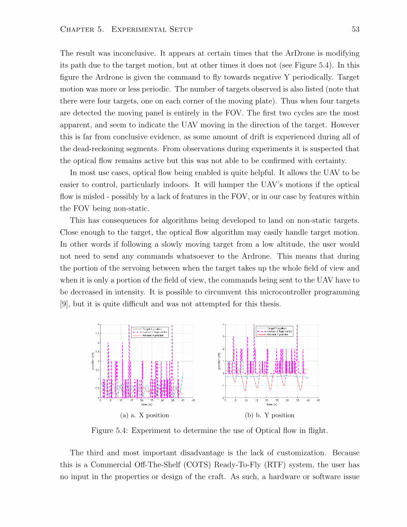
Chapter 5. Experimental Setup 53
The result was inconclusive. It appears at certain times that the ArDrone is modifying
its path due to the target motion, but at other times it does not (see Figure 5.4). In this
figure the Ardrone is given the command to fly towards negative Y periodically. Target
motion was more or less periodic. The number of targets observed is also listed (note that
there were four targets, one on each corner of the moving plate). Thus when four targets
are detected the moving panel is entirely in the FOV. The first two cycles are the most
apparent, and seem to indicate the UAV moving in the direction of the target. However
this is far from conclusive evidence, as some amount of drift is experienced during all of
the dead-reckoning segments. From observations during experiments it is suspected that
the optical flow remains active but this was not able to be confirmed with certainty.
In most use cases, optical flow being enabled is quite helpful. It allows the UAV to be
easier to control, particularly indoors. It will hamper the UAV’s motions if the optical
flow is misled - possibly by a lack of features in the FOV, or in our case by features within
the FOV being non-static.
This has consequences for algorithms being developed to land on non-static targets.
Close enough to the target, the optical flow algorithm may easily handle target motion.
In other words if following a slowly moving target from a low altitude, the user would
not need to send any commands whatsoever to the Ardrone. This means that during
the portion of the servoing between when the target takes up the whole field of view and
when it is only a portion of the field of view, the commands being sent to the UAV have to
be decreased in intensity. It is possible to circumvent this microcontroller programming
[9], but it is quite difficult and was not attempted for this thesis.
(a) a. X position (b) b. Y position
Figure 5.4: Experiment to determine the use of Optical flow in flight.
The third and most important disadvantage is the lack of customization. Because
this is a Commercial Off-The-Shelf (COTS) Ready-To-Fly (RTF) system, the user has
no input in the properties or design of the craft. As such, a hardware or software issue

Chapter 5. Experimental Setup 54
(a) Detection outside of Field of View (b) Detection offset from tag
Figure 5.5: Examples of performance of onboard tag detection
can prevent a project from working. On the software side this can lead to problems such
as the optical flow one above. The most important difficulty in using this device turns
out to be hardware-related - the field-of-view of the bottom-facing camera, which was
only 64 degrees with a 320x240 resolution. In fact, the aspect ratio of the camera is quite
wide. Empirical measurements of the camera found the field of view to be 28 degrees in
the longitudinal direction and 48 degrees in the lateral direction. This created difficulties
during experiments.
5.3.1 PBVS design for Ardrone
The ArDrone contains onboard tag detection for both the forward-facing and downwards-
facing cameras using pre-defined tags. For the downward-facing case, this tag detection
system recognizes oriented roundels. The detection runs at 30Hz and returns the number
of tags detected, the pixel coordinates of the tag center(s) (x, y) and the distance to the
target. This is sufficient information to implement the Simplified PBVS from the previous
chapter.
The main advantage of the onboard tag detection is that there is no need to wait for
the image to be transfered to the ROS ground station and then processed. Indeed, the
required tag information is embedded in the navigation data returned by the ArDrone.
Video framerates from the ArDrone can be variable depending on WiFi signal strength.
They can be as high as nearly 15Hz, or as low as approximately 1Hz, while usually
being in the 7-10Hz range. Although a few obvious factors account for the difference
(obstacles in the way, distance, etc), occasionally the Wifi network was below 1Hz for
video transmission and no reason was found. The onboard tag detection is performed at
30Hz by the bottom-facing camera, more than double the rate that could be hoped for

Chapter 5. Experimental Setup 55
via WiFi. In addition, the reduced processing required on the ground station means that
the time between receiving the tag information and a command being sent is reduced.
The deficiencies of the onboard tag detection are twofold: poor tolerance for illumi-
nation change, and uncertainty in the methods used. Its advantages include the fact
that the tag detection is less dependent on wifi strength, occurs at a faster rate, and is
capable of detecting targets outside of the FOV of the camera. The latter is believed to
be due to the larger sensor size than is actually displayed. The video which is sent to the
computer is either cropped, or the image that the onboard detection runs on includes
pixels outside of the field of view. An example of one advantage and one disadvantage
of the tag detection are shown in Figure 5.5. The onboard tag detection proved easiest
and most robust for this PBVS task.
As was mentioned above, this quadcopter is controlled using Wifi and ROS. The initial
architecture is presented in Figure 5.6.
Figure 5.6: Ardrone control architecture
Initially and for many months experiments were entirely independent of the Optitrack
indoor positioning system. An indoor positioning system was only used for recording
the results of the experiment. As can be seen in Figure 5.6, there was a combination
node called “twist mux”, which is responsible for passing one of the three inputs - either
the keyboard input, the visual servoing algorithm output, or a “zero” twist which just

Chapter 5. Experimental Setup 56
Figure 5.7: Improved ArDrone architecture
tells the ArDrone to hover. This configuration was used because it utilized a lot of pre-
existing code. Indeed, all of the orange nodes in Figure 5.6 were ROS packages that
were available on the repository - in other words one line of code to install and then
customizing of parameters. The only nodes that needed to be written were publishers or
receivers.
Although experiments were successfully run on this architecture, it was difficult to
obtain scientific experiments with it. The main problem was the lack of repeatability -
because the ArDrone was always in a different configuration (speed/orientation) when
it first viewed the target, it was difficult to repeat the experiments. A set of gains that
stabilized the ArDrone successfully in one experiment often failed in the very next try.
Part of this is due to the disturbances acting on the system and inaccurate measurements,
but a large part was this unpredictability.
This led to development of a better control architecture. In this case the OptiTrack
Motion Capture System is used to stabilize the ArDrone slightly offset from the target.
The gains on all of the PID loops of the ArDrone control system are able to be manually
adjusted using the dynamic-reconfigure node in ROS. Outputs from the experiment can
be plotted in-real-time by the rqt plot node of ROS. This makes tuning the system much
easier than the previous system. The new architecture is shown in Figure 5.7.
The new architecture requires fewer, more highly modified nodes as well as a custom-
written PID implementation class. This prevents the need to split the messages into

Chapter 5. Experimental Setup 57
multiple smaller messages each requiring their own nodes. The biggest advantage of this
architecture is that the system will be initialized with approximately zero velocity and
near-hover. The second advantage is that it is possible to run many more experiments
in one given battery than was possible when the system had to be manually flown to an
approximate initial position.
Another advantage is that even if the target is not visible in the Field of View of the
camera, it is possible to have the system maintain its position and climb. The typical
algorithm that was implemented in our case was as follows:
1. If target in FOV:
• calculate relative position
• Add relative position to current position, to find global position of target
• If landing desired, initiate or continue descen
2. If target not in FOV:
• Go to last known target position
• Climb for a user-defined number of seconds.
5.3.2 IBVS design
In addition to the PBVS design shown above, an IBVS Architecture was developed
for the Ardrone. One of the main challenges of a traditional IBVS approach is the
tracking of the image points. That is although identifying a number of points in an
image is straightforward, tracking their progress to the next frame can be challenging.
One approach is to use individual identifiable tags (e.g.: QR codes, bar codes, etc).
Another approach is to use various colors for the four corners. These proved challenging
due to the limited resolution of the ArDrone camera and difficulty in robustly setting
color thresholds.
A second design attempting to solve this problem took a simplistic approach - use a red
rectangle as the target. Select the red elements of the image, erode and dilate to get rid
of remnants, choose the four best corners. This identified the correct corners over 90% of
the time. It was then a question of tracking the four corners. One challenge in this is that
as the drone moves the corners can move significantly in the image. Thus the algorithm
developed calculated distance offsets from the mean point of the four. These distance
offsets were then put into a matrix form, and the measurements were summed up. This
is illustrated in Figure 5.8, where a single column is filled with approximate data in the

Chapter 5. Experimental Setup 58
case where all of the points are in a known orientation. In the case of this algorithm,
the points could be in any given order and thus it was necessary to consider all (4! =)
24 possibilities. This algorithm could perform its task adequately when the features
were correctly tracked, but had poor performance when a point was mislabelled (often
to a jagged edge in the rectangle’s identified area). Unfortunately, the false detections
precluded the use of this algorithm.
Figure 5.8: Yaw rectification algorithm number 1
Because of the difficulties encountered with the above tracking algorithm, a ready-
made algorithm was sought. It was found that corners in the images were most reliably
detected using the built-in OpenCV function ChessboardCorners.
Originally designed and still utilized for calibrating cameras, the Chessboard Corners
algorithm accepts an input image and a size tuple describing the number of rows and
columns in the chessboard. The return value is the (subpixel accurate if desired) pixel
values for each interior corner in the chessboard. It is capable of being run in real time
on an average desktop computer.
This was leveraged to find the four exterior corners of the chessboard. To prevent
excessive yawing motions during initial movement, it was decided that when a chessboard
is newly detected (ie was not detected in the previous video frame), a check would be run
to align the corners detected with the closest possible arrangement of desired corners.

Chapter 5. Experimental Setup 59
This means that the maximum yaw error when a chessboard is first seen would be 45
degrees. Again, this is necessary due to the poor characteristics of IBVS around yawing
motions.
Two algorithms were considered here. The first was already described for the point
tracking above, although because the points were already in order only four sums were
required. This worked, but was overly complex.
A second algorithm and the one that was selected eventually utilized two known points
to rearrange the desired points. Because the ChessboardCorners algorithm returns an
ordered list there are only four possible arrangements of the current detected corners. The
simplest algorithm found was to calculate the angle from horizontal for the 0-1 points.
Using this angle the “desired” points are rearranged such that the 0-1 points follow the
nearest horizontal or vertical from the currently detected points. This is simpler both to
code and to understand than the original algorithm.
The IBVS architecture used is visible in Figure 5.9.
Figure 5.9: Ardrone IBVS Architecture

Chapter 5. Experimental Setup 60
5.4 Summary
This section introduced the experimental platform and laboratory setup that were used
throughout the experiments conducted in this thesis. Advantages and disadvantages of
the setup used were examined - primarily related to ease of use of the Ardrone but its
lack of customizability.
Chapter 6
Experimental Results
Both IBVS and PBVS algorithms were attempted on the first of the two systems from
the previous chapter, and the results are presented below. The second system was ground
tested but not successfully flown using these algorithms.
For PBVS, an 8cm wide visual marker is attached to the top of the Roomba, which is
commanded via ROS to execute a sinusoidal, one-dimensional movement. Imperfection
of the wheels and encoder errors of the Roomba cause the motion to not be perfectly
straight. Due to the single channel of acceleration being applied, the controller which
takes into account the velocity of the target is applied only to the y-axis of the ArDrone.
This is because as is shown in Figure 4.2 there should be no difference given that there
are no reported velocities or accelerations in the x-channel for the Roomba. The x axis
of the quadrotor thus implements PD control purely on position.
IBVS was not tested with the moving Roomba. Instead it used a 6x5 chessboard
pattern printed as large as possible on an 8.5”x11” sheet of paper.
Note that in this chapter the Z direction positive is referred to as up. This is simply
for ease of reading.
6.1 Optitrack setup
Tuning for the Ardrone/Optitrack system was quite straightforward. The controller
under OptiTrack treats the ArDrone as a double-integrator system and is tuned using
the standard ζ and ωn parametrization of rise time and settling time (with ζ = 0.85 and
ω = 1.1). Although that is what was implemented in code, this is equivalent to a PD
control with gains Kd = 1.87, Kp = 1.21. These gains were found to not be responsive
enough, as can be seen in Figure 6.1a, where the Ardrone is commanded to hover at a
position of (X=0, Y=0, Z=0.5). This is likely due to the angle limit that was imposed
61

Chapter 6. Experimental Results 62
on the quadrotor outputs. As a result the gains were multiplied fourfold (to Kd = 7.48,
Kp = 4.84), which led to Figure 6.1b. This shows gains slightly higher than those used
during future experiments (Kd = 5.61, Kp = 3.63). The gains are quite aggressive but
they are able to accurately maintain the position of the Ardrone to within approximately
5cm horizontally, leaving only a 10cm diameter region in which the ArDrone will usually
be found. This allows us to position the visual target within the FOV of the ArDrone.
In the end, a slightly less aggressive control was chosen during experimentation in order
to decrease the oscillations in position.
(a) a. Bad gains Kd = 1.87, Kp = 1.21(b) b. Increased gains - Kd = 7.48, Kp =4.84
Figure 6.1: Ardrone tracking a setpoint of (x=0,y=0,z=0.5) for different gains underOptiTrack control.
6.2 ArDrone 2.0 PBVS Results:
6.2.1 PBVS without Optitrack information
Here the results are presented from the system without using the OptiTrack positioning.
Although the system is capable of hovering over the top of the target for sometimes
extended periods, it is only capable of doing so at altitude. Indeed, hover experiments
carried out below 1-1.5m were generally unsuccessful. It was possible to hover for over
2 minutes with an altitude above 2m - outside of the Optitrack area. The lower the
Ardrone was the smaller the footprint of the camera was on the ground, and the more
often the target would exit the FOV. This led the system to sometimes fail. A method
of “dead reckoning” in the case of the target exiting the field of view was developed but
not tested. This involved flying in the direction the target was last seen and climbing
during 3 seconds.

Chapter 6. Experimental Results 63
Figure 6.2: Ardrone PBVS without Optitrack addition
With no Optitrack data, experiments were run mainly for static targets. An example
is shown, where the target was positioned at the origin and the Ardrone was meant
to hover over top the Roomba at 1.3m when under visual control, or 1m when under
optitrack control. Sight of the target is lost twice - once from 40s to about 52s, and again
at around 60-65s.
6.2.2 PBVS with Optitrack information
In this case the controller was much more successful at following the desired setpoints. It
is believed that the performance improvement is primarily due to two reasons, with the
first one being the most significant. Although both controllers were PD controls operating
on the exact same channel, they were not identical. The Optitrack allowed for accurate
measurement of the velocity of the quadrotor, which enabled more accurate control by
the derivative portion of the gain. That is the PD control enacted without Optitrack
relies entirely on the differentiation of position of the ardrone’s measured position. In
the graphs of this chapter, an observation is that Ardrone estimated positions are noisy.
The optitrack control is significantly less noisy. A prime example is Figure 6.3, where
the Ardrone was on a stand and the Roomba was executing a sinusoidal wave below.
Note that the ArDrone was 87cm above the ground at the time and if the target was lost
from the Field of View, the estimated position no longer updates and therefore shows
up as flat on the graph. This shows the field of view of the Ardrone in the y direction,
as well as the accuracy of the estimation. Also to be noted is the discontinuities in the
Roomba position at 25 and 43 seconds. It is believed that these were due to occlusion of
the Roomba visual markers by the Ardrone and its stand. This is an illustration of the
imperfections of the Optitrack system.

Chapter 6. Experimental Results 64
The position estimation accuracy is also examined in Figure 6.4 for in-flight motion.
Notice how noisy the position estimates are. Even with optitrack position information
onboard the UAV, the position estimates given for the target are variable by about 5-
10cm. Note that this graph also makes clear why it would be difficult to extract velocity
information from purely visual data onboard the UAV. Unless the target were going at
constant velocity which would allow for averaging, the results of a purely visual estimation
of target velocity would be poor.
(a) X position estimation (b) Y position estimation
Figure 6.3: Position estimation by static Ardrone.
(a) ArDrone position(b) Position estimate - roomba static atX=-0.05, Y=-0.08)
Figure 6.4: Hover and position estimation by Ardrone over static target.
The second main advantage which is possibly more important for landing scenarios is
that when the target was lost temporarily the system was able to recover reliably due
to the global knowledge of position. These benefits were enough to make the Optitrack
control and landing of the Ardrone practicable.
We note that although the Optitrack position is significantly more accurate than
GPS, the system performs the same functions as a GPS. Although this research project

Chapter 6. Experimental Results 65
is concerned with landing in situations where GPS was unavailable or unreliable, thus far
getting the Ardrone to land without Optitrack has been unsuccessful. The biggest prob-
lem was keeping the target within the rather narrow FOV during the landing maneuver.
Landings were at first attempted with no knowledge of target motion. This was
successfully implemented for both a static target and slowly moving targets. The results
of these experiments are presented in Figures 6.5 and 6.6 respectively. If the target was
moved as fast as in the next section, the system proved to have very poor tracking ability
and was not able to successfully land on the target.
Figure 6.5: Optitrack landing on a static target.
Figure 6.6: Optitrack landing on a slowly moving target - with no motion compensationterm.
In order to successfully track the target when it was moving at higher velocities,
feedforward information from the target was added to the control law. This is equivalent
to Control Law 2 in Chapter 4. The improvement in landing performance can be guessed
by looking at Figure 4.3c, where the feedforward information is first shown helping the
ardrone simply track the target from an altitude of 0.7m. Note that the feedforward term
required calibration, though those graphs are not shown here in the interest of brevity.
The gain on the velocity term was a pure proportional term of 0.3. If this had been a
PD control this would have more closely resembled the velocity and acceleration law in
Chapter 4, but a few combinations with derivative control were tried without noticing
much improvement.

Chapter 6. Experimental Results 66
This tracking ability proved good enough to attempt landings. This was helped by
the fact that the motion term allowed the quad to maintain proximity to the rover even
when tracking was lost.
Figure 6.7: Ardrone tracking a faster target - with motion compensation term.
Figure 6.8: Optitrack landing on a quickly moving target - with motion compensationterm.
Note that the inputs to the quadrotor are scaled down as the quadrotor descends. In
the case of these experiments, once the quadrotor was below 0.5m of altitude, the inputs
in the horizontal direction were scaled down following a linear relationship inversely
proportional to the height. If below 0.5m (i.e.: z≥0.5m):
actual lateral control input = (−0.2− zA)· original lateral control input
This scaling helps with two problems that were mentioned previously. The first is the
FOV of the camera at low altitudes. The second is the optical flow corrections which
were mentioned in Chapter 5.
Another interesting observation is that none of the landing techniques were able to
descend lower than about 20cm over top of the target. It is known from the previous
chapter that the Ardrone bottom facing camera is a 320x240 pixel sensor with an ap-
proximately 30 degree field of view in the longitudinal direction (28 measured, but as
seen in Figure 5.5 could have been more). This means that in level flight at altitude h,
the edge of the field of view is 2∗h× tan(15◦) ≈ 0.536h. This is without considering that

Chapter 6. Experimental Results 67
the target occupies a sizable portion of the field of view. From an altitude of 0.2m, we
then have a nadir view of 10.72cm. This means that the footprint of the image on the
ground from 20cm would be just over 10cm. This implies that the 8cm target takes up
75% of the FOV at that altitude. This is the reason that the motors are usually stopped
at around 20cm and a drop is effected onto the landing rover. The Ardrone very rarely
comes to a rest on the Roomba. This is largely due to the greater size of the Ardrone,
as well as the fact that its bottom facing camera is offset by approximately 4cm towards
the rear.
It is important to note that the calibration of the roomba and Ardrone were performed
such that there would be (0,0,0) difference when the Ardrone was resting on top of the
Roomba, with the camera on the center of the visual target. Thus if the Ardrone is not
centered on the Roomba it will often appear to be lower than the Roomba in experimental
results.
6.3 IBVS with ArDrone
IBVS algorithms were implemented on the Ardrone using a 5x4 checkerboard pattern
printed as wide as possible on an 8.5”x11” piece of paper. The larger the target and
the higher the Ardrone can hover while still detecting it, the more error can be tolerated
before the target exits the FOV.
Figure 6.9: Ardrone under IBVS control
As can be seen, the UAV appears to undergo oscillations about the setpoint of hovering
over top of the target. Because the IBVS scheme is a pure velocity controller, this acts
as a proportional control relative to the position of the Ardrone. An improvement in the
future may be to include an extra loop around the IBVS control to try to counter this
tendency to oscillate about the setpoint.

Chapter 6. Experimental Results 68
6.3.1 Non-Static-IBVS compared with Classical IBVS
Repeatable experiments of Non-static IBVS were difficult to achieve because a velocity
control taking advantage of the Optitrack was not developed in time.
However in order to test the Non-Static IBVS, a situation was developed where the
Ardrone2.0 received its linear commands from the Optitrack data, while receiving its
altitude and yaw commands from the IBVS algorithm. This was then run until the IBVS
was stable overtop of the target with approximately 0 yaw. Once this had been achieved,
the desired image points were yawed by 90 degrees. In the first case (classical IBVS),
this was done instantaneously. In the second case, it was done over 15s. This is one
reason the simulations presented in Chapter 3 for the Non-Static IBVS case are only for
yaw and altitude variations. Note that both of these implementations integrate a virtual
camera.
Figure 6.10: Ardrone under IBVS control for yaw and height, optitrack control for lateralposition
It is interesting to note that the classical IBVS algorithm led to crashes the first
two times it was implemented. This was because of loss of Optitrack data or loss of
checkerboard data after an abrupt climb when the yaw was commanded. The NS-IBVS
algorithm has always performed well, from the first time it was implemented. The results
are largely as expected from the simulations results, and are presented in Figure 6.10.
In the instantaneous case a noticeable increase in the altitude is initially observed,
followed by a return to normal. In the case of the NS-IBVS, the increase in altitude
is almost imperceptible. It is also interesting to note that the yaw actually stabilizes
faster in the NS-IBVS case. More experiments would be required before any conclusive
statements on this could be made.

Chapter 6. Experimental Results 69
6.4 Summary
This chapter presented the experimental results obtained using the Ardrone and Roomba
experimental platform. It can be seen that both PBVS and IBVS were able to be
successfully run on the Ardrone platform. With the addition of optitrack data and
feedforward velocity from the Roomba, the Ardrone is able to perform a descent to
landing over top of the Roomba. The limit for altitude above the platform appears to be
about 20cm, which is largely due to the field of view of the camera.
In addition experimental results confirming the expected behaviour of the Non-static
desired image IBVS were presented.

Chapter 7
Conclusions
This thesis furthered prior investigation into the visual servoing field done by M. Popova,
a previous student in the Flight Systems and Controls lab. In her thesis, the suggestion
was made to attempt implementation on an experimental platform. This was successfully
done using the Ardrone platform. The end goal of enabling landing on moving platforms
without use of any offboard sensory equipment was unfortunately not reached, and this
system relied on motion capture feedback.
The main limitation of the experimental platform was found to be the field of view
of the camera. In order to achieve landings with an underactuated quadrotor, a large
field of view camera is required, or a gimbal or other means of pointing the camera.
Another important element of the experimental platform appears to be the reduction of
latency. Explored primarily in simulation due to the difficulties of measurement on the
real platform, lag or latency in the system can cause large delays that may lead to the
target not being in the field of view.
This thesis made three main contributions towards achieving reliable landings on a
mobile rover. The first is a presentation of the non-static desired image IBVS, which
enables the user to control the quadrotor more accurately overtop of the ground rover.
The second is an improved yaw controller for PBVS which is proven stable for constant
yaw targets. Finally, the implementation on an Ardrone2.0 quadcopter with a Create
Roomba as a ground target was successful.
This topic continues to offer several interesting avenues for investigation. An improve-
ment may be to apply a sensor fusion technique such as an Extended Kalman Filter to
the measurements of the target. Indeed, receiving periodic updates of global position and
higher frequency odometry updates is a classic sensor fusion problem. Another investiga-
tion could look into adding a velocity estimator or other sensor to reduce the dependency
on the motion capture system. Finally an interesting angle could be to investigate the
70

Chapter 7. Conclusions 71
respective roles of latency and framerate of the camera on the success of the servoing
outcome.

Bibliography
[1] Patrick Benavidez, Josue Lambert, Aldo Jaimes, and Mo Jamshidi. Landing of an
Ardrone 2 . 0 Quadcopter on a Mobile Base using Fuzzy Logic. In World Automation
Congress, pages 803–812, 2014.
[2] Yingcai Bi and Haibin Duan. Implementation of autonomous visual tracking and
landing for a low-cost quadrotor. Optik - International Journal for Light and Electron
Optics, 124(18):3296–3300, 2013.
[3] Alexandre Borowczyk, Duc-tien Nguyen, Andre Phu-Van Nguyen, Dang Quang
Nguyen, David Saussie, and Jerome Le Ny. Autonomous Landing of a Multiro-
tor Micro Air Vehicle on a High Velocity Ground Vehicle. 2016.
[4] Odile Bourquardez, Robert Mahony, and Nicolas Guenard. Image-Based Visual
Servo Control of the Translation Kinematics of a Quadrotor Aerial Vehicle. IEEE
Transactions on Robotics, 25(3):833–838, 2009.
[5] Francois Chaumette. Image Moments : A General and Useful Set of Features for
Visual Servoing. IEEE Transactions on Robotics, 20(4):713–723, 2004.
[6] Francois Chaumette and Seth Hutchinson. Visual Servo Control Part I : Basic
Approaches. IEEE Robotics and Automation Magazine, (December):82–90, 2006.
[7] Francesco Cocchioni, Adriano Mancini, and Sauro Longhi. Autonomous Naviga-
tion, Landing and Recharge of a Quadrotor using Artificial Vision. In International
Conference on Unmanned Aircraft Systems (ICUAS), pages 418–429, 2014.
[8] John M Daly, Yan Ma, and Steven L Waslander. Coordinated Landing of a Quadro-
tor on a Skid-Steered Ground Vehicle in the Presence of Time Delays. In Interna-
tional Conference on Intelligent Robots and Systems, pages 4961–4966, 2011.
72
Bibliography 73
[9] Hanoch Efraim, Shai Arogeti, Amir Shapiro, and Gera Weiss. Vision Based Output
Feedback Control of Micro Aerial. Journal of Intelligent Robotic Systems, (87):169–
186, 2017.
[10] Bernard Espiau, Franqois Chaumette, and Patrick Rives. A New Approach to Visual
Servoing in Robotics. IEEE Transactions on Robotics and Automation, 8(3):313–
326, 1992.
[11] Geoff Fink, Hui Xie, Alan F Lynch, and Martin Jagersand. Experimental Validation
of Dynamic Visual Servoing for a Quadrotor using a Virtual Camera. In International
Conference on Unmanned Aircraft Systems (ICUAS), pages 1231–1240, 2015.
[12] Martin A Fischler and Robert C Bolles. Random Sample Consensus: A Paradigm
for Model Fitting with Applications to Image Analysis and Automated Cartography.
Graphics and Image Processing, 24(6), 1981.
[13] T Hamel, Peter Corke, and Robert Mahony. Dynamic Image-Based Visual Servo
Control Using Centroid. Journal of Dynamic Systems, Measurement, and Control,
130(011005):1–12, 2008.
[14] Tarek Hamel and Robert Mahony. Visual Servoing of an Under-Actuated Dynamic
Rigid-body System: An Image-based Approach. IEEE Transactions on Robotics
and Automation, 18(2):187–198, 2002.
[15] Bruno Herisse, Tarek Hamel, Robert Mahony, and Francois-Xavier Russotto. Land-
ing a VTOL Unmanned Aerial Vehicle on a Moving Platform Using Optical Flow.
IEEE Transactions on Robotics, 28(1):77–89, 2012.
[16] Botao Hu, Lu Lu, and Sandipan Mishra. Fast , safe and precise landing of a quadro-
tor on an oscillating platform. In American Control Conference, pages 3836–3841,
2015.
[17] Seth Hutchinson, Gregory D Hager, and Peter I Corke. A Tutorial on Visual Servo
Control. 12(5), 1996.
[18] H K Khalil. Nonlinear Systems. Pearson Education. Prentice Hall, 3 edition, 2002.
[19] Daewon Lee, Tyler Ryan, and H Jin Kim. Autonomous Landing of a VTOL UAV
on a Moving Platform Using Image-based Visual Servoing. In IEEE International
Conference on Robotics and Automation, pages 971–976, 2012.

Bibliography 74
[20] Jae-Keun Lee, Hahmin Jung, Huosheng Hu, and Dong Hun Kim. Collaborative
Control of UAV / UGV. In International Conference on Ubiquitous Robots and
Ambient Intelligence, pages 641–645, 2014.
[21] Ezio Malis. 2-1 / 2-D Visual Servoing. IEEE Transactions on Robotics and Automa-
tion, 15(2):238–250, 1999.
[22] Aaron Mcfadyen, Marwen Jabeur, and Peter Corke. Image-Based Visual Servoing
With Unknown Point Feature Correspondence. Robotics and Automation Letters,
2(2):601–607, 2017.
[23] Rafik Mebarki, Vincenzo Lippiello, and Bruno Siciliano. Nonlinear Visual Control
of Unmanned Aerial Vehicles in GPS-Denied Environments. IEEE Transactions on
Robotics, 31(4):1004–1017, 2015.
[24] Ryuta Ozawa and Francois Chaumette. Dynamic Visual Servoing with Image Mo-
ments for a Quadrotor Using a Virtual Spring Approach. In IEEE International
Conference on Robotics and Automation, pages 5670–5676, 2011.
[25] Nicholas Playle. Improving the Performance of Monocular Visual Simultaneous Lo-
calisation and Mapping through the use of a Gimballed Camera. PhD thesis, 2015.
[26] Henry De Plinval, Pascal Morin, Philippe Mouyon, and Tarek Hamel. Visual ser-
voing for underactuated VTOL UAVs : a linear, homography-based framework.
International Journal of Robust Nonlinear Control, (April 2013):2285–2308, 2013.
[27] Marinela Georgieva Popova. Visual Servoing for a Quadrotor UAV in Target Track-
ing Applications. In M.A.Sc Thesis, University of Toronto Institute for Aerospace
Studies, pages 1–92. University of Toronto, 2015.
[28] Syed Ali Raza and Jason Etele. Autonomous Position Control Analysis of Quadrotor
Flight in Urban Wind Gust Conditions. In AIAA Guidance, Navigation and Control
Conference, pages 1–20, 2016.
[29] Pedro Serra, Rita Cunha, Tarek Hamel, David Cabecinhas, and Carlos Silvestre.
Landing on a Moving Target using Image-Based Visual Servo Control. In IEEE
Conference on Decision and Control, pages 2179–2184, 2014.
[30] Pedro Serra, Rita Cunha, Tarek Hamel, David Cabecinhas, and Carlos Silvestre.
Landing of a Quadrotor on a Moving Target Using Dynamic Image-Based Visual
Servo Control. IEEE Transactions on Robotics, 32(6):1524–1535, 2016.

Bibliography 75
[31] Pedro Serra, Rita Cunha, Carlos Silvestre, and Tarek Hamel. Visual Servo Aircraft
Control for Tracking Parallel Curves. In IEEE Conference on Decision and Control,
pages 1148–1153, 2012.
[32] Masoud Shirzadeh, Hamed Jabbari Asl, Abdollah Amirkhani, and Ali Akbar Jalali.
Vision-based control of a quadrotor utilizing artificial neural networks for tracking of
moving targets. Engineering Applications of Artificial Intelligence, 58:34–48, 2017.
[33] Benjamin Thomsen, Mingfeng Zhang, and Inna Sharf. Bio-inspired Time-to-contact
Control for Autonomous Quadrotor Vehicles. In AIAA Guidance, Navigation and
Control Conference, pages 1–16, 2016.
[34] Dorian Tsai, Donald G Dansereau, Thierry Peynot, and Peter Corke. Image-Based
Visual Servoing With Light Field Cameras. IEEE Robotics and Automation Letters,
2(2):912–919, 2017.
[35] Panagiotis Vlantis, Panos Marantos, Charalampos P Bechlioulis, and Kostas J Kyri-
akopoulos. Quadrotor Landing on an Inclined Platform of a Moving Ground Vehicle.
In IEEE International Conference on Robotics and Automation, pages 2202–2207,
2015.
[36] Karl Engelbert Wenzel, Wenzel Masselli, and Andreas Zell. Automatic Take Off ,
Tracking and Landing of a Miniature UAV on a Moving Carrier Vehicle. Journal of
Intelligent Robotic Systems, 61:221–238, 2011.
[37] Hui Xie and Alan F Lynch. Input Saturated Visual Servoing for Unmanned Aerial
Vehicles. IEEE Transactions on Mechatronics, 22(2):952–960, 2017.
[38] Yi-Min Zhao, Wen-Fang Xie, Sining Liu, and Tingting Wang. Neural Network-Based
Image Moments for Robotic Visual Servoing. Journal of Intelligent Robotic Systems,
pages 239–256, 2015.
[39] Dongliang Zheng, Hesheng Wang, Jingchuan Wang, Siheng Chen, and Weidong
Chen. Image-Based Visual Servoing of a Quadrotor Using Virtual Camera Approach.
IEEE Transactions on Mechatronics, 22(2):972–982, 2017.