
By I. L. Burmeister and 0. G. Lara - USGS
72
>3T-=EFFECTIVENESS OF THE By I. L. Burmeister and 0. G. Lara U. S. Geological Survey Water-Resources Investigations Report 84-4171 1984
Transcript of By I. L. Burmeister and 0. G. Lara - USGS
>3T-=EFFECTIVENESS OF THE
By I. L. Burmeister and 0. G. Lara
U. S. Geological SurveyWater-Resources Investigations Report 84-4171
1984

UNITED STATES DEPARTMENT OF THE INTERIOR
WILLIAM P. CLARK, Secretary
GEOLOGICAL SURVEY
Dallas L. Peck, Director
For additional information Write to:
District ChiefU.S. Geological SurveyWater Resources DivisionP. O. Box 1230Iowa City, Iowa 52244
Copies of this report can be purchased from:
Open-File Services Section Western Distribution Branch Box 25425, Federal Center Lakewood, Colorado 80225 (Telephone: (303) 236-7476)

CONTENTSPage
Abstract......................................................... ............... 1I introduction..................................................................... 2
History of the stream-gaging program in Iowa................ .............. 4Current stream-gaging program in Iowa. .................................... 11
Uses, funding, and availability of continuous streamflow data.... ................ 11Data-use classes............................................................ 11
Regional hydrology..................................... ............... 12Hydrologic systems. .................................... ............... 12Legal obligations...................................... ................ 12Planning and design................................................... 12Project operation...................................... ................ 20Hydrologic forecasts................................................... 20Water-quality monitoring............................................... 20Research.............................................................. 20
Funding.................................................................... 21Frequency of data availability.............................. ................ 21Data-use presentation....................................... ............... 21Summary of first phase of analysis.......................... ............... 21
Alternative methods of developing streamflow information......................... 23Description of flow-routing model........................... ................ 23Description of regression analysis.......................... ................ 25Selection of continuous streamflow stations for their
potential for alternative methods.......................................... 26Summary of second phase of analysis......................... .............. 34
Cost-effective resource allocation............................... ................. 34Introduction to Kalman-filtering for cost-effective
resource allocation (K-CERA).............................. ............... 34Description of mathematical program......................... ............... 37The application of K-CERA in Iowa. .......................... .............. 39K-CERA results.............................................. .............. 41An application of K-CERA to stations on the Missouri River................. 48Summary of third phase of analysis.......................... ............... 53
Summary.......................................................... .............. 54References cited................................................................. 57Supplemental data................................................ ............... 59
Description of the uncertainity function..................................... 59Relationship of visit frequency to lost record.............. ................. 65
in

ILLUSTRATIONS
Page
Figure 1. Graph showing history of continuous streamgaging in Iowa..................................... ............... 3
2. Map showing location of stream gages, District office,field headquarters and areas of responsibility. ..................... 5
3. Map showing study areas for alternative methods ofproviding streamflow information................................... 27
4. Sketch maps of study areas in the Iowa and CedarRiver basins....................................... ............... 28
5. Sketch maps of study areas in the Skunk and DesMoines River basins................................ ............... 29
6. Sketch maps of study areas in the Floyd andRaccoon River basins.............................. ............... 30
7. Mathematical-programing form of the optimization ofthe routing of hydrographers...................................... 35
8. Tabular form of the optimization of the routing ofhydrographers...................................... .............. 36
9. Graph showing temporal average standard errorper stream gage. .................................................. 42
10. Nomogram showing definition of downtime for asingle station...................................................... 66
11. Diagram showing definition of joint downtime fora pair of stations.................................................. 68
TABLES
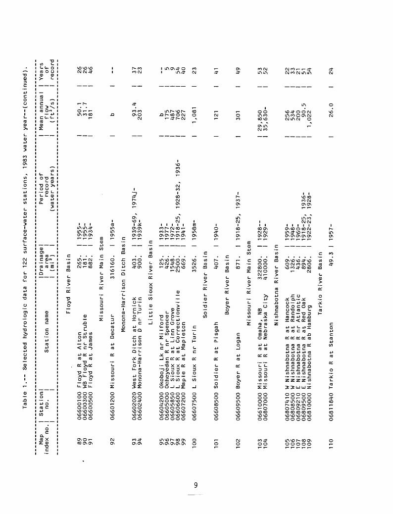
Table 1. Selected hydrologic data for 122 surface-waterstations, 1983 water year........................................... 6
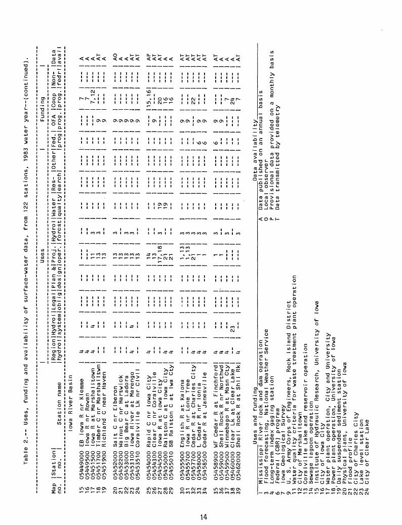
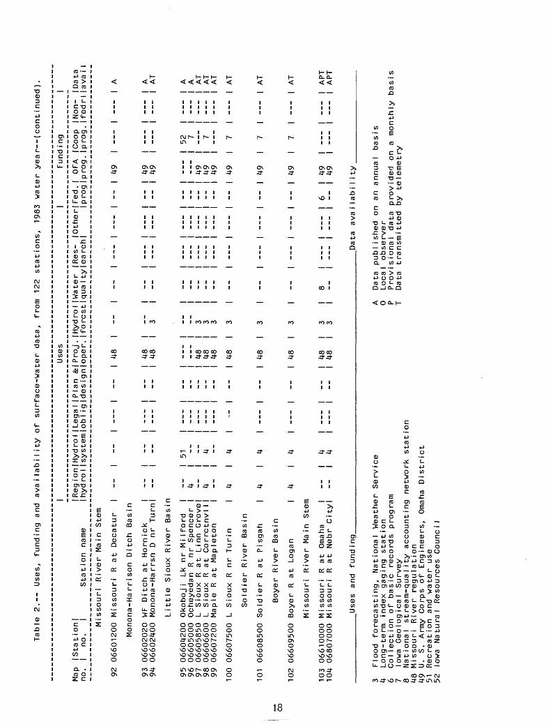
2. Uses, funding and availability of surface-water datafrom 122 stations, 1983 water year.................................. 13
3. Selected reach characteristics used in the flow- routing studies..................................... ................ 31
4. Summary of flow-routing results and comparisonbetween historic and simulated flows................................ 31
5. Summary of regression modeling results and comparisonbetween historic and simulated daily flows.......... ................ 32
6. Summary of the Kalman-filtering analysis.............. ............... 437. Summary of the routes that may be used to visit
stations in Iowa.................................... ................ 498. Selected results of K-CERA analysis................... ............... 50
IV

FACTORS FOR CONVERTING INCH-POUND TO METRIC (SI) UNITS
Multiply inch-pound units
foot (ft) mile (mi)
square mile (mi 2 )
cubic foot (ft 3 )
cubic foot per second (ftVs)
by
Length
0.30481.609
Area
2.590
Volume
0.02832
Flow
0.02832
To obtain SI units
meter (m) kilometer (km)
square kilometer (km 2 )
cubic meter (m 3 )
cubic meter per second (m 3 /s)

COST-EFFECTIVENESS OF THE STREAM-GAGING PROGRAM IN IOWA
By I. L. Burmeister, O. G. Lara
ABSTRACT
This report documents the results of a study of the cost-effectiveness of the stream-gaging program in Iowa. Data uses and funding sources were identified for the 122 surface-water stations (including reservoir, lake, stage only, and miscellaneous stations) operated by the U. S. Geological Survey in Iowa. There are 110 continuous streamflow stations currently being operated in Iowa with an annual budget of $592,000.
The average standard error of estimation in continuous streamflow records is 11.4 percent. It was shown that this overall degree of accuracy at the 110 continuous streamflow stations could be improved to 10.5 percent if the gaging schedule was optimized.
A minimum budget of $543,000 is required to operate the present stream- gaging program in Iowa. With this budget, routine visits to gages would be decreased to five during the open-water season and three during the winter. A budget less than this does not permit proper maintenance of the gages and recorders. At the minimum budget, the average standard error would be 12.5 percent. The maximum budget analyzed was $1,235,000, which resulted in an average standard error of 4.2 percent. A 10 percent increase in the current budget to $656,000 would result in a standard error of 8.4 percent.
There are still a few basins with drainage areas greater than 200 square miles that have no continuous streamflow data. Continuous streamflow gages need to be established in these basins as funds become available. All stations in the current program need to be maintained for the forseeable future.
Data simulated by using the flow-routing and regression methods for stations in 6 river basins do not meet the accuracy required for their data use. Other basins will be studied later to determine if alternative methods to meet accuracy standards are feasible.

INTRODUCTION
The U.S. Geological Survey is the principal Federal agency collecting surface- water data in the Nation. The data are collected in cooperation with State and local governments and other Federal agencies. The Geological Survey presently (1983) is operating approximately 8,000 continuous-record gaging stations throughout the Nation. Some of these records extend back to the turn of the century. Any activity of long standing, such as the collection of surface-water data, needs to be reexamined at intervals, if not continuously, because of changes in objectives, technology, or external constraints. The last systematic nationwide evaluation of the streamflow-information program was completed in 1970 and is documented by Benson and Carter (1973). The Geological Survey presently (1983) is undertaking another nationwide analysis of the stream-gaging program that will be completed in 5 years with 20 percent of the program being analyzed each year. The objective of this analysis and report is to define and document the most cost-effective means of obtaining and providing streamflow information.
For every continuous-record gaging station, the first phase of the analysis identifies the principal uses of the data and relates these uses to funding sources. Gaged sites for which data are no longer needed are identified, as are deficient or unmet data demands. In addition, gaging stations are categorized as to whether the data are available to users in a real-time sense, on a provisional basis, or at the end of the water year.
The second phase of the analysis is to identify less costly alternate methods of obtaining and providing the needed information; among these are flow-routing models and statistical methods. The stream-gaging activity no longer is considered just a network of measuring points, but rather an integrated information system in which data are provided both by measurements and synthesis.
The final phase of the analysis involves the use of Kalman-filtering and mathematical-programing techniques to define strategies for operation of the necessary stations that minimize the uncertainty in the streamflow records for given operating budgets. Kalman-filtering techniques are used to compute uncertainty functions (relating the standard errors of computation or estimation of streamflow records to the frequencies of visits to the stream gages) for all stations in the analysis. A steepest descent optimization program uses these uncertainty functions, information on practical stream-gaging routes, the various costs associated with stream gaging, and the total operating budget to identify the visit frequency for each station that minimizes the overall uncertainty in the streamflow records. The stream-gaging program that results from this analysis will meet the expressed water-data needs in the most cost-effective manner.
This report is organized into five sections; the first being an introduction to the stream-gaging activities in Iowa and to the study itself. The middle three sections each contain discussions of an individual phase of the analysis. Because of the sequential nature of the phases and the dependence of subsequent phases on the previous results, summaries are made at the end of each of the middle three sections. The study, including all phase summaries, is summarized in the final section.

150
1870
1880
18
90
19
00
1910
19
20
19
30
1940
19
50
19
60
1970
19
80
1990
Fig
ure
1.-
-His
tory
of
continuous s
tream
ga
gin
g i
n
Iow
a,
1873-1
983.
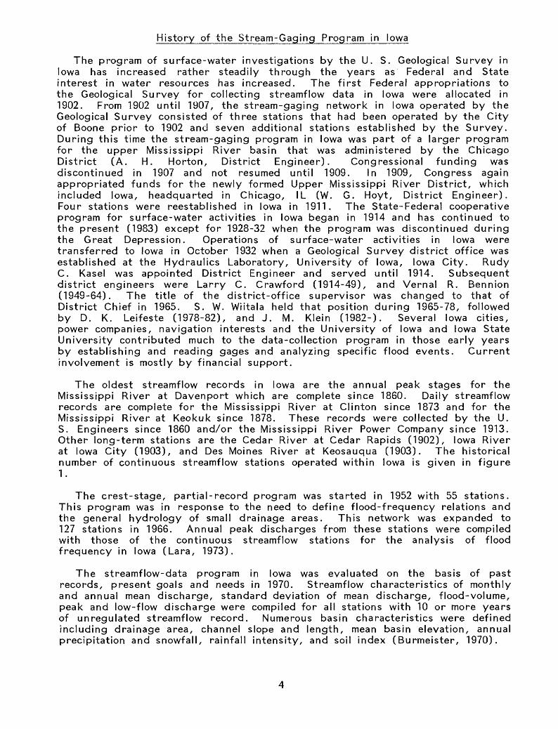
History of the Stream-Gaging Program in Iowa
The program of surface-water investigations by the U. S. Geological Survey in Iowa has increased rather steadily through the years as Federal and State interest in water resources has increased. The first Federal appropriations to the Geological Survey for collecting streamflow data in Iowa were allocated in 1902. From 1902 until 1907, the stream-gaging network in Iowa operated by the Geological Survey consisted of three stations that had been operated by the City of Boone prior to 1902 and seven additional stations established by the Survey. During this time the stream-gaging program in Iowa was part of a larger program for the upper Mississippi River basin that was administered by the Chicago District (A. H. Norton, District Engineer). Congressional funding was discontinued in 1907 and not resumed until 1909. In 1909, Congress again appropriated funds for the newly formed Upper Mississippi River District, which included Iowa, headquarted in Chicago, IL (W. G. Hoyt, District Engineer). Four stations were reestablished in Iowa in 1911. The State-Federal cooperative program for surface-water activities in Iowa began in 1914 and has continued to the present (1983) except for 1928-32 when the program was discontinued during the Great Depression. Operations of surface-water activities in Iowa were transferred to Iowa in October 1932 when a Geological Survey district office was established at the Hydraulics Laboratory, University of Iowa, Iowa City. Rudy C. Kasel was appointed District Engineer and served until 1914. Subsequent district engineers were Larry C. Crawford (1914-49), and Vernal R. Bennion (1949-64). The title of the district-office supervisor was changed to that of District Chief in 1965. S. W. Wiitala held that position during 1965-78, followed by D. K. Leifeste (1978-82), and J. M. Klein (1982-). Several Iowa cities, power companies, navigation interests and the University of Iowa and Iowa State University contributed much to the data-collection program in those early years by establishing and reading gages and analyzing specific flood events. Current involvement is mostly by financial support.
The oldest streamflow records in Iowa are the annual peak stages for the Mississippi River at Davenport which are complete since 1860. Daily streamflow records are complete for the Mississippi River at Clinton since 1873 and for the Mississippi River at Keokuk since 1878. These records were collected by the U. S. Engineers since 1860 and/or the Mississippi River Power Company since 1913. Other long-term stations are the Cedar River at Cedar Rapids (1902), Iowa River at Iowa City (1903), and Des Moines River at Keosauqua (1903). The historical number of continuous streamflow stations operated within Iowa is given in figure 1.
The crest-stage, partial-record program was started in 1952 with 55 stations. This program was in response to the need to define flood-frequency relations and the general hydrology of small drainage areas. This network was expanded to 127 stations in 1966. Annual peak discharges from these stations were compiled with those of the continuous streamflow stations for the analysis of flood frequency in Iowa (Lara, 1973).
The streamflow-data program in Iowa was evaluated on the basis of past records, present goals and needs in 1970. Streamflow characteristics of monthly and annual mean discharge, standard deviation of mean discharge, flood-volume, peak and low-flow discharge were compiled for all stations with 10 or more years of unregulated streamflow record. Numerous basin characteristics were defined including drainage area, channel slope and length, mean basin elevation, annual precipitation and snowfall, rainfall intensity, and soil index (Burmeister, 1970).

Fig
ure
2. L
oca
tion o
f st
ream
gag
es,
Dis
tric
t of
fice
, fi
eld
head
quar
ters
and
are
as o
f re
spon
sibi
lity
.

Table
1.--
Selected hy
drol
ogic
data fo
r 122
surface-water
stations,
1983 water ye
ar.
cr>
Map
index
no.
I St
atio
nl
I no
. I
I I
Station
name
I Dra ina
ge |
1 a re
a I
1 (m
i2
) |
Peri
od of
|
reco
rd
| (w
ater
ye
ars)
|
Mean annua
I fl
ow
(ft
s/s)
I Yea rs
I of
I
record
Upper
Iowa
River
Basin
1 2 3
05387490
05387500
0538
8250
Dry
Run
at Deco
rah
Upper
Iowa R
at Decorah
Upper
Iowa
R
nr Do
rche
ster
21.
I 511.
I 770.
I
1973
a-
| 1951-
I 1936-75a,
1975
- I
a 306
453
I I 30
I
6
Mississippi
Rive
r Ma
in St
em
4 5 6 7 8 9
0538
9500
05
4115
00
0541
1600
05
4125
00
0541
8450
05
4185
00
Miss
issi
ppi
R at McGregor
Miss
issi
ppi
R at Cl
ayto
n
Turk
ey
Turk
ey R
at Spillville
Turk
ey R
at Garber
Maquoketa
NF Maquoketa
R at Fu
lton
Maquoketa
R nr
Ma
quok
eta
6750
0.
I 79
200.
I
Rive
r Ba
sin
177.
I 15
45.
1
River
Basin
516.
1 15
53.
I
1936-
, 1
1975
a-
|
1956
-73,
19
77-
1 1913-16,1918-27,1929-30,1932-1
1977-
I 1913-
I
33,760
b 113
917
351
1,202
I 45
I 21
I 61
I 5
I 68
10 11 12 13 14 15 16 17 18 19 20 21 22 23 24
Mississippi
R i ve r
Ma i n
Stem
0542
0500
Mississippi
R at Cl
into
n 85
600.
I 18
73-
Wapsipinicon Ri
ver
Basin
0542
0560
Wa
psip
in icon
R nr
El ma
05421000 Wapsipinicon R
at Independence
0542
2000
Wa
psip
inic
on R
nr De
Witt
95.2
I 19
58-
1048
. I 1933-
2330.
I 19
34-
Crow
Cr
eek
Basin
0542
2470
Crow C
at Bett
endo
rf17
.8
I 19
77-
I 47,130 60
.5593
1,477 16.1
Iowa
R
i ve r
Ba s i n
05449000 EB
Io
wa R
nr Kl
emme
05
4495
00 Io
wa R
nr Rowan
0545
1500
Io
wa R
at Ma
rshal
I tow
n 05
4517
00 Ti
mber
C
nr Marshal
I tow
n 05451900 Rich I and
C ne
ar Ha
ven
0545
2000
Salt C
nr Elbe
ron
0545
2200
Wa
lnut
C
nr Hart
wick
05
4530
00 Bi
g Be
ar C
at La
dora
05
4531
00 Iowa Ri
ver
at Marengo
0545
3510
Coralville Lk
nr Co
ralv
ille
133.
429.
1564
.118. 56.1
201. 70.9
189.
2794.
3115.
1948
-76,
1940-76,
1902-03,
1949
-1949-
1945-
1949-
1945-
1956
-19
58-
1977-
1977-
1914-27,
1932
-
I 108 23 48 47
1
59.
196
770 66.
33.
122 41.
116
,662 c
3 6 3 3
32 40 63 32 32 36 32 36 25 --

Table
1.
Sele
cte
d
hyd
rolo
gic
d
ata
fo
r 12
2 su
rfa
ce
-wa
ter
sta
tions,
1983
w
ate
r year
(continued).
Map
index
no.
25
26
27
28
29 30
31
32
33
34 35
36
37
38
39 40
41
42
43
44 45 46
47
48
49
50
I Station!
j no.
| St
atio
n name
I I
I owa
R
i ve r
Ba s i n
05454000 Ra
pid
C nr Io
wa Ci
ty
0545
4300
Clear
C nr Co
ralv
ille
05
4545
00 Io
wa R
at Io
wa City
0545
5000
Ralston
C at Iowa City
0545
5010
S
BR Ra
lsto
n C
at Iowa City
05455500 English
R at
Ka
lona
05
4557
00 Io
wa R
nr Lo
ne Tr
ee
05457700 Ce
dar
R at
Charles
City
05458000 L Cedar
R nr Io
nia
05458500 Ce
dar
R at
Janesville
0545
8900
WF Cedar
R at Finchford
05459000 Sh
ell
Rock
R
nr No
rthw
ood
0545
9500
Winnegago
R at Mason
City
05460000 Cl
ear
Lk at Clear
Lake
05462000 Sh
ell
Rock
R
at Shell
Rock
05463000 Be
aver
C
at Ne
w Hartford
05463500 Bl
ack
Hawk
C
at Hu
dson
05464000 Cedar
R at
Wa
terl
oo
05464500 Cedar
R at Ce
dar
Rapi
ds
05465000 Cedar
R nr Co
nesv
ille
0546
5500
Io
wa R
at Wapello
Skunk
Rive
05470000 S Sk
unk
R nr Am
es
05470500 Sq
uaw
C at Am
es
05471500 S
Skun
k R
nr Os
kalo
osa
05472500 N
Skun
k R
nr Sigourney
05473400 Cedar
C nr Oa
klan
d Mills
I Dra
inag
e |
Peri
od of
Mean
annual
Year
s I
area
| re
cord
flow
of
I (m
i2
) (w
ater
ye
ars)
(f
t3/s)
record
-- Continued
25.3
1937-
15.3
44
98.1
1952
- 62.5
29
3271
. 1903-
1,64
1 78
3.0
1924-
1.69
57
2.9
1963-
2.42
18
573.
1939
- 35
9 42
4293.
1956-
2,668
25
1054.
1964
- 669
17
306.
19
54-
160
27
1661.
1904-06,1914-27,1932-42,1945-
806
61
846.
1945-
462
36
300.
19
45-
145
36
526.
1932-
245
49
22.6
1933-
b 1746.
1953-
900
28
347.
1945-
186
36
303.
19
52-
159
29
5146
. 19
40-
2,835
41
6510
. 1902-
3,305
79
7785.
1939-
4,463
42
1249
9.
I 1914-
6,716
67
r Ba s i n
315.
I 19
20-2
7, 1932-
150
56
204.
I 1919-27, 1965--
116
24
1635.
I 1945-
865
36
730.
I 1945-
420
36
522.
| 1957-77d,
1977-
410
5
51 52 53 54 55 56 57
05474000 Skunk R
at Augusta Mi ssi
ssipp
05474500 Mississippi R
at Keokuk
4303.
I 19
13,
1914-
River Ma in
Stem
1190
00.
I 18
78-
Des
Moines River Basin
05476500 De
s Moines R
at Estherville
1372.
05476750 Des
Moines R
at Humboldt
2256.
05479000 EF De
s Moines R
at Dakota City
1308.
05480500 De
s Moines R
at Fo
rt Dodge
4190
.05481000 Boone R
nr Webster City
844.
1951-
1964-
1940e-
1905-06, 19
13-2
7, 19
46-
1940f-
I 2,345
I 62,640
301
748
493
1,379
375
67
I 103 30 17 41 49 41

Ta
ble
1
.--
Sele
cte
d
hydro
logic
d
ata
fo
r 12
2 surf
ace-w
ate
r sta
tio
ns,
1983
w
ate
r year-
-(continued).
Map
in
dex
no
.S
tat
ion
I n
o.
| I
I Dra
in
ag
e |
Sta
tio
n
nam
e |
are
a
I I
(mi
2)
I
Period
of
reco
rd
(wate
r years
)
I M
ean
annua I
I flow
I
(ftV
s)
I Y
ea r
s
I o
f I
reco
rd
00
Des
Moi
nes
River
Basin
-- Continued
58
* 05
4813
00 De
s Mo
ines
R
nr Stratford
59
0548
1605
Bi
g C
pump
sta
nr Po
lk Ci
ty60
05481630 Sa
ylor
vill
e Lk nr
Sa
ylor
viIl
e61
05
4816
50 De
s Mo
ines
R
nr Sa
ylor
vill
e62
05
4819
50 Be
aver
C
nr Grim
es
63
0548
2135
N
Raccoon
R nr
Ne
well
64
05482170 Bi
g Ce
dar
C nr Va
rina
65
05482300 N
Raccoon
R nr
Sa
c Ci
ty66
0548
2315
Bl
ackh
awk
Lk nr
Lake Vi
ew67
0548
2500
N
Raccoon
R nr Je
ffer
son
68
0548
3000
EF Ha
rdin
C
nr Ch
urda
n69
0548
3450
M
Raccoon
R nr Ba
yard
70
05483470 Lake Panorama nr
Pa
nora
71
0548
3600
M
Raccoon
R at Pa
nora
72
05484000 S
Raccoon
R at Redfield
73
05484500 Raccoon
R at Va
n Me
ter
74
05484800 Wa
lnut
C
at Des
Moin
es75
0548
5500
De
s Mo
ines
R
bl Ra
c R
at Ds
m76
05485640 Fo
urmi
le C
at De
s Mo
ines
77
05486000 North
R nr Norwalk
78
05486490 Mi
ddle
R
nr Indianola
79
0548
7470
South
R nr Ackworth
80
05487980 Wh
ite
Brea
st C
nr Da
llas
81
0548
8100
Lake Re
d Ro
ck nr
Pe
l la
82
0548
8500
De
s Mo
ines
R
nr Tracy
83
0548
9000
Ce
dar
C nr Buss
ey84
05489500 De
s Mo
ines
R
at Ottumwa
85
05490500 De
s Mo
ines
R
at Ke
osau
qua
Big S
ioux
River
Basin
86
06483500 Rock R
nr Rock Valley
1592
. I 19
48-
Mis
sour
i River
Main
St
em
87
0648
6000
Missouri R
at Sioux
City
31
4600
. I
1897
-
Perry Cre
ek Basin
88
0660
0000
Perry
C at Siou
x Ci
ty
65.1
I 19
45-6
9,19
81-
5452.
91.4
5823
.5841.
358.
217. 80.0
713. 23.3
1619.
24.0
375.
433.
440.
988.
3441
.80.9
9879
.92.7
349.
503.
460.
342.
12323.
12479.
374.
1337
4.14
038.
19209-
1978
-1977-
1961
-1960-
1982-
1959
-1958-
1970-75,1978-
1940
-
1952
-
1979-
1958-
1940
-
1915-
1971
-19
40-
1971-
1940
-
1940
1940-
1962-
1969-
1920
-
1947
-1917h-
1903-06, 1910,
1911
1,780 b c
2,44
718
8 35.5
287 b
658 9.
31
b20
1435
1,284 58.8
4,021 63.7
173
247
235
155 c
4,64
1
197
5,068
3,217
61 -- -- 20 21 22 23 -- 41 29 __ 23 41 66 10 41 10 41 41 41 19 -- 61 34 64 72
316
I 32,030 14.7
33 84 25
Table
1.-
- S
ele
cte
d
hyd
rolo
gic
d
ata
fo
r 12
2 su
rfa
ce
-wa
ter
sta
tio
ns,
1983
w
ate
r ye
ar-
-(co
ntin
ue
d).
Map
inde
x no.
89
90
91 92
1 St
atio
n!
I no
. |
Stat
ion
name
1
1
F 1 oyd
0660
0100
Floyd
R at Al
ton
0660
0300
WB Floyd
R nr
Struble
0660
0500
Floyd
R at
Ja
mes
Mi ssouri
0660
1200
Missouri R
at Decatur
|Dra
inag
e|
Peri
od of
I area
| re
cord
1
(mi
2)
(wat
er ye
ars)
R i ve r
Ba s i n
265.
1 19
55-
181.
19
55-
882.
1934-
Rive
r Ma in
Stem
316160.
1955
a-
I Mean annua
1 I
flow
1 (ftVs)
1 50
.1
1 31
.7
181 b
Yea rs
1
of
reco
rd
26
26
46 --
Mono
na-H
arri
son
Ditc
h Basin
93
9406
6020
20 We
st Fo
rk Ditch
at Hornick
0660
2400
Monona-Harrison D
nr Turin
403.
1939
-69,
19
74J-
900.
1939
k-93.4
203
37
23
Litt
le Si
oux
Rive
r Ba
sin
95
96
97
98
99 100
0660
4200
Okoboj i
Lk nr Mil ford
125.
1933
- 06
6050
00 Oc
heye
dan
R nr
Sp
ence
r 426.
1977-
0660
5850
L
Sioux
R at
Linn Grove
1548
. 19
72-
0660
6600
L
Sioux
R at Correct ionvi
1 le
2500.
1918-25, 1928-32, 19
36-
0660
7200
Maple
R at
Mapleton
669.
1941
-
0660
7500
L Sioux
R nr Tu
rin
3526
. 19
58m-
b 175
487
706
227
1,08
1
5 9 54
40 23
So 1 d
i e r R
i ve r
Ba s i n
101
102
103
104
0660
8500
So
ldie
r R
at Pi
sgah
Boyer
0660
9500
Bo
yer
R at
Lo
gan
Mi ssouri
0661
0000
Missouri R
at Om
aha,
NB
0680
7000
Missouri R
at Ne
bras
ka Ci
ty
407.
1940-
R i ve r
Ba s i n
871.
1918
-25,
19
37-
River
Ma in
Stem
3228
00.
1928--
410000.
1929-
121
301
29,8
50
35,6
30-
41 49 53
52
Nishnabotna
Rive
r Basin
105
106
107
108
109
0680
7410
W
Nish
nabo
tna
R at Ha
ncoc
k 06
8085
00 W
Nishnabotna
R at Randolph
0680
9210
E Ni
shna
botn
a R
nr At
lant
ic
0680
9500
E
Nishnabotna
R at Red
Oak
0681
0000
Nishnabotna
R ab Hamburg
609.
1959
- 1326.
1948-
436.
1960
- 89
4.
1918
-25,
1936-
2806
. 1922-23, 1928-
256
534
200 90.5
1,022
22 33
21
51
54
110
0681
1840
Ta
rkio
R
at Stanton
Tark
io Ri
ver
Basi
n
49.3
I 1957-
26.0
24

Table
1.-- Se
lect
ed hy
drol
ogic
data fo
r 122
surface-water
stat
ions
, 1983 water ye
ar--
(con
tinu
ed).
Map
|index
no.
| 1
Stat
ion
no.
Stat
ion
I Dra inage |
name
| ar
ea
I1
(mi
2)
|
Peri
od of
reco
rd(w
ater
ye
ars)
Mean
annua
1flow
(ftVs)
I Yea rs
1 of
I re
cord
111
112
113
115
116
117
118
119
120
121
122
Missouri River
Main
St
em
06813500 Missouri R
at Ru
lo,
NB
414900.
I 1949-
Noda
way
River
Basin
0681
7000
No
dawa
y R
at Clarinda
762.
| 1918-25, 19
36-
Plat
te Ri
ver
Basi
n
0681
8750
Platte R
nr Diagonal
06819190 EF 102
R nr
Bedford
217.
I 1968-
92.1
| 1959-
Grand
River
Basi
n
0689
7950
Elk
C nr
Decatur Ci
ty06
8980
00 Thompson R
at Davis
City
0689
8400
We I don
R nr Leon
52.5
701
.104.
Char
iton
Ri
ver
Basi
n
0690
3400
Chariton R
nr Ch
arit
on
182.
0690
3700
SF
Ch
arit
on R
nr Promise
City
16
8.06
9039
00 Rathbun
Lk nr
Rathbun
549.
0690
3900
Ch
arit
on R
nr Rathbun
549.
0690
4010
Ch
arit
on R
nr Mo
ulto
n 740.
1967-
1918
-25,
1958-
1965n-
1967p-
1969
-1956-
1979
-
1941-
I 39
,530 323
I 117
I 50.7
28.4
361 72
.0
104
109 c 318
679
32 51 13 22 14 46 23 16 14 253
FOOT
NOTE
S:
a b c d e f
s i te.
"at
Hard
y".
to September
1927.
Oper
ated
as mi
scel
lane
ous
site
.Stag
e,
in fe
et,
only
.Cont
ents
, in
ac
re-f
t, on
ly.
Oper
ated
as
low-flow part ia I-record
Prior
to Oc
tobe
r 19
54.
publis
hed
asPublished
as "a
t Kalo"
October 1913
g Published
as "near
Boon
e" 19
20-67.
h Published
as "a
t Eldon" October 1930 to Ma
rch
1935
. j
Published
as "a
t Holly
Spring
s" Ap
ril
1939 to September 19
69.
k Re
cord
s fo
r Ap
ril
1939
to January 19
58 no
t equivalent.
Prior
toMa
y 19
42,
published
as "near
Blencoe".
m Publ
ished
as "near
Blencoe"
Ap
ril
1939 to Ma
y 1942 at
site 4.
7 mi
les
down
stre
am.
Reco
rds
not
equi
vale
nt April
1939 to January 1958.
n Oc
casi
onal
low-flow measurements 19
58-6
0, 19
62,
1964.
p Oc
casional lo
w-fl
ow measurements 19
58-6
6.
Publ
ishe
d as "near
Bethlehem'
1958-66.

Current Stream-Gaging Program in Iowa
During 1983, 110 continuous streamflow stations, 126 crest-stage gages, and 4 stage-only or miscellaneous stations were operated by the U. S. Geological Survey in Iowa. Of these stations, only the 110 continuous streamflow stations (fig. 2, table 1) were included in all three phases of the analysis. The cost of operating the 110 continuous streamflow stations during 1983 was $592,000.
The 126 crest-stage gages, the 4 stage-only or miscellaneous stations, 4 lake- stage stations, 11 continuous daily water-quality stations, and 43 ground-water observation wells were included only in the third phase of the analysis because the activities associated with operating, measuring, and maintaining these stations and wells are included in the hydrographers' work schedules when they visit the 110 continuous streamflow stations.
In addition to data for the 110 continuous streamflow stations in table 1, data for the 4 stage-only and miscellaneous stations, the 4 lake-stage stations, and the 4 reservoir-content stations also are included in table 1 because they are included routinely in the hydrographers 1 work schedules. The location of the additional 12 stations also is shown in figure 2.
The responsibility for data collection and records computation for the 110 continuous streamflow stations and the other 12 stations is shared by the District office at Iowa City and the Field-Headquarters offices at Fort Dodge and Council Bluffs. The strategic location of each office decreases time and travel to the stations for which the offices are responsible, and consequently increases the opportunity to measure peak discharges during floods and to define the stage- discharge relationship at each station. The location of these offices and the assigned area of responsibility are shown in figure 2. Table 1 also provides the official U. S. Geological Survey eight-digit downstream-order station number, and name of each station.
USES, FUNDING, AND AVAILABILITY OF CONTINUOUS STREAMFLOW DATA
The relevance of a stream gage is defined by the uses that are made of the data that are produced from the gage. The uses of the data from each gage in the Iowa program were identified by a survey of known data users. The survey documented the importance of each gage and identified gaging stations that may be considered for discontinuation.
Data uses identified by the survey were categorized into nine classes, definedbelow. The sources of funding for each gage and the frequency at which dataare provided to the users also were compiled (table 2).
Data-Use Classes
The following definitions were used to categorize each known use of streamflow data for each continuous stream gage:
11

Regional Hydrology
For data to be useful in defining regional hydrology, a gaged stream needs to be largely unaffected by manmade storage or diversion. In this class of uses, the effects of man on streamflow are not necessarily small, but the effects are limited to those caused primarily by land-use and climate changes. Large volumes of manmade storage may exist in the basin providing the outflow is uncontrolled. These stations are useful in developing regionally transferable information about the relationship between basin characteristics and streamflow.
Sixty-four stations in the Iowa network are classified in the regional hydrology data-use category. Four of the stations are special cases in that they are designated bench-mark or index stations. There is one hydrologic bench mark station in Iowa, Elk Creek near Decatur City (06897950), which is used to indicate hydrologic conditions in watersheds relatively free of manmade alteration. Three index stations are used to indicate current hydrologic conditions for a national monthly summary. They are the Cedar River at Cedar Rapids (05464500), Des Moines River at Fort Dodge (05480500), and Nishnabotna River above Hamburg (06810000). Twelve stations are not funded for other uses. When sufficient hydrologic data are available to define the hydrologic characteristics of the basin, each of these stations will be considered for discontinuance. None are candidates at this time.
Hydrologic Systems
Stations that can be used for accounting, that is, to define current hydrologic conditions and the sources, sinks, and fluxes of water through hydrologic systems including regulated systems, are designated as hydrologic-systems stations. They include diversions and return flows and stations that are useful for defining the interaction of water systems.
Forty-four streamflow stations in the Iowa network are classified in the hydrologic-systems category including the 4 bench-mark and index stations. They are used to account for the current and long-term conditions of the hydrologic systems that they gage.
Legal Obligations
Some stations provide records of flows for the verification or enforcement of existing treaties, compacts, and decrees. The legal-obligation category contains only those stations that the U. S. Geological Survey is required to operate to fulfill a legal responsibility. There are no stations in the Iowa program that exist to fulfill a legal responsibility of the Geological Survey.
Planning and Design
Gaging stations in this category of data use are used for the planning and design of a specific project or group of structures. For example, streamflow data are needed for the design of dams, reservoir storage, flood control, levees, floodwalls, navigation systems, water supplies, hydropower plants, or waste- treatment facilities. The planning- and design-category is limited to those stations that were instituted for such purposes and where this purpose is still valid. Currently, no stations in the Iowa program are being operated for planning- or design-purposes but data from several stations were used in the past for the design of large reservoirs and flood walls.
12

Table
2.
Use
s,
fun
din
g
and a
va
ila
bility o
f surf
ace-w
ate
r data
, fr
om
12
2 sta
tio
ns,
19
83
w
ate
r ye
ar.
Map
n
o.
1 2 3 4 5 6 7 8 Q
I Sta
tio
n I
I n
o.
|
05387490
05
38
75
00
0
53
88
25
0 Mi
05
38
95
00
05411500
05
41
16
00
0
54
12
50
0
05418450
n^i
iift^
nn.
1U
ses
| F
undin
g
|
|Reg
ionlH
ydro
l | L
ega
1 | P
lan
&| P
roj. i
Hydro
l IW
ate
r |R
es-
|Oth
er|
Fe
d.|
OFA
|C
oop
|No
n-
IDa
ta
Sta
t io
n
nam
e | h
ydro
1 j s
yste
m jo
b 1
ig |
de
sig
n jo p
er.
| fo
rest
I qua
1 ty
lea r
ch
j Ip
rog
j p
rog
. | p
rog
, j f
ed
rl J
ava
i 1
Upper
Iow
a R
iver
Basin
Dry
R
un a
t D
eco
rah
| U
pper
Iow
a R
at
De
cora
h|
Up
pe
r Io
wa
R nr
Drc
hstr
j
ssis
sip
pi
Riv
er
Main
S
tem
Mis
sis
sip
pi
R a
t M
cGrg
rl
Mis
sis
sip
pi
R a
t C
laytn
j
Turk
ey R
iver
Basin
Turk
ey
R a
t S
pillv
ille
|
Turk
ey
R a
t G
arb
er
|
Maquoke
ta
Riv
er
Basin
NF
Ma
qu
oke
ta
R a
t F
ultn
lM
am
in U
P -
i- a
R
n r
- M
annnU
l-a
1
1
\
1 1
I
I
I
I
I
2 |
|
| A
4
I
I
I
I
I 3
I
I
I
I 6
I
I
I AO
"
I
I
I
I 1
I 3
I
I
I
I --
2
I
|
| A
T
4 I
I
I
I 1
I
I 5
I
I
I 6
I 2
|
|
| A
__
I --
I _
__
__
1 1
__
__
________
Q
1 _..
__
AT
1
1 1
I'l
1 1
1 1
1 <-
1
1 1
A 1
ii
1 __
1 _
__
1
__
1 _
__
1
__
I __
1 _
__
1
__
_
1 __
1 _
__
I
7
1 _
__
1
A
l,
1 II
1
j 1
7
1 j
1 II
1 T
1
1 A
TH
I
H
| |
| |O
|
I I
I I
1 I
1
1 A
1
1.
1 __
I _
__
|
__
| _
__
I
__
| __
| _
__
I
__
_
I __
1 _
_
1 7
1
__
1 A
HI
||
||
| 1
1 1
1 1
1 \
1 A
il
1 il
1 -
1 --
1 --- 17
1 --
1 ---
1 -
1 --
1 _
--
1 7
1
--_
1
AT
Mississippi
River
Main St
em
10
0542
0500
Mississippi
R at Clintnl
Wa p s i p
i n i co
n R
i ve r
Ba s i n
11
0542
0560
Wapsipinicon R
nr El
ma
|12
05
4210
00 Wa
psip
inic
on R
at Indndj
13
0542
2000
Wapsipinicon R
nr Dewtt|
Crow
Cr
eek
Basin
14
0542
2470
Crow C
at Bettendorf
___________Uses and
fund
ing
I 4
I
II
1 I
18
I
I
1 6
1 9
1
1 A
tun
a
| H
|
| -
| --
|
---
| ;
Indndl
4 I
4 I
I --
I
I 3
D
ew
tt |
4 I
4 I
I --
I
1 |
3
sin
ion
i --
i
-- ll
II
I dam
opera
tion
irs,
St.
P
au
l D
istr
ict
We
ath
er
Se
rvic
e
ion
i I I A
0 P T
-- --
i
i -
i I
I
II
I
I
I 10
|
I
Da
ta
ava
i
Data
p
ub
I is
hed
on
Loca
I observ
er
Pro
v i s
io
na
I d
ata
D
ata
tr
ansm
itte
d
--
1 9
1 9
1 a b
i 1
i ty
an
annua
pro
vid
ed
by
te le
me
i i
i --
- 1
7 1
I
|
i __
_ i
___
1 bas
i s
on
a m
on
thly
tr
y
1 A
1 A
T
1 A
T
1 A
bas
i sLong
-ter
m index
gagi
ng st
atio
nU.
S. Army Co
rps
of En
gine
ers
GREAT
I sedimentation
stud
yCo
llec
tion
of
basic
reco
rds
program
Iowa
Geological Su
rvey
National st
ream
-qua
lity
accounting network
stat
ion
U.
S. Army Corps
of En
gine
ers,
Rock Island District
10 Urbanization st
udy
Ta
ble
2.-
- U
ses,
fu
nd
ing
and availability o
f su
rfa
ce
-wa
ter
da
ta,
fro
m
122
sta
tion
s,
1983
w
ate
r year-
-(continued).
Map
no.
ISta
t io
nl
I no.
I
IUses
I Reg ion
| Hy
dro
I | Lega
I | Plan
&| Proj
. St
atio
n name
| hyd
ro I
| sys
temj
obl
ig jdes ign joper.
I Funding
|
I Hydro I
| Water |R
es-
|Other|Fed.
I for
est
| qua I ty
|ea
rch |
I pro
gI OFA
I prog.
I Coo
p I pro
g.iN
on-
Ifedrl
I Dat
a la
va i
I
Iow
a R
ive
r B
asin
15 16 17 18 19 20 21 22 23 24 25 26 27 28 29 30 31 32 33 34 35 36 37 38 39
05449000
0544
9500
0545
1500
0545
1700
0545
1900
0545
2000
0545
2200
0545
3000
05453100
0545
3510
0545
4000
05454300
0545
4500
0545
5000
0545
5010
05455500
05455700
0545
7700
05458000
05458500
0545
8900
0545
9000
05459500
0546
0000
0546
2000
EB Io
wa R
nr Kl
emme
Iowa R
nr Rowan
Iowa
R
at Ma
rsha
l I town
Timber C
nr Ma
rsha
lltw
nRich
land C
near Haven
Sa 1
1 C
nr Elberon
Walnut C
nr Hartwick
Big
Bea
r C
at Ladora
Iowa River at
Marengo
Co ra
I v i
I I e Lk n r Ci
vil
Ra p i d
C n r
I owa
C
i ty
Clear
C nr Co
ra I vi
Me
Iowa R
at Io
wa City
Ralston
C at
Iowa
Ci
tySB Ralston
C at
Iwa
Cty
Eng
I i sh
R at Ka lon
aIo
wa R
nr Lo
ne Tree
Cedar
R at
Charles
City
L Ce
da r R
nr Io
n ia
Cedar R
at Janesvi
I le
WF Cedar R
at Fi
nchf
ord
Shel
l Ro
ck R
nr Northwd
Winnebago R
at Masn Ct
yClear
Lk at Cl
ear
Lake
Shel
I Ro
ck R
at Sh
l I Rk
I 4 4 4 - - _ - - 4 - 4 - - 4 4 - - 4 4 4 4 4 4 4
4 -- -- __ -- -- 4 -- __ -- _- -- -- -- -- __ -- 3
___
___
---
___
___
___
___
---
___
___
~-_
___
___
___
---
___
__ -- -- __ -- -- -- -- __ -- -- -- -- -- -- __
i ---
11 13 13 13 13 13 13 13 14 1317
,18
21 21 1,13
1,13
211 1 1 1
i
3 3 -- 3 -- 3 3 -- __ -- 3 -- -- 3 3 3 3 3 3 3 3
-- --
__ -- -- -- -- 19 19 -- _-
-- __ --
___
---
___
___
---
---
---
---
___
---
___
---
i --
-
___
___
___
---
---
---
---
___
---
-- -- __ -- -- -- -- -- -- 6 6 6 --
9 9 9 9 9 9 9
9
9 9
9 9 9 9
i 77,1
2__
_--
-
___
___
---
___
---
15
,16
20 16 16 22 ---
___ 7
247
A A A AT
A AO
A A AT
AT
AP
AT
AT
A A AT
A
T
AT
A
T
AT
AT
A A A AT
I 3 4 6 7 9 11 12
13
__
__
__
__
_U
se
s
and
fun
din
g_
__
__
__
__
__
__
__
__
__
M
issis
sip
pi
Riv
er
lock
and
dam
opera
tion
Flo
od
fo
reca
stin
g,
Na
tio
na
l W
ea
the
r S
erv
ice
L
on
g-t
erm
in
de
x
gagin
g
sta
tio
n
Federa
l (C
BR
) p
rog
ram
Io
wa
Ge
olo
gic
al
Surv
ey
U.
S.
Arm
y C
orp
s o
f E
ngin
eers
, R
ock
Is
lan
d D
istr
ict
_Data
ava
i la
b i
I i ty_
Water qu
alit
y cr
iter
ia fo
r wa
ste
treatment
plant
oper
atio
nCity
of
Ma
rshal
I town
Cora I vi
Me La
ke and
reservoir
operatio
n14
Sewage lagoon
op
erat
ion
15 In
stit
ute
of Hy
drau
lic
Rese
arch
, University of
Io
wa16 City
of
Iowa Ci
ty17 Water
plant
oper
atio
n, City and
University
18j Powe
r plant
oper
atio
n, Un
iver
sity
of Iowa
19'Dai
ly suspended
sedi
ment
station
20 Physical plant, University of Io
wa21 Fl
ood
prof
ile
22 City
of Charles
City
23 Lake level
station
24 City
of
Clear
Lake
A Data publ
ishe
d on an
annual basis
0 Lo
ca I
observer
P Pr
ovis
iona
l da
ta provided on a
monthly ba
sis
T Data tr
ansmitted
by telemetry

Table 2. Us
es,
funding
and
availability of surface-water da
ta,
from
122
stat
ions,
1983 water year (continued).
Map
| S
tation!
no
. |
no
. |
Sta
tio
n
nam
e
Iow
a R
ive
r B
asin
--
co
nt.
40
05
46
30
00
B
ea
ve
r C
at
New
H
art
frd
41
0
54
63
50
0
Bla
ck
Haw
k C
at
Hudso
n
42
05
46
40
00
C
edar
R a
t W
ate
rloo
43
05
46
45
00
C
edar
R a
t C
ed
ar
Ra
pid
s
44
0
54
65
00
0
Ce
da
r R
nr
Co
ne
svi
I le
45
05
46
55
00
Io
wa
R a
t W
apello
Sku
nk
Riv
er
Basin
46
05
47
00
00
S
Sku
nk
R n
r A
mes
47
0
54
70
50
0
Squ
aw
C a
t A
mes
48
0
54
71
50
0
S S
kun
k R
nr
Oskalo
osa
49
05472500
N S
kun
k R
nr
Sig
ou
rne
yR
n
r\K
li~
Til<
r\r\
ro
rtu
r- r
nr-
H
aLla
nH
M
l Ic
Use
s
Regio
n
Hyd
ro I
Legal
Plz
hydro
I sy
ste
m jo
b I
ig j
de
s
4 4 4
4 4
4 4
4 4
4 4 ......
in
&|
Pro
j. |
Hyd
ro I
| Wa
ter
Re
s-
|Oth
er|
F
sig
n
oper.
fo
rest
Iqua I
tyle
a r
ch
j |p
..1
3£
1
\J
1,2
1
3 -
126,2
7
3 -13
3 8
\J
..13
Fun
d in
g
"ed.
OFA
|C
oop
|No
n-
» rog |
p ro
g .
p ro
g .
| fed r
1
9
1
25
1
9 1
25
1
128,2
91
9
|
6
I
7 |
30,3
21
9
1
7 |
Data
ava
i 1
AT
AT
AT
AP
T
AT
AT
AT
A
OT
A
T
AT
AH
51
0547
4000
Skun
k R
at Augusta
| 4
Miss
issi
ppi
Rive
r Main Stem
52
0547
4500
Miss
issippi
R at
Ke
okuk
l 4
|I 8,19
I
I
AT
33
16
I
I 34
.Uses
and
funding.
.Dat
a av
aila
bili
ty.
I Mississippi
River lo
ck and
dam
operation
3 Flood
fore
cast
ing, National Weather Service
4 Long-term
index
gagi
ng station
6 Collection of ba
sic
reco
rds
prog
ram
7 Io
wa Geological
Survey
8 National stream-quality accounting ne
twork
station
9 U.
S. Ar
my Co
rps
of En
gine
ers,
Rock Island Di
stri
ctII Water
quality criteria fo
r wa
ste
trea
tmen
t plant
oper
atio
n 13 Coralville La
ke an
d reservoir
operation
19 Daily
susp
ende
d se
dime
nt station
21 Flood
prof i
le
City
of
Waterloo
Palo
nu
clea
r power plant
oper
atio
n Flood
profile
and
city
da
m op
erat
ion
Power
Co.
Rapi
ds
25 26 27 28 29 30 31 32 33 34
Iowa
Electric
City of
Ceda r
City of Am
esFlood
warning
Iowa State
University
Powe
r ge
nera
tion
Union
Elec
tric Power
Co.
A Da
ta pu
blished
on an an
nual
ba
sis
0 Loca I
observer
P Pr
ovis
ional
data provided on a monthly ba
sis
T Da
ta tr
ansmitted
by telemetry

Table
2.-- Us
es,
funding
and
availability of surface-water
data
, fr
om 122
stat
ions
, 1983 wa
ter year (continued).
Map
n
o.
|Sta
t io
n |
1 n
o.
|
1 I Reg
i o
n I
Hyd
ro 1
| Leg
a 1
Sta
t i
on
nam
e I h
yd r
o 1
I sys
tem
| ob
1 i g
Use
s
1 P 1
a n
& |
P ro
j .
|des ign joper.
1 F
undin
g
|
iHyd
rol
(Wa
ter
|Res-
|Oth
er|
Fed.|
OFA
(f
ore
st
Iqua Ity
learc
hl
Ipro
g I
pro
g.
iCo
op
Ip
rog.
iNo
n-
Ifedrl
(Da
ta
Java
i 1
Des Moi
nes
River
Basin
53
0547
6500
Des
Moin
es R
at EstrvlI
I54
0547
6750
Des
Moin
es R
at Humbldtl
55
0547
9000
EF
Des
Moin
es R
at Daktl
56
0548
0500
Des
Moin
es R
at Ft
DodgI
57
0548
1000
Boone
R nr W
ebst
er Ci
ty I
58
0548
1300
Des
Moin
es R
nr St
rtfr
d59
05
4816
05 Bi
g C
Sta
nr Polk City
60
0548
1650
Saylorville
Lk nr Sylvl
61
0548
1650
Des
Moin
es R
nr Sy
lorv
l62
0548
1950
Beaver C
nr Gr
imes
63
0548
2135
N
Racc
oon
R nr Newell
|64
0548
2170
Big
Ceda
r C
nr Va
rina
|
65
0548
2300
N
Racc
oon
R nr Sac
City I
66
0548
2315
Blackhawk
Lk at Lk Viewl
67
0548
2500
N
Racc
oon
R nr J
effersnj
68
0548
3000
EF
Ha
rdin
C
nr Ch
urda
n |
69
0548
3450
M
Racc
oon
R nr Ba
yard
|
70
0548
3470
Lake Pa
nora
ma nr Panora
71
0548
3600
M
Racc
oon
R at
Panora
72
0548
4000
S
Racc
oon
R at Redfield
-- -- -- 4 -- 4 __ -- -- 41 4 -- 4 4
___
___
___
---
-- -- -- __ «« -- _- -- -- __ -- -- --
___
35 3535,36
35 35 38 35 39 39 11 41 39
43
43 39
3 3 3 3 3 3 -- -_ -- 3 -- 3 -_ 3
-- -- _- -. _- 19 -- --
43
43 43--
___
-__
___
___
---
__.
___
_-._
-__
43
43 43 ---
___
___
___
--«
___
_-«
6 -- -- -- -- -- -- --
___ 9 9 9 9 9 9 9 9 9
_ -._
9 -__ 9
___
-.-.
____
37 ---
___
___
___
___
---
40 7 742 7 44
44 7 ---
AO
AO
ATAPT
AT
AT
AT
AT
AT
AT
AT
A A A AT
A AT
ATA AT
_Use
s and
fund
ing.
_Data
ava
i lab i
I i ty_
3 Fl
ood
fore
cast
ing,
Na
tion
al We
athe
r Se
rvic
e4
Long
-ter
m index
gagi
ng station
6 Collection of basic
reco
rds
prog
ram
7 Iowa Ge
oIog
i ca
I Su rvey
9 U.
S. Ar
my Co
rps
of Engineers, Ro
ck Is
land
Di
stri
ct11
Water
quality
criteria fo
r wa
ste
trea
tmen
t pl
ant
oper
atio
n35 Saylorville
Lake and
reservoir
operation
36 Street and
storm
sewer
oper
atio
n37 City of
Fo
rt Do
dge
38 Mo
nito
ring
de
tention
dam
oper
atio
n needs
39 Lake Red
Rock
re
serv
oir
oper
atio
n40 Iowa Be
ef Pa
cker
Co
.41
Mo
nito
r ef
fect
s of ground water
use
42 We
st Central
Iowa Rural
Water
Asso
ciat
ion
43 Sedimentation
study
of Lake Panorama
44 Central
Iowa Po
wer
Company
Data pu
blis
hed
on an annual basis
LocaI
obse
rver
Prov
isio
nal
data pr
ovid
ed on a
monthly
basi
sData transmitted
by te
leme
try

Table
2.-
- U
ses,
fu
ndin
g
and
availability o
f surf
ace-w
ate
r d
ata
, fr
om
12
2 sta
tio
ns,
1983
w
ate
r year-
-(continued).
Map
| S
tatio
n |
no
. I
no
. I
Sta
tio
n
nam
e
Use
s
Reg
io
n
hyd
ro I
Hyd
ro I
syst
em
Lega
1 obi
igP
lan
&
Ide
s ig
nP
ro j
. o
pe
r.
Des
M
oin
es
Riv
er
Basin
co
nt.
7^
nR
tiR
ti^in
n
Rarr-oon
R
a 1
- W
an
Mtn
-o r
» '
'
__
_
__
Jir;
/ O
U
l/H
OH
I/U
U
rxdU
ULJU
il
r\
a L
. va
il llcto
i
74
0
54
84
80
0
Waln
ut
C a
t D
es
Mo
ine
s75
0
54
85
50
0
Des
M
oin
es
R B
l R
ac
R76
0
54
85
64
0
Fourm
ile
C a
t D
es
Moin
s77
0
54
86
00
0
Nort
h
R n
r N
orw
alk
78
05
48
64
90
M
idd
le
R n
r In
dia
no
la79
0
54
87
47
0
South
R
nr
Ackw
ort
h80
0
54
87
98
0
White
Bre
ast
C n
r Da
1 1 s
81
05
48
81
00
Lk
Red
R
ock
n
r P
el l
a8
2
05
48
85
00
D
es
Moin
es
R n
r T
racy
83
05
48
90
00
C
ed
ar
C nr
Bu
sse
y84
05
48
95
00
D
es
Moin
es
R a
t O
ttum
wa
85
05
49
05
00
D
es
Moin
es
R a
t K
eosq
ua
t -- -- -- -- __ -- --
t
^j 10
Hyd
ro 1
I Wa te
r
fore
st
1 qua
1 ty
Re
s-
(Oth
er
earc
hj
Fun
d i n
g
Fe
d.
pro
gO
FA
pro
g.
Coo
p I N
on
- p
rog
. | f
ed
rl
I Data
a
va i
I
3
_-
_-._
1
ll£
A
T
3,1
0
104
--
39
,45
! 3
10 39
_-
-- -- -- 4 4
___
___
___
___
---
___
___
4 1
__ -- -- -- -- __ -- --
39 39 39 39 39 39 39 39
3 3 3 3 3 -- 3 3 3
-_ -- -- -- -- __ --3
I
___
___
___
___
___
___
---
___
__
__
__
__
_---
___
__
_
-- -- -- -- 6
9 9 9 9 9 9 9 9 9 9
+U
47 47 47 ___
___
___
---
___
___
___
___
___
___
___
---
__..
AA
1
AO
AP
TA
OA
T
AT
AT
AT
AT
AT
AT
AT
AT
Big
S
ioux
Riv
er
Ba
sin
86
06483500
Rock
R
nr
Ro
ck V
alley
I 4
Mis
souri
Riv
er
Main
S
tem
87 88 89 90 91
06
48
60
00
M
issouri
R a
t S
ioux C
tyl
Pe
rry
Cre
ek
Basin
06600000
Pe
rry
C a
t S
iou
x C
ity
I
Flo
yd
R
iver
Ba
sin
06
60
01
00
F
loyd
R a
t A
lto
n
|0
66
00
30
0
WB
Flo
yd
R nr
St ru
ble
I
06
60
05
00
F
loyd
R
at
Jam
es
|
I 4
8
I 3
I 48
I
31
45
,48
1
3
49
I
104
9
I
I 49
I
I 49
I
I 49
50
AT
I 6
I 4
9
I
I
I A
PT
AO
I AT
I AO
I AT
Use
s an
d fu
nd
ing
_Data
ava
i lab
i I i
ty_
3 F
lood
fore
casting,
Na
tio
na
l W
eath
er
Se
rvic
e4
Lo
ng
-te
rm
index
gagin
g
sta
tio
n6
Co
lle
ctio
n o
f basic
re
cord
s
pro
gra
m7
Iow
a G
eo
log
ica
l S
urv
ey
8 N
atio
na
l str
ea
m-q
ua
lity
accounting
netw
ork
sta
tio
n9
U.
S.
Arm
y C
orp
s o
f E
ng
ine
ers
, R
ock
Is
land D
istr
ict
10
Urb
an
iza
tio
n
stu
dy
39
Lake
R
ed
Rock
re
serv
oir o
pe
ratio
n45
M
on
ito
r w
ate
r supply
an
d flood pro
file
46
Des
M
oin
es
Wate
r W
ork
s47
C
ity o
f D
es
Moin
es
48
Mis
so
uri
Riv
er
regula
tion
49
U.
S.
Arm
y C
orp
s o
f E
ng
ine
ers
, O
mah
a D
istr
ict
50 City of
Sioux
City
A Data pu
blished
on an an
nual
basis
0 Loca j
observer
P Pr
ovis
ional
data provided on
a
monthly ba
sis
T Data transm
itte
d by
telemetry
Ta
ble
2.-
- U
ses,
fu
ndin
g
and availability o
f surf
ace-w
ate
r d
ata
, fr
om
12
2 sta
tio
ns,
1983
w
ate
r year-
-(continued).
Co
IU
ses
Map
I S
tation I
I Reg
ion |
Hyd
ro I
Legal
Pla
n &
|Pro
j.
no
. I
no
. I
Sta
tio
n
nam
e j h
yd
ro I
| syste
mjo
b I
ig jdes ig
njo
pe
r.
Mis
souri
Riv
er
Main
S
tem
92
06
60
12
00
M
issouri
R a
t D
ecatu
r I
Mo
no
na
-Ha
rrison
Ditch
Basin
93
06602020
WF
Ditch
at
Horn
ick
I --
94
0
66
02
40
0
Mo
no
na
-Ha
rrs
n
D n
r T
urn
j
Little
S
ioux
Riv
er
Basin
95
06604200
Oko
boj
i Lk
nr
Milfo
rd
I --
96
0
66
05
00
0
Och
eye
dan
R n
r S
pe
nce
r I
4 97
0
66
05
85
0
L S
ioux
R a
t L
inn
G
rove
j 98
0
66
06
60
0
L S
ioux
R a
t C
orr
ctn
vl
I I
4 99
0
66
07
20
0
Ma
ple
R
at
Ma
ple
ton
I
100
06
60
75
00
L
Sio
ux
R n
r T
urin
| 4
So
I d i
e r
R i v
e r
Ba s
i n
101
06
60
85
00
S
old
ier
R a
t P
isg
ah
I
4
Boyer
Riv
er
Basin
102
06609500
Boyer
R a
t Logan
| 4
Mis
souri
Riv
er
Main
S
tem
103
06
61
00
00
M
issouri
R a
t O
mah
a I
j 10
4 0
68
07
00
0
Mis
souri
R a
t N
eb
r C
ityl
Use
s an
d fu
nd
ing
| 48
| 48
--
|
48
51
I
--
I
| 48
4
--
I 48
--
|
48
4
--
I 48
4
--
I 48
4
~
I 48
4
--
I 48
4
--
I 48
3 F
loo
d
fore
casting,
National
We
ath
er
Se
rvic
e
4 Long-t
erm
in
de
x
ga
gin
g
sta
tion
6 C
ollection
of
ba
sic
re
cord
s
pro
gra
m
7 Io
wa
Ge
olo
gic
al
Surv
ey
8 N
ational
str
ea
m-q
ua
lity
a
cco
un
tin
g
netw
ork
sta
tion
I F
undin
g
|
iHyd
rol
iWate
r |R
es-
|Oth
er|
Fed.|
OFA
|C
oop
| Non-
|Data
I f
ore
st
I qua
I ty
jea
rch
| I p
rog
I pro
g.
I pro
g,
fedrlja
vail
I
I --
I
49
I
I A
I --
I --
I
49
I
I A
3
|
I
I 49
I
I A
T
1 JC
- \
r\
1 1
\ r\
3 |
--
.-
49
| A
T
3 1
--
1 --
49
7
| A
T
3 1
--
1
49
1 A
T
3 1
1
1 4
9
1 7
I A
T
3 1
--
1
1 49
1 7
I A
T
3 1
--
1
I 49
1 7
I A
T
3 18
| 6
I 4
9
1
1 A
PT
3
I --
1 --
1 4
9
1
1 A
PT
Da
ta
ava
i la
b i
1 i t
y
A
Da
ta
pu
blis
he
d
on
a
n
an
nu
al
basis
0
Loca
observ
er
P P
rovis
iona
da
ta
pro
vid
ed
on
a
month
ly
basis
T
Data
tr
ansm
itte
d
by
tele
metr
y
48 Mi
ssou
ri Ri
ver
regulation
49 U.
S. Army Co
rps
of En
gine
ers,
Om
aha
District
51 Re
crea
tion
and
water
use
52 Iowa Na
tura
l Re
sour
ces
Council

Ta
ble
2.-
- U
ses,
fu
ndin
g
and availability o
f su
rfa
ce
-wa
ter
da
ta,
fro
m
122
sta
tio
ns,
1983
w
ate
r year
(continued).
1M
ap
iSta
tionl
iRe
g io
n |
Hyd
ro 1
I Leg
a 1
no
. I
no
. |
Sta
tio
n
nam
e I h
ydro
1 I s
yste
m! obi
ig
Nis
hn
ab
otn
a
Riv
er
Basin
105
06807410
W
Nis
hn
ab
otn
a
R a
t H
nck
l 4
1 --
I
106
06
80
85
00
W
N
ish
na
bo
tna
R
at
Rndll
4 |
4 |
107
06
80
92
10
E
Nis
hn
ab
otn
a
R n
r A
t 1 1
1 --
I
--
I
108
06
80
95
00
E
Nis
hn
ab
otn
a
R a
t R
ed
I 4
| 4
|
109
06
81
00
00
N
ish
na
bo
tna
R
ab
Ha
mb
rgj
4 |
4 1
---
Ta r
k i
o R
i ve r
Ba s
i n
110
06811840
Tark
io
R a
t S
tan
ton
14
14
I
Mis
souri
Riv
er
Main
S
tem
111
06813500
Mis
souri
R a
t R
ulo
I
--
| 4
1
Nodaw
ay
Riv
er
Basin
112
06
81
70
00
N
od
aw
ay
R a
t C
larinda
| 4
14
|
Pla
tte
R
iver
Basin
113
06
81
87
50
P
latte
R n
r D
iag
on
al
| 4
1 4
|
114
06
81
91
90
EF
10
2 R
nr
Be
dfo
rd
I --
I
--
I
Gra
nd
Riv
er
Basin
115
06
89
79
50
E
lk
C n
r D
eca
tur
City
1 55
1
55
1
116
06898000
Th
om
pso
n
R a
t D
avis
C
tyj
4 I
4 I
---
117
06
89
84
00
W
e I d
on
R
nr
Le
on
|
4 I
--
I
Ch
arito
n
Riv
er
Basin
118
06
90
34
00
C
harito
n
R nr
Ch
arito
n
I 4
I 4
I --
- 11
9 06903700
SF
Ch
arito
n
R n
r P
rm
Cy|
4
I 4
I 12
0 0
69
03
88
0
Ra
thb
un
L
k nr
Ra
thb
un
|
--
I --
I
121
06
90
39
00
C
ha
rito
n
R nr
Ra
thb
un
|
| --
I
---
122
06
90
40
10
C
harito
n
R n
r M
oulton
1 --
1
--
1 --
-
Use
s and
fundin
q
3 F
loo
d
fore
ca
stin
g,
National
We
ath
er
Se
rvic
e
4 L
on
g-t
erm
in
de
x
ga
gin
g
sta
tio
n
6 C
ollection o
f b
asic
re
co
rds
pro
gra
m
7 Io
wa
Ge
olo
gic
al
Surv
ey
8 N
ational
str
ea
m-q
ua
lity
a
cco
un
tin
g
netw
ork
sta
tio
n
Use
s
Pla
n
& I
P ro
j .
Ide
sig
nlo
pe
r.
48
48
48
48
48
53
|
53
| -_
|
53
1 --
1
53
1
1 53
1
--
1 53
1
1 53
53
1 F
undin
g
IHydro
l IW
ate
r |R
es-
|Oth
er|
Fe
d.|
OFA
IC
oop
|No
n-
j fo
rest
1 qua
Ity
jea
rch
Ip
rog 1
pro
g.
Ipro
g.
Ife
drl
1 3
1 3
1 3
1 3
1 3
8
| --
1 3
1 3
19
| -_
1
3
1
55
1 3
| __
1 3
1 3
| .-
|
1 3
A
Data
0
Loca
P
Pro
v T
Data
1 --
1
49
7
1 --
1
49
1 --
1
49
1 --
1
49
7
16
1 4
9
I _
. |
7
1 --
I
54
I
|
7
|
|
7
1 --
1
54
1
16
1
16
1 54
1 --
1
71
1
I 54
1 --
1
54
1 --
1
54
| -.
|
54
1 --
1
54
Da
ta
ava
i 1 a
b i
1 i t
y
pu
blis
he
d
on
an
an
nu
al
basis
observ
er
sio
na
da
ta
pro
vid
ed
on
a
mo
nth
ly
transm
itte
d
by te
lem
etr
y
1 (Da
ta
Java
i 1
1 A
T I
AT
1 A
T 1
AT
I
AP
T
1 A
1 A
PT
1 AO
1 A
1
AO
1 A
1
AT
1
A
I A
O
1 A
O
1 A
T
1 A
T
1 A
T
basis
19
Daily
susp
ended
sedim
ent
sta
tio
n48
M
isso
uri
Riv
er
regula
tion
49
U.
S.
Arm
y C
orp
s o
f E
ngin
eers
, O
mah
a D
istr
ict
Navig
ation
an
d
flo
od
sta
tus
53 54
U
. S
. A
rmy
Corp
s o
f E
ng
ine
ers
,55
H
ydro
logic
b
en
ch
-ma
rk sta
tio
nK
an
sas
City D
istr
ict

Project Operation
Gaging stations in this category are used, on an ongoing basis, to assist water managers in making operational decisions such as reservoir releases, hydropower operations, or diversions. The project-operation use generally implies that the data are routinely available to the operators on a rapid reporting basis. For projects on large streams, data may be needed only every few days.
There are 91 stations in the Iowa program that are used in this manner. Forty-five of these are used to aid operators in the management of reservoirs and control structures that are part of multipurpose projects of flood control, recreation, navigation and low-flow augmentation.
Hydrologic Forecasts
Gaging stations in this category are regularly used to provide information for hydrologic forecasting by agencies other than the U. S. Geological Survey. These might be flood forecasts for a specific river reach, or periodic (daily, weekly, monthly, or seasonal) flow-volume forecasts for a specific site or region. The hydrologic-forecast use generally implies that the data are routinely available to the forecasters on a rapid reporting basis. On large streams, data may be needed only every few days.
Stations in the Iowa program that are included in the hydrologic-forecast category are those used for flood forecasting and for forecasting inflows to reservoirs that are a part of the flood control systems. Data are used by the National Weather Service's Flood Forecast Center in Kansas City, Missouri, and the U. S. Army Corps of Engineers to predict flood flows and reservoir inflows at downstream sites. Additionally, the National Weather Service uses the data at some stations as input to longer-range prediction models of the probability of rainfall and snowmelt floods.
Water-Quality Monitoring
Gaging stations where regular water-quality or sediment-transport monitoring is being conducted and where the availability of streamflow data contributes to the utility or is essential to the interpretation of the water-quality or sediment data are designated as water-quality-monitoring stations.
One such station in the 1983 water-year program is a designated bench-mark station, 9 are daily sediment stations, and 7 are National Stream Quality- Accounting Network (NASQAN) stations. Water-quality samples from bench-mark stations are used to indicate water-quality characteristics of streams that have been and probably will continue to be relatively free of the effects of man. NASQAN stations are part of a countrywide network designed to assess water- quality trends of significant streams.
Research
Gaging stations in this category are operated for a particular research or water-investigations study. Typically, these are only operated for a few years. One station in the Iowa program is used in the study of urbanization on a small watershed (Crow Creek near Bettendorf, (05422470).
20

Funding
The four sources of funding for the streamflow-data program are:
1. Federal program.--Funds that have been directly allocated to the U. S. Geological Survey.
2. Other Federal Agency program.--Funds that have been trans-ferred to the U. S. Geological Survey by other Federal agencies.
3. State-Federal cooperative program.--Funds that come jointly from U. S. Geological Survey cooperative-designated funding and from a non-Federal cooperating agency. Cooperating.-agency funds may be in the form of direct services or cash.
4. Other non-Federal.--Funds that are provided entirely by a non-Federal agency or a private concern under the auspices of a Federal agency. In this study, funding from municipal and private concerns was limited to operation of water supply, waste-treatment projects, and legal requirements for water use. Funds in this category are not matched by U. S. Geological Survey cooperative funds.
In all four categories, the identified sources of funding pertain only to the collection of streamflow data; sources of funding for other activities, particularly collection of water-quality samples at the gaging station, may not necessarily be the same as those identified herein. Twenty-six entities currently are contributing funds to the Iowa stream-gaging program.
Frequency of Data Availability
Data availability refers to the times at which the streamflow data may be provided to the users. In this category, four distinct possibilities exist. Data can be provided by direct-access telemetry equipment for immediate use, by periodic release of provisional data, by local observer, or in publication format through the annual data report (Water Resources Data for Iowa, 1982). These four categories are designated T, P, O, and A, respectively, in table 2. In the current Iowa program, data for all 122 stations are made available through the annual report, data from 76 stations are available by telemetry, and data are released on a provisional basis at 9 stations. Thirteen stations have local observers to report current gage readings as needed.
Data-Use Presentation
Information about data use, funding, and availability for the 122 stations operated in the basic surface-water program are listed in table 2. This list of stations include 4 reservoir, 4 lake, 3 stage only and 1 miscellaneous stations. Footnotes explain the coding for the various categories.
Summary of First Phase of Analysis
As the data in table 2 indicate, many of the 110 continuous streamflow stations are used to provide data for accounting, project operation, and forecasting. Although these stations may have been established for only one specific purpose, the availability of the data, in itself, has produced other uses of the data, such as definition of regional hydrology and hydrologic systems. There are 25 stations that now provide data for the definition of regional hydrology or hydrologic systems in addition to providing data for the original purpose(s) of
21

the stations. If funding for the original purpose(s) either is decreased or discontinued, additonal funds need to be sought to maintain these 25 stations for the purposes of continuing the definition of regional hydrology and hydrologic systems.
There are 21 streams in Iowa with drainage areas between 200 and 400 mi 2 (Larimer, 1957) that have no continuous streamflow data. These streams are in the basins of the Des Moines, Iowa, Little Sioux, Nishnabotna, Nodaway, Skunk, Turkey, and Wapsipinicon Rivers. Based on average-flow and low-flow studies (Lara, 1979), the average flows in each of these streams is estimated to be about 100 ftVs in all the river basins except the Little Sioux and Rock River basins where the average flow of the streams is estimated to be about 50 ftVs. This quantity of flow is a valuable resource and needs to be monitored to define regional hydrology. Efforts need to be made to begin collecting continuous-flow data for these streams during the next 5 years.
There are 80 continuous streamflow stations in Iowa that are used to provide data to the National Weather Service for hydrologic forecasting (table 2). Telemetry equipment has been installed and are maintained in 11 of these stations by the National Weather Service. The Geological Survey maintains the basic station equipment and collects, processes, and transmits the data needed by the National Weather Service for their forecasts.
More research to determine: effects of urbanization, time of travel, flow routing, and streamflow losses is needed in Iowa. During the 1983 water year, only one station (Crow Creek at Bettendorf, 05422470, table 2) was funded for urbanization studies. Short-term studies have been made in two other small basins in urbanized areas in the past few years, but financial support has been small. Because of the increasing concern about the effects of urbanization on surface-water quantity and quality, additional studies in urban areas need to be started.
Time-of-travel studies have been made on the Missouri River (Bowie and Petri, 1979), but none on interior streams in Iowa. Because of the increasing concern of the effects of substances, particularly chemicals, that might be accidently spilled or discharged into streams on downstream uses of the water, time-of- travel studies need to be made on all major streams in Iowa.
Flow-routing studies as discussed in the second phase of the analysis show that simulated data does not meet accuracy requirements for most uses. Additional studies may define acceptable limits that could be applied for some purposes.
Brief studies on streamflow losses on the Turkey River, Little Sioux River and Missouri River indicate that losses do exist. Thorough studies using equipment and techniques capable of measuring streamflow within 1 percent are needed to define the amount and location of losses in these rivers and possibly in other streams.
The first phase of the analysis indicates that data collection, in many instances for an increasing number of uses, needs to be continued at all of the current (1983) 110 continuous streamflow stations. All 110 continuous streamflow stations were used in the second and third phases of the analysis.
22

ALTERNATIVE METHODS OF DEVELOPING STREAMFLOW INFORMATION
The second phase of the analysis of the stream-gaging program was to investigate alternative methods of providing daily streamflow information in lieu of operating continuous streamflow stations. The objective of this phase of the analysis is to identify gaging stations where alternative technology, such as flow- routing or statistical methods, could provide information about daily mean streamflow in a more cost-effective manner than operating the continuous streamflow stations. No guidelines exist concerning suitable accuracies for particular uses of the data; therefore, judgment was required in deciding whether the accuracy of the estimated daily flows would be suitable for the intended purpose. The uses of data from a station will affect whether or not that station could be discontinued. For example, those stations for which flood hydrographs are required in a real-time sense, such as hydrologic forecasts and project operation, are not candidates for the alternative-method approach. Likewise, there might be a legal obligation to operate an actual gaging station that would preclude using alternative methods. The primary candidates for alternative methods are stations that are operated upstream or downstream of other stations on the same stream. The accuracy of the estimated streamflow at these sites may be suitable because of the significant redundancy of flow information between sites. Similar watersheds, located in the same physiographic and climatic area, also may have potential for alternative methods.
Selected continuous streamflow stations in six river basins in Iowa were analyzed to determine their potential as alternative method sites. A brief description of the alternative methods considered in this study are presented in this section.
Because of the short duration of this analysis, only two methods were considered. Desirable attributes of a proposed alternative method are: (1) The proposed method needs to be computer oriented and easy to apply, (2) The proposed method needs to have an available interface with the U. S. Geological Survey's WATSTORE Daily-Values File (Hutchison, 1975) in order to facilitate the calibration of the proposed method, (3) the proposed method needs to be technically sound so it will be able to provide data of suitable accuracy, and be generally acceptable to the hydrologic community, and (4) ine proposed method needs to permit easy evaluation of the accuracy of the simulated streamflow records. The above criteria were used to select two alternative methods for cosideration, a flow routing model and multiple regreession analysis.
Description of Flow-Routing Model
Hydrologic flow-routing methods use the law of conservation of mass and the relationship between the storage in a reach and the outflow from the reach. The hydraulics of the system are not considered. The method usually requires only a few parameters and treats the reach in a lumped sense without subdivision. The input usually is a discharge hydrograph at the upstream end of the reach and the output, a discharge hydrograph at the downstream end. Several different types of hydrologic routing are available such as Muskingum, Modified Puls, Kinematic Wave, and the unit-response flow-routing method. The latter method was selected for this analysis. This method uses two techniques storage continuity (Sauer, 1973) and diffusion analogy (Keefer, 1974; Keefer and McQuivey, 1974). These concepts are discussed below.
23

The unit-response flow-routing method was selected because it fulfilled the criteria noted above. Computer programs for the unit-response method can be used to route streamflow from one or more upstream locations to a downstream location. Downstream hydrographs are produced by the convolution of upstream hydrographs with their appropriate unit-response functions. This method can only be applied at a downstream station where an upstream station exists on the same stream. An advantage of this model is that it can be used for regulated stream systems. Reservoir-routing techniques are included in the model so flows can be routed through reservoirs if the operating rules are known. Calibration and verification of the flow-routing model is achieved using historic upstream and downstream hydrographs and estimates of tributary inflows. The convolution subroutine of the model treats a stream reach as a linear one-dimensional system in which the system output (downstream hydrograph) is computed by multiplying (convoluting) the ordinates of the upstream hydrograph by the unit-response function and lagging them appropriately. The model has the capability of combining hydrographs, multiplying a hydrograph by a ratio, and changing the timing of a hydrograph. In this analysis, the model is only used to route an upstream hydrograph to a downstream point. Routing can be accomplished using hourly data, but only daily data are used in this analysis.
Three options are available for determining the unit-(system) response function. Selection of the appropriate option depends primarily on the variability of wave celerity (traveltime) and disperion (channel storage) throughout the range of discharges to be routed. Adequate routing of daily flows usually can be accomplished using a single unit-response function (linearization about a single discharge) to represent the system response. However, if the routing Coefficients vary significantly with discharge, linearization about a low-range discharge results in overestimated high flows that arrive late at the downstream site; whereas, linearization and a high-range discharge results in low-range flows that are underestimated and arrive too soon. A single unit-response function may not provide acceptable results in such cases. Therefore, the option of multiple linearization (Keefer and McQuivey, 1974), which uses a family of unit-response functions to represent the system response, is available.
Determination of the system's response to the input at the upstream end of the reach is not the total solution for most flov*-routing problems. The convolution process makes no accounting of flow from the intervening area between the upstream and downstream locations. Such flows may be totally unknown or estimated by some combination of gaged and ungaged flows. An estimating technique that should prove satisfactory in many instances is the multiplication of known flows at an index gaging station by a factor (for example, a drainage-area ratio).
The objective in either the storage-continuity or diffusion analogy flow-routing method is to calibrate two parameters that describe the storage-discharge relationship in a given reach and the traveltime of flow passing through the reach. In the storage-continuity method, a response function is derived by modifying a translation-hydrograph technique developed by Mitchell (1962) to apply to open channels. A triangular pulse (Sauer, 1973) is routed through reservoir-type storage and then transformed by a summation-curve technique to a unit response of desired duration. The two parameters that describe the routing reach are Ks, a storage coefficient that is the slope of the storage-discharge relation, and Ws, the translation-hydrograph time base. These two parameters determine the shape of the resulting unit-response function.
24

In the diffusion-analogy theory, the two parameters requiring calibration in this method are Ko, a wave-dispersion or damping coefficient, and Co, the floodwave celerity. Ko controls the spreading of the wave (analogous to Ks in the storage-continuity method) and Co controls the traveltime (analogous to Ws in the storage-continuity method). In the single-linearization method, only one Ko and Co value are used. In the multiple-linearization method, Co and Ko are varied with discharge so a table of wave celerity (Co) versus discharge (Q) and a table of dispersion coefficient (Ko) versus discharge (Q) are used.
The coefficients Co and Ko are determined from the following equations:
1 dQo Co = -- ---
Wo dYo
QoKo = -----
2SoWo
where
Wo is the average channel width for the reach, So is the channel slope over the reach, Qo is the discharge for which the initial values of Co and Ko were linearized, and Yo is the average depth in the reach for Qo.
The derivative dQo/dYo therefore represents the slope of the stage-discharge relation.
In both the storage-continuity and diffusion-analogy methods, the two parameters are calibrated by trial and error. The analyst needs to decide if suitable parameters have been derived by comparing the simulated discharge to the measured discharge.
Description of Regression Analysis
Simple- and multiple-regression techniques also can be used to estimate daily flow records. Regression equations can be computed that relate daily flows at a single station to daily flows at a combination of upstream, downstream, and tributary stations. This statistical method is not limited, like the flow-routing method, to stations where an upstream station exists on the same stream. The explanatory variables in the regression analysis can be stations from different watershed, or downstream and tributary watersheds. The regression method has many of the same attributes as the flow-routing method in that it is easy to apply, provides indices of accuracy, and is generally accepted as a good tool for estimation. The theory and assumptions of regression analysis are described in several textbooks such as Draper and Smith (1966) and Kleinbaum and Kupper (1978). The application of regression analysis to hydrologic problems is described and illustrated by Riggs (1973) and Thomas and Benson (1970). Only a brief description of regression analysis is provided in this report.
25
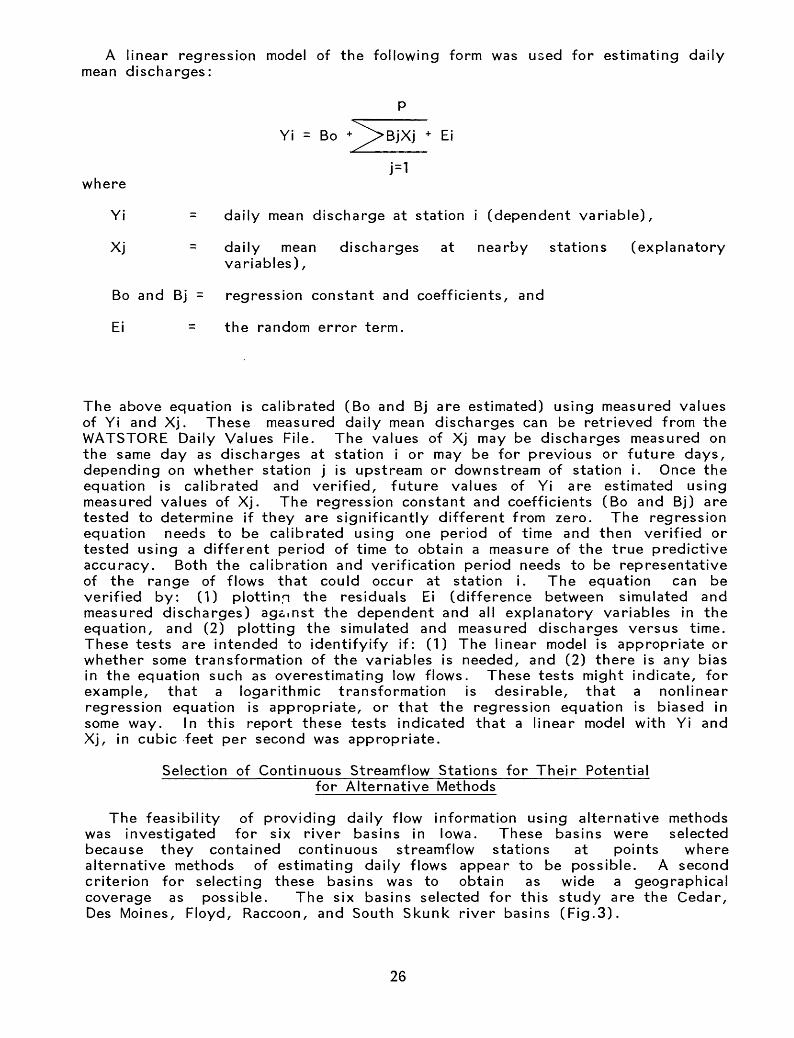
A linear regression model of the following form was used for estimating daily mean discharges:
Yi = Bo + BX + Ei
where
Yi = daily mean discharge at station i (dependent variable),
Xj = daily mean discharges at nearby stations (explanatory variables),
Bo and Bj = regression constant and coefficients, and
Ei = the random error term.
The above equation is calibrated (Bo and Bj are estimated) using measured values of Yi and Xj. These measured daily mean discharges can be retrieved from the WATSTORE Daily Values File. The values of Xj may be discharges measured on the same day as discharges at station i or may be for previous or future days, depending on whether station j is upstream or downstream of station i. Once the equation is calibrated and verified, future values of Yi are estimated using measured values of Xj. The regression constant and coefficients (Bo and Bj) are tested to determine if they are significantly different from zero. The regression equation needs to be calibrated using one period of time and then verified or tested using a different period of time to obtain a measure of the true predictive accuracy. Both the calibration and verification period needs to be representative of the range of flows that could occur at station i. The equation can be verified by: (1) plottinq the residuals Ei (difference between simulated and measured discharges) ag&.nst the dependent and all explanatory variables in the equation, and (2) plotting the simulated and measured discharges versus time. These tests are intended to identifyify if: (1) The linear model is appropriate or whether some transformation of the variables is needed, and (2) there is any bias in the equation such as overestimating low flows. These tests might indicate, for example, that a logarithmic transformation is desirable, that a nonlinear regression equation is appropriate, or that the regression equation is biased in some way. In this report these tests indicated that a linear model with Yi and Xj, in cubic feet per second was appropriate.
Selection of Continuous Streamflow Stations for Their Potentialfor Alternative Methods
The feasibility of providing daily flow information using alternative methods was investigated for six river basins in Iowa. These basins were selected because they contained continuous streamflow stations at points where alternative methods of estimating daily flows appear to be possible. A second criterion for selecting these basins was to obtain as wide a geographical coverage as possible. The six basins selected for this study are the Cedar, Des Moines, Floyd, Raccoon, and South Skunk river basins (Fig.3).
26

Fig
ure
3. S
tud
y a
reas
for
alte
rnat
ive
met
hods
of
pro
vid
ing s
trea
mfl
ow i
nfo
rmat
ion.
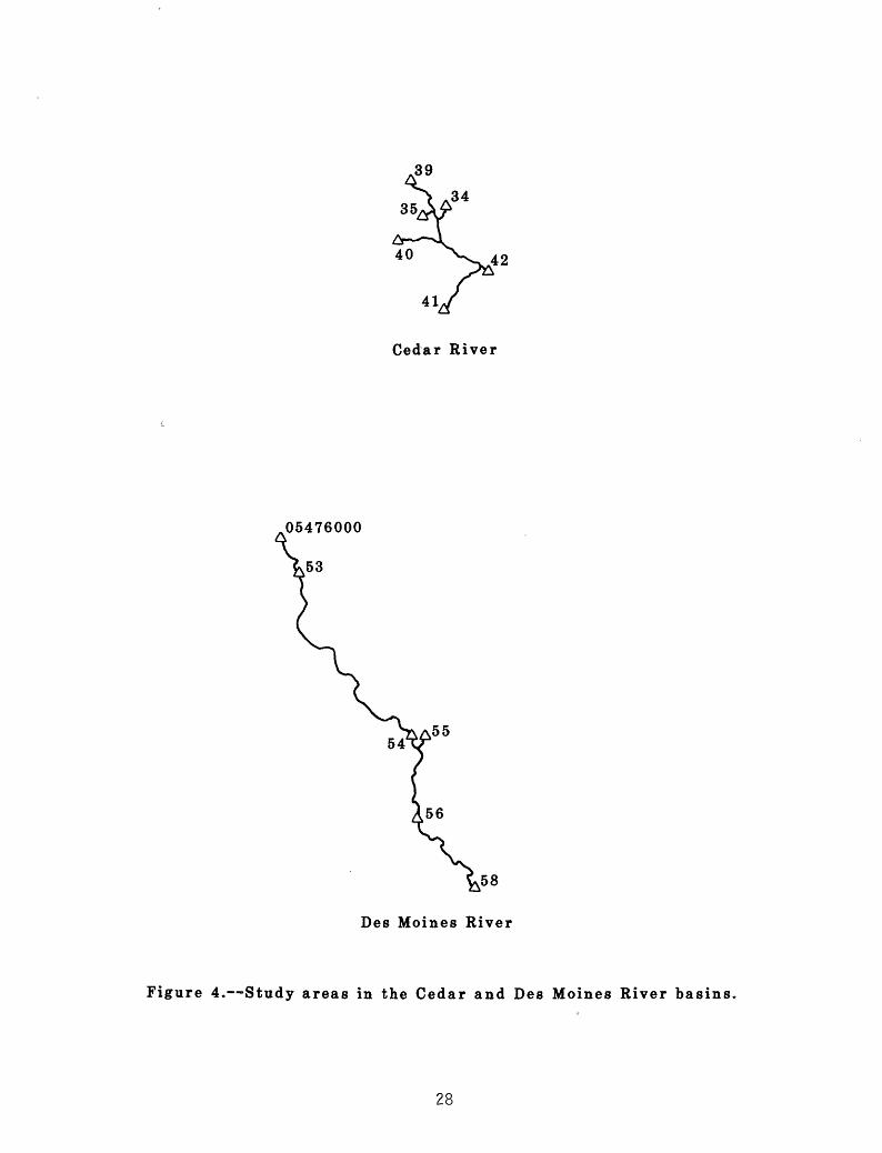
34
55
Des Moines River
Figure 4. Study areas in the Cedar and Des Moines River basins.
28

90
20
Iowa River
Figure 5. Study areas in the Floyd and Iowa River basins.
29

67
Raccoon River
,05471000
Skunk River
Figure 6. Study areas in the Raccoon and Skunk River basins.
30

Table 3. -- Selected characteristics used in the flow-routing studies
Station
34353940414647*
Basin
CedarCedarCedarCedarCedarS. SkunkS. SkunkDes Moines
Qoft /s
800462887189163147117
273
Wo ft
600450600150150132132
198
So ft/ft
0.000560.000680.000520.000800.000740.000690.00095
0.00053
dQ /dY ft /s
1050120175126107272284
271
Coft/s
1.750.270.290.840.762.062.15
3.67
Ko ft/s
1190755
1421788689807467132
* 5-4760 Gaging station in MinnesotaQo is the stream discharge in cubic feet per secondWo is the average channel width for the study reach in feetSo is the average bed slope in feet per feetYo is the average depth of flow in feetCo is the flood wave celerity in feet per secondKo is the wave dispersion or damping coefficient in feet squared per second
Table 4. -- Summary of flow-routing results and comparison between measuredand simulated flows
Station Basinnumber
4253
**
CedarDes MoinesS. Skunk
Period ofsimulation
(water years)
1980-811980-811978-79
Mean Percent of total simulated flowserror
(percent)
102010
within the indicated error5%
453035
10%
855065
25%
988593
>25%
215
7
** Station 5-4710 discontinued
31

Because of time and budget constraints, only a representative number ofstations was selected for this study. The District needs to continue to search,on a systematic basis, for stations where alternative methods could be applicable.
For the sake of brevity only the final results of model calibration and simulation are presented in this report. The details of estimating model parameters , techniques of model calibration and verification, methods for estimating intervening flows, and methods for selecting optimal estimators , have been documented and are available for reference at the District Office in Iowa City.
Both flow-routing and regression techniques were used to evaluate selected stations in the Cedar River (Fig. 4), Des Moines River (Fig. 5), and South Skunk River(Fig. 5) basins. Only regression techniques were used to evaluate selected stations in the Floyd River (Fig.6), Iowa River(Fig.4), and Raccoon River (Fig.6) basins.
The objective of the flow-routing analyses were to determine (1) If station 42 in the Cedar River Basin and station 53 in the Des Moines River basin could be discontinued, and (2) if a previous decision to discontinue station 05471000 in the South Skunk River basin was valid. Prior to its being discontinued in 1979 at the request of the cooperator, daily flows at station 05471000 were used by local authorities for a number of water management activities. It was assumed that daily flows of sufficient accuracy could be estimated by using the daily flows at stations 46 and 47. Aspects of the flow-routing analyses are summarized in tables 3 and 4. Selected reach characteristicsare summarized in table 3 and the results of the analyses are summarized in table 4. Regression models were developed for all the stations mentioned above, shown in figures 4-6, however, only the results for selected stations with the smallest errors in each of the basins are presented in table 5. The table includes the predictive equation for streamflow at each station and a comparison between measured and simulated streamflow.
The results of the analysis indicated that the simulated streamflows are not accurate enough to warrant using either alternative techniques in lieu of operating the gaging stations. However, it should be emphasized that these are preliminary results.
Based on these preliminary results:
1. It may be possible to use an alternative method for determining styreamflow in lieu of operating stations 42 in the Cedar River basin, but this possibility does not appear to exist for the other stations in the basin that were analyzed.
2. It appears that station 53 in the Des Moines River basin can not be discontinued, however, results of the regression analysis for station 56 in the same basin indicate that it may be possible to use an alternative method for determining streamflow in lieu of operating this station. All other stations in the basin that were analyzed need to be continued.
3. It appears that station 05471000 in the South Skunk River basin should not have been discontinued. Although the results obtained by using the flow-routing model appear to be slightly better (mean error 9.7 percent) than the results from the regression analysis (mean error 12 percent), neither are accurate enough to justify discontinuing the station.
33

Table
5.
Summ
ary
of re
gres
sion
-mod
elin
g results
and
comparison be
twee
n me
asur
ed and
simu
late
d da
ily
flows.
[ St
atio
n Ba
sin
Number
42 39 56 58 91 18 19 22 67GO 1X3
73
Cedar
Ceda
r
Des
Moin
es
Des
Moin
es
Floy
d
Iowa
Iowa
Iowa
Racc
oon
Racc
oon
5-47
10 Sk
unk
log(Q42)=
log(Q39)=
Q56
=
Q58
=
Q91
=
Q18
=
Q19
=
Q22
=
Q67
=
Q73
=
Q5-4
710
=
Predicti
ve Eq
uati
ons
Water years
used fo
r Ca
libr
atio
n Simulation
0.68 +
0.36
*log
(Q34
)+ 0.27* lo
g(Q3
5 )+
0.34*log(l_AG1 Q39)
0.11
4 + 0.70*log(Q34)+ 0. 30*
l og
(Q35
)
18.1 +
1 .14*Q54
176+1 .27
*Q56
150+1 .58
*Q89
7.04
+
0.49
*Q19
1.16+ 0.39*Q
21
7.11
+
0.76
*Q18
210
+ 1 .66(
l_AG
1
589
+ 1 .03(l_
AG1
5.51 +
1.16
*Q46
+ 1 ,24*Q55
+ 1.33 (LA
G! Q90)
+ 0.
43*Q
22
+ 0.
14*Q
22
+ 0.60*Q19 +
0.78*Q21
Q65)
Q67)
+
2.44
(LAG
1 Q71
)
+ 0.
98*Q
47
1976-79
1976-79
1976
-79
1976-79
1976
-79
1976
-79
1976
-79
1976
-79
1977-79
1977
-79
1973-77
1980-81
1980
-81
1980
-81
1980-8
1
1980
-81
1980-8
0
1980-8
0
1980
-80
1980
-81
1980
-81
1978-7
9
Mean
error
9 18 12 20 30 20 20 13 25
28 12
Perc
ent
within
53 30 40 32 14 26 18 20 20
20 40
of to
tal
simu
late
d flows
the
indicated
erro
rs
10%
25%
>25%
77 51 72 51 30 53 40 42 40
39 65
96 84 93 80 70 82 80 80 84
75 90
4 16 7
20 30 18 20 20 16
25 10
LAG1
is
a
variab
le cr
eate
d by la
ggin
g th
e di
scha
rges
at an in
depe
nden
t station
by
1 da
y. This ac
coun
ts for
the
travel ti
me be
twee
n th
e two
stations
.

4. No stations in the Floyd River, Iowa River, and Raccoon River basins can be discontinued at this time. It may be possible to decrease the errors in the preliminary results by 50 percent, but even then it is likely that the estimated flows would not meet the accuracy requirements.
Summary of the Second Phase of the Analysis
In general the data simulated by using the flow-routing and regression methods for the stations included in this study did not meet the accuracy needed to consider these methods as alternatives to operating gaging stations. However, as a result of this study, the three gaging stations with significant potential as alternative method sites that have been identified are:
1. Cedar River at Waterloo (station 42).
2. Des Moines River at Fort Dodge (station 56).
3. South Skunk River below Squaw Creek near Ames (station 05471000, discontinued).
The District should study these sites in more detail. Final decisions regarding these gaging stations will be made after the results of the additional studies have been evaluated and discussed with the appropriate cooperating agencies.
If an acceptable alternative method can not be developed for the site of the former gaging station in the South Skunk River basin, then the District needs to take the necessary steps to reactivate the gaging station or to establish a new station downstream from the point of discharge of effluent from the waste treatment plant at Ames.
The District also needs to continue with the identification of gaging stations in other basins where alternative methods could be used. In summary, all the stations considered in this step of the analysis need to be continued and were included in the third and final phase of the analysis.
COST-EFFECTIVE RESOURCE ALLOCATION
Introduction to Kalman-Filtering for Cost-Effective Resource Allocation (K-CERA)
A set of techniques called K-CERA were developed by Moss and Gilroy (1980) to study the cost-effectiveness of networks of stream gages. The original application of the technique was to analyze a network of stream gages operated to determine water consumption in the Lower Colorado River Basin (Moss and Gilroy, 1980). Because of the water balance nature of that study, the minimization of the total variance of errors of estimation of annual mean discharges was chosen as the measure of effectiveness of the network. This total variance is defined as the sum of the variances of errors of mean annual discharge at each site in the network. This measure of effectiveness tends to concentrate stream-gaging resources on the large rivers and streams where discharge and, consequently, potential errors are greatest. Although this may be acceptable for a water- balance network, considering the many uses of data collected by the U. S. Geological Survey, concentration of effort on large rivers and streams is undesirable and inappropriate.
34

MG Minimize V = T. (j). (M.)
7=1 ^ ^
F = total uncertainty in the network
N_ = vector of annual number times each route was used
MG = number of gages in the network
M . =. annual number of visits to station jJ
cj) . E function relating number of visits to uncertainty at station j
Such that
Budget _> T Etotal cost of operating the networkc?MG NR
T = F + Za.M. + Z 3 .fl .0 ° '1''1
F = fixed cost o
a. = unit cost of visit to station jJ NR = number of practical routes chosen
3. = travel cost for route i^N. =. annual number times route i, is used i
(an element of N)
and such that
M. > A. J - J
A. ^ minimum number of annual visits to station3
Figure 7. Mathematical programing form of the optimization of the routing of hydrographers.
35

Route
12
3
4
z
.
NR
UnitVisit CostMinimum VisitsVisits
Uncert.Pi inr'tinn
Gage 1 2 3 4 . j . MG
1 0 0 0 ... 0
1 1 0 0 ... 0
1 0 0 0 ... 0
0 1 0 0 ... 0
..... CO j ' . .
. .....
. .....
0 0 0 0 ... 1
a, a2 «3 a4 . a. . aMG
*/ \/ 1 */ 1/ 2 *^ ^3 4 * 7 * ft^^^
M, M2 M3 M4 . ^ . MMG
01 02 03 04 ' 0/ ' 0MG
Unit Travel Cost
faP>2
f$3
04
0,'
.
0NR
vAt-sit( Cost
^* ^
N
Uses
N,N2
N3
N4
N;
.
Nm
t ^ ^ Travel
Cost** /
k rrTotal _ /:cost v:
Total Uncertainty
Figure 8. Tabular form of the optimization of the routing of hydrographers.
36

The original version of K-CERA was therefore altered to include as optional measures of effectiveness the sums of the variances of errors of estimation of the following streamflow variables; annual mean discharge, in cubic feet per second; annual mean discharge, in percent; average instantaneous discharge, in cubic feet per second; or average instantaneous discharge, in percent (Fontaine and others, 1983). The use of percentage errors effectively gives equal weight to large and small streams. In addition, instantaneous discharge is the basic variable from which all other streamflow data are derived. For these reasons, this study used the K-CERA techniques with the sums of the variances of the percentage errors of the instantaneous discharges at continuously gaged sites as the measure of the effectiveness of the data-collection activity.
The original version of K-CERA also did not account for error contributed by missing stage or other correlative data that are used to compute streamflow data. The probabilities of missing correlative data increase as the period between service visits to a stream gage increases. A procedure for dealing with the missing record has been developed (Fontaine and others, 1983) and was incorporated into this study.
Brief descriptions of the mathematical program used to minimize the total error variance of the data-collection activity for given budgets and of the application of Kalman filtering (Gelb, 1974) to the determination of the accuracy of a stream- gaging record are presented by Fontaine and others (1983). For more detail on either the theory or the applications of the K-CERA model, see Moss and Gilroy (1980) and Gilroy and Moss (1981).
Description of Mathematical Program
The program, called "The Traveling Hydrographer," attempts to allocate among stream gages a predefined budget for the collection of streamflow data in such a manner that the field operation is the most cost-effective possible. The measure of effectiveness is discussed above. The set of decisions available to the manager is the frequency of use (number of times per period) of each of a number of routes that may be used to service the stream gages and to make discharge measurements. The range of options within the program is from zero use to daily use for each route. A route is defined as a set of one or more stream gages and the least cost travel that takes the hydrographer from his base of operations to each of the gages and back to base. A route will have associated with it an average cost of travel and average cost of servicing each stream gage visited along the way. The first step in this part of the analysis is to define the set of practical routes. This set of routes usually will contain the route to an individual stream gage with that gage as the lone stop and return to the home base so that the individual needs of a stream gage can be considered in isolation from the other gages.
Another step in this part of the analysis is the determination of any special requirements for visits to each of the gages for such things as necessary periodic maintenance, rejuvenation of recording equipment, or required periodic sampling of water-quality data. The minimum number of visits to each gage usually are limited by these special requirements.
The final step is to use all of the above to determine the number of times that each route is used during a year such that: (1) The budget for the network is not exceeded, (2) the minimum number of visits to each station is made, and (3) the total uncertainty in the network is minimized. This step in the form of a mathematical program is presented in figure 7. A tabular presentation of the problem is presented in figure 8. Each of the routes is represented by a row of
37'

the table and each of the stations is represented by a column. The zero-one matrix defines the routes in terms of the stations that comprise it. A value of 1 in the row indicates that gaging a station will be visited on the route; a value of zero indicates that it will not. The unit travel costs are the pen-trip costs of the hydrographer's traveltime and any related per diem and operation, maintenance, and rental costs of vehicles. The sum of the products of the unit travel costs multiplied by the times the route was used is the total travel cost.
The unit-visit cost is comprised of the average service and maintenance costs incurred on a visit to the station plus the average cost of making a discharge measurement. The minimum visit constraints are set for each station. The product of the visits to each station per route and the times the route is used must equal or exceed the minimum visit constraints.
The total cost expended at the stations is equal to the sum of the products of unit cost and number of visits for all stations. The cost of record computation, documentation, and publication is assumed to be affected negligibly by the number of visits to the station and is included in the fixed cost of operating the network. The total cost of operating the network equals the sum of the travel costs, the at-site costs, the fixed cost, and the overhead cost, and needs to be less than or equal to the available budget.
The total uncertainty in the estimates of discharges at all the stations in the network is determined by summing the uncertainty functions evaluated for the total visits to all stations.
As pointed out in Moss and Gilroy (1980), the steepest descent search used to solve this mathematical program does not guarantee a true optimum solution. However, the locally optimum set of values obtained with this technique specify an efficient strategy for operating the network, which may be the true optimum strategy. The true optimum strategy cannot be guaranteed without testing all undominated, feasible strategies.
A detailed description of the uncertainity function (Fontaine and others, 1983) and a similar description of for the method for deriving the relationship of visit frequency to lost record (Moss, 1983), as published in the report of the pilot study of cost effectiveness in Maine, are found in the Supplemental Data section of this report.
It is assumed in this study that the differences between the logarithms of the computed discharges and the true discharges at each instance are normally (Gaussian) distributed with a mean of zero and a variance of either Vf, Vr, or Ve depending on whether the at-site streamflow recorder was functioning (f), whether the record was reconstructed (r) from another primary source of data, or whether the record was estimated (e) without the aid of other concurrent data. Therefore, the resulting apriori distribution of errors is not normally distributed in terms of the logarithms of discharge data. This lack of normality causes difficulty in interpretation of the resulting errors of estimation, that is, the square root of the uncertainty contained in the streamflow record. If the logarithmic errors were normally distributed, approximately two-thirds of the time the true logarithmic error would be within the range defined by plus and minus one standard error from the mean. The lack of normality caused by the multiple sources of error increases the percentage of errors contained within this range to more than above that of a Gaussian probability distribution of logarithmic errors with the same standard deviation.
38

To assist in interpreting the results of the analyses, a new parameter, equivalent Gaussian spread (EGS), is introduced. The parameter EGS specifies the range in terms of equal positive and negative logarithmic units from the mean that would encompass errors with the same apriori probability as would a Gaussian distribution with a standard deviation equal to EGS; in other words, the range from -1 EGS to + 1 EGS contains about two-thirds of the errors. For Gaussian distributions of logarithmic errors, EGS and standard error are equivalent. EGS is reported herein in units of percentage and an approximate interpretation of EGS is, "Two-thirds of the errors in instantaneous streamflow data will be within plus or minus EGS percent of the reported value."
The Application of K-CERA in Iowa
A rating analysis to define the time series of residuals was performed on 100 of the 110 continuous streamflow stations in Iowa. Discharge measurements were considered for the past 10 years. The residuals of measured discharges from the long-term rating were analyzed by time series technique to determine the input parameters of the Kalman-filter streamflow records. The error variance, Vf, was computed as a function of the time-series parameters, the discharge-measurement- error variance and the frequency of discharge measurement. The rating function for all stations was of the form:
LQM = B1 + B3 * LOG(GHT - B2)
where
LQM is the logarithm (base e) of the measured discharge;
GHT is the record gage height of the measurement, in feet;
B1 is the logarithm of discharge for a flow depth of 1 foot;
B2 is the gage height of zero flow, in feet; and
B3 is the slope of the rating curve.
The various functions for each station are listed in table 6. The rating analysis was based on open-water conditions only. Backwater from ice can be expected on an average of 3 months per year and seriously affects the stage- discharge relation. In general, stage-discharge ratings for the Iowa stations are subjected to shifting control, especially in the low-water range because of scour and fill of alluvial material.
From the residuals of the rating analysis, the 1-day auto-correlation coefficient, process variance, and discharge-measurement variance were computed. Four other stations had been analyzed in a previous study (Kitanidis and others, 1984) of the Missouri River ratings. These data were added to the study at this point. Six stations were not included in this study and were processed as stations with zero weight in the traveling hydrographer program. They were the following: (1) Mississippi River at McGregor (05389500), Mississippi River at Clinton (05420500), and Mississippi River at Keokuk (05474500) that require slope ratings and were not analyzed by Kalman-filtering techniques; and (2) Crow Creek at Bettendorf (05422470), Middle Raccoon River near Newell (05482135) and Perry Creek at Sioux City (06600000) that had too short a period of record for a rating analysis.
39
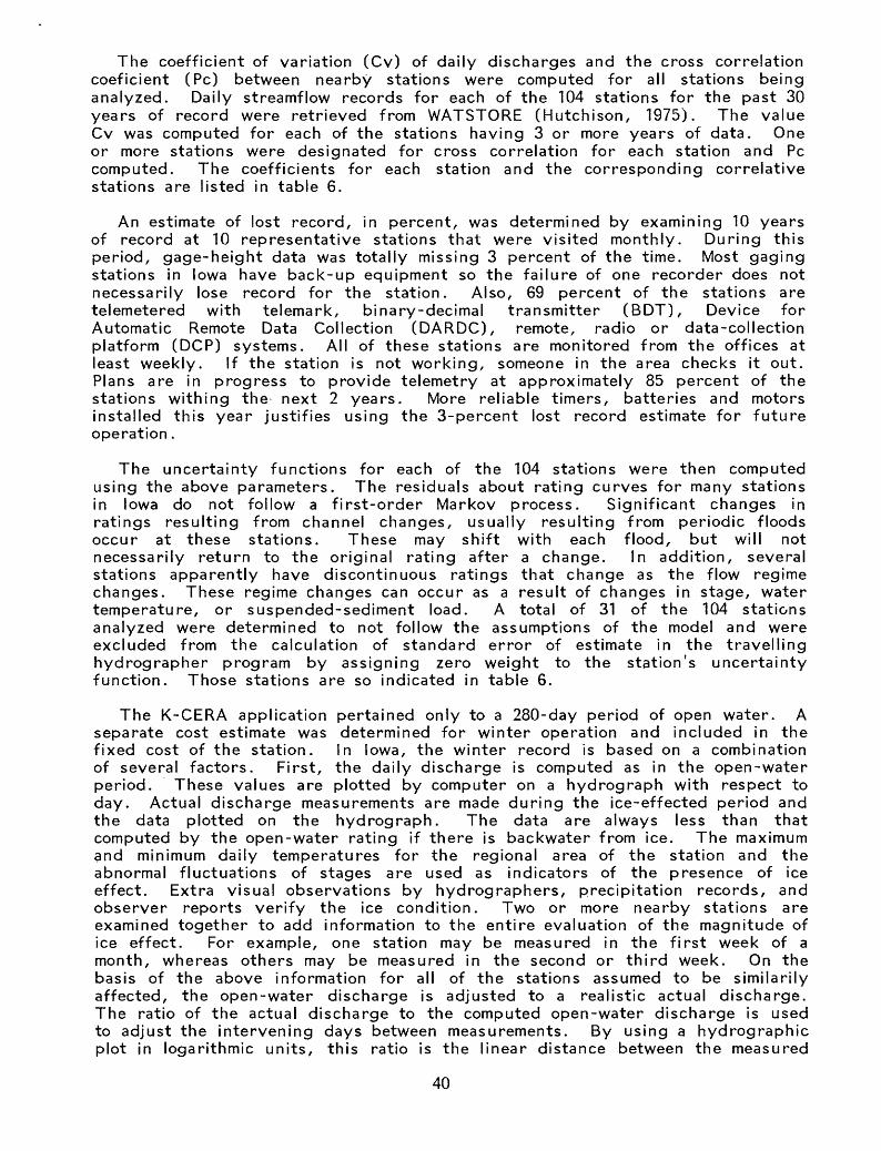
The coefficient of variation (Cv) of daily discharges and the cross correlation coeficient (Pc) between nearby stations were computed for all stations being analyzed. Daily streamflow records for each of the 104 stations for the past 30 years of record were retrieved from WATSTORE (Hutchison, 1975). The value Cv was computed for each of the stations having 3 or more years of data. One or more stations were designated for cross correlation for each station and PC computed. The coefficients for each station and the corresponding correlative stations are listed in table 6.
An estimate of lost record, in percent, was determined by examining 10 years of record at 10 representative stations that were visited monthly. During this period, gage-height data was totally missing 3 percent of the time. Most gaging stations in Iowa have back-up equipment so the failure of one recorder does not necessarily lose record for the station. Also, 69 percent of the stations are telemetered with telemark, binary-decimal transmitter (BDT), Device for Automatic Remote Data Collection (DARDC), remote, radio or data-collection platform (DCP) systems. All of these stations are monitored from the offices at least weekly. If the station is not working, someone in the area checks it out. Plans are in progress to provide telemetry at approximately 85 percent of the stations withing the next 2 years. More reliable timers, batteries and motors installed this year justifies using the 3-percent lost record estimate for future operation.
The uncertainty functions for each of the 104 stations were then computed using the above parameters. The residuals about rating curves for many stations in Iowa do not follow a first-order Markov process. Significant changes in ratings resulting from channel changes, usually resulting from periodic floods occur at these stations. These may shift with each flood, but will not necessarily return to the original rating after a change. In addition, several stations apparently have discontinuous ratings that change as the flow regime changes. These regime changes can occur as a result of changes in stage, water temperature, or suspended-sediment load. A total of 31 of the 104 stations analyzed were determined to not follow the assumptions of the model and were excluded from the calculation of standard error of estimate in the travelling hydrographer program by assigning zero weight to the station's uncertainty function. Those stations are so indicated in table 6.
The K-CERA application pertained only to a 280-day period of open water. A separate cost estimate was determined for winter operation and included in the fixed cost of the station. In Iowa, the winter record is based on a combination of several factors. First, the daily discharge is computed as in the open-water period. These values are plotted by computer on a hydrograph with respect to day. Actual discharge measurements are made during the ice-effected period and the data plotted on the hydrograph. The data are always less than that computed by the open-water rating if there is backwater from ice. The maximum and minimum daily temperatures for the regional area of the station and the abnormal fluctuations of stages are used as indicators of the presence of ice effect. Extra visual observations by hydrographers, precipitation records, and observer reports verify the ice condition. Two or more nearby stations are examined together to add information to the entire evaluation of the magnitude of ice effect. For example, one station may be measured in the first week of a month, whereas others may be measured in the second or third week. On the basis of the above information for all of the stations assumed to be similarily affected, the open-water discharge is adjusted to a realistic actual discharge. The ratio of the actual discharge to the computed open-water discharge is used to adjust the intervening days between measurements. By using a hydrographic plot in logarithmic units, this ratio is the linear distance between the measured
40

and computed values. This distance can be varied between measurement dates or control points by considering the trend in temperatures and abnormal gage-height flucuations.
Winter records with severe backwater from ice at stations in Iowa are rated poor (>15 percent). The magnitude of ice effect may vary during the day. An actual discharge measurement every day would improve the accuracy of the record but the data may still be in considerable error. The ice effect usually is more consistent if the stream surface freezes completely at the beginning of winter and remains frozen until spring. A discharge measurement made soon after the freeze, one during the middle of winter and one just before melting, can give a fairly good trend for the whole period. However, this situation seldom happens as temperatures fluctuate enough to cause cyclic periods of ice cover and open water. For this study, three ice measurements per year were budgeted at twice the open-water unit and route costs and entered in the fixed cost of the station.
Visit costs are those associated with paying the hydrographer for the time actually spent at a station servicing the equipment and making a discharge measurement. These costs vary from station to station and are a function of the difficulty and time required to make the discharge-measurement Average visit times were calculated for each station based on an analysis of discharge- measurement data available. This time was then multiplied by the average hourly salary of hydrographers in the Iowa offices to determine total visit costs. Route costs include the vehicle cost associated with driving the number of miles it takes to cover the route, the cost of the hydrographer's time while in transit, and any per diem associated with the time it takes to complete the trip.
K-CERA Results
The "Traveling Hydrographer Program" uses the uncertainty functions along with the appropriate cost data and route definitions to compute the most cost- effective way of operating the stream-gaging program. In this application, the first step was to simulate the current practice and determine the total uncertainty associated with it. To accomplish this, the number of visits being made to each stream gage and the specific routes that are being used to make these visits were fixed. In Iowa, current practice indicates that discharge measurements are made 90 percent of the time that a station is visited. The resulting average error of estimation for the current practice in Iowa is plotted as a point in figure 9 and is 11.4 percent.
The upper line in figure 9 represents the minimum level of average uncertainty that can be obtained for a given budget with 3 percent lost record and the existing instrumentation and technology. The line was defined by compiling results of several runs of the traveling hydrographer program with different budgets for each of the three offices. Constraints on the operations other than budget were defined as described below. The lower line defines the average uncertainty versus budget considering no lost record.
Except for the 3 index stations, 5 Missouri and 3 Mississippi River stations, streamflow stations are currently visited every 6 weeks in Iowa. Consideration is given to the physical limitations of the equipment at the gage, such as battery duration, capacity of the tape spools of the recorder, purging of the orifice line or intakes, nitrogen-gas supply, and freezing problems. The effect of visitation frequency on the accuracy of the data and the quantity of lost record is taken into account in the uncertainty analysis. In Iowa, a minimum requirement of 5 visits during the open water season (280 days) was designated; for the winterseason, the minimum was 3 visits.
41
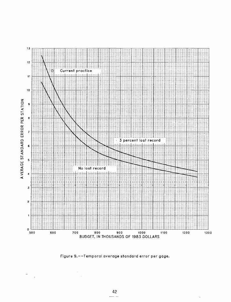
500 600 700 800 900 1000 1100
BUDGET, IN THOUSANDS OF 1983 DOLLARS1200 1300
Figure 9.--Temporal average standard error per gage.
42

Table
6
.
Sum
mar
y o
f th
e
Ka
Ima
n-f
iIte
rin
g
an
aly
sis
.
Stationl
no.
ISt
atio
n name
iRating
coefficients
|I
81
| 82
|
B3
| RH
OVPROC
Unce
rtai
nty
| |
iCor
rela
ted
2 |
5 I
10
I 20
I
Cv
| PC
|
sta.
no.
CO
[81,
B2,
and
B3 =
coefficients as shown
for
the
rating fu
ncti
on LQM
= B1 +
B3 *
LOG(
GHT
- B2);
RHO
= 1-
day
autoco
rrelation
coef
fici
ent;
VP
ROC
= process
vari
ance
(l
og base e);
Unce
rtai
nty
= un
cert
aint
y fu
ncti
on,
in
percent
error, with respect
to nu
mber
of measurements pe
r pe
riod
(2
80 day);
Cv =
coefficient
of variation
of
dail
y values;
PC =
cross
correlation
of da
ily
stre
amfl
ow va
lues
wi
th ne
arby
st
atio
n as li
sted
(l
og ba
se 10)]
Uppe
r Iowa River
Basin
0538
7500
Upper
Iowa R
at De
cora
h | 5.
34
| 3.08
I 1.92 |0
.996
70 |0
.036
92 |17.0| 9.
2| 6.1| 4.211.37610.97
I 05
4116
00
0538
8250
Upper
Iowa
R
nr Do
rche
ster!
5.13
I 6.
05
I 1.82
| .96526
I .00694 |10.8| 7.4| 5.5I 4.0|
.728
! .98
I 05
3875
00
Turkey River
Basin
0541
1600
Turkey R
at SpillvMIe
0541
2500
Turkey R
at Garber
Maquoketa
River
Basin
0541
8450
NF
Maquoketa
R at
Fu
lton
05
4185
00 Ma
quok
eta
R nr Maquoketa
Waps
ipin
icon
Ri
ver
Basin
0542
0560
Wapsipinicon R
nr El
ma
0542
1000
Wa
psip
inic
on R
at Indepndnl
0542
2000
Wapsipinicon R
nr DeWitt
Iowa
R
i ve r
Ba s i n
0544
9000
EB Io
wa R
nr Klemme
0544
9500
Io
wa R
nr Rowan
0545
1500
Iowa R
at Marshal
I town
0545
1700
Ti
mber
C
nr Ma
rsha
lIto
wn
0545
1900
Richland C
nr Haven
0545
2000
Salt C
nr Elberon
0545
2200
Walnut C
nr Ha
rtwi
ck
05453000 Bi
g Bear C
at Ladora
0545
3100
Io
wa Ri
ver
at Ma
reng
o 05
4540
00 Rapid
C nr Io
wa City
0545
4300
Cl
ear
C nr Cora I vi
Me
0545
4500
Io
wa R
at Io
wa City
05455000 Ra
lsto
n C
at Io
wa Ci
ty
0545
5010
SB Ra
lsto
n C
at Io
wa City
0545
5500
En
glis
h R
at Kalona
1 .49
5.35
I 4.
74
5.08
I 2.81
I 6.
16
I 3.
16
4.00
3.
94
2.11
3.
28
2.04
2.74
2.98
3.18
4.36
1.52
3.61
5.68
0.38
1.62
4.07
1 .70
I 4.
83
I 2.
27
I 8.90
3.13
I 4.
33
1 .22
2.34
2.61
4.50
1 .22
8.58
3.81
2.86
9.50
3.15
2.39
1 .80
8.59
1.52
1.
15
1.64
I 3.
00
I 1.
53
I 1.
72
1.58
1.83
1.
57
2.50
1.53
1.70
2.85
1 .8
0 3.
07
2.00
2.08
2.01
1 .8
4 2.99
1.78
1 .42
4.95
3.04
1 .8
1
.97899
I .99232
I .98386
.97270
.98000
.95646
.97642
.97899
.98076
.99055
.97270
.98076
.96651
.98798
.98557
.97975
.97899
.97848
.94382
.97899
.96554
.98284
.060
47 124.7117.1112.41 8.8|1.353|
.97
.015
23 11
6.81
9.
61 6.51 4.5H. 248
1 .95
.003
46
I 8.21 4.81 3.
31 2.
31 .6
601
.87
.00693 11
3.71
8.
1| 5.7| 4.0|1.141| .9
8
.016
15 123.2113.81 9.51 6.6|1.722| .92
.014
85
121 .0113.7110.1 I
7.311.4881 .9
5 .0
2925
11
9.71
13.4
1 9.8| 6.9M.147I .9
4
.028
26 125.1 11
5. 4110.71 7.5M.831I
.96
.011
27 119.1110.61 7.11 4.811.6571 .9
8 .1
018
126.2116.6111.61 8.1|1.377|
.93
.021
26 12
0.41
12.5
1 8.8| 6.211.6961 .9
9 .1
486
I 2
\ 2
I 2
I 2
11.8421
.98
.038
49 126.0117.7113.11 9.
4 |1.
697
I .9
6 .1
871
I 2
\ 2
I 2
\ 2
11.9
041
.99
.058
44 |25. 011
5. 2|10.4| 7.2|1.835I .9
9 .0
3268
118.8112.61 9.0| 6.4|1.183| .9
8 .1
198
I 2
I 2
I 2
I 2
12.0611
.99
.166
9 \
2 \
2 \
2 \
2 11.8241
.98
.003
65 11
1.81
6.91 5.0| 3.711.0781 .99
.107
5 \
2 \
2 \
2 \
2 12.1521
.99
.213
8 \
2 \
2 \
2 \
2 11.8511
.99
.112
5 13
2.81
21 .7115.3110.711 .95
21 .9
8
05388250
1 05411600
I 05412500
05418450
05412500
05422000
05421000
05459500
05449000
05449500
05451900
05452000
05453000
05451900
05452200
05451500
05454300
05455500
05455700
05455500
05455000
05453000
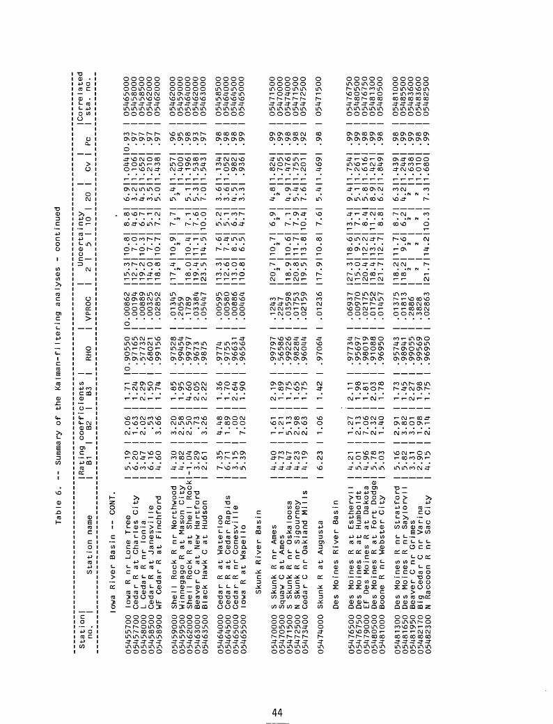
1717
oooooVJl VJl VJl VJl VJl
00 00 00 00 00ro ro -> -» ->Co i NO ON CoO -JVJlVJtOoooooZ 03 03 CJ O CO CD CO
T;IQ 03 co co03 <0 OCO 22 O CO -5 O O O Q. O 03 O 3 3 3-5 CD CO
3 cn co33 O -5
33 73 3 3 O -5-5-533
CO < 3 "* "*
03 03 CD CO COO -5 cn Q3 rt- << -5
O 3 03 03 O rt Ct -5 -»3<< < 0
Q.
4=- ro oo vjt vji »NQ Co 00 VJ1O -> rOON
ro -» co co ro->NO O 00 NO-FOO - ro -»
->|NO ro 4="->l VJl 00 ->l VJl 00
VO NO NO NO NOON NO NO 00 VJl NO VJl ONQ -vjVJl ON VJl jr-F O VO VJl » Co
OCo rOOOro oo oo -» -» oo ro co oo coON 00 ON ' J Co Co VJl
-> 0000
->l ro ro
4T NQ->
M ON->I
O ONOO
co ro ^j
-J -FON
co roco
ONOONrO -F 00 -i Co .F oo O O 00 4=- NO
NO NO NO NO NO NO 00 NO NO 00
oooooVJl VJl VJl VJl VJl
00 00 00 CO 00ro oo oo vji -»VJl ON ON VJl Oooooo ooooo
oooooVJl VJl VJl VJl VJl
00 00 -J ->I-J -1 ONO ON ONovjto->ivjiO O OVJi Oooooo OBomooO CO TI CO CD O cn co co 3 O CD 2CD 22
O cn O O TJ _. _. _.
3233 3 CO O CO CD -5 cn co cn
3 SI 33 CD 73 73 co cnOf 03 03 03 Cn ct 73 rt ct rtCD TI 03 x m -5 O ct c cn
-5 3 ct O ct O OT3- 03 O CO ct OX -5 << O O Q.<
O.ct ct IQ 03 CO
VJl VJl -PVJI -F
O->INOO ro 00 00 ON -» -»
-> ro-J ro -»4Tcoo -> ro o ro ON co -vj
->l O 00 NO -> 00 Co i 00 »
NO NO NO NO NO ON -*COVJI ^J NO OOON->I VJl 00 > NO CO O 00 NO -J4=-
ooooo -> -> roooN4=- ->| -» NO NO VJl VJl ~J -J CO-j rovjio->i
-» 00 OVJI ^J
-jjrjroco
roco ro NO oo
->l jr ro vji ON_i _i
00 » 00 ->l CO
oo ro^ ->-F
ON 00 VJl VJl NO
roNO oo -j -F
oo jr ON ro ^J -F ro -» ONVJINO ->ON-> JT
NO NO NO NO NO 00 NO 00 NO VO
oooooVJl VJl VJl VJl VJl
00 00 ^J 00 -~J O -J ONOON VJl CO ^J VJl ->l O OVJI OVJIooooo
oCO cn
2o3 CO cn
73
<CD-5
03 0) CO
3
05474000 Skunk R at Augusta
ON
ro00
_.
0ON
""*
-p ro
NO-^i0ON.{=
o roCOON
->l
NO
0
00
->l
ON
VJl
-F
*
-F ONNO
NO00
05471500
oooooVJl VJl VJl VJl VJl
co ro -> oo-FVJl VJIVJIOooooo oooooO2 CO CO CO CD .Q Q. CO CO C CO03 X X03 X -5 C C < C
33 3 O X X O X
3 73 73 03 73 -5 Ct
33 3 O -5 -5 > -503 3xco o co > co co 3031Q X CD 3 O 03 cn Q-C
-5 0230 CD cn << 03
V)
*««
-i ro -F->l jrNO CO ^J CO O
ro rovji - ->ON NO ' ro ON Co 00 Co -i ->
->ION->I 00 -» VJl VJl VJl NO NO
NO NO NO VJl NO ON 00 NO ON NOo ro ro vji ^J 4=- oo ro oo vo£r 4=- ON ON ^J
oo o ro - ro ->co ro roVJl VJl NO ->l Co NO Co 00
NO O 00 O
VJl 00 NO ^J
Co -. o O
CO-J ON ->l
O->l -J ON
4=-NO -* NO
->IVJi jr -F
ON jrvo 00
ro ^j 4^ ^J oo ovji ^J o ro-*VJI ON VJl 4T
NO NO NO NO NOro oo oo NO NO
oooooVJl VJl VJl VJl VJl
ro _» 4r o -»VJl VJl O OVJIooooo ooooo
Skunk River Basin
ooooVJl VJl VJl VJl
ON ON ON ONVJl VJi 4=--F VJIOVJI Ooooo oooo ooo O CD CD CD < Q.Q.Q. 03 Q3 03 03
-5-5-5
73 737373
03 Ct D 03 03
-5 Ct ct
03 OO^ T3 O CD 03 CD 3 act CD 03 CO cn -5 -5 0 < - 73 0 03 O T3 CD
Q.cn
VJl CO ON ->l
Co -J ^J co NO VJl -» VJl
->l -'-F
0000-FrooNo oo
NO ON -^J COO4=- OON
NO NO NO NOON ON ^J ->lVJl ON VJl ->l ON Co VJi 4=- 4=- -»
OOOO OOOO4T CO VJI VJI ON 00 00 NO 4TONOVJI
oco ro co
00 O ON Co
ONOO ^J ->l
VJi VJi -fr ON
-F ON VJl VJl
->|CO _l fNJ
Co 4T Co Co
CO VJI ON ON
NONOO -> Co 00 VJI CoONror\>4=-
NO NO NO VO NO 00 00 00
ooooVJl VJI VJI VJI
ON ON ON VJIVJi 4^ 4=- 00 OVJIO VJIoooo oooo
oooooVJI VJI VJI VJI VJI
ON ON ON VJI VJIco co ro NO NOVJIOOVJIOooooo ooooo03 03 COS! CO CD 3- 3" 03 03 CD 3 CD 0 < -3 - XCD <D
-5 10 X 73 03 73 03 O OIQ O < 000 XOi X X
ct 73 O 73 73
Z 03 03 CD 03 ct D Ct < ct -5
X X CO 03 2 C 03 ITCn O DL -5 CD O -5 W ct D ct O -i> 3- 3 0 O<
-5 73 O QtO ct O
0<< Q. X
(NOW _> 4T4T
ON ro o oo co -> NO 4=- roo
oo ro ro oo
ro ->i vji vji roONOJ O OOO
roooNNooo ro vji ovji vji
VO NO NO NO NO CO ON NO NO ^J
vji OJNOVJI ro ^14^00
oo -» roo VJl OJ ^J O -» f CO 00 VJl CO 4=- CO NO NO -F->|.F NJI
ro-- -> -*oo NO 00 ->l
Vji4^O 4^
-F->0 0
VJi-> 4r NO
O ^J ^J ^J
OON-- -J
-vj VJI VJI VJI
Ooo -> -F
VJi VJi -» fr ro 4^0J NO OVJI Co 00 ONO ^J
NO NO NO NO NO -J OO 00 VJI ON
oooooVJI VJI VJI VJl VJI
ON ON ON VJI ONoo ro 4=- NO ro ooooo ooooo ooooo
oooooVJI VJI VJI VJI VJI
VJl VJI VJI VJI VJI 00 00 00 ^J VJI NO VJIO ^J ^Jooooo ooooos:or o- o -n co co o <
Q. O Q-< 03 O 03 CD 03 03 CO -5 Q. -5 73 0. 03 73 03 73 -5 73 < -5 3 CD
03 73 03 -5 -i 73ct rt
3 r 03 03 C_ -5 O O 0) Ct 03 3-D Cn
3 _ 03 CO T| CD O -5 3 cn 3 13 < CD -5 1O 03 cn CO I 3- CD ->) O O 0 CO O -5 rt Z 0- << H
4T ON CO ON VJI
ON -> 4^ ro -»OON->IONO
co ro -> roONVJIO ONOON oo ro co ON
-j vji ro ro -J F ONO-F -»
oNO ON VJi NO NONO 00 ^J ^J O _i O ^J -» VJlvji roco ON vji ON -> rovji o
oooooo ro oooo00 Co 00 - 00vji ro oo NO ON rovjiNQ4=-ro
oo fr NO ro vji
oo o ro-joo
0->IO-JO
->l ->l oo O 00
->| VJl ON 4=- 00
ro _i ^JONOO *
VJl Co 4^ oo ON
ovji vji ro NO
-Fro ON -*oCo -* VJI O foo o ro ON 4^
oNO NO NO NO NO
oooooVJI VJI VJl VJI VJI
ON ON VJI VJI ONro ro oo oovjiO OVJI O Oooooo ooooo
Station I
no. | Station name
73 03
_ 1 .3 IQ
OO
ro -»s -b 0
CO ct CO
73Xo
<-o73 Oo
c.0CO
Ul-5ct
-» 3Oct
<<
ro0
o<
o
Corre lated sta. no.
HQ3or
CD
ON
1
C 3 3
Q
O -b
3"
XSO
303
1- }
rt CO
U3
033 03
<<
CO
'
003
3
CD

917
oooON ON ONON ON ON OOO OOO Ul CO » OOO OOO
03 o o << Tl^O. O.
O 73<< 73
a.QJ Q)
ct 33 ct
C-3 >QJ -5 __
3 ct CD Crt OCO ct 3
T
CT
co ro coON.p->l
O ON P CO ON Oo o
CO-n co oo c
OON.pCO(A)
Ulo o
oCO O co ?roC 73
OO OOOOO OOOOO OOOOO
NO CO ONO
CO CO CO 00 CO NO CO ->J ->ION
0000
o oCD CD co co
Q.
03 03 Oco c X3
o
00
O 33C CD CDX co co
CO Q> Ct Ct
03 CD ct 3 Q) O ct
CD CO CO C V5 << QJ 3 ct 3 C < CD .Q QJ 3 C
CD
CO CO CO CO CO ONUIUI.P.P O ONUl COVJio^-o oo ooooo
CO CO CO CO CO
O O CD-5 C W O ct -j 3 O IT3 SCO O ct O
73 DCD D O
D CD 73-i O W QJ
Ct QJZ QJ 3J ct O ct O T CTCD < < D W QJ QJ CD 3
O ON.P OUl OOUl OOooooo
crt 2 2 mz -n737373 73 Q) Q) 05 X QJ O O O QJ O O O O -5 O OOO Q.O O O O O
73 73 73 O 73 73
QJ O 2 2O CD O D ct 73 CO CD
CDCO
QJ QJ 3 D 3 ct ct -5 -5 -5
73 -O 03 OC_ CD QJ Q) 3" CD Q.D<< C -i,-is O Q) -j HJ -5 -5 Q. CO CD QJ Q. QJ -5
O COON Co ON ON
O-PCONO->I.P
NO NO NO NO 00 NOCONOUlNO NO ONco co NO
-».proCO CO CO.p co co->ION.P
.p VO
VO CO
ONO
P
o
.pNOO CO OU1
NO NO NO
OOO ON ON ON ON ON ON OOO OOO
OOO OOO
Ulro
oONON
o o o o
CO ON.p
oON ONo oo o
ONON GJONwroro row >wuivo->i ->JONO.PO wjrroro->iNO-» UiO-«COON corooJUi-p
so co »jrww ONOJWW » ro co ON
COCU NOON-»->l->l PO(\3ON->IVO->i cu CAJ->IO-»O cu->j o->j ro
_i _» _» _»(\j ro ro rorowro-« -ro-roro-PON CO OJ »P->I » » PO »U1 ->l W ->l O NOui-» NO co .p -» jr cuui-»->loo uiui-j-»-»
oNO NO NO NO NO NO NO NO NO NO NO NO NONONONONO->i o OOUIONNOCO OOCOONCOON ->i->iON-gNOcoco ONw->ioro ->icocovjioj jrui-'Co->i >|NO CONO->IU14r NQNONOU1.P rOVONONQPui P P-NOCOUICO oooNo->iro ro-»->jNOON
o oo -»owuico ON->-»- o o o o -»roOO OOUKNJrO O->->OO _»^r-»_»co_»ui co »o w w ro » i->i oo ocouiro->iui ->j rocop-oro o->i->ioco POONONOON ONUI NO
-»_» -.ro ONPO W M W M M«>M* ' H H
ON ONO -» O O (\3-»ro -» -»-»-*
ONOO ON ->l p- O OUiO N<MMM M**M> MM
ro->i p- ONO ro ONONUI
co ON p- »NO ->! ->l »CO N-MMM M- hj« MM
CONO -» NOO ro cocoo
ro coco ui uicoui
co co->i -» -»ONO
_. _» ro-> ro ro ro ro-»->-»-» -» -» ro-»
ro ro uirorom-' -»p-cocop- P-P-CO-»ONcoco romrooN-» -jONroNoui p-co->irouicoco roNO->i->i-> UINOCOON-* p-->iON4rp
o
NO NO NO NO NO NO NO NO NO NO NO NO NO NO NO NO NONO NO NONQNONOCO NONOCONOOO ->J CO CO NO .P
OO OOOOO OOOOO OOOOO
CO NO CO CO CO 00 CO CO CO CO CO CO CO CO CO 00 COOOO ->l NO NO ->l ->l ONPCO-»U1 .ppCO-iCO^ji vji £r VJi CD ^O £? -f^ CO \ji ̂O VJi O^ CD Q"N ^O O^OO ->IOOCO->I NOOOU1O OOOU1Ooo ooooo ooooo ooooo
7303
03 ct
(Q
oo
03 CDro -i, -tj
o
CD 033CO ct
CO
roc: 3oCD
UlT ct
Q)
oCO OCt -jQJ -5 CD
3 QJ O ct CD
Q.
CD
ON

Ta
ble
6.
Sum
mar
y o
f th
e
KaIm
an-f
iIte
ring
analy
ses
- continued
Stat ion|
no.
| Station
name
Rat
i ng
B1coeff
ic
B2i ients
B3RH
OVPROC
Monona-Ha rri son
Ditch
Basin
06602020 West Fo
rk Di
tch
at Ho
rnick
0660
2400
Mo
nona
-Ha rri so
n D
nr Turin
2.67
3.
603.67
3.77
2.13
1.90
0.98890
.996
700.04129
.1040
Litt
le Si
oux
River
Basin
0660
5000
Oc
heye
dan
R nr
Sp
ence
r 06
6058
50 L
Sioux
R at Li
nn Grove
0660
6600
L
Siou
x R
at Co
rrec
t ionvl
1 06
6072
00 Maple
R at Mapleton
0660
7500
L
Sioux
R nr Turin
4.12
4.
68
2.04
4.
32
4.27
1 .01
2.80
1.67
.05
4.87
1 .68
1.44
2.53
1 .99
1 .86
.939
46
.990
0 .9
9283
.9900
.991
56
.012
58
.019
97
.109
0 .0
3682
.0
2544
I Unce
rta
I 2
| 5
I
118.
5111
.51
123.
5113
.51
116.0111 .01
115.71 9.
01
123.
7114.41
121.
6112
.91
116.61 9.1
I
inty
10
I
8.0I
9.2|
8.7I
6.0I
9.
9I
8.8I
6.0I
I 20
I
5.61
1 6.411
6.61
1 4.
211
6.91
1 6.
2|1
4.1
11
I CV
|
.14410
.620
1
.272
1 .2
361
.3851
.454
1 .3
941
PC .97
.86
.99
.98
.98
.94
.99
I Cor re la
ted
j sta. no
.
1 06
6024
00
1 06
6072
00
1 06
4835
00
1 06
6066
00
1 06
6075
00
1 06
6085
00
1 06
6095
00
So
Id ier
Riv
er
Bas
in
06
60
85
00
S
old
ier
R a
t P
isgah
Boye
r
R i v
e r
Ba s
i n
06
60
95
00
B
oyer
R a
t Logan
Mis
souri
Riv
er
Ma
in
Ste
m
I 4.08
I 3.
79
I 2.04
I .9
9283
I
I 3.
92
| 1.
52
I 2.15
I .99055
I
06610000
06807000
Missouri R
atMissouri R
atOm
aha
INebraska Ctyl
3 3
3 3I I
3 3
3 3
Nish
nabo
tna
Rive
r Basin
06807410
0680
8500
0680
9210
0680
9500
0681
0000
W Nishnabotna
W Nishnabotna
E Nishnabotna
E Nishnabotna
Nishnabotna
R
R at Ha
ncockl
R at
Rand I ph|
R nr
At I ante
IR
at Re
d Oa
k I
ab Hamburg
I
4 5 3 3 5
.50
.13
.89
.67
.08
6 2 3 5
.33
.55
.47
.06
.83
I 1
I 1
I 2
I 2
I 1
.75
.69
.30
.20
.54
.994
04.9
7642
.992
32.9
9004
.978
48
,04630 12
0.31
11.71
7.9| 5.5H.475I .96
I 06
6095
00
1241
\ 2
\ 2
\ 2
\ 2
11.5
091
.96
I 06
8074
10
3 I 8.01 5.3
I 3.
81 2.7
I .365!
.96
I 06
8070
00
5 I 7.6I 5.
0I 3.
6I 2.
6I .354!
.98
I 06
8135
00
,100
2,01704
,07341
|22.
118.
I 22.
I23.
I25.
6 6 2 4 2
13
11
13
14
15
.3
.3
.1
.1
.0
9.
7.
8.
9.
10.
1 I
9l
91
61
3|
6 5 6 6 7
.311
.511
.211
.711
.211
.478
! .3
94!
.507
! .5
66!
.342
!
.97
.98
.98
.98
.96
I 06809210
I 068074101
1 06809500
1 06808500
1 06817000

Table
6.
--
Sum
mar
y o
f th
e
KaIm
an-f
iIte
ring
analy
ses
- continued
Station
I Ino.
Stat
ion
name
(Rating
coefficients
I I
B1
I B2
| B3
I
RH
O
| V
PR
OC
Uncert
a inty
I 2
| 5
I 10
I 20
II
Cv
I PC
I Corr
ela
ted
I sta
. n
o.
Tark
io
Riv
er
Ba
sin
06811840
Tark
io
R a
t S
tan
ton
Mis
souri
Riv
er
Ma
in
Ste
m
06813500
Mis
souri
R a
t R
ulo
Nod
away
R
iver
Basin
06817000
Nod
away
R
at
Cla
rin
da
Pla
tte
R
iver
Ba
sin
06818750
Pla
tte
R
nr
Dia
go
na
l 06819190
EF
102
R n
r B
ed
ford
Gra
nd
Riv
er
Ba
sin
06897950
Elk
C
nr
Decatu
r C
ity
06898000
Th
om
pso
n
R a
t D
avis
C
ity
06898400
We
I do
n
R n
r L
eo
n
Charito
n
Riv
er
Basin
I 4
.22
|
8.7
3
I 2.2
0
|0.9
94
54
10.8
495
I 2
I 2
I 2
I 2
11.9
3410.9
9
I 0
68
17
00
0
I 7.7
I 5.I
I 3.6
1
2.6
1
.3721
.98
I
06
61
00
00
I 4.6
5
I .0
0
I 1.6
9
I .9
9302
I .3
150
I 2
I 2
I 2
I 2
12.0
191
.94
I 0
68
19
19
0
2.3
1
I 2
.71
I
2.2
9
I 1
.13
I
.00
I
2.0
8
I
.83
I
9.3
5
I 3
.27
I
4.6
4
I .8
8
I 2.0
6
I 1
.18
I 2.4
5
I 4.1
0
I
,98890
I .6
625
,99232
I 4.6
16
,98
36
2
| 4.6
14
,99
22
6
I .0
5974
,98899
I 2.6
76
06903400
Ch
arito
n
R nr
Charito
n
|-06903700
SF
Charito
n
R nr
Prm
s C
ty
I06903900
Charito
n
R n
r R
ath
bu
n
|06904010
Charito
n
R nr
Mo
ulto
n
I
2 Z
ero
w
eig
ht
use
d
in
'Tra
ve
lin
g3
Sta
tion pre
vio
usly
a
na
lyze
d
by
0.2
5
I 4.4
7
I 3.1
5
I3
.05
I
2.7
1
| 2.1
3
|1
.77
|
.88
I
2.2
2
I3
.13
116.4
5
I 1.9
4
I
Hydro
gra
pher
1 p
rog
ram
sim
ila
r ra
tin
g
analy
si
No
te.
M
ea
sure
me
nt
va
ria
nce
(V
MS
MN
T)
ass
um
ed
as
0.0
00
89
89
,98530
I .9
017
.98455
I .6
237
,97
59
1
I .0
3935
,94
92
6
I .0
6852
s ( K
i ta
n i d
i s
P.
(3%
alph
a) fo
r
I 2
I 2
I 2
I 2
I2.0
25I
.94
I 06897950
I 2
I 2
I 2
I 2
12.7
021
.99'
I 06898000
I 2
I 2
I 2
I 2
I2.2
36I
.99
I 06898000
128.4115.4110.1 I
6.9I2.369I .9
8 I 06903700
I 2
I 2
I 2
I 2
12.6
241
.99
I 06898000
I 2
I 2
I 2
I 2
I2.3
59I
.99
I
06
90
37
00
I 2
I 2
I 2
I 2
12.2
541
.97
I
06898400
I34
.6I2
4.1
117.6
112.4
|1.8
59!
.93
I
06
90
34
00
126.2
I22.2
M8.1
113.6
1
.9141
.93
I
06
90
39
00
, L
ara
, 0.
G.,
an
d
Lane,
R.
W.,
1984)
all
me
asu
rem
en
ts
(log
base
e
)

Minimum-visit requirements also control the need to visit stations for special reasons such as water-quality and sediment sampling. In Iowa, all water-quality work is integrated with the surface-water fieldwork and, therefore, does affect minimum-visit requirements.
Operation of the Missouri River reservoir system by the U. S. Army Corps of Engineers requires intensive scheduling of discharge measurements. Measurements are needed twice a week at Sioux City (06486000), Omaha (06610000), and Nebraska City (06807000), and once a week at Decatur (06601200), and Rulo (06813500) during the navigation season. Studies of stage- discharge ratings using K-CERA techniques (Kitanidis and others, 1984), are discussed in the next section and indicate that the frequency of measurements could be decreased by correlating water temperature with the stage-discharge relationship and applying the daily K-CERA computer analysis.
Visitations at the three index stations are monthly for the purpose of pulling the gage-height record and processing it for the monthly report of hydrologic conditions. A DCP was installed recently at one station and will soon be installed at the remaining two. This equipment will allow the record to be processed without visiting the stations monthly and also will provide a daily check on proper operation. See table 7 for a summary of the routes that were analyzed to visit the stations with minimum-visit constraints and cost-effective scheduling.
The results in figure 9 and table 8 summarize the K-CERA analysis and are predicated on a discharge measurement being made 90 percent of the times that a station is visited. Ideally, the ratio of measurements to visits would be optimized for each site individually. This step will be accomplished in a future evaluation of the Iowa program.
An analysis also was performed assuming no lost record. The quantity of lost record affects the accuracy of the data as shown in figure 9. The uncertainty functions also were computed for each station for 6 percent lost record. A separate analysis for the travelling hydrographer program was not made for this condition but the standard error of the uncertainty function, on the average, increased approximately 65 percent as the lost record increased from 3 to 6 percent. Lost record can be decreased significantly by the use of quality instrumentation, proper maintenance, and well-trained hydrographers. Telemetry of the gages permits checking the operation status from the office at any time frequency desired. A regularly scheduled interrogation of gages will provide the basis to revisit the gaging site to decrease the lost record.
An application of K-CERA to stations on the Missouri River
So far the stream-gaging options discussed in this report usually specify N number of visits per year spaced at approximately regular intervals throughout the year. This approach is acceptable as long as the stability of the stage- discharge relations in the network is comparable. However, including alluvial streams in the network may create problems because stage-discharge relations in alluvial streams change continually, and usually markedly, in a short time.
The Iowa District has four gaging stations on the Missouri River that are in this category. For this reason, concurrently with this study, the District conducted a project with the objective of developing a method to evaluate the efficiency of streamflow-data collection strategies for alluvial rivers.
48

Table 7.--Summary of roi as used to visit stations in Iowa.
Route No.
IC-1IC-2IC-3IC-4IC-5IC-6IC-7IC-8IC-9IC-10IC-11IC-12IC-13IC-14IC-15IC-16IC-17
FD-1FD-2FD-3FD-4FD-5FD-6FD-7FD-8FD-9FD-10FD-11FD-12FD-13
CB-1CB-2CB-3CB-4CB-5CB-6CB-7CB-8CB-9CB-10CB-11CB-1 2CB-13CB-14CB-1 5
I T i me s I used
46H477421132121
1010
4444421332121
74
454
8034
59192621343
Stations serviced on route by map number (regular stream gaging program only)
1, 2, 3, 4, 5, 6, 7, 8, 9, 10, 12, 13, 1424, 25, 26, 2717, 18, 19, 20, 21, 22, 2348, 74, 75, 76, 77, 78, 79, 80, 81, 82, 8345, 51, 52, (1 csg)30, 31, 44, (2 csg f s)49, 50, 84, 85, 115, 116, 117, 118, 119, 120, 121. 1221, 2, 3, 4, 5, 6, 7, 8, 9, 10, 12, 13, 14, (8 csg's)1, 2, 3, 4, 5, 6, 7, 8. 9, 10, 12, 13, 14, (21 csg's)24, 25, 26, 27, (5 csg's, 2 wells)17, 18, 19, 20, 21, 22, 23, (5 csg's)48, 74, 75, 76, 77, 78, 79, 80, 81, 82, 83, (3 csg's)48, 74, 75, 76, 77, 78, 79, 80, 81, 82, 83, (10 csg's)49, 50, 84, 85, 115, 116, 117, 118, 119, 120, 121, 122, (10 csg's)49, 50, 84, 85, 115, 116, 117, 118, 119, 120, 121, 122, (13 csg's)28, 2943
11, 32, 33, 34, 35, 36, 37, 39, 40, 41, 4254, 55, 5646, 47, 57, 58, 59, 60, 61, 62, 69, 70, 71, 72, 7315, 16, 38, 53, 95, 96, 97, ( 4 we I I s )63, 64, 65, 66, 67, 68, (5 wells)11, 32, 33, 34, 35, 36, 37, 39, 40, 41, 42, (7 csg's)11, 32, 33, 34, 35, 36, 37, 39, 40, 41, 42, (14 csg's)54, 55, 56, (1 csg)46, 47, 57, 58, 59, 60, 61, 62, 69, 70, 71, 72, 73, (3 csg's)63, 64, 65, 66, 67, 68, (5 csg's)63, 64, 65, 66, 67, 68, (7 csg's)15, 16, 38, 53, 95, 96, 97, (3 csg's, 2 wells)15, 16, 38, 53, 95, 96, 97, (10 csg's, 3 wells)
87, 92, 101, 10286, 87(2), 89, 90, 91, 92, (13 wells)8787(2), 88, 92, 93, 94, 98, 99, 100, (9 wells)103104(2), 109, 111, 112, 113, 114, (1 well)104, 105, 106, 107, 108, 110, 111, (1 well)1049211186, 87(2), 89, 90, 91, 92, (6 csg's, 2 wells)86, 87(2), 89, 90, 91, 92, (12 csg's, 2 wells)87(2), 88, 92, 93, 94, 98, 99, 100, (8 csg's)104(2), 109, 111, 112, 113, 114, (7 csg's, 4 we I I s )104, 105, 106, 107, 108, 110, 111, (7 csg's, 1 well)
Csg Crest-stage partiaI-record stations (127 total)Well -- Observation wells (43 total)1C Iowa City Hydro logic Surveillance SectionFD Fort Dodge field headquartersCB -- Council Bluffs field headquarters
49
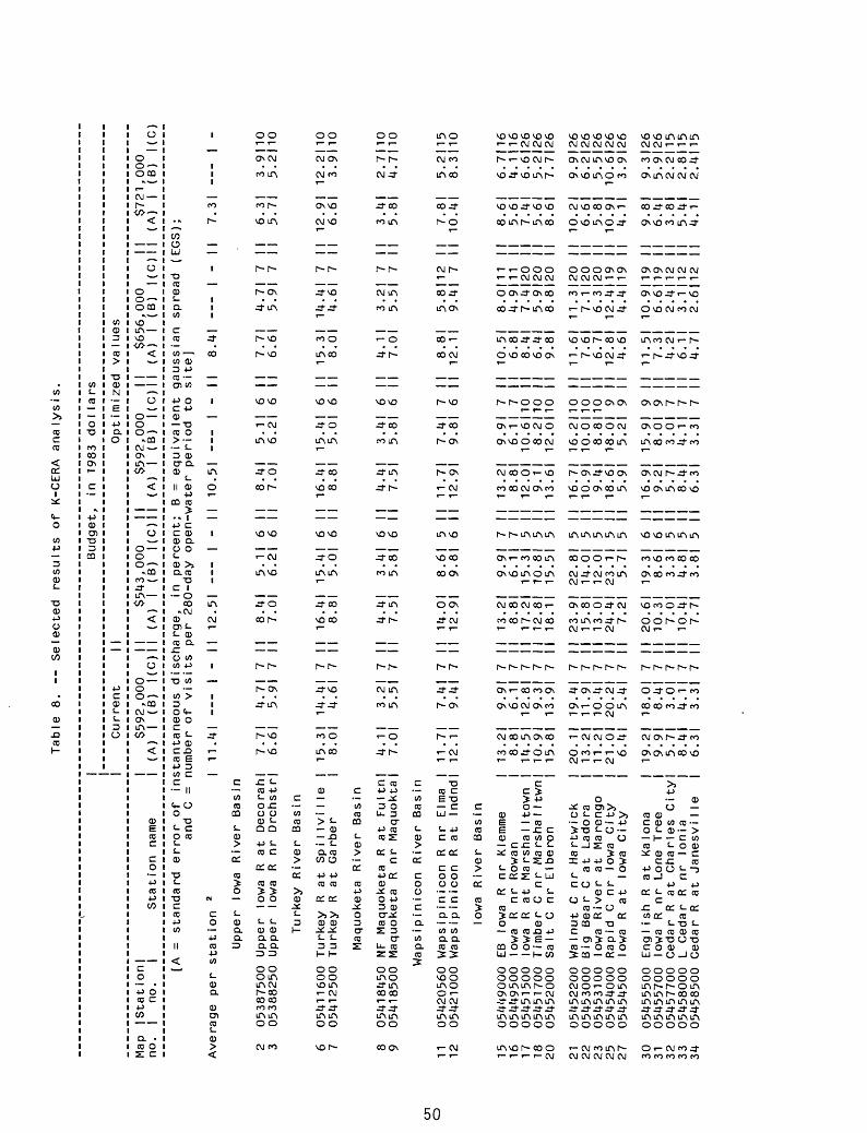
Tabl
e 8.
Selected re
sult
s of
K-
CERA
analysis.
Cu
rre
nt
Bu
dg
et,
in
19
83
do
lla
rs
Op
t im
ized
va
Iue
s
Map
|S
tatio
n|
no
. j
no
. I
Sta
tion
nam
e$
59
2,0
00
II
$543,0
00
II
$592,0
00
II
$6
56
,00
0
||
$721,0
00
(A)
| (B
) |(
C)|
| (A
) I
(B)
|(C
)||
(A)
| (B
) |(
C)||
(A)
I (B
) |(
C)||
(A)
| (B
) |(
C)
[A
= sta
ndard
err
or
of
insta
nta
ne
ou
s
dis
charg
e,
in
perc
ent;
B =
eq
uiv
ale
nt
and
C =
num
ber
of
vis
its
per
28
0-d
ay
op
en
-wa
ter
period
to
Ave
rag
e
per
sta
tio
n
* I
11
.41
Upper
Iow
a R
iver
Ba
sin
12.5
1
I -
fan
sp
rea
d
I
10
.51
I -
I I
8.4
1
| -
gauss
s i te]
11 12 15 16 17 18 20 21 22 23 25 27 30 31 32 33 34
0538
7500
Up
per
Iowa R
at De
cora
hl
7.71
05
3882
50 Up
per
Iowa R
nr Drchstrj
6.6|
Turkey River
Basin
4.71
5.91
8.4
17
.01
5.1
I
6.2
18
.41
7.0
15
.11
6.2
1
05411600
Turk
ey
R a
t S
pillv
ille
|
15
.31
14.4
1
7 05412500
Turk
ey
R a
t G
arb
er
| 8.0
1
4.6
1
716.4
1
15
.41
6
8.8
1
5.0
| 6
16
.41
1
5.4
18.
81
5.01
Ma
qu
oke
ta
Riv
er
Basin
05418450
NF
Ma
qu
oke
ta
R a
t F
ultn
l 05418500
Ma
qu
oke
ta
R n
r M
aq
uo
kta
|
Wapsip
inic
on
Riv
er
Basin
05420560
Wapsip
inic
on
R n
r E
l ma
| 05421000
Wapsip
inic
on
R a
t In
dn
dj
I ow
a R
i ve r
Ba
s i
n
0544
9000
EB Iowa R
nr Klemme
0544
9500
Iowa R
nr Rowan
0545
1500
Io
wa R
at Ma
rsha
l I town
0545
1700
Timber C
nr Ma
rsha
I Itwn
05452000 Salt C
nr El
bero
n
0545
2200
Walnut C
nr Ha
rtwi
ck
0545
3000
Big
Bear
C
at Ladora
0545
3100
Io
wa Ri
ver
at Ma
reng
o 05
4540
00 Rapid
C nr
Io
wa Ci
ty
0545
4500
Io
wa R
at Io
wa Ci
ty
0545
5500
En
glis
h R
at Kalona
0545
5700
Io
wa R
nr Lone Tree
0545
7700
Ce
dar
R at
Charles
City
0545
8000
L Ce
dar
R nr Ionia
0545
8500
Ce
dar
R at JanesviIle
4.1
17
.01
11
.71
1
2.
1|
3.2
| 5
.5I
7.4
I 9.4
I
4.4
I 7.5
I
14
.01
12.9
1
3.41
5.81
8.6
19.8
1
4.41
7.51
11
.71
12
.91
3.41
5.81
7.4
19.8
1
.71
.61
4.71
7
5.91
7
II
15,
II
8,3
| 1
4.4
1
7 01
4.6
1
7
,11
,01
I I
8.8
1
12.1
I
3.2
1
75.5
1
7
5.8
11
2
9.4
| 7
EG
S);
II
7.3
1
II
6.3
1
II
5.7
1
I I
12.9
1II
6.6
1
II
3.4
1
II
5.8
1
I I
7.8
I 1
0.
41
3.9
11
05
.21
10
12.2
110
3.9
11
0
2.7
110
4.7
110
5.2
M5
8.3
110
13.21
9.9
8.81
6.1
14. 51
12
.810
.91
9.3
15.81
13.9
20.1
1 19.4
13.21
11.9
11.21
10.4
21. 01 20.2
6.41
5.4
19.21
18.0
9.9I
8.4
5.7I
3.0
8.4I
4.1
6.31
3.31
7 7 7 7 7 7 7 7 7 7 7 7 7 7 7
13.2
8.8
17.2
12.8
18.1
23.9
15.8
13.0
24.4
7.2
20.6
10.3 7.0
10.4
7.7
9.9I 7
6. 1|
715.31
510.81
515.51
5
22.81
514.01
512.01
523
.1 1
5
5.71 5
19.31
68.6| 6
3.31
5
4.8| 5
3.8|
5
13.21
9.9
8.81
6.1
12.01
10.6
9.11
8.2
13.61
12.0
16.7
1 16.2
10.91
10.0
9.41
8.8
18.61
18.0
5.9I
5.2
16.91
15.9
9.21
8.0
5.71
3.0
8.41
4.1
6.31
3.3
7 7 10 10 10 10 10 10 9 9 9 9 7 7 7
10. 51
8.0111
6.81
4.9111
8.41
7.4120
6.41
5.9120
9.81
8.8120
11.6
1 11.3120
7.61
7.1120
6.71
6.3|20
12.81
12.4119
4.6I
4.4119
11.51
10.9119
7.31
6.6119
4.2|
2.4112
6.1
1 3.1 112
4.71
2.6112
8.61
6.7116
5.6I
4.1116
7.41
6.6126
5.61
5.2126
8.61
7.7126
10.2
1 9.9126
6.61
6.2126
5.81
5.5126
10.9
1 10.6126
4.1|
3.9126
9.81
9.3126
6.41
5.9126
3.81
2.2115
5.41
2.8115
4.11
2.4115

i_CD
O
CO 00ONT
C
0O)
T3
CO
CO
3
CO>
N
E-p
0
Currer
o
oOCQ
O
oOCQ
vo
O
O0
c\?^-ONin
5
o
o .CO
</>
<
o
oCM*
in to-
<
CD£CDC
Co pCO pCO
c o P O CD C p CO
a CO OS c
in in in in in
J- CM co CM J-
j- in in co .
ONinocM J-invo vovo oo
CM CM CM CM CM
O 00 Ovo CM
in invo co oo
. CM . omvo .\O .ON
.....in co oo ^t oo
T
O.3- ON co vo
ON ON 00 ON CM
in in in in in
00 ^t co ON 00
. 00 ON J- CM̂-
O r- 00 CM O
f < O r- in
.....in co oo j- oovo.. d- o
T
O J-ONfOVO
ON ON 00 ON CM
"O T3-* T3 i- >CC i- CO.C ft- O
Ci_ +J 4J CO P JZ S~ 1-T3c o o-c co 3O C ZCO X Xo
U. 1- +J > -P 1 C CD CD CO 1 -P Z
CO CCCC O C -P
(£. X. X. CO .* CO O O > CD 1- O O O CD
CQ CO C£ CC X T3 *-
S- Q5 0 .* CD O > O > 0 CD CO CD u_ c. c. 0 (£. I£CO CO CQ CQ
CO OOOOO > OOOOO
00 ONCM co fOin invo vovoin in in in in ooooo
invo ON o » co co co .3- .3-
ino vooor-r-CM
J-CMOOVO
co in co ^±
CO T- T- CO
d- vo j-in
CM . ON.
00 ON zt 00
coin d- zt
00 r- 00.
J-.^m
.moNm
00 Ztr- zt
Ztr- 00 VO
VOOO VOVO
in invo in
j-^-oj-
invo .m
00 r- r- VO
. 00 00 vo
.0..
00 CM .00
^° (f\ \Q -^°
«^° ^D ^O t""*
vovo .in
COT3 Q)a
O CO oar > oi_ s- co CD CD CD PT3 C CDco CD o a3:OO CD
4J +J i- 03 03 C -P
CD 0:0:0:
o:CO CO CO CO
T3 T3 T3 >CD 0 O Ooo o oooo oooo o mo in j- j- in in
in in in in oooo
CM co ^t m
Skunk River Basin
. ON. .00
CO CM ..r-
J-^..
co CM o in.in invo oo oo
CM J- CM CM .
in ^t in ON.
J" r- CO O CO
vovo .O ON
. .00 oo in
vo o oo in invo. vo ooo
ONOr- 00 O
00 ON ON r- T
in in in in in
oo co zt r- m. 00 00 CM 00
T
OONOO Or- OCM J-r-
.....
VOOCM o inVO. .T- .
r
ONO ON J-co
00 ON ON CM ON
coCO >> co 0 0 CSO i- 3T3 CD
CO CO O C -P 0 J£ O1CO COE co 3< O CO.* O)
CO 3
C C C i- 4J
DC C£ C£ C CO
C C C 3331-.*
CO CO CO T3 3 CD-*
CO CO Z O CO
ooooo ooooo o in in j- oOr- CM CO 3-
in in in in inooooo
VOOOONO r-j- j- j-inin
c
COCQ
O
ca
0co
coo o
vo OO O .
00 CM CM .VO
o^.in
T ^ ON ON ONr-J-J-.VO
r- . .. CM
ON J-vovovo
CM in in ON vo
^t 00 VOOO CO
co invo ON ooT
. r- r- r- .«~ T T
00 .3- ON 00 co
in vovo o ooT r-
VO O CM CM ON
VO.OOr- O
. ON ON ON in
00 ON vo CM co
invo . T- ON
VOVQr- . ON
VO .ONr- CM
.....oo in in oo coin. oo «- oo
vo J" J- J- ON
VO 00 O CM O
-P +J 0)>> T3 ^ T3 -P > CD O i- JO Q Q O P E CO 3 4J 4J S- UJ X CO U_ Q)
P -PCC -P CO CO CO 03 .Q
CO 0oc or 0 en 2:
c co co co t. O 0 O 0 Cc cs: c
cc.O O co O S 2 0 S 0
Q C co co co oQ} Q) U. Q} O Q Q Ld Q CQ
OOOOOomooo in. o moVOVO ONO r- . ..00 00
in in in in inooooo
in in in in in
..ON..
j-oo^-^-vo
vo co OVO 00
r- .CMVOr-
. J-r-VOONT
CM CM . CM CM
j- in in in CM. j- r- . o
T T
co .VO . 00
oo in CM .0
.....
o oo inr- oON in r- ON co
T T
J- ONVO in ONO .CM ON co
in in. in in
oo ON in r- ooONVO'- O zt
T T t
ONOOVO. T-
r- ONCM OVO
.....ooo in r- oON in » ON co
J- ONVO in ON
O .CM ON co
-o- >>i- > -PCi- C- T3 CO +J OO 1- 1- i. (DO P >>O >>C CO CO CO CD CO
CO CQ 0-
C C 1- <- -P C C CD
or or 0:0:0:
co co 0 O C C Cc c o o o ooo ooooo s: s: o o o
CO CO CO CO CO C£ CC. C£ 0 0 QQZ2S
ooooo o mo moCO VO CO Zt VO r- T- CM COCOoo oo oo ooooin in in in in ooooo
00 r- in ON i-mvovovo .
.. ON ON ON
J-OO CM .r-
zt zt ON 00 CM
..CM OON
in in ON ON C\J
CM CMJ- d- J-
CM VO .CM co
mint- OCMCM r-
ONOO oo m =tVOVO r- O CO
CM i-
.....in oo r- ^t ONVOVO .^t CM
CM r-
O 00 co O r-
ON oo . in inCMr-
in in in in in
J-VOOOCM.. ON. co
CM T-
oo co zt oo J-OO ON.VO
.....
in oo r- j- ONvovo . J- CM
CMT-
O 00 CO O r-
ON oo . m in
T3 CO i- Co 0 or >» -P O O d- 0 O S coT3 S CO 1- 0 C£ CO I o: c 0
CD Q 1- P ^ Q C CD -P
4J o: 03 o: o: co
co o co c o: o o o c 0 c0 C o o o o0 OS £2 CO O 1-
CC O CO 3 W5co 0 o o
COCCQU.Q
ooooo ooo J-o o in invo in zt zt in in oo oo oo oo oo ooin in in in inooooo
CM co in VOCM
..voooinr-
ONOO
in CM
CM CM
VOCM
voinVO CO
oooo
.inVOCM
in in. j-
in in
T- O
.CO
00 CM
00 vo
..00 vo
VOCM
ON ON. J-
CO CO > 3E CT 3 CO P O P O0:* p -pCO CD
o: o: co coo o c c0 O2:2:to co0 O QQ
oo oo in in ONO00 ON
mm00
00 00
51
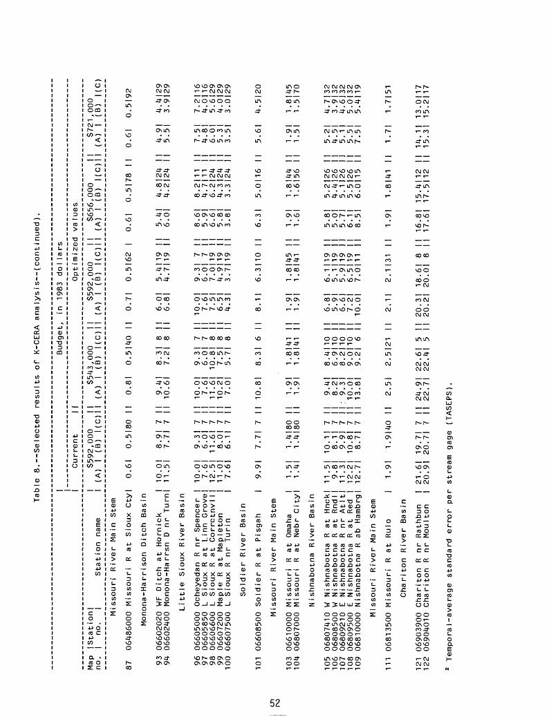
Table
8
. S
ele
cte
d
results of
K-C
ER
A analy
sis
(continued).
Map
no.
iSta
tion
l I
no.
| St
atio
n na
me
Current
1 1
$592
,000
||
(A)
| (B
) |(C)|
1
Budg
et,
$543,000
1 I
(A)
| (B
) |(
C)||
in (A)
1983
$592
I (
do I lars
Opt im
ized
,000
II
B) |(
C)|
|
va I ues
$656
, (A
) I
(000
I I
B)
|(C)
| I
$721
(A)
|,0
00
(B)
I(C)
Mis
souri
Riv
er
Main
S
tem
87
06
48
60
00
M
issouri
Rat
Sio
ux C
tyl
0.6
I 0.5
I80
II
0.8
| 0.5
I40
II
0.7
| 0.5
I62
| 0
.6|
0.5
I78
II
0
.6I
0.5
I92
Monona-H
arr
ison
Ditch
Ba
sin
8.9
I 7
I I
9.4
I 7.7
I 7
I I
10.6
18
.31
8
I I
7.2
| 8
I I
6.0
16.8
15
.41
19
I
I 4
.71
19
I
I
en
ro
93
06
60
20
20
W
F D
itch
at
Horn
ick
I 1
0.
0194
0
66
02
40
0
Mo
no
na
-Ha
rrs
n
D n
r T
urn
j 1
1.5
1
Little
Sio
ux
Riv
er
Basin
96
06605000
Och
eye
dan
R n
r S
pence
r |
10. 0|
97
06605850
L S
iou
x
R a
t L
inn
G
rovel
98
06606600
L S
ioux
R a
t C
orr
ctn
vl
I I
99
06607200
Ma
ple
R
at
Maple
ton
I10
0 0
66
07
50
0
L S
ioux
R n
r T
urin
I
So
Id ier
Riv
er
Basin
101
06608500
Sold
ier
R a
t P
isgah
I 9.9
I 7
.7I
7 II
10.8
1
8.3
1
6 II
8.1
| 6
.3|1
0
Mis
souri
Riv
er
Ma
in
Ste
m
5.41
6.0
14
.81
24
I
I 4.2
|24
I|4
.91
5.5
1
6.3
| 5.0
116
103
104
105
106
107
108
109
06610000
06807000
06807410
06808500
06809210
06809500
06810000
Miss
ouri
R
at Om
aha
IMi
ssou
ri
R at Nebr Ci
tyl
Nish
nabo
tna
River
Basi
n
W Ni
shna
botn
a R
at Hnckl
W Ni
shna
botn
a R
at Rn
d I I
E Ni
shna
botn
a R
nr Atltl
E Ni
shna
botn
a R
at Re
d |
Nishnabotna
R ab
Ha
mbrg
j
1.51
1.41
11.5
19.81
11.3
112.21
12.71
1. 1 .
10. 8. 9. 10. 8.
4 I 80
4 I 80
11 7
11
791
7
81 7
71 7
1.91
1.91
9.41
8.2|
: 9.31
10.01
13.81
1.81
41
I1.
8141
I
8. 4110
16.9110
I8.2110
I9.0110
I9.2| 6
I
1.91
1.91
6.81
5.91
6.61
7.21
10.01
1 1 6 5 5 6 1
.814
5.8141
.111
9.1119
.9119
.5M9
.011
1
4.4
|29
3.9
I 29
10.01
9.31 7
II 10
.01
9.31
7 1
7.61
6.01
7
1 1
7.61
6.01
7 1
12.51
11.61
7 1
1 11
.61
10.81
8 1
11.01
8.01
7
1 1
10.21
7.51 8
1 7.61
6.1
1 7
||
7.01
5.71 8
1
10.01
9.31 7
7.61
6.01 7
7.51
7.0119
6.5I
4.9119
4.3I
3.7119
8.6I
8.2111
5.9I
4.7111
6.6I
6.2I24
5.8I
4.3I24
3.8I
3.3I24
7.5I
7.2116
4.8I
4.0116
6.0|
5.6I29
5.3I
4.0I29
3. 5 I
3.0
I 29
5.6
| 4.5
I20
1.91
1.61
5.81
5.
01
5.71
6.11
8.
51
1.8144
1.6156
5.2126
4.4126
5.1126
5.5126
6.0115
I 1.
91
1 1.51
1 5.2|
1 4.51
1 5.
11
1 5.51
1 7.
51
1.8145
1.5170
4.7132
3.9132
4.6132
5.0132
5.4|19
Mis
souri
Riv
er
Main
S
tem
111
06813500
Mis
souri
R a
t R
ulo
I
1.9
1
1.9
14
0
II
2.5
1
2.5
12
1
||
2.1
| 2.1
131
II
1.9
1
1.8
141
II
1.7
| 1.7
151
Ch
arito
n
Riv
er
Basin
121
06
90
39
00
C
ha
rito
n
R n
r R
ath
bu
n12
2 06904010
Ch
arito
n
R n
r M
ou
lto
nI
21
.61
19.7
1
7 II
24
.91
22.6
1
5 II
2
0.3
1
18
.61
8
II
16.8
1
15.4
112
||
14.1
| 13.0
117
| 20. 9
l 20. 7
l 7
II
22. 7|
22. 4|
5 II
20. 2|
20. 0|
8 ||
17
.61
17.5
112
||
15
.31
15.2
|17
Te
mp
ora
I-a
vera
ge
sta
ndard
e
rro
r per
str
ea
m
gage
(TA
SE
PS
).
Kalman-filtering techniques were used to develop a flexible and expedient model describing the variability of discharges and shifts of the stage-discharge relations of alluvial rivers. An explanation of the method, a description of the model, and its applications have been described by Kitanidis and others (1984). Briefly, they found that the error in the stage-discharge relation was a function of water temperature. The stage-discharge relationship changes as the stream- bed form changes. The bed form relates to the ability of the water to suspend the sediment which is related to the water temperature. During winter, the bed form is smooth and during summer, the bed form has large, moving dunes. Therefore, for a given stage, the discharge is greater during the winter when the stream bed is smooth. The K-CERA analysis predicts the next day's discharge and the standard error. When the error exceeds the accuracy required, a discharge measurement is scheduled to adjust the next day's analysis. This is a good example of the need and importance of good record and accurate data for project operations.
The model mentioned above was used in simulations designed to evaluate a number of various sampling strategies. From these simulations it was concluded that the optimal approach would be to adopt a "real-time" stream-gaging strategy that will allow the District to maximize quality of data with a given budget. To accomplish this approach the following steps need to be taken:
1. Install telemetering equipment with automatic data-transfer capability in each of the gaging stations. Telemetering equipment has been installed.
2. Provide the Council Bluffs field headquarters with a microcomputer to access the model and the site-specific model parameters on line, and with the capability of interphasing with the telemetering equipment.
3. Develop computer programs that will enable the microcomputer to query each of the stations for pertinent data at 6-hour intervals and store them in memory.
4. Develop computer programs that will operate the model at the end of each day. The estimated discharge and its corresponding standard error of estimate for each station will be printed daily.
Based on the magnitude of current estimation error, the hydrologist in charge would decide if a measurement at a particular station on the river is needed that day or soon after.
Summary of the Third Phase of Analysis
Results of the K-CERA analysis are:
1. Visits to gaging stations need to be maintained at 7 per open-water period (280 days) and 3 per winter period. By optimizing the gaging schedule, the average standard error would be decreased from 11.4 to 10.5 percent with the same budget of $592,000.
2. The amount of funding for stations with accuracies that are not acceptable for the data uses need to be renegotiated with the data users.
3. The K-CERA analysis needs to be made whenever new stations are added and sufficient information about the characteristics of the new stations has been obtained.
53
4. Techniques for decreasing the probabilities of missing record, for example increased use of satellite relay of data and updated equipment need to be explored and evaluated as to their cost-effectiveness in providing streamf low information.
5. The "traveling hydrographer" analysis needs to be made each year or whenever new field schedules are needed to optimize field operation.
6. Data collection of other hydrologic parameters needs to continue in the streamflow data program. The K-CERA analysis shows a significant savings in travel time and route cost for the present programs of crest- stage stations and observation wells.
7. The Iowa District needs to take the necessary steps to implement the "real-time" stream-gaging strategy for the stations on the Missouri River. Implementing this strategy would be beneficial not only to Iowa but nationwide. The Geological Survey needs to demonstrate to cooperators and administrators that our agency is determined to optimize the operation of our networks, and has the capability of using the tools currently available.
SUMMARY
Currently (1983), there are 110 continuous streamflow stations, being operated in Iowa at a cost of $592,000. Additional stations in the regular surface water program include 4 reservoir, 4 lake, 3 stage only and 1 miscellaneous station that are budgeted separately. Seventeen separate sources of funding contribute to the continuous streamflow program and six separate uses were identified. The data use for all of the stations are necessary as defined. Twelve of the 51 stations classified as "regional hydrology" are not funded for other uses. These stations would be the only candidates for discontinuance when sufficient definition of transferable hydrologic data is obtained. Emphasis needs to be placed on expanding the streamflow-data-collection program to include the 21 ungaged streams with drainage areas between 200 and 400 mi 2 .
No daily discharges can be estimated accurately enough by using regression- correlation or flow-routing techniques. One study in the Skunk River basin indicates a need for a station downstream from the water-treatment plant at Ames if more accurate streamflow data are needed for plant operation. Knowledge from the flow-routing studies will improve estimation or reconstruction of lost record at a station in the set of routing stations. Although the results of the alternative method study for station 42 (Cedar River at Waterloo) and station 56 (Des Moines River at Fort Dodge) are encouraging if the models are calibrated to their full potential, the data use for these stations require a greater degree of accuraccy than that possible from the present models.
It was shown that the current operating budget for 110 streamflow sites required a budget of $592,000. The temporal average standard error would be improved from 11.4 percent for current practice to 10.5 percent if the gaging schedule was optimized. The average standard error would be improved to 8.4 percent with a 10 percent increase to the present budget to $656,000 and to 4.2 percent with a budget of $1,235,000.
A major component of the error in streamflow records is caused by loss of gage-height record because of malfunctions of sensing and recording equipment. Upgrading of equipment, adding telemetry, and frequent monitoring of instrument operation would decrease the loss of record.
54

Cost-effective studies of the stream-gaging program need to be continued. Future studies also will be required because of changes in demands for streamflow information. The optimum ratio of discharge measurements, site visits, and accuracy of data need to be determined.
55
REFERENCES CITED
Benson, M. A., and Carter, R. W., 1973, A national study of the streamflow data-collection program: U.S. Geological Survey Water-Supply Paper 2028, 44 p.
Bowie, J. E., and Petri, L. R., 1969, Travel of solutes in the lower Missouri River: U. S. Geological Survey Hydrologic-lnvest-igations Atlas HA-332.
Burmeister, I. L., 1970, The streamflow data program in Iowa: U. S. Geological Survey open-file report, 82 p.
Draper, N. R., and Smith, H., 1966, Applied regression analysis (2d ed.): New York, John Wiley, 709 p.
Fontaine, R. A., Moss, R. E., Smath, J. A., and Thomas, W. O., 1983, Cost effectiveness of the stream-gaging program in Maine: U. S. Geological Survey Survey Open-File Report, 81 p.
Gelb, A., ed., 1974, Applied optimal estimation: Cambridge, Mass., The Massachusetts Institute of Technology Press, 374 p.
Gilroy, E. J., and Moss, M. E., 1981, Cost-effective stream-gaging strategies for the Lower Colorado River Basin: U.S. Geological Survey Open-File Report 81-1019, __p.
Hutchison, N. E., 1975, WATSTORE User's guide, volume 1: U.S. Geological Survey Open-File Report 75-426, __p.
Keefer, T. N., 1974, Desktop computer flow routing: American Society of Civil Engineers Proceedings, Journal of the Hydraulics Division, v. 100, no. HY7, p. 1047-1058.
Keefer, T. N., and McQuivey, R. S., 1974, Multiple linearization flow routing model: American Society of Civil Engineers Proceedings, Journal of the Hydraulics Division, v. 100, no. HY7, p. 1031-1046.
Kitanidis, P., Lara, O. G., and Lane, R. W., 1984, Evaluation of the efficiency of streamflow data-collection strategies for alluvial rivers: U. S. Geological Survey Water-Supply Paper __, [in press],
Kleinbaum, D. G., and Kupper, L. L., 1978, Applied regression analysis and other multivariable methods: North Scituate, Mass., Duxbury Press, 556 p.
Lara, O. G., 1973, Floods in Iowa: Technical manual for estimating their magnitude and frequency: Iowa Natural Resources Council Bulletin No. 11, 56 p.
________, 1979, Annual and seasonal low-flow characteristics of Iowa streams:U. S. Geological Survey Open-File Report 79-555, 507 p.
57
Larimer, O. J., 1957, Drainage areas of Iowa streams: Iowa Highway ResearchBoard Bulletin No. 1, 437 p. (reprinted 1974).
Mitchell, W. D., 1972, Effect of reservoir storage on peak flow: U.S. GeologicalSurvey Water-Supply Paper 1580, p. C1-C25.
Moss, M. E., and Gilroy, E. J., 1980, Cost-effective stream-gaging strategies for the Lower Colorado River Basin: U.S. Geological Survey Open-File Report 80-1048, 111 p.
Riggs, H. C., 1973, Regional analysis of streamflow characteristics: U.S. Geological Survey Techniques of Water-Resources Investigations, Book 4, Chapter B3, 15 p.
Sauer, V. B., 1973, Unit response method of open-channel flow routing: American Society of Civil Engineers Proceedings: Journal of the Hydraulics Division, v. 99, no. HY1, p. 179-193.
Thomas, D. M., and Benson, M. A., 1970, Generalization of streamflow chacteristics from drainage-basin characteristics: U.S. Geological Survey Water-Supply Paper 1975, 55 p.
U.S. Geological Survey, 1983, Water-Resources data for Iowa, water year 1982: U.S. Geological Survey Water-Data Report IA-82-1, 262 p.
58
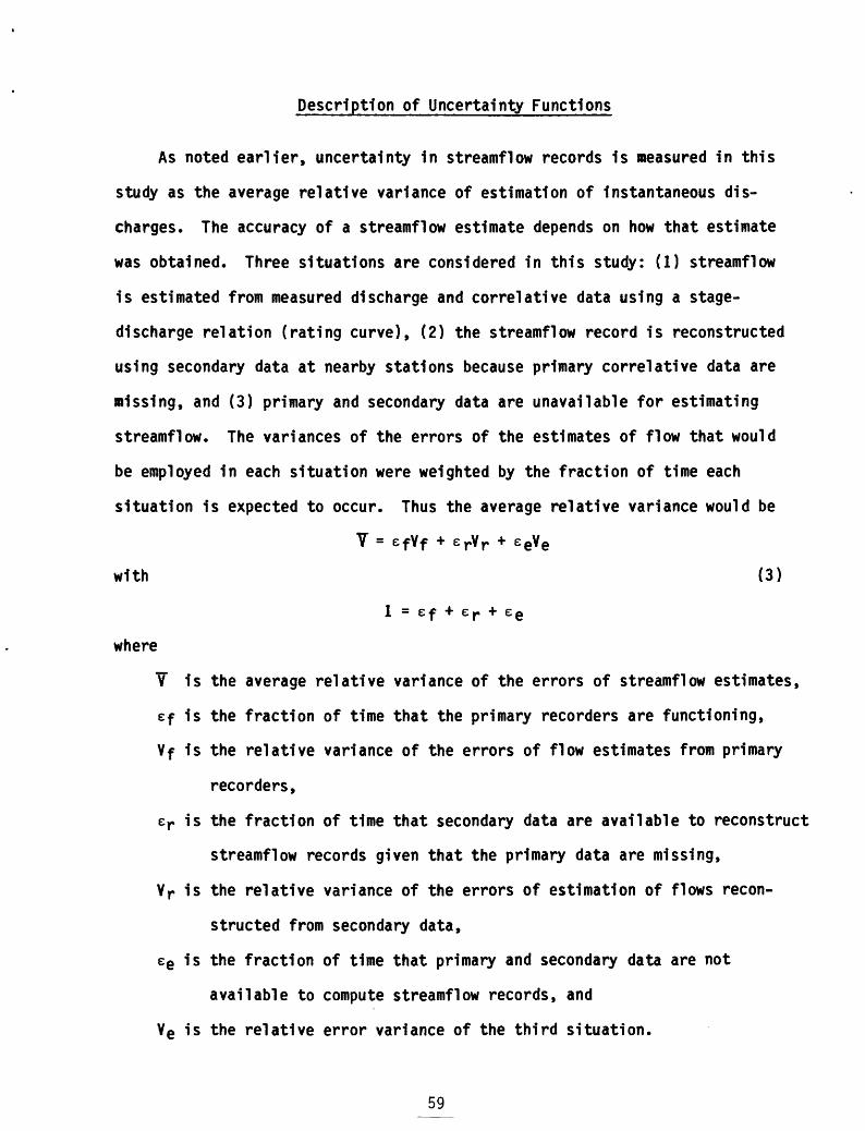
Description of Uncertainty Functions
As noted earlier, uncertainty in streamflow records is measured in this
study as the average relative variance of estimation of instantaneous dis
charges. The accuracy of a streamflow estimate depends on how that estimate
was obtained. Three situations are considered in this study: (1) streamflow
is estimated from measured discharge and correlative data using a stage-
discharge relation (rating curve), (2) the streamflow record is reconstructed
using secondary data at nearby stations because primary correlative data are
missing, and (3) primary and secondary data are unavailable for estimating
streamflow. The variances of the errors of the estimates of flow that would
be employed in each situation were weighted by the fraction of time each
situation is expected to occur. Thus the average relative variance would be
Y = efVf + e rY r + e eve
with (3)
1 = ef + e r + e e
where
Y is the average relative variance of the errors of streamflow estimates,
ef is the fraction of time that the primary recorders are functioning,
Vf is the relative variance of the errors of flow estimates from primary
recorders,
er is the fraction of time that secondary data are available to reconstruct
streamflow records given that the primary data are missing,
Y r is the relative variance of the errors of estimation of flows recon
structed from secondary data,
ee is the fraction of time that primary and secondary data are not
available to compute streamflow records, and
Ve is the relative error variance of the third situation.
59

The fractions of time that each source of error is relevant are functions
of the frequencies at which the recording equipment 1s serviced.
The time T since the last service visit until failure of the recorder
or recorders at the primary site is assumed to have a negative-exponential
probability distribution truncated at the next service time; the distribution's
probability density function is
f(t) = ke-kt/d-e-ks) (4)
where
k is the failure rate 1n units of (day)'1 ,
e 1s the base of natural logarithms, and
s is the Interval between visits to the site in days.
It is assumed that, If a recorder fails, it continues to malfunction until
the next service visit. As a result,
e f = (l-e-ks )/(ks) (5)
(Fontaine and others, 1983, eq. 21).
The fraction of time e e that no records exist at either the primary or
secondary sites can also be derived assuming that the time between failures
at both sites are independent and have negative exponential distributions with
the same rate constant. It then follows that
ee = 1 - [2(l-e-ks ) + 0.5(l-e-2ks)]/(ks)
(Fontaine and others, 1983, eqs. 23 and 25).
Finally, the fraction of time e r that records are reconstructed based on
data from a secondary site is determined by the equation
= [(1-e-ks) + 0.5(l-e-2ks)]/( ks )
60

The relative variance, Yf, of the error derived from primary record
computation is determined by analyzing a time series of residuals that are
the differences between the logarithms of measured discharge and the rating
curve discharge. The rating curve discharge is determined from a relationship
between discharge and some correlative data, such as water-surface elevation
at the gaging station. The measured discharge is the discharge determined by
field observations of depths, widths, and velocities. Let qj(t) be the true
instantaneous discharge at time t and let qg(t) be the value that would be
estimated using the rating curve. Then
x(t) = In oj(t) - In qR (t) = In Coj(t)/qR(t)] (7)
is the instantaneous difference between the logarithms of the true discharge
and the rating curve discharge.
In computing estimates of streamflow, the rating curve may be continually
adjusted on the basis of periodic measurements of discharge. This adjustment
process results in an estimate, qc (t), that is a better estimate of the
stream's discharge at time t. The difference between the variable x(t),
which is defined
x(t) = In qc (t) - In qR (t) (8)
and x(t) is the error in the streamflow record at time t. The variance of
this difference over time is the desired estimate of Yf.
Unfortunately, the true instantaneous discharge, qj(t), cannot be
determined and thus x(t) and the difference, x(t) - x(t), cannot be determined
as well. However, the statistical properties of x(t) - x(t), particularly
its variance, can be inferred from the available discharge measurements. Let
the observed residuals of measured discharge from the rating curve be z(t) so
that
61

z(t) * x(t) + v(t) * In qm(t) - In qR (t) (9)
where
v(t) 1s the measurement error, and
In qm(t) 1s the logarithm of the measured discharge equal to In qj(t)
plus v(t).
In the Kalman-fllter analysis, the z(t) time series was analyzed to
determine three site-specific parameters. The Kalman filter used 1n this
study assumes that the time residuals x(t) arise from a continuous first-
order Markovian process that has a Gausslan (normal) probability distribution
with zero mean and variance (subsequently referred to as process variance)
equal to p. A second Important parameter 1s $, the reciprocal of the correl
ation time of the Markovian process giving rise to x(t); the correlation
between x(t}) and x(t£) 1s exp[-$|ti-t2|]» Fontalne and others (1983) also
define q, the constant value of the spectral density function of the white
noise which drives the Gauss-Markov x-process. The parameters, p, q, and $ are
related by
Yar[x(t)] = p = q/(23) (10)
The variance of the observed residuals z(t) 1s
Yar[z(t)] = p + r (11)
where r 1s the variance of the measurement error v(t). The three parameters,
p, e, and r, are computed by analyzing the statistical properties of the z(t)
time series. These three site-specific parameters are needed to define this
component of the uncertainty relationship. The Kalman filter utilizes these
three parameters to determine the average relative variance of the errors of
estimation of discharges as a function of the number of discharge measure
ments per year (Moss and Gllroy, 1980).
62

If the recorder at the primary site fails and there are no concurrent
data at other sites that can be used to reconstruct the missing record at the
primary site, there are at least two ways of estimating discharges at the
primary site. A recession curve could be applied from the time of recorder
stoppage until the gage was once again functioning or the expected value of
discharge for the period of missing data could be used as an estimate. The
expected-value approach is used in this study to estimate V e , the relative
error variance during periods of no concurrent data at nearby stations. If
the expected value is used to estimate discharge, the value that is used
should be the expected value of discharge at the time of year of the missing
record because of the seasonality of the streamflow processes. The variance
of streamflow, which also is a seasonally varying parameter, is an estimate
of the error variance that results from using the expected value as an esti
mate. Thus the coefficient of variation squared (Cv ) 2 is an estimate of the
required relative error variance V e . Because Cv varies seasonally and the
times of failures cannot be anticipated, a seasonally averaged value of Cv is
used:
LL f pi1.365 iiiVM1
11/2
rv - ii l f-il i (12)
where
oj is the standard deviation of daily discharges for the i tn day of the
year,
y^ is the expected value of discharge on the 1*n day of the year, and
f£v )2 is used as an estimate of Ve .
The variance V r of the relative error during periods of reconstructed
streamflow records is estimated on the basis of correlation between records
63

at the primary site and records from other gaged nearby sites. The correlation
coefficient pc between the streamflows with seasonal trends removed at the
site of interest and detrended streamflows at the other sites Is a measure of
the goodness of their linear relationship. The fraction of the variance of
streamflow at the primary site that is explained by data from the other sites
is equal to p c2 . Thus, the relative error variance of flow estimates
at the primary site obtained from secondary Information will be
V r
Because errors in streamflow estimates arise from three different sources
with widely varying precisions, the resultant distribution of those errors may
differ significantly from a normal or log-normal distribution. This lack of
normality causes difficulty in interpretation of the resulting average esti
mation variance. When primary and secondary data are unavailable, the relative
error variance Ve may be very large. This could yield correspondingly large
values of V" in equation (3) even if the probability that primary and secondary
information are not available, e e , is quite small.
A new parameter, the equivalent Gausslan spread (EGS), is introduced
here to assist in interpreting the results of the analyses. If it is assumed
that the various errors arising from the three situations represented 1n
equation (3) are log-normally distributed, the value of EGS was determined
by the probability statement that
Probability [e-EGS £ (qc (t) / qj(t)) _< e*EGS ] = 0.683 (14)
Thus, if the residuals In qc(t) - In qj(t) were normally distributed, (EGS) 2
would be their variance. Here EGS is reported in units of percent because
EGS is defined so that nearly two- thirds of the errors in instantaneous
streamflow data will be within plus or minus EGS percent of the reported
values.
64

Relationship of visit frequency to lost record
by M. E. Moss
It is assumed that, if the sensing or recording equipment at a stream gage fails between service visits to the gage, the time, T, from the last service visit until the failure has a conditional probability distribution that is defined by the truncated negative exponential family
__ \f T If C!
f t Ft. I / / 4 JN.O \ T = ke /(1-e )
where s is the interval between visits and k is a parameter of the family of probability distributions ( 1/k is the average time to failure). It also is assumed that the recorder continues to malfunction from the instant of failure until the next service visit. Thus, the fraction of time, £f, that the gage can be expected to function properly is
e f = 1 - E[d]/s
where E[*] is the expected value of the random variable contained in the brackets and d is the downtime of the recorder between visits. Downtime is defined
I'S-T if a failure occurs, d = i
(0 if no failure occurs
as is shown in figure 16.
The expected value of downtime is
E[d] = / (S-T) f T dT
which when evaluated results in
E[d] = (ks + e~ks-1
Substituting equation 20 into equation 17 and simplifying result in
e f = (1-e~ks )/ks.
The fraction of time, e e , that no record is available at the station oJ interest and no record is available from an auxiliary site to reconstruct at the station of interest (both caused by equipment failures) is obtainable from a bivariate application of equation 16. If it is assumed that the probability distributions of failure times are identical and independent at the primary and auxiliary sites and that the primary and auxiliary sites are serviced at about the same times, e e can be evaluated as follows.
65

s
d
d
= Time to failure= Service interval= Down time (missing stage record)
= s T
^ Time of the nth visit
LUCD<CO
T-
+ 1TIME
Figure 10. Nomogram showing definition of downtime for a single station.
66

The concurrent downtime, d2 , °f both stations is defined
if both stations fail,
{min (s-Ta , s-T) i
0 otherwise
where Ta is the time to failure at the auxiliary site. The case in which s-Ta is the minimum and equals d2 *- s shown in figure 17. The value of ee can be defined in terms of d2 as
ee = E[d2 ]/s.
The expected value of concurrent downtime is
fs fsE[d2 ] =/ (S-T) P[T C _< T] fT dT +1 (S-T C ) P[T _< T C ] f T dT
Jo «/o c c
where P[*] is the probability of the event contained within the brackets occurring. Evaluation of equation 24 under the given assumptions results in
E[d0 ] = s - ^- (1-e~ks ) - L (1-e~2ks )z k 2k
which can be substituted into equation 23 to obtain ee .
Because £f, ee , and e r are mutually exclusive and all encompassing
ef + ee + er = 1.
From equation 26, er can be defined
er = 1 - e f - ee .
67

LUCD<CO
-TV
Auxiliary record
Primary record
n+1
TIME
Figure 11. Diagram showing definition of joint downtime for a pair of stations.
68