European Spatial Data Research

Tree Extraction

by Harri Kaartinen and Juha Hyyppä

Official Publication No 53

June 2008

The present publication is the exclusive property of European Spatial Data Research

All rights of translation and reproduction are reserved on behalf of EuroSDR. Published by EuroSDR Printed by Gopher, Amsterdam, The Netherlands

EUROPEAN SPATIAL DATA RESEARCH PRESIDENT 2008 – 2010: Antonio Arozarena, Spain VICE-PRESIDENT 2005 – 2009: Christian Heipke, Germany SECRETARY-GENERAL: Kevin Mooney, Ireland DELEGATES BY MEMBER COUNTRY: Austria: Michael Franzen Belgium: Ingrid Vanden Berghe Croatia: Željko He�imovi�; Ivan Landek Cyprus: Christos Zenonos; Michael Savvides Denmark: Joachim Höhle; Nikolaj Veje Finland: Risto Kuittinen; Juha Vilhomaa France: Raphaéle Heno; Jean-Philippe Lagrange Germany: Dietmar Grünreich; Günter Nagel; Dieter Fritsch Hungary: Arpad Barsi Iceland: Magnús Guðmundsson; Eydís Líndal Finnbogadóttir Ireland: Colin Bray, Ned Dwyer Italy: Carlo Cannafoglia Netherlands: Jantien Stoter; Aart-jan Klijnjan Norway: Jon Arne Trollvik; Ivar Maalen-Johansen Spain: Antonio Arozarena, Francisco Papí Montanel Sweden: Stig Jönsson; Anders Östman Switzerland: Francois Golay; André Streilein-Hurni United Kingdom: Malcolm Havercroft; Jeremy Morley COMMISSION CHAIRPERSONS: Sensors, Primary Data Acquisition and Georeferencing: Michael Cramer, Germany Image Analysis and Information Extraction: Juha Hyyppä, Finland Production Systems and Processes: André Streilein-Hurni, Switzerland Data Specifications: Keith Murray, United Kingdom Network Services: Mike Jackson

OFFICE OF PUBLICATIONS: Bundesamt für Kartographie und Geodäsie (BKG) Publications Officer: Andreas Busch Richard-Strauss-Allee 11 60598 Frankfurt Germany Tel.: + 49 69 6333 312 Fax: + 49 69 6333 441 CONTACT DETAILS: Web: www.eurosdr.net President: president@eurosdr.net Secretary-General: secretary@eurosdr.net Secretariat: admin@eurosdr.net EuroSDR Secretariat Faculty of the Built Environment Dublin Institute of Technology Bolton Street Dublin 1 Ireland Tel.: +353 1 4023933 The official publications of EuroSDR are peer-reviewed.

EuroSDR / ISPRS Project

Commission II “Tree Extraction”

Final Report

Report by Harri Kaartinen and Juha Hyyppä

Finnish Geodetic Institute, Masala, Finland

6

TABLE OF CONTENTS

ABSTRACT ................................................................................................................ 7�

1� INTRODUCTION ................................................................................................ 7�

2� MATERIAL .......................................................................................................... 9�2.1� Test Sites ............................................................................................................................... 9�2.2� Delivered Data ...................................................................................................................... 9�2.3� Reference Data.................................................................................................................... 10�2.4� Produced 3D-models .......................................................................................................... 11�

3� METHODS.......................................................................................................... 12�3.1� Methods Used by Participants ............................................................................................ 12�

3.1.1� Definiens ................................................................................................................ 12�3.1.2� FOI ......................................................................................................................... 15�3.1.3� Pacific Forestry Centre .......................................................................................... 16�3.1.4� University of Hannover ......................................................................................... 16�3.1.5� Joanneum Research ............................................................................................... 17�3.1.6� Metla ...................................................................................................................... 18�3.1.7� Norwegian Forest Research Institute and University of Life Sciences .................. 18�3.1.8� National Ilian University ....................................................................................... 20�3.1.9� Texas A&M University ......................................................................................... 22�3.1.10� University of Zürich .............................................................................................. 26�3.1.11� Progea Consulting and Agricultural University of Cracow ................................... 29�3.1.12� University of Udine ............................................................................................... 29�

3.2� Methods for Accuracy Evaluation of Participants’ Tree Models ........................................ 31�3.3� Examples of Extracted Models ........................................................................................... 32�

4� RESULTS ............................................................................................................ 35�4.1� Amount of Extracted Trees ................................................................................................. 35�4.2� Tree Location Accuracy ...................................................................................................... 36�4.3� Tree Height Accuracy ......................................................................................................... 39�4.4� Crown Base Height Accuracy ............................................................................................. 42�4.5� Crown Delineation Accuracy .............................................................................................. 44�4.6� Tree Species Classification ................................................................................................. 47�

5� DISCUSSION AND CONCLUSIONS ............................................................. 47�

ACKNOWLEDGMENTS ....................................................................................... 49�

REFERENCES ......................................................................................................... 50�

7

Abstract

The objective of the EuroSDR/ISPRS Tree Extraction project was to evaluate the quality, accuracy, and feasibility of automatic or semi-automatic tree extraction methods based on high-density laser scanner data and digital image data. Data sets from two test sites were delivered to the twelve participants of the project. For each test site the following data were available and could be downloaded from the FGI ftp-site: aerial images, camera calibration and image orientation information, ground control point coordinates and jpg-images of point locations, laser scanner data with three different pulse densities, digital terrain model and a training data set. In this report the test sites used, data sets and the reference data are described. The tree extraction methods used by the participants and methods used in accuracy evaluation are explained in this report. The produced tree models are depicted and analysed with respect to tree location, tree height, crown base height and crown delineation accuracy. Finally, a discussion and conclusions chapter summarise the results of the project. Surprisingly, results show that the extraction method is the main factor on the achieved accuracy. When the laser point density increases from two points to eight points per m2, the improvement in crown base height and crown delineation accuracy is marginal but in the case of some methods the accuracy of the tree location and especially the tree height determination improves. The low number of hybrid models based on both the laser data and aerial image produced by the partners implies that integration of laser and aerial image is in its early stages.

1 Introduction

The background to the use of laser scanning for forest measurement stems from the use of laser profilers for forests. Laser profilers were used in forest studies from around 1980 (Solodukhin et al. 1977, Nelson et al. 1984, Schreier et al. 1985, Aldred and Bonnor 1985, Maclean and Krabill 1986, Bernard et al. 1987, Currie et al. 1989). They gave the background to methods nowadays known as area-based methods or distribution-based methods, where features and predictors are assessed from the laser-derived surface models and canopy height point clouds, which are directly used for forest parameter estimation, typically using regression, non-parametric or discriminant analysis, of the mean tree height, basal area and volume (e.g. Lefsky et al. 1999, Magnussen et al. 1999, Means et al. 1999, Næsset 1997a,b, Næsset and Økland 2002, Næsset 2002, Lim et al. 2002, Hopkinson et al. 2006, Maltamo et al. 2006b). Examples of the accuracy of techniques based on canopy height distribution can be found in Næsset et al. (2004). The proposed linear approach in Hollaus (2006) based, for example, on original work of Nelson et al. (1984, 1988) and adapted from 2D canopy profiles to 3D canopy heights showed that, for Airborne Laser Scanner (ALS) data with varying properties, robust and reliable results of high accuracies (e.g. coefficient of determination R2 = 0.87, standard deviation of the stem volume residuals derived from a cross-validation is 90.0 m3/ha) can be achieved. Due to the simplicity of this linear model a physically explicit connection between the stem and the canopy volume is available.

Recent developments in the computer analysis of high spatial resolution images and increases in pulse repetition frequency (PRF) of laser scanner from 2 kHz (in 1994) to 200 kHz (in 2007) have led to the semi-automated production of laser-assisted forest inventories based on individual tree crown information. The methods used in laser scanning can utilize the methods already developed using high and very high resolution aerial imagery. Additionally, in laser scanning it is possible to improve the image based approaches by utilizing the powerful ranging algorithms and knowledge-based approaches (e.g. we know the tree height and we can roughly estimate the size of the crown). Hyyppä and Inkinen (1999), Friedlaender and Koch (2000) and Ziegler et al. (2000) demonstrated the

8

individual-tree-based forest inventory using laser scanner tree finding with maxima of the Canopy Height Model (CHM, also designation Digital Canopy Model, DCM, is used) and segmentation for edge detection. Hyyppä and Inkinen (1999) also presented the basic LiDAR-based individual tree crown approach in which, for individual trees, location, tree height, crown diameter and species are derived using laser, possibly in combination with aerial image data, especially for tree species classification, and then other important variables, such as stem diameter, basal area and stem volume, are derived using existing models. The methods were tested in Finnish, Austrian and German coniferous forests and 40 to 50% of the trees could be correctly segmented (Hyyppä et al. 2001). Persson et al. (2002) improved the crown delineation and could link 71% of the tree heights with the reference trees. Other attempts to use Digital Surface Model (DSM) or CHM image or point clouds for individual tree crown (ITC) isolation or crown diameter estimation have been reported by e.g. Anderssen et al. (2002), Brandtberg et al. (2003), Leckie et al. (2003), Morsdorf et al. (2003), Straub (2003a), Popescu et al. (2003), Wack et al. (2003), Pitkänen et al. (2004), Sohlberg et al. (2006), Tiede and Hoffmann (2006) and Falkowski et al. (2006).

Laser scanning is increasingly becoming a core data set for mapping authorities and the pulse density of laser scanning is increasing constantly. In addition to forest inventory, tree information is used, for example, in flight obstacle mapping, power line mapping, real estate visualization and mapping, and telecommunication planning. The results obtained for individual tree extraction have varied significantly from study to study (percentage of correctly delineated trees has ranged from 40 to 93 %. With regard to the methods, there is a trend towards more efficient use of the point cloud data, rather than segmenting pure laser-derived DSMs. It is not known how much of this variation is caused by the methods and how much by forest conditions.

A high synergy exists between the high-resolution optical imagery and laser scanner data for extracting forest information. Laser data provides accurate height information, which is missing in single optical images, and also supporting information on the crown shape depending on the applied pulse density, whereas optical images provide more detail about spatial geometry and colour information usable for classification of tree species and health. Both provide information on crown shape and size. Even though these aspects have been known for quite a long time, a small amount of research has been published on the topic (e.g. St-Onge, 1999; Hyyppä et al., 2000; St-Onge and Achaichia, 2001; Leckie et al., 2003; Persson et al. 2004, Hyyppä et al. 2005, Suarez et al. 2005, Maltamo et al., 2006b).

The objective of the EuroSDR/ISPRS Tree Extraction project was to evaluate the quality, accuracy, and feasibility of automatic or semi-automatic tree extraction methods based on high-density laser scanner data and digital image data. The sub-objectives included

- How much variation is caused in the tree extraction by the methods employed. - How much is the affect of the point density of laser data on tree extraction. - How much can the results be improved by integrating laser scanner data and aerial data.

Twelve partners from USA, Canada, Norway, Sweden, Finland, Germany, Austria, Switzerland, Italy, Poland and Taiwan participated in the test covering global knowledge of tree extraction. Participants were requested to extract trees using the given material. They were allowed to use any method and data combination. Participants were asked to provide, for each tree, the following information (as many attributes as it is possible):

- Tree location (x,y coordinates of the supposed centre of the trunk). - Crown delineation. - Tree height. - Height of crown base, if possible, or the volume of the crown, if possible.

9

2 Material

2.1 Test Sites

Two forest test sites, A and B, were close to each other in Espoonlahti, about 15 km west of Helsinki. The test sites are very diverse; partly flat and partly steep terrain, areas of mixed and more homogenous tree species at various growth stages. The main tree species are Scots pine, Norway spruce and silver and downy birches. The area of test site A is 2.6 ha and test site B 5.8 ha.

Figure 2-1: Espoonlahti test site A (left) and B (right) as color coded digital surface model

(TopoSys Falcon).

2.2 Delivered Data

The following data, relating to the test sites, was delivered to the participants: - Digital aerial images (Table 2-1).

o CIR (three channels, 8 bits/channel). o Colour (four channels (RGB+NIR), 16 bits/channel).

- Camera calibration and image orientation information. - ALS data with 3 difference pulse densities (2, 4 and 8 points per m2 respectively) (Table

2-2). - Digital terrain model (DTM) as ASCII-grid (0.5 m grid spacing), calculated using Terrascan,

which is originally based on Axelsson (1999, 2000, 2001) algorithm. - Training data set including species, location, diameter at breast height (DBH) and crown

delineation (3-5 points) of 75 trees.

10

Acquisition 11th of October 2004, 7:30 UTC Camera Vexcel UltraCam D Objective f = 10.4 cm Apperture 5.6 Exposure time 1/125 – 1/175 s Calibration date 7th of July 2004 Flying height 600 m GSD 20 cm

Table 2-1: Aerial images.

Acquisition 29th of June 2004 Instrument Optech ALTM 2033 Flight altitude 600 m Pulse frequency 33 000 Hz Field of View ± 9 degrees Measurement density 2 per m2 per echo per strip Swath width 185 m Mode First and Last Pulse

Table 2-2: Laser scanner data.

The Espoonlahti laser scanner data is owned by the FGI and permission to use the data in the project was granted. Espoonlahti aerial imagery was purchased from FM-Kartta Oy for this project using internal funding of FGI.

Airborne images were in TIFF-format, with orientation parameters and ground point coordinates that could be used as control or check points. Laser scanner data was in ASCII format (XYZ point data) due to the small amount of data.

2.3 Reference Data

The reference data was collected through ground surveys and terrestrial laser scanning. RTK-GPS (Leica SR530) and tacheometer (Trimble 5602S DR200+) measurements were used to create a ground control point (GCP) network in the study area, and tacheometer measurements utilizing these GCPs were used to obtain the location of spherical reference targets for terrestrial laser scanning (Faro LS880HE, Figure 2-2). For RTK-GPS –measurements the same reference station was used as for aerial image acquisition and airborne laser scanning. Terrestrial laser scanning (TLS) was carried out in 48 locations to obtain a laser point coverage of all reference trees in five test plots, two plots on test site A and three plots on test site B. Together the five plots cover an area of 0.48 ha (5.7 % of test site area).

Point clouds of each terrestrial recording were georeferenced using spherical reference targets and Faro Scene software. The same software was used to transform the point clouds to a 3D-mesh, which was then exported in VRML2 format to Geomagic Studio software for editing and exporting to DXF format. 3D DXF vectors of each terrestrial recording were combined using Bentley MicroStation for additional editing and measurement of tree parameters. Measured tree parameters included tree trunk location, tree top location, tree height and crown delineation. Intensity images of original scannings in Faro Scene software were used to determine tree species and crown base height. Reference data include the location and species of 352 trees, the height of 254 trees and the crown base height of 285 trees.

11

Figure 2-2: Terrestrial laser scanner and spherical reference target on the left, on the right part of a scanned point cloud illustrated as planar intensity image.

2.4 Produced 3D-models

3D-models were obtained from twelve participants. Participants utilized the provided data and produced the following tree parameters as shown in Table 2-3. The first models were delivered in July 2005 and the last ones in July 2006.

12

Table 2-3: Participant-generated 3D-models and data formats.

3 Methods

3.1 Methods Used by Participants

Participants in the project were requested to describe the methods used for tree extraction. The authors have compiled the following process descriptions based on these reports.

3.1.1 Definiens

The prosess used by Definiens runs automatically once adapted to the main properties of forest using the imagery provided. Adapting the algorithm from one site to another is a simple process once the user is familiar with the algorithm and development environment, in this case eCognition Expert. The main areas requiring consideration are the selection of image bands, classification of tree crowns and the variable associated with the identification of crown boundaries (upper, lower limits and increments).

The classification and tree delineation was performed in eCognition Expert (Definiens AG 2006). The tree extraction algorithm is based on that of Bunting and Lucas (2006) although some improvements, mainly performance related, were implemented. The method can be divided into four main tasks shown in Figure 3-1: 1) creation of a forest mask, 2) initial split of the forest mask, 3) splitting the forest mask into tree crowns and 4) correction of over split crowns.

13

Figure 3-1: Flowchart of the delineation method used by Definiens.

Laser data was pre-processed by first removing the terrain height component using the DTM provided and rasterizing the point datasets for use within eCognition. A low pass filter was applied to remove small gaps and too many local minima and maxima. The optical datasets were georeferenced and mosaiced to provide the same coverage for the laser data. Due to the problems with the optical data (mainly the late acquisition of images and “falling” of trees) only the laser data was used for the extraction.

Forest Mask

The creating of the forest mask was made by thresholding the CHM images at a height of 2m.

Initial Splitting of the Forest Mask

A new method for initially splitting the forest mask into smaller objects containing mainly crown-clusters was first applied to the forest mask. The process greatly reduced the number of iterations required at the next stage of processing and results in a process which is 10-20 times faster than proposed in Bunting and Lucas (2006).

The method is similar to the method used below to separate crowns. However, the seed, rather than being a single pixel, was all adjacent pixels in a group greater than 2 pixels with a value above the object mean. Boundaries were identified by expanding each seed until a positive difference was found between the current and proposed pixels. The current pixel is a pixel from the last ring to be expanded and the proposed is an adjacent pixel in the next ring being considered for inclusion within the crown.

14

Splitting Forest into Crowns

The resulting crown-clusters were split into crowns using the method proposed in Bunting and Lucas (2006). The method uses the highest point/pixel in the object as the seed and expands the seed to the crown boundaries, identified by a positive difference between the current and proposed pixel. This was repeated until all areas within the current object had been included into new objects. The difference required to form a boundary was defined with a threshold. The threshold was initially high and a boundary was formed only where a large difference occurs, in this case 1 m. With a number of iterations the threshold was reduced to zero and between iterations objects were classified as crowns or crown-clusters where only clusters were considered in the next iteration.

Using a variable threshold and classifying between iterations allows crowns of differing shapes and sizes to be identified, as larger surface changes are usually associated with large crowns. Larger crowns also tend to have smaller surface changes across their surface similar to those associated with the boundaries of smaller crowns. Therefore once new objects were identified a classification step was required to remove crowns from future iterations where smaller surface changes were used to identify boundaries and larger crowns would have been over split.

Classification of Crowns

The key to this method is the classification of objects into two groups, crowns and crown-clusters. Those objects identified as crowns are removed from further splitting iterations and only considered later while crown-clusters are split further in the hope of separating the crowns contained within. The classification is similar to that of Bunting and Lucas (2006) although only shape features are considered (Table 3-1), as the optical data could not be used.

Shapecharacteristics

Equation Values Range

Area (m2) spna �� n = number of pixels. ps = Pixel size 1 - �

Roundness. bsd ��d = difference

s = radius of smallest enclosing ellipse b = radius of largest enclosing ellipse

1 - �

Shape index a

e.4

e = border length a = area 1 - �

L:W ratio l

wl - Length w - Width 0 - 1

Elliptical fit Definiens User Guide (2004) 0 - 1

Table 3-1: Shape characteristics used to distinguish objects as crowns or crown clusters.

Area was used to limit the overall dimensions of the crowns (e.g. < 500m2) and to create a series of crown sizes where other parameters were tailored to that crown size. For example large crowns >200m2 were required to have a shape closely corresponding to the assumptions of a tree crown, namely that it is circular. Smaller crowns (e.g. <50m2), being less likely to contain a number of crowns, can have a more irregular shape. Shape was identified using a combination of measures: roundness, elliptical fit, shape index and length-width ratio. Roundness was measured as the difference in the enclosing and enclosed ellipse, where values of 1 represented an ellipse and values > 1 represented more irregularly shaped objects. The elliptical fit (Definiens Imaging 2004) created an ellipse within the bounds of the object (determined from the semi-major and semi-minor axes) being considered and compared the area of the object outside and inside of the ellipse. Values ranged from 0

15

to 1, where an object with an elliptical fit equal to 1 represents an ellipse, although thresholds approximating > 0.7 were found to be typical for most crowns. The shape index described the fractal characteristic of the object outline and was calculated from a ratio between the border length and area and values ranged from 1 (the equivalent of a square) to infinity. Where most crowns had a shape index of < 2, the L:W ratio was used to ensure the crowns were relatively symmetrical and not too elongated. Values for the L:W ratio could range from 1 to infinity. Although tree crowns in many cases would be expected to have a value around 1, values as high as 2.5 were observed.

Merging and Identification of Errors

As with Bunting and Lucas (2006) methods for correcting errors were included. The first method analyses the relative positions of the high point from each crown with respect to the crown border and location of high points from neighbouring crowns. A second method not included in Bunting and Lucas (2006) but found useful in a number of other projects identifies small objects with a high relative border to a neighbour. If the relative border is sufficiently high the two objects are merged.

3.1.2 FOI

The method used by FOI is fully automatic using raw laser points.

The method for detecting individual trees and measuring tree height and crown diameter has the following steps: (1) a DSM is created, (2) a DTM is created, (3) a CHM is created, (4) the CHM is filtered with different Gaussian filters resulting in different images, (5) the different images are segmented separately and the segment chosen for a specific area is selected through fitting a parabolic surface to the laser data, (6) the height and crown diameter are estimated for the identified trees (Persson et al., 2002).

The method works on gridded data (in this case 0.25x0.25 m2). A raster layer is first created where the highest laser point within each cell is saved (DSMmax).

To exclude measurements that result from pulses having penetrated the canopy, an active contour algorithm that has been developed to estimate the ground level (Elmqvist, 2002) is applied on DSMmax from above, in order to create a CHM. The contour can be seen as a net pushed downward from above the surface and attached to the laser points. The algorithm is based on theories of active contours (e.g., Cohen, 1991; Cohen and Cohen, 1993; Kass et al., 1998).

To remove height variations, which are left after penetration removal and caused by branches, a Gaussian smoothing process was performed. The degree of smoothing needed varies according to the fact that whether each tree only has a single height maximum or not depends on the size of the tree crown. Since the tree size varies within a forest and is not known a priori, three different degrees of smoothing were used resulting in three different images. The different images are segmented separately by letting seeds in each pixel above 2 metres climb in the direction having the largest slope. When a seed reaches a position where all neighbouring pixels have lower values, a local maximum is found. All pixels that climb to the same maximum are grouped and defined as a segment.

The segment chosen for a specific area is selected through fitting a parabolic surface to the canopy model. For each detected tree, the tree height and crown diameter are estimated using the elevation data and the area of the segment.

16

3.1.3 Pacific Forestry Centre

Pacific Forestry Centre extracted trees using aerial imagery only (abbreviated as PFC_aerial in Chapter 4) and using aerial imagery for crown delineation and laser scanner data for tree height (abbreviated as PFC_hybrid in Chapter 4). The laser data analysis was straightforward: Use of interpolation to create a DSM and with the use of DTM to calculate the CHM. These raster images were smoothed and analysed in the ITC Suite developed by Gougeon (2005).

Work was done in a 25 cm/pixel size. All gridding of laser and DTM points was carried out with PCI-software using GRDPIN-algorithm and then moved to 8bit channels. After this the 8 bit images were smoothed once with a PCI/FAV 3x3 kernel. Last returns could have used more smoothing but this was not done. A CHM was obtained by subtracting the DTM from laser8F (done on 8-bit channels). The CHM was further smoothed using PCI/FAV. The CHM from the laser data at 8p/m2 (first return) was smoothed by 3x3 and 5x5 filters, trees below 2m in height were not considered and 0.5m gaps were bridged. Erosion and dilation functions were used to clean up the images.

The aerial image covering test plot A was georeferenced using a simple polynomial equation and four GCPs. The original 25 cm/pixel image was used in order to be same as the Laser analysis.

Image analysis was performed with ITC software using ITCVOL (Individual Tree Crown Valley Following) and ITCISOL (Individual Tree Crown Isolation) functions. ITCVOL produces an output bitmap representing lines and areas of shaded material between tree crowns. It follows valleys of shaded material (dark) between brighter tree crowns. ITCISOL produces an output bitmap showing distinct individual tree crowns (ITC). ITCISOL uses a rule-based approach to continue and formalise the outlines of tree crowns and tree clusters partially delineated by ITCVFOL. (Gougeon, 2005.)

3.1.4 University of Hannover

The University of Hannover participated in the test with a software package “Tree finder” (TF) (Straub, 2003b). The approach delivers the trunk centre coordinates and the crown radius of the extracted trees. Its focus is on the extraction of single trees in urban areas. As TF is experimental software, one of Hannover’s goals was to gain experience with its performance in forest areas. Since in TF aerial images are primarily used to separate trees from other locally high objects such as buildings, and such objects were not present in the test data, aerial images were not used.

Summary of the extraction process

Detailed information about the extraction process can be found in Wolf and Heipke (2005). In this section the main idea of the approach is given.

TF is an approach for automatic extraction of trees and delineating the tree crown boundaries from remote sensing data. The main data source is the DSM. Additional colour information from the image is used to differentiate between vegetation and other objects in the scene.

The primary assumption is that the coarse structure of the crown, if represented in the appropriate level in scale-space, can be approximated with the help of an ellipsoid. The fine structure of the crown is suppressed in this scale level.

The Hannover approach is based on a tree model with three geometric parameters (size, circularity and convexity of the tree crown). The processing strategy comprises four steps. First, a wide range of scale levels of the digital surface model are created. The second step is a segmentation, which is

17

achieved by applying a watershed transformation. In the third step the best hypothesis for a crown from the overlapping segments of all levels based on the tree model is selected. The selection of the best hypotheses is achieved with the help of fuzzy functions for the tree model parameters.

The mathematical reasoning is based on differential geometry, the approach is free of assumptions about the scale level and is thus scale-invariant, because the segmentation is performed in a wide range of different scale levels. Also, no assumptions are needed about the terrain or the tree heights during the segmentation.

Data processing

TF takes 8 bit height data in raster format as input. Thus, the first step consisted of creating such an input data set from the delivered data. From the first pulse data a digital surface model (DSM) was created with a grid size of 0.5 m and subsequently subtracted the digital terrain model, which was also delivered as part of the test data. The chosen grid size corresponds to the resolution of the data set with the highest pulse density of 8 pulses per m2. As a result three different normalised DSMs (i.e. CHMs) of the two test areas were obtained, one for each input resolution.

Next, the fuzzy functions for size, circularity, and curvature used within TF to model a tree had to be defined. Table 3-2 contains the used values.

Lower Boundary

Minimum Typical Maximum Upper boundary

Size a1: 0.0px² 80px² 320px² 600px² 15400px² M(a1) 0 0.75 1 0.55 0

Circularity a2: 0 0.6 0.8 1.0 M(a2) 0 0.8 1 1

Curvature a3: -10000 -0.1 -0.03 -0.01 0 M(a3) 1 1 0.5 0 0

Table 3-2: Values used for the fuzzy functions with TF to model trees.

The same values were used for all processed data sets.

3.1.5 Joanneum Research

Joanneum Research used the UltraCam image data as the main information source. Due to the late date of data acquisition and the associated leaf colour change or leaf loss respectively, especially birches and aspen were difficult to segment. Aspens had already lost most of their leaves which makes is quite impossible to use an optical-based segmentation approach. Birches, however, could easily be distinguished visually, but due to their changed properties, especially in the near infrared channel, separate segmentation was needed.

Two different processing lines were performed/tested: I) Based on optical stereo data only (abbreviated as Joanneum_aerial in the results). II) Integrated use of laser scanner and optical data – Tree species are classified and crown areas are segmented from the optical data, and tree height is obtained from the laser data of 8 points per m2 (abbreviated as Joanneum_hybrid in the results).

18

In case 1, the data used included vegetation height information from adjusted stereo DSM and the provided DTM for preprocessing and to sort out seeds on the ground, and orthophoto to find seed pixels and delineate tree crowns.

Short description of procedure (approach adapted from Hirschmugl et al., 2005): 1. Seed finding based on a pre-processed image (ground areas and shadows masked out based

on vegetation height and spectral thresholds) with a morphological procedure for birches and other trees separately.

2. Seeded region growing algorithm with different settings for birches and other trees. 3. Elimination of too small segments.

3.1.6 Metla

The laser point data sets of different densities were first rasterized to preliminary surface models, having pixel size of 0.5 m, by taking the maximum height value within each pixel as the pixel value. The pixels that did not have any laser point within the pixel area, were marked with a NoData–label. To get the final surface model, the number of NoData-pixels and some low, differing pixels was reduced with a median filtering in local windows of 3 by 3 pixels. First, each NoData-pixel that had at least two height values within its eight-neighbourhood was replaced with the median of the height values. The remaining NoData-pixels were set to zero. Further, a pixel was considered to be a low, differing pixel, if at least seven (surface models from point density 8 pulses/m2), or six (other point densities) of the eight-neighbourhood were more than five metres higher than the pixel itself. These pixels were replaced with the median of the more than five metres larger neighbour pixel values. The DTM was then subtracted from the final surface model to get a CHM for tree crown segmentation.

Before segmentation, the CHM was smoothed with height based filtering (Pitkänen et al., 2004). Five Gaussian filters were used so that the filter size increased along the height of pixel being smoothed. Smallest and largest � values were selected by visually ensuring that the number of local maxima was reasonable at both ends of the tree height range. The height ranges and corresponding � values used were 0-6 m � 0.4; 6-14 m � 0.6; 14-22 m � 0.8; 22-30 m � 1.0 and over 30 m � 1.2. A negative image of the height filtered image was then created for watershed segmentation that was used to separate tree crowns from each other. Watershed regions associated with the local minima in the negative image were identified using a drainage direction following algorithm (Gauch, 1999; Pitkänen, 2005). To get the boundaries between crowns and background, pixels lower than two metres in the height filtered image were masked out from the crown segments. Finally small segments (at most three pixels in size) were combined with one of the neighbour segments, being it a tree crown or background, based on the smallest average gradient on the common segment boundary. Tree locations and heights were then obtained from the location and value of the pixel having the highest value within each segment.

3.1.7 Norwegian Forest Research Institute and University of Life Sciences

The process comprises several steps, i.e. retain uppermost echoes, interpolate them into a DSM-grid, find local maxima in the DSM, run a region growing algorithm with some restrictions in order to derive objects belonging to the class of objects often named star objects. The entire procedure is automated, in the sense that it is controlled by program statements throughout, and the procedure for all data sets is run by executing two programs in a sequence. Each program makes a loop which takes the data sets one by one.

First a DTM was developed using triangulated irregular network (TIN), and z-values for height over the terrain were provided for all echoes using spatial interpolation in the TIN DTM. Then a DSM was

19

developed based on the first echoes. A filtering of the first echoes was executed, where only the uppermost points were retained. In this filtering an echo was kept only when there was no echo with higher z-value within a radius of 50 cm.

The z-values (heights over the terrain) of the points retained from the filtering were interpolated into a 25x25 cm grid. The z-values were interpolated using the “minimum curvature” method (Smith & Wessel 1990). The surface was obtained iteratively, starting from a plane, and then gradually smoothed closer and closer to the data. The minimum curvature model is a non-exact method, in the sense that the DSM does not run exactly through the initial z-values, and this has the advantage that it allows the surface to extend upwards over the uppermost points over a tree top. The DSM was smoothed by three runs of a Gaussian 3x3 filter, as commonly done (e.g. Persson et al. 2003) in order to remove local maxima that are not likely to be tree tops. Local maxima being tree top candidates were identified as grid nodes being higher than their nearest eight grid neighbours. Local maxima lower than 50 cm above ground were deleted.

A region growing algorithm was developed, starting from each local maximum and gradually extending downwards and outwards in the DSM until the final segments were defined. A 8-connectivity was used, i.e. each grid node was connected to eight neighbours. In each step, new grid nodes were added to a segment if they were neighbours to any grid node inside the segment, if they had lower z-value than this segment node and if this segment node was the neighbour to which they had the steepest upslope. The slope angle was defined as �z for neighbours in x and y direction, and �z/�2 for diagonal neighbours.

A restriction on this algorithm was included in order to obtain so called “star” object types, i.e. in the sense that every grid node in the segment should be ‘visible’ from the local maximum. Star objects comprise regular shapes like ellipses and rectangles, as well as objects more similar to real stars with concave periphery parts and portions of the object radiating outwards. One advantage of this is that star objects are a suitable type for tree segments, and thus strange object shapes are avoided. Another advantage is that the border grid nodes of a polygon can be sorted according to the angle they make towards the local maximum position, and this can be utilized for increasing the speed of creating the polygon topology.

The DSM was now divided into segments that represented tree crowns, while parts of the area were not covered by trees and had no DSM value. The DSM was adjusted (lifted) using the residuals between the DSM and the first echoes. The 90 percentile of the residuals was calculated, and this frequently turned out to be around 70 cm, and this was added to all z values in the DSM. The tree heights were derived as the z value of the local maxima after this adjustment.

The height of the crown base was defined separately for each segment. This was done using the point cloud of both first and fourth echoes, after each echo was uniquely attributed to one segment. From each of these point clouds deciles of the z-values were calculated, i.e. eleven values for each segment. The difference in adjacent deciles was calculated, and the crown base height was defined as the decile which had the largest difference below itself, when excluding the uppermost two deciles.

Whenever this crown height turned out to be very close to the ground, the crown height was set identical to the residual adjustment (mentioned above) plus 25 cm.

The DSM now had its final tuning, by removing all DSM nodes being below the crown base of that segment.

20

From the list of local maxima the ones being in the area borders were removed from the list of the trees, as they are not likely to be trunk positions. They still however represent polygons of trees having trunks outside the area.

Crown volumes were estimated as the volume between the DSM and the crown base for each segment.

In the final segments the outermost nodes were identified and vertices and polygons derived from that, and modified into shape files.

3.1.8 National Ilian University

For National Ilian University the specific purposes of this research were to develop and test algorithms to estimate single tree location and height, and to investigate how extracted tree models can help in identifying the single tree parameters solely using laser data.

In this research, tree locations and tree height were computed from the CHM. Because laser data provides the capability to penetrate the tree canopy in forested areas, all pulses of laser data were used to identify tree species, tree crown, and crown base height. The major processes are described in the following sections.

Four steps were used in the digital terrain model generation. First, all laser points were located in the grid with one-metre resolution grid cells, and the lowest height in the grid was chosen for the next process step. Second, heights of nearest neighbourhood points were used to interpolate the height of the cells where no laser points exist. Third, depending on terrain variation of each row in the grid, the window size of weight least squares function in the MATLAB tool, sgolayfilt, was selected, and iterative processing smoothed objects above the ground. Fourth, a similar process was used to smooth each column in the grid.

Canopy height was generated by using the height of all raw laser points and subtracting the DTM. The CHM was computed by selecting the highest canopy height in each grid cell. Furthermore, each trunk of the training trees was located with a window size of 3x3 (i.e., 3 metres), and a height histogram with one-metre interval was used to build up a laser tree model for classifying species. The laser tree model can be separated into two parts: where tree height is higher than 15 metres (shown in Figure 3-2) and where tree height is less or equal to 15 metres (shown in Figure 3-3).

21

Figure 3-2: Tree species classification with classification tree model for trees higher than 15 m.

Figure 3-3: Tree species classification for trees equal or lower than 15 m.

22

The highest laser elevation value among laser hits on a specific area (i.e. 3x3 metres), is assumed to be the potential trunk location of the tree. Two approaches were used to estimate the potential tree locations. The first approach was whereby running a local maximum filter in the CHM with a window size of 3x3 (i.e., three-metre squares), all potential tree locations were selected. The second method was that the 3x3 local maximum filter processes only heights less than 15 metres in the CHM. The first approach was applied to test site B, and the second approach was used on test site A.

After finding the potential tree locations, the tree laser model was applied to identify tree species in a 3x3 window size of all canopy heights. Besides, the tree crown base height was defined if more than five laser points existed in one metre interval of height histogram. For the tree higher than 15 metres, the point count was counted from ten meters; for the tree less than 15 metres, the point count was counted from two metres.

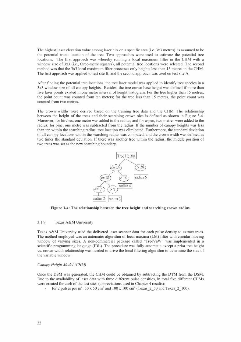
The crown widths were derived based on the training tree data and the CHM. The relationship between the height of the trees and their searching crown size is defined as shown in Figure 3-4. Moreover, for birches, one metre was added to the radius; and for aspen, two metres were added to the radius; for pine, one metre was subtracted from the radius. If the number of canopy heights was less than ten within the searching radius, tree location was eliminated. Furthermore, the standard deviation of all canopy locations within the searching radius was computed, and the crown width was defined as two times the standard deviation. If there was another tree within the radius, the middle position of two trees was set as the new searching boundary.

Figure 3-4: The relationship between the tree height and searching crown radius.

3.1.9 Texas A&M University

Texas A&M University used the delivered laser scanner data for each pulse density to extract trees. The method employed was an automatic algorithm of local maxima (LM) filter with circular moving window of varying sizes. A non-commercial package called “TreeVaW” was implemented in a scientific programming language (IDL). The procedure was fully automatic except a prior tree height vs. crown width relationship was needed to drive the local filtering algorithm to determine the size of the variable window.

Canopy Height Model (CHM)

Once the DSM was generated, the CHM could be obtained by subtracting the DTM from the DSM. Due to the availability of laser data with three different pulse densities, in total five different CHMs were created for each of the test sites (abbreviations used in Chapter 4 results):

- for 2 pulses per m2: 50 x 50 cm2 and 100 x 100 cm2 (Texas_2_50 and Texas_2_100).

23

- for 4 pulses per m2: 50 x 50 cm2 (Texas_4_50). - for 8 pulses per m2: 25 x 25 cm2 and 50 x 50 cm2 (Texas 8_25 and Texas 8_50).

Locating Individual Trees by Local Filtering with a Variable Window Size

Local Maximum Filter is often used to locate tree position based on the assumption that the highest elevation corresponds to the tree apex. When applying the LM filter, the window size has great influences on tree identification. If the window size is too small or too large, commission or omission errors most likely occur. Furthermore, a fixed window size is inconsistent with the complex canopy structure of hardwoods and mixed pine-hardwoods. It will be more flexible and robust to employ a variable window of circular shape whose size is adjusted adaptively according to the spatial neighbourhood (Figure 3-5).

Figure 3-5: A Circular Window (white area) inscribed to a square window (19 X 19 pixels).

On the other hand, the taller the tree is, the larger the crown width. Thus the determination of filter size was based on the relationship between the crown size and tree height. Prior information can be utilized to derive such a relationship; to predict the crown size, regression models are fitted with tree height as the independent variable.

For the Espoonlahti data, about ninety trees for each test site were visually identified from the CHMs and the corresponding heights and crown width were manually recorded by on-screen measurement. The trees obtained were used to develop linear models for the relationship between tree height and crown width. The resulting equations are shown below for Site A and Site B respectively.

- Crown Width = 1.29 + 0.27 * Tree Height (Site A) - Crown Width = 1.66 + 0.23 * Tree Height (Site B)

The Calculation of Crown Width

Based on the tree locations identified by the above LM filtering, crown width could be further estimated from the CHM. First, a 3x3 median filter was applied to the original CHM to suppress possible noise in the highly complex surface. The median filter was preferred since it does not affect original values in the CHM, plus it is an edge preserving filter, better suited for conserving the delineation between adjacent tree crowns.

The crown diameter is the average of two values measured along two perpendicular directions from the location of the tree top. To describe the crown profiles along the two directions on the CHM, the algorithm fits a fourth-degree polynomial to both profiles. The length of each of the two profiles is limited to twice the window size and is centred on the tree top. The fourth-degree polynomial allows the corresponding function to have a concave shape along the crown profile of a single tree, with three

24

extreme values. The fitted function closely follows the vertical profile of a tree crown (Figure 3-6) and its graph has a maximum in the neighbourhood of the tree top, where the first derivative equals 0 and the second derivative is negative. Points of inflection occur on the edges of a crown profile. When these conditions are met, i.e., the fitted function indicates a tree crown profile, the distance between critical points is used to calculate the crown diameter. The final value for a crown diameter is computed as the average of the crown diameters measured in the two perpendicular directions or profiles. Figure 3-7 lists the flowchart of the algorithm for measuring crown width.

Due to the complexity of the CHM, sometimes the first and second derivatives cannot provide real solutions and crown diameter cannot be measured. This method seems appropriate to measure crown diameter for dominant and co-dominant trees that have individualized crowns on the CHM surface.

25

Figure 3-6: Vertical profiles through the CHM and the fitted polynomials for a deciduous tree and a pine located in the centre of the CHM “image” (a) and (b), respectively; (c) and (d) show vertical profiles along the horizontal direction for the deciduous and the pine trees; (e) and (f)

are vertical profiles along the vertical direction (deciduous and pine trees, respectively).

26

Figure 3-7: Flow chart of algorithm for measuring crown width.

Estimating the Height to Crown Base

In most cases, the upper laser hits, used for DSM, and the lower hits, for DTM only, cover a small portion of the full dataset. A relatively large percent of laser hits may not be involved in the processing of the above algorithms. Intuitively, the full set of laser hits should provide a more detailed characterization of canopy surface than only the upper and lower subsets; specifically more information on tree structure along the vertical dimension is expected to be revealed by doing so. The vertical profile provides some hints on the height to crown base.

3.1.10 University of Zürich

The approach used by the University of Zürich is quite similar to the one described in Morsdorf et al. (2004). It is based on local maxima detection in the CHM and a following cluster analysis of the raw data with found local maxima as starting points. Some changes in the local maxima derivation part were undertaken, which will be described in further detail below.

27

Digital Surface Model (DSM)

Since the data was delivered in raw form and only the DTM was provided, Zürich generated the DSM using a routine developed in-house. The DSM generation includes the choice of four parameters, which are destination grid resolution, search radius, and size and shape of a Gaussian smoothing function. In sensitivity studies the latter was found to have only a small influence on the form of the DSM and thus a fixed value was used. The first three parameters were used as free variables when optimizing the local maxima filter using the reference data.

Local Maxima

Figure 3-8: Graphic User Interface (GUI) for tuning the relevant parameters of DSM generation and local maxima detection. Left panel shows DSM without smoothing, the right one the DSM after the morphological opening operation. White dots denote found local maxima, whereas black dots are reference tree positions.

The local maxima detection algorithm was changed from the one used in Morsdorf et al. (2004). Since the generation of the DSM already comprised one instance of smoothing (Gaussian weights on raw data inside the search radius), a morphological opening operation was done to further improve the detection of local maxima. The opening operation (a dilation followed by an erosion) was done using a (presumably) crown shaped structuring element of varying size. In order not to have too many free parameters for filter tuning, this size was set to the size of the Gaussian smoothing kernel used for DSM generation. A small MATLAB GUI was constructed for selection of appropriate values for these parameters based on the reference data (tree positions). The GUI is depicted in Figure 3-8, with sliders and edit boxes for all four parameters. As mentioned above, the shape of the Gaussian smoothing kernel had little effect and thus a constant value of 0.7 was used (right edit box).

28

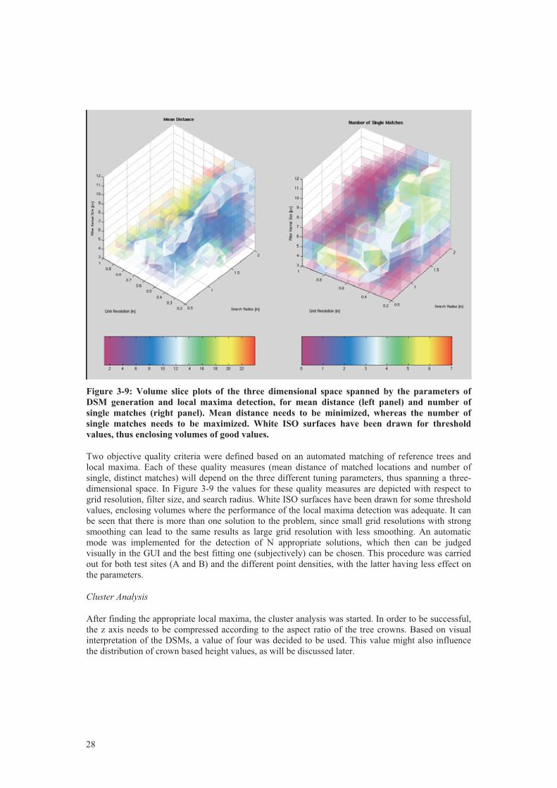
Figure 3-9: Volume slice plots of the three dimensional space spanned by the parameters of DSM generation and local maxima detection, for mean distance (left panel) and number of single matches (right panel). Mean distance needs to be minimized, whereas the number of single matches needs to be maximized. White ISO surfaces have been drawn for threshold values, thus enclosing volumes of good values.

Two objective quality criteria were defined based on an automated matching of reference trees and local maxima. Each of these quality measures (mean distance of matched locations and number of single, distinct matches) will depend on the three different tuning parameters, thus spanning a three-dimensional space. In Figure 3-9 the values for these quality measures are depicted with respect to grid resolution, filter size, and search radius. White ISO surfaces have been drawn for some threshold values, enclosing volumes where the performance of the local maxima detection was adequate. It can be seen that there is more than one solution to the problem, since small grid resolutions with strong smoothing can lead to the same results as large grid resolution with less smoothing. An automatic mode was implemented for the detection of N appropriate solutions, which then can be judged visually in the GUI and the best fitting one (subjectively) can be chosen. This procedure was carried out for both test sites (A and B) and the different point densities, with the latter having less effect on the parameters.

Cluster Analysis

After finding the appropriate local maxima, the cluster analysis was started. In order to be successful, the z axis needs to be compressed according to the aspect ratio of the tree crowns. Based on visual interpretation of the DSMs, a value of four was decided to be used. This value might also influence the distribution of crown based height values, as will be discussed later.

29

Based on the reference data, the settings had to be chosen using the GUI and the auto mode suggestions. Except for the setting of these parameters, the approach is fully automated and does not need any user intervention.

The outcome of the cluster analysis is the raw data being flagged with a distinct number of all returns presumably belonging to a tree. This cluster is then treated by a routine which takes the relevant measures from the point cloud. These are the following:

- Position (x, y) is derived as the centre of gravity of the echo positions belonging to the cluster.

- Tree height is computed as the maximum height of the cluster’s echos. - Crown diameter is estimated using the convex hull of the cluster by transferring the

circumdistance of the convex hull to a radius assuming circular shape. - Crown base height is computed as the minimum of the cluster’s echos. - Crown outline is the two-dimensional convex hull of the cluster’s points projected into the x,

y-plane. The histograms of the output values can be used to check whether there are outliers as very high trees (e.g. caused by erroneous laser returns (bird echoes)) or extremely large crowns (e.g. buildings). For example it could be seen that there are a lot of crown base heights (CBH) with the value of zero. The tuning of the scaling parameter for the z axis could help improve the CBH value distribution.

3.1.11 Progea Consulting and Agricultural University of Cracow

Progea Consulting and Agricultural University of Cracow used aerial images and a beta version of a self developed protocol, tree counting robot, in eCognition software to count the amount of trees within a single image. Tree counting robot does not need training data. The main aim was to find the centre of a single tree.

3.1.12 University of Udine

The experiments were performed using an original software developed within the Department of Geo-resources and Territory of the University of Udine.

The main components of the software allow visualisation of the laser scanning data, section drawings, DTM and DSM calculation and their overlap with other cartographic maps.

On this basis a specific tool was implemented in order to extract some interesting forestry parameters such as:

- Position and counting of the single tree. - Tree height calculation. - Crown delineation. - Crown depth calculation. - Crown volume calculation.

The extracted data was subsequently organized and managed in a Geographic Information System (GIS). The method was applied in a completely automatic way. In particular, the same input parameters were used to process all the dataset. However, some parameters can be manually optimized if a detailed forest typology and its ecological structure are known.

The implemented method was exclusively based on laser scanning data. The procedure constituted a sequence of elaborations and transformations upon raw data and was schematically based on the following two methodological approaches:

30

1. Application of morphological algorithms for the location of the trees. 2. Location of the laser points belonging to the single crown through a clustering algorithm.

The work scheme and the implemented algorithms will be subsequently specified.

Tree location

Ground point filtering is a necessary procedure for the calculation of tree height. This operation was carried out using the Axelsson algorithm, implemented in Udine’s experimental software. Moreover an algorithm which removes the points (ground and not ground) derived from the echoes penetrated inside the crown from the dataset, was implemented. At first, the algorithm provides a triangulation of all the points; the following step is the removal of all the vertexes that present a difference greater than a fixed threshold. The procedure therefore allows a correct DSM to be obtained.

The method applied for tree counting is based on a morphological analysis of the laser point distribution. For this purpose the Top Hat algorithm was implemented. This is a mathematical function of image elaboration which allows the top elements at the scale of the represented values to be found. The mathematical formulation of the Top Hat is related to the theory of image processing formulated by Serra (1982, 1988).

The result of the image transformation is an image without levels of local background. Considering f(x) as the grey value of a generic pixel x of a point localized in u, and f(X) as the corresponding value of the transformation of the entire matrix X, � is defined as the structural geometric element to determine or as the dimension of the explorative matrix (kernel) centred in x.

Therefore the following transformations of Erosion and Dilatation (Rodriguez et al., 2002) as well as Opening is defined as follows:

- Erosion: E� f(X) = inf { f(u) : u � �x } - Dilatation: D� f(X) = sup { f(u) : u � �x } - Opening: O� f(X) = D� (E� f(X))

The Top Hat function is based on the Opening function and is used to identify the local maxima in the scale of the image values. The extraction of such elements is carried out by using the function Top that operates a difference between the primitive image (function) and the Opening transformed:

- TOP: { x : f(x) - O� f(X)} Only the elements of the image that have bigger dimensions than the structural element � are maintained.

Enlarging the concept of Top Hat directly to the laser data, the Udine approach allows detection of the set of points belonging to the top of the crown directly from the point cloud of the “correct” DSM. The application of a subsequent rank filter allows detection of the local maximum starting from the points classified as “top”. It is therefore possible to obtain the position in space (x,y,z) of the apex points directly on the laser (classification) data. The coordinates x,y of these points are assumed to correspond to the positions of the single trees.

In some cases, because of the presence of small height variations among adjoining points belonging to the same crown, more than one apex can be counted for each tree. In order to minimize this kind of error a control algorithm was introduced. It detects and corrects the apexes which are erroneously classified (these are often localized at the edge of the crown). The algorithm analyzes the height of each apex in comparison to the close laser points, using an opportune search radius. If a point with a higher altitude within the research window exists, this same point becomes the new apex. The procedure runs iteratively until the convergence between the intermediate apexes and the nearest correct apex is obtained.

31

The tree height is calculated as the difference between the z value of the apexes and the height of the corresponding ground. According to the definition of wood suggested by the “Italian National Forest and Carbon Inventory” it is possible to exclude from the count those trees which present a lower height than a given threshold. In this work apexes with an altitude lower than two metre on the ground have not been considered as a “tree”.

Crown delineation

In order to delineate single crowns an algorithm of region growing was implemented. Beginning from the apexes previously identified, the algorithm clusters the vegetation points on the basis of the following principles:

- If the points located in the proximity of the apex are lower (height difference) than a fixed threshold, these are marked as belonging to the same cluster.

- For each marked point the same procedure is iteratively applied. It may happen that the same laser point is marked as belonging to different apexes; this is particularly true when the forest is characterized by close vegetation. In this case the algorithm associates the point to the nearest apex.

The crowns were delineated using polygon circles of which the parameters (centre and radius) are calculated analysing the planimetric coordinates of the points belonging to the clusters. The geometric barycentre of the point distribution is assumed as the centre of the crown (in most cases the centre of the circle does not correspond to the coordinates of the respective apex). Each circle polygon is drawn using a radius equal to the equation:

radius = [(x Max – x min) + (y Max – y min)] /4

Height of crown base

The crown depth was calculated as the difference between the maximum height and the minimum height of the points belonging to the cluster. Moreover, the height of crown insertion was calculated in terms of difference between the tree height and the crown depth.

The crown volume is calculated using the following equation: Crown_volume = CHM – [Crown area x (tree_height – crown_depth)]

where the CHM is derived by subtracting the height value of the DTM at each pixel from the height value of the DSM.

3.2 Methods for Accuracy Evaluation of Participants’ Tree Models

Tree location accuracy was evaluated by measuring distances from every reference tree to the nearest tree found on the delivered model. For tree location the coordinates of the reference tree top were used. Only distances within five metres from the reference tree were included in the analysis. If several reference trees had hits on the same tree in the analyzed model, only the best match according to distance and height was accepted for analysis purposes, other observations were disregarded. Location accuracy was analyzed for two cases: all trees and trees over 15 m tall.

The trees approved for location accuracy evaluation (as described above) were also used for tree height evaluation, and again two cases were used: all trees and trees over 15 m tall. Again, the trees approved for location accuracy evaluation were also used for crown base height evaluation and tree species classification accuracy evaluation. In tree species classification only three classes were used: pine, spruce and deciduous.

32

The crown delineation accuracy was evaluated by comparing the total delineated area of reference trees on test plots to the area obtained from delivered model delineation (total relative crown area difference). If a participant did not deliver crown delineation as vector data, the crown covered area was determined as a circle around the trunk location by using the given radius or area, and final delineated area was obtained as a union of these circles. Also total relative shape dissimilarity (Henricsson & Baltsavias, 1997) was computed. Total relative shape dissimilarity is the sum of the area difference and the remaining overlap error, i.e. the sum of missing area and extra area divided by the reference area.

In order to get an idea of what accuracy of tree extraction can be achieved manually using the same data, trees in the reference test plots were manually extracted by a FGI employee. Extraction was executed using laser scanner data (8 points per m2) and GIS software. Aerial images were used only for interpretation purposes. Trees were delineated visually by using laser points which were colour coded based on the elevation, and the location and height were measured by finding the highest laser points within the delineated trees. Ground height was interpreted visually in 3D-view. The results of this manual extraction are marked as “Manual” in the figures and tables in Chapter 4, Results.

If the observed value differed from the reference value by more than 3*std ± mean observation, it was considered as a gross error, i.e. outlier, and removed. In the tree height analysis, at first all values deviating by more than 10 metres from the ground truth were removed.

Root mean squared error (abbreviated to RMSE, Equation 3-1) was calculated for tree location, height and crown base height after gross errors were removed.

� �

n

eeRMSE

n

iii�

�

�� 1

221

(Equation 3-1)

where e1i is the result obtained with the described retrieved model, e2i is the corresponding reference measured value, and n is the number of samples. Additionally, minimum, maximum, medium, mean and standard deviation values were calculated.

Descriptive statistics are presented before and after outliers have been removed. In figures and tables laser point densities are marked after the participant name, for example, FOI_2 for two points, FOI_4 for four points and FOI_8 for eight points per m2.

3.3 Examples of Extracted Models

Examples of extracted tree models are shown in Figures Figure 3-10 and Fehler! Verweisquelle konnte nicht gefunden werden.. The Figures nicely indicate that some methods tend mainly to extract tree groups or larger dominant trees, and some of them can separate individual trees of the dominant and co-dominant layers. Suppressed trees are mainly neglected. Norwegian models also find more smaller trees but also creates tree positions in places, where there are no real trees.

33

Figu

re 3

-10:

Exa

mpl

es o

f ext

ract

ed m

odel

s. G

reen

dot

s are

ref

eren

ce tr

ees,

size

dep

ende

nt o

n tr

ee h

eigh

t. R

ed d

ots a

re e

xtra

cted

tree

s, fo

r so

me

part

icip

ants

als

o th

e cr

own

delin

eatio

n is

show

n.

34

Figu

re 3

-11:

Exa

mpl

es o

f ext

ract

ed m

odel

s. G

reen

dot

s are

ref

eren

ce tr

ees,

size

dep

ende

nt o

n tr

ee h

eigh

t. R

ed d

ots a

re e

xtra

cted

tree

s, fo

r so

me

part

icip

ants

als

o th

e cr

own

delin

eatio

n is

show

n. C

anad

a =

Paci

fic F

ores

try

Cen

tre.

35

4 Results

4.1 Amount of Extracted Trees

The amount of extracted trees on the reference test plots is shown in Figure 4-1. The amount of extracted trees reveals how many percent of the true trees have been extracted. In order to provide non-biased estimates e.g. for volume, the correct percentage rate should be as high as possible. Obviously, there were significant differences between the models. Udine and Norwegian models provided the highest sensitivity for smaller trees, where as Progea, Definiens, Hannover and Texas models mainly presented the dominating trees or some of them.

0.010.020.030.040.050.060.070.080.090.0

100.0

Prog

eaD

efin

iens

FOI_

2FO

I _4

FOI_

8PF

C_a

eria

lPF

C_l

aser

Han

nove

r_2

Han

nove

r _4

Han

nove

r_8

Joan

neum

_aer

ial

Joan

neum

_hyb

ridM

etla

_2M

etla

_4M

etla

_8N

orw

a y_2

Nor

way

_4N

orw

ay_8

Ilian

_2Ili

an_4

Ilian

_8Te

xas_

2_10

0Te

xas_

2_50

Texa

s _4_

50Te

xas_

8_50

Texa

s _8_

25U

dine

_2U

dine

_4U

dine

_8Zu

rich_

2Zu

rich _

4Zu

rich_

8M

anua

l

[%]

Amount of Extracted Trees

Figure 4-1: The amount of extracted trees on reference test plots as a percentage of the total number of reference trees.

36

4.2 Tree Location Accuracy

Tree location accuracy is shown separately for all trees (Figure 4-2, Table 4-1) and trees over 15 m tall (Figure 4-3, Table 4-2).

0.0

0.5

1.0

1.5

2.0

Prog

eaD

efin

iens

FOI_

2FO

I_4

FOI_

8PF

C_a

eria

lPF

C_l

aser

Han

nove

r_2

Han

nove

r_4

Han

nove

r_8

Joan

neum

_aer

ial

Joan

neum

_hyb

…M

etla

_2M

etla

_4M

etla

_8N

orw

ay_2

Nor

way

_4N

orw

ay_8

Ilian

_2Ili

an_4

Ilian

_8Te

xas_

2_10

0Te

xas_

2_50

Texa

s_4_

50Te

xas_

8_50

Texa

s_8_

25U

dine

_2U

dine

_4U

dine

_8Zu

rich_

2Zu

rich_

4Zu

rich_

8M

anua

l

[m]

Tree Location, all trees (outliers removed)MeanSTDRMSE

Figure 4-2: Tree location accuracy, all trees.

0.0

0.5

1.0

1.5

2.0

Prog

eaD

efin

iens

FOI_

2FO

I_4

FOI _

8PF

C_a

eria

lPF

C_l

aser

Han

nove

r_2

Han

nove

r _4

Han

nove

r_8

Joan

neum

_aer

ial

Joan

neum

_hyb

…M

etla

_2M

etla

_4M

etla

_8N

orw

ay_2

Nor

wa y

_4N

orw

a y_8

Ilian

_2Ili

an_4

Ilian

_8Te

xas _

2_10

0Te

xas _

2_50

Texa

s_4_

50Te

xas_

8_50

Texa

s _8_

25U

dine

_2U

dine

_4U

dine

_8Zu

rich_

2Zu

rich _

4Zu

rich_

8M

anua

l

[m]

Tree Location, trees over 15 m tall (outliers removed)MeanSTDRMSE

Figure 4-3: Tree location accuracy, trees over 15 m tall.

All

obse

rvat

ions

Progea

Definiens

FOI_2

FOI_4

FOI_8

PFC_aerial

PFC_laser

Hannover_2

Hannover_4

Hannover_8

Joanneum_aerial

Joanneum_hybrid

Metla_2

Metla_4

Metla_8

Norway_2

Norway_4

Norway_8

Ilian_2

Ilian_4

Ilian_8

Texas_2_100

Texas_2_50

Texas_4_50

Texas_8_50

Texas_8_25

Udine_2

Udine_4

Udine_8

Zurich_2

Zurich_4

Zurich_8

Manual

Mea

n 1.

41 1

.64

0.74

0.6

7 0.

63 1

.41

1.39

1.32

1.21

1.15

1.59

0.90

0.80

0.74

0.70

0.73

0.77

0.75

0.7

9 0.

820.

791.

010.

860.

840.

860.

770.

800.

760.

731.

111.

071.24

0.64

Med

ian

1.27

1.1

3 0.

57 0

.53

0.42

1.22

1.14

1.12

1.00

0.92

1.48

0.65

0.57

0.46

0.45

0.50

0.52

0.43

0.6

0 0.

540.

500.

700.

660.

690.

670.

480.

570.

530.

460.

940.

901.

060.

39ST

D

0.77

1.2

8 0.

67 0

.63

0.66

0.8

90.

990.

990.

820.

800.

840.

830.

730.

740.

700.

690.

710.

78 0

.66

0.79

0.76

0.87

0.68

0.66

0.73

0.79

0.68

0.68

0.71

0.72

0.72

0.76

0.70

Min

0.

13 0

.02

0.09

0.0

5 0.

02 0

.09

0.01

0.06

0.03

0.09

0.19

0.03

0.05

0.05

0.05

0.02

0.01

0.03

0.0

1 0.

010.

010.

080.

080.

100.

050.

070.

010.

010.

010.

100.

070.

090.

01M

ax

4.59

4.6

8 4.

45 3

.73

3.46

4.3

74.

544.

824.23

4.38

4.96

4.44

3.99

3.94

3.97

3.47

3.62

3.47

3.7

9 3.

903.

494.

093.

393.

594.25

4.59

3.89

3.90

3.65

3.23

3.73

4.28

4.07

Num

ber

154

121

184

185 20

6 17

317

510

910

310

1202

19921220

920

322

824223

9 22

4 21

820

912

114

6142

135

13323

923

823

021220

520

721

1O

utlie

rsre

mov

ed

Mea

n 1.

33 1

.64

0.66

0.6

0 0.

53 1

.40

1.36

1.23

1.15

1.12

1.56

0.83

0.72

0.68

0.64

0.66

0.73

0.67

0.72

0.77

0.74

0.96

0.79

0.76

0.78

0.72

0.74

0.71

0.68

1.11

1.06

1.21

0.57

Med

ian

1.21

1.1

3 0.

55 0

.52

0.40

1.22

1.14

1.11

1.00

0.91

1.48

0.64

0.55

0.45

0.44

0.48

0.51

0.42

0.5

8 0.

530.

490.

700.

650.

690.

660.

480.

560.

520.

450.

940.

901.

040.

38ST

D

0.61

1.2

8 0.

48 0

.46

0.45

0.8

60.

940.

840.

710.

740.

780.

700.

590.

610.

590.

550.

640.

66 0

.53

0.71

0.68

0.78

0.56

0.51

0.55

0.68

0.58

0.57

0.60

0.72

0.69

0.71

0.52

Min

0.

13 0

.02

0.09

0.0

5 0.

02 0

.09

0.01

0.06

0.03

0.09

0.19

0.03

0.05

0.05

0.05

0.02

0.01

0.03

0.0

1 0.

010.

010.

080.

080.

100.

050.

070.

010.

010.

010.

100.

070.

090.

01M

ax

3.32

4.6

8 2.

49 2

.53 2.

59 3

.66

3.89

4.22

3.66

3.37

4.10

3.312.

922.

942.

662.

642.

753.

06 2

.53

3.162.

963.

582.

762.

762.

903.

102.

612.

672.

833.23

3.05

3.342.

57N

umbe

r 15

012

1 17

8 18

0 19

8 172

173

106

101

10020

019

520

620

419

922

123

8232 21

8 21

420

511

9142

138

131

13123

423

322

521220

420

520

6R

MSE

1.

46 2

.07

0.81

0.7

6 0.

70 1

.64

1.65

1.48

1.35

1.34

1.75

1.08

0.93

0.91

0.87

0.86

0.97

0.94

0.8

9 1.

051.

011.24

0.97

0.92

0.95

0.99

0.94

0.91

0.91

1.33

1.27

1.40

0.77

Tab

le 4

-1: T

ree

loca

tion

accu

racy

in m

etre

s, al

l tre

es.

37

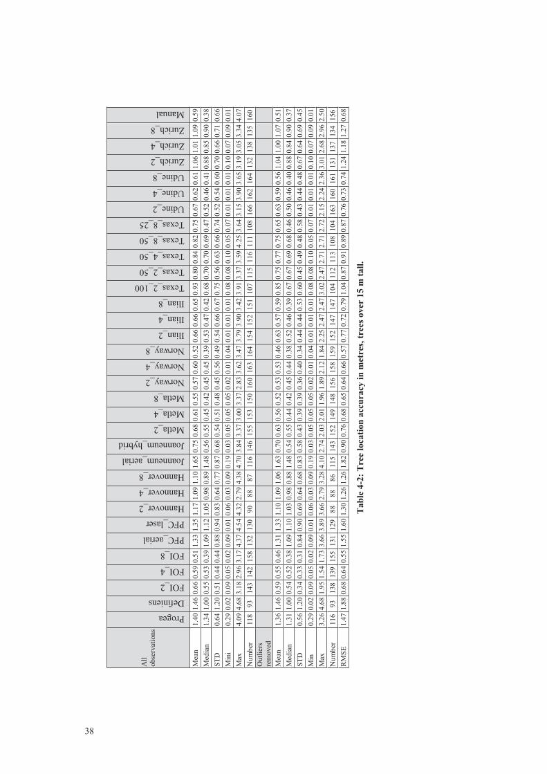
All

obse

rvat

ions

Progea

Definiens

FOI_2

FOI_4

FOI_8

PFC_aerial

PFC_laser

Hannover_2

Hannover_4

Hannover_8

Joanneum_aerial

Joanneum_hybrid

Metla_2

Metla_4

Metla_8

Norway_2

Norway_4

Norway_8

Ilian_2

Ilian_4

Ilian_8

Texas_2_100

Texas_2_50

Texas_4_50

Texas_8_50

Texas_8_25

Udine_2

Udine_4

Udine_8

Zurich_2

Zurich_4

Zurich_8

Manual

Mea

n 1.

40 1

.46

0.66

0.5

9 0.

51 1

.33

1.35

1.17

1.09

1.10

1.65

0.75

0.68

0.61

0.55

0.57

0.60

0.52

0.6

6 0.

660.

650.

930.

800.

840.

820.

750.

670.

620.

611.

061.

011.

090.

59M

edia

n 1.

34 1

.00

0.55

0.5

3 0.

39 1

.09

1.12

1.05

0.98

0.89

1.48

0.56

0.55

0.45

0.42

0.45

0.45

0.39

0.5

3 0.

470.

420.

680.

700.

700.

690.

470.

520.

460.

410.

880.

850.

900.

38ST

D

0.64

1.2

0 0.

51 0

.44

0.44

0.8

80.

940.

830.

640.

770.

870.

680.

540.

510.

480.

450.

560.

49 0

.54

0.66

0.67

0.75

0.56

0.63

0.66

0.74

0.52

0.54

0.60

0.70

0.66

0.71

0.66

Min

i 0.29

0.02

0.09

0.0

5 0.

02 0

.09

0.01

0.06

0.03

0.09

0.19

0.03

0.05

0.05

0.05

0.02

0.01

0.04

0.0

1 0.

010.

010.

080.

080.

100.

050.

070.

010.

010.

010.

100.

070.

090.

01M

ax

4.09

4.6

8 3.

18 2

.96

3.17

4.3

74.

544.

322.

794.

384.

703.

843.

373.

003.

372.

833.

623.

47 3

.79

3.90

3.42

3.91

3.37

3.59

4.25

3.64

3.15

3.90

3.65

3.19

3.05

3.34

4.07

Num

ber

118

93

143

142

158

132

130

90

88

87

116

146

155

153

150

160

163

164

154

152

151

107

115

116

111

108

166

162

164

132

138

135

160

Outlie

rsre

mov

ed

Mea

n 1.

36 1

.46

0.59

0.5

5 0.

46 1

.31

1.33

1.10

1.09

1.06

1.63

0.70

0.63

0.56

0.52

0.53

0.53

0.46

0.6

3 0.

570.

590.

850.

750.

770.

750.

650.

630.

590.

561.

041.

001.

070.

51M

edia

n 1.

31 1

.00

0.54

0.52

0.38

1.0

91.

101.

030.

980.

881.

480.

540.

550.

440.

420.

450.

440.

38 0

.52

0.46

0.39

0.67

0.67

0.69

0.68

0.46

0.50

0.46

0.40

0.88

0.84

0.90

0.37

STD

0.

56 1

.20

0.34

0.3

3 0.

31 0

.84

0.90

0.69

0.64

0.68

0.83

0.58

0.43

0.39

0.39

0.36

0.40

0.34

0.4

4 0.

440.

530.

600.

450.

490.

480.

580.

430.

440.

480.

670.

640.

690.

45M

in

0.29

0.02

0.09

0.0

5 0.

02 0

.09

0.01

0.06

0.03

0.09

0.19

0.03

0.05

0.05

0.05

0.02

0.01

0.04

0.0

1 0.

010.

010.

080.

080.

100.

050.

070.

010.

010.

010.

100.

070.

090.

01M

ax

3.26

4.6

8 1.

95 1

.54

1.73

3.6

63.

893.

662.

793.28

4.102.

742.

032.

011.

961.

892.

121.

84 2

.25 2.

472.

473.

022.

472.

712.

712.

722.

152.242.

363.

012.

682.

962.

50N

umbe

r 11

693

13

8 13

9 15

5 13

112

988

88

86

11

514

3152

149

148

156

158

159

152

147

147

104

112

113

108

104

163

160

161

131

137

134

156

RMSE

1.

47 1

.88

0.68

0.6

4 0.

55 1

.55

1.60

1.30

1.26

1.26

1.82

0.90

0.76

0.68

0.65

0.64

0.66

0.57

0.7

7 0.

720.

791.

040.

870.

910.

890.

870.

760.

730.

741.24

1.18

1.27

0.68

Tab

le 4

-2: T

ree

loca

tion

accu

racy

in m

etre

s, tr

ees o

ver

15 m

tall.

38

39

4.3 Tree Height Accuracy

There are big differences in tree height determination accuracy between different methods (Figure 4-4, Figure 4-5, Table 4-3 and Table 4-4). For Ilian method the accuracy is greatly improved when only taller trees are considered, as is the case also for Pacific Forestry Centre and Joanneum’s hybrid methods. For most methods the tree height is underestimated, as was expected, but overestimated for Hannover and, when all trees are considered, for Zürich. Manual extraction is less accurate than best automatic methods, which are not forced to follow the actual laser points thus resulting in better representation of true tops of the trees.

-2.0

-1.0

0.0

1.0

2.0

3.0

4.0

5.0

Def

inie

nsFO

I_2

FOI_

4FO

I_8

PFC

_aer

ial

PFC

_las

erH

anno

ver_

2H

anno

ver_

4H

anno

ver_

8Jo

anne

um_h

ybrid

Met

la_2

Met

la_4

Met

la_8

Nor

way

_2N

orw

ay_4

Nor

way

_8Ili

an_2

Ilian

_4Ili

an_8

Texa

s_2_

100

Texa

s_2_

50Te

xas_

4_50

Texa

s_8_

50Te

xas_

8_25

Udi

ne_2

Udi

ne_4

Udi

ne_8

Zuric

h_2

Zuric

h_4

Zuric

h_8

Man

ual

[m]

Tree Height, all trees (outliers removed)

MeanSTDRMSE

Figure 4-4: Tree height accuracy, all trees.

-2.0

-1.0

0.0

1.0

2.0

3.0

4.0

5.0

Def

inie

nsFO

I_2

FOI_

4FO

I_8

PFC

_aer

ial

PFC

_las

erH

anno

ver_

2H

anno

ver_

4H

anno

ver_

8Jo

anne

um_h

ybrid

Met

la_2

Met

la_4

Met

la_8

Nor

way

_2N

orw

ay_4

Nor

way

_8Ili

an_2

Ilian

_4Ili

an_8

Texa

s_2_

100

Texa

s_2_

50Te

xas_

4_50

Texa

s_8_

50Te

xas_

8_25

Udi

ne_2

Udi

ne_4

Udi

ne_8

Zuric

h_2

Zuric

h_4

Zuric

h_8

Man

ual

[m]

Tree Height, trees over 15 m (outliers removed)

MeanSTDRMSE

Figure 4-5: Tree height accuracy, trees over 15 m.

All

obse

rvat

ions

Definiens

FOI_2

FOI_4

FOI_8

PFC_aerial

PFC_laser

Hannover_2

Hannover_4

Hannover_8

Joanneum_hybrid

Metla_2

Metla_4

Metla_8

Norway_2

Norway_4

Norway_8

Ilian_2

Ilian_4

Ilian_8

Texas_2_100

Texas_2_50

Texas_4_50

Texas_8_50

Texas_8_25

Udine_2

Udine_4

Udine_8

Zurich_2

Zurich_4

Zurich_8

Manual

Mea

n -1

.53

-0.0

9 -0

.40

-0.0

8 0.

33-0

.03

1.40

3.71

3.88

0.38

-0.3

7-0

.25

0.13

0.59

0.93

0.73

-0.02

0.43

0.

36-0

.74

-0.9

4-0

.71

-0.4

3-0

.38

0.14

0.33

0.66

0.36

0.98

1.01

0.25

Med

ian

-1.4

7 -0

.60

-0.5

0 -0

.30

-0.6

0-0

.49

1.35

4.65

4.33

-0.3

3-0

.55

-0.4

7-0

.25

0.20

0.16

0.01

-0.6

5 -0

.45

-0.3

0-1

.22

-0.9

7-0

.86

-0.6

3-0

.50

-0.5

8-0

.43

-0.2

6-0

.44

0.03

0.12

-0.4

6

STD

2.26

2.

05

0.98

1.

68 2.

672.

931.

442.

692.

662.

401.

351.

531.

861.

752.

512.

382.

67 2.

66 2.

622.29

0.61

1.61

1.37

0.96

2.62

2.62

2.66

3.29

2.82

2.88

2.42

Min

-7

.57

-2.2

4 -1

.67

-2.8

4 -3

.08

-8.02

-0.9

5-0

.77

-0.7

7-3

.09

-4.0

5-2

.02

-1.4

7-2

.47

-1.5

0-2

.12

-7.1

3 -3

.70

-8.5

8-2

.79

-3.1

5-5

.80

-1.9

9-1

.28

-3.3

7-3

.29

-2.2

6-9

.62

-4.4

6-5

.82

-2.9

1

Max

7.

45

9.25

7.

95

9.25

9.

679.

039.

047.

998.

789.

956.

979.

969.

969.

329.

809.

799.

87

9.97

9.

979.

630.

569.

769.

646.

629.

969.

559.

819.

959.

559.

149.

92

Num

ber

67

104

104

115

100

97

58

55

55

109

121

120

119

122

134

132

130

129

125

63

82

84

77

78

135

131

130

132

119

128

123

Outlie

rsre

mov

ed

Mea

n -1

.67

-0.3

4 -0

.48

-0.3

8 0.23

-0.2

11.26

3.71

3.88

0.06

-0.5

8-0

.47

-0.2

30.

340.

460.27

-0.32

0.15

0.27

-1.2

0-0

.92

-0.8

6-0

.56

-0.4

7-0

.35

0.05

0.31

0.44

0.91

1.01

-0.1

9

Med

ian

-1.4

9 -0

.61

-0.5

0 -0

.32

-0.6

0-0

.53

1.34

4.65

4.33

-0.3

5-0

.56

-0.4

9-0

.27

0.17

0.14

-0.0

3-0

.68

-0.4

7 -0

.30

-1.3

1-0

.97

-0.8

6-0

.64

-0.5

1-0

.64

-0.4

6-0

.27

-0.4

00.

010.

12-0

.48

STD

1.

99

1.47

0.

53

0.53

2.

512.

651.

022.

692.

661.

780.

720.

590.

741.

071.

551.

412.

12 2.

18 2.21

0.96

0.56

0.57

0.73

0.52

1.64

2.14

2.03

3.19

2.72

2.88

1.45

Min

-7

.57

-2.2

4 -1

.67

-2.8

4 -3

.08

-8.02

-0.9

5-0

.77

-0.7

7-3

.09

-4.0

5-2

.02

-1.4

7-2

.47

-1.5

0-2

.12

-7.1

3 -3

.70

-3.9

8-2

.79

-2.4

1-2

.81

-1.9

9-1

.28

-3.3

7-3

.29

-2.2

6-8

.65

-4.4

6-5

.82

-2.9

1

Max

3.

37

5.91

2.

03

0.66

8.

107.

744.

097.

998.

786.

943.

122.

694.

335.

657.

507.

667.

65

7.99

8.

343.

140.

560.

183.

132.

057.

058.

168.

179.

959.

339.

146.29

Num

ber

66

101

103

111

99

95

57

55

55

105

117

117

114

118

127

125

126

125

122

60

81

81

76

77

128

127

125

131

118

128

117

RMSE

2.58

1.

50

0.71

0.

65 2.

512.

651.

624.

564.

691.

770.

930.

760.

771.

121.

611.

432.

13 2.

17 2.22

1.53

1.07

1.03

0.92

0.70

1.67

2.13

2.05

3.21

2.86

3.04

1.45

Tab

le 4

-3: T

ree

heig

ht a

ccur

acy

in m

etre

s, al

l tre

es.

40

All

obse

rvat

ions

Definiens

FOI_2

FOI_4

FOI_8

PFC_aerial

PFC_laser

Hannover_2

Hannover_4

Hannover_8

Joanneum_hybrid

Metla_2

Metla_4

Metla_8

Norway_2

Norway_4

Norway_8

Ilian_2

Ilian_4

Ilian_8

Texas_2_100

Texas_2_50

Texas_4_50

Texas_8_50

Texas_8_25

Udine_2

Udine_4

Udine_8

Zurich_2

Zurich_4

Zurich_8

Manual

Mea

n -1

.98

-0.3

9 -0

.46

-0.2

3 -0

.54

-0.8

61.

614.22

4.57

-0.1

5-0

.47

-0.4

5-0

.25

0.50

0.63

0.39

-1.0

4 -0

.64

-0.4

9-1

.15

-1.0

7-0

.91

-0.6

9-0

.48

-0.7

1-0

.44

0.04

-0.8

40.

040.

07-0

.21

Med

ian

-1.6

8 -0

.72

-0.6

3 -0

.36

-0.8

1-0

.80

1.38

4.87

5.05

-0.3

9-0

.67

-0.5

7-0

.36

0.15

0.11

-0.1

4-0

.95

-0.6

1 -0

.47

-1.3

8-1

.08

-0.9

9-0

.76

-0.6

0-0

.75

-0.62

-0.3

9-0

.65

-0.2

9-0

.21

-0.5

7

STD

1.

961.

59

1.12

1.

34

1.55

2.22

1.47

2.60

2.52

1.50

1.39

1.02

1.02

1.50

1.95

1.79

1.09

1.24

1.

651.

400.

511.26

0.51

1.05

1.12

1.42

1.73

2.49

1.72

2.15

1.58

Min

-7

.57

-2.2

4 -1

.67

-2.8

4 -3

.08

-8.02

-0.1

4-0

.32

0.23

-2.6

0-4

.05

-2.02

-1.4

7-1

.43

-1.5

0-1

.47

-7.1

3 -3

.70

-8.5

8-2

.79

-2.4

1-5

.80

-1.7

1-1

.28

-3.3

7-3

.29

-2.2

6-9

.62

-4.4

6-5

.02

-2.62

Max

1.

926.

80

7.95

8.

07

6.30

7.74

9.04

7.99

8.78

6.58

6.43

6.55

6.65

8.79

8.77

8.25

2.05

6.

36

6.68

6.27

0.31

6.46

1.29

6.62

4.25

7.09

7.94

5.43

6.08

7.24

6.29

Num

ber

52

73

71

79

65

62

42

42

42

73

78

76

75

82

86

86

79

76

78

51

56

60

56

54

86

83

85

67

64

68

82

Outlie

rsre

mov

ed

Mea

n -1

.98

-0.7

5 -0

.58

-0.4

3 -0

.74

-1.0

11.

434.22

4.57

-0.3

9-0

.70

-0.5

9-0

.39

0.27

0.29

0.12

-0.9

6 -0

.79

-0.5

5-1

.39

-1.0

7-0

.96

-0.72

-0.6

1-0

.82

-0.6

7-0

.29

-0.8

4-0

.15

-0.0

4-0

.57

Med

ian

-1.6

8 -0

.76

-0.6

3 -0

.39

-0.8

6-0

.81

1.35

4.87

5.05

-0.42

-0.72

-0.6

-0.3

70.

140.

07-0

.15

-0.9

4 -0

.64

-0.4

8-1

.4-1

.08

-0.9

9-0

.78

-0.6

1-0

.76

-0.6

4-0

.4-0

.65

-0.3

3-0

.21

-0.6

4

STD

1.

960.

51

0.48

0.

51

1.08

1.46

0.89

2.60

2.52

0.92

0.76

0.49

0.42

0.88

1.20

1.13

0.84

0.

80

0.92

0.67

0.51

0.51

0.44

0.37

0.85

0.73

0.89

2.49

1.40

1.98

0.70

Min

-7

.57

-2.2

4 -1

.67

-2.8

4 -3

.08

-6.5

3-0

.14

-0.32

0.23

-2.6

-4.0

5-2

.02

-1.4

7-1

.43

-1.5

-1.4

7-3

.84

-3.7

-3

.98

-2.7

9-2

.41

-2.8

1-1

.71

-1.2

8-3

.37

-3.2

9-2

.26

-9.62

-4.4

6-5

.02

-2.62

Max

1.

920.

43

0.48

0.

66

3.49

1.81

4.09

7.99

8.78

4.27

3.12

0.48

0.66

4.43

5.84

4.99

2.05

0.

46

3.62

0.33

0.31

0.07

0.3

0.41

2.46

1.89

4.23

5.43

3.96

5.74

3.94

Num

ber

52

69

70

77

63

59

41

42

42

70

75

74

73

79

82

83

78

74

75

49

56

58

55

53

84

80

81

67

62

67

77

RMSE

2.78

0.90

0.

75

0.67

1.

301.

761.

684.

945.20

1.00

1.03

0.76

0.57

0.91

1.22

1.13

1.27

1.

12

1.07

1.54

1.18

1.08

0.84

0.71

1.18

0.99

0.93

2.61

1.40

1.96

0.90

Tab

le 4

-4: T

ree

heig

ht a

ccur

acy

in m

etre

s, tr

ees o

ver

15 m

tall.

41

42

4.4 Crown Base Height Accuracy

Crown base height accuracy is poor for all methods and is only slightly improved as point density increases as can be seen in Figure 4-6 and Table 4-5.

-6.0

-4.0

-2.0

0.0

2.0

4.0

6.0

8.0

10.0

Def

inie

ns

FOI_

2

FOI_

4

FOI_

8

Nor

way

_2

Nor

way

_4

Nor

way

_8

Ilian

_2

Ilian

_4

Ilian

_8

Texa

s_2_

100

Texa

s_2_

50

Texa

s_4_

50

Texa

s_8_

50

Texa

s_8_

25

Udi

ne_2

Udi

ne_4

Udi

ne_8

Zuric

h_2

Zuric

h_4

Zuric

h_8

[m]

Crown Base Height (outliers removed) MeanSTDRMSE

Figure 4-6: Tree crown base height accuracy.

All

obse

rvat

ions

Definiens

FOI_2

FOI_4

FOI_8

Norway_2

Norway_4

Norway_8

Ilian_2

Ilian_4

Ilian_8

Texas_2_100

Texas_2_50

Texas_4_50

Texas_8_50

Texas_8_25

Udine_2

Udine_4

Udine_8

Zurich_2

Zurich_4

Zurich_8

Mea

n -3

.57

5.77

4.

87

4.58

4.

38

4.60

4.

02

8.11

6.

44

4.77

4.

82

4.44

4.

48

4.67

4.

60

3.09

2.

40

1.80

0.

34

-0.4

2 0.

00

Med

ian

-3.0

9 5.

36

4.56

4.

16

4.18

4.

54

3.55

8.

01

6.54

4.

74

4.79

4.

38

4.33

4.

86

4.74

2.

57

1.84

1.

51

-1.0

5 -1

.50

-1.0

6 ST

D

3.42

3.

93

3.15

3.

48

4.43

4.

36

4.32

4.

25

3.65

3.

51

3.21

3.

31

3.39

3.

53

3.18

4.

37

4.37

4.

53

5.43

5.

52

5.51

M

in

-10.

70

-7.2

0 -1

.06

-6.0

0 -4

.65

-4.7

3 -4

.65

-3.3

0 -4

.07

-5.1

3 -4

.59

-4.6

3 -6

.79

-3.5

7 -3

.96

-10.

27-5

.89

-11.

29-1

2.97

-15.

50-1

2.14

Max

4.

21

18.0

5 17

.40

14.9

6 17

.52

17.7

2 18

.26

19.6

1 15

.63

13.4

9 13

.91

15.3

9 13

.69

14.9

8 12

.21

17.3

1 17

.18

17.1

5 12

.36

17.2

4 17

.11

Num

ber

105

161

162

179

199

205

206

186

179

174

95

109

122

117

115

209

205

199

186

177

183

Out

liers

rem

oved

Mea

n -3

.57

5.85

4.

73

4.63

4.

38

4.53

3.

82

8.11

6.

44

4.77

4.

82

4.34

4.

57

4.67

4.

60

3.02

2.

32

1.73

0.

34

-0.5

2 -0

.10

Med

ian

-3.0

9 5.

38

4.55

4.

18

4.18

4.

54

3.52

8.

01

6.54

4.

74

4.79

4.

38

4.34

4.

86

4.74

2.

56

1.83

1.

47

-1.0

5 -1

.51

-1.1

1 ST

D

3.42

3.

80

2.90

3.

39

4.43

4.

27

4.02

4.

25

3.65

3.

51

3.21

3.

15

3.24

3.

53

3.18

4.

08

4.26

4.

41

5.43

5.

37

5.37

M

in

-10.

70

-1.2

3 -1

.06

-4.2

6 -4

.65

-4.7

3 -4

.65

-3.3

0 -4

.07

-5.1

3 -4

.59

-4.6

3 -4

.97

-3.5

7 -3

.96

-5.8

2 -5

.89

-11.

29-1

2.97

-15.

50-1

2.14

Max

4.

21

18.0

5 13

.87

14.9

6 17

.52

17.2

6 14

.55

19.6

1 15

.63

13.4

9 13

.91

10.6

9 13

.69

14.9

8 12

.21

15.6

3 15

.48

14.9

0 12

.36

13.3

9 12

.35

Num

ber

105

160

160

178

199

204

203

186

179

174

95

108

121

117

115

206

204

198

186

176

182

RM

SE

4.94

6.

97

5.54

5.

74

6.23

6.

22

5.54

9.

15

7.39

5.

91

5.78

5.

35

5.60

5.

85

5.59

5.

07

4.84

4.

73

5.43

5.

38

5.36

Tab

le 4

-5: T

ree

crow

n ba

se h

eigh

t acc

urac

y in

met

res.

43

44

4.5 Crown Delineation Accuracy

Tree crown delineation accuracy is mainly dependent on the method. The increase in point density from 2 to 8 points per m2 does not give better results when tree crown area is considered. In many cases the difference between reference crown area and modelled crown area increases as point density increases (Figure 4-7). In some methods there is a slight improvement in total relative shape dissimilarity when more points are available (Figure 4-8), and when the extra and missing area relations are compared. Further, one explanation to the deteriorating values of total crown area accuracy can be found. Most clearly this can be seen in Udine results. Udine uses circles to represent crown delineation. When there are more hits on the outer braches of trees, the circle which is fitted to these branches is bigger. As the reference delineation is more detailed than a circle, a circle overestimates the area. This can be seen for values for Udine in Figure 4-8, where the extra area increases and missing area decreases leading to larger overestimation in total tree crown area (Figure 4-7).

-50.0

-40.0

-30.0

-20.0

-10.0

0.0

10.0

20.0

30.0

40.0

50.0

Def

inie

nsFO

I_2

FOI _

4FO

I_8

PFC

_aer

ial

PFC

_las

erH

anno

ver _

2H

anno

ver_

4H

anno

ver_

8Jo

anne

um_a

eria

lJo

anne

um_h

ybrid

Met

la_2

Met

la_4

Met

la_8

Nor

way

_2N

orw

ay_4

Nor

way

_8Ila

n _2

Ilan_

4Ila

n_8

Texa

s_2_

100

Texa

s_2_

50Te

xas_

4_50

Texa

s_8_

50Te

xas _

8_25

Udi

ne_2

Udi

ne_4

Udi

ne_8

Zuric

h _2

Zuric

h_4

Zuric

h_8

Man

ual

Dif

fere

nce t

o re

fere

nce

[%]

Total Crown Area

Figure 4-7: Total relative crown area difference in percentages.

45

0.010.020.030.040.050.060.070.080.090.0

100.0D

efin

iens

FOI_

2FO

I _4

FOI_

8PF

C_a

eria

lPF

C_l

aser

Han

nove

r _2

Han

nove

r_4

Han

nove

r_8

Joan

neum

_aer

ial

Joan

neum

_hy …

Met

la_2

Met

la_4

Met

la_8

Nor

way

_2N

orw

ay_4

Nor

way

_8Ili

an_2

Ilian

_4Ili

an_8

Texa

s_2_

100

Texa

s_2_

50Te

xas_

4_50

Texa

s_8_

50Te

xas _

8_25

Udi

ne_2

Udi

ne_4

Udi

ne_8

Zuric

h _2

Zuric

h_4

Zuric

h_8

Man

ual

[%]

Total Relative Shape DissimilarityMissing areaExtra area

Figure 4-8: Total relative shape dissimilarity divided according to extra and missing crown

delineation area as a percentage of total reference area.

Definiens

FOI_2

FOI_4

FOI_8

PFC_aerial

PFC_laser

Hannover_2

Hannover_4

Hannover_8

Joanneum_aerial

Joanneum_hybrid

Metla_2

Metla_4

Metla_8

Norway_2

Norway_4

Norway_8

Ilan_2

Ilan_4

Ilan_8

Texas_2_100

Texas_2_50

Texas_4_50

Texas_8_50

Texas_8_25

Udine_2

Udine_4

Udine_8

Zurich_2

Zurich_4

Zurich_8

Manual

Tota

l re

lativ

e ar

ea

diff

eren

ce

22.9

-3.4

1.

3 5.

0 -2

0.2

-2.3

-32.

3-3

4.9

-34.

8-1

5.4

-31.

59.

0 21

.720

.72.

2 0.

3 6.

9 -0

.2

-4.0

-9.8

-43.

6-2

8.0

-27.

5-3

0.6

-29.

72.

8 10

.319

.132

.343

.546

.24.

6

Tota

l re

lativ

e sh

ape

diss

imila

rity

33.5

32.9

31

.1

29.6

56

.841

.656

.054

.755

.776

.454

.127

.326

.526

.433

.934

.032

.145

.6

46.3

48.1

64.2

55.2

57.0

57.9

57.6

37.2

34.6

35.2

63.6

58.3

58.7

35.3

Extra

are

a 28

.214

.8

16.2

17

.3

18.8

19.8

11.8

9.9

10.4

30.5

11.3

18.1

20.6

23.5

18.0

17.1

19.1

22.7

21

.119

.210

.313

.614

.713

.713

.920

.022

.527

.147

.850

.852

.320

.0

Mis

sing

are

a5.

3 18

.2

14.9

12

.3

38.0

21.8

44.2

44.8

45.2

45.9

42.8

9.2

5.9

2.9

15.8

16.8

13.0

22.9

25

.128

.953

.941

.642

.244

.243

.717

.212

.18.

1 15

.87.

5 6.

5 15

.3

Tab

le 4

-6: C

row

n de

linea

tion

accu

racy

, are

a di

ffer

ence

s com

pare

d to

ref

eren

ce c

row

n ar

ea a

s per

cent

ages

.

46

47

4.6 Tree Species Classification

Only two participants classified tree species. This is partly due to the late aerial image acquisition time (e.g. some deciduous trees had already lost their leaves). The results of tree species classification are shown in Table 4-7.

Joanneum hybrid Ilian_2 Ilian_4 Ilian_8

Used data Aerial images Laser data

Classified trees (of 352) 57 % 64 % 62 % 59 %

Correctly classified 78 % 54 % 51 % 48 %

Table 4-7: Results of tree species classification.

5 Discussion and Conclusions

The accuracy of tree location, tree height, crown base height, crown delineation and tree species determination and the percentage of detected trees were analysed.

The percentage of detected trees varied between 25 to 90% implying different capabilities in detecting suppressed trees. Best models were significantly better in separating tree groups into individual trees compared to the manual method. Surprisingly, there was no improvement in the detection rate when the pulse density was increased from 2 to 8 pt/m2. It is still expected that there should be more focus on finding smaller trees under the dominating storey. In principle, the higher pulse density should result in better tree finding capability, but that is subject to the forest type. It seemed that the test site was relatively suitable for individual tree detection with a pulse density as low as 2 points per m2.

The results clearly showed that the variability of tree location is small as a function of point density and it mainly changes as a function of the provider. Obviously, the calibration of the models has not been successful and several models assumed the trees to be significantly larger in width (e.g. Definiens, Hannover, Texas, Zürich). With the best models for all the trees, the mean location error was less than 1 m and the difference with 2, 4 and 8 points per m2 was negligible. With trees over 20 m, standard deviation of 0.5 m was obtained. The automatic models were as good as manual processing of the point cloud in determining the tree locations. In tree finding, there were in general few outliers. Tree height quality analysis showed again that the variability of the point density was negligible compared to method variability. With the best models RMSE of 60 to 80 cm was obtained for tree height. High quality tree heights were obtained by models of FOI, Metla and Texas. The results with best models were significantly better than with the manual process. Both the underestimation of tree height and standard deviation were decreased in general as the point density increases. The overestimation of the Norwegian model to tree height was due to the correction applied to the tree height in the preprocessing phase. The main reason for the difference of the laser-based methods was that some methods used significantly stronger filtering in the preprocessing phase. It can also be concluded that when comparing the results from literature, the forest conditions play a major role. With the Metla model, a low detection rate for tree finding has been published (Pitkänen et al., 2004), but in the comparison, it showed to be one of the best algorithms.

The results of the test showed that the methods of individual tree detection vary significantly and that the method itself is more significant for individual tree based inventories rather than the applied point

48

density. The results confirm the early findings of Hyyppä et al. (2001) in which dense point clouds were sparsified and an individual tree based approach was implemented to laser data having point density of 1, 4 and more than 10 pulses per m2. No significant variation with respect to standard deviation of the stem volume estimates was obtained even though a noticeable increase in bias with lower pulse densities was observed.

Crown base height detection seems to be relatively poor with laser scanning. Both the obtained bias and standard deviations are less than that obtainable from estimation from height (Maltamo et al., 2006a). It seems that crown base height estimation using laser data can only be applied after proper tree species classification, e.g. to pine canopies.

Total crown area seems to vary significantly between the models. The errors leading to false total crown area are: inadequate tree finding capability (small trees missed), inadequate filtering of the raw point cloud data or DSM (leading to too large crown but too few of them) and inadequate calibration of the method with the given reference data. The models which have been tested more with practical forestry have already more experience in this calibration, such as the FOI and Norwegian models.

Tree species accuracy estimation showed that the use of both laser scanning and aerial image features will lead to acceptable results.

As conclusions and recommendations, we would like to state that: Results showed that the extraction method is the main factor on the achieved accuracy. When comparing the results with accuracies reported in the literature, it also concludes that

the forest conditions play a major role in such tests (e.g. Metla results have been reported as the worst one in the literature). Therefore, no final conclusions on the quality of the retrieval algorithms can be drawn from results previously reported in the literature.

Tests such as this should continue in order to systematically improve the existing models and to compare them with each other. FGI should continue the analysis of the results to understand in a more detailed way why some algorithms are better in finding more trees, some in getting the tree heights and delineations more accurately. These results will be submitted to international journals.

When the laser point density increases, the improvement in crown base height and crown delineation accuracy is marginal, but in some methods the accuracy of the tree location and especially the tree height determination improves. This implies that individual tree based solutions may be applied even with lower point densities, which has not been previously accepted. It is even possible to use individual tree based techniques to data having point densities of less than 1 pt/m2.

As there were only two “hybrid” methods, where the height was obtained from laser data and crown delineation (and species) from aerial images, it is impossible to give a well-grounded conclusion if and how much the results can be improved by integrating laser scanner data and aerial data. More emphasis should be put on processes integrating features from laser scanning and aerial images.

49

Acknowledgments

All participants, i.e. Iris Lingenfelder (Definiens AG), Åsa Persson (FOI), François Gougeon (Pacific Forestry Centre), Aiko Sukdolak, Bernd-Michael Wolf and Christian Heipke (University of Hannover), Manuela Hirschmugl (Joanneum Research), Juho Pitkänen (Metla), Svein Solberg (Norwegian Forest Research Institute), Erik Næsset (University of Life Sciences), Jee-cheng Wu (National Ilian University), Sorin Popescu (Texas A&M University), Felix Morsdorf (University of Zürich), Roeland de Kok and Piotr Wezyk (Progea Consulting) and Andrea Barilotti and Francesco Sepic (University of Udine), are gratefully acknowledged for cooperation in the project. François contributed remarkably to the planning of the project. Hannu Hyyppä from Helsinki University of Technology and Antero Kukko and Xinlian Liang from FGI also contributed significantly. Support of FM-Kartta Oy (Blom-Kartta Oy) in providing data for the project is gratefully acknowledged.

50

References

Aldred, A.H. and Bonnor, G.M., 1985. Application of airborne lasers to forest surveys. Information Report PI-X-51, Canadian Forestry Service, Petawawa national Forestry Institute, 62 p.

Andersen, H-E, Reutebuch, S. and Schreuder, G., 2002. Bayesian Object Recognition for the Analysis of Complex Forest Scenes in Airborne Laser Scanner Data. In International Archives of the Photogrammetry, Remote Sensing and Spatial Information Sciences, 34, part 3A, pp. 35-41.

Axelsson, P., 1999. Processing of laser scanner data - algorithms and applications. ISPRS Journal of Photogrammetry and Remote Sensing, 54, pp. 138-147.

Axelsson P., 2000. DEM Generation from Laser Scanner Data Using Adaptive TIN Models. In International Archives of Photogrammetry and Remote Sensing, 33, Part B4, pp. 110-117.

Axelsson, P., 2001. Ground estimation of laser data using adaptive TIN models. In Proceedings of OEEPE workshop on airborne laserscanning and interferometric SAR for detailed digital elevation models, Royal Institute of Technology, Stockholm, Sweden. Publication No. 40. CD-ROM. pp. 185-208.

Bernard, R., Vidal-Madjar, D., Baudin, F. and Laurent, G., 1987, Nadir looking airborne radar and possible applications to forestry. IEEE Transactions on Geoscience and Remote Sensing, 21, pp. 297-309.

Brandtberg, T., Warner, T., Landenberger, R. and McGraw, J., 2003. Detection and analysis of individual leaf-off tree crowns in small footprint, high sampling density lidar data from the eastern deciduous forest in North America. Remote Sensing of Environment, 85, pp. 290-303.

Bunting, P. and Lucas, R.M., 2006. The delineation of tree crowns in Australian mixed species forests using hyperspectral Compact Airborne Spectrographic Imager (CASI) data. Remote Sensing of Environment, Volume 101, Issue 2, 30 March 2006, Pages 230-248.

Cohen, L.D., 1991. On active contour models and balloons. Computer Vision, Graphics, and Image Processing, 53, 211-218.

Cohen, L.D. & Cohen, I., 1993. Finite element methods for active contour models and balloons for 2D and 3D images. IEEE Transaction on Pattern Analysis and Machine Intelligence, PAMI, 15(11), 1131-1147.

Currie, D., Shaw, V. and Bercha, F., 1989. Integration of laser rangefinder and multispectral video data for forest measurements. In Proceedings of IGARSS’89 Conference, Vol. 4, 10-14 July, Vancouver, Canada, pp. 2382-2384.

Definiens AG, 2006. eCognition Version 5 User Guide.

Definiens Imaging, 2004. eCognition Version 4 User Guide.

Elmqvist, M., 2002. Ground surface estimation from airborne laser scanner data using active shape models. The International Archives of the Photogrammetry, Remote Sensing and Spatial Information Science. ISPRS Commission III Symposium, Graz 2002, Vol. XXXIV, Part 3A, pp. 114-118.

51

Falkowski, M.J., Smith, A.M.S., Hudak, A.T., Gessler, P.E., Vierling, L.A., and Crookston, N.L., 2006. Automated estimation of individual conifer tree height and crown diameter via two-dimensional spatial wavelet analysis of lidar data. Canadian Journal of Remote Sensing, 32(2), pp. 153-161.

Friedlaender, H. and Koch, B., 2000, First experience in the application of laserscanner data for the assessment of vertical and horizontal forest structures. In International Archives of Photogrammetry and Remote Sensing, XXXIII, Part B7, ISPRS Congress, Amsterdam July 2000, pp. 693-700.

Gauch, J.M. 1999. Image segmentation and analysis via multiscale gradient watershed hierarchies. IEEE Transactions on Image Processing, 8(1): 69-79.

Gougeon, F., 2005. The Individual Tree Crown (ITC) Suite Manual. Pacific Forestry Centre, Canadian Forest Service, Natural Resources Canada.Victoria. B.C. Canada.

Henricsson, O. and Baltsavias, E., 1997. 3-D building reconstruction with ARUBA : a qualitative and quantitative evaluation. International Workshop "Automatic Extraction of Man-Made Objects from Aerial and Space Images (II), 5.-9. May [1997], Ascona, Switzerland. http://e-collection.ethbib.ethz.ch/show?type=inkonf&nr=96

Hirschmugl,M., Franke, M., Ofner,M., Schardt, M. and Raggam, H., 2005. Single tree detection in very high resolution remote sensing data. Proceedings of ForestSat, May 31-June 3, Borås, Sweden. ISSN 1100-0295.

Hollaus, M., 2006. Large scale applications of airborne laser scanning for a complex mountaineous environment. Dr. Ing. Thesis, TU Vienna, November 2006, 127 p.

Hopkinson, C., Chasmer, L., Lim, K., Treitz, P. and Creed, I., 2006. Towards a universal lidar canopy height indicator. Canadian Journal of Remote Sensing, 32(2), pp.139-152.

Hyyppä, J. and Inkinen, M., 1999. Detecting and estimating attributes for single trees using laser scanner. The Photogrammetric Journal of Finland, 16, pp. 27-42.

Hyyppä, J., Pyysalo, U., Hyyppä, H., Haggren, H. and Ruppert, G., 2000. Accuracy of laser scanning for DTM generation in forested areas. In Proceedings of SPIE, 4035, pp. 119-130.

Hyyppä, J., Schardt, M., Haggrén, H., Koch, B., Lohr, U., Scherrer, H.U., Paananen, R., Luukkonen, H., Ziegler, M., Hyyppä, H., Pyysalo, U., Friedländer, H., Uuttera, J., Wagner, S., Inkinen, M., Wimmer, A., Kukko, A., Ahokas, E. and Karjalainen, M., 2001. HIGH-SCAN: The first European-wide attempt to derive single-tree information from laserscanner data. The Photogrammetric Journal of Finland, 17, pp. 58-68.

Hyyppä, J., Mielonen, T., Hyyppä, H., Maltamo, M., Yu, X., Honkavaara, E., and Kaartinen, H., 2005. Using individual tree crown approach for forest volume extraction with aerial images and laser point clouds. In Proceedings of ISPRS Workshop Laser Scanning 2005, September 12-14, 2005, Enschede, Netherlands, (Netherlands: GITC bv), XXXVI, Part 3/W19, pp. 144-149.

Kass, M., Witkin, A. & Terzopoulos, D. 1998. Snakes: Active contour models. International Journal of Computer vision, 1, 321-331.

52

Leckie, D., Gougeon, F., Hill, D.,Quinn, R., Armstrong, L. and Shreenan, R., 2003. Combined high-density lidar and multispectral imagery for individual tree crown analysis. Canadian Journal of Remote Sensing, 29(5), pp. 633–649.

Lefsky, M., Cohen, W., Acker, S., Parker, G., Spies, T. and Harding, D., 1999. Lidar remote sensing of the canopy structure and biophysical properties of Douglas-fir western hemlock forests. Remote Sensing of Environment, 70, pp. 339-361.

Lim, K., Treitz, P., Baldwin, K., Morrison, I. and Green, J., 2002. Lidar remote sensing of biophysical properties of northern tolerant hardwood forests. Canadian Journal of Remote Sensing, 29(5), pp. 658-678.

Maclean, G. and Krabill, W., 1986. Gross-merchantable timber volume estimation using an airborne lidar system. Canadian Journal of Remote Sensing, 12, pp. 7-18.

Magnussen, S., Eggermont, P. and LaRiccia, V.N., 1999. Recovering tree heights from airborne laser scanner data. Forest Science, 45, pp. 407-422.

Maltamo, M., Hyyppä, J. and J. Malinen, 2006a. A comparative study of the use of laser scanner data and field measurements in the prediction of crown height in boreal forests. Scandinavian Journal of Forest Research, 21(3): 231-238.

Maltamo, M., Malinen, J., Packalen, P., Suvanto, A. and Kangas, J., 2006b. Nonparametric estimation of stem volume using airborne laser scanning, aerial photography, and stand-register data. Canadian Journal of Forest Research, 36, pp. 426-436.

Means, J., Acker, S., Harding, D., Blair, J., Lefsky, M., Cohen, W., Harmon, M. and McKee, A., 1999. Use of large-footprint scanning airborne lidar to estimate forest stand characteristics in the western cascades of Oregon. Remote Sensing of Environment, 67, pp.298-308.

Morsdorf, F., Meier, E., Allgöwer, B. and Nüesch, D., 2003. Clustering in airborne laser scanning raw data for segmentation of single trees. In International Archives of the Photogrammetry, Remote Sensing and Spatial Information Sciences, 34, (part 3/W13), pp. 27-33.

Morsdorf, F., Meier, E., Kötz, B., Itten, K. I., Dobbertin, M. and Allgöwer, B., 2004. Lidar-based geometric reconstruction of boreal type forest stands at single tree level for forest and wildland fire management. Remote Sensing of Environment 3(92), pp. 353–362.

Næsset, E., 1997a, Determination of mean tree height of forest stands using airborne laser scanner data. ISPRS Journal of Photogrammetry and Remote Sensing, 52, pp. 49-56.

Næsset, E., 1997b. Estimating timber volume of forest stands using airborne laser scanner data. Remote Sensing of Environment, 61, pp. 246-253.

Næsset, E., 2002. Predicting forest stand characteristics with airborne scanning laser using a practical two-stage procedure and field data. Remote Sensing of Environment, 80, pp.88-99.

Næsset, E., and Økland, T., 2002. Estimating tree height and tree crown properties using airborne scanning laser in a boreal nature reserve. Remote Sensing of Environment, 79, pp. 105-115.

53

Næsset, E., Gobakken, T., Holmgren, J., Hyyppä, H., Hyyppä, J., Maltamo, M., Nilsson, M., Olsson, H., Persson, Å. and Söderman, U., 2004. Laser scanning of forest resources: the Nordic experience. Scandinavian Journal of Forest Research, 19(6), pp. 482-499.

Nelson, R., Krabill, W. and Maclean, G., 1984. Determining forest canopy characteristics using airborne laser data. Remote Sensing of Environment, 15, pp. 201-212.

Nelson, R., Krabill, W. and Tonelli, J., 1988. Estimating forest biomass and volume using airborne laser data. Remote Sensing of Environment, 24, pp. 247-267

Persson, Å, Holmgren, J. and Söderman, U., 2002. Detecting and measuring individual trees using an airborne laser scanner. Photogrammetric Engineering & Remote Sensing, 68(9), pp. 925-932.

Persson, Å., Holmgren, J., and Söderman, U. 2003. Detection, measurements and species classification of individual trees for forest inventory and visualization. Proceedings of the ScandLaser Scientific Workshop on Airborne Laser Scanning of Forests, 3-4 September, 2003, Umeå, Sweden, final ed. Swedish University of Agricultural Sciences. ISSN 1401-1204, pp. 223-234.

Persson, Å., Holmgren, J., Söderman, U. and Olsson, H., 2004. Tree species classification of individual trees in Sweden by combining high resolution laser data with high resolution near infrared digital images. International Conference NATSCAN ‘Laser-Scanners for Forest and Landscape Assessment - Instruments, Processing Methods and Applications’, 3-6, Oct. 2004, Freiburg, Germany, In International Archives of Photogrammetry, Remote Sensing and Spatial Information Sciences, XXXVI(8/W2), pp. 204-207.

Pitkänen, J. 2005. A multi-scale method for segmentation of trees in aerial images. Forest Inventory and Planning in Nordic Countries, Proceedings of the SNS-meeting at Sjusjøen, Norway, September 6-8, 2004. Norwegian Institute of Land Inventory, NIJOS-report 09/05, s. 207-216.

Pitkänen, J., Maltamo, M., Hyyppä, J. ja Yu, X. 2004. Adaptive methods for individual tree detection on airborne laser based canopy height model. International Archives of Photogrammetry, Remote Sensing and Spatial Information Sciences, Vol. XXXVI, part 8/W2, pp. 187-191.

Popescu, S., Wynne, R. and Nelson, R., 2003. Measuring individual tree crown diameter with lidar and assessing its influence on estimating forest volume and biomass. Canadian Journal of Remote Sensing, 29(5), pp. 564–577.

Rodríguez, R., Alarcón, T. and Castellanos, I., 2002. A Strategy for Reduction of Noise in Segmented Images. Its Use in the Study of Angiogenesis. Journal of Intelligent and Robotic Systems, Volume 33, Number 1, January 2002 , pp. 99-112.

Schreier, H., Lougheed, J., Tucker, C. and Leckie, D., 1985. Automated measurements of terrain reflection and height variations using airborne infrared laser system. International Journal of Remote Sensing, 6(1), pp. 101-113.

Serra, J., 1982. Image analysis and mathematical morphology, Vol. 1. Academic Press.

Serra, J., 1988. Image analysis and mathematical morphology: theoretical advances. Academic Press.

Smith, W. and Wessel, P., 1990. Gridding with continuous curvature splines in tension. Geophysics, Volume 55, Issue 3, pp. 293-305

54

Sohlberg, S., Næsset, E. and Bollandsas, O., 2006. Single tree segmentation using airborne laser scanner data in a structurally heterogeneous spruce forest. Photogrammetric Engineering and Remote Sensing, 72(12), pp. 1369-1378.

Solodukhin, V., Zukov, A. and Mazugin, I., 1977. Possibilities of laser aerial photography for forest profiling, Lesnoe Khozyaisto (Forest Management), 10, pp. 53-58. (in Russian).

St-Onge, B., 1999. Estimating individual tree heights of the boreal forest using airborne laser altimetry and digital videography. International Archives of Photogrammetry and Remote Sensing, Vol 32, part 3-W14, pp. 179-184.

St-Onge, B. and Achaichia, N., 2001. Measuring forest canopy height using a combination of lidar and aerial photography data. Proceedings of the Workshop on land surface mapping and characterization using laser altimetry, Annapolis, Maryland, USA, 22-24 Oct, 2001, 7 p.

Straub. B., 2003a. A top-down operator for the automatic extraction of trees - concept and performance evaluation. In Proceedings of the ISPRS working group III/3 workshop ‘3-D reconstruction from airborne laserscanner and InSAR data’, 8-10 October 2003, Dresden, Germany, pp. 34-39.

Straub, B., 2003b. Automatische Extraktion von Bäumen aus Fernerkundungsdaten. Reihe C, Deutsche Geodätische Kommission, München, Vol. 572, 99 p.

Suarez, J.C., Ontiveros, C., Smith, S. and Snape, S., 2005. Use of airborne LiDAR and aerial photography in the estimation of individual tree heights in forestry. Computers & Geosciences, 31, pp. 253-262.

Tiede, D. and Hoffman, C., 2006. Process oriented object-based algorithms for single tree detection using laser scanning. In International Workshop 3D Remote Sensing in Forestry Proceedings, Vienna, 14-15 Feb. 2006.

Wack, R. and Wimmer, A., 2002. Digital terrain models from airborne laser scanner data – a grid based approach. In International Archives of Photogrammetry and Remote Sensing. 35, (Part 3B), pp. 293-296.

Wack, R., Schardt, M., Lohr, U., Barrucho, L. and Oliveira, T., 2003, Forest inventory for Eucalyptus plantations based on airborne laser scanner data. In International Archives of the Photogrammetry, Remote Sensing and Spatial Information Sciences, 34, Part 3/W13, pp. 40-46.

Wolf, B.-M. (né Straub), Heipke C. 2005. Automatic extraction and delineation of single trees from remote sensing data, IPI internal report, Hannover 2005.

Ziegler, M., Konrad, H., Hofrichter, J., Wimmer, A., Ruppert, G., Schardt, M. and Hyyppä, J., 2000. Assessment of forest attributes and single-tree segmentation by means of laser scanning. Laser Radar Technology and Applications V, 4035, pp. 73-84.

55

Index of Figures

Figure 2-1: Espoonlahti test site A (left) and B (right) as color coded digital surface model (TopoSys Falcon). ............................................................................................................. 9�

Figure 2-2: Terrestrial laser scanner and spherical reference target on the left, on the right part of a scanned point cloud illustrated as planar intensity image. .............................................. 11�

Figure 3-1: Flowchart of the delineation method used by Definiens. ................................................... 13�Figure 3-2: Tree species classification with classification tree model for trees higher than 15 m. ....... 21�Figure 3-3: Tree species classification for trees equal or lower than 15 m. .......................................... 21�Figure 3-4: The relationship between the tree height and searching crown radius. .............................. 22�Figure 3-5: A Circular Window (white area) inscribed to a square window (19 X 19 pixels). ............ 23�Figure 3-6: Vertical profiles through the CHM and the fitted polynomials for a deciduous tree and

a pine located in the centre of the CHM “image” (a) and (b), respectively; (c) and (d) show vertical profiles along the horizontal direction for the deciduous and the pine trees; (e) and (f) are vertical profiles along the vertical direction (deciduous and pine trees, respectively). .......................................................................................................... 25�

Figure 3-7: Flow chart of algorithm for measuring crown width. ........................................................ 26�Figure 3-8: Graphic User Interface (GUI) for tuning the relevant parameters of DSM generation

and local maxima detection. Left panel shows DSM without smoothing, the right one the DSM after the morphological opening operation. White dots denote found local maxima, whereas black dots are reference tree positions. ............................................... 27�

Figure 3-9: Volume slice plots of the three dimensional space spanned by the parameters of DSM generation and local maxima detection, for mean distance (left panel) and number of single matches (right panel). Mean distance needs to be minimized, whereas the number of single matches needs to be maximized. White ISO surfaces have been drawn for threshold values, thus enclosing volumes of good values. ............................. 28�

Figure 3-10: Examples of extracted models. Green dots are reference trees, size dependent on tree height. Red dots are extracted trees, for some participants also the crown delineation is shown........................................................................................................................... 33�

Figure 3-11: Examples of extracted models. Green dots are reference trees, size dependent on tree height. Red dots are extracted trees, for some participants also the crown delineation is shown. Canada = Pacific Forestry Centre. ............. Fehler! Textmarke nicht definiert.�

Figure 4-1: The amount of extracted trees on reference test plots as a percentage of the total number of reference trees. ............................................................................................... 35�

Figure 4-2: Tree location accuracy, all trees. ........................................................................................ 36�Figure 4-3: Tree location accuracy, trees over 15 m tall. ..................................................................... 36�Figure 4-4: Tree height accuracy, all trees............................................................................................ 39�Figure 4-5: Tree height accuracy, trees over 15 m. .............................................................................. 39�Figure 4-6: Tree crown base height accuracy. ...................................................................................... 42�Figure 4-7: Total relative crown area difference in percentages. .......................................................... 44�Figure 4-8: Total relative shape dissimilarity divided according to extra and missing crown

delineation area as a percentage of total reference area. ................................................. 45�

56

Index of Tables

Table 2-1: Aerial images. ..................................................................................................................... 10�Table 2-2: Laser scanner data. .............................................................................................................. 10�Table 2-3: Participant-generated 3D-models and data formats. ............................................................ 12�Table 3-1: Shape characteristics used to distinguish objects as crowns or crown clusters. ................. 14�Table 3-2: Values used for the fuzzy functions with TF to model trees. .............................................. 17�Table 4-1: Tree location accuracy in metres, all trees. ......................................................................... 37�Table 4-2: Tree location accuracy in metres, trees over 15 m tall. ....................................................... 38�Table 4-3: Tree height accuracy in metres, all trees. ............................................................................ 40�Table 4-4: Tree height accuracy in metres, trees over 15 m tall. .......................................................... 41�Table 4-5: Tree crown base height accuracy in metres. ........................................................................ 43�Table 4-6: Crown delineation accuracy, area differences compared to reference crown area as

percentages. ..................................................................................................................... 46�Table 4-7: Results of tree species classification. .................................................................................. 47�

LIST OF OEEPE/EuroSDR OFFICIAL PUBLICATIONS State – May 2008 1 Trombetti, C.: „Activité de la Commission A de l’OEEPE de 1960 à 1964“ – Cunietti, M.:

„Activité de la Commission B de l’OEEPE pendant la période septembre 1960 – janvier 1964“ – Förstner, R.: „Rapport sur les travaux et les résultats de la Commission C de l’OEEPE (1960–1964)“ – Neumaier, K.: „Rapport de la Commission E pour Lisbonne“ – Weele, A. J. v. d.: „Report of Commission F.“ – Frankfurt a. M. 1964, 50 pages with 7 tables and 9 annexes.

2 Neumaier, K.: „Essais d’interprétation de »Bedford« et de »Waterbury«. Rapport commun établi par les Centres de la Commission E de l’OEEPE ayant participé aux tests“ – „The Interpretation Tests of »Bedford« and »Waterbury«. Common Report Established by all Participating Centres of Commission E of OEEPE“ – „Essais de restitution »Bloc Suisse«. Rapport commun établi par les Centres de la Commission E de l’OEEPE ayant participé aux tests“ – „Test »Schweizer Block«. Joint Report of all Centres of Commission E of OEEPE.“ – Frankfurt a. M. 1966, 60 pages with 44 annexes.

3 Cunietti, M.: „Emploi des blocs de bandes pour la cartographie à grande échelle – Résultats des recherches expérimentales organisées par la Commission B de l’O.E.E.P.E. au cours de la période 1959–1966“ – „Use of Strips Connected to Blocks for Large Scale Mapping – Results of Experimental Research Organized by Commission B of the O.E.E.P.E. from 1959 through 1966.“ – Frankfurt a. M. 1968, 157 pages with 50 figures and 24 tables.

4 Förstner, R.: „Sur la précision de mesures photogrammétriques de coordonnées en terrain montagneux. Rapport sur les résultats de l’essai de Reichenbach de la Commission C de l’OEEPE“ – „The Accuracy of Photogrammetric Co-ordinate Measurements in Mountainous Terrain. Report on the Results of the Reichenbach Test Commission C of the OEEPE.“ – Frankfurt a. M. 1968, Part I: 145 pages with 9 figures; Part II: 23 pages with 65 tables.

5 Trombetti, C.: „Les recherches expérimentales exécutées sur de longues bandes par la Commission A de l’OEEPE.“ – Frankfurt a. M. 1972, 41 pages with 1 figure, 2 tables, 96 annexes and 19 plates.

6 Neumaier, K.: „Essai d’interprétation. Rapports des Centres de la Commission E de l’OEEPE.“ – Frankfurt a. M. 1972, 38 pages with 12 tables and 5 annexes.

7 Wiser, P.: „Etude expérimentale de l’aérotiangulation semi-analytique. Rapport sur l’essai »Gramastetten«.“ – Frankfurt a. M. 1972, 36 pages with 6 figures and 8 tables.

8 „Proceedings of the OEEPE Symposium on Experimental Research on Accuracy of Aerial Triangulation (Results of Oberschwaben Tests)“ Ackermann, F.: „On Statistical Investigation into the Accuracy of Aerial Triangulation. The Test Project Oberschwaben“ – „Recherches statistiques sur la précision de l’aérotriangulation. Le champ d’essai Oberschwaben“– Belzner,H.: „The Planning. Establishing and Flying of the Test Field Oberschwaben“ – Stark, E.: Testblock Oberschwaben, Programme I. Results of Strip Adjustments“ – Ackermann, F.: „Testblock Oberschwaben, Program I. Results of Block-Adjustment by Independent Models“ – Ebner, H.: Comparison of Different Methods of Block Adjustment“ – Wiser, P.: „Propositions pour le traitement des erreurs non-accidentelles“– Camps, F.: „Résultats obtenus dans le cadre du project Oberschwaben 2A“ – Cunietti, M.; Vanossi, A.: „Etude statistique expérimentale des erreurs d’enchaînement des photogrammes“– Kupfer, G.: „Image Geometry as Obtained from Rheidt Test Area Photography“ – Förstner, R.: „The Signal-Field of Baustetten. A Short Report“ – Visser, J.; Leberl, F.; Kure, J.: „OEEPE Oberschwaben Reseau Investigations“ – Bauer, H.: „Compensation of Systematic Errors by Analytical Block Adjustment with Common Image Deformation Parameters.“ – Frankfurt a. M. 1973, 350 pages with 119 figures, 68 tables and 1 annex.

9 Beck, W.: „The Production of Topographic Maps at 1 : 10,000 by Photogrammetric Methods. – With statistical evaluations, reproductions, style sheet and sample fragments by Landesvermessungsamt Baden-Württemberg Stuttgart.“ – Frankfurt a. M. 1976, 89 pages with 10 figures, 20 tables and 20 annexes.

10 „Résultats complémentaires de l’essai d’«Oberriet» of the Commission C de l’OEEPE – Further Results of the Photogrammetric Tests of «Oberriet» of the Commission C of the OEEPE“ Hárry, H.: „Mesure de points de terrain non signalisés dans le champ d’essai d’«Oberriet» – Measurements of Non-Signalized Points in the Test Field «Oberriet» (Abstract)“ – Stickler, A.; Waldhäusl, P.: „Restitution graphique des points et des lignes non signalisés et leur comparaison avec des résultats de mesures sur le terrain dans le champ d’essai d’«Oberriet» – Graphical Plotting of Non-Signalized Points and Lines, and Comparison with Terrestrial Surveys in the Test Field «Oberriet»“ – Förstner, R.: „Résultats complémentaires des transformations de coordonnées de l’essai d’«Oberriet» de la Commission C de l’OEEPE – Further Results from Co-ordinate Transformations of the Test «Oberriet» of Commission C of the OEEPE“ – Schürer, K.: „Comparaison des distances d’«Oberriet» – Comparison of Distances of «Oberriet» (Abstract).“ – Frankfurt a. M. 1975, 158 pages with 22 figures and 26 tables.

11 „25 années de l’OEEPE“ Verlaine, R.: „25 années d’activité de l’OEEPE“ – „25 Years of OEEPE (Summary)“ – Baarda, W.: „Mathematical Models.“ – Frankfurt a. M. 1979, 104 pages with 22 figures.

12 Spiess, E.: „Revision of 1 : 25,000 Topographic Maps by Photogrammetric Methods.“ – Frankfurt a. M. 1985, 228 pages with 102 figures and 30 tables.

13 Timmerman, J.; Roos, P. A.; Schürer, K.; Förstner, R.: On the Accuracy of Photogrammetric Measurements of Buildings – Report on the Results of the Test “Dordrecht”, Carried out by Commission C of the OEEPE. – Frankfurt a. M. 1982, 144 pages with 14 figures and 36 tables.

14 Thompson C. N.: Test of Digitising Methods. – Frankfurt a. M. 1984, 120 pages with 38 figures and 18 tables.

15 Jaakkola, M.; Brindöpke, W.; Kölbl, O.; Noukka, P.: Optimal Emulsions for Large-Scale Mapping – Test of “Steinwedel” – Commission C of the OEEPE 1981–84. – Frankfurt a. M. 1985, 102 pages with 53 figures.

16 Waldhäusl, P.: Results of the Vienna Test of OEEPE Commission C. – Kölbl, O.: Photogrammetric Versus Terrestrial Town Survey. – Frankfurt a. M. 1986, 57 pages with 16 figures, 10 tables and 7 annexes.

17 Commission E of the OEEPE: Influences of Reproduction Techniques on the Identification of Topographic Details on Orthophotomaps. – Frankfurt a. M. 1986, 138 pages with 51 figures, 25 tables and 6 appendices.

18 Förstner, W.: Final Report on the Joint Test on Gross Error Detection of OEEPE and ISP WG III/1. – Frankfurt a. M. 1986, 97 pages with 27 tables and 20 figures.

19 Dowman, I. J.; Ducher, G.: Spacelab Metric Camera Experiment – Test of Image Accuracy. – Frankfurt a. M. 1987, 112 pages with 13 figures, 25 tables and 7 appendices.

20 Eichhorn, G.: Summary of Replies to Questionnaire on Land Information Systems – Commission V – Land Information Systems. – Frankfurt a. M. 1988, 129 pages with 49 tables and 1 annex.

21 Kölbl, O.: Proceedings of the Workshop on Cadastral Renovation – Ecole polytechnique fédérale, Lausanne, 9–11 September, 1987. – Frankfurt a. M. 1988, 337 pages with figures, tables and appendices.

22 Rollin, J.; Dowman, I. J.: Map Compilation and Revision in Developing Areas – Test of Large Format Camera Imagery. – Frankfurt a. M. 1988, 35 pages with 3 figures, 9 tables and 3 appendices.

23 Drummond, J. (ed.): Automatic Digitizing – A Report Submitted by a Working Group of Commission D (Photogrammetry and Cartography). – Frankfurt a. M. 1990, 224 pages with 85 figures, 6 tables and 6 appendices.

24 Ahokas, E.; Jaakkola, J.; Sotkas, P.: Interpretability of SPOT data for General Mapping. – Frankfurt a. M. 1990, 120 pages with 11 figures, 7 tables and 10 appendices.

25 Ducher, G.: Test on Orthophoto and Stereo-Orthophoto Accuracy. – Frankfurt a. M. 1991, 227 pages with 16 figures and 44 tables.

26 Dowman, I. J. (ed.): Test of Triangulation of SPOT Data – Frankfurt a. M. 1991, 206 pages with 67 figures, 52 tables and 3 appendices.

27 Newby, P. R. T.; Thompson, C. N. (ed.): Proceedings of the ISPRS and OEEPE Joint Workshop on Updating Digital Data by Photogrammetric Methods. – Frankfurt a. M. 1992, 278 pages with 79 figures, 10 tables and 2 appendices.

28 Koen, L. A.; Kölbl, O. (ed.): Proceedings of the OEEPE-Workshop on Data Quality in Land Information Systems, Apeldoorn, Netherlands, 4–6 September 1991. – Frankfurt a. M. 1992, 243 pages with 62 figures, 14 tables and 2 appendices.

29 Burman, H.; Torlegård, K.: Empirical Results of GPS – Supported Block Triangulation. – Frankfurt a. M. 1994, 86 pages with 5 figures, 3 tables and 8 appendices.

30 Gray, S. (ed.): Updating of Complex Topographic Databases. – Frankfurt a. M. 1995, 133 pages with 2 figures and 12 appendices.

31 Jaakkola, J.; Sarjakoski, T.: Experimental Test on Digital Aerial Triangulation. – Frankfurt a. M. 1996, 155 pages with 24 figures, 7 tables and 2 appendices.

32 Dowman, I. J.: The OEEPE GEOSAR Test of Geocoding ERS-1 SAR Data. – Frankfurt a. M. 1996, 126 pages with 5 figures, 2 tables and 2 appendices.

33 Kölbl, O.: Proceedings of the OEEPE-Workshop on Application of Digital Photogrammetric Workstations. – Frankfurt a. M. 1996, 453 pages with numerous figures and tables.

34 Blau, E.; Boochs, F.; Schulz, B.-S.: Digital Landscape Model for Europe (DLME). – Frankfurt a. M. 1997, 72 pages with 21 figures, 9 tables, 4 diagrams and 15 appendices.

35 Fuchs, C.; Gülch, E.; Förstner, W.: OEEPE Survey on 3D-City Models. Heipke, C.; Eder, K.: Performance of Tie-Point Extraction in Automatic Aerial Triangulation. – Frankfurt a. M. 1998, 185 pages with 42 figures, 27 tables and 15 appendices.

36 Kirby, R. P.: Revision Measurement of Large Scale Topographic Data. Höhle, J.: Automatic Orientation of Aerial Images on Database Information. Dequal, S.; Koen, L. A.; Rinaudo, F.: Comparison of National Guidelines for Technical and Cadastral Mapping in Europe (“Ferrara Test”) – Frankfurt a. M. 1999, 273 pages with 26 figures, 42 tables, 7 special contributions and 9 appendices.

37 Koelbl, O. (ed.): Proceedings of the OEEPE – Workshop on Automation in Digital Photogrammetric Production. – Frankfurt a. M. 1999, 475 pages with numerous figures and tables.

38 Gower, R.: Workshop on National Mapping Agencies and the Internet. Flotron, A.; Koelbl, O.: Precision Terrain Model for Civil Engineering. – Frankfurt a. M. 2000, 140 pages with numerous figures, tables and a CD.

39 Ruas, A.: Automatic Generalisation Project: Learning Process from Interactive Generalisation. – Frankfurt a. M. 2001, 98 pages with 43 figures, 46 tables and 1 appendix.

40 Torlegård, K.; Jonas, N.: OEEPE workshop on Airborne Laserscanning and Interferometric SAR for Detailed Digital Elevation Models. – Frankfurt a. M. 2001, CD: 299 pages with 132 figures, 26 tables, 5 presentations and 2 videos.

41 Radwan, M.; Onchaga, R.; Morales, J.: A Structural Approach to the Management and Optimization of Geoinformation Processes. – Frankfurt a. M. 2001, 174 pages with 74 figures, 63 tables and 1 CD.

42 Heipke, C.; Sester, M.; Willrich, F. (eds.): Joint OEEPE/ISPRS Workshop – From 2D to 3D – Establishment and maintenance of national core geospatial databases. Woodsford, P. (ed.): OEEPE Commission 5 Workshop: Use of XML/GML. – Frankfurt a. M. 2002, CD.

43 Heipke, C.; Jacobsen, K.; Wegmann, H.: Integrated Sensor Orientation – Test Report and Workshop Proceedings. – Frankfurt a. M. 2002, 302 pages with 215 figures, 139 tables and 2 appendices.

44 Holland, D.; Guilford, B.; Murray, K.: Topographic Mapping from High Resolution Space Sensors. – Frankfurt a. M. 2002, 155 pages with numerous figures, tables and 7 appendices.

45 Murray, K. (ed.): OEEPE Workshop on Next Generation Spatial Database – 2005. Altan, M. O.; Tastan, H. (eds.): OEEPE/ISPRS Joint Workshop on Spatial Data Quality Management. 2003, CD.

46 Heipke, C.; Kuittinen, R.; Nagel, G. (eds.): From OEEPE to EuroSDR: 50 years of European Spatial Data Research and beyond – Seminar of Honour. 2003, 103 pages and CD.

47 Woodsford, P.; Kraak, M.; Murray, K.; Chapman, D. (eds.): Visualisation and Rendering – Proceedings EuroSDR Commission 5 Workshop. 2003, CD.

48 Woodsford, P. (ed.): Ontologies & Schema Translation – 2004. Bray, C. (ed.): Positional Accuracy Improvement – 2004. Woodsford, P. (ed.): E-delivery – 2005. Workshops. 2005, CD.

49 Bray, C.; Rönsdorf, C. (eds.): Achieving Geometric Interoperability of Spatial Data, Workshop – 2005. Kolbe, Th. H.; Gröger, G. (eds.): International Workshop on Next Generation 3D City Models – 2005. Woodsford, P. (ed.): Workshop on Feature/Object Data Models. 2006, CD.

50 Kaartinen, H.; Hyyppä J.: Evaluation of Building Extraction. Steinnocher, K.; Kressler, F.: Change Detection. Bellmann, A.; Hellwich, O.: Sensor and Data Fusion Contest: Information for Mapping from Airborne SAR and Optical Imagery (Phase I). Mayer, H.; Baltsavias, E.; Bacher, U.: Automated Extraction, Refinement, and Update of Road Databases from Imagery and Other Data. 2006, 280 pages.

51 Höhle, J.; Potuckova J.: The EuroSDR Test “Checking and Improving of Digital Terrain Models”. Skaloud, J.: Reliability of Direct Georeferencing, Phase 1: An Overview of the Current Approaches and Possibilities. Legat, K.; Skaloud, J.; Schmidt, R.: Reliability of Direct Georeferencing, Phase 2: A Case Study on Practical Problems and Solutions. 2006, 184 pages.

52 Murray, K. (ed.): Proceedings of the International Workshop on Land and Marine Information Integration. 2007, CD.

The publications can be ordered using the electronic order form of the EuroSDR website www.eurosdr.net