Buying up the block:An experimental investigation of capturing economic

rents through sequential negotiations

Gautam Goswami, Thomas H. Noe and Jun Wang∗

Abstract

This paper develops and experimentally implements a simple multi-negotiationbargaining game, in which one agent, called the “developer,” must reach agreementswith a series of other agents, called “landowners,” in order to implement a value-increasing project. The game has a unique subgame perfect Nash equilibrium underwhich the surplus from the project is split between the landowner and developerwithout any dissipation of value. In the actual experiments, however, on averagealmost half of the value of the project was dissipated. The costs of dissipation felldisproportionately on the developer, who was able to capture less than 5% of thevalue generated by the project. The results of this experiment call into question theability of private negotiations between a large number of parties, even in a worldwithout explicit contracting costs, to induce Pareto-optimal allocations of propertyrights.

This version: May 2006

Key words: multi-negotiation bargaining game, experiment, sequential negotiations.

∗Goswami is from Fordham University, New York, NY, 10038. phone: (212) 636-6181, email:goswami@fordham.edu. Noe is from Tulane University, A. B. Freeman School of Business GoldringWoldenberg II, 142M, New Orleans, LA 70118. phone: (504) 865-5425, email: tnoe@tulane.edu. Wangis from Baruch College, Department of Economics and Finance, Baruch College, One Bernard BaruchWay, Box 10-225 New York, NY 10010. phone: (646) 312-3507, email: jun wang@baruch.cuny.edu.

Buying up the block:An experimental investigation of capturing economic rents

through sequential negotiations

Abstract

This paper develops and experimentally implements a simple multi-negotiationbargaining game, in which one agent, called the “developer,” must reach agreementswith a series of other agents, called “landowners,” in order to implement a value-increasing project. The game has a unique subgame perfect Nash equilibrium underwhich the surplus from the project is split between the landowner and developerwithout any dissipation of value. In the actual experiments, however, on averagealmost half of the value of the project was dissipated. The costs of dissipation felldisproportionately on the developer, who was able to capture less than 5% of thevalue generated by the project. The results of this experiment call into question theability of private negotiations between a large number of parties, even in a worldwithout explicit contracting costs, to induce Pareto-optimal allocations of propertyrights.

Key words: multi-negotiation bargaining game, experiment, sequential negotiations.

The problem of negotiating a value-increasing agreement between a single large agent

and a collection of small agents is salient in a number of economic situations. For exam-

ple, consider the problem of a real estate developer trying to buy up the landholdings

of a large number of small landowners in order to develop a shopping mall. Or consider

the many tales told by economists to illustrate market solutions to public goods prob-

lems. For example, Pigou (1920) and Coase (1961) discuss the problem of a railroad

company attempting to negotiate an agreement over spark emission with small farmers

whose fields abut the rail line, or the problem of a polluting factory attempting to ne-

gotiate a smoke emission agreement with the citizens living in the vicinity. The large

number of consenting parties required in such agreements clearly involves some trans-

action costs, and such costs may block welfare-improving transactions. However, if we

view transaction costs from a fairly narrow perspective as being the physical costs of

communication and documenting transactions, then we must recognize that these costs

have fallen dramatically with the advent of information technology. This fact has been

recognized in the information systems literature (see Shintani and Sycara (2000)), where

algorithms have been developed for processing agreements, conditions, and offers from a

distributed network of agents at virtually no marginal cost. Another important obstacle

to concluding agreements between a single large agent and a collection of small agents

is, of course, asymmetric information between the parties. In fact, asymmetric informa-

tion can engender significant dissipative costs even in simple 1-1 bargaining situations

(see for example Grossman and Perry (1986)). However, under conditions of symmetric

information and zero transaction costs for bargaining, the standard models yield unique

subgame perfect equilibria in which negotiations can be concluded efficiently between

all negotiating parties regardless of the number of agents involved.1 Thus, in a world

where information recording and communication is virtually costless, we expect, under

symmetric information, that developers, factory owners, and railroads should be able to

negotiate surplus-maximizing agreements through simple sequential contracting with all

affected parties.

The aim of this paper is to test this conjecture experimentally. In our test, subjects

play a sequence of simple bargaining games. In each round of play, one of the subjects

acts as a “developer,” sequentially approaching a series of “landowners” to buy their

parcels of land. The developer negotiates within the framework of a simple structured

bargaining game, offering an unconditional payment to each landowner in exchange for

her parcel of land. Unless all parcels are purchased by the developer, the developer’s

1However “nonstandard” bargaining games can be constructed even in two-player bargaining settings,which have a unique perfect equilibrium that is inefficient. See Furusawa and Wen (1999).

1

project cannot be implemented. The game is structured to ensure that it has a unique

subgame perfect equilibrium under the assumption that all agents are commonly known to

be rational expected-value maximizers. We call this solution the “rational Nash solution.”

Moreover, because of the very simple dynamic structure of the game, even if common

knowledge of rationality is absent, there is little role for “reputation-building” by the

agents attempting to signal that their reservation demands exceed rational Nash levels.

In fact, even if a developer suffers from the “sunk-cost illusion” and factors sunk costs into

his reservation point, the game still has a simple and efficient albeit different solution,

a solution we call the “sunk cost solution.” Thus, the game is structured to remove as

many impediments as possible to reaching an efficient agreement.

The results of our experiments indicate that, even in the absence of both explicit trans-

action costs and asymmetric information, there are significant obstacles to negotiating

value-increasing agreements. Fully 45% of the negotiations ended before all agreements

could be concluded. Thus, because value is created only when agreement was reached

by all parties, sequential negotiations dissipated almost half of the available economic

surplus. The developer’s payoffs were disproportionally affected by negotiation failure.

Landowner payoffs were less affected because frequently negotiations broke down after

the developer had already paid off some of the landowners.

The large value losses documented in our experiment were not the result of unusual

behavior in the individual negotiations. In fact, the offer and response behavior in the

individual negotiations was generally consistent with patterns observed by previous re-

searchers: (a) agreements were usually reached at terms between the rational Nash and

equitable division point and (b) offer rejections followed by disadvantageous counter of-

fers were common. Moreover, consistent with the sunk cost bias, both landowners and

developers appeared to factor earlier sunk payments into their demands in later negoti-

ations.

Thus, in our experiments, the individual bargaining games between the parties fol-

lowed patterns consistent with the experimental literature on structured bargaining. Yet,

the sequential game frequently produced failure and developer losses. It appears that the

cause for this failure rate is analogous to reasons for early experimental failures in sequen-

tial games with efficient backward-induction solutions. In backward induction games, the

degree to which subjects are willing to rely on common knowledge of the other subject’s

rationality is limited. Similarly, in our sequential negotiation game, the degree to which

subjects are willing to rely on the rationality of third-parties later in the negotiation

sequence is limited. In the context of our game, third-party rationality is crucial to

the terms of 1-1 negotiations because the value of the project to the developer early

2

in negotiations, and thus his reservation offer, depends on the likelihood of dissipative

failure in later negotiations. The lack of common knowledge of the developer’s beliefs

regarding the rationality of the landowners later in the sequence of negotiations makes

the developer’s true reservation unknown to landowners early in the sequence. Since all

negotiations must succeed for any value to be realized from the agreement, if the devel-

oper percieves even a small likelihood that a given landowner later in the sequence will be

irrationally aggressive in her demands, the developer’s expected payoff from completing

an early negotiation, and thus his reservation value, will be low. Thus, if a developer is

pessimistic about future negotiations and a landowner is optimistic about the developer’s

success, the landowner’s estimate of the developer’s reservation demand, which fixes the

landowner’s demands, will be too high to permit agreement with the developer. Thus,

breakdown in early negotiations may occur. In fact, consistent with this logic, we find

that offer failure about four times more likely in the first negotiation than in the second,

and twice as likely in the second negotiation as in the third and last negotiation.

These results have a number of fairly direct implications both for the design of ne-

gotiations and for public policy. First, our results indicate that information technology

and a reduced cost of communication, per se, will not permit one to realize the gains

from value increasing transactions that require negotiating individual agreements from a

large number of dispersed agents. Our results show that using regulation or an eminent

domain provision may, in cases where the consent of a large number of disaggregated

agents is required, be the most efficient means of capturing economic value and elimi-

nating externalities even in a full-information, zero-transaction-cost world. Second, our

analysis provides an alternative rationale for making agreements between a single agent

and a large body of counterparties conditional—-that is, making the payments to one

of the counterparties conditional on other counterparties also accepting the deal. Such

conditional offers are common in both real estate and stock purchase transactions. Our

results show, that even in cases where setting this condition has no advantage to the

buyer under the assumption of common knowledge of rationality, it may still increase

buyer profits. By canceling agreements if other parties in the negotiation sequence are

obdurate, differing conjectures of the buyer and the given counterparty regarding the

reasonableness of other parties are “factored out” of the computation of the developer’s

reservation price. Given our experimental results, this factoring out should lead to much

greater efficiency.

The focus of this paper on the social efficiency of a negotiation game featuring fairly

long action paths locates our analysis at the intersection of the experimental research

on structured bargaining and the theory of multiagent negotiations. Like the literature

3

on structured bargaining (e.g., Binmore, Shaked and Sutton (1985) and Ochs and Roth

(1989)), we test the predictions of game theoretic models for bargaining games that are

explicitly structured to conform to the sequence of play given by the game’s extensive

form. Like these authors, we find some predictive power for at least the qualitative

predictions of the strategic solutions, and also some evidence of both irrational offer re-

sponse behavior and the use of normative as opposed to strategic solutions by the agents.

However, in contrast to these researchers, we consider negotiations featuring more than

two negotiating parties and we consider the sequence of negotiations. Thus, in contrast

to these papers, agent conjectures about the rationality and preferences of parties not

currently involved in the negotiations are salient. Thus, rather than tracking the stan-

dard 1-1 bargaining game theoretical literature, our work tracks the smaller theoretical

literature on multiparty sequential bargaining. The point of divergence between these

theoretical papers and our experimental study is that the game we consider is actually

much simpler than the games analyzed in those papers, which feature more sophisticated

institutional/informational environments and thus more subtle solutions. For example,

Marx and Shaffer (2004) consider sequential negotiations with breakup fees; Horn and

Wolinsky (1988) consider the effect of coalition formation among parties on one side of

the negotiations; Noe and Wang (2000) consider the effect of debt restructuring negotia-

tions with one creditor on the bargaining power of other creditors; Cai (2000) considers

the effect of allowing agents who fail to reach agreement in one negotiation in a series

to negotiate again later, after deals have been concluded with other agents in the series;

Noe and Wang (2004) consider optimal strategies in sequential negotiations when the

outcomes of earlier negotiations are unknown to parties later in the sequence of nego-

tiations. Our experimental results show that the dissipation that Cai generates from

sequence jockeying and Noe and Wang generate from confidentiality is pervasive exper-

imentally even in very simple symmetric information models whose Nash equilibria are

unique and efficient.

This paper is organized as follows. Section I specifies and solves the game that will be

the focus of our experimental study; Section II describes the laboratory protocols used in

the experiment; Section III describes the results of the experiments; concluding remarks

and possible extensions are considered in Section IV. The appendix provides a complete

desegregated report on the subjects’ actions in the experiment.

4

I Game design

A The rules of the game

A developer is attempting to buy three indivisible and identical parcels of land to

complete a development project. Each parcel is owned by a single landowner. We nor-

malize the value of a parcel to the landowner to 0. All three parcels are required to

complete the project and, if the project is not completed, the land has no value to the

developer. If all three parcels are acquired by the developer, then the value of the project

to the developer is 1 dollar. Thus, the three parcels of land are perfect complements and

the economic surplus from the project is 1 dollar. The developer can negotiate with each

individual landowner only once and only through 1-1 bargaining. These negotiations re-

late to the size of the monetary payment the developer will make for a landowner’s parcel.

The developer has complete information regarding past information. The developer is

wealth unconstrained in that regardless of payments he has made in the past, he can still

make any payment he chooses in current negotiations. Each landowner knows how many

negotiations have been concluded before the developer negotiates with her, but does not

know the terms at which agreements were reached. As we explain in more detail later,

assuming value-maximizing rational behavior on the part of landowners, information on

the size of these sunk developer payments has no effect on her optimal strategy. Assum-

ing that common knowledge of rationality is absent, the lack of information regarding

previous offers prevents developers from dissipating value in early negotiations to signal

toughness in later negotiations.

Each individual 1-1 negotiation is a two-period nonstationary version of an Osborne

and Rubinstein (1990) bargaining game, where the delay associated with the rejection of

each offer leads to a probability of value dissipation. When value dissipation occurs, the

economic value of project falls to zero, terminating all negotiations between the developer

and the landowners. Rejection of the first offer (made by the developer) engenders

dissipation with probability 12; rejection of the second offer (the counteroffer made by the

landowner) engenders dissipation with probability 1. This bargaining model reduces the

individual 1-1 negotiation to a simple two-stage process in which the developer makes a

first offer, and a landowner makes the final offer.

The specific structure of the model is as follows. First, the developer makes an “offer”

to a landowner to buy her land. An offer is defined in our analysis as a payment proposed

by the developer to a landowner. If the landowner accepts the offer, she receives the offer

price and the negotiation with her ends. If she rejects the offer, there is a probability 12

that the value of the project is dissipated. With probability 12, no value dissipation occurs.

5

In this case, the landowner makes a “counteroffer” to the developer. A counteroffer is

payment from the developer to the landowner proposed by the landowner. At this point,

the developer can accept or reject the counteroffer. If the counteroffer is accepted, the

developer acquires the parcel, makes the payment, and the negotiation with the given

landowner ends. If the counteroffer is rejected, the value of the project falls to zero

with probability 1. Later, we will motivate this design from an experimental perspective.

Now, we derive solutions for this game. First, we consider the subgame perfect equilibria

of this negotiation game. We call this solution the “rational Nash solution.” Next, we

consider a behavioral solution that allows for developers to factor sunk costs into their

accept/reject decision. We term this solution the “sunk-cost solution.” A third solution

that we consider is a nonstrategic solution under which the four parties, the developer

and the three landowners, split the 1.00 surplus of the project equally among themselves.

We term this solution the “even-split solution.”

B Solutions to the game

2 Rational Nash

Suppose that all agents are rational risk-neutral expected payoff maximizers. All

payouts made by the developer in previous negotiation are sunk, and thus will be ignored

in our analysis of subsequent negotiations. Hence, when we refer to “developer payoffs” in

a given negotiation, we are not factoring in sunk payments made in previous negotiations.

When we want to factor these sunk payments into our analysis, we will use the term

“total payoffs.” Our negotiation game has a unique subgame perfect equilibrium, derived

by backward induction. Consider first the third and last landowner in the negotiation

sequence. To reach the third and last negotiation, the other landowners must have sold to

the developer. Thus, the third landowner knows that if she refuses to sell, the developer

cannot complete the project. If the landowner makes a counteroffer offer, she can demand

any amount less than the full project value 1, with the assurance that her counteroffer

will be accepted. An offer more than 1 would certainly be rejected by the developer

because accepting such an offer produces a negative payoff to him, and he can receive a

payoff of 0 in the last negotiation simply by rejecting the landowner’s counteroffer. Since

the landowner receives nothing when her offer is rejected, she will never ask for more

than 1. Thus, the landowner must receive 1 in a subgame starting with the landowner

making a counteroffer. Hence, when the third landowner rejects a developer offer, with

probability 12, the project’s value is dissipated, and with probability 1

2the landowner

makes a counteroffer of 1, which is accepted by the developer. The expected value to

6

the last landowner from following the strategy of rejecting the developer’s offer is thus12. Rationality dictates that the third landowner will accept any offer that is greater

than 12. The developer’s payoff from making an offer that is rejected is zero. Thus, an

offer less than 12

will, if it is accepted by the landowner, produce a lower payoff than a

rejected offer, and thus such an offer must be rejected. Since the developer always prefers

his offer being accepted to being rejected, the developer must, in any subgame perfect

equilibrium, make an offer of 12

to the third landowner, and this offer must be accepted.

Hence, regardless of the amount paid to landowners of earlier successful negotiations,

the developer knows that he will pay 12

to buy out the third landowner. Meeting the

third landowners demands costs the developer 12, leaving 1− 1

2= 1

2available for division

between the developer and the second landowner. We call the value of the project not

committed to landowners later in the negotiation sequence the “residual value” of the

project. Through the same arguments used for the third negotiation, we can see that

in the second negotiation, the landowner can capture one-half of the residual value, i.e.,12(1− 1

2) = 1

4. This implies that at the start of the first negotiation the residual value is

1− 12− 1

4= 1

4. By the same argument again, the first landowner can capture one half of

this residual value, or 18. Thus, in any subgame perfect equilibrium, the developer’s offer

is accepted in each negotiation, and the developer offers 18

to the first landowner, 14

to

the second landowner, and 12

to the third landowner. These offers are the lowest offers

the landowners will accept. If the developer’s offer were to be rejected, the landowner

should counter with an offer equal to twice the developer’s offer, and the developer should

accept a final offer if and only if it is less than or equal to this landowner counteroffer.

2 Sunk costs

Based on discussion with students (not the subjects of our experiment) and even some

Ph.D. seminar participants, we felt that subjects playing this game might suffer from a

sunk-cost bias against accepting offers that produce negative total payoffs. Although,

along the subgame perfect equilibrium path, developer payments always sum up to less

than the value of the project, the subgame perfect equilibrium sometimes calls for the

developer to receive a negative payoff off the equilibrium path. For example, suppose that

the game has followed the rational Nash solution in the first and second negotiation, with

the developer paying the first landowner 18

and paid the second landowner 14. Consider the

subgame starting after a rejected developer offer and nondissipation. Since the payments

to the earlier landowners are sunk and the landowner makes an ultimatum offer in the

third negotiation, the developer should rationally accept any landowner counteroffer less

than 1. However, accepting any counteroffer between 5/8 and 1 generates a negative total

7

payoff to the developer (but still a larger payoff than produced by rejecting the offer).

Thus, if a developer factors in sunk costs by refusing all counteroffers producing negative

total payoffs, then a landowner, even one who realizes that such refusals are irrational,

will have to factor the developer’s behavioral bias into her counteroffer. Hence, we now

consider the equilibrium solution when the developer has a sunk-cost bias, i.e., he will

refuse any counteroffer producing a negative total payoff.

In this case, assuming that the developer’s sunk cost bias is common knowledge, and

otherwise agents are risk-neutral value maximizers, the counteroffer by each landowner

must push the developer’s payoff to the sunk-cost rejection threshold. Because landown-

ers do not observe the payments made in previous negotiations, their computation of the

developer’s zero total payoff threshold depends on their beliefs regarding the payments

received by other landowners. We concentrate our attention on pure strategy equilib-

ria where each landowner’s beliefs regarding the payments to landowners earlier in the

negotiation sequence are invariant to the developer’s offer to her. Rational expectation

requires that the developer’s actual earlier offer be the same as the offer conjectured by

the landowner. Moreover, for exactly the same reasons as we outlined in the analysis

of the rational Nash solution, the developer’s offer must equal half of the landowner’s

counteroffer. Thus, if we let ci represent the equilibrium counteroffer of landowner i,

i = 1, 2, 3 and oi represents the developer’s equilibrium offer to landowner i, we see that

offers and counteroffers must satisfy the following system of equations:∑j 6=i oj + ci = 1, i = 1, 2, 3,

oi = 12ci, i = 1, 2, 3.

This system of equations has a unique solution: oi = 14, i = 1, 2, 3; ci = 1

2, i = 1, 2, 3.

Thus, using the same logic as applied to the rational value maximizing equilibrium,

one can show that under the sunk cost solution agents follow the following strategies:

the developer’s offer is accepted in each negotiation and the developer offers 14

to all

landowners. This offer is the lowest offer the landowners will accept. If the developer’s

offer were to be rejected, the landowner should counter with an offer equal to 12, and

the developer should accept a final offer if and only if it is less than or equal to this

counteroffer. Landowners believe, regardless of the offer they receive from the developer,

that the developer has paid 14

to each landowner with whom he has previously negotiated.

Other perfect Bayesian equilibria may exist under the sunk-cost assumption. In these

more complex equilibria, landowner beliefs about earlier negotiations are affected by the

developer’s offer. And for reasons similar to those documented in McAfee and Schwartz

(1994), dissipation may occur. However, given symmetry, simplicity, and coincidence

8

with the even-split solution of our sunk-cost solution, we believe that it is a natural

solution when otherwise rational developers suffer from a sunk cost bias that leads them

to avoid at all cost accepting offers that produce negative total payoffs.

2 Even split

Even more distant from a strategic approach to solving the bargaining game is the

even-split solution. We consider this solution for experimental reasons. As long as

bargaining game experiments have been performed, “split-the-difference” divisions of

gains have exhibited considerable predictive power in laboratory experiments (see for

example Roth and Malouf (1979)), even in experiments that set up a strategic bargaining

game which has a Nash equilibrium solution inconsistent with the even-split solution (see

Binmore et al. (1985)). For this reason, in our empirical analysis we will also use this

solution as a bench mark. Under the assumption that agents demand fair payments

and make fair offers, with “fair” being defined by the even division of the surplus from

the project, we expect the developer’s offer to be accepted in each negotiation and the

developer to offer 14

to each landowner. This offer is the lowest offers the landowners will

accept. If the developer’s offer were to be rejected, the landowner should counter with

an offer equal to 14

and the developer should accept a final offer if and only if it is less

than or equal to this counteroffer. Note that the even-split solution and the sunk-cost

solution differ only off the equilibrium path.

C Features of the game design and its solutions

The experimental design for our multi-negotiation bargaining game was motivated

by a desire to abstract away as much as possible from the sources of inefficiency identi-

fied in experimental economics in 1-1 bargaining. A number of researchers have shown

that experimental subjects have difficulty with multistage backward induction (see, for

example, Sefton and Yavas (1996)). For this reason, we made the individual bargaining

games as simple as possible, subject to the constraint that the subgame perfect Nash

equilibrium game does not assign all the surplus to one of the bargaining parties. Many

researchers have also conjectured that limited computational ability of subjects accounts

for experimental failures of rational choice models of structured bargaining games (see

Johnson, Camerer, Sen and Rymon (2002)). To help alleviate this problem, we designed

our game so that the rational Nash equilibrium produces easy-to-compute payoffs (1/8

to the landowner in the first negotiation; 1/4 to the landowner in the second; 1/2 to

the landowner in the third negotiation). Having discussed the game with students, we

9

realized that the sunk cost bias was pervasive among students. Our design features a

very simple efficient symmetric solution when agents factor in sunk costs: the developer

offers 1/4 to each landowner and his offer is accepted.

Our design should also attenuate the dissipative loses from reputation formation and

signaling. The game played in our experiment is a game of complete and perfect in-

formation. Thus, assuming common knowledge among the players that all players will

follow rational value-maximizing strategies, there is no incentive for the participants to

engage in dissipative reputation formation, i.e., attempt to use proposals or rejections

to change the beliefs of the parties with whom they are negotiating. However, the as-

sumption that rationality is common knowledge has proved to be somewhat problematic

when applied to experimental subjects. For example, Van Huyck, Rankin and Battalio

(2002) find in their experiments that subjects’ decisions are typically consistent with their

own rationality but subjects frequently make decisions inconsistent with their believing

that the other players are rational or inconsistent with their believing that the other

players believe that they are rational. This evidence suggests that the assumption of

“higher order” knowledge of rationality (see Rubinstein (1989)) seems to be violated by

many experimental subjects. Hence, were our efficient solutions to rely on a high order

knowledge of rationality, dissipation of value might be attributed simply to the failure of

common knowledge. For example, in a experimental game, a rational, value maximizing

developer might reject an offer from a landowner even if developer knows he will lose from

rejecting the offer because the developer thinks the landowner is unsure of the developer’s

rationality. In which case, a ”crazy” rejection of a pretty good offer might convince the

landowner that the developer is irrationally obdurate, willing to reject offers which he

feels are “unfairly low” even if rejection is quite costly. Such a belief would encourage the

landowner to offer the developer a better deal than the one the landowner would offer

the developer were the developer known to be a rational value value maximizing agent.

Our design is fairly robust to this lack of higher order knowledge of rationality. In

fact, as long as (a) each landowner knows that her actions do not affect developer’s be-

liefs about his expected payoffs from future negotiations with other landowners, and (b)

the landowner knows that the developer is a rational value maximizer, there is no scope

for reputation formation in our game design. Because landowners do not observe the

play of negotiations with other landowners earlier in the negotiation sequence, there is

clearly no role for developers making offers (or rejecting offers) to affect their reputa-

tion in later negotiations in the sequence. Next consider the landowners. The expected

value-maximizing counteroffer by a rational value maximizing landowner, given the belief

that the developer is rational value maximizing, is always equal to the residual value of

10

the project. This value depends on the play of subsequent negotiations. However, as

long as the landowner does not believe that her own actions will affect the developer’s

beliefs about residual value, (i.e. the expected value to the developer from future ne-

gotiations with other landowners) residual value will be invariant to the reject/accept

decision the landowner makes. Thus, a landowner’s optimal counteroffer is unaffected

by the accept/reject strategy followed in response to the developer’s offer. Thus, given

(a) and (b), there is no role for landowners to reject initial offers for the sake of forming

reputations. This implies, for example, that a landowner who assigns positive probabil-

ity to the developer thinking that she is irrationally obdurate will not try to reject that

developer’s offer to increase the developer’s assessment of the probability of her irrational

obduracy and thus increase the counteroffer the developer will accept. Thus, a fairly low

order common knowledge assumption is sufficient to sustain our rational Nash equilib-

rium, levels of common knowledge that are no higher than required to support equilibria

in the simplest 2x2 matrix games.

II The design of the experiment

Subjects for the experiment were recruited at a private university on the East Coast

from a pool of undergraduate and graduate business students. Potential subjects were

told that they had the opportunity to earn money in a research experiment on negotia-

tions and economic decision-making. Each student participated only in one experiment.

The likelihood of contact between subjects in different experiments was minimized by

recruiting students in different campuses, levels, and programs.

For each experimental session, we recruited 5 participants to play the 4 roles in the

experiment, 1 developer and 3 landowners. Five students were recruited to increase

the likelihood that at least four students would show up. In 1 out of 3 sessions, all 5

subjects showed up for the experiment. In this case, we appointed one of the students

as the experimenter’s assistant; this student was paid at an average of all participants’

payoff. Two experimenters and one assistant conducted most sessions. In each session,

the participants were taken in a classroom and provided with the instruction sheet (see

Appendix 1A) and a decision tree (see Appendix 1B). First, the instruction sheet was

read aloud. Next, subject questions were answered by the experimenter. One of the

4 participants was designated by lottery to be the developer. The remaining students

were designated as landowner 1, 2, or 3. The designation of developer and landowner

remained unchanged throughout the experiment.

The participants were told that there would be no verbal discussions between the

developer and landowners. All negotiations were conducted in writing on offer sheets

11

(see Appendix 1C). The experimenter announced that each developer will start with a

base payoff of X Francs, which would be augmented or reduced by the payoffs from playing

the game. Providing the developers a base payoff was required because the developers

net payoff from playing the game could be negative. Landowner payoffs could not be

negative, thus landowners received no base allocation. A maximum of 3X Francs was

to be distributed to the landowners if all rounds of negotiations were successful. Each

experiment session consisted of 20 rounds, but subjects essentially played the game with

indefinite end points since they were not told when the game would end. Each session

was expected to last approximately one hour or less. Each participant would thus have

made about $20/hr. only if all negotiations had been successful.

All landowners were seated separately in a large classroom, and the developer was

seated at front of the room. Every round, the developer first picked a sequence of

landowners with whom he/she would negotiate. He then wrote the first offer on a sheet

of paper (see Appendix 1C). The offer was handed over to the landowner of his choice,

and the landowner was allowed to accept or reject the offer. If she chose to accept, the

developer was informed and the game continues. If the landowner rejected the offer, a

coin was tossed by the experimenter. If it was correctly called by the landowner, she

was allowed to make a counteroffer; otherwise, the game ended. The counteroffer was

sent to the developer. If the developer accepted the offer, he made an offer to the next

landowner in the sequence, and the game continues. If the earlier landowner accepted the

offer, the developer makes his/her offer in the second negotiation to the next landowner

in the chosen sequence. The game continues in the same fashion, unless ended by a coin

flip after a landowner rejection or by a developer rejection of a landowner counteroffer,

until deals were struck with the three landowners. Each landowner kept record of bids

and payoff round by round on a landowner’s record (see Appendix 1D) and the developer

kept record of the sequence of negotiations and all his bids and the counteroffers of

the landowners (see Appendix 1E). The overall result of the round was shown to all

the landowners at the end of each round, but no information was disseminated to the

landowners during the rounds of the game. This circulated information was the same as

the information on the developer’s record in each round. Each experiment was repeated

for 20 rounds, and each experiment session lasted less than one hour. At the end of each

session, the payoff was calculated and payment was made to each subject. The average

payoff for all negotiation games was $53 per game (compared to $80 if all negotiations

were successful). Average payoff for developers was $22.80 and that of landowners was

$10.07. On average, each participant received $13.25 for less than one hour of their time.

12

III Results

A Experiment outcomes

Table 1 describes the incidence of failure in the negotiations. The most striking result

in this table is the large number of failures: 45% of these negotiation games ended in

failure. These results are inconsistent with the Coase Theorem and with the predictions

of the standard game theoretic models of behavior because, under the unique rational

Nash outcome, the likelihood of negotiation failure is zero.

Table 2 continues our investigation by considering the realized payoffs of the players.

Total payoffs and the payoffs of each agent are below rational Nash predicted values.

The shortfall is particularly pronounced for the developer; his payoff of approximately

0.05 is less than half the theoretically predicted payoff of 0.125. Inspecting agent payoffs

conditioned on offer success, we see that the developer’s payoff exceeds the theoretically

predicted payoff. In fact, his payoff is closer to higher payoff predicted by the sunk-cost

and even split solutions. Thus, the very low average payoffs to the developer seem to

be the product of frequent breakdown in negotiations rather than excessive payments to

landowners. Frequent negotiation failures leading to dissipation in experimental simula-

tion of structured bargaining games which support only efficient subgame perfect equilib-

ria are not uncommon. In fact, our average single negotiation rate of failure (about 16%)

is roughy consistent with the literature (see Ochs and Roth (1989)). However, in our

multi-negotiation framework, failure has different consequences for agent payoffs than it

does in single negotiation games. Because the developer makes payments that are uncon-

ditional to the landowners, landowners can receive payoffs and developers can incur costs

when the negotiations fail at a later point in the negotiation sequence. However, the de-

veloper cannot receive any gain unless all negotiations are successfully completed. Thus,

failure has a disproportionally negative effect on the developer. Further, landowners are

also affected asymmetrically by failure. Failure at any point in negotiations implies that

landowners later in the negotiation sequence will not receive any payments from the de-

veloper. Thus, the adverse effect of failure increases the later the landowner is in the

sequence of negotiations. These higher failure costs to landowners later in the negotiation

sequence perhaps account for the fact that the first landowner has the highest average

payoff despite the fact that the rational Nash solution predicts that the payoff to the first

landowner is the lowest, and the sunk-cost/even-split solution predicts identical payoffs

to all landowners.

Next, we consider the most obvious candidate for producing offer failures: inadequate

developer offers. Table 3 provides a summary of the initial offers by developers. From

13

Table 3, we see that developer offers track the sunk-cost/even split solution much more

closely than they do the rational Nash solution. However, as predicted by the rational

Nash solution, offers are higher in later negotiations. In the first two negotiations, offers

are also significantly less than the sunk-cost/even-split prediction. In the first negotiation,

the average offer is 0.211 and the offer equals or exceeds the sunk-cost/even-split offer

less than 30% of the time. However, over 80% of the time, the first offer exceeds the

Nash predicted offer. In the third and last negotiation, the average is exactly equal

to the the sunk-cost/even-split solution, while all offers are below the rational Nash

prediction. Note that in the last negotiation, previous negotiations payoffs are sunk,

and there are at most two remaining moves for each of the players. Thus, in the very

subgame where the predictive failure of the rational Nash solution is most pronounced,

the backward induction required to solve the game is the simplest. Thus, a simple failure

of backward induction and iterated dominance to predict subject strategies in multistage

games, as documented by Ochs and Roth (1989) and McKelvey and Palfrey (1992),

cannot completely explain the divergence between the rational Nash predictions and our

results. One basic observation, which is most evident from inspecting Figure 1, is that

the majority of offers in all rounds are clustered between 0.20 and 0.30. In the first

negotiations, nonetheless, many offers fall below this range, and in the last negotiation

many are higher.

Having completed our analysis of developer offers, we turn to landowner responses.

Our analysis of these responses is initiated in Table 4. In this table, we consider the

proportion of offer acceptances and rejections consistent with the predictions of both the

Nash and sunk-cost/even-split solutions. In the table, NA represents the proportion of

offers that are acceptable for the given solution of the game; PA represents the fraction

of offers which should be accepted based on the given solution that are actually accepted;

and PR represents the fraction of offers which should be rejected that are actually re-

jected. Perfect predicted success of the equilibrium requires that both PA and PR equal

1. We see from Table 4 that the sunk-cost/even-split offer is accepted roughly 80% of

the time in all rounds. Given that the realized payoffs of the developer are so low (0.046

out of 1.00 surplus), it might seem that developer’s could have increased their payoffs

by raising their offers at least to the even split level of 0.25. However, it is premature

to draw this conclusion from our data. The value of the developers strategy depends on

what counteroffers landowners will make after rejecting initial developer offers. If these

counteroffers are very aggressive, then even a 20% chance of rejection can lower the value

of the game to developers below even the low levels documented in the experiments.

Consider, for example, a simple case where there is an 80% chance that each landowner

14

accepts the sunk-cost/even-split offer of 0.25, and a 20% that the landowner is obdurate,

rejecting all offers less than the full surplus. In this case, the expected payoff to the

developer from offering 0.25 in all rounds is just 0.024, half of the realized payoff in the

experiment.

Next we turn, in Table 5, to considering landowner counteroffers after rejected offers.

Each solution to the bargaining game we consider specifies a landowner offer subsequent

to an offer rejection. However, in all solutions, this landowner offer is off the equilib-

rium path. Thus, our first interesting observation is that, contrary to our theoretical

predictions, landowner counteroffers are frequently observed, occurring in 24 of the 60

negotiations. The second observation is that such counteroffers are low relative to the

preceding developer offer. Because a rejected developer offer triggers a 50% chance of

dissipation, any landowner strategy that involves rejecting a given developer offer and

countering with an offer that is less than twice the rejected offer is weakly dominated by

an otherwise identical strategy of accepting the given offer. We call such rejections and

counteroffers “weakly disadvantageous.” We find that, overall, 71% all counteroffers are

weakly disadvantageous. As with the developer offers, landowner counteroffers increase

with the number of previous negotiations. This increase is consistent with theoretical

prediction of the rational Nash solution. However, the magnitude of the increase is much

less than predicted. In fact, the average level of the counteroffer is between the sunk-cost

prediction and the even-split prediction, with the sunk-cost model having slightly better

predictive power in the last two negotiations and the even-split having higher predic-

tive power in the first negotiation. The divergence from the rational Nash prediction is

particularly striking in the last negotiation. The subgame starting with the landowner’s

offer in the last negotiation is a simple ultimatum game. The mean landowner demand of

0.466 is not only less than the rational value maximizing prediction, 1.00, it is also much

less aggressive than the typical ultimatum games offers. 2 Binmore et al. (1985) also find

that embedding an ultimatum game in a larger game can change subject play in the ul-

timatum game. However, in their case, embedding increases the degree to which subject

behavior fits the rational wealth-maximizing strategic model. In our case, embedding the

ultimatum game leads to greater deviation from this model.

In the first and second rounds, landowner counteroffers also seem low relative to the

payoff landowners should be able to extract given the average payoffs to other landowners.

Recall that a developer, even one suffering from a sunk-cost bias, should always accept

any offer from the landowner that leaves his total payoff positive. The average payoff

to a landowner in any negotiation is less than 0.20. Thus, any demand of 0.60 by the

2See Camerer (2003) for a survey of the results of ultimatum experiments.

15

landowner in the first negotiation, should be accepted by the developer if he believes that

the subsequent pattern of negotiation will produce payoffs to the next two landowners

consistent with the average payoffs in the experiment. Yet, landowner demands of 0.60

and above are almost never observed in the experiment. In short, landowner demands

seem very moderate, especially when contrasted with their rather aggressive rejection of

developer offers. The moderate behavior of the landowners lowers the cost to developers

of having their offers rejected, and thus increases developer profits.

Finally, we consider developer responses to landowner counter offers in Table 6, which

is structurally identical to Table 4. From the table, we see that in the final round of

negotiations all offers were accepted. Because these offers were all less than the sunk

cost predicted offer of 0.50, and a fortiori less than the rational Nash offer 1.0, it is not

possible to determine from the data how developers might have respond to a final offer

of say 0.60, which would be close to the typical ultimatum in an ultimatum game played

for 1.00 value. Given that such offers were not even attempted, it seems reasonable

to conclude that that landowners believe that developers would be unwilling to accept

such offers. When we turn to the second negotiation, we see that developers are quite

aggressive in rejecting offers of less than 0.50, the optimal rejection threshold in both the

sunk cost and rational Nash solutions, rejecting such offers 43% of the time. However,

developers were willing to accept landowner demands in excess of the even split solution,

as can be seen from the fact that mean accepted landowner demand is 0.390. In the

first negotiation, all landowners demand more than the rational Nash solution and less

than the sunk cost solution. Landowner offers are accepted 55% of the time, with the

mean accepted offer being 0.310 and the mean rejected offer equaling 0.420. In short,

developers seem willing to grant the landowners, who possess all the bargaining power

when making a counteroffer, payoffs in excess of the even split solution but are unwilling

to allow a single landowner to capture more than half of the gains from an agreement.

B Learning by developers

Now we investigate whether developers learned from their past experience. It is

natural to focus on the learning of developers because they repeated the decisions of

selecting the sequence of landowners to negotiate and making initial offers in every round.

The learning of landowners may be difficult to detect because their positions in the

negotiation sequence were not the same in the experiment. We consider two aspects

of developer learning: making initial offers, and picking the sequence of landowners to

negotiate. Initial offers could change over time both in response to simple experience

in playing the game and in response to feedback from landowners to developer offers.

16

With regard to simple experience, we do not observe any consistent patterns of change

in developer offers across rounds. To further our understanding of the evolution of offers

and counter offers over time, we present, in disaggregated form, a complete round-by-

round history of the offers and acceptances of developers and the landowners. This

information is presented in Figures 2 and 3. Figure 2 presents the round-by-round history

of offers and counter offers, with labels indicating the identity of the developer with whom

the landowners negotiate. Figure 3 presents the round-by-round history of offers and

counteroffers, with labels indicating whether the offer (or counteroffer) was accepted. As

can be seen from Figure 2, most offers cluster in the 0.20–0.30 range, and do not appear

either increasing or decreasing over the number of rounds the developers play the game.

Rather, experimentation with offers outside the 0.20–0.30 range is most pronounced both

in the early and late rounds.

Next, we consider the effect of landowner responses on developer offers. If developers

learn from their experience when making initial offers, we might observe that developers

increase their offers after having their offers be rejected in the past, and decrease their

offers after having their offers be accepted in the past. In Table 7, we compare the dif-

ference between two consecutive offers in the same negotiation conditional on whether

the previous offer is accepted or not. After an offer is accepted, the developer tends to

reduce the offer in the following game, though the reduction was not significant. The

average reduction in offers is about 0.015 after acceptance in previous round. After an

offer is rejected, the developer increases the offer by about 0.033 in the following game,

more than double the reduction after acceptance. This difference is significantly greater

than the difference following an accepted offer. The only time that the difference after a

rejected offer is not significantly greater is in the third negotiation. The reason may be

that the developer has a short memory. The developer does not reach the third nego-

tiation all the time, so two consecutive third negotiations may be several games apart.

In this scenario, the developer may forget what happened in the previous third negoti-

ation, and there may be no learning effect. In Panel B, we exclude scenarios when the

two consecutive negotiations are more than two games apart. The changes after rejected

offers are significantly greater than changes after accepted offers in the third negotiation

as well. Thus, the conditional analysis indicates that landowner rejections induce signif-

icantly larger developer offers, at least in the early (first and second) negotiations and

perhaps in the third and last negotiation.

We then consider the effect of landowner responses to developer learning from a

different perspective—through a simple reinforcement learning model (see, for example,

Salmon (2001)). We implement reinforcement learning through a specification in which

17

a log transformation of the developer’s offer is regressed on both the sum of rejected

offers and the sum the “complements” of the accepted offer, i.e. 0.50 minus the accepted

offer. Reinforcement learning predicts that rejected offers will lead to higher subsequent

offers, with the force of reinforcement being proportional to the size of the offer rejected,

e.g., a developer offering a landowner 0.49 and having his offer rejected will increase his

offer more than a developer offering 0.01 to the landowner and having his offer rejected.

Similarly, developer offers should fall in the complement of the accepted offer — e.g., a

developer offering 0.01 (which has complement 0.49) and having his offer rejected should

lower his offer much more than a developer will who offered 0.49 (which has complement

0.01). Our results, reported in Table 8, are weakly consistent with the reinforcement

learning model for offers in the first negotiation, and insignificant for offers in the second

and third negotiations. In the first negotiation, the sign of all the regression coefficients

is as predicted by the learning model. However, only the coefficient for rejected offers is

significant, and even this coefficient is only significant at conventional levels with when

there is no control for the fixed effect from the developer’s identity. Once this control is

imposed, the p-value for the test that the coefficient is equal to zero increases to 14%. In

the second and third negotiations, none of the learning coefficents are significant. Overall,

considering both tests for learning and developer offers, there seems to be a weak positive

effect of landowner rejections on subsequent developer offers during the first negotiation,

and little consistent evidence of learning in subsequent negotiations.

Last, we consider the developers’ choice of the landowner with whom to negotiate

first. It is more costly to developers to have the game ended in later negotiations,

because payout to landowners in early negotiations is sunk. If developers can classify

landowners across games, they may want to move tough landowners (who have rejected

offers) to early negotiations and easy landowners (who have accepted offers) to later

negotiations. Table 9 shows the distribution of developer’s sequencing choice based on

whether the landowner has accepted or rejected an offer in the previous game. The

results do not provide much evidence that developer use sequencing to reduce the danger

of encountering a tough landholder in later negotiations. In fact, about 50% of the

time, developers do not even change the negotiation position of the landowners after the

completion of a round of play. Overall goodnesss of fit tests indicate that there is no

statistically significant relation between landowner offer rejections in earlier rounds and

the developer’s sequencing of the landowner later rounds.

18

IV Retrospect and prospect

This paper provides evidence that sequential multiparty negotiations are frequently

unable to produce the agreements required to capture the economic surplus from value

increasing changes in property rights. These failures manifest in a very simple setting,

where individual negotiations conform to standard structured bargaining game designs

and the level of common knowledge of rationality required to support the Nash equilib-

rium solution is quite low. These results raise the question of whether (a) actual sequen-

tial multiparty negotiations are prone to failure or (b) more “complex” game forms, ones

providing agents less information and/or requiring them to condition their strategies on

more variables, might actually smooth out the frictions that make agreement difficult

in our simple setting. At first glance, it might seem that making the sequencing of ne-

gotiations the confidential information of the developer, and thus forcing landowners to

conjecture regarding their position in the negotiation sequence, would lead to even more

offer failure. However, as can be seen by using the results in Noe and Wang (2004) under

confidentiality, the negotiation game has a symmetric Nash equilibrium that exactly co-

incides with the even-split solution. In our experiments, we observed a tension between

agents’ focus on the even split outcome and their recognition that landowners in later

negotiations have more bargaining power. When the sequence of negotiations is private,

this tension would vanish, leading to the conjecture that efficiency would increase. In

results not reported, we have looked at this extension in a preliminary fashion. We found

that, in fact, efficiency is somewhat reduced by making sequencing private information.

However the effect of making the negotiation sequence private is fairly marginal.

Another more complex design would be to build conditionally into the payments made

by the developer – that is, making the developer payment to each landowner conditional

on all landowners agreeing to the buyout. On the one hand, this change in the structure

of the game would make a landowner’s payoff from accepting developer offers contingent

on the landowner’s conjectures regarding the future play off the game, a dependence

not present in our design. On the other hand, contingent payments would “insure” the

developer against making sunk payment in early negotiations, only to have the agreement

blocked later by an irrationally obdurate landowner. Also, this condition would eliminate

the negotiation advantage of landowners later in the sequence of negotiations, which

by increasing symmetry, would make the game-theory solution closer to the symmetric

division point.

Other changes in the design of the game, such as allowing landowners the option of

passing an opportunity to negotiate with the developer, might increase the correspon-

dence between our game and real multiparty negotiations, but we see no strong reason to

19

believe that such extensions would increase efficiency. In fact, most aspects of real-world

negotiations from which we abstract (e.g., private information) would, were they included

in our design, only make reaching an efficient agreement more problematic. Thus, our

results lead us to believe that behavior biases may well in and of themselves be power-

ful enough to restrict the multiparty sequential bargaining’s effectiveness in facilitating

agreements that capture economic surplus. We think this may account for a number of

fairly prominent features of the current institutional economic landscape. In areas obvi-

ously related to the problem, such as eminent domain laws, there seem to be many other

institutional features of real economies that mitigate the need to negotiate the transfer

of property rights via negotiations with a large aggregation of small parties holding com-

plementary rights. For example, it is common for property to be sold without water,

mineral or timber rights, with the aforementioned rights retained by a municipality or

by the initial development corporation. The water, mineral or timber resources located

on a set of small properties exhibit exactly the sort of complementarity in value that we

model in this paper. It is difficult to built a mine on Mr. A’s and Mr. C’s property with-

out disturbing the property rights of Mr. B over his intervening plot. Also, assets with

complementary value to a new buyer are frequently already held by the same individual

because the complementarity they would exhibit to this new buyer are also present in

their current use. In short, the difficulty in aggregating complementary assets through

simple multiparity “Coasian” negotiations may have a substantial effect on the design of

real-world economic institutions.

20

Appendix 1A

1. General Instructions

You have been selected to participate in an experiment on economic decision

making. The experiment consists of several rounds. At the end of each round your

payoffs will be calculated. At the end of the experiment, the payoffs in each round will be

added up. The sum of your round by round payoffs will determine your payoff from the

experiment. Your payoff from the experiment could range from $0 - $20.

2. The Game

In this experiment, you can be either a developer who wants to develop a

commercial property or you can be a land owner who has to sell a piece of land to the

developer. Each game consists of one developer and three land owners. The value of the

developed property to all agents is equal to Fr. 1. However to develop this property the

developer needs to purchase all three plots of land. The value of each plot of land to the

land owner is 0. The developer will be purchasing this land from each land owner

separately one after another. To buy the land the developer will make an offer to any one

landowner Fr. X where x is a fraction. The land owner may accept or reject the offer. If

he rejects the first offer from the developer then he/she can make a counteroffer to the

developer which developer may accept or reject. If the developer rejects the offer the

game ends. Also, every time the land owner makes a counter offer there is a 50%

probability that game ends. This is determined by the instructor through a coin flip. If the

land owner accepts the first bid of the developer, he/she sends offer to another land owner

and the same process repeats till the developer purchases the plots of land from all land

owners.

Whenever a land owner accepts an offer or the developer accepts a counter offer

(provided the game has not ended by the instructor) the payoff for that round to the

landowner is the offer or the counteroffer. The developer’s payoff is

Developer’s payoff = 1 – sum off all payoffs to the land owners.

21

Note developers payoff can be negative if he fails to buy land from all three land owners

after buying land from one or two land owners.

22

Appendix 1B: Decision Tree

Repeats to Landowners 2&3 Developer

Landowner - 1

Accept/ Reject

R

Landowner Counter Offer- 'CX'

50% 50%Instr. Toss

Developer Game Ends Payoff = 0 - L.O

Accept/ Reject

RA

A

Payoff -'CX'

Payoff -'X'

Offers-'X'

23

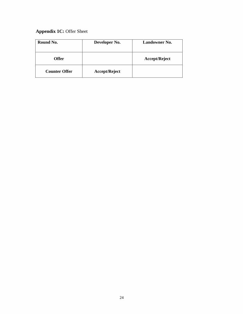
Appendix 1C: Offer Sheet Round No. Developer No. Landowner No.

Offer Accept/Reject

Counter Offer Accept/Reject

24

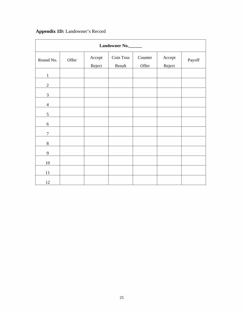
Appendix 1D: Landowner’s Record

Landowner No.______

Accept Coin Toss Counter Accept Round No. Offer Reject Result Offer Reject

Payoff

1

2

3

4

5

6

7

8

9

10

11

12

25

Appendix 1E: Developer’s Record

Developer No. _____

Round Landowner No. 1

Landowner No. 2

Landowner No. 3

No. Sequence Offer Accept Counter Accept Sequence Offer Accept Counter Accept Sequence Offer Accept Counter Accept Developer

Reject Offer Reject Reject Offer Reject Reject Offer Reject Gain

1

2

3

4

5

6

7

8

9

10

26

References

Binmore, Kenneth, Avnner Shaked, and John Sutton, “Testing noncooperative

bargaining theory: A preliminary study,” American Economic Review, 1985, 75,

1175–1180.

Cai, Hongbin, “Delay in multilateral bargaining under complete information,” Journal

of Economic Theory, 8 2000, 93 (2), 260–276.

Camerer, Colin, Behavioral Game Theory, Princeton University Press, 2003.

Coase, Ronald, “The problem of social cost,” Journal of Law and Economics, 1961, 3,

1–44.

Furusawa, Taiji and Quan Wen, “Unique inefficient perfect equilibrium in a stochas-

tic model of bargaining with complete information,” 1999. University of Windsor

working paper.

Grossman, Sanford and Motty Perry, “Sequential bargaining under asymmetric

information,” Journal of Economic Theory, 1986, 39, 120–154.

Horn, Henrik and Asher Wolinsky, “Worker substitutability and patterns of union-

isation,” Economic Journal, 1988, 98 (127), 484–97.

Huyck, John G. Van, Frederick Rankin, and Raymond C. Battalio, “Tacit

cooperation, strategic uncertainty, and coordination failure: Evidence from repeated

dominance solvable games,” Games and Economic Behavior, 2002, 38, 156–175.

Johnson, Eric, Colin Camerer, Sankar Sen, and Talia Rymon, “Detecting fail-

ures of backward induction: Monitoring information search in sequential bargaining

experiments,” Journal of Economic Theory, 2002, 104, 16–47.

Marx, Leslie and Greg Shaffer, “Bargaining power in sequential contracting,” 2004.

Duke University working paper.

McAfee, R. Preston and Marius Schwartz, “Opportunism in multilateral vertical

contracting: Nondiscrimination, exclusivity and uniformity,” American Economic

Review, 1994, 84, 210–230.

McKelvey, Richard and Thomas Palfrey, “A experimental study of the centipede

game,” Econometrica, 1992, 60, 803–836.

27

Noe, Thomas and Jun Wang, “Strategic Debt Restructuring,” Review of Financial

Studies, 2000, 13, 985–1015.

and , “Fooling all of the people some of the time: A theory of endogenous

sequencing in confidential negotiations,” Review of Economic Studies, 2004, 71, 855–

881.

Ochs, Jack and Alvin Roth, “A experimental study of sequential bargaining,” Amer-

ican Economic Review, 1989, 79, 355–384.

Osborne, Martin and Ariel Rubinstein, Bargaining and Markets, New York, NY:

Academic Press, 1990.

Pigou, Arthur, The Economics of Welfare, McMillan & Co., 1920.

Roth, Alvin and Michael Malouf, “Game-theoretic models and the role of informa-

tion in bargaining,” Psychological Review, 1979, 86, 574–594.

Rubinstein, Ariel, “The electronic mail game: strategic behavior under almost common

knowledge,” American Economic Review, 1989, 79, 385–391.

Salmon, Timothy C., “An evaluation of econometric models of adaptive learning,”

Econometrica, 2001, 69, 1597–1628.

Sefton, Martin and Abdullah Yavas, “Abreu-Matsushima mechanisms: Experimen-

tal evidence,” Games and Economic Behavior, 1996, 16, 280–302.

Shintani, Toramatsu and Katia Sycara, “Multiple negotiations among agents for

a distributed meeting scheduler,” Fourth International Conference on MultiAgent

Systems (ICMAS-2000), 2000, pp. 435–436.

28

Table 1: Summary of Negotiation SuccessThis table presents the number of bilateral negotiations (N), successful ones (N Success),failed ones (N Failure), and percent of failed negotiations (% Failure). N1, N2, and N3represent the first, second, and third negotiation, respectively.

N N Success N Failure % FailureN1 60 48 12 20%N2 48 36 12 25%N3 36 33 3 8%ALL 60 33 27 45%

29

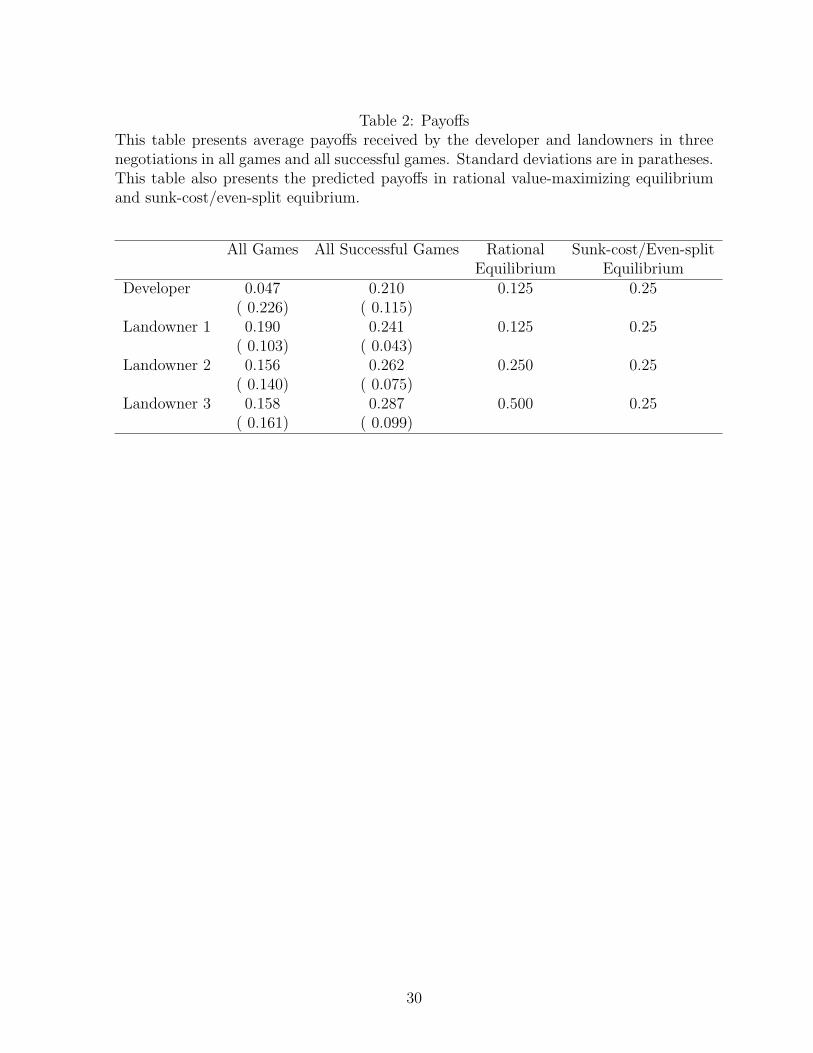
Table 2: PayoffsThis table presents average payoffs received by the developer and landowners in threenegotiations in all games and all successful games. Standard deviations are in paratheses.This table also presents the predicted payoffs in rational value-maximizing equilibriumand sunk-cost/even-split equibrium.

All Games All Successful Games Rational Sunk-cost/Even-splitEquilibrium Equilibrium

Developer 0.047 0.210 0.125 0.25( 0.226) ( 0.115)

Landowner 1 0.190 0.241 0.125 0.25( 0.103) ( 0.043)

Landowner 2 0.156 0.262 0.250 0.25( 0.140) ( 0.075)

Landowner 3 0.158 0.287 0.500 0.25( 0.161) ( 0.099)

30

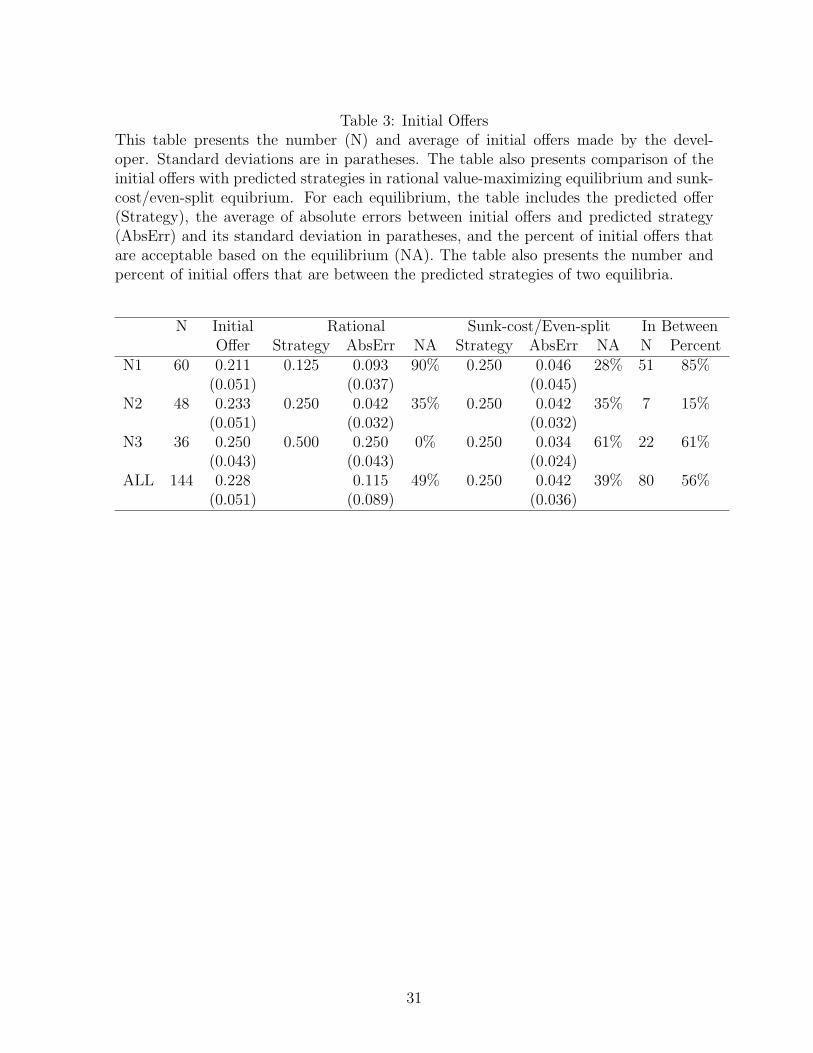
Table 3: Initial OffersThis table presents the number (N) and average of initial offers made by the devel-oper. Standard deviations are in paratheses. The table also presents comparison of theinitial offers with predicted strategies in rational value-maximizing equilibrium and sunk-cost/even-split equibrium. For each equilibrium, the table includes the predicted offer(Strategy), the average of absolute errors between initial offers and predicted strategy(AbsErr) and its standard deviation in paratheses, and the percent of initial offers thatare acceptable based on the equilibrium (NA). The table also presents the number andpercent of initial offers that are between the predicted strategies of two equilibria.

N Initial Rational Sunk-cost/Even-split In BetweenOffer Strategy AbsErr NA Strategy AbsErr NA N Percent

N1 60 0.211 0.125 0.093 90% 0.250 0.046 28% 51 85%(0.051) (0.037) (0.045)

N2 48 0.233 0.250 0.042 35% 0.250 0.042 35% 7 15%(0.051) (0.032) (0.032)

N3 36 0.250 0.500 0.250 0% 0.250 0.034 61% 22 61%(0.043) (0.043) (0.024)

ALL 144 0.228 0.115 49% 0.250 0.042 39% 80 56%(0.051) (0.089) (0.036)

31

Table 4: Acceptance Decision of Initial OffersThis table presents the number (N), average (Mean), and standard deviation (in parathe-ses) of initial offers that are accepted and rejected. The table also presents the percentof acceptable offers (NA) based on two equilibria, rational value-maximizing equilibriumand sunk-cost equilibrium. In addition, it provides the percent of acceptable offers basedon the equilibrium that are accepted (PA), and percent of rejectable offers based on theequilibrium that are rejected (PR).

Accepted Rejected Rational Sunk-cost/Even-splitN Mean N Mean NA PA PR NA PA PR

N1 42 0.227 18 0.174 90% 78% 100% 28% 82% 35%(0.034) (0.064)

N2 32 0.243 16 0.212 35% 76% 39% 35% 76% 39%(0.051) (0.045)

N3 28 0.255 8 0.231 0% 22% 61% 86% 36%(0.039) (0.051)

ALL 102 0.240 42 0.199 49% 77% 36% 39% 82% 36%(0.042) (0.058)

32

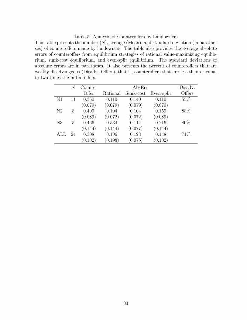
Table 5: Analysis of Counteroffers by LandownersThis table presents the number (N), average (Mean), and standard deviation (in parathe-ses) of counteroffers made by landowners. The table also provides the average absoluteerrors of counteroffers from equilibrium strategies of rational value-maximizing equilib-rium, sunk-cost equilibrium, and even-split equilibrium. The standard deviations ofabsolute errors are in paratheses. It also presents the percent of counteroffers that areweakly disadvangeous (Disadv. Offers), that is, counteroffers that are less than or equalto two times the initial offers.

N Counter AbsErr Disadv.Offer Rational Sunk-cost Even-split Offers

N1 11 0.360 0.110 0.140 0.110 55%(0.079) (0.079) (0.079) (0.079)

N2 8 0.409 0.104 0.104 0.159 88%(0.089) (0.072) (0.072) (0.089)

N3 5 0.466 0.534 0.114 0.216 80%(0.144) (0.144) (0.077) (0.144)

ALL 24 0.398 0.196 0.123 0.148 71%(0.102) (0.198) (0.075) (0.102)

33

Table 6: Acceptance Decision of the DeveloperThis table presents the number (N), average (Mean), and standard deviation (in parathe-ses) of counteroffers that are accepted and rejected. The table also presents the percent ofacceptable counteroffers (NA) based on two equilibria, rational equilibrium and sunk-costequilibrium. In addition, it provides the percent of acceptable offers based on the equi-librium that are accepted (PA), and percent of rejectable offers based on the equilibriumthat are rejected (PR).

Accepted Rejected Rational Sunk-cost/Even-splitN Mean N Mean NA PA PR NA PA PR

N1 6 0.310 5 0.420 0% - 45% 100% 55% -(0.015) (0.084)

N2 4 0.390 4 0.428 88% 57% 100% 88% 57% 100%(0.099) (0.088)

N3 5 0.466 100% 100% - 60% 100% 0%(0.144)

ALL 15 0.383 9 0.423 50% 75% 50% 88% 62% 33%(0.113) (0.080)

34

Table 7: Ananlysis of Learning by Developers in Making Initial OffersThis table presents the number (N), average (Mean), and standard deviation (Std) ofthe difference between two initial offers of the same negotiaion of two consequtive gamesconditional on whether the offer in the last game is accepted. The table also presents tstatistics (t-stat) on tests of whether the means of the two subsamples are equal.

Offer Difference between Two Consequetive GamesLast offer accepted Last offer rejected

N Mean Std N Mean Std t-statPanel A. All

N1 39 -0.016 0.059 18 0.036 0.059 -3.06N2 30 -0.014 0.041 15 0.032 0.070 -2.77N3 26 -0.000 0.046 7 0.029 0.071 -1.30

Panel B. Excluding consequetive games that aremore than two games apart

N2 28 -0.013 0.042 14 0.031 0.072 -2.48N3 21 -0.004 0.045 6 0.050 0.047 -2.56

35

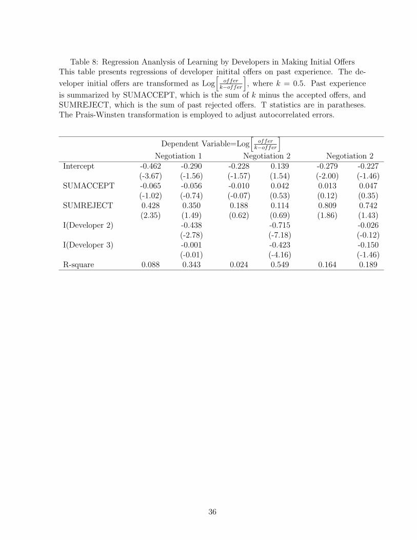
Table 8: Regression Ananlysis of Learning by Developers in Making Initial OffersThis table presents regressions of developer initital offers on past experience. The de-

veloper initial offers are transformed as Log[

offerk−offer

], where k = 0.5. Past experience

is summarized by SUMACCEPT, which is the sum of k minus the accepted offers, andSUMREJECT, which is the sum of past rejected offers. T statistics are in paratheses.The Prais-Winsten transformation is employed to adjust autocorrelated errors.

Dependent Variable=Log[

offerk−offer

]Negotiation 1 Negotiation 2 Negotiation 2

Intercept -0.462 -0.290 -0.228 0.139 -0.279 -0.227(-3.67) (-1.56) (-1.57) (1.54) (-2.00) (-1.46)

SUMACCEPT -0.065 -0.056 -0.010 0.042 0.013 0.047(-1.02) (-0.74) (-0.07) (0.53) (0.12) (0.35)

SUMREJECT 0.428 0.350 0.188 0.114 0.809 0.742(2.35) (1.49) (0.62) (0.69) (1.86) (1.43)

I(Developer 2) -0.438 -0.715 -0.026(-2.78) (-7.18) (-0.12)

I(Developer 3) -0.001 -0.423 -0.150(-0.01) (-4.16) (-1.46)

R-square 0.088 0.343 0.024 0.549 0.164 0.189

36

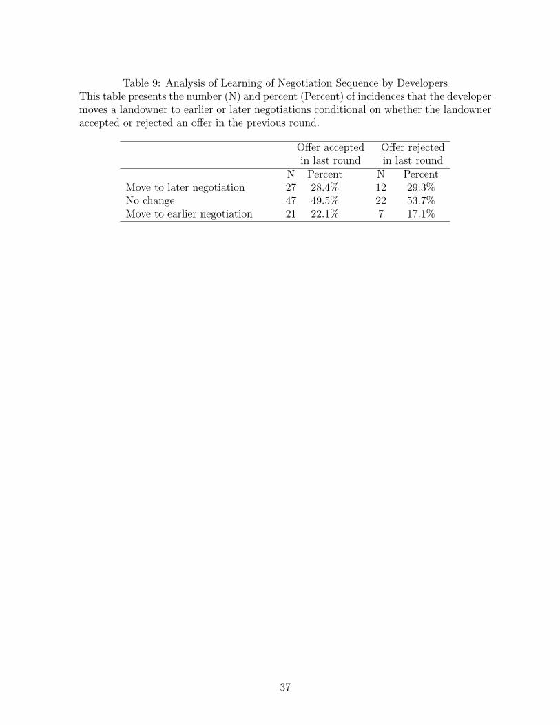
Table 9: Analysis of Learning of Negotiation Sequence by DevelopersThis table presents the number (N) and percent (Percent) of incidences that the developermoves a landowner to earlier or later negotiations conditional on whether the landowneraccepted or rejected an offer in the previous round.

Offer accepted Offer rejectedin last round in last round

N Percent N PercentMove to later negotiation 27 28.4% 12 29.3%No change 47 49.5% 22 53.7%Move to earlier negotiation 21 22.1% 7 17.1%

37