Business Statistics - Unit 2 - Probability
132
Business Statistics - Unit 2 - Probability Collection Editor: Collette Lemieux
Transcript of Business Statistics - Unit 2 - Probability
Business Statistics - Unit 2 - Probability
Collection Editor:Collette Lemieux

Business Statistics - Unit 2 - Probability
Collection Editor:Collette Lemieux
Authors:OpenStax
Lyryx LearningCollette Lemieux
Online:< http://cnx.org/content/col12245/1.3/ >

This selection and arrangement of content as a collection is copyrighted by Collette Lemieux. It is licensed under theCreative Commons Attribution License 4.0 (http://creativecommons.org/licenses/by/4.0/).Collection structure revised: September 20, 2017PDF generated: October 6, 2020For copyright and attribution information for the modules contained in this collection, see p. 123.
Table of Contents
1 Chapter 3 - Probability Topics
1.1 Introduction � Probability Topics � MtRoyal - Version2016RevA . . . . . . . . . . . . . . . . . . . . . . . . . . . . . 11.2 Terminology � Probability Topics � MtRoyal - Version2016RevA . . . . . . . . . . . . . . . . . . . . . . . . . . . . . 21.3 Independent and Mutually Exclusive Events � Probaility Topics � MtRoyal -
Version2016RevA . . . . . . . . . . . . . . . . . . . . . . . . . . . . . . . . . . . . . . . . . . . . . . . . . . . . . . . . . . . . . . . . . . . . . . . . . . . 131.4 Two Basic Rules of Probability . . . . . . . . . . . . . . . . . . . . . . . . . . . . . . . . . . . . . . . . . . . . . . . . . . . . . . . . . . . . . 251.5 Contingency Tables and Tree Diagrams � Probability Topics � MtRoyal - Ver-
sion2016RevA . . . . . . . . . . . . . . . . . . . . . . . . . . . . . . . . . . . . . . . . . . . . . . . . . . . . . . . . . . . . . . . . . . . . . . . . . . . . . . 39Solutions . . . . . . . . . . . . . . . . . . . . . . . . . . . . . . . . . . . . . . . . . . . . . . . . . . . . . . . . . . . . . . . . . . . . . . . . . . . . . . . . . . . . . . . . 53
2 Chapter 4 - Binomial Distribution
2.1 Introduction to Discrete Probability Distributions - MRU - C Lemieux (2017) . . . . . . . . . . . . . . 612.2 Binomial distribution - MRU - C Lemieux . . . . . . . . . . . . . . . . . . . . . . . . . . . . . . . . . . . . . . . . . . . . . . . . . . 62Solutions . . . . . . . . . . . . . . . . . . . . . . . . . . . . . . . . . . . . . . . . . . . . . . . . . . . . . . . . . . . . . . . . . . . . . . . . . . . . . . . . . . . . . . . . 74
3 Chapter 5 - Normal Distribution
3.1 Introduction � The Normal Distribution � Mt Royal University � Version2016RevA . . . . . . . . . . . . . . . . . . . . . . . . . . . . . . . . . . . . . . . . . . . . . . . . . . . . . . . . . . . . . . . . . . . . . . . . . . . . . . . . . . 83
3.2 The Standard Normal Distribution� The Normal Distribution �MRU - C Lemieux . . . . . . . . . . . . . 853.3 Using the Normal Distribution� The Normal Distribution � MRU - C Lemieux .. . . . . . . . . . . . . 90Solutions . . . . . . . . . . . . . . . . . . . . . . . . . . . . . . . . . . . . . . . . . . . . . . . . . . . . . . . . . . . . . . . . . . . . . . . . . . . . . . . . . . . . . . . 102
4 Chapter 6 - Sampling Distribution
4.1 Introduction - Sampling distributions - MRU - C Lemieux . . . . . . . . . . . . . . . . . . . . . . . . . . . . . . . . . 1034.2 Introduction to Sampling Distributions . . . . . . . . . . . . . . . . . . . . . . . . . . . . . . . . . . . . . . . . . . . . . . . . . . . . 1034.3 Constructing empirical sampling distributions - MRU - C Lemieux . . . . . . . . . . . . .. . . . . . . . . . . . 1054.4 Central Limit Theorem - MRU - C Lemieux . . . . . . . . . . . . . . . . . . . . . . . . . . . . . . . . . . . . . . . . . . . . . . . 1084.5 A series of examples - Calculating probabilities for sampling distributions - MRU
- C Lemieux . . . . . . . . . . . . . . . . . . . . . . . . . . . . . . . . . . . . . . . . . . . . . . . . . . . . . . . . . . . . . . . . . . . . . . . . . . . . . . . 114Solutions . . . . . . . . . . . . . . . . . . . . . . . . . . . . . . . . . . . . . . . . . . . . . . . . . . . . . . . . . . . . . . . . . . . . . . . . . . . . . . . . . . . . . . . 118
Glossary . . . . . . . . . . . . . . . . . . . . . . . . . . . . . . . . . . . . . . . . . . . . . . . . . . . . . . . . . . . . . . . . . . . . . . . . . . . . . . . . . . . . . . . . . . . . 120Index . . . . . . . . . . . . . . . . . . . . . . . . . . . . . . . . . . . . . . . . . . . . . . . . . . . . . . . . . . . . . . . . . . . . . . . . . . . . . . . . . . . . . . . . . . . . . . . 122Attributions . . . . . . . . . . . . . . . . . . . . . . . . . . . . . . . . . . . . . . . . . . . . . . . . . . . . . . . . . . . . . . . . . . . . . . . . . . . . . . . . . . . . . . . .123

iv
Available for free at Connexions <http://cnx.org/content/col12245/1.3>
Chapter 1
Chapter 3 - Probability Topics
1.1 Introduction � Probability Topics � MtRoyal - Version2016RevA1
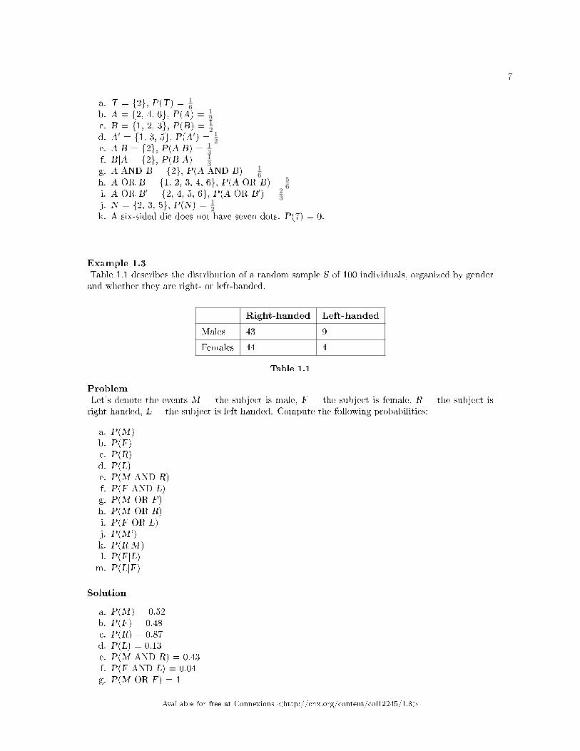
Figure 1.1: Meteor showers are rare, but the probability of them occurring can be calculated. (credit:Navicore/�ickr)
: By the end of this chapter, the student should be able to:
• Understand and use the terminology of probability.• Determine whether two events are mutually exclusive and whether two events are independent.• Calculate probabilities using the addition and multiplication rules.• Construct and interpret contingency tables and tree diagrams.• Understand the di�erence between likely and unlikely events.
1This content is available online at <http://cnx.org/content/m62328/1.1/>.
Available for free at Connexions <http://cnx.org/content/col12245/1.3>
1
2 CHAPTER 1. CHAPTER 3 - PROBABILITY TOPICS
It is often necessary to "guess" about the outcome of an event in order to make a decision. Politicians studypolls to guess their likelihood of winning an election. Teachers choose a particular course of study based onwhat they think students can comprehend. Doctors choose the treatments needed for various diseases basedon their assessment of likely results. You may have visited a casino where people play games chosen becauseof the belief that the likelihood of winning is good. You may have chosen your course of study based on theprobable availability of jobs.
You have, more than likely, used probability. In fact, you probably have an intuitive sense of probability.Probability deals with the chance of an event occurring. Whenever you weigh the odds of whether or not todo your homework or to study for an exam, you are using probability. In this chapter, you will learn how tosolve probability problems using a systematic approach.
1.2 Terminology � Probability Topics � MtRoyal - Version2016RevA2
Probability is a measure that is associated with how certain we are of outcomes of a particular experimentor activity. An experiment is a planned operation carried out under controlled conditions. If the result isnot predetermined, then the experiment is said to be a chance experiment. Flipping one fair coin twice isan example of an experiment.
A result of an experiment is called an outcome. The sample space of an experiment is the set of allpossible outcomes. Three ways to represent a sample space are: to list the possible outcomes, to create atree diagram, or to create a Venn diagram. The uppercase letter S is used to denote the sample space. Forexample, if you �ip one fair coin, S = {H, T} where H = heads and T = tails are the outcomes.
An event is any combination of outcomes. Upper case letters like A and B represent events. For example,if the experiment is to �ip one fair coin, event A might be getting at most one head. The probability of anevent A is written P(A).
The probability of any outcome is the long-term relative frequency of that outcome. Probabilitiesare between zero and one, inclusive (that is, zero and one and all numbers between these values). P(A)= 0 means the event A can never happen. P(A) = 1 means the event A always happens. P(A) = 0.5 meansthat event A has a 50% chance of happening. For example, if you �ip one fair coin repeatedly (from 20 to2,000 to 20,000 times) the relative frequency of heads approaches 0.5 (the probability of heads).
Equally likely means that each outcome of an experiment occurs with equal probability. For example,if you toss a fair, six-sided die, each face (1, 2, 3, 4, 5, or 6) is as likely to occur as any other face. If youtoss a fair coin, a Head (H) and a Tail (T) are equally likely to occur. If you randomly guess the answer toa true/false question on an exam, you are equally likely to select a correct answer or an incorrect answer.
To calculate the probability of an event A when all outcomes in the sample space are equallylikely, count the number of outcomes for event A and divide by the total number of outcomes in the samplespace. For example, if you toss a fair dime and a fair nickel, the sample space is {HH, TH, HT, TT} whereT = tails and H = heads. The sample space has four outcomes. A = getting one head. There are twooutcomes that meet this condition {HT, TH}, so P(A) = 2
4 = 0.5.Suppose you roll one fair six-sided die, with the numbers {1, 2, 3, 4, 5, 6} on its faces. Let event E =
rolling a number that is at least �ve. There are two outcomes {5, 6}. P(E) = 26 . If you were to roll the
die only a few times, you would not be surprised if your observed results did not match the probability. Ifyou were to roll the die a very large number of times, you would expect that, overall, 2
6 of the rolls wouldresult in an outcome of "at least �ve". You would not expect exactly 2
6 . The long-term relative frequencyof obtaining this result would approach the theoretical probability of 2
6 as the number of repetitions growslarger and larger.
This important characteristic of probability experiments is known as the law of large numbers whichstates that as the number of repetitions of an experiment is increased, the relative frequency obtained inthe experiment tends to become closer and closer to the theoretical probability. Even though the outcomes
2This content is available online at <http://cnx.org/content/m62337/1.3/>.
Available for free at Connexions <http://cnx.org/content/col12245/1.3>
3
do not happen according to any set pattern or order, overall, the long-term observed relative frequency willapproach the theoretical probability. (The word empirical is often used instead of the word observed.)
It is important to realize that in many situations, the outcomes are not equally likely. A coin or die maybe unfair, or biased. Two math professors in Europe had their statistics students test the Belgian oneEuro coin and discovered that in 250 trials, a head was obtained 56% of the time and a tail was obtained44% of the time. The data seem to show that the coin is not a fair coin; more repetitions would be helpfulto draw a more accurate conclusion about such bias. Some dice may be biased. Look at the dice in a gameyou have at home; the spots on each face are usually small holes carved out and then painted to make thespots visible. Your dice may or may not be biased; it is possible that the outcomes may be a�ected by theslight weight di�erences due to the di�erent numbers of holes in the faces. Gambling casinos make a lotof money depending on outcomes from rolling dice, so casino dice are made di�erently to eliminate bias.Casino dice have �at faces; the holes are completely �lled with paint having the same density as the materialthat the dice are made out of so that each face is equally likely to occur. Later we will learn techniques touse to work with probabilities for events that are not equally likely.
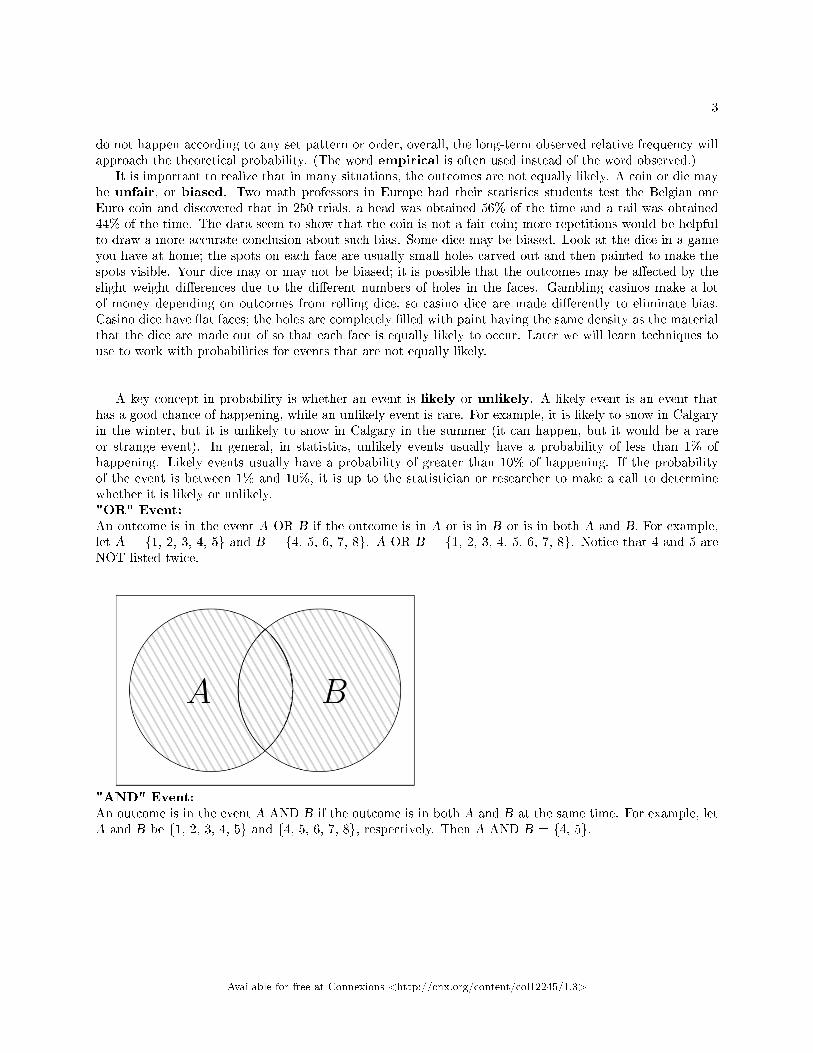
A key concept in probability is whether an event is likely or unlikely. A likely event is an event thathas a good chance of happening, while an unlikely event is rare. For example, it is likely to snow in Calgaryin the winter, but it is unlikely to snow in Calgary in the summer (it can happen, but it would be a rareor strange event). In general, in statistics, unlikely events usually have a probability of less than 1% ofhappening. Likely events usually have a probability of greater than 10% of happening. If the probabilityof the event is between 1% and 10%, it is up to the statistician or researcher to make a call to determinewhether it is likely or unlikely."OR" Event:An outcome is in the event A OR B if the outcome is in A or is in B or is in both A and B. For example,let A = {1, 2, 3, 4, 5} and B = {4, 5, 6, 7, 8}. A OR B = {1, 2, 3, 4, 5, 6, 7, 8}. Notice that 4 and 5 areNOT listed twice.
"AND" Event:An outcome is in the event A AND B if the outcome is in both A and B at the same time. For example, letA and B be {1, 2, 3, 4, 5} and {4, 5, 6, 7, 8}, respectively. Then A AND B = {4, 5}.
Available for free at Connexions <http://cnx.org/content/col12245/1.3>
4 CHAPTER 1. CHAPTER 3 - PROBABILITY TOPICS
The complement of event A is denoted A′ (read "A prime"). A′ consists of all outcomes that are NOTin A. Notice that P(A) + P(A′) = 1. For example, let S = {1, 2, 3, 4, 5, 6} and let A = {1, 2, 3, 4}. Then,A′ = {5, 6}. P(A) = 4
6 , P(A′) = 2
6 , and P(A) + P(A′) = 46 + 2
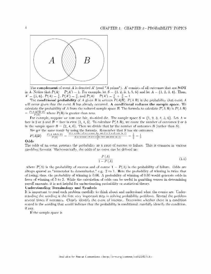
6 = 1The conditional probability of A given B is written P(A|B). P(A|B) is the probability that event A
will occur given that the event B has already occurred. A conditional reduces the sample space. Wecalculate the probability of A from the reduced sample space B. The formula to calculate P(A|B) is P(A|B)
= P (A AND B)P (B) where P(B) is greater than zero.
For example, suppose we toss one fair, six-sided die. The sample space S = {1, 2, 3, 4, 5, 6}. Let A =face is 2 or 3 and B = face is even (2, 4, 6). To calculate P(A|B), we count the number of outcomes 2 or 3in the sample space B = {2, 4, 6}. Then we divide that by the number of outcomes B (rather than S).
We get the same result by using the formula. Remember that S has six outcomes.
P(A|B) = P (A AND B)P (B) =
(the number of outcomes that are 2 or 3 and even in S)6
(the number of outcomes that are even in S)6
=1636
= 13
OddsThe odds of an event presents the probability as a ratio of success to failure. This is common in variousgambling formats. Mathematically, the odds of an event can be de�ned as:
P (A)
1− P (A)(1.1)
where P(A) is the probability of success and of course 1 − P(A) is the probability of failure. Odds arealways quoted as "numerator to denominator," e.g. 2 to 1. Here the probability of winning is twice thatof losing; thus, the probability of winning is 0.66. A probability of winning of 0.60 would generate odds infavor of winning of 3 to 2. While the calculation of odds can be useful in gambling venues in determiningpayo� amounts, it is not helpful for understanding probability or statistical theory.Understanding Terminology and SymbolsIt is important to read each problem carefully to think about and understand what the events are. Under-standing the wording is the �rst very important step in solving probability problems. Reread the problemseveral times if necessary. Clearly identify the event of interest. Determine whether there is a conditionstated in the wording that would indicate that the probability is conditional; carefully identify the condition,if any.
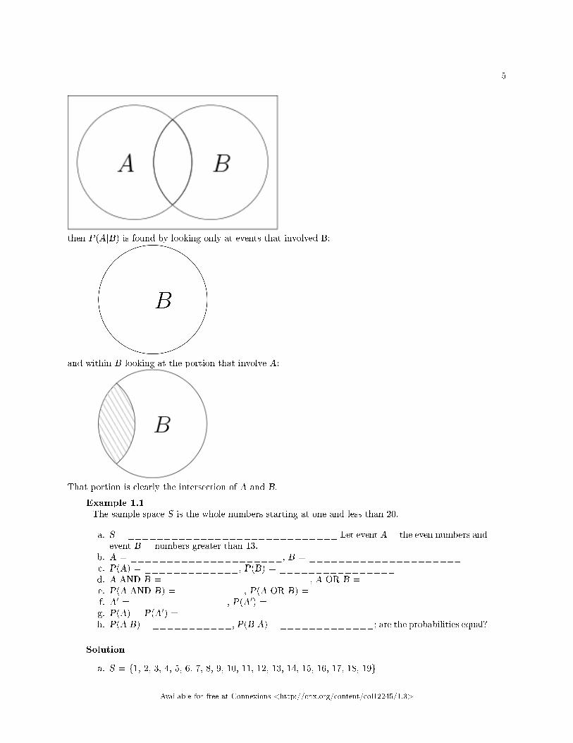
If the sample space is
Available for free at Connexions <http://cnx.org/content/col12245/1.3>
5
then P(A|B) is found by looking only at events that involved B:
and within B looking at the portion that involve A:
That portion is clearly the intersection of A and B.
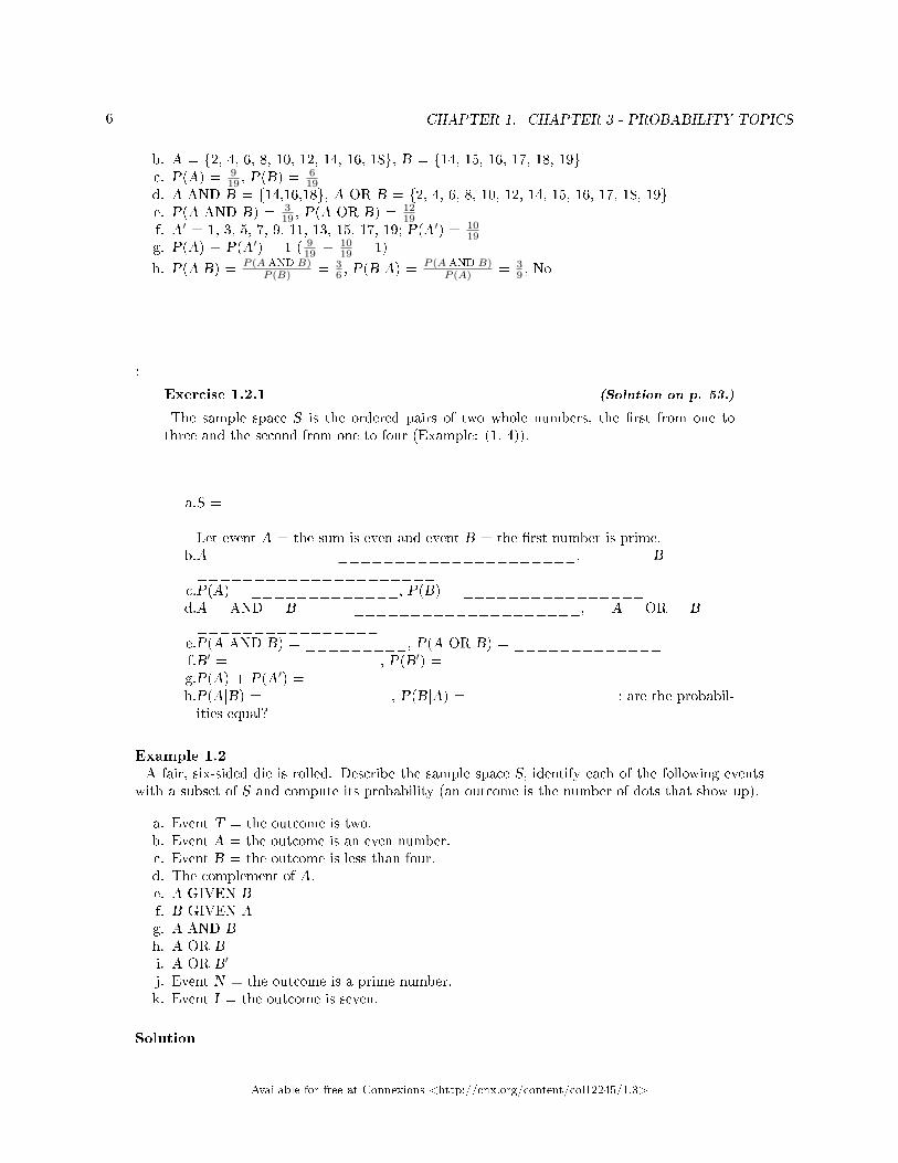
Example 1.1The sample space S is the whole numbers starting at one and less than 20.
a. S = _____________________________ Let event A = the even numbers andevent B = numbers greater than 13.
b. A = _____________________, B = _____________________c. P(A) = _____________, P(B) = ________________d. A AND B = ____________________, A OR B = ________________e. P(A AND B) = _________, P(A OR B) = _____________f. A′ = _____________, P(A′) = _____________g. P(A) + P(A′) = ____________h. P(A|B) = ___________, P(B|A) = _____________; are the probabilities equal?
Solution
a. S = {1, 2, 3, 4, 5, 6, 7, 8, 9, 10, 11, 12, 13, 14, 15, 16, 17, 18, 19}
Available for free at Connexions <http://cnx.org/content/col12245/1.3>
6 CHAPTER 1. CHAPTER 3 - PROBABILITY TOPICS
b. A = {2, 4, 6, 8, 10, 12, 14, 16, 18}, B = {14, 15, 16, 17, 18, 19}c. P(A) = 9
19 , P(B) =619
d. A AND B = {14,16,18}, A OR B = {2, 4, 6, 8, 10, 12, 14, 15, 16, 17, 18, 19}e. P(A AND B) = 3
19 , P(A OR B) = 1219
f. A′ = 1, 3, 5, 7, 9, 11, 13, 15, 17, 19; P(A′) = 1019
g. P(A) + P(A′) = 1 ( 919 + 10
19 = 1)
h. P(A|B) = P (A AND B)P (B) = 3
6 , P(B|A) =P (A AND B)
P (A) = 39 , No
:
Exercise 1.2.1 (Solution on p. 53.)
The sample space S is the ordered pairs of two whole numbers, the �rst from one tothree and the second from one to four (Example: (1, 4)).
a.S = _____________________________
Let event A = the sum is even and event B = the �rst number is prime.b.A = _____________________, B =_____________________
c.P(A) = _____________, P(B) = ________________d.A AND B = ____________________, A OR B =________________
e.P(A AND B) = _________, P(A OR B) = _____________f.B′ = _____________, P(B′) = _____________g.P(A) + P(A′) = ____________h.P(A|B) = ___________, P(B|A) = _____________; are the probabil-ities equal?
Example 1.2A fair, six-sided die is rolled. Describe the sample space S, identify each of the following events
with a subset of S and compute its probability (an outcome is the number of dots that show up).
a. Event T = the outcome is two.b. Event A = the outcome is an even number.c. Event B = the outcome is less than four.d. The complement of A.e. A GIVEN Bf. B GIVEN Ag. A AND Bh. A OR Bi. A OR B′
j. Event N = the outcome is a prime number.k. Event I = the outcome is seven.
Solution
Available for free at Connexions <http://cnx.org/content/col12245/1.3>
7
a. T = {2}, P(T) = 16
b. A = {2, 4, 6}, P(A) = 12
c. B = {1, 2, 3}, P(B) = 12
d. A′ = {1, 3, 5}, P(A′) = 12
e. A|B = {2}, P(A|B) = 13
f. B|A = {2}, P(B|A) = 13
g. A AND B = {2}, P(A AND B) = 16
h. A OR B = {1, 2, 3, 4, 6}, P(A OR B) = 56
i. A OR B′ = {2, 4, 5, 6}, P(A OR B′) = 23
j. N = {2, 3, 5}, P(N) = 12
k. A six-sided die does not have seven dots. P(7) = 0.
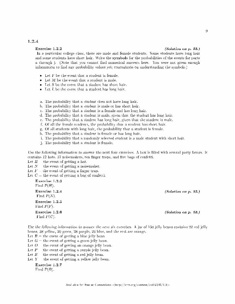
Example 1.3Table 1.1 describes the distribution of a random sample S of 100 individuals, organized by genderand whether they are right- or left-handed.
Right-handed Left-handed
Males 43 9
Females 44 4
Table 1.1
ProblemLet's denote the events M = the subject is male, F = the subject is female, R = the subject isright-handed, L = the subject is left-handed. Compute the following probabilities:
a. P(M)b. P(F)c. P(R)d. P(L)e. P(M AND R)f. P(F AND L)g. P(M OR F)h. P(M OR R)i. P(F OR L)j. P(M')k. P(R|M)l. P(F|L)m. P(L|F)
Solution
a. P(M) = 0.52b. P(F) = 0.48c. P(R) = 0.87d. P(L) = 0.13e. P(M AND R) = 0.43f. P(F AND L) = 0.04g. P(M OR F) = 1
Available for free at Connexions <http://cnx.org/content/col12245/1.3>
8 CHAPTER 1. CHAPTER 3 - PROBABILITY TOPICS
h. P(M OR R) = 0.96i. P(F OR L) = 0.57j. P(M') = 0.48k. P(R|M) = 0.8269 (rounded to four decimal places)l. P(F|L) = 0.3077 (rounded to four decimal places)m. P(L|F) = 0.0833
1.2.1 References
�Countries List by Continent.� Worldatlas, 2013. Available online athttp://www.worldatlas.com/cntycont.htm (accessed May 2, 2013).
1.2.2 Chapter Review
In this module we learned the basic terminology of probability. The set of all possible outcomes of anexperiment is called the sample space. Events are subsets of the sample space, and they are assigned aprobability that is a number between zero and one, inclusive.
1.2.3 Formula Review
A and B are eventsP(S) = 1 where S is the sample space0 ≤ P(A) ≤ 1
P(A|B) = P (A∩B)P (B)
Available for free at Connexions <http://cnx.org/content/col12245/1.3>
9
1.2.4
Exercise 1.2.2 (Solution on p. 53.)
In a particular college class, there are male and female students. Some students have long hairand some students have short hair. Write the symbols for the probabilities of the events for partsa through j. (Note that you cannot �nd numerical answers here. You were not given enoughinformation to �nd any probability values yet; concentrate on understanding the symbols.)
• Let F be the event that a student is female.• Let M be the event that a student is male.• Let S be the event that a student has short hair.• Let L be the event that a student has long hair.
a. The probability that a student does not have long hair.b. The probability that a student is male or has short hair.c. The probability that a student is a female and has long hair.d. The probability that a student is male, given that the student has long hair.e. The probability that a student has long hair, given that the student is male.f. Of all the female students, the probability that a student has short hair.g. Of all students with long hair, the probability that a student is female.h. The probability that a student is female or has long hair.i. The probability that a randomly selected student is a male student with short hair.j. The probability that a student is female.
Use the following information to answer the next four exercises. A box is �lled with several party favors. Itcontains 12 hats, 15 noisemakers, ten �nger traps, and �ve bags of confetti.Let H = the event of getting a hat.Let N = the event of getting a noisemaker.Let F = the event of getting a �nger trap.Let C = the event of getting a bag of confetti.
Exercise 1.2.3Find P(H).
Exercise 1.2.4 (Solution on p. 53.)
Find P(N).
Exercise 1.2.5Find P(F).
Exercise 1.2.6 (Solution on p. 53.)
Find P(C).
Use the following information to answer the next six exercises. A jar of 150 jelly beans contains 22 red jellybeans, 38 yellow, 20 green, 28 purple, 26 blue, and the rest are orange.Let B = the event of getting a blue jelly beanLet G = the event of getting a green jelly bean.Let O = the event of getting an orange jelly bean.Let P = the event of getting a purple jelly bean.Let R = the event of getting a red jelly bean.Let Y = the event of getting a yellow jelly bean.
Exercise 1.2.7Find P(B).
Available for free at Connexions <http://cnx.org/content/col12245/1.3>
10 CHAPTER 1. CHAPTER 3 - PROBABILITY TOPICS
Exercise 1.2.8 (Solution on p. 53.)
Find P(G).
Exercise 1.2.9Find P(P).
Exercise 1.2.10 (Solution on p. 53.)
Find P(R).
Exercise 1.2.11Find P(Y ).
Exercise 1.2.12 (Solution on p. 53.)
Find P(O).
Use the following information to answer the next six exercises. There are 23 countries in North America, 12countries in South America, 47 countries in Europe, 44 countries in Asia, 54 countries in Africa, and 14 inOceania (Paci�c Ocean region).Let A = the event that a country is in Asia.Let E = the event that a country is in Europe.Let F = the event that a country is in Africa.Let N = the event that a country is in North America.Let O = the event that a country is in Oceania.Let S = the event that a country is in South America.
Exercise 1.2.13Find P(A).
Exercise 1.2.14 (Solution on p. 53.)
Find P(E).
Exercise 1.2.15Find P(F).
Exercise 1.2.16 (Solution on p. 53.)
Find P(N).
Exercise 1.2.17Find P(O).
Exercise 1.2.18 (Solution on p. 53.)
Find P(S).
Exercise 1.2.19What is the probability of drawing a red card in a standard deck of 52 cards?
Exercise 1.2.20 (Solution on p. 53.)
What is the probability of drawing a club in a standard deck of 52 cards?
Exercise 1.2.21What is the probability of rolling an even number of dots with a fair, six-sided die numbered onethrough six?
Exercise 1.2.22 (Solution on p. 53.)
What is the probability of rolling a prime number of dots with a fair, six-sided die numbered onethrough six?
Use the following information to answer the next two exercises. You see a game at a local fair. You have tothrow a dart at a color wheel. Each section on the color wheel is equal in area.
Available for free at Connexions <http://cnx.org/content/col12245/1.3>

11
Figure 1.2
Let B = the event of landing on blue.Let R = the event of landing on red.Let G = the event of landing on green.Let Y = the event of landing on yellow.
Exercise 1.2.23If you land on Y, you get the biggest prize. Find P(Y ).
Exercise 1.2.24 (Solution on p. 53.)
If you land on red, you don't get a prize. What is P(R)?
Use the following information to answer the next ten exercises. On a baseball team, there are in�elders andout�elders. Some players are great hitters, and some players are not great hitters.Let I = the event that a player in an in�elder.Let O = the event that a player is an out�elder.Let H = the event that a player is a great hitter.Let N = the event that a player is not a great hitter.
Exercise 1.2.25Write the symbols for the probability that a player is not an out�elder.
Exercise 1.2.26 (Solution on p. 53.)
Write the symbols for the probability that a player is an out�elder or is a great hitter.
Exercise 1.2.27Write the symbols for the probability that a player is an in�elder and is not a great hitter.
Available for free at Connexions <http://cnx.org/content/col12245/1.3>
12 CHAPTER 1. CHAPTER 3 - PROBABILITY TOPICS
Exercise 1.2.28 (Solution on p. 54.)
Write the symbols for the probability that a player is a great hitter, given that the player is anin�elder.
Exercise 1.2.29Write the symbols for the probability that a player is an in�elder, given that the player is a greathitter.
Exercise 1.2.30 (Solution on p. 54.)
Write the symbols for the probability that of all the out�elders, a player is not a great hitter.
Exercise 1.2.31Write the symbols for the probability that of all the great hitters, a player is an out�elder.
Exercise 1.2.32 (Solution on p. 54.)
Write the symbols for the probability that a player is an in�elder or is not a great hitter.
Exercise 1.2.33Write the symbols for the probability that a player is an out�elder and is a great hitter.
Exercise 1.2.34 (Solution on p. 54.)
Write the symbols for the probability that a player is an in�elder.
Exercise 1.2.35What is the word for the set of all possible outcomes?
Exercise 1.2.36 (Solution on p. 54.)
What is conditional probability?
Exercise 1.2.37A shelf holds 12 books. Eight are �ction and the rest are non�ction. Each is a di�erent book witha unique title. The �ction books are numbered one to eight. The non�ction books are numberedone to four. Randomly select one bookLet F = event that book is �ctionLet N = event that book is non�ctionWhat is the sample space?
Exercise 1.2.38 (Solution on p. 54.)
What is the sum of the probabilities of an event and its complement?
Use the following information to answer the next two exercises. You are rolling a fair, six-sided number cube.Let E = the event that it lands on an even number. Let M = the event that it lands on a multiple of three.
Exercise 1.2.39What does P(E|M) mean in words?
Exercise 1.2.40 (Solution on p. 54.)
What does P(E OR M) mean in words?
1.2.5 Homework
Exercise 1.2.41
Available for free at Connexions <http://cnx.org/content/col12245/1.3>
13
Figure 1.3
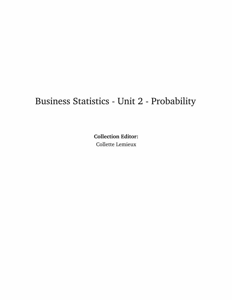
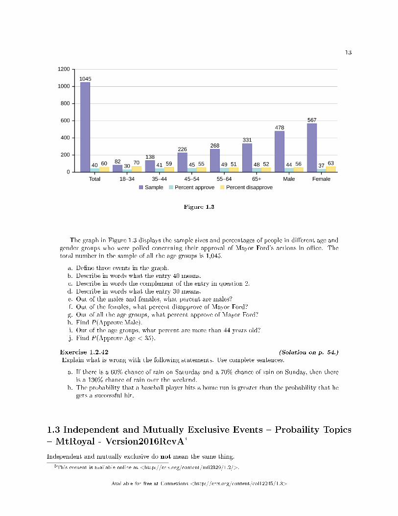
The graph in Figure 1.3 displays the sample sizes and percentages of people in di�erent age andgender groups who were polled concerning their approval of Mayor Ford's actions in o�ce. Thetotal number in the sample of all the age groups is 1,045.
a. De�ne three events in the graph.b. Describe in words what the entry 40 means.c. Describe in words the complement of the entry in question 2.d. Describe in words what the entry 30 means.e. Out of the males and females, what percent are males?f. Out of the females, what percent disapprove of Mayor Ford?g. Out of all the age groups, what percent approve of Mayor Ford?h. Find P(Approve|Male).i. Out of the age groups, what percent are more than 44 years old?j. Find P(Approve|Age < 35).
Exercise 1.2.42 (Solution on p. 54.)
Explain what is wrong with the following statements. Use complete sentences.
a. If there is a 60% chance of rain on Saturday and a 70% chance of rain on Sunday, then thereis a 130% chance of rain over the weekend.
b. The probability that a baseball player hits a home run is greater than the probability that hegets a successful hit.
1.3 Independent and Mutually Exclusive Events � Probaility Topics� MtRoyal - Version2016RevA3
Independent and mutually exclusive do not mean the same thing.
3This content is available online at <http://cnx.org/content/m62329/1.2/>.
Available for free at Connexions <http://cnx.org/content/col12245/1.3>
14 CHAPTER 1. CHAPTER 3 - PROBABILITY TOPICS
1.3.1 Independent Events
Two events are independent if the following are true:
• P(A|B) = P(A)• P(B|A) = P(B)• P(A AND B) = P(A)P(B)
Two events A and B are independent if the knowledge that one occurred does not a�ect the chance theother occurs. For example, the outcomes of two roles of a fair die are independent events. The outcome ofthe �rst roll does not change the probability for the outcome of the second roll. To show two events areindependent, you must show only one of the above conditions. If two events are NOT independent, thenwe say that they are dependent.
Sampling may be done with replacement or without replacement.
• With replacement: If each member of a population is replaced after it is picked, then that memberhas the possibility of being chosen more than once. When sampling is done with replacement, thenevents are considered to be independent, meaning the result of the �rst pick will not change theprobabilities for the second pick.
• Without replacement: When sampling is done without replacement, each member of a populationmay be chosen only once. In this case, the probabilities for the second pick are a�ected by the resultof the �rst pick. The events are considered to be dependent or not independent.
If it is not known whether A and B are independent or dependent, assume they are dependent untilyou can show otherwise.
Example 1.4You have a fair, well-shu�ed deck of 52 cards. It consists of four suits. The suits are clubs,diamonds, hearts and spades. There are 13 cards in each suit consisting of 1, 2, 3, 4, 5, 6, 7, 8, 9,10, J (jack), Q (queen), K (king) of that suit.
a. Sampling with replacement:Suppose you pick three cards with replacement. The �rst card you pick out of the 52 cards is theQ of spades. You put this card back, reshu�e the cards and pick a second card from the 52-carddeck. It is the ten of clubs. You put this card back, reshu�e the cards and pick a third card fromthe 52-card deck. This time, the card is the Q of spades again. Your picks are {Q of spades, ten ofclubs, Q of spades}. You have picked the Q of spades twice. You pick each card from the 52-carddeck.
b. Sampling without replacement:Suppose you pick three cards without replacement. The �rst card you pick out of the 52 cards isthe K of hearts. You put this card aside and pick the second card from the 51 cards remaining inthe deck. It is the three of diamonds. You put this card aside and pick the third card from theremaining 50 cards in the deck. The third card is the J of spades. Your picks are {K of hearts, threeof diamonds, J of spades}. Because you have picked the cards without replacement, you cannotpick the same card twice. The probability of picking the three of diamonds is called a conditionalprobability because it is conditioned on what was picked �rst. This is true also of the probabilityof picking the J of spades. The probability of picking the J of spades is actually conditioned onboth the previous picks.
:
Exercise 1.3.1 (Solution on p. 54.)
You have a fair, well-shu�ed deck of 52 cards. It consists of four suits. The suits areclubs, diamonds, hearts and spades. There are 13 cards in each suit consisting of 1, 2, 3,
Available for free at Connexions <http://cnx.org/content/col12245/1.3>
15
4, 5, 6, 7, 8, 9, 10, J (jack), Q (queen), K (king) of that suit. Three cards are picked atrandom.
a.Suppose you know that the picked cards are Q of spades, K of hearts and Q of spades.Can you decide if the sampling was with or without replacement?
b.Suppose you know that the picked cards are Q of spades, K of hearts, and J ofspades. Can you decide if the sampling was with or without replacement?
Example 1.5You have a fair, well-shu�ed deck of 52 cards. It consists of four suits. The suits are clubs,
diamonds, hearts, and spades. There are 13 cards in each suit consisting of 1, 2, 3, 4, 5, 6, 7, 8, 9,10, J (jack), Q (queen), and K (king) of that suit. S = spades, H = Hearts, D = Diamonds, C =Clubs.
a. Suppose you pick four cards, but do not put any cards back into the deck. Your cards areQS, 1D, 1C, QD.
b. Suppose you pick four cards and put each card back before you pick the next card. Yourcards are KH, 7D, 6D, KH.
Which of a. or b. did you sample with replacement and which did you sample without replacement?
a. Without replacement; b. With replacement
:
Exercise 1.3.2 (Solution on p. 54.)
You have a fair, well-shu�ed deck of 52 cards. It consists of four suits. The suits areclubs, diamonds, hearts, and spades. There are 13 cards in each suit consisting of 1, 2, 3,4, 5, 6, 7, 8, 9, 10, J (jack), Q (queen), and K (king) of that suit. S = spades, H = Hearts,D = Diamonds, C = Clubs. Suppose that you sample four cards without replacement.Which of the following outcomes are possible? Answer the same question for samplingwith replacement.
a.QS, 1D, 1C, QDb.KH, 7D, 6D, KHc.QS, 7D, 6D, KS
1.3.2 Mutually Exclusive Events
A and B are mutually exclusive events if they cannot occur at the same time. This means that A and Bdo not share any outcomes and P(A AND B) = 0.
For example, suppose the sample space S = {1, 2, 3, 4, 5, 6, 7, 8, 9, 10}. Let A = {1, 2, 3, 4, 5}, B ={4, 5, 6, 7, 8}, and C = {7, 9}. A AND B = {4, 5}. P(A AND B) = 2
10 and is not equal to zero. Therefore,A and B are not mutually exclusive. A and C do not have any numbers in common so P(A AND C) = 0.Therefore, A and C are mutually exclusive.
If it is not known whether A and B are mutually exclusive, assume they are not until you can showotherwise. The following examples illustrate these de�nitions and terms.
Available for free at Connexions <http://cnx.org/content/col12245/1.3>
16 CHAPTER 1. CHAPTER 3 - PROBABILITY TOPICS
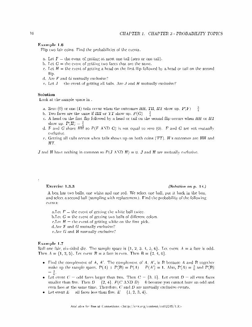
Example 1.6Flip two fair coins. Find the probabilities of the events.
a. Let F = the event of getting at most one tail (zero or one tail).b. Let G = the event of getting two faces that are the same.c. Let H = the event of getting a head on the �rst �ip followed by a head or tail on the second
�ip.d. Are F and G mutually exclusive?e. Let J = the event of getting all tails. Are J and H mutually exclusive?
SolutionLook at the sample space in .
a. Zero (0) or one (1) tails occur when the outcomes HH, TH, HT show up. P(F) = 34
b. Two faces are the same if HH or TT show up. P(G) = 24
c. A head on the �rst �ip followed by a head or tail on the second �ip occurs when HH or HTshow up. P(H) = 2
4d. F and G share HH so P(F AND G) is not equal to zero (0). F and G are not mutually
exclusive.e. Getting all tails occurs when tails shows up on both coins (TT). H 's outcomes are HH and
HT.
J and H have nothing in common so P(J AND H) = 0. J and H are mutually exclusive.
:
Exercise 1.3.3 (Solution on p. 54.)
A box has two balls, one white and one red. We select one ball, put it back in the box,and select a second ball (sampling with replacement). Find the probability of the followingevents:
a.Let F = the event of getting the white ball twice.b.Let G = the event of getting two balls of di�erent colors.c.Let H = the event of getting white on the �rst pick.d.Are F and G mutually exclusive?e.Are G and H mutually exclusive?
Example 1.7Roll one fair, six-sided die. The sample space is {1, 2, 3, 4, 5, 6}. Let event A = a face is odd.Then A = {1, 3, 5}. Let event B = a face is even. Then B = {2, 4, 6}.
• Find the complement of A, A′. The complement of A, A′, is B because A and B togethermake up the sample space. P(A) + P(B) = P(A) + P(A′) = 1. Also, P(A) = 3
6 and P(B)= 3
6 .• Let event C = odd faces larger than two. Then C = {3, 5}. Let event D = all even faces
smaller than �ve. Then D = {2, 4}. P(C AND D) = 0 because you cannot have an odd andeven face at the same time. Therefore, C and D are mutually exclusive events.
• Let event E = all faces less than �ve. E = {1, 2, 3, 4}.
Available for free at Connexions <http://cnx.org/content/col12245/1.3>
17
ProblemAre C and E mutually exclusive events? (Answer yes or no.) Why or why not?
No. C = {3, 5} and E = {1, 2, 3, 4}. P(C AND E) = 16 . To be mutually exclusive, P(C AND E)
must be zero.
• Find P(C |A). This is a conditional probability. Recall that the event C is {3, 5} and eventA is {1, 3, 5}. To �nd P(C |A), �nd the probability of C using the sample space A. You havereduced the sample space from the original sample space {1, 2, 3, 4, 5, 6} to {1, 3, 5}. So,P(C |A) = 2
3 .
:
Exercise 1.3.4 (Solution on p. 54.)
Let event A = learning Spanish. Let event B = learning German. Then A AND B =learning Spanish and German. Suppose P(A) = 0.4 and P(B) = 0.2. P(A AND B) =0.08. Are events A and B independent? Hint: You must show ONE of the following:
• P(A|B) = P(A)• P(B|A)• P(A AND B) = P(A)P(B)
Example 1.8Let event G = taking a math class. Let event H = taking a science class. Then, G AND H =taking a math class and a science class. Suppose P(G) = 0.6, P(H) = 0.5, and P(G AND H) =0.3. Are G and H independent?
If G and H are independent, then you must show ONE of the following:
• P(G|H) = P(G)• P(H |G) = P(H)• P(G AND H) = P(G)P(H)
: The choice you make depends on the information you have. You could choose any ofthe methods here because you have the necessary information.
Problem 1a. Show that P(G|H) = P(G).
SolutionP(G|H) = P (G AND H)
P (H) = 0.30.5 = 0.6 = P(G)
Problem 2b. Show P(G AND H) = P(G)P(H).
SolutionP(G)P(H) = (0.6)(0.5) = 0.3 = P(G AND H)
Available for free at Connexions <http://cnx.org/content/col12245/1.3>
18 CHAPTER 1. CHAPTER 3 - PROBABILITY TOPICS
Since G and H are independent, knowing that a person is taking a science class does not change thechance that he or she is taking a math class. If the two events had not been independent (that is,they are dependent) then knowing that a person is taking a science class would change the chancehe or she is taking math. For practice, show that P(H |G) = P(H) to show that G and H areindependent events.
:
Exercise 1.3.5 (Solution on p. 54.)
In a bag, there are six red marbles and four green marbles. The red marbles are markedwith the numbers 1, 2, 3, 4, 5, and 6. The green marbles are marked with the numbers 1,2, 3, and 4.
• R = a red marble• G = a green marble• O = an odd-numbered marble• The sample space is S = {R1, R2, R3, R4, R5, R6, G1, G2, G3, G4}.
S has ten outcomes. What is P(G AND O)?
Example 1.9Let event C = taking an English class. Let event D = taking a speech class.Suppose P(C) = 0.75, P(D) = 0.3, P(C |D) = 0.75 and P(C AND D) = 0.225.Justify your answers to the following questions numerically.
a. Are C and D independent?b. Are C and D mutually exclusive?c. What is P(D|C)?
a. Yes, because P(C |D) = P(C).b. No, because P(C AND D) is not equal to zero.
c. P(D|C) = P (C AND D)P (C) = 0.225
0.75 = 0.3
:
Exercise 1.3.6 (Solution on p. 54.)
A student goes to the library. Let events B = the student checks out a book and D =the student checks out a DVD. Suppose that P(B) = 0.40, P(D) = 0.30 and P(B ANDD) = 0.20.
a.Find P(B|D).b.Find P(D|B).c.Are B and D independent?d.Are B and D mutually exclusive?
Available for free at Connexions <http://cnx.org/content/col12245/1.3>

19
Example 1.10In a box there are three red cards and �ve blue cards. The red cards are marked with the numbers1, 2, and 3, and the blue cards are marked with the numbers 1, 2, 3, 4, and 5. The cards arewell-shu�ed. You reach into the box (you cannot see into it) and draw one card.
Let R = red card is drawn, B = blue card is drawn, E = even-numbered card is drawn.The sample space S = R1, R2, R3, B1, B2, B3, B4, B5. S has eight outcomes.
• P(R) = 38 . P(B) =
58 . P(R AND B) = 0. (You cannot draw one card that is both red and
blue.)• P(E) = 3
8 . (There are three even-numbered cards, R2, B2, and B4.)• P(E|B) = 2
5 . (There are �ve blue cards: B1, B2, B3, B4, and B5. Out of the blue cards,there are two even cards; B2 and B4.)
• P(B|E) = 23 . (There are three even-numbered cards: R2, B2, and B4. Out of the even-
numbered cards, to are blue; B2 and B4.)• The events R and B are mutually exclusive because P(R AND B) = 0.• Let G = card with a number greater than 3. G = {B4, B5}. P(G) = 2
8 . Let H = blue cardnumbered between one and four, inclusive. H = {B1, B2, B3, B4}. P(G|H) = 1
4 . (The onlycard in H that has a number greater than three is B4.) Since 2
8 = 14 , P(G) = P(G|H), which
means that G and H are independent.
:
Exercise 1.3.7 (Solution on p. 55.)
In a basketball arena,
• 70% of the fans are rooting for the home team.• 25% of the fans are wearing blue.• 20% of the fans are wearing blue and are rooting for the away team.• Of the fans rooting for the away team, 67% are wearing blue.
Let A be the event that a fan is rooting for the away team.Let B be the event that a fan is wearing blue.Are the events of rooting for the away team and wearing blue independent? Are theymutually exclusive?
Example 1.11In a particular college class, 60% of the students are female. Fifty percent of all students in theclass have long hair. Forty-�ve percent of the students are female and have long hair. Of the femalestudents, 75% have long hair. Let F be the event that a student is female. Let L be the eventthat a student has long hair. One student is picked randomly. Are the events of being female andhaving long hair independent?
• The following probabilities are given in this example:• P(F) = 0.60; P(L) = 0.50• P(F AND L) = 0.45• P(L|F) = 0.75
: The choice you make depends on the information you have. You could use the �rstor last condition on the list for this example. You do not know P(F|L) yet, so you cannot use thesecond condition.
Available for free at Connexions <http://cnx.org/content/col12245/1.3>
20 CHAPTER 1. CHAPTER 3 - PROBABILITY TOPICS
Solution 1Check whether P(F AND L) = P(F)P(L). We are given that P(F AND L) = 0.45, but P(F)P(L) =(0.60)(0.50) = 0.30. The events of being female and having long hair are not independent becauseP(F AND L) does not equal P(F)P(L).Solution 2Check whether P(L|F) equals P(L). We are given that P(L|F) = 0.75, but P(L) = 0.50; they arenot equal. The events of being female and having long hair are not independent.Interpretation of ResultsThe events of being female and having long hair are not independent; knowing that a student isfemale changes the probability that a student has long hair.
:
Exercise 1.3.8 (Solution on p. 55.)
Mark is deciding which route to take to work. His choices are I = the Interstate and F= Fifth Street.
• P(I) = 0.44 and P(F) = 0.55• P(I AND F) = 0 because Mark will take only one route to work.
What is the probability of P(I OR F)?
Example 1.12
a. Toss one fair coin (the coin has two sides, H and T). The outcomes are ________. Countthe outcomes. There are ____ outcomes.
b. Toss one fair, six-sided die (the die has 1, 2, 3, 4, 5 or 6 dots on a side). The outcomes are________________. Count the outcomes. There are ___ outcomes.
c. Multiply the two numbers of outcomes. The answer is _______.d. If you �ip one fair coin and follow it with the toss of one fair, six-sided die, the answer in
three is the number of outcomes (size of the sample space). What are the outcomes? (Hint:Two of the outcomes are H1 and T6.)
e. Event A = heads (H) on the coin followed by an even number (2, 4, 6) on the die.A = {_________________}. Find P(A).
f. Event B = heads on the coin followed by a three on the die. B = {________}. FindP(B).
g. Are A and B mutually exclusive? (Hint: What is P(A AND B)? If P(A AND B) = 0, thenA and B are mutually exclusive.)
h. Are A and B independent? (Hint: Is P(A AND B) = P(A)P(B)? If P(A AND B) =P(A)P(B), then A and B are independent. If not, then they are dependent).
a. H and T; 2b. 1, 2, 3, 4, 5, 6; 6c. 2(6) = 12d. T1, T2, T3, T4, T5, T6, H1, H2, H3, H4, H5, H6e. A = {H2, H4, H6}; P(A) = 3
12f. B = {H3}; P(B) = 1
12g. Yes, because P(A AND B) = 0h. P(A AND B) = 0.P(A)P(B) =
(312
)(112
). P(A AND B) does not equal P(A)P(B), so A and
B are dependent.
Available for free at Connexions <http://cnx.org/content/col12245/1.3>
21
:
Exercise 1.3.9 (Solution on p. 55.)
A box has two balls, one white and one red. We select one ball, put it back in the box,and select a second ball (sampling with replacement). Let T be the event of getting thewhite ball twice, F the event of picking the white ball �rst, S the event of picking thewhite ball in the second drawing.
a.Compute P(T).b.Compute P(T|F).c.Are T and F independent?.d.Are F and S mutually exclusive?e.Are F and S independent?
1.3.3 References
Lopez, Shane, Preety Sidhu. �U.S. Teachers Love Their Lives, but Struggle in the Workplace.� GallupWellbeing, 2013. http://www.gallup.com/poll/161516/teachers-love-lives-struggle-workplace.aspx (accessedMay 2, 2013).
Data from Gallup. Available online at www.gallup.com/ (accessed May 2, 2013).
1.3.4 Chapter Review
Two events A and B are independent if the knowledge that one occurred does not a�ect the chance the otheroccurs. If two events are not independent, then we say that they are dependent.
In sampling with replacement, each member of a population is replaced after it is picked, so that memberhas the possibility of being chosen more than once, and the events are considered to be independent. Insampling without replacement, each member of a population may be chosen only once, and the events areconsidered not to be independent. When events do not share outcomes, they are mutually exclusive of eachother.
1.3.5 Formula Review
If A and B are independent, P(A ∩ B) = P(A)P(B), P(A|B) = P(A) and P(B|A) = P(B).If A and B are mutually exclusive, P(A ∪ B) = P(A) + P(B) and P(A AND B) = 0.
Available for free at Connexions <http://cnx.org/content/col12245/1.3>
22 CHAPTER 1. CHAPTER 3 - PROBABILITY TOPICS
1.3.6
Exercise 1.3.10E and F are mutually exclusive events. P(E) = 0.4; P(F) = 0.5. Find P(E|F).Exercise 1.3.11 (Solution on p. 55.)
J and K are independent events. P(J|K) = 0.3. Find P(J).
Exercise 1.3.12U and V are mutually exclusive events. P(U) = 0.26; P(V ) = 0.37. Find:
a. P(U AND V ) =b. P(U |V ) =c. P(U OR V ) =
Exercise 1.3.13 (Solution on p. 55.)
Q and R are independent events. P(Q) = 0.4 and P(Q AND R) = 0.1. Find P(R).
1.3.7 Homework
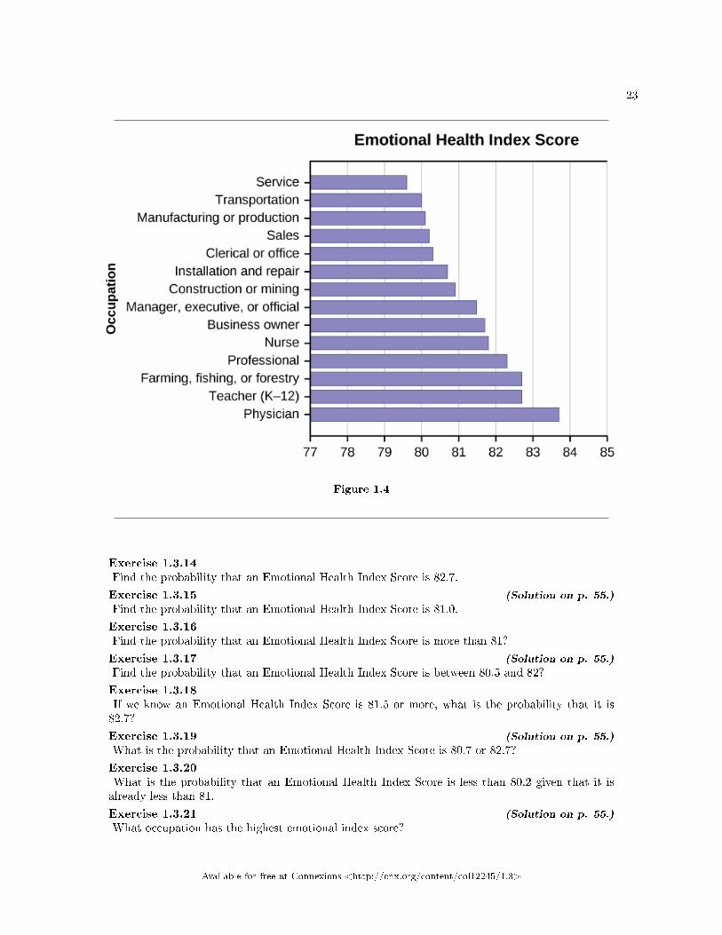
Use the following information to answer the next 12 exercises. The graph shown is based on more than170,000 interviews done by Gallup that took place from January through December 2012. The sampleconsists of employed Americans 18 years of age or older. The Emotional Health Index Scores are the samplespace. We randomly sample one Emotional Health Index Score.
Available for free at Connexions <http://cnx.org/content/col12245/1.3>
23
Figure 1.4
Exercise 1.3.14Find the probability that an Emotional Health Index Score is 82.7.
Exercise 1.3.15 (Solution on p. 55.)
Find the probability that an Emotional Health Index Score is 81.0.
Exercise 1.3.16Find the probability that an Emotional Health Index Score is more than 81?
Exercise 1.3.17 (Solution on p. 55.)
Find the probability that an Emotional Health Index Score is between 80.5 and 82?
Exercise 1.3.18If we know an Emotional Health Index Score is 81.5 or more, what is the probability that it is82.7?
Exercise 1.3.19 (Solution on p. 55.)
What is the probability that an Emotional Health Index Score is 80.7 or 82.7?
Exercise 1.3.20What is the probability that an Emotional Health Index Score is less than 80.2 given that it isalready less than 81.
Exercise 1.3.21 (Solution on p. 55.)
What occupation has the highest emotional index score?
Available for free at Connexions <http://cnx.org/content/col12245/1.3>
24 CHAPTER 1. CHAPTER 3 - PROBABILITY TOPICS
Exercise 1.3.22What occupation has the lowest emotional index score?
Exercise 1.3.23 (Solution on p. 55.)
What is the range of the data?
Exercise 1.3.24Compute the average EHIS.
Exercise 1.3.25 (Solution on p. 55.)
If all occupations are equally likely for a certain individual, what is the probability that he or shewill have an occupation with lower than average EHIS?
1.3.8 Bringing It Together
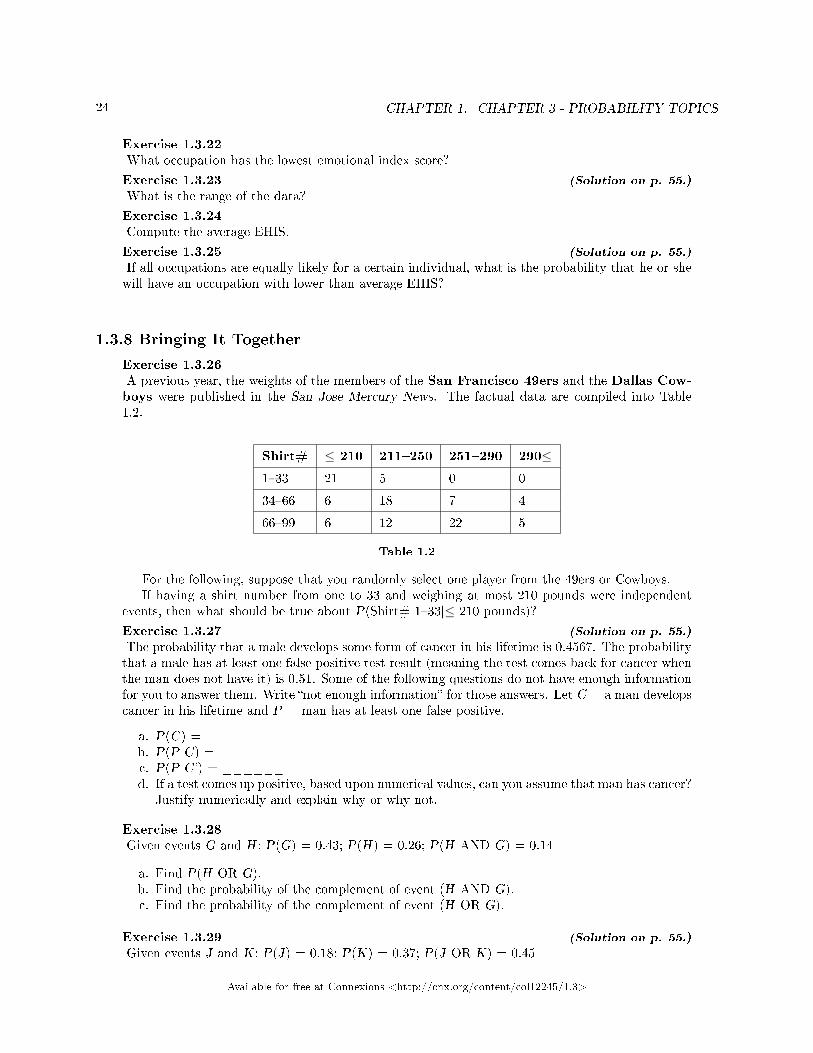
Exercise 1.3.26A previous year, the weights of the members of the San Francisco 49ers and the Dallas Cow-boys were published in the San Jose Mercury News. The factual data are compiled into Table1.2.
Shirt# ≤ 210 211�250 251�290 290≤1�33 21 5 0 0
34�66 6 18 7 4
66�99 6 12 22 5
Table 1.2
For the following, suppose that you randomly select one player from the 49ers or Cowboys.If having a shirt number from one to 33 and weighing at most 210 pounds were independent
events, then what should be true about P(Shirt# 1�33|≤ 210 pounds)?
Exercise 1.3.27 (Solution on p. 55.)
The probability that a male develops some form of cancer in his lifetime is 0.4567. The probabilitythat a male has at least one false positive test result (meaning the test comes back for cancer whenthe man does not have it) is 0.51. Some of the following questions do not have enough informationfor you to answer them. Write �not enough information� for those answers. Let C = a man developscancer in his lifetime and P = man has at least one false positive.
a. P(C) = ______b. P(P|C) = ______c. P(P|C') = ______d. If a test comes up positive, based upon numerical values, can you assume that man has cancer?
Justify numerically and explain why or why not.
Exercise 1.3.28Given events G and H : P(G) = 0.43; P(H) = 0.26; P(H AND G) = 0.14
a. Find P(H OR G).b. Find the probability of the complement of event (H AND G).c. Find the probability of the complement of event (H OR G).
Exercise 1.3.29 (Solution on p. 55.)
Given events J and K : P(J) = 0.18; P(K) = 0.37; P(J OR K) = 0.45
Available for free at Connexions <http://cnx.org/content/col12245/1.3>
25
a. Find P(J AND K).b. Find the probability of the complement of event (J AND K).c. Find the probability of the complement of event (J AND K).
1.4 Two Basic Rules of Probability4
When calculating probability, there are two rules to consider when determining if two events are independentor dependent and if they are mutually exclusive or not.
1.4.1 The Multiplication Rule
If A and B are two events de�ned on a sample space, then: P (A ∩B) = P (B)P (A|B). We can think ofthe intersection symbol as substituting for the word "and".
This rule may also be written as: P (A|B) = P (A∩B)P (B)
This equation is read as the probability of A given B equals the probability of A and B divided by theprobability of B.
If A and B are independent, then P (A|B) = P (A). Then P (A ∩B) = P (A|B)P (B) becomesP (A ∩B) = P (A) (B) because the P (A|B) = P (A) if A and B are independent.
One easy way to remember the multiplication rule is that the word "and" means that the event has tosatisfy two conditions. For example the name drawn from the class roster is to be both a female and asophomore. It is harder to satisfy two conditions than only one and of course when we multiply fractionsthe result is always smaller. This re�ects the increasing di�culty of satisfying two conditions.
1.4.2 The Addition Rule
If A and B are de�ned on a sample space, then: P (A ∪B) = P (A) + P (B)− P (A ∩B). We can think ofthe union symbol substituting for the word "or". The reason we subtract the intersection of A and B is tokeep from double counting elements that are in both A and B.
If A and B are mutually exclusive, then P (A ∩B) = 0. Then P (A ∪B) = P (A)+P (B)−P (A ∩B)becomes P (A ∪B) = P (A) + P (B).
Example 1.13Klaus is trying to choose where to go on vacation. His two choices are: A = New Zealand and B= Alaska
• Klaus can only a�ord one vacation. The probability that he chooses A is P(A) = 0.6 and theprobability that he chooses B is P(B) = 0.35.
• P (A ∩B) = 0 because Klaus can only a�ord to take one vacation• Therefore, the probability that he chooses either New Zealand or Alaska is P (A ∪B) =
P (A) + P (B) = 0.6 + 0.35 = 0.95. Note that the probability that he does not choose to goanywhere on vacation must be 0.05.
Example 1.14Carlos plays college soccer. He makes a goal 65% of the time he shoots. Carlos is going to attempttwo goals in a row in the next game. A = the event Carlos is successful on his �rst attempt. P(A)= 0.65. B = the event Carlos is successful on his second attempt. P(B) = 0.65. Carlos tends toshoot in streaks. The probability that he makes the second goal | that he made the �rst goal is 0.90.
4This content is available online at <http://cnx.org/content/m54220/1.14/>.
Available for free at Connexions <http://cnx.org/content/col12245/1.3>
26 CHAPTER 1. CHAPTER 3 - PROBABILITY TOPICS
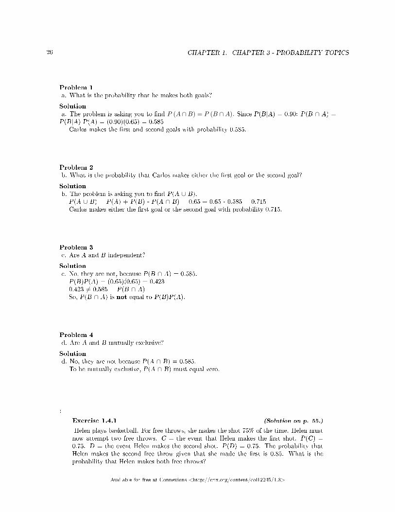
Problem 1a. What is the probability that he makes both goals?
Solutiona. The problem is asking you to �nd P (A ∩B) = P (B ∩A). Since P(B|A) = 0.90: P(B ∩ A) =P(B|A) P(A) = (0.90)(0.65) = 0.585
Carlos makes the �rst and second goals with probability 0.585.
Problem 2b. What is the probability that Carlos makes either the �rst goal or the second goal?
Solutionb. The problem is asking you to �nd P(A ∪ B).
P(A ∪ B) = P(A) + P(B) - P(A ∩ B) = 0.65 + 0.65 - 0.585 = 0.715Carlos makes either the �rst goal or the second goal with probability 0.715.
Problem 3c. Are A and B independent?
Solutionc. No, they are not, because P(B ∩ A) = 0.585.
P(B)P(A) = (0.65)(0.65) = 0.4230.423 6= 0.585 = P(B ∩ A)So, P(B ∩ A) is not equal to P(B)P(A).
Problem 4d. Are A and B mutually exclusive?
Solutiond. No, they are not because P(A ∩ B) = 0.585.
To be mutually exclusive, P(A ∩ B) must equal zero.
:
Exercise 1.4.1 (Solution on p. 55.)
Helen plays basketball. For free throws, she makes the shot 75% of the time. Helen mustnow attempt two free throws. C = the event that Helen makes the �rst shot. P(C) =0.75. D = the event Helen makes the second shot. P(D) = 0.75. The probability thatHelen makes the second free throw given that she made the �rst is 0.85. What is theprobability that Helen makes both free throws?
Available for free at Connexions <http://cnx.org/content/col12245/1.3>
27
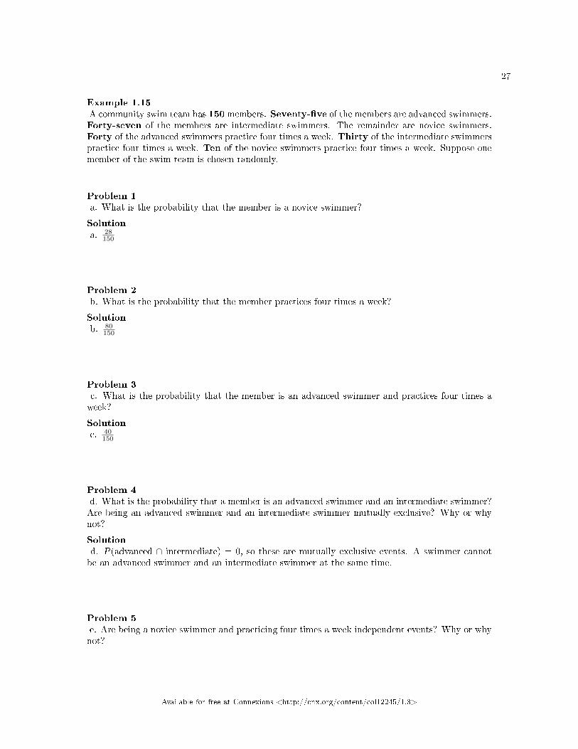
Example 1.15A community swim team has 150members. Seventy-�ve of the members are advanced swimmers.Forty-seven of the members are intermediate swimmers. The remainder are novice swimmers.Forty of the advanced swimmers practice four times a week. Thirty of the intermediate swimmerspractice four times a week. Ten of the novice swimmers practice four times a week. Suppose onemember of the swim team is chosen randomly.
Problem 1a. What is the probability that the member is a novice swimmer?
Solutiona. 28
150
Problem 2b. What is the probability that the member practices four times a week?
Solutionb. 80
150
Problem 3c. What is the probability that the member is an advanced swimmer and practices four times aweek?
Solutionc. 40
150
Problem 4d. What is the probability that a member is an advanced swimmer and an intermediate swimmer?Are being an advanced swimmer and an intermediate swimmer mutually exclusive? Why or whynot?
Solutiond. P(advanced ∩ intermediate) = 0, so these are mutually exclusive events. A swimmer cannotbe an advanced swimmer and an intermediate swimmer at the same time.
Problem 5e. Are being a novice swimmer and practicing four times a week independent events? Why or whynot?
Available for free at Connexions <http://cnx.org/content/col12245/1.3>

28 CHAPTER 1. CHAPTER 3 - PROBABILITY TOPICS
Solutione. No, these are not independent events.P(novice ∩ practices four times per week) = 0.0667P(novice)P(practices four times per week) = 0.09960.0667 6= 0.0996
:
Exercise 1.4.2 (Solution on p. 55.)
A school has 200 seniors of whom 140 will be going to college next year. Forty will begoing directly to work. The remainder are taking a gap year. Fifty of the seniors going tocollege play sports. Thirty of the seniors going directly to work play sports. Five of theseniors taking a gap year play sports. What is the probability that a senior is taking agap year?
Example 1.16Felicity attends Modesto JC in Modesto, CA. The probability that Felicity enrolls in a math classis 0.2 and the probability that she enrolls in a speech class is 0.65. The probability that she enrollsin a math class | that she enrolls in speech class is 0.25.
Let: M = math class, S = speech class, M |S = math given speech
Problem
a. What is the probability that Felicity enrolls in math and speech?Find P(M ∩ S) = P(M |S)P(S).
b. What is the probability that Felicity enrolls in math or speech classes?Find P(M ∪ S) = P(M) + P(S) - P(M ∩ S).
c. Are M and S independent? Is P(M |S) = P(M)?d. Are M and S mutually exclusive? Is P(M ∩ S) = 0?
Solutiona. 0.1625, b. 0.6875, c. No, d. No
:
Exercise 1.4.3 (Solution on p. 56.)
A student goes to the library. Let events B = the student checks out a book and D = thestudent check out a DVD. Suppose that P(B) = 0.40, P(D) = 0.30 and P(D|B) = 0.5.
a.Find P(B ∩ D).b.Find P(B ∪ D).
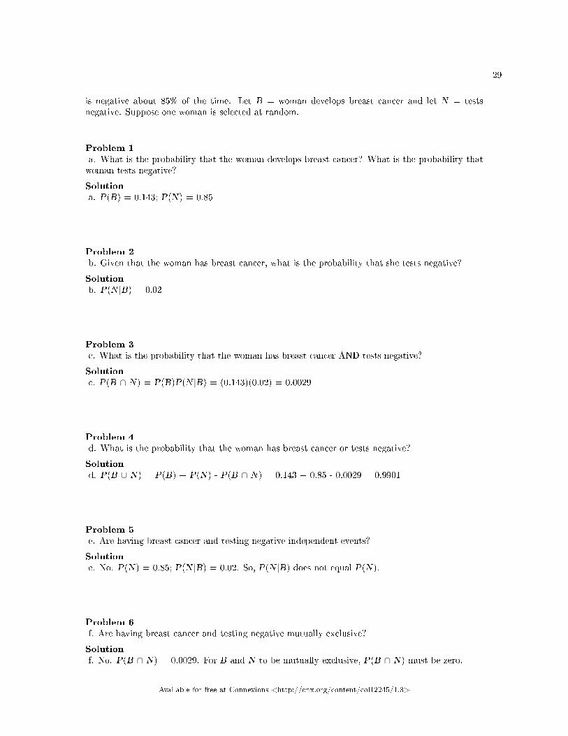
Example 1.17Studies show that about one woman in seven (approximately 14.3%) who live to be 90 will developbreast cancer. Suppose that of those women who develop breast cancer, a test is negative 2%of the time. Also suppose that in the general population of women, the test for breast cancer
Available for free at Connexions <http://cnx.org/content/col12245/1.3>
29
is negative about 85% of the time. Let B = woman develops breast cancer and let N = testsnegative. Suppose one woman is selected at random.
Problem 1a. What is the probability that the woman develops breast cancer? What is the probability thatwoman tests negative?
Solutiona. P(B) = 0.143; P(N) = 0.85
Problem 2b. Given that the woman has breast cancer, what is the probability that she tests negative?
Solutionb. P(N |B) = 0.02
Problem 3c. What is the probability that the woman has breast cancer AND tests negative?
Solutionc. P(B ∩ N) = P(B)P(N |B) = (0.143)(0.02) = 0.0029
Problem 4d. What is the probability that the woman has breast cancer or tests negative?
Solutiond. P(B ∪ N) = P(B) + P(N) - P(B ∩ N) = 0.143 + 0.85 - 0.0029 = 0.9901
Problem 5e. Are having breast cancer and testing negative independent events?
Solutione. No. P(N) = 0.85; P(N |B) = 0.02. So, P(N |B) does not equal P(N).
Problem 6f. Are having breast cancer and testing negative mutually exclusive?
Solutionf. No. P(B ∩ N) = 0.0029. For B and N to be mutually exclusive, P(B ∩ N) must be zero.
Available for free at Connexions <http://cnx.org/content/col12245/1.3>

30 CHAPTER 1. CHAPTER 3 - PROBABILITY TOPICS
:
Exercise 1.4.4 (Solution on p. 56.)
A school has 200 seniors of whom 140 will be going to college next year. Forty will begoing directly to work. The remainder are taking a gap year. Fifty of the seniors going tocollege play sports. Thirty of the seniors going directly to work play sports. Five of theseniors taking a gap year play sports. What is the probability that a senior is going tocollege and plays sports?
Example 1.18Refer to the information in Example 1.17. P = tests positive.
a. Given that a woman develops breast cancer, what is the probability that she tests positive.Find P(P|B) = 1 - P(N |B).
b. What is the probability that a woman develops breast cancer and tests positive. Find P(B ∩P) = P(P|B)P(B).
c. What is the probability that a woman does not develop breast cancer. Find P(B′) = 1 -P(B).
d. What is the probability that a woman tests positive for breast cancer. Find P(P) = 1 - P(N).
Solutiona. 0.98; b. 0.1401; c. 0.857; d. 0.15
:
Exercise 1.4.5 (Solution on p. 56.)
A student goes to the library. Let events B = the student checks out a book and D = thestudent checks out a DVD. Suppose that P(B) = 0.40, P(D) = 0.30 and P(D|B) = 0.5.
a.Find P(B′).b.Find P(D ∩ B).c.Find P(B|D).d.Find P(D ∩ B′).e.Find P(D|B′).
1.4.3 References
DiCamillo, Mark, Mervin Field. �The File Poll.� Field Research Corporation. Available online athttp://www.�eld.com/�eldpollonline/subscribers/Rls2443.pdf (accessed May 2, 2013).
Rider, David, �Ford support plummeting, poll suggests,� The Star, September 14, 2011. Available on-line at http://www.thestar.com/news/gta/2011/09/14/ford_support_plummeting_poll_suggests.html (ac-cessed May 2, 2013).
Available for free at Connexions <http://cnx.org/content/col12245/1.3>
31
�Mayor's Approval Down.� News Release by Forum Research Inc. Available onlineat http://www.forumresearch.com/forms/News Archives/News Releases/74209_TO_Issues_-_Mayoral_Approval_%28Forum_Research%29%2820130320%29.pdf (accessed May 2, 2013).
�Roulette.� Wikipedia. Available online at http://en.wikipedia.org/wiki/Roulette (accessed May 2,2013).
Shin, Hyon B., Robert A. Kominski. �Language Use in the United States: 2007.� United States Cen-sus Bureau. Available online at http://www.census.gov/hhes/socdemo/language/data/acs/ACS-12.pdf (ac-cessed May 2, 2013).
Data from the Baseball-Almanac, 2013. Available online at www.baseball-almanac.com (accessed May 2,2013).
Data from U.S. Census Bureau.Data from the Wall Street Journal.Data from The Roper Center: Public Opinion Archives at the University of Connecticut. Available online
at http://www.ropercenter.uconn.edu/ (accessed May 2, 2013).Data from Field Research Corporation. Available online at www.�eld.com/�eldpollonline (accessed May
2,2 013).
1.4.4 Chapter Review
The multiplication rule and the addition rule are used for computing the probability of A and B, as wellas the probability of A or B for two given events A, B de�ned on the sample space. In sampling withreplacement each member of a population is replaced after it is picked, so that member has the possibilityof being chosen more than once, and the events are considered to be independent. In sampling withoutreplacement, each member of a population may be chosen only once, and the events are considered to benot independent. The events A and B are mutually exclusive events when they do not have any outcomesin common.
1.4.5 Formula Review
The multiplication rule: P(A ∩ B) = P(A|B)P(B)The addition rule: P(A ∪ B) = P(A) + P(B) - P(A ∩ B)
Available for free at Connexions <http://cnx.org/content/col12245/1.3>
32 CHAPTER 1. CHAPTER 3 - PROBABILITY TOPICS
1.4.6
Use the following information to answer the next ten exercises. Forty-eight percent of all Californiansregistered voters prefer life in prison without parole over the death penalty for a person convicted of �rstdegree murder. Among Latino California registered voters, 55% prefer life in prison without parole over thedeath penalty for a person convicted of �rst degree murder. 37.6% of all Californians are Latino.
In this problem, let:
• C = Californians (registered voters) preferring life in prison without parole over the death penalty fora person convicted of �rst degree murder.
• L = Latino Californians
Suppose that one Californian is randomly selected.
Exercise 1.4.6Find P(C).
Exercise 1.4.7 (Solution on p. 56.)
Find P(L).
Exercise 1.4.8Find P(C |L).Exercise 1.4.9 (Solution on p. 56.)
In words, what is C |L?Exercise 1.4.10Find P(L ∩ C).
Exercise 1.4.11 (Solution on p. 56.)
In words, what is L ∩ C?
Exercise 1.4.12Are L and C independent events? Show why or why not.
Exercise 1.4.13 (Solution on p. 56.)
Find P(L ∪ C).
Exercise 1.4.14In words, what is L ∪ C?
Exercise 1.4.15 (Solution on p. 56.)
Are L and C mutually exclusive events? Show why or why not.
1.4.7 Homework
Exercise 1.4.16On February 28, 2013, a Field Poll Survey reported that 61% of California registered voters approvedof allowing two people of the same gender to marry and have regular marriage laws apply tothem. Among 18 to 39 year olds (California registered voters), the approval rating was 78%.Six in ten California registered voters said that the upcoming Supreme Court's ruling about theconstitutionality of California's Proposition 8 was either very or somewhat important to them. Outof those CA registered voters who support same-sex marriage, 75% say the ruling is important tothem.
In this problem, let:
• C = California registered voters who support same-sex marriage.• B = California registered voters who say the Supreme Court's ruling about the constitution-
ality of California's Proposition 8 is very or somewhat important to them
Available for free at Connexions <http://cnx.org/content/col12245/1.3>
33
• A = California registered voters who are 18 to 39 years old.
a. Find P(C).b. Find P(B).c. Find P(C |A).d. Find P(B|C).e. In words, what is C |A?f. In words, what is B|C?g. Find P(C ∩ B).h. In words, what is C ∩ B?i. Find P(C ∪ B).j. Are C and B mutually exclusive events? Show why or why not.
Exercise 1.4.17 (Solution on p. 56.)
After Rob Ford, the mayor of Toronto, announced his plans to cut budget costs in late 2011, theForum Research polled 1,046 people to measure the mayor's popularity. Everyone polled expressedeither approval or disapproval. These are the results their poll produced:
• In early 2011, 60 percent of the population approved of Mayor Ford's actions in o�ce.• In mid-2011, 57 percent of the population approved of his actions.• In late 2011, the percentage of popular approval was measured at 42 percent.
a. What is the sample size for this study?b. What proportion in the poll disapproved of Mayor Ford, according to the results from late
2011?c. How many people polled responded that they approved of Mayor Ford in late 2011?d. What is the probability that a person supported Mayor Ford, based on the data collected in
mid-2011?e. What is the probability that a person supported Mayor Ford, based on the data collected in
early 2011?
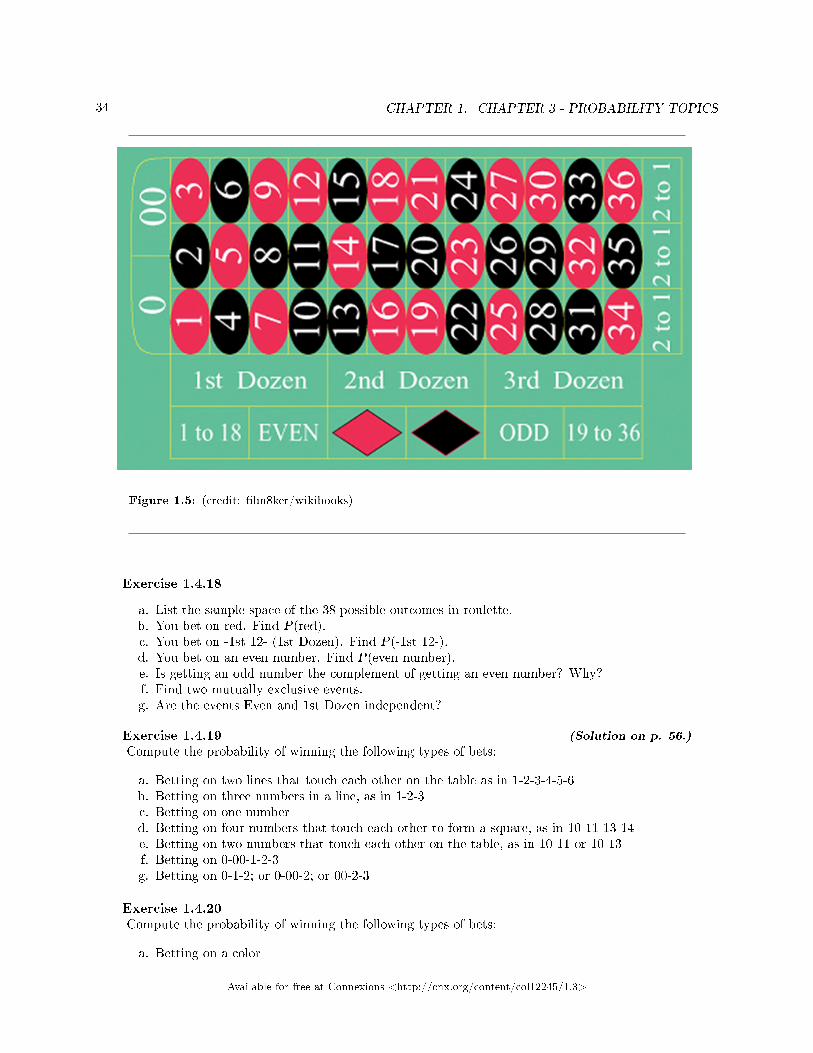
Use the following information to answer the next three exercises. The casino game, roulette, allows thegambler to bet on the probability of a ball, which spins in the roulette wheel, landing on a particular color,number, or range of numbers. The table used to place bets contains of 38 numbers, and each number isassigned to a color and a range.
Available for free at Connexions <http://cnx.org/content/col12245/1.3>
34 CHAPTER 1. CHAPTER 3 - PROBABILITY TOPICS
Figure 1.5: (credit: �lm8ker/wikibooks)
Exercise 1.4.18
a. List the sample space of the 38 possible outcomes in roulette.b. You bet on red. Find P(red).c. You bet on -1st 12- (1st Dozen). Find P(-1st 12-).d. You bet on an even number. Find P(even number).e. Is getting an odd number the complement of getting an even number? Why?f. Find two mutually exclusive events.g. Are the events Even and 1st Dozen independent?
Exercise 1.4.19 (Solution on p. 56.)
Compute the probability of winning the following types of bets:
a. Betting on two lines that touch each other on the table as in 1-2-3-4-5-6b. Betting on three numbers in a line, as in 1-2-3c. Betting on one numberd. Betting on four numbers that touch each other to form a square, as in 10-11-13-14e. Betting on two numbers that touch each other on the table, as in 10-11 or 10-13f. Betting on 0-00-1-2-3g. Betting on 0-1-2; or 0-00-2; or 00-2-3
Exercise 1.4.20Compute the probability of winning the following types of bets:
a. Betting on a color
Available for free at Connexions <http://cnx.org/content/col12245/1.3>
35
b. Betting on one of the dozen groupsc. Betting on the range of numbers from 1 to 18d. Betting on the range of numbers 19�36e. Betting on one of the columnsf. Betting on an even or odd number (excluding zero)
Exercise 1.4.21 (Solution on p. 56.)
Suppose that you have eight cards. Five are green and three are yellow. The �ve green cards arenumbered 1, 2, 3, 4, and 5. The three yellow cards are numbered 1, 2, and 3. The cards are wellshu�ed. You randomly draw one card.
• G = card drawn is green• E = card drawn is even-numbered
a. List the sample space.b. P(G) = _____c. P(G|E) = _____d. P(G ∩ E) = _____e. P(G ∪ E) = _____f. Are G and E mutually exclusive? Justify your answer numerically.
Exercise 1.4.22Roll two fair dice separately. Each die has six faces.
a. List the sample space.b. Let A be the event that either a three or four is rolled �rst, followed by an even number. Find
P(A).c. Let B be the event that the sum of the two rolls is at most seven. Find P(B).d. In words, explain what �P(A|B)� represents. Find P(A|B).e. Are A and B mutually exclusive events? Explain your answer in one to three complete
sentences, including numerical justi�cation.f. Are A and B independent events? Explain your answer in one to three complete sentences,including numerical justi�cation.
Exercise 1.4.23 (Solution on p. 57.)
A special deck of cards has ten cards. Four are green, three are blue, and three are red. When acard is picked, its color of it is recorded. An experiment consists of �rst picking a card and thentossing a coin.
a. List the sample space.b. Let A be the event that a blue card is picked �rst, followed by landing a head on the coin
toss. Find P(A).c. Let B be the event that a red or green is picked, followed by landing a head on the coin toss.
Are the events A and B mutually exclusive? Explain your answer in one to three completesentences, including numerical justi�cation.
d. Let C be the event that a red or blue is picked, followed by landing a head on the coin toss.Are the events A and C mutually exclusive? Explain your answer in one to three completesentences, including numerical justi�cation.
Exercise 1.4.24An experiment consists of �rst rolling a die and then tossing a coin.
a. List the sample space.
Available for free at Connexions <http://cnx.org/content/col12245/1.3>
36 CHAPTER 1. CHAPTER 3 - PROBABILITY TOPICS
b. Let A be the event that either a three or a four is rolled �rst, followed by landing a head onthe coin toss. Find P(A).
c. Let B be the event that the �rst and second tosses land on heads. Are the events A andB mutually exclusive? Explain your answer in one to three complete sentences, includingnumerical justi�cation.
Exercise 1.4.25 (Solution on p. 57.)
An experiment consists of tossing a nickel, a dime, and a quarter. Of interest is the side the coinlands on.
a. List the sample space.b. Let A be the event that there are at least two tails. Find P(A).c. Let B be the event that the �rst and second tosses land on heads. Are the events A and
B mutually exclusive? Explain your answer in one to three complete sentences, includingjusti�cation.
Exercise 1.4.26Consider the following scenario:Let P(C) = 0.4.Let P(D) = 0.5.Let P(C |D) = 0.6.
a. Find P(C ∩ D).b. Are C and D mutually exclusive? Why or why not?c. Are C and D independent events? Why or why not?d. Find P(C ∪ D).e. Find P(D|C).
Exercise 1.4.27 (Solution on p. 57.)
Y and Z are independent events.
a. Rewrite the basic Addition Rule P(Y ∪ Z) = P(Y ) + P(Z) - P(Y ∩ Z) using the informationthat Y and Z are independent events.
b. Use the rewritten rule to �nd P(Z) if P(Y ∪ Z) = 0.71 and P(Y ) = 0.42.
Exercise 1.4.28G and H are mutually exclusive events. P(G) = 0.5 P(H) = 0.3
a. Explain why the following statement MUST be false: P(H |G) = 0.4.b. Find P(H ∪ G).c. Are G and H independent or dependent events? Explain in a complete sentence.
Exercise 1.4.29 (Solution on p. 57.)
Approximately 281,000,000 people over age �ve live in the United States. Of these people,55,000,000 speak a language other than English at home. Of those who speak another language athome, 62.3% speak Spanish.
Let: E = speaks English at home; E′ = speaks another language at home; S = speaks Spanish;Finish each probability statement by matching the correct answer.
Available for free at Connexions <http://cnx.org/content/col12245/1.3>
37
Probability Statements Answers
a. P(E′) = i. 0.8043
b. P(E) = ii. 0.623
c. P(S ∩ E′) = iii. 0.1957
d. P(S|E′) = iv. 0.1219
Table 1.3
Exercise 1.4.301994, the U.S. government held a lottery to issue 55,000 Green Cards (permits for non-citizens towork legally in the U.S.). Renate Deutsch, from Germany, was one of approximately 6.5 millionpeople who entered this lottery. Let G = won green card.
a. What was Renate's chance of winning a Green Card? Write your answer as a probabilitystatement.
b. In the summer of 1994, Renate received a letter stating she was one of 110,000 �nalists chosen.Once the �nalists were chosen, assuming that each �nalist had an equal chance to win, whatwas Renate's chance of winning a Green Card? Write your answer as a conditional probabilitystatement. Let F = was a �nalist.
c. Are G and F independent or dependent events? Justify your answer numerically and alsoexplain why.
d. Are G and F mutually exclusive events? Justify your answer numerically and explain why.
Exercise 1.4.31 (Solution on p. 57.)
Three professors at George Washington University did an experiment to determine if economistsare more sel�sh than other people. They dropped 64 stamped, addressed envelopes with $10 cashin di�erent classrooms on the George Washington campus. 44% were returned overall. From theeconomics classes 56% of the envelopes were returned. From the business, psychology, and historyclasses 31% were returned.
Let: R = money returned; E = economics classes; O = other classes
a. Write a probability statement for the overall percent of money returned.b. Write a probability statement for the percent of money returned out of the economics classes.c. Write a probability statement for the percent of money returned out of the other classes.d. Is money being returned independent of the class? Justify your answer numerically and
explain it.e. Based upon this study, do you think that economists are more sel�sh than other people?
Explain why or why not. Include numbers to justify your answer.
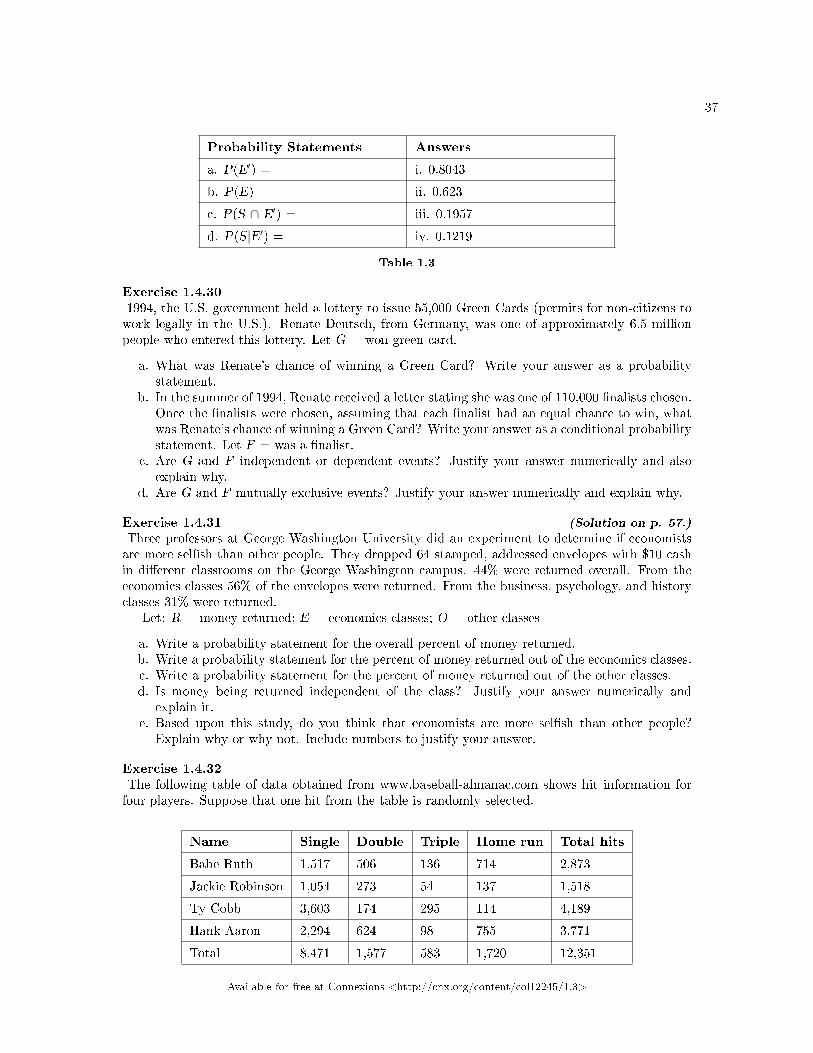
Exercise 1.4.32The following table of data obtained from www.baseball-almanac.com shows hit information forfour players. Suppose that one hit from the table is randomly selected.
Name Single Double Triple Home run Total hits
Babe Ruth 1,517 506 136 714 2,873
Jackie Robinson 1,054 273 54 137 1,518
Ty Cobb 3,603 174 295 114 4,189
Hank Aaron 2,294 624 98 755 3,771
Total 8,471 1,577 583 1,720 12,351
Available for free at Connexions <http://cnx.org/content/col12245/1.3>
38 CHAPTER 1. CHAPTER 3 - PROBABILITY TOPICS
Table 1.4
Are "the hit being made by Hank Aaron" and "the hit being a double" independent events?
a. Yes, because P(hit by Hank Aaron|hit is a double) = P(hit by Hank Aaron)b. No, because P(hit by Hank Aaron|hit is a double) 6= P(hit is a double)c. No, because P(hit is by Hank Aaron|hit is a double) 6= P(hit by Hank Aaron)d. Yes, because P(hit is by Hank Aaron|hit is a double) = P(hit is a double)
Exercise 1.4.33 (Solution on p. 57.)
United Blood Services is a blood bank that serves more than 500 hospitals in 18 states. Accordingto their website, a person with type O blood and a negative Rh factor (Rh-) can donate blood toany person with any bloodtype. Their data show that 43% of people have type O blood and 15%of people have Rh- factor; 52% of people have type O or Rh- factor.
a. Find the probability that a person has both type O blood and the Rh- factor.b. Find the probability that a person does NOT have both type O blood and the Rh- factor.
Exercise 1.4.34At a college, 72% of courses have �nal exams and 46% of courses require research papers. Supposethat 32% of courses have a research paper and a �nal exam. Let F be the event that a course hasa �nal exam. Let R be the event that a course requires a research paper.
a. Find the probability that a course has a �nal exam or a research project.b. Find the probability that a course has NEITHER of these two requirements.
Exercise 1.4.35 (Solution on p. 57.)
In a box of assorted cookies, 36% contain chocolate and 12% contain nuts. In the box, 8% containboth chocolate and nuts. Sean is allergic to both chocolate and nuts.
a. Find the probability that a cookie contains chocolate or nuts (he can't eat it).b. Find the probability that a cookie does not contain chocolate or nuts (he can eat it).
Exercise 1.4.36A college �nds that 10% of students have taken a distance learning class and that 40% of studentsare part time students. Of the part time students, 20% have taken a distance learning class. Let D= event that a student takes a distance learning class and E = event that a student is a part timestudent
a. Find P(D ∩ E).b. Find P(E|D).c. Find P(D ∪ E).d. Using an appropriate test, show whether D and E are independent.e. Using an appropriate test, show whether D and E are mutually exclusive.
Available for free at Connexions <http://cnx.org/content/col12245/1.3>
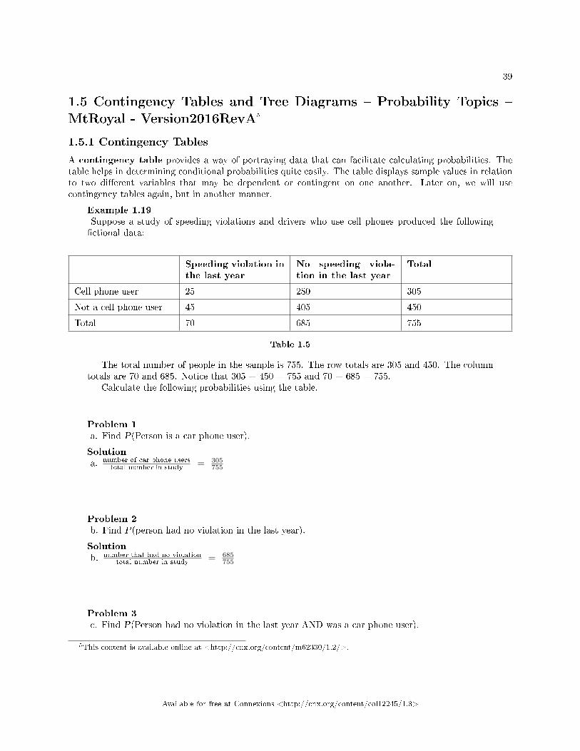
39
1.5 Contingency Tables and Tree Diagrams � Probability Topics �MtRoyal - Version2016RevA5
1.5.1 Contingency Tables
A contingency table provides a way of portraying data that can facilitate calculating probabilities. Thetable helps in determining conditional probabilities quite easily. The table displays sample values in relationto two di�erent variables that may be dependent or contingent on one another. Later on, we will usecontingency tables again, but in another manner.
Example 1.19Suppose a study of speeding violations and drivers who use cell phones produced the following�ctional data:
Speeding violation inthe last year
No speeding viola-tion in the last year
Total
Cell phone user 25 280 305
Not a cell phone user 45 405 450
Total 70 685 755
Table 1.5
The total number of people in the sample is 755. The row totals are 305 and 450. The columntotals are 70 and 685. Notice that 305 + 450 = 755 and 70 + 685 = 755.
Calculate the following probabilities using the table.
Problem 1a. Find P(Person is a car phone user).
Solutiona. number of car phone users
total number in study = 305755
Problem 2b. Find P(person had no violation in the last year).
Solutionb. number that had no violation
total number in study = 685755
Problem 3c. Find P(Person had no violation in the last year AND was a car phone user).
5This content is available online at <http://cnx.org/content/m62330/1.2/>.
Available for free at Connexions <http://cnx.org/content/col12245/1.3>
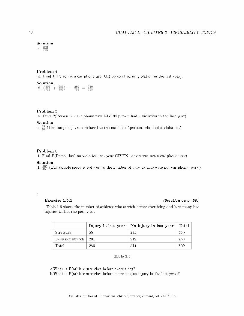
40 CHAPTER 1. CHAPTER 3 - PROBABILITY TOPICS
Solutionc. 280
755
Problem 4d. Find P(Person is a car phone user OR person had no violation in the last year).
Solutiond.(305755 + 685
755
)− 280
755 = 710755
Problem 5e. Find P(Person is a car phone user GIVEN person had a violation in the last year).
Solutione. 25
70 (The sample space is reduced to the number of persons who had a violation.)
Problem 6f. Find P(Person had no violation last year GIVEN person was not a car phone user)
Solutionf. 405
450 (The sample space is reduced to the number of persons who were not car phone users.)
:
Exercise 1.5.1 (Solution on p. 58.)
Table 1.6 shows the number of athletes who stretch before exercising and how many hadinjuries within the past year.
Injury in last year No injury in last year Total
Stretches 55 295 350
Does not stretch 231 219 450
Total 286 514 800
Table 1.6
a.What is P(athlete stretches before exercising)?b.What is P(athlete stretches before exercising|no injury in the last year)?
Available for free at Connexions <http://cnx.org/content/col12245/1.3>
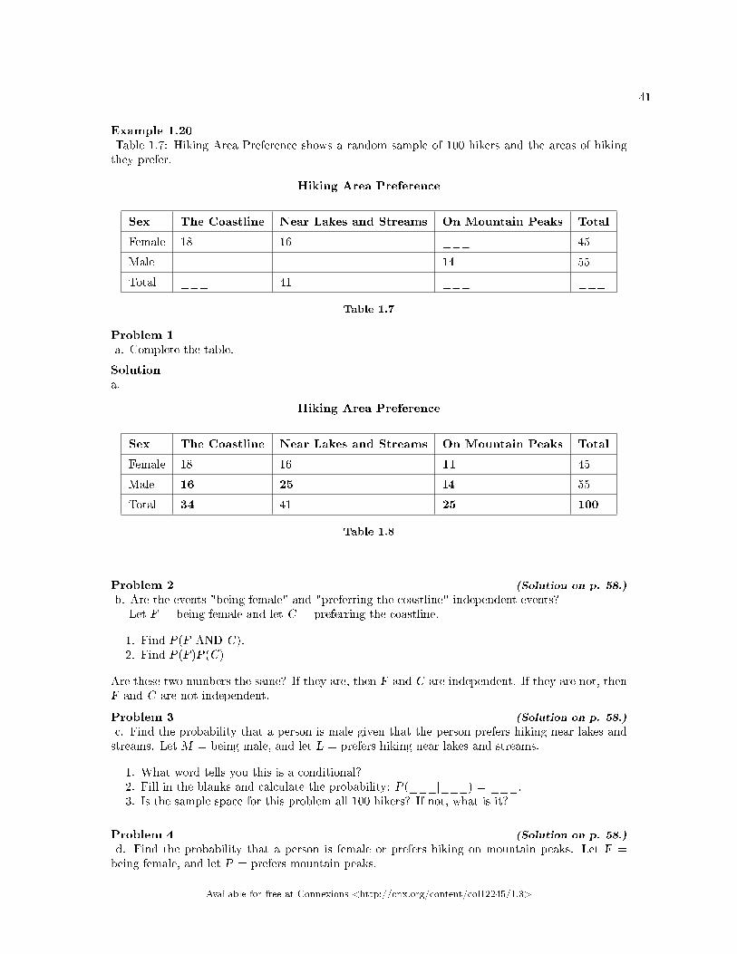
41
Example 1.20Table 1.7: Hiking Area Preference shows a random sample of 100 hikers and the areas of hikingthey prefer.
Hiking Area Preference
Sex The Coastline Near Lakes and Streams On Mountain Peaks Total
Female 18 16 ___ 45
Male ___ ___ 14 55
Total ___ 41 ___ ___
Table 1.7
Problem 1a. Complete the table.
Solutiona.
Hiking Area Preference
Sex The Coastline Near Lakes and Streams On Mountain Peaks Total
Female 18 16 11 45
Male 16 25 14 55
Total 34 41 25 100
Table 1.8
Problem 2 (Solution on p. 58.)
b. Are the events "being female" and "preferring the coastline" independent events?Let F = being female and let C = preferring the coastline.
1. Find P(F AND C).2. Find P(F)P(C)
Are these two numbers the same? If they are, then F and C are independent. If they are not, thenF and C are not independent.
Problem 3 (Solution on p. 58.)
c. Find the probability that a person is male given that the person prefers hiking near lakes andstreams. Let M = being male, and let L = prefers hiking near lakes and streams.
1. What word tells you this is a conditional?2. Fill in the blanks and calculate the probability: P(___|___) = ___.3. Is the sample space for this problem all 100 hikers? If not, what is it?
Problem 4 (Solution on p. 58.)
d. Find the probability that a person is female or prefers hiking on mountain peaks. Let F =being female, and let P = prefers mountain peaks.
Available for free at Connexions <http://cnx.org/content/col12245/1.3>

42 CHAPTER 1. CHAPTER 3 - PROBABILITY TOPICS
1. Find P(F).2. Find P(P).3. Find P(F AND P).4. Find P(F OR P).
:
Exercise 1.5.2 (Solution on p. 58.)
Table 1.9 shows a random sample of 200 cyclists and the routes they prefer. Let M =males and H = hilly path.
Gender Lake Path Hilly Path Wooded Path Total
Female 45 38 27 110
Male 26 52 12 90
Total 71 90 39 200
Table 1.9
a.Out of the males, what is the probability that the cyclist prefers a hilly path?b.Are the events �being male� and �preferring the hilly path� independent events?
Example 1.21Muddy Mouse lives in a cage with three doors. If Muddy goes out the �rst door, the probabilitythat he gets caught by Alissa the cat is 1
5 and the probability he is not caught is 45 . If he goes
out the second door, the probability he gets caught by Alissa is 14 and the probability he is not
caught is 34 . The probability that Alissa catches Muddy coming out of the third door is 1
2 and theprobability she does not catch Muddy is 1
2 . It is equally likely that Muddy will choose any of thethree doors so the probability of choosing each door is 1
3 .
Door Choice
Caught or Not Door One Door Two Door Three Total
Caught 115
112
16 ____
Not Caught 415
312
16 ____
Total ____ ____ ____ 1
Table 1.10
• The �rst entry 115 =
(15
) (13
)is P(Door One AND Caught)
• The entry 415 =
(45
) (13
)is P(Door One AND Not Caught)
Available for free at Connexions <http://cnx.org/content/col12245/1.3>
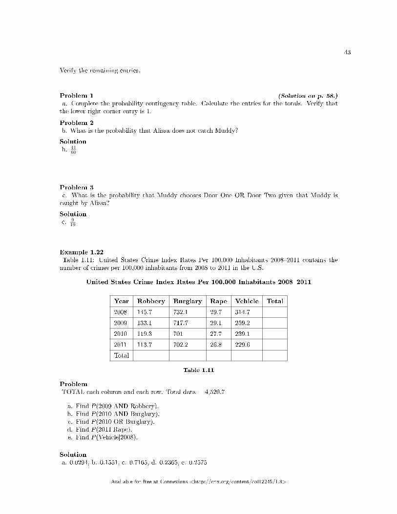
43
Verify the remaining entries.
Problem 1 (Solution on p. 58.)
a. Complete the probability contingency table. Calculate the entries for the totals. Verify thatthe lower-right corner entry is 1.
Problem 2b. What is the probability that Alissa does not catch Muddy?
Solutionb. 41
60
Problem 3c. What is the probability that Muddy chooses Door One OR Door Two given that Muddy iscaught by Alissa?
Solutionc. 9
19
Example 1.22Table 1.11: United States Crime Index Rates Per 100,000 Inhabitants 2008�2011 contains thenumber of crimes per 100,000 inhabitants from 2008 to 2011 in the U.S.
United States Crime Index Rates Per 100,000 Inhabitants 2008�2011
Year Robbery Burglary Rape Vehicle Total
2008 145.7 732.1 29.7 314.7
2009 133.1 717.7 29.1 259.2
2010 119.3 701 27.7 239.1
2011 113.7 702.2 26.8 229.6
Total
Table 1.11
ProblemTOTAL each column and each row. Total data = 4,520.7
a. Find P(2009 AND Robbery).b. Find P(2010 AND Burglary).c. Find P(2010 OR Burglary).d. Find P(2011|Rape).e. Find P(Vehicle|2008).
Solutiona. 0.0294, b. 0.1551, c. 0.7165, d. 0.2365, e. 0.2575
Available for free at Connexions <http://cnx.org/content/col12245/1.3>

44 CHAPTER 1. CHAPTER 3 - PROBABILITY TOPICS
:
Exercise 1.5.3 (Solution on p. 58.)
Table 1.12 relates the weights and heights of a group of individuals participating in anobservational study.
Weight/Height Tall Medium Short Totals
Obese 18 28 14
Normal 20 51 28
Underweight 12 25 9
Totals
Table 1.12
a.Find the total for each row and columnb.Find the probability that a randomly chosen individual from this group is Tall.c.Find the probability that a randomly chosen individual from this group is Obese andTall.
d.Find the probability that a randomly chosen individual from this group is Tall giventhat the idividual is Obese.
e.Find the probability that a randomly chosen individual from this group is Obesegiven that the individual is Tall.
f.Find the probability a randomly chosen individual from this group is Tall and Un-derweight.
g.Are the events Obese and Tall independent?
1.5.2 Tree Diagrams
Sometimes, when the probability problems are complex, it can be helpful to graph the situation. Treediagrams can be used to visualize and solve conditional probabilities.
1.5.2.1 Tree Diagrams
A tree diagram is a special type of graph used to determine the outcomes of an experiment. It consists of"branches" that are labeled with either frequencies or probabilities. Tree diagrams can make some probabilityproblems easier to visualize and solve. The following example illustrates how to use a tree diagram.
Example 1.23In an urn, there are 11 balls. Three balls are red (R) and eight balls are blue (B). Draw two balls,one at a time, with replacement. "With replacement" means that you put the �rst ball backin the urn before you select the second ball. The tree diagram using frequencies that show all thepossible outcomes follows.
Available for free at Connexions <http://cnx.org/content/col12245/1.3>

45
Figure 1.6: Total = 64 + 24 + 24 + 9 = 121
The �rst set of branches represents the �rst draw. The second set of branches represents thesecond draw. Each of the outcomes is distinct. In fact, we can list each red ball as R1, R2, and R3and each blue ball as B1, B2, B3, B4, B5, B6, B7, and B8. Then the nine RR outcomes can bewritten as:
R1R1; R1R2; R1R3; R2R1; R2R2; R2R3; R3R1; R3R2; R3R3The other outcomes are similar.There are a total of 11 balls in the urn. Draw two balls, one at a time, with replacement. There
are 11(11) = 121 outcomes, the size of the sample space.
Problem 1 (Solution on p. 59.)
a. List the 24 BR outcomes: B1R1, B1R2, B1R3, ...
Problem 2b. Using the tree diagram, calculate P(RR).
Solutionb. P(RR) =
(311
) (311
)= 9
121
Problem 3c. Using the tree diagram, calculate P(RB OR BR).
Solutionc. P(RB OR BR) =
(311
) (811
)+(
811
) (311
)= 48
121
Problem 4d. Using the tree diagram, calculate P(R on 1st draw AND B on 2nd draw).
Available for free at Connexions <http://cnx.org/content/col12245/1.3>
46 CHAPTER 1. CHAPTER 3 - PROBABILITY TOPICS
Solutiond. P(R on 1st draw AND B on 2nd draw) = P(RB) =
(311
) (811
)= 24
121
Problem 5e. Using the tree diagram, calculate P(R on 2nd draw GIVEN B on 1st draw).
Solutione. P(R on 2nd draw GIVEN B on 1st draw) = P(R on 2nd|B on 1st) = 24
88 = 311
This problem is a conditional one. The sample space has been reduced to those outcomes thatalready have a blue on the �rst draw. There are 24 + 64 = 88 possible outcomes (24 BR and 64BB). Twenty-four of the 88 possible outcomes are BR. 24
88 = 311 .
Problem 6f. Using the tree diagram, calculate P(BB).
Solutionf. P(BB) = 64
121
Problem 7 (Solution on p. 59.)
g. Using the tree diagram, calculate P(B on the 2nd draw given R on the �rst draw).
:
Exercise 1.5.4 (Solution on p. 59.)
In a standard deck, there are 52 cards. 12 cards are face cards (event F) and 40 cards arenot face cards (event N). Draw two cards, one at a time, with replacement. All possibleoutcomes are shown in the tree diagram as frequencies. Using the tree diagram, calculateP(FF).
Available for free at Connexions <http://cnx.org/content/col12245/1.3>
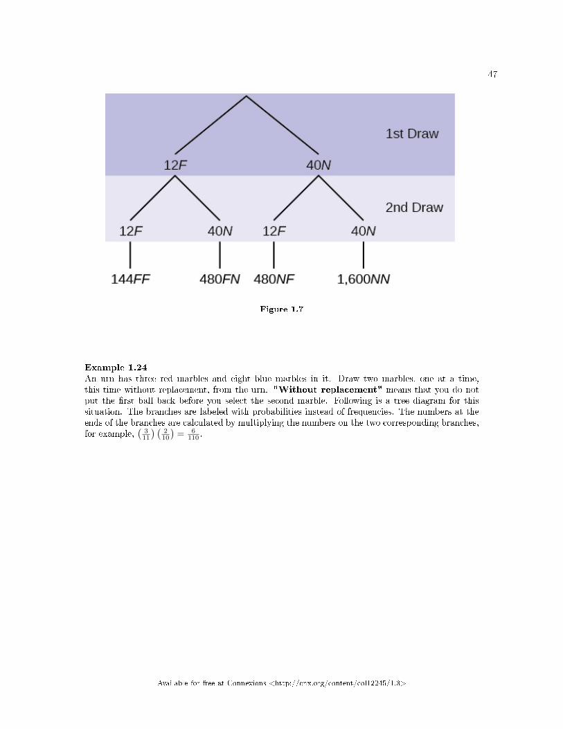
47
Figure 1.7
Example 1.24An urn has three red marbles and eight blue marbles in it. Draw two marbles, one at a time,this time without replacement, from the urn. "Without replacement" means that you do notput the �rst ball back before you select the second marble. Following is a tree diagram for thissituation. The branches are labeled with probabilities instead of frequencies. The numbers at theends of the branches are calculated by multiplying the numbers on the two corresponding branches,for example,
(311
) (210
)= 6
110 .
Available for free at Connexions <http://cnx.org/content/col12245/1.3>
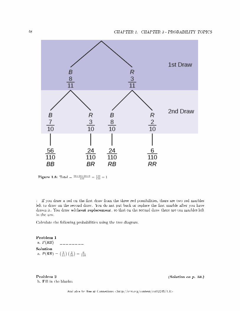
48 CHAPTER 1. CHAPTER 3 - PROBABILITY TOPICS
Figure 1.8: Total = 56+24+24+6110
= 110110
= 1
: If you draw a red on the �rst draw from the three red possibilities, there are two red marblesleft to draw on the second draw. You do not put back or replace the �rst marble after you havedrawn it. You draw without replacement, so that on the second draw there are ten marbles leftin the urn.
Calculate the following probabilities using the tree diagram.
Problem 1a. P(RR) = ________
Solutiona. P(RR) =
(311
) (210
)= 6
110
Problem 2 (Solution on p. 59.)
b. Fill in the blanks:
Available for free at Connexions <http://cnx.org/content/col12245/1.3>
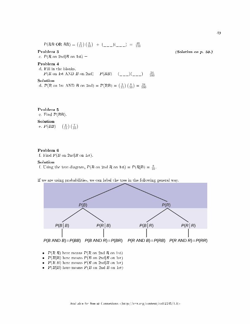
49
P(RB OR BR) =(
311
) (810
)+ (___)(___) = 48
110
Problem 3 (Solution on p. 59.)
c. P(R on 2nd|B on 1st) =
Problem 4d. Fill in the blanks.
P(R on 1st AND B on 2nd) = P(RB) = (___)(___) = 24100
Solutiond. P(R on 1st AND B on 2nd) = P(RB) =
(311
) (810
)= 24
100
Problem 5e. Find P(BB).
Solutione. P(BB) =
(811
) (710
)
Problem 6f. Find P(B on 2nd|R on 1st).
Solutionf. Using the tree diagram, P(B on 2nd|R on 1st) = P(R|B) = 8
10 .
If we are using probabilities, we can label the tree in the following general way.
• P(R|R) here means P(R on 2nd|R on 1st)• P(B|R) here means P(B on 2nd|R on 1st)• P(R|B) here means P(R on 2nd|B on 1st)• P(B|B) here means P(B on 2nd|B on 1st)
Available for free at Connexions <http://cnx.org/content/col12245/1.3>
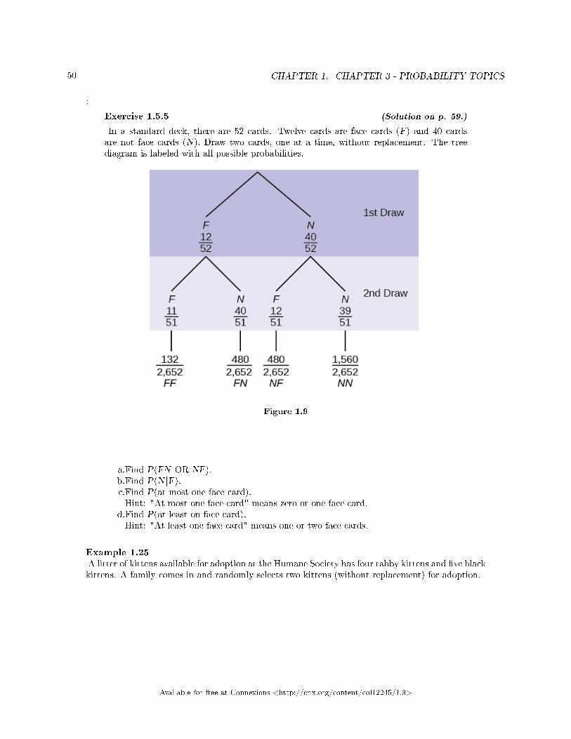
50 CHAPTER 1. CHAPTER 3 - PROBABILITY TOPICS
:
Exercise 1.5.5 (Solution on p. 59.)
In a standard deck, there are 52 cards. Twelve cards are face cards (F) and 40 cardsare not face cards (N). Draw two cards, one at a time, without replacement. The treediagram is labeled with all possible probabilities.
Figure 1.9
a.Find P(FN OR NF).b.Find P(N |F).c.Find P(at most one face card).Hint: "At most one face card" means zero or one face card.
d.Find P(at least on face card).Hint: "At least one face card" means one or two face cards.
Example 1.25A litter of kittens available for adoption at the Humane Society has four tabby kittens and �ve blackkittens. A family comes in and randomly selects two kittens (without replacement) for adoption.
Available for free at Connexions <http://cnx.org/content/col12245/1.3>
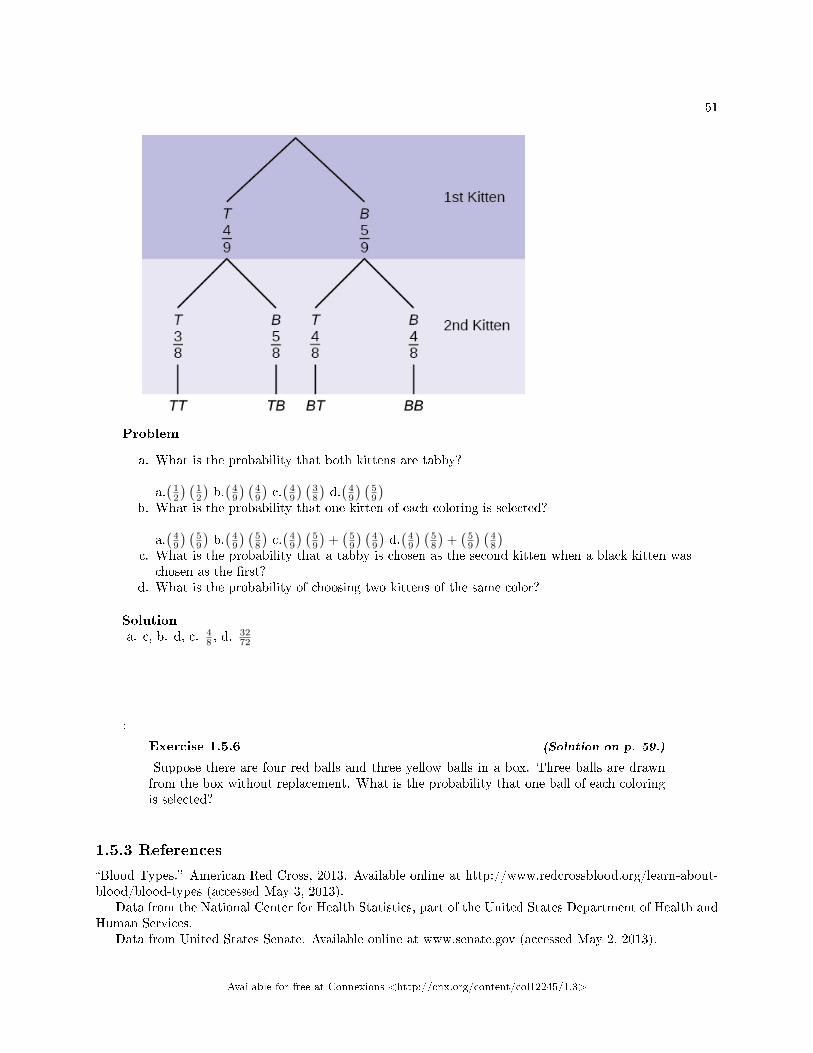
51
Problem
a. What is the probability that both kittens are tabby?
a.(12
) (12
)b.(49
) (49
)c.(49
) (38
)d.(49
) (59
)b. What is the probability that one kitten of each coloring is selected?
a.(49
) (59
)b.(49
) (58
)c.(49
) (59
)+(59
) (49
)d.(49
) (58
)+(59
) (48
)c. What is the probability that a tabby is chosen as the second kitten when a black kitten was
chosen as the �rst?d. What is the probability of choosing two kittens of the same color?
Solutiona. c, b. d, c. 4
8 , d.3272
:
Exercise 1.5.6 (Solution on p. 59.)
Suppose there are four red balls and three yellow balls in a box. Three balls are drawnfrom the box without replacement. What is the probability that one ball of each coloringis selected?
1.5.3 References
�Blood Types.� American Red Cross, 2013. Available online at http://www.redcrossblood.org/learn-about-blood/blood-types (accessed May 3, 2013).
Data from the National Center for Health Statistics, part of the United States Department of Health andHuman Services.
Data from United States Senate. Available online at www.senate.gov (accessed May 2, 2013).
Available for free at Connexions <http://cnx.org/content/col12245/1.3>
52 CHAPTER 1. CHAPTER 3 - PROBABILITY TOPICS
�Human Blood Types.� Unite Blood Services, 2011. Available online athttp://www.unitedbloodservices.org/learnMore.aspx (accessed May 2, 2013).
Haiman, Christopher A., Daniel O. Stram, Lynn R. Wilkens, Malcom C. Pike, Laurence N.Kolonel, Brien E. Henderson, and Lo�c Le Marchand. �Ethnic and Racial Di�erences in the Smoking-Related Risk of Lung Cancer.� The New England Journal of Medicine, 2013. Available online athttp://www.nejm.org/doi/full/10.1056/NEJMoa033250 (accessed May 2, 2013).
Samuel, T. M. �Strange Facts about RH Negative Blood.� eHow Health, 2013. Available online athttp://www.ehow.com/facts_5552003_strange-rh-negative-blood.html (accessed May 2, 2013).
�United States: Uniform Crime Report � State Statistics from 1960�2011.� The Disaster Center. Availableonline at http://www.disastercenter.com/crime/ (accessed May 2, 2013).
Data from Clara County Public H.D.Data from the American Cancer Society.Data from The Data and Story Library, 1996. Available online at http://lib.stat.cmu.edu/DASL/ (ac-
cessed May 2, 2013).Data from the Federal Highway Administration, part of the United States Department of Transportation.Data from the United States Census Bureau, part of the United States Department of Commerce.Data from USA Today.�Environment.� The World Bank, 2013. Available online at
http://data.worldbank.org/topic/environment (accessed May 2, 2013).�Search for Datasets.� Roper Center: Public Opinion Archives, University of Connecticut., 2013. Avail-
able online at http://www.ropercenter.uconn.edu/data_access/data/search_for_datasets.html (accessedMay 2, 2013).
1.5.4 Chapter Review
There are several tools you can use to help organize and sort data when calculating probabilities. Contin-gency tables help display data and are particularly useful when calculating probabilites that have multipledependent variables.
A tree diagram use branches to show the di�erent outcomes of experiments and makes complex probabilityquestions easy to visualize.
Available for free at Connexions <http://cnx.org/content/col12245/1.3>
53
Solutions to Exercises in Chapter 1
to Exercise 1.2.1 (p. 6)
a. S = {(1,1), (1,2), (1,3), (1,4), (2,1), (2,2), (2,3), (2,4), (3,1), (3,2), (3,3), (3,4)}b. A = {(1,1), (1,3), (2,2), (2,4), (3,1), (3,3)}
B = {(2,1), (2,2), (2,3), (2,4), (3,1), (3,2), (3,3), (3,4)}c. P(A) = 1
2 , P(B) =23
d. A AND B = {(2,2), (2,4), (3,1), (3,3)}
A OR B = {(1,1), (1,3), (2,1), (2,2), (2,3), (2,4), (3,1), (3,2), (3,3), (3,4)}e. P(A AND B) = 1
3 , P(A OR B) = 56
f. B′ = {(1,1), (1,2), (1,3), (1,4)}, P(B′) = 13
g. P(B) + P(B′) = 1
h. P(A|B) = P (AANDB)P (B) = 1
2 , P(B|A) =P (AANDB)
P (B) = 23 , No.
Solution to Exercise 1.2.2 (p. 9)
a. P(L′) = P(S)b. P(M OR S)c. P(F AND L)d. P(M |L)e. P(L|M)f. P(S|F)g. P(F|L)h. P(F OR L)i. P(M AND S)j. P(F)
Solution to Exercise 1.2.4 (p. 9)P(N) = 15
42 = 514 = 0.36
Solution to Exercise 1.2.6 (p. 9)P(C) = 5
42 = 0.12Solution to Exercise 1.2.8 (p. 10)P(G) = 20
150 = 215 = 0.13
Solution to Exercise 1.2.10 (p. 10)P(R) = 22
150 = 1175 = 0.15
Solution to Exercise 1.2.12 (p. 10)P(O) = 150−22−38−20−28−26
150 = 16150 = 8
75 = 0.11Solution to Exercise 1.2.14 (p. 10)P(E) = 47
194 = 0.24Solution to Exercise 1.2.16 (p. 10)P(N) = 23
194 = 0.12Solution to Exercise 1.2.18 (p. 10)P(S) = 12
194 = 697 = 0.06
Solution to Exercise 1.2.20 (p. 10)1352 = 1
4 = 0.25Solution to Exercise 1.2.22 (p. 10)36 = 1
2 = 0.5Solution to Exercise 1.2.24 (p. 11)P (R) = 4
8 = 0.5
Available for free at Connexions <http://cnx.org/content/col12245/1.3>
54 CHAPTER 1. CHAPTER 3 - PROBABILITY TOPICS
Solution to Exercise 1.2.26 (p. 11)P(O OR H)Solution to Exercise 1.2.28 (p. 12)P(H |I)Solution to Exercise 1.2.30 (p. 12)P(N |O)Solution to Exercise 1.2.32 (p. 12)P(I OR N)Solution to Exercise 1.2.34 (p. 12)P(I)Solution to Exercise 1.2.36 (p. 12)The likelihood that an event will occur given that another event has already occurred.Solution to Exercise 1.2.38 (p. 12)1Solution to Exercise 1.2.40 (p. 12)the probability of landing on an even number or a multiple of threeSolution to Exercise 1.2.42 (p. 13)
a. You can't calculate the joint probability knowing the probability of both events occurring, which is notin the information given; the probabilities should be multiplied, not added; and probability is nevergreater than 100%
b. A home run by de�nition is a successful hit, so he has to have at least as many successful hits as homeruns.
to Exercise 1.3.1 (p. 14)
a. With replacementb. No
Solution to Exercise 1.3.2 (p. 15)without replacement: 1. Possible; 2. Impossible, 3. Possible
with replacement: 1. Possible; 2. Possible, 3. Possibleto Exercise 1.3.3 (p. 16)
a. P(F) = 14
b. P(G) = 12
c. P(H) = 12
d. Yese. No
to Exercise 1.3.4 (p. 17)
P(A|B) = P (A AND B)P (B) = 0.08
0.2 = 0.4 = P (A)
The events are independent because P(A|B) = P(A).to Exercise 1.3.5 (p. 18)Event G and O = {G1, G3}
P(G and O) = 210 = 0.2
to Exercise 1.3.6 (p. 18)
a. P(B|D) = 0.6667b. P(D|B) = 0.5c. Nod. No
Available for free at Connexions <http://cnx.org/content/col12245/1.3>
55
to Exercise 1.3.7 (p. 19)P(B|A) = 0.67
P(B) = 0.25So P(B) does not equal P(B|A) which means that B and A are not independent (wearing blue and
rooting for the away team are not independent). They are also not mutually exclusive, because P(B ANDA) = 0.20, not 0.to Exercise 1.3.8 (p. 20)Because P(I AND F) = 0,
P(I OR F) = P(I) + P(F) - P(I AND F) = 0.44 + 0.56 - 0 = 1Solution to Exercise 1.3.9 (p. 21)
a. P(T) = 14
b. P(T|F) = 12
c. Nod. Noe. Yes
to Exercise 1.3.11 (p. 22)P(J) = 0.3to Exercise 1.3.13 (p. 22)P(Q AND R) = P(Q)P(R)
0.1 = (0.4)P(R)P(R) = 0.25
Solution to Exercise 1.3.15 (p. 23)0Solution to Exercise 1.3.17 (p. 23)0.3571to Exercise 1.3.19 (p. 23)0.2142to Exercise 1.3.21 (p. 23)Physician (83.7)to Exercise 1.3.23 (p. 24)83.7 − 79.6 = 4.1to Exercise 1.3.25 (p. 24)P(Occupation < 81.3) = 0.5to Exercise 1.3.27 (p. 24)
a. P(C) = 0.4567b. not enough informationc. not enough informationd. No, because over half (0.51) of men have at least one false positive text
to Exercise 1.3.29 (p. 24)
a. P(J OR K) = P(J) + P(K) − P(J AND K); 0.45 = 0.18 + 0.37 - P(J AND K); solve to �nd P(JAND K) = 0.10
b. P(NOT (J AND K)) = 1 - P(J AND K) = 1 - 0.10 = 0.90c. P(NOT (J OR K)) = 1 - P(J OR K) = 1 - 0.45 = 0.55
to Exercise 1.4.1 (p. 26)P(D|C) = 0.85
P(C ∩ D) = P(D ∩ C)P(D ∩ C) = P(D|C)P(C) = (0.85)(0.75) = 0.6375Helen makes the �rst and second free throws with probability 0.6375.
Available for free at Connexions <http://cnx.org/content/col12245/1.3>
56 CHAPTER 1. CHAPTER 3 - PROBABILITY TOPICS
to Exercise 1.4.2 (p. 28)P = 200−140−40
200 = 20200 = 0.1
to Exercise 1.4.3 (p. 28)
a. P(B ∩ D) = P(D|B)P(B) = (0.5)(0.4) = 0.20.b. P(B ∪ D) = P(B) + P(D) − P(B ∩ D) = 0.40 + 0.30 − 0.20 = 0.50
to Exercise 1.4.4 (p. 30)Let A = student is a senior going to college.
Let B = student plays sports.P(B) = 140
200P(B|A) = 50
140P(A ∩ B) = P(B|A)P(A)P(A ∩ B) =
(140200
) (50140
)= 1
4to Exercise 1.4.5 (p. 30)
a. P(B′) = 0.60b. P(D ∩ B) = P(D|B)P(B) = 0.20
c. P(B|D) = P (B∩D)P (D) = (0.20)
(0.30) = 0.66
d. P(D ∩ B′) = P(D) - P(D ∩ B) = 0.30 - 0.20 = 0.10e. P(D|B′) = P(D ∩ B′)P(B′) = (P(D) - P(D ∩ B))(0.60) = (0.10)(0.60) = 0.06
Solution to Exercise 1.4.7 (p. 32)0.376Solution to Exercise 1.4.9 (p. 32)C |L means, given the person chosen is a Latino Californian, the person is a registered voter who prefers lifein prison without parole for a person convicted of �rst degree murder.Solution to Exercise 1.4.11 (p. 32)L ∩ C is the event that the person chosen is a Latino California registered voter who prefers life withoutparole over the death penalty for a person convicted of �rst degree murder.Solution to Exercise 1.4.13 (p. 32)0.6492Solution to Exercise 1.4.15 (p. 32)No, because P(L ∩ C) does not equal 0.Solution to Exercise 1.4.17 (p. 33)
a. The Forum Research surveyed 1,046 Torontonians.b. 58%c. 42% of 1,046 = 439 (rounding to the nearest integer)d. 0.57e. 0.60.
Solution to Exercise 1.4.19 (p. 34)
a. P(Betting on two line that touch each other on the table) = 638
b. P(Betting on three numbers in a line) = 338
c. P(Bettting on one number) = 138
d. P(Betting on four number that touch each other to form a square) = 438
e. P(Betting on two number that touch each other on the table ) = 238
f. P(Betting on 0-00-1-2-3) = 538
g. P(Betting on 0-1-2; or 0-00-2; or 00-2-3) = 338
Solution to Exercise 1.4.21 (p. 35)
a. {G1, G2, G3, G4, G5, Y1, Y2, Y3}
Available for free at Connexions <http://cnx.org/content/col12245/1.3>
57
b. 58
c. 23
d. 28
e. 68
f. No, because P(G ∩ E) does not equal 0.
Solution to Exercise 1.4.23 (p. 35)
: The coin toss is independent of the card picked �rst.
a. {(G,H) (G,T) (B,H) (B,T) (R,H) (R,T)}b. P(A) = P(blue)P(head) =
(310
)(12
)= 3
20c. Yes, A and B are mutually exclusive because they cannot happen at the same time; you cannot pick
a card that is both blue and also (red or green). P(A ∩ B) = 0d. No, A and C are not mutually exclusive because they can occur at the same time. In fact, C includes
all of the outcomes of A; if the card chosen is blue it is also (red or blue). P(A ∩ C) = P(A) = 320
Solution to Exercise 1.4.25 (p. 36)
a. S = {(HHH), (HHT), (HTH), (HTT), (THH), (THT), (TTH), (TTT)}b. 4
8c. Yes, because if A has occurred, it is impossible to obtain two tails. In other words, P(A ∩ B) = 0.
Solution to Exercise 1.4.27 (p. 36)
a. If Y and Z are independent, then P(Y ∩ Z) = P(Y )P(Z), so P(Y ∪ Z) = P(Y ) + P(Z) - P(Y )P(Z).b. 0.5
Solution to Exercise 1.4.29 (p. 36)a. iii; a. i; a. iv; a. iiSolution to Exercise 1.4.31 (p. 37)
a. P(R) = 0.44b. P(R|E) = 0.56c. P(R|O) = 0.31d. No, whether the money is returned is not independent of which class the money was placed in. There
are several ways to justify this mathematically, but one is that the money placed in economics classesis not returned at the same overall rate; P(R|E) 6= P(R).
e. No, this study de�nitely does not support that notion; in fact, it suggests the opposite. The moneyplaced in the economics classrooms was returned at a higher rate than the money place in all classescollectively; P(R|E) > P(R).
Solution to Exercise 1.4.33 (p. 38)
a. P(type O ∪ Rh-) = P(type O) + P(Rh-) - P(type O ∩ Rh-)0.52 = 0.43 + 0.15 - P(type O ∩ Rh-); solve to �nd P(type O ∩ Rh-) = 0.066% of people have type O, Rh- blood
b. P(NOT(type O ∩ Rh-)) = 1 - P(type O ∩ Rh-) = 1 - 0.06 = 0.9494% of people do not have type O, Rh- blood
Solution to Exercise 1.4.35 (p. 38)
a. Let C = be the event that the cookie contains chocolate. Let N = the event that the cookie containsnuts.
b. P(C ∪ N) = P(C) + P(N) - P(C ∩ N) = 0.36 + 0.12 - 0.08 = 0.40
Available for free at Connexions <http://cnx.org/content/col12245/1.3>
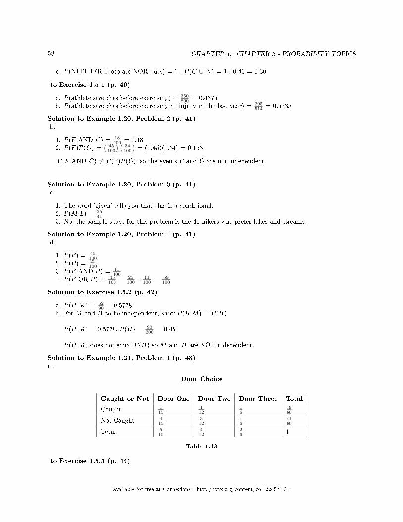
58 CHAPTER 1. CHAPTER 3 - PROBABILITY TOPICS
c. P(NEITHER chocolate NOR nuts) = 1 - P(C ∪ N) = 1 - 0.40 = 0.60
to Exercise 1.5.1 (p. 40)
a. P(athlete stretches before exercising) = 350800 = 0.4375
b. P(athlete stretches before exercising|no injury in the last year) = 295514 = 0.5739
Solution to Example 1.20, Problem 2 (p. 41)b.
1. P(F AND C) = 18100 = 0.18
2. P(F)P(C) =(
45100
) (34100
)= (0.45)(0.34) = 0.153
P(F AND C) 6= P(F)P(C), so the events F and C are not independent.
Solution to Example 1.20, Problem 3 (p. 41)c.
1. The word 'given' tells you that this is a conditional.2. P(M |L) = 25
413. No, the sample space for this problem is the 41 hikers who prefer lakes and streams.
Solution to Example 1.20, Problem 4 (p. 41)d.
1. P(F) = 45100
2. P(P) = 25100
3. P(F AND P) = 11100
4. P(F OR P) = 45100 + 25
100 - 11100 = 59
100
Solution to Exercise 1.5.2 (p. 42)
a. P(H |M) = 5290 = 0.5778
b. For M and H to be independent, show P(H |M) = P(H)
P(H |M) = 0.5778, P(H) = 90200 = 0.45
P(H |M) does not equal P(H) so M and H are NOT independent.
Solution to Example 1.21, Problem 1 (p. 43)a.
Door Choice
Caught or Not Door One Door Two Door Three Total
Caught 115
112
16
1960
Not Caught 415
312
16
4160
Total 515
412
26 1
Table 1.13
to Exercise 1.5.3 (p. 44)
Available for free at Connexions <http://cnx.org/content/col12245/1.3>

59
Weight/Height Tall Medium Short Totals
Obese 18 28 14 60
Normal 20 51 28 99
Underweight 12 25 9 46
Totals 50 104 51 205
Table 1.14
a. Row Totals: 60, 99, 46. Column totals: 50, 104, 51.b. P(Tall) = 50
205 = 0.244c. P(Obese AND Tall) = 18
205 = 0.088d. P(Tall|Obese) = 18
60 = 0.3e. P(Obese|Tall) = 18
50 = 0.36f. P(Tall AND Underweight = 12
205 = 0.0585g. No. P(Tall) does not equal P(Tall|Obese).
Solution to Example 1.23, Problem 1 (p. 45)a. B1R1; B1R2; B1R3; B2R1; B2R2; B2R3; B3R1; B3R2; B3R3; B4R1; B4R2; B4R3; B5R1; B5R2;B5R3; B6R1; B6R2; B6R3; B7R1; B7R2; B7R3; B8R1; B8R2; B8R3
Solution to Example 1.23, Problem 7 (p. 46)g. P(B on 2nd draw|R on 1st draw) = 8
11There are 9 + 24 outcomes that have R on the �rst draw (9 RR and 24 RB). The sample space is then
9 + 24 = 33. 24 of the 33 outcomes have B on the second draw. The probability is then 2433 .
to Exercise 1.5.4 (p. 46)Total number of outcomes is 144 + 480 + 480 + 1600 = 2,704.
P(FF) = 144144 + 480 + 480 + 1,600 = 144
2,704 = 9169
Solution to Example 1.24, Problem 2 (p. 48)b. P(RB OR BR) =
(311
) (810
)+(
811
) (310
)= 48
110
Solution to Example 1.24, Problem 3 (p. 49)c. P(R on 2nd|B on 1st) = 3
10
to Exercise 1.5.5 (p. 50)
a. P(FN OR NF) = 4802,652 + 480
2,652 = 9602,652 = 80
221
b. P(N |F) = 4051
c. P(at most one face card) = (480 + 480 + 1,560)2,652 = 2,520
2,652
d. P(at least one face card) = (132 + 480 + 480)2,652 = 1,092
2,652
to Exercise 1.5.6 (p. 51)(47
) (36
)+(37
) (46
)
Available for free at Connexions <http://cnx.org/content/col12245/1.3>

60 CHAPTER 1. CHAPTER 3 - PROBABILITY TOPICS
Available for free at Connexions <http://cnx.org/content/col12245/1.3>
Chapter 2
Chapter 4 - Binomial Distribution
2.1 Introduction to Discrete Probability Distributions - MRU - CLemieux (2017)1
2.1.1 Introduction
2.1.1.1 Chapter Objectives
By the end of this chapter, the student should be able to:
• Recognize the binomial probability distribution and apply it appropriately.• Be able to evaluate evidence using the binomial distribution.
Suppose you �ip a coin ten times and each time it comes up heads. This might make you start to wonder ifthere is something wrong with the coin. Perhaps it is a trick coin and is heads on both sides? Perhaps it isimbalanced and it is more likely to come up heads over tails. You may also wonder what is the probabilityof getting 10 heads in a row, if the coin was fair.
Coin �ipping is interesting because it is a random event. We cannot predict whether the next �ip willbe heads or tails (assuming it isn't a trick coin). That means the outcome would be a random variable. Arandom variable is any variable where the outcome is determined by a random event. The outcome isalso discrete because we count it. Above you �ipped a coin ten times and counted the number of heads. Adiscrete random variable is a variable whose outcome is determined by a random event and where wecount the outcomes. Other examples of discrete random variables include how many times you roll an evennumber with a die out of ten rolls; how many customers enter a store during a �ve-minute interval; howmany times you draw a high card out of a deck of cards out of eight draws (without replacement).
In each of these situations (coin toss, rolling die, number of customers, drawing cards), you could look ateach situation and, each time, come up with a new formula to �nd the probability of these events happening.But this would take a lot of work and be ine�cient. Instead, you would want to see if the situation can bemodelled by a distribution. A probability distribution provides the theoretical probabilities of all of thepossible events in a situation. For example, the following is a probability model of how many heads you canget when you �ip a fair coin three times:
1This content is available online at <http://cnx.org/content/m64919/1.1/>.
Available for free at Connexions <http://cnx.org/content/col12245/1.3>
61
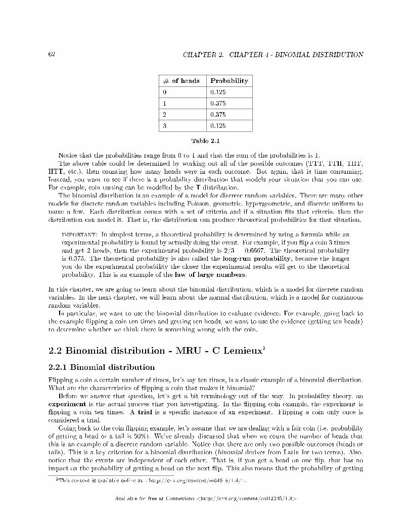
62 CHAPTER 2. CHAPTER 4 - BINOMIAL DISTRIBUTION
# of heads Probability
0 0.125
1 0.375
2 0.375
3 0.125
Table 2.1
Notice that the probabilities range from 0 to 1 and that the sum of the probabilities is 1.The above table could be determined by working out all of the possible outcomes (TTT, TTH, THT,
HTT, etc.), then counting how many heads were in each outcome. But again, that is time consuming.Instead, you want to see if there is a probability distribution that models your situation that you can use.For example, coin tossing can be modelled by the T distribution.
The binomial distribution is an example of a model for discrete random variables. There are many othermodels for discrete random variables including Poisson, geometric, hypergeometric, and discrete uniform toname a few. Each distribution comes with a set of criteria and if a situation �ts that criteria, then thedistribution can model it. That is, the distribution can produce theoretical probabilities for that situation.
important: In simplest terms, a theoretical probability is determined by using a formula while anexperimental probability is found by actually doing the event. For example, if you �ip a coin 3 timesand get 2 heads, then the experimental probability is 2/3 = 0.6667. The theoretical probabilityis 0.375. The theoretical probability is also called the long-run probability, because the longeryou do the experimental probability the closer the experimental results will get to the theoreticalprobability. This is an example of the law of large numbers.
In this chapter, we are going to learn about the binomial distribution, which is a model for discrete randomvariables. In the next chapter, we will learn about the normal distribution, which is a model for continuousrandom variables.
In particular, we want to use the binomial distribution to evaluate evidence. For example, going back tothe example �ipping a coin ten times and getting ten heads, we want to use the evidence (getting ten heads)to determine whether we think there is something wrong with the coin.
2.2 Binomial distribution - MRU - C Lemieux2
2.2.1 Binomial distribution
Flipping a coin a certain number of times, let's say ten times, is a classic example of a binomial distribution.What are the characteristics of �ipping a coin that makes it binomial?
Before we answer that question, let's get a bit terminology out of the way. In probability theory, anexperiment is the actual process that you investigating. In the �ipping coin example, the experiment is�ipping a coin ten times. A trial is a speci�c instance of an experiment. Flipping a coin only once isconsidered a trial.
Going back to the coin �ipping example, let's assume that we are dealing with a fair coin (i.e. probabilityof getting a head or a tail is 50%). We've already discussed that when we count the number of heads thatthis is an example of a discrete random variable. Notice that there are only two possible outcomes (heads ortails). This is a key criterion for a binomial distribution (binomial derives from Latin for two terms). Also,notice that the events are independent of each other. That is, if you get a head on one �ip, that has noimpact on the probability of getting a head on the next �ip. This also means that the probability of getting
2This content is available online at <http://cnx.org/content/m64918/1.4/>.
Available for free at Connexions <http://cnx.org/content/col12245/1.3>
63
a head remains constant. This is another key criterion for a binomial distribution. The other thing to noticeis that the number of times we �ip the coin is �xed. We don't �ip it until we get bored or run out of time.Instead we �ip it ten times. This means that the number of trials is �xed. This is the last key criterion of abinomial distribution.
There are �ve characteristics of a binomial experiment.
1. The variable being studied is random.2. The outcomes of the variable are being counted.3. There are a �xed number of trials. The letter n denotes the number of trials.4. There are only two possible outcomes, called "success" and "failure," for each trialπ denotes the
probability of a success on one trial, and 1-π denotes the probability of a failure on one trial.5. The n trials are independent and are repeated using identical conditions. Because the n trials are
independent, the outcome of one trial does not help in predicting the outcome of another trial. Anotherway of saying this is that for each individual trial, the probability, π, of a success and probability, 1-π,of a failure remain constant.
Other examples of binomial distributions:
• Counting the number of 2's that are rolled when you roll a die six times (trial = rolling a dice, success= rolling a 2, n = 6, π = 1/6 = 0.1667)
• Counting the number of times a jack is pulled out of deck of cards (with replacement) when you pulla card �fteen times (trial = pulling a card, success = pulling a jack, n = 15, π = 4/52 = 0.0769)
• Counting the number of times that you win a prize in Tim Hortons Roll up the Rim to Win contestout of four cups (trial = checking cup for win, success = winning a prize, n = 4, π = 1/6 = 0.1667 �assuming no special rules (e.g. anniversary rules that changed the odds of winning)
Examples of situations that are not binomial include:
• Counting the number of times a jack is pulled out of deck of cards (without replacement) when youpull a card �fteen times. The �fth criterion is not met because the events are now dependent.
• Counting the number times each number (1 to 6) is rolled when you roll a die �fty times. The fourthcriterion is not met because there are six possible outcomes instead of two.
• Counting the number of times that you win a prize in Tim Horton's Roll up the Rim to Win contestout of how many cups you buy during the contest. Unless you know exactly how many you'll buyduring the contest, this would not meet the third criterion of having a �xed number of trials.
note: The Roll up the Rim example might not be binomial as it may fail the �fth criterion. At thebeginning of the contest, the odds of winning are determined by counting how many prizes thereare out of the total number of cups printed. As the contest goes on, the probability of winning maychange depending on how many people have already won. At the beginning of the contest, thisis also true but there are so many cups that it doesn't really matter (think back to the samplingwith replacement vs. without replacement in Chapter 1). Thus, this contest is only binomial atthe beginning of the contest.
2.2.2 Notation
Suppose we are working on a probability question and there are multiple probabilities that need to be found.Then it gets time consuming to write out, for example, �the probability that three rolls of a die will resultin at least one 2� or some variation over and over again. Instead we will use notation to reduce the work.We can write the previous statement more quickly as P(X ≥ 1). The P( ) means the �probability of�. X isthe random variable being studied (in this case the number of times 2 has been rolled out of 3 rolls). �X ≥1� means we are looking at the number of times a 2 is rolled at least once.
It is important to de�ne X. Otherwise, P(2<X≤ 5) could refer to any random variable and the personreading the notation won't know what it means.
Available for free at Connexions <http://cnx.org/content/col12245/1.3>

64 CHAPTER 2. CHAPTER 4 - BINOMIAL DISTRIBUTION
2.2.2.1 Mean and standard deviation of the binomial distribution
Just like a set of data, a binomial distribution has a mean and a standard deviation. For the binomialdistribution, these are given by the formulas:
µ = nπσ =
√nπ (1− π)
Going back to the Tim Hortons example, we had n=4 and π= 0.1667. Thus µ = 4 × 0.1667= 0.6667and σ =
√4× 0.1667× (1− 0.1667) = 0.745. This means that if we buy four random cups of Tim Hortons
co�ee during the Roll Up the Rim content, we will typically win 0.67 times, give or take 0.75. Thus, whenbuying four cups of co�ee, we will typically win between -0.08 and 1.42 times. Since we can't win negativetimes, we will round the lower bound to 0. Therefore, when buying four cups of co�ee, we will typically winbetween 0 and 1.42 times.
Exercise 2.2.1 (Solution on p. 74.)
A market research study shows that 30% of all passengers on Canadian Airlines are businesstravelers. A random sample of 20 passengers is taken.
1. Explain why the above situation satis�es the criteria of a binomial distribution. If there areany issues with why this situation may not meet all of the criteria, discuss them. De�ne n, Xand π.
2. For the random sample, determine the probability that:
a. Exactly seven of the passengers are business travelers.b. From ten to fourteen (inclusive) are business travelers.c. At least eleven of these passengers are business travelers.d. Five of these passengers are NOT travelling on business.
3. What is the typical range of business passengers in a random sample of 20?
2.2.3 Evaluating evidence using the binomial distribution
A company looked at its hiring practices. In particular, they found that their hiring practices appears tofavour men over women. Based on past data, they have found that regardless of the number of applicationsby women, seventy-�ve percent of hires are men. Due to this issue, they decide to implement program.In this program, the name and any identifying features that may indicate the gender of an applicant areremoved. For example, if the application says, �She executed a marketing campaign that increased revenueby 30%�, this would be changed to �They executed a marketing campaign that increased revenue by 30%.�The names on the applications were changed an alpha-numeric identi�cation (like AB-101). The companyclaims that the program has worked, but they want to check the claim.
How will the company determine if the program has worked? One way to do this would be using statistics.Now suppose that after a recent round of hiring, the proportion of men hired was 70%. Would this be
enough evidence that the program is working? 70% is de�nitely lower than 75%, but we know that there isvariability in sampling. This means that, prior to the program being implemented, around 75% of hires aremen, there may be some rounds of hiring where 70% of hires were men and some that were 80%. It won'tbe 75% each time. Instead we expect it to be close to 75%. Therefore, if the program has caused the hiringpractices to change, would a recent round of hiring that results in the proportion of men hires being 70%be enough evidence of change? What about 60%? What is the line between normal variability from 75%and abnormal variability? Statistics helps us �gure that out and that is how we evaluate evidence usingstatistics.
Let's say in a recent round of hires there were 30 new hires and 20 of these hires were men.
Available for free at Connexions <http://cnx.org/content/col12245/1.3>
65
2.2.3.1 Skepticism
Any time we are trying to evaluate evidence, we always start from a position of skepticism. That is, we don'twant to assume what we are trying to show (i.e the claim). If we do that, we may bias the investigation. Toillustrate, if you assume that your signi�cant other is cheating on you, then this will colour all of the evidenceyou �nd (why did they show up �ve minutes late from work? They must be cheating!). A well-known real-world example of this position is the assumption in court that a defendant is innocent until proven guilty.That is, criminal court cases start with the assumption of innocence.
In general, the position of skepticism is that nothing has changed, the program didn't work, the experi-ment didn't work, the e�ect being studied isn't happening, etc.
In our example, we will assume that the program that the company implemented did not work. That is,we are assuming that the proportion of hires that are men is still 75%. Another way of writing this is π =75% (i.e. the population proportion).
2.2.3.2 Evidence
In a court case, evidence would be witness testimony, forensics evidence, expert testimony, etc.In statistics, evidence is sample data. The evidence has been collected to evaluate the claim. In this case,
the evidence has been evaluated to determine if the program is working.In our example, the sample data is the 20 men hires out of 30. This gives us a sample proportion of
20/30 = 66.67%. The symbol for sample proportion is^p (said �p hat� - the symbol above the p is supposed
to be "^", but the online textbook program does not properly show it).
2.2.3.3 Evaluating evidence in statistics
To evaluate the evidence, we want to determine the probability of observing the evidence (or even betterevidence against the assumption) assuming the assumption is true. Once we determine this probability, weneed to determine if the event is unlikely or not unlikely. That is, we want to determine if it unlikely we couldhave observed the evidence, if the assumption is true. Or is it not unlikely that we observed the evidence, ifthe assumption is true. If it is unlikely to have observed the evidence, then most likely there is somethingwrong with the assumption and the claim is likely true. If it is not unlikely to have observed the evidence,then we can't actually conclude that there is something wrong with the assumption and we cannot concludethat the claim is true.
To go back to the court case example, if you are a juror, you have to evaluate how unlikely or not unlikelyit is that the defendant would have had a heated argument with the victim, and was found covered in bloodand holding the murder weapon at the scene, if the defendant was innocent. If you think that it is unlikelythat all of the pieces of evidence could have happened if the defendant is innocent, then you would �nd thedefendant guilty. That is, the evidence calls into question the assumption. If you think that this it is notunlikely that all of these pieces of evidence could have happened if the defendant is innocent, then you would�nd the defendant not guilty. Notice that we don't conclude that the defendant is innocent. That is, wecan't say that they are innocent; we can only say that they are not guilty.
note: When evaluating evidence, we are trying to evaluate the claim (i.e. not the position ofskepticism). Therefore, the evidence has been collected about claim. No evidence has been col-lected about the assumption. Therefore, our conclusion can only be about the claim and not theassumption.
Therefore, if the probability is small and therefore unlikely, we can say that there is enough evidence tosuggest that the assumption is likely false (i.e. guilty).
If the probability is not small and therefore not unlikely, we can say that there is not enough evidence tosuggest that the assumption is false (i.e. not guilty).
Available for free at Connexions <http://cnx.org/content/col12245/1.3>
66 CHAPTER 2. CHAPTER 4 - BINOMIAL DISTRIBUTION
note: In statistics, if the probability of an event happening is less than 1%, we say that the eventis unlikely to happen. If the probability is greater than 10%, we say the event is not unlikely tohappen. If the probability is between 1% and 10%, then it is up to the researcher to determinewhether they believe that the event is unlikely or not unlikely. Usually, the researcher decides onthe threshold between unlikely and not unlikely before performing the experiment or study.
In our example, to evaluate the evidence, we want to work out what is the probability this company wouldhave hired 20 men out 30 (or even better evidence against the assumption) if the proportion of men hires isstill 75%. That is, we want to �nd P (X ≤ 20) , given π = 75%). Notice that this is a conditional probabilityand the condition is the assumption.
What does �or even better evidence against the assumption� mean? It means that we don't just �nd theprobability of exactly 20 out of 30 men hires. We �nd the probability of at most 20 out of 30 men hiresbecause if the company hired 19, 18, 17, . . . men then that would be even better evidence that 75% is nolonger correct (as the sample proportion is getting more and more di�erent from the assumed populationproportion).
Why do we look at �or even better evidence against the assumption�? Often the probability of exactlyone event happening is quite small. For example, the probability of getting exactly 10 heads out of 20 cointosses is 17.62%, even though that is the most likely event to occur. Therefore, if we only looked at theprobability of exactly one event happening (i.e. P(X=20)) rather than P (X ≤ 20) , we may come to thefalse impression that an event is unlikely, when it could actually be explained by normal sampling variability.
2.2.3.4 Finding the probability
To �nd the probability, we need to �nd an appropriate distribution that models the situation. In laterchapters, we will look at other models. Right now, the model we are going to use is the binomial distribution.For us to use this model, we have to ensure that the situation is meeting all of the conditions of the binomialdistribution.
1. The variable being studied is random: This is not necessarily the case here as the applicants are notrandom and the hiring process is not random. If we randomly selected 30 hires from a greater numberof hires, then it would be.
2. The outcomes of the variable are being counted: We are counting the number of men hired.3. There are a �xed number of trials: We are looking at 30 hires (n = 30)4. There are only two possible outcomes: Either the hire is a man or the hire is not a man.5. The n trials are independent and the probability of success and probability of failure remain constant:
This is true because we are assuming that the probability of hiring a man remains constant at 75%.
Though the �rst condition is not met, we can still use the binomial distribution to model the situation. Thatthe model is not perfectly met would be a limitation of the study. That means that we would want to puta caveat at the end of our conclusion to state that this might reduce the accuracy of our results.
warning: If the conditions of randomness and independence may not be fully met, then we canstill utilize the binomial distribution. But we do have to be wary of the results. The other threeconditions do need to be met to use the binomial distribution.
Now that we have the model, we can �nd the probability. In A computer program, we will use the binomialdistribution with n = 30 and π (or probability of occurrence) = 0.75. Then we will �nd P (X ≤ 20) .
From the computer program, we get P (X ≤ 20) = 0.19659 = 19.659. Again, this probability is foundunder the assumption that the program has not worked (i.e. π=75%)
2.2.3.5 Evaluating the probability
The probability that we would have observed at most 20 hires that were men out of 30, under the assumptionthat the program did not work, is 19.659%. Therefore, it is not unlikely that we could have observed this
Available for free at Connexions <http://cnx.org/content/col12245/1.3>
67
evidence as the probability is greater than 10%. This means that having 20 out of 30 hires being men fallswithin the normal sampling variability for this data.
Based on the evidence collected, there is not su�cient evidence to suggest that the program worked.Notice we don't conclude that the program is not working.
note: In statistics, we never use the words �prove� or �true� when making a conclusion. All ofour conclusions are based o� of sample data that we are using to make a conclusion about thepopulation. Therefore, there is always the chance of error.
2.2.3.6 Example
Olivier has spent �ve years honing his archery skills in various seedy locals around the world. Now he hasreturned to his city of birth to use these skills to take out criminals. One night while drinking vodka withhis friends, he boasts that he can shoot an arrow into the bullseye, blindfolded at a distance of 50m 90% ofthe time.
�I don't believe you!� Jack, Olivier's best friend, slurred.�I swear! I've really honed my skills.� Olivier countered.�But remember last week when we were in that darkened factory, you missed two of your shots!� Thelma,
Olivier's sister, countered.�No. I meant to miss them.�Jack thought for a moment. �I think you are exaggerating and I'm going to test you.��You're on!� Olivier sneered arrogantly.To test that Olivier was exaggerating about his marksmanship, Jack set up a bunch of targets and,
randomly had Olivier attempt the shot. Olivier hit the bullseye (blindfolded at a distance of 50m) 39 out of50 times.
a. If Olivier's is not exaggerating, how many times out of 50 do we typically expect him to hit the bullseye?Write your answer as a range that takes into account variation.
Answer: We would expect Olivier to hit the bullseye 45 times give or take 2.121 times. This means a typicalrange is 42.88 to 47.12 bullseyes out of 50.
b. Based on your answer in a), is 39 out of 50 times potentially abnormal? Explain.
Answer: Since 39 is outside of the range, it would be deemed atypical, but that does not necessarily meanthat it is abnormal.
c. What assumption do we need to make before determining whether the 39 out of 50 provides evidencefor or against Olivier exaggerating?
Answer: Since Jack wants to show that Olivier is exaggerating, we want to assume that Olivier is notexaggerating. This means we want to assume π = 90%, where π is the proportion of bullseyes that Olivierhits.
d. What model (i.e. distribution) will you use to test the evidence against the assumption? Explain whyit is the best model to use. Note: This situation might not completely �t the model, but explain whyit is still a reasonable model to use.
Answer: The distribution satis�es the conditions of the binomial distribution:
• The variable being studied is random: Since Jack is randomly having Olivier take the shot, we can saythis is a random event.
• The outcomes of the variable are being counted: We are counting the number of bullseyes.
Available for free at Connexions <http://cnx.org/content/col12245/1.3>
68 CHAPTER 2. CHAPTER 4 - BINOMIAL DISTRIBUTION
• There are a �xed number of trials: We are looking at 50 shots with the bow and arrow.• There are only two possible outcomes: Either the shot is a bullseye or it is not.• The n trials are independent and the probability of success and probability of failure remain constant:
This is true because we are assuming that the probability of hitting the bullseye remains constant at90%.
e. What probability do you need to �nd to evaluate the evidence against the assumption?
Answer: We need to �nd the probability that Olivier hits at most 39 out of 50 bullseyes, assuming hisaccuracy is 90%. NOTE: We look at �at most 39� because having less bullseyes is even better evidence thatOlivier is exaggerating (i.e. better evidence against the assumption).
f. Find that probability.
Answer: P (X ≤ 39 given π=90%) =0.00935=0.94%, (from computer program with n = 50, π (or probabilityof occurrence) = 90%).
g. In the context of the problem, interpret the probability.
Answer: The probability that Olivier hit at most 39 out of 50 bullseyes, under the assumption that he wasn'texaggerating about his accuracy is 0.94%.
h. Does the probability provide evidence to support whether Olivier is exaggerating or not? Explain.
Answer: Since the probability that we observed our sample data is less than 1%, then it is unlikely that thatOlivier is not exaggerating (i.e. that his accuracy is 90%). Therefore, it is likely that Olivier is exaggeratingand cannot hit the bullseye 90% of the time blindfolded from 50m.
Exercise 2.2.2 (Solution on p. 79.)
As stated in a previous question, the chance of an CRA audit for a tax return with over $25,000in income is about 2% per year. An employee at I&S Square, a company that helps individualsdo their yearly tax returns and helps if there is an audit, has noticed that people in Seba Beach,Alberta appear to have a greater chance of an audit than the rest of Canadians. Out of a randomsample of 45 residents, four of them have been audited.
a. If the residents of Seba Beach are being audited fairly, how many residents out of 45 do wetypically expect to get audited in a year? Write your answer as a range that takes into accountvariation.
b. Based on your answer in a), is 4 out of 45 audits potentially abnormal? Explain.c. What assumption do we need to make before determining whether the 4 out of 45 audits is
unfair?d. What model (i.e. distribution) will you use to test the assumption? Explain why it is the
best model to use. Note: This situation might not completely �t the model, but explain whyit is still a reasonable model to use.
e. What probability do you need to �nd to evaluate the assumption?f. Find that probability.g. In the context of the problem, interpret the probability.h. Does the probability provide evidence to support or refute whether residents of Seba Beach
are being unfairly audited? Explain.
Exercise 2.2.3 (Solution on p. 79.)
Executives at Bull, a Canadian own cell phone company, are not very happy with their currentcustomer satisfaction surveys. Using a Likert scale, they surveyed a very large sample of clientswho phoned Bull and spoke to a customer service representative. They have determined that only
Available for free at Connexions <http://cnx.org/content/col12245/1.3>
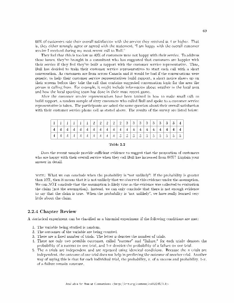
69
60% of customers rate their overall satisfaction with the service they received at 4 or higher. Thatis, they either strongly agree or agreed with the statement, �I am happy with the overall customerservice I received during my most recent call to Bull.�
They feel that this is too low as 40% of customers were not happy with their service. To addressthese issues, they've brought in a consultant who has suggested that customers are happier withtheir service if they feel they've built a rapport with the customer service representative. Thus,Bull has decided to train their customer service representatives to start each call with a shortconversation. As customers are from across Canada and it would be bad if the conversations weregeneric, to help their customer service representatives build rapport, a short notice shows up ontheir screens before they take the call that contains suggested conversation topic for the area theperson is calling from. For example, it might include information about weather in the local areaand how the local sporting team has done in their most recent game.
After the customer service representatives have been trained in how to make small talk tobuild rapport, a random sample of sixty customers who called Bull and spoke to a customer servicerepresentative is taken. The participants are asked the same question about their overall satisfactionwith their customer service phone call as stated above. The results of the survey are listed below:
1 1 1 1 1 1 2 2 2 2 2 3 3 3 3 3 3 3 3 4
4 4 4 4 4 4 4 4 4 4 4 4 4 4 4 4 4 4 4 4
4 4 4 4 4 4 4 4 4 4 5 5 5 5 5 5 5 5 5 5
Table 2.2
Does the recent sample provide su�cient evidence to suggest that the proportion of customerswho are happy with their overall service when they call Bull has increased from 60%? Explain youranswer in detail.
note: What we can conclude when the probability is �not unlikely�: If the probability is greaterthan 10%, then it means that it is not unlikely that we observed this evidence under the assumption.We can NOT conclude that the assumption is likely true as the evidence was collected to evaluationthe claim (not the assumption). Instead, we can only conclude that there is not enough evidenceto say that the claim is true. When the probability is �not unlikely�, we have really learned verylittle about the claim.
2.2.4 Chapter Review
A statistical experiment can be classi�ed as a binomial experiment if the following conditions are met:
1. The variable being studied is random.2. The outcomes of the variable are being counted.3. There are a �xed number of trials. The letter n denotes the number of trials.4. There are only two possible outcomes, called "success" and "failure," for each trialπ denotes the
probability of a success on one trial, and 1-π denotes the probability of a failure on one trial.5. The n trials are independent and are repeated using identical conditions. Because the n trials are
independent, the outcome of one trial does not help in predicting the outcome of another trial. Anotherway of saying this is that for each individual trial, the probability, π, of a success and probability, 1-π,of a failure remain constant.
Available for free at Connexions <http://cnx.org/content/col12245/1.3>
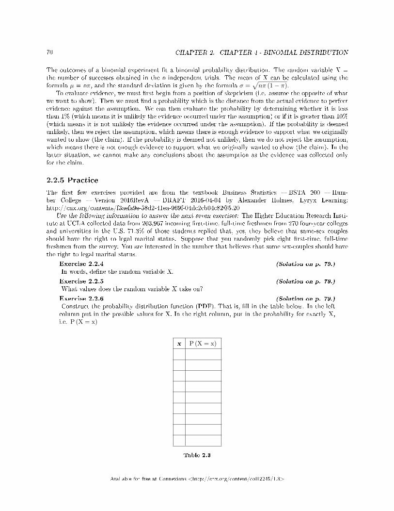
70 CHAPTER 2. CHAPTER 4 - BINOMIAL DISTRIBUTION
The outcomes of a binomial experiment �t a binomial probability distribution. The random variable X =the number of successes obtained in the n independent trials. The mean of X can be calculated using theformula µ = nπ, and the standard deviation is given by the formula σ =
√nπ (1− π).
To evaluate evidence, we must �rst begin from a position of skepticism (i.e. assume the opposite of whatwe want to show). Then we must �nd a probability which is the distance from the actual evidence to perfectevidence against the assumption. We can then evaluate the probability by determining whether it is lessthan 1% (which means it is unlikely the evidence occurred under the assumption) or if it is greater than 10%(which means it is not unlikely the evidence occurred under the assumption). If the probability is deemedunlikely, then we reject the assumption, which means there is enough evidence to support what we originallywanted to show (the claim). If the probability is deemed not unlikely, then we do not reject the assumption,which means there is not enough evidence to support what we originally wanted to show (the claim). In thelatter situation, we cannot make any conclusions about the assumption as the evidence was collected onlyfor the claim.
2.2.5 Practice
The �rst few exercises provided are from the textbook Business Statistics � BSTA 200 � Hum-ber College � Version 2016RevA � DRAFT 2016-04-04 by Alexander Holmes, Lyryx Learning:http://cnx.org/contents/[email protected]
Use the following information to answer the next seven exercises: The Higher Education Research Insti-tute at UCLA collected data from 203,967 incoming �rst-time, full-time freshmen from 270 four-year collegesand universities in the U.S. 71.3% of those students replied that, yes, they believe that same-sex couplesshould have the right to legal marital status. Suppose that you randomly pick eight �rst-time, full-timefreshmen from the survey. You are interested in the number that believes that same sex-couples should havethe right to legal marital status.
Exercise 2.2.4 (Solution on p. 79.)
In words, de�ne the random variable X.
Exercise 2.2.5 (Solution on p. 79.)
What values does the random variable X take on?
Exercise 2.2.6 (Solution on p. 79.)
Construct the probability distribution function (PDF). That is, �ll in the table below. In the leftcolumn put in the possible values for X. In the right column, put in the probability for exactly X,i.e. P (X = x)
x P (X = x)
Table 2.3
Available for free at Connexions <http://cnx.org/content/col12245/1.3>

71
Exercise 2.2.7 (Solution on p. 80.)
On average (µ), how many would you expect to answer yes?
Exercise 2.2.8 (Solution on p. 80.)
What is the standard deviation (σ)?
Exercise 2.2.9 (Solution on p. 80.)
What is the probability that at most �ve of the freshmen reply �yes�?
Exercise 2.2.10 (Solution on p. 80.)
What is the probability that at least two of the freshmen reply �yes�?
Exercise 2.2.11 (Solution on p. 80.)
A school newspaper reporter decides to randomly survey 12 students to see if they will attend Tet(Vietnamese New Year) festivities this year. Based on past years, she knows that 18% of studentsattend Tet festivities. We are interested in the number of students who will attend the festivities.
a. In words, de�ne the random variable X.b. List the values that X may take on.c. How many of the 12 students do we expect to attend the festivities?d. Find the probability that at most four students will attend.e. Find the probability that more than two students will attend.
Use the following information to answer the next three multiple choice questions: The probability that theCalgary Flames will win any given game is 0.4617 based on a 45-year win history of 1,616 wins out of 3,500games played (as of Sept. 2017). An upcoming monthly schedule contains 12 games.
Exercise 2.2.12 (Solution on p. 80.)
The expected number of wins for that upcoming month is:
a. 1.67b. 12c. 1616
3500d. 5.54
Let X = the number of games won in that upcoming month.
Exercise 2.2.13 (Solution on p. 80.)
What is the probability that the Calgary Flames win exactly six games in that upcoming month?
a. 0.2178b. 0.4167c. 0.7664d. 0.7116
Exercise 2.2.14 (Solution on p. 80.)
What is the probability that the Calgary Flames win at least �ve games in that upcoming month
a. 0.2176b. 0.2762c. 0.7238d. 0.5062
Exercise 2.2.15 (Solution on p. 80.)
The chance of an Canadian Revenue Agency audit for a tax return with over $25,000 in income isabout 2% per year. We are interested in the expected number of audits a person with that incomehas in a 20-year period. Assume each year is independent.
Available for free at Connexions <http://cnx.org/content/col12245/1.3>
72 CHAPTER 2. CHAPTER 4 - BINOMIAL DISTRIBUTION
a. In words, de�ne the random variable X.b. List the values that X may take on.c. How many audits are expected in a 20-year period?d. Find the probability that a person is not audited at all.e. Find the probability that a person is audited more than twice.
Exercise 2.2.16 (Solution on p. 80.)
According to The World Bank, only 9% of the population of Uganda had access to electricity asof 2009. Suppose we randomly sample 150 people in Uganda. Let X = the number of people whohave access to electricity.
a. Calculate the mean and standard deviation of X.b. Find the probability that 15 people in the sample have access to electricity.c. Find the probability that at most ten people in the sample have access to electricity.d. Find the probability that more than 25 people in the sample have access to electricity.
Exercise 2.2.17 (Solution on p. 81.)
Jenna and Megan looked at the new packaging.�I guess it looks ok.� Megan hedged.�The design team says that this new packaging really sells the time-saving nature of the kit.��But it's kinda o�-putting.� They continued to stare at the new packaging. Jenna and Megan
had developed a make-up kit called `5 minute make-up', which was aimed at women on the go whowanted to put `their face on' but a lot quicker than they usually did. Their target market was newmoms, moms with full-time jobs, full-time students working full-time, . . .. In other words, anyonewho didn't have 30 minutes every morning to do their make-up. Their little start-up was doingwell. They'd arranged for their product to be produced, had made how-to videos on YouTube, andwere starting to get their products put into stores. Their dream placement was in Sephora.
Now that they were more established, they had decided to hire a marketing expert who couldhelp take them to the next level. The �rst thing that Leticia suggested was to change the packaging.She argued that their old packaging didn't convey the premise of the product clearly enough. Withthe help of a design team, Leticia had come up with a packaging that showed a harried womanwith hair everywhere and bags under her eyes looking overwhelmed. But when you �ip the packageover, the woman was now perfectly put together � `only �ve-minute make-up can save you frombeing a hot mess'.
Jenna �nally broke the silence. �I don't know if I would even pick up this package. It just looksso depressing. But what do we do?�
�Leticia wants to put the product in this new packaging in �ve stores that carry our products.Based o� of previous sales numbers, we know that the stores sell 68% of the product we give themin a two-week period.�
�How does that help us? Do we just watch our sales plummet?� Jenna was sounding exasperated.�I'm getting to that.� Megan soothed. �Leticia is convinced this packaging will increase sales.
But what if we can show her that it doesn't? Let's put this packaging into the �ve stores and thensee how many kits were actually sold. I bet that we can show her that the sales went down.�
�I don't see how that is useful. We still have to pay her stupid fee.��You should read her contract more closely. She only gets paid if she can show that sales
increased. If they don't, then not only does she not get paid but she also has to pay for anycontractors (i.e. the design team).�
Jenna perked up visibly at this.Over the next two weeks, �ve stores carried the new packaging. Megan and Jenna provided
each store with 100 kits. At the end of the two weeks, 306 of the kits were sold.
1. What is the observation unit? What is the variable? Categorize it.
Available for free at Connexions <http://cnx.org/content/col12245/1.3>

73
2. What do Jenna and Megan want to show?3. What assumption do Jenna and Megan need to make in order to investigate your answer in
question 2? Write your answer both as a sentence and as a probability.4. What is the evidence that Jenna and Megan have found?5. Describe the process that Jenna and Megan will go through to evaluate this evidence. Your
description should include (but is not limited to) what probability they will �nd and whatthey will do with that probability once they've found it. Don't actually do the process (thatcomes later). Just describe what they will do.
6. Jenna and Megan believe that the binomial distribution will be the best model to �nd therequired probability. Does this situation meet the criteria for a binomial? Examine eachcriterion and comment on whether it is satis�ed here or not.
7. Regardless of your answer above, use a binomial distribution to model this situation. Findthe appropriate probability to evaluate the evidence using MegaStat.
8. In sentence form, explain what the probability you have found means in the context of thequestion. Do not make a conclusion yet. Instead explain what it is a probability of.
9. Now make a conclusion. In particular, answer this question: Is their enough evidence tosuggest that Leticia's new packaging has reduced sales? Justify your answer.
Exercise 2.2.18 (Solution on p. 81.)
Striking Donkey Co�ee recently sold an 80% stake in their company to Baravalle, an Italian co�eeconglomerate. Striking Donkey's logo is simplistic. Baravalle wants to maintain brand recognition,but also wants to put their stamp on the company. In particular, Baravalle is known for its modernand stylish advertisements.
Designers and marketers at Baravalle have worked tirelessly for the last month to come up withtwo revised Striking Donkey logos (not included, because it is top secret). They are referred to asLogo 1 and Logo 2.
Now they want to determine whether customers show any preference to either logo. To do this,they asked a random sample of 40 customers who were familiar with the Striking Donkey Brandwhich logo they prefer. Participants had to make a choice between the logos.
The results of the study were that 26 out of the 40 participants preferred Logo 2.The marketers at Baravalle now want to do a statistical analysis to determine whether Logo 2
is preferred signi�cantly more than Logo 1.
1. What assumption do you need to start with when determining whether Logo 2 is preferredsigni�cantly more than Logo 1? State your answer both in a sentence and mathematically.
2. Can this situation be modelled by the binomial distribution? Support your answer by showingwhy or why not this situation satis�es each of the �ve criteria of the binomial distribution.
3. After previous issues with horrible new logo launches, Baravalle only wants to go forwardif there is clear evidence that Logo 2 is preferred. Based on this, what level of signi�canceshould they use? Explain your reasoning.
4. Regardless of your answer in b, assume that this situation satis�es the binomial distribution forthe remainder of the question. Use a computer program to �nd that appropriate probabilitythat will allow you to evaluate the evidence.
5. In sentence form, explain what the probability you have found means in the context of thequestion. Do not make a conclusion yet. Instead explain what it is a probability of.
6. Based on the probability, determine whether Logo 2 is preferred signi�cantly more than Logo1. Explain your reasoning.
Available for free at Connexions <http://cnx.org/content/col12245/1.3>
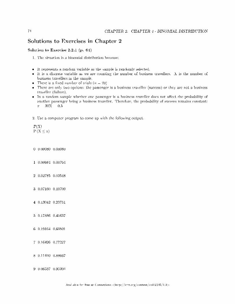
74 CHAPTER 2. CHAPTER 4 - BINOMIAL DISTRIBUTION
Solutions to Exercises in Chapter 2
Solution to Exercise 2.2.1 (p. 64)
1. The situation is a binomial distribution because:
• It represents a random variable as the sample is randomly selected.• It is a discrete variable as we are counting the number of business travellers. X is the number of
business travellers in the sample.• There is a �xed number of trials (n = 20)• There are only two options: the passenger is a business traveller (success) or they are not a business
traveller (failure).• In a random sample whether one passenger is a business traveller does not a�ect the probability of
another passenger being a business traveller. Therefore, the probability of success remains constant:π = 30% = 0.3
2. Use a computer program to come up with the following output.
P(X)P (X ≤ x)
0 0.00080 0.00080
1 0.00684 0.00764
2 0.02785 0.03548
3 0.07160 0.10709
4 0.13042 0.23751
5 0.17886 0.41637
6 0.19164 0.60801
7 0.16426 0.77227
8 0.11440 0.88667
9 0.06537 0.95204
Available for free at Connexions <http://cnx.org/content/col12245/1.3>

75
10 0.03082 0.98286
11 0.01201 0.99486
12 0.00386 0.99872
13 0.00102 0.99974
14 0.00022 0.99996
15 0.00004 0.99999
16 0.00001 1.00000
17 0.00000 1.00000
18 0.00000 1.00000
19 0.00000 1.00000
20 0.00000 1.00000
P(X)P (X ≤ x)
0 0.00080 0.00080
1 0.00684 0.00764
2 0.02785 0.03548
3 0.07160 0.10709
4 0.13042 0.23751
Available for free at Connexions <http://cnx.org/content/col12245/1.3>

76 CHAPTER 2. CHAPTER 4 - BINOMIAL DISTRIBUTION
5 0.17886 0.41637
6 0.19164 0.60801
7 0.16426 0.77227
8 0.11440 0.88667
9 0.06537 0.95204
10 0.03082 0.98286
11 0.01201 0.99486
12 0.00386 0.99872
13 0.00102 0.99974
14 0.00022 0.99996
15 0.00004 0.99999
16 0.00001 1.00000
17 0.00000 1.00000
18 0.00000 1.00000
19 0.00000 1.00000
20 0.00000 1.00000
P(X)P (X ≤ x)
Available for free at Connexions <http://cnx.org/content/col12245/1.3>

77
0 0.00080 0.00080
1 0.00684 0.00764
2 0.02785 0.03548
3 0.07160 0.10709
4 0.13042 0.23751
5 0.17886 0.41637
6 0.19164 0.60801
7 0.16426 0.77227
8 0.11440 0.88667
9 0.06537 0.95204
10 0.03082 0.98286
11 0.01201 0.99486
12 0.00386 0.99872
13 0.00102 0.99974
14 0.00022 0.99996
15 0.00004 0.99999
16 0.00001 1.00000
Available for free at Connexions <http://cnx.org/content/col12245/1.3>
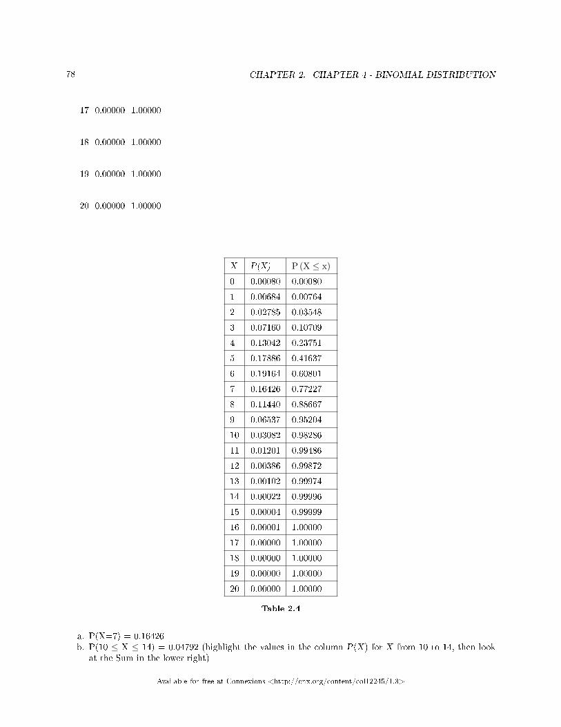
78 CHAPTER 2. CHAPTER 4 - BINOMIAL DISTRIBUTION
17 0.00000 1.00000
18 0.00000 1.00000
19 0.00000 1.00000
20 0.00000 1.00000
X P(X) P (X ≤ x)
0 0.00080 0.00080
1 0.00684 0.00764
2 0.02785 0.03548
3 0.07160 0.10709
4 0.13042 0.23751
5 0.17886 0.41637
6 0.19164 0.60801
7 0.16426 0.77227
8 0.11440 0.88667
9 0.06537 0.95204
10 0.03082 0.98286
11 0.01201 0.99486
12 0.00386 0.99872
13 0.00102 0.99974
14 0.00022 0.99996
15 0.00004 0.99999
16 0.00001 1.00000
17 0.00000 1.00000
18 0.00000 1.00000
19 0.00000 1.00000
20 0.00000 1.00000
Table 2.4
a. P(X=7) = 0.16426b. P(10 ≤ X ≤ 14) = 0.04792 (highlight the values in the column P(X) for X from 10 to 14, then look
at the Sum in the lower right)
Available for free at Connexions <http://cnx.org/content/col12245/1.3>
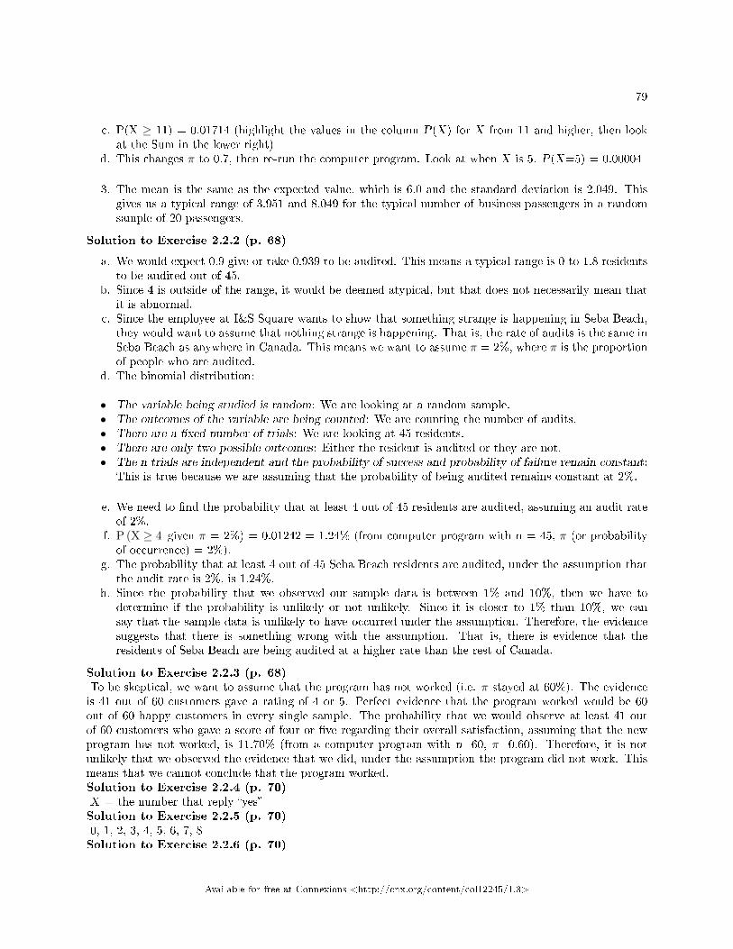
79
c. P(X ≥ 11) = 0.01714 (highlight the values in the column P(X) for X from 11 and higher, then lookat the Sum in the lower right)
d. This changes π to 0.7, then re-run the computer program. Look at when X is 5. P(X=5) = 0.00004
3. The mean is the same as the expected value, which is 6.0 and the standard deviation is 2.049. Thisgives us a typical range of 3.951 and 8.049 for the typical number of business passengers in a randomsample of 20 passengers.
Solution to Exercise 2.2.2 (p. 68)
a. We would expect 0.9 give or take 0.939 to be audited. This means a typical range is 0 to 1.8 residentsto be audited out of 45.
b. Since 4 is outside of the range, it would be deemed atypical, but that does not necessarily mean thatit is abnormal.
c. Since the employee at I&S Square wants to show that something strange is happening in Seba Beach,they would want to assume that nothing strange is happening. That is, the rate of audits is the same inSeba Beach as anywhere in Canada. This means we want to assume π = 2%, where π is the proportionof people who are audited.
d. The binomial distribution:
• The variable being studied is random: We are looking at a random sample.• The outcomes of the variable are being counted: We are counting the number of audits.• There are a �xed number of trials: We are looking at 45 residents.• There are only two possible outcomes: Either the resident is audited or they are not.• The n trials are independent and the probability of success and probability of failure remain constant:
This is true because we are assuming that the probability of being audited remains constant at 2%.
e. We need to �nd the probability that at least 4 out of 45 residents are audited, assuming an audit rateof 2%.
f. P (X ≥ 4 given π = 2%) = 0.01242 = 1.24% (from computer program with n = 45, π (or probabilityof occurrence) = 2%).
g. The probability that at least 4 out of 45 Seba Beach residents are audited, under the assumption thatthe audit rate is 2%, is 1.24%.
h. Since the probability that we observed our sample data is between 1% and 10%, then we have todetermine if the probability is unlikely or not unlikely. Since it is closer to 1% than 10%, we cansay that the sample data is unlikely to have occurred under the assumption. Therefore, the evidencesuggests that there is something wrong with the assumption. That is, there is evidence that theresidents of Seba Beach are being audited at a higher rate than the rest of Canada.
Solution to Exercise 2.2.3 (p. 68)To be skeptical, we want to assume that the program has not worked (i.e. π stayed at 60%). The evidenceis 41 out of 60 customers gave a rating of 4 or 5. Perfect evidence that the program worked would be 60out of 60 happy customers in every single sample. The probability that we would observe at least 41 outof 60 customers who gave a score of four or �ve regarding their overall satisfaction, assuming that the newprogram has not worked, is 11.70% (from a computer program with n=60, π=0.60). Therefore, it is notunlikely that we observed the evidence that we did, under the assumption the program did not work. Thismeans that we cannot conclude that the program worked.Solution to Exercise 2.2.4 (p. 70)X = the number that reply �yes�Solution to Exercise 2.2.5 (p. 70)0, 1, 2, 3, 4, 5, 6, 7, 8Solution to Exercise 2.2.6 (p. 70)
Available for free at Connexions <http://cnx.org/content/col12245/1.3>
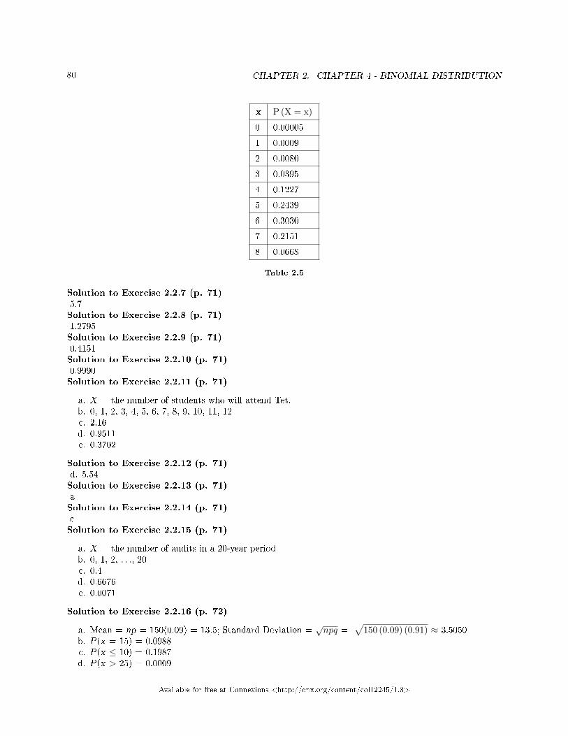
80 CHAPTER 2. CHAPTER 4 - BINOMIAL DISTRIBUTION
x P (X = x)
0 0.00005
1 0.0009
2 0.0080
3 0.0395
4 0.1227
5 0.2439
6 0.3030
7 0.2151
8 0.0668
Table 2.5
Solution to Exercise 2.2.7 (p. 71)5.7Solution to Exercise 2.2.8 (p. 71)1.2795Solution to Exercise 2.2.9 (p. 71)0.4151Solution to Exercise 2.2.10 (p. 71)0.9990Solution to Exercise 2.2.11 (p. 71)
a. X = the number of students who will attend Tet.b. 0, 1, 2, 3, 4, 5, 6, 7, 8, 9, 10, 11, 12c. 2.16d. 0.9511e. 0.3702
Solution to Exercise 2.2.12 (p. 71)d. 5.54Solution to Exercise 2.2.13 (p. 71)aSolution to Exercise 2.2.14 (p. 71)cSolution to Exercise 2.2.15 (p. 71)
a. X = the number of audits in a 20-year periodb. 0, 1, 2, . . ., 20c. 0.4d. 0.6676e. 0.0071
Solution to Exercise 2.2.16 (p. 72)
a. Mean = np = 150(0.09) = 13.5; Standard Deviation =√npq =
√150 (0.09) (0.91) ≈ 3.5050
b. P(x = 15) = 0.0988c. P(x ≤ 10) = 0.1987d. P(x > 25) = 0.0009
Available for free at Connexions <http://cnx.org/content/col12245/1.3>
81
Solution to Exercise 2.2.17 (p. 72)
1. Observational unit: Five-minute make-up kit; Variable: Did it sell or not; Categorize: Categorical2. They want to show that the new packaging will decrease sales.3. They need to assume the opposite of what they want to show. Therefore, they need to assume that the
new packaging does not decrease sales. Therefore, the proportion of kits sold stays the same at 68%.4. They have found that out of 500 kits supplied, 306 of them have been sold.5. They �rst need to start with an assumption ( = 68%). Then they need to come up with a model based
on this assumption. Once they have the model, they will use it to �nd the probability that the storessold at most 306 out of 500 kits, assuming that the new packaging has not decreased sales (i.e. stayedat 68%). Once they have the probability, they need to determine whether the event is likely or unlikely.An event is unlikely if the probability is less than 1%. An event is likely if the probability is morethan 10%. If the event is unlikely, then it means that it is unlikely we observed the evidence under theassumption. Since we know the evidence actually happened, that makes us question the assumption.Thus, it is unlikely the assumption is true based o� of the evidence. If the event is likely to happen,then the assumption is likely to be true based o� of the evidence.
6. • Is the data randomly collected? Most likely not. The 500 kits that we are looking at were notrandomly selected.
• Is the data discrete (countable)? As we are counting the number of kits that are sold the data isdiscrete.
• Are the events independent? This may be a fair assumption for this study. Most likely the saleof one kit is not dependent on whether another kit is sold. Though if two friends buy the kitstogether or someone buys a bunch as presents, this is not the case, but in general it is more likelyindependent than dependent.
• Are there a �xed number of trials? In this case, the number of trials would be the 500 kits withthe new packaging.
• Are there two possible outcomes? Either a kit is sold or it is not.7. P (X ≤ 36) = 0.00077 = 0.077%8. The probability that we observed at most 306 out of 500 kits sold (1), assuming the rate of sales is
68%, is 0.077%9. Since the probability is less than 1%, then it is very unlikely that we would have observed this evidence
under the assumption. Since we actually observed the evidence but assumed that the rate was 68%,what we have assumed is called into question. Therefore, it is unlikely that the assumption is true .Therefore, it is likely that the new packaging has resulted in a decrease in sales .
Solution to Exercise 2.2.18 (p. 73)Observational unit: People who are familiar with Striking Donkey Co�ee; Variable: Whether they preferLogo 2; Type of variable: Categorical.
1. They need to assume the opposite of what they want to show. This means they need to assume thatLogo 2 is NOT preferred signi�cantly more than Logo 1. This would mean they are preferred equally.Therefore, there is a 50% chance that someone will choose Logo 2.
2. • The data is collected randomly: Yes. It is a random sample of participants.• The outcomes are counted: Yes. They count how many people like Logo 2.• There are two possible outcomes: Yes. Either they prefer Logo 2 or they did not.• There are a �xed number of trials: Yes. They asked 40 people.• The trials are independent of each other. Yes. It is fair to assume that no participant's preference
is based on another participants preference.3. The more unlikely it is that we observed our evidence, the smaller the probability will be. This means,
the smaller the probability, the more unlikely it is that the assumption (i.e. that there is no preferencebetween the logos) is true. Since the marketers want clear evidence that there is a preference, theywant a smaller probability, which would show it is unlikely that there is a preference between the logos.The level of signi�cance is the threshold between likely and unlikely. Thus, if they want clear evidence,
Available for free at Connexions <http://cnx.org/content/col12245/1.3>
82 CHAPTER 2. CHAPTER 4 - BINOMIAL DISTRIBUTION
they want to set their threshold �high�, meaning they want to make it a small number. Since the levelof signi�cance is between 1% and 10%, the lowest level of signi�cance (meaning the highest thresholdof evidence) is at 1%.
4. P (X ≥ 26) = 0.04035 = 4.04%5. The probability that we observed at least 26 out of 40 people who preferred Logo 2, assuming that
there was no preference between the logos, is 4.04%.6. Since the probability is greater than 1% (it is 4.04%), it is not unlikely that we observed at least
26 out of 40 people who preferred Logo 2, assuming that there was no preference between the logos.Therefore, we do not reject that there was no preference between the logos. This suggests that Logo 2is NOT preferred signi�cantly more than Logo 1.
Available for free at Connexions <http://cnx.org/content/col12245/1.3>
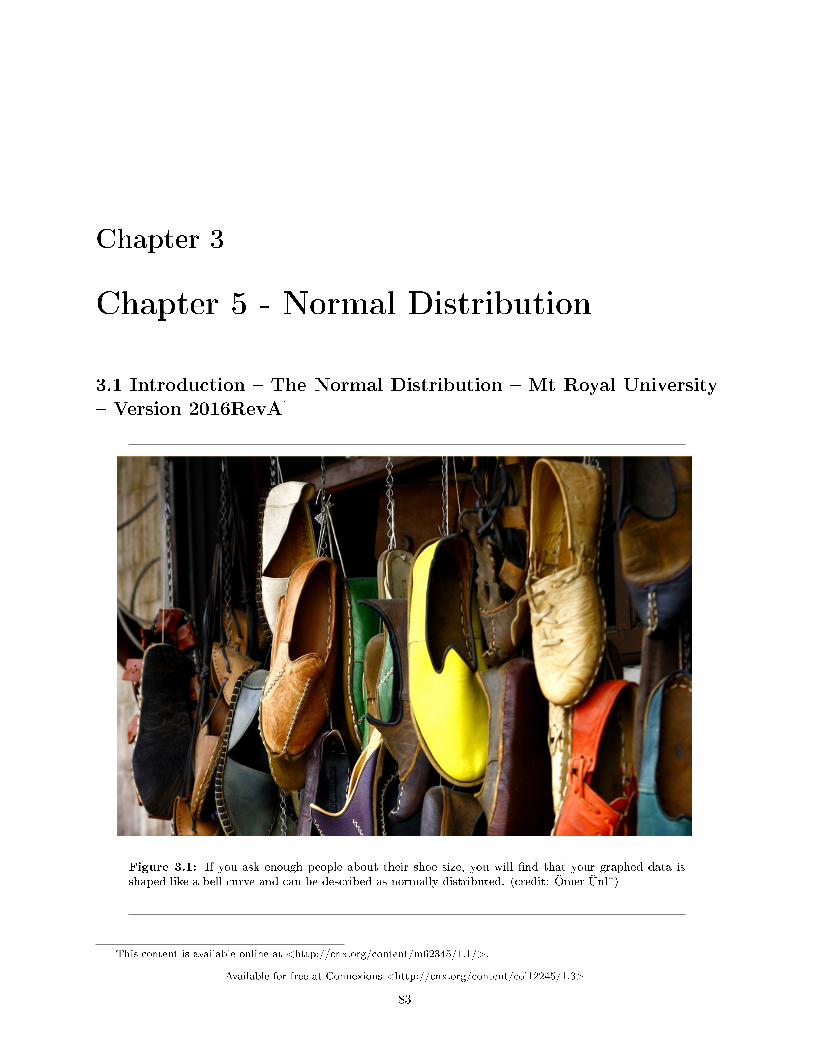
Chapter 3
Chapter 5 - Normal Distribution
3.1 Introduction � The Normal Distribution � Mt Royal University� Version 2016RevA1
Figure 3.1: If you ask enough people about their shoe size, you will �nd that your graphed data isshaped like a bell curve and can be described as normally distributed. (credit: Ömer Ünl�)
1This content is available online at <http://cnx.org/content/m62345/1.1/>.
Available for free at Connexions <http://cnx.org/content/col12245/1.3>
83
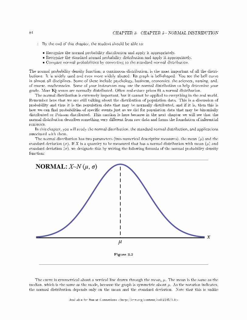
84 CHAPTER 3. CHAPTER 5 - NORMAL DISTRIBUTION
: By the end of this chapter, the student should be able to:
• Recognize the normal probability distribution and apply it appropriately.• Recognize the standard normal probability distribution and apply it appropriately.• Compare normal probabilities by converting to the standard normal distribution.
The normal probability density function, a continuous distribution, is the most important of all the distri-butions. It is widely used and even more widely abused. Its graph is bell-shaped. You see the bell curvein almost all disciplines. Some of these include psychology, business, economics, the sciences, nursing, and,of course, mathematics. Some of your instructors may use the normal distribution to help determine yourgrade. Most IQ scores are normally distributed. Often real-estate prices �t a normal distribution.
The normal distribution is extremely important, but it cannot be applied to everything in the real world.Remember here that we are still talking about the distribution of population data. This is a discussion ofprobability and thus it is the population data that may be normally distributed, and if it is, then this ishow we can �nd probabilities of speci�c events just as we did for population data that may be binomiallydistributed or Poisson distributed. This caution is here because in the next chapter we will see that thenormal distribution describes something very di�erent from raw data and forms the foundation of inferentialstatistics.
In this chapter, you will study the normal distribution, the standard normal distribution, and applicationsassociated with them.
The normal distribution has two parameters (two numerical descriptive measures), the mean (µ) and thestandard deviation (σ). If X is a quantity to be measured that has a normal distribution with mean (µ) andstandard deviation (σ), we designate this by writing the following formula of the normal probability densityfunction:
Figure 3.2
The curve is symmetrical about a vertical line drawn through the mean, µ. The mean is the same as themedian, which is the same as the mode, because the graph is symmetric about µ. As the notation indicates,the normal distribution depends only on the mean and the standard deviation. Note that this is unlike
Available for free at Connexions <http://cnx.org/content/col12245/1.3>
85
several probability density functions we have already studied, such as the Poisson, where the mean is equalto µ and the standard deviation simply the square root of the mean, or the binomial, where p is used todetermine both the mean and standard deviation. Since the area under the curve must equal one, a changein the standard deviation, σ, causes a change in the shape of the curve; the curve becomes fatter and wideror skinnier and taller depending on σ. A change in µ causes the graph to shift to the left or right. Thismeans there are an in�nite number of normal probability distributions. One of special interest is called thestandard normal distribution.
3.1.1 Formula Review
X ∼ N(µ, σ)µ = the mean; σ = the standard deviation
3.2 The Standard Normal Distribution� The Normal Distribution�MRU - C Lemieux2
The standard normal distribution is a normal distribution of standardized values called z-scores.A z-score is measured in units of the standard deviation. For example, if the mean of a normaldistribution is �ve and the standard deviation is two, the value x = 11 is three standard deviations above(or to the right of) the mean. The calculation is as follows:
x = µ + (z)(σ) = 5 + (3)(2) = 11The z-score is three.The mean for the standard normal distribution is zero, and the standard deviation is one. What this
does is dramatically simplify the mathematical calculation of probabilities. Take a moment and substitutezero and one in the appropriate places in the above formula and you can see that the equation collapses intoone that can be much more easily solved using integral calculus. The transformation z = x−µ
σ produces thedistribution Z ∼ N(0, 1). The value x comes from a known normal distribution with known mean µ andknown standard deviation σ. The z-score tells how many standard deviations a particular x is away fromthe mean.
3.2.1 Z-Scores
If X is a normally distributed random variable and X ∼ N(µ, σ), then the z-score is:
z =x −− µ
σ(3.2)
The z-score tells you how many standard deviations the value x is above (to the right of) orbelow (to the left of) the mean, µ. Values of x that are larger than the mean have positive z-scores,and values of x that are smaller than the mean have negative z-scores. If x equals the mean, then x has az-score of zero.
Example 3.1Suppose X ∼ N(5, 6). This says that x is a normally distributed random variable with mean µ =5 and standard deviation σ = 6. Suppose x = 17. Then:
z =x−−µσ
=17−−5
6= 2 (3.2)
This means that x = 17 is two standard deviations (2σ) above or to the right of the mean µ =5. The standard deviation is σ = 6.
Now suppose x = 1. Then: z = x−−µσ = 1−−5
6 = �0.67 (rounded to two decimal places)
2This content is available online at <http://cnx.org/content/m64939/1.1/>.
Available for free at Connexions <http://cnx.org/content/col12245/1.3>
86 CHAPTER 3. CHAPTER 5 - NORMAL DISTRIBUTION
This means that x = 1 is 0.67 standard deviations (�0.67σ) below or to the left ofthe mean µ = 5.
Example 3.2Some doctors believe that a person can lose �ve pounds, on average, in a month by reducing his orher fat intake and by exercising consistently. Suppose weight loss has a normal distribution. Let X= the amount of weight lost(in pounds) by a person in a month. Use a standard deviation of twopounds. X ∼ N(5, 2).
ProblemSuppose a person gained three pounds (a negative weight loss). Then z = __________. Thisz-score tells you that x = �3 is ________ standard deviations to the __________ (rightor left) of the mean.
Solution
Z =x− µσ
=−3− 5
2= −4 (3.2)
z = �4. This z-score tells you that x = �3 is four standard deviations to the left of the mean.
Suppose the random variables X and Y have the following normal distributions: X ∼ N(5, 6) and Y ∼ N(2,1). If x = 17, then z = 2. (This was previously shown.) If y = 4, what is z?
z = y−µσ = 4−2
1 = 2 where µ = 2 and σ = 1.The z-score for y = 4 is z = 2. This means that four is z = 2 standard deviations to the right of the
mean. Therefore, x = 17 and y = 4 are both two (of their own) standard deviations to the right of theirrespective means.
The z-score allows us to compare data that are scaled di�erently. To understand the concept,suppose X ∼ N(5, 6) represents weight gains for one group of people who are trying to gain weight in asix week period and Y ∼ N(2, 1) measures the same weight gain for a second group of people. A negativeweight gain would be a weight loss. Since x = 17 and y = 4 are each two standard deviations to the rightof their means, they represent the same, standardized weight gain relative to their means.
:
Exercise 3.2.1 (Solution on p. 102.)
Fill in the blanks.
Jerome averages 16 points a game with a standard deviation of four points. X ∼ N(16,4).Suppose Jerome scores ten points in a game. The z�score when x = 10 is �1.5. This scoretells you that x = 10 is _____ standard deviations to the ______(right or left) ofthe mean______(What is the mean?).
The Empirical RuleIf X is a random variable and has a normal distribution with mean µ and standard deviation σ, then theEmpirical Rule says the following:
• About 68.26% of the x values lie between �1σ and +1σ of the mean µ (within one standard deviationof the mean).
• About 95.44% of the x values lie between �2σ and +2σ of the mean µ (within two standard deviationsof the mean).
Available for free at Connexions <http://cnx.org/content/col12245/1.3>
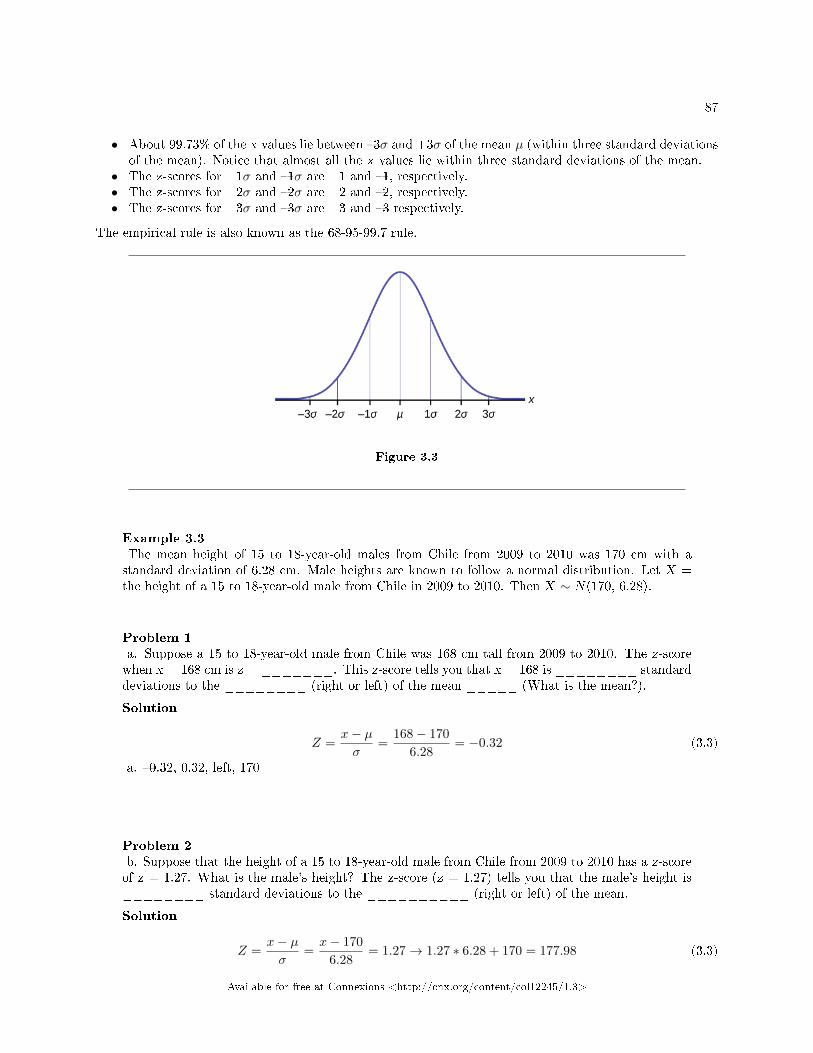
87
• About 99.73% of the x values lie between �3σ and +3σ of the mean µ (within three standard deviationsof the mean). Notice that almost all the x values lie within three standard deviations of the mean.
• The z-scores for +1σ and �1σ are +1 and �1, respectively.• The z-scores for +2σ and �2σ are +2 and �2, respectively.• The z-scores for +3σ and �3σ are +3 and �3 respectively.
The empirical rule is also known as the 68-95-99.7 rule.
Figure 3.3
Example 3.3The mean height of 15 to 18-year-old males from Chile from 2009 to 2010 was 170 cm with astandard deviation of 6.28 cm. Male heights are known to follow a normal distribution. Let X =the height of a 15 to 18-year-old male from Chile in 2009 to 2010. Then X ∼ N(170, 6.28).
Problem 1a. Suppose a 15 to 18-year-old male from Chile was 168 cm tall from 2009 to 2010. The z-scorewhen x = 168 cm is z = _______. This z-score tells you that x = 168 is ________ standarddeviations to the ________ (right or left) of the mean _____ (What is the mean?).
Solution
Z =x− µσ
=168− 170
6.28= −0.32 (3.3)
a. �0.32, 0.32, left, 170
Problem 2b. Suppose that the height of a 15 to 18-year-old male from Chile from 2009 to 2010 has a z-scoreof z = 1.27. What is the male's height? The z-score (z = 1.27) tells you that the male's height is________ standard deviations to the __________ (right or left) of the mean.
Solution
Z =x− µσ
=x− 170
6.28= 1.27→ 1.27 ∗ 6.28 + 170 = 177.98 (3.3)
Available for free at Connexions <http://cnx.org/content/col12245/1.3>
88 CHAPTER 3. CHAPTER 5 - NORMAL DISTRIBUTION
b. 177.98, 1.27, right
:
Exercise 3.2.2 (Solution on p. 102.)
In 2012, 1,664,479 students took the SAT exam. The distribution of scores in the verbalsection of the SAT had a mean µ = 496 and a standard deviation σ = 114. Let X = aSAT exam verbal section score in 2012. Then X ∼ N(496, 114).
Find the z-scores for x1 = 325 and x2 = 366.21. Interpret each z-score. What can yousay about x1 = 325 and x2 = 366.21?
Example 3.4Suppose x has a normal distribution with mean 50 and standard deviation 6.
• About 68% of the x values lie between �1σ = (�1)(6) = �6 and 1σ = (1)(6) = 6 of the mean50. The values 50 � 6 = 44 and 50 + 6 = 56 are within one standard deviation of the mean50. The z-scores are �1 and +1 for 44 and 56, respectively.
• About 95% of the x values lie between �2σ = (�2)(6) = �12 and 2σ = (2)(6) = 12. Thevalues 50 � 12 = 38 and 50 + 12 = 62 are within two standard deviations of the mean 50.The z-scores are �2 and +2 for 38 and 62, respectively.
• About 99.7% of the x values lie between �3σ = (�3)(6) = �18 and 3σ = (3)(6) = 18 of themean 50. The values 50 � 18 = 32 and 50 + 18 = 68 are within three standard deviations ofthe mean 50. The z-scores are �3 and +3 for 32 and 68, respectively.
:
Exercise 3.2.3 (Solution on p. 102.)
Suppose X has a normal distribution with mean 25 and standard deviation �ve. Betweenwhat values of x do 68% of the values lie?
:
Exercise 3.2.4 (Solution on p. 102.)
The scores on a college entrance exam have an approximate normal distribution withmean, µ = 52 points and a standard deviation, σ = 11 points.
a.About 68% of the y values lie between what two values? These values are________________. The z-scores are ________________, respec-tively.
b.About 95% of the y values lie between what two values? These values are________________. The z-scores are ________________, respec-tively.
c.About 99.7% of the y values lie between what two values? These values are________________. The z-scores are ________________, respec-tively.
Available for free at Connexions <http://cnx.org/content/col12245/1.3>
89
3.2.2 References
�Blood Pressure of Males and Females.� StatCruch, 2013. Available online athttp://www.statcrunch.com/5.0/viewreport.php?reportid=11960 (accessed May 14, 2013).
�The Use of Epidemiological Tools in Con�ict-a�ected populations: Open-access educational resources forpolicy-makers: Calculation of z-scores.� London School of Hygiene and Tropical Medicine, 2009. Availableonline at http://con�ict.lshtm.ac.uk/page_125.htm (accessed May 14, 2013).
�2012 College-Bound Seniors Total Group Pro�le Report.� CollegeBoard, 2012. Available online athttp://media.collegeboard.com/digitalServices/pdf/research/TotalGroup-2012.pdf (accessed May 14, 2013).
�Digest of Education Statistics: ACT score average and standard deviations by sex and race/ethnicityand percentage of ACT test takers, by selected composite score ranges and planned �elds of study:Selected years, 1995 through 2009.� National Center for Education Statistics. Available online athttp://nces.ed.gov/programs/digest/d09/tables/dt09_147.asp (accessed May 14, 2013).
Data from the San Jose Mercury News.Data from The World Almanac and Book of Facts.�List of stadiums by capacity.� Wikipedia. Available online at
https://en.wikipedia.org/wiki/List_of_stadiums_by_capacity (accessed May 14, 2013).Data from the National Basketball Association. Available online at www.nba.com (accessed May 14,
2013).
3.2.3 Chapter Review
A z-score is a standardized value. Its distribution is the standard normal, Z ∼ N(0, 1). The mean of thez-scores is zero and the standard deviation is one. If z is the z-score for a value x from the normal distributionN(µ, σ) then z tells you how many standard deviations x is above (greater than) or below (less than) µ.
3.2.4 Practice Questions
Exercise 3.2.5 (Solution on p. 102.)
In a normal distribution, x = 3 and z = 0.67. This tells you that x = 3 is ____ standarddeviations to the ____ (right or left) of the mean.
Exercise 3.2.6 (Solution on p. 102.)
In a normal distribution, x = �5 and z = �3.14. This tells you that x = �5 is ____ standarddeviations to the ____ (right or left) of the mean.
Exercise 3.2.7 (Solution on p. 102.)
About what percent of x values from a normal distribution lie within one standard deviation (leftand right) of the mean of that distribution?
Exercise 3.2.8 (Solution on p. 102.)
About what percent of the x values from a normal distribution lie within two standard deviations(left and right) of the mean of that distribution?
Exercise 3.2.9 (Solution on p. 102.)
About what percent of x values lie between the second and third standard deviations (both sides)?
Use the following information to answer the next two multiple choice exercises: The patient recovery timefrom a particular surgical procedure is normally distributed with a mean of 5.3 days and a standard deviationof 2.1 days.
Exercise 3.2.10 (Solution on p. 102.)
What is the median recovery time?
a. 2.7b. 5.3c. 7.4
Available for free at Connexions <http://cnx.org/content/col12245/1.3>
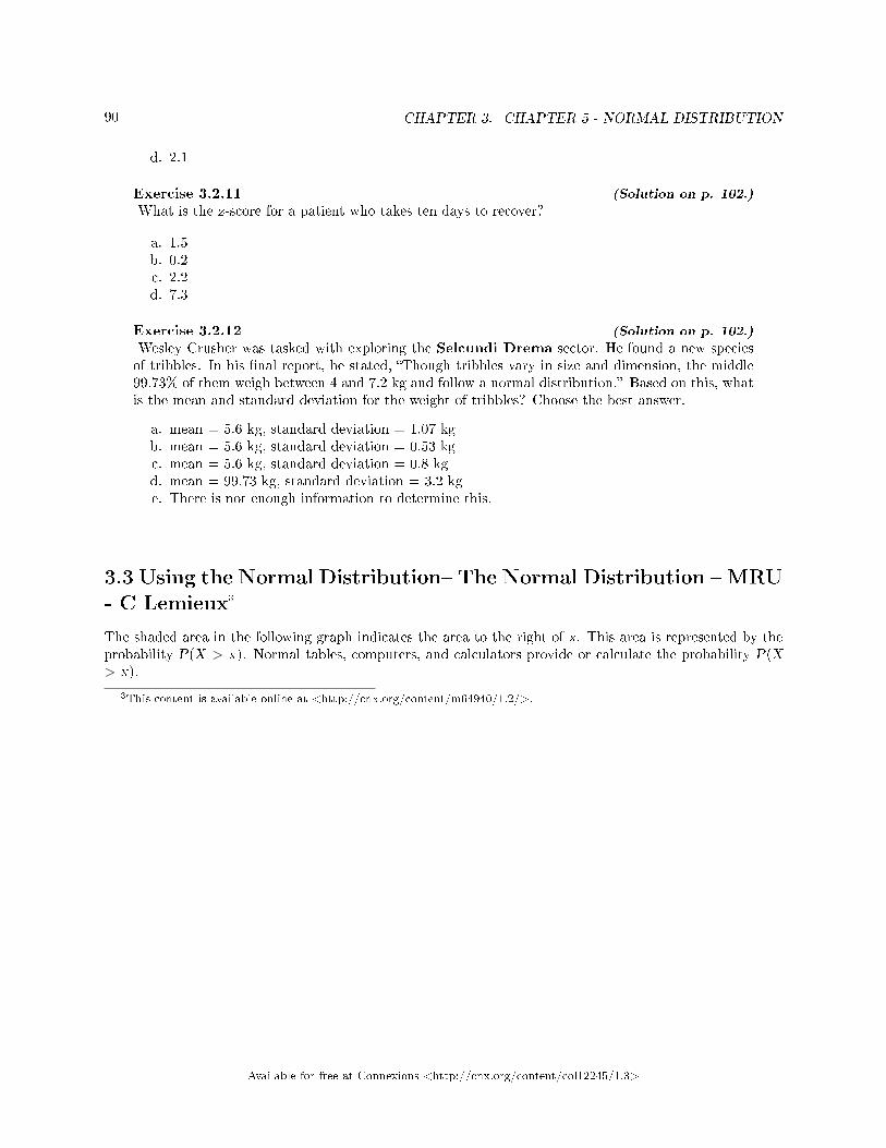
90 CHAPTER 3. CHAPTER 5 - NORMAL DISTRIBUTION
d. 2.1
Exercise 3.2.11 (Solution on p. 102.)
What is the z-score for a patient who takes ten days to recover?
a. 1.5b. 0.2c. 2.2d. 7.3
Exercise 3.2.12 (Solution on p. 102.)
Wesley Crusher was tasked with exploring the Selcundi Drema sector. He found a new speciesof tribbles. In his �nal report, he stated, �Though tribbles vary in size and dimension, the middle99.73% of them weigh between 4 and 7.2 kg and follow a normal distribution.� Based on this, whatis the mean and standard deviation for the weight of tribbles? Choose the best answer.
a. mean = 5.6 kg, standard deviation = 1.07 kgb. mean = 5.6 kg, standard deviation = 0.53 kgc. mean = 5.6 kg, standard deviation = 0.8 kgd. mean = 99.73 kg, standard deviation = 3.2 kge. There is not enough information to determine this.
3.3 Using the Normal Distribution� The Normal Distribution � MRU- C Lemieux3
The shaded area in the following graph indicates the area to the right of x. This area is represented by theprobability P(X > x). Normal tables, computers, and calculators provide or calculate the probability P(X> x).
3This content is available online at <http://cnx.org/content/m64940/1.2/>.
Available for free at Connexions <http://cnx.org/content/col12245/1.3>
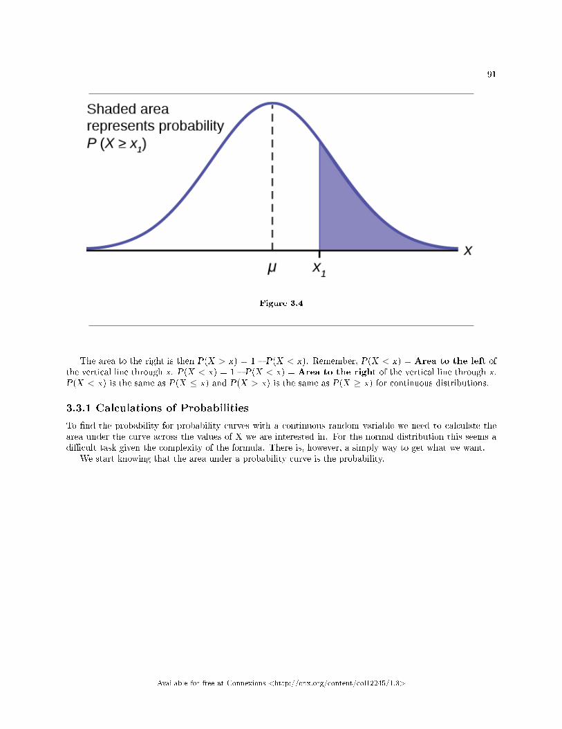
91
Figure 3.4
The area to the right is then P(X > x) = 1 � P(X < x). Remember, P(X < x) = Area to the left ofthe vertical line through x. P(X < x) = 1 � P(X < x) = Area to the right of the vertical line through x.P(X < x) is the same as P(X ≤ x) and P(X > x) is the same as P(X ≥ x) for continuous distributions.
3.3.1 Calculations of Probabilities
To �nd the probability for probability curves with a continuous random variable we need to calculate thearea under the curve across the values of X we are interested in. For the normal distribution this seems adi�cult task given the complexity of the formula. There is, however, a simply way to get what we want.
We start knowing that the area under a probability curve is the probability.
Available for free at Connexions <http://cnx.org/content/col12245/1.3>
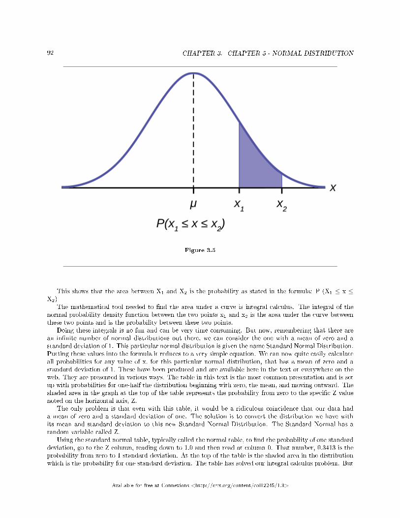
92 CHAPTER 3. CHAPTER 5 - NORMAL DISTRIBUTION
Figure 3.5
This shows that the area between X1 and X2 is the probability as stated in the formula: P (X1 ≤ x ≤X2)
The mathematical tool needed to �nd the area under a curve is integral calculus. The integral of thenormal probability density function between the two points x1 and x2 is the area under the curve betweenthese two points and is the probability between these two points.
Doing these integrals is no fun and can be very time consuming. But now, remembering that there arean in�nite number of normal distributions out there, we can consider the one with a mean of zero and astandard deviation of 1. This particular normal distribution is given the name Standard Normal Distribution.Putting these values into the formula it reduces to a very simple equation. We can now quite easily calculateall probabilities for any value of x, for this particular normal distribution, that has a mean of zero and astandard deviation of 1. These have been produced and are available here in the text or everywhere on theweb. They are presented in various ways. The table in this text is the most common presentation and is setup with probabilities for one-half the distribution beginning with zero, the mean, and moving outward. Theshaded area in the graph at the top of the table represents the probability from zero to the speci�c Z valuenoted on the horizontal axis, Z.
The only problem is that even with this table, it would be a ridiculous coincidence that our data hada mean of zero and a standard deviation of one. The solution is to convert the distribution we have withits mean and standard deviation to this new Standard Normal Distribution. The Standard Normal has arandom variable called Z.
Using the standard normal table, typically called the normal table, to �nd the probability of one standarddeviation, go to the Z column, reading down to 1.0 and then read at column 0. That number, 0.3413 is theprobability from zero to 1 standard deviation. At the top of the table is the shaded area in the distributionwhich is the probability for one standard deviation. The table has solved our integral calculus problem. But
Available for free at Connexions <http://cnx.org/content/col12245/1.3>
93
only if our data has a mean of zero and a standard deviation of 1.However, the essential point here is, the probability for one standard deviation on one normal distribution
is the same on every normal distribution. If the population data set has a mean of 10 and a standard deviationof 5 then the probability from 10 to 15, one standard deviation, is the same as from zero to 1, one standarddeviation on the standard normal distribution. To compute probabilities, areas, for any normal distribution,we need only to convert the particular normal distribution to the standard normal distribution and look upthe answer in the tables. As review, here again is the standardizing formula:
Z =x− µσ
(3.5)
where Z is the value on the standard normal distribution, X is the value from a normal distribution onewishes to convert to the standard normal, µ and σ are, respectively, the mean and standard deviation of thatpopulation. Note that the equation uses µ and σ which denotes population parameters. This is still dealingwith probability so we always are dealing with the population, with known parameter values and a knowndistribution. It is also important to note that because the normal distribution is symmetrical it does notmatter if the z-score is positive or negative when calculating a probability. One standard deviation to theleft (negative Z-score) covers the same area as one standard deviation to the right (positive Z-score). Thisfact is why the Standard Normal tables do not provide areas for the left side of the distribution. Because ofthis symmetry, the Z-score formula is sometimes written as:
Z =|x− µ|σ
(3.5)
Where the vertical lines in the equation means the absolute value of the number.What the standardizing formula is really doing is computing the number of standard deviations X is from
the mean of its own distribution. The standardizing formula and the concept of counting standard deviationsfrom the mean is the secret of all that we will do in this statistics class. The reason this is true is that allof statistics boils down to variation, and the counting of standard deviations is a measure of variation.
This formula, in many disguises, will reappear over and over throughout this course.
Example 3.5The �nal exam scores in a statistics class were normally distributed with a mean of 63 and astandard deviation of �ve.
Problem 1a. Find the probability that a randomly selected student scored more than 65 on the exam.b. Find the probability that a randomly selected student scored less than 85.
Solutiona. Let X = a score on the �nal exam. X ∼ N(63, 5), where µ = 63 and σ = 5
Draw a graph.Then, �nd P(x > 65).P(x > 65) = 0.3446
Available for free at Connexions <http://cnx.org/content/col12245/1.3>
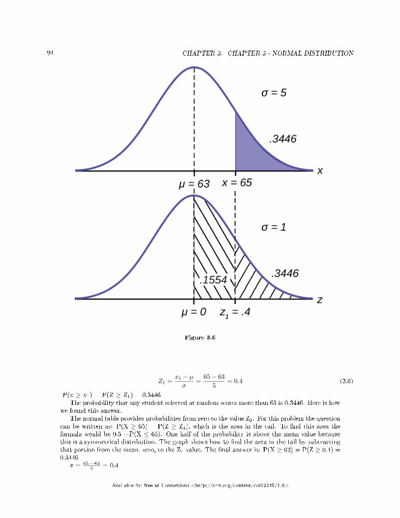
94 CHAPTER 3. CHAPTER 5 - NORMAL DISTRIBUTION
Figure 3.6
Z1 =x1 − µσ
=65− 63
5= 0.4 (3.6)
P(x ≥ x1) = P(Z ≥ Z1) = 0.3446The probability that any student selected at random scores more than 65 is 0.3446. Here is how
we found this answer.The normal table provides probabilities from zero to the value Z1. For this problem the question
can be written as: P(X ≥ 65) = P(Z ≥ Z1), which is the area in the tail. To �nd this area theformula would be 0.5 � P(X ≤ 65). One half of the probability is above the mean value becausethis is a symmetrical distribution. The graph shows how to �nd the area in the tail by subtractingthat portion from the mean, zero, to the Z1 value. The �nal answer is: P(X ≥ 63) = P(Z ≥ 0.4) =0.3446
z = 65 � 635 = 0.4
Available for free at Connexions <http://cnx.org/content/col12245/1.3>
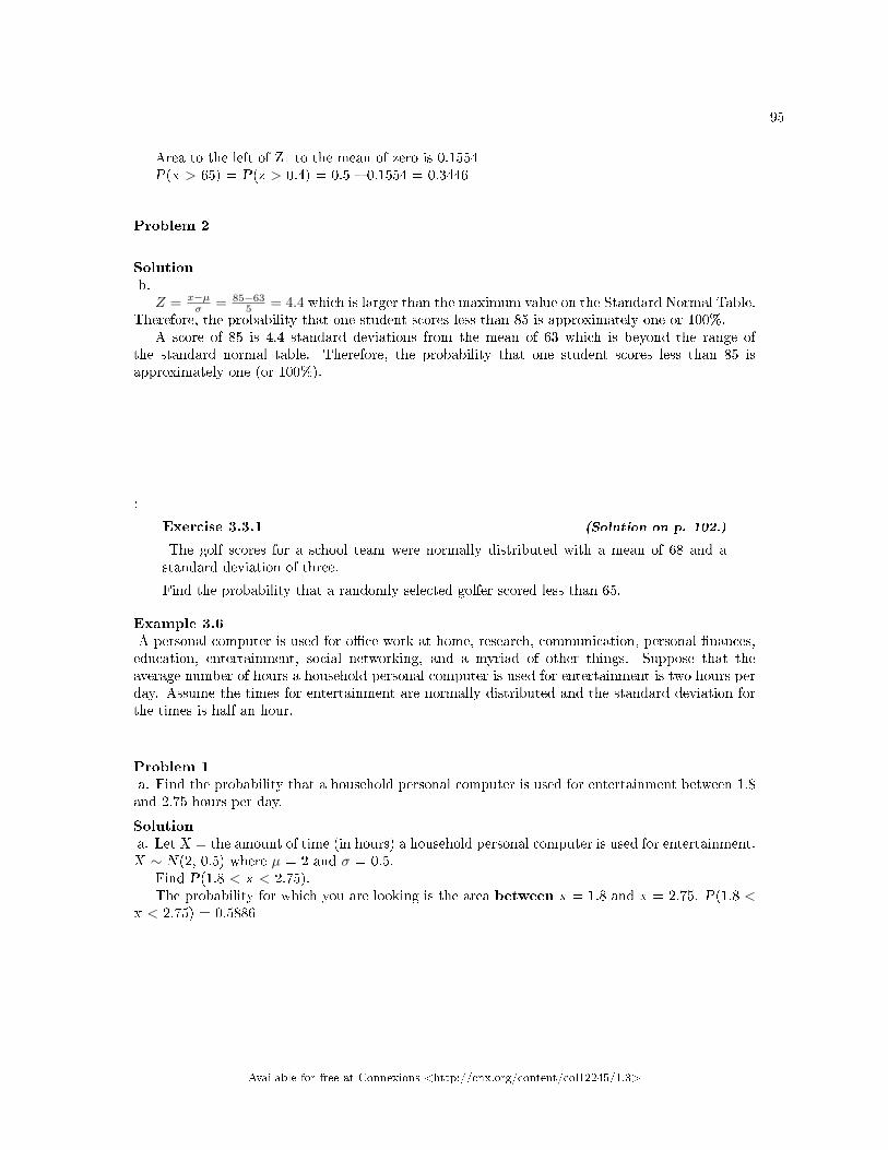
95
Area to the left of Z1 to the mean of zero is 0.1554P(x > 65) = P(z > 0.4) = 0.5 � 0.1554 = 0.3446
Problem 2
Solutionb.Z = x−µ
σ = 85−635 = 4.4 which is larger than the maximum value on the Standard Normal Table.
Therefore, the probability that one student scores less than 85 is approximately one or 100%.A score of 85 is 4.4 standard deviations from the mean of 63 which is beyond the range of
the standard normal table. Therefore, the probability that one student scores less than 85 isapproximately one (or 100%).
:
Exercise 3.3.1 (Solution on p. 102.)
The golf scores for a school team were normally distributed with a mean of 68 and astandard deviation of three.
Find the probability that a randomly selected golfer scored less than 65.
Example 3.6A personal computer is used for o�ce work at home, research, communication, personal �nances,education, entertainment, social networking, and a myriad of other things. Suppose that theaverage number of hours a household personal computer is used for entertainment is two hours perday. Assume the times for entertainment are normally distributed and the standard deviation forthe times is half an hour.
Problem 1a. Find the probability that a household personal computer is used for entertainment between 1.8and 2.75 hours per day.
Solutiona. Let X = the amount of time (in hours) a household personal computer is used for entertainment.X ∼ N(2, 0.5) where µ = 2 and σ = 0.5.
Find P(1.8 < x < 2.75).The probability for which you are looking is the area between x = 1.8 and x = 2.75. P(1.8 <
x < 2.75) = 0.5886
Available for free at Connexions <http://cnx.org/content/col12245/1.3>
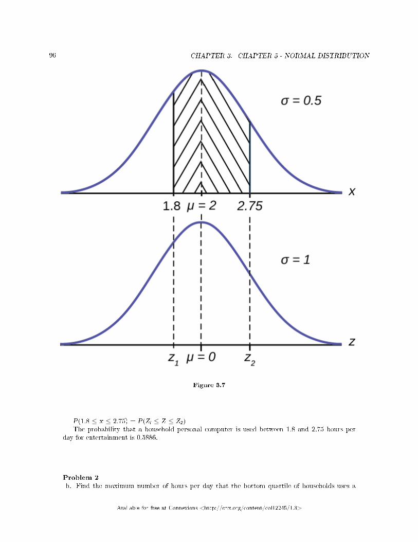
96 CHAPTER 3. CHAPTER 5 - NORMAL DISTRIBUTION
Figure 3.7
P(1.8 ≤ x ≤ 2.75) = P(Zi ≤ Z ≤ Z2)The probability that a household personal computer is used between 1.8 and 2.75 hours per
day for entertainment is 0.5886.
Problem 2b. Find the maximum number of hours per day that the bottom quartile of households uses a
Available for free at Connexions <http://cnx.org/content/col12245/1.3>
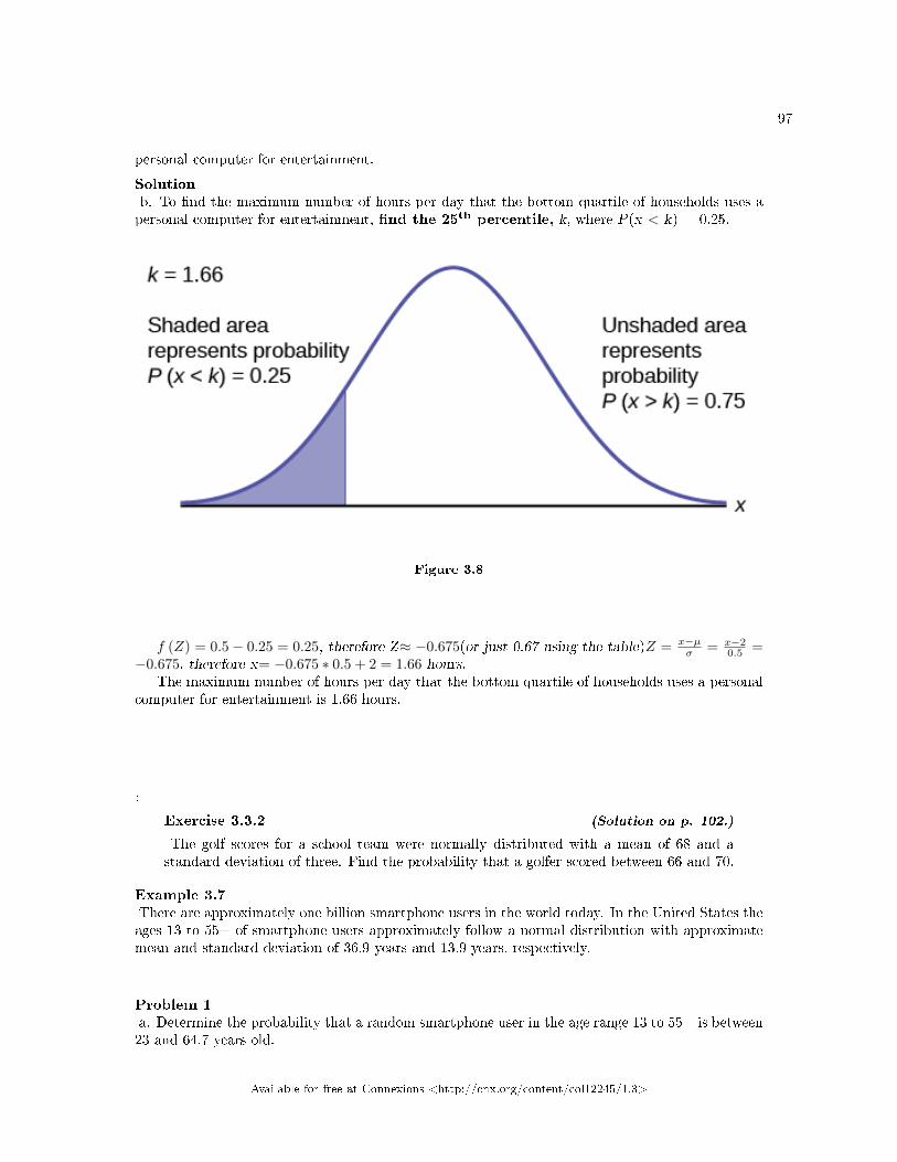
97
personal computer for entertainment.
Solutionb. To �nd the maximum number of hours per day that the bottom quartile of households uses apersonal computer for entertainment, �nd the 25th percentile, k, where P(x < k) = 0.25.
Figure 3.8
f (Z) = 0.5− 0.25 = 0.25, therefore Z≈ −0.675(or just 0.67 using the table)Z = x−µσ = x−2
0.5 =−0.675, therefore x= −0.675 ∗ 0.5 + 2 = 1.66 hours.
The maximum number of hours per day that the bottom quartile of households uses a personalcomputer for entertainment is 1.66 hours.
:
Exercise 3.3.2 (Solution on p. 102.)
The golf scores for a school team were normally distributed with a mean of 68 and astandard deviation of three. Find the probability that a golfer scored between 66 and 70.
Example 3.7There are approximately one billion smartphone users in the world today. In the United States theages 13 to 55+ of smartphone users approximately follow a normal distribution with approximatemean and standard deviation of 36.9 years and 13.9 years, respectively.
Problem 1a. Determine the probability that a random smartphone user in the age range 13 to 55+ is between23 and 64.7 years old.
Available for free at Connexions <http://cnx.org/content/col12245/1.3>

98 CHAPTER 3. CHAPTER 5 - NORMAL DISTRIBUTION
Solutiona. 0.8186
Problem 2b. Determine the probability that a randomly selected smartphone user in the age range 13 to55+ is at most 50.8 years old.
Solutionb. 0.8413
Example 3.8A citrus farmer who grows mandarin oranges �nds that the diameters of mandarin orangesharvested on his farm follow a normal distribution with a mean diameter of 5.85 cm and a standarddeviation of 0.24 cm.
Problem 1a. Find the probability that a randomly selected mandarin orange from this farm has a diameterlarger than 6.0 cm. Sketch the graph.
Solution
Available for free at Connexions <http://cnx.org/content/col12245/1.3>
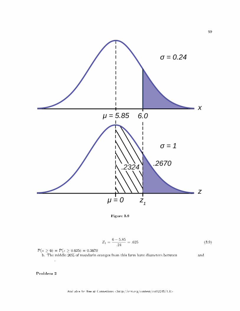
99
Figure 3.9
Z1 =6− 5.85
.24= .625 (3.9)
P(x ≥ 6) = P(z ≥ 0.625) = 0.2670b. The middle 20% of mandarin oranges from this farm have diameters between ______ and
______.
Problem 2
Available for free at Connexions <http://cnx.org/content/col12245/1.3>
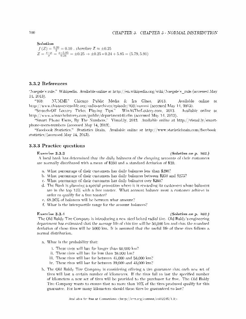
100 CHAPTER 3. CHAPTER 5 - NORMAL DISTRIBUTION
Solutionf (Z) = 0.20
2 = 0.10 , therefore Z ≈ ±0.25Z = x−µ
σ = x−5.850.24 = ±0.25→ ±0.25 ∗ 0.24 + 5.85 = (5.79, 5.91)
3.3.2 References
�Naegele's rule.� Wikipedia. Available online at http://en.wikipedia.org/wiki/Naegele's_rule (accessed May14, 2013).
�403: NUMMI.� Chicago Public Media & Ira Glass, 2013. Available online athttp://www.thisamericanlife.org/radio-archives/episode/403/nummi (accessed May 14, 2013).
�Scratch-O� Lottery Ticket Playing Tips.� WinAtTheLottery.com, 2013. Available online athttp://www.winatthelottery.com/public/department40.cfm (accessed May 14, 2013).
�Smart Phone Users, By The Numbers.� Visual.ly, 2013. Available online at http://visual.ly/smart-phone-users-numbers (accessed May 14, 2013).
�Facebook Statistics.� Statistics Brain. Available online at http://www.statisticbrain.com/facebook-statistics/(accessed May 14, 2013).
3.3.3 Practice questions
Exercise 3.3.3 (Solution on p. 102.)
A local bank has determined that the daily balances of the chequing accounts of their customersare normally distributed with a mean of $280 and a standard deviation of $20.
a. What percentage of their customers has daily balances less than $290?b. What percentage of their customers has daily balances between $250 and $275?c. What percentage of their customers has daily balances over $260?d. The Bank is planning a special promotion where it is rewarding its customers whose balances
are in the top 15% with a free toaster. What account balance must a customer achieve inorder to qualify for a free toaster?
e. 68.26% of balances will be between what amount?f. What is the interquartile range for the account balances?
Exercise 3.3.4 (Solution on p. 102.)
The Old Baldy Tire Company is introducing a new steel belted radial tire. Old Baldy's engineeringdepartment has estimated that the average life of this tire will be 50,000 km and that the standarddeviation of these tires will be 5000 km. It is assumed that the useful life of these tires follows anormal distribution.
a. What is the probability that:
i. These tires will last for longer than 60,000 km?ii. These tires will last for less than 38,000 km?iii. These tires will last for between 45,000 and 58,000 km?iv. These tires will last for between 39,000 and 43,000 km?
b. The Old Baldy Tire Company is considering o�ering a tire guarantee that each new set oftires will last a certain number of kilometers. If the tires fail to last the speci�ed numberof kilometers a new set of tires will be provided to the purchaser for free. The Old BaldyTire Company wants to ensure that no more than 10% of the tires produced qualify for thisguarantee. For how many kilometers should these tires be guaranteed to last?
Available for free at Connexions <http://cnx.org/content/col12245/1.3>

101
c. 35% of tires will last less than how many kilometers?
Available for free at Connexions <http://cnx.org/content/col12245/1.3>

102 CHAPTER 3. CHAPTER 5 - NORMAL DISTRIBUTION
Solutions to Exercises in Chapter 3
to Exercise 3.2.1 (p. 86)1.5, left, 16to Exercise 3.2.2 (p. 88)The z-score for x1 = 325 is z1 = �1.14.
The z-score for x2 = 366.21 is z2 = �1.14.Student 2 scored closer to the mean than Student 1 and, since they both had negative z-scores, Student
2 had the better score.to Exercise 3.2.3 (p. 88)between 20 and 30.to Exercise 3.2.4 (p. 88)
a. About 68% of the values lie between the values 41 and 63. The z-scores are �1 and 1, respectively.b. About 95% of the values lie between the values 30 and 74. The z-scores are �2 and 2, respectively.c. About 99.7% of the values lie between the values 19 and 85. The z-scores are �3 and 3, respectively.
Solution to Exercise 3.2.5 (p. 89)0.67, rightSolution to Exercise 3.2.6 (p. 89)3.14, leftSolution to Exercise 3.2.7 (p. 89)about 68%Solution to Exercise 3.2.8 (p. 89)about 95.44%Solution to Exercise 3.2.9 (p. 89)about 4%Solution to Exercise 3.2.10 (p. 89)bSolution to Exercise 3.2.11 (p. 90)cSolution to Exercise 3.2.12 (p. 90)bto Exercise 3.3.1 (p. 95)normalcdf(1099,65,68,3) = 0.1587to Exercise 3.3.2 (p. 97)normalcdf(66,70,68,3) = 0.4950Solution to Exercise 3.3.3 (p. 100)
a. 0.6915b. 0.3345c. 0.8413d. $300.70e. $260 to $300f. IQR = 293.5-266.5 = $27
Solution to Exercise 3.3.4 (p. 100)
a. i. 0.0228ii. 0.0082iii. 0.7865iv. 0.0669
b. 56407.8 kmc. 48073.4 km
Available for free at Connexions <http://cnx.org/content/col12245/1.3>

Chapter 4
Chapter 6 - Sampling Distribution
4.1 Introduction - Sampling distributions - MRU - C Lemieux1
note: By the end of the chapter, the student should be able to:
• Distinguish between a sample, a population and a sampling distribution.• Know the characteristics of the sampling distribution.• Recognize sampling distribution problems.• Apply and interpret the central limit theorem for both means and proportions.
4.2 Introduction to Sampling Distributions2
When we take a random sample from a population, we expect that there is going to be some variability (i.e.sampling variability) between the information the sample gives us and the whole population. That is, wemight �nd that the sample mean and the population mean are di�erent. We may also �nd that if we takemultiple random samples of size n that the sample mean for each sample is di�erent. The following chapterlooks at how we can better understand the sampling variability in statistics.
Before we go on, here is a reminder of a few terms and symbols.A parameter is a descriptive measure of the population (eg. population mean, population standard
deviation, population proportion).A statistic is a descriptive measure of the sample (eg. sample mean, sample standard deviation, sample
proportion).
Measure Population Sample
Sample size N n
Mean µx−x
Standard deviation σx sx
Proportion π>p
Table 4.1: Table of important symbols
The population mean, population standard deviation, and sample standard deviation have a subscriptof x to demonstrate that they are the measure for the variable X. Though this is mostly notational, it doesbecome important later in this chapter.
1This content is available online at <http://cnx.org/content/m64933/1.1/>.2This content is available online at <http://cnx.org/content/m64932/1.2/>.
Available for free at Connexions <http://cnx.org/content/col12245/1.3>
103
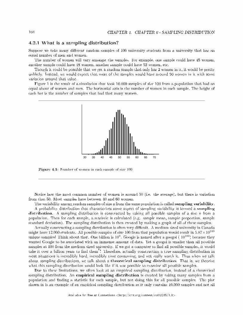
104 CHAPTER 4. CHAPTER 6 - SAMPLING DISTRIBUTION
4.2.1 What is a sampling distribution?
Suppose we take many di�erent random samples of 100 university students from a university that has anequal number of men and women.
The number of women will vary amongst the samples. For example, one sample could have 45 women,another sample could have 48 women, another sample could have 52 women, etc.
Though it could be possible that we get a random sample that only has 2 women in it, it would be prettyunlikely. Instead, we would expect that most of the samples would have around 50 women in it with somevariation around that value.
Figure 1 is the result of a simulation that took 10,000 samples of size 100 from a population that had anequal about of women and men. The horizontal axis is the number of women in each sample. The height ofeach bar is the number of samples that had that many women.
Figure 4.1: Number of women in each sample of size 100
Notice how the most common number of women is around 50 (i.e. the average), but there is variationfrom that 50. Most samples have between 40 and 60 women.
The variability among random samples of size n from the same population is called sampling variability.A probability distribution that characterizes some aspect of sampling variability is termed a sampling
distribution. A sampling distribution is constructed by taking all possible samples of a size n from apopulation. Then for each sample, a statistic is calculated (e.g. sample mean, sample proportion, samplestandard deviation). The sampling distribution is then created by making a graph of all of these samples.
Actually constructing a sampling distribution is often very di�cult. A medium sized university in Canadamight have 12,000 students. All possible samples of size 100 from that population would result in 5.87×10249unique samples! Think about that. One billion is 109. Google is named after a googol ( 10100) because theywanted Google to be associated with an immense amount of data. Yet a googol is smaller than all possiblesamples at 100 from the medium sized university. If we got a computer to �nd all possible samples, it wouldtake it over a billion years to �nd them
3
! Therefore, actually constructing a true sampling distribution inmost situations is incredibly hard, incredibly time consuming, and not really worth it. Thus when we talkabout sampling distributions, we talk about a theoretical sampling distribution. That is, we theorizewhat this sampling distribution would look like if it was possible to examine all possible samples.
Due to these limitations, we often look at an empirical sampling distribution, instead of a theoreticalsampling distribution. An empirical sampling distribution is created by taking many samples from apopulation and �nding a statistic for each sample, but not doing this for all possible samples. The plotshown in is an example of an empirical sampling distribution as it only contains 10,000 samples and not all
Available for free at Connexions <http://cnx.org/content/col12245/1.3>

105
possible samples. The statistic in is the number of women, but we could have also looked at the proportionof women.
In summary, a sampling distribution is a distribution of a statistic. This di�ers from other distributions,like the population distribution, which are distributions for individual data values.
4.2.2 Why do we care about sampling distributions?
Suppose we take a random sample of 100 students from a medium sized university and we �nd that 75 ofthem are women. Does this call into question the assumption that 50% of the students are women? This ishard to �gure out unless we know how likely it is that we could have found this random sample, assumingthat there are an equal number of men and women.
The sampling distribution helps us �nd this probability. From the empirical sampling distribution inFigure 1 we can �nd the probability of getting a random sample of 75 women, assuming that there are anequal number of men and women is 0.0000%. That is, it is really unlikely to get a random sample of 75women out of 100 if there are an equal number of men and women in the population. Based on this, we canbe fairly con�dent that this university probably doesn't have an equal number of men and women. Instead,it is more likely that there are women than men at this university.
The process described above is called inferential statistics. Inferential statistics is used to make aconclusion about the population (all students at the university) from a sample (100 students). In general, todo any form of inferential statistics, we need to use a sampling distribution to either determine how likely orunlikely a statistic is (in hypothesis testing) or to estimate a parameter from a statistic (con�dence intervals).
Thus sampling distributions are the backbone of inferential statistics.Note: What was described above about the proportion of women at a university should sound familiar.
In Chapter 4, we used the binomial distribution to determine how not unlikely or unlikely events were. Thebinomial distribution was helping us understand the sampling distribution of proportions.
4.3 Constructing empirical sampling distributions - MRU - CLemieux4
4.3.1 How to construct an emprical sampling distribution
If we have access to the population, we can construct an empirical distribution from it. This can be done byusing computer software to pull random samples from a population. An example of one such tool is from theRossman Chance website, which has an applet that allows you to create an empirical sampling distributionfrom a �nite population: http://www.rossmanchance.com/applets/OneSample53.html5
When constructing an empirical sampling distribution, it is important to keep the law of large numbersin mind. That is, the more samples you take, the closer the empirical sampling distribution will be to thetheoretical sampling distribution. In general, empirical sampling distributions should be constructed fromat least 10,000 samples.
To get an idea of how an empirical sampling distribution is constructed, go tohttp://onlinestatbook.com/stat_sim/sampling_dist/index.html6
Example 4.1The images/�gures in this example were generated from David Lane's sampling distribution appletthat is part of the OnlineStatBook project 7.
4This content is available online at <http://cnx.org/content/m64934/1.2/>.5http://www.rossmanchance.com/applets/OneSample53.html6http://onlinestatbook.com/stat_sim/sampling_dist/index.html7Online Statistics Education: A Multimedia Course of Study (http://onlinestatbook.com/). Project Leader: David M. Lane,
Rice University.
Available for free at Connexions <http://cnx.org/content/col12245/1.3>
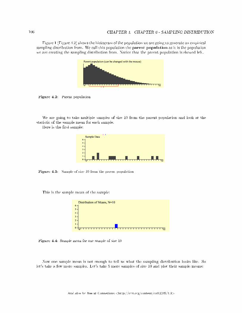
106 CHAPTER 4. CHAPTER 6 - SAMPLING DISTRIBUTION
Figure 1 (Figure 4.2) shows the histogram of the population we are going to generate an empiricalsampling distribution from. We call this population the parent population as it is the populationwe are creating the sampling distribution from. Notice that the parent population is skewed left.
Figure 4.2: Parent population
We are going to take multiple samples of size 10 from the parent population and look at thestatistic of the sample mean for each sample.
Here is the �rst sample:
Figure 4.3: Sample of size 10 from the parent population
This is the sample mean of the sample:
Figure 4.4: Sample mean for one sample of size 10
Now one sample mean is not enough to tell us what the sampling distribution looks like. Solet's take a few more samples. Let's take 5 more samples of size 10 and plot their sample means:
Available for free at Connexions <http://cnx.org/content/col12245/1.3>
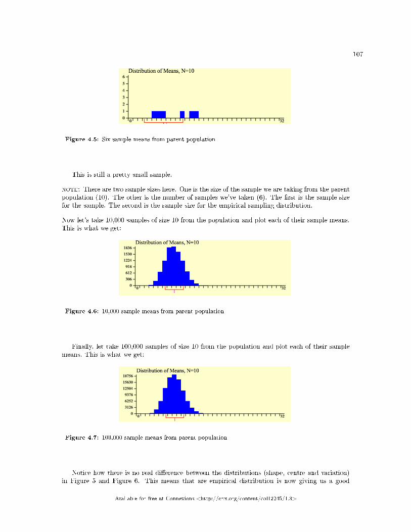
107
Figure 4.5: Six sample means from parent population
This is still a pretty small sample.
note: There are two sample sizes here. One is the size of the sample we are taking from the parentpopulation (10). The other is the number of samples we've taken (6). The �rst is the sample sizefor the sample. The second is the sample size for the empirical sampling distribution.
Now let's take 10,000 samples of size 10 from the population and plot each of their sample means.This is what we get:
Figure 4.6: 10,000 sample means from parent population
Finally, let take 100,000 samples of size 10 from the population and plot each of their samplemeans. This is what we get:
Figure 4.7: 100,000 sample means from parent population
Notice how there is no real di�erence between the distributions (shape, centre and variation)in Figure 5 and Figure 6. This means that are empirical distribution is now giving us a good
Available for free at Connexions <http://cnx.org/content/col12245/1.3>
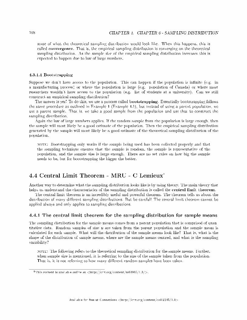
108 CHAPTER 4. CHAPTER 6 - SAMPLING DISTRIBUTION
sense of what the theoretical sampling distribution would look like. When this happens, this iscalled convergence. That is, the empirical sampling distribution is converging on the theoreticalsampling distribution. As the sample size of the empirical sampling distribution increases this isexpected to happen due to law of large numbers.
4.3.1.1 Bootstrapping
Suppose we don't have access to the population. This can happen if the population is in�nite (e.g. ina manufacturing process) or where the population is large (e.g. population of Canada) or where mostresearchers wouldn't have access to the population (e.g. list of students at a university). Can we stillconstruct an empirical sampling distribution?
The answer is yes! To do this, we use a process called bootstrapping. Essentially bootstrapping followsthe same procedure as outlined in Example 1 (Example 4.1), but instead of using a parent population, weuse a parent sample. That is, we take a good sample from the population and use that to construct thesampling distribution.
Again the law of large numbers applies. If the random sample from the population is large enough, thenthe sample will most likely be a good estimate of the population. Then the empirical sampling distributiongenerated by the sample will most likely be a good estimate of the theoretical sampling distribution of thepopulation.
note: Bootstrapping only works if the sample being used has been collected properly and thatthe sampling technique ensures that the sample is random, the sample is representative of thepopulation, and the sample size is large enough. There are no set rules on how big the sampleneeds to be, but for bootstrapping the bigger the better.
4.4 Central Limit Theorem - MRU - C Lemieux8
Another way to determine what the sampling distribution looks like is by using theory. The main theory thathelps us understand the characteristics of the sampling distribution is called the central limit theorem.
The central limit theorem is an incredibly useful and powerful theorem. The theorem tells us about thedistribution of many di�erent sampling distributions. But be careful! The central limit theorem cannot beapplied always and only applies to sampling distributions.
4.4.1 The central limit theorem for the sampling distribution for sample means
The sampling distribution for the sample means comes from a parent population that is comprised of quan-titative data. Random samples of size n are taken from the parent population and the sample mean iscalculated for each sample. What will the distribution of the sample means look like? That is, what is theshape of the distribution of sample means, where are the sample means centred, and what is the samplingvariability?
note: The following refers to the theoretical sampling distribution for the sample means. Further,when sample size is mentioned, it is referring to the size of the sample taken from the population.That is, it is not referring to how many di�erent random samples have been taken.
8This content is available online at <http://cnx.org/content/m64935/1.3/>.
Available for free at Connexions <http://cnx.org/content/col12245/1.3>
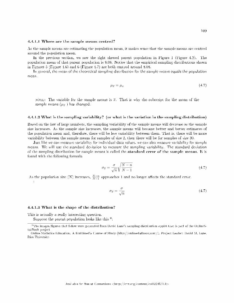
109
4.4.1.1 Where are the sample means centred?
As the sample means are estimating the population mean, it makes sense that the sample means are centredaround the population mean.
In the previous section, we saw the right skewed parent population in Figure 1 (Figure 4.2). Thepopulation mean of that parent population is 8.08. Notice that the empirical sampling distributions shownin Figures 5 (Figure 4.6) and 6 (Figure 4.7) are both centred around 8.08.
In general, the mean of the theoretical sampling distribution for the sample means equals the populationmean.
µx = µx (4.7)
note: The variable for the sample means is x. That is why the subscript for the mean of thesample means (µx ) has changed.
4.4.1.2 What is the sampling variability? (or what is the variation in the sampling distribution)
Based on the law of large numbers, the sampling variability of the sample means will decrease as the samplesize increases. As the sample size increases, the sample means will become better and better estimates ofthe population mean and, therefore, there will be less variability between them. That is, there will be morevariability between the sample means for samples of size 2, then there will be for samples of size 30.
Just like we can measure variability for individual data values, we can also measure variability for samplemeans. We will use the standard deviation to measure the sampling variability. The standard deviationof the sampling distribution for sample means is called the standard error of the sample means. It isfound with the following formula
σx =σ√n
√N − nN − 1
(4.7)
As the population size (N) increases, N−nN−1 approaches 1 and no longer a�ects the standard error.:
σx =σ√n
(4.7)
4.4.1.3 What is the shape of the distribution?
This is actually a really interesting question.Suppose the parent population looks like this 9:
9The images/�gures that follow were generated from David Lane's sampling distribution applet that is part of the OnlineS-tatBook projectOnline Statistics Education: A Multimedia Course of Study (http://onlinestatbook.com/). Project Leader: David M. Lane,
Rice University.
Available for free at Connexions <http://cnx.org/content/col12245/1.3>
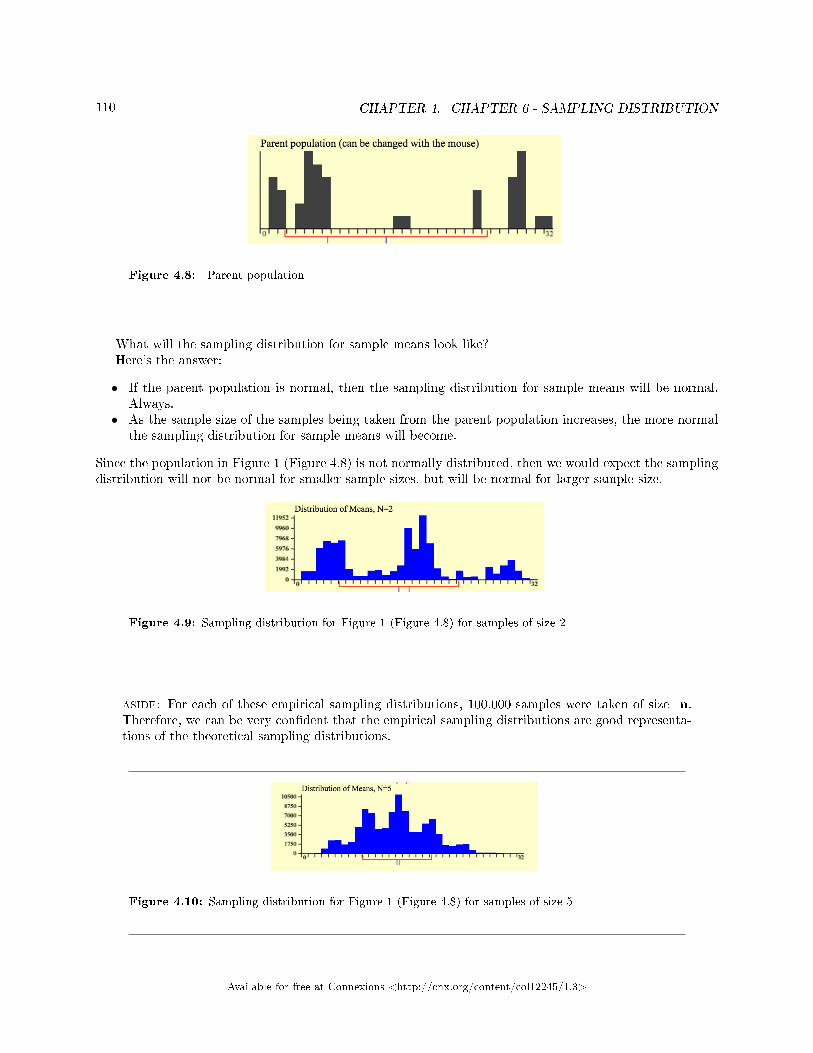
110 CHAPTER 4. CHAPTER 6 - SAMPLING DISTRIBUTION
Figure 4.8: Parent population
What will the sampling distribution for sample means look like?Here's the answer:
• If the parent population is normal, then the sampling distribution for sample means will be normal.Always.
• As the sample size of the samples being taken from the parent population increases, the more normalthe sampling distribution for sample means will become.
Since the population in Figure 1 (Figure 4.8) is not normally distributed, then we would expect the samplingdistribution will not be normal for smaller sample sizes, but will be normal for larger sample size.
Figure 4.9: Sampling distribution for Figure 1 (Figure 4.8) for samples of size 2
aside: For each of these empirical sampling distributions, 100,000 samples were taken of size n.Therefore, we can be very con�dent that the empirical sampling distributions are good representa-tions of the theoretical sampling distributions.
Figure 4.10: Sampling distribution for Figure 1 (Figure 4.8) for samples of size 5
Available for free at Connexions <http://cnx.org/content/col12245/1.3>
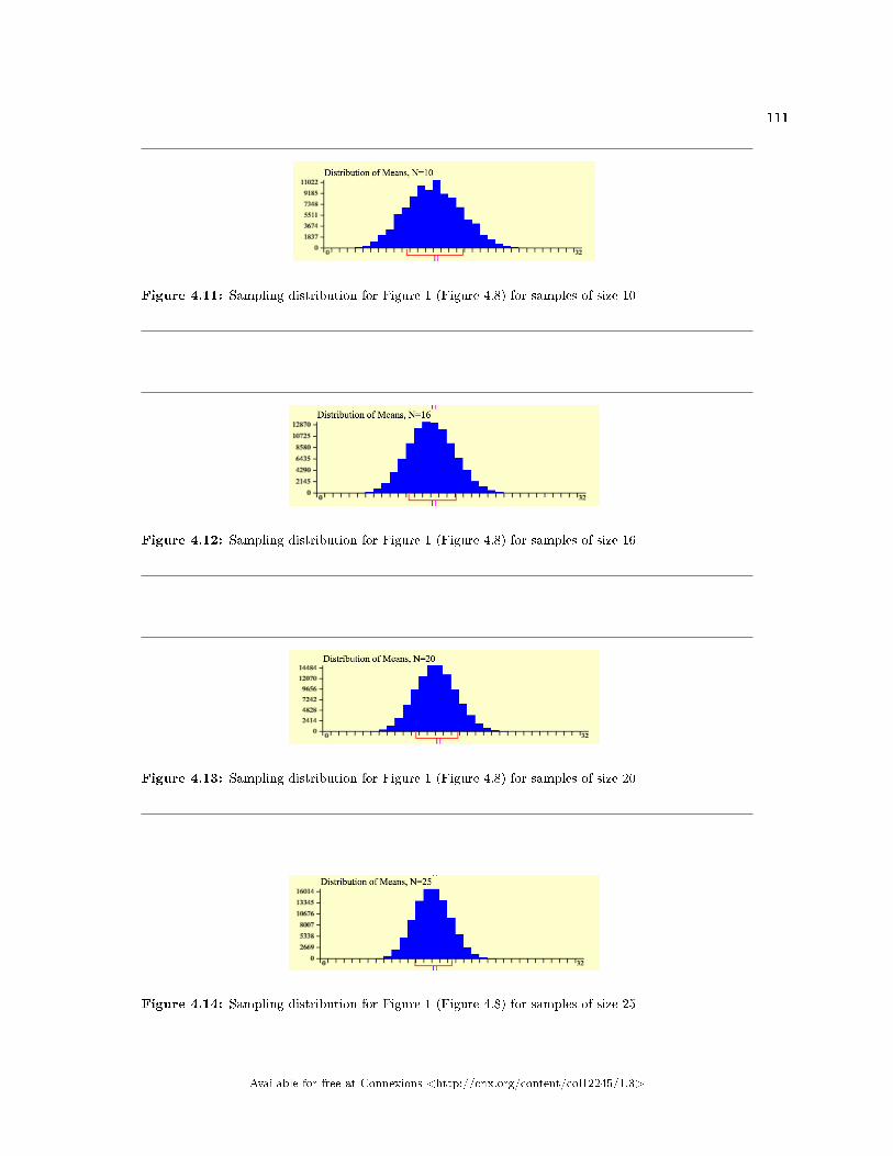
111
Figure 4.11: Sampling distribution for Figure 1 (Figure 4.8) for samples of size 10
Figure 4.12: Sampling distribution for Figure 1 (Figure 4.8) for samples of size 16
Figure 4.13: Sampling distribution for Figure 1 (Figure 4.8) for samples of size 20
Figure 4.14: Sampling distribution for Figure 1 (Figure 4.8) for samples of size 25
Available for free at Connexions <http://cnx.org/content/col12245/1.3>
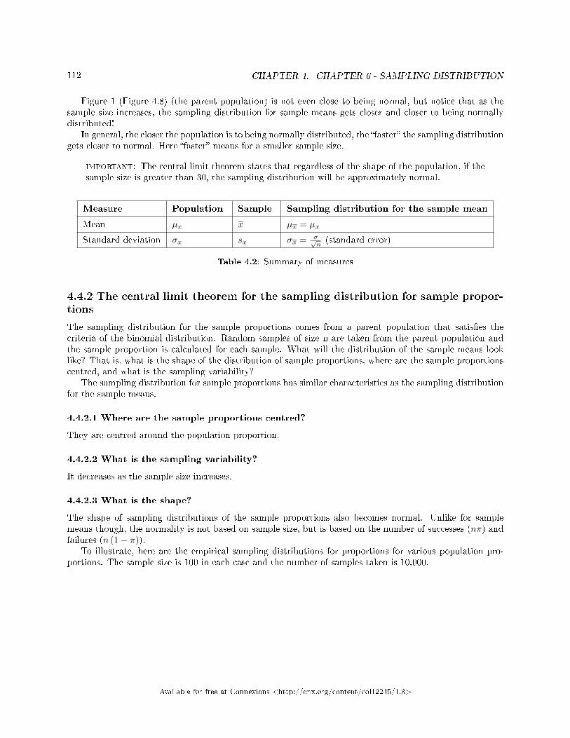
112 CHAPTER 4. CHAPTER 6 - SAMPLING DISTRIBUTION
Figure 1 (Figure 4.8) (the parent population) is not even close to being normal, but notice that as thesample size increases, the sampling distribution for sample means gets closer and closer to being normallydistributed!
In general, the closer the population is to being normally distributed, the �faster� the sampling distributiongets closer to normal. Here �faster� means for a smaller sample size.
important: The central limit theorem states that regardless of the shape of the population, if thesample size is greater than 30, the sampling distribution will be approximately normal.
Measure Population Sample Sampling distribution for the sample mean
Mean µx x µx = µx
Standard deviation σx sx σx = σ√n(standard error)
Table 4.2: Summary of measures
4.4.2 The central limit theorem for the sampling distribution for sample propor-
tions
The sampling distribution for the sample proportions comes from a parent population that satis�es thecriteria of the binomial distribution. Random samples of size n are taken from the parent population andthe sample proportion is calculated for each sample. What will the distribution of the sample means looklike? That is, what is the shape of the distribution of sample proportions, where are the sample proportionscentred, and what is the sampling variability?
The sampling distribution for sample proportions has similar characteristics as the sampling distributionfor the sample means.
4.4.2.1 Where are the sample proportions centred?
They are centred around the population proportion.
4.4.2.2 What is the sampling variability?
It decreases as the sample size increases.
4.4.2.3 What is the shape?
The shape of sampling distributions of the sample proportions also becomes normal. Unlike for samplemeans though, the normality is not based on sample size, but is based on the number of successes (nπ) andfailures (n (1− π)).
To illustrate, here are the empirical sampling distributions for proportions for various population pro-portions. The sample size is 100 in each case and the number of samples taken is 10,000.
Available for free at Connexions <http://cnx.org/content/col12245/1.3>
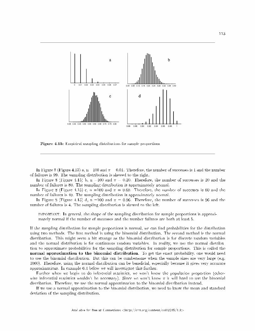
113
Figure 4.15: Empirical sampling distributions for sample proportions
In Figure 8 (Figure 4.15) a, n =100 and π = 0.01. Therefore, the number of successes is 1 and the numberof failures is 99. The sampling distribution is skewed to the right.
In Figure 8 (Figure 4.15) b, n =100 and π = 0.20. Therefore, the number of successes is 20 and thenumber of failures is 80. The sampling distribution is approximately normal.
In Figure 8 (Figure 4.15) c, n =100 and π = 0.60. Therefore, the number of successes is 60 and thenumber of failures is 40. The sampling distribution is approximately normal.
In Figure 8 (Figure 4.15) d, n =100 and π = 0.96. Therefore, the number of successes is 96 and thenumber of failures is 4. The sampling distribution is skewed to the left.
important: In general, the shape of the sampling distribution for sample proportions is approxi-mately normal if the number of successes and the number failures are both at least 5.
If the sampling distribution for sample proportions is normal, we can �nd probabilities for the distributionusing two methods. The �rst method is using the binomial distribution. The second method is the normaldistribution. This might seem a bit strange as the binomial distribution is for discrete random variablesand the normal distribution is for continuous random variables. In reality, we use the normal distribu-tion to approximate probabilities for the sampling distribution for sample proportions. This is called thenormal approximation to the binomial distribution. To get the exact probability, one would needto use the binomial distribution. But this can be cumbersome when the sample sizes are very large (e.g.1000). Therefore, using the normal distribution can be bene�cial, especially because it gives very accurateapproximations. In example 6.4 below we will investigate this further.
Further when we begin to do inferential statistics, we won't know the population proportion (other-wise inferential statistics wouldn't be necessary). Since we won't know π it will hard to use the binomialdistribution. Therefore, we use the normal approximation to the binomial distribution instead.
If we use a normal approximation to the binomial distribution, we need to know the mean and standarddeviation of the sampling distribution.
Available for free at Connexions <http://cnx.org/content/col12245/1.3>
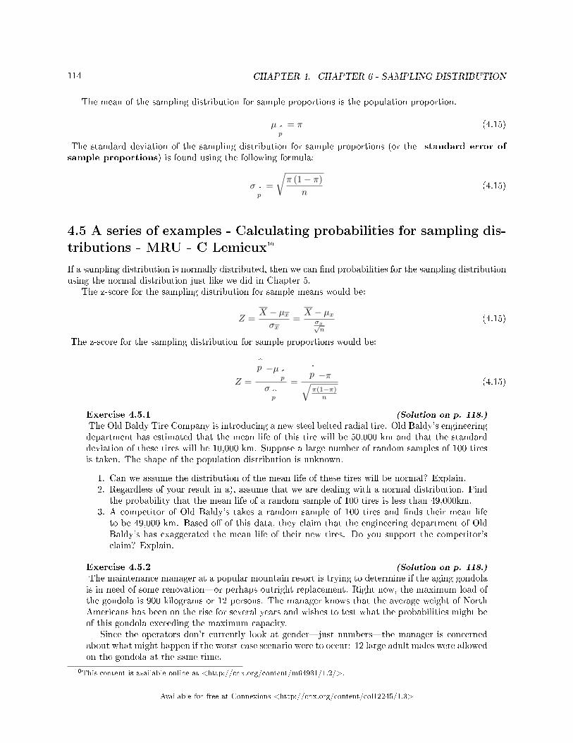
114 CHAPTER 4. CHAPTER 6 - SAMPLING DISTRIBUTION
The mean of the sampling distribution for sample proportions is the population proportion.
µp̂
= π (4.15)
The standard deviation of the sampling distribution for sample proportions (or the standard error ofsample proportions) is found using the following formula:
σp̂
=
√π (1− π)
n(4.15)
4.5 A series of examples - Calculating probabilities for sampling dis-tributions - MRU - C Lemieux10
If a sampling distribution is normally distributed, then we can �nd probabilities for the sampling distributionusing the normal distribution just like we did in Chapter 5.
The z-score for the sampling distribution for sample means would be:
Z =X − µxσx
=X − µx
σx√n
(4.15)
The z-score for the sampling distribution for sample proportions would be:
Z =
^p −µ
p̂
σp̂
=
^p −π√π(1−π)
n
(4.15)
Exercise 4.5.1 (Solution on p. 118.)
The Old Baldy Tire Company is introducing a new steel belted radial tire. Old Baldy's engineeringdepartment has estimated that the mean life of this tire will be 50,000 km and that the standarddeviation of these tires will be 10,000 km. Suppose a large number of random samples of 100 tiresis taken. The shape of the population distribution is unknown.
1. Can we assume the distribution of the mean life of these tires will be normal? Explain.2. Regardless of your result in a), assume that we are dealing with a normal distribution. Find
the probability that the mean life of a random sample of 100 tires is less than 49,000km.3. A competitor of Old Baldy's takes a random sample of 100 tires and �nds their mean life
to be 49,000 km. Based o� of this data, they claim that the engineering department of OldBaldy's has exaggerated the mean life of their new tires. Do you support the competitor'sclaim? Explain.
Exercise 4.5.2 (Solution on p. 118.)
The maintenance manager at a popular mountain resort is trying to determine if the aging gondolais in need of some renovation�or perhaps outright replacement. Right now, the maximum load ofthe gondola is 900 kilograms or 12 persons. The manager knows that the average weight of NorthAmericans has been on the rise for several years and wishes to test what the probabilities might beof this gondola exceeding the maximum capacity.
Since the operators don't currently look at gender�just numbers�the manager is concernedabout what might happen if the worst-case scenario were to occur: 12 large adult males were allowedon the gondola at the same time.
10This content is available online at <http://cnx.org/content/m64931/1.2/>.
Available for free at Connexions <http://cnx.org/content/col12245/1.3>
115
To investigate this further the manager did some research into the current average weight ofadult males and discovered that it is about 80 kilograms. He also knows that adult weight tendsto be normally distributed by gender, with a standard deviation for males of about 12 kilograms.
a. Given this information, he �rst wants to know what the individual weight allowance is (i.e.the per person average) that the gondola can withstand.
b. He also wants to know how likely is it that the individual weight of any randomly selectedmale will exceed the individual weight allowance calculated above.
c. Finally, he wants to know how likely it would be that the average weight of a sample of 12adult males would exceed the average individual weight allowance.
d. Based on your answers, do you think the manager should renovate the gondola? Is there anyfurther information that the manager would need?
Exercise 4.5.3 (Solution on p. 118.)
The city of Montreal has an extensive bike lane system. In fact, it is one of the largest in NorthAmerica. But many cyclists �nd that even with all of the bike lanes, it is still hard to get around thecity on a bike. In particular, there are many lanes that run east/west, but few that run north/south.Thus, they are encouraging the city council to focus less on adding lots of kilometers to the system,but instead making sure that the current system properly connects all parts of the city.
The city council will only go forward with this idea if at least 66% of the residents supportfocusing on connecting the system rather than expanding the system.
Suppose that 62% of residents do support connecting the system rather than expanding it.What is the probability that a random sample of 1000 residents will have a sample proportion ofat least 66%?
a. Find the above probability using the binomial distribution.b. Find the above probability by using the sampling distribution for sample proportions.c. Compare the two answers. Do they give similar answers?d. Based on your answers, do you think that it is possible that the city of Montreal will choose
to focus on connecting the bike path system?
Exercise 4.5.4 (Solution on p. 119.)
Video games are gaining more and more popularity. Children often try to convince their parentsto buy games even when they are not appropriate. For example, they may want to play a veryviolent game that is not appropriate for their age group. To help parents out, video games haverating categories to suggest age appropriateness. But how aware are parents of these categories?
To investigate this, you conduct a survey of Canadian families that have young children whoplay video games. You show parents three video game covers that have the category rating clearlymarked on it. You then ask the parents whether the games would be appropriate for children andwhy. If the parent correctly identi�es which games are appropriate for their children and refers tothe ratings in making their choice, you categorize the parents as well informed.
Suppose that we want to use your results to justify the claim that less than 30 percent of parentsare well informed about video game ratings. In your random sample of 1000 parents, you actuallyfound that 27 percent of the parents that you polled were well informed about video game ratings.
a. Assuming that the proportion of parents that are well informed about video game ratings is30%, what is the probability that you would observe a sample proportion of less than 27%.Use the normal approximation of the binomial distribution to �nd your answer.
b. Based on your results, do you believe that this is enough evidence to suggest that less than30% of parents are well informed about video game ratings? Explain your answer.
Available for free at Connexions <http://cnx.org/content/col12245/1.3>
116 CHAPTER 4. CHAPTER 6 - SAMPLING DISTRIBUTION
4.5.1 Practice questions
The following practice questions are from Lyryx Learning, Business Statistics I � MGMT 2262 � Mt RoyalUniversity � Version 2016 Revision A. OpenStax CNX. Sep 8, 2016 http://cnx.org/contents/[email protected]
Use the following information to answer the next ten exercises: A manufacturer produces 25-pound liftingweights. The lowest actual weight is 24 pounds, and the highest is 26 pounds. Each weight is equally likelyso the distribution of weights is uniform. A sample of 100 weights is taken. The standard deviation is 0.58pounds.
Exercise 4.5.5 (Solution on p. 119.)
a. What is the distribution for the weights of one 25-pound lifting weight? What is the meanand standard deivation?
b. What is the distribution for the mean weight of 100 25-pound lifting weights?c. Find the probability that the mean actual weight for the 100 weights is less than 24.9.
Exercise 4.5.6 (Solution on p. 119.)
Find the probability that the mean actual weight for the 100 weights is greater than 25.2.
Exercise 4.5.7 (Solution on p. 119.)
Find the 90th percentile for the mean weight for the 100 weights.
Exercise 4.5.8 (Solution on p. 119.)
Suppose that the distance of �y balls hit to the out�eld (in baseball) is normally distributed witha mean of 250 feet and a standard deviation of 50 feet. We randomly sample 49 �y balls.
a. What is the probability that the 49 balls traveled an average of less than 240 feet?b. Find the 80th percentile of the distribution of the average of 49 �y balls.
Exercise 4.5.9 (Solution on p. 119.)
According to the Internal Revenue Service, the average length of time for an individual to complete(keep records for, learn, prepare, copy, assemble, and send) IRS Form 1040 is 10.53 hours (withoutany attached schedules). The distribution is unknown. Let us assume that the standard deviationis two hours. Suppose we randomly sample 36 taxpayers.
a. Would you be surprised if the 36 taxpayers �nished their Form 1040s in an average of morethan 12 hours? Explain why or why not in complete sentences.
b. Would you be surprised if one taxpayer �nished his or her Form 1040 in more than 12 hours?In a complete sentence, explain why.
Exercise 4.5.10 (Solution on p. 119.)
Suppose that a category of world-class runners are known to run a marathon (26 miles) in an
average of 145 minutes with a standard deviation of 14 minutes. Consider 49 of the races. Let−−X
the average of the 49 races.
a. Find the probability that the runner will average between 142 and 146 minutes in these 49marathons.
b. Find the 80th percentile for the average of these 49 marathons.c. Find the median of the average running times.
Exercise 4.5.11 (Solution on p. 119.)
Determine which of the following are true and which are false. Then, in complete sentences, justifyyour answers.
Available for free at Connexions <http://cnx.org/content/col12245/1.3>
117
a. When the sample size is large, the mean of−−X is approximately equal to the mean of X.
b. When the sample size is large,−−X is approximately normally distributed.
c. When the sample size is large, the standard deviation of−−X is approximately the same as the
standard deviation of X.
Available for free at Connexions <http://cnx.org/content/col12245/1.3>
118 CHAPTER 4. CHAPTER 6 - SAMPLING DISTRIBUTION
Solutions to Exercises in Chapter 4
Solution to Exercise 4.5.1 (p. 114)
a. Yes. As the sample size is greater than 30 (it is 100), we can assume that the sampling distribution ofthe sample mean lifespan of the tires is normally distributed regardless of the shape of the samplingdistribution due to the central limit theorem.
b. x = mean lifespan of 100 Old Baldy tires, µx = µx = 50,000, σx = σ√n= 10,000/10 = 1000. Since we
know that the data is normally distributed, we can use a computer program to calculate the probabilityP(X < 49, 000
). From the computer program, we get P
(X < 49, 000
)= 15.87%
c. No. The probability that a random sample of 100 Old Baldy tires has a mean lifespan of 49,000km is15.87% (assuming Old Baldy's claim). This means that this event is likely to occur (as it is greater than10%), under the assumption that the tires last on average 50,000 km, and does not provide su�cientevidence against Old Baldy's claim.
Solution to Exercise 4.5.2 (p. 114)
a. 900kg/12 people = 75kg/personb. Since this is about an individual, we will use µx and σx. As stated in the question, we know that
the population is normally distributed. From this, a computer program calculated that P (X ≥ 75) =66.15%, where X is the weight of an individual person on the gondola.
c. Now, we are being asked about the mean for 12 people. Therefore, this question is about �nding aprobability for the sampling distribution for sample means. Therefore, we will use x = mean weightof 12 people, µx = µx = 80, σx = σ√
n= 12/3.46 = 3.46. Since the population distribution is normal,
we know that the sampling distribution will also be normal (regardless of the sample size). Therefore,we can use a computer program to calculate the probability P
(X > 75
). We get 92.55%.
d. The probability found in c) is the probability that the average mass of 12 adult males will exceed themaximum individual weight for the gondola. The next question is �how likely is it that there will be12 adult males on the gondola?� The manager should do further research to determine this beforemaking a decision. While waiting for the results, the manager should implement a policy where anylarge groups of males are broken up and are required to take the lift in separate groups. I.e. break upa group of 12 males into two groups of 6 males.
Solution to Exercise 4.5.3 (p. 115)
a. Since we are using the binomial distribution, we are being asked to �nd the probability that at least660 of the 1000 people in the poll will want to focus on connecting the system. The 660 comes from66% of 1000. In other words, we are asked to �nd the P (X ≥ 660) , with n = 1000 and π = 60%. Usinga computer program, this yields a probability of 0.48%. This is found, by highlighting all of the valuesabove 660 and including 660.
b. Since we are using the sampling distribution for sample proportions, we are asked to �nd the probability
that the sample proportion will be at least 66%. In other words, we are asked to �nd the P(^p≥ 0.66).
We can assume the sampling distribution for sample proportions is normal as the number of successes(nπ =1000 × 0.62=620) and the number of failures (n (1− π) = 1000 × 0.38=380) are both at least�ve. Therefore, we will use the normal distribution to �nd the probability with µ
p̂
= π = 0.62 and
σp̂
=√
π(1−π)n =
√0.62(1−0.62)
1000 = 0.01475. Therefore, using a computer program we �nd P(^p≥ 0.66)
= 0.33%c. The two probabilities are quite close. They are only 0.15% apart. Therefore, the two methods give us
similar results.d. It is unlikely that if the proportion of residents that want to focus on connecting the bike system is
62% that a poll of 1000 people would result in a sample proportion of 66%. Therefore, it is unlikelythat the city of Montreal will chose to focus on connecting the system.
Available for free at Connexions <http://cnx.org/content/col12245/1.3>

119
Solution to Exercise 4.5.4 (p. 115)
a. Since we are using the sampling distribution for sample proportions, we are asked to �nd the probability
that the sample proportion will be at most 27%. In other words, we are asked to �nd the P(^p≤
0.27). We can assume the sampling distribution for sample proportions is normal as the number ofsuccesses ( and the number of failures ((nπ =1000 × 0.30=300) and the number of failures (n (1− π)= 1000 × 0.7=700) are both at least �ve. Therefore, we will use the normal distribution to �nd the
probability with µp̂
= π = 0.30 and σp̂
=√
π(1−π)n =
√0.3(1−0.3)
1000 = 0.01145. Therefore, using a
computer program we �nd P(^p≤ 0.27) = 0.44%.
b. Since the probability that we would observe a sample proportion of 27% (assuming a populationproportion of 30%) is 0.44%, it is very unlikely we would have observed this evidence if the assumptionis true. Therefore, it is more likely that the population proportion is less than 30%. Thus there isenough evidence to suggest that less than 30% of parents are well informed about video game ratings.
Solution to Exercise 4.5.5 (p. 116)
a. Uniform with a mean of 25 and a standard deviation of 0.58 pounds. Remember when a distributionis uniform all of the values are equally likely. Therefore the mean will be halfway between the lowestvalue (24) and the highest value (26).
b. Normal with a mean of 25 and a standard deviation of 0.0577c. 0.0416
Solution to Exercise 4.5.6 (p. 116)0.0003Solution to Exercise 4.5.7 (p. 116)25.07Solution to Exercise 4.5.8 (p. 116)
a. 0.0808b. 256.01 feet
Solution to Exercise 4.5.9 (p. 116)
a. Yes. I would be surprised, because the probability is almost 0.b. No. I would not be totally surprised because the probability is 0.2312
Solution to Exercise 4.5.10 (p. 116)
a. 0.6247b. 146.68c. 145 minutes
Solution to Exercise 4.5.11 (p. 116)
a. True. The mean of a sampling distribution of the means is approximately the mean of the datadistribution.
b. True. According to the Central Limit Theorem, the larger the sample, the closer the sampling distri-bution of the means becomes normal.
c. The standard deviation of the sampling distribution of the means will decrease making it approximatelythe same as the standard deviation of X as the sample size increases.
Available for free at Connexions <http://cnx.org/content/col12245/1.3>
120 GLOSSARY
Glossary
C Conditional Probability
the likelihood that an event will occur given that another event has already occurred
Contingency Table
the method of displaying a frequency distribution as a table with rows and columns to show howtwo variables may be dependent (contingent) upon each other; the table provides an easy way tocalculate conditional probabilities.
D Dependent Events
If two events are NOT independent, then we say that they are dependent.
E Equally Likely
Each outcome of an experiment has the same probability.
Event
a subset of the set of all outcomes of an experiment; the set of all outcomes of an experiment iscalled a sample space and is usually denoted by S. An event is an arbitrary subset in S. It cancontain one outcome, two outcomes, no outcomes (empty subset), the entire sample space, andthe like. Standard notations for events are capital letters such as A, B, C, and so on.
Experiment
a planned activity carried out under controlled conditions
I Independent Events
The occurrence of one event has no e�ect on the probability of the occurrence of another event.Events A and B are independent if one of the following is true:
• P(A|B) = P(A)• P(B|A) = P(B)• P(A ∩ B) = P(A)P(B)
M Mutually Exclusive
Two events are mutually exclusive if the probability that they both happen at the same time iszero. If events A and B are mutually exclusive, then P(A ∩ B) = 0.
N Normal Distribution
a continuous random variable (RV) with pdf f (x) =
1
σ√2π
e−−(x −− µ)
2σ2
2
, where µ is the mean of the distribution and σ is the standard deviation; notation: X ∼ N(µ,σ). If µ = 0 and σ = 1, the RV, Z, is called the standard normal distribution.
O Outcome
Available for free at Connexions <http://cnx.org/content/col12245/1.3>
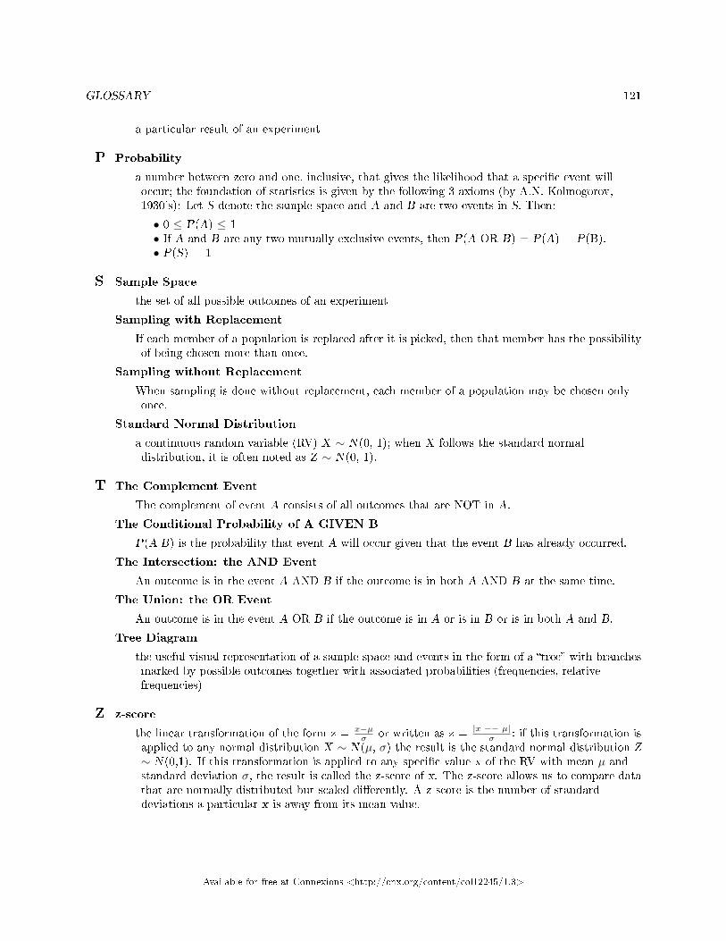
GLOSSARY 121
a particular result of an experiment
P Probability
a number between zero and one, inclusive, that gives the likelihood that a speci�c event willoccur; the foundation of statistics is given by the following 3 axioms (by A.N. Kolmogorov,1930's): Let S denote the sample space and A and B are two events in S. Then:
• 0 ≤ P(A) ≤ 1• If A and B are any two mutually exclusive events, then P(A OR B) = P(A) + P(B).• P(S) = 1
S Sample Space
the set of all possible outcomes of an experiment
Sampling with Replacement
If each member of a population is replaced after it is picked, then that member has the possibilityof being chosen more than once.
Sampling without Replacement
When sampling is done without replacement, each member of a population may be chosen onlyonce.
Standard Normal Distribution
a continuous random variable (RV) X ∼ N(0, 1); when X follows the standard normaldistribution, it is often noted as Z ∼ N(0, 1).
T The Complement Event
The complement of event A consists of all outcomes that are NOT in A.
The Conditional Probability of A GIVEN B
P(A|B) is the probability that event A will occur given that the event B has already occurred.
The Intersection: the AND Event
An outcome is in the event A AND B if the outcome is in both A AND B at the same time.
The Union: the OR Event
An outcome is in the event A OR B if the outcome is in A or is in B or is in both A and B.
Tree Diagram
the useful visual representation of a sample space and events in the form of a �tree� with branchesmarked by possible outcomes together with associated probabilities (frequencies, relativefrequencies)
Z z-score
the linear transformation of the form z = x−µσ or written as z = |x −− µ|
σ ; if this transformation isapplied to any normal distribution X ∼ N(µ, σ) the result is the standard normal distribution Z∼ N(0,1). If this transformation is applied to any speci�c value x of the RV with mean µ andstandard deviation σ, the result is called the z-score of x. The z-score allows us to compare datathat are normally distributed but scaled di�erently. A z-score is the number of standarddeviations a particular x is away from its mean value.
Available for free at Connexions <http://cnx.org/content/col12245/1.3>
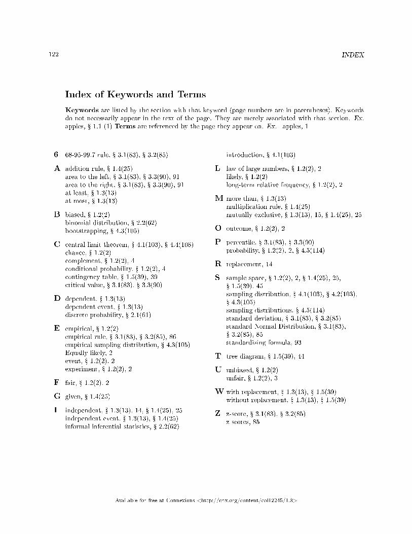
122 INDEX
Index of Keywords and Terms
Keywords are listed by the section with that keyword (page numbers are in parentheses). Keywordsdo not necessarily appear in the text of the page. They are merely associated with that section. Ex.apples, � 1.1 (1) Terms are referenced by the page they appear on. Ex. apples, 1
6 68-95-99.7 rule, � 3.1(83), � 3.2(85)
A addition rule, � 1.4(25)area to the left, � 3.1(83), � 3.3(90), 91area to the right, � 3.1(83), � 3.3(90), 91at least, � 1.3(13)at most, � 1.3(13)
B biased, � 1.2(2)binomial distribution, � 2.2(62)bootstrapping, � 4.3(105)
C central limit theorem, � 4.1(103), � 4.4(108)chance, � 1.2(2)complement, � 1.2(2), 4conditional probability, � 1.2(2), 4contingency table, � 1.5(39), 39critical value, � 3.1(83), � 3.3(90)
D dependent, � 1.3(13)dependent event, � 1.3(13)discrete probability, � 2.1(61)
E empirical, � 1.2(2)empirical rule, � 3.1(83), � 3.2(85), 86empirical sampling distribution, � 4.3(105)Equally likely, 2event, � 1.2(2), 2experiment, � 1.2(2), 2
F fair, � 1.2(2), 2
G given, � 1.4(25)
I independent, � 1.3(13), 14, � 1.4(25), 25independent event, � 1.3(13), � 1.4(25)informal inferential statistics, � 2.2(62)
introduction, � 4.1(103)
L law of large numbers, � 1.2(2), 2likely, � 1.2(2)long-term relative frequency, � 1.2(2), 2
M more than, � 1.3(13)multiplication rule, � 1.4(25)mutually exclusive, � 1.3(13), 15, � 1.4(25), 25
O outcome, � 1.2(2), 2
P percentile, � 3.1(83), � 3.3(90)probability, � 1.2(2), 2, � 4.5(114)
R replacement, 14
S sample space, � 1.2(2), 2, � 1.4(25), 25,� 1.5(39), 45sampling distribution, � 4.1(103), � 4.2(103),� 4.3(105)sampling distributions, � 4.5(114)standard deviation, � 3.1(83), � 3.2(85)standard Normal Distribution, � 3.1(83),� 3.2(85), 85standardizing formula, 93
T tree diagram, � 1.5(39), 44
U unbiased, � 1.2(2)unfair, � 1.2(2), 3
W with replacement, � 1.3(13), � 1.5(39)without replacement, � 1.3(13), � 1.5(39)
Z z-score, � 3.1(83), � 3.2(85)z-scores, 85
Available for free at Connexions <http://cnx.org/content/col12245/1.3>

ATTRIBUTIONS 123
Attributions
Collection: Business Statistics - Unit 2 - ProbabilityEdited by: Collette LemieuxURL: http://cnx.org/content/col12245/1.3/License: http://creativecommons.org/licenses/by/4.0/
Module: "Introduction � Probability Topics � MtRoyal - Version2016RevA"By: Lyryx LearningURL: http://cnx.org/content/m62328/1.1/Pages: 1-2Copyright: Lyryx LearningLicense: http://creativecommons.org/licenses/by/4.0/Based on: IntroductionBy: OpenStax, OpenStax Business StatisticsURL: http://cnx.org/content/m54216/1.1/
Module: "Terminology � Probability Topics � MtRoyal - Version2016RevA"By: Lyryx LearningURL: http://cnx.org/content/m62337/1.3/Pages: 2-13Copyright: Lyryx LearningLicense: http://creativecommons.org/licenses/by/4.0/Based on: TerminologyBy: OpenStax, OpenStax Business StatisticsURL: http://cnx.org/content/m54218/1.8/
Module: "Independent and Mutually Exclusive Events � Probaility Topics � MtRoyal - Version2016RevA"By: Lyryx LearningURL: http://cnx.org/content/m62329/1.2/Pages: 13-25Copyright: Lyryx LearningLicense: http://creativecommons.org/licenses/by/4.0/Based on: Independent and Mutually Exclusive EventsBy: OpenStax, OpenStax Business StatisticsURL: http://cnx.org/content/m54219/1.2/
Module: "Two Basic Rules of Probability"By: OpenStaxURL: http://cnx.org/content/m54220/1.14/Pages: 25-38Copyright: Rice UniversityLicense: http://creativecommons.org/licenses/by/4.0/Based on: Two Basic Rules of ProbabilityBy: OpenStaxURL: http://cnx.org/content/m46947/1.4/
Available for free at Connexions <http://cnx.org/content/col12245/1.3>
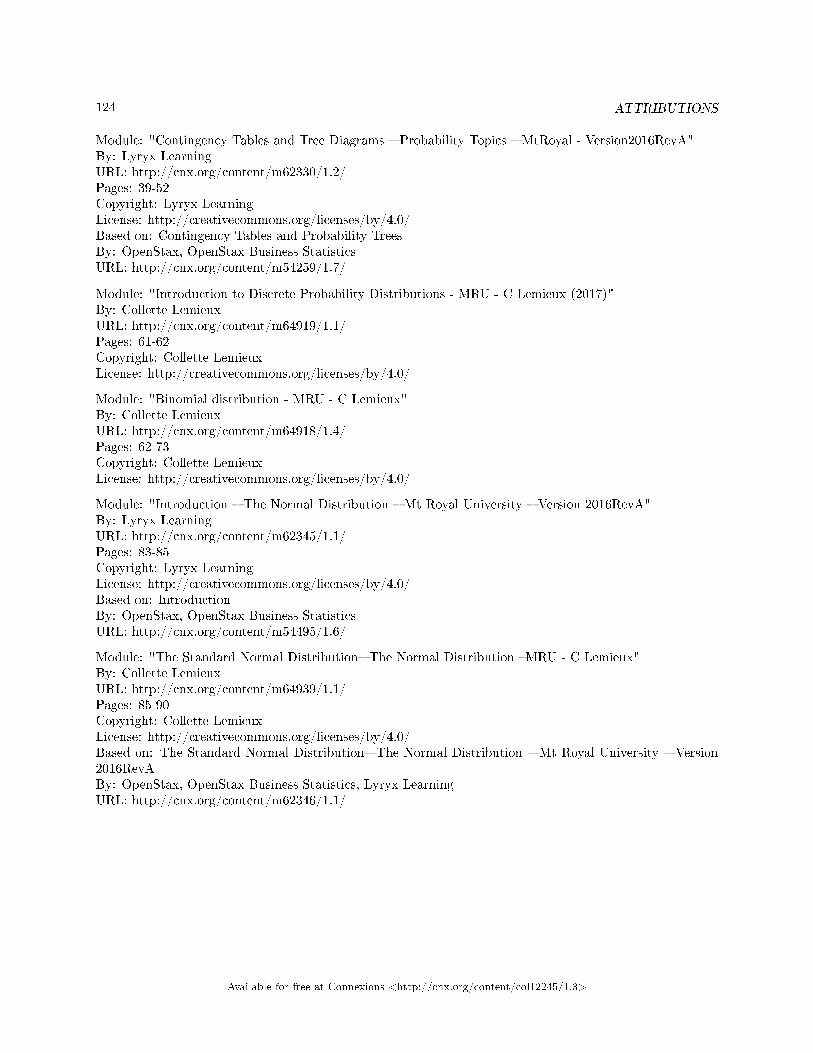
124 ATTRIBUTIONS
Module: "Contingency Tables and Tree Diagrams � Probability Topics � MtRoyal - Version2016RevA"By: Lyryx LearningURL: http://cnx.org/content/m62330/1.2/Pages: 39-52Copyright: Lyryx LearningLicense: http://creativecommons.org/licenses/by/4.0/Based on: Contingency Tables and Probability TreesBy: OpenStax, OpenStax Business StatisticsURL: http://cnx.org/content/m54259/1.7/
Module: "Introduction to Discrete Probability Distributions - MRU - C Lemieux (2017)"By: Collette LemieuxURL: http://cnx.org/content/m64919/1.1/Pages: 61-62Copyright: Collette LemieuxLicense: http://creativecommons.org/licenses/by/4.0/
Module: "Binomial distribution - MRU - C Lemieux"By: Collette LemieuxURL: http://cnx.org/content/m64918/1.4/Pages: 62-73Copyright: Collette LemieuxLicense: http://creativecommons.org/licenses/by/4.0/
Module: "Introduction � The Normal Distribution � Mt Royal University � Version 2016RevA"By: Lyryx LearningURL: http://cnx.org/content/m62345/1.1/Pages: 83-85Copyright: Lyryx LearningLicense: http://creativecommons.org/licenses/by/4.0/Based on: IntroductionBy: OpenStax, OpenStax Business StatisticsURL: http://cnx.org/content/m54495/1.6/
Module: "The Standard Normal Distribution� The Normal Distribution �MRU - C Lemieux"By: Collette LemieuxURL: http://cnx.org/content/m64939/1.1/Pages: 85-90Copyright: Collette LemieuxLicense: http://creativecommons.org/licenses/by/4.0/Based on: The Standard Normal Distribution� The Normal Distribution � Mt Royal University � Version2016RevABy: OpenStax, OpenStax Business Statistics, Lyryx LearningURL: http://cnx.org/content/m62346/1.1/
Available for free at Connexions <http://cnx.org/content/col12245/1.3>
ATTRIBUTIONS 125
Module: "Using the Normal Distribution� The Normal Distribution � MRU - C Lemieux"By: Collette LemieuxURL: http://cnx.org/content/m64940/1.2/Pages: 90-101Copyright: Collette LemieuxLicense: http://creativecommons.org/licenses/by/4.0/Based on: Using the Normal Distribution� The Normal Distribution � Mt Royal University � Version2016RevABy: OpenStax, OpenStax Business Statistics, Lyryx LearningURL: http://cnx.org/content/m62347/1.1/
Module: "Introduction - Sampling distributions - MRU - C Lemieux"By: Collette LemieuxURL: http://cnx.org/content/m64933/1.1/Page: 103Copyright: Collette LemieuxLicense: http://creativecommons.org/licenses/by/4.0/
Module: "Introduction to Sampling Distributions"By: Collette LemieuxURL: http://cnx.org/content/m64932/1.2/Pages: 103-105Copyright: Collette LemieuxLicense: http://creativecommons.org/licenses/by/4.0/
Module: "Constructing empirical sampling distributions - MRU - C Lemieux"By: Collette LemieuxURL: http://cnx.org/content/m64934/1.2/Pages: 105-108Copyright: Collette LemieuxLicense: http://creativecommons.org/licenses/by/4.0/
Module: "Central Limit Theorem - MRU - C Lemieux"By: Collette LemieuxURL: http://cnx.org/content/m64935/1.3/Pages: 108-114Copyright: Collette LemieuxLicense: http://creativecommons.org/licenses/by/4.0/
Module: "A series of examples - Calculating probabilities for sampling distributions - MRU - C Lemieux"By: Collette LemieuxURL: http://cnx.org/content/m64931/1.2/Pages: 114-117Copyright: Collette LemieuxLicense: http://creativecommons.org/licenses/by/4.0/
Available for free at Connexions <http://cnx.org/content/col12245/1.3>

AboutRhaptos is a web-based collaborative publishing system for educational material.