Business Process Simulation Survival Guide - TU/ewvdaalst/publications/z8.pdf · Business Process...

Business Process Simulation Survival Guide

Wil M.P. van der Aalst

Abstract Simulation provides a flexible approach to analyzing business processes.Through simulation experiments various “what if” questions can be answered andredesign alternatives can be compared with respect to key performance indicators.This chapter introduces simulation as an analysis tool for business process manage-ment. After describing the characteristics of business simulation models, the phasesof a simulation project, the generation of random variables, and the analysis of simu-lation results, we discuss 15 risks, i.e., potential pitfalls jeopardizing the correctnessand value of business process simulation. For example, the behavior of resources isoften modeled in a rather naı̈ve manner resulting in unreliable simulation models.Whereas traditional simulation approaches rely on hand-made models, we advocatethe use of process mining techniques for creating more reliable simulation modelsbased on real event data. Moreover, simulation can be turned into a powerful toolfor operational decision making by using real-time process data.

1 Introduction

Simulation was one of the first applications of computers. The term “Monte Carlosimulation” was first coined in the Manhattan Project during World War II, becauseof the similarity of statistical simulation to games of chance played in the MonteCarlo Casino. This illustrates that that already in the 1940s people were using com-puters to simulate processes (in this case to investigate the effects of nuclear explo-

Wil M.P. van der AalstDepartment of Mathematics and Computer Science, Eindhoven University of Technology, P.O.Box 513, NL-5600 MB, Eindhoven, The Netherlands, e-mail: [email protected];Business Process Management Discipline, Queensland University of Technology, GPO Box 2434,Brisbane QLD 4001, Australia; andInternational Laboratory of Process-Aware Information Systems, National Research UniversityHigher School of Economics, 33 Kirpichnaya Str., Moscow, Russia.

1

2 Wil M.P. van der Aalst

sions). Later Monte Carlo methods were used in all kinds of other domains rangingfrom finance and telecommunications to logistics and workflow management. Forexample, note that the influential and well-known programming language Simula[13], developed in the 1960s, was designed for simulation. Simulation has becomeone of the standard analysis techniques used in the context of operations researchand operations management. Simulation is particularly attractive since it is versatile,imposes few constraints, and produces results that are relatively easy to interpret.Analytical techniques have other advantages but typically impose additional con-straints and are not as easy to use [12]. Therefore, it is no surprise that in the contextof Business Process Management (BPM), simulation is one of the most establishedanalysis techniques supported by a vast array of tools [3].

Consider for example a large car rental agency (like Hertz or Avis) having thou-sands of offices in different countries sharing a centralized information systemwhere customers can book cars online. One can make simulation models of indi-vidual offices and the centralized information system to answer question such as:

• What are the average waiting times of customers when booking a car online?• What is the variability of waiting times when picking up a car at a particular

location?• What is the utilization of staff at a particular location?• Will waiting times be reduced substantially if extra staff is deployed?• How many customers are lost due to excessive waiting times?• What is the effect of allocating staff based on the number of bookings?• What is the effect of changing the opening hours at a particular location?

To answer these and many other questions, a simulation model can be used. A propersimulation model is a simplified representation of reality and thus can be used tosimulate that reality using a computer. Obvious reasons for using a simulation modelare [7, 6]:

• Gaining insight in an existing or proposed future situation. By charting a businessprocess, it becomes apparent what is important and what is not.

• A real experiment may be too expensive. Simulation is a cost-effective way toanalyze several alternatives. Decisions such as hiring extra staff or adding newservers many too expensive to simply try out in reality. One would like to knowin advance whether a certain measure will have the desired effect.

• A real experiment may be too dangerous and may not be repeatable. Some ex-periments cannot be carried out in reality due to legal, ethical, or safety reasons.Moreover, it is often impossible to reliably compare alternatives due to changingconditions (performance may change due to external factors).

There is an abundance of mathematical models that can be used to analyze abstrac-tions of business processes. Such models are often referred to as analytical models.These models can be analyzed without simulation. Examples are queueing models[21], queueing networks [9], Markov chains, and stochastic Petri nets [23, 15]. If asimple analytical model can do the job, one should not use simulation. In compari-son to a simulation model, an analytical model is typically less detailed and requiresfewer parameter settings. Widely acknowledged advantages of simulation are:

Business Process Simulation Survival Guide 3

• Simulation is flexible. Any situation, no matter how complex, can be investigatedthrough simulation.

• Simulation can be used to answer a wide range of questions. It is possible toassess waiting times, utilization rates and fault percentages using one and thesame model.

• Simulation stimulates creativity. Simulation triggers “process thinking” withoutrestricting the solution space upfront.

• Simulation is easy to understand. In essence, it is nothing but replaying a mod-eled situation. In contrast to many analytical models, little specialist knowledgeis necessary to understand the analysis technique used. Hence, simulation can beused to communicate ideas effectively.

Unfortunately, simulation also has some disadvantages.

• A simulation study can be time consuming. Sometimes, very long simulation runsare necessary to obtain reliable results.

• One has to be very careful when interpreting simulation results. Determining thereliability of results can be very treacherous indeed.

• Simulation does not provide any proof. Things that can happen in reality may notbe witnessed during some simulation experiment.

Today’s simulation tools can be used to rapidly construct simulation models usingdrag-and-drop functionality. However, faulty simulation models or incorrectly in-terpreted results may lead to bad decisions. Therefore, this chapter will focus onthe validation of simulation models and the correct derivation and interpretation ofsimulation results. We will highlight potential pitfalls of traditional simulation ap-proaches. Therefore, this chapter can be viewed as a “survival guide” for peoplenew to the topic. Moreover, we also aim to broaden the view for people familiarwith traditional business process simulation approaches. The availability of detailedevent data and possible connections between simulation tools and information sys-tems enables new forms of simulation. For example, short-term simulation providesusers and managers with a “fast forward button” to explore what will happen in thenear future under different scenarios.

The remainder of this chapter is organized as follows. Section 2 introduces tra-ditional business process simulation by describing the simulation-specific elementsof process models and by discussing the different phases in a typical simulationproject. Section 3 discusses the role of pseudo-random numbers in simulation. Sec-tion 4 explains how to set up a simulation experiment and how to compute confi-dence intervals. Pitfalls that need to be avoided are discussed in Section 5. Section 6discusses more advanced forms of simulation that exploit the availability of eventdata and modern IT infrastructures. Section 7 concludes the chapter with sugges-tions for further reading.


2 Traditional Approach to Business Process Simulation

The correctness, effectiveness, and efficiency of an organization’s business pro-cesses are vital for survival in today’s competitive world. A poorly designed busi-ness process may lead to long response times, low service levels, unbalanced re-source utilization, angry customers, back-log, damage claims, and loss of goodwill.This is why it is important to analyze processes before they are put into production(to find design flaws), but also while they are running (for diagnosis and decisionsupport). In this section, we focus on the role of simulation when analyzing businessprocesses at design time.

2.1 Simulation Models

For the construction of a simulation model and to conduct experiments, we need asimulation tool. Originally, there were two typical kinds of simulation tools:

• A simulation language is a programming language with special provisions forsimulation. Classical examples of simulation languages are Simula, GPSS, Sim-script, Simpas, MUST and GASP.

• A simulation package is a tool with building blocks for a certain application area,which allow the rapid creation of a simulation model, mostly graphically. Classi-cal examples of simulation packages for production processes are: Sim-Factory,Witness and Taylor. Examples of simulation packages specifically designed forworkflow analysis are Protos, COSA, WoPeD, and Yasper. In fact, most of to-day’s BPM systems provide such a simulation facility.

The advantage of a simulation language is that almost every situation can be mod-eled. The disadvantage is that one is forced to chart the situation in terms of a pro-gramming language. Modeling thus becomes time-consuming and the simulationprogram itself provides no insights. A simulation package allows to rapidly build anintuitive model. Because the model must be built from ready-made building blocks,the area of application is limited. As soon as one transgresses the limits of the spe-cific area of application, e.g., by changing the control structure, modeling becomescumbersome or even impossible.

Fortunately, many tools have been introduced with characteristics of both a sim-ulation language and a simulation package. These tools combine a graphical designenvironment and a programming language while also offering graphical analysiscapabilities and animation. Examples of such tools are Petri-net-based simulatorssuch as ExSpect and CPN Tools [6]. These allow for hierarchical models that can beconstructed graphically while parts can be parameterized and reused. The ARENAsimulation tool developed by Rockwell Automation also combines elements of botha simulation language (flexibility and expensiveness) and simulation package (easyto use, graphical, and offering predefined building blocks). ARENA emerged fromthe block-oriented simulation language SIMAN. The use of proprietary building


blocks in tools such as ARENA makes it hard to interchange simulation models be-tween packages. Simulation tools based on more widely used languages such Petrinets or BPMN are more open and can exchange process models with BPM systemsand other analysis tools (e.g., process mining software).

In the remainder of this chapter we remain tool-independent and focus on theessential characteristics of simulation.

register

request

add extra insurance

check driver’s licence

initiate check-in

start

selectcar

charge credit card

provide car

end

(c) BPMN (Business Process Modeling Notation) model

startregister

requestXOR

add extra insurance

XORinitiate

check-inAND

check driver’s licence

selectcar

charge credit card

AND provide carno need

needed added

ready to

be

selected

ready to

be

checked

ready to

be

charged

ready for

check-indone

(d) EPC (Event-driven Process Chain) model

b

add extra

insurance

initiate

check-in

e

check driver’s

license

f

charge credit

card

d

select car

provide

car

in

a c g

outregister

request

(a) Petri net

abcdefg

acedfg

acfedg

abcdfeg

abcfdeg

acdef

...

(b) Event log

Fig. 1 Three types of models describing the same control-flow: (a) Petri net, (c) BPMN, and (d)EPC. The event log (b) shows possible traces of this model using the short activity names providedby the Petri net.

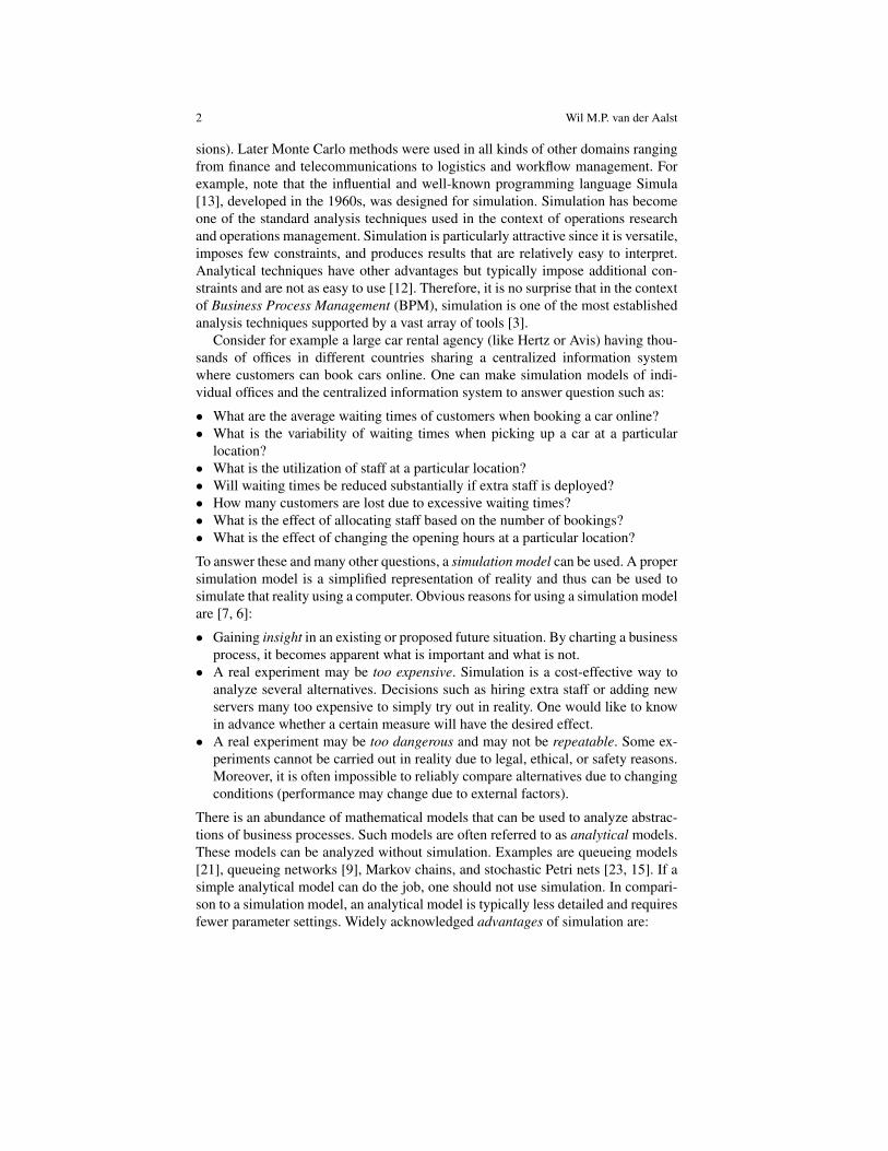
To explain the typical ingredients of a model used for business process simula-tion, we first focus on the control-flow of a business process. Figure 1 shows thesame control-flow using three widely used notations. Figure 1(a) shows a Petri net;a WF-net (WorkFlow net) to be precise [6, 17, 35]. Activities are modeled by labeledtransitions and the ordering of these activities is controlled by places (represented bycircles). A transition (represented by a square) is enabled if each of its input placescontains a token. An enabled transition may occur thereby consuming a token fromeach input place and producing a token for each output place. Initially, source placein contains a token. Hence, transition a is enabled in the initial state. After regis-tering a request (modeled by transition a), extra insurance can be added (b) or not(modeled by the silent transition). Then the check-in is initiated (c). Subsequently,the selection of the car (d), the checking of the license (e), and the charging of


the credit card ( f ) are executed (any ordering is allowed, including the concurrentexecution of d, e, and f ). Finally, the car is provided (g). The process instance ter-minates when place out is marked. Figure 1(b) shows an event log describing someexample traces.

BPMN, EPCs, UML ADs, and many other business process modeling notationshave in common that they all use token-based semantics. Therefore, there are manytechniques and tools to convert Petri nets to BPMN, BPEL, EPCs and UML ADs,and vice versa. As a result, the core concepts of Petri nets are often used indirectly,e.g., to enable analysis, to enact models, and to clarify semantics. For example,Figure 1(c) shows the same control-flow modeled using the Business Process Mod-eling Notation (BPMN). BPMN uses activities, events, and gateways to model thecontrol-flow. In Figure 1(c) two types of gateways are used: exclusive gatewaysare used to model XOR-splits and joins and parallel gateways are used to modelAND-splits and joins. BPMN also supports other types of gateways correspondingto inclusive OR-splits and joins, deferred choices, etc. [14, 17, 35]. Event-drivenProcess Chains (EPCs) use functions, events, and connectors to model the control-flow (cf. Figure 1(d)). Connectors in EPCs are similar to gateways in BPMN. Thereare OR, XOR, and AND connectors. Events in EPCs are similar to places in Petrinets. Just like places and transitions in a Petri net, events and functions need to al-ternate along any path in an EPC. However, events cannot have multiple successornodes, thus making it impossible to model deferred choices [17]. UML Activity Dia-grams (UML ADs) – not shown in Figure 1 – are similar to BPMN and EPCs whenit comes to the basic control-flow constructs.

b

add extra

insurance

initiate

check-in

e

check driver’s

license

f

charge credit

card

d

select car

provide

car

in

a c g

outregister

request

role A role B

simulation environment

arrival processsubrun

settingsselected KPIs

number of

resources per

role

resource

requirements

and usageresolution of

control-flow

choices (priorities

and probabilities)

activity duration

resolution of resource

choices (selection and

queueing discipline)

20%

80%

Fig. 2 Information required for business process simulation. This information is not needed forenactment (using for example a BPM/WFM system), but needs to be added for simulation.


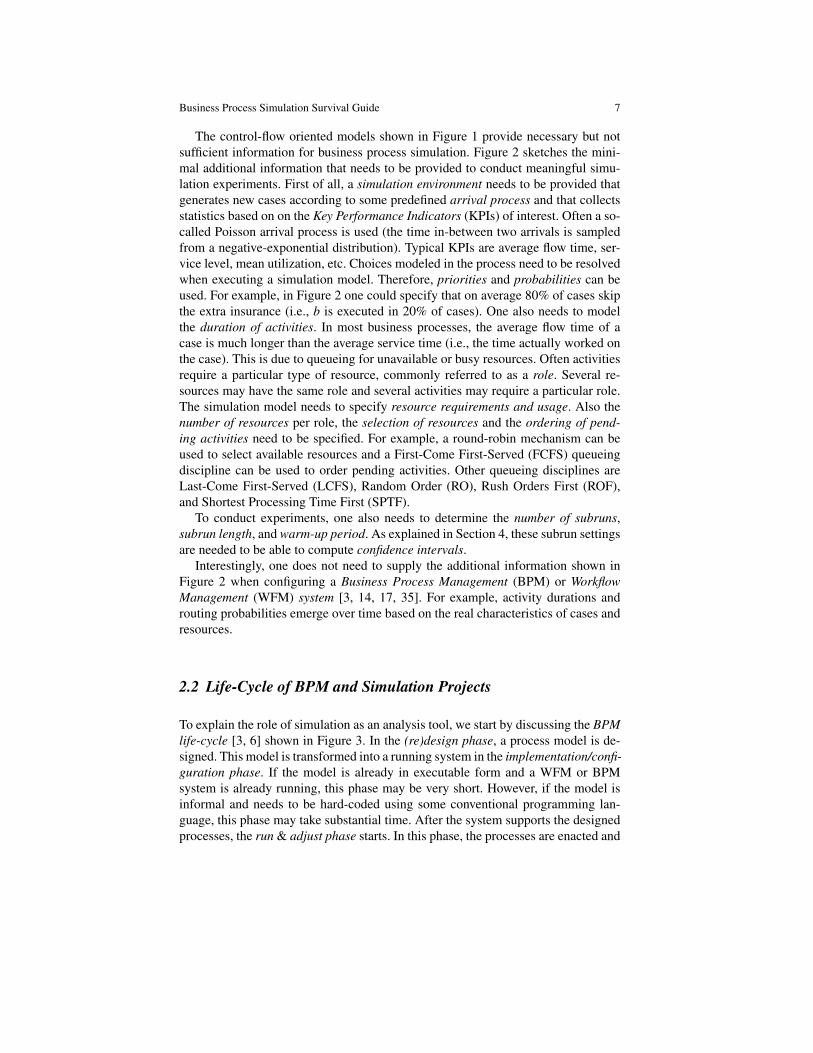
The control-flow oriented models shown in Figure 1 provide necessary but notsufficient information for business process simulation. Figure 2 sketches the mini-mal additional information that needs to be provided to conduct meaningful simu-lation experiments. First of all, a simulation environment needs to be provided thatgenerates new cases according to some predefined arrival process and that collectsstatistics based on on the Key Performance Indicators (KPIs) of interest. Often a so-called Poisson arrival process is used (the time in-between two arrivals is sampledfrom a negative-exponential distribution). Typical KPIs are average flow time, ser-vice level, mean utilization, etc. Choices modeled in the process need to be resolvedwhen executing a simulation model. Therefore, priorities and probabilities can beused. For example, in Figure 2 one could specify that on average 80% of cases skipthe extra insurance (i.e., b is executed in 20% of cases). One also needs to modelthe duration of activities. In most business processes, the average flow time of acase is much longer than the average service time (i.e., the time actually worked onthe case). This is due to queueing for unavailable or busy resources. Often activitiesrequire a particular type of resource, commonly referred to as a role. Several re-sources may have the same role and several activities may require a particular role.The simulation model needs to specify resource requirements and usage. Also thenumber of resources per role, the selection of resources and the ordering of pend-ing activities need to be specified. For example, a round-robin mechanism can beused to select available resources and a First-Come First-Served (FCFS) queueingdiscipline can be used to order pending activities. Other queueing disciplines areLast-Come First-Served (LCFS), Random Order (RO), Rush Orders First (ROF),and Shortest Processing Time First (SPTF).

To conduct experiments, one also needs to determine the number of subruns,subrun length, and warm-up period. As explained in Section 4, these subrun settingsare needed to be able to compute confidence intervals.

Interestingly, one does not need to supply the additional information shown inFigure 2 when configuring a Business Process Management (BPM) or WorkflowManagement (WFM) system [3, 14, 17, 35]. For example, activity durations androuting probabilities emerge over time based on the real characteristics of cases andresources.

2.2 Life-Cycle of BPM and Simulation Projects

To explain the role of simulation as an analysis tool, we start by discussing the BPMlife-cycle [3, 6] shown in Figure 3. In the (re)design phase, a process model is de-signed. This model is transformed into a running system in the implementation/confi-guration phase. If the model is already in executable form and a WFM or BPMsystem is already running, this phase may be very short. However, if the model isinformal and needs to be hard-coded using some conventional programming lan-guage, this phase may take substantial time. After the system supports the designedprocesses, the run & adjust phase starts. In this phase, the processes are enacted and


adjusted when needed. In the run & adjust phase, the process is not redesigned andno new software is created; only predefined controls are used to adapt or reconfigurethe process. Figure 3 shows two types of analysis: model-based analysis and data-based analysis. While the system is running, event data are collected. These datacan be used to analyze running processes, e.g., discover bottlenecks, waste, and de-viations. This is input for the redesign phase. During this phase process models canbe used for analysis. For example, simulation is used for “what if” analysis or thecorrectness of a new design is verified using model checking.

(re)

design

implement/configure

run & adjust

model-b

ased

analysis

data-based

analysis

Fig. 3 BPM life-cycle consisting of three phases: (re)design, implement/configure, and run &adjust. Traditional simulation approaches can be seen as a form of model-based analysis mostlyused during the (re)design phase.

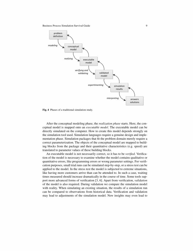
Traditionally, simulation is positioned on the left-hand side of Figure 3, i.e., busi-ness process simulation is a form of model-based analysis conducted during the(re)design phase. Figure 4 shows the phases of a typical simulation project. Thesephases should be seen as a further refinement of the (re)design phase in Figure 3.

The simulation process starts with a problem definition, describing the goals andfixing the scope of the simulation study. The scope tells what will and what willnot be a part of the simulation model. The problem definition should also state thequestions to be answered. Preferably, these questions should be quantifiable. Insteadof asking “Are the customers satisfied?”, one should ask “How long do customershave to wait on average?”

After defining the problem, the next phase is modeling. In this phase the con-ceptual model is created. The conceptual model defines classes of objects and therelations between these objects. In the case of a car rental organization exampleobjects to be distinguished are cars, customers, staff members, parking spaces, etc.The relevant characteristics (properties) of these objects need to be determined. Theconstruction of the conceptual model will most likely unveil incomplete and con-tradictory aspects in the problem definition. Also, the modeling process may bringforth new questions for the simulation study to answer. In either case, the problemdefinition should be adjusted.


conceptual model

problem definition

modeling

executable model

realizing

validated model

verifying and validating

simulation results

expertimenting

answers solutions

interpreting

Fig. 4 Phases of a traditional simulation study.

After the conceptual modeling phase, the realization phase starts. Here, the con-ceptual model is mapped onto an executable model. The executable model can bedirectly simulated on the computer. How to create this model depends strongly onthe simulation tool used. Simulation languages require a genuine design and imple-mentation phase. Simulation packages that fit the problem domain merely require acorrect parameterization. The objects of the conceptual model are mapped to build-ing blocks from the package and their quantitative characteristics (e.g. speed) aretranslated to parameter values of these building blocks.

An executable model is not necessarily correct, so it has to be verified. Verifica-tion of the model is necessary to examine whether the model contains qualitative orquantitative errors, like programming errors or wrong parameter settings. For verifi-cation purposes, small trial runs can be simulated step-by-step, or a stress test can beapplied to the model. In the stress test the model is subjected to extreme situations,like having more customers arrive than can be attended to. In such a case, waitingtimes measured should increase dramatically in the course of time. Some tools sup-port more advanced forms of verification [3, 6]. Apart from verification, validationof the model is also required. During validation we compare the simulation modelwith reality. When simulating an existing situation, the results of a simulation runcan be compared to observations from historical data. Verification and validationmay lead to adjustments of the simulation model. New insights may even lead to


adjusting the problem definition and/or the conceptual model. A simulation modelfound to be correct after validation is called a validated model.

Starting from the validated model, experiments can be carried out. These ex-periments have to be conducted in such a way that reliable results are obtained asefficiently as possible. In this stage decisions will be made concerning the numberof simulation runs and the length of each run (cf. Section 4).

The simulation results need to be interpreted to allow feedback to the problemdefinition. Confidence intervals will have to be calculated for the various KPIs basedon low-level measurements gathered during simulation. Also, the results will haveto be interpreted to answer the questions in the problem definition. For each suchanswer, the corresponding reliability should be stated. All these matters are sum-marized in a final report with answers to questions from the problem definition andproposals for solutions.

Figure 4 shows that feedback is possible between phases. In practice, manyphases do overlap. Specifically, experimentation and interpretation will often gohand in hand.

Figure 4 may be misleading as it refers to a single simulation model. Usually,several alternative situations are compared to one another. In that case, several sim-ulation models are created and experimented with and the results are compared.Often, several possible improvements of an existing situation have to be comparedthrough simulation. We call this “what if” analysis. Simulation is well-suited for“what if” analysis as it is easy to vary parameters and compare alternatives basedon selected KPIs.

3 Sampling from Distributions

Figure 2 illustrates that random variables need to be added to resolve choices, tosample durations from some probability distribution, and to generate the arrival ofnew cases. This section shows how to introduce “randomness” selectively.

3.1 Pseudo-Random Numbers

A simulation experiment is little more than replaying a modeled situation. To replaythis situation in computer, we have to make assumptions not only for the modeledbusiness process itself but also for its environment (cf. Figure 2). As we cannot orwill not model these matters in detail we turn to “Monte Carlo”. We do not knowwhen and how many customers will enter a car rental office, but we do know themean and variation of customer arrivals. So, we have the computer take seeminglyrandom samples from a probability distribution. The computer is by nature a deter-ministic machine, so we need to smartly generate so-called pseudo-random num-bers.


A random generator is a piece of software for producing pseudo-random num-bers. The computer does in fact use a deterministic algorithm to generate them,which is why they are called “pseudo random”. Most random generators generatepseudo-random numbers between 0 and 1. Each value between 0 and 1 being equallyprobable, these values are said to be distributed uniformly over the interval between0 and 1.

Most random generators generate a series of pseudo-random numbers Xim accord-

ing to the formula:Xn = (aXn−1 +b) modulo m

For each i, Xi is a number from the set {0,1,2, . . . ,m−1} and Xim matches a sample

from a uniform distribution between 0 and 1. The numbers a, b and m are chosen insuch a way that the sequence can hardly or not at all be distinguished from “trulyrandom” numbers. This means that the sequence Xi must visit, on average, each ofthe numbers 0,1,2, . . . ,m− 1 equally often. Also, m is chosen as closely as possi-ble to the largest integer that can be manipulated directly by the computer. Thereare several tests to check the quality of a random generator (cf. [11, 26, 34, 22]):frequency test, correlation test, run test, gap test and poker test.

A reasonable random generator for a 32-bit computer is:

Xn = 16807 Xn−1 modulo (231−1)

That is: a = 16807, b = 0 and m = 231−1. For a 64-bit machine:

Xn = (6364136223846793005 Xn−1 +1) modulo 264

is a good choice.The first number in the sequence (X0) is called the seed. The seed completely

determines the sequence of random numbers. In a good random generator, differentseeds produce different sequences. Sometimes the computer selects the seed itself(e.g., based on a system’s clock). However, preferably the user should consciouslyselect a seed himself, allowing the reproduction of the simulation experiment later.Reproducing a simulation experiment is important whenever an unexpected phe-nomenon occurs that needs further examination.

Today’s simulation tools provide adequate random generators. This generatorcan be seen as a black box: a device that produces (pseudo) random numbers uponrequest. However, beware: pseudo-random numbers are not truly random! (A deter-ministic algorithm is used to generate them.) Do not use more than one generatorand take care when selecting the seed.

To illustrate the dangers in using random generators we mention two well-knownpitfalls.

The first mistake is using the so-called ‘lower order bits’ of a random sequence.For example, if a random generator produces the number 0.1321734234, the higherorder digits 0.13217 are ‘more random’ than the lower order digits 34234. In generalthe lower order digits show a clear cyclical behavior.


Another frequent mistake is the double use of a random number. Suppose thatthe same random number is used twice for generating a sample from a probabilitydistribution. This introduces a dependency into the model that does not exist inreality, which may lead to extremely deceptive results.

3.2 Example Probability Distributions

Only rarely do we need random numbers uniformly distributed between 0 and 1. De-pending on the situation, we need samples from different probability distributions.A probability distribution specifies which values are possible and how probable eachof those values is.

To simplify the discussion of random distributions and samples from probabilitydistributions, we introduce the term random variable. A random variable X is avariable with a certain probability of taking on certain values. For example, we canmodel the throwing of a dice by means of a variable X that can take on the values 1,2, 3, 4, 5 and 6. The probability of obtaining any value a from this set is 1

6 . We canwrite this as follows:

IP[X = a] ={ 1

6 if a ∈ {1,2,3,4,5,6}0 else

Given a random variable X we can define its expectation and variance. The ex-pectation of X , denoted by IE[X ], is the average to be expected from a large numberof samples from X . We also say the mean of X . The variance, denoted as Var[X ], isa measure for the average deviation of the mean (expectation) of X . If X has a highvariance, many samples will be distant from the mean. Conversely, a low variancemeans that, in general, samples will be close to the mean. The expectation of a ran-dom variable X is often denoted with the letter µ , the variance (Var[X ]) is denotedas σ2. The relation between expectation and variance is defined by the followingequality:

Var[X ] = IE[(X−µ)2] = IE[X2]−µ2

As Var[X ] is the expectation of the square of the deviation from the mean, the squareroot of Var[X ] is a better measure for the deviation from the mean. We call σ =√

Var[X ] the standard deviation of X .Table 1, lists some well-known discrete probability distributions. For example,

a random variable X having a Bernoulli distribution with parameter p has two pos-sible values: 0 (no success) and 1 (success). Parameter p models the probability ofsuccess. Hence, IP[X = 1] = p. IE[X ] = p and Var[X ] = p(1− p).

Table 2 lists some continuous distributions. Unlike discrete distributions, theprobability of a specific value is zero, i.e., IP[X = k] = 0 for any k. Therefore, theprobability density function fX (k) is used to describe the likelihood of differentvalues. Consider for example a random variable X uniformly distributed on the in-


Table 1 Discrete random distributions.distribution domain IP[X = k] IE[X ] Var[X ]

Bernoulli

0≤ p≤ 1 k ∈ {0,1}{

1− p k = 0p k = 1 p p(1− p)

homogeneousa < b k ∈ {a, . . . ,b} 1

(b−a)+1a+b

2(b−a)((b−a)+2)

12binomial

0≤ p≤ 1 k ∈ {0,1, . . . ,n}(

nk

)pk(1− p)n−k n p n p(1− p)

n ∈ {1,2, . . .}geometric0≤ p≤ 1 k ∈ {1,2, . . .} (1− p)k−1 p 1

p1−pp2

Poissonλ > 0 k ∈ {0,1, . . .} λ k

k! e−λ λ λ

Table 2 Continuous random distributions.distribution domain fX (x) IE[X ] Var[X ]uniform

a < b a≤ x≤ b 1b−a

a+b2

(b−a)2

12exponentialλ > 0 x≥ 0 λe−λx 1

λ

1λ 2

normal

µ ∈ IR x ∈ IR 1√2πσ2 e

−(x−µ)2

2σ2 µ σ2

σ > 0gamma

r,λ > 0 x > 0 λ (λx)r−1 e−λx

Γ (r)rλ

rλ 2

Erlang

λ > 0 x > 0 λ (λx)r−1 e−λx

(r−1)!rλ

rλ 2

r ∈ {1,2, . . .}χ2 see gammav ∈ {1,2, . . .} x > 0 r = v

2 and λ = 12 v 2v

beta

a < b a≤ x≤ b 1b−a

Γ (r+s)Γ (r)Γ (s) a+(b−a) r

r+sr s(b−a)2

(r+s)2(r+s+1)

r,s > 0( x−a

b−a

)r−1 ( b−xb−a

)s−1

terval [a,b]. fX (k) = 1b−a , i.e., all values on the interval have the same likelihood.

IE[X ] = a+b2 and Var[X ] = (b−a)2

12 .Arrival processes are often modeled using the negative-exponential distribution.

Parameter λ is called the intensity of the arrival process, i.e., λ is the expectednumber of new arrivals per time unit. Negative-exponentially distributed randomvariable X models the time in-between two subsequent arrivals. IE[X ] = 1

λis the

expected average time between two such arrivals. If there is a large population of


potential cases (e.g., customers) that behave independently, then, by definition, theinter-arrival times are distributed negative exponentially. This is referred to as aPoisson arrival process.

Durations are often modeled using the normal or beta distribution. The well-known normal distribution has two parameters: µ (mean value) and σ (standarddeviation). If we use a normally distributed random variable for modeling time du-rations, like processing times, response times or transport times, we must be awarethat this random variable can also take on negative values. In general negative du-rations are impossible; this may even cause a failure of the simulation software.To circumvent this problem, we might take a new sample whenever the given sam-ple produces a negative value. Note that this will affect the mean and the variance.Therefore, this solution is recommended only if the probability of a negative value isvery small. We use the following rule of thumb: if µ−2σ < 0, the normal distribu-tion should not be used to model durations. The normal distribution with parametersµ = 0 and σ = 1 is called the standard normal distribution.

Like the uniform distribution, the beta distribution is distributed over a finiteinterval. We use it for random variables having a clear upper and lower bound.The beta distribution has four parameters a, b, r and s. The parameters a and brepresent the upper and lower bounds of the distribution. The parameters r (r > 0)and s (s > 0) determine the shape of the distribution. Very different shapes of theprobability density function are possible, see [7] for examples.

It is impossible to describe all frequently used probability distributions here.Probability distributions often used for simulation are described in detail in [7].Also consult standard textbooks on probability theory and simulation [8, 20, 22,26, 27, 30]. These references also explain how particular random variables can beconstructed from pseudo-random numbers. For example, if Xi is a pseudo randomnumber from the set {0,1, . . . ,m−1}, then −ln(Xi

m )/λ is a sample from a negative-exponential distribution with parameter λ .

4 Processing the Results

In Section 2.1 we described the typical ingredients of a simulation model. Sim-ulation models abstract from details that cannot be fully modeled (e.g., perfectlymodeling human decision making and customer behavior) or that are too specify(e.g., data entered into a form). Such abstractions may necessitate the introductionof stochastic elements in the model. For example, a path is selected with a certainprobability and the duration of an activity is sampled from some continuous proba-bility distribution. In Section 3 we showed that pseudo random numbers can be usedto introduce such stochastic elements. This section focuses on the interpretation ofthe raw simulation results. In particular, we will show that subruns are needed tocompute confidence intervals for KPIs.

During simulation there are repeated observations of quantities, such as wait-ing times, flow times, processing times, or stock levels. These observations pro-


vide information on KPIs (cf. Section 2.1). Suppose we have k consecutive obser-vations x1,x2, . . . ,xk also referred to as random sample. The mean of a number ofobservations is the sample mean. We represent the sample mean of observationsx1,x2, . . . ,xk by x. We can calculate the sample mean x by adding the observationsand dividing the sum by k:

x =∑

ki=1 xi

kThe sample mean is merely an estimate of the true mean. However, it is a so-calledunbiased estimator (i.e., the difference between this estimator’s expected value andthe true value is zero). The variance of a number of observations is the samplevariance. This variance is a measure for the deviation from the mean. The smallerthe variance, the closer the observations will be to the mean. We can calculate thesample variance s2 by using the following formula:

s2 =∑

ki=1(xi− x)2

k−1.

This is the unbiased estimator of the population variance, meaning that its expectedvalue is equal to the true variance of the sampled random variable.

In a simulation experiment, we can determine the sample mean and the samplevariance of a certain quantity. We can use the sample mean as an estimate for thereal expected value of this quantity (e.g., waiting time), but we cannot determinehow reliable this estimate is. The sample variance is not a good indicator for thereliability for the results. Consider for example the sample xa and sample variances2

a obtained from a long simulation run. We want to use xa as a predictor for someperformance indicator (e.g., waiting time). If we make the simulation experimentten times as long, we will obtain new values for the sample mean and the samplevariance, say, xb and s2

b, but these values do not need to be significantly differentfrom the previous values. Although it is reasonable to assume that xb is a morereliable predictor than xa, the sample variance will not show this. Actually, s2

b maybe greater than s2

a. This is the reason to introduce subruns.If we have n independent subruns, then we can estimate the reliability of es-

timated performance indicators. There are two approaches to create independentsubruns. The first approach is to take one long simulation run and cut this run intosmaller subruns. This means that subrun i+1 starts in the state left by subrun i. Asthe subruns need to be independent, the initial state of a subrun should not stronglycorrelate with the final state passed on to the next subrun. An advantage is that start-up effects only play a role in the first run. Hence, by inserting a single start run atthe beginning (also referred to as “warm-up period”), we can avoid incorrect conclu-sions due to start-up effects. The second approach is to simply restart the simulationexperiment n times. As a result, the subruns are by definition independent. A draw-back is that start-up effects can play a role in every individual subrun. Hence, onemay need to remove the warm-up period in all subruns.

There are two types of behavior that are considered when conducting simula-tion experiments: steady-state behavior and transient behavior. When analyzing the


(a) transient analysis (no warm-up period, initial state matters, bounded timeframe)

(b) steady-state analysis (separate runs each with warm-up period)

(c) steady-state analysis (long run with one warm-up period split into smaller subruns)

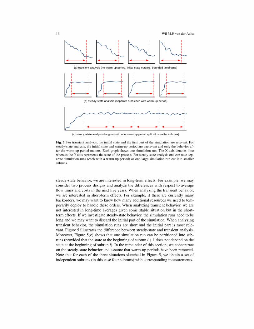
Fig. 5 For transient analysis, the initial state and the first part of the simulation are relevant. Forsteady-state analysis, the initial state and warm-up period are irrelevant and only the behavior af-ter the warm-up period matters. Each graph shows one simulation run. The X-axis denotes timewhereas the Y-axis represents the state of the process. For steady-state analysis one can take sep-arate simulation runs (each with a warm-up period) or one large simulation run cut into smallersubruns.

steady-state behavior, we are interested in long-term effects. For example, we mayconsider two process designs and analyze the differences with respect to averageflow times and costs in the next five years. When analyzing the transient behavior,we are interested in short-term effects. For example, if there are currently manybackorders, we may want to know how many additional resources we need to tem-porarily deploy to handle these orders. When analyzing transient behavior, we arenot interested in long-time averages given some stable situation but in the short-term effects. If we investigate steady-state behavior, the simulation runs need to belong and we may want to discard the initial part of the simulation. When analyzingtransient behavior, the simulation runs are short and the initial part is most rele-vant. Figure 5 illustrates the difference between steady-state and transient analysis.Moreover, Figure 5(c) shows that one simulation run can be partitioned into sub-runs (provided that the state at the beginning of subrun i+1 does not depend on thestate at the beginning of subrun i). In the remainder of this section, we concentrateon the steady-state behavior and assume that warm-up periods have been removed.Note that for each of the three situations sketched in Figure 5, we obtain a set ofindependent subruns (in this case four subruns) with corresponding measurements.


Suppose we have executed n subruns and measured a result yi for each subrun i.Hence, each result yi serves as an estimate for a performance indicator. We assumethat there exists a “true” value µ that each result yi approximates. We want to deriveassertions about µ from the values yi. For example, yi is the mean waiting timemeasured in subrun i and µ the “true” mean waiting time that we would find byconducting a hypothetical simulation experiment of infinite length. Also KPIs otherthan the mean waiting time could be considered, e.g., yi could be an estimate forthe mean variance of the waiting time, the mean occupation rate of a server, or themean length of a queue. However, we must be certain that the values yi are mutuallyindependent for all subruns. This can be ensured by choosing a long enough subrunlength or by using independent subruns. Given the results y1,y2, . . . ,yn, we derivethe sample mean:

y =∑

ni=1 yi

nand the sample variance:

s2y =

∑ni=1(yi− y)2

n−1.

The sample standard deviation is sy =√

s2y . The sample mean and the sample vari-

ance for the results of the subruns should not be confused with the mean and thevariance of a number of measures within one subrun. We can consider the sample yas an estimate of the true value µ . Value y can be seen as a sample from a randomvariable Y = (X1 +X2 + . . .+Xn)/n, the estimator. Now sy√

n is an indication of the

reliability of the estimate y. If sy√n is small, it is a good estimate.

If there is a large number of subruns, we can consider the estimator Y as nor-mally distributed. Here we use the well-known central limit theorem. For a setX1,X2, . . . ,Xn of independent uniformly distributed random variables with expec-tation µ and variance σ2, the random variable

(X1 +X2 + . . .+Xn)−nµ

σ√

n

converges for n→ ∞ to a standard normal distribution. Thus, the sum or averageof a large number of independent random variables is approximately normally dis-tributed. If the subrun results are indeed independent and there are plenty of suchresults, we can assume that the estimator Y is normally distributed. Therefore, wetreat the situation with over 30 subruns as a special case.

Given a large number of independent subruns (say, n≥ 30), we can easily deter-mine a confidence interval for the quantity to be studied. Because the sample meany is the average of a large number of independent measures, we can assume that y isapproximately normally distributed. From this fact, we deduce the probability thatthe true value µ lies within a confidence interval. Given the sample mean y and thesample standard deviation sy, the true value µ conforms with confidence (1−α) tothe following equation:


y−sy√

nz(

α

2)< µ < y+

sy√n

z(α

2)

where z(α

2 ) is defined as follows: If Z is a standard normally distributed randomvariable, then the probability that random variable Z is greater than z(x) is x. Table 3shows for five values of x the value z(x). The value α represents the unreliability;that is, the probability that µ does not conform to the equation. Typical values for α

range from 0.001 to 0.100. The interval[y−

sy√n

z(α

2),y+

sy√n

z(α

2)

]is known as the (1−α)-confidence interval for the estimated value µ .

Table 3 IP[Z > z(x)] = x where Z is standard normally distributed.

x z(x)0.001 3.0900.005 2.5760.010 2.3260.050 1.6450.100 1.282

Given a smaller number of independent subruns (say, n ≤ 30), we need to makemore assumptions about the distribution of the individual subrun results. A commonassumption is that the individual subrun results are normally distributed. This is arealistic assumption when the subrun result itself is calculated by taking the averageover a large set of independent measurements (see the central limit theorem, whichstates that as the sample size increases the distribution of the sample average of theserandom variables approaches the normal distribution irrespective of the shape of thecommon distribution of the individual terms). By using this assumption, we candeduce—given n subruns with a sample mean y, sample deviation sy, and reliability(1−α)—the following confidence interval:[

y−sy√

ntn−1(

α

2),y+

sy√n

tn−1(α

2)

]where tv(x) is the critical value of a Student’s t-distribution with v degrees of free-dom. Table 4 shows for several values of v and x the critical value tv(x).

Contrary to the method discussed earlier, we can now also determine the confi-dence interval if only a limited number of subruns (say, ten) is at our disposal. Forsmall numbers v, we have tv(x) > z(x). As v increases, the value of tv(x) decreasesand in the limit we obtain tv(x) = z(x).

When two confidence intervals are overlapping for a KPI, one cannot make anyfirm statements about the superiority of one the corresponding alternatives. More-


Table 4 The critical values for a Student’s t-distribution with v degrees of freedom.

tv(x) x =0.100 0.050 0.010 0.001

v = 1 3.08 6.31 31.82 318.312 1.89 2.92 6.96 22.333 1.64 2.35 4.54 10.214 1.53 2.13 3.75 7.175 1.48 2.02 3.37 5.896 1.44 1.94 3.14 5.217 1.41 1.89 3.00 4.798 1.40 1.86 2.90 4.509 1.38 1.83 2.82 4.30

10 1.37 1.81 2.76 4.1415 1.34 1.75 2.60 3.7320 1.33 1.72 2.53 3.5525 1.32 1.71 2.49 3.4550 1.30 1.68 2.40 3.26

100 1.29 1.66 2.35 3.17∞ 1.28 1.64 2.33 3.09

over, one alternative may score better with respect to costs whereas the other alter-native may reduce flow times significantly.

Using the above, we can compute confidence intervals for any KPI. If the confi-dence intervals are too wide, more subruns or longer subruns can be used to obtaintighter confidence intervals. As mentioned before, simulation is an excellent tool for“what if” analysis. Confidence intervals can be computed for different KPIs and dif-ferent alternatives. Alternatives can be created by varying parameters or by makingchanges in the design.

5 Pitfalls to Avoid

Simulation is a powerful and flexible tool that can be used to support decision mak-ing. If simulation is applied incorrectly (flawed model or poor analysis of the re-sults), then this may result in incorrect decisions that are very costly. Therefore, wepoint out 15 typical pitfalls of simulation that should be avoided. In Section 5.1 wepresent ten general risks that may result in incorrect conclusions and misleading in-sights. These are linked to the different phases of a simulation study (cf. Figure 6).Section 5.2 identifies five more specific risks caused by simulation models that donot incorporate essential phenomena such as working speeds depending on work-loads, partial availability of resources, and competition among activities in differentprocesses.


5.1 General Risks

In Section 2.2 we described the different phases of a traditional simulation study.Figure 6 lists ten risks pointing to typical errors (pitfalls) frequently made whenapplying simulation. These are described in the remainder.

conceptual model

problem definition

modeling

executable model

realizing

validated model

verifying and validating

simulation results

expertimenting

answers solutions

interpreting

Risk 1: One-sided problem definition

Risk 2: Wrong level of detail or scope

Risk 3: Hidden assumptions

Risk 4: Validation by the wrong people

Risk 5: Forcing the model to fit

Risk 6: Underexposure of the sensitivity of the model

Risk 7: No subruns

Risk 8: Careless presentation of the results

Risk 9: Dangers of animation

Risk 10: Unnecessary use of simulation

Fig. 6 Various risks associated to the different phases of a simulation study.

5.1.1 Risk 1: One-sided problem definition

A simulation study gets off on the wrong foot if the problem definition is drawnup exclusively by either the user or the systems analyst. The user may possess ex-tensive knowledge of the problem area, but lacks the experience needed for defininghis problem. The systems analyst on the other hand, fully knows the elements whichshould be present in a problem definition, but lacks the background of the specificproblem. The systems analyst is also aware of the possibilities and impossibilities ofsimulation. The user on the other hand, generally knowing little about simulation, isbarely informed on this issue. Therefore, for a simulation study to be successful, itis important that both parties closely cooperate in setting up the problem definition.The problem definition serves as a “contract” between the user and the builder ofthe model. Hence, the following rule of thumb should be used: “Do not start a sim-ulation study until it is clear to both user(s) and analyst(s) which questions need tobe answered!”.


5.1.2 Risk 2: Wrong level of detail or scope

In making a simulation model, one chooses a certain level of detail. In a simulationmodel for a manufacturing department, a machine may be modeled as an object witha mean service time as its only parameter. Alternatively, it can be modeled in detail,taking into account aspects such as set-up times, faults, tool-loading, maintenanceintervals etc. Many simulation studies end prematurely because a wrong level of de-tail is selected initially. Too much detail causes the model to become unnecessarilycomplex and introduces extra parameters that need to be assessed (with all the risksinvolved). Too many abstractions can lead to a simulation model that leaves the es-sential questions of the problem definition unanswered. The right level of detail ischosen if:

1. information is present that allows experiments with the model,2. the important questions from the problem definition are addressed by the model,

and3. the complexity of the model is still manageable for all parties concerned.

If it is impossible to choose a suitable level of detail satisfying these three condi-tions, the problem definition needs to be adjusted.

Related to the level of detail is the scope of the model. When analyzing a pro-cess handled within a department, one can also model the other processes within thesame department competing for the same resources and the other departments inter-acting with the process. One can think of the scope as the “breadth” of the modelwhereas the level of detail is the model’s “depth”. Broadening the scope or increas-ing the level of detail may lead to more accurate models. However, more detail or abroader scope may result in increased modeling and data gathering efforts. In fact,sometimes there is no data to support a more refined model. This is why probabilitydistributions are used.

The well-known “80/20-rule” also applies to simulation models: 80% of themodel’s accuracy is obtained from 20% of the model’s detail. Hence, a small in-crease in accuracy may require the addition of lots of details. Hence, the followingrule of thumb should be used: “Minimize the breadth and depth of a model given aset of predefined questions and required level of accuracy”.

5.1.3 Risk 3: Hidden assumptions

During modeling and while realizing an executable simulation model, many as-sumptions must be made. Assumptions are made to fill gaps in an incomplete prob-lem definition or because of a conscious decision to keep the simulation model sim-ple. Often these assumptions are documented poorly, if documented at all. Thesehidden assumptions may lead to the rejection of the simulation model during val-idation or later. Hidden assumptions may also lead to invalid conclusions and baddecisions. Therefore, all assumptions must be documented and regularly discussedwith the user.


5.1.4 Risk 4: Validation by the wrong people

Sometimes, due to time pressure or indifference of the user, the simulation model isonly validated by its maker(s). Discrepancies between the model and the ideas of theuser may thus be discovered too late, if at all. Therefore, the user should be involvedin the validation of the simulation model before any experiments are conducted.

5.1.5 Risk 5: Forcing the model to fit

In the validation phase, often the results of the simulation model do not match theobserved or recorded actual data. One is then tempted to make the model “fit” bychanging certain parameter values, i.e., the analyst fiddles around with the parametersettings until a match is found. This, however, is very dangerous, since this matchwith reality is most likely caused by sheer luck and not by a model that adequatelyreflects reality. Parameters should be adjusted only after having understood why themodel deviates from reality. This prevents the conscious or unconscious obscuringof errors in the model.

5.1.6 Risk 6: Underexposure of the sensitivity of the model

Certain model parameters (e.g. the intensity of the arrival process) are often set atone specific value. The chosen parameter settings should be justifiable. However,even if this is the case, small variations in the arrival process can have dramaticeffects.

Consider for example the M/M/1 queue describing the situation with a Pois-son arrival process (the inter-arrival times are distributed negative exponentially),negative-exponentially distributed service times and one server (i.e., at most onecustomer is served at a time). Assuming an arrival rate λ (average number of cus-tomers arriving per time unit) and service rate µ (average number of customers thatcan be handled per time unit), the average flow time is 1

µ−λ. If λ = 98 (on average

98 customers arrive per day) and µ = 100 (the average service time is approximately14 minutes), then the average flow time is 1

100−98 = 0.5 (12 hours). If λ increasesto 99 (an increase of approximately 1%), then the average flow time doubles to

1100−99 = 1, i.e., a full day. The example illustrates that a small increase in work-load may have dramatic effects on the mean flow or waiting time. Therefore, thesensitivity of the model to minor adjustments of its parameters should be seriouslyaccounted for.

5.1.7 Risk 7: No subruns

Some people say: “A sufficiently long simulation yields correct results!” They exe-cute a simulation run for a night or weekend and then blindly trust, e.g., the mean


waiting time measured. This is a very risky practice, as no assertions about the re-liability of the result can be given. Others derive a confidence interval from themean variance measured. This is also wrong because, for example, the mean vari-ance of the waiting time measured is unrelated to the reliability of the estimatedmean waiting time. The only way to derive independent measurements is by havingindependent subruns!

5.1.8 Risk 8: Careless presentation of the results

Interpreting the results of a simulation study may require complex statistical analy-ses. This is often a source of errors. Translating the results from statistics into lan-guage a user can understand, can be very tricky indeed. In Darrel Huff’s book “Howto lie with statistics” ([18]), there are numerous examples of sloppy and misleadingpresentations. As an example, suppose the final report of a simulation study containsthe following conclusion “Waiting times will be reduced by 10 percent”. This con-clusion is very incomplete, as it contains no reference whatsoever to its reliability.It is good practice to give a confidence interval. The same conclusion suggests thatwaiting times will be reduced by 10 percent for each customer. This, however, maynot be the case. The average waiting time may be reduced by 10 percent while itincreases for certain customers and is reduced somewhat more for others.

5.1.9 Risk 9: Dangers of animation

Modern simulation tools allow for impressive visualizations of simulation results.Animation facilities graphically show the process while it is unfolding. These facil-ities improve communication with the user. However, there is an inherent danger inanimation. As animation only shows the tangible aspects of the simulation model,the user may develop an unfounded faith in the model. The choice of parameters ordecision making rules deeply influence the simulation results, yet are barely visiblein an animation. The same hold for the presentation of simulation results. Impressive3D charts do not replace a sound statistical analysis.

5.1.10 Risk 10: Unnecessary use of simulation

Simulation is a flexible analysis tool that can be applied in almost any businesscontext. Therefore, one may be tempted to use it regardless of the circumstances.Often, however, a simple mathematical model (e.g. a queuing model) or a simplespreadsheet calculation is sufficient. In such cases simulation is “overkill”. It shouldonly be used if and when the situation requires it. Simulation is a means and not agoal!


5.2 Specific Risks

The ten risks highlighted in Figure 6 cover the different phases of a simulationproject. Besides these general risks there are more specific risks related to not in-corporating relevant contextual factors (that may be changing over time) and notcapturing characteristics of human resources (working patterns, partial availability,and varying working speeds). For example, human resources are typically modeledin a rather naı̈ve manner. As a result, it is not uncommon that the simulated modelpredicts flow times of minutes or hours while in reality flow times are weeks or evenmonths [5].

5.2.1 Risk 11: Abstracting away relevant contextual factors

Processes unfold in a particular context [29] that is often neglected in simulationstudies. Not capturing this context may result in simulation models with limitedpredictive value. To explain the notion of “context” consider Figure 7 (taken from[4]). In [4] four levels of context data are considered:

• Instance Context. Process instances (that is, cases) might have various propertiesthat influence their execution. Consider the way businesses handle a customerorder. The type of customer placing the order can influence the path the instancefollows in the process. The order’s size can influence the type of shipping thecustomer selects or the transportation time. These properties can directly relateto the individual process instance; we refer to them as the instance context. Typ-ically, discovering relationships between the instance context and the case’s ob-served behavior is not difficult. We might, for example, discover that an activityis typically skipped for VIP customers.

• Process Context. A process might be instantiated many times - for example, theprocess can handle thousands of customer orders per year. Yet, the correspondingprocess model typically describes one order’s life cycle in isolation. Although in-teractions among instances are not very explicit in most simulation models, theycan influence each other. Instances might compete for the same resources, and anorder might be delayed by too much work-in-progress. Looking at one instance inisolation is not sufficient for understanding the real behavior. Simulation modelsshould also consider the process context, such as the number of instances beinghandled and resources available for the process. When analyzing the flow time ofcases, the simulation model should consider not only the order’s status (instancecontext) but also the workload and resource availability (process context).

• Social Context. The process context considers all factors directly related to aprocess and its instances. However, people and organizations typically are notallocated to a single process and might be involved in many different processes.Moreover, activities are executed by people operating in a social network. Fric-tion between individuals can delay process instances, and the speed at whichpeople work might vary due to circumstances that are not fully attributable to the


instance

context

e.g. size of order or

type of customer

process context

social context

external context

e.g., number of resources

allocated to process, number

of cases in progress

e.g., prioritization over different

processes, social network,

stress levels, internal

competition

e.g., weather, economic

climate, seasonal effects,

changes in legislation

expanding scope (more instances,

more processes, etc.)

a more direct relationship

between cause and effect

Fig. 7 Levels of context data. Context can influence processes and may change over time. Never-theless, simulation models seldom explicitly model the outer two context levels and do not antici-pate context changes.

process being analyzed (see also Risk 14). We refer to all these factors as thesocial context, which characterizes how people work together within a particu-lar organization. Today’s simulation tools tend to neglect the social context eventhough it directly impacts how people and organizations handle cases.

• External Context. The external context captures factors that are part of an ecosys-tem that extends beyond an organization’s control sphere. For example, theweather, the economic climate, and changing regulations might influence howorganizations handle cases. The weather might influence the workload, as whena storm or flooding leads to increased insurance claims. Changing oil prices caninfluence customer orders, as when the demand for heating oil increases as pricesdrop. More stringent identity checks influence the order in which a governmentorganization executes social-security-related activities. Although external con-text can have a dramatic impact on the process being analyzed, selecting relevantvariables is difficult. Learning the external context’s effects is closely related toidentifying concept drift (see also Risk 12) - for example, a process might grad-ually change due to external seasonal effects.


Simulation models tend to focus on the first two levels of the “union model” depictedin Figure 7. This may be valid in many studies. However, if the social context andexternal context matter, they should be incorporated explicitly.

5.2.2 Risk 12: Ignoring concept drift

The term concept drift refers to a situation in which the process is changing whilebeing analyzed [10, 36]. Processes can change due to periodic or seasonal changes(“in December, there is more demand” or “on Friday afternoon, fewer employeesare available”) or to changing conditions (“the market is getting more competitive”).Such changes affect processes, and organizations must detect and analyze them. Thenotion of concept drift is closely related to the context notion illustrated in Figure 7.Large parts of the context cannot be fully controlled by the organization conduct-ing a simulation study. Therefore, contextual variability needs to be considered andcannot be ignored.

Predictable drifts (e.g., seasonal influences) with a significant influence on theprocess need to be incorporated in simulation models. For unpredictable drifts (e.g.,changing economic conditions), several “what if” scenarios need to be explored.

5.2.3 Risk 13: Ignoring that people are involved in multiple processes

In practice there are few people that only perform activities for a single process.Often people are involved in many different processes, e.g., a manager, doctor, orspecialist may perform tasks in a wide range of processes. The left-hand side ofFigure 8 shows a Gantt chart illustrating how an individual may distribute her timeover activities in different processes. Simulation often focuses on a single process,often ignoring competing processes.

Suppose a manager is involved in a dozen processes and spends about 20 percentof her time on the process that we want to analyze. In most simulation tools it isimpossible to model that she is only available 20 percent of the time. Hence, oneneeds to assume that the manager is there all the time and has a very low utilization.As a result the simulation results are too optimistic. In the more advanced simulationtools, one can indicate that resources are there at certain times in the week (e.g.,only on Monday morning). This is also an incorrect abstraction as the managerdistributes her work over the various processes based on priorities and workload.Suppose that there are 5 managers all working 20 percent of their time on the processof interest. One could think that these 5 managers could be replaced by a singlemanager (5*20%=1*100%). However, from a simulation point of view this is anincorrect abstraction. There may be times that all 5 managers are available and theremay be times that none of them is available.

People are involved in multiple processes and even within a single process dif-ferent activities and cases may compete for shared resources. One process may bemore important than another and get priority. In some processes cases that are de-


layed may get priority while in other processes late cases are “sacrificed” to finishother cases in time. People need to continuously choose between work-items and setpriorities. Although important, this is typically not captured by simulation models.

workload

sp

ee

d

optimal

stress level

overloaded

lethargic

activity A.1

activity A.2

…

activity A.8pro

ce

ss A

activity B.1

activity B.2

…

activity B.6pro

ce

ss B

activity C.1

activity C.2

…

activity C.9pro

ce

ss C

time

Fig. 8 People are typically involved in multiple processes and need to distribute attention overthese processes and related activities (left). Moreover, people do not work at constant speed (right).The “Yerkes-Dodson Law of Arousal” [37] describes the phenomenon that people work at differentspeeds based on their workload.

5.2.4 Risk 14: Assuming that people work at constant speeds

Another problem is that people work at different speeds based on their workload,i.e., it is not just the distribution of attention over various processes, but also theabsolute working speed that determines the resource’s contribution to the process.There are various studies that suggest a relation between workload and performanceof people. A well-known example is the so-called “Yerkes-Dodson Law of Arousal”[37]. The Yerkes-Dodson law models the relationship between arousal and perfor-mance as a ∩-shaped curve (see right-hand side of Figure 8). This implies that, fora given individual and a given type of task, there exists an optimal arousal level.This is the level where the performance has its maximal value. Thus work pressureis productive, up to a certain point, beyond which performance collapses. Althoughthis phenomenon can be easily observed in daily life [24], today’s business pro-cess simulation tools typically do not support the modeling of workload dependentprocessing times.

5.2.5 Risk 15: Ignoring that people work in batches

As indicated earlier, people may be involved in different processes. Moreover, theymay work part-time (e.g., only in the morning). In addition to their limited avail-abilities, people have a tendency to work in batches (cf. Resource Pattern 38: Piled


Execution [33]). In any operational process, the same task typically needs to beexecuted for many different cases (process instances). Often people prefer to letwork-items related to the same task accumulate, and then process all of these in onebatch. In most simulation tools a resource is either available or not, i.e., it is assumedthat a resource is eagerly waiting for work and immediately reacts to any work-itemthat arrives. Clearly, this does not do justice to the way people work in reality. Forexample, consider how and when people reply to e-mails. Some people handle e-mails one-by-one when they arrive while others process their e-mail at fixed timesin batch. Related is the fact that calendars and shifts are typically ignored in simu-lation tools. While holidays, lunch breaks, etc. can heavily impact the performanceof a process, they are typically not incorporated in the simulation model.

In [5] a general approach based on “chunks” is used to model availability moreadequately. The basic idea is that people spend “chunks of time” on a particularprocess or task. Within a period of time a limited number of chunks is available.Within a chunk, work is done in batches. As chunks become more coarse-grained,flow times go up even when the overall utilization does not change [5].

6 Advanced Simulation

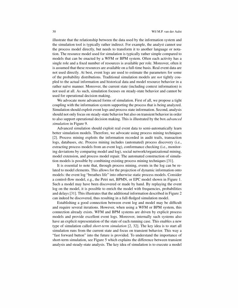
The 15 risks described in Section 5 illustrate that many things can go wrong in a sim-ulation project. Fortunately, modern IT infrastructures and the enormous amounts ofevent data collected in many organizations also enable new forms of simulation. ITsystems are becoming more and more intertwined with the business processes theyaim to support, resulting in an “explosion” of available data that can be used foranalysis purposes. Today’s information systems already log enormous amounts ofevents and it is clear that data-based analytics like process mining [2] will becomemore important. Increasingly, simulation techniques will need to incorporate actualevent data. Moreover, there will be a shift from off-line analysis at design time toon-line analysis at run-time.

Figures 2 and 4 present a rather classical view on business process simulation.This is the type of simulation supported by hundreds, if not thousands, of com-mercial simulation packages. Some vendors provide a pure simulation tool (e.g.,Arena, Extend, etc.) while others embed this in a workflow management system(e.g., FileNet, COSA, etc.) or a business process modeling tool (e.g., Protos, ARIS,etc.). All of these tools use the information presented in Figure 2 to simulate busi-ness processes and subsequently measure obvious performance indicators such asflow time, utilization, etc. Using Figure 9, we will show that it is possible to movebeyond “traditional” simulation approaches.

The left-hand-side of Figure 9 shows the role of a process-aware informationsystem (a WFM/BPM system or any other process-oriented information system,e.g., an ERP system like SAP) in supporting operational business processes. Theinformation system supports, controls, and monitors operational processes. The re-sources within the organization perform tasks in such processes and therefore also


information

system

operational process

organization/

resources

process model

real event data

process state

resource model

describe

configure

interact

record

use

traditional simulation (steady state, naive view of

resources, only indirect use of

historic information)

advanced simulation (transient and steady state,

refined view of resources, use

of historic and state information)

enactment analysissimulation

report

simulated event

data

unified view on

simulated and

real event data

Fig. 9 Advanced simulation compared to traditional simulation. Note that real event data andsimulated event data can be stored in event logs and analyzed using the same process miningtool. Due to this unified view on process behavior, simulation can be embedded in day-to-daymanagement and decision making.

interact with the information system. The information system can only do meaning-ful things if it has knowledge of the process, the resources within the organizationand the current states of active cases. Moreover, today’s information systems oftenrecord historical information for auditing and performance analysis. The lower fourellipses in the middle of Figure 9 show four types of data implicitly or explicitlyavailable when an information system is supporting an operational process: (1) realevent data, (2) process state, (3) process model, and (4) resource model. An eventlog (i.e., real event data) contains historical information about “When, How, and byWhom?” in the form of recorded events. The process state represents all informationthat is attached to currently running cases, e.g., Customer order XYZ consists of 25order lines and has been in the state “waiting for replenishment” since Monday. Theprocess state may also contain context information relevant for the process, e.g.,the weather or economic trends. The process model describes the ordering of tasks,routing conditions, etc. The resource model holds information about people, roles,departments, etc. Clearly, the process state, process model, and resource model maybe used to enact the process. The event log merely records the process as it is actu-ally enacted.

The right-hand-side of Figure 9 focuses on analysis rather than enactment; itlinks the four types of data to simulation. For traditional simulation (i.e., in thesense of Figures 2 and 4) a hand-made simulation model is needed. This simula-tion model can be derived from the process model used by the information system.Moreover, information about resources, arrival processes, processing times, etc. isadded (cf. Figure 2). The arcs between the box traditional simulation and the threetypes of data (real event data, process model, and resource model) are curved to


illustrate that the relationship between the data used by the information system andthe simulation tool is typically rather indirect. For example, the analyst cannot usethe process model directly, but needs to transform it to another language or nota-tion. The resource model used for simulation is typically rather simple compared tomodels that can be enacted by a WFM or BPM system. Often each activity has asingle role and a fixed number of resources is available per role. Moreover, often itis assumed that these resources are available on a full-time basis. Real event data arenot used directly. At best, event logs are used to estimate the parameters for someof the probability distributions. Traditional simulation models are not tightly cou-pled to the actual information and historical data and model resource behavior in arather naı̈ve manner. Moreover, the current state (including context information) isnot used at all. As such, simulation focuses on steady-state behavior and cannot beused for operational decision making.

We advocate more advanced forms of simulation. First of all, we propose a tightcoupling with the information system supporting the process that is being analyzed.Simulation should exploit event logs and process state information. Second, analysisshould not only focus on steady-state behavior but also on transient behavior in orderto also support operational decision making. This is illustrated by the box advancedsimulation in Figure 9.

Advanced simulation should exploit real event data to semi-automatically learnbetter simulation models. Therefore, we advocate using process mining techniques[2]. Process mining exploits the information recorded in audit trails, transactionlogs, databases, etc. Process mining includes (automated) process discovery (i.e.,extracting process models from an event log), conformance checking (i.e., monitor-ing deviations by comparing model and log), social network/organizational mining,model extension, and process model repair. The automated construction of simula-tion models is possible by combining existing process mining techniques [31].

It is essential to note that, through process mining, events in the log can be re-lated to model elements. This allows for the projection of dynamic information ontomodels: the event log “breathes life” into otherwise static process models. Considera control-flow model, e.g., the Petri net, BPMN, or EPC model shown in Figure 1.Such a model may have been discovered or made by hand. By replaying the eventlog on the model, it is possible to enrich the model with frequencies, probabilitiesand delays [31]. This illustrates that the additional information described in Figure 2can indeed be discovered, thus resulting in a full-fledged simulation model.

Establishing a good connection between event log and model may be difficultand require several iterations. However, when using a WFM or BPM system, thisconnection already exists. WFM and BPM systems are driven by explicit processmodels and provide excellent event logs. Moreover, internally such systems alsohave an explicit representation of the state of each running case. This enables a newtype of simulation called short-term simulation [2, 32]. The key idea is to start allsimulation runs from the current state and focus on transient behavior. This way a“fast forward button” into the future is provided. To understand the importance ofshort-term simulation, see Figure 5 which explains the difference between transientanalysis and steady-state analysis. The key idea of simulation is to execute a model


repeatedly. The reason for doing the experiments repeatedly, is to not come up withjust a single value (e.g., “the average response time is 10.36 minutes”) but to provideconfidence intervals (e.g., “the average response time is with 90 percent certaintybetween 10 and 11 minutes”). For transient analysis the focus is on the initial partof future behavior, i.e., starting from the initial state the “near future” is explored.For transient analysis the initial state is very important. If the simulation starts in astate with long queues of work, then in the near future flow times will be long and itmay take quite some time to get rid of the backlog. For steady-state analysis the ini-tial state is irrelevant. Typically, the simulation is started “empty” (i.e., without anycases in progress) and only when the system is filled with cases measurement starts.Steady-state analysis is most relevant for answering strategic and tactical questions.Transient analysis is most relevant for operational decision making. Lion’s share ofcontemporary simulation support aims at steady-state analysis and, hence, is limitedto strategic and tactical decision making. Short-term simulation focuses on opera-tional decision making; starting from the current state (provided by the informationsystem) the “near future” is explored repeatedly. This shows what will happen if nocorrective actions are taken. Moreover, “what if” analysis can be used to explorethe effects of different interventions (e.g., adding resources and reconfiguring theprocess).

Figure 9 shows that advanced simulation uses all information available, e.g.,event data to learn process characteristics, the current state to enable short-term sim-ulation (“fast forward button”), and a more refined resource model to better captureworking patterns.

Process mining techniques are driven by event logs recorded for the actual pro-cess. Similar event logs can be generated by simulation. In both cases events aredescribed by a reference to some process instance (the case), an activity, a times-tamp, a resource, and other attributes (e.g., costs). The top-most ellipse in the middleof Figure 9 (tagged “simulated event data”) refers to event logs produced by simu-lation rather than reality. As shown, both simulated and real events can be viewedusing the same tools. This is very important for operational decision making and“what if” analysis. Different future scenarios can be explored using visualizationsalso used for past and current event data.

7 Conclusion

This chapter provides a “survival guide” to business process simulation. Besidesproviding a basic introduction to the topic, the chapter lists 15 risks, i.e., potentialpitfalls, when using simulation. Moreover, the chapter also shows that more ad-vanced forms of simulation come into reach as IT and business processes get moreintertwined.

To conclude the chapter, we suggest books and articles for BPM academics andprofessionals that want to learn more about business process simulation:


• There are many (text) books on simulation, see for example [8, 11, 16, 19, 20, 22,25, 26, 27, 28, 30, 34]. Books like [20, 27, 30] focus on the statistical aspects ofsimulation. Books like [8, 19, 16, 22] focus on the creation of simulation models.The book “Successful Simulation: A Practical Approach to Simulation Projects”[28] is one of the few books focusing on simulation projects (including topicssuch as project management).

• In [15, 23] various techniques for the analysis of stochastic Petri nets (i.e., Petrinets extended with priorities, probabilities, and durations) are described. See [9,12, 21] for some seminal papers on the analysis of processes using analyticalmethods.

• For more information on role of various analysis techniques (including simula-tion) in BPM we refer to [3, 6, 14, 17, 35]. See [2, 31] for techniques to auto-matically discover simulation models from event data and [32] for operationaldecision support using simulation (e.g., short-term simulation).

This chapter is based on [1, 4, 5, 7]: in [1] we elaborate on the relation betweensimulation and process mining, in [5] we focus on the proper modeling of resourceavailability, in [4] we emphasize the importance of incorporating context, and in [7]we provide a tutorial on conventional business process simulation.

Acknowledgements. The author would like to thank Joyce Nakatumba, MarcVoorhoeve, Anne Rozinat, Ronny Mans, Hajo Reijers, Michael Westergaard, andMariska Netjes for their joint work on business process simulation. This workwas supported by the Basic Research Program of the National Research UniversityHigher School of Economics (HSE).

References

1. W.M.P. van der Aalst. Business Process Simulation Revisited. In J. Barjis, editor, Enter-prise and Organizational Modeling and Simulation, volume 63 of Lecture Notes in BusinessInformation Processing, pages 1–14. Springer-Verlag, Berlin, 2010.

2. W.M.P. van der Aalst. Process Mining: Discovery, Conformance and Enhancement of Busi-ness Processes. Springer-Verlag, Berlin, 2011.

3. W.M.P. van der Aalst. Business Process Management: A Comprehensive Survey. ISRN Soft-ware Engineering, pages 1–37, 2013. doi:10.1155/2013/507984.

4. W.M.P. van der Aalst and S. Dustdar. Process Mining Put into Context. IEEE Internet Com-puting, 16(1):82–86, 2012.

5. W.M.P. van der Aalst, J. Nakatumba, A. Rozinat, and N. Russell. Business Process Simula-tion: How to Get it Right? In J. vom Brocke and M. Rosemann, editors, Handbook on Busi-ness Process Management, International Handbooks on Information Systems, pages 313–338.Springer-Verlag, Berlin, 2010.

6. W.M.P. van der Aalst and C. Stahl. Modeling Business Processes: A Petri Net Oriented Ap-proach. MIT press, Cambridge, MA, 2011.

7. W.M.P. van der Aalst and M. Voorhoeve. Simulation Handbook. BPM Center Report BPM-00-04, BPMcenter.org, 2000. (Original Dutch version appeared as “W.M.P. van der Aalst.Handboek Simulatie. Computing Science Reports 95/32, Eindhoven University of Technol-ogy, Eindhoven, 1995”).


8. T. Altiok and B. Melamed. Simulation Modeling and Analysis with Arena. Elsevier AcademicPress, Amsterdam, 2007.

9. F. Baskett, K.M. Chandy, R.R. Muntz, and F.G. Palacios. Open, Closed and Mixed Networksof Queues with Different Classes of Customers. Journal of the Association of ComputingMachinery, 22(2):248–260, April 1975.

10. R.P. Jagadeesh Chandra Bose, W.M.P. van der Aalst, I. Zliobaite, and M. Pechenizkiy. Han-dling Concept Drift in Process Mining. In H. Mouratidis and C. Rolland, editors, Interna-tional Conference on Advanced Information Systems Engineering (Caise 2011), volume 6741of Lecture Notes in Computer Science, pages 391–405. Springer-Verlag, Berlin, 2011.

11. P. Bratley, B.L. Fox, and L.E. Schrage. A Guide to Simulation. Springer-Verlag, Berlin, 1983.12. J.A. Buzacott. Commonalities in Reengineered Business Processes: Models and Issues. Man-

agement Science, 42(5):768–782, 1996.13. O.J. Dahl and K. Nygaard. SIMULA: An ALGOL Based Simulation Language. Communica-

tions of the ACM, 1:671–678, Sept 1966.14. M. Dumas, M. La Rosa, J. Mendling, and H. Reijers. Fundamentals of Business Process

Management. Springer-Verlag, Berlin, 2013.15. P.J. Haas. Stochastic Petri Nets: Modelling, Stability, Simulation. Springer Series in Opera-

tions Research. Springer-Verlag, Berlin, 2002.16. A.K. Hartmann. Practical Guide to Computer Simulations. World Scientific Publishing,

Singapore, 2009.17. A.H.M. ter Hofstede, W.M.P. van der Aalst, M. Adams, and N. Russell. Modern Business

Process Automation: YAWL and its Support Environment. Springer-Verlag, Berlin, 2010.18. D. Huff. How to Lie With Statistics. Penguin Books, New York, 1954.19. D.W. Kelton, R. Sadowski, and D. Sturrock. Simulation with Arena. McGraw-Hill, New York,

2003.20. J. Kleijnen and W. van Groenendaal. Simulation: A Statistical Perspective. John Wiley and

Sons, New York, 1992.21. L. Kleinrock. Queueing Systems, Vol. 1:Theory. Wiley-Interscience, London, 1975.22. A.M. Law and D.W. Kelton. Simulation Modeling and Analysis. McGraw-Hill, New York,

1982.23. M. Ajmone Marsan, G. Balbo, G. Conte, S. Donatelli, and G. Franceschinis. Modelling with

Generalized Stochastic Petri Nets. Wiley series in parallel computing. Wiley, New York, 1995.24. J. Nakatumba and W.M.P. van der Aalst. Analyzing Resource Behavior Using Process Mining.

In S. Rinderle-Ma, S. Sadiq, and F. Leymann, editors, BPM 2009 Workshops, Proceedings ofthe Fifth Workshop on Business Process Intelligence (BPI’09), volume 43 of Lecture Notes inBusiness Information Processing, pages 69–80. Springer-Verlag, Berlin, 2010.

25. T.H. Naylor, J.L. Balintfy, D.S. Burdick, and Kong Chu. Computer Simulation Techniques.Wiley, New York, 1966.

26. M. Pidd. Computer Modelling for Discrete Simulation. John Wiley and Sons, New York,1989.

27. B. Ripley. Stochastic Simulation. Wiley-Interscience, Hoboken, USA, 2006.28. S. Robinson. Successful Simulation: A Practical Approach to Simulation Projects. McGraw-

Hill, Maidenhead, UK, 1994.29. M. Rosemann, J. Recker, and C. Flender. Contextualisation of Business Processes. Interna-

tional Journal of Business Process Integration and Management, 3(1):47–60, 2008.30. S.M. Ross. A Course in Simulation. Macmillan, New York, 1990.31. A. Rozinat, R.S. Mans, M. Song, and W.M.P. van der Aalst. Discovering Simulation Models.

Information Systems, 34(3):305–327, 2009.32. A. Rozinat, M. Wynn, W.M.P. van der Aalst, A.H.M. ter Hofstede, and C. Fidge. Workflow

Simulation for Operational Decision Support. Data and Knowledge Engineering, 68(9):834–850, 2009.

33. N. Russell, W.M.P.van der Aalst, A.H.M. ter Hofstede, and D. Edmond. Workflow ResourcePatterns: Identification, Representation and Tool Support. In O. Pastor and J. Falcao e Cunha,editors, Proceedings of the 17th Conference on Advanced Information Systems Engineering(CAiSE’05), volume 3520 of Lecture Notes in Computer Science, pages 216–232. Springer-Verlag, Berlin, 2005.


34. R.E. Shannon. Systems Simulation: The Art and Science. Prentice-Hall, Englewood Cliffs,1975.

35. M. Weske. Business Process Management: Concepts, Languages, Architectures. Springer-Verlag, Berlin, 2007.

36. G. Widmer and M. Kubat. Learning in the Presence of Concept Drift and Hidden Contexts.Machine Learning, 23:69–101, 1996.

37. R.M. Yerkes and J.D. Dodson. The Relation of Strength of Stimulus to Rapidity of Habit-Formation. Journal of Comparative Neurology and Psychology, 18:459–482, 1908.

Business Process Simulation Survival Guide - TU/ewvdaalst/publications/z8.pdf · Business Process...

Documents

Transcript of Business Process Simulation Survival Guide - TU/ewvdaalst/publications/z8.pdf · Business Process...