Business location and spatial externalities: Tying ...sweeney/Sweeney_Feser_SISS_chapter.pdfBusiness...

Business location and spatial externalities:Tying concepts to measures

Stuart H. Sweeney†

University of California at Santa Barbara

and

Edward J. Feser‡

University of North Carolina at Chapel Hill

June 2002

The research reported in this paper was supported by grants from the National Science Foundation (BCS-9986541)and the Center for Spatially Integrated Social Sciences at UC Santa Barbara. Data are used with special permissionfrom the US Bureau of Labor Statistics (BLS). Research results and conclusions expressed are the authors’ and donot necessarily indicate concurrence by the BLS. We would like to thank Rick Clayton, Mike Searson, Tim Pivetzand Holly Olson for providing access to the BLS data and supporting our research. We also thank Henry Renski forassistance with data preparation and to Art Getis for access to his point pattern analysis program for generating thelocal-G(s) statistics.

† Assistant Professor, Department of Geography, Ellison Hall 3611, University of California, Santa Barbara, CA93106-406, Voice: (805) 893-5647, Fax: (805) 893-3146, Email: [email protected]

‡ Assistant Professor, Department of City and Regional Planning, CB 3140, New East Building, University of NorthCarolina, Chapel Hill, NC 27599-3140, Voice: (919) 962-4768, Fax: (919) 962-5206, Email: [email protected]


ABSTRACTSpatial externalities among businesses, though notoriously difficult to measure, are a centralconcern in urban and regional economics. Traditionally they–along with closely related conceptssuch as agglomeration economies–have been studied empirically with hedonic models,production and cost functions, and simplified growth models. More recently, researchers havebegun using direct measures of proximity among businesses to shed light on the influence ofexternalities on industrial location, regional growth, and localized technological change. Theshift has been aided by an explosion in spatially-referenced economic data, advances in spatialstatistics, and the advent of affordable and user-friendly GIS and related software.

As existing indicators of concentration and spatial association have been adapted for theeconomic domain and new ones developed, the pool of measures useful for business locationresearch generally, and externalities more specifically, has expanded. In this paper, wesystematically review and compare a set of leading indicators of business co-location usingstandard data sets and evaluation criteria. Ultimately, our aim is to assess the capabilities andlimits of the measures for understanding spatial business externalities. More generally, wediscuss a number of common challenges associated with drawing inferences from cross-sectionalspatial data.

3


INTRODUCTIONThe notion that firms enjoy inherent and significant benefits from co-location is both intuitively

persuasive and empirically challenging. Positive spatial business externalities (or localized

business spillovers) are cost savings or productivity benefits that accrue to firms as a direct result

of their geographic proximity to other businesses. Such externalities are a source of increasing

returns, which help explain sustained economic growth in endogenous growth models, the

geographical concentration of industrial activity, the ability of some regions to buck convergence

and maintain dominant economic positions vis-á-vis other regions, and patterns of intraregional

and international trade. Business externalities and spillovers are the subject of considerable

research of late and are at the core of an emerging field that spans geography and economics (the

so-called new economic geography; see Clark, Feldman, and Gertler 2000).

Business externalities, which may not be reflected in prevailing prices (i.e., they can be

either pecuniary or non-pecuniary in nature), generally derive from access to a productive factor,

technology, or innovation. For example, companies in a given region benefit from pools of

skilled and unskilled labor that are jointly attracted and sustained by neighboring businesses.

They may also benefit from ready access to plentiful input supplies or producer services and

faster rates of innovation diffusion and information sharing (so-called knowledge spillovers).

Closely related is the concept of an agglomeration economy, a notion which encompasses

benefits from interfirm proximity (termed localization economies) as well as general advantages

associated with the size of urban areas (termed urbanization economies). The dimension of

accessibility behind spatial business externalities was largely viewed in terms of distance and

scale (a large number of tightly co-located businesses were presumed to enjoy more externalities

than a fewer number of more dispersed firms) early in the urban and regional economics

literatures. More recently, researchers have emphasized the nature of the conduits via which

localized business and labor interactions flow, including prevailing social and cultural norms,

regulatory frameworks, contracting practices within commodity chains, and important

intermediary institutions such as universities and colleges, government laboratories, and

4

employment agencies. There is strong evidence that such factors heavily mediate the influence

of geographic proximity on business cost, productivity, and innovation.

Externalities are notoriously difficult to measure and existing research is only partially

successful in isolating their practical significance and character. The most common empirical

approaches include the use of regional cost and production functions, hedonic pricing models,

simplified growth models, models of technology adoption and diffusion, and models of regional

wage and amenity differentials (Feser 1998, Hanson 2000). More recently, researchers have

turned to the analysis of the spatial distribution of employment and businesses as a means of

quantifying externalities and increasing returns. Such work is propelled by the increasing

availability of economic data at higher levels of geographic resolution as well as rapid

developments in spatial statistics, geocomputation, and related software. Research in the

strategic management literature that links industry co-location to national and international

economic competitiveness under the rubric of industry clusters has also been influential (e.g.,

Porter 1990, 2000). Indeed, a massive applied and academic literature on industry clusters has

developed as cities, regions, and states around the world have sought to exploit cluster concepts

in their own development strategies and policies (Steiner 1998; Roelandt and den Hertog 1999;

Bergman, Charles, and den Hertog 2001).

If positive business externalities truly reduce costs or improve productivity, they should

be detectable either directly with applied production models and methods or indirectly via

observed regional differences in wages, growth rates, and innovation rates. Positive externalities

should also encourage firms to concentrate or cluster geographically, ceteris paribus, as firms

take the benefits of co-location into account in their location decisions. It is this last sort of

evidence that we are chiefly concerned with here. Spatial proximity among businesses may also

generate negative externalities, which will offset positive effects to some degree. In the end,

spatial business externalities may be positive or negative in the net, leading to spatial

concentration or dispersion. In the agglomeration economies literature, the notion of net

economies drives empirical models of optimal city size.

The paper is concerned chiefly with revealed industry location as a source of evidence of

externalities. We begin by developing a map of the conceptual domain of spatial externalities, in

a sense establishing “bounds” on the notion of a spatial economic cluster as a theoretical

5

construct. Establishing those bounds permits an assessment of the construct validity of

competing measures of business co-location. We then undertake a kind of controlled comparison

of a set of such measures using micro data for selected industries in Los Angeles and Atlanta.

From the baseline data, which are point referenced, we construct three spatial resolutions of areal

data to look for differences among the measures as the scale of the analysis changes. The

objective of the comparison is not to analyze the Los Angeles and Atlanta economies per se, but

rather to assess the variation in results generated by the indicators. A small (large) variation in

the findings suggests that differences in the conceptual validity of the measures is small (large).

The paper closes with a general assessment of the measures, a summary of unresolved

methodological issues, and recommendations for future research.

More generally, the problems that surround the current state of empirical measurement of

externalities are illustrative of a set of common challenges that face attempts to draw inferences

about socio-economic spatial behavior from cross-sectional areal data. In principle, spatial

externalities, like many other behavioral phenomena of interest to geographers and regional

scientists, are best studied with dynamic models and time-series methods and data. However,

appropriate models and methodologies are in their infancy and time-series data with sufficient

geographic resolution, while improving, remain severely limited. Researchers are heavily

dependent on areal data in particular, which are ordinarily only indirectly representative of the

phenomena under study, usually in cross-sections. As a result, strong assumptions are generally

required to draw inferences. Over time, as those assumptions are invoked repeatedly in

numerous studies, they are often subject to less and less scrutiny. By revisiting the assumptions

and approaches common to the study of one particular area of study, business externalities, we

hope to contribute to a better understanding of the strengths and limitations of cross-sectional

areal analysis more broadly.

RELATING CONCEPTS TO MEASURESLong-standing academic and policy interest in spatial business externalities has yielded a large

literature on the topic. Although the conceptual terrain has clearly advanced from decades of

work, the literature is also characterized by significant redundancy among core concepts. Much

of the current literature has its origins in Marshall (1920). We will not attempt to review those

6

conceptual roots here both because it would take us too far afield and because there are extensive

reviews already available (Feser 1998, Gordon and McCann 2000). The goal of this paper is to

consider the value of co-location measures that have or might be employed to empirically

evaluate the concept of spatial business externalities.

For social scientific research to be of value, theory and measurement must proceed in

balance. Elaborate theorizing is vacuous if it fails to produce empirically-testable hypotheses.

Similarly, blind empiricism in the absence of theory yields only meaningless arrays of disjointed

facts. The domain of research design concerned with maintaining that balance is measurement

theory and, more specifically, the concept of construct validity. The criterion of construct

validity is highly pragmatic: it is the evaluation of operationalized measures based on whether

they measure the concepts they purport to measure. According to Trochim (2001, p. 64),

construct validity allows one to assess the, “degree to which inferences can legitimately be made

from the operationalizations in [the] study to the theoretical constructs on which those

operationalizations are based.”

The notion of construct validity provides a useful framework for evaluating the relative

utility of geographic measures of business location–including simple concentration measures and

indicators of spatial association–for understanding business externalities. A particularly relevant

type of construct validity is content validity, or the degree to which an operational measure

matches the full conceptual domain of the pertinent construct (i.e., “the extent to which a

measure adequately measures all facets of a concept,” Singleton et al., 1988, p. 118). Content

validity is described by Trochim (2001) as a kind of translation validity, where the latter is

concerned with how the construct is translated into an operationalization. Put differently, a good

measure is one that reflects all critical dimensions of the concept in question.

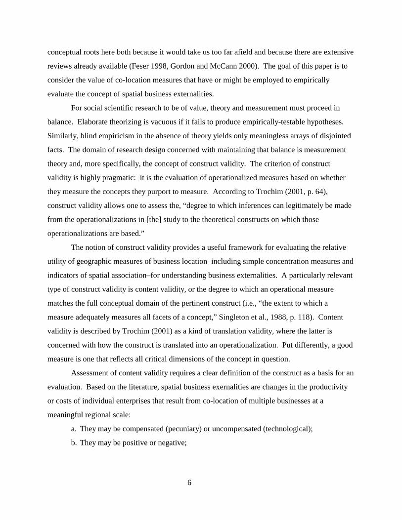
Assessment of content validity requires a clear definition of the construct as a basis for an

evaluation. Based on the literature, spatial business exernalities are changes in the productivity

or costs of individual enterprises that result from co-location of multiple businesses at a

meaningful regional scale:

a. They may be compensated (pecuniary) or uncompensated (technological);

b. They may be positive or negative;

7

c. They may accrue during a single time period, or over multiple time periods

with increasing or decreasing effect;

d. They may accrue to all industries in a location, to a single industry, or to a

subset of linked or related industries;

e. They derive not from scale or size per se (the number of establishments or

volume of production in a place) but from changes in the organization of work

and division of labor that business co-location (and implied increasing scale)

permits;

f. They originate from different sources (e.g., shared infrastructure, labor pools,

knowledge spillovers), and resulting business concentration or dispersion may

be realized for different spatial scales, types of industries, and forms of

business organization (small firms, large firms, singly-owned versus multi-

establishment businesses, vertically versus horizontally integrated companies,

and so on);

g. Their spatial and temporal extensiveness may depend on several factors

including:

• The nature of the local institutional and regulatory environment;

• Prevailing social and cultural norms;

• The character of industrial organization in a place;

• Regional and urban spatial structure.

Measures of business co-location have the potential to shed light on the dimensions of the

externalities concept that are identified in italics. But there are two significant challenges for

researchers working along these lines. The first is that the identification of spatial clustering (or

dispersion) alone says nothing about whether businesses derive cost or productivity advantages

(or disadvantages) from co-location. Clustering or dispersion itself is not evidence of spatial

externalities; natural resource or transportation advantages (harbors, canals, rail, roads),

accessibility to sources of demand (population concentration), and simple dumb luck followed by

historical lock-in effects can easily explain observed patterns of industrial concentration (Ellison

and Glaeser 1997). Dispersion might be explained by explicit market and pricing strategies or

the distribution of natural resources. The relative utility of geographic measures of business

1 First and second order properties of a spatial process are akin to the first and secondmoment terminology common to basic statistics. With spatial processes it desirable to removethe dependence of the mean and covariance on the size of spatial units by rescaling to per unitarea measures. The first order properties describe the mean number of events per unit area andthe second order properties describe the dependence between events in to different areas.

8

location for understanding externalities turns on whether they can accommodate those alternative

explanations.

The second major challenge is that the range, or spatial scale, over which such

externalities are likely to operate is not uniform. In general, one would expect that some types of

cross-business interactions generate externalities at the scale of neighborhoods or small districts

while others are binding at the level of the regional labor market or metropolitan area. Since the

issue of scale is an open empirical question, the best co-location measures will admit inspection

over a range of scales. To complicate matters, the scale of externality effects will likely vary

among industries and metropolitan areas according to differences in industrial organization,

urban form, and institutional structure. The ideal measure would admit controls for

characteristics of establishments and the overall spatial structure of the built environment.

These two challenges can be summarized as follows: observed business concentrations

or spatial clusters (or patterns of dispersion) are both time- and place-dependent. Relative

location is an important determinant of development. Some areas are climatically or geologically

blessed and the values attached to those blessings change over time. In short, historical processes

leave a footprint on the spatial structure of cities and regions. Any cross-sectional snapshot of a

city will reveal the aggregate impact of past industrial location decisions. In assessing business

spatial externalities, we must separate such historical processes from the interactions among

industries that drive business locations in the current period. In terms of measurement that

means that the optimal data and measures would emerge from longitudinal data that record

observed location decisions over several periods. In the absence of such data, measures should

isolate the second-order characteristics (or covariance) of the location process from the first-order

(or mean).1

Alternative Measures

2 The industry co-location measures in the lower right quadrant of Table 1 are membersof a large family of measures designed to assess distributional differences. Common applicationsare to income inequality (Gini and Theil) and residential segregation. The coefficient oflocalization of regional science is identical to the dissimilarity index of the sociology literature. A small sociology literatures assesses the construct validity of such measures. Excellent reviewsinclude Allison (1978), Massey and Denton (1988), and White (1983). The comparison ofdistributions dates back to work by Pearson (1895), Lorenz (1905), Gini (1914), and Yntema(1933), among others.

9

Table 1 partitions several potential business co-location measures according to the nature of their

input data and treatment of space. The indicators use either point data, which reveal the exact

locations of establishments, or areal data, which effectively aggregate points into spatial zones

and thereby impose the assumption that externalities operate at a scale at least as large as the

spatial unit of analysis (e.g., zip codes, counties, metro areas, or states). Area-based measures

have been used most extensively to study business co-location since establishment-level data are

rare. Some of the indicators use space explicitly in the form of distances or a contiguity matrix,

while others simply treat it as a nominal regional identifier. Each has already been used in

research on business externalities and industry clustering (indicated in bold face type) or falls

into a general class of indicators potentially useful for such research. In the discussion that

follows, we focus on the former, each of which is defined formally in Table 2. Our concern is

with the content validity of the measures; details of their statistical properties are available

elsewhere (Cliff and Ord 1973, Ripley 1977, Getis 1984, Diggle and Chetwynd 1991, Getis and

Ord 1992, Ord and Getis 1995, Ellison and Glaeser 1997).

[Table 1 and 2 near here]

Area data, implicit treatment of space. The measures with the weakest content validity

are those in the lower right quadrant of Table 1. They use areal data but do not explicitly account

for spatial proximity. Instead, they effectively assign area labels as a categorical variable,

characterizing differences in distributions over the areal labels between an industry of interest

and a referent group.2 The three measures which have been used to examine industry co-location

are the coefficient of localization (dating back to Hoover’s work on the shoe industry; Hoover

1948), location quotients, and Ellison’s and Glaeser’s ! (1997). The coefficient of localization is

simply the halved sum of absolute differences between a subregional industry share and a

subregional total employment share, where the shares are with respect to some referent region.

3 An additional problem with any measures that use subregional shares is that thevariance over the set of regions is heteroskedastic, as noted by Besag and Newell (1991). Thismeans that small population areas may register high values, thus making large contributionstowards concentration, even when the underlying probability of locating in the given area is equalto larger population areas.

10

The ! is effectively a coefficient of localization that incorporates information about the size

distribution of the industry via a Herfindahl index. Both the coefficient of localization and ! take

low values when the industry distribution and referent distributions are similar and high values

when the distributions are dissimilar. Dissimilarity is interpreted as concentration, though as we

will see below, the interpretation is opaque since either positive or negative distributional

deviations yield high values.3

Area data, explicit treatment of space. Among area-based co-location measures, the

most theoretically appealing are those that incorporate space explicitly either as intercentroid

distances or as a contiguity matrix (lower left quadrant in Table 1). Such measures have

traditionally been the workhorses of social science research on spatial processes, again mainly

because the bulk of available data is area-based. Ord and Getis (1995) and Anselin (1995) both

make a distinction between global and local measures. Global measures of spatial

autocorrelation attempt to measure second-order properties of a spatial pattern. The second order

interactions are measured slightly differently in these measures. Both the Moran’s I and Geary’s

c rely on deviations from means whereas Getis and Ord’s G uses cross-products.

The local statistics of spatial autocorrelation, termed LISAs by Anselin, have been

proposed as a means to identify “hot spots” or pockets of spatial autocorrelation.

Computationally, this is accomplished by parsing out the contribution of each areal unit to the

overall global statistic. Maps of the values can then be used to locate important pockets of

spatial interaction. An example of an industrial location application is Feser, Sweeney, and

Renski (2001). The advantage of the LISAs is that it is often relevant to both determine whether

business clustering exists over some threshold and to identify the number and precise location of

such clusters. Conceptually, the local statistics are an important adjunct to other indicators of

spatial clustering and dispersion.

Getis and Ord’s-G can also be used for areal data where distances are constructed from

the centroids of the areal units. The measure reports positive values for clustering and negative

4 The validity of areal co-location measures increases as the spatial scale of the datadecreases, although there is an exception to the rule for measures using shares since the pointestimates of those shares are less stable at smaller spatial scales.

5 Simpson’s paradox is the name commonly applied to such aggregation inducedreversals.

11

values for dispersion. This contrasts with the Moran’s-I or Geary’s-c, where either high or low

values both imply positive spatial autocorrelation. The G also produces values over a range of

scales down to a minimum scale equal to the size of the basic areal unit of analysis.4 As a

content valid indicator of externalities, G(s) therefore fares better than other spatially explicit

areal measures and is far superior to the spatially inexplicit metrics.

A major shortcoming of all areal measures is that they obscure the underlying location

pattern through spatial aggregation and the imposition of arbitrary administrative boundary

definitions. Spatial aggregation is problematic since the rank order of results may shift or reverse

at different levels of aggregation.5 Moreover, the results may also change under different

boundary definitions. This is the modifiable areal unit problem (MAUP). Although the

influence of aggregation and boundary definitions on results is certainly an undesirable property,

social scientists are often forced to work with areal data.

Another problem is that areal data necessarily impose a minimum spatial scale over

which clustering can be observed. Although region-scale industry clustering, say at the

metropolitan level, may be of academic or policy interest in some cases, its relevance to spatial

externalities as a theoretical construct is questionable. One can make a strong case that some

types of inter-business interaction that drive externalities would likely take place at a sub-

metropolitan, or even sub-county, scale. An example is the exchange of informal or tacit

knowledge between firms that yields productivity increases or other improvements in business

performance. There is even less relevance to the state scale, which has actually been studied

most extensively (particularly in the agglomeration economies literature) since data are readily

available. Redressing or solving such problems requires either pure point data (business

locations coded to street address) or synthetic point data (business locations at very small

geographic scales such as zip codes or Census tracts).

6 Complete spatial randomness (CSR) describes a process that distributes events in spacesuch that the mean number of events per unit area is constant. CSR is usually characterized by ahomogeneous Poisson process with a constant parameter, ".

12

Point data, explicit treatment of space. The measures contained in the upper left

quadrant of Table 1 utilize the most detailed spatial data and distance formulations. Ripley

(1977) is credited with developing the K-function, the first distance-based second-moment

measure in spatial statistics. As with all of the measures in the upper left quadrant, the K-

function indicates the degree of spatial clustering or dispersion over a range of distances, s. As

noted above, this is one of the desired properties of a measure since the range of clustering (or

dispersion) is something that can only be assessed empirically, though we may have hypotheses

about relevant scales from theory. The various measures in the quadrant differ mainly in terms of

the referent used to assess whether a pattern is clustered or dispersed. Both the K-function and

Getis and Ord’s G (used with point data) employ complete spatial randomness as the referent.6

Strictly speaking, that means that the measures only yield valid results when they are used to

assess spatial patterns where there is no large scale (first-order) variation in the mean of the

process. Otherwise, the first- and second-order properties of the spatial pattern are confounded

in the measurement. That is clearly not desirable in the business location context since all human

settlements are characterized by first-order variation; that is, we observe cities and towns in any

region and employment districts in any metropolitan area. Since Getis and Ord’s G allows for

the use of positive rational numbers as weights, it is possible to partially account for such first-

order variation (Feser, Sweeney, and Renski 2001).

The D-function, in contrast, was explicitly designed to measure clustering in the presence

of first-order variation (Diggle and Chetwynd 1991). The D-function is constructed as the

difference between two K-functions, one of which measures the second-order properties of a

subpopulation of interest (“cases”) and the other of which measures the second-order properties

of a random sample of objects from the general population (“controls”). The D-function

indicates whether a subpopulation is more or less clustered (i.e., dispersed) than the overall

clustering (or dispersion) in the population as a whole.

Of all the measures in Table 1, the D-function–which is really more of a methodological

framework than an individual measure–exhibits the most content validity with respect to the

13

measurement of business externalities. First, the control group provides a means of capturing the

general spatial structure of a given city or region. Second, stratified random sampling can assure

that the control group matches the case group along certain confounding dimensions (Sweeney

and Feser 1998, Feser and Sweeney 2000, 2001a, 2001b). Third, the D-function takes advantage

of the rich spatial detail inherent in point data and therefore can search over various spatial

scales. Fourth, the framework has an intuitively appealing economic interpretation. If one views

industry locations as choices on an unobserved spatially-continuous profit surface, the control

group may be viewed as characterizing the general properties of the profit surface faced by all

firms while the case group reveals the attributes unique to that reduced set of industries. In an

agglomeration economies context, the control group might be thought of as measuring

urbanization economies, in which case the D-function itself identifies the increment in clustering

associated with localization economies (Feser and Sweeney 2000). It is important to note that

there is no reason why the control framework of the D-function could not also be applied to G(s).

Employed in the same way, the D-function and G(s) should yield similar results.

An Empirical AssessmentIf we had outside information about the precise pattern of clustering (or dispersion) of businesses

in a given location, as well as the degree to which externalities played a role in generating the

observed spatial pattern, we could formally evaluate the performance and accuracy of the co-

location measures. Absent such information, we conduct a kind of controlled comparison to

assess the variation in substantive findings yielded by the measures as well as illustrate their

interpretation. By “controlled” comparison, we mean the use of point data that can be aggregated

to standardized areal units of our choosing (e.g., grids) so that we can generate findings at

different scales for both the area and point-based measures.

Our data are the street address and total employment of business establishments in six

manufacturing industries in Atlanta and Los Angeles, as reported in the U.S. Bureau of Labor

Statistics’ confidential ES-202 files. The industries–electronics, textiles and apparel, motor

vehicles, petrochemicals, aerospace, and publishing–were selected to include both high tech and

traditional manufacturing activity. Details of the procedures and success rates of matching ES-

202 addresses to approximate latitude and longitude coordinates are reported elsewhere (Feser

7Of course, other measures are also possible (e.g., output, value-added, wages, etc.). However, employment and establishments dominate applications to date.

14

and Sweeney 2002a). Briefly, the ES-202 file contains employment and payroll data for all

businesses subject to employment security law, an estimated 90 percent of U.S. firms. It

excludes sole proprietorships. For 1997, the year used in this analysis, some 65 percent of ES-

202 records contain physical addresses. We were able to establish longitude and latitude

coordinates for over 70 percent of those records in Atlanta and Los Angeles, yielding a net match

rate of 46 percent. In other words, we were able to locate nearly half of business units in the six

industries in the two study regions, a substantial sample size in industry location analysis by

conventional standards. Sample bias is modest. It is mainly associated with location; address

match rates are lower in the fastest growing or more rural parts of the metro areas. To minimize

the problem, we focus on a reduced core area of the two cities by drawing a box that captures the

major clusters of industries when we plot the locations of all manufacturers. In general, however,

bias is a minimal concern in the current application since our purpose is primarily to assess the

variation in findings across measures rather than to study the Los Angeles and Atlanta economies

per se.

An important question is the appropriate indicator of economic activity. Cases have been

made in the literature for both establishments and employment.7 Some of the measures, e.g.,

D(s) and G(s), will work for establishments or employment while others, such as !, are restricted

to examining employment. The case for employment rests primarily on the notion that size is an

important barometer of concentration or clustering, i.e., that a couple of firms with 10,000

employees apiece constitutes a more significant concentration of activity than 10 firms with 15

employees apiece. Establishments, on the other hand, are the principal units between which

externality-inducing interactions are likely to occur (implying that the more enterprises in a given

place, the more likely they are to enjoy positive externalities based on co-location). In the

absence of a compelling argument excluding either approach, we calculate the results using both

employment and establishments where possible.

We aggregated the point data set to three levels: a 2 kilometer resolution, a 5 kilometer

resolution, and a 10 kilometer resolution. We then used the point data set and three sets of areal

data to calculate the point- and area-based co-location measures. Before comparing results,

8 The point map is only an approximate simulation based on the areal data. Our data useagreement with the Bureau of Labor Statistics forbids us from publishing the real point map.

15

several visualizations of the data help set the stage by identifying the location and frequency of

manufacturing clusters.

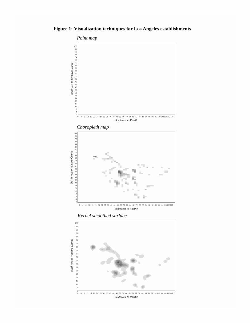
Visualizing industry location. Figure 1 displays three visualizations of manufacturing

locations in Los Angeles: a point map, a choropleth map, and a kernel smoothed map. The point

and basic choropleth maps are the simplest means of characterizing the general spatial pattern of

manufacturing establishments in Los Angeles.8 However, they suffer from too much and too

little detail, respectively. The lower panel of Figure 1 is generated by applying kernel smoothing

techniques, developed for bivariate statistical distributions, and then mapping the results. The

kernel smoothed images identify three, or perhaps four, centers of manufacturing activity in the

study region. The images can be altered based on the properties of the kernel smoothing

algorithm and the number of bins used to map colors onto the map. Appendix 1 contains several

versions of kernel smoothed images for the six study industries in the two cities.

[Figure 1 near here]

Figure 2 displays choropleth maps of the local G for manufacturing establishments in the

two study cities. The maps are more granular than the kernel images but also easily identify the

same centers. There are two advantages of the G over the kernel smoothers. First, the local G

can be calculated over different spatial scales resulting in different images, a process roughly

akin to altering the bandwidth in the kernel smoothing algorithm. Thus the results can be used to

investigate a series of prior beliefs about the nature and scale of business clustering. Second, the

local G is scaled in standard scores (Z-scores) so statistical significance of the mapped clusters

can also be assessed. In this application using the underlying 2 kilometer resolution data, we

chose a 5 kilometer scale of influence. Los Angeles, somewhat unexpectedly given its reputation

for sprawl, displays a very prominent central cluster with perhaps two subordinate centers,

whereas Atlanta displays three dominant manufacturing centers.

[Figure 2 near here]

Figures 3a and 3b display choropleth maps of the local G for establishments for the six

study industries in the two cities. The maps are suggestive of general tendencies towards

concentration or deconcentration and provide some insight to the location and frequency of

9 Employment size quantiles are used to construct the Herfindahl component of the !index ( in Table 2).

16

clusters. In Los Angeles for example (Figure 3a), both textiles/apparel and publishing are highly

concentrated. In contrast, the motor vehicles industry is at the other end of the spectrum with a

fairly diffuse pattern. Both aerospace and electronics are clustered in locations away from the

central core of the city, with the electronics located in a dominant node in the San Fernando

valley. The contrast between Los Angeles and Atlanta is also striking. In Atlanta, the electronics

industry is more centralized, with both a single node and a location near the city center. Textiles

and apparel manufacturing, in contrast, is more dispersed in Atlanta than Los Angeles.

[Figures 3a and 3b near here]

Aggregate tendencies towards clustering/dispersion. Though the visual depiction of

business locations is useful as a starting point, aggregate measures that characterize the spatial

pattern of economic activity in terms of statistically significant clustering or dispersion, as well

as provide a means of assessing the influences behind the observed pattern (such as externalities),

have considerable advantages. In this section we interpret and compare findings generated with

four co-location measures–D(s), G(s), the coefficient of localization (COL), and !–for both

establishment counts and employment.

Table 3 reports COL results based on three spatial grids (2, 5, and 10 kilometer). Results

for the ! statistic are provided over the same range of spatial scales (2, 5, and 10 kilometer grids)

in Table 4.9 Recall from the discussion above that ! is defined only for employment counts

while COL can be calculated for both establishments and employment.

For establishments, the COL takes the highest values in both cities for the aerospace and

motor vehicles industries. The rankings for employment are similar though aerospace slips to

third in Los Angeles at the two and five kilometer resolutions. The lowest values are posted for

publishing and electronics in Atlanta and textiles and electronics in Los Angeles. Strictly

speaking, high values of the COL indicate only a deviation from the baseline distribution (all

manufacturing employment or establishments). If the baseline is relatively clustered, then any

distribution either more clustered or more dispersed will yield high values for the index. Motor

vehicles likely generates a high value because it is more dispersed than the baseline (contrast the

17

patterns for motor vehicles in Figures 3a and 3b with the overall manufacturing patterns in Figure

2). In general, the ambiguity of the results means that collateral information is needed to

determine whether the measure is indicative of dispersion or clustering.

The high COL for aerospace (and highest ! for all spatial scales in both cities) reflects a

more serious problem with the two measures. The explanation is that aerospace is a

comparatively small industry in both places (relative to the other five study sectors) and the

employment, or establishment, surface contains a large number of zero cells. In the abstract, this

means that even if an industry locates in a region according to the exact same probability surface

shared by other industries, an industry with a small number of establishments will register a

higher index value (either LOC or !) because of the zero cells. More generally, this relates to

the problem noted by Besag and Newell (1991) that small populations in cells have higher

variances that lead to spurious results. This problem is alleviated by using higher levels of

spatial aggregation; higher cell counts essentially stabilize the cell proportions. But increased

spatial aggregation mitigates against detecting spatial clustering or dispersion at the smaller

geographical scales appropriate for testing hypotheses about externalities.

[Tables 3 and 4 near here]

There are two other noteworthy aspects of the findings in Tables 3 and 4. First, the rank

orderings shift over the three spatial scales. For example, using !, the Los Angeles textiles and

apparel sector is tied for 3rd at the 2 kilometer resolution, and shifts to 2nd at both the 5 and 10

kilometer resolutions. That the textiles and apparel sector could be ranked either 2nd or 3rd is

surprising given the visual dominance of that sector in Figure 3a (as we will see below both G(s)

and D(s) functions detect that dominance). While most of the rank shifts are slight, they

illustrate the effects of the modifiable areal unit problem nonetheless: the ordering of results

depends on both the size and configuration of the areal units. It follows that the results from

applied business cluster studies that use administrative boundaries to define the spatial polygons

are suspect since the scale of observations will often vary at both intra- and inter-metropolitan

scales.

Second, the ! is extremely sensitive to the choice of quantile used to construct the

Herfindahl index. As noted above, Ellison’s and Glaeser’s ! metric is a function of the

Herfindahl index which evaluates an industry’s size distribution as the sum of squared inverse

18

proportions of industry employment in a given employment size quantile. The columns of Table

4 contain the results of evaluating ! using 5, 20, 100, and then observation-wise quantiles to

construct the Herfindahl. For many choices, the !, which is only defined for positive values,

takes negative values, thereby rendering the metric uninterpretable.

Illustrative results for the global G(s) and D(s) are shown in Figure 4. A complete set of

figures showing the results for all industries, both metropolitan areas, and for both establishments

and employment are available on the web site associated with this book. Note that for G(s), the

value for total employment is included as a reference. Also, recall that the referent for G(s) is

complete spatial randomness whereas D(s) employs a case-control framework. In Figure 4, the

dashed horizontal lines at approximately 2 and -2 indicate confidence bands. Reading from left

to right the path traced by G(s) or D(s) indicates the degree of spatial clustering at the scale

indicated by the kilometers on the horizontal axis. The G(s) has a minimum scale imposed by

the 2-km grid resolution. The results are similar but do lead to qualitatively different

interpretations. Though textiles shows clear indications of strong spatial clustering, the results

for electronics and aerospace are at odds with each other.

Overall, the findings for complete set of G(s) and D(s) statistics are roughly in accord

with the visualizations. In Los Angeles, textiles is most clustered followed by publishing and

then petrochemicals. The electronics industry shows some significant clustering at a small

spatial scale (<5 kilometers). Motor vehicles, as anticipated, is most dispersed (even statistically

significantly dispersed at a small spatial scale). For Atlanta, both publishing and electronics are

identified as the most clustered, though aerospace is identified as more dispersed than vehicle

manufacturing. In comparison to the total employment G(s) values, only the textiles and apparel

sectors in Los Angeles indicate some clustering in excess of the general spatial pattern of

establishments in the study region.

In short, G(s) provides subjectively appealing rankings but cannot answer the question

that D(s) is constructed to answer: is the observed clustering beyond the general level of

establishments in the region? Moreover, the G(s) does not control for any of the confounding

factors associated with business location decisions. As discussed above, the case-control

framework of D(s) employs stratified proportionate sampling to construct a control group of

industries that match the ‘case’ industry sectors’ attributes associated with location decisions. In

10 The method of identifying outliers is discussed elsewhere (Feser and Sweeney 2001a,Sweeney and Feser 2001). The results with the outliers included can be viewed at the web siteassociated with this book.

19

theory, the framework produces two sets of sample industry locations such that the industries in

the two samples only differ along a single dimension of interest. The hypothesis test simply

evaluates whether the observed differences in spatial patterns are significantly different. For

example, one facet of the localization economies notion could be tested by identifying “case”

industries that share intermediate input suppliers and a set of controls that match the case

industry attributes except for their connectivity in input suppliers space. In practice, the stratified

sampling is limited by scope of variables in a data set.

[Figures 4 near here]

The D(s) results are constructed using establishments in an industry group (e.g.,

electronics) as the cases and a proportionately employment-size distribution matched sample of

controls from the rest of the population of manufacturing establishments. We also use a

supplemental set of analyses to identify and remove industry sectors with extreme leverage on

the results of D(s), parallel to the concept of outlier observation detection in regression.10 It is

clear that the D(s) generates richer information about clustering and dispersion than the other

measures. For example, in both Atlanta and Los Angeles, the estimated D(s) for establishment

counts reveals high levels of clustering in the aerospace industry at very small spatial scales (<2

km). Petrochemicals displays a similar pattern in Atlanta. For employment in Atlanta, the

variation in D(s) over the range of spatial scales is even more pronounced. Moreover, by

construction, D(s) indicates clustering or dispersion in excess of the background population. The

dispersion evident in the visualizations for the motor vehicles industry in both Los Angeles and

Atlanta is shown to be broadly characteristic of the overall spatial pattern of establishments in

each study region; that is, the spatial pattern of establishments of motor vehicles is statistically

insignificant (neither clustered nor dispersed).

It is difficult to assess the general pattern of results across all of the measures from the

separate graphs and tables. Tables 5 and 6 summarize the findings by assigning ranks assigned

11 It is somewhat problematic assigning a single rank to the results of D(s) and G(s) sincethe rankings change over the range of scales. In the tables, the rankings for D(s) and G(s) arebased on small scale orderings (<5 kilometers).

20

by each of the four measures.11 The results for Los Angeles (see Table 5) clarify some of the

points made above. The first three orderings for the establishment G(s) and D(s) are identical but

the measures disagree on the pattern for electronics. The establishment-based industry rankings

for the COL make little sense as noted above. The employment-based industry rankings show

less agreement between G(s) and D(s), especially with regard to aerospace. For the Atlanta

employment-based results, aerospace and vehicles are ranked 1st and 2nd by G(s), COL, and !

while D(s) ranks the same two industries, respectively, as dispersed and insignificant. It is

difficult to say why G(s) and D(s) disagree so completely on those two industries. In general,

D(s) assigns very little significant spatial clustering to any industries in Atlanta except at the very

smallest spatial scales. It could be that the failure of G(s) to account for the background variation

is the reason for the divergent results.

Overall, both G(s) and D(s) get at the nuances of clustering or dispersion over a range of

spatial scales but only D(s) provides some control for the background pattern of variation in the

study region. This is fundamentally important since externality-related clustering should be

something in excess of the normal spatial patterns of co-location among establishments. The

COL and ! also both use a reference distribution to gauge deviation in pattern but the use of areal

proportions proves problematic at spatial scales relevant for externality-related clustering.

CONCLUSION

In this paper, we consider the issues and pitfalls associated with the use of various indicators of

co-location and industry association to study business clustering and, more specifically, spatial

business externalities. We should restate at this point that the role of such measures does not get

at the totality of business clustering research questions. The primary economic elements, cost

reductions or productivity enhancements, are not and cannot be measured using these purely

spatial methods. In general, a multi-method approach is probably warranted. The two most

promising indicators discussed here are the local-G(s) and the D(s); the first because of its ability

to identify the locations of clusters and the second because of its ability to control for the general

21

locational tendencies of industries in a given study region. It may also be useful to adapt the

global-G(s) into the case-control framework since its multiplicative, or cross-product, approach

provides a slightly different approach to measuring spatial interaction.

Spatially inexplicit areal co-location indicators are considerably less promising for

studying spatial business externalities. Though such measures have been the workhorses of

segregation and income inequality research, they have little construct validity in the present

context. The attempt to use patterns of business clustering and dispersion to reveal information

about positive and negative externalities is extraordinarily difficult against a background of

concentrated human settlement. These areal measures are simply not up to the task.

22

BIBLIOGRAPHYAllison, P. (1978). Measures of inequality. American Sociological Review, 43, 865-881.Anselin, L. (1995). Local indicators of spatial autocorrelation -- LISA. Geographical Analysis,

27, 93-115.Bergman, E. M., Charles, D., and den Hertog, P. (Eds.). (2001). Innovative Clusters: Drivers of

National Innovation Systems. Paris: Organisation for Economic Cooperation andDevelopment.

Besag, J. (1977). Comment on Ripley’s “Modelling spatial patterns.”. Journal of the RoyalStatistical Society B, 39, 172-212.

Besag, J., and Newell, J. (1991). The detection of clusters in rare diseases. Journal of the RoyalStatistical Society , Series A, 154, 143-155.

Clark, G. L., Feldman, M. P., and Gertler, M. S. (Eds.). (2000). The Oxford Handbook ofEconomic Geography. Oxford, UK: Oxford University Press.

Cliff, A., and Ord, K. (1973). Spatial autocorrelation. London: Pion.Diggle, P., and Chetwynd, A. (1991). Second-order analysis of spatial clustering for

inhomogenous populations. Biometrics, 47, 1155-1163.Duncan, O. D. (1957). The measurement of population distribution. Population Studies, 11, 27-

45.Duncan, O. D., and Duncan, B. (1955). A methodological analysis of segregation indices.

American Sociological Review, 20, 210-217.Ellison, G., and Glaeser, E. L. (1997). Geographic concentration in U.S. manufacturing

industries: A dartboard approach. Journal of Political Economy, 105(5), 889-927.Feser, E. J. (1998). Enterprises, externalities and economic development. Journal of Planning

Literature, 12(3), 283-302.Feser, E. J., and Sweeney, S. H. (2000). A test for the coincident economic and spatial clustering

of business enterprises. Journal of Geographical Systems, 2, 349-373.Feser, E. J., and Sweeney, S. H. (2002a). The geography of the U.S. ES-202 file: Prospects for

small area data analysis. Unpublished manuscript, Department of City and RegionalPlanning, University of North Carolina at Chapel Hill.

Feser, E. J., and Sweeney, S. H. (2002b). Theory, methods, and a cross-metropolitan comparisonof business clustering. In P. McCann (Ed.), Industrial Location Economics, Edward-Elgar, Cheltenham. Forthcoming.

Feser, E. J., and Sweeney, S. H. (2002c). Spatially binding linkages in manufacturing productchains. In R. McNaughton and M. Green (Eds.), Global Competition and Local Networks(pp. 116-137). New York: Ashgate.

Feser, E. J., Sweeney, S. H., and Renski, H. C. (2002). A descriptive analysis of discrete U.S.industrial complexes. Journal of Regional Science. Forthcoming.

Getis, A. (1984). Interaction modeling using second-order analysis. Environment and PlanningA, 16, 173-183.

Getis, A., and Ord, J. K. (1992). The analysis of spatial association by use of distance statistics.Geographical Analysis, 24(3), 189-206.

Gini, Corrado. (1914). Sula misura della concentrazione e della variabilita dei caratteri, Atti delR. Istituto Veneto di Scienze, Lettere ed Arti, 73: 1203-1248.

Gordon, I. R., and McCann, P. (2000). Industrial clusters: Complexes, agglomeration and/orsocial networks? Urban Studies, 37(3), 513-532.

23

Hanson, G. H. (2000). Firms, workers, and the geographic concentration of economic activity. InG. L. Clark and M. P. Feldman and M. S. Gertler (Eds.), The Oxford Handbook ofEconomic Geography (pp. 477-494). Oxford, UK: Oxford University Press.

Hoover, E. (1948). The Location of Economic Activity. New York: McGraw-Hill.Isard, W. (1965) Location and Space Economy. Cambridge: MIT Press.Lorenz, M. (1905). Methods of measuring the concentration of wealth. Journal of the American

Statistical Association, 70(June), 209-219.Marshall, A. (1920). Principles of Economics: an introductory volume. New York: Free Press.Massey, D. and N. Denton. (1988). The dimensions of residential segregation. Social Forces,

67(2), 281-315.Morris, M., A. Bernhardt, and M. Handcock. (1994). Economic inequality: new methods for new

trends. American Sociological Review, 59(April), 205-219.Ord, J. K., and Getis, A. (1995). Local spatial autocorrelation statistics: Distributional issues and

an application. Geographical Analysis, 27(4), 286-306.Pearson, K. (1895) Regression, heredity, and panmixia. Philosophical Transactions of the Royal

Society of London, Ser. A, 187: 253-318.Porter, M. E. (1990). The Competitive Advantage of Nations. New York: Free Press.Porter, M. E. (2000). Location, competition, and economic development: Local clusters in a

global economy. Economic Development Quarterly, 14(1), 15-34.Ripley, B. D. (1977). Modelling spatial patterns. Journal of the royal Statistical Society B, 39,

172-212.Roelandt, T. J. A., and den Hertog, P. (Eds.). (1999). Boosting Innovation: The Cluster

Approach. Paris: Organisation for Economic Co-operation and Development.Singleton, R., Straits, B. C., Straits, M. M., and McAllister, R. J. (1988). Approaches to Social

Research. New York: Oxford University Press.Steiner, M. (Ed.). (1998). Clusters and Regional Specialisation (Vol. 8). London: Pion.Sweeney, S., and Feser, E. (1998). Plant size and clustering of manufacturing activity.

Geographical Analysis, 30(1), 45-64.Sweeney, S. and E. Feser (2001) Detecting the influence of outliers in second moment measures

of spatial point patterns. Unpublished manuscript. U.C. Santa Barbara, Department ofGeography.

Trochim. (2001). The Research Methods Knowledge Base. Atomic Dog Publishing.White, M. (1983). The measurement of spatial segregation. American Journal of Sociology,

88(5), 453-468.Yntema, D. (1933). Measures of the inequality in the personal distribution of wealth or income.

Journal of the American Statistical Association, 28(December), 423-433.

0 4 8 12 16 20 24 28 32 36 40 44 48 52 56 60 64 68 72 76 80 84 88 92 96 100 104 108 112 116

Southwest to Pacific

048

12162024283236404448525660646872768084889296

100

North

west

to V

entu

ra C

ount

y

0 4 8 12 16 20 24 28 32 36 40 44 48 52 56 60 64 68 72 76 80 84 88 92 96 100 104 108 112 116


048

12162024283236404448525660646872768084889296

100

Nor

thw

est t

o Ve

ntur

a C

ount

y

0 4 8 12 16 20 24 28 32 36 40 44 48 52 56 60 64 68 72 76 80 84 88 92 96 100 104 108 112 116


0

5

10

15

20

25

30

35

40

45

50

55

60

65

70

75

80

85

90

95

100

Nor

thw

est t

o Ve

ntur

a C

ount

y

Point map

Choropleth map

Kernel smoothed surface

Figure 1: Visualization techniques for Los Angeles establishments

0 4 8 12 16 20 24 28 32 36 40 44 48 52 56 60 64 68 72 76 80 84 88 92 96 100 104 108 112 116

South

048

12162024283236404448525660646872768084889296

100104108

Nor

th

0 4 8 12 16 20 24 28 32 36 40 44 48 52 56 60 64 68 72 76 80 84 88 92 96 100 104 108 112 116


048

12162024283236404448525660646872768084889296

100

Nor

thw

est t

o Ve

ntur

a C

ount

y

Figure 2: Local G(5) using establishments and 2km grid resolution

Atlanta

Los Angeles

Atlanta

04

812

1620

2428

3236

4044

4852

5660

6468

7276

8084

8892

96100

104108

112116


0 4 8 12 16 20 24 28 32 36 40 44 48 52 56 60 64 68 72 76 80 84 88 92 96100

Northwest to Ventura County

04

812

1620

2428

3236

4044

4852

5660

6468

7276

8084

8892

96100

104108

112116


0 4 8 12 16 20 24 28 32 36 40 44 48 52 56 60 64 68 72 76 80 84 88 92 96100


04

812

1620

2428

3236

4044

4852

5660

6468

7276

8084

8892

96100

104108

112116


0 4 8 12 16 20 24 28 32 36 40 44 48 52 56 60 64 68 72 76 80 84 88 92 96100


04

812

1620

2428

3236

4044

4852

5660

6468

7276

8084

8892

96100

104108

112116


0 4 8 12 16 20 24 28 32 36 40 44 48 52 56 60 64 68 72 76 80 84 88 92 96100


04

812

1620

2428

3236

4044

4852

5660

6468

7276

8084

8892

96100

104108

112116


0 4 8 12 16 20 24 28 32 36 40 44 48 52 56 60 64 68 72 76 80 84 88 92 96100


04

812

1620

2428

3236

4044

4852

5660

6468

7276

8084

8892

96100

104108

112116


0 4 8 12 16 20 24 28 32 36 40 44 48 52 56 60 64 68 72 76 80 84 88 92 96100


ElectronicsTextiles and apparel

Motor vehicles

Petrochemicals

AerospacePublishing

Figure 3a: Local-G

*(d) distributions for Los A

ngeles

04

812

1620

2428

3236

4044

4852

5660

6468

7276

8084

8892

96100

104108

112116

South

0 4 8 12 16 20 24 28 32 36 40 44 48 52 56 60 64 68 72 76 80 84 88 92 96100104108

North

04

812

1620

2428

3236

4044

4852

5660

6468

7276

8084

8892

96100

104108

112116

South

0 4 8 12 16 20 24 28 32 36 40 44 48 52 56 60 64 68 72 76 80 84 88 92 96100104108

North

04

812

1620

2428

3236

4044

4852

5660

6468

7276

8084

8892

96100

104108

112116

South

0 4 8 12 16 20 24 28 32 36 40 44 48 52 56 60 64 68 72 76 80 84 88 92 96100104108

North

04

812

1620

2428

3236

4044

4852

5660

6468

7276

8084

8892

96100

104108

112116

South

0 4 8 12 16 20 24 28 32 36 40 44 48 52 56 60 64 68 72 76 80 84 88 92 96100104108

North

04

812

1620

2428

3236

4044

4852

5660

6468

7276

8084

8892

96100

104108

112116

South

0 4 8 12 16 20 24 28 32 36 40 44 48 52 56 60 64 68 72 76 80 84 88 92 96100104108

North

04

812

1620

2428

3236

4044

4852

5660

6468

7276

8084

8892

96100

104108

112116

South

0 4 8 12 16 20 24 28 32 36 40 44 48 52 56 60 64 68 72 76 80 84 88 92 96100104108

North

ElectronicsTextiles and apparel

Motor vehicles

Petrochemicals

AerospacePublishing

Figure 3b: Local-G

*(d) distributions for Atlanta

Global G(s) using 2km grid resolution

-15

-10

-5

0

5

10

15

20

25

1 2 3 4 5 6 7 8 9 10 11 12 13 14 15 16 17 18 19 20

glob

al G

(s)

Electronics Textiles Aerospace Total

km.

Figure 4: G(s) and D(s) results for Los Angeles establishments

D(s) results, outliers removed

km.-5

0

5

10

15

20

25

30

35

40

45

50

1 2 3 4 5 6 7 8 9 10 11 12 13 14 15 16 17

stan

dard

D(s

)

Electronics Textiles Aerospace

km

Table 1: Types of measures

explicit implicit

Type of

point

second moment distance statistics (G(s), K(s), D(s)) and nearest neighbor statistics

Morris, Bernhardt, and Handcock's (1994) inequality measure

input data

area

LISAs (G(s) & I), global measures of autocorrelation (G(s), Moran's-I, and Geary's-c), quadrat methods, White's (1983) inequality measure.

Ellison's and Glaeser's ( (1997), location quotient, coefficient of localization, inequality measures (entropy, Simpson's index, dissimilarity, kappa, etc.)

Use of space

Table 2: Selected form

ulae for assessing business spatial externalities

Measure:

K-function

D-function

G-function

Coefficient of

Localization

(

Estimatorp

ij = proportion of industry j in region ip

i+ = proportion of all industry in region i

pij , p

i+ as defined above p

k =proportion of national industry em

ployment in

establishments of size quantile k.

Reference(s)

Ripley (1977), B

esag(1977),D

iggle (1990).

Diggle and C

hetwynd (1991)

Getis and O

rd (1992), Ord and

Getis (1995)

Hoover (1948), D

uncan andD

uncan (1955), Duncan (1957),

Isard (1965).

Ellison and Glaeser (1997)

Com

ments

measures clustering or dispersion

with respect to com

plete spatialrandom

ness.

indicates clustering or dispersion asa deviation from

the overall spatialinhom

ogeneity of the population.

measures clustering or dispersion

with respect to com

plete spatialrandom

ness.

high values indicate a deviationfrom

the reference distribution.

high values indicate a deviationfrom

the reference distribution; alsoaccounts for differences in nationalindustry size distribution.

Table 3: Coefficients of localization1

Spatial Industry

Resolution COL rank2 COL rank COL rank COL rank

1 Electronics 0.0083 4 0.0287 5 0.2572 5 0.5191 52 Textiles 0.0083 5 0.0279 6 0.2584 3 0.5181 6

2 km. 3 Motor Vehicles 0.0085 2 0.0300 2 0.2598 2 0.5589 24 Petrochemicals 0.0084 3 0.0298 3 0.2583 4 0.5592 15 Aerospace 0.0085 1 0.0301 1 0.2608 1 0.5583 36 Publishing 0.0081 6 0.0293 4 0.2560 6 0.5460 4





1. The Coefficient of localization (COL) ranges between 0 and 1 with high values indicating concentration.

2. Values indicate an ordinal ranking from the highest relative concentration (difference in distribution) for low ordinal values, 1, to lowest relative concentration (similarity in distribution) for high ordinal values, 6.

Atlanta Los AngelesEstablishments Employment

Atlanta Los Angeles

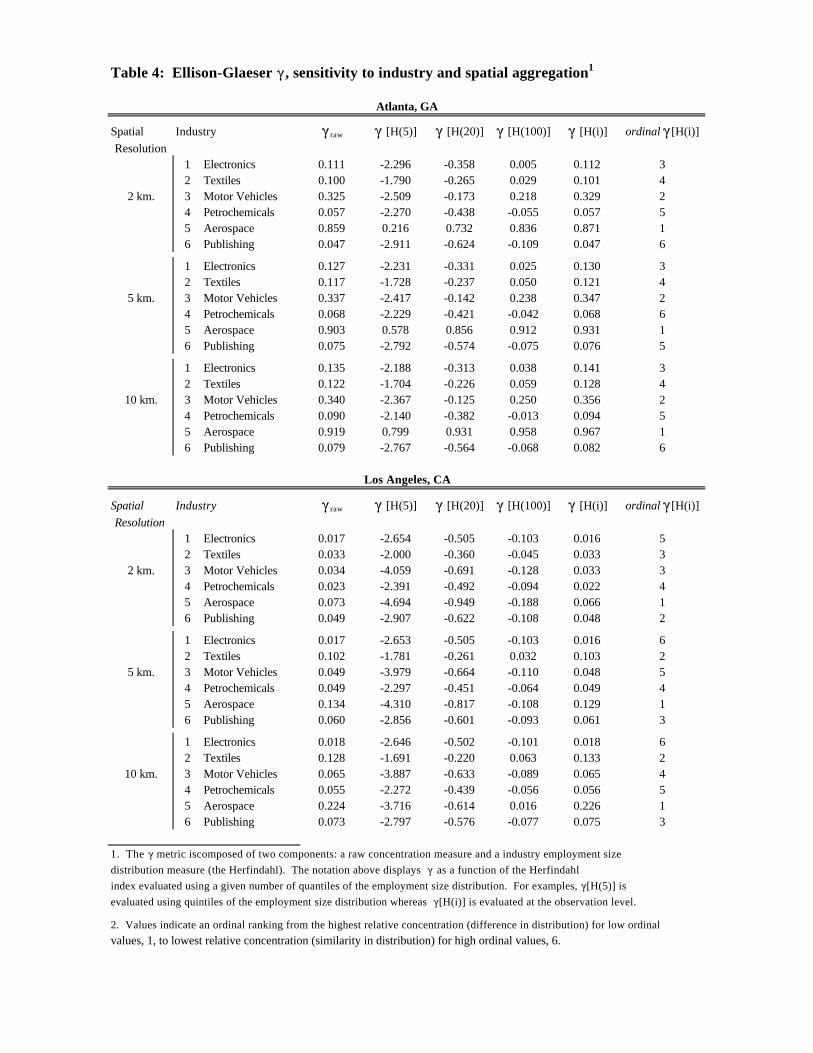
Table 4: Ellison-Glaeser (, sensitivity to industry and spatial aggregation1

Spatial Industry (raw ( [H(5)] ( [H(20)] ( [H(100)] ( [H(i)] ordinal([H(i)]Resolution

1 Electronics 0.111 -2.296 -0.358 0.005 0.112 32 Textiles 0.100 -1.790 -0.265 0.029 0.101 4

2 km. 3 Motor Vehicles 0.325 -2.509 -0.173 0.218 0.329 24 Petrochemicals 0.057 -2.270 -0.438 -0.055 0.057 55 Aerospace 0.859 0.216 0.732 0.836 0.871 16 Publishing 0.047 -2.911 -0.624 -0.109 0.047 6





Spatial Industry (raw ( [H(5)] ( [H(20)] ( [H(100)] ( [H(i)] ordinal([H(i)]Resolution

1 Electronics 0.017 -2.654 -0.505 -0.103 0.016 52 Textiles 0.033 -2.000 -0.360 -0.045 0.033 3

2 km. 3 Motor Vehicles 0.034 -4.059 -0.691 -0.128 0.033 34 Petrochemicals 0.023 -2.391 -0.492 -0.094 0.022 45 Aerospace 0.073 -4.694 -0.949 -0.188 0.066 16 Publishing 0.049 -2.907 -0.622 -0.108 0.048 2

1 Electronics 0.017 -2.653 -0.505 -0.103 0.016 62 Textiles 0.102 -1.781 -0.261 0.032 0.103 2

5 km. 3 Motor Vehicles 0.049 -3.979 -0.664 -0.110 0.048 54 Petrochemicals 0.049 -2.297 -0.451 -0.064 0.049 45 Aerospace 0.134 -4.310 -0.817 -0.108 0.129 16 Publishing 0.060 -2.856 -0.601 -0.093 0.061 3

1 Electronics 0.018 -2.646 -0.502 -0.101 0.018 62 Textiles 0.128 -1.691 -0.220 0.063 0.133 2

10 km. 3 Motor Vehicles 0.065 -3.887 -0.633 -0.089 0.065 44 Petrochemicals 0.055 -2.272 -0.439 -0.056 0.056 55 Aerospace 0.224 -3.716 -0.614 0.016 0.226 16 Publishing 0.073 -2.797 -0.576 -0.077 0.075 3

1. The ( metric iscomposed of two components: a raw concentration measure and a industry employment size distribution measure (the Herfindahl). The notation above displays ( as a function of the Herfindahlindex evaluated using a given number of quantiles of the employment size distribution. For examples, ([H(5)] isevaluated using quintiles of the employment size distribution whereas ([H(i)] is evaluated at the observation level.

2. Values indicate an ordinal ranking from the highest relative concentration (difference in distribution) for low ordinal values, 1, to lowest relative concentration (similarity in distribution) for high ordinal values, 6.

Atlanta, GA

Los Angeles, CA

Table 5: Rank orderings for Los Angeles

Establishments:

Statistic Spatial

Res.1 clustered (dissimilar) ------------------------------------ dispersed (similar)

Localization 2 aerospace vehicles petrochem publishing electronics textiles5 aerospace vehicles petrochem publishing electronics textiles10 aerospace vehicles petrochem publishing electronics textiles

( 2 - - - - - -5 - - - - - -10 - - - - - -

G(s) 2, s textiles publishing petrochem electronics aerospace vehicles

D(s) s textiles publishing petrochem aerospace vehicles electronics

Employment:

Statistic SpatialRes. clustered (dissimilar) ------------------------------------ dispersed (similar)

Localization 2 petrochem vehicles aerospace publishing electronics textiles5 petrochem vehicles aerospace publishing textiles electronics10 aerospace vehicles petrochem publishing textiles electronics

( 2 aerospace publishing textiles vehicles petrochem electronics5 aerospace textiles publishing petrochem vehicles electronics10 aerospace textiles publishing petrochem petrochem electronics

G(s) 2, s textiles aerospace petrochem publishing vehicles electronics

D(s) s textiles publishing petrochem vehicles electronics aerospace

Note: indicates division between clustering and dispersion

indicates statistical insignificance

1. The spatial resolutions for D(s) and G(s) are over a range of distances,s, though G(s) has a mimimum resolution of 2km given its reliance on a grid.

Industry

Industry

Table 6: Rank orderings for Atlanta

Establishments:

Statistic Spatial

Res.1 clustered (dissimilar) ------------------------------- dispersed (similar)

Localization 2 aerospace vehicles petrochem electronics textiles publishing5 aerospace vehicles petrochem electronics textiles publishing10 aerospace vehicles electronics petrochem textiles publishing

( 2 - - - - - -5 - - - - - -10 - - - - - -

G(s) 2, s publishing electronics textiles petrochem vehicles aerospace

D(s) s publishing petrochem electronics textiles aerospace vehicles

Employment:

Statistic SpatialRes. clustered (dissimilar) ------------------------------- dispersed (similar)

Localization 2 aerospace vehicles textiles petrochem electronics publishing5 aerospace vehicles textiles petrochem electronics publishing10 aerospace vehicles petrochem textiles electronics publishing

( 2 aerospace vehicles electronics textiles petrochem publishing5 aerospace vehicles electronics textiles publishing petrochem10 aerospace vehicles electronics textiles petrochem publishing

G(s) 2, s aerospace vehicles publishing electronics textiles petrochem

D(s) s petrochem electronics publishing textiles vehicles aerospace

Note: indicates division between clustering and dispersion

indicates statistical insignificance

1. The spatial resolutions for D(s) and G(s) are over a range of distances, s, though G(s) has a mimimum resolution of 2km given its reliance on a grid.

Industry

Industry

Business location and spatial externalities: Tying ...sweeney/Sweeney_Feser_SISS_chapter.pdfBusiness...

Documents

Transcript of Business location and spatial externalities: Tying ...sweeney/Sweeney_Feser_SISS_chapter.pdfBusiness...