BUSINESS INVESTMENT: RECENT PERFORMANCE AND … · INTRODUCTION The second half of the 1980s...

OECD Economic Studies No . 16. Spring 199 1

BUSINESS INVESTMENT: RECENT PERFORMANCE AND

SOME IMPLICATIONS FOR POLICY

Robert Ford and Pierre Poret

CONTENTS

Introduction . . . . . . . . . . . . . . . . . . . . . . . . . . . . . . . . . . . . . . . . 80

I . The evolution of business fixed investment . . . . . . . . . . . . . . . . 80

II . The determinants of investment . . . . . . . . . . . . . . . . . . . . . . . 87

of investment demand . . . . . . . . . . . . . . . . . . . . . . . . . . . 88 B . Empirical evidence . . . . . . . . . . . . . . . . . . . . . . . . . . . . . 89 C . "Non-neoclassical" explanations . . . . . . . . . . . . . . . . . . . . 101 D . Conclusions on investment demand . . . . . . . . . . . . . . . . . . 108

A . A summary of the "neo-classical" theory

Ill . Public policy and investment . . . . . . . . . . . . . . . . . . . . . . . . . . 109 A . Econometric studies . . . . . . . . . . . . . . . . . . . . . . . . . . . . 109 B . Applied general equilibrium (AGE) models . . . . . . . . . . . . . . 110

IV . The benefits of investment . . . . . . . . . . . . . . . . . . . . . . . . . . . 112 A . Capital formation . . . . . . . . . . . . . . . . . . . . . . . . . . . . . . 112 B . Embodiment effects . . . . . . . . . . . . . . . . . . . . . . . . . . . . 114

V . Conclusions . . . . . . . . . . . . . . . . . . . . . . . . . . . . . . . . . . . . . 116

Annex: Statistical tests on output. capital. the cost of capital and profits . . . . . . . . . . . . . . . . . . . . . . . . . . . . 122

Bibliography . . . . . . . . . . . . . . . . . . . . . . . . . . . . . . . . . . . . . . . . 127

Robert Ford is a Principal Administrator in Country Studies 111 Division. and Pierre Poret is an Administrator in the General Economics Division of the Economics and Statistics Department . The authors are grateful to Andrew Dean. FranCois Delorme. Richard Herd. Peter Hoeller. Constantino Lluch. John P . Martin. Giuseppe Nicoletti. Jeffrey Shafer and Peter Sturm for comments and to Mark Keese and lsabelle Wanner for research assistance .

79

INTRODUCTION

The second half of the 1980s witnessed a major and widespread recovery in business investment expenditures in the OECD countries. Real gross fixed investment by the business sector grew by only 3.8 per cent per year from 1970 to 1979 and stagnated during the recessionary period of 1980 to 1983. In the five years 1984 to 1988 it then grew by almost 7 per cent a year. Nevertheless, the increase in the stock of productive capital - gross investment less scrapped capital - as a proportion of output tailed off in the 1980s in most OECD countries.

These events raise several related questions: what accounts for the recent strength in investment? Can it be expected to continue? Is the deceleration of capital-output ratios a cause for concern? If so, should governments attempt to raise investment? This paper attempts to provide answers, sometimes tentative, to some of these questions. The neo-classical model of investment is used as a framework of analysis, and emphasis is placed on the supply-side aspects of capital formation rather than its business-cycle, or demand-side aspects. The focus is therefore on aggregate business-sector fixed investment, as the bulk of productive capital in OECD economies is in the business sector, and other categories of investment - residential construction, stockbuilding and public sector investment - are not driven by the same economic factors.

Section I assesses the evolution of investment and capital formation in OECD countries over the past two decades. The determinants of investment demand' are analysed in Section II. Section 111 reviews investment policies and their economic effects, concentrating on the U.S. experience with investment incentives during the 1980s. Section IV considers some economic consequences of investment. The final section presents the conclusions.

I. THE EVOLUTION OF BUSINESS FIXED INVESTMENT

Summary statistics of investment performance over the past two decades are provided in Table 1. To account for the influence of the downturn experienced

80

by most OECD economies in 198 1, averages are presented for three sub-periods: 1970-79, 1980-83 and 1984-88. Growth in gross investment expenditures fell sharply in the early 1980s in most countries, but then picked up again and has been higher in the last five years than in the 1970s in most OECD countries.

It is useful to distinguish between gross and net investment when analysing the evolution of the investment-output ratio over time2. The former represents

Table 1. Business fixed investment in the OECD countries: statistical summary

Annual average growth rates ~ ~

Gross business fixed investment

1970-79 1980-83 1984-81

OECD Big 7

United States Japan Germany France Italy United Kingdom Canada

Australia Austria Be I g i u rn Denmark Finland Greece Iceland Ireland Luxembourg Netherlands New Zealand Norway Portugal Spain Sweden Switzerland Turkey

3.9 -0.3 3.8 -0.4

4.0 -1.8 4.3 3.5 3.1 0.1 2.6 -0.6

2.4 -0.6 6.6 2.8

2.6 3.6

1.8 0.1 2.8 -0.9 2.4 7.1

10.3 0.8

1.1 0.6

3.0 9.7 6.6 4.4 3.8 4.1

2.3 1.7 1.9 4.2 9.2 0.5

3.0 -2.7

5.5 -2.3

4.9 -2.9

6.8 -2.4

2.3 -3.5

4.1 -2.3

6.8 6.9

6.7 8.9 4.4 4.4 6.4 8.7 9.0

6.1 5.8 6.6 7.0 4.7 -1.2

7.4 -1.8

9.5 8.0 3.0 5.2 3.6 8.0 7.1 9.1 5.1

Real gross domestic product

970-79 1980-83 1984-81

3.5 3.5

2.8 5.3 3.1 3.7 3.9 2.3 4.7

3.5 4.0 3.5 2.5 3.8 5.4 6.7 4.6 2.7 3.4 1.9 4.5 5.3 3.8 2.5 1.6 5.6

1.3 1.3

0.7 3.6 0.6 1.5 1.7 0.4 1.3

1.5 1.4 1.3 1.1 3.4 0.7 2.0 2.1 1.1 0.1 2.0 2.5 2.0 1 .o 1.1 1.5 3.1

3.8 3.9

4.2 4.5 2.6 2.2 3.0 3.6 4.7

4.5 2.2 2.2 2.3 3.5 2.1 4.4 3.0 4.1 2.4 1.8 3.9 2.8 3.6 2.7 2.7 6.0

As a per cent of business sector value added’ ~ ~

Gross business fixed investment

970-79 1980-83 1984-8f

16.6 16.3 16.7 16.4 16.2 16.7

13.7 14.3 14.7 23.4 21.8 23.6 15.5 15.3 15.6 18.2 16.0 15.5 17.8 15.3 14.9 16.3 15.8 17.2 15.3 19.2 18.1

19.5 21.2 20.5 21.7 19.6 19.9 14.7 13.8 14.5 17.4 14.9 18.8 21.2 19.1 19.4 15.6 14.5 11.4 23.1 21.0 20.5 21.6 23.1 15.8 20.3 19.3 18.0 17.0 13.9 16.1 22.2 23.8 26.2 27.5 23.4 22.6 24.6 23.6 19.1 17.2 15.5 14.9 16.6 15.9 18.0 14.4 15.6 18.8 15.4 12.0 11.8

Net business fixed investment

970-79 1980-83 1984-88

10.2 8.6 8.4 9.8 8.5 8.3

7.2 6.8 6.6 15.4 12.8 13.4 10.1 8.1 7.7 11.4 7.7 6.2 11.1 8.2 7.7 9.5 6.6 6.9

11.3 14.6 12.9

12.8 12.7 11.3 14.0 10.0 8.9 9.6 7.6 7.2

13.0 8.7 11.9 13.3 9.6 9.6 13.7 11.7 7.6 19.2 16.8 15.5 16.0 17.2 9.0 15.1 13.9 12.0 9.6 4.7 5.9

14.7 13.9 15.3 18.1 13.6 14.0 17.3 13.4 6.2 13.6 10.5 8.4 10.2 8.3 10.4 9.5 8.6 11.0

12.2 8.4 7.8

1. Businesssector value added is defined as GDP at factor cost less the deflated government sector wage bill and (where available) government sector capital cost allowance.

81

demand for output and is important for business cycle analysis because of its cyclical volatility relative to most other components of aggregate demand. Net investment, on the other hand, is the addition to the productive capital stock and is relevant to the analysis of aggregate supply and productivity.

Chart 1 compares gross and net investment-output ratios for the OECD countries. Gross ratios have been roughly stable or have risen in most countries over the past three decades. However, net investment-output ratios have not kept pace and have even fallen in many countries. The investment boom of the late 1 980s boosted net investment-output ratios, although they have generally not returned to levels seen in the 1960s and 1970s and, for the OECD as a whole, were no higher in the 1984-88 period than during the recession. As a result of the decline in net investment ratios, capital-output ratios tended to fall below trends set in the 1960s and 1970s (Ford and Poret, 1990). The widening gap between gross and net investment-output ratios is at least in part due to increases in scrapping rates3. This has occurred both because the mix of the capital stock has shifted to shorter-lived types of capital (such as machinery, as opposed to structures) and because of an increase in the rate of scrapping of particular types of capital. The latter effect has been associated with the rapid introduction of computerised equipment in the last couple of decades. However, given the lags and imprecision associated with estimates of service lives, the accelerated scrapping associated with computerisation has probably not been adequately captured in the data presented here. Thus, the gap has probably grown more than Chart 1 would suggest.

Although most OECD economies have had similar patterns of investment over time, levels of investment in relation to output vary widely from country to country. In terms of gross investment, the United States, Italy, Belgium, Greece, Spain and Turkey were a t the bottom end, averaging less than 15 per cent of business output between 1984 and 1989. Japan, Australia, Iceland, New Zealand and Norway were a t the top end, with more than 20 per cent. In terms of net investment, the United States, France, the United Kingdom, the Netherlands and Portugal were a t the lower end, with investment being less than 7 per cent of business output, and Japan, Iceland, New Zealand and Norway were at the upper end at over 13 per cent4.

This picture of the evolution of capital formation may be distorted due to the omission or significant under-measurement of important components of the capital stock. Two such components that have recently drawn considerable attention are computers and so-called intangible capital.

In the case of computers, the major issue has been the proper measurement of the "real" quantity of computers or, equivalently, the price of a typical computer. Advances in electronic technology, from vacuum tubes to transistors to integrated circuits, have resulted in dramatic declines in the price of carrying out a

02

CHART 1

BUSINESS SECTOR GROSS AND NET INVESTMENT/OUTPUT RATIOS

United Kingdom

- 34 - 32 - 30 - 28 - -

- 26 - - 24 -

22 - 20 -

-

-

-Gross investment/output (left scale) ----- Net investment/output (right scale)

Per cent United States Per cent Per cent France Per cent

24

22

20

18

16

14

Japan

Germany

24 34 32

22 30 20 28 18 26

16 24 22

l4 20

10 16

6 10

12 18

14 12

4 8

- 24 - 22 - 20 - 18 - 16 - 14 - 12 - 10 - 8

- 6

- 4

Italy

60’62 64 66 68 70 72 74 76 78 80 82 84 86 88 60 62 64 66 68 70 72 74 76 78 80 82 84 86 88

83

CHART 1 (continued)


-Gross investrnent/output (left scale] ----- Net investrnent/output (right scale)

- 34 - 32 - 30 - 28 - - 26 - 24 -

-

- -

8%

Per cent Canada Per cent

24

22

20

18

16

Austria

Belgium

24

22

20

18 i 16

f 4

Per cent Denmark Per cent

Finland

24

22

20

18

Greece

30 28 26 24 c I

8- 60 62 64 66 68 70 72 74 76 78 80 82 84 86 88

16

14

12

10

8

6

4 60 62 64 66 68 70 72 74 76 78 80 82 84 86 88

84

CHART 1 (continued)


- Gross investment/output (left scale] -.---Net investment/output (right scale]

Per cent Iceland Per cent Per cent Spain Per cent

Netherlands

I Norway I

10 :: 8 60 62 64 66 68 70 72 74 76 78 80 82 84 86 88

34 - 32 - 30 28 - -

26 - 24 - 22 - 20 - 18 - 16 - 14 - 12 10 -

- 8 -

34 - 32 - 30 - 28 - 26 24 -

- 22 20 18 16 14 12

- - - - -

10 - -

8 -

Sweden

Switzerland

24 34 - 24 - 32 -

- 22 22 30 - ' 20 28 - - 20

18 26 - 18 - 16 24 - 16

- 22 -

12 18 12 .----a-.-----

10 16 10

6 10 - 4 8 ~ I I I I I I I I I ~ I I I I I I I I I I I I I I I I I I ~ 4

; - - - 8

- 6

14 \r ---,. ----.-/ - 12 -

60 62 64 66 68 70 72 74 76 78 80 82 84 86 88

85

Per cent

26 24 22

14 12 10 8

CHART 1 (continued1

- - - 8

- 6

- 14 - - 1 2 -

-

- - 6 1 0 - ~ l l l l l l l l l l l l l l l l l l l l I I I I I I I h 4 8 ~ ~ I I I I I I I I I I I I I I I I I I I I I I I I I I c , 4


- Grass investrnent/autput (left scale) ----- Net investrnent/autput (right scale]

Australia Per cent Per cent New Zealand Per cent

j :: i; [ 20

typical computation. Berndt and Griliches ( 1990), using hedonic price indices, found that the nominal quality-adjusted price of PCs fell by about 25 per cent per annum in the United States from 1982-88. Gordon (19891, using a matched- model procedure, found nominal price declines of almost 24 per cent per annum from 1 982-875. For comparison, the U.S. consumer price index rose, on average, by about 3.2 per cent per annum from 1982-88.

However, conventional national accounting practices do not take full account of the improvement in computing power and it is now widely believed that they overstate the price and, given nominal expenditures, understate the real quantity of computer investment. One solution, pioneered by the U.S. Bureau of Economic Analysis (BEA) and since adopted by Canada and Australia, is to adjust explicitly for quality changes using a hedonic price index6. Several other countries - Japan, France, Denmark and Sweden, for example - are likely to make similar adjustments.

A crude estimate of the effect of proper quality adjustment can be obtained by applying the BEA deflator to nominal computer expenditures in other OECD countries to adjust the "real" shares of computers in total business fixed invest- ment7. Typically, the adjusted share is higher by 2 to 4 percentage points by 1987, and the effect grows over time, along with the share of computers in investment.

86

The issue with regard to intangible investment is the somewhat arbitrary, from an economic viewpoint, national-accounts definition of capital. Capital, as currently defined in the national accounts, must be tangible, durable (i.e. have a service life exceeding one year), fixed (inventories and goods-in-process are not included) and produced (natural forests, land and mineral deposits are not included). Many expenditures, such as research and development (R&D), computer software, marketing and training and education, are similar to traditional investments in that they add to long-term productive potential. However, as there is no physical "stock", these intangibles are currently treated in national accounts as intermediate inputs, not investment (although a number of categories of expenditures on intangibles are likely to be reclassified in the next round of revisions to national accounting methodology) (Blades, 1 989).

Studies of the Finnish industrial sector (Tilastokeskus, 1989) and the Swedish manufacturing sector (Koll and Nockhammar, 1989) found that intangible investment accounted for about 28 and 53 per cent of total investment (including intangibles) in Finland and Sweden, respectively. Both studies also found that R&D accounted for roughly half of all intangible investment. To illus- trate the consequences of putting R&D on the same footing as conventional investment, figures on real R&D expenditures, assembled by the OECD Director- ate for Science, Technology and Industry, were added to national accounts business investment. According to these data, the ratio of business R&D to business investment expenditure (i.e. under the current national accounts definitions) was almost 1 1 per cent in the OECD as a whole over the last two decades, and it increased by almost 3 percentage points from the 1970s to the 1980s. Had R&D been included in business fixed investment, the OECD average gross investment-output ratio would have been about 2 percentage points higher in the late 1980s.

II. THE DETERMINANTS OF INVESTMENT

The broad developments in aggregate business fixed investment expendi-

the recovery in output growth after the 1981-82 recession raised the demand for capital and, hence, investment; rates of return to capital recovered to pre-recession levels; the cash flow and leverage positions of firms improved; the cost of equity finance fell as stock markets boomed;

tures in the 1980s might be explained as follows: -

- - -

87

- although conditions varied from country to country, on balance the economic climate was less volatile during the extended boom of the 1980s than in the 1970s; and the introduction of new innovations, particularly in computer technology, ought to have raised the marginal productivity of capital.

At the same time, significantly higher real interest rates, wage moderation in most OECD countries and the winding down of investment incentives may have reduced the demand for capital: firms shifted to somewhat less capital-intensive production techniques.

This explanation is broadly consistent with standard theories of investment demand. However, it must be tempered by the fact that investment behaviour is poorly understood at the empirical level, a case that will be argued more fully below. One manifestation of this is that investment demand equations have proved to be among the most difficult of all macroeconomic relationships to estimate reliably. As a result, even after decades of research there remains significant disagreement about the importance for investment demand of interest rates, investment incentives and even output.

-

A. A summary of the "neo-classical" theory of investment demand

According to standard "neo-classical" theory, as described, for example, by Kopke (1 985). Chirinko ( 1986) or Catinat et al. ( 19871, firms choose output and factor inputs so as to maximise profits. Assuming the production function has constant elasticity of substitution, the demand for capital can be specified in terms of output and the real cost of capital. In the neo-classical interpretation, the level of output is chosen by the firm and the real cost of capital determines the capital intensity of production. An alternative, "Keynesian", interpretation of the output term is that the firm is sales-constrained8. This article stresses the neo- classical interpretation, which implies that the coefficient on the cost of capital is a measure of the elasticity of substitution, but also that part of the cost of capital effect on investment demand is buried in the output term.

It is generally assumed that various costs delay the adjustment of the actual stock of capital employed by firms to the level implied by the profit-maximisation conditions. These adjustment costs are crucial to the theory, because if there were no such costs profit-maximising firms would simply install all desired capital immediately and there would be no well-defined demand for investment. These costs also explain why a competitive firm has a determinate desired output, even with a constant returns-to-scale production function: with adjustment costs, capital is a quasi-fixed factor.

The cost of capital is made up of several components: the real purchase price of investment goods; the cost of financing the purchase of a piece of capital; the

88

depreciation rate; the tax rate on corporate income; the expected present value of depreciation allowances; and investment tax credits

g. Government policy alters

the demand for capital and, therefore, investment by influencing interest rates or by changing the fiscal regime faced by firms. The key parameter determining the leverage exerted by policy is the elasticity of substitution between capital and the other factor inputs, which summarises the effect of a change in the cost of capital on the demand for capital. If it is zero, the cost of capital is irrelevant to the firm's investment decision, given its choice of output, yielding the special case of the pure accelerator model.

B. Empirical evidence

1. A brief review of investment demand estimation

The determinants of investment demand can be conveniently (if somewhat artificially, particularly under the neo-classical interpretation) broken down into two parts: the accelerator, which captures the relationship between output and capital as determined by a production function, and the cost of capital effect, which captures the substitutability between capital and other factors of production. There is broad consensus that the former is a robust relationship, based on the close correlation between the growth rates of business fixed investment and output at an annual frequency, as shown in Chart 2 ' O . This correlation poses a difficulty, however, since the accelerator predicts that the growth rate of the capital stock (that is, the first, rather than the second, difference of the log of the capital stock) ought to be correlated with output growth. Nevertheless, adjustment costs can be invoked to explain the observed correlation: the acceleration in investment may be prolonged if a shock to output growth is accompanied by a slow adjustment of the capital stock. This issue is analysed a t length below.

Gordon and Veitch (1987) provided a dissenting view on the accelerator, arguing that investment is best explained by its own lags. This possibility is examined in detail below. Bennett ( 1 989) argued that the firm determines both output and investment at the same time and that therefore the ordinary least squares estimate of the accelerator will be biased upwards. He used fiscal policy variables as instruments to control for simultaneity bias and found that the importance of output in the determination of investment is reduced.

Although the accelerator affect is widely accepted, there is considerable controversy about the role of the cost of capital. While most economists believe it has a small effect on investment demand, others (Clark, 1979; Blanchard, 1986; and Gordon and Veitch, 1987, for example) have concluded that there is little or no empirical evidence that the cost of capital affects investment demand. Indeed, a robust empirical relationship between the cost of capital and investment has proved very elusive.

89

CHART 2

OUTPUT GROWTH AND CHANGE IN THE GROWTH OF THE CAPITAL STOCK

- - -

- - - - -

-Real business gross fixed capital stock (left scale) ----- Real gross domestic product (right scale)

Per cent United States Per cent Per cent France Per cent

- 7

- 6

- 5

- 4

- 3

- 2

- 1

- 0

0.8 r

- - -

- 1

- 6

- 5

- 4

- 3

- 2

- 1

- 0

-1

-2

-3

0.8

0.6

0.4

0.2

0

-0 .2

-0.4

4.6

4.8

-1 .o -1.1

1 Japan I 0.8

0.6

0.4

0.2

0

4 . 2 4 . 4

4 . 6

4 . 8

-1 .o -1.2

Germany 0.8 c 0.6

0.4

0.2

0

4 . 2

4 . 4

4.6

4 . 8

-1 .o -1.2

-1.4

9

8

1

6

5

4

3

2

1

0

-1

-2

t 1 Italy

0.6

0.4

0.2

0

4 . 2

-0.4

4 . 6

4 . 8

1 United Kingdom L 8

1

6

5

4

3

2

1

0

-1

-2

-3 60 62 64 66 68 70 72 74 76 78 80 82 84 86 88 60 62 64 66 68 70 72 74 76 78 80 82 84 86 88

90

CHART 2 (continued)


--Real business gross fixed capital stock (left scale] -----Real gross domestic product (right scale]

Per cent Canada Per cent Per cent Denmark Per cent

0.8

0.4

0 -

-0.4

4 . 8

-1.2

-1.6

1.0

0.8 0.6

0.4

0.2

0 - 0 . 2

-0.4

- 0.6

- 0 . 8

-1.0

-1.2

- - - -

-

- - -

- - - -

I Austria

1

1.0 r 1

Finland

1.0 c - - 9

- 6 0.8 -

- 0 -1.0 - 1

-1.2 - 0

- -

Belgium Greece - 7 2.0 - - - 10

- 8

-

- 1 -1.0 -

- 0 -1.5 - - - -1 -2.0 - -2 -

-0.6 -2 -2.5 1 1 1 1 1 1 1 1 1 1 1 1 1 J 1 " l " l l l l l l l ' l O I I I I I I 1 l I I I 60 62 64 66 68 70 72 74 76 78 80 82 84 86 88 60 62 64 66 68 70 72 74 76 78 80 82 84 86 88

91

CHART 2 (continued)


-Real business gross fixed capital stock (left scale) ..--- Real gross domestic product (right scale)

Per cent

7 12 Spain Per cent

I-

Per cent Ireland Per cent

- 8

3 - 0.4 -

- -1.2 -

- - -1

Netherlands 0.8 1 8

0.6 . 0.4 .

0.2 '

0 '

- 0.2 '

-0.4 .

-0.6 . -0.8 .

-1.0 .

1.2 c Norway

1 -2

- 1 7

0.8

0.4

0

-0.4

-0.8

-1.2

-1 6

0.8 L - 1 7 Sweden

I Switzerland I 0.6 - 0.4 - \ 0.2

/? # '

- 0 -

- 0 . 2 - -0.4 - - 0.6 -

-0.8

-1.0 - -

- -2

-4

- 4

60 62 64 66 68 70 72 74 76 78 80 82 84 86 88

92

expectations. Compounding these problems is the fact that different firms may face different tax rates. Using panel data, Devereux (19891, for the United Kingdom, and Anderson (19881, for Canada, found that taxation had a large influence on the investment behaviour of firms that had not exhausted their tax expenditures.

Finally, it has been argued that different types of investment should not be aggregated. Norotte and Bensaid ( 1 987) and Evans ( 1 989) have suggested that the unusually rapid growth of computer investment poses a problem for econometric estimation of aggregate investment equations. By excluding computers, both studies were able to find stable investment demand functions, for France and the United States, respectively.

An elegant solution to many of the difficulties faced by the standard imple- mentation of neo-classical investment demand functions is Tobin's Q modeV3. Tobin's Q is defined as the ratio of the market value of an additional unit of capital to its replacement cost. As the market value is just the expected present value future returns from the piece of capital, the firm can increase its profits (or its market value) by investing when Q exceeds unity. The Q model is equivalent to a version of the standard neo-classical investment model (Hayashi, 1982) but, in principle, has the advantage that all relevant information about expectations is summarised in the Q ratio itself. That is, the market's judgement of the future stream of net earnings ought to be reflected in the market value of the firm. Thus, to the extent the "market" is correct in its assessment, there is no need to measure expectations directly.

Unfortunately, Q models have not enjoyed a great deal of empirical success. Chirinko (1986) provides a brief survey of results from the United States and a discussion of the drawbacks of Q. The empirical weakness of Q is not due to factors specific to the U.S. economy: Poret and Torres (1987) and Mullins and Wadhwani ( 1989) document the relatively poor performance of Q for several other countries.

Measurement errors are the most common reason advanced for the disappointing performance of Q. First, the theory specifies marginal 0, but only average Q is observable and the two may diverge. Abel and Blanchard (1986) constructed a series for marginal Q for the United States, but the results were not improved. Second, the variation in the market value of the firm, the numerator of 0, is dominated by the value of equity which may be excessively volatile in that its movements may not reflect only changes in expected future profits (Shiller, 1981). However, Barro (1989a) found stock prices, but not Q, to be an important factor explaining investment in the United States, and Mullins and Wadhwani ( 1 989) found that stock market variables were statistically significant in the United States and the United Kingdom, although not in Japan or Germany. If there is a measurement problem, these results suggest it may lie in components of Q other than stock prices. Finally, Schaller ( 1 990) has argued that firm-specific

94

effects contaminate aggregated time series investment data, and that better estimates can be obtained from firm-level data.

2. Estimates of investment demand functions for the seven largest OECD economies

The previous sub-section surveyed only a small part of the vast literature on investment demand. The thrust of most of this work has been to attempt to improve either the data used in estimation or the specification of the demand functions. However, the major puzzles remain largely unresolved. To help shed light on these, the statistical properties of capital, output and cost of capital data are examinedq4. This is followed by a regression analysis of the same data. The analysis is restricted to data for the seven largest OECD economies.

Three types of statistical tests were carried out:

i) unit root tests to determine the order of integration of these variable^'^; ii) cointegration tests to determine if there is a long-run relationship

between them16; and iii) causality tests to investigate further the appropriate specification of the

factor demand f~nctions'~. The details of these tests are described in the Annex. In summary, they

reveal the following picture'*. Output and the cost of capital are integrated of order 1 (written I( 1 )). In the

case of capital the results are difficult to interpret. According to the unit root tests, capital is 1(2), implying that output and the capital stock cannot be cointegrated. However, gross investment is 1(1), and the method by which the capital stock is constructed suggests that it should have the same order of integration as gross investment. Thus, capital may be either l(1) or l(2).

In any case, output, capital and the cost of capital are not cointegrated, casting doubt on the standard view that net investment is a process of adjustment of the capital stock to a "desired" level linked to output and the cost of capital by a stable production function.

The causality tests suggest that lagged output does not "cause" investment, nor does lagged investment "cause" output, at least for most countries. Unfortunately, these tests shed no light on the difficult issue of possible simultaneity between contemporaneous output and investment.

The cointegration results imply that regressions on the levels of the variables are unlikely to be sensible. However, regressions on their first differences, as long as they are stationary, may yield consistent estimates. Since the order of integration of the capital stock cannot be ascertained with confidence, two variants of the neo-classical investment function were specified. The first, reported in Tables 2a and 2b, regresses the growth rate of the capital stock against its own lags, output growth and the growth rate of the cost of capital, assuming capital to

95

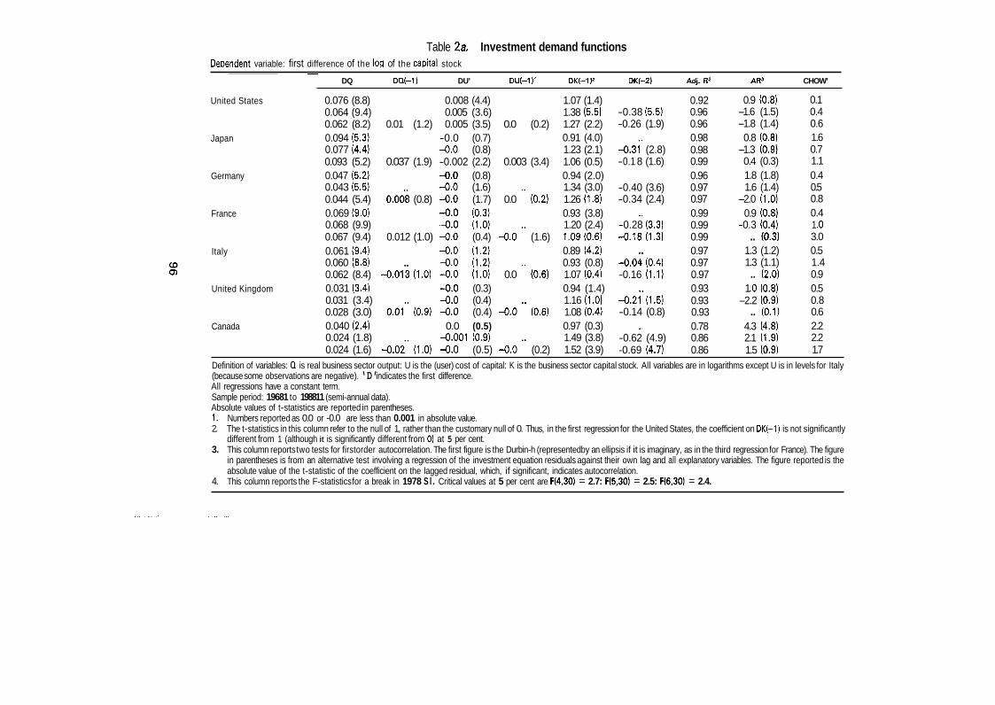
Table 2a. Investment demand functions DeDendent variable: first difference of the 1011 of the caDital stock

~

DQ DQ(-l) DU’ DU(-l)’ DK(-1l2 DK(-2) Adj. R2 AR’ CHOW’

United States 0.076 (8.8) 0.008 (4.4) 1.07 (1.4) 0.064 (9.4) 0.005 (3.6) 1.38 (5.5) 0.062 (8.2) 0.01 (1.2) 0.005 (3.5) 0.0 (0.2) 1.27 (2.2)

0.91 (4.0) 0.077 (4.4) -0.0 (0.8) 1.23 (2.1) 0.093 (5.2) 0.037 (1.9) -0.002 (2.2) 0.003 (3.4) 1.06 (0.5)

Germany 0.047 (5.2) -0.0 (0.8) 0.94 (2.0) 0.043 (5.5) -0.0 (1.6) 1.34 (3.0) 0.044 (5.4) 0.008 (0.8) -0.0 (1.7) 0.0 ’’ (0.2) 1.26 (1.8)

France 0.069 (9.0) -0.0 (0.3) 0.93 (3.8) 0.068 (9.9) ,4.0 (1.0) 1.20 (2.4) 0.067 (9.4) 0.012 (1.0) -0.0 (0.4) -0.0 ’ * (1.6) 1.09 (0.6)

-0.0 (1.2) 0.89 (4.2) 0.060 (8.8) -0.0 (1.2) 0.93 (0.8) 0.062 (8.4) -0.013 (1.0) -0.0 (1.0) 0.0 ’’ (0.6) 1.07 (0.4)

United Kingdom 0.031 (3.4) -0.0 (0.3) 0.94 (1.4) 0.031 (3.4) -0.0 (0.4) 1.16 (1.0) 0.028 (3.0) 0.01” (0.9) -0.0 (0.4) -0.0 ‘ * (0.6) 1.08 (0.4)

Canada 0.040 (2.4) 0.0 (0.5) 0.97 (0.3) 0.024 (1.8) -0.001 (0.9) 1.49 (3.8) 0.024 (1.6) -0.02‘ (1.0) -0.0 (0.5) -0.0 ’ * (0.2) 1.52 (3.9)

Japan 0.094 (5.3) -0.0 (0.7)

Italy 0.061 (9.4)

-0.38 (5.5) -0.26 (1.9)

-0.3i’ (2.8) -0.1 8 (1.6)

-0.40 (3.6) -0.34 (2.4)

-0.28 (3.3) -0.18 (1.3)

-0.04 (0.4) -0.16 (1.1)

-0.2i’ (1.5) -0.14 (0.8)

-0.62 (4.9) -0.69 (4.7)

0.92 0.96 0.96 0.98 0.98 0.99 0.96 0.97 0.97 0.99 0.99 0.99 0.97 0.97 0.97 0.93 0.93 0.93 0.78 0.86 0.86

0.9 (0.8) -1.6 (1.5) -1.8 (1.4)

0.8 (0.8)

0.4 (0.3) 1.8 (1.8) 1.6 (1.4)

-2.0 (1 .O) 0.9 (0.8)

-0.3 (0.4) .. (0.3)

1.3 (1.2) 1.3 (1.1) .. (2.0)

1 .O (0.8) -2.2 (0.9)

.. (0.1) 4.3 (4.8) 2.1 (1.9) 1.5 (0.9)

-1.3 (0.9)

0.1 0.4 0.6 1.6 0.7 1.1 0.4 0.5 0.8 0.4 1 .o 3.0 0.5 1.4 0.9 0.5 0.8 0.6 2.2 2.2 1.7

Definition of variables: 0 is real business sector output: U is the (user) cost of capital: K is the business sector capital stock. All variables are in logarithms except U is in levels for Italy (because some observations are negative). ‘D’ indicates the first difference. All regressions have a constant term. Sample period: 19681 to 198811 (semi-annual data). Absolute values of t-statistics are reported in parentheses. 1. Numbers reported as 0.0 or -0.0 are less than 0.001 in absolute value. 2. The t-statistics in this column refer to the null of 1, rather than the customary null of 0. Thus, in the first regression for the United States, the coefficient on DK(-1) is not significantly

different from 1 (although it is significantly different from 0) at 5 per cent. 3. This column reports two tests for firstorder autocorrelation. The first figure is the Durbin-h (represented by an ellipsis if it is imaginary, as in the third regression for France). The figure

in parentheses is from an alternative test involving a regression of the investment equation residuals against their own lag and all explanatory variables. The figure reported is the absolute value of the t-statistic of the coefficient on the lagged residual, which, if significant, indicates autocorrelation.

4. This column reports the F-statistics for a break in 1978 S l . Critical values at 5 per cent are F(4,30) = 2.7: F(5,30) = 2.5: F(6,30) = 2.4.

Table 2b. Investment demand functions Dependent variable: first difference of the log of the capital stock

United States

Japan

Germany

France 0 w

Italy

United Kingdom

Canada

D W l ) DU(-1)' DK(-l)* DK(-2) DKl-3) Adj. R2 AR3 ch0w4

0.06 (6.1) 0.02 (1.2) 0.01 (0.6)

0.09 (4.0) 0.07 (3.01 0.07 (3.0)

0.02 (2.1) 0.004 (0.3) 0.01 (1.0)

0.02 (1.4) -0.02 (1.0) -0.03 (1.1)

0.02 (1.3) 0.00 (0.0) 0.001 (0.0)

0.02 (2.1) 0.02 (1.6) 0.02 (1.6)

0.03 (1.9) -0.01 (0.8) -0.01 (0.9)

-0.002 (0.7) -0.004 (1 -6) -0.005 (1 -8)

0.0 (0.1) 0.0 (0.21 0.0 (0.3)

-0.0 (0.8) -0.0 (0.5) -0.0 (1.4)

-0.01 (1.7) -0.01 (1.7) -0.01 (1.5)

-0.0 (1.8) -0.0 (1.6) -0.0 (1.5)

-0.0 (0.8) -0.0 (0.8) -0.0 (0.8)

-0.003 (1.4) -0.001 (1.0) -0.001 (0.6)

0.93 (1.1) 1.35 (1.7) 1.56 (1.9)

0.90 (4.2) 1.12 (0.7) 1 .I 6 (0.9) 0.94 (1.5) 1.40 (2.2) 1.1 6 (0.8)

0.96 (1.2) 1.58 (2.2) 1.66 (2.1)

0.89 (2.2) 1.1 5 (0.5) 1.16 (0.6)

0.93 (1.7) 1 .oo (0.1 ) 1 .oo (0.1 ) 0.96(0.5) 1.49 (3.4) 1.58 (3.6)

-0.49 (2.1 1 -0.85 (2.0)

-0.21 (1.4) -0.31 (1.2)

-0.44 (2.4) 0.1 4 (0.5)

-0.59 (2.4) -0.77 (2.0)

0.24 (0.9) 0.35 (1.1)

-0.08 (0.4) -0.11 (0.4)

-0.71 (4.9) -0.93 (3.3)

0.85 0.87

0.17 (1.0) 0.87

0.98 0.98

0.07 (0.5) 0.98

0.95 0.95

-0.36 (2.5) 0.96

0.96 0.96

0.11 (0.6) 0.96

0.91 0.91

0.10 (0.7) 0.91

0.92 0.92

0.02 (0.1 ) 0.92

0.76 0.86

0.1 5 (0.9) 0.85

-0.11 (0.1) 0.4 .. (0.3) 1 .o .. (0.5) 1 .o

-0.2 (0.03) 1.1 .. (0.6) 0.5 .. (0.9) 0.5

1.0 (1.2) 0.1 .. (2.8) 0:6 .. (0.8) 0.4

0.75 (1 -2) 1.8 .. (0.6) 1.9 .. (1.0) 1.5

0.08 (0.04) 0.2 .. (1.61 0.3 .. (2.2) 0.4

0.4 (0.4) 1.2 .. (0.2) 1.1 .. (0.5) 1.4

4.1 (5.2) 2.3 1.3 (0.9) 1.3 .. (0.8) 1.1

See Table 2a for footnotes and other information.

be l(1). The second, reported in Tables 3a and 3b, is similar except the second difference of the log of the capital stock (which is certainly stationary) is used instead of the first difference.

In Tables 2a and 3a, current values of the change in output and the cost of capital are among the explanatory variables, raising the issue of possible simultaneity bias. According to neo-classical theory, investment and output are determined simultaneously by the firm, as was discussed above. This raises the possibility that the least-squares regression coefficient on contemporaneous output will be biased upwards. Thus, regressions were carried out using only lags of the explanatory variable^'^, and the results are reported in Tables 2b and 36.

Only limited experimentation with specification and variable definitions was carried out. Further lags were not significant (with a few exceptions) and, using different definitions of the variables such as gross investment, investment-capital ratios and output-capital ratios, did not alter the main conclusions. No effort was made to "tune" the equations by including country-specific variables (dummies, for example), adjusting sample lengths and so forth.

Taking the results in Table 2a first, the coefficient on the lagged dependent variable is very high and often insignificantly different from unity. This result reinforces the impression given by the unit root tests that the dependent variable should be differenced again to make it stationary. In the first regression for each country, the coefficient on contemporaneous output growth is positive and significant for all countries, but lagged output growth is always insignificant, except for Japan, where it is marginally significant. The coefficient on the cost of capital is almost always small and insignificant, except for the United States, where it has the wrong sign. Overall, these regressions seem fairly well specified: the R- squared is high, there is little sign of either autocorrelation or a structural break. While they provide support for the accelerator hypothesis, this may be due to simultaneity bias. Moreover, the high coefficient on the lagged dependent variable, along with the unit root tests reported above, suggests that the regressions are actually picking up the correlation between the growth rate of output and the growth rate of investment.

The regressions reported in Table 2b use only lags of output and the cost of capital as regressors. Again, the cost of capital plays little role and the coefficient on the lagged dependent variable is typically close to unity. In the first regression for each country, the coefficient on the lagged growth rate of output is positive and usually at least marginally significant. However, as more lags of the dependent variable are added, the size and significance of the coefficient on output growth tend to fall. In effect, lagged output growth and the lagged dependent variable "compete" and, for most countries, the latter "wins". Thus, the results from Tables 2a and 2b suggest that the accelerator is confined principally to the contemporaneous relationship between investment and output.

98

Table 3a. Investment demand functions Dependent variable: second difference of the log of the capital stock

DQ DQ(-1) DU’ DU(-l)’ D2K(-1) D2K(-2) Adj. R2 ARz CHOWJ

United States

Japan

Germany

France

CO CO

Italy

United Kingdom

Canada

0.065 (1 2.3) 0.061 (9.3) 0.064 (8.9) 0.046 (2.5) 0.078 (3.3) 0.085 (3.5) 0.040 (4.8) 0.040 (4.6) 0.037 (4.0) 0.058 (7.2) 0.055 (6.9) 0.056 (7.3) 0.057 (7.1) 0.062 (7.7) 0.062 (7.4) 0.032 (3.5) 0.030 (3.1 ) 0.030 (3.1) 0.038 (3.3) 0.036 (2.4) 0.032 (0.2)

0.012 (1.1) 0.01 7 (1.5)

-0.020 (0.8) -0.020 (0.8)

-0.001 (0.1) -0.002 (0.2)

4 - 0 2 . (1.7) -0.02 (2.0)

-0.033 (2.8) -0.032 (2.7)

0.009 (0.8) 0.009 (0.8)

-0.003 (0.2)

0.005 (3.7) 0.005 (3.6) 0.005 (3.7) -0.0 (00.5) -0.001 (1.2) -0.0 (0.7) -0.0 (1.5) -0.0 (1.5) -0.0 (1.5) -0.0 (0.4) -0.0 (0.2) -0.0 (0.2) -0.0 (0.9) -0.0 (0.5) -0.0 (0.5) -0.0 (0.3) -0.0 (0.3) -0.0 (0.3) -0.002 (1.4) -0.002 (1.1)

0.38 (5.8) 0.0 (0.2) 0.28 (2.3) 0.0 (0.4) 0.16 (0.9)

0.36 (2.8) 0.003 (2.4) 0.40 (2.9) 0.003 (2.4) 0.49 (3.2)

0.38 (3.2) 0.0 (0.1) 0.39 (2.6) -0.0 (0.3) 0.31 (1.9)

0.24 (2.3) -0.0 (1.3) 0.46 (3.0) -0.0 (0.9) 0.54 (3.4)

0.02 (0.2) 0.0 (0.8) 0.34 (2.3) 0.0 (0.8) 0.34 (2.2)

0.22 (1.5) -0.0 (0.5) 0.15 (0.9) -0.0 (0.5) 0.15 (0.8)

0.56 (4.4) -0.0 (0.4) 0.57 (4.1)

0.10 (1.0)

-0.2 (1.3)

0.15 (1.2)

-0.18 (1.7)

-0.004 (0.4)

0.01 (0.07)

0.86 0.85 0.85 0.32 0.38 0.39 0.47 0.44 0.44 0.60 0.63 0.65 0.56 0.62 0.61 0.23 0.20 0.18 0.43 0.40

-1.6 (1.5) -1.7 (1.4)

.. (0.9) 1.2 (1.4) 3.3 (2.5) 8.4 (2.71

-0.4 (0.3)

.. (0.4) 2.8 12.6) .. (0.2) .. (1.5)

2.9 (2.7) 2.0 (0.7) .. (0.7)

-1.4 (0.7) .. (0.0) .. (0.2)

2.2 (1.6) 2.9 (1.8)

-1.5 (0.4)

0.4 0.7 0.8 4.1 4.5 6.0 1.3 1.5 1.1 4.6 4.9 3.4 5.4 2.1 1.7 1.1 0.9 1 .o 3.4 2.2 1.6 . . -0.005 (0.4) -0.002 (1.3) 0.0 (0.2) 0.74 (4.3) -0.27 (1.6) 0.43 .. (1.3)

Definition of variables: as in Table 2, except D2K denotes the second difference of the log of the capital stock. All regressions have a constant term. Sample period 19681 to 198811 (semi-annual data). Absolute values of t-statistics are reported in parentheses. 1. Numbers reported as 0.0 or -0.0 are less than 0.001 in absolute value. 2. This column reports two tests for first-order autocorrelation. The first figure is the Durbin-h statistic (represented by an ellipsis if imaginary, as in the third regression for the United

States). The figure in parentheses is from an alternative test involving a regression of the investment equation residuals against their own lag and all explanatory variables. The figure reported is the absolute value of the t-statistic of the coefficient of the lagged residual, which, if significant, indicates autocorrelation.

3. This column reports the F-statistics for a break in 19781. Critical values at 5 per cent are F(4,301 = 2.7, F(5,30) = 2.5, F(6.30) = 2.4.

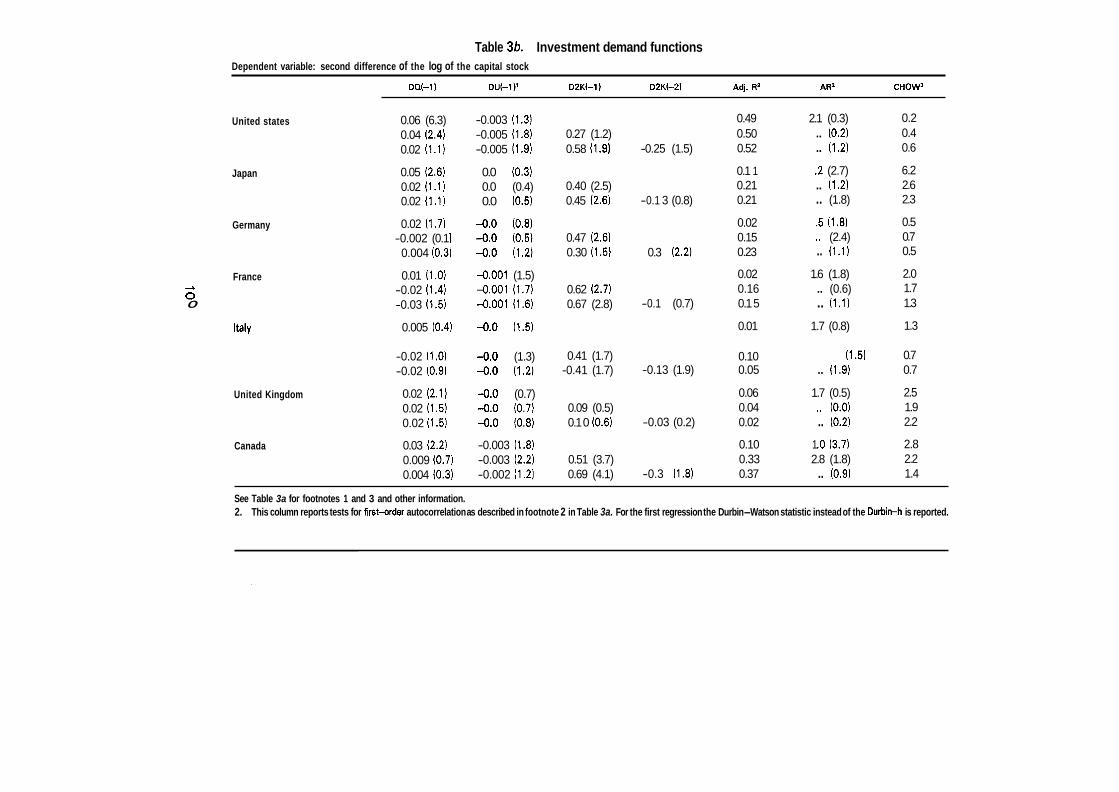
Table 3b. Investment demand functions Dependent variable: second difference of the log of the capital stock

DQ(-l) DU(-1)' D2K(-1) D2K(-2) Adj. R2 AR2 ch0w3

United states

Japan

Germany

France a 0 0

Italy

United Kingdom

Canada

0.06 (6.3) 0.04 (2.4) 0.02 (1.1)

0.05 (2.6) 0.02 (1.1) 0.02 (1.1)

0.02 (1.7) -0.002 (0.1

0.004 (0.3)

0.01 (1.0) -0.02 (1.4) -0.03 (1.5)

0.005 (0.4)

-0.02 (1 .O) -0.02 (0.9)

0.02 (2.1) 0.02 (1.5) 0.02 (1.5)

0.03 (2.2) 0.009 (0.7) 0.004 (0.3)

-0.003 (1.3) -0.005 (1.8) -0.005 (1.9)

0.0 (0.3) 0.0 (0.4) 0.0 (0.5)

-0.0 (0.8) -0.0 (0.5) -0.0 (1.2)

-0.001 (1.5) -0.001 (1.7) -0.001 (1.6)

-0.0 (1.5)

-0.0 (1.3) -0.0 (1.2)

-0.0 (0.7) -0.0 (0.7) -0.0 (0.8)

-0.003 (1.8) -0.003 (2.2) -0.002 (1.2)

0.27 (1.2) 0.58 (1 -9)

0.40 (2.5) 0.45 (2.6)

0.47 (2.6) 0.30 (1.5)

0.62 (2.7) 0.67 (2.8)

0.41 (1.7) -0.41 (1.7)

0.09 (0.5) 0.1 0 (0.6)

0.51 (3.7) 0.69 (4.1)

-0.25 (1.5)

-0.1 3 (0.8)

0.3 (2.2)

0.50 0.52

0.1 1 0.21 0.21

0.02 0.15 0.23

0.49 2.1 (0.3) .. (0.2) .. (1.2)

.2 (2.7)

.. (1.2)

.. (1.8)

.5 (1.8)

.. (2.4)

.. (1.1)

0.02 1.6 (1.8) 0.16 .. (0.6)

-0.1 (0.7) 0.1 5 .. (1.1)

0.01 1.7 (0.8)

0.10 (1.5) -0.13 (1.9) 0.05 .. (1.9)

0.06 1.7 (0.5) 0.04 .. (0.0)

-0.03 (0.2) 0.02 .. (0.2)

0.10 1 .o (3.7) 0.33 2.8 (1.8)

-0.3 (1.8) 0.37 .. (0.9)

0.2 0.4 0.6

6.2 2.6 2.3

0.5 0.7 0.5

2.0 1.7 1.3

1.3

0.7 0.7

2.5 1.9 2.2

2.8 2.2 1.4

See Table 3a for footnotes 1 and 3 and other information. 2. This column reports tests for first-order autocorrelation as described in footnote 2 in Table 3a. For the first regression the Durbin-Watson statistic instead of the Durbin-h is reported.

Tables 3a and 3b report the results using the second difference of the capital stock: they are qualitatively similar to those reported in Table 2. Taking first the results of Table 3a, output growth has a positive and significant influence on the growth rate of net investment, while the cost of capital is generally insignificant (except for the United States). However, when the contemporaneous growth rate of output is excluded from the regressions (Table 3b), adding lags of the dependent variable again tends to diminish the measured effect of the accelerator, as captured by lagged output growth. Once again, the overall specification of the equations seems to be fairly good: the R-squared is, of course, much lower than for the regressions in Table 2 (and is virtually zero for Italy and the United Kingdom), but there is little sign of autocorrelation or parameter instability.

In a sense these various regressions have much in common. They all strongly suggest that the underlying contemporaneous correlation is between output growth and investment growth (not the level of investment). The accelerator is strongly supported if contemporaneous output growth is used as a regressor, but the support is rather weaker if only lagged regressors are used, and if lags of the dependent variable are also included.

A standard interpretation of the specification used in Table 2 is that the adjustment of capital is very slow. The specification in Table 3 would naturally be interpreted as implying that the adjustment "never ends", i.e. that an increase in the level of output affects the growth rate of the capital stock permanently. It is inherently difficult to distinguish empirically between these two hypotheses because the test statistics have little power when the alternative is so close to the null. However, either interpretation would seem to spell trouble for the plausibility of the underlying investment model. It is difficult to see how the model can be reconciled with the second. As to the first, recall that adjustment lags are interpreted as being due to the costs of installing capital. How large are such costs likely to be? Put differently, how long does it take to install a piece of capital? Casual empiricism from actual investment projects suggests that installa- tion takes from much less than a year (to install machine tools, for example) to perhaps a few years (to build an entire factory). This would seem to be inconsistent with adjustment lags that are virtually indistinguishable from "forever". It could be argued that there are aggregate-supply constraints on investment expenditures - the capital-producing sector is only so large. While this is plausi- ble, it implies that the estimates reflect supply, not demand, considerations20.

C. "Non-neoclassical" explanations

In view of the disappointing performance of the simple neo-classical model, it is natural to consider other determinants of investment demand. Two candidates are profits and uncertainty.

101

1. Profits

Profits could affect investment demand through two channels. First, the neo- classical model of slow adjustment of capital implies that the existing capital stock earns quasi-rents during the transition. Indeed, these quasi-rents can be viewed as the incentive for firms to invest (if the quasi-rents are negative, they are an incentive to disinvest). In this sense, the influence of profits on investment, which in practice include both quasi-rents as well as the normal return to capital, is not inconsistent with the neo-classical model.

The second channel arises if firms face credit restrictions that drive a wedge between the cost of credit in the capital market and the shadow cost of retained earnings, or cash flow. Such restrictions can be motivated on a theoretical level by appealing to informational asymmetries between borrowers and lenders. Of course, the best way to deal with credit market failures would be to incorporate them explicitly into the firm's profit maximisation problem and attempt to estimate the resulting investment demand function directly. However, credit restrictions are commonly captured by adding cash-flow variables to the investment function, on the assumption that firms with healthy cash flows are able to finance investment internally or find it easier to borrow on capital markets.

Profit, or cash-flow, models have been found to perform no worse than, and sometimes better than, standard investment equations (e.g. Kopke, 1985; Bernanke et al., 1988, and Chamberlain and Gordon, 1989). While early cross- section studies failed to find an effect of profits on investment (Eisner, 1978), suggesting that profits had, a t best, only a short-term influence, more recent work using U.S. panel data has reversed these results (Fazzari and Athey, 1987; Fazzari et al., 1988 and Gertler and Hubbard, 1988). Finally, Devereux and Schiantarelli ( 1 989) found that new firms and firms in growing industries tended to be more liquidity constrained than others.

The business-sector profit rate2' has been rising through the 1980s and in most countries has returned roughly to levels that prevailed in the early 1970s. The unit root test reported in Annex Table A1 indicates that the profit rate is integrated of order 1. Adding cumulated profits to the cointegration tests reported above did not improve the results. Granger causality tests, using the growth of the profit rate and the three definitions of investment used above, yielded the following results: investment causes profit, but not vice versa in the United States, Japan, Germany and Canada; on the other hand, the profit rate causes investment, but not vice versa in France, Italy and the United Kingdom. On the whole, the time-series tests are not very encouraging.

This conclusion is confirmed by the regression results reported in Tables 4a and 4b, which use the same specification as the regressions reported in Table 3 - the second difference of the capital stock is the dependent variable - but adding

102

Table 4a. Investment demand functions DeDendent variable: second difference of the loo of the caDital stock

DR DR(-1)' DO D W 1 ) DU DU(-1) D2K(-1) D2K(-2) Adj. Rz AR2 CHOW3

United States 0.025 (7.1) 0.007 (3.5) .. 0.52 (5.5) 0.69 0.2 (0.1) 0.8

Japan

Germany

France

A Italy 0 0

United Kingdom

Canada

0.002 (0.5) 0.003 (0.7) 0.01 2 (2.8) 0.009 (2.0) 0.009 (2.4) 0.007 (1.8)

-0.0 (0.1) 0.001 (0.3) 0.01 3 (3.7) 0.006 (2.3) 0.005 (2.0) 0.01 (2.8)

-0.001 (0.4) -0.003 (1 .O)

0.061 (6.5) -0.0 "(0.0) 0.057 (4.9)

0.032 (1.7) 0.01 3 (3.3) 0.062 (3.0)

0.040 (4.1 ) 0.004 (1 .O) 0.032 (2.8)

0.05 (5.8) 0,003 (1.3) 0.05 (6.0)

0.060 (5.9) 0.01" (3.8) 0.073 (8.3)

0.005 (3.6) .. 0.39 (5.7) 0.85 -1.7 (-1.5) 0.02 (1.4) 0.005 (3.6) -0.001 (0.3) 0.16 (0.9) 0.09 (0.9) .. .. (-1.1)

.. -0.0 (0.2) 0.36 (2.8) 0.34 -2.3 (-1.6) -0.0 (0.1) 0.31 (2.4) 0.37 -1.2 (-0.9)

-0.02' (1.2) -0.001 (1.0) 0.004 (3.8) 0.24 (1.7) -0.15(1.2) 0.59 0.2 (0.2) .. -0.0 (0.1) .. 0.47 (3.2) 0.20 -4.1 (-2.7) .. -0.001 (1.4) 0.38 (3.0) 0.44 -0.4 (-0.4)

-0.003 (0.2) -0.001 (0.9) -0.0 (0.2) 0.29 (1.7) 0.21 (1.5) 0.42 .. (-0.1) 0.0 (0.9) 0.28 (2.0) 0.29 -0.6 (-0.4)

0.62 1.4 (1.2) .. -0.0 (0.1) .. 0.23 (2.3)

0.16 0.4 (0.0) .. -0.0 (0.2) .. 0.18 (1.2) .. -0.0 (0.9) 0.02 (0.2) 0.55 3.2 (2.9)

-0.02 (1.6) 0.0 (0.1) -0.0 (0.3) 0.39 (2.4) -0.14 (1.4) 0.64 .. (-1.5)

-0.057 (4.6) -0.0 (0.6) 0.0 (1.5) 0.37 (2.8) 0.02 (0.2) 0.71 -0.5 (-0.4)

0.007 (2.5) 0.0 (0.6) .. 0.25 (1.7) 0.13 0.6 (0.4) 0.002 (0.5) 0.029 (2.4) .. -0.0 (0.2) 0.23 (1.6) 0.22 -0.8 (-0.6) 0.003 (0.8) -0.009 (1.3) 0.026 (2.0) 0.02 (1.4) -0.0 (0.3) -0.0 '' (0.8) 0.16 (0.9) 0.02(0.1) 0.20 .. (0.7) 0.01 6 (3.8) .. -0.001 (0.9) .. 0.66 (5.4) 0.47 0.6 (0.4) 0.01 2 (2.4) 0.022 (1.7) .. -0.002 (1.2) .. 0.62 (5.1 ) 0.49 0.8 (0.6)

0.4 1.4 0.7 2.2 2.1 0.3 1.2 1 .o 1.6 2.9 2.5 0.4 6.2 1.7

1.3 1.1 0.8 2.7 2.3

0.011 (1.81 0.0 (0.11 0.021 (1.3) 0.0 (0.1) -0.002 (1.3) 0.0 (0.1) 0.70 (4.0) -0.15 (0.9) 0.45 .. (0.5) 1.2 Definition of variables: as in Table 2, except D2K denotes the second difference of the log of the capital stock and DR denotes the first difference in the log of the profit rate. The profit rate is business sector value added less the wage bill and a correction for the labour income of unincorporated businesses, all divided by the business-sector capital stock. Sample period: 19681 to 198811 (semi-annual data). All regressions have a constant term. Absolute values of t-statistics are reported in parentheses. 1. Numbers reported as 0.0 or -0.0 are less than 0.001 in absolute value. 2. This column reports two tests for first-order autocorrelation. The first figure is the Durbin-h statistic (represented by an ellipsis if imaginary, as in the third regression for the United

States). The figure in parentheses is from an alternative test involving a regression of the investment equation residuals against their own lag and all explanatory variables. The figure reported is the absolute value of the t-statistic of the coefficient of the lagged residual, which, if significant, indicates autocorrelation.

3. This column reports the F-statistics for a break in 19781. Critical values at 5 per cent are F(4.30) = 2.7; F(5.30) = 2.5; F(6.30) = 2.4.

Table 4b. Investment demand functions Dependent variable: second difference of the log of the capital stock

DW-1) DU-1) DU(-1)’ 02K(-1) D2K(-2) Adj. R2 AR2 ch0w3

United States 0.01 3 (2.3) 0.007 (1.0) 0.005 (0.7)

Japan 0.01 5 (3.2) 0.014 (3.0) 0,015 (3.1)

Germany 0.005 (1.2) 0.006 (1 -3) 0.008 (1 -9)

-. France 0.002 (0.5) 0 0.002 (0.6)

0.002 (0.5) P

Italy 0.001 (0.3) 0.004 (0.9) 0.004 (0.8)

United Kingdom 0.001 (0.4) -0.002 (0.6) -0,002 (0.6)

Canada 0.007 (1.4) 0.007 (1.2) 0.004 (0.6)

0.029 (1.3) 0.01 6 (0.7)

0.007 (0.3) 0.009 (0.4)

-0.009 (0.7) -0.006 (0.4)

-0.022 (1.2) -0.023 (1.3)

-0.027 (1.4) -0.024 (1.2)

0.021 (1.4) 0.021 (1.4)

0.001 (0.1) 0.0 (0.1)

-0.005 (1.8) -0.004 (1.4) -0.005 (1.6)

0.001 (1.1) 0.001 (1.0) 0.001 (1.1)

-0.0 (0.4) -0.0 (0.2) -0.0 (0.9)

-0.001 (1.7) -0.001 (1.5) -0,001 (1.4)

-0.0 (1.4) -0.0 (1.2) -0.0 (1.1)

-0.002 (0.4) -0.0 (0.8) -0.0 (0.9)

-0.003 (1.8) -0.003 (1.8) -0.002 (1.1)

0.49 (3.2) 0.29 (1.3) 0.56 (1.9)

0.25 (1.8) 0.23 (1.5) 0.29 (1.8)

0.41 (2.8) 0.49 (2.7) 0.27 (1.5)

0.34 (1.9) 0.53 (2.2) 0.57 (2.3)

0.19 (1.1) 0.43 (1 -8) 0.43 (1.8)

0.24 (1 -4) 0.13 (0.7) 0.1 3 (0.7)

0.48 (3.7) 0.48 (3.4) 0.65 (3.5)

-0.22 (1.3)

-0.16 (1.1)

0.37 (2.6)

-0.08 (0.5)

-0.1 2 (0.8)

-0.02 (0.1)

-0.26 (1.4)

0.49 0.50 0.51

0.37 0.35 0.36

0.17 0.16 0.27

0.1 1 0.13 0.1 1

0.03 0.05 0.04

-0.0

-0.0 0.02

0.36 0.34 0.36

.. (0.8)

.. (-0.1)

.. (-0.9)

-0.3 (0.2) -0.7 (0.2)

.. (-0.1)

-4.8 (-3.0) .. (-2.9) .. (0.1)

.. (-1.3)

.. (-1.1)

.. (-1.6)

.. (-1.4)

.. (-2.1)

.. (-2.6)

.. (0.1)

.. (0.4)

.. (0.3)

1.9 (1.4) 2.4 (1.4) .. (1.0)

0.6 0.3 0.5

0.6 1 .o 1 .o 0.4 0.4 0.3

1.6 1.5 1.2

0.5 0.6 0.6

0.9 1.6 1.7

3.0 2.3 1.7

See Table 4a for footnotes 1, 2 and 3.

the percentage change of the profit rate as an explanatory variable. This specification assumes that a higher level of the profit rate leads to more net investment (rather than to a higher desired capital stock). Table 4a reports the specification using contemporaneous regressors. While the profit variable is always significant if entered alone, it remains significant only in Japan, France and Canada if output growth is included as well - contemporaneous output growth is significant in all regressions except for Canada. Table 46 reports the specification excluding contemporaneous regressors. Lagged profits are insignificant in all countries except the United States (but only in the absence of a lagged output term) and Japan. Thus, these results provide little support for an independent role for profits in explaining investment.

2. Uncertainty

Risk-averse firms will reduce the value they place on returns to investment as uncertainty increases and firms will tend to delay investment decisions in order to accumulate more information, even if they are risk-neutral. There is little empirical work measuring the quantitative importance of uncertainty on investment demand, although Artus (19841, Poret (1986) and Lomax (1990) found some evidence that it reduced investment.

Several proxies suggest that the climate for investment decision-making was, if anything, somewhat less uncertain in the second half of the 1980s than in the 1970-83 period. An ex post measure of uncertainty is the variability of key macroeconomic variables, on the presumption that higher volatility implies larger forecast errors. Table 5 presents standard deviations of the rates of change of industrial production, producer prices, the real long-term interest rate and the nominal effective exchange rate for most OECD countries and for 1960-82 and 1983-89. For most countries the volatility of the first three variables was lower in the 1983-89 period. In contrast, nominal exchange rates tended to be more volatile recently22.

Direct evidence on the possible effects of uncertainty can be obtained by comparing actual investment expenditures with investment intentions, as measured by surveys. It is assumed that firms' reported intentions are based on predictions of the factors relevant to the investment decision. As these factors become more predictable, the actual outcome should be closer to the intentions. As is shown in Table 6, the revisions tended to be slightly smaller in the period 1983-88 than in other sub-periods. Among the larger countries, exceptions are France, where they were about the same as in the 1979-82 period, and Canada, where they were smallest in the 1974-78 period. Among the smaller countries, data from the 1970s was available only for Belgium and Luxembourg: the size of the revisions fell in Belgium, and revisions were very volatile in Luxembourg.

105

Table 5. Volatility indicators’

Real long-term Nominal effective Producer prices exchange rate interest rate2 Industrial production

United States 1960s-82 1983-89

Japan 1960s-82 1983-89

Germany 1960s-82 1983-89

France 1960s-82 1983-89

Italy 1960s-82 1983-89 ,

United Kingdom 1960s-82 1983-89

Canada 1960s-82 1983-89

Australia 1960s-82 1983-89

Austria 1960s-82 1983-89

Belgium 1960s-82 1983-89

Denmark 1960s-82 1983-89

2.31 1.24

3.53 2.41

1.86 1.72

2.94 0.95

3.16 1.66

2.1 1 1.38

1.93 1.51

1.97 2.07

1.89 1.24

2.31 1.57

- -

0.93 0.44

1.62 0.67

0.72 0.46

1.22 0.65

1.84 0.75

1.70 0.97

0.98 0.27

1.28 0.67

1.06 0.77

0.91 0.61

1.35 0.69

2.20 1.54

4.43 0.90

0.93 0.81

1.93 0.82

4.06 1 .oo

3.94 1.51

I .87 1.30

3.42 2.16

1.64 1.11

2.79 0.92

3.20 0.93

1.87 3.35

3.20 4.72

1.98 1.43

2.13 1.54

2.23 1.49

2.71 3.93

1.49 1.66

3.24 5.72

1.04 0.71

1.41 1.04

1.41 1.27

1. Standard deviation of quarterly rates of change over each sub-period. 2. Nominal rate less year-on-year rates of change in consumer prices.

106

Table 5 (continued)

Real long-term Nominal effective interest rate2 exchange rate Industrial production Producer prices

Finland 1960s-82 1983-89

Greece 1960s-82 1983-89

Ireland 1960s-82 1983-89

Netherlands 1960s-82 1983-89

New Zealand 1960s-82 1983-89

Norway 1960s-82 1983-89

Portugal 1960s-82 1983-89

Spain 1960s-82 1983-89

Sweden 1960s-82 1983-89

Switzerland 1960s-82 1983-89

2.88 1.34

2.54 2.61

2.54 2.95

1.81 2.66

- -

2.37 4.75

3.33 1.95

9.56 11.26

2.33 2.04

2.55 2.30

1.33 0.68

2.62 2.05

1.92 0.78

1.12 0.57

1.46 1.67

1.21 0.62

2.80 2.1 8

1.73 0.95

1.12 0.83

0.79 0.58

3.92 2.44

6.61 3.86

3.28 2.00

2.03 0.86

3.67 3.62

2.23 1.18

6.91 4.55

5.04 2.10

2.13 1.36

1.83 0.94

2.59 0.97

2.32 4.17

1.39 2.12

1.25 1.37

2.33 5.28

1.21 1.74

2.73 2.61

2.78 2.69

2.29 0.97

2.69 2.1 7

1. Standard deviation of quarterly rates of change over each sub-period. 2. Nominal rate less year-on-year rates of change in consumer prices.

107

Table 6. Revisions in investment intentions'

Average over the 983-1 988 entire sample period 1960s-1973 1974-1 978 1979-1 982

United States 3.3 2.5 3.7 1.7 2.9 Japan 2.6 4.9 3.5 3.5 3.6 Germ any 2.5 3.1 2.3 2.2 2.5 France 3.8 2.3 1.9 2.0 2.6 Italy 6.4 4.9 8.7 5.1 6.1 United Kingdom 4.B2 4.1 2.9 3.8 Canada 3.2 8.3 4.6 4.8

Belgium 3.8 7.8 5.5 5.7 Luxembourg 10.5 24.1 6.5 24.5 17.1 Netherlands 3.0 4.0 3.4 Ireland 10.3 23.7 16.9

1. Average absolute value of revisions in investment intentions (normalised by subtracting the average errors over the entire sample period). Revisions are the difference between the realised rate of increase in nominal fixed investment, as declared by firms at the beginning of the following year, and the rate which was expected at the beginning of the current year.

2. 1975-78. Sources: United States: US. Department of Commerce, Bureau of the Census.

Japan: Bank of Japan, Short-Term Economic Survey of Enterprises in Japan. France: INSEE, Enqugte sur I'investissement dans I'industrie. Canada: Statistics Canada: Public and Private lnvestment. Other countries: European Community lnvestment Surveys.

D. Conclusions on investment demand

This section has examined variables identified by standard investment theories as being key factors in investment demand - output (or expected demand), the cost of capital, profits and uncertainty - paying particular attention to the first two. Although estimating investment demand functions has always been a challenge, many investigators have succeeded in finding some empirical support for both variables, especially output. Empirical support has also been found in the literature for the role of profit, or cash-flow, variables.

However, the statistical analysis presented in this section suggests that the neo-classical model, even when augmented with profit and uncertainty variables, is probably not consistent with the data. The regression analysis provides support for the accelerator, but mainly when the current growth rate of output is used as a regressor. The profit rate receives only limited support - its current growth rate must be used as a regressor and the current growth rate of output must be excluded. There is little support for any role for the cost of capital. Attempts to

108

add measures of output, price, interest-rate and exchange-rate volatility (as proxies for uncertainty) to the neo-classical investment model proved unsuccess- ful. Taken together, these results suggest that it would be unwise to draw strong inferences on the basis of the estimated coefficients of investment demand models.

111. PUBLIC POLICY AND INVESTMENT

This section discusses the role of government policies towards investment in the 198Os, particularly in the United States, where there is a large literature on the role of investment incentives. There was a general movement in the OECD countries during these years towards broader bases and lower rates in both household and corporate taxation23. As a result, direct incentives to investment were reduced while statutory corporate tax rates fell.

A. Econometric studies

Bosworth (1 9841, in a survey of the literature, concluded that taxes probably have a significant, but small, effect on investment, but that the evidence for this proposition was weak. Investigators in other countries have also concluded that tax policy has a small effect on investment demand: see Muet and Avouyi-Dovi (19871, who studied the French tax reforms of 1982, and Sumner (1986) and Devereux (1 989) who analysed the U.K. reforms in 1984 which reduced the top corporate tax rate from 52 to 35 per cent and eliminated accelerated depreciation. Feldstein has been perhaps the strongest proponent of the importance of taxation - see Feldstein (1 9821, Feldstein and Jun (1 9871, and Sumner (1 9881, who refined Feldstein's earlier estimates.

The most far-reaching tax reforms in the 1980s were undertaken in the United States; these have also been by far the most intensively studied. In 198 1, the Economic Recovery Tax Act (ERTA) introduced accelerated depreciation and extended investment tax credits with the explicit purpose of stimulating investment and capital formation. A year later, some of this support for investment was withdrawn in the Tax Equity and Fiscal Responsibility Act (TEFRA), which eliminated the accelerated depreciation introduced under ERTA and reduced the gener- osity of the investment tax credit. TEFRA also substantially reduced the disparity in effective tax rates by asset type (Boskin, 1988, Table 31, with the objective of improving resource allocation. Investment incentives were further cut back by the Tax Reform Act (TRA) of 1986. The accelerated depreciation and the 10 per cent investment tax credit were eliminated, and depreciation schedules were made less

109

generous by lengthening tax lives. On the other hand, the corporate tax rate was reduced. Nevertheless, the overall effect was probably an increase in the effective tax rate.

The U.S. tax reforms had large effects on the cost of capital and therefore provide a "laboratory experiment" of the effect of taxation policy on investment demand. Unfortunately, there were large movements in output growth at the same time and, generally, in the same direction (in terms of the theorised effect on investment). Much econometric work in this area has therefore been devoted to disentangling the effects of output and the cost of capital on investment.

In general, the conclusions are similar to those reached in the literature on the broader issue of the determinants of investment demand: output was more important than the tax reforms. Bosworth (1985) assessed the 1981 and 1982 reforms and found that they did not have much influence on the pick-up of investment demand in the 198 1-84 period. In fact, he found that the investment recovery was the strongest in sectors where the tax changes were relatively minor. Corker et a/. (1988) attributed only a "distinctly subsidiary" role to the three reforms, arguing that output was the dominant factor. Boskin (19881, in contrast, concluded that tax policy "is an important (but hardly exclusive) deter- minant of investment", and that the 1981 and 1982 U.S. tax reforms had a substantial influence in stimulating investment.

B. Applied general equilibrium (AGE) models

The AGE methodology often does not provide direct empirical evidence of the effects of taxes on investment decisions. Rather, functional forms and param- eters drawn from theoretical or econometric work are imposed, and the simulation results are conditional on them. In particular, AGE models are "calibrated", often to one year's data, on the assumption that the economy being modelled was in equilibrium in that year. This is quite different from standard practice in econometric model building, where the model is expected to explain, or "track", actual data over a substantial sample (and sometimes even beyond the sample).

Another limitation of many AGE models is an inadequate treatment of intergenerational considerations. This is important because most policy experi- ments imply significant redistributions of resources across different generations. Static models cannot, of course, deal with this issue at all, and multi-sectoral dynamic models typically treat the household sector as an infinitely-lived represen- tative consumer. More aggregated dynamic models can address intergenerational issues directly by using the overlapping-generations structure, but have a corre- spondingly more limited ability to deal with such policy issues as the intersectoral distribution of capital.

110

Pereira and Shoven ( 1988) and Henderson ( 1989) provide good summaries of several major AGE studies of the 1986 Tax Reform Act (TRA) and of their underlying assumptions. Differences in model specification and in the provisions of the TRA which were incorporated in the models give rise to a wide range of conclusions about the effects of the tax reform. For example, many studies include features of the TRA that have no direct bearing on capital taxation (e.g. the reduction and simplification of personal income tax rates). It is therefore difficult to isolate the effects of the changes to the corporate tax system from those of other changes.

AGE models can be divided into two classes: static and dynamic. The former do not model the adjustment costs involved in moving from the old to the new equilibrium and necessarily have a very simplified treatment of households' intertemporal choices. They have therefore been used primarily to assess the long- term trade-off between: i) the reduction in overall investment incentives, which lowers the capital stock, output and, given the definitions used in these models, economic welfare; and ii) the improvement in the allocation of capital across sectors, which raises economic welfare.

In general, simulation studies using static models conclude that the TRA increased welfare, as the allocative effects dominated (see Fullerton, Henderson and Mackie, 1987 and Gravelle, 1989). However, Grubert and Mutti (1987) and Galper et a/. ( 1 988) came to the opposite concl~sion~~. At the same time, the estimated static gains from eliminating tax distortions due to differential treatment of various asset classes are quite small as a fraction of GDP, a result which is typical of static AGE models.

Dynamic models have several advantages over static ones for assessing the effects of tax reforms, since capital accumulation is by nature a dynamic process. They can focus on the role of adjustment costs which, as was mentioned above, play a key role in the theory of investment demand. In general, adjustment costs slow the response of investment to changes in the cost of capital and thereby reduce the present value of the gains from higher investment incentives. Adjust- ment costs can also limit the mobility of capital across sectors, thereby reducing the gains from the elimination of intersectoral tax wedges. Dynamic models can also capture the difference between capital that is already installed and new, or marginal, capital. This distinction is important in the analysis of policies, such as the investment tax credit, that apply only to new capital. Finally, work with aggregate dynamic AGE models suggests that a large part, but not all, of the steady-state increase in the capital stock amounts to a transfer of resources between generations, rather than a gain in aggregate economic efficiency. Dynamic models suggest that the combination of lower corporate income taxes and elimination of investment tax credit depresses long-run capital intensities and welfare, but a t the same time they generate intersectoral efficiency gains (Bovenberg and Goulder, 1989; Bovenberg, 1988; Goulder and Summers, 1988;

111

and Jorgenson and Yun, 1989). with the net effect tending to be an increase in welfare (Bovenberg and Goulder, 1989; and Jorgenson and Yun, 1989).

Given that the elimination of the investment tax credit has generally been found to imply substantial reductions in investment and long-run capital intensities, with relatively smaller effects on intersectoral efficiency, some authors have argued in favour of re-introducing it (Bovenberg and Goulder, 1989; Goulder and Summers, 1988). However, Pereira ( 1989) shows that the effects of introducing an investment tax credit depend on how it is financed. With deficit financing, the boost in investment can be more than offset by the combination of financial crowding-out and intersectoral efficiency losses. Jorgenson and Yun ( 1989) argue that major benefits could be achieved by indexing the capital tax base and by shifting the tax burden from corporate capital to household capital, by, for example, eliminating the mortgage interest deduction.

IV. THE BENEFITS OF INVESTMENT

This section briefly considers the channels through which greater investment

i) More investment means a larger capital stock and therefore increased productive capacity. Some recent developments in growth theory suggest that the return to extra investment in terms of both expanded productive potential may be far greater than standard models predict. A higher rate of gross investment could allow the more rapid adoption and diffusion of new production methods and techniques, thereby raising productivity.

An important qualification to all arguments for more investment is that it implies less current consumption, given current production possibilities. Thus, while more investment now might add to the welfare of future generations, it is at the expense of the current generation, which must save to finance it. Such a trade-off cannot be evaluated on purely economic grounds because there is no generally accepted way to make interpersonal or intergenerational welfare comparisons.

could increase aggregate output in the longer run:

ii)

A. Capital formation

Investment raises the productive capacity of an economy by increasing the stock of capital. Standard growth models have two key implications for the importance of capital formation on potential output. First, the elasticity of output

112

with respect to capital is only about one-third for the typical OECD country. Thus, most economic growth must be attributed to increases in employment and to technical change. In the absence of a convincing explanation of its movements, the latter is typically assumed to be exogenous. Second, an increase in the level of the investment-output ratio will ultimately increase the level, not the growth rate, of the capital-output ratio. The reason is twofold: first, depreciation eats up more and more of the extra investment as the stock of capital increases; and second, the output from successive units of capital (i.e. the marginal product of capital) falls25.

However, it has been argued recently that this view of the growth process is incorrect and that an increase in the level of investment or the saving rate (or the efficiency of the use of factor inputs) can increase the growth rate, not just the level, of output permanently. This "new" theory of economic growth emphasises the role of investment in both physical and human capital (see, for example, Lucas, 1988; Scott, 1989 and Romer, 1989b). For example, R&D produces knowledge that can be used simultaneously by more than one firm (it is said to be non-rivalrous). Thus, an increase in the level of R&D would lead to a rise in the flow of knowledge and the rate of growth of technical change. Moreover, to the extent that new production possibilities are embodied in new capital, investment makes further R&D possible. If these effects are large enough, an increase in net investment could be sustained indefinitely because the marginal product of capital would not diminish with capital deepening.

If the new growth theories are correct, the effects of many public policies would be much larger than those calculated using the standard economic frame- work26. In particular investment incentives could have large pay-offs in terms of increased economic growth. Alternatively, distortionary policies might have much larger effects on the economy than previously thought, since their efficiency losses would be compounded over time through permanent effects on the growth rate2'. For instance, removal of trade barriers can boost profits from innovating by increasing the size of the market over which R&D costs can be spread. The link between openness to trade and long-run growth has been analysed by Grossman and Helpman (19891, Krugman (1988) and Romer (1990). Baldwin (1989) argued that the positive welfare effects of the EC single market of 1992 may have been greatly underestimated by the Cecchini Report ( 1988) which, focusing only on the static gains, concluded that the level of EC income could rise by 2.5 to 6.5 per cent in the long run. In contrast, using a very simple computable "new" growth model with a constant aggregate saving rate, Baldwin concluded that the impact of 1992 could be to increase the EC growth rate by 0.3 to 0.9 per cent per annum. This implies that the level of EC income would be 3 to 9.4 per cent higher after ten years, 6 to 19.6 per cent higher after twenty years, and so forth.

In view of the importance of their implications, it is essential to examine critically the evidence in support of the new growth models. Unfortunately,

113

empirical investigations are still at a primitive stage. There is as yet little direct evidence about either the assumptions on which the models are based - increasing returns to scale, technological externalities, human capital spillovers, and so forth - or the implications of the models. This is due in part to the novelty of this line of research and also to the fact that many of the variables on which the new growth theories hinge are either unobservable or poorly measured - human capital, technological innovations and productive public investment being obvious examples.

The available evidence is of two sorts. The first examines the question of aggregate returns to scale directly, and the second, which is more common, tests the /theories indirectly by examining cross-country correlations. In all OECD countries, the labour-output ratio (the inverse of labour productivity) falls markedly over time. In contrast, the capital-output ratio is relatively stable. Standard growth models appeal to technical change, which is usually assumed to augment labour only, to explain these stylised facts. By contrast, the "new" growth theorists explain this by imposing an output elasticity of capital in the aggregate production function which is approximately unity. Since labour's coefficient is positive, this implies aggregate increasing returns to scale. Romer ( 1987) and Baldwin (1989) argue that the "new" theory is a t least as consistent with the long run data as the standard theory.

The second sort of evidence, from cross-country regressions, attempts to show that countries with faster output growth have also had higher levels of variables that are hypothesised to affect growth (private or public investment, for example, or education) (see Romer, 1989a; Easterly and Wetzel, 1989; and Barro, 19896, 1990). Although the evidence is suggestive, it is far from decisive. In particular, given the poor state of knowledge about the determinants of growth, it is difficult to control for "all other factors" in such regressions.

B. Embodiment effects

An important theme of the "new" growth theory is the importance of spillovers from investment. This notion is reminiscent of the much older hypothesis that new inventions and techniques are embodied in new machinery. Although the embodiment hypothesis does not necessarily imply the existence of spillovers, the existence of either effect implies that rapid rates of gross investment ought to be associated with higher productivity growth.

Perhaps the most dramatic example of the embodiment of new technology is the rapidly increasing importance of computer and related investment. In this case, simple observation provides evidence that new technology is embodied in new types of capital - computers embody the technology of fast electronic computing, just as adding machines embodied the older technology of mechanical

114

computing. A "puzzle" has arisen, however, in that there appears to be no strong productivity pick-up associated with all this investment. Although as yet the puzzle has not been satisfactorily resolved, several possible solutions have been suggested:

i)

ii)

iii)

There is no puzzle, since the accumulated investment in computers has not yet raised the capital stock sufficiently to have had much effect in the aggregate. Romer ( 19881, on the basis of a back-of-the-envelope calcu- lation, suggested that computer investment may have raised output growth by only about one-twentieth of 1 per cent per annurn, which is far too small to be detected. Moreover, in those countries using the BEA- type quality correction (i.e. the United States, Canada and Australia), computers are, by definition, no more productive than any other piece of capital. Productivity has risen, but the major impact of computers has been in sectors - primarily service sectors and the government sector - where output is notoriously difficult to measure. However, there is little evidence that output measurement errors in the service sectors have increased over time. Productivity has not risen because of inadequacies in training, application software or organisational restructuring. However, this hypothesis comes very close to arguing that technical change is, at least in part, disembodied.

Despite the common-sense appeal of embodiment, supporting evidence has often been difficult to find in aggregate economic data. There is, however, indirect evidence consistent with embodiment. For example, Englander and Mittelstadt (1 988) found that capital growth tends to contribute more to output growth than its share in income would suggest. Also, many "vintage" models -which assume embodied technical change - have been successfully estimated, thus providing further indirect support. Finally, there is a substantial literature establishing a relationship between R&D and productivity, although this work has not estab- lished that the fruits of R&D are embodied in capital28.

A simple and direct test is to relate a productivity measure to a proxy for the amount of embodiment. If time series of total factor productivity growth and the "capital replacement rate", which is the ratio of gross investment to the capital stock are compared, there is a very strong cyclical correlation but, for most countries, no obvious lead-lag relationship that would be expected if embodiment effects were an important explanation of trend changes in productivity growth (see Ford and Poret, 1990, for more details). One way of eliminating cyclical effects is to examine cross-section data, averaged over a sufficiently long period of time. Wolff ( 1987) does this, and concludes that there is evidence in favour of embodiment.

115

V. CONCLUSIONS

The pattern of investment in most OECD countries in the 1980s was characterised by relatively weak levels of business net investment as a fraction of output. These developments were reflected in flagging capital-output ratios. At the same time, it would appear that more investment would be beneficial for a number of reasons - output and consumption possibilities would rise, and greater public and private investment could promote more rapid economic growth via embodiment or spillover effects. Taken at face value, these conclusions imply that government intervention that spurred higher investment could raise overall welfare.

This paper has examined the extent to which the fundamental time-series properties of investment, output and the cost of capital are consistent with the underlying theory. The conclusions are largely negative. There seems to be no trend, or cointegrating, relationship among these variables. Even cyclical relationships may not be robust, as revealed by regression analysis and "causality" tests: for most of the OECD economies examined, the best explanation of current investment growth may be its own past.

Three factors suggest that incentives to invest may not increase overall welfare as much as has on occasion been claimed. First, investment can rise only if saving rises. If it does not, government action to raise the demand for investment goods - for example, by introducing investment tax reliefs - will tend to: i) raise real interest rates or the price of investment goods, thereby offsetting the effect of the tax changes on the cost of capital; or ii) generate a deterioration in the current account if the higher investment is financed by savings from abroad.

Second, there is considerable doubt that such incentives do, in fact, raise investment demand. The standard theory of investment demand implies that investment incentives will cause firms to substitute towards capital-intensive production techniques, at least as long as the production function exhibits a non- zero elasticity of substitution. However, as discussed in detail in Section II, this theory rests on shaky empirical foundations. Much of the literature on investment demand has emphasised the difficulty in estimating robust cost-of-capital effects. The intensive examination of the U.S. experience with the introduction and with- drawal of tax incentives in the 1980s has generated a wide range of opinion on their effectiveness.

Third, even if government incentives raise investment and the capital stock, they may actually reduce potential output and welfare by causing capital to be misallocated. There is evidence that investment incentives in the U.S. had allocative costs and the literature on capital subsidisation suggests the problem is widespread (see Ford and Suyker, 1990).

116

An important implication of the inability to convincingly and robustly model business sector investment behaviour is that concrete policy advice regarding the effects of investment incentives must be viewed with caution. Tax breaks, such as accelerated depreciation and investment tax credit, reduce the cost of capital, which may increase investment and the capital stock. Alternatively, they may do no more than erode the corporate tax base, leaving the capital stock unchanged in the end.

117

NOTES

1.

2.

3.

4.

5.

6.

7.

Although this paper focuses on investment demand, actual investment depends, in part, on supply (i.e. on savings). Dean et a/. (1 990) review the recent trends in savings in the OECD countries.

In this paper, net investment is defined as gross investment less scrapped capital. Cumulating net investment yields the gross capital stock, the concept used throughout this paper. This definition of net investment is different from the standard definition, which is gross investment less depreciated capital.

There is also the "accounting effect" attributable to the increase in the capital-output ratios in most OECD countries over the past two or three decades. A higher capital-output ratio, all else equal, implies that a larger fraction of gross investment must be devoted to replacing scrapped capital.

One reservation with using national accounts data to make cross-country comparisons is that they reflect differences in both quantities and relative prices. The latter can be eliminated by using international purchasing power parities. These are described in Hill (1 986). The OECD has calculated PPPs at a high level of disaggregation for 1985. Using these instead of exchange rates to make international comparisons does not significantly affect the overall ordering of high and low investment countries, although the rankings of some countries are changed. See Ford and Poret (1990) for more details.

The hedonic methodology involves measuring selected characteristics of computers (processor speed, memory and so forth) and, on the basis of regressions which link the prices of machines to these characteristics, assigning monetary values ("shadow prices") to each characteristic. A computer is treated as a bundle of these characteristics and its quality is adjusted accordingly. By contrast, the matched-model procedure captures quality changes by following the evolution of the prices of similar models over time. When new models are introduced, their price relative to existing older models is assumed to reflect quality differences, and is used to extend the quality-adjusted price index. However, accounting for quality change has given rise to another measurement problem. The combination of a falling price and a rising share of computer investment implies that measured real investment growth is sensitive to the national accounts base year. This complicates the analysis of both investment patterns and the evolution of productivity over the past two decades. For example, in the case of the United States, if a chain- weighted (Tornqvist) index were used instead of the 1982 base year, measured real investment growth ("producers' durable equipment") would have been almost 0.5 per cent per year lower between 1979 and 1988 than was recorded in the national accounts (Baily and Gordon, 1988, Table 1 1). See Ford and Poret (1990) for details. Given the availability of data, adjustment can be made for only a few countries. Moreover, the adjustment is somewhat crude. No account

118

8.

9.

10.

11 .

12.

13.

14.

15.

16.

is taken of differences in the definition and mix of computer equipment from country to country, nor is a distinction made between imported computers and those produced domestically. However, the effects of such refinements are likely to be quite small relative to those of the sharp decline in the quality-adjusted price of computers.

In Keynesian models, output is generally interpreted as "demand". However, as the accelerator is based on a technical relatibnship (i.e. the production function), it could also work through the supply side. Real business cycle models typically assume investment and output are supply driven. For a recent debate on real business cycles, see Mankiw (1 989) and Plosser (1 989).

Algebraically, c = p*(r + d)*(l - k - t*z)/( l - t), where the real cost of capital in terms of output (c) depends on the real purchase price (p), the cost of funds (r), the depreciation rate (d), the investment tax credit rate (k), the discounted present value of depreciation allowances (z) and the corporate income tax rate (t). If the firm were constrained in capital markets, its cost of capital would also depend on the method of financing - an issue discussed below. It may be thought that the observed correlation is built into the data, since one of the "components" of output is investment itself. However, subtracting investment from output has little effect. Chart 2 actually shows the second difference of the log of the capital stock, which is the dependent variable in many of the regressions presented below. However, to avoid clumsiness, when speaking of data the first difference of the log of the capital stock will be referred to as "investment" and the second difference as the "growth in investment", unless it might be ambiguous to do so.

Chevallier er a/. (1 989), using panel data, assumed that the expected inflation rate was the same for all firms and therefore did not have to be measured. They found strong effects of firm-specific interest rates on investment. Auerbach and Hines (1987) illustrated this point in the context of a simulation model of investment demand. A comprehensive discussion of Tobin's Q and estimates of it for nine OECD countries, are presented in Chan-Lee (1 986). Unfortunately, his data end in the early 1980s, and so shed no light on the later investment recovery.

Data for the cost of capital were constructed as follows. The cost of funds was proxied by an average of debt and equity costs, weighted by their shares in total liabilities. Debt cost was defined to be an average of short and long-term debt, weighted by their shares in total debt, less the smoothed inflation rate, as measured by the GDP deflator. Equity cost was proxied by the ratio of dividend pay-outs to stock prices. The real price of capital is the ratio of the non-residential fixed investment deflator to the GDP deflator. Due to lack of data, taxes were proxied by the effective corporate tax rate - corporate tax revenues divided by corporate profits. This measure is not the relevant statutory marginal rate. Moreover, accelerated depreciation and investment tax credits were ignored.

A series x is said to be integrated of order d (written I(d)) if the dth difference of x is a stationary series. For example, a random walk, given by x(t) = x(t-I ) + eh), where eh) is stationary, is l(1). A stationary (i.e. I(0)) series: i) has finite variance which does not depend on time; ii) is only temporarily affected by random innovations; and iii) tends to fluctuate around the mean (which may include a deterministic trend).

Two series, x and y (which must have the same order of inwration, d) are said to be cointegrated of order d-n if a linear combination of them is integrated of order n (which must be less than d). For example, two l(1) series related as y = a + b*x + e, where e is

1

119

17.

18.

19.

20.

21.

22.

23.

24.

25.

26.

I(O), are said to be cointegrated of order 1, with the cointegrating vector (a, b). The concept can be extended to more than two variables. Intuitively, if two variables are cointegrated, they have a stable long-run, or low frequency, relationship in a statistical sense. A variable, x, is said to "cause" y if knowing x helps to reduce the prediction variance of y. In practice, the test is a regression of y against its own lags and against lags of x. If the latter are collectively statistically significant, one concludes that x causes y.

Similar statistical results, apart from the causality tests (which were not done) have been obtained for France and the United Kingdom by, respectively, Glachant and Nivet (1 989) and Lomax (1 990). Instrumental variable regressions, using lags of (the log of) output and the cost of capital (and, alternatively, lags of their growth rates) as instruments, were also tried. In general, neither output nor the cost of capital had much explanatory power. However, the instruments may have been poor. Output, in particular, has frequently been characterised as a random walk, implying that its first difference is not correlated with its lagged level. An open economy need face no such supply constraints. Nevertheless, domestic residents can increase investment and maintain consumption only by borrowing from foreigners. On the one hand, capital markets may be imperfect, in which case this is reflected in the regression coefficients. On the other hand, residents may choose not to incur such debt, in which case the coefficients reflect this portfolio behaviour. This is defined as business GDP less wages, imputed proprietors' wage income and corporate taxes, divided by the business sector capital stock. Of course, it need not be the case that decreased ex post volatility in the latter half of the 1980s meant decreased ex ante prediction errors. To explore this possibility, simple ARlMA time-series models were estimated for each of the four series in the seven largest OECD countries. The standard deviations of the one-step-ahead forecasts (the data are quarterly) were used as a proxy for ex-ante unpredictability. On the whole, the evidence from, the forecast errors is consistent with that from the ex post variances. See Ford and Poret (1990, Table 12) for a summary of the changes that affected the corporate sector. Hamilton et a/. (1 989) used a static AGE model to analyse several tax options for Canada, including the 1986 "Budget Paper" proposal which comprised a reduction of the federal corporate tax rate from 36 to 29 per cent, a 25 per cent reduction in the depreciation allowance rate, the abolition of the investment tax credit and the elimination of the inventory allowance. They concluded that the impact on investment would be minor. A third implication, closely related to the first two, is that raising the capital stock per head need not increase steady-state per capita consumption. A higher capital stock requires more resources to be devoted to capital replacement and, if there is population growth, simply to maintaining the capital-population ratio. At some point, these "over- heads" exceed the extra output generated by the new capital and the output remaining for consumption falls. An empirical assessment of whether more capital would increase per capita consumption levels is extremely difficult. Abel et al. (1 989) concluded that it would for a large sample of OECD countries. These theories also imply that differences in rates of growth across countries can be explained by differences in historical policy developments. For example, King and Robson (1989) show how, in theory at least, past fiscal shocks could affect the trend rate of growth of an economy.

120

27.

28.

Another implication is that certain components of government spending, such as investment in infrastructure, may boost economic growth by enhancing the efficiency of resources, due to economy-wide increasing returns, yielding a non-linear relationship between growth and government size (Easterly, 1989). See, for example, Mansfield et a/. (1 977); Mansfield (1 980); Griliches (1 986); Bernstein (1 988); Bernstein and Nadiri (1 988, 1 989); and Lichtenberg and Siege1 (1 989).

121

Annex

STATISTICAL TESTS ON OUTPUT, CAPITAL, THE COST OF CAPITAL AND PROFITS

The unit root tests reported in Table A I are augmented Dickey-Fuller tests with second-order correction. The testing strategy, following Perron (1988), involves a sequence of tests that run from general to restricted alternative hypotheses. We begin with the alternative hypothesis of a stationary series with a time trend:

2

i=l Axt = p + P(t-T/2) + aXt-l + 2 yi AXt-i + ut Ial I

If p equals 0, there is no time trend; if a equals 0 the series has a unit root. If the series has a unit root, p is interpreted as its drift. The y-coefficients are the second-order correction terms.

The test statistic @3 jointly tests the two zero restrictions (a = p = 0) for the null of a unit root, no time trend and a drift. If it exceeds its critical value, the null is rejected, i.e. the series is deemed to be stationary, and the process stops. If not, the null respecified to have no drift and no time trend. The test statistic 4, therefore jointly tests three zero restrictions (p = a = p = 0). If it exceeds its critical value, the additional constraint of zero drift is rejected, the series is deemed to be non-stationary on the strength of @3, and the process ends. If not, further tests are carried out with more restricted alternatives. The first restriction yields an alternative of a stationary series with no time trend; i.e. the same as [a l l but without the second term. The relevant null is a series with a unit root and no drift. Therefore, the statistic @1 jointly tests two zero restrictions (p = a = 0). If it exceeds its critical value, the series is deemed to be stationary. If not, a final restricted alternative - a non-stationary series with a zero mean and no time trend - is considered, i.e. the same as [a l l but without the first two terms. The statistic t tests one zero restriction (a = 0), for the null of a unit-root. If it exceeds its critical value, the series is deemed to be stationary. Thus, only if all four test statistics lie within their critical values, or if G3 is below, and@, is above, its critical value, is the series deemed to have a unit root.

In Table AI, any test sequence that concludes that the series is stationary is marked with an asterisk. The first four columns show the results of the tests on the growth rate of the capital stock. All four test statistics lie within their critical values for all countries, implying that the first difference of the log of the capital stock has a unit root (and, therefore, that the log of the capital stock has two unit roots). The next two columns show the results for the change in the first difference of the log of the capital stock. Since this series is unlikely to have either a drift or a time trend, only $1 and, perhaps, t are relevant. In fact, for all countries, @1 exceeds its critical value and there is therefore no need to calculate t. The next four columns show the test for the log of gross investment. Only in Germany does Q3 exceed its critical value, indicating stationarity (using fourth-order correction suggests non-stationarity, however). In four other countries, @, exceeds

\

122

Table A l . Unit root tests for the seven major OECD countries

Aln KBV M l n KBV In IBV Aln IBV Aln GDPBV Aln UCC Aln R Variable:

0 3 0 2 0 1 t 0 1 t 0 3 0 2 01 t 0 1 t 0 1 t 0 1 t 0 1 t

United States (59) Japan (49) Germany (55) France (53) Italy (59) United Kingdom (57) Canada (47)

5.01 3.36 4.68 -0.19 11.36* - 4.54 5.37 - - 14.61* - 9.07' - 11.14' - 8.89' - 1.40 1.60 2.49 -1.89 5.38* - 3.88 5.41 - - 7.95* - 3.72 -1.38 10.62* - 7.94* -

- - 6.87* - 7.63* - 20.58* - 8.70* - 5.62 4.05 2.27 -1.45 6.09* - 7.09* -

1.76 1.29 0.52 -0.80 6.06' - 1.98 2.98 4.47 2.21 5.89* - 4.00 -1.45 9.78* - 4.22 -2.79* 5.57 4.20 3.51 -1.77 7.85* - 3.69 3.24 1.80 1.47 8.26* - 10.26* - 6.28* - 12.41* - 1.34 0.93 1.20 -0.72 5.28* - 2.04 4.20 4.53 2.91 11.17* - 5.62* - 12.93* - 9.65* - 3.77 2.69 3.00 0.36 7.85, - 4.81 6.41 - - 6.23* - 8.05' - 10.70* - 9.65* -

In brackets: number of observations (semi-annual data). An asterisk denotes that the non-stationarity hypothesis is rejected; that is, the series are stationary.

Definition of the variables

KBV: real capital stock; IBV: real gross fixed investment; GDPBV real value-added: UCC: real user cost of capital; R: rate of profit: In denotes the logarithm, A is the first difference operator and M is the second-difference operator. All variables are for the business sector.

Critical values of the @ and t statistics do not follow the usual t- and F-distributions. For 50 observations, the critical value for the t-statistics at the 5 per cent level is -1.95 (Fuller (1976), Introduction to Statistical Time Series, p. 373). The critical values for 0 3, @ 2 and @ 1 are 6.73, 5.13, 4.86 (Dickey and Fuller, 1981, Econometrica 4, p. 1063).

A

N G)

its critical value, implying that the log of gross investment is non-stationary. For France, Italy and the United Kingdom all four statistics lie below critical values, implying non-stationarity as well. All other variables tested proved to be stationary for all countries, except that the percentage change in real business sector value added is non-stationary for Japan and France (although in these cases stationarity cannot be rejected using a non-augmented test).

The combination of the non-stationarity of the change in the capital stock and the stationarity of the changes in output and the cost of capital appear to rule out any possibility of cointegration among these variables. However, the results for the capital stock are not conclusive. The capital stock (K(t)) is constructed as:

K(t) = (1 -d) * K(t- I ) + I(t), where d is the scrapping rate and I is gross investment, which is integrated of order one. Since K is sum of a stable autoregression and an l(1) process, its order of integration should be dominated by the latter: that is, K should also be l(1). As the scrapping rate is of the order of only 3 or 4 per cent per annum, the autoregression parameter is very close to unity. The process generating the change in the capital stock is therefore a priori likely to be statistically indistinguishable from a random walk, even if it is (barely) stationary'.

The neo-classical investment model predicts a stable relationship between the levels of capital (at least, in the absence of shifts in the production function itself), output and the cost of capital. That is, these data ought to be cointegrated -the tests already carried out do not rule out cointegration if the evidence that the capital stock is l(2) is disregarded. Aside from providing direct evidence about the theory, the results of cointegration tests are also a guide to the econometric specification of investment functions. Ordinary least squares regression yields consistent parameter estimates even if the variables are 1(1), so long as they are cointegrated2. Otherwise they are not consistent and the variables must be differenced (to make them stationary) prior to estimation.

The cointegration tests amount to unit-root tests on the residuals of an ordinary least squares "cointegrating" regression of the capital stock against output, the cost of capital and a time trend (the first three variables are in logs). The results of the regression are shown in the top panel of Table A2 for completeness. Primary interest lies in the Dickey-Fuller test (using fourth- order correction) of the residuals from the cointegrating regression. Intuitively, if there is a long- term linear relationship among the variables, the residuals should be stationary. If not, the residuals will have a unit root because the variables in the cointegrating regression have unit roots. The alternative hypothesis is:

where As indicated in Table A2, cointegration is rejected for all seven countries. These results

should be qualified in two ways. First, cointegration tests necessarily have low power against the alternative of very sluggish return to the underlying trend relationship. That is, the adjustment of the capital stock to its desired level may be so slow that it is not apparent in two or three decades of data. If so, there is little to do except wait for more powerful statistical tests or for more data3. Second, the tests deal only with linear relationships between the variables. Although the CES production function predicts such a relationship (in logs), this is not true of all production functions. More generally, the log-linear form, which can be thought of as a local, first-order approx- imation to the true factor demand function, need not hold in the "long-run", except for a restricted class of production functions.

are the cointegrating residuals. The null is a = 0.

124

Table A2. Cointegration tests for the seven major OECD countries Left-hand side variable: In KBV

I United States Japan Germany France Italy United Canada

Right-hand side variable: Kingdom I (56) (47) 156) (52) (56) (52) (45)

Intercept In GDPBV time* 100 In UCC

29.70 1.26 3.04 12.98 12.11 27.21 29.19 -0.04 0.97 0.91 0.56 0.66 -0.01 -0.11

1.87 1.34 0.73 1.01 0.71 1.36 2.76 0.00 0.00 0.00 -0.01 0.00 -0.03 0.02

Dickey-Fuller statistic I -1.07 -1.48 -2.94 -1.72 -3.12 -2.01 -3.47

In brackets: number of observations.

Definition of the variables

KBV real business-sector capital stock; GDPBV real business-sector value added; UCC real user cost of capital.

The asymptotic critical values of the Dickey-Fuller statistic are -4.74 and -4.58 at the 5 and 10 per cent levels respectively (Phillips and Ouliaris, 1990, Table Ilc.) If the "Dickey-Fuller" statistic is below the critical value, there is no evidence of cointegration.

The statistics associated with the coefficients of the cointegrating variables are not reported as they do not follow the usual t-distri bution.

Another time-series issue of interest is the "causal" relationship between investment and the other variables. Neo-classical theory assumes that investment and output are determined simultaneously while the cost of capital should be exogenous. Table A3 reports the results of Granger causality tests using output and three definitions of investment: gross investment (which is not contaminated by possible errors in measuring scrapping rates), net investment and the percentage change in the capital stock. All variables were logged and differenced to render them stationary. For the United States, causality between output and investment runs both ways. For Japan, investment causes output but, at normal levels of confidence, output causes only gross investment. For Germany, investment causes output, but not vice versa. For the other four countries, the two are independent. However, as these tests amount to regressions of (for example) investment on its own lags and lags of output, they cannot address the issue of the contemporaneous relationship between the variables.

125

Table A3. Granger-causality of output and investment'

Causality from output to:

Capital Net investment

Causality from:

Capital Net investment Gross to output investment

United States 3.20* 3.80* 3.55* Japan 1.89 2.00 4.32* Germany 1.37 0.84 1.05 France 0.86 1 .oo 0.74 Italy 1.20 0.64 0.29 United Kingdom 0.67 0.96 0.70 Canada 0.82 0.70 0.73

2.83* 2.67* 3.70' 3.45* 3.35* 3.78" 2.1 5** 2.1 1 ** 2.48** 0.70 0.73 0.82 1.65 1.16 1.28 0.1 5 0.16 0.15 1.74 1.49 1.83

Rejection of the null hypothesis that X does not cause Y at the 5 per cent level. ** Rejection of the null hypothesis at the 10 per cent level.

1. The table reports F-statistics for the null hypothesis of no causality. That is, a variable X is said to Granger-cause Y if in the equation:

4 4

i=l i=l Y, = a, t z a, x, t z B, Y,,

the joint restriction that a 1 =Ck'2=cU3= a4=0 can be rejected.

"Capital" refers to the second difference of the log of business capital; "output", "net investment" and "gross investment" refer to the'first differences of the logs of these variables.

This conclusion must be qualified in two ways: i) the formula generating the capital stock is linear, whereas the tests have been carried out on the logs of the variables; and ii) the scrapping rate (or, alternatively, the autoregressive coefficient) is not constant through time. For both reasons, the true time-series process of the log of K is more complicated than implied in this paragraph. Indeed, the estimates from cointegrated regressions are said to be "super consistent" because they converge, in terms of sample size, to the their true values much faster than consistent estimates from stationary regressors. However, 100 years of U.S. data on output, the capital stock and the real interest rate (but not the cost of capital, which is unavailable) provide no evidence of cointegration, either. It could, of course, be argued that structural breaks dominate the data over such a long time period.

126

BIBLIOGRAPHY

Abel, A.B., N.G. Mankiw, L.H. Summers and R.J. Zechhauser (1 9891, "Assessing dynamic efficiency: theory and evidence", Review of Economic Studies, Vol. 56, pp. 1-20.

Abel, A.B. and O.J. Blanchard (1 986). "The present value of profits and cyclical movements in investment", Econometrica, Vol. 54, pp. 249-73.

Anderson, G.J. (1 988), "Investment, finance and corporate tax policy", in M. Funke (ed.) Factors in Business In vestment, Microeconomic Studies, pp. 232-5 1 , Springer-Verlag, Berlin.

Artus, P. (1 984), "Capacitb de production, demande de facteurs et incertitude sur la demande", Annales de I'INSEE, Vol. 53, pp. 3-28.

Auerbach, A.J. and J.R. Hines (1 987), "Anticipated tax changes and the timing of investment", in M. Feldstein (ed.) The Effects of Taxation on Capital Accumulation, University of Chicago Press, Chicago.

Baily, M.N. and R.J. Gordon (1 9881, "The productivity slowdown, measurement issues, and the explosion of computer power", Brookings Papers on Economic Activity, No. 2,

Baldwin, R. (1989). "The growth effects of 1992". Economic Policy, No. 9 (October),

Barro, R.J. (1 989a), "The stock market and investment", Rochester Center for Economic Research Working Papers, No. 158 (May).

Barro, R.J. (1 989b), "A cross-country study of growth, saving and government", National Bureau of Economic Research Working Papers, No. 2855, Boston.

Barro, R.J. (1 990), "Economic growth in a cross section of countries", paper presented a t the Conference on Human Capital and Growth, Suny-Buffalo (May).

Bennett, A. (1 989). "The accelerator's debt to simultaneity: a demonstration on French data", Revue Bconomique, No. 1 (January), pp. 81-8.

Bernanke, B., H. Bohn and P. Reiss (1 988), "Alternative non-nested specification tests of time- series models", Journal of Econometrics, Vol. 37 (March), pp. 293-326.

Berndt, E.R. and 2. Griliches (1 990). "Price indexes for microcomputers: an exploratory study", National Bureau of Economic Research Working Papers, No. 3378 (June).

Bernstein, J.I. (1 988), "Costs of production, intra- and inter-industry R&D spillovers: Canadian evidence", Canadian Journal of Economics (May), pp. 324-347.

Bernstein, J.I. and M.I. Nadiri (1 988), "Inter-industry R&D spillovers, rates of return and production in high-technology industries", American Economic Review, pp. 429-34.

Blades, D. (1 989). "Revision of the system of national accounts: a note on objectives and key issues", OECD Economic Studies, No. 12 (Spring), pp. 205-21 9.

pp. 347-420.

pp. 248-81.

127

Blanchard, O.J. (1 986), "Comments", on Shapiro (1 986a), Brookings Papers on Economic Activity, 1, pp. 153-58.

Boskin, M.J. (1 988). "Tax policy and economic growth: lessons from the 1980s". Journal of Economic Perspectives, Vol. 2, No. 4 (Autumn), pp. 71-97.

Bosworth, B. (1 984), Tax lncentives and Economic Growth, The Brookings Institution, Washington.

Bosworth, B. (1 985), "Taxes and the investment recovery", Brookings Papers on Economic Activity, No. 1 pp. 1-38.

Bovenberg, A.L. (1 988). "The corporate income tax in an intertemporal equilibrium model with imperfectly mobile capital", lnternational Economic Review, Vol. 29 (May), pp. 321 -340

Bovenberg, A.L. and L.H. Goulder (1 989), "Promoting investment under international capital mobility: an intertemporal general equilibrium analysis", paper presented at the Sympo- sium on Applied General Equilibrium Models for Open Economies, The Hague, The Netherlands, 4-5 December.

Catinat, M., R. Cawley, F. Ilzkovitz, A. ltalianer and M. Mors (19871, "The determinants of investment", European Economy, No. 31 (March), pp.5-60

Cecchini Report (1 9881, The European Challenge 7992, Gower, London. Chamberlain, T.W. and M.J. Gordon (1 989), "Liquidity, profitability and long-run survival:

theory and evidence on business investment", Journal of Post Keynesian Economics (Summer), pp. 589-61 0.

Chan-Lee (1986), "Pure profit and 'Tobin's q' in nine OECD countries", OECD Economic Studies, No. 7 (Autumn), pp. 205-232.

Chevallier, J.Y., F. Legendre and P. Morin (1 989), "L'investissement dans un contexte de faible croissance et de taux d'intbrgt blevbs", Recherches Bconomiques de Louvain, Vol. 54,

Chirinko, R.S. (1 986), "Business fixed investment and tax policy: a perspective on existing models and empirical results", National Tax Journal, Vol. XXXIX, No. 2 (June),

Clark, P.K. (1 979), "Investment in the 1970s: theory, performance and prediction", Brookings Papers on Economic Activity, Vol. 10, No. 1, pp. 73-1 24.

Corker, R., 0. Evans and L. Kenward (1 989), "Tax policy and business investment in the United States: evidence from the 1980s", IMF Staff Papers (March), pp.31-62.

Dean, A., M. Durand, J. Fallon and P. Hoeller (1990), "Saving trends and behaviour in OECD countries", OECD Economic Studies, No. 14 (Spring), pp. 7-58.

Devereux, M. (1 989). "Tax asymmetries, the cost of capital and investment: some evidence from U.K. panel data", Economic Journal, Vol. 99, pp. 103-12.

Devereux, M. and F. Schiantarelli (1 989), "Investment, financial factors and cash-flow: evidence from U.K. panel data", National Bureau of Economic Research Working Papers, No. 31 16.

Easterly, W. (1 989), "Policy distortions, size of government and growth", Policy Planning and Research Working Paper No. 344, Country Economics Department, The World Bank (December).

Easterly, W.R. and D.L. Wetzel (1 989), "Policy determinants of growth", World Bank Working Papers, No. WPS 343 (December).

Eisner, R. (1 978). "Cross section and time series estimates of investment functions", Annales de /'INSEE, No. 30-31, pp. 99-1 30.

NO. 2, pp. 221-49.

pp.137-I 55.

128

Englander, A.S. and A. Mittelstadt (1 9881, "Total factor productivity: macroeconomic and structural aspects of the slowdown", OECD Economic Studies No. 10 (Spring), pp.7-56.

Evans, 0. (1 989). "The recent behaviour of business fixed investment in the United States and the role of computers", lnternational Monetary Fund Working Papers, No. 89/97 (December).

Fazzari, S.M. and M.J. Athey (1 9871, "Asymmetric information, financing constraints and investment", Review of Economics and Statistics, No. 3 (August), pp. 483-81.

Fazzari, S.M., R.G. Hubbard and B.C. Peterson (1 9881, "Financing constraints and corporate investment", Brookings Papers on Economic Activity, No. 1, pp. 141 -95.

Feldstein, M. (1 9821, "Inflation, tax rules and investment", Econometrica, Vol. 50, No. 4 (July),

Feldstein, M. and J. Jun (1 9871, "The effects of tax rules on non-residential fixed investment: some preliminary evidence from the 1980s", in M. Feldstein (ed.), The Effects of Taxation on Capital Accumulation, University of Chicago Press, Chicago.

Ford, R. and W. Suyker (1 990). "Industrial subsidies in the OECD economies", OECD Economic Studies, No. 15 (Autumn), pp. 37-82.

Ford, R. and P. Poret (1 9901, "Business investment in the OECD economies: recent performance and some implications for policy", OECD, Department of Economics and Statistics Working Papers, No. 88 (November).

Fullerton, D., Y.K. Henderson and J. Mackie (1 987). "Investment allocation and growth under the Tax Reform Act of 1986", in U.S. Treasury Department, Office of Tax Analysis, Compendium of Tax Research 1987, U.S. Government Printing Office, Washington, D.C.

Galper, H.R., R. Lucke and E. Toder (1 9881, "A general equilibrium analysis of tax reform", in H.J. Aaron, H. Galper and J.A. Pechman (eds.), Uneasy Compromise: Problems of Hybrid Income-Consumption Tax, The Brookings Institution, Washington, D.C.

Gertler, M.L. and R.G. Hubbard (1 9881, "financial factors in business fluctuations", First Boston Working Papers, No. FB-88-37 (September).

Gordon, R.J. and J.M. Veitch (1 9871, "Fixed investment in the American business cycle, 191 9-83", in R.J. Gordon (ed.), The American Business Cycle: Continuity and Change, University of Chicago Press, Chicago.

Gordon, R.J. (1989). "The post-war evolution of computer prices", in D.W. Jorgenson and R. Landau (eds.), Technology and Capital Formation, the MIT Press, Cambridge,

Goulder, L.H. and L.H. Summers (19891, "Tax policy, asset prices and growth: a general equilibrium analysis", Journal of Public Economics, pp. 265-96.

Glachant, J. and J.-F. Nivet (1 989). "Deux Btudes macro-hconomiques de I'investissement", Economie et Prhvision, No. 2-3, pp. 25-40.

Gravelle, J.G. (1 989), "Non-neutral taxation of capital income: a new look a t the Tax Reform Act", unpublished working paper.

Griliches, Z. (19861, "Productivity, R&D, and basic research a t the firm level in the 1970s". American Economic Review (March), pp. 141 -54.

Grossman, G. and E. Helpman (1 989), "Comparative advantage and long-run growth", National Bureau of Economic Research Working Papers, No. 2540, Boston.

Grubert, H. and J. Mutti (1 987), "The impact of the Tax Reform Act of 1986 on trade and capital flows", in U.S. Treasury Department, Office of Tax Analysis, Compendium of Tax Research 1987, U.S. Government Printing Office, Washington, D.C.

pp. 825-62.

pp. 77-125.

129

Hamilton, R., J. Mintz, A. Shah and J. Whalley (19861, "A dynamic equilibrium model for corporate tax policy evaluation in Canada", preliminary draft.

Hayashi, F. (1 982), "Tobin's marginal q and average q: a neoclassical interpretation", Econometrica (January), pp. 21 3-24.

Helliwell, J., P. Sturm, P. Jarrett, and G. Salou (1986). "The supply side in OECD's macroeconomic model", OECD Economic Studies, No. 6 (Spring), pp. 75-1 31.

Henderson, Y.K. (1 989). "Specifications of general equilibrium models and results for the 1986 Tax Reform Act in the United States", paper presented at the Netherlands Central Planning Bureau Symposium on Applied General Equilibrium Models, The Hague, 4-5 December.

Hill, P. (1 986), "International price levels and purchasing power parities", OECD Economic Studies, No. 10 (Spring), pp. 133-59.

Jorgenson, D.W. and I<. Yon (1989). "Tax reform and U.S. economic growth', Harvard lnstitute of Economic Research Discussion Papers, No. 1 459 (October).

King, M.A. and M.H. Robson (1989), "Endogenous growth and the role of history", National Bureau of Economic Research Working Papers, No. 31 51 (October).

Koll, J and G. Nockhammar (1 989). "A broader concept of investment", paper presented at the fourth meeting of the Voorburg Group, Ottawa.

Kopke, R.W. (1 985). "The determinants of investment spending", New England Economic Review (July/August), pp. 19-35.

Krugman, P. (1 988), "Endogenous innovations, international trade and growth", Working Paper presented at Suny-Buffalo conference on development.

Lichtenberg, F.R. and D. Siege1 (1 989). "The impact of R&D investment on productivity - new evidence using linked R&D-LRD data", National Bureau of Economic Research Working Papers, No. 2901 (March).

Lomax, J.W. (1 990). "A model of manufacturing sector investment and employment decisions", Bank of England Discussion Papers, No. 48 (April).

Lucas, R.E. (1 988). "On the mechanics of economic development", Journal of Monetary Economics, Vol. 22, pp. 3-42.

Mankiw, N.G. (1 9891, "Real business cycles: a new-Keynesian perspective", Journal of Eco- nomic Perspectives, Vol. 3, No. 3 (Summer), pp. 79-90.

Mansfield, E. (1 9801, "Basic research and productivity increase in manufacturing", American Economic Review (December), pp. 863-73.

Mansfield, E., J. Rapoport, A. Romeo, S. Wagner and G. Beardsly (1 977). "Social and private rates of return from industrial innovations", Quarterly Journal of Economics, pp. 221 -40.

Morrison, C.J. (1 986). "Structural models of dynamic factor demands with non-static expectations: an empirical assessment of alternative expectations specifications", lnternational Economic Review, Vol. 27, No. 2 (June), pp. 365-85.

Muet, P.-A. and S. Avouyi-dovi (1 987). "L'effet des incitations fiscales sur I'investissement", Observations et Diagnostics €conomiques, No. 18 (janvier), pp. 149-74.

Mullins, M. and S.B. Wadhwani (1989). "The effect of the stock market on investment", European Economic Review, Vol. 33, pp. 939-61.

Norotte, M. and J. Bensaid (1 987). "Comportement d'investissement et diffusion de nouvelles technologies", Economie et Prhvision, No. 80, pp. 53-67.

Pechman, J.A. (ed.) (1 988). World Tax Reform: A Progress Report, The Brookings Institution, Washington, D.C.

.

130

Pereira, A.M. (19891, "On the effects of investment tax credits on economic efficiency and growth", discussion paper No. 88-43R, Economics Department, University of California, San Diego (June).

Pereira, A.M. and J.B. Shoven (1 988). "Survey of dynamic computational general equilibrium models for tax policy evaluation", Journal of Policy Modeling, Vol. 10, No. 3 (Autumn),

Perron, P. (1 988), "Trends and random walks in macroeconomic time series", Journal of Economic Dynamics and Control, No. 12, pp. 297-332.

Plosser, C.I. (1 989), "Understanding real business cycles", Journal of Economic Perspectives, Vol. 3, No. 3 (Summer), pp. 51-77.

Phillips, P.C.B. and S. Ouliaris (1 9901, "Asymptotic properties of residual based tests for cointegration", Econometrica, Vol. 58, No. 1, pp. 165-1 93.

Poret, P. (1 986), "Econombtrie de I'investissement et enqudtes de conjoncture", €conomie et Prkvision, No. 74, 3.

Poret, P. and R. Torres (19871, "What does Tobin's Q add to modelling of investment behaviour?", in M. Funke (ed.), Factors in Business Investment, Microeconomic Studies, Springer-Verlag, Berlin, pp. 9-28.

Romer, D. (1988), "Comments" on M.N. Baily and R.J. Gordon (1988). Brookings Papers on Economic Activity, 2, pp. 425-28.

Romer, P.M. (1 987). "Crazy explanations for the productivity slowdown", Macroeconomics Annual, National Bureau of Economic Research, pp. 163-201.

Romer, P.M. (1 989a), "What determines the rate of growth and technological change?", World Bank Working Papers, No. WPS 279 (September).

Romer, P.M. (1 9896). "Human capital and growth: theory and evidence", National Bureau of Economic Research Working Papers, No. 31 73 (November).

Romer, P.M. (1 990). "Endogenous technological change", forthcoming in Journal of Political Economy.

Schaller, H. (1990). "A re-examination of the q theory of investment using U.S. firm data", Journal of Applied Econometrics, Vol. 5, pp. 309-325.

Scott, M.F. (1 989), A New View of Economic Growth, Clarendon Press, Oxford. Shapiro, M.D. (1986), "Investment, output and the cost of capital", Brookings Papers on

Economic Activity, 1, pp. 1 1 1-52. Shiller, R.J. (1 981). "Do stock prices move too much to be justified by subsequent changes in

dividends?", American Economic Review, Vol. 71 (June), pp. 421 -36. Sumner, M. (1 986). "Investment and the 1984 budget: an interim assessment", Oxford

Bulletin of Economics and Statistics, Vol. 48, No. 4, pp. 331-8. Sumner, M. (1 988), "Note on improving the effectiveness of effective tax rates on business

investment", Journal of Public Economics, Vol. 35, pp. 393-96.

Tilastokeskus (Central Statistical Bureau of Finland) (1 989). "The intangible investment of industry in Finland", Koulutus ja Tutkimis, 13.

Wolff, E.N. (1 987), "Capital formation and long-term productivity: a comparison over seven countries", C.V. Starr Center for Applied Economics, research report No. 87-37 (September).

pp 401-436.

131

BUSINESS INVESTMENT: RECENT PERFORMANCE AND … · INTRODUCTION The second half of the 1980s...

Documents

Transcript of BUSINESS INVESTMENT: RECENT PERFORMANCE AND … · INTRODUCTION The second half of the 1980s...