Business Computing, Volume 3
421
-
Upload
alok-gupta -
Category
Documents
-
view
235 -
download
11
Transcript of Business Computing, Volume 3


HANDBOOKS IN INFORMATION SYSTEMSVOLUME 3

Handbooks inInformation Systems
Advisory Editors Editor
Ba, Sulin Andrew B. WhinstonUniversity of Connecticut
Duan, WenjingThe George Washington University
Geng, XianjunUniversity of Washington
Gupta, Alok Volume 3University of Minnesota
Hendershott, TerryUniversity of California at Berkeley
Rao, H.R.SUNY at Buffalo
Santanam, Raghu T.Arizona State University
Zhang, HanGeorgia Institute of Technology
United Kingdom � North America � Japan
India � Malaysia � China

Business Computing
Edited by
Gediminas AdomaviciusUniversity of Minnesota
Alok GuptaUniversity of Minnesota
United Kingdom � North America � Japan
India � Malaysia � China

Emerald Group Publishing Limited
Howard House, Wagon Lane, Bingley BD16 1WA, UK
First edition 2009
Copyright r 2009 Emerald Group Publishing Limited
Reprints and permission service
Contact: [email protected]
No part of this book may be reproduced, stored in a retrieval system, transmitted in any
form or by any means electronic, mechanical, photocopying, recording or otherwise
without either the prior written permission of the publisher or a licence permitting
restricted copying issued in the UK by The Copyright Licensing Agency and in the USA
by The Copyright Clearance Center. No responsibility is accepted for the accuracy of
information contained in the text, illustrations or advertisements. The opinions expressed
in these chapters are not necessarily those of the Editor or the publisher.
British Library Cataloguing in Publication Data
A catalogue record for this book is available from the British Library
ISBN: 978-1-84855-264-7
ISSN: 1574-0145
Awarded in recognition ofEmerald’s productiondepartment’s adherence toquality systems and processeswhen preparing scholarlyjournals for print

Contents
Preface xiiiIntroduction xv
Part I: Enhancing and Managing Customer Value
CHAPTER 1Personalization: The State of the Art and Future DirectionsAlexander Tuzhilin 31. Introduction 32. Definition of personalization 73. Types of personalization 14
3.1. Provider- vs. consumer- vs. market-centric personalization 14
3.2. Types of personalized offerings 15
3.3. Individual vs. segment-based personalization 16
3.4. Smart vs. trivial personalization 17
3.5. Intrusive vs. non-intrusive personalization 19
3.6. Static vs. dynamic personalization 20
4. When does it pay to personalize? 215. Personalization process 246. Integrating the personalization process 367. Future research directions in personalization 37Acknowledgments 39References 40
CHAPTER 2Web Mining for Business ComputingPrasanna Desikan, Colin DeLong, Sandeep Mane,Kalyan Beemanapalli, Kuo-Wei Hsu, Prasad Sriram,Jaideep Srivastava, Woong-Kee Loh andVamsee Venuturumilli 451. Introduction 452. Web mining 46
2.1. Data-centric Web mining taxonomy 47
2.2. Web mining techniques—state-of-the-art 49
3. How Web mining can enhance major business functions 503.1. Sales 51
3.2. Purchasing 55
3.3. Operations 56
v

4. Gaps in existing technology 624.1. Lack of data preparation for Web mining 62
4.2. Under-utilization of domain knowledge repositories 63
4.3. Under-utilization of Web log data 63
5. Looking ahead: The future of Web mining in business 645.1. Microformats 64
5.2. Mining and incorporating sentiments 64
5.3. e-CRM to p-CRM 65
5.4. Other directions 66
6. Conclusion 66Acknowledgments 66References 67
CHAPTER 3Current Issues in Keyword AuctionsDe Liu, Jianqing Chen and Andrew B. Whinston 691. Introduction 702. A historical look at keyword auctions 72
2.1. Early Internet advertising contracts 73
2.2. Keyword auctions by GoTo.com 73
2.3. Subsequent innovations by Google 74
2.4. Beyond search engine advertising 75
3. Models of keyword auctions 763.1. Generalized first-price auction 77
3.2. Generalized second-price auction 78
3.3. Weighted unit–price auction 80
4. How to rank advertisers 815. How to package resources 85
5.1. The revenue-maximizing share structure problem 86
5.2. Results on revenue-maximizing share structures 87
5.3. Other issues on resource packaging 90
6. Click fraud 916.1. Detection 93
6.2. Prevention 94
7. Concluding remarks 96References 96
CHAPTER 4Web Clickstream Data and Pattern Discovery: A Frameworkand ApplicationsBalaji Padmanabhan 991. Background 992. Web clickstream data and pattern discovery 1013. A framework for pattern discovery 103
3.1. Representation 103
3.2. Evaluation 104
Contentsvi

3.3. Search 104
3.4. Discussion and examples 105
4. Online segmentation from clickstream data 1085. Other applications 1116. Conclusion 113References 114
CHAPTER 5Customer Delay in E-Commerce Sites: Design andStrategic ImplicationsDeborah Barnes and Vijay Mookerjee 1171. E-commerce environment and consumer behavior 119
1.1. E-commerce environment 119
1.2. Demand generation and consumer behaviors 119
1.3. System processing technique 120
2. The long-term capacity planning problem 1212.1. Allocating spending between advertising and information technology
in electronic retailing 121
3. The short-term capacity allocation problem 1273.1. Optimal processing policies for an e-commerce web server 127
3.2. Environmental assumptions 128
3.3. Priority processing scheme 129
3.4. Profit-focused policy 130
3.5. Quality of service (QoS) focused policy 131
3.6. Practical implications 132
4. The effects of competition 1324.1. A multiperiod approach to competition for capacity allocation 132
4.2. Practical implications 133
4.3. Long-term capacity planning under competition 133
4.4. Practical applications and future adaptations 136
5. Conclusions and future research 136References 138
Part II: Computational Approaches for Business Processes
CHAPTER 6An Autonomous Agent for Supply ChainManagementDavid Pardoe and Peter Stone 1411. Introduction 1412. The TAC SCM scenario 142
2.1. Component procurement 143
2.2. Computer sales 144
2.3. Production and delivery 145
3. Overview of TacTex-06 1453.1. Agent components 145
Contents vii

4. The Demand Manager 1474.1. Demand Model 147
4.2. Offer Acceptance Predictor 149
4.3. Demand Manager 152
5. The Supply Manager 1565.1. Supplier Model 157
5.2. Supply Manager 158
6. Adaptation over a series of games 1616.1. Initial component orders 162
6.2. Endgame sales 163
7. 2006 Competition results 1648. Experiments 165
8.1. Supply price prediction modification 166
8.2. Offer Acceptance Predictor 166
9. Related work 16810. Conclusions and future work 170Acknowledgments 171References 171
CHAPTER 7IT Advances for Industrial Procurement: AutomatingData Cleansing for Enterprise Spend AggregationMoninder Singh and Jayant R. Kalagnanam 1731. Introduction 1742. Techniques for data cleansing 177
2.1. Overview of data cleansing approaches 178
2.2. Text similarity methods 179
2.3. Clustering methods 183
2.4. Classification methods 185
3. Automating data cleansing for spend aggregation 1863.1. Data cleansing tasks for spend aggregation 187
3.2. Automating data cleansing tasks for spend aggregation 192
4. Conclusion 203References 204
CHAPTER 8Spatial-Temporal Data Analysis and Its Applicationsin Infectious Disease InformaticsDaniel Zeng, James Ma, Hsinchun Chen and Wei Chang 2071. Introduction 2072. Retrospective and prospective spatial clustering 209
2.1. Literature review 209
2.2. Support vector clustering-based spatial-temporal data analysis 213
2.3. Experimental studies 217
2.4. A case study: Public health surveillance 223
Contentsviii

3. Spatial-temporal cross-correlation analysis 2243.1. Literature review 225
3.2. Extended K(r) function with temporal considerations 228
3.3. A case study with infectious disease data 229
4. Conclusions 233Acknowledgments 234References 234
CHAPTER 9Studying Heterogeneity of Price Evolution in eBay Auctionsvia Functional ClusteringWolfgang Jank and Galit Shmueli 2371. Introduction 2372. Auction structure and data on eBay.com 240
2.1. How eBay auctions work 240
2.2. eBay’s data 240
3. Estimating price evolution and price dynamics 2423.1. Estimating a continuous price curve via smoothing 243
3.2. Estimating price dynamics via curve derivatives 245
3.3. Heterogeneity of price dynamics 246
4. Auction segmentation via curve clustering 2474.1. Clustering mechanism and number of clusters 247
4.2. Comparing price dynamics of auction clusters 249
4.3. A differential equation for price 251
4.4. Comparing dynamic and non-dynamic cluster features 254
4.5. A comparison with ‘‘traditional’’ clustering 256
5. Conclusions 257References 260
CHAPTER 10Scheduling Tasks Using Combinatorial Auctions:The MAGNET ApproachJohn Collins and Maria Gini 2631. Introduction 2632. Decision processes in a MAGNET customer agent 265
2.1. Agents and their environment 265
2.2. Planning 266
2.3. Planning the bidding process 268
2.4. Composing a request for quotes 271
2.5. Evaluating bids 276
2.6. Awarding bids 278
3. Solving the MAGNET winner-determination problem 2793.1. Bidtree framework 280
3.2. A� formulation 282
3.3. Iterative-deepening A� 284
Contents ix

4. Related work 2864.1. Multi-agent negotiation 286
4.2. Combinatorial auctions 288
4.3. Deliberation scheduling 289
5. Conclusions 290References
292
Part III: Supporting Knowledge Enterprise
CHAPTER 11Structuring Knowledge Bases Using MetagraphsAmit Basu and Robert Blanning 2971. Introduction 2972. The components of organizational knowledge 2983. Metagraphs and metapaths 300
3.1. Metagraph definition 301
3.2. Metapaths 303
3.3. Metagraph algebra 304
3.4. Metapath dominance and metagraph projection 306
4. Metagraphs and knowledge bases 3084.1. Applications of metagraphs to the four information types 308
4.2. Combining data, models, rules, and workflows 311
4.3. Metagraph views 313
5. Conclusion 3145.1. Related work 314
5.2. Research opportunities 315
References 316
CHAPTER 12Information Systems Security and Statistical Databases:Preserving Confidentiality through CamouflageRobert Garfinkel, Ram Gopal, Manuel Nunez andDaniel Rice 3191. Introduction 3192. DB Concepts 321
2.1. Types of statistical databases (SDBs) 321
2.2. Privacy-preserving data-mining applications 322
2.3. A simple database model 323
2.4. Statistical inference in SDBs 324
3. Protecting against disclosure in SDBs 3253.1. Protecting against statistical inference 326
3.2. The query restriction approach 327
3.3. The data masking approach 327
3.4. The confidentiality via camouflage (CVC) approach 328
Contentsx

4. Protecting data with CVC 3284.1. Computing certain queries in CVC 329
4.2. Star 331
5. Linking security to a market for private information—A compensationmodel 3325.1. A market for private information 332
5.2. Compensating subjects for increased risk of disclosure 333
5.3. Improvement in answer quality 334
5.4. The compensation model 335
5.5. Shrinking algorithm 337
5.6. The advantages of the star mechanism 339
6. Simulation model and computational results 3406.1. Sample database 340
6.2. User queries 341
6.3. Results 341
7. Conclusion 344References 345
CHAPTER 13The Efficacy of Mobile Computing for EnterpriseApplicationsJohn Burke, Judith Gebauer and Michael J. Shaw 3471. Introduction 3472. Trends 349
2.1. Initial experiments in mobile information systems 349
2.2. The trend towards user mobility 349
2.3. The trend towards pervasive computing 350
2.4. The future: ubiquitous computing 351
3. Theoretical frameworks 3523.1. Introduction 352
3.2. The technology acceptance model 353
3.3. Example of the technology acceptance model 353
3.4. Limitations of the technology acceptance model 354
3.5. The task technology fit model 355
3.6. Limitations of the task technology fit model 356
4. Case study: mobile E-procurement 3574.1. Introduction 357
4.2. A TTF model for mobile technologies 358
5. Case study findings 3595.1. Functionality 359
5.2. User experiences 361
6. Conclusions from the case study 3637. New research opportunities 3678. Conclusion 368References 370
Contents xi

CHAPTER 14Web-Based Business Intelligence Systems: A Reviewand Case StudiesWingyan Chung and Hsinchun Chen 3731. Introduction 3742. Literature review 374
2.1. Business intelligence systems 375
2.2. Mining the Web for BI 376
3. A framework for discovering BI on the Web 3783.1. Collection 379
3.2. Conversion 381
3.3. Extraction 381
3.4. Analysis 382
3.5. Visualization 382
3.6. Comparison with existing frameworks 383
4. Case studies 3834.1. Case 1: Searching for BI across different regions 384
4.2. Case 2: Exploring BI using Web visualization techniques 389
4.3. Case 3: Business stakeholder analysis using Web classification techniques 392
5. Summary and future directions 396References 397
Contentsxii
PREFACE
Fueled by the rapid growth of the Internet, continuously increasingaccessibility to communication technologies, and the vast amount ofinformation collected by transactional systems, information overabundancehas become an increasingly important problem. Technology evolution hasalso given rise to new challenges that frustrate both researchers andpractitioners. For example, information overload has created data manage-ment problems for firms, while the analysis of very large datasets is forcingresearchers to look beyond the bounds of inferential statistics. As a result,researchers and practitioners have been focusing on new techniques of dataanalysis that allow identification, organization, and processing of data ininnovative ways to facilitate meaningful analysis. These approaches arebased on data mining, machine learning, and advanced statistical learningtechniques. The goal of these approaches is to discover models and/oridentify patterns of potential interest that lead to strategic or operationalopportunities. In addition, privacy, security, and trust issues have grown inimportance. Recent legislation (e.g., Sarbanes–Oxley) is also beginning toimpact IT infrastructure deployment. While popular press has given a lot ofattention to entrepreneurial activities that information technologies, inparticular computer networking technologies, have facilitated, the tremen-dous impact to business practices has received less direct attention.Enterprises are continuously leveraging advances in computing paradigmsand techniques to redefine business processes and to increase processeffectiveness leading to better productivity. Some of the important questionsin these dimensions include: What new business models are created by theevolution of advanced computing infrastructures for innovative businesscomputing? What are the IT infrastructure and risk management issues forthese new business models?Business computing has been the foundation of these, often internal,
innovations. The research contributions in this collection present modeling,computational, and statistical techniques that are being developed anddeployed as cutting-edge research approaches to address the problemsand challenges posed by information overabundance in electronic businessand electronic commerce. This book is an attempt to bring articles from
xiii

thought leaders in their respective areas to bring together information onstate-of-the-art knowledge in business computing research, emerginginnovative techniques, and futuristic reflections and approaches that willfind their way in mainstream business processes in near future.The intended audiences for this book are students in both graduate
business and applied computer science classes who want to understand therole of modern computing machinery in business applications. The bookalso serves as a comprehensive research handbook for researchers thatintend to conduct research on design, evaluation, and management ofcomputing-based innovation for business processes. Business practitioners(e.g., IT managers or technology analysts) should find the book useful as areference on a variety of novel (current and emerging) computingapproaches to important business problems. While the focus of many bookchapters is data-centric, it also provides frameworks for making businesscase for computing technology’s role in creating value for organizations.
Prefacexiv

INTRODUCTION
An overview of the book
The book is broadly organized in three parts. The first section (Enhancingand Managing Customer Value) focuses on presenting the state-of-knowl-edge in managing and enhancing customer value through extraction ofconsumer-centric knowledge from mountains of data that modern inter-active applications generate. The extracted information can then be used toprovide more personalized information to customers, provide more relevantinformation or products, and even to create innovative business processes toenhance overall value to customers. The second section in the book(Computational Approaches for Business Processes) focuses on presentingseveral specific innovative computing artifacts and tools developed byresearchers that are not yet commercially used. These represent cutting-edgethought and advances in business computing research that should soon findutility in real-world applications or as a tool to analyze real-world scenarios.The final section in the book (Supporting Knowledge Enterprise) presentsapproaches and frameworks that focus on ability of an enterprise to analyze,build, and protect computing infrastructure that supports value-addeddimensions to the enterprise’s existing business processes.
Chapter summaries
Part I: Enhancing and managing customer value
The chapters in this part are, primarily, surveys of the state-of-the-art inresearch; however, each chapter points to the business applications as well asfuture opportunities for research. The first chapter by Alexander Tuzhilin(Personalization: The State of the Art and Future Directions) provides asurvey of research in personalization technologies. The chapter focuses onproviding a structured view of personalization and presents a six-stepprocess of providing effective personalization. The chapter points out why,despite the hype, personalization applications have not reached their truepotential and lays the groundwork for significant future research.
xv

The second chapter, by Prasanna Desikan, Colin DeLong, Sandeep Mane,Kalyan Beemanapalli, Kuo-Wei Hsu, Prasad Sriram, Jaideep Srivastava,Woong-Kee Loh, and Vamsee Venuturumilli (Web Mining for BusinessComputing), focuses on knowledge extraction from data collected over theWeb. The chapter discusses different forms of data that can be collected andmined from different Web-based sources to extract knowledge about thecontent, structure, or organization of resources and their usage patterns. Thechapter discusses the usage of the knowledge extracted from transactionalwebsites in all areas of business applications, including human resources,finance, and technology infrastructure management.One of the results of Web mining has been the better understanding of
consumers’ browsing and search behavior and the introduction of advancedWeb-based technologies and tools. The chapter by De Liu, Jianqing Chen,and Andrew Whinston (Current Issues in Keyword Auctions) presents thestate of knowledge and research opportunities in the area of markets forWeb search keywords. For example, Google’s popular AdWords andAdSense applications provide a way for advertisers to drive traffic to theirsites or place appropriate advertisements on their webspace based on users’search or browsing patterns. While the technology issues surrounding theintent and purpose of search and matching that with appropriate advertisersare also challenging, the chapter points out the challenges in organizing themarkets for these keywords. The chapter presents the state-of-knowledge inkeyword auctions as well as a comprehensive research agenda and issuesthat can lead to better and more economically efficient outcomes.Another chapter in this part by Balaji Padmanabhan (Web Clickstream
Data and Pattern Discovery: A Framework and Applications) focusesspecifically on pattern discovery in clickstream data. Management researchhas long distinguished between intent and action. Before the availability ofclickstream data, the only data available regarding the action of consumerson electronic commerce websites was their final product selection. However,availability of data that captures not only buying behavior, but browsingbehavior as well, can provide valuable insights into the choice criteria andproduct selection process of consumers. This information can be furtherused to design streamlined storefronts, presentation protocols, purchaseprocesses and, of course, personalized browsing and shopping experience.The chapter provides a framework for pattern discovery that encompassesthe process of representation, learning, and evaluation of patterns illustratedby conceptual and applied examples of discovering useful patterns.The part ends with a chapter by Deborah Barnes and Vijay Mookerjee
(Customer Delay in E-Commerce Sites: Design and Strategic Implications)examining the operational strategies and concerns with respect to delayssuffered by customers on e-commerce sites. The delay management directlyaffects customers’ satisfaction with a website and, as chapter points out, hasimplications for decisions regarding the extent of efforts devoted togenerating traffic, managing content, and making infrastructure decisions.
Introductionxvi

The chapter also presents ideas regarding creating innovative businesspractices such as ‘‘express lane’’ and/or intentionally delaying customerswhen appropriate and acceptable. The chapter also examines the effect ofcompetition on determination of capacity and service levels.
Part II: Computational approaches for business processes
The first chapter in this part by David Pardoe and Peter Stone (AnAutonomous Agent for Supply Chain Management) describes the details oftheir winning agent in Trading Agent Competition for Supply ChainManagement. This competition allows autonomous software agents tocompete in raw-material acquisition, inventory control, production, and salesdecisions in a realistic simulated environment that lasts for 220 simulateddays. The complexity and multidimensional nature of agent’s decisionsmakes the problem intractable from an analytical perspective. However, anagent still needs to predict future state of the market and to take competitivedynamics into account to make profitable sales. It is likely that, in the not-so-distant future, several types of negotiations, particularly for commodities,may be fully automated. Therefore, intelligent and adaptive agent design, asdescribed in this chapter, is an important area of business computing that islikely to make significant contribution to practice.The second chapter in this part byMoninder Singh and Jayant Kalagnanam
(IT Advances for Industrial Procurement: Automating Data Cleansing forEnterprise Spend Aggregation) examines the problem of cleansing massiveamounts of data that a reverse aggregator may need in order to make efficientbuying decisions on behalf of several buyers. Increasingly businesses areoutsourcing the non-core procurement. In such environments, a reverse aggre-gator needs to create complex negotiation mechanisms (such as electronicrequest for quotes and request for proposals). An essential part of preparingthese mechanisms is to provide rationale and business value of outsourcing.Simple tools such as spreadsheets are not sufficient to handle the scale ofoperations, in addition to being non-standardized and error-prone. Thechapter provides a detailed roadmap and principles to develop automatedsystem for aggregation and clean-up of data across multiple enterprises as afirst step towards facilitating such a mechanism.The third chapter in this part by Daniel Zeng, James Ma, Wei Chang, and
Hsinchun Chen (Spatial-Temporal Data Analysis and Its Applications inInfectious Disease Informatics) discusses the use of spatial-temporal dataanalysis techniques to correlate information from offline and online datasources. The research addresses important questions of interest, such aswhether current trends are exceptional, and whether they are due to randomvariations or a new systematic pattern is emerging. Furthermore, the abilityto discover temporal patterns and whether they match any known event inthe past is also of crucial importance in many application domains, for
Introduction xvii
example, in the areas of public health (e.g., infectious disease outbreaks),public safety, food safety, transportation systems, and financial frauddetection. The chapter provides case studies in the domain of infectiousdisease informatics to demonstrate the utility of the analysis techniques.The fourth chapter by Wolfgang Jank and Galit Shmueli (Studying
Heterogeneity of Price Evolution in eBay Auctions via FunctionalClustering) provides a novel technique to study price formation in onlineauctions. While there has been an explosion of studies that analyze onlineauctions from empirical perspective in the past decade, most of the studiesprovide either a comparative statics analysis of prices (i.e., the factors thataffect prices in an auction) or a structural view of price formation process(i.e., assuming that game-theoretic constructs of price formation are knownand captured by the data). However, the dynamics of the price formationprocess has been rarely studied. The dynamics of the process can providevaluable and actionable insights to both a seller and a buyer. For example,different factors may drive prices at different phases in the auction; inparticular, the starting bid or number of items available may be the driver ofprice movement at the beginning of an auction, while the nature of biddingactivity would be the driver in the middle of the auction. The techniquediscussed in the chapter provides a fresh statistical approach to characterizethe price formation process and can identify dynamic drivers of this process.The chapter shows the information that can be gained from this process andopens up potential for designing a new generation of online mechanisms.The fifth and final chapter in this part by John Collins and Maria Gini
(Scheduling Tasks Using Combinatorial Auctions: The MAGNETApproach) presents a combinatorial auction mechanism as a solution tocomplex business transactions that require coordinated combinations ofgoods and services under several business constraints, often resulting incomplex combinatorial optimization problems. The chapter presents a newgeneration of systems that will help organizations and individuals find andexploit opportunities that are otherwise inaccessible or too complex toevaluate. These systems will help potential partners find each other andnegotiate mutually beneficial deals. The authors evaluate their environmentand proposed approach using the Multi-AGent NEgotiation Testbed(MAGNET). The testbed allows self-interested agents to negotiate complexcoordinated tasks with a variety of constraints, including precedence andtime constraints. Using the testbed, the chapter demonstrates how a customeragent can solve the complex problems that arise in such an environment.
Part III: Supporting knowledge enterprise
The first chapter in this part by Amit Basu and Robert Blanning(Structuring Knowledge Bases Using Metagraphs) provides a graphical
Introductionxviii
modeling and analysis technique called metagraphs. Metagraphs canrepresent, integrate, and analyze various types of knowledge bases existingin an organization, such as data and their relationships, decision models,information structures, and organizational constraints and rules. Whileother graphical techniques to represent such knowledge bases exist, usuallythese approaches are purely representational and do not provide methodsand techniques to conduct inferential analysis. A given metagraph allowsthe use of graph-theoretic techniques and several algebraic operations inorder to conduct analysis of its constructs and the relationship amongthem. The chapter presents the constructs and methods available inmetagraphs, some examples of usage, and directions for future researchand applications.The second chapter in this part by Robert Garfinkel, Ram Gopal, Manuel
Nunez, and Daniel Rice (Information Systems Security and StatisticalDatabases: Preserving Confidentiality through Camouflage) describes aninnovative camouflage-based technique to ensure statistical confidentiality ofdata. The basic and innovative idea of this approach, as opposed toperturbation-based approaches to data confidentiality, is to provide theability of being able to conduct aggregate analysis with exact and correctanswers to the queries posed to a database and, at the same time, provideconfidentiality by ensuring that no combinations of queries reveal exactprivacy-compromising information. This provides an important approach forbusiness applications where personal data often needs to be legally protected.The third chapter by John Burke, Michael Shaw, and Judith Gebauer
(The Efficacy of Mobile Computing for Enterprise Applications) analyzesthe efficacy of the mobile platform for enterprise and business applications.The chapter provides insights as to why firms have not been able to adoptthe mobile platform in a widespread manner. They posit that gaps existbetween users’ task needs and technological capabilities that prevent usersfrom adopting these applications. They find antecedents to acceptance ofmobile applications in the context of a requisition system at a Fortune 100company and provide insights as to what factors can enhance the chances ofacceptance of the mobile platform for business applications.The final chapter in this part and in the book by Wingyan Chung and
Hsinchun Chen (Web-based Business Intelligence Systems: A Review andCase Studies) reviews the state of knowledge in building Web-based BusinessIntelligence (BI) systems and propose a framework for developing suchsystems. A Web-based BI system can provide managers with real-timecapabilities of assessing their competitive environments and supportingmanagerial decisions. The authors discuss various steps in building a Web-based BI system such as collection, conversion, extraction, analysis, andvisualization of data for BI purposes. They provide three case studies ofdeveloping Web-based BI systems and present results from experimentalstudies regarding the efficacy of these systems.
Introduction xix

Concluding remarks
The importance of the topic of business computing is unquestionable.Information technology and computing-based initiatives have been andcontinue to be on the forefront of many business innovations. This book isintended to provide an overview of the current state of knowledge inbusiness computing research as well as the emerging computing-basedapproaches and technologies that may appear in the innovative businessprocesses of the near future. We hope that this book will serve as a source ofinformation to researchers and practitioners and also will facilitate furtherdiscussions on the topic of business computing and lead to the inspirationfor further research and applications.This book has been for several years in the making, and we are excited to
see it come to life. This book contains a collection of 14 chapters written byexperts in the areas of information technologies and systems, computerscience, business intelligence, and advanced data analytics. We would liketo thank all the authors of the book chapters for their commitment andcontributions to this book. We would also like to thank all the diligentreviewers who provided comprehensive and insightful reviews of thechapters, in the process making this a much better book—our sincerethanks go to Jesse Bockstedt, Wingyan Chung, Sanjukta Das Smith,Gilbert Karuga, Wolfgang Ketter, YoungOk Kwon, Chen Li, BalajiPadmanabhan, Claudia Perlich, Pallab Sanyal, Mu Xia, Xia Zhao, andDmitry Zhdanov. We also extend our gratitude to Emerald for theirencouragement and help throughout the book publication process.
Gediminas Adomavicius and Alok Gupta
Introductionxx

Part I
Enhancing and Managing
Customer Value

This page intentionally left blank
Adomavicius & Gupta, Eds., Handbooks in Information Systems, Vol. 3
Copyright r 2009 by Emerald Group Publishing Limited
Chapter 1
Personalization: The State of the Art and FutureDirections
Alexander TuzhilinStern School of Business, New York University, 44 West 4th Street, Room 8-92, New York, NY
10012, USA
Abstract
This chapter examines the major definitions and concepts of personalization,reviews various personalization types and discusses when it makes sense topersonalize and when it does not. It also reviews the personalization processand discusses how various stages of this process can be integrated into atightly coupled manner in order to avoid ‘‘discontinuity points’’ between itsdifferent stages. Finally, future research directions in personalization arediscussed.
1 Introduction
Personalization, the ability to tailor products and services to individualsbased on knowledge about their preferences and behavior, was listed in theJuly 2006 issue of the Wired Magazine among the six major trends drivingthe global economy (Kelleher, 2006). This observation was echoed by EricSchmidt, the CEO of Google, who observed in (Schmidt, 2006) that ‘‘wehave the tiger by the tail in that we have this huge phenomenon ofpersonalization.’’ This is in sharp contrast to the previously reporteddisappointments with personalization, as expressed by numerous priorauthors and eloquently summarized by Kemp (2001):
No set of e-business applications has disappointed as much as personalization has. Vendors and
their customers are realizing that, for example, truly personalized Web commerce requires a re-
examination of business processes and marketing strategies as much as installation of shrink-
wrapped software. Part of the problem is that personalization means something different to each
e-business.
3
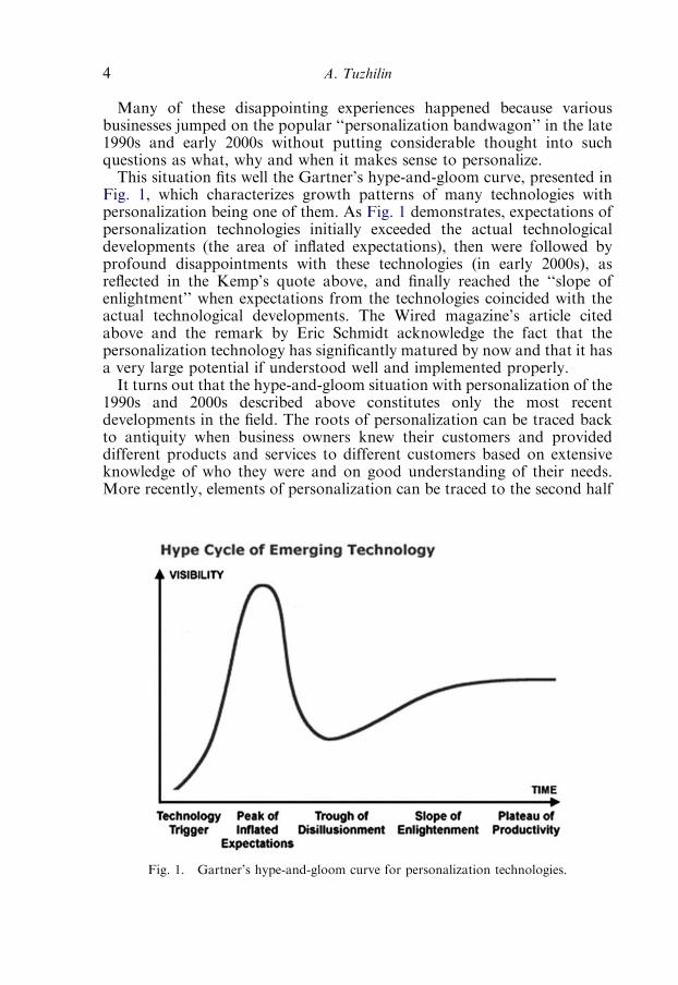
Many of these disappointing experiences happened because variousbusinesses jumped on the popular ‘‘personalization bandwagon’’ in the late1990s and early 2000s without putting considerable thought into suchquestions as what, why and when it makes sense to personalize.This situation fits well the Gartner’s hype-and-gloom curve, presented in
Fig. 1, which characterizes growth patterns of many technologies withpersonalization being one of them. As Fig. 1 demonstrates, expectations ofpersonalization technologies initially exceeded the actual technologicaldevelopments (the area of inflated expectations), then were followed byprofound disappointments with these technologies (in early 2000s), asreflected in the Kemp’s quote above, and finally reached the ‘‘slope ofenlightment’’ when expectations from the technologies coincided with theactual technological developments. The Wired magazine’s article citedabove and the remark by Eric Schmidt acknowledge the fact that thepersonalization technology has significantly matured by now and that it hasa very large potential if understood well and implemented properly.It turns out that the hype-and-gloom situation with personalization of the
1990s and 2000s described above constitutes only the most recentdevelopments in the field. The roots of personalization can be traced backto antiquity when business owners knew their customers and provideddifferent products and services to different customers based on extensiveknowledge of who they were and on good understanding of their needs.More recently, elements of personalization can be traced to the second half
Fig. 1. Gartner’s hype-and-gloom curve for personalization technologies.
A. Tuzhilin4
of the 19th century, when Montgomery Ward added some of the simplepersonalization features to their, otherwise, mass-produced catalogs (Ross,1992). However, all these early personalization activities were either doneon a small scale or were quite elementary.On a large scale, the roots of personalization can be traced to direct
marketing when the customer segmentation method based on the recency-frequency-monetary (RFM) model was developed by a catalog company todecide which customers should receive their catalog (Peterson et al., 1997).Also, the direct marketing company Metromail has developed the Selectionby Individual Families and Tracts (SIFT) system in mid-1960s thatsegmented the customers based on such attributes as telephone ownership,length of residence, head of household, gender and the type of dwelling tomake catalog shipping decisions. This approach was later refined in late1960s when customers were also segmented based on their ZIP codes. Thesesegmentation efforts were also combined with content customization whenTime magazine experimented with sending mass-produced letters in 1940sthat began with the salutation ‘‘Dear Mr. Smith . . . ’’ addressed to all theMr. Smith’s on the company’s mailing list (Reed, 1949). However, all theseearly-day personalization approaches were implemented ‘‘by hand’’ withoutusing Information Technologies.It was only in the mid-1960s, however, that direct marketers began using
IT to provide personalized services, such as producing computer-generatedletters that were customized to the needs of particular segments ofcustomers. As an early example of such computerized targeted marketing,Fingerhut targeted New York residents with personalized letters thatbegan, ‘‘Remember last January when temperatures in the state ofNew York dropped to a chilly �32 degrees?’’ (Peterson et al., 1997). Simi-larly, Burger King was one of the modern early adopters of personalizationwith ‘‘Have it your way’’ campaign launched in mid-1970s. However, it wasnot until 1980s that the areas of direct marketing and personalizationexperienced major advances due to the development of more powerfulcomputers, database technologies and more advanced data analysismethods (Peterson et al., 1997) and automated personalization became areality.Personalization was taken to the next level in the mid- to late-1990s with
the advancement of the Web technologies and various personalization toolshelping marketers interact with their customers on a 1-to-1 basis in realtime. As a result, a new wave of personalization companies has emerged,such as Broadvision, ATG, Blue Martini, e.Piphany, Kana, DoubleClick,Claria, ChoiceStream and several others. As an example, the PersonalWebplatform developed by Claria provides behavioral targeting of websitevisitors by ‘‘watching’’ their clicks and delivering personalized onlinecontent, such as targeted ads, news and RSS feeds, based on the analysis oftheir online activities. Claria achieves this behavioral targeting byrequesting online users to download and install the behavior-tracking
Ch. 1. Personalization: The State of the Art and Future Directions 5
software on their computers. Similarly, ChoiceStream software helpsYahoo, AOL, Columbia House, Blockbuster and other companies topersonalize home pages for their customers and thus deliver relevantcontent, products, search results and advertising to them. The benefitsderived from such personalized solutions should be balanced againstpossible problems of violating consumer privacy (Kobsa, 2007). Therefore,some of these personalization companies, including DoubleClick andClaria, had problems with consumer privacy advocates in the past.On the academic front, personalization has been explored in the
marketing community since the 1980s. For example, Surprenant andSolomon (1987) studied personalization of services and concluded thatpersonalization is a multidimensional construct that must be approachedcarefully in the context of service design since personalization does notnecessarily result in greater consumer satisfaction with the service offeringsin all the cases. The field of personalization was popularized by Peppers andRogers since the publication of their first book (Peppers and Rogers, 1993)on 1-to-1 marketing in 1993. Since that time, many publications appearedon personalization in computer science, information systems, marketing,management science and economics literature.In the computer science and information system literature, special issues
of the CACM (Communications of the ACM, 2000) and the ACM TOIT(Mobasher and Anand, 2007) journals were dedicated to personalizationtechnologies already, and another one (Mobasher and Tuzhilin, 2009) willbe published shortly. Some of the most recent reviews and surveys ofpersonalization include Adomavicius and Tuzhilin (2005a), Eirinaki andVazirgiannis (2003) and Pierrakos et al. (2003). The main topics inpersonalization studied by computer scientists include Web personalization(Eirinaki and Vazirgiannis, 2003; Mobasher et al., 2000; Mobasher et al.,2002; Mulvenna et al., 2000; Nasraoui, 2005; Pierrakos et al., 2003;Spiliopoulou, 2000; Srivastava et al., 2000; Yang and Padmanabhan, 2005),recommender systems (Adomavicius and Tuzhilin, 2005b; Hill et al., 1995;Pazzani, 1999; Resnick et al., 1994; Schafer et al., 2001; Shardanand andMaes, 1995), building user profiles and models (Adomavicius and Tuzhilin,2001a; Billsus and Pazzani, 2000; Cadez et al., 2001; Jiang and Tuzhilin,2006a,b; Manavoglu et al., 2003; Mobasher et al., 2002; Pazzani andBillsus, 1997), design and analysis of personalization systems (Adomaviciusand Tuzhilin, 2002; Adomavicius and Tuzhilin, 2005a; Eirinaki andVazirgiannis, 2003; Padmanabhan et al., 2001; Pierrakos et al., 2003; Wuet al., 2003) and studies of personalized searches (Qiu and Cho, 2006; Tsoiet al., 2006).1 Most of these areas have a vast body of literature and can be asubject of a separate survey. For example, the survey of recommender
1There are many papers published in each of these areas. The references cited above are either surveysor serve only as representative examples of some of this work demonstrating the scope of the efforts inthese areas; they do not provide exhaustive lists of citations in each of the areas.
A. Tuzhilin6

systems (Adomavicius and Tuzhilin, 2005b) cites over a 100 papers, and the2003 survey of Web personalization (Eirinaki and Vazirgiannis, 2003) cites40 papers on the corresponding topics, and these numbers grow rapidlyeach year.In the marketing literature, the early work on personalization (Surprenant
and Solomon, 1987) and (Peppers and Rogers, 1993), described above, wasfollowed by several authors studying such problems as targeted marketing(Chen and Iyer, 2002; Chen et al., 2001; Rossi et al., 1996), competitivepersonalized promotions (Shaffer and Zhang, 2002), recommender systems(Ansari et al., 2000; Haubl and Murray, 2003; Ying et al., 2006),customization (Ansari and Mela, 2003) and studies of effective strategiesof personalization services firms (Pancras and Sudhir, 2007).In the economics literature, there has been work done on studying
personalized pricing when companies charge different prices to differentcustomers or customer segments (Choudhary et al., 2005; Elmaghraby andKeskinocak, 2003; Jain and Kannan, 2002; Liu and Zhang, 2006; Ulph andVulkan, 2001). In the management science literature, the focus has been oninteractions between operations issues and personalized pricing (Elmaghrabyand Keskinocak, 2003) and also on the mass customization problems(Pine, 1999; Tseng and Jiao, 2001) and their limitations (Zipkin, 2001).Some of the management science and economics-based approaches toInternet-based product customization and pricing are described in Dewanet al. (2000). A review of the role of management science in research onpersonalization is presented in Murthi and Sarkar (2003).With all these advances in the academic research on personalization and
in developing personalized solutions in the industry, personalization ‘‘isback,’’ as is evidenced by the aforementioned quotes from the Wiredmagazine article and Eric Schmidt. In order to understand these sharpswings in perception about personalization, as described above, and graspgeneral developments in the field, we first review the basic concepts ofpersonalization, starting with its definition in Section 2. In Section 3, weexamine different types of personalization since, according to David Smith(2000), ‘‘there are myriad ways to get personal,’’ and we need to understandthem to have a good grasp of personalization. In Section 4, we discuss whenit makes sense to personalize. In Section 5, we present a personalizationprocess. In Section 6, we explain how different stages of the personalizationprocess can be integrated into one coherent system. Finally, we discussfuture research directions in personalization in Section 7.
2 Definition of personalization
Since personalization constitutes a rapidly developing field, there stillexist different points of view on what personalization is, as expressed by
Ch. 1. Personalization: The State of the Art and Future Directions 7

academics and practitioners. Some representative definitions of personali-zation proposed in the literature are
� ‘‘Personalization is the ability to provide content and services that aretailored to individuals based on knowledge about their preferences andbehavior’’ (Hagen, 1999).� ‘‘Personalization is the capability to customize communication basedon knowledge preferences and behaviors at the time of interaction’’(Dyche, 2002).� ‘‘Personalization is about building customer loyalty by building ameaningful 1-to-1 relationship; by understanding the needs of eachindividual and helping satisfy a goal that efficiently and knowledgeablyaddresses each individual’s need in a given context’’ (Riecken, 2000).� ‘‘Personalization involves the process of gathering user informationduring interaction with the user, which is then used to deliverappropriate content and services, tailor-made to the user’s needs’’(www.ariadne.ac.uk/issue28/personalization).� ‘‘Personalization is the ability of a company to recognize and treat itscustomers as individuals through personal messaging, targeted bannerads, special offers, . . . or other personal transactions’’ (Imhoff et al.,2001).� ‘‘Personalization is the combined use of technology and customerinformation to tailor electronic commerce interactions between abusiness and each individual customer. Using information eitherpreviously obtained or provided in real-time about the customer andother customers, the exchange between the parties is altered to fit thatcustomer’s stated needs so that the transaction requires less time and deli-vers a product best suited to that customer’’ (www.personalization.com—as it was defined on this website in early 2000s).
Although different, all these definitions identify several important pointsabout personalization. Collectively, they maintain that personalizationtailors certain offerings by providers to consumers based on certainknowledge about them, on the context in which these offerings are providedand with certain goal(s) in mind. Moreover, these personalized offeringsare delivered from providers to consumers through personalization enginesalong certain distribution channels based on the knowledge about theconsumers, the context and the personalization goals. Each of the italicizedwords above is important, and will be explained below.
1. Offerings. Personalized offerings can be of very different types. Someexamples of these offerings include
� Products, both ready-made that are selected for the particular consumer(such as books, CDs, vacation packages and other ready-madeproducts offered by a retailer) and manufactured in a custom-made
A. Tuzhilin8
fashion for a particular consumer (such as custom-made CDs andcustom-designed clothes and shoes).� Services, such as individualized subscriptions to concerts andpersonalized access to certain information services.� Communications. Personalized offerings can include a broad range ofmarketing and other types of communications, including targeted ads,promotions and personalized email.� Online content. Personalized content can be generated for an individualcustomer and delivered to him or her in the best possible manner. Thispersonalized content can include dynamically generated Web pages,new and modified links and insertion of various communicationsdescribed above into pre-generated Web pages.� Information searches. Depending on the past search history and onother personal characteristics of an online user, a search engine canreturn different search results or present them in a different order tocustomize them to the needs of a particular user (Qiu and Cho, 2006;Tsoi et al., 2006).� Dynamic prices. Different prices can be charged for different productsdepending on personal characteristics of the consumer (Choudharyet al., 2005).
These offerings constitute the marketing outputs of the personalizationprocess (Vesanen and Raulas, 2006).Given a particular type of offering, it is necessary to specify the universe
(or the space) of offerings O of that type and identify its structure. Forexample, in case of the personalized online content, it is necessary toidentify what kind of content can be delivered to the consumer, how‘‘granular’’ it is and what the structure of this content is. Similarly, in caseof personalized emails, it is necessary to specify what the structure of anemail message is, which parts of the message can be tailored and which arefixed, and what the ‘‘space’’ of all the email messages is. Similarly, in case ofpersonalized prices, it is important to know what the price ranges are andwhat the granularity of the price unit is if the prices are discrete.
2. Consumers can be considered either at the individual level or grouped intosegments depending on the particular type of personalization, the type oftargeting and personalization objectives. The former case fits into the 1-to-1paradigm (Peppers and Rogers, 1993), whereas the latter one into thesegmentation paradigm (Wedel and Kamakura, 2000).It is an interesting and important research question to determine which of
these two approaches is better and in which sense. The 1-to-1 approachbuilds truly personalized models of consumers but may suffer from nothaving enough data and the data being ‘‘noisy,’’ i.e., containing varioustypes of consumer biases, imperfect information, mistakes, etc. (Chen et al.,2001), whereas the segmentation approach has sufficient data but maysuffer from the problem of having heterogeneous populations of consumers
Ch. 1. Personalization: The State of the Art and Future Directions 9
within the segments. This question has been studied before by marketersand the results of this work are summarized in Wedel and Kamakura(2000). In the IS/CS literature, some solutions to this problem are describedin Jiang and Tuzhilin (2006a,b, 2007). Moreover, this problem will bediscussed further in Section 3.3.Note that some of the definitions of personalization presented above refer
to customers, while others to users and individuals. In the most generalsetting, personalization is applicable to a broad set of entities, includingcustomers, suppliers, partners, employees and other stakeholders in theorganization. In this chapter, we will collectively refer to these entities asconsumers by using the most general meaning of this term in the sensedescribed above.
3. Providers are the entities that provide personalized offerings, such ase-commerce websites, search engines and various offline outlets andorganizations.
4. Tailoring. Given the space O of all the possible offerings described aboveand a particular consumer or a segment of consumers c, which offering or aset of offerings should be selected from the space O in each particularsituation to customize the offering(s) to the needs of c according to thepersonalization goal(s) described below.How to deliver these customized offerings to individual consumers
constitutes one of the key questions of personalization. We will address thisquestion in Section 5 (Stage 3) when describing the ‘‘matchmaking’’ stage ofthe personalization process.
5. Knowledge about consumers. All the available information about theconsumer, including demographic, psychographic, browsing, purchasingand other transactional information, is collected, processed, transformed,analyzed and converted into actionable knowledge that is stored inconsumer profiles. This information is gathered from multiple sources.One of the crucial sources of this knowledge is the transactional informationabout interactions between the personalization system and the consumer,including purchasing transactions, browsing activities and various types ofinquiries and information gathering interactions. This knowledge obtainedfrom the collected data and stored in the consumer profiles is subsequentlyused to determine how to customize offerings to the consumers.The consumer profiles contain two types of knowledge. First, it has
factual knowledge about consumers containing demographic, transactionaland other crucial consumer information that is processed and aggregatedinto a collection of facts about the person, including various statistics aboutthe consumer’s behavior. Simple factual information about the consumercan be stored as a record in a relational database or as a consumer-centricdata warehouse (DW) (Kimball, 1996). More complicated factualinformation, such as the information about the social network of a person
A. Tuzhilin10
and his or her relationships and interactions with other consumers, mayrequire the use of taxonomies and ontologies and can be captured usingXML or special languages for defining ontologies (Staab and Studer, 2003),such as OWL (Antoniou and Harmelen, 2003). Second, the consumerprofile contains one or several data mining and statistical models capturingbehavior either of this particular consumer of the segment of similarconsumers to which the person belongs. These models are stored as a partof the consumer-centric modelbase (Liu and Tuzhilin, 2008). Together, thesetwo parts form the consumer profile that will be described in greater detailin Section 5.
6. Context. Tailoring of particular offering to the needs of the consumersdepends not only on the knowledge about the consumer, but also on thecontext in which this tailoring occurs. For example, when recommending amovie to the consumer, it is not only important to know his or her moviepreferences, but also the context in which these recommendations are made,such as with whom the person is going to see a movie, when and where. If aperson wants to see a movie with his girlfriend in a movie theater onSaturday night, then, perhaps, a different movie should be recommendedthan in the case if he wants to see it with his parents on Thursday evening athome on a VCR. Similarly, when a consumer shops for a gift, differentproducts should be offered to her in this context than when she shops forherself.
7. Goal(s) determine the purpose of personalization. Tailoring particularofferings to the consumers can have various objectives, including
� Maximizing consumer satisfaction with the provided offering and theoverall consumer experience with the provider.� Maximizing the Lifetime Value (LTV) (Dwyer, 1989) of the consumerthat determines the total discounted value of the person derivedover the entire lifespan of the consumer. This maximization is doneover a long-range time horizon rather than pursuing short-termsatisfaction.� Improving consumer retention and loyalty and decreasing churn. Forexample, the provider should tailor its offerings so that this tailoringwould maximize repeat visits of the consumer to the provider. The dualproblem is to minimize the churn rates, i.e., the rates at which thecurrent consumers abandon the provider.� Better anticipate consumers’ needs and, therefore, serve thembetter. One way to do this would be to design the personalizationengine so that it would maximize predictive performance of tailoredofferings, i.e., it would try to select the offerings that the consumerlikes.� Make interactions between providers and consumers efficient,satisfying and easier for both of them. For example, in case of Web
Ch. 1. Personalization: The State of the Art and Future Directions 11

personalization, this amounts to the improvement of the website designand helping visitors to find relevant information quickly andefficiently. Efficiency may also include saving consumer time. Forexample, a well-organized websites may help consumers to come in,efficiently buy product(s) and exist, thus saving precious time for theconsumer.� Maximize conversion rates whenever applicable, i.e., convert prospec-tive customers into buyers. For example, in case of Web personaliza-tion, this would amount to converting website visitors and browsersinto buyers.� Increase cross- and up-selling of provider’s offerings.
The goals listed above can be classified into marketing- and economics-oriented. In the former case, the goal is to understand and satisfy the needsof the consumers, sometimes even at the expense of the short-term financialperformance for the company, as is clearly demonstrated with the second(LTV) goal. For example, an online retailer may offer products and servicesto the consumer to satisfy his or her needs even if these offerings are notprofitable to the retailer in the short term. In the latter case, the goal is toimprove the short-term financial performance of the provider of thepersonalization service. As was extensively argued in the marketingliterature, all the marketing-oriented goals, eventually, contribute to thelong-term financial performance of the company (Kotler, 2003). Therefore,the difference between the marketing- and the economics-oriented goalsboils down to the long- vs. the sort-term performance of the company and,thus, both types of goals are based on the fundamental economic principles.Among the seven examples of personalization goals listed above, the first
five goals are marketing-oriented, whereas the last two are economics-oriented since their objectives are to increase the immediate financialperformance of the company. Finally, a personalization service providercan simultaneously pursue multiple goals, among which some can bemarketing- and others economics-oriented goals.
8. Personalization engine is a software system that delivers personalizedofferings from providers to consumers. It is responsible for providingcustomized offerings to the consumers according to the goals of thepersonalization system, such as the ones described above.
9. Distribution channel. Personalized offerings are delivered from theproducers to the consumers along one or several distribution channels, suchas a website, physical stores, email, etc. Selecting the right distributionchannel for a particular customized offering often constitutes an importantmarketing decision. Moreover, the same offering can be delivered alongmultiple distribution channels. Selecting the right mixture of channelscomplementing each other and maximizing the distribution effects
A. Tuzhilin12
constitutes the cross-channel optimization problem in marketing (IBMConsulting Services, 2006).If implemented properly, personalization can provide several important
advantages for the consumers and providers of personalized offeringsdepending on the choice of specific goals listed in item (7) above. Inparticular, it can improve consumer satisfaction with the offerings and theconsumer experience with the providers; it can make consumer interac-tions easier, more satisfying, efficient and less time consuming. It canimprove consumer loyalty, increase retention, decrease churn rates andthus can lead to higher LTVs of some of the consumers. Finally,well-designed economics-oriented personalization programs lead tohigher conversion and click-through rates and better up- and cross-sellingresults.Besides personalization, mass customization (Tseng and Jiao, 2001;
Zipkin, 2001) constitutes another popular concept in marketing andoperations management, which is sometimes used interchangeably withpersonalization in the popular press. Therefore, it is important todistinguish these two concepts to avoid possible confusion. According toTseng and Jiao (2001), mass customization is defined as ‘‘producing goodsand services to meet individual customer’s needs with near mass productionefficiency.’’ According to this definition, mass customization deals withefficient production of goods and services, including manufacturing ofcertain products according to specified customer needs and desires. It is alsoimportant to note that these needs and desires are usually explicitly specifiedby the customers in mass customization systems, such as specifying thebody parameters for manufacturing customized jeans, the feet parametersfor manufacturing customized shoes and computer configurations forcustomized PCs. In contrast to the case of mass customization, offerings areusually tailored to individual consumers without any significant productionprocesses in case of personalization. Also, in case of personalization, theknowledge about the needs and desires of consumers is usually implicitlylearned from multiple interactions with them rather than it being explicitlyspecified by the consumers in case of mass customization. For example, incase of customized websites, such as myYahoo!, the user specifies herinterests, and the website generates content according to the specifiedinterests of the user. This is in contrast to the personalized web page onAmazon, when Amazon observes the consumer purchases, implicitly learnsher preferences and desires from these purchases and personalizes her‘‘welcome’’ page according to this acquired knowledge. Therefore,personalization is about learning and responding to customer needs,whereas mass customization is about explicit specification of these needsby the customers and customizing offered products and services to theseneeds by tailoring production processes.In this section, we explained what personalization means. In the next
section, we describe different types of personalization.
Ch. 1. Personalization: The State of the Art and Future Directions 13

3 Types of personalization
Tailoring of personalized offerings by providers to consumers can comein many different forms and shapes, thus resulting in various types ofpersonalization. As David Smith put it, ‘‘there are myriad ways to getpersonal’’ (Smith, 2000). In this section, we describe different types ofpersonalization.
3.1 Provider- vs. consumer- vs. market-centric personalization
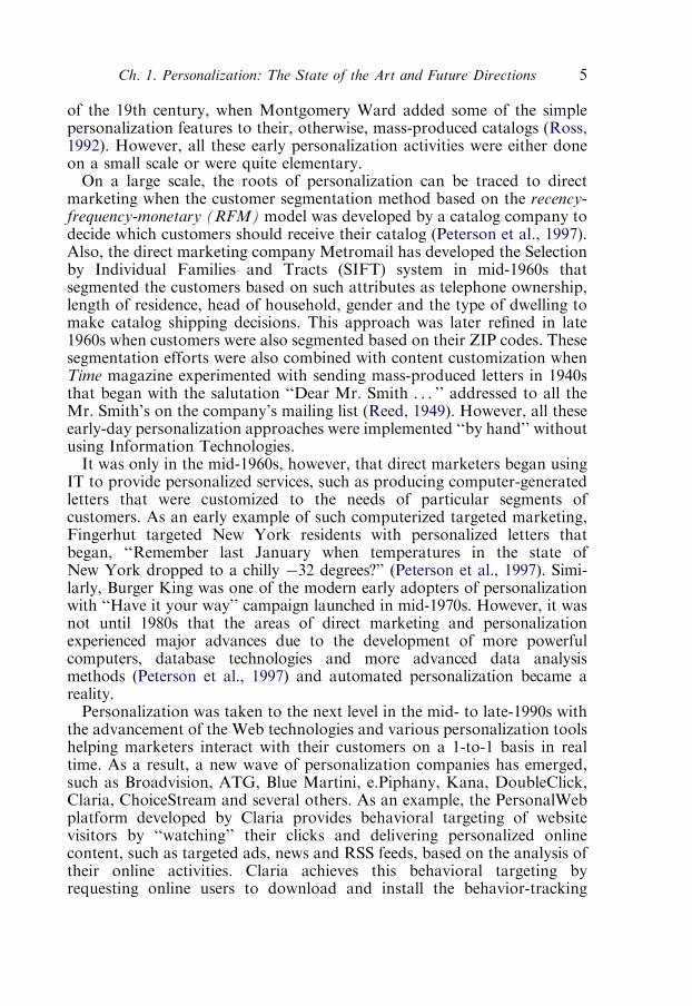
Personalized offerings can be delivered from providers to consumers bypersonalization engines in three ways, as presented in Fig. 2 (Adomaviciusand Tuzhilin, 2005a). In these diagrams, providers and consumers ofpersonalized offerings are denoted by white boxes, personalization enginesby gray boxes and the interactions between consumers and providers bysolid lines. Figure 2(a) presents the provider-centric personalizationapproach that assumes that each provider has its own personalizationengine that tailors the provider’s content to its consumers. This is the mostcommon approach to personalization, as popularized by Amazon.com,Netflix and the Pandora streaming music service. In this approach, there aretwo sets of goals for the personalization engines. On the one hand, theyshould provide the best marketing service to their customers and fulfillsome of the marketing-oriented goals presented in Section 2. On the otherhand, these provider-centric personalization services are designed toimprove financial performance of the providers of these services (e.g.,Amazon.com and Netflix), and therefore their behavior is driven by theeconomics-oriented goals listed in Section 2. Therefore, the challenge forthe provider-centric approaches to personalization is to strike a balancebetween the two sets of goals by keeping the customers happy with tailoredofferings and making personalization solutions financially viable for theprovider.
Consumers Providers Providers Providers
(a) Provider-centric (b) Consumer-centric (c) Market-centric
Consumers Consumers
Fig. 2. Classification of personalization approaches.
A. Tuzhilin14
The second approach, presented in Fig. 2(b), is the consumer-centricapproach, which assumes that each consumer has its own personalizationengine (or agent) that ‘‘understands’’ this particular consumer and providespersonalization services across several providers based on this knowledge.This type of consumer-centric personalization delivered across a broadrange of providers and offerings is called an e-Butler service (Adomaviciusand Tuzhilin, 2002) and is popularized by the PersonalWeb service fromClaria (www.claria.com). The goals of a consumer-centric personalizationservice are limited exclusively to the needs of the consumer and shouldpursue only the consumer-centric objectives listed in Section 2, such asanticipating consumer needs and making interactions with a website moreefficient and satisfying for the consumer. The problem with this approachlies in developing personalization service of such quality and value to theconsumers that they would be willing to pay for it. This would removedependency on advertising and other sources of revenues coming from theproviders of personalized services, which would go against the philosophyof the purely consumer-centric service.The third approach, presented in Fig. 2(c), is the market-centric approach
that provides personalization services for a marketplace in a certainindustry or sector. In this case, the personalization engine performs the roleof an infomediary by knowing the needs of the consumers and theproviders’ offerings and trying to match the two parties in the best waysaccording to their internal goals. Personalized portals customizing theservices offered by its corporate partners to the individual needs of theircustomers would be an example of this market-centric approach.
3.2 Types of personalized offerings
Types of personalization methods can vary very significantly dependingon the type of offering provided by the personalization application. Forexample, methods for determining personalized searches (Qiu and Cho,2006) differ significantly from the methods for determining personalizedpricing (Choudhary et al., 2005), which also differ significantly from themethods for delivering personalized content to the Web pages (Sheth et al.,2002) and personalized recommendations for useful products (Adomaviciusand Tuzhilin, 2005b).In Section 2, we identified various types of offerings including
� Products and services,� Communications, including targeted ads, promotions and personalizedemail,� Online content, including dynamically generated Web pages and links,� Information searches,� Dynamic prices.
Ch. 1. Personalization: The State of the Art and Future Directions 15
One of the defining factors responsible for differences in methods ofdelivering various types of personalized offerings is the structure andcomplexity of the offerings space O that can vary quite significantly acrossthe types of offerings listed above. For example, in case of dynamic prices,the structure of the offering space O is relatively simple (e.g., discrete orcontinuous variable within a certain range), whereas in case of onlinecontent tailoring it can be very large and complex depending on thegranularity of the web content and how the content is structured on the webpages of a particular personalization application. Another defining factor isconceptually different methods for delivering various types of targetedofferings. For example, how to specify dynamic prices depends on theunderlying economic theories, whereas providing personalized recommen-dations depends on the underlying data mining and other recommendationmethods discussed in Section 5. Similarly, methods of deliveringpersonalized searches depend on underlying information retrieval and websearch theories.A particular application can also deal with a mixture of various types of
offerings described above, which can result in a combination of differentpersonalization methods. For example, if an online retailer decides to adddynamic prices to the already developed personalized product offerings(i.e., customer X receives a recommendation for book Y at a personalizedprice Z), then this means combining personalized recommendationmethods, such as the ones discussed in Section 5, with personalized pricingmethods. Alternatively, a search engine may deliver personalized searchresults and personalized search-related ads targeted to individuals that arebased not only on the search keywords specified by the consumer, but alsoon the personal characteristics of the consumer, as defined in his or herprofile, such as the past search history, geographic location anddemographic data in case it is available.
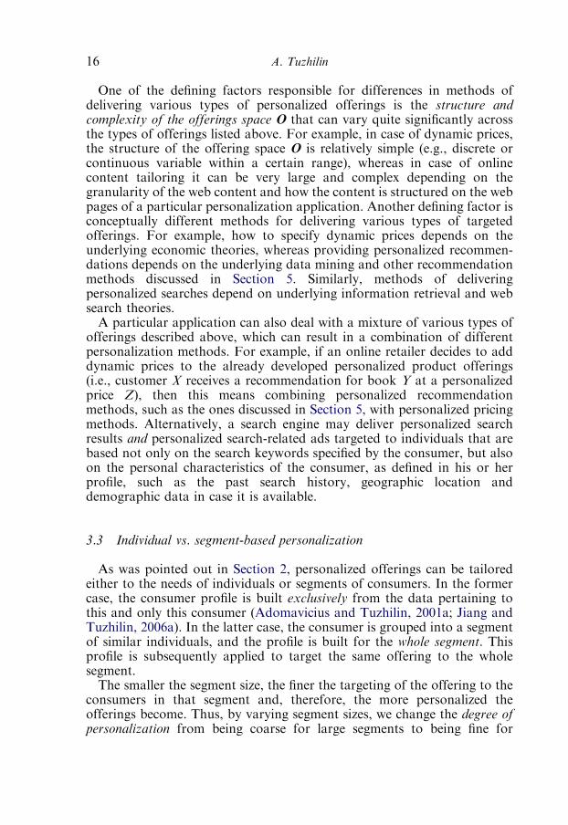
3.3 Individual vs. segment-based personalization
As was pointed out in Section 2, personalized offerings can be tailoredeither to the needs of individuals or segments of consumers. In the formercase, the consumer profile is built exclusively from the data pertaining tothis and only this consumer (Adomavicius and Tuzhilin, 2001a; Jiang andTuzhilin, 2006a). In the latter case, the consumer is grouped into a segmentof similar individuals, and the profile is built for the whole segment. Thisprofile is subsequently applied to target the same offering to the wholesegment.The smaller the segment size, the finer the targeting of the offering to the
consumers in that segment and, therefore, the more personalized theofferings become. Thus, by varying segment sizes, we change the degree ofpersonalization from being coarse for large segments to being fine for
A. Tuzhilin16

smaller segments. In the limit, complete personalization is reached forthe 1-to-1 marketing when the segment size is always one.Although strongly advocated in the popular press (Peppers and Rogers,
1993; Peppers and Rogers, 2004), it is not clear that targeting personalizedofferings to individual consumers will always be better than for segments ofconsumers because of the tradeoff between sparsity of data for individualconsumers and heterogeneity of consumers within segments: individualconsumer profiles may suffer from sparse data resulting in high variance ofperformance measures of individual consumer models, whereas aggregateprofiles of consumer segments suffer from high levels of customerheterogeneity, resulting in high performance biases. Depending on whicheffect dominates the other, it is possible that individualized personalizationmodels outperform the segmented or aggregated models, and vice versa.The tradeoff between these two approaches has been studied in Jiang and
Tuzhilin (2006a), where performance of individual, aggregate andsegmented models of consumer behavior was compared empirically acrossa broad spectrum of experimental settings. It was shown that for the highlytransacting consumers or poor segmentation techniques, individual-levelconsumer models outperform segmentation models of consumer behavior.These results reaffirm the anecdotal evidence about the advantages ofpersonalization and the 1-to-1 marketing stipulated in the popular press(Peppers and Rogers, 1993; Peppers and Rogers, 2004). However, theexperiments reported in Jiang and Tuzhilin (2006a) also show thatsegmentation models, taken at the best granularity level(s) and generatedusing effective clustering methods, dominate individual-level consumermodels when modeling consumers with little transactional data. Moreover,this best granularity level is significantly skewed towards the 1-to-1 case andis usually achieved at the finest segmentation levels. This finding providesadditional support for the case of micro-segmentation (Kotler, 2003;McDonnell, 2001)—when consumer segmentation is done at a highlygranular level.In conclusion, determining the right segment sizes and the optimal degree
of personalization constitutes an important decision in personalizationapplications and involves the tradeoff between heterogeneity of consumerbehavior in segmented models vs. sparsity of data for small segment sizesand individual models.
3.4 Smart vs. trivial personalization
Some personalization systems provide only superficial solutions, includ-ing presenting trivial content for the consumers, such as greeting them byname or recommending a book similar to the one the person has boughtrecently. As another example, a popular website personalization.com (or itsalias personalizationmall.com) provides personalized engravings on various
Ch. 1. Personalization: The State of the Art and Future Directions 17

items ranging from children’s backpacks to personalized beer mugs. Theseexamples constitute cases of trivial (Hagen, 1999) [shallow or cosmetic(Gilmore and Pine, 1997)] personalization.In contrast to this, if offerings are actively tailored to individuals based
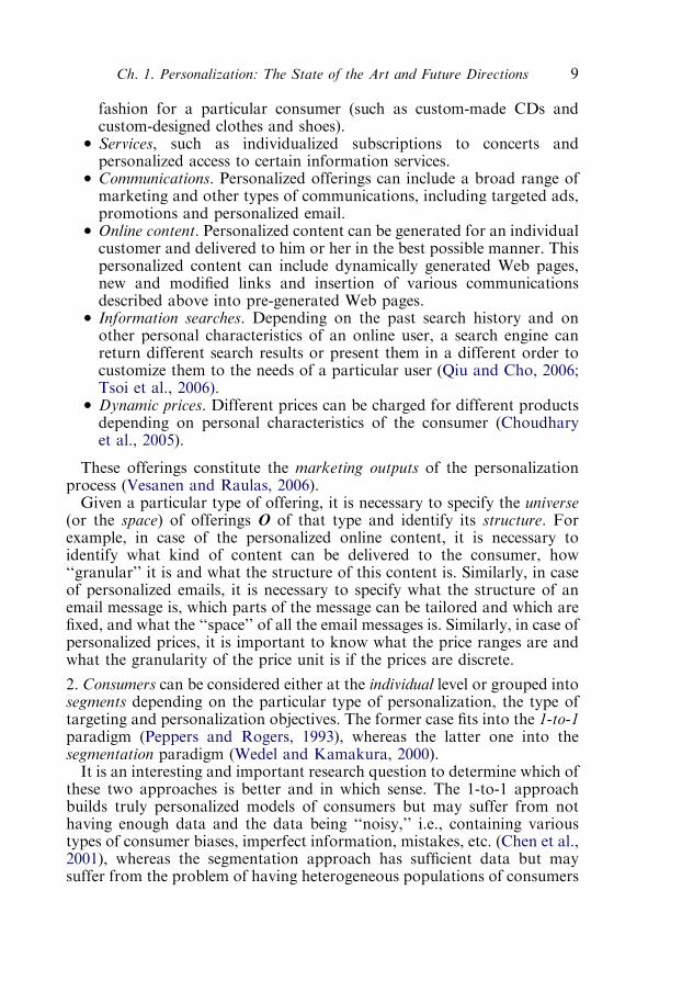
on rich knowledge about their preferences and behavior, then thisconstitutes smart (or deep) personalization (Hagen, 1999). Continuing thiscategorization further, Paul Hagen classifies personalization applicationsinto the following four categories, described with the 2� 2 matrix shown inFig. 3 (Hagen, 1999).According to Fig. 3 and Hagen (1999), one classification dimension
constitutes consumer profiles that are classified into rich vs. poor. Richprofiles contain comprehensive information about consumers and theirbehavior of the type described in Section 2 and further explained in Section5. Poor profiles capture only partial and trivial information aboutconsumers, such as their names and basic preferences. The seconddimension of the 2� 2 matrix in Fig. 3 constitutes tailoring (customization)of the offerings. According to Hagen (1999), the offerings can be tailoredeither reactively or proactively. Reactive tailoring takes already existingknowledge about consumers’ preferences and ‘‘parrots’’ these preferencesback to them without producing any new insights about potentially newand interesting offerings. In contrast, the proactive tailoring takesconsumer preferences stored in consumer profiles and generates new usefulofferings by using innovative matchmaking methods to be described inSection 5.Using these two dimensions, Hagen (1999) classifies personalization
applications into
� Trivial personalizers: These applications have poor profiles and providereactive targeting. For example, a company can ask many relevantquestions about consumer preferences, but would not use thisknowledge about them to build rich profiles of the customers anddeliver truly personalized and relevant content. Instead, the companyinsults its customers by ignoring their inputs and delivering irrelevantmarketing messages or doing cosmetic personalization, such asgreeting the customers by name.� Lazy personalizers: These applications build rich profiles, but do onlyreactive targeting. For example, an online drugstore can have rich
Rich profile Lazy
personalizers Smart
personalizers
Poor profile Trivial
personalizersOvereager
personalizers
Reactive tailoring Proactive tailoring
Fig. 3. Classification of personalization applications (Hagen, 1999).
A. Tuzhilin18

information about customer’s allergies, but miss or even ignore thisinformation when recommending certain drugs to patients. This canlead to recommending drugs causing allergies in patients, although theallergies information is contained in the patients’ profiles.� Overeager personalizers: These applications have poor profiles butmake proactive targeting of its offerings. This can often lead to poorresults because of the limited information about consumers and faultyassumptions about their preferences. Examples of these types ofapplications include recommending books similar to the ones theconsumer bought recently and various types of baby products to awoman who recently had a miscarriage.� Smart personalizers: These applications use rich profiles and provideproactive targeting of the offerings. For example, an online gardeningwebsite may warn a customer that the plant she just bought would notgrow well in the climate of the region where the customer lives. Inaddition, the website would recommend alternative plants based on thecustomers’ preferences and past purchases that would fit better theclimate where the customer lives.
On the basis of this classification, Hagen (1999), obviously, argues for theneed to develop smart personalization applications by building rich profilesof consumers and actively tailoring personalized offerings to them. At theheart of smart personalization lie two problems (a) how to build richprofiles of consumers and (b) how to match the targeted offerings to theseprofiles well. Solutions to these two problems will be discussed further inSection 5.
3.5 Intrusive vs. non-intrusive personalization
Tailored offerings can be delivered to the consumer in an automatedmanner without distracting her with questions and requests for informationand preferences. Alternatively the personalization engine can ask theconsumer various questions in order to provide better offerings. Forexample, Amazon.com, Netflix and other similar systems that recommendvarious products and services to individual consumers ask these con-sumers for some initial set of ratings of the products and services beforeproviding recommendations regarding them. Also, when a multidimen-sional recommender system wants to provide a recommendation in aspecific context, such as recommending a movie to a person who wants tosee it with his girlfriend on Saturday night in a movie theater, the systemwould first ask (a) when he wants to see the movie, (b) where and (c) withwhom before providing a specific recommendation (Adomavicius et al.,2005).Such personalization systems are intrusive in the sense that they keep
asking consumers questions before delivering personalized offerings to
Ch. 1. Personalization: The State of the Art and Future Directions 19

them, and the levels of consumer involvement can be very significant insome cases. Alternatively, personalization systems may not ask consumersexplicit questions, but non-intrusively learn consumer preferences fromvarious automated interactions with them. For example, the amount oftime a consumer spends reading a newsgroup article can serve as a proxy ofhow much the consumer is interested in this article. Clearly, non-intrusivepersonalization systems are preferable from the consumer point of view, butthey may provide less accurate recommendations. Studying the tradeoffsbetween intrusive and non-intrusive personalization systems and determin-ing optimal levels of intrusiveness in various personalization applicationsconstitutes an interesting and important research problem.This problem has already been studied by several researchers in the
context of recommender systems. In particular, Oard and Kim (1998)described several ways of obtaining implicit feedback for recommendersystems. The methods of minimizing the number of intrusive questions forobtaining user ratings in recommender systems have also been studied inPennock et al. (2000), Rashid et al. (2002), Boutilier et al. (2003),Montgomery and Srinivasan (2003) and Yu et al. (2004).
3.6 Static vs. dynamic personalization
Personalization applications can be classified in terms of who can selectand deliver the offerings and how this is done. On the one hand, theofferings can be selected and delivered dynamically by the personalizationsystem. For example, the system may be monitoring the activities ofthe consumer and the environment and dynamically deciding to changethe content of the web pages for the consumer based on her activitiesand the changes in the environment. One promising type of dynamicpersonalization constitutes ubiquitous personalization based on mobilelocation-based services (LBS) (Rao and Minakakis, 2003) that deployvarious types of wireless technologies that identify the location and othertypes of contextual information, such as the current time, the consumerschedule and the purpose of the trip, in order to provide dynamicpersonalized services to the consumer based on this contextual informationand the consumer profile. Examples of these LBS including suggestions ofvarious shops, restaurants, entertainment events and other points of interestin the geographical and temporal vicinities of the consumer.On the other hand, the offerings delivered to the consumer can be selected
either by the consumer herself or by the system administrator who hadselected a fixed set of business rules governing the delivery of the offeringsto specific segments of the consumers. In this case, this selection was donestatically and can be changed only by the consumer or the systemadministrator depending on the case.
A. Tuzhilin20
Obviously, the dynamic selection of offerings is more flexible and is morepreferred than the static selection process. On the other hand, it should bedone in a smart way, as described in Section 3.4 above, to avoid thesubstandard performance of the personalization system.In summary, we discussed various types of personalization in this section,
following the dictum of David Smith that ‘‘there are myriad ways to getpersonal’’ (Smith, 2000). Therefore, specific types of personalizationapproaches need to be selected carefully depending on the particularpersonalization application at hand and on the goals that this applicationtries to accomplish, such as the ones described in Section 2.
4 When does it pay to personalize?
One of the reasons why personalization has its share of successes anddisappointments is that it does not always make sense to personalize bothfor the technical and economic reasons. One of such technical reasons isthat provision of personalized offerings can lead to questionable outcomesthat do not benefit, or even worse, insult the consumer. For example, anonline maternity store can start recommending various types of babyproducts to a woman who has bought maternity clothes for herself a fewmonths ago without realizing that she had recently had a miscarriage. Oneof the fundamental assumptions in personalization is that of the stability ofconsumer preferences and the assumption that the past consumer activitiescan be used to predict their possible future preferences and actions. As theprevious example clearly demonstrates, this assumption does not hold insome cases. In those cases, the dangers of personalization and the risks offalling into the de-personalization trap (to be discussed in Section 5) mayoverweight the potential benefits of personalization, thus making itimpractical.On the economic side, proponents of personalization first need to build a
strong business case before launching a personalization project. At the mostgeneral level, personalization should be done when the benefits derivedfrom a personalization project exceed its costs for both providers andconsumers of personalized offerings. Otherwise, one of the parties willrefuse to participate in the personalization project. In the rest of thissection, we examine the costs vs. benefits tradeoff for both providers andconsumers of personalized offerings.
Consumers. From the consumers’ perspective, the benefits of personaliza-tion constitute more relevant offerings delivered by the providers at themost opportune moments. One problem with these types of benefits is thatit is hard to measure their effects, as will be discussed in Section 5. The costsof personalization consist of two parts for the consumers: direct andindirect. The direct costs are subscription costs paid by the consumers. For
Ch. 1. Personalization: The State of the Art and Future Directions 21

the provider-centric personalization, personalization services are usuallyprovided for free and, therefore, the direct costs for the consumers areusually zero. In case of the consumer-centric personalization, consumersshould pay for these services, as discussed in Section 3.1, and these feesconstitute the direct costs for the consumers. Indirect costs to theconsumers include time and cognitive efforts of installing and configuringpersonalization services, and the privacy and security issues associated withthese services. As a part of the subscription, the consumers should providecertain personal information to the personalization service providers, andthere are always some risks that this personal information can be misusedby the providers. As in the case of benefits, these indirect costs are also hardto measure.
Providers. For the providers, the key question is whether or not they shouldcustomize their offerings and if yes, then to what degree and scope. Thedecision to personalize its offerings or not depends on the tradeoff betweenthe personalization costs vs. the benefits derived by the providers frompersonalized offerings to the consumers. We will now examine these costsand benefits.Customization does not come for free since it requires additional costs to
customize offerings in most of the cases, especially in the case of customizedproducts that need to be manufactured. Also, the more personalized anoffering is, the more customization is usually required. For example, onematter is to make a certain type of shoe in 20 different varieties dependingon the color, foot size and width, and a completely different and moreexpensive proposition is to manufacture a personal pair of shoes for aspecific customer. In general, the more customized an offering is and thesmaller the targeted segment, the more costly the manufacturing processbecomes. In the limit, manufacturing for the segment of one is the mostexpensive, and it requires stronger business justification to adopt this option(Zipkin, 2001). One interesting research question is whether firms shouldcustomize their products based on one or multiple attributes and whetherdifferent firms should select the same or different attributes for customiza-tion purposes. In Syam et al. (2005), it is shown that it is better for the firmsto select only one and the same attribute as a basis for customization. Thisproblem was further explored in Ghose and Huang (2007). Moreover, it isalso important to know how customization of products and prices affecteach other. In Ghose and Huang (2006), it is shown that if the fixed costs ofpersonalization are low, firms are always better off personalizing bothprices and products. Shaffer and Zhang (2002) also show that similar effectscan arise if firms are asymmetric in market share.As for the consumers, personalization costs for the providers consist of
direct and indirect costs. The direct costs are associated with extra effortsrequired to customize personalized offerings, whereas indirect costs areassociated with the potential problems pertaining to providing personalized
A. Tuzhilin22
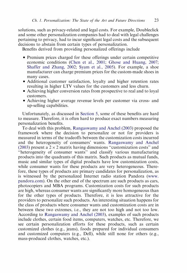
solutions, such as privacy-related and legal costs. For example, Doubleclickand some other personalization companies had to deal with legal challengespertaining to privacy, had to incur significant legal costs and the subsequentdecisions to abstain from certain types of personalization.Benefits derived from providing personalized offerings include
� Premium prices charged for these offerings under certain competitiveeconomic conditions (Chen et al., 2001; Ghose and Huang, 2007;Shaffer and Zhang, 2002; Syam et al., 2005). For example, a shoemanufacturer can charge premium prices for the custom-made shoes inmany cases.� Additional customer satisfaction, loyalty and higher retention ratesresulting in higher LTV values for the customers and less churn.� Achieving higher conversion rates from prospective to real and to loyalcustomers.� Achieving higher average revenue levels per customer via cross- andup-selling capabilities.
Unfortunately, as discussed in Section 5, some of these benefits are hardto measure. Therefore, it is often hard to produce exact numbers measuringpersonalization benefits.To deal with this problem, Rangaswamy and Anchel (2003) proposed the
framework where the decision to personalize or not for providers ismeasured in terms of the tradeoffs between the customization costs incurredand the heterogeneity of consumers’ wants. Rangaswamy and Anchel(2003) present a 2� 2 matrix having dimensions ‘‘customization costs’’ and‘‘heterogeneity of consumer wants’’ and classify various manufacturingproducts into the quadrants of this matrix. Such products as mutual funds,music and similar types of digital products have low customization costs,while consumer wants for these products are very heterogeneous. There-fore, these types of products are primary candidates for personalization, asis witnessed by the personalized Internet radio station Pandora (www.pandora.com). On the other end of the spectrum are such products as cars,photocopiers and MBA programs. Customization costs for such productsare high, whereas consumer wants are significantly more homogeneous thanfor the other types of products. Therefore, it is less attractive for theproviders to personalize such products. An interesting situation happens forthe class of products where consumer wants and customization costs are inbetween these two extremes, i.e., they are not too high and not too low.According to Rangaswamy and Anchel (2003), examples of such productsinclude clothes, certain food items, computers, watches, etc. Therefore, wesee certain personalization efforts for these products, such as certaincustomized clothes (e.g., jeans), foods prepared for individual consumersand customized computers (e.g., Dell), while still none for others (e.g.,mass-produced clothes, watches, etc.).
Ch. 1. Personalization: The State of the Art and Future Directions 23

In summary, when the benefits of personalization exceed its costs for bothproviders and consumers of personalized offerings, only then it makesbusiness sense to personalize, which happens only for certain types ofofferings and usually on a case-by-case basis. Moreover, it is difficult tomeasure the costs and benefits of personalization in many cases. Therefore,personalization decisions are often hard to make in real business settings,and they require careful cost-benefit analysis and evaluation.
5 Personalization process
As was argued by Adomavicius and Tuzhilin (2001b), personalizationshould be considered as an iterative process consisting of several stages thatare integrated together into one tight system. In particular, Adomaviciusand Tuzhilin (2001b) proposed the following five stages: (a) collectingcustomer data, (b) building customer profiles using this data,(c) matchmaking customized offerings to specific customer profiles todetermine the most relevant offerings to individual customers, (d) deliveryand presentation of customized information and offerings through the mostrelevant channels, at the most appropriate times and in the mostappropriate form and (e) measuring customer responses to the deliveredofferings. Moreover, Adomavicius and Tuzhilin (2001b) argued for thenecessity of a feedback loop mechanism that takes customers’ responses tothe current personalization solution, transfers appropriate information tothe earlier stages of the personalization process, and adjusts, improves andcorrects various activities in these earlier stages that cause poor responsesfrom the customers.This approach of viewing personalization as a process was further
developed by Murthi and Sarkar (2003), who partitioned the personaliza-tion process into the following three stages: (a) learning customerpreferences, (b) matching offerings to customers’ preferences and(c) evaluation of the learning and matching processes. Murthi and Sarkar(2003) also placed personalization within the firm’s overall Value Netframework and connected it to the general business strategy of the firm.Subsequently, Adomavicius and Tuzhilin (2005a) extended and refined
the previous approaches by proposing the Understand–Deliver–Measure(UDM) framework, according to which the personalization process isdefined in terms of the UDM cycle consisting of the following stages asshown in Fig. 4:
� Understand consumers by collecting comprehensive information aboutthem and converting it into actionable knowledge stored in consumerprofiles. The output of this stage is a consumer-centric DW (Kimball,1996) and the consumer-centric modelbase (Liu and Tuzhilin, 2008).The consumer-centric DW stores factual profiles of each consumer.
A. Tuzhilin24

The consumer-centric modelbase stores data mining and statisticalmodels describing behavior of individual consumers. Collectively,factual profile and the collection of data mining models of theconsumer form the consumer profile.� Deliver customized offering based on the knowledge about eachconsumer C, as stored in the consumer profiles, and on the informationabout the space of offerings O. The personalization engine should findthe customized offerings from the space O that are the most relevant toeach consumer C within the specified context and deliver them to C inthe best possible manner, including at the most appropriate time(s),through the most appropriate channels and in the most appropriateform. These customized offerings constitute marketing outputs of thepersonalization process.� Measure personalization impact by determining how much theconsumer is satisfied with the marketing outputs (in the form ofdelivered personalized offerings). It provides information that canenhance our understanding about consumers or point out thedeficiencies of the methods for personalized delivery. Therefore, thisadditional information serves as a feedback for possible improvementsto each of the other components of personalization process. Thisfeedback information completes one cycle of the personalizationprocess, and sets the stage for the next cycle where improvedpersonalization techniques can make better personalization decisions.
More recently, Vesanen and Raulas (2006) presented an alternativeapproach to describing the personalization process that consists of interaction,
Measuring Personalization Impact
Data Collection
Building Consumer Profiles
Matchmaking
Delivery and Presentation
Measure Impact of
Personalization
Deliver Customized Offerings
Understand the Consumer
Adjusting Personalization Strategy
Feed
back
loop
Fig. 4. Personalization process.
Ch. 1. Personalization: The State of the Art and Future Directions 25

processing, customization and delivery stages. In addition, Vesanen andRaulas (2006) explicitly introduced four objects into its framework:customers, customer data, customer profiles and marketing outputs, andshowed how the aforementioned four stages are connected to these fourobjects. In particular, they described how customer data is obtained fromthe customers via interactions with them and from the external sources,then how it is preprocessed into the customer profiles, and then howmarketing outputs are customized based on the profiling information.Vesanen and Raulas (2006) also argue for the importance of integratingvarious personalization stages and describe possible problems arising fromimproper integration of various stages of the personalization process andthe existence of the ‘‘discontinuity points.’’ Finally, Vesanen and Raulas(2006) present a case study describing how the described personalizationprocess was implemented in a direct marketing company.Although each of the described approaches covers different aspects of the
personalization process, we will follow below the modified UDM modelfrom Adomavicius and Tuzhilin (2005a) that is schematically described inFig. 4, because we believe that this modified UDM model covers all theaspects of the personalization process. For example, the four personaliza-tion stages presented in Vesanen and Raulas (2006) are closely related to thesix stages of the personalization process presented in Fig. 4.The UDM framework described above constitutes the high-level
conceptual description of the personalization process. The technicalimplementation of the UDM framework consists of the following sixstages (Adomavicius and Tuzhilin, 2005a) presented in Fig. 4:
Stage 1: Data Collection. The personalization process begins with collectingdata across different channels of interaction between consumers andproviders (e.g., Web, phone, direct mail and other channels) and fromvarious other external data sources with the objective of obtaining the mostcomprehensive ‘‘picture’’ of a consumer. Examples of the ‘‘interactions’’data includes browsing, searching and purchasing data on the Web, directmail, phone and email interactions data, and various demographic andpsychographic data collected through filling various online and offlineforms and surveys. Examples of external data can be economic, industry-specific, geographic and census data either purchased or obtained from theexternal sources through means other than direct interactions with theconsumer.
Stage 2: Building Customer Profiles. Once the data is collected, one of thekey issues in developing personalization applications is integrating this dataand constructing accurate and comprehensive consumer profiles based on thecollected data. Many personalization systems represent consumer profiles interms of a collection of facts about the consumer. These facts may includeconsumer’s demographics, such as name, gender, date of birth and address.The facts can also be derived from the past transactions of a consumer,
A. Tuzhilin26
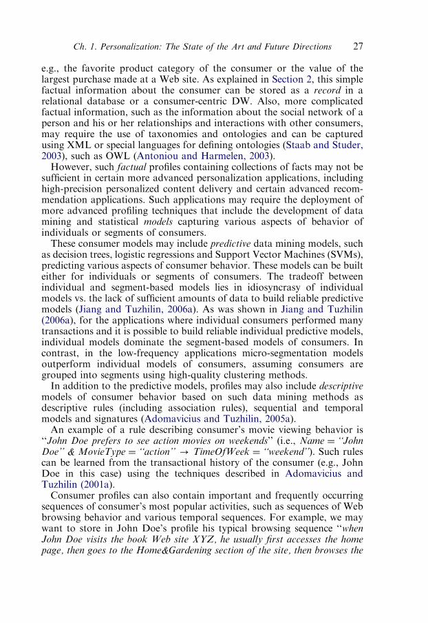
e.g., the favorite product category of the consumer or the value of thelargest purchase made at a Web site. As explained in Section 2, this simplefactual information about the consumer can be stored as a record in arelational database or a consumer-centric DW. Also, more complicatedfactual information, such as the information about the social network of aperson and his or her relationships and interactions with other consumers,may require the use of taxonomies and ontologies and can be capturedusing XML or special languages for defining ontologies (Staab and Studer,2003), such as OWL (Antoniou and Harmelen, 2003).However, such factual profiles containing collections of facts may not be
sufficient in certain more advanced personalization applications, includinghigh-precision personalized content delivery and certain advanced recom-mendation applications. Such applications may require the deployment ofmore advanced profiling techniques that include the development of datamining and statistical models capturing various aspects of behavior ofindividuals or segments of consumers.These consumer models may include predictive data mining models, such
as decision trees, logistic regressions and Support Vector Machines (SVMs),predicting various aspects of consumer behavior. These models can be builteither for individuals or segments of consumers. The tradeoff betweenindividual and segment-based models lies in idiosyncrasy of individualmodels vs. the lack of sufficient amounts of data to build reliable predictivemodels (Jiang and Tuzhilin, 2006a). As was shown in Jiang and Tuzhilin(2006a), for the applications where individual consumers performed manytransactions and it is possible to build reliable individual predictive models,individual models dominate the segment-based models of consumers. Incontrast, in the low-frequency applications micro-segmentation modelsoutperform individual models of consumers, assuming consumers aregrouped into segments using high-quality clustering methods.In addition to the predictive models, profiles may also include descriptive
models of consumer behavior based on such data mining methods asdescriptive rules (including association rules), sequential and temporalmodels and signatures (Adomavicius and Tuzhilin, 2005a).An example of a rule describing consumer’s movie viewing behavior is
‘‘John Doe prefers to see action movies on weekends’’ (i.e., Name ¼ ‘‘JohnDoe’’ & MovieType ¼ ‘‘action’’ - TimeOfWeek ¼ ‘‘weekend’’). Such rulescan be learned from the transactional history of the consumer (e.g., JohnDoe in this case) using the techniques described in Adomavicius andTuzhilin (2001a).Consumer profiles can also contain important and frequently occurring
sequences of consumer’s most popular activities, such as sequences of Webbrowsing behavior and various temporal sequences. For example, we maywant to store in John Doe’s profile his typical browsing sequence ‘‘whenJohn Doe visits the book Web site XYZ, he usually first accesses the homepage, then goes to the Home&Gardening section of the site, then browses the
Ch. 1. Personalization: The State of the Art and Future Directions 27

Gardening section and then leaves the Web site’’ (i.e., XYZ: StartPage -Home&Gardening - Gardening - Exit). Such sequences can be learnedfrom the transactional histories of consumers using frequent episodes andother sequence learning methods (Hand et al., 2001).Finally, consumer profiles can also contain signatures of consumer
behavior (Cortes et al., 2000) that are the data structures used to capturethe evolving behavior learned from large data streams of simpletransactions (Cortes et al., 2000). For example, ‘‘top 5 most frequentlybrowsed product categories over the last 30 days’’ would be an example of asignature that could be stored in individual consumer profiles in a Webstore application.In summary, besides factual information about consumers, their profiles
can also contain various data mining and statistical models describingconsumer behavior, such as predictive, descriptive rule-based, sequential,temporal models and signatures.All this consumer profiling information can be stored in two types of
repositories
� Consumer-centric DW (Kimball, 1996), where each consumer has aunique record or a taxonomy containing demographic and otherfactual information describing his or her activities.� Consumer-centric modelbase (Liu and Tuzhilin, 2008) containing oneor several models describing different aspects of behavior of aconsumer. As explained before, a model can be unique for a consumeror a segment of consumers, and can be organized and stored in themodelbase in several different ways (Liu and Tuzhilin, 2008).However, each consumer should have a list of all the models describingbehavior of that consumer that is easily accessible and managed.Collectively, the set of all the models of all the consumers forms amodelbase, and it is organized and managed according to theprinciples described in Liu and Tuzhilin (2008).
Stage 3: Matchmaking. Once the consumer profiles are constructed,personalization systems must be able to match customized offerings toindividuals or segments of consumers within a certain context, such asshopping for yourself vs. for a friend, based on the consumer profilinginformation obtained in Stage 2 and on the information about the space ofofferings O. The matchmaking process should find customized offeringsfrom the space O that are the most relevant to each consumer C within thespecified context. Before describing the matchmaking process, we first needto clarify the following concepts:1. Space of offerings O: This space has a certain structure that varies
significantly among the offerings. For example, in case of dynamic prices,the space of offerings O can consist of a range of possible prices (e.g., from$10 to $100), whereas for the content management systems presentingpersonalized content in the form of dynamically generated pages, links and
A. Tuzhilin28

other content, the space O can consist of a complex structure with a certaintaxonomy or ontology specifying granular and hierarchical content for aparticular application.2 For example, space O for the book portion of theAmazon website needs to specify taxonomy of books (such as the onespecified on the left-hand-side of the home page of the Amazon’s booksection and containing classification of books based on categories, such asarts & entertainment, business & technology, children’s books, fiction,travel and subcategories, such as travel to Africa). Besides the booktaxonomy, the home page of the Amazon’s book section has the granularcontent containing various templates, sections and slots that are filled withthe specific content. Some examples of these sections include the middlesection for the most interesting and appropriate books for the customer, thebargain offers section, the recent history section at the bottom and so on,with each section having its own structure and taxonomy. In summary, allthese granular offerings need to be organized according to some taxonomy,which should be hierarchical in structure with complex relationships amongits various components. The problem of specifying space O and organizingonline content is a part of the bigger content management problem, whichhas been studied in Sheth et al. (2002).Defining appropriate taxonomies and ontologies of offerings for optimal
targeting to consumers constitutes a challenging research problem forcertain types of offerings, such as online content, and needs to be carefullystudied further.2. Space of consumers: In addition to offerings, we need to build an
ontology or a taxonomy of consumers by categorizing them according toone or more methods. For example, consumers can be categorized based onthe geography, occupation, consumption and spending patterns. Each ofthese dimensions can have a complex hierarchical or other structure, suchas geographic dimension divided into country, region, state, city, zip andother categories. One of the ways to categorize the consumers is to partitionthem into some segmentation hierarchy (Jiang and Tuzhilin, 2006a). Foreach segment, one or several models can be built describing the behavior ofthis segment of consumers. As explained in Stage 2 above, these models arepart of consumer profiles. More generally, profiles can be built not only forthe individuals but also for various segments of consumers. Also, we cansupport more complex ontologies of consumers that incorporate their socialnetworks and other relationships among themselves and with the productsand services in which they may be interested, including various types ofreviews and opinions. The problem of defining and building appropriateconsumer ontologies and taxonomies, including social networks, for
2Ontology is a more general concept than taxonomy and includes representation of a set of concepts,such as various types of offerings, and different types of relationships among them. However, it is moredifficult to support fully fledged ontologies in the matchmaking process, and taxonomies of offerings (aswell as consumers discussed below) may constitute a reasonable compromise.
Ch. 1. Personalization: The State of the Art and Future Directions 29
optimal targeting of customized offerings constitutes an interesting researchquestion.3. Context: Personalization systems can deliver significantly different
customized offerings to consumers depending on the context in which theseofferings are made. For example, if an online book retailer knows that aconsumer looks for a book for a course that she takes at a university, adifferent type of offering will be provided to her than in the case when shelooks for a gift for her boyfriend. Defining and specifying the context cansignificantly improve the personalization results, as was shown inAdomavicius et al. (2005) and Gorgoglione et al. (2006). Moreover, themore specific the context and the more individualized models are built, themore this context matters for better customizing offerings to the consumers(Gorgoglione et al., 2006).Given these preliminary concepts, the matchmaking process can be
defined as follows. For a given context and a specified segment ofconsumers (a) find the appropriate granularity level in the taxonomyassociated with the offerings space O at which the offerings should be madeand (b) select the best tailoring of the offering at that granularity level. Forexample, assume that a female high school teacher, 30–35 years old fromNew York is buying a book online for herself. Then the personalizationengine should figure out which books should be placed on the starting pageof a female high school teacher from New York in the specified agecategory. It should also identify how many books should be placed and howto reorder various categories of books in the list to personalize the list forthe teacher and her segment in general. The personalization engine may alsoexpand some categories of books most suitable for the teacher intosubcategories to make the book selection process more convenient for her.A related issue is how often the online retailer should send the teacheremails with various book offerings. Note that this tailoring is done for asegment of consumers (with the specified characteristics) and within aparticular context (personal purchase). The special case is when thismatchmaking is done for individual consumers, i.e., for the segments ofone.The answer to this question depends on various factors, including the
goals of personalization: what goals we want to accomplish with thisparticular customization of offering(s). One such goal is to maximize utilityof the offering o in O for the segment of consumers s in the context c, U(o, s,c), i.e., we want to select such offering o that maximizes utility U(o, s, c) forthe given context c and the consumer segment s. As we said before, thespecial case of this problem is when the segment s consists of a singleconsumer.The tailoring process can be of two types
� It requires manufacturing processes with the appropriate time delays,delivery issues and costs incurred to customize the offering(s).
A. Tuzhilin30
Examples of such customized offerings include customized jeans,shoes, CD records and personal computers.� It does not require any manufacturing and only needs to deal with theselection and configurability issues, such as selection of appropriatebooks to display on a website or generation of personalized web pagesand other online content. Such customization can be done in real timewith negligible costs.
Although both problems are important, we will focus on the latter one inthe rest of this section since the first one is a large subject on its own and canconstitute a separate stand-alone paper.Although some of the matchmaking principles are common across all
the targeted offerings and applications, such as maximizing the utility of theoffering o, U(o, s, c), other matchmaking methods depend critically onthe particular offering and/or application. For example, website persona-lization has its own set of matchmaking algorithms that are quite differentfrom recommending books and personalization of product prices toconsumers. These differences come in part from using different objectivefunctions and dealing with different structures of the offering space Oacross these applications. For example, in case of recommending books,one of the possible objectives is to maximize the predictive accuracy of arecommendation. In contrast to this, one of the objectives of websitepersonalization is to maximize navigational simplicity of the website.Because of these different objectives and different offering spaces, thematchmaking approaches can be quite different.There are many matchmaking technologies proposed in the literature,
including recommender systems, statistics-based predictive approaches andrule-based systems, where an expert specifies business rules governingdelivery of content and services that depend on the conditions specified inthe antecedent part of the rule. In particular, several industrial personaliza-tion solutions initially developed by BroadVision and subsequentlyintegrated into various personalization servers, support rule-based match-making, where the rules are defined by a domain expert. For example, amarketing manager may specify the following business rule: if a consumerof a certain type visits the online grocery store on a Sunday night, then thisconsumer should be shown the discount coupons for diapers.There has been much work done on developing various recommendation-
based matchmaking technologies over the past decade since the appearanceof the first papers on collaborative filtering in the mid-1990s (Hill et al.,1995; Resnick et al, 1994; Shardanand and Maes, 1995). These technologiesare based on a broad range of different approaches and feature a variety ofmethods from such disciplines as statistics, machine learning, informationretrieval and human–computer interactions. Moreover, these methods areoften classified into broad categories according to their recommendationapproach as well as their algorithmic technique. In particular, Balabanovic
Ch. 1. Personalization: The State of the Art and Future Directions 31

and Shoham (1997) classify these methods based on the recommendationapproach as follows:
� Content-based recommendations: the consumer is recommended items(e.g., content, services, products) similar to the ones the consumerpreferred in the past. In other words, content-based methods analyzethe commonalities among the items the consumer has rated highly inthe past. Then, only the items that have high similarity with theconsumer’s past preferences would get recommended.� Collaborative recommendations (or collaborative filtering): the con-sumer is recommended items that people with similar tastes andpreferences liked in the past. Collaborative methods first find theclosest peers for each consumer, i.e., the ones with the most similartastes and preferences. Then, only the items that are most liked by thepeers would get recommended.� Hybrid approaches: these methods combine collaborative and content-based methods. This combination can be done in many different ways,e.g., separate content-based and collaborative systems are implemen-ted and their results are combined to produce the final recommenda-tions. Another approach would be to use content-based andcollaborative techniques in a single recommendation model, ratherthan implementing them separately.
Classifications based on the algorithmic technique (Breese et al., 1998) are
� Heuristic-based techniques constitute heuristics that calculate recom-mendations based on the previous transactions made by theconsumers. An example of such a heuristic for a movie recommendersystem could be to find consumer X whose taste in movies is the closestto the tastes of consumer Y, and recommend to consumer Y everythingthat X liked that Y has not yet seen.� Model-based techniques use the previous transactions to learn a model(usually using a machine learning or a statistical technique), which isthen used to make recommendations. For example, based on themovies that consumer X has seen, a probabilistic model is built toestimate the probability of how consumer X would like each of the yetunseen movies.
These two classifications are orthogonal and give rise to six classes ofmatchmaking methods corresponding to six possible combinations of theseclassifications. Adomavicius and Tuzhilin survey various recommendationmethods within the specified framework in Adomavicius and Tuzhilin(2005b), and the interested reader is referred to this article. Although therehas been much work done on developing different matchmaking methods,most of them do not address certain issues that are crucial forpersonalization technologies to be successfully deployed in real-lifeapplications, such as not fully considering contextual information, working
A. Tuzhilin32

only with a single-criterion ratings, not fully addressing explainability,trustworthiness, privacy and other issues. A detailed list of limitationsof the current generation of recommender systems and the discussionof possible approaches to overcome these limitations is presented inAdomavicius and Tuzhilin (2005b). How to address privacy issues inpersonalization is discussed in Kobsa (2007).Many commercial ventures implemented recommender systems over the
past several years to provide useful recommendations to their customers.Examples of such companies include Amazon (book, CD and recommen-dations of other products), Tivo (TV programs), Netflix and Yahoo!(movies), Pandora and eMusic (music) and Verizon (phone service plansand configurations).Despite all the recent progress in developing successful matchmaking
methods, ‘‘smart matchmaking’’ remains a complex and difficult problemand much more work is required to advance the state-of-the-art to achievebetter personalization results. To advance the state-of-the-art in recom-mender systems, Netflix has launched a $1 million prize competition inOctober 2006 to improve its recommendation methods so that theserecommendations would achieve better performance results (Bennett andLanning, 2007). This competition and other related activities furtherreinvigorated research interests in recommender systems, as demonstratedby launching a new ACM Conference on Recommender Systems (RecSys)in 2007.
Stage 4: Delivery and Presentation. As a result of matchmaking, one orseveral customized offerings are selected for the consumer. Next, theseofferings should be delivered and presented to the consumer in the bestpossible manner, i.e., at the most appropriate time(s), through the mostappropriate channels and in the most appropriate form, such as lists ofofferings ordered by relevance or other criteria, through visualizationmethods, or using narratives. These customized offerings, when delivered tothe consumer, constitute marketing outputs of the personalization process.One classification of delivery methods is pull, push and passive (Schafer
et al., 2001). Push methods reach a consumer who is not currentlyinteracting with the system, e.g., by sending an email message. Pull methodsnotify consumers that personalized information is available but display thisinformation only when the consumer explicitly requests it. Passive deliverydisplays personalized information as a by-product of other activities of theconsumer, such as up- and cross-selling activities. For example, whilelooking at a product on a Web site, a consumer also sees recommendationsfor related products.The problem of selecting the most appropriate delivery methods,
including the choice of push, pull or passive methods and determinationof the most appropriate times, channels and forms, constitutes aninteresting and underexplored problem of personalization.
Ch. 1. Personalization: The State of the Art and Future Directions 33

Stage 5: Measuring Personalization Impact. In this step, it is necessary toevaluate the effectiveness of personalization using various metrics, such asaccuracy, consumer LTV, loyalty value and purchasing and consumptionexperience metrics. The most commonly used metrics for measuringpersonalization impact are accuracy-related metrics, i.e., they measure howthe consumer liked a specific personalized offering, e.g., how accurate andrelevant the recommendation was (Breese et al., 1998; Pazzani, 1999).Although important and most widely used now, accuracy-based metrics arequite simplistic and do not capture more complex and subtle aspects ofpersonalization. Therefore, attempts have been made to develop and studymore general aspects of personalization effectiveness by advocating the useof more advanced and comprehensive personalization metrics, such asconsumer LTV, loyalty value, purchasing and consumption experience andother metrics based on the return on consumer (Peppers and Rogers, 2004,Chapter 11). However, they constitute only initial steps, and clearly muchmore work is required to develop better and more feasible ways to measurethe impact of personalization.
Stage 6: Adjusting Personalization Strategy. Finally, after the personaliza-tion impact is measured, these metrics can be used for possibleimprovements to each of the other five stages of the personalizationprocess. If we are not satisfied with the measurement results, we need toidentify the causes of this poor performance and adjust some of thepreviously discussed methods associated with the previous five stages of thepersonalization process based on the feedback loops presented in Fig. 4. Inother words, if the performance metrics suggest that the personalizationstrategy is not performing well, we need to understand if this happensbecause of poor data collection, inaccurate consumer profiles, poorlychosen techniques for matchmaking or content delivery. After identifyingpossible sources of the problem, it is necessary to fix it through a feedbackmechanism. Alternatively, we may determine that the selected performancemetric measures wrong indicators that are irrelevant for the personalizationapplication and needed to be replaced with more relevant metric(s). It wascalled a feedback integration problem in Adomavicius and Tuzhilin (2005a),since it determines how to adjust different stages of the personalizationprocess based on the feedback from the performance measures.For example, assume that a personalization system delivers recommen-
dations of restaurants to the consumers and does it poorly so thatrecommendation performance measures described in Stage 5 above remainlow. In Stage 6, we need to examine causes of this poor performance andidentify which of the prior stages are responsible for this. For example, poorrecommendation results might be due to poorly collected data in Stage 1,such as incomplete list of restaurants available for recommendationpurposes, insufficient information about these restaurants (e.g., absenceof information about its chef or absence of consumer reviews and
A. Tuzhilin34

comments about the restaurants). Alternatively, the data about theconsumers may be insufficient and needs to be enhanced. Further,consumer profiles can be poorly constructed in Stage 2 and need to bereadjusted or completely rebuilt. For example, it may be the case that wedid not include the list of the person’s favorite websites or the list of friendsin the person’s profile, thus cutting access to the consumers’ social networkand thus decreasing the quality of recommendations. Finally, we may needto re-examine the selected recommendation algorithm in Stage 3 or considerdeploying a different one that can achieve better performance results. Allthese are examples of how we can adjust the chosen personalizationsolution in order to achieve better performance results.Note, that the feedback integration problem is a recursive one, i.e., if we
are able to identify the underperforming stages of the personalizationprocess, we may still face similar challenges when deciding on the specificadjustments within each stage. For example, if we need to improve the datacollection phase of the personalization process, we would have to decide ifwe should collect more data, different data or just use better data pre-processing techniques.If this feedback is properly integrated in the personalization process, the
quality of interactions with individual consumers, as measured by themetrics discussed above, should grow over time resulting in the virtuouscycle of personalization.3 If this virtuous cycle is achieved, then thepersonalization becomes a powerful process of delivering ever-increasingvalue to the stakeholders. This virtuous cycle is not only essential forimproving the personalized service over time, it is also crucial in order forthe personalization system to keep up with the constantly changingenvironment, e.g., to be able to adjust to changes in the tastes andpreferences of individual customers and to changes in product offerings.The opposite of the virtuous cycle is the process of de-personalization
(Adomavicius and Tuzhilin, 2005a). It can occur when the metrics ofconsumer satisfaction are low from the start or when they are decreasingover time, or when the system cannot adjust in time to the changingenvironment. In either case, the consumers get so frustrated with thepersonalization systems that they stop using it. The de-personalizationeffect is largely responsible for failures of some of the personalizationprojects. Therefore, one of the main challenges of personalization is theability to achieve the virtuous cycle of personalization and not fall into thede-personalization trap.This completes the description of the personalization process. As was
argued in Adomavicius and Tuzhilin (2005a) and Vesanen and Raulas
3The term ‘‘virtuous cycle’’ was conceived in 1950s. According to www.wordspy.com/words/virtuouscycle.asp, virtuous cycle is a situation in which improvement in one element of a chain ofcircumstances leads to improvement in another element, which then leads to further improvement in theoriginal element, and so on.
Ch. 1. Personalization: The State of the Art and Future Directions 35

(2006), it is really important to integrate all the stages of the personalizationprocess into one smooth iterative process to achieve the virtuous cycle ofpersonalization. This issue is addressed in the next section.
6 Integrating the personalization process
As was pointed out above, various stages of the personalization processdescribed in Section 5 need to be integrated through the carefully developedtransitions from one stage to another in a tightly coupled manner(Adomavicius and Tuzhilin, 2005a). Without such tight coupling, there willbe discontinuity points between various stages of personalization (Vesanenand Raulas, 2006), and this would result in a failure to achieve the virtuouscycle of personalization.Some of the failures of personalization projects in the past are attributed
to the lack of this integration. In particular many companies havedeveloped piecemeal solutions to their personalization initiatives byfocusing on individual stages of the personalization process without puttingmuch thinking into how to integrate different stages into an organicprocess. For instance, Vesanen and Raulas (2006) present an example of a‘‘discontinuity point’’ in a large oil and fuel marketing company where themarketing department of the company owns and manages the company’scredit cards. However, the customers’ purchasing data is owned andmanaged by the finance department that produces credit card bills based onthe data. Unfortunately, the finance department does not share purchasingdata with the marketing department, thus creating a discontinuity point inthe personalization process in that company. This is unfortunate becausemarketing department cannot do much in terms of building personalizedrelationships with the customers without such purchasing data andcustomer profiles built from this data. Vesanen and Raulas (2006) alsopresent a case study of a mail-order company where they identify otherdiscontinuity points in their personalization process.This situation is typical for many personalization projects since few of
them support (a) all the six stages of the personalization process presentedin Fig. 4, including extensive measurement mechanisms of personalizationimpacts, (b) feedback loops allowing adjustments of personalizationstrategies based on the feedbacks and (c) integration of all the adjacentpersonalization stages in Fig. 4 to avoid discontinuity points. This isunfortunate because developing good evaluation measures, sound methodsfor adjusting personalization strategies and proper feedback loopsconstitutes one of the most important tasks of personalization, andachieving virtuous cycle of personalization (or falling into the traps of de-personalization) crucially depends on how well these steps are implemented.A successful implementation of the personalization process that achieves
the virtuous cycle of personalization needs to deploy
A. Tuzhilin36

1. viable solutions for each of the six stages of the personalizationprocess,
2. sound design principles of integrating these six stages into thecomplete personalization process.
The technologies used in each of the six stages of the process werediscussed in Section 5. Integration principles for the personalization processare presented in Adomavicius and Tuzhilin (2005a), where they areclassified into data-driven and goal-driven. According to Adomavicius andTuzhilin (2005a), the most currently widespread method for designing thepersonalization process is the data-driven (or ‘‘forward’’) method. Accord-ing to this method, the data is usually collected first (or has already beencollected), then consumer profiles are built based on the collected data, thenthese profiles are used in the matchmaking algorithms, etc. In contrast tothis currently adopted practice, Adomavicius and Tuzhilin (2005a)advocate designing the personalization process backwards in accordancewith the well-known dictum that ‘‘you cannot manage what you cannotmeasure.’’ This means, that the design of the personalization process shouldstart with the specification of the measures used for determining impact ofthe personalization process. The selected measure(s) should determine whattypes of personalized offerings should be delivered to consumers. Next, theprofiling and matchmaking technologies for delivering these offerings needto be determined, as well as the types of information that should be storedin the consumer profiles and how this information should be organized inthe profiles. Finally, the types of relevant data to be collected for buildingcomprehensive profiles of consumers need to be determined. Adomaviciusand Tuzhilin (2005a) call this approach goal-driven (as opposed to theaforementioned data-driven approach), because it starts with a predefinedset of goal-oriented measures.Adomavicius and Tuzhilin (2005a) argue that the goal-oriented approach
can realize the virtuous cycle of personalization better than the data-drivenapproach, because it starts with personalization goals and, therefore, wouldprovide more value to the providers and consumers. However, Adomaviciusand Tuzhilin (2005a) also maintain that the goal-oriented approach has notbeen systematically studied before, and therefore this conjecture needs to berigorously validated by personalization researchers.
7 Future research directions in personalization
Although much work has been done in field of personalization, as isevidenced by this survey, personalization still remains a young field, andmuch more research is needed to advance the state-of-the-art in the field.Throughout the chapter, we identified various open problems or discussedpossible extensions and new directions for the already studied problems.
Ch. 1. Personalization: The State of the Art and Future Directions 37
Therefore, we will not repeat these observations in this section. Instead, wewill summarize the issues that are currently the most important in the fieldin our opinion. We believe that the following topics are among the mostimportant for advancement of the field:
1. Improving each of the six stages of the personalization processpresented in Fig. 4. Although some of these six stages, such as datacollection and matchmaking, have been studied more extensively thanothers, still more work is required to develop deeper understandingand improving performance of personalization systems in all the sixstages. We believe that the performance measurement and consumerprofile building stages are the most underexplored and one of the mostcrucial among the six stages. Therefore, particular emphasis should bepaid towards advancing our understanding of these stages. Although,there has been much work done on the matchmaking stage recently,including work on recommender systems, much more additionalresearch is also required to advance this crucial stage.
2. As was argued in Adomavicius and Tuzhilin (2005a) and Vesanen andRaulas (2006), integration of different stages of the personalizationprocess constitutes a very important problem, and little work has beendone in this area. In addition to integrating adjacent stages, it is alsoimportant to develop viable feedback loop methods, and practicallyno research exists on this important problem.
3. Developing specific personalization techniques for particular types ofofferings. Although the overall personalization framework, asdescribed in this chapter, is applicable to various types of offeringslisted in Section 2, some personalization methods in various stages ofthe personalization process can vary across different offerings, as wasexplained in Section 3.2. For example, the techniques for matchmakingof personalized prices can be quite different from the personalizedsearching and from the product recommendation techniques. There-fore, it is necessary to advance the state-of-the-art for each of theofferings-specific methods in addition to developing novel offering-independent techniques. Although this is a general problem that isimportant for various types of offerings described in Section 2, deliveryof targeted communications, including targeted ads, promotions andpersonalized emails, stands out because of its importance in business.Solutions to this problem have been developed since mid-1990s whencompanies such as Doubleclick and 24/7 have introduced targeted addelivery methods for online advertising. Still this topic constitutes aninteresting and important area of research that became even moreimportant in more recent years due to the advent of search enginemarketing and advertising that was popularized by sponsored searchproducts provided by Yahoo (Overture) and Google (AdWords).
A. Tuzhilin38

4. Formalization of the whole personalization process. As stated beforein Sections 5 and 6, most of the personalization research focused onlyon a few stages of the personalization process, and appropriate formalmethods have been developed for the corresponding stages. Forexample, the field of recommender systems has witnessed richtheoretical developments over the past few years (Adomavicius andTuzhilin, 2005b). Unfortunately, little mathematically rigorous workhas been done on formalizing the whole personalization process,including formal definitions of the feedback loop mechanisms. Webelieve that this work is needed to gain deeper understanding ofpersonalization and also to be able to abstract particular personaliza-tion problems for a subsequent theoretical analysis.
5. Understand how stability (or rather instability) of consumer preferencesaffects the whole personalization (and customization) process. Asdiscussed in Section 4, one of the fundamental assumptions behind thepersonalization approach is the stability of consumer preferences andthe assumption that the past consumer activities can be used to predicttheir possible future preferences and actions. Since consumer prefer-ences change over time, it is important to understand how thesechanges affect the delivery of personalized offerings to them. Simonson(2005) provides several important insights into this problem andoutlines possible future research directions. Continuation of this line ofwork constitutes an important research topic that should be pursued bypersonalization researchers.
6. Privacy and its relationship to personalization constitutes anotherimportant topic of future research. A recent paper by Kobsa (2007)examines the tensions between personalization and privacy andoutlines some of the possible approaches for finding the balancebetween the two.
We believe that these six areas require immediate attention of personaliza-tion researchers. However, as stated before, these are not the only importantproblems in the personalization field, and numerous other open problemswere formulated throughout this chapter. On the basis of this observation,we believe that personalization constitutes a rich area of research that willonly grow in its importance over time since, as Eric Schmidt from Googlepointed out, we indeed ‘‘have the tiger by the tail in that we have this hugephenomenon of personalization’’ (Schmidt, 2006).
Acknowledgments
The author would like to thank Anindya Ghose from NYU and twoanonymous reviewers for their insightful comments that helped to improvethe quality of the chapter.
Ch. 1. Personalization: The State of the Art and Future Directions 39

References
Adomavicius, G., A. Tuzhilin (2001a). Using data mining methods to build customer profiles. IEEE
Computer 34(2), 74–82.
Adomavicius, G., A. Tuzhilin (2001b). Expert-driven validation of rule-based user models in
personalization applications. Data Mining and Knowledge Discovery 5(1–2), 33–58.
Adomavicius, G., A. Tuzhilin (2002). An architecture of e-butler—a consumer-centric online
personalization system. International Journal of Computational Intelligence and Applications 2(3),
313–327.
Adomavicius, G., A. Tuzhilin (2005a). Personalization technologies: a process-oriented perspective.
Communications of the ACM 48(10), 83–90.
Adomavicius, G., A. Tuzhilin (2005b). Towards the next generation of recommender systems: a survey
of the state-of-the-art and possible extensions. IEEE Transactions on Knowledge and Data
Engineering 17(6), 734–749.
Adomavicius, G., R. Sankaranarayanan, S. Sen, A. Tuzhilin (2005). Incorporating contextual
information in recommender systems using a multidimensional approach. ACM Transactions on
Information Systems 23(1), 103–145.
Ansari, A., C. Mela (2003). E-customization. Journal of Marketing Research 40(2), 131–146.
Ansari, A., S. Essegaier, R. Kohli (2000). Internet recommendations systems. Journal of Marketing
Research 37(3), 363–375.
Antoniou, G., F. Harmelen (2003). Web ontology language, in: S. Staab, R. Studer (eds.), Handbook on
Ontologies in Information Systems. Springer-Verlag, Berlin.
Balabanovic, M., Y. Shoham (1997). Fab: content-based, collaborative recommendation. Communica-
tions of the ACM 40(3), 66–72.
Bennett, J., S. Lanning (2007). The Netflix Prize, in: Proceedings of the KDD Cup and Workshop,
San Jose, CA.
Billsus, D., M. Pazzani (2000). User modeling for adaptive news access. User Modeling and User-
Adapted Interaction 10(2–3), 147–180.
Boutilier, C., R. Zemel, B. Marlin (2003). Active collaborative filtering, in: Proceedings of the 19th
Conference on Uncertainty in AI, Acapulco, Mexico.
Breese, J.S., D. Heckerman, C. Kadie (1998). Empirical analysis of predictive algorithms for
collaborative filtering, in: Proceedings of the Fourteenth Conference on Uncertainty in Artificial
Intelligence, Madison, WI, July 1998.
Cadez, I.V., P. Smyth, H. Mannila (2001). Probabilistic modeling of transaction data with
applications to profiling, visualization, and prediction, in: Proceedings of the ACM KDD
Conference, San Francisco, CA.
Chen, Y., C. Narasimhan, Z. Zhang (2001). Individual marketing with imperfect targetability.
Marketing Science 20, 23–43.
Chen, Y., G. Iyer (2002). Consumer addressability and customized pricing. Marketing Science 21(2),
197–208.
Choudhary, V., A. Ghose, T. Mukhopadhyay, U. Rajan (2005). Personalized pricing and quality
differentiation. Management Science 51(7), 1120–1130.
Communications of the ACM (2000). Special issue on personalization. 43(8).
Cortes, C., K. Fisher, D. Pregibon, A. Rogers, F. Smith (2000). Hancock: a language for extracting
signatures from data streams. Proceedings of the 6th ACM SIGKDD International Conference on
Knowledge Discovery and Data Mining, Boston, MA.
Dewan, R., B. Jing, A. Seidmann (2000). Adoption of internet-based product customization and pricing
strategies. Journal of Management Information Systems 17(2), 9–28.
Dwyer, F.R. (1989). Customer lifetime valuation to support marketing decision making. Journal of
Direct Marketing 3(4), 8–15.
Dyche, J. (2002). The CRM Handbook. Addison-Wesley, Boston, MA.
Eirinaki, M., M. Vazirgiannis (2003). Web mining for web personalization. ACM Transactions on
Internet Technologies 3(1), 1–27.
A. Tuzhilin40
Elmaghraby, W., P. Keskinocak (2003). Dynamic pricing in the presence of inventory considerations:
research overview, current practices, and future directions. Management Science 49(10), p. 47.
Ghose, A., K. Huang (2006). Personalized Pricing and Quality Design, Working Paper CeDER-06-06,
Stern School, New York University.
Ghose, A., K. Huang (2007). Personalization in a two dimensional model. Unpublished manuscript.
Gilmore, J., B.J. Pine (1997). The four faces of mass customization.Harvard Business Review 75(1), 91–101.
Gorgoglione, M., C. Palmisano, A. Tuzhilin (2006). Personalization in context: does context matter when
building personalized customer models? IEEE International Conference on Data Mining, Hong Kong.
Hagen, P. (1999). Smart personalization. Forrester Report.
Hand, D., H. Mannila, P. Smyth (2001). Principles of Data Mining. MIT Press, Cambridge, MA.
Haubl, G., K. Murray (2003). Preference construction and persistence in digital marketplaces: the role of
electronic recommendation agents. Journal of Consumer Psychology 13(1), 75–91.
Hill, W., L. Stead, M. Rosenstein, G. Furnas (1995). Recommending and evaluating choices in a
virtual community of use, in: Proceedings of the CHI Conference.
IBM Consulting Services. (2006). Cross-Channel Optimization: A Strategic Roadmap for Multichannel
Retailers. The Wharton School Publishing.
Imhoff, C., L. Loftis, J. Geiger (2001). Building the Customer-Centric Enterprise, Data Warehousing
Techniques for Supporting Customer Relationship Management. Wiley, New York, NY.
Jain, S., P.K. Kannan (2002). Pricing of information products on online servers: issues, models, and
analysis. Management Science 48(9), 1123–1143.
Jiang, T., A. Tuzhilin (2006a). Segmenting customers from populations to individuals: does 1-to-1 keep
your customers forever? IEEE Transactions on Knowledge and Data Engineering 18(10), 1297–1311.
Jiang, T., A. Tuzhilin (2006b). Improving personalization solutions through optimal segmentation of
customer bases, in: Proceedings of the IEEE ICDM Conference, Hong Kong.
Jiang, T., A. Tuzhilin (2007). Dynamic micro targeting: fitness-based approach to predicting individual
preferences, in: Proceedings of the IEEE ICDM Conference, Omaha, NE.
Kelleher, K. (2006). Personalize it. Wired Magazine, July.
Kemp, T. (2001). Personalization isn’t a product. Internet Week 864, 1–2.
Kimball, R. (1996). The Data Warehousing Toolkit. Wiley, New York, NY.
Kobsa, A. (2007). Privacy-enhanced personalization. Communications of the ACM 50(8), 24–33.
Kotler, P. (2003). Marketing Management. 11th ed. Prentice Hall.
Liu, B., A. Tuzhilin (2008). Managing and analyzing large collections of data mining models.
Communications of the ACM 51(2), 85–89.
Liu, Y., Z.J. Zhang (2006). The benefits of personalized pricing in a channel. Marketing Science 25(1),
97–105.
Manavoglu, E., D. Pavlov, C.L. Giles (2003). Probabilistic user behavior models, in: Proceedings of the
ICDM Conference, Melbourne, FL.
McDonnell, S. (2001). Microsegmentation, ComputerWorld, January 29.
Mobasher, B., A. Tuzhilin (2009). Data mining for personalization. Special Issue of the User Modeling
and User-Adapted Interaction Journal, in press.
Mobasher, B., H. Dai, T. Luo, M. Nakagawa (2002). Discovery and evaluation of aggregate usage
profiles for web personalization. Data Mining and Knowledge Discovery 6(1), 61–82.
Mobasher, B., R. Cooley, J. Srivastava (2000). Automatic personalization based on web usage mining.
Communications of the ACM 43(8), 142–151.
Mobasher, B., S. Anand (eds.). (2007). Intelligent techniques for web personalization. Special Issue of
the ACM Transactions on Internet Technologies 7(4).
Montgomery, A., K. Srinivasan (2003). Learning about customers without asking, in: N. Pal,
A. Rangaswamy (eds.), The Power of One: Gaining Business Value from Personalization Technologies.
Trafford Publishing, Victoria, BC, Canada.
Mulvenna, M., S. Anand, A. Buchner (2000). Personalization on the net using web mining.
Communications of the ACM 43(8), 122–125.
Murthi, B.P., S. Sarkar (2003). The role of the management sciences in research on personalization.
Management Science 49(10), 1344–1362.
Ch. 1. Personalization: The State of the Art and Future Directions 41
Nasraoui, O. (2005). World wide web personalization, in: J. Wang (ed.), The Encyclopedia of Data
Warehousing and Mining, pp. 1235–1241.
Oard, D.W., J. Kim (1998). Implicit feedback for recommender systems, in: Recommender Systems
Papers from the 1998 Workshop. AAAI Press, Menlo Park, CA.
Padmanabhan, B., Z. Zheng, S. O. Kimbrough (2001). Personalization from incomplete data: what you
don’t know can hurt, in: Proceedings of the 7th ACM SIGKDD International Conference on
Knowledge Discovery and Data Mining, San Francisco, CA.
Pancras, J., K. Sudhir (2007). Optimal marketing strategies for a customer data intermediary. Journal of
Marketing Research XLIV(4), 560–578.
Pazzani, M. (1999). A framework for collaborative, content-based and demographic filtering. Artificial
Intelligence Review 13(5–6), 393–408.
Pazzani, M., D. Billsus (1997). Learning and revising user profiles: the identification of interesting web
sites. Machine Learning 27, 313–331.
Pennock, D.M., E. Horvitz, S. Lawrence, C.L. Giles (2000). Collaborative filtering by personality
diagnosis: a hybrid memory- and model-based approach, in: Proceedings of the 16th Conference on
Uncertainty in AI, Stanford, CA.
Peppers, D., M. Rogers (1993). The One-to-One Future. Doubleday, New York.
Peppers, D., M. Rogers (2004). Managing Customer Relationships: A Strategic Framework.
Wiley, New York, NY.
Peterson, L.A., R.C. Blattberg, P. Wang (1997). Database marketing: past, present, and future. Journal
of Direct marketing 11(4), 27–43.
Pierrakos, D., G. Paliouras, C. Papatheodorou, C. Spyropoulos (2003). Web usage mining as a tool for
personalization: a survey. User Modeling and User-Adapted Interaction 13, 311–372.
Pine, J. (1999). Mass Customization: The New Frontier in Business Competition. HBS Press, Cambridge,
MA.
Qiu, F., J. Cho (2006). Automatic identification of USER interest for personalized search, in:
Proceedings of the WWW Conference, May, Edinburgh, Scotland.
Rangaswamy, A., J. Anchel (2003). From many to one: personalized product fulfillment systems, in:
N. Pal, A. Rangaswamy (eds.), The Power of One: Gaining Business Value from Personalization
Technologies. Trafford Publishing, Victoria, BC, Canada.
Rao, B., L. Minakakis (2003). Evolution of mobile location-based services. Communications of the ACM
46(12), 61–65.
Rashid, A.M., I. Albert, D. Cosley, S.K. Lam, S.M. McNee, J.A. Konstan, J. Riedl (2002). Getting
to know you: learning new user preferences in recommender systems, in: Proceedings of the
International Conference on Intelligent User Interfaces, Gran Canaria, Canary Islands, Spain.
Reed, O. (1949). Some Random Thoughts . . . On Personalizing, The Reporter of Direct Mail
Advertising, April.
Resnick, P., N. Iakovou, M. Sushak, P. Bergstrom, J. Riedl (1994). GroupLens: an open architecture for
collaborative filtering of netnews, in: Proceedings of the 1994 Computer Supported Cooperative Work
Conference.
Riecken, D. (2000). Personalized views of personalization. Communications of the ACM 43(8), 26–28.
Ross, N. (1992). A history of direct marketing. Unpublished paper, Direct Marketing Association.
Rossi, P.E., R.E., McCulloch, G.M. Allenby (1996). The value of purchase history data in target
marketing. Marketing Science 15, 321–340.
Schafer, J.B., J.A. Konstan, J. Riedl (2001). E-commerce recommendation applications. Data Mining
and Knowledge Discovery 5(1/2), 115–153.
Schmidt, E. (2006). ‘‘Succeed with Simplicity’’ (interview with Eric Schmidt of Google). Business 2.0
7(11), p. 86.
Shaffer, G., Z. Zhang (2002). Competitive one-to-one promotions. Management Science 48(9),
1143–1160.
Shardanand, U., P. Maes (1995). Social information filtering: algorithms for automating ‘word of
mouth’, in: Proceedings of the Conference on Human Factors in Computing Systems.
A. Tuzhilin42

Sheth, A., C. Bertram, D. Avant, B. Hammond, K. Kochut, Y. Warke (2002). Semantic Content
Management for Enterprises and the Web, IEEE Computing, July/August.
Simonson, I. (2005). Determinants of customers’ responses to customized offers: conceptual framework
and research propositions. Journal of Marketing 69, 32–45.
Smith, D. (2000). There are myriad ways to get personal. Internet Week, May 15.
Spiliopoulou, M. (2000). Web usage mining for web site evaluation: making a site better fit its users.
Communications of the ACM 43(8), 127–134.
Srivastava, J., R. Cooley, M. Deshpande, P.-N. Tan (2000). Web usage mining: discovery and
applications of usage patterns from web data. SIGKDD Explorations 1(2), 12–23.
Staab, S., R. Studer (2003). Handbook on Ontologies in Information Systems. Springer-Verlag, Berlin.
Surprenant, C., M.R. Solomon (1987). Predictability and personalization in the service encounter.
Journal of Marketing 51, 86–96.
Syam, N., R. Ruan, J. Hess (2005). Customized products: a competitive analysis. Marketing Science
24(4), 569–584.
Tseng, M.M., J. Jiao (2001). Mass customization, in: Handbook of Industrial Engineering, Technology
and Operation Management, 3rd ed. Wiley, New York, NY.
Tsoi, A., M. Hagenbuchner, F. Scarselli (2006). Computing customized page ranks. ACM Transactions
on Internet Technology 6(4), 381–414.
Ulph, D., N. Vulkan (2001). E-commerce, mass customisation and price discrimination, Working Paper,
Said Business School, Oxford University.
Vesanen, J., M. Raulas (2006). Building bridges for personalization: a process model for marketing.
Journal of Interactive Marketing 20(1), 5–20.
Wedel, M., W. Kamakura (2000). Market segmentation: conceptual and methodological foundations.
2nd ed. Kluwer Publishers, Dordrecht, Boston.
Wu, D., I. Im, M. Tremaine, K. Instone, M. Turoff (2003). A framework for classifying personalization
scheme used on e-commerce websites, in: Proceedings of the HICSS Conference, Big Island, HI,
USA.
Yang, Y., B. Padmanabhan (2005). Evaluation of online personalization systems: a survey of evaluation
schemes and a knowledge-based approach. Journal of Electronic Commerce Research 6(2), 112–122.
Ying, Y., F. Feinberg, M. Wedel (2006). Leveraging missing ratings to improve online recommendation
systems. Journal of Marketing Research 43(3), 355–365.
Yu, K., A. Schwaighofer, V. Tresp, X. Xu, H.-P. Kriegel (2004). Probabilistic memory-based
collaborative filtering. IEEE Transactions on Knowledge and Data Engineering 16(1), 56–69.
Zipkin, P. (2001). The limits of mass customization. MIT Sloan Management Review 42(3), 81–87.
Ch. 1. Personalization: The State of the Art and Future Directions 43

This page intentionally left blank
Adomavicius & Gupta, Eds., Handbooks in Information Systems, Vol. 3
Copyright r 2009 by Emerald Group Publishing Limited
Chapter 2
Web Mining for Business Computing
Prasanna Desikan, Colin DeLong, Sandeep Mane,Kalyan Beemanapalli, Kuo-Wei Hsu, Prasad Sriram,Jaideep Srivastava, Woong-Kee Loh and Vamsee VenuturumilliDepartment of Computer Science and Engineering, 200 Union Street SE, Room 4-192,
University of Minnesota, Minneapolis, MN 55455, USA
Abstract
Over the past decade, there has been a paradigm shift in business computingwith the emphasis moving from data collection and warehousing toknowledge extraction. Central to this shift has been the explosive growthof the World Wide Web, which has enabled myriad technologies, includingonline stores, Web services, blogs, and social networking websites. As thenumber of online competitors has increased, as well as consumer demand forpersonalization, new techniques for large-scale knowledge extraction fromthe Web have been developed. A popular and successful suite of techniqueswhich has shown much promise is ‘‘Web mining.’’ Web mining is essentiallydata mining for Web data, enabling businesses to turn their vast repositoriesof transactional and website usage data into actionable knowledge that isuseful at every level of the enterprise—not just the front-end of an onlinestore. This chapter provides an introduction to the field of Web mining andexamines existing and potential Web mining applications for several businessfunctions, such as marketing, human resources, and fiscal administration.Suggestions for improving information technology infrastructure are given,which can help businesses interested in Web mining begin implementingprojects quickly.
1 Introduction
The Internet has changed the rules for today’s businesses, which nowincreasingly face the challenge of sustaining and improving performancethroughout the enterprise. The growth of the World Wide Web and
45

enabling technologies has made data collection, data exchange, andinformation exchange easier and has resulted in speeding up of most majorbusiness functions. Delays in retail, manufacturing, shipping, and customerservice processes are no longer accepted as necessary evils, and firmsimproving upon these (and other) critical functions have an edge in theirbattle at the margins. Technology has been brought to bear on myriadbusiness processes and affected massive change in the form of automation,tracking, and communications, but many of the most profound changes areyet to come.Leaps in computational power have enabled businesses to collect and
process large amounts of data of different kinds. The availability of dataand the necessary computational resources, together with the potential ofdata mining, has shown great promise in having a transformational effecton the way businesses perform their work. Well-known successes ofcompanies such as Amazon.com have provided evidence to that end. Byleveraging large repositories of data collected by corporations, data miningtechniques and methods offer unprecedented opportunities in under-standing business processes and in predicting future behavior. With theWeb serving as the realm of many of today’s businesses, firms can improvetheir ability to know when and what customers want by understandingcustomer behavior, find bottlenecks in internal processes, and betteranticipate industry trends. Companies such as Amazon, Google, andYahoo have been top performers of B2C commerce because of their abilityto understand the consumer and effectively communicate.This chapter examines past success stories, current efforts, and future
directions of Web mining as it applies to business computing. Examples aregiven in several different business aspects, such as product recommenda-tions, fraud detection, process mining, inventory management, and how theuse of Web mining can enable revenue growth, cost minimization, andenhancement of strategic vision. Gaps in existing technology are alsoelaborated on, along with pointers to future directions.
2 Web mining
Web mining is the application of data mining techniques to extractknowledge from Web data, including Web documents, hyperlinks betweendocuments, and usage logs of websites. A panel organized at ICTAI 1997(Srivastava and Mobasher, 1997) asked the question ‘‘Is there anythingdistinct about Web mining (compared to data mining in general)?’’ Whileno definitive conclusions were reached then, the tremendous attention onWeb mining in past decade, and the number of significant ideas that havebeen developed have answered this question in the affirmative. In addition,a fairly stable community of researchers interested in the area has beenformed, through the successful series of workshops such as WebKDD
P. Desikan et al.46
(held annually in conjunction with the ACM SIGKDD Conference) andthe Web Analytics (held in conjunction with the SIAM data miningconference). Many informative surveys exist in the literature that addressesvarious aspects of Web mining (Cooley et al., 1997; Kosala and Blockeel,2000; Mobasher, 2005).Two different approaches have been taken in defining Web mining. First
was a ‘‘process-centric view,’’ which defined Web mining as a sequence oftasks (Etzioni, 1996). Second was a ‘‘data-centric view,’’ which defined Webmining in terms of the types of Web data that was being used in the miningprocess (Cooley et al., 1997). The second definition has become moreacceptable, as is evident from the approach adopted in most recent papersthat have addressed the issue. In this chapter, we use the data-centric viewof Web mining, which is defined as,
Web mining is the application of data mining techniques to extract knowledge fromWeb data, i.e.
Web Content, Web Structure and Web Usage data.
The attention paid to Web mining in research, software industry, andWeb-based organizations, has led to the accumulation of a lot of experiences.Its application in business computing has also found tremendous utility.In the following sub-sections, we describe the taxonomy of Web miningresearch and applicability of Web mining to business computing.In the following sub-sections we point out some key aspects of Web
mining that makes its different from traditional data mining techniques.Firstly, in Section 2.1, we present the different kinds of Web data that canbe captured and classify the area of Web mining according to the kinds ofdata collected. This classification is natural since the techniques adopted byeach kind of data is more or less unique to extract knowledge from thespecific kind of data. Second, the Web data by its unique nature also has ledto novel problems that could not be addressed by earlier data miningtechniques due to lack of enabling infrastructure such as the Web to collectdata. Typical examples include user-session identification, robot identifica-tion, online recommendations, etc. In Section 2.2, we present an overviewof Web mining techniques and relevant pointers in the literature to thestate-of-the-art. Some of the techniques developed have been exclusive toWeb mining because of the nature of the data collected.
2.1 Data-centric Web mining taxonomy
Web mining can be broadly divided into three distinct categoriesaccording to the kinds of data to be mined. We provide a brief overviewof the three categories and an illustration depicting the taxonomy is shownin Fig. 1.
Web content mining. Web content mining is the process of extracting usefulinformation from the contents of Web documents. Content data
Ch. 2. Web Mining for Business Computing 47
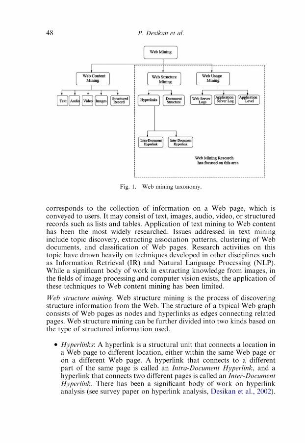
corresponds to the collection of information on a Web page, which isconveyed to users. It may consist of text, images, audio, video, or structuredrecords such as lists and tables. Application of text mining to Web contenthas been the most widely researched. Issues addressed in text mininginclude topic discovery, extracting association patterns, clustering of Webdocuments, and classification of Web pages. Research activities on thistopic have drawn heavily on techniques developed in other disciplines suchas Information Retrieval (IR) and Natural Language Processing (NLP).While a significant body of work in extracting knowledge from images, inthe fields of image processing and computer vision exists, the application ofthese techniques to Web content mining has been limited.
Web structure mining. Web structure mining is the process of discoveringstructure information from the Web. The structure of a typical Web graphconsists of Web pages as nodes and hyperlinks as edges connecting relatedpages. Web structure mining can be further divided into two kinds based onthe type of structured information used.
� Hyperlinks: A hyperlink is a structural unit that connects a location ina Web page to different location, either within the same Web page oron a different Web page. A hyperlink that connects to a differentpart of the same page is called an Intra-Document Hyperlink, and ahyperlink that connects two different pages is called an Inter-DocumentHyperlink. There has been a significant body of work on hyperlinkanalysis (see survey paper on hyperlink analysis, Desikan et al., 2002).
Fig. 1. Web mining taxonomy.
P. Desikan et al.48

� Document structure: The content within a Web page can also beorganized in a tree-structured format, based on the various HTML andXML tags within the page. Here, mining efforts have focused onautomatically extracting document object model (DOM) structures outof documents.
Web usage mining. Web usage mining is the application of data miningtechniques to discover interesting usage patterns fromWeb data, in order tounderstand and better serve the needs of Web-based applications. Usagedata captures the identity or origin of Web users along with their browsingbehavior at a website. Web usage mining itself is further classifieddepending on the kind of usage data used:
� Web server data: The user logs are collected by Web server. Typicaldata includes IP address, page reference, and access time.� Application server data: Commercial application servers, for example,Weblogic, etc. have significant features in the framework to enablee-commerce applications to be built on top of them with little effort.A key feature is the ability to track various kinds of business eventsand log them in application server logs.� Application level data: New kinds of events can always be defined in anapplication, and logging can be turned on for them—generatinghistories of these specially defined events.
2.2 Web mining techniques—state-of-the-art
Enabling technologies such as the Internet has not only generated a newkind of data such as the Web data, but has also generated a new class oftechniques that are associated with this kind of data and applications basedon this platform. For example, ease of obtaining user feedback resulted inobtaining data and developing new techniques for collaborative filtering.The relation between content and structure of the Web has itself led todeveloping a new class of relevance rank measures. Web usage datacollection itself has given rise to new kinds of problems and techniques toaddress them, such as user-session identification, user identification, spamdetection etc. Thus the Web has not only generated new kinds of data buthas opened a series of new problems that can be addressed with availabilityof such data and its applications on the Web, which are different fromtraditional data mining approaches. In the following paragraph we discussthe state-of-art in Web mining research. Web mining techniques have alsoadopted significant ideas from the field of information retrieval. However,our focus in this chapter is restricted to core Web mining techniques and wedo not delve into depth in the large area of information retrieval.The interest of research community and the rapid growth of work in this
area have resulted in significant research contributions which have been
Ch. 2. Web Mining for Business Computing 49

summarized in a number of surveys and book chapters over the past fewyears (Cooley et al., 1997; Kosala and Blockeel, 2000; Srivastava et al., 2004).Research on Web content mining has focused on issues such as extractinginformation from structured and unstructured data and integratinginformation from various sources of content. Earlier work on Web contentmining can be found in Kosala’s work (Kosala and Blockeel, 2000). Webcontent mining together has found its utility in a variety of applications suchas Web page categorization and topic distillation. A special issue on Webcontent mining (Liu and Chang, 2004) captures the recent issues addressedby the research community in the area. Web structure mining has focusedprimarily on hyperlink analysis. A survey on hyperlink analysis techniquesand a methodology to pursue research has been proposed by Desikan et al.(2002). Most of these techniques can be used independently or in conjunctionwith techniques proposed with Web content and Web usage. The mostpopular application is ranking of Web pages. PageRank (Page et al., 1998),developed by Google founders, is a popular metric for ranking theimportance of hypertext documents for Web search. The key idea inPageRank is that a page has a high rank if many highly ranked pages point itto, and hence the rank of a page depends upon the ranks of pages pointing toit. Another popular measure is hub and authority scores. The underlyingmodel for computing these scores is a bipartite graph (Kleinberg, 1998). TheWeb pages are modeled as ‘‘fans’’ and ‘‘centers’’ of a bipartite core, wherea ‘‘fan’’ is regarded as a hub page and ‘‘center’’ as an authority page. For agiven query, a set of relevant pages is retrieved. And for each page in such aset, a hub score and an authority score (Kleinberg, 1998).Web usage data has is the key to understand user’s perspective of the
Web, while content and structure reflect the creator’s perspective. Under-standing user profiles and user navigation patterns for better adaptivewebsites and predicting user access patterns has evoked interest to theresearch and the business community. The primary step for Web usagemining is pre-processing the user log data, such as to separate Web pagereferences into those made for navigational purposes and those made forcontent purposes (Cooley et al., 1999). The concept of adaptive Web wasintroduced by researchers from University of Washington, Seattle(Perkowitz and Etzioni, 1997). Markov models have been the most popularform of techniques to predict user behavior (Pirolli and Pitkow, 1999;Sarukkai, 1999; Zhu et al. 2002). A more detailed information aboutvarious aspects of Web usage mining techniques can be found in a recentextensive survey on this topic (Mobasher, 2005).
3 How Web mining can enhance major business functions
This section discusses existing and potential efforts in the application ofWeb mining techniques to the major functional areas of businesses. Some
P. Desikan et al.50

examples of deployed systems, as well as frameworks for emergingapplications yet-to-be-built, are discussed. It should be noted that theexamples are should not be regarded as solutions to all problems within thebusiness function area they are cited in. Their purpose is to illustrate thatWeb mining techniques have been applied successfully to handle certainkind of problems, providing evidence of their utility. Table 1 provides thesummary of how Web mining techniques have been successfully applied toaddress various issues that arise in business functions.
3.1 Sales
3.1.1 Product recommendationsRecommending products to customers is a key issue for all businesses.
Currently, traditional brick-and-mortar stores have to rely on datacollected explicitly from customers through surveys to offer customer-centric recommendations. However, the advent of e-commerce not onlyenables a level of personalization in customer-to-store interaction that isfar greater than imaginable in the physical world, but also leads tounprecedented levels of data collection, especially about the ‘‘process ofshopping.’’ The desire to understand individual customer shoppingbehavior and psychology in detail through data mining has led tosignificant advances in online customer-relationship management (e-CRM),
Table 1
Summary of how Web mining techniques are applicable to different business functions
Area Function Application Technique
Sales Product marketing Product
recommendations
Association rules
Consumer marketing Product trends Time series data mining
Customer service Expert-driven
recommendations
Association rules, text
mining, link analysis
Purchasing Shipping and inventory Inventory management Clustering, association
rules, forecasting
Operations Human resources HR call centers Sequence similarities,
clustering, association
rules
Sales management Sales leads identification
and assignment
Multi-stage supervised
learning
Fiscal management Fraud detection Link mining
Information technology Developer duplication
reduction
Clustering, text mining
Business process
management
Process mining Clustering, association
rules
Ch. 2. Web Mining for Business Computing 51
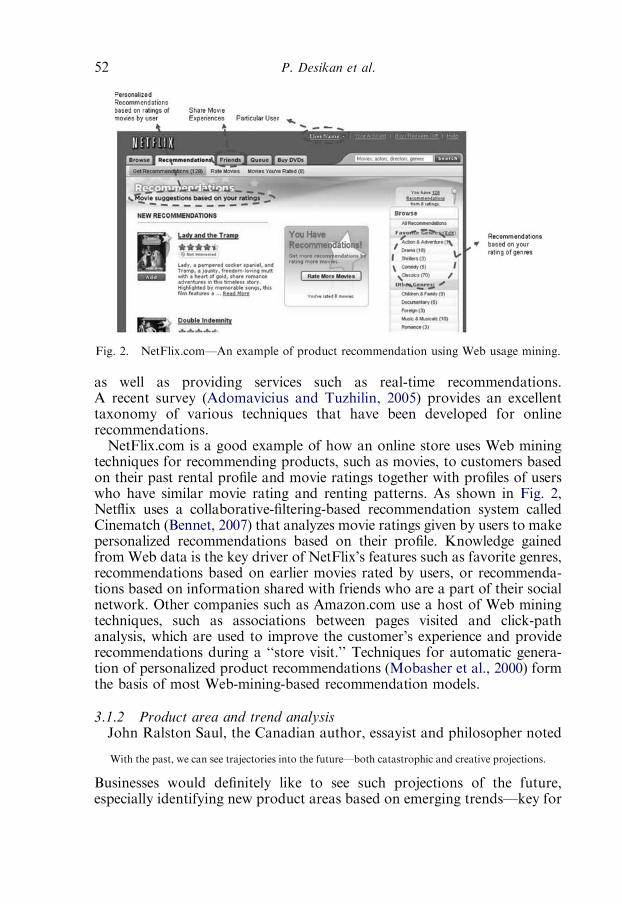
as well as providing services such as real-time recommendations.A recent survey (Adomavicius and Tuzhilin, 2005) provides an excellenttaxonomy of various techniques that have been developed for onlinerecommendations.NetFlix.com is a good example of how an online store uses Web mining
techniques for recommending products, such as movies, to customers basedon their past rental profile and movie ratings together with profiles of userswho have similar movie rating and renting patterns. As shown in Fig. 2,Netflix uses a collaborative-filtering-based recommendation system calledCinematch (Bennet, 2007) that analyzes movie ratings given by users to makepersonalized recommendations based on their profile. Knowledge gainedfromWeb data is the key driver of NetFlix’s features such as favorite genres,recommendations based on earlier movies rated by users, or recommenda-tions based on information shared with friends who are a part of their socialnetwork. Other companies such as Amazon.com use a host of Web miningtechniques, such as associations between pages visited and click-pathanalysis, which are used to improve the customer’s experience and providerecommendations during a ‘‘store visit.’’ Techniques for automatic genera-tion of personalized product recommendations (Mobasher et al., 2000) formthe basis of most Web-mining-based recommendation models.
3.1.2 Product area and trend analysisJohn Ralston Saul, the Canadian author, essayist and philosopher noted
With the past, we can see trajectories into the future—both catastrophic and creative projections.
Businesses would definitely like to see such projections of the future,especially identifying new product areas based on emerging trends—key for
Fig. 2. NetFlix.com—An example of product recommendation using Web usage mining.
P. Desikan et al.52
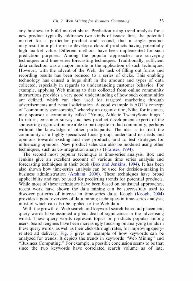
any business to build market share. Prediction using trend analysis for anew product typically addresses two kinds of issues: first, the potentialmarket for a particular product and second, that a single productmay result in a platform to develop a class of products having potentiallyhigh market value. Different methods have been implemented for suchprediction purposes. Among the popular approaches are surveyingtechniques and time-series forecasting techniques. Traditionally, sufficientdata collection was a major hurdle in the application of such techniques.However, with the advent of the Web, the task of filling out forms andrecording results has been reduced to a series of clicks. This enablingtechnology has caused a huge shift in the amount and types of datacollected, especially in regards to understanding customer behavior. Forexample, applying Web mining to data collected from online communityinteractions provides a very good understanding of how such communitiesare defined, which can then used for targeted marketing throughadvertisements and e-mail solicitation. A good example is AOL’s conceptof ‘‘community sponsorship,’’ whereby an organization, Nike, for instance,may sponsor a community called ‘‘Young Athletic TwentySomethings.’’In return, consumer survey and new product development experts of thesponsoring organization are able to participate in that community, perhapswithout the knowledge of other participants. The idea is to treat thecommunity as a highly specialized focus group, understand its needs andopinions towards existing and new products, and to test strategies forinfluencing opinions. New product sales can also be modeled using othertechniques, such as co-integration analysis (Franses, 1994).The second most popular technique is time-series analysis. Box and
Jenkins give an excellent account of various time series analysis andforecasting techniques in their book (Box and Jenkins, 1994). It has beenalso shown how time-series analysis can be used for decision-making inbusiness administration (Arsham, 2006). These techniques have broadapplicability and can be used for predicting trends for potential products.While most of these techniques have been based on statistical approaches,recent work have shown the data mining can be successfully used todiscover patterns of interest in time-series data. Keogh (Keogh, 2004)provides a good overview of data mining techniques in time-series analysis,most of which can also be applied to the Web data.With the growth of Web search and keyword search-based ad placement,
query words have assumed a great deal of significance in the advertisingworld. These query words represent topics or products popular amongusers. Search engines have been increasingly focusing on analyzing trends inthese query words, as well as their click-through rates, for improving query-related ad delivery. Fig. 3 gives an example of how keywords can beanalyzed for trends. It depicts the trends in keywords ‘‘Web Mining’’ and‘‘Business Computing.’’ For example, a possible conclusion seems to be thatsince the two keywords have correlated search volume as of late,
Ch. 2. Web Mining for Business Computing 53
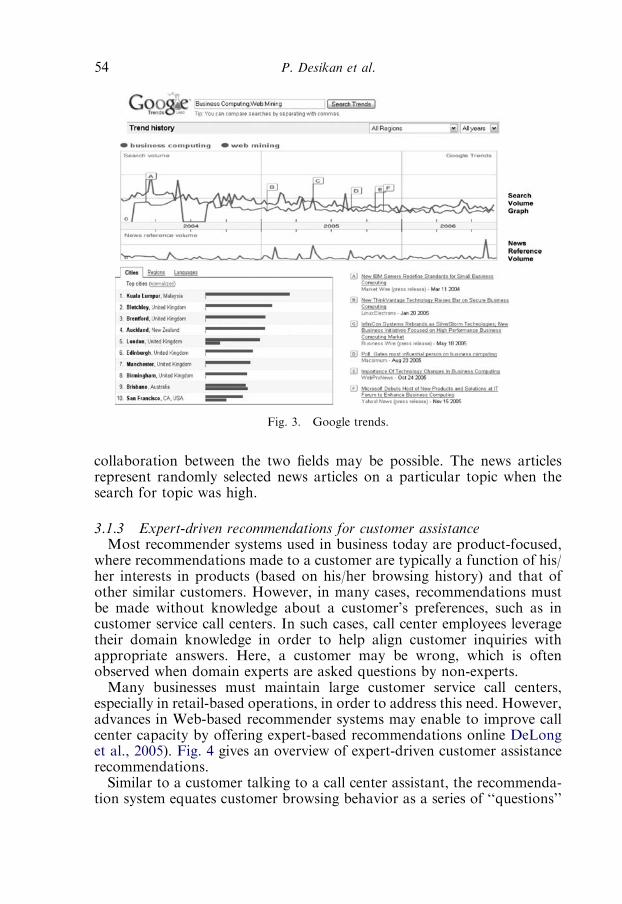
collaboration between the two fields may be possible. The news articlesrepresent randomly selected news articles on a particular topic when thesearch for topic was high.
3.1.3 Expert-driven recommendations for customer assistanceMost recommender systems used in business today are product-focused,
where recommendations made to a customer are typically a function of his/her interests in products (based on his/her browsing history) and that ofother similar customers. However, in many cases, recommendations mustbe made without knowledge about a customer’s preferences, such as incustomer service call centers. In such cases, call center employees leveragetheir domain knowledge in order to help align customer inquiries withappropriate answers. Here, a customer may be wrong, which is oftenobserved when domain experts are asked questions by non-experts.Many businesses must maintain large customer service call centers,
especially in retail-based operations, in order to address this need. However,advances in Web-based recommender systems may enable to improve callcenter capacity by offering expert-based recommendations online DeLonget al., 2005). Fig. 4 gives an overview of expert-driven customer assistancerecommendations.Similar to a customer talking to a call center assistant, the recommenda-
tion system equates customer browsing behavior as a series of ‘‘questions’’
Fig. 3. Google trends.
P. Desikan et al.54

the customer wants answered or, more generally, expressions of interest inthe topic matter of a clicked-on Web page. Given the order and topicmatter covered by such sequences of clicks, the recommendation systemcontinuously refines its recommendations, which are not themselves directlya function of customer interest. Rather, they are generated by querying anabstract representation of customer service website, called a ‘‘concept-pagegraph.’’ This graph contains a ranked set of topic/Web page combinations,and as the customer clicks through the website, the system looks for Webpages best capturing the topics that a customer is seeking to know moreabout. And since their browsing behavior helps determine the questionsthey want answered, the eventual recommendations are more likely find thecorrect answer to their question, rather than a potentially misleading onebased on interest alone.
3.2 Purchasing
3.2.1 Predictive inventory managementA significant cost for a business that sells large quantities of products is
the maintenance of an inventory management system to support sales. Thegoal of inventory management is to keep the inventory acquisition andmaintenance costs low while simultaneously maximizing customer satisfac-tion through product availability. As such, inventory management systemsmust keep track of customer product demand through sales trend andmarket analysis. By analyzing transaction data for purchasing trends,inventory needs can addressed in a pre-emptive fashion, improvingefficiency by enabling ‘‘just-in-time’’ inventory.As the Internet has permeated business computing, the task of browsing
and purchasing products has been reduced to a series of clicks. This hasmade shopping extremely simple for customers and has lowered the barrierfor businesses to obtain detailed customer feedback and shopping behavior
Recommender System
Web Usage Logs<seq1, seq2, ...>
Concept-PageGraph
<page_id, topic_id>
Customer
Browsing Sequence <p1, p2, p4, p7...>
Recommendations
Fig. 4. Overview of expert-driven customer assistance recommendations.
Ch. 2. Web Mining for Business Computing 55
data. And though Web mining techniques have provided an excellentframework for personalized shopping, as well as improved direct marketingand advertisement, it can also aid companies in understanding customeraccess and purchasing patterns for inventory management at a very detailedlevel.Web mining techniques can improve inventory management in a variety
of ways. First, using techniques such as Web content mining to search theWeb—including competitors’ websites—businesses can discover new oralternate vendors and third-party manufacturers. Second, trend analysisusing Web usage mining can yield valuable information about potentiallylatent relationships between products, helping gauge demand for one ormore products based on the sales of others. Taken together, the identifi-cation of inventory gaps (where there is demand for a product not yetstocked) can be addressed and added to inventory at levels correspondingto estimated demand from product relationship analysis.Amazon.com, again, is a great example. As it became one of the largest
B2C websites, its ever-increasing customer base and product breadth(and depth) demanded an efficient inventory management system. As such,Amazon.com adopted advanced Web mining techniques to manage andplan material resource availability. These techniques have enabledAmazon.com to decrease costs incurred from idle stock maintenance andconsequently increase product choice for customers, greatly increasingAmazon’s revenue. By taking advantage of Web usage mining techniquesand applying them to website usage data, transaction data, and externalwebsite data, other companies can reap the benefits of such predictiveinventory management.
3.3 Operations
3.3.1 Human resources call centersHuman resource (HR) departments of large companies are faced with
answering many policy, benefits, and payroll related questions fromemployees. As the size of the company grows, the task becomes moredifficult as they not only need to handle the number of employees, but alsoconsider other issues such as geographically local policies and issues. Anoften-used approach of handling this problem is to have ‘‘call centers,’’where human representatives provide expert assistance to employeesthrough telephone conversations. Due in part to the cost associated withcall centers, many companies have also published all relevant policy andprocess information to their corporate intranet websites for easy perusal byemployees. However, in the face of such large repositories of detailedcontent, many employees tend to still primarily seek the advice of humanrepresentatives at call centers to help them more quickly sort through theirpolicy and procedure questions, resulting in call center escalation.
P. Desikan et al.56
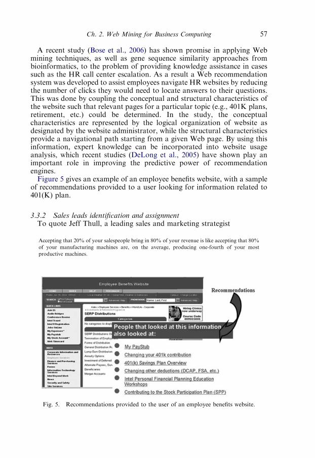
A recent study (Bose et al., 2006) has shown promise in applying Webmining techniques, as well as gene sequence similarity approaches frombioinformatics, to the problem of providing knowledge assistance in casessuch as the HR call center escalation. As a result a Web recommendationsystem was developed to assist employees navigate HR websites by reducingthe number of clicks they would need to locate answers to their questions.This was done by coupling the conceptual and structural characteristics ofthe website such that relevant pages for a particular topic (e.g., 401K plans,retirement, etc.) could be determined. In the study, the conceptualcharacteristics are represented by the logical organization of website asdesignated by the website administrator, while the structural characteristicsprovide a navigational path starting from a given Web page. By using thisinformation, expert knowledge can be incorporated into website usageanalysis, which recent studies (DeLong et al., 2005) have shown play animportant role in improving the predictive power of recommendationengines.Figure 5 gives an example of an employee benefits website, with a sample
of recommendations provided to a user looking for information related to401(K) plan.
3.3.2 Sales leads identification and assignmentTo quote Jeff Thull, a leading sales and marketing strategist
Accepting that 20% of your salespeople bring in 80% of your revenue is like accepting that 80%
of your manufacturing machines are, on the average, producing one-fourth of your most
productive machines.
Fig. 5. Recommendations provided to the user of an employee benefits website.
Ch. 2. Web Mining for Business Computing 57

In many businesses, an effective way of countering this problem is todevelop a process (or system) that will allow sales managers to learn frompast performance and track their current performance, both qualitativelyand quantitatively. With the Internet, a number of Web-based businesseshave emerged to enable customer-relationship management (CRM), arelated approach used to collect, store, and analyze customer information.For example, Salesforce.com (http://www.salesforce.com) offers Web-basedinfrastructure for CRM to companies. Web-based approaches enable easycustomization and integration of different application tools, as well asgeographical independence of viewing the CRM data due to the usage ofa Web-based interface. Macroscopic and microscopic (detailed) viewsand spatio-temporal partitions of information are also possible. Further,real-time dashboards allow easy visualization of various parameters andtheir statistical properties (e.g., means, medians, standard deviation).Commonly, tools for more sophisticated statistical analysis of the data areavailable in such applications.However, much of the burden of analysis and interpretation of such data
lies with the sales managers. Given the number of types of data collectedand possible analysis techniques that can be applied, it becomes difficult fora sales manager to apply all possible techniques and search for interestingresults. As such, many sales managers will use only a few parameters foranalysis on a daily basis. Additionally, the learning curve for this process isslow due to manual effort required in learning which parameters areimportant. Effective analysis is, therefore, made that much more difficultand cumbersome due to limited analytical resources and constraints on thesales manager’s time, which can result in errors and the inability to properlyforecast emerging leads.In sales leads identification, traditional sources of information, such as
phone calls, are supplemented by Web data, providing an additional meansof collecting information about buyers. For example, eBay (http://www.ebay.com/) creates behavior profiles about the buyers (and sellers) ofproducts on their Web portal. Web usage data such as products bought andbrowsed for by buyers provide critical sales lead information. For similarportals, a buyer can be a group of individuals, a small business, or a largeorganization, depending upon its type (e.g., customer-to-customer, customer-to-business, or business-to-business e-commerce). Web content data fromthese external websites can be analyzed using Web content mining to helpidentify new customers and understand their requirements. Competitor’swebsites can be used to learn about their past performance and customers, aswell as helping identify competitors in different geographical regions. Thisrich information about buyers can be harnessed by an enterprise todetermine the most profitable markets, find new sales leads, and alignthem with a business’s offerings. Here, Web mining approaches can play animportant role in identifying connections between various customers,analyzing them, and understanding their various business impacts.
P. Desikan et al.58

3.3.3 Fraud analysisThe Internet has dramatically changed the ways in which businesses
sell products. There are now many well-established Internet sites fore-commerce, and huge numbers of items have been bought and sold online.Meanwhile, fraudulent attempts to unjustly obtain property on websiteshave also been increasing. Although a great deal of effort has beenexpended in investigating and preventing Internet fraud, criminals haveshown they are also capable of quickly adapting to existing defensivemethods and continue to create more sophisticated ways of perpetratingfraud. Some Internet fraud, such as shilling, also exists in offline commerce.However, the frequency of such fraud has dramatically increased in onlinee-commerce applications due to its ease of implementation in an onlinesetting. While some fraudulent activities are ignored when detected, othersare more serious, involve large sums of lost money and property, and canresult in lawsuits brought by their victims.Much Internet-based fraud is perpetrated in a cooperative manner among
multiple associates. For example, in online auction shilling, fake customers(who are actually associates of a fraudulent seller) pretend not to have anyconnection with the seller and raise the bid price so that the seller’s item issold at a higher price than its real value. Such associates are called shills,though shilling can be perpetrated without human associates. A sellercan have multiple ids and pose as different customers simultaneously byparticipating in a single auction using multiple computers having differentIP addresses, pretending to be different bidders. Detecting such fraud oftenmeans tracking the relationships between sellers and customers over aperiod of time. Clearly, non-automated techniques of accomplishing thistask on a wide scale will incur significant costs.For addressing such issues, Web mining techniques have risen to
prominence through their capacity to automatically detect ‘‘fraudulentbehavior’’ in Web usage data. Since Web mining techniques are oftenfocused on discovering relationships in usage, content, and transactiondata, they can be readily applied to analyzing the relationships amongpeople participating in online trading. As previously mentioned, muchInternet fraud is perpetrated in cooperation with multiple ‘‘associates.’’In order to detect such fraudulent activity, graph mining techniques can beused to uncover latent relationships between associates by finding graphswith similar topological structures. Since a number of frauds may beperpetrated by the same group of fraudsters, identifying the group’s otherfrauds can be made possible through these techniques, which have beenexploited not only for detecting fraud in e-commerce, but also for anti-terrorism, financial crime detection, and spam detection.
3.3.4 Developer duplication reductionMany businesses, both large and small, maintain one or more internal
application development units. Thus, at any given time, there may be
Ch. 2. Web Mining for Business Computing 59

hundreds, if not thousands, of projects being developed, deployed, andmaintained concurrently. Due to overlapping business processes (i.e.,human resources and fiscal administration) and multiple project develop-ment groups, duplication of source code often occurs (Rajapakse andJarzabek, 2005) and (Kapser and Godfrey, 2003). Given the non-trivial costof application development, mitigating such duplication is critical. Sourcecode consistency is also an issue, for example, to prevent a case where onlyone of two duplicate segments is updated to address a bug and/or featureaddition.Turnkey solutions for source code duplication are already available, but
they suffer from two major problems:
� They are not able to address code which is functionally similar, butsyntactically different.� They only detect duplication after it has already occurred.
The goal of a full-featured duplication detection system will be to addressexisting and potential duplication—the latter of which is currentlyunavailable. However, Web mining methods may offer a solution.Many businesses maintain intranets containing corporate policy informa-
tion, best practices manuals, contact information, and project details—thelast of which is of particular interest here. Assuming project informationis kept current, it is possible to use Web mining techniques to identifyfunctionality that is potentially duplicative, oftentimes syntacticallydifferent functions may be described using similar language.Figure 6 gives an overview of a possible approach for identifying
potential duplication among multiple projects. First, the project Web pagesand documents must be extracted from the intranet. Next, each document issplit into fragments using common separators (periods, commas, bulletpoints, new lines, etc.). These fragments form the most basic element ofcomparison—the smallest entity capable of expressing a single thought.Using clustering techniques, these fragments can then be grouped intocollections of similar fragments. When two or more fragments are part ofthe same collection, but come from different projects, potential duplication
Clusters of Similar Fragments
Intranet Project Info
Fragmentation<frag_id, doc_id>
Cluster “A” f1, f4, f7
Cluster “B” f2, f3
Cluster “C” f5, f6
Cluster Fragments< f1, f2, f3, f4, ...>
Fig. 6. Duplication candidate process overview.
P. Desikan et al.60
has been identified. These fragments may then be red-flagged and broughtto the attention of affected project managers.
3.3.5 Business process miningBusiness process mining, also called workflow mining, reveals how
existing processes work and can provide considerable return on investment(ROI) when used to discover new process efficiencies. In the context of theWorld Wide Web, business process mining can be defined as the task ofextracting useful process-related information from the click stream of usersof a website or the usage logs collected by the Web server.For example, mining of market-basket data to understand shopping
behavior is perhaps the most well-known and popular application of Webmining. Similarly, one can find better understanding of the shipping processby modeling customer browsing behavior as a state transition diagramwhile he/she shops online. To implement such a system, Web usage logs andclick stream data obtained from servers can be transformed into an XMLformat. These event logs can then be cleaned and the temporal ordering ofbusiness processes inferred. One can then combine Web usage mining withWeb structure mining. By determining the number of traversals (usage) oneach link (structure), one can estimate the transition probabilities betweendifferent states. Using these probabilities, entire business process modelscan be benchmarked and measured for performance increases/decreases.The discovered process model can also be checked for conformance withpreviously discovered models. Here, an anomaly detection system can alsobe to identify deviation in existing business process behavior. Srivastavaand Mobasher (Srivastava and Mobasher, 1997) give an example of such astate transition diagram modeling a shopping transaction in a website,shown in Fig. 7.One can also analyze ‘‘process outcome’’ data to understand the value of
various parts (e.g., states) of the process model (i.e., the impact of variousstates on the probability of desired/undesired outcomes). The results ofsuch analysis can be used to help develop strategies for increasing (ordecreasing) the probabilities of desired outcomes. A possible end objectiveof this business process mining would be to maximize the probability ofreaching the final state while simultaneously maximizing the expectednumber of sold products (or value of sold products) from each visit,conduct a sensitivity analysis of the state transition probabilities, andidentify appropriate promotion opportunities.In addition to the above-mentioned example, business process mining can
also used for e-mail traffic, we can discover how people work and interactwith each other in an organization. We can see what kinds of patterns existin workflow processes and answer questions like do people hand-over theirtasks to others, do they sub-contract, do they work together or do theywork on similar tasks. It thereby helps in determining the process, data,organizational, and social structure.
Ch. 2. Web Mining for Business Computing 61

Sometimes, the information contained in Web server logs is incomplete ornoisy or fine-grained or specific to an application which makes pre-processing a bit more difficult and challenging. Research has to be done inextracting business process models from the server logs. By leveragingbusiness process mining properly, we can re-engineer the business processby reducing work-in-progress, adding additional resources to increase thecapacity or eliminating or improving the efficiency of bottleneck processes,thereby boosting the performance of businesses.
4 Gaps in existing technology
Though Web mining techniques can be extremely useful to businesses,there are gaps which must often be bridged (or completely dealt with) inorder to properly leverage Web mining’s potential. In this section, wediscuss a few such important gaps and how these can be addressed.
4.1 Lack of data preparation for Web mining
To properly apply Web mining in a production setting (e.g., recommend-ing products to customers), data stored in archival systems must be linkedback to online applications. As such, there must be processes in place toclean, transform, and move large segments of data back into a setting,where these can be accessed by Web mining applications quickly andcontinuously. This often means removing extraneous fields and converting
Fig. 7. State transition diagram modeling a shopping transaction in a website (Srivastava
and Mobasher, 1997).
P. Desikan et al.62

textual identifiers (names, products, etc.) into numerical identifiers to makethe processing of large amounts of transactional data quick. For instance,segmenting data into one-month intervals can cut down on expendedcomputing resources and to ensure that relevant trends are identified byWeb mining techniques, provided there is sufficient transactional activity.Additionally, databases for these kinds of intermediate calculations toreduce repeat computations have to be developed. Web mining is oftencomputationally expensive, thus efforts to maximize efficiency areimportant.
4.2 Under-utilization of domain knowledge repositories
Businesses have long made use of domain knowledge repositories tostore information about business processes, policies, and projects, and ifthey are utilized in a Web mining setting, it becomes ever more paramountto manage it. For instance, corporate intranets provide a wealth ofinformation that is useful in expert-oriented recommendations (e.g.,customer service) and duplication reduction, but the repository itself mustbe up-to-date and properly maintained from time to time. One of the bestways to ensure an intranet’s ‘‘freshness’’ is to maintain it with a contentmanagement system (CMS) allowing non-professionals to update thewebsite and distributing the responsibility to internal stakeholders.
4.3 Under-utilization of Web log data
Most companies keep track of Web browsing behavior of employees bycollecting Web logs mostly for security purposes. However, as seen fromprevious successful applications of Web mining techniques on such kindsof data, companies could utilize this information to better serve theiremployees. For example, one of the key issues that is usually dealt byhuman resources department is to keep employees motivated and retainthem. A common approach is to offer perks and bonuses in various formsto satisfy the employee. However, most policies are ‘‘corporate-centric’’ andare not geared towards ‘‘employee-centric.’’ With the advance of Webmining techniques, it is now possible to understand employees’ interests in abetter way. Two kinds of techniques can be employed. First, is to mine thebehavior of employees in company policy and benefits website, in order tounderstand what employees are looking for. For example, employeesbrowsing retirement benefits related website, could be offered a betterretirement package. Other examples include, tuition waiver for employeeslooking on pursuing professional development course, or a travel packagedeal to an employee who has shown interest in traveling. A differentdimension is to use trend analysis to see what’s new and popular in market,such as a new MP3 player, and offer perks in form of such as products.
Ch. 2. Web Mining for Business Computing 63

Of course, a key issue in such kind of techniques is privacy. Privacypreserving data mining is a currently a hot area of research. Also, it hasbeen studied and shown from examples such as Amazon that people arewilling to compromise a certain level of privacy to gain the benefits offered.
5 Looking ahead: The future of Web mining in business
We believe that the future of Web mining is entwined with the emergingneeds of businesses, and the development of techniques fueled by therecognition of gaps or areas of improvement in existing techniques. Thissection examines what is on the horizon for Web mining, the nascent areascurrently under research, and how they can help in a business computingsetting.
5.1 Microformats
It is very important to not only to present the right content on a website,but also in the right format. For example, a first step in formatting for theWeb was the use of oHTMLW to give the browser’s ability to parse andpresent text in a more readable and presentable format. However,researchers soon developed formats with higher semantics and present-ability, for example, XML and CSS, for efficient processing of content andextracting useful information. XML is used to store data in formats suchthat automatic processing can be done to extract meaningful information(not just for presenting it in a website). Today, the trend is moving moretowards ‘‘micro-formats’’ which capture the best of XML and CSS.Microformats are design principles for formats and not another newlanguage. They provide a way of thinking about data, which will providehumans a better understanding of the data. They are currently widely usedin websites such as blogs. With such new structured data, there arises needfor NLP and Web content mining techniques such as data extraction,information integration, knowledge synthesis, template detection, andpage-segmentation. This leads to the suggestion for the corporatebusinesses to decide on right kind of format to best utilize the data forprocessing, analysis, and presentation.
5.2 Mining and incorporating sentiments
Even though automated conceptual discovery from text is still relativelynew, difficult, and imperfect, accurately connecting that knowledge tosentiment information—how someone feels about something—is evenharder. Natural language processing techniques, melded with Web mining,hold great promise in this area. To understand how someone feels about a
P. Desikan et al.64
particular product, brand, or initiative, and to project that level of under-standing across all customers would give the business a more accuraterepresentation of what customers think to date. Applied to the Web, onecould think of an application that collects such topic/sentiment informationfrom the Internet, and returns that information to a business. Accomplish-ing this would open up many marketing possibilities.
5.3 e-CRM to p-CRM
Traditionally, brick-and-mortar stores have been organized in a product-oriented manner, with aisles for various product categories. However,success of online e-CRM initiatives in the online world in building customerloyalty is not hidden from CRM practitioners in the physical world, whichwe refer to as p-CRM for clarity in this chapter. Additionally, thesignificance of physical stores has motivated a number of online businessesto open physical stores to serve ‘‘real people’’ (Earle, 2005). Manybusinesses have also moved from running their online and physical storesseparately to integrating both, in order to better serve their customers(Stuart, 2000). Carp (Carp, 2001) points out that although the onlinepresence of a business does affect its physical division of its business, peoplestill find entertainment value in shopping in malls and other physical stores.Finally, people prefer to get a feel of products before purchase, and henceprefer to go out to shop instead of shopping online. From theseobservations, it is evident that physical stores will continue to be thepreferred means of conducting consumer commerce for quite some time.However, margins will be under pressure as they must adopt to competewith online stores. These observations led us to posit the following in ourprevious study (Mane et al., 2005):
Given that detailed knowledge of an individual customer’s habits can provide insight into his/her
preferences and psychology, which can be used to develop a much higher level of trust in a
customer-vendor relationship, the time is ripe for revisiting p-CRM to see what lessons learned
from e-CRM are applicable.
Till recently, a significant roadblock in achieving this vision has been theability to collect and analyze detailed customer data in the physical world,as Underhill’s seminal study (Underhill, 1999) showed, both from cost andcustomer sensitivity perspectives. With advancements in pervasive comput-ing technologies such as mobile Internet access, third-generation wirelesscommunication, RFIDs, handheld devices, and Bluetooth; there has beena significant increase in the ability to collect detailed customer data. Thisraises the possibility of bringing e-CRM style real-time, personalized,customer relationship functions to the physical world. For a more detailedstudy on this, refer to our previous work (Mane et al., 2005).
Ch. 2. Web Mining for Business Computing 65

5.4 Other directions
We have mentioned some of the key issues that should be noted bybusinesses as they proceed to adopt Web mining techniques to improve thebusiness intelligence. However, as claimed earlier, this by no means is anexhaustive list. There are various other issues that need to be addressedfrom a technical perspective in order to determine the framework necessaryto make these techniques more widely applicable to businesses. Forexample, there are host of open areas of research regarding Web mining,such as extraction of structured data from unstructured data or ranking ofWeb pages by integrating semantic relationships between documents, andautomatic derivation of user sentiment. Businesses must also focus on thetypes of data that need to be collected for many Web usage miningtechniques to be possible. Designing the content of websites also plays acrucial role in deciding what kinds of data can be collected. For example,one viewpoint is that pages with Flash-based content, though attractive,are more of broadcast nature and do not easily facilitate the collection ofinformation about customer behavior. However, recent advances intechnologies such as AJAX, which enhance customer/website interaction,not only allow corporations to collect data, but also give the customer a‘‘sense of control’’ leading to an enriched user experience.
6 Conclusion
This chapter examines how technology, such as Web mining, can aidbusinesses in gaining an extra information and intelligence. We provide anintroduction to Web mining and the various techniques associated with it.We briefly update the reader with state-of-art research in this area. Later,we show how these class of techniques can be used effectively to aid variousbusiness functions and provide example applications to illustrate theirapplicability. These examples provide evidence of Web mining’s potential,as well as existing success, in improving business intelligence. Finally, wepoint out gaps in existing technologies and elaborate on future directionsthat should be of interest to the business community at large. In doing so,we also note that we have intentionally left out specific technical details ofexisting and future work, given the introductory nature of this chapter.
Acknowledgments
This work was supported in part by AHPCRC contract numberDAAD19-01-2-0014, by NSF Grant ISS-0308264 and by ARDA grantF30602-03C-0243. This work does not necessarily reflect the position orpolicy of government and no official endorsement should be inferred.
P. Desikan et al.66
We would like to thank the Data Mining Research Group at the Universityof Minnesota for providing valuable feedback.
References
Adomavicius, G., A. Tuzhilin (2005). Towards the next generation of recommender systems: a survey
of the state-of-the-art and possible extensions. IEEE Transactions on Knowledge and Data
Engineering 17, 734–749.
Arsham, H. (2006). Time-critical decision making for business administration. Available at http://
home.ubalt.edu/ntsbarsh/stat-data/Forecast.htm. Retrieved on 2006.
Bennet, J. (2007). The Cinematch system: Operation, scale coverage, accuracy impact. Available at
http://blog.recommenders06.com/wp-content/uploads/2006/09/bennett.pdf. Retrieved and accessed
on July 30.
Bose, A., K. Beemanapalli, J. Srivastava, S. Sahar (2006). Incorporating Concept Hierarchies into Usage
Based Recommendations. WEBKDD, Philadelphia, PA, USA.
Box, G.E., G.M. Jenkins (1994). Time Series Analysis: Forecasting and Control. 3rd ed. Prentice Hall
PTR.
Carp, J. (2001). Clicks vs. bricks: Internet sales affect retail properties. Houston Business Journal
Cooley, R., B. Mobasher, J. Srivastava (1997). Web mining: Information and pattern discovery on the
World Wide Web. 9th IEEE ICTAI.
Cooley, R., B. Mobasher, J. Srivastava (1999). Data preparation for mining World Wide Web browsing
patterns. Knowledge and Information Systems 1(1), 5–32.
DeLong, C., P. Desikan, J. Srivastava (2005). USER (User Sensitive Expert Recommendation): What
non-experts NEED to know, in: Proceedings of WebKDD, Chicago, IL.
Desikan, P., J., Srivastava, V., Kumar, P.N. Tan (2002). Hyperlink analysis: Techniques and applica-
tions. Technical Report 2002-0152, Army High Performance Computing and Research Center.
Earle, S. (2005). From clicks to bricks . . . online retailers coming back down to earth. Feature story.
Available at http://www.specialtyretail.net/issues/december00/feature_bricks.htm. Retrieved on 2005.
Etzioni, O. (1996). The World Wide Web: Quagmire or gold mine? Communications of the ACM 39(11),
65–68.
Franses, Ph.H.B.F. (1994). Modeling new product sales; an application of co-integration analysis.
International Journal of Research in Marketing.
Kapser, C., M.W. Godfrey (2003). Toward a taxonomy of clones in source code: A case study, in:
International Workshop on Evolution of Large-scale Industrial Software Applications, Amsterdam,
The Netherlands.
Keogh, E. (2004). Data mining in time series databases tutorial, in: Proceedings of the IEEE Int.
Conference on Data Mining.
Kleinberg, J.M. (1998). Authoritative sources in hyperlinked environment, in: 9th Annual ACM-SIAM
Symposium on Discrete Algorithms, pp. 668–667.
Kosala, R., H. Blockeel (2000). Web mining research: A survey. SIGKDD Explorations 2(1), 1–15.
Liu, B., K.C.C. Chang (2004). Editorial: Special issue on web content mining. SIGKDD Explorations
special issue on Web Content Mining.
Mane, S., P. Desikan, J. Srivastava (2005). From clicks to bricks: CRM lessons from E-commerce. Technical
report 05-033, Department of Computer Science, University of Minnesota, Minneapolis, USA.
Mobasher, B. (2005). Web usage mining and personalization, in: M.P. Singh (ed.), Practical Handbook
of Internet Computing. CRC Press.
Mobasher, B., R. Cooley, J. Srivastava (2000). Automatic personalization based on web usage mining.
Communications of ACM.
Page, L., S. Brin, R. Motwani, T. Winograd (1998). The pagerank citation ranking: Bringing order to
the web. Stanford Digital Library Technologies
Perkowitz, M., O. Etzioni (1997). Adaptive Web Sites: An AI Challenge. IJCAI.
Ch. 2. Web Mining for Business Computing 67

Pirolli, P., J.E. Pitkow (1999). Distribution of surfer’s path through the World Wide Web: Empirical
characterization. World Wide Web 1, 1–17.
Rajapakse, D.C., S. Jarzabek (2005). An investigation of cloning in web applications, in: Fifth
International Conference on Web Engineering, Sydney, Australia.
Sarukkai, R.R. (1999). Link prediction and path analysis using Markov chains, in: Proceedings of the 9th
World Wide Web Conference.
Srivastava, J., P. Desikan, V. Kumar (2004). Web mining-concepts, applications and research directions.
Data Mining: Next Generation Challenges and Future Directions, MIT/AAAI.
Srivastava, J., B. Mobasher (1997). Panel discussion on ‘‘Web Mining: Hype or Reality?’’, ICTAI.
Stuart, A. (2000). Clicks and bricks. CIO Magazine.
Underhill, P. (1999). Why We Buy: The Science of Shopping. Simon and Schuster, New York.
Zhu, J., J. Hong, J.G. Hughes (2002). Using markov chains for link prediction in adaptive web sites, in:
Proceedings of ACM SIGWEB Hypertext.
P. Desikan et al.68

Adomavicius & Gupta, Eds., Handbooks in Information Systems, Vol. 3
Copyright r 2009 by Emerald Group Publishing Limited
Chapter 3
Current Issues in Keyword Auctions
De Liu455Y Gatton College of Business and Economics, University of Kentucky, Lexington,
KY 40506, USA
Jianqing ChenHaskaynes School of Business, The University of Calgary, Calgary, AB T1N 2N4, Canada
Andrew B. WhinstonMccombs School of Business, The University of Texas at Austin, Austin, TX 78712, USA
Abstract
Search engines developed a unique advertising model a decade ago thatmatched online users with short-text advertisements based on users’ searchkeywords. These keyword-based advertisements, also known as ‘‘sponsoredlinks,’’ are the flagship of the thriving Internet advertising business nowadays.Relatively unknown to online users, however, is the fact that slots for searchengine advertisements are sold by a special kind of auctions which we call‘‘keyword auctions.’’ As the most successful online auctions since eBay’sbusiness-to-consumer auctions, keyword auctions form the backbone of themultibillion dollar search advertising industry. Owing to their newness andsignificance, keyword auctions have captured attention of researchers frominformation systems, computer science, and economics. Many questions havebeen raised, including how to best characterize keyword auctions, why keywordauctions, not other selling mechanisms, are used, and how to design keywordauctions optimally. The purpose of this chapter is to summarize the currentefforts in addressing these questions. In doing so, we highlight the last question,that is, how to design effective auctions for allocating keyword advertisingresources. As keyword auctions are still new, there are still many outstandingissues about keyword auctions. We point out several such issues for futureresearch, including the click-fraud problem associated with keyword auctions.
69
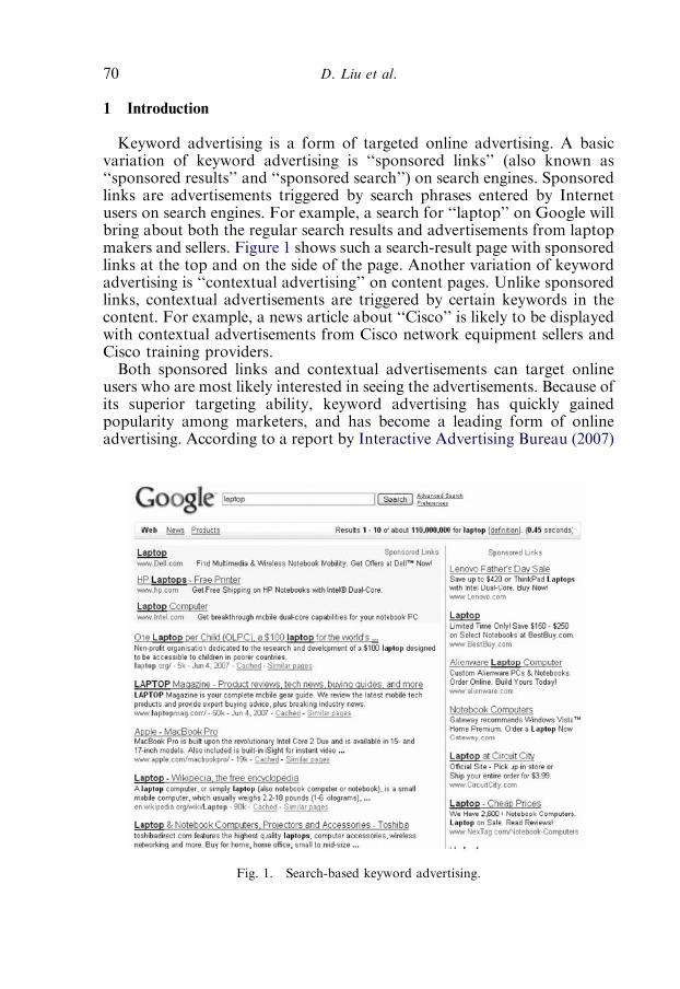
1 Introduction
Keyword advertising is a form of targeted online advertising. A basicvariation of keyword advertising is ‘‘sponsored links’’ (also known as‘‘sponsored results’’ and ‘‘sponsored search’’) on search engines. Sponsoredlinks are advertisements triggered by search phrases entered by Internetusers on search engines. For example, a search for ‘‘laptop’’ on Google willbring about both the regular search results and advertisements from laptopmakers and sellers. Figure 1 shows such a search-result page with sponsoredlinks at the top and on the side of the page. Another variation of keywordadvertising is ‘‘contextual advertising’’ on content pages. Unlike sponsoredlinks, contextual advertisements are triggered by certain keywords in thecontent. For example, a news article about ‘‘Cisco’’ is likely to be displayedwith contextual advertisements from Cisco network equipment sellers andCisco training providers.Both sponsored links and contextual advertisements can target online
users who are most likely interested in seeing the advertisements. Because ofits superior targeting ability, keyword advertising has quickly gainedpopularity among marketers, and has become a leading form of onlineadvertising. According to a report by Interactive Advertising Bureau (2007)
Fig. 1. Search-based keyword advertising.
D. Liu et al.70

and PricewaterhouseCoopers, keyword advertising in the United Statesreached $6.8 billion in total revenue in 2006. eMarketer (2007) predicts themarket for online advertising will rise from $16.9 billion in 2006 to $42billion in 2011, with keyword advertising accounting for about 40% of thetotal revenue.A typical keyword advertising market consists of advertisers and
publishers (i.e., websites), with keyword advertising providers (KAPs) inbetween. There are three key KAPs in the U.S. keyword advertisingmarket: Google, Yahoo!, and MSN adCenter. Figure 2 illustrates Google’skeyword-advertising business model. Google has two main advertisingprograms, Adwords and AdSense. Adwords is Google’s flagship advertisingprogram that interfaces with advertisers. Through Adwords, advertiserscan submit advertisements, choose keywords relevant to their businesses,and pay for the cost of their advertising campaigns. Adwords has separateprograms for sponsored search (Adwords for search) and for contextualadvertising (Adwords for content). In each case, advertisers can choose toplace their advertisements on Google’s site only or on publishers’ sites thatare part of Google’s advertising network. Advertisers can also choose todisplay text, image, or, more recently, video advertisements.AdSense is another Google advertising program that interfaces with
publishers. Publishers from personal blogs to large portals such asCNN.com can participate in Google’s AdSense program to monetize thetraffic to their websites. By signing up with AdSense, publishers agree topublish advertisements and receive payments from Google. Publishersmay choose to display text, image, and video advertisements on their sites.They receive payments from Google on either a per-click or per-thousand-impressions basis.1 AdSense has become the single most important revenuesource for many Web 2.0 companies.This chapter focuses on keyword auctions, which are used by KAPs in
selling their keyword advertising slots to advertisers. A basic form of
Fig. 2. Google’s Adwords and AdSense programs.
1Google is also beta-testing a per-action based service in which a publisher is paid each time a usercarries out a certain action (e.g., a purchase).
Ch. 3. Current Issues in Keyword Auctions 71
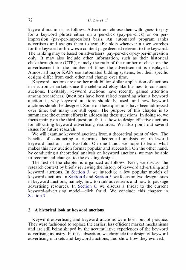
keyword auction is as follows. Advertisers choose their willingness-to-payfor a keyword phrase either on a per-click (pay-per-click) or on per-impression (pay-per-impression) basis. An automated program ranksadvertisers and assigns them to available slots whenever a user searchesfor the keyword or browses a content page deemed relevant to the keyword.The ranking may be based on advertisers’ pay-per-click/pay-per-impressiononly. It may also include other information, such as their historicalclick-through-rate (CTR), namely the ratio of the number of clicks on theadvertisement to the number of times the advertisement is displayed.Almost all major KAPs use automated bidding systems, but their specificdesigns differ from each other and change over time.Keyword auctions are another multibillion-dollar application of auctions
in electronic markets since the celebrated eBay-like business-to-consumerauctions. Inevitably, keyword auctions have recently gained attentionamong researchers. Questions have been raised regarding what a keywordauction is, why keyword auctions should be used, and how keywordauctions should be designed. Some of these questions have been addressedover time, but many are still open. The purpose of this chapter is tosummarize the current efforts in addressing these questions. In doing so, wefocus mainly on the third question, that is, how to design effective auctionsfor allocating keyword advertising resources. We also point out severalissues for future research.We will examine keyword auctions from a theoretical point of view. The
benefits of conducting a rigorous theoretical analysis on real-worldkeyword auctions are two-fold. On one hand, we hope to learn whatmakes this new auction format popular and successful. On the other hand,by conducting a theoretical analysis on keyword auctions, we may be ableto recommend changes to the existing designs.The rest of the chapter is organized as follows. Next, we discuss the
research context by briefly reviewing the history of keyword advertising andkeyword auctions. In Section 3, we introduce a few popular models ofkeyword auctions. In Section 4 and Section 5, we focus on two design issuesin keyword auctions, namely, how to rank advertisers and how to packageadvertising resources. In Section 6, we discuss a threat to the currentkeyword-advertising model—click fraud. We conclude this chapter inSection 7.
2 A historical look at keyword auctions
Keyword advertising and keyword auctions were born out of practice.They were fashioned to replace the earlier, less efficient market mechanismsand are still being shaped by the accumulative experiences of the keywordadvertising industry. In this subsection, we chronicle the design of keywordadvertising markets and keyword auctions, and show how they evolved.
D. Liu et al.72

2.1 Early Internet advertising contracts
In early online advertising, advertising space was sold through advancecontracts. These contracts were negotiated on a case-by-case basis. As suchnegotiations were time-consuming, advertising sales were limited to largeadvertisers (e.g., those paying at least a few thousand dollars per month).These advertising contracts were typically priced in terms of the number ofthousand-page-impressions (cost-per-mille, or CPM). CPM pricing wasborrowed directly from off-line advertising, such as TV, radio, and print,where advertising costs are measured on a CPM basis. The problem withCPM pricing is that it provides no indication as to whether users have paidattention to the advertisement. Advertisers may be concerned that theiradvertisements are pushed to web users without necessarily generating anyimpact. The lack of accountability is reflected in the saying amongmarketing professionals: ‘‘I know that I waste half of my advertisingbudget. The problem is I don’t know which half.’’
2.2 Keyword auctions by GoTo.com
In 1998, a startup company called GoTo.com demonstrated a new proof-of-concept search engine at a technology conference in Monterey,California. At that time, all other search engines sorted search resultsbased purely on algorithm-assessed relevancy. GoTo.com, on the otherhand, devised a plan to let advertisers bid on top positions of the searchresult. Specifically, advertisers can submit their advertisements on chosenwords or phrases (‘‘search terms’’) together with their pay-per-click on theseadvertisements. Once the submitted advertisements are validated byGoTo.com’s editorial team, they will appear as a search result. The highestadvertiser will appear at the top of the result list, the second-highestadvertiser will appear at the second place of the result list, and so on. Eachtime a user clicks on an advertisement, the advertiser will be billed theamount of the bid.GoTo.com’s advertising model contains several key innovations. First,
advertising based on user-entered search terms represents a new form oftargeted advertising that is based on users’ behavior. For example, a userwho searches ‘‘laptop’’ is highly likely in the process of buying a laptop.Keyword-based search engine advertising opens a new era of behavioraltargeted advertising. Second, by billing advertisers only when users click onthe advertisements, GoTo.com provides a partial solution to a longstandingissue of lack of accountability. Clicking on an advertisement indicatesonline users’ interests. Therefore, pay-per-click represents a significant steptoward more accountable advertising.The ability to track behavioral outcomes such as clicks is a crucial
difference between online advertising and its off-line counterparts. The act
Ch. 3. Current Issues in Keyword Auctions 73

of clicking on an advertisement provides an important clue on advertisingeffectiveness. Accumulated information on clicking behavior can be furtherused to fine-tune advertisement placement and content. In such a sense,pay-per-click is a significant leap from the CPM scheme and signifies thehuge potential of online advertising.Finally, the practice of using auctions to sell advertising slots on a
continuous, real-time basis is another innovation. These real-time auctionsallow advertisements to go online a few minutes after a successful bidding.As there is no pre-set minimum spending, auction-based advertising hasthe advantage of tapping into the ‘‘long tail’’ of the advertising market,that is, advertisers who have small spending budgets and are more likely to‘‘do-it-yourself.’’GoTo.com was re-branded as Overture Services in 2001 and acquired by
Yahoo! in 2003. During the process, however, the auction mechanism andthe pay-per-click pricing scheme remained largely unchanged.
2.3 Subsequent innovations by Google
Google, among others, made several key innovations to the keywordadvertising business model. Some of these have become standard features oftoday’s keyword advertising. In the following, we briefly review theseinnovations.
2.3.1 Content vs. advertisingThe initial design by GoTo.com features a ‘‘paid placement’’ model: paid
advertising links are mixed with organic search results so that users cannottell whether a link is paid for. Google, when introducing its own keywordadvertising in 1998, promoted a ‘‘sponsored link’’ model that distinguishedadvertisements from organic search results. In Google’s design, advertise-ments are displayed on the side or on top of the result page with a label‘‘sponsored links.’’ Google’s practice has been welcomed by the industryand policy-makers and has now become standard practice.
2.3.2 Allocation rulesGoogle introduced a new allocation rule in 2002 in its ‘‘Adwords Select’’
program in which listings are ranked not only by bid amount, but also byCTR (later termed as ‘‘quality score’’). Under such a ranking rule, paying ahigh price alone cannot guarantee a high position. An advertiser with a lowCTR will get a lower position than advertisers who bid the same (or slightlylower) but have higher CTRs. In 2006, Google revised its quality scorecalculation to include not only advertisers’ past CTRs but also the qualityof their landing pages. Advertisers with low quality scores are required topay a high minimum bid or they will become inactive.
D. Liu et al.74

Google’s approach to allocation gradually gained acceptance. At thebeginning of 2007, Yahoo! conducted a major overhaul of its onlineadvertising platform that considers both the CTRs of an advertisement andother undisclosed factors. Microsoft adCenter, which came into use only atthe beginning of 2006, used a ranking rule similar to Google’s Adwords.Before that, all of the advertisements displayed on the MSN search enginewere supplied by Yahoo!
2.3.3 Payment rulesIn the keyword auctions used by GoTo.com, bidders pay the amount of
their bids. This way, any decrease in one’s bid will result in less payment. Asa result, bidders have incentives to monitor the next highest bids and makesure their own bids are only slightly higher. The benefits from constantlyadjusting one’s bid create undesirable volatility in the bidding process.Perhaps as a remedy, Google used a different payment rule in theirAdwords Select program. In Adwords Select, bidders do not pay the fullamount of their bids. Instead, they pay the lowest possible to remain abovethe next highest competitor. If the next highest competitor’s bid drops,Google automatically adjusts the advertiser’s payment downward. Thisfeature, termed as ‘‘Adwords Discounter,’’ is essentially an implementationof second-price auctions in a dynamic context. One key advantage of suchan arrangement is that bidders’ payments are no longer directly linked totheir bids. This reduces bidders’ incentive to game the system. Recognizingthis advantage, Yahoo! (Overture) also switched to a similar payment rule.We discuss further the implications of different payment rules in Section 3.
2.3.4 Pricing schemesAs of now, Google’s Adwords for search offers only pay-per-click
advertising. On the other hand, Adwords for content allows advertisers tobid either pay-per-click or pay-per-thousand-impression. Starting spring2007, Google began beta-testing a new billing metric called pay-per-actionwith their Adwords for content. Under pay-per-action metric, advertiserspay only for completed actions of choice, such as a lead, a sale, or a pageview, after a user has followed through the advertisement to the publisher’swebsite.
2.4 Beyond search engine advertising
The idea of using keywords to place most relevant advertisements is notlimited to search engine advertising. In 2003, Google introduced an‘‘AdSense’’ program that allows web publishers to generate advertisingrevenue by receiving advertisements served by Google. AdSense analyzespublishers’ web pages to generate a list of most relevant keywords, whichare subsequently used to select the most appropriate advertisements for
Ch. 3. Current Issues in Keyword Auctions 75
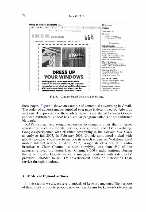
these pages. Figure 3 shows an example of contextual advertising in Gmail.The order of advertisements supplied to a page is determined by Adwordsauctions. The proceeds of these advertisements are shared between Googleand web publishers. Yahoo! has a similar program called Yahoo! PublisherNetwork.KAPs also actively sought expansion to domains other than Internet
advertising, such as mobile devices, video, print, and TV advertising.Google experimented with classified advertising in the Chicago Sun-Timesas early as fall 2005. In February 2006, Google announced a deal withglobal operator Vodafone to include its search engine on Vodafone Live!mobile Internet service. In April 2007, Google struck a deal with radiobroadcaster Clear Channel to start supplying less than 5% of theadvertising inventory across Clear Channel’s 600þ radio stations. Duringthe same month, Google signed a multiyear contract with satellite-TVprovider EchoStar to sell TV advertisement spots on EchoStar’s Dishservice through auctions.
3 Models of keyword auctions
In this section we discuss several models of keyword auctions. The purposeof these models is not to propose new auction designs for keyword-advertising
Fig. 3. Context-based keyword advertising.
D. Liu et al.76

settings but to capture the essence of keyword auctions accurately. Thevalue of these models lies in that they allow the real-world keywordauctions to be analyzed in a simplified theoretical framework.We start by describing the problem setting. There are n advertisers
bidding for m (pn) slots on a specific keyword phrase. Let cij denote thenumber of clicks generated by advertiser i on slot j. In general, cij dependsboth on the relevance of the advertisement and on the prominence of theslot. In light of this, we decompose cij to an advertiser (advertisement)factor (qi) and a slot factor (dj ).
cij ¼ djqi (1)
We interpret the advertiser factor qi as the advertiser i’s CTR. Forexample, everything else being equal, a brand-name advertiser may attractmore clicks and thus have a higher CTR than a non-brand-name advertiser.We interpret the slot factor dj as the click potential of the slot. For example,a slot at the top of a page has higher click potential than a slot at thebottom of the same page.Each advertiser has a valuation-per-click vi. As in most research, we
assume that advertisers know their own valuation-per-click. Though inreality, advertisers may have to learn over time their valuation-per-clickfrom the outcome of the keyword advertising.Each advertiser submits a bid b that is the advertiser’s maximum
willingness-to-pay per click for the keyword phrase. Each time a userinitiates a search for the keyword phrase or requests a content page relatedto the keyword phrase, the auctioneer (KAP) will examine the bids from allparticipating advertisers and determine which advertisements should bedisplayed and in which order according to an allocation rule. If a user clickson a particular advertisement, the advertiser will be charged a pricedetermined by the payment rule of the keyword auction (which we willexplain shortly).The allocation rule and the payment rule used in keyword auctions are
different across different KAPs. For example, until recently, Yahoo! rankedadvertisers strictly by the prices they bid, and advertisers paid the amountthey bid. On the other hand, Google ranks advertisers based on their pricesand their CTRs, and advertisers pay the lowest price that keeps theadvertiser above the next highest-ranked advertiser. We distinguish thefollowing models of keyword auctions by different allocation or paymentrules used.
3.1 Generalized first-price auction
In the early days of keyword auctions, bidders paid the price they bid.Such a format is termed ‘‘generalized first-price (GFP)’’ auctions becausethey essentially extended the first-price auctions to a multiple-object
Ch. 3. Current Issues in Keyword Auctions 77
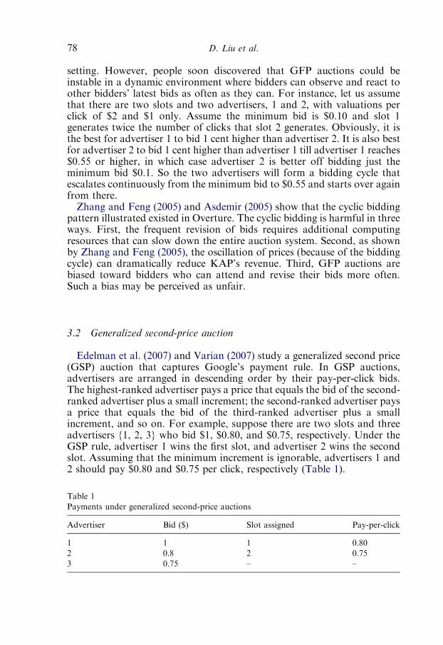
setting. However, people soon discovered that GFP auctions could beinstable in a dynamic environment where bidders can observe and react toother bidders’ latest bids as often as they can. For instance, let us assumethat there are two slots and two advertisers, 1 and 2, with valuations perclick of $2 and $1 only. Assume the minimum bid is $0.10 and slot 1generates twice the number of clicks that slot 2 generates. Obviously, it isthe best for advertiser 1 to bid 1 cent higher than advertiser 2. It is also bestfor advertiser 2 to bid 1 cent higher than advertiser 1 till advertiser 1 reaches$0.55 or higher, in which case advertiser 2 is better off bidding just theminimum bid $0.1. So the two advertisers will form a bidding cycle thatescalates continuously from the minimum bid to $0.55 and starts over againfrom there.Zhang and Feng (2005) and Asdemir (2005) show that the cyclic bidding
pattern illustrated existed in Overture. The cyclic bidding is harmful in threeways. First, the frequent revision of bids requires additional computingresources that can slow down the entire auction system. Second, as shownby Zhang and Feng (2005), the oscillation of prices (because of the biddingcycle) can dramatically reduce KAP’s revenue. Third, GFP auctions arebiased toward bidders who can attend and revise their bids more often.Such a bias may be perceived as unfair.
3.2 Generalized second-price auction
Edelman et al. (2007) and Varian (2007) study a generalized second price(GSP) auction that captures Google’s payment rule. In GSP auctions,advertisers are arranged in descending order by their pay-per-click bids.The highest-ranked advertiser pays a price that equals the bid of the second-ranked advertiser plus a small increment; the second-ranked advertiser paysa price that equals the bid of the third-ranked advertiser plus a smallincrement, and so on. For example, suppose there are two slots and threeadvertisers {1, 2, 3} who bid $1, $0.80, and $0.75, respectively. Under theGSP rule, advertiser 1 wins the first slot, and advertiser 2 wins the secondslot. Assuming that the minimum increment is ignorable, advertisers 1 and2 should pay $0.80 and $0.75 per click, respectively (Table 1).
Table 1
Payments under generalized second-price auctions
Advertiser Bid ($) Slot assigned Pay-per-click
1 1 1 0.80
2 0.8 2 0.75
3 0.75 – –
D. Liu et al.78
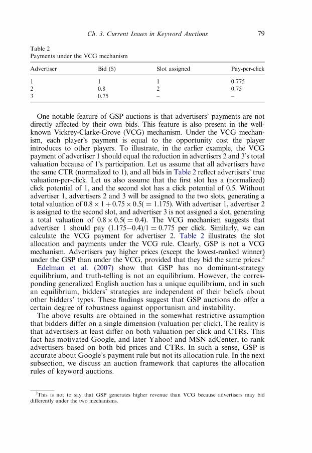
One notable feature of GSP auctions is that advertisers’ payments are notdirectly affected by their own bids. This feature is also present in the well-known Vickrey-Clarke-Grove (VCG) mechanism. Under the VCG mechan-ism, each player’s payment is equal to the opportunity cost the playerintroduces to other players. To illustrate, in the earlier example, the VCGpayment of advertiser 1 should equal the reduction in advertisers 2 and 3’s totalvaluation because of 1’s participation. Let us assume that all advertisers havethe same CTR (normalized to 1), and all bids in Table 2 reflect advertisers’ truevaluation-per-click. Let us also assume that the first slot has a (normalized)click potential of 1, and the second slot has a click potential of 0.5. Withoutadvertiser 1, advertisers 2 and 3 will be assigned to the two slots, generating atotal valuation of 0.8� 1þ 0.75� 0.5( ¼ 1.175). With advertiser 1, advertiser 2is assigned to the second slot, and advertiser 3 is not assigned a slot, generatinga total valuation of 0.8� 0.5( ¼ 0.4). The VCG mechanism suggests thatadvertiser 1 should pay (1.175�0.4)/1 ¼ 0.775 per click. Similarly, we cancalculate the VCG payment for advertiser 2. Table 2 illustrates the slotallocation and payments under the VCG rule. Clearly, GSP is not a VCGmechanism. Advertisers pay higher prices (except the lowest-ranked winner)under the GSP than under the VCG, provided that they bid the same prices.2
Edelman et al. (2007) show that GSP has no dominant-strategyequilibrium, and truth-telling is not an equilibrium. However, the corres-ponding generalized English auction has a unique equilibrium, and in suchan equilibrium, bidders’ strategies are independent of their beliefs aboutother bidders’ types. These findings suggest that GSP auctions do offer acertain degree of robustness against opportunism and instability.The above results are obtained in the somewhat restrictive assumption
that bidders differ on a single dimension (valuation per click). The reality isthat advertisers at least differ on both valuation per click and CTRs. Thisfact has motivated Google, and later Yahoo! and MSN adCenter, to rankadvertisers based on both bid prices and CTRs. In such a sense, GSP isaccurate about Google’s payment rule but not its allocation rule. In the nextsubsection, we discuss an auction framework that captures the allocationrules of keyword auctions.
Table 2
Payments under the VCG mechanism
Advertiser Bid ($) Slot assigned Pay-per-click
1 1 1 0.775
2 0.8 2 0.75
3 0.75 – –
2This is not to say that GSP generates higher revenue than VCG because advertisers may biddifferently under the two mechanisms.
Ch. 3. Current Issues in Keyword Auctions 79
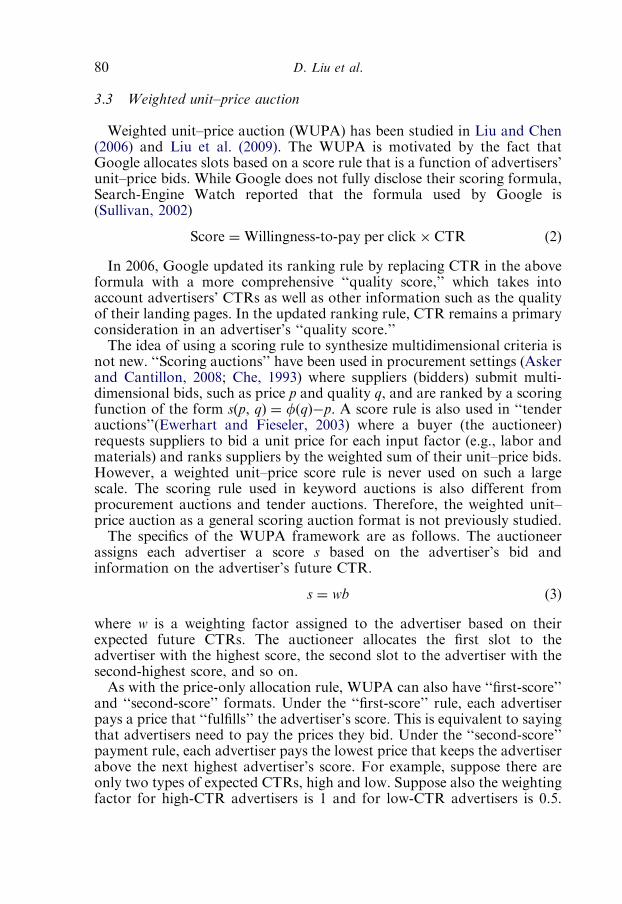
3.3 Weighted unit–price auction
Weighted unit–price auction (WUPA) has been studied in Liu and Chen(2006) and Liu et al. (2009). The WUPA is motivated by the fact thatGoogle allocates slots based on a score rule that is a function of advertisers’unit–price bids. While Google does not fully disclose their scoring formula,Search-Engine Watch reported that the formula used by Google is(Sullivan, 2002)
Score ¼Willingness-to-pay per click� CTR (2)
In 2006, Google updated its ranking rule by replacing CTR in the aboveformula with a more comprehensive ‘‘quality score,’’ which takes intoaccount advertisers’ CTRs as well as other information such as the qualityof their landing pages. In the updated ranking rule, CTR remains a primaryconsideration in an advertiser’s ‘‘quality score.’’The idea of using a scoring rule to synthesize multidimensional criteria is
not new. ‘‘Scoring auctions’’ have been used in procurement settings (Askerand Cantillon, 2008; Che, 1993) where suppliers (bidders) submit multi-dimensional bids, such as price p and quality q, and are ranked by a scoringfunction of the form s(p, q) ¼ f(q)�p. A score rule is also used in ‘‘tenderauctions’’(Ewerhart and Fieseler, 2003) where a buyer (the auctioneer)requests suppliers to bid a unit price for each input factor (e.g., labor andmaterials) and ranks suppliers by the weighted sum of their unit–price bids.However, a weighted unit–price score rule is never used on such a largescale. The scoring rule used in keyword auctions is also different fromprocurement auctions and tender auctions. Therefore, the weighted unit–price auction as a general scoring auction format is not previously studied.The specifics of the WUPA framework are as follows. The auctioneer
assigns each advertiser a score s based on the advertiser’s bid andinformation on the advertiser’s future CTR.
s ¼ wb (3)
where w is a weighting factor assigned to the advertiser based on theirexpected future CTRs. The auctioneer allocates the first slot to theadvertiser with the highest score, the second slot to the advertiser with thesecond-highest score, and so on.As with the price-only allocation rule, WUPA can also have ‘‘first-score’’
and ‘‘second-score’’ formats. Under the ‘‘first-score’’ rule, each advertiserpays a price that ‘‘fulfills’’ the advertiser’s score. This is equivalent to sayingthat advertisers need to pay the prices they bid. Under the ‘‘second-score’’payment rule, each advertiser pays the lowest price that keeps the advertiserabove the next highest advertiser’s score. For example, suppose there areonly two types of expected CTRs, high and low. Suppose also the weightingfactor for high-CTR advertisers is 1 and for low-CTR advertisers is 0.5.
D. Liu et al.80
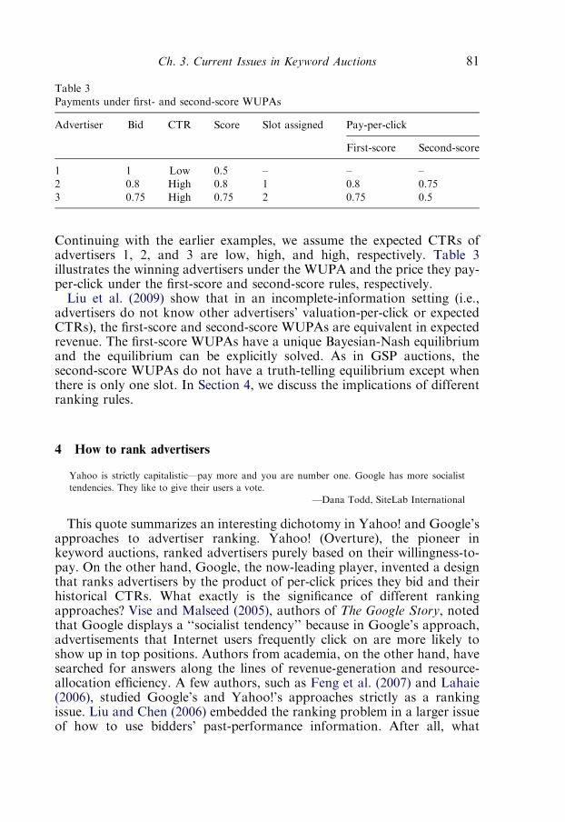
Continuing with the earlier examples, we assume the expected CTRs ofadvertisers 1, 2, and 3 are low, high, and high, respectively. Table 3illustrates the winning advertisers under the WUPA and the price they pay-per-click under the first-score and second-score rules, respectively.Liu et al. (2009) show that in an incomplete-information setting (i.e.,
advertisers do not know other advertisers’ valuation-per-click or expectedCTRs), the first-score and second-score WUPAs are equivalent in expectedrevenue. The first-score WUPAs have a unique Bayesian-Nash equilibriumand the equilibrium can be explicitly solved. As in GSP auctions, thesecond-score WUPAs do not have a truth-telling equilibrium except whenthere is only one slot. In Section 4, we discuss the implications of differentranking rules.
4 How to rank advertisers
Yahoo is strictly capitalistic—pay more and you are number one. Google has more socialist
tendencies. They like to give their users a vote.
—Dana Todd, SiteLab International
This quote summarizes an interesting dichotomy in Yahoo! and Google’sapproaches to advertiser ranking. Yahoo! (Overture), the pioneer inkeyword auctions, ranked advertisers purely based on their willingness-to-pay. On the other hand, Google, the now-leading player, invented a designthat ranks advertisers by the product of per-click prices they bid and theirhistorical CTRs. What exactly is the significance of different rankingapproaches? Vise and Malseed (2005), authors of The Google Story, notedthat Google displays a ‘‘socialist tendency’’ because in Google’s approach,advertisements that Internet users frequently click on are more likely toshow up in top positions. Authors from academia, on the other hand, havesearched for answers along the lines of revenue-generation and resource-allocation efficiency. A few authors, such as Feng et al. (2007) and Lahaie(2006), studied Google’s and Yahoo!’s approaches strictly as a rankingissue. Liu and Chen (2006) embedded the ranking problem in a larger issueof how to use bidders’ past-performance information. After all, what
Table 3
Payments under first- and second-score WUPAs
Advertiser Bid CTR Score Slot assigned Pay-per-click
First-score Second-score
1 1 Low 0.5 – – –
2 0.8 High 0.8 1 0.8 0.75
3 0.75 High 0.75 2 0.75 0.5
Ch. 3. Current Issues in Keyword Auctions 81
Google uses is the information on advertisers’ past CTRs, which essentiallysignals their abilities to generate clicks in the future. In fact, KAPs can alsoimpose differentiated minimum bids for advertisers of different historicalCTRs, which is what Google is doing now. This later use of past-performance information is studied in Liu et al. (2009).Three main questions are associated with different rank rules. What is the
impact of adopting different ranking rules on advertisers’ equilibriumbidding? On KAP’s revenue? And on resource-allocation efficiency? Therevenue and efficiency criteria may matter at different stages of the keywordadvertising industry. At the developing stage of the keyword advertisingmarket, it is often sensible for KAPs to use efficient designs to maximize the‘‘total pie.’’ After all, if advertisers see high returns from their initial use,they are likely to allocate more budgets to keyword advertising in thefuture. On the other hand, as the keyword advertising market matures andmarket shares stabilize, KAPs will more likely focus on revenue. Severalauthors in economics, information systems, and computer science haveapproached these questions.Feng et al. (2007) are the earliest to formally compare the ranking rules of
Google and Yahoo! One focus of their study is the correlation betweenadvertisers’ pay-per-click and the relevance of their advertisements to thekeywords. With numerical simulation, they find that Google’s rankingmechanism performs well and robustly across varying degrees of correla-tion, while Yahoo!’s performs well only if pay-per-click and relevance arepositively correlated. Those observations are sensible. Intuitively, anadvertiser’s contribution to the KAP’s revenue is jointly determined bythe advertiser’s pay-per-click and the number of clicks the advertiser cangenerate (i.e., relevance). When pay-per-click is negatively correlated withrelevance, ranking purely based on pay-per-click tends to select advertiserswith low revenue contribution, which can result in a revenue loss for KAPs.However, their study has certain limitations. Instead of solving the auctionmodel, they simplify by assuming that bidders will bid truthfully underGoogle’s mechanism.Lahaie (2006) compares Google’s and Yahoo!’s ranking rules based on an
explicit solution to the auction-theoretic model. He finds that Google’sranking rule is efficient while Yahoo!’s is not. Yahoo!’s ranking is inefficientbecause, as we mentioned earlier, high bid does not necessarily meanhigh total valuation because total valuation also depends on relevance.In contrast, Google’s ranking rule is efficient. He also shows that norevenue ranking of Google’s and Yahoo!’s ranking mechanism is possiblegiven an arbitrary distribution over bidder values and relevance. Hisfindings are consistent with results derived in a weighted unit–price auctionframework by Liu and Chen (2006) and Liu et al. (2009), which we discussnext.While both Feng et al. (2007) and Lahaie (2006) focus on two specific
cases: Yahoo!’s price-only ranking rule and Google’s ranking rule, Liu
D. Liu et al.82

and Chen (2006) and Liu et al. (2009) study weighted unit–priceauctions (WUPAs), which encompass Yahoo! and Google’s ranking rules.Under WUPAs, advertisers bid on their willingness-to-pay per click (orunit–price), and the auctioneer weighs unit–price bids based on advertisers’expected CTRs. Liu and Chen (2006) consider a single slot setting. Liu et al.(2009) extend to a more general multiple slot setting and study both rankingrules and minimum-bid rules.As in Section 3, advertiser i, if assigned to slot j, will generate cij ¼ djqi
clicks, where dj is a deterministic coefficient that captures the prominence ofslot j. d1X d2 . . . X dm and d1 ¼ 1. qi is a stochastic number that capturesthe advertiser i’s CTR.A key assumption of the WUPA framework is that the KAP has
information on advertisers’ future CTRs. This assumption is motivated by thefact that e-commerce technologies allow KAPs to track advertisers’ pastCTRs and predict their future CTRs. The KAP can make the ranking ofadvertisers depend on both their pay-per-click and their expected CTRs. Inparticular, the KAP assigns each advertiser a score s ¼ wb, where theweighting factor w is determined by the advertiser’s expected CTR. Ifthe advertiser has high-expected CTR, then the weighting factor is 1. If theadvertiser has low expected CTR, then the weighting factor is wl.Liu et al. (2009) study WUPAs in an incomplete information setting. They
assume that each advertiser has a private valuation-per-click v, v 2 ½v; �v �.The distributions of valuation-per-click, Fh(v) (for high-CTR advertisers)and Fl(v) (for low-CTR advertisers), are known to all advertisers and theKAP. The probabilities of being a high-CTR advertiser, a, and a low-CTRone, 1�a, are also known to all advertisers and the KAP. Furthermore, wedenote Qh and Ql as the expected CTRs for a high-CTR advertiser and alow-CTR advertiser, respectively. It is assumed that QhWQl.Suppose advertisers’ payoff functions are additive in their total valuation
and the payment. Under the first-score payment rule (see Section 3),3 thepayoffs for a low-CTR advertiser and a high-CTR advertiser are, respectively,
Ulðv; bÞ ¼ Qlðv� bÞXmj¼1
djPrfwlb ranks jthg (4)
Uhðv; bÞ ¼ Qhðv� bÞXmj¼1
djPrfb ranks jthg (5)
Liu et al.’s analysis generates several insights. First, their analysisillustrates how ranking rules affects equilibrium bidding. The ranking ruleaffects how low- and high-CTR advertisers match up against each other inequilibrium. Specifically, weighting factors for low- and high-CTR
3In this model setting, a first-score auction is revenue-equivalent to a second-score auction.
Ch. 3. Current Issues in Keyword Auctions 83
advertisers determine the ratio of valuation-per-clicks between a low-CTRadvertiser and a high-CTR advertiser who tie in equilibrium. For example,if the low-CTR advertisers are given a weighting factor of 0.6, and the high-CTR advertiser, 1, a low-CTR advertiser with valuation-per-click 1 will tiewith a high-CTR advertiser with valuation-per-click 0.6 in equilibrium.Furthermore, high-CTR advertisers’ with valuation-per-click higher than0.6 out-compete all the low-CTR advertisers, and therefore compete onlywith other high-CTR competitors. As a result, these high-CTR advertiserswill bid markedly less aggressively than high-CTR advertisers withvaluation-per-click lower than 0.6.Second, they identify the efficient ranking rule under the WUPA
framework. Here efficiency is measured by the total expected valuationrealized in the auction. The efficient ranking rule under the WUPAframework is remarkably simple: The KAP should weigh advertisers’pay-per-click by their expected CTRs, as if they bid their true valuation-per-click (while in fact they generally do not).Third, they characterize the revenue-maximizing ranking rule under the
WUPAs. The revenue-maximizing ranking rule may favor low- or high-CTR advertisers relative to the efficient ranking rule. When the distributionof valuation-per-click is the same for high- and low-CTR advertisers, therevenue-maximizing ranking rule should always favor low-CTR advertisers(relative to the efficient design). But when the valuation distribution of low-CTR advertisers become less ‘‘disadvantaged,’’ the revenue-maximizingranking rule may instead favor high-CTR advertisers (relative to theefficient design).Besides the above-mentioned research on ranking rules, Weber and
Zheng (2007) study the revenue-maximizing ranking rule in a setting thatresembles ‘‘paid placement.’’ They study a model where two competingfirms can reach their customers through sponsored links offered by a searchengine intermediary. Consumers differ in ‘‘inspection cost’’ (cost incurredwhen they click on a sponsored link to find out the surplus they can getfrom purchasing the product). Thus, some consumers may inspect only thefirst link, while others inspect both before making a purchase decision. Toget the higher position, firms can offer a payment b to the search engineeach time a consumer clicks on their product link (their ‘‘bids’’). The searchengine’s problem is to choose how to rank the firms, given the consumersurplus u generated by two firms (assumed known to the search engine) andtheir bids b. The authors study an additive ranking rule
sðb; u;bÞ ¼ buþ ð1� bÞb (6)
where the parameter b is the focal design factor. They find that the revenue-maximizing ranking design should put nonzero weight on firms’ bid b. Inother words, search engines have incentive to accept ‘‘bribes’’ fromadvertisers to bias the ranking of product links.
D. Liu et al.84
5 How to package resources
Keyword auctions maintain that bidders simply bid their willingness-to-pay per click (thousand-impression, action) and are assigned to slots by anautomatic algorithm, with higher-ranked advertisers receiving a better slot(more exposure). This is different from a fixed-price scheme, where sellersspecify a menu of price-quantity pairs for buyers to choose from, and fromtraditional divisible-good auctions where sellers need not specify anythingand buyers bid both price and quantity they desire. In a sense, keywordauctions strike a middle ground between the fixed-price scheme andtraditional divisible-good auctions: in keyword auctions, the buyers(advertisers) specify prices they desire, and the seller (the KAP) decidesthe quantities to offer. Given the unique division of tasks in keywordauction settings, how to package resources for auctioning becomes animportant issue facing KAPs.Before we address the issue of resource packaging, it is useful to clarify
what we mean by resource in keyword auctions and why resourcepackaging is a practical issue. What KAPs sell to advertisers is impressions.Each time a page is requested by an Internet user, all advertisements on thispage get an impression. Though keyword advertising is often priced by thenumber of clicks or ‘‘actions’’ (e.g., purchases), KAPs can always re-allocate impressions from one advertiser to another but cannot do the samewith clicks or actions. Therefore, impression is the ultimate resourcecontrolled by KAPs.Although slots on the same page generate the same number of
impressions, they may not be equal to advertisers. For example, anadvertising slot is noticed more often if it is at the top of a page than atthe bottom of the page. Other factors can also affect how often a slot isnoticed, such as its geometric size, the time of the day it is displayed, andwhether the deployment website is frequented by shoppers. One way toaddress these differences in page impressions is to substitute rawimpressions with standardized effective exposure, which weighs impressionsdifferently based on how much value it can deliver to an average advertiser.For example, if the effective exposure generated by one page impressionat the top of a page is 1, then the effective exposure, generated by onepage impression at the bottom of the page might be 0.3. In the followingwe study the packaging of effective exposures rather than raw pageimpressions.4
With the notion of effective exposure, a keyword auction goes like this.The KAP packages the available effective exposure into several shares,
4A recommendation based on effective exposure can be transparently translated into a recommenda-tion based on raw page impressions. This is because KAPs can always tailor the exposure allocated to anadvertisement by randomizing its placement between different slots, varying the timing and length of itsappearance, and/or selecting the number of websites for the advertisement to appear.
Ch. 3. Current Issues in Keyword Auctions 85

ordered from large to small. Advertisers will be assigned to shares by theirrankings, with the highest-ranked advertiser receiving the largest share, thesecond-highest-ranked advertiser receiving the second-largest share, and soon. A resource packaging problem in such a setting is to decide how manyshares to provide and the size of each share to maximize total revenues. Wecall this problem a share-structure design problem.The share-structure design problem is relevant to KAP’s day-to-day
operations. The demand and supply of keyword advertising resources arehighly dynamic. On one hand, the supply of advertising resources fluctuatesas new websites join KAPs’ advertising network, and existing websites maylose their draw of online users. On the other hand, the demand foradvertising on particular keywords shifts constantly in response to changesin underlying market trends. Therefore, KAPs must constantly adjust theirshare structures to maximize their total revenue. To do so, KAPs need agood understanding of the share structure design problem. Given thatKAPs have become managers of tremendous advertising resources, theissue of share structure design is critical to their success.
5.1 The revenue-maximizing share structure problem
Chen et al. (2006, 2009) address the issue of revenue-maximizing sharestructures with the following specifications. There are n risk-neutraladvertisers (bidders). The KAP (auctioneer) packages total effectiveexposure (normalized to 1) into as many as n shares arranged in adescending order, s1 � s2 � � � � � sn. A share structure refers to vectors ¼ (s1, s2, . . . sn). Table 4 shows some examples of share structures andtheir interpretations.Bidders’ valuation for a share is determined by the size of the share (s)
and a private parameter (v), called the bidder’s type. v is distributedaccording to a cumulative distribution function F(v) on ½ v; �v �, with densityf(v). Bidders’ valuation of a share take the form of vQ(s), where Q(d) is anincreasing function.Bidders are invited to bid their willingness-to-pay per unit exposure (or
unit price), and all shares are allocated at once by a rank-order of bidders’unit–price bids.5 Bidders pay the price they bid.6 Each bidder’s expectedpayoff is the expected valuation minus expected payment to the auctioneer.Denote pj(b) as the probability of winning share j by placing bid b. The
5Google ranks advertisers by a product of their willingness-to-pay per click and a click-through-rate-based quality score, which can be loosely interpreted as advertisers’ willingness-to-pay per impression(see Liu and Chen (2006) for a more detailed discussion). Yahoo! used to rank advertisers by theirwillingness-to-pay per click only, but recently switched to a format similar to Google’s. Our assumptionthat bidders are ranked by their willingness-to-pay per unit exposure is consistent with both Google’sapproach and Yahoo!’s new approach.
6The expected revenue for the auctioneer is the same if bidders pay the next highest bidder’s price.
D. Liu et al.86

expected payoff of a bidder of type v is
Uðv; bÞ ¼Xnj¼1
pjðbÞðvQðsjÞ � bsjÞ (7)
The auctioneer’s revenue is expected total payments from all bidders.
p ¼ nE bXnj¼1
pjðbÞsj
" #(8)
Bidders maximize their expected payoff by choosing a unit price b.The auctioneer maximizes the expected revenue by choosing a sharestructure s.
5.2 Results on revenue-maximizing share structures
Chen et al. (2009) showed that the auctioneer’s expected revenue in theabove setting is written as
p ¼ nXnj¼1
QðsjÞ
Z �v
v
PjðvÞ v�1� FðvÞ
f ðvÞ
� �f ðvÞdv (9)
where
PjðvÞ �n� 1
n� j
!FðvÞn�jð1� FðvÞÞ j�1 (10)
is the equilibrium probability for a bidder of type v to win share j.We denote
aj � n
Z �v
v
PjðvÞ v�1� FðvÞ
f ðvÞ
� �f ðvÞdv; j ¼ 1; 2; . . . ; n (11)
Table 4
Examples of share structures
s Interpretation
(1, 0, 0, 0) The highest bidder gets all effective exposures
(0.25, 0.25, 0.25, 0.25) Top 4 bidders each get one-fourth of the total effective exposures
(0.4, 0.2, 0.2, 0.2) The top bidder gets 40% of the total effective exposures. The
2nd–4th highest bidders each get 20% of the total effective
exposures
Ch. 3. Current Issues in Keyword Auctions 87

The expected revenue (Eq. (9)) can be written as
p ¼Xnj¼1
ajQðsjÞ (12)
Here aj is interpreted as the return coefficient for the jth share.Chen et al. (2009) showed that the revenue-maximizing share structures
may consists of plateaus—a plateau is a set of consecutively ranked shareswith the same size. For example, the third example in Table 4 has twoplateaus: the first plateau consists of the first share (of size 0.4); the secondplateau consists of the second to the fourth share (of size 0.2). Chen et al.(2009) showed that the starting and ending ranks of plateaus in the revenue-maximizing share structure are determined only by the distribution ofbidders’ type. Based on their analysis, the optimal starting/ending ranks ofplateaus and the optimal sizes of shares in each plateau can be computedusing the following algorithm.
1. Compute return coefficients {aj }, j ¼ 1, . . . ,n.2. Let jk denote the ending rank of k-th plateau. j0 ( 0 and k( 1.3. Given jk�1, compute jk ( argmaxj2fjk�1þ1;...;ngfð1=ð j � jk�1ÞÞ
Pjl¼jk�1þ1
alg.4. If jk ¼ n, K ( k (K denotes the total number of plateaus) and
continue to step 5. Otherwise, k( kþ 1, go to step 3.5. Compute the average return coefficient �ak ( ð1=ðjk � jk�1ÞÞPjk
l¼jk�1þ1al, for plateau k ¼ 1, . . . , K.
6. Solve the following nonlinear programming problem for the sizes ofshares (z1, z2, . . . ,zK) in all plateaus:
maxXKk¼1
ð jk � jk�1Þ�akQðzkÞ
subject to :XKk¼1
ð jk � jk�1Þzk ¼ 1 and z1 � z2 � � � � � zK � 0
A share structure becomes steeper if we allocate more resources to high-ranked shares and less to low-ranked ones. In Table 4, the steepest sharestructure is (1, 0, 0, 0), followed by (0.4, 0.2, 0.2, 0.2), and then by (0.25,0.25, 0.25, 0.25). Chen et al. (2009) obtained several results on how therevenue-maximizing share structures should change in steepness when theunderlying demand or supply factors change. First, as bidders’ demandsbecome less price-elastic (as the valuation function Q(d) becomes moreconcave), the auctioneer should use a less steep share structure. Whenbidders have perfectly elastic demand (i.e., the bidder’s valuation Q(d) is a
D. Liu et al.88
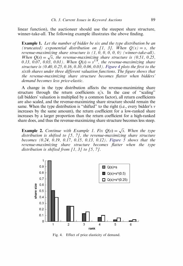
linear function), the auctioneer should use the steepest share structure,winner-take-all. The following example illustrates the above finding.
Example 1. Let the number of bidder be six and the type distribution be an(truncated) exponential distribution on [1, 3]. When Q(s) ¼ s, therevenue-maximizing share structure is (1, 0, 0, 0, 0, 0) (winner-take-all).When QðsÞ ¼
ffiffisp
, the revenue-maximizing share structure is (0.51, 0.25,0.13, 0.07, 0.03, 0.01). When Q(s) ¼ s1/4, the revenue-maximizing sharestructure is (0.40, 0.25, 0.16, 0.10, 0.06, 0.03). Figure 4 plots the first to thesixth shares under three different valuation functions. The figure shows thatthe revenue-maximizing share structure becomes flatter when bidders’demand becomes less price-elastic.
A change in the type distribution affects the revenue-maximizing sharestructure through the return coefficients aj’s. In the case of ‘‘scaling’’(all bidders’ valuation is multiplied by a common factor), all return coefficientsare also scaled, and the revenue-maximizing share structure should remain thesame. When the type distribution is ‘‘shifted’’ to the right (i.e., every bidder’s vincreases by the same amount), the return coefficient for a low-ranked shareincreases by a larger proportion than the return coefficient for a high-rankedshare does, and thus the revenue-maximizing share structure becomes less steep.
Example 2. Continue with Example 1. Fix QðsÞ ¼ffiffisp
. When the typedistribution is shifted to [5, 7], the revenue-maximizing share structurebecomes (0.24, 0.19, 0.17, 0.15, 0.13, 0.12). Figure 5 shows that therevenue-maximizing share structure becomes flatter when the typedistribution is shifted from [1, 3] to [5, 7].
Fig. 4. Effect of price elasticity of demand.
Ch. 3. Current Issues in Keyword Auctions 89

Another factor studied in Chen et al. (2009) is the effect of increasingtotal resources available. They showed that when total resource increases,all shares will increase, but whether the share structure (in terms ofpercentages of the total resources) becomes flatter or steeper depends onhow bidders price elasticity increases or decreases with the resourcesassigned. When bidders’ price elasticity increases in the amount of resourcesallocated, the KAP should increase high-ranked shares by a largerpercentage. When bidders’ price elasticity of demand decreases, the KAPshould increase low-ranked shares by a larger percentage.The above results highlighted the importance of advertisers’ price
elasticity of demand and the competitive landscape (as determined bythe distribution of bidders’ types). Generally speaking, when biddersbecome more price-elastic, the share structure should be steeper; whenthe competition between bidders is fiercer, the share structure should beflatter.
5.3 Other issues on resource packaging
The resources managed by KAPs have expanded significantly since theadvent of keyword advertising. Leading KAPs have developed vastadvertising networks of thousands of websites. Meanwhile, they are alsoactively seeking expansion to other media, including mobile devices, radio,and print advertising. The issue of resource packaging will only becomemore important when KAPs manages more advertising resources.
Fig. 5. Effect of type distribution.
D. Liu et al.90
The earlier research addressed only a small part of a larger resource-packaging problem. There are a few interesting directions for futureresearch on the issue of resource packaging. First, Chen et al.’s (2009)framework assumes bidders share a common valuation function Q. A moregeneral setting is that bidders’ valuation functions are also different. Forexample, bidders with highly elastic demand and bidders with inelasticdemands may coexist. Feng (2008) studies a setting in which bidders differin price elasticities, but her focus is not on the share structure design.Another interesting direction is to compare keyword auctions with
alternative mechanisms for divisible goods such as the conventionaldiscriminatory-price and uniform-price auctions (Wang and Zender, 2002;Wilson, 1979), in which bidders not only bid on prices but also on thequantity desired. The study on revenue-maximizing share structurefacilitates such comparison because one would need to pick a revenue-maximizing share structure for keyword auctions to make a meaningfulcomparison.Also, it is interesting to study the optimal mechanism for allocating
keyword-advertising resources. Different mechanisms may be evaluatedalong the lines of the auctioneer’s revenue, the allocation efficiency, andwhether the mechanism encourages bidders to reveal their true valuation.Bapna and Weber (2006) study a mechanism that allows bidders to specifytheir ‘‘demand curves,’’ rather than just one price. They consider a moregeneral setting in which multiple divisible goods are offered and biddersmay have multidimensional private information. More specifically, theyconsider n bidders that have valuation for fractional allocations of m slots.For a fraction xi ¼ ðx
1i ; . . . ; x
mi Þ allocated, bidder i’s utility is vi (xi;Zi),
where Zi represents bidder i’s private information, or type. The auctioneerfirst announces its mechanism, which includes a fixed m-dimensional pricevector p ¼ (p1, . . . , pm). Then each bidder submits a bid function bi(d; Zi).The bidder’s bids are considered as discounts that will be subtracted fromthe payment implied by the posted price schedule. Under such a setting,Bapna and Weber show that such a mechanism has a dominant-strategyincentive-compatible equilibrium in which a bidder’s equilibrium bids donot depend on the knowledge of type distribution, the number of bidders,or other bidders’ payoff functions.
6 Click fraud
The keyword advertising industry has been extraordinarily successful inthe past few years and continues to grow rapidly. However, its core ‘‘pay-per-click’’ advertising model faces a threat known as ‘‘click fraud.’’ Clickfraud occurs when a person, automated script, or computer programimitates a legitimate user of a web browser clicking on an advertisement, forthe purpose of generating a click with no real interest in the target link. The
Ch. 3. Current Issues in Keyword Auctions 91

consequences of click fraud include depleting advertisers’ budgets withoutgenerating any real returns, increasing uncertainties in the cost ofadvertising campaigns, and creating difficulty in estimating the impact ofkeyword advertising campaigns. Click fraud can ultimately harm KAPsbecause advertisers can lose confidence in keyword advertising and switchto other advertising outlets. Both industrial analysts and KAPs have citedclick fraud as a serious threat to the industry. A Microsoft AdCenterspokesperson stated, ‘‘Microsoft recognizes that invalid clicks, whichinclude clicks sometimes referred to as ‘click fraud,’ are a serious issue forpay-per-click advertising.’’7 In its IPO document, Google warned that ‘‘weare exposed to the risk of fraudulent clicks on our ads.’’8 While noconsensus exists on how click fraud should be measured, ‘‘most academicsand consultants who study online advertising estimate that 10% to 15% ofadvertisement clicks are fake, representing roughly $1 billion in annualbillings’’ (Grow and Elgin, 2006).Click fraud has created a lingering tension between KAPs and
advertisers. Because advertisers pay for valid click they receive, it is criticalfor advertisers not to pay for clicks that are invalid or fraudulent. Thetension arises when advertisers and KAPs cannot agree on which clicks arevalid. KAPs often do not inform advertisers which clicks are fraudulentclicks, citing the concern that click spammers may use such informationagainst KAPs and undermine KAPs’ effort to fight click fraud. Also, KAPsmay have financial incentives to charge advertisers for invalid clicks toincrease their revenues. Such incentives may exist at least in a short run. Afew events illustrate the tension between advertisers and KAPs. In June2005, Yahoo! settled a click-fraud lawsuit and agreed to pay the plaintiffs’$5 million legal bills. In July 2006, Google settled a class-action lawsuit overalleged click fraud by offering a maximum of $90 million credits tomarketers who claim they were charged for invalid clicks.Before we proceed, it is useful to clarify the two main sources of
fraudulent clicks. The first is from competing advertisers. Knowing thatmost advertisers have a daily spending budget, an advertiser can initiate aclick-fraud attack on competitors to drain their daily budgets. Once thecompetitors’ daily budgets are exhausted, their advertisements will besuspended for the rest of the day, so the attacker can snag a high rank atless cost.The second and more prevalent source of click fraud comes from
publishers who partner with KAPs to display keyword advertisements.Many publishers earn revenue from KAPs on a per-click basis. Therefore,they have incentives to inflate the number of clicks on the advertisementsdisplayed on their sites. This became a major form of click fraud afterKAPs expanded keyword advertising services to millions of websites,
7http://news.com.com/2100-10243-6090939.html8http://googleblog.blogspot.com/2006/07/let-click-fraud-happen-uh-no.html
D. Liu et al.92

including many small and obscure websites that are often built solely foradvertising purposes.One argument is that click fraud is not a real threat. This line of argument
underlines current Google CEO Eric Schmidt’s comment on click fraud.9
Let’s imagine for purposes of argument that click fraud were not policed by Google and it were
rampant . . . Eventually, the price that the advertiser is willing to pay for the conversion will
decline, because the advertiser will realize that these are bad clicks, in other words, the value of
the ad declines, so over some amount of time, the system is in fact self-correcting. In fact, there is
a perfect economic solution which is to let it happen.
Research also shows that Google’s keyword auction mechanisms resistclick fraud (Immorlica et al., 2005; Liu and Chen, 2006). The reason is thatadvertisers who suffer from click fraud also gain in their CTR rating, whichworks in their favor in future auctions (recall that Google’s rankingmechanism favors advertisers with high historical CTRs).While the above arguments have merits, they also have flaws. The first
argument works best when the click-fraud attack is predictable. When theattack is unpredictable, advertisers cannot effectively discount its impact.Also, unpredictable click fraud creates uncertainties for advertisers, whichcan make keyword advertising unattractive. As to the second argument,while receiving fraudulent clicks has positive effects under the current system,it is unclear whether the positive effects can dominate the negative ones.In what follows, we discuss measures to detect and to prevent click fraud.
Detection efforts such as online filtering and off-line detection reduce thenegative impact of fraudulent clicks. Preventive measures such as usingalternative pricing or a new rental approach can reduce or eliminateincentives to conduct click fraud.
6.1 Detection
6.1.1 Online filteringA major tool used in combating click fraud is an automatic algorithm
called ‘‘filter.’’ Before charging the advertisers, major KAPs use automaticfilter programs to discount suspected fraudulent clicks as they occur. Suchfilters are usually rule-based. For example, if a second click on theadvertisement occurs immediately after a first click, the second click (‘‘thedoubleclick’’) is automatically marked as invalid, and the advertiser will notpay for it. KAPs may deploy multiple filters so that if one filter misses afraudulent click, another may still have a chance to catch it. Tuzhilin (2006)studied filters used by Google and stated that Google’s effort in filtering outinvalid clicks is reasonable, especially after Google started to considerdoubleclicks as invalid clicks in 2005.
9http://googleblog.blogspot.com/2006/07/let-click-fraud-happen-uh-no.html
Ch. 3. Current Issues in Keyword Auctions 93

While some fraudulent clicks are easy to detect (e.g., doubleclicks), othersare very difficult. For example, it is virtually impossible to determinewhether a click is made by a legitimate Internet user or by a laborer hiredcheaply in India to click on competitors’ advertisements.10 The currentfilters are still simplistic (Tuzhilin, 2006). More sophisticated and time-consuming methods are not used in online filters because they do not workwell in real-time. As a result, current filters may miss sophisticated and less-common attacks (Tuzhilin, 2006). The fact that advertisers have requestedrefunds or even pursued lawsuits over click fraud indicates that filterprograms alone cannot satisfyingly address the click fraud problem.
6.1.2 Off-line detectionOff-line detection methods do not have the real-time constraint.
Therefore an off-line detection team can deploy more computationallyextensive methods, and consider a larger set of clicking data and manyother factors (such as conversion data). Off-line detection can be automaticor manual. Google uses automated off-line detection methods to generatefraud alerts and to terminate publishers’ accounts for fraudulent clickpatterns. Automatic off-line detection methods are pre-programmed; thusthey cannot react to new fraud patterns. Google also uses manual off-linedetection to inspect click data questioned by advertisers, alert programs, orinternal employees. While such manual detection is powerful, it is hardlyscalable. Unlike online filtering, off-line detection does not automaticallycredit advertisers for invalid clicks. However, if a case of click fraud isfound, advertisers will be refunded.
6.2 Prevention
First of all, KAPs may prevent click fraud by increasing the cost ofconducting click fraud. KAPs have taken several other steps in discoura-ging click spammers, including (Tuzhilin, 2006):
� Making it hard for publishers to create duplicate accounts or open newaccounts after the old accounts are terminated,� Making it hard for publishers to register using false identities, and� Automatically discounting fraudulent clicks so that click spammers arediscouraged.
All of the above prevention efforts rely on a powerful click-frauddetection system. However, a powerful and scalable click-fraud system isvery difficult, if not impossible, to develop. The above prevention efforts aredwarfed if sophisticated click spammers can pass the detection.
10http://timesofindia.indiatimes.com/articleshow/msid-654822,curpg-1.cms
D. Liu et al.94

6.2.1 Alternative pricingPay-per-click is susceptible to click fraud because clicks can be easily
falsified. Witnessing this, some suggest different pricing metrics, such aspay-per-action (e.g., pay-per-call and pay-per-purchase), as a remedy toclick fraud. Because purchases and calls are much more costly to falsify,switching to a pay-per-action or pay-per-call pricing scheme will overcomethe click-fraud problem.Pay-per-action pricing is unlikely a remedy for all advertisers. Sometimes
outcome events such as purchases are hard to track or define (e.g., shouldKAPs count a purchase if it is made the next day after the customer visitedthe link?). Other times, advertisers may be reluctant to share purchaseinformation with KAPs. Finally, different advertisers may be interested indifferent outcome measures. For example, direct marketers are moreinterested in sales, while brand advertisers may be interested in the timeInternet users spend on their websites.One may suggest going back to the pay-per-impression model to prevent
click fraud. However, pay-per-impression is subject to fraud of its ownkind: knowing that advertisers are charged on per-impression basis, amalicious attacker can request the advertising pages many times to exhaustthe advertisers’ budgets; similarly, publishers can recruit viewers to theirwebsites to demand higher revenue from KAPs. Goodman (2005) proposeda pricing scheme based on percentage of impressions. The assumption isthat if attackers systematically inflate impressions, advertisers will pay thesame amount because they still receive the same percentage of allimpressions. While this proposed pricing scheme addresses the click-fraudproblem to a large extent, it also has some consequences. For example, sucha pricing scheme will not automatically adjust to the changes in overalllegitimate traffic. As a result, web publishers have no incentives to increasethe popularity of their websites. Also, the pay-per-percentage-impressionpricing imposes all risks on advertisers. In general, advertisers are morerisk-averse than KAPs, and it is often revenue-maximizing for KAPs toabsorb some of the risks.
6.2.2 Rental modelAnother possible remedy is a rental model in which advertisers bid on
how much they are willing to pay per hour exposure. Clearly, such a pricingmodel is immune to the click-fraud problem. The rental model can beimplemented in different ways. One way is to ask each advertiser to bid oneach slot, and KAPs will assign the slot to the highest bidder. Alternatively,KAP can ask advertisers to bid on the first slot only, provided that theyagree on receiving other slots at a discounted price proportional to their bidfor the first slot. Such a rental model can be valuable when advertisers havea reasonable idea about how much exposure they can get from a particularslot. Of course, when the outcome is highly uncertain, a rental model alsoexposes advertisers to grave risks.
Ch. 3. Current Issues in Keyword Auctions 95
In sum, a single best solution to the click-fraud problem may not exist.While alternatives to pay-per-click advertising may remove incentives toconduct click fraud, they often come with other costs and limitations.Clearly, future keyword auction designs must take into account the click-fraud problem.
7 Concluding remarks
In this chapter, we review the current research on keyword advertisingauctions. Our emphasis is on keyword-auction design. Keyword auctionsare born out of practice and have unique features that previous literaturehas not studied. Keyword auctions are still evolving, giving us anopportunity to influence future keyword-auction designs. Given the centralposition of search and advertising in online worlds, research on keywordauctions holds important practical values.It is worth noting that keyword auctions as a mechanism for allocating
massive resources in real-time are not limited to online advertising settings.Other promising areas of application of keyword auctions includegrid-computing resources, Internet bandwidth, electricity, radio spectrum,and some procurement areas. In fact, Google filed a proposal on May 21,2007, to the Federal Communications Commission calling on usingkeyword-auction-like mechanisms to allocate radio spectrum. In theproposal, Google argued that a keyword-auction-like real-time mechanismwould improve the fairness and efficiency of spectrum allocation and createa market for innovative digital services. As keyword auctions as a generalmechanism are proposed and tested in other settings, several importantquestions arise. For example, what conditions are required for keywordauctions to perform well? And what needs to be changed for keywordauctions to apply in new settings?This chapter focuses on design issues within keyword advertising settings.
It would also be interesting to compare keyword auctions with various otheralternative mechanisms in different settings. It is not immediately clearwhether keyword auctions are superior to, for instance, dynamic pricing ora uniform-price auction where bidders bid both price and quantity. Moreresearch must be done to integrate the brand-new keyword auctions into theexisting auction literature. We believe research in such a direction will yieldnew theoretical insights and contribute to the existing auction literature.
References
Asdemir, K. (2005). Bidding Patterns in Search Engine Auctions, Working Paper, University of Alberta
School of Business.
D. Liu et al.96

Asker, J.W., E. Cantillon (2008). Properties of Scoring Auctions. RAND Journal of Economics 39(1),
69–85.
Bapna, A., T.A. Weber (2006). Efficient Allocation of Online Advertising Resources, Working Paper,
Stanford University.
Che, Y.-K. (1993). Design competition through multidimensional auctions. Rand Journal of Economics
24(4), 668–680.
Chen, J., D. Liu, A.B. Whinston (2006). Resource packaging in keyword auctions, in: Proceedings of the
27th International Conference on Information Systems, December, Milwaukee, WI, pp. 1999–2013.
Chen, J., D. Liu, A.B. Whinston (2009). Auctioning keywords in online search. Forthcoming in Journal
of Marketing.
Edelman, B., M. Ostrovsky, M. Schwarz (2007). Internet advertising and the generalized second price
auction: Selling billions of dollars worth of keywords. American Economic Review 97(1), 242–259.
eMarketer (2007). Online advertising on a rocket ride. eMarketer News Report, November 7.
Ewerhart, C., K. Fieseler (2003). Procurement auctions and unit-price contracts. Rand Journal of
Economics 34(3), 569–581.
Feng, J. (2008). Optimal mechanism for selling a set of commonly ranked objects. Marketing Science
27(3), 501–512.
Feng, J., H. Bhargava, D. Pennock (2007). Implementing sponsored search in web search engines:
Computational evaluation of alternative mechanisms. INFORMS Journal on Computing 19(1),
137–148.
Goodman, J. (2005). Pay-per-percentage of impressions: An advertising method that is highly robust to
fraud. Workshop on Sponsored Search Auctions, Vancouver, BC, Canada.
Grow, B., B. Elgin (2006). Click fraud: The dark side of online advertising. Business Week, October 2.
Immorlica, N., K. Jain, M. Mahdian, K. Talwar (2005). Click Fraud Resistant Methods for Learning
Click-Through Rates. Workshop for Internet and Network Economics.
Interactive Advertising Bureau. (2007). Internet advertising revenues grow 35% in ’06, hitting a record
close to $17 billion. Interactive Advertising Bureau News Press Release, May 23.
Lahaie, S. (2006). An analysis of alternative slot auction designs for sponsored search, in: Proceedings of
the 7th ACM Conference on Electronic Commerce, Ann Arbor, MI, ACM Press.
Liu, D., J. Chen (2006). Designing online auctions with performance information. Decision Support
Systems 42(3), 1307–1320.
Liu, D., J. Chen, A.B. Whinston (2009). Ex-Ante Information and the Design of Keyword Auctions.
Forthcoming in Information Systems Research.
Sullivan, D. (2002). Up close with Google Adwords. Search Engine Watch Report.
Tuzhilin, A. (2006). The Lane’s Gifts v. Google Report. Available at http://googleblog.blogspot.com/
pdf/TuzhilinReport.pdf. Retrieved on December 25, 2007.
Varian, H.R. (2007). Position auctions. International Journal of Industrial Organization 25(6), 1163–1178.
Vise, A.D., M. Malseed (2005). The Google story. New York, NY.
Wang, J.J.D., J.F. Zender (2002). Auctioning divisible goods. Economic Theory 19(4), 673–705.
Weber, T.A., Z. Zheng (2007). A model of search intermediaries and paid referrals. Information Systems
Research 18(4), 414–436.
Wilson, R. (1979). Auctions of shares. The Quarterly Journal of Economics 93(4), 675–689.
Zhang, X., J. Feng (2005). Price cycles in online advertising auctions, in: Proceedings of the 26th
International Conference on Information Systems, December, Las Vegas, NV, pp. 769–781.
Ch. 3. Current Issues in Keyword Auctions 97

This page intentionally left blank
Adomavicius & Gupta, Eds., Handbooks in Information Systems, Vol. 3
Copyright r 2009 by Emerald Group Publishing Limited
Chapter 4
Web Clickstream Data and Pattern Discovery:A Framework and Applications
Balaji PadmanabhanInformation Systems and Decision Sciences Department, College of Business, University of
South Florida, 4202 E. Fowler Avenue, CIS 1040, Tampa, FL 33620, USA
Abstract
There is tremendous potential for firms to make effective use of Webclickstream data. In a perfect world a firm will be able to optimally manageonline customer interactions by using real-time Web clickstream data. Here itmay be possible to proactively serve users by determining customer interestsand needs before they are even expressed. Effective techniques for learningfrom this data are needed to bridge the gap between the potential inherent inclickstream data and the goal of optimized customer interactions. Techniquesdeveloped in various fields including statistics, machine learning, databases,artificial intelligence, information systems and bioinformatics can be of valuehere, and indeed several pattern discovery techniques have been proposed inthese areas in the recent past. In this chapter we discuss a few applications ofpattern discovery in Web clickstream data in the context of a new patterndiscovery framework presented here. The framework is general and we noteother applications and opportunities for research that this framework suggests.
1 Background
From a business perspective the Web is widely recognized to be a keychannel of communication between firms and their current and potentialcustomers, suppliers and partners. Early on several firms used the mediumto provide information to customers, a large number of whom stilltransacted offline. However this has rapidly changed for a number ofreasons as noted below.A factor that facilitated this transition has been the steady increase in
customer comfort in using the Web to transact. Web user surveys
99
conducted annually reflect this trend clearly.1 For instance, one of thequestions in a 1996 survey asked users to provide their degree of agreementto the statement ‘‘Providing credit card information through the Web is justplain foolish’’.2 In 1996 survey respondents were divided on this, althougha slightly more number of them disagreed. Responses to such securityquestions over the years suggest a trend toward greater comfort intransacting online. Improved security technology, such as strong encryptionstandards, has clearly played a significant role here. If payment informationsuch as credit card data had to be sent in plain text then the cost of battlingonline fraud would be prohibitive. This of course did not apply to the pre-Web days in which users submitted credit card data over telephone due totwo differences. First, telephone networks mostly went through switchesoperated by large telecom firms, and physically tapping into such a networkwas hard. Second, telephones, unlike personal computers, did not runsoftware applications, some of which may be malicious programs that canintercept and re-direct data.Equally important, comfort with policies that relate to online transac-
tions has also increased. Consumers today are, for instance, more savvyabout procedures for online returns. A recent poll by Harris Interactive3
revealed that 85% of respondents indicated that they are not likely to shopagain with a direct retailer if they found the returns process inconvenient.Online retailers have recognized the importance of this and havesubstantially eased the returns process for most goods purchased online.However one area that remains an issue today is online privacy. While firmshave online privacy policies it is not clear to what extent consumers read,understand and explicitly accept some of the data use and data sharingpolicies currently in place.Other key reasons for the transition to transacting online are increased
product variety (Brynjolfsson et al., 2003) and the overall convenience ofonline shopping. Online auctions such as eBay have enabled every item inevery home to potentially be available online. Online services contribute tothis as well. Services such as Google Answers provide consumers with, oftenimmediate-access to experts on a wide variety of issues ranging fromtroubleshooting computers to picking the right school for children. In termsof convenience, a book, not required immediately, can be purchased onlinein minutes compared to the many hours it could have otherwise taken tocheck its availability and purchase this from a retail bookstore.This increased use of the Web is also evident from macroeconomic
indicators released by the U.S. Census Bureau.4 From being virtually
1http://www-static.cc.gatech.edu/gvu/user_surveys/2http://www-static.cc.gatech.edu/gvu/user_surveys/survey-10-1996/questions/security.html3See ‘‘Return to Sender: Customer Satisfaction Can Hinge on Convenient Merchandise Returns’’,
Business Wire, Dec 13, 2004.4http://www.census.gov/mrts/www/ecomm.html
B. Padmanabhan100
non-existent a decade or so ago, U.S. retail ecommerce sales in 2004 was$71 billion, accounting for 2% of total retail sales in the economy. Morerecent, in the third quarter of 2007, retail ecommerce sales were estimated at$32.2 billion, accounting now for 3.2% of total retail.
2 Web clickstream data and pattern discovery
As this trend has played out, firms have invested significant resources totracking, storing and analyzing data about customer interactions online.In a recent commercial report,5 authors indicate that the worldwideBusiness Intelligence (BI) tools market grew to $6.25 billion in 2006. Notethat this amount only captures expenditure on BI software purchase byfirms and does not include internally developed tools or the cost of labor.Compared to other channels of interaction with customers, a unique
characteristic of the Web is that every single item viewed or content seenby a user is captured in real-time by Web servers. This results in massiveamounts of detailed Web clickstream data captured at various servers.Further the two component terms in ‘‘clickstream’’ have both mean-
ingfully changed over the years. When Web servers were first used,hypertext transfer protocol informed what was captured every time a userclicked on a link online. Typically the tracked information was contentcaptured from http headers such as the time of access, the Internet Protocol(IP) address of the user’s computer and the file name of the page requested.Today, firms capture a large amount of more specific data such as thecontent that was even shown to a user on the screen before a user clicked ona link. For instance, a single user click on some page at an online contentsite translates into a large number of variables created that relate to theenvironment at the time of this activity. Examples of these variables includethe list of all products that were displayed, list of specific onlineadvertisements that were shown on the page and specific categories ofproducts that appeared on the user’s screen at that time. Further, Internetuse has significantly increased in the last several years, perhaps evendisproportionally to the number of major content sites that are accessed.Hence the ‘‘stream’’ part of ‘‘clickstream’’ has also significantly increasedfor the major online firms. Some reports, for instance, put the number ofunique users at Yahoo! at more than 400 million in 2007. The rate at whichdata streams in from such a large user base contributes to several terabytesof data collected each day.Firms are naturally interested in leveraging such a resource, subject to
stated privacy policies. Toyota, for instance, may prefer to have its onlineadvertisements shown to users who are tagged as ‘‘likely auto buyers’’
5Worldwide Business Intelligence Tools 2006 Vendor Shares, Vesset and McDonough, IDC Inc. June2007.
Ch. 4. Web Clickstream Data and Pattern Discovery 101
rather than to an urban family that may have no interest in cars. Thegranularity at which clickstream data is collected today has enabled onlinefirms to build much more accurate customer models, such as one that mightscore a user as a potential auto buyer. In the context of customerrelationship management (CRM) in a perfect world, a firm will be able tooptimally manage online customer interactions by using real-time Webclickstream data to determine customer interests and needs and proactivelyserve users.Between Web clickstream data and the implementation of models to
manage online interactions is the critical component of learning from thisdata. One approach to learn from Web clickstream data is to use patterndiscovery techniques. As defined in Hand et al. (2001), we use the term‘‘pattern’’ to mean some local structure that may exist in the data. This is incontrast to ‘‘models’’ (Hand et al., 2001) that represent global structure.Models are also built to make specific predictions, unlike pattern discoverytechniques which are often used for exploratory analysis. However, modelsmay also be informed by the pattern discovery process. For instance,pattern discovery may help unearth a previously unknown behavioralpattern of a Web user, such as a specific combination of content that thisuser consumes. New features that can be constructed from such patternsmay help build better prediction models learned from clickstream data.There is a large amount of research in the interdisciplinary data mining
literature on pattern discovery from Web clickstream data (see Srivastavaet al. (2000) and Kosala and Blockeel (2000) for reviews). Having aframework for understanding the contributions of the different papers inthis literature can help in making sense of this large (and growing) body ofwork. The purpose of this chapter is not to survey this literature but todiscuss one framework for pattern discovery under which some of thisresearch can be better understood.Certainly there can be many approaches for grouping various contribu-
tions relating to pattern discovery from Web clickstream data. Oneapproach might be based on the application for instance, where differentresearch papers are grouped based on the specific application (i.e. onlineadvertising, product recommender systems, dynamic Web page design, etc.)addressed. Another approach for grouping may be based on the specificpattern discovery technique used. Yet another approach may be based onthe reference literature from which the pattern discovery techniques comefrom, given that pattern discovery has been addressed in various areas.In the next section, we will discuss one framework for pattern discovery
that is general and can be applied to provide a useful perspective on specificpattern discovery papers in the literature. Another application of theframework may be to group the literature based on dimensions specificto this framework. We present examples in different domains to show howthis framework helps in understanding research in pattern discovery.To motivate the application of this framework in the Web clickstream
B. Padmanabhan102

context we will use this framework to explain two different approachestaken in the literature to segment online users using patterns discoveredfrom Web clickstream data. We discuss the relationship between these twospecific segmentation applications and conclude by providing a discussionof other opportunities that this framework suggests.
3 A framework for pattern discovery
As noted in Section 2, the data mining literature has a large body of workon pattern discovery from Web clickstream data. One characteristic of thedata mining area is a focus on pattern discovery (Hand, 1998). In such casesthe focus is usually not on prediction but on learning interesting ‘‘local’’patterns that hold in a given database. Taking a different perspective, therehas also been substantial research in this literature on the learning modelsfrom large databases. A primary goal of model building in this literatureis for prediction in very large databases. These models are usuallycomputationally intensive and are evaluated based on mainly predictiveaccuracies.Pattern discovery techniques can be completely described based on three
choices—the representation chosen for the pattern, the method ofevaluation by which a specific pattern is deemed ‘‘interesting’’ and finallyan algorithm for learning interesting patterns in this representation. Belowwe discuss these three choices and present examples.
3.1 Representation
First, pattern discovery techniques have to make an explicit choice orassumption regarding what forms a pattern can take. Specifically, arepresentational form has to be chosen. Some examples of representationsconsidered in the pattern discovery literature in data mining are itemsetsand association rules (Agrawal et al., 1993), quantitative rules (Aumannand Lindell, 1999), sequences (see Roddick and Spiliopoulou, 2002) andtemporal logic expressions (Padmanabhan and Tuzhilin, 1996).An itemset is a representation for a set of items {i1, i2, . . . , ik} that occur
together in a single transaction. While the initial application for this wasmarket basket analysis, there have been other applications, such as learningthe set of Web pages that are frequently accessed together during a singlesession. An association rule, however, is represented as I1-I2, where I1 andI2 are both itemsets and I1- I2 ¼ {}. Unlike itemsets, this (association rule)representation is not used to convey a notion of mutual co-occurrence,rather this representation is used to indicate that if I1 exists in atransaction then I2 also exists. For instance it may even be the casethat {I1, I2} does not occur often, but whenever I1 occurs in a transaction
Ch. 4. Web Clickstream Data and Pattern Discovery 103

then I2 also occurs.6 Depending on what captures the notion of a ‘‘pattern’’in a specific application one or both of these representations may be useful.The ‘‘items’’ in itemsets are usually based on categorical attributes
(although they have been used for continuous attributes based ondiscretization). Quantitative rules extend the representation of typicalassociation rules to one where the right hand side of the rule is aquantitative expression such as the mean or variance of a continuousattribute (Aumann and Lindell, 1999).A sequence is yet another example of a representation. Srikant and
Agrawal (1996) defined a sequence as an ordered list of itemsets oI1,I2, . . . , IkW. The ordering is important and is used to represent a patternwhere a series of itemsets follow one another (usually in time wheretransactions have time stamps associated with them). Such a representationis useful where patterns relating to the order of occurrences are relevant.
3.2 Evaluation
Given a representation, what makes a specific pattern in this representa-tion interesting? Some examples of evaluation criteria considered in patterndiscovery include support and confidence measures for association rules(Agrawal et al., 1993) and frequency (for sequences and temporal logicexpressions).For association rule I1-I2, support is the percentage of all transactions
in the data set that contain {I1, I2}. Confidence is defined based on ameasure of conditional probability as the percentage of transactions whereI1 is present in which I2 is also present. Frequency for sequences is definedas the number of times a specific sequence occurs in a database. The mainpoint here is that these measures—support, confidence, frequency—are alldifferent evaluation criteria for patterns in a given representation. Further,the criteria are specific to each representation—i.e. it is meaningful tocompute the support of an itemset but confidence only applies to rules andnot to individual itemsets.
3.3 Search
Given a representation and a method of evaluation, search is the processof learning patterns in that representation that meet the specified evaluationcriteria. The development of efficient search algorithms is a criticalcomponent given the size and high dimensionality of the databases thatthese methods are designed for.
6Standard association rule discovery algorithms however use itemset frequency constraints forpractical as well as computational reasons.
B. Padmanabhan104
The Apriori algorithm (Agrawal et al., 1995) and its many improvements(see Hipp et al., 2000) are examples of efficient search algorithms forlearning frequent (evaluation) itemsets (representation) and association rules(representation) with high support and confidence (evaluation). The GSP(Generalized Sequential Patterns) algorithm (Srikant and Agrawal, 1996) isa search technique that learns all frequent (evaluation) sequential patterns(representation) subject to specific time constraints (also evaluation)regarding the occurrences of itemsets in the sequence. The time constraint,for instance, can specify that all the itemsets in the sequence have to occurwithin a specified time window. These additional constraints can beconsidered as part of the evaluation criteria for a pattern (i.e. a pattern isconsidered ‘‘good’’ if it is frequent and satisfies each additional constraint).Pattern discovery is also often application-driven. In some cases the
context (the domain plus the specific application) drives the choice ofspecific representation and evaluation criteria. Search is well defined givenspecific choices of representation and evaluation and hence it is, in thissense, only indirectly application-driven, if at all.
3.4 Discussion and examples
The process of making choices in the representation–evaluation–search(R-E-S) dimensions also helps identify specific differences between theinductive methods developed in the data mining literature with thosedeveloped in other areas such as statistics. Compared to other literature thedata mining area has developed and studied a different set of representa-tions for what constitutes a pattern, developed and studied differentevaluation criteria in some cases, and developed and studied various searchalgorithms for pattern discovery.While it is difficult to compare different representations and evaluation
criteria developed across disciplines, studying multiple plausible representa-tions (and evaluationsþ search) is by itself a critical component ofthe process for understanding what constitutes real structure in observeddata. Engineers often use the term ‘‘reverse engineering’’ in technology tounderstand the principles of how something works by observing itsoperations, and much research in various data-driven fields is similar inspirit and is often guided by (necessary) inductive bias in the R-E-Sdimensions (particularly representation). In principle such methodscontribute to the inductive process in scientific reasoning.Below we discuss a few examples that illustrate these three choices
(Figs. 1–3 summarize pictorially the framework and examples).Padmanabhan and Tuzhilin (1996) addressed the problem of learning
patterns in sequences (such as genetic sequences, or a series of discretesystem events captured about network behavior). Prior work (Mannilaet al., 1995) had used episodes as a representation for a pattern in a
Ch. 4. Web Clickstream Data and Pattern Discovery 105

sequence. An episode was defined as a directed graph in which the linksbetween nodes represented the observation that one event in the sequenceoccurred before the other event did. Padmanabhan and Tuzhilin (1996)extended the episodes representation to a general form using a temporallogic representation. An example of such a temporal logic representationwas A UntilK B, capturing the occurrence of event A zero to K times justbefore event B occurs. The operator Until is a temporal logic operator.For instance the sequence oC, A, B, D, C, A, A, B, A, B, AW contains thepattern A Until2 B thrice within the sequence.
Fig. 1. Three steps in pattern discovery.
Fig. 2. Context-motivated choices for representation, evaluation and search.
Fig. 3. Examples of specific choices for representation, evaluation and search. Clockwise
from top-left these are from Padmanabhan and Tuzhilin (1996), Padmanabhan and
Tuzhilin (1998) and Swanson (1986), respectively.
B. Padmanabhan106
In this case, the directed graph representation considered before inMannila et al. (1995) was extended since the temporal logic approachpermitted more general approaches for reasoning about patterns in time.The evaluation for patterns—both for the episodes approach as well as thetemporal logic approach—was a simple measure of frequency (counting thenumber of occurrences of a specific pattern in a sequence). In both cases,the papers also presented new search techniques—a method for efficientlydiscovering episodes in large sequences in Mannila et al. (1995) and amethod for learning specific classes of temporal logic patterns in sequencesin Padmanabhan and Tuzhilin (1996).In the previous example, the representation and search dimensions are the
ones in which the main contributions were made by the papers discussed.The next example focuses specifically on work where the contribution ismainly in the evaluation dimension.In the late 1990s there was a lot of work in the data mining area on
developing fast algorithms for learning association rules in databases. Muchresearch, as well as applications in industry, suggested that most of thepatterns discovered by these methods, while considered ‘‘strong’’ based onexisting evaluation metrics, were in reality obvious or irrelevant. If strongpatterns are not necessarily interesting, what makes patterns interesting andcan such patterns be systematically discovered? Padmanabhan and Tuzhilin(1998) developed a new evaluation criterion for the interestingness ofpatterns. Specifically, they defined an association rule to be interesting if itwas unexpected with respect to prior knowledge. This approach requiredstarting from a set of rules that capture prior domain knowledge, which iselicited from experts or from rules embedded in operational systems used byfirms. A discovered association rule is deemed interesting if it satisfiedthreshold significance criteria and if it contradicts a rule in the existingknowledge base. For instance, in a subset of retail scanner data relating tothe purchase of beverages (categorized as regular or diet), prior knowledgemay represent some condition such as female - diet beverages. A rulethat satisfies threshold significance criteria and contradicts the priorknowledge, such as female, advertisement - regular beverages, is definedto be unexpected. The definition presented is based on contradiction informal logic, and Padmanabhan and Tuzhilin (1998, 2000) present efficientalgorithms to learn all unexpected patterns defined in this manner. In thisexample, the representation for patterns (association rules) was not new. Incontrast the evaluation criterion developed was the main contribution andwas one that focused specifically on the fundamental problem of what makespatterns interesting. In this case, rather than using the evaluation criterionas a ‘‘filter’’ to select rules generated by an existing technique, new searchalgorithms were proposed to learn only the unexpected rules, and hence thecontribution is along two dimensions (evaluation and search).In the previous two examples the choice of representation, evaluation and
search did not depend in any meaningful way on the application domain in
Ch. 4. Web Clickstream Data and Pattern Discovery 107
which it was used. In contrast to this consider the following example. In thefield of information science, Swanson (1986) made a seminal contributionin a paper on identifying ‘‘undiscovered public knowledge’’. Swanson wasparticularly interested in learning potential treatments for medicalconditions from publicly available information. A well-known example ofa discovery facilitated by Swanson (1986) was that fish oil may be apotential treatment for Raynaud’s disease. This was identified as a potentialundiscovered treatment since,
1. the Medline literature had numerous published scientific articles aboutblood viscosity and Raynaud’s disease—the disease apparently wascorrelated with higher blood viscosity,
2. the literature also had numerous published articles about fish oil andblood viscosity (these articles frequently noted that fish oil helpedlower blood viscosity) and
3. the literature had little or no articles that discussed fish oil andRaynaud’s disease directly, suggesting that this was not a well-knownlink.
Note here that (a) the original work was not a completely automatedapproach and (b) the work was in a different area (information science),and was presented even before the field of data mining gained momentum.However, this is an excellent example of the potential power of inductiveapproaches such as data mining in a world in which an increasingly largeamount of information is automatically captured.In the R-E-S framework, the representation for patterns such as the one
discovered in Swanson (1986) is a triple oA, B, CW where A, B and C arephrases. For instance ofish oil, blood viscosity, Raynaud’s diseaseW is aspecific such triple (pattern). The evaluation is a measure with twocomponents (1) that requires A, B and C to represent a potential treatment,disease condition and disease, respectively. This requires backgroundknowledge such as domain ontologies. (2) The second component ofevaluation is a binary indicator based on the counts of documents thatcontain the pairwise terms. Specifically, this component may be defined tobe one if count(A, B) is high, count(B, C) is high and count(A, C) is low,where count(X, Y) is the number of Medline documents in which thephrases X and Y co-occur. Search is then designing efficient algorithms forlearning all such triples. In this example too the main contribution is in theevaluation, but this is an instance where the choice of the three dimensions,from a pattern discovery perspective, is driven by the specific application.
4 Online segmentation from clickstream data
In the previous section we discussed a pattern discovery framework anddiscussed how specific examples of pattern discovery approaches may be
B. Padmanabhan108

viewed in this framework. In this section and the next we continue toexamine this link, but specifically for pattern discovery applications thatarise in the context of Web clickstream data. The examples discussed in thissection are specifically related to learning interesting user segments fromWeb clickstream data.Zhang et al. (2004) present an approach motivated by the problem of
learning interesting market share patterns in online retail. An example of apattern discovered by this method is
Region ¼ South and household size ¼ 4
) marketshareðxyz:comÞ ¼ 38:54%; support ¼ 5:4%
The data set consists of book purchases at a subset of leading onlineretailers. Each record in the data set consists of one online purchase forbooks. The discovered rule highlights one customer segment (which covers5.4% of all records) in which xyz.com has an unusually low market share.Generalizing from this, Zhang et al. (2004) defined a new class of patterns
called statistical quantitative rules (SQ rules) in the following manner.Given (i) sets of attributes A and B, (ii) a data set D and (iii) a function f
that computes a desired statistic of interest on any subset of data from the Battributes, an SQ rule was defined in (Zhang et al., 2004) as a rule of theform
X ) f ðDX Þ ¼ statistic; support ¼ sup
where, X is an itemset (conjunction of conditions) involving attributes in Aonly, DX the subset of D satisfying X, the function f computes some statisticfrom the values of the B attributes in the subset DX and support thepercentage of transactions in D satisfying X.This representation built on prior representations (association rules and
quantitative rules) in the data mining literature. In association rules theantecedent and consequent were conjunctions of conditions, whereas inquantitative rules the consequent was a quantitative measure such as themean of some attribute. In SQ rules the consequent is defined to be a moregeneral function (possibly involving several attributes) of the specificsegment considered by the rule.These rules were evaluated based on statistical significance, specifically on
whether the computed quantitative measure for a segment was differentfrom values that might be expected by chance alone. As such the evaluationcriterion was therefore not novel (standard statistical significance).However to construct the needed confidence intervals, Zhang et al. (2004)use randomization to create data sets where the attributes pertaining to thecomputed function are made independent of the others. Given the highcomputational complexity of creating several randomized data sets—particularly when the size of the data is very large—Zhang et al. (2004)present an efficient computational technique that exploits specific problem
Ch. 4. Web Clickstream Data and Pattern Discovery 109

characteristics for learning interesting market share rules from the data.Hence the search technique developed—a computational method based onrandomization—was a contribution here as well. Along the three dimen-sions, the representation and search dimensions are the main dimensions inwhich Zhang et al. (2004) makes contributions to the literature.We note two characteristics of the above application. First, this learns
purchase-based segments, i.e. segments defined based on dollar volumesspent at competing online retailers. Second, this uses Web clickstream datagathered on the client-side. Such data is available from data vendors such ascomScore Networks and tracks Web activity of users across multiple sites.In contrast to this, we next describe another pattern discovery method
for online segmentation that discovers behavioral segments as opposed topurchase-based segments, and that can be used by online retailers directlyon the Web clickstream data that they individually observe (i.e. this doesnot need user clickstream data across firms).Yang and Padmanabhan (2005) present a segmentation approach based
on pattern discovery that is motivated by grouping Web sessions intoclusters such that behavioral patterns learned from one cluster is verydifferent from behavioral patterns learned from other clusters. This motiva-tion is similar to standard cluster analysis, but the difference is in howbehavioral patterns are defined. In their approach, a behavioral pattern isdefined as an itemset such as:
fday ¼ Saturday; most_visited_category ¼ sports; time spent ¼ highg
The evaluation for each such pattern is a count of how often this occursin a set of Web sessions and in any given cluster the set of all such patternscan be learned efficiently using standard techniques in the literature.Given that any cluster consists of a set of such behavioral patterns
learned from the cluster, Yang and Padmanabhan (2005) develop a distancemetric that computes the difference between two clusters based on howdifferent the behavioral patterns learned are. Based on this distance metricthey develop a greedy hierarchical clustering algorithm that learns pattern-based clusters. Hence given a set of user sessions at an online retailer, thisapproach learns clusters such that online user behavior is very differentacross different clusters. In this sense this approach develops a behavioralsegmentation approach specifically for Web sessions. Interestingly the resultof this analysis can, in some cases (where the number of different users isvery small), identify individual users. That is, even if the user ID is ignored,the segments learned sometimes end up isolating different users. In mostcases the method does not do this but instead isolates different behaviors—which is the main objective of the approach. Yang and Padmanabhan(2005) also showed how this approach can be used to learn explainableclusters in real Web clickstream data.
B. Padmanabhan110
In this approach there is no new contribution along the R-E-S dimensionsfor what constitutes a behavioral pattern online. However, the contributionalong these dimensions here is a new representation of a cluster (as a set ofbehavioral patterns), a new objective function for clustering (i.e. theevaluation dimension) that takes into account differences between patternsin different clusters, and a new greedy heuristic for learning such clusters.While the approaches for online segmentation discussed above are
generally viewed as applications of pattern discovery to Web clickstreamdata, viewing them in the R-E-S framework helps to exactly appreciate themore general contributions that are made to the pattern discoveryliterature. In both the segmentation examples described in this section thedimensions were largely motivated by the specific application domain(segmentation in Web clickstream data). Yet the choices for the R-E-Sdimensions were not standard and existing pattern discovery methods couldnot directly be used. Instead the papers developed new approaches forthese, thereby making more general contributions to the pattern discoveryliterature.More generally, while the examples in this section and in Section 3.4 do
not prove that the R-E-S framework is good, they provide evidence thatthe framework is useful in some cases for identifying the more generalcontributions made by applied pattern discovery research. Further theWeb segmentation applications show how clickstream data can motivateinteresting pattern discovery problems that can result in broader contribu-tions and generalizable pattern discovery techniques.While this section focused on examples in online segmentation, the next
section briefly identifies other problems to which pattern discovery fromWeb clickstream data has been applied and discusses connections to theR-E-S framework.
5 Other applications
Below we briefly discuss other applications of pattern discovery to Webclickstream data and highlight the R-E-S dimensions of importance in thesecases. The applications and R-E-S possibilities below are not exhaustive.These are mainly intended to illustrate how this framework can be used tobe clear about the specific choices made along the different dimensions andto identify where the main contributions are.There has been substantial research (e.g. Perkowitz and Etzioni, 2000;
Srikant and Yang, 2001) on automatically reconfiguring Web sites based onlearning patterns related to how users access specific content. For instance,if most users who visit a certain site navigate several levels before whichthey get to some commonly accessed page, the site design might conceivablybe improved to make it easier to access this content. Here the patternrepresentation considered may be a sequence (of pages). Learning the set of
Ch. 4. Web Clickstream Data and Pattern Discovery 111

all frequent sequences of pages accessed can help in understanding thepopular paths visitors take at a Web site. The evaluation is usually based ona count of how often sequences occur and existing search algorithms suchas GPS/Apriori can be directly used.In the same context of improving Web site design some authors (Srikant
and Yang, 2001) have studied backtracking patterns. Such patterns areargued to be important since these suggest cases where users locate contentonly after some trial and error that involves backtracking (going back toprevious pages to follow new links). Here the goal is to learn specific typesof sequences where users visit the same page again and branch in a differentdirection. One example of this is the work of Srikant and Yang (2001). Therepresentation again is sequences, the evaluation is based on counts and onwhether there exists a backtracking event in a given sequence. In this case anew algorithm was developed (Srikant and Yang, 2001) for learning suchpatterns efficiently as well.Rules learned from Web clickstream data can also be used to make
recommendations of products or types of content a user may be interestedin. There is a large literature on recommender systems and on learninguser profiles based on such rules (e.g. Adomavicius and Tuzhilin, 2001;Aggarwal et al., 1998; Mobasher et al., 2002). The representations of theserules may or may not have an explicit temporal component. For instancerules of the form ‘‘if (A, B, C) then (D, E)’’ may indicate that most userswho access (like) A, B and C also access (like) D and E. Such rules are easilylearned from the matrices used for collaborative filtering. These rules canalso be modified to if A, B, C (0, t) then D, E (t, tþ k) thereby explicitlyhaving a temporal component that captures the fact that the behavior in theconsequent should only occur after the behavior in the antecedent. In thespecific example shown the content accessed in the consequent of the ruleis within k time units after a user accesses A, B and C. The literature insequential pattern discovery (Roddick and Spiliopoulou, 2002; Srikant andAgrawal, 1996) addresses such pattern discovery methods. The researchproblems here are on developing appropriate new representations andsearch algorithms.Adomavicius and Tuzhilin (2001) note that rules generated from Web
clickstream data may need to be validated by domain experts before theyare used in making specific recommendations. However validation ofindividual rules may be impractical given that rule discovery methods canlearn thousands of these rules for each user. To address this, Adomaviciusand Tuzhilin (2001) present a system that facilitates this rule validationprocess by using validation operators that can permit experts to selectgroups of rules for simultaneous validation. From the R-E-S perspective therule validation process can be viewed as a critical evaluation componentfor discovered patterns. The evaluation of patterns is not solely basedon traditional strength measures, but on user-defined criteria that thevalidation system described in Adomavicius and Tuzhilin (2001) facilitates.
B. Padmanabhan112
More generally, beyond product recommendations, future systemsmay need to make process recommendations for online users intelligently.As firms increasingly develop their online presence and as customersincreasingly use this channel to transact it will be important to developproactive methods for assisting customers, just as a sales clerk may comeover in a physical store when a customer appears to be in need to help.There is the potential to do this automatically (i.e. determine from observedreal-time clickstream data that a customer is in need), but this has not beenstudied as yet. The R-E-S framework raises questions that can be usefulhere in building such methods. What is the representation for patternsindicating that a user is in need? What is the evaluation criterion and howcan such patterns be learned?Methods for detecting online fraud may also use patterns learned from
Web clickstream data. These methods broadly fall into two classes. In thefirst, these methods must be able to determine that some sequence of Webactivity is considered unusual. This requires a definition of usual or normalbehavior. One possibility is to define user profiles based on behavioralpatterns as done in Adomavicius and Tuzhilin (2001). Then a new stream ofclicks can be evaluated against an existing user profile to determine howlikely the access is from a given user. The second class of methods actuallybuilds explicit representations for what fraudulent activity may look like.The approaches that do this are in online intrusion detection (Lee et al.,1999) where the goal is to determine hacks or security compromises incomputer networks. One example is a (malicious) program attempting toconnect on specific port numbers in sequence. If the behavior of such aprogram is known (based on experts who study how networks get hackedinto) then specific patterns in that representation may be learned. In boththese examples, the contributions can be in all three R-E-S dimensions.Pattern representations may be novel here, the evaluation criteria (what isusual/unusual) is critical as well and methods for learning typical(or unusual) patterns are important.
6 Conclusion
As firms are increasingly using the Web to interact with customers,Web clickstream data becomes increasingly valuable since this capturesinformation pertaining to every interaction a customer has with a firm. Thisnaturally presents opportunities for leveraging this data using patterndiscovery approaches and there has been substantial research on varioustopics related to pattern discovery from Web clickstream data. This chapterpresented a framework for pattern discovery and showed how thisframework can be viewed both to understand different pattern discoverytechniques proposed in the literature as well as to understand the researchon applications of these techniques to Web clickstream data. Examples in a
Ch. 4. Web Clickstream Data and Pattern Discovery 113

variety of applications such as online segmentation, Web site design, onlinerecommendations and online fraud highlight both the value that patterndiscovery techniques can provide and the value of the R-E-S frameworkas a tool to better understand the pattern discovery approaches developedfor these problems.
References
Adomavicius, G., A. Tuzhilin (2001). Using data mining methods to build customer profiles. IEEE
Computer 34(2).
Aggarwal, C., Z. Sun, P.S. Yu (1998). Online generation of profile association rules, in: Proceedings of the
Fourth International Conference on Knowledge Discovery and Data Mining, August, New York, NY.
Agrawal, R., T. Imielinski, A. Swami (1993). Mining association rules between sets of items in
large databases, in: Proceedings of the 1993 ACM SIGMOD Conference on Management of Data,
Washington, DC, pp. 207–216.
Agrawal, R., H. Mannila, R. Srikant, H. Toivonen, A.I. Verkamo (1995). Fast discovery of association
rules, in: U.M. Fayyad, G. Piatetsky-Shapiro, P. Smyth, R. Uthurusamy (eds.), Advances in
Knowledge Discovery and Data Mining. AAAI Press, Menlo Park, CA.
Aumann, Y., Y. Lindell (1999). A statistical theory for quantitative association rules, in: Proceedings of
The Fifth ACM SIGKDD International Conference on Knowledge Discovery and Data Mining,
San Diego, CA, pp. 261–270.
Brynjolfsson, E., Y. Hu, M.D. Smith (2003). Consumer surplus in the digital economy: estimating the
value of increased product variety at online booksellers. Management Science 49(11), 1580–1596.
Hand, D. (1998). Data mining: statistics and more. The American Statistician 52, 112–118.
Hand, D.J., H. Mannila, P. Smyth (2001). Principles of Data Mining. August. The MIT Press,
Cambridge, MA.
Hipp, J., U. Guntzer, G. Nakhaeizadeh (2000). Algorithms for association rule mining—a general
survey and comparison. SIGKDD Explorations 2(1), 58–64. July.
Kosala, R., H. Blockeel (2000). Web mining research: a survey. SIGKDD Explorations 2(1), 1–15.
Lee, W., S.J. Stolfo, K.W. Mok (1999). A data mining framework for building intrusion detection
models, in: Proceedings of IEEE Symposium on Security and Privacy, Oakland, CA, pp. 120–132.
Mannila, H., H. Toivonen, A.I. Verkamo (1995). Discovering frequent episodes in sequences, in:
Proceedings of the First International Conference on Knowledge Discovery and Data Mining,
Montreal, Canada, August, pp. 210–215.
Mobasher, B., H. Dai, T. Luo, M. Nakagawa (2002). Discovery and evaluation of aggregate usage
profiles for web personalization. Data Mining and Knowledge Discovery 6(1), 61–82.
Padmanabhan, B., A. Tuzhilin (1996). Pattern discovery in temporal databases: a temporal logic
approach, in: Proceedings of KDD 1996, Portland, OR, pp. 351–355.
Padmanabhan, B., A. Tuzhilin (1998). A belief-driven method for discovering unexpected patterns, in:
Proceedings of KDD 1998, New York, NY, pp. 94–100.
Padmanabhan, B., A. Tuzhilin (2000). Small is beautiful: discovering the minimal set of unexpected
patterns, in: Proceedings of KDD 2000, Boston, MA, pp. 54–64.
Perkowitz, M., O. Etzioni (2000). Adaptive web sites. Communications of the ACM 43(8), 152–158.
Roddick, J.F., M. Spiliopoulou (2002). A survey of temporal knowledge discovery paradigms and
methods. IEEE Transactions on Knowledge and Data Engineering 14(4), 750–767.
Srikant, R., R. Agrawal (1996). Mining sequential patterns: generalizations and performance
improvements, in: Proceedings of the 5th international Conference on Extending Database Technology:
Advances in Database Technology, March 25–29, Avignon, France.
Srikant, R., Y. Yang (2001). Mining web logs to improve website organization, in: Proceedings of the
10th international Conference on World Wide Web, Hong Kong, May 01–05 (WWW ’01). ACM
Press, New York, NY, pp. 430–437.
B. Padmanabhan114

Srivastava, J., R. Cooley, M. Deshpande, P. Tan (2000). Web usage mining: discovery and applications
of usage patterns from Web data. SIGKDD Exploration Newsletter 1(2), 12–23.
Swanson, D.R. (1986). Fish oil, Raynaud’s syndrome, and undiscovered public knowledge. Perspectives
in Biology and Medicine 30, 7–18.
Yang, Y., B. Padmanabhan (2005). GHIC: A hierarchical pattern based clustering algorithm for
grouping web transactions. IEEE Transactions on Knowledge and Data Engineering 17(9), 1300–1304.
Zhang, H., B. Padmanabhan, A. Tuzhilin (2004). On the discovery of significant statistical quantitative
rules, in: Proceedings of KDD 2004, Seattle, WA, pp. 374–383.
Ch. 4. Web Clickstream Data and Pattern Discovery 115

This page intentionally left blank
Adomavicius & Gupta, Eds., Handbooks in Information Systems, Vol. 3
Copyright r 2009 by Emerald Group Publishing Limited
Chapter 5
Customer Delay in E-Commerce Sites: Design andStrategic Implications
Deborah BarnesMarket Research and Member Insights, 9800 Fredericksburg Road, San Antonio, TX 78240, USA
Vijay MookerjeeInformation Systems & Operations Management, The School of Management, The University of
Texas at Dallas, PO Box 860688 SM 33, Richardson, TX 75080-0688, USA
Abstract
This chapter explores how e-commerce firms consider potential delays totheir consumers as a component of their overall profitability. A successfule-commerce strategy must incorporate the impact of the potential delays intoimportant firm decisions such as: IT capacity and allocation, advertisingdollars spent, the quality of service (i.e., more or less delay) provided toconsumers, and the ease at which pricing information can be discovered atcompeting web sites.
Opportunities to conduct business in the online environment have beenconsidered a vital component of traditional information systems develop-ment; however, the need for speed (efficient processing mechanisms) ismagnified in the e-business context. System users in this context are clientsand customers and thus increasing delays hold a double threat: inefficiency(a symptom found in the traditional context) and potential customer andrevenue loss.In order to manage both the efficiency of the system and reduce potential
customer loss, e-business firms may approach the delay problem fromseveral points of view. One consideration is to manage the demand arrivingto the site. For example, the objective of spending valuable dollars inadvertising is to generate traffic to the firm’s web presence; however, what ifthe demand generated exceeds the capacity of the web space and thereforedelays (perhaps in excess of the consumer’s tolerance) are experienced?
117
The firm may want to jointly consider the budgets allocated to advertisingand IT capacity in order to manage delays.Another delay management technique might be more short term: creating
some sort of ‘‘Express Lane’’ in the online environment. In a traditionalstore, salespersons do not necessarily provide the same quality of service toall customers. For example, an important customer may get more attention.In an e-business environment, it is not clear if web sites are designed toaccommodate differentiated service. One reason for providing differen-tiated service is that customers may exhibit different amounts of impatience,i.e., the point they leave if they are made to wait. A customer’s impatiencecould be a function of what the customer intends to purchase, the intendedpurchase value, and so on. For example, it is quite reasonable to expect thatdelay tolerance (opposite of impatience) will increase with intendedpurchase value. This suggests the equivalent of an ‘‘express’’ check outlane in a grocery store. On the other hand, it is also reasonable to expectthat the processing requirements of a high value transaction will also behigh. In an e-business site, the average time waited depends on theprocessing requirements of a transaction. This feature is unlike a grocerystore where the average amount waited (total time in the queue minus actualservice time) at a check out counter does not depend on the itemspurchased. Thus attention should be allocated across the customers after acareful analysis of several effects: (1) the likelihood of the customer leavingdue to impatience, (2) the revenue generated from the sale if it is successfullycompleted, and (3) the processing requirements of the transaction.Finally, how does a firm manage quality of service and delay in a
competitive environment? If the customer has the option to go elsewhere,how will the firm’s strategy change? In addition, are there anycircumstances that a firm may want to intentionally delay a customer . . .can delay be used strategically? A firm’s delay management plan may notalways be to reduce delay, but instead to employ delay strategically. We seeexamples of built-in delay in travel sites when the site is ‘‘trying to find thebest deal’’. Why might a firm build in well-managed delays such as thisperhaps for competitive reasons, to block shop-bots, and how doconsumers search behaviors impact the use of the strategic delay?The main outcome of interest in this chapter is the management of delay
to optimally benefit the firm. Firms may seek to reduce customer andrevenue loss or to use delay to increase market share. The focus of thischapter is how to modify firm decisions such as IT capacity and itsallocation, advertising dollars spent, service differentiation technique, andcompetitive strategy in order to maximize the benefits derived from thefirm’s web presence.The chapter is organized in five sections. Section 1 introduces the
assumed e-commerce environment and consumer behaviors, Section 2focuses on balancing demand generation (advertising dollars) with website’scapacity to support customers, Section 3 looks at how to provide
D. Barnes and V. Mookerjee118

differentiated services (i.e., the online equivalent of an ‘‘Express Lane’’),Section 4 examines how delay should be managed in a competitiveenvironment, and Section 5 concludes the chapter.
1 E-commerce environment and consumer behavior
1.1 E-commerce environment
For simplicity we will consider the structure in Fig. 1 for e-commercesites. It is important to note that browsing and buying behaviors of usersare separated out onto two functional servers. The Catalog server is forbrowsing activities while the Transaction server is for buying activities.Requests are submitted to the Catalog server and processed according tothe needs of the consumers.
1.2 Demand generation and consumer behaviors
The arrival rate of consumer requests to the catalog server (demand level)is a counting process characterized by a Poisson distribution. The Poissondistribution applies to the probability of events occurring in a discrete naturewhen the probability is unchanging in time. Using the Poisson distribution tosimulate customer arrivals implies that the time between arrivals isexponentially distributed.1,2 This property states that if the last arrival hasnot occurred for some time (t) then the density that the next arrival will occurin t further time units is the same as the exponential density, i.e., it does notdepend on t. Hence the system does not hold any memory.There are three possible outcomes for user behavior for users currently
being managed by the Catalog server: (1) the consumer may choose topurchase items and is therefore transferred to the Transaction server, (2) the
Fig. 1. Simplified e-commerce site structure.
1See Ross (2000), Chapter 5 for an in-depth explanation of the Poisson and Exponential distributions.2For further justification of this assumption, see Burman (1981), O’Donovan (1974), and Sakata et al.
(1971).
Ch. 5. Customer Delay in E-Commerce Sites 119

consumer may browse the site only and continue to be served by the Catalogserver, or (3) a consumer may exit the site early. This last, ‘‘Early Quit’’scenario may be due to a variety of reasons including consumer impatience orexpiring consumer time budgets. While consumers may leave the transactionserver before the transaction has been completed, we consider this scenariomuch less likely as the user has already invested in the process. That is, a userwho has provided shipping information and payment method is not as likelyto quit before purchase. Therefore, our focus on customer loss examines theimpact of delays experienced on the Catalog server.
1.3 System processing technique
The system needs to be able to support multiple requests simultaneouslywhile preventing too much delay on the part of any of the separate requests.The system needs to allocate the processing power equitably across allrequests. Round-Robin Processing is one of the simplest time-sharedprocessing techniques. In this technique, all users are given an equal shareof the processing time in turn. This technique is well suited to environmentswhere the jobs to be executed are relatively similar in size. By using thismethod, we can control expected waiting times for users based on the possibledistribution of jobs and the quantum allocated to jobs. The time waited foreach job will be proportional the processing time attained. A new customer oruser enters the system at the end of the queue and must wait some unknownamount of time before they receive their allotted processing unit. It is possiblethat a customer leaves the queue before receiving their processing unit. If thecustomer’s processing needs are met after one processing unit, their sessionends and they exit the system, if not the customer returns to the end of thequeue. The customer will repeat this process until his processing needs aremet at which time the customer exits the system.
For example, a time slot or quantum could be 50 milliseconds per user. Imagine a queue with
3 users: user 1 has a 75 millisecond job, user 2 has a 25 millisecond job and user 3 has a
150 millisecond job. The first user would use all 50 milliseconds of processing time and then
return to the end of the queue. The second user would self-terminate after the job was complete
after 25 milliseconds and exit the system. The third user would use all 50 milliseconds of
processing time and then return to the end of the queue. At this time there are only two users in
the queue: user 1 and user 2. A new user arrives, user 4 with a 40 millisecond job and is added to
the end of the queue. This time user 1 completes his job and self terminates after 25 milliseconds
and exits the system. Again, user 3 uses all 50 milliseconds of processing time and returns to the
end of the queue. User 4 completes his job and self terminates after 40 milliseconds and exits the
system. Finally, user 3, the only remaining user in the system is able to complete his job after
50 milliseconds and exits the system.
In addition, instead of using a fixed quantum, the processor couldallocate time based on the number of jobs in the queue. For example, if thenumber of jobs is n, then each user will receive (1/n) of the processingcapacity of the resource.
D. Barnes and V. Mookerjee120
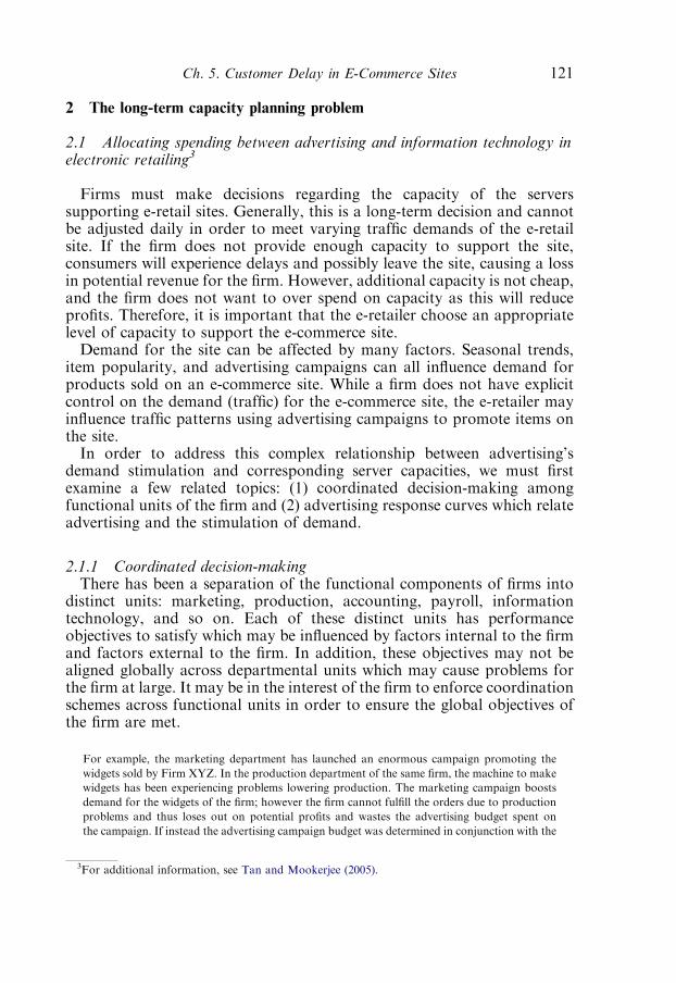
2 The long-term capacity planning problem
2.1 Allocating spending between advertising and information technology inelectronic retailing3
Firms must make decisions regarding the capacity of the serverssupporting e-retail sites. Generally, this is a long-term decision and cannotbe adjusted daily in order to meet varying traffic demands of the e-retailsite. If the firm does not provide enough capacity to support the site,consumers will experience delays and possibly leave the site, causing a lossin potential revenue for the firm. However, additional capacity is not cheap,and the firm does not want to over spend on capacity as this will reduceprofits. Therefore, it is important that the e-retailer choose an appropriatelevel of capacity to support the e-commerce site.Demand for the site can be affected by many factors. Seasonal trends,
item popularity, and advertising campaigns can all influence demand forproducts sold on an e-commerce site. While a firm does not have explicitcontrol on the demand (traffic) for the e-commerce site, the e-retailer mayinfluence traffic patterns using advertising campaigns to promote items onthe site.In order to address this complex relationship between advertising’s
demand stimulation and corresponding server capacities, we must firstexamine a few related topics: (1) coordinated decision-making amongfunctional units of the firm and (2) advertising response curves which relateadvertising and the stimulation of demand.
2.1.1 Coordinated decision-makingThere has been a separation of the functional components of firms into
distinct units: marketing, production, accounting, payroll, informationtechnology, and so on. Each of these distinct units has performanceobjectives to satisfy which may be influenced by factors internal to the firmand factors external to the firm. In addition, these objectives may not bealigned globally across departmental units which may cause problems forthe firm at large. It may be in the interest of the firm to enforce coordinationschemes across functional units in order to ensure the global objectives ofthe firm are met.
For example, the marketing department has launched an enormous campaign promoting the
widgets sold by Firm XYZ. In the production department of the same firm, the machine to make
widgets has been experiencing problems lowering production. The marketing campaign boosts
demand for the widgets of the firm; however the firm cannot fulfill the orders due to production
problems and thus loses out on potential profits and wastes the advertising budget spent on
the campaign. If instead the advertising campaign budget was determined in conjunction with the
3For additional information, see Tan and Mookerjee (2005).
Ch. 5. Customer Delay in E-Commerce Sites 121
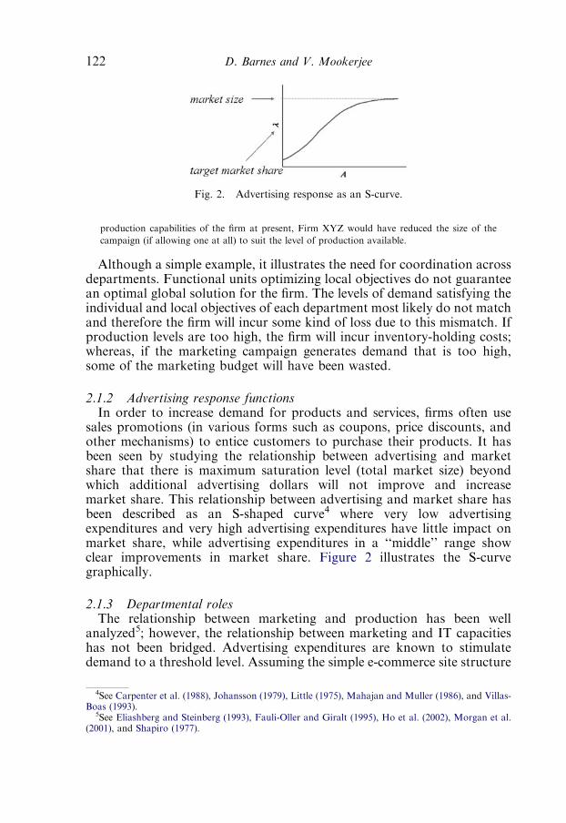
production capabilities of the firm at present, Firm XYZ would have reduced the size of the
campaign (if allowing one at all) to suit the level of production available.
Although a simple example, it illustrates the need for coordination acrossdepartments. Functional units optimizing local objectives do not guaranteean optimal global solution for the firm. The levels of demand satisfying theindividual and local objectives of each department most likely do not matchand therefore the firm will incur some kind of loss due to this mismatch. Ifproduction levels are too high, the firm will incur inventory-holding costs;whereas, if the marketing campaign generates demand that is too high,some of the marketing budget will have been wasted.
2.1.2 Advertising response functionsIn order to increase demand for products and services, firms often use
sales promotions (in various forms such as coupons, price discounts, andother mechanisms) to entice customers to purchase their products. It hasbeen seen by studying the relationship between advertising and marketshare that there is maximum saturation level (total market size) beyondwhich additional advertising dollars will not improve and increasemarket share. This relationship between advertising and market share hasbeen described as an S-shaped curve4 where very low advertisingexpenditures and very high advertising expenditures have little impact onmarket share, while advertising expenditures in a ‘‘middle’’ range showclear improvements in market share. Figure 2 illustrates the S-curvegraphically.
2.1.3 Departmental rolesThe relationship between marketing and production has been well
analyzed5; however, the relationship between marketing and IT capacitieshas not been bridged. Advertising expenditures are known to stimulatedemand to a threshold level. Assuming the simple e-commerce site structure
Fig. 2. Advertising response as an S-curve.
4See Carpenter et al. (1988), Johansson (1979), Little (1975), Mahajan and Muller (1986), and Villas-Boas (1993).
5See Eliashberg and Steinberg (1993), Fauli-Oller and Giralt (1995), Ho et al. (2002), Morgan et al.(2001), and Shapiro (1977).
D. Barnes and V. Mookerjee122
in Fig. 1 the advertising-IT problem is presented. Similar to the productionproblem discussed regarding firm XYZ and the widgets, in an e-commercesetting flooding an e-retailer’s site with requests can actually causeexorbitant wait times and possibly denial of service. In fact, in most firmsIT departments are demand takers, meaning that based on the advertisingbudget allocated for advertising campaigns, IT resources must providesupport for the demand stimulated at the e-retailer’s site. It may be in thebest interest of the firm to evaluate the costs of allowing IT to function as ademand taker such as overspending on capacity. If coordination betweenmarketing and IT can be achieved, the e-retailer may be better off.Marketing department. The marketing department launches advertisingcampaigns in an attempt to increase demand. With no advertising theexisting demand is l0(l0W0). By spending on ad campaigns, demand can beincreased following the S-curve presented in Fig. 2. The specific functionalform which relates the demand level (l) and advertising spending is
A ¼ �a lnl�1 � l�11l�10 � l�11
(1)
where A is the advertising spending, a the advertising cost parameter thatmeasures advertising effectiveness, l0 the initial demand level, and lN thetotal market size.
IT department. The IT department is responsible for processing customerrequests during a session. m represents the capacity of the IT resource (thecatalog server). The larger the value of m the faster the processing ofcustomer session requests.When modeling the loss of customer mathematically, there are many
influencing variables such as the ratio of arrival rate to processing time, theservice rate, and the maximum number of sessions where the services rateand maximum number of sessions both represent site capacity parameters.If the site is experiencing response problems due to maximum number ofsessions then the site would most likely be experiencing a denial of serviceattack, which is not the focus of this discussion. If the maximum number ofsessions is infinite then the number of sessions is not a constraint and theresponse time/service rate(m) can be the object of focus.
2.1.4 Site performance assumptionsIn order to define the site performance characteristics, several assump-
tions regarding demand, processing time, customer impatience, andcustomer time budgets are put in place. As described earlier, customersarrive according to a Poisson distribution. In addition, we focus on thecapacity needs of the Catalog server not the Transaction server asillustrated in Fig. 1.
Ch. 5. Customer Delay in E-Commerce Sites 123
Generic processing time. Each session requires a mean processing time 1/mand a generic distribution (this means that no specific probabilitydistribution has been assumed). The processing time for a session is thetotal time required to process all requests generated during a given session.Due to differing processing time per request there can be a variable numberof requests in a session; therefore, allowing the total processing timedistribution for a session to be generic provides robustness.
Customer impatience. Although customers remain impatient, the server doesnot immediately account for customers who have left due to impatience.Therefore, the loss of impatient customers does not relieve congestion onthe server.
Customer time budgets exponentially distributed. Characterizing the timebudgets as exponential takes advantage of the aforementioned propertythat the time incurred thus far does not impact the likelihood of the timebudget expiring during a discrete future time interval.In general, this scenario can be described as a M/G/1/K/PS queue
(Exponential, General, One-Server, K-Connections, Processor-Sharing). Mrefers to the memory-less nature of the arrivals to the queue expressed bythe exponential inter-arrival times characterized in Poisson countingprocesses. The remaining elements are expressed as follows: (G) processingtimes are generic, (1) one-server, (K) possible sessions at a time and (PS) ashared processor.
2.1.5 Centralized planner caseIn a centralized setting, the firm is a profit maximizer, and hopes to
balance the revenues generated from the site, the cost of additionalcapacity, and the cost of advertising. The e-retailer’s profit function can bewritten as:
p � Sðl;mÞ � ðg0 þ g1mÞ � AðlÞ (2)
where S(l,m) is the net revenue based on the value of arriving customers lessthe lost customers (h(l�L)). m is a variable in the revenue function as theprocessing capacity will determine how many customers are processed andalso those that are lost. (g0 þ g1m) is the IT cost and A(l) is the advertisingcost based on the S-curve response function discussed earlier in (Eq. (1)).Neither the IT department or the marketing department have accessto all of this information; therefore, a centralized planner must solve thisproblem collecting the IT capacity costs from the IT department, theadvertising costs from the marketing department, and compute the revenuefunction.By evaluating the profits, demand levels, and processing capacity with
respect to the change of advertising and capacity costs using the partial
D. Barnes and V. Mookerjee124

derivatives, we find the following:
@F
@ao0 and
@F
@g1o0 (3)
where F ¼ p�, l�, m� the optimal profit, demand level, and processingcapacity respectively.From the first partial derivative ((@F/@a)o0) we can see that as
advertising becomes more costly IT capacity should be reduced, and fromthe second (@F/@g1)o0 that as IT capacity becomes more costly advertisingshould be reduced. With an increase in the cost of advertising or ITcapacity, it is intuitive that both the optimal demand level and the ITcapacity should decrease. For example, if the advertising cost parameter(a) is held constant while the IT capacity cost l1 is increased, the e-retailershould decrease capacity. In addition, this has a negative impact on thenumber of sessions that can be processed and completed. Therefore, thelevel of advertising should also be adjusted downward, even though the costof advertising has been held constant. This example highlights theimportance of coordinating the marketing and IT functions. In adecentralized setting, marketing chooses a demand level, based purely onthe advertising cost parameter, a. However, it is clear from the aboveargument that IT capacity cost should be considered by marketing to arriveat the optimal level of advertising.
2.1.6 Uncoordinated caseIf IT is set up as a demand taker then the marketing department will
choose a demand level l and derive value (hl�A) without considering thecapacity issues the IT department may face based on this trafficperturbation. There is inherent asymmetry in this setting: marketingchooses demand locally, whereas IT reacts to this demand with an optimalchoice for the capacity. This case is uncoordinated as there is nocooperation across the IT and Marketing departments. Based on thegiven demand level, the IT department chooses a capacity level m andderives value (hL(l, m)�g0�g1m) balancing the value of lost customers withthe cost of capacity. Marketing overspends on advertising to attractmore demand than what is optimal, causing IT to incur too much cost forincreasing capacity. In this case, over-advertisement will result in the lossof profit. In fact, profit in decentralized case becomes worse as cost of ITcapacity increases. This shows additional support for the need to coordinatethe marketing and IT decisions. When an appropriate coordinationscheme is imposed, the optimal demand level and IT capacity can beachieved.
Ch. 5. Customer Delay in E-Commerce Sites 125
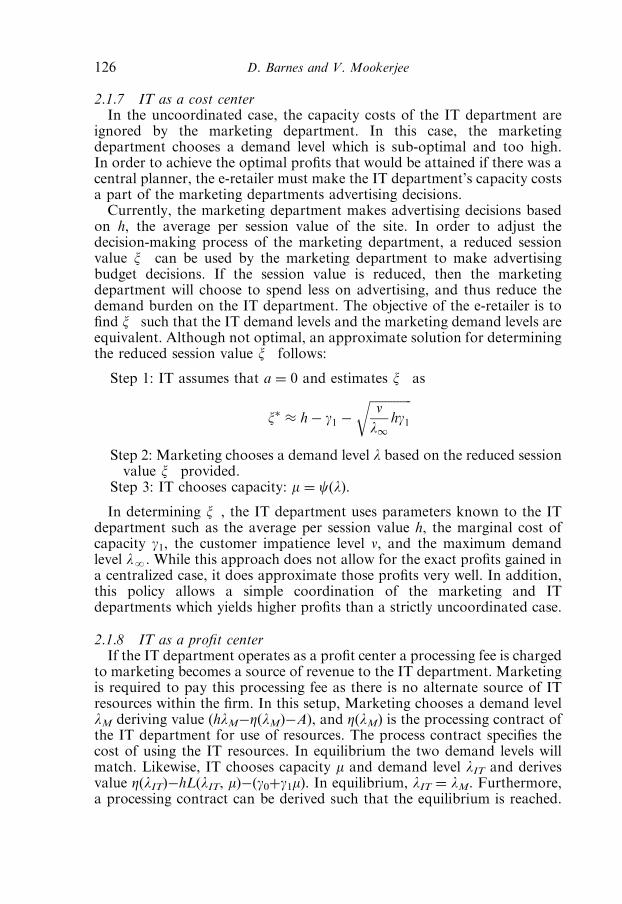
2.1.7 IT as a cost centerIn the uncoordinated case, the capacity costs of the IT department are
ignored by the marketing department. In this case, the marketingdepartment chooses a demand level which is sub-optimal and too high.In order to achieve the optimal profits that would be attained if there was acentral planner, the e-retailer must make the IT department’s capacity costsa part of the marketing departments advertising decisions.Currently, the marketing department makes advertising decisions based
on h, the average per session value of the site. In order to adjust thedecision-making process of the marketing department, a reduced sessionvalue x� can be used by the marketing department to make advertisingbudget decisions. If the session value is reduced, then the marketingdepartment will choose to spend less on advertising, and thus reduce thedemand burden on the IT department. The objective of the e-retailer is tofind x� such that the IT demand levels and the marketing demand levels areequivalent. Although not optimal, an approximate solution for determiningthe reduced session value x� follows:
Step 1: IT assumes that a ¼ 0 and estimates x� as
x h� g1 �ffiffiffiffiffiffiffiffiffiffiffiffiffiffinl1
hg1
r
Step 2: Marketing chooses a demand level l based on the reduced sessionvalue x� provided.
Step 3: IT chooses capacity: m ¼ c(l).
In determining x�, the IT department uses parameters known to the ITdepartment such as the average per session value h, the marginal cost ofcapacity g1, the customer impatience level n, and the maximum demandlevel lN. While this approach does not allow for the exact profits gained ina centralized case, it does approximate those profits very well. In addition,this policy allows a simple coordination of the marketing and ITdepartments which yields higher profits than a strictly uncoordinated case.
2.1.8 IT as a profit centerIf the IT department operates as a profit center a processing fee is charged
to marketing becomes a source of revenue to the IT department. Marketingis required to pay this processing fee as there is no alternate source of ITresources within the firm. In this setup, Marketing chooses a demand levellM deriving value (hlM�Z(lM)�A), and Z(lM) is the processing contract ofthe IT department for use of resources. The process contract specifies thecost of using the IT resources. In equilibrium the two demand levels willmatch. Likewise, IT chooses capacity m and demand level lIT and derivesvalue Z(lIT)�hL(lIT, m)�(g0þg1m). In equilibrium, lIT ¼ lM. Furthermore,a processing contract can be derived such that the equilibrium is reached.
D. Barnes and V. Mookerjee126
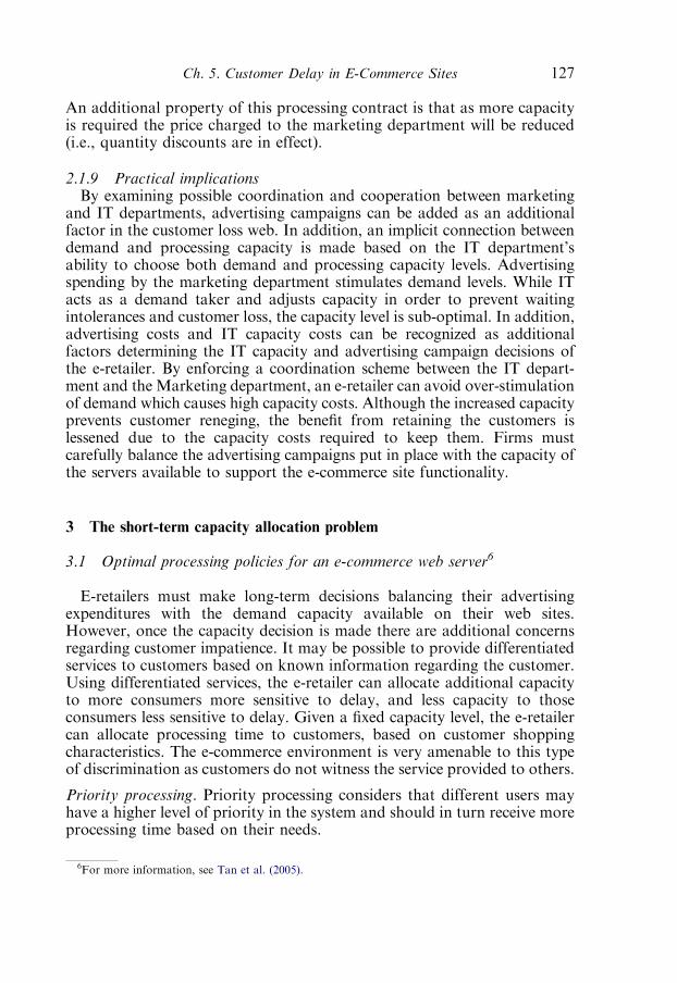
An additional property of this processing contract is that as more capacityis required the price charged to the marketing department will be reduced(i.e., quantity discounts are in effect).
2.1.9 Practical implicationsBy examining possible coordination and cooperation between marketing
and IT departments, advertising campaigns can be added as an additionalfactor in the customer loss web. In addition, an implicit connection betweendemand and processing capacity is made based on the IT department’sability to choose both demand and processing capacity levels. Advertisingspending by the marketing department stimulates demand levels. While ITacts as a demand taker and adjusts capacity in order to prevent waitingintolerances and customer loss, the capacity level is sub-optimal. In addition,advertising costs and IT capacity costs can be recognized as additionalfactors determining the IT capacity and advertising campaign decisions ofthe e-retailer. By enforcing a coordination scheme between the IT depart-ment and the Marketing department, an e-retailer can avoid over-stimulationof demand which causes high capacity costs. Although the increased capacityprevents customer reneging, the benefit from retaining the customers islessened due to the capacity costs required to keep them. Firms mustcarefully balance the advertising campaigns put in place with the capacity ofthe servers available to support the e-commerce site functionality.
3 The short-term capacity allocation problem
3.1 Optimal processing policies for an e-commerce web server6
E-retailers must make long-term decisions balancing their advertisingexpenditures with the demand capacity available on their web sites.However, once the capacity decision is made there are additional concernsregarding customer impatience. It may be possible to provide differentiatedservices to customers based on known information regarding the customer.Using differentiated services, the e-retailer can allocate additional capacityto more consumers more sensitive to delay, and less capacity to thoseconsumers less sensitive to delay. Given a fixed capacity level, the e-retailercan allocate processing time to customers, based on customer shoppingcharacteristics. The e-commerce environment is very amenable to this typeof discrimination as customers do not witness the service provided to others.
Priority processing. Priority processing considers that different users mayhave a higher level of priority in the system and should in turn receive moreprocessing time based on their needs.
6For more information, see Tan et al. (2005).
Ch. 5. Customer Delay in E-Commerce Sites 127

That is, based on a user’s priority class, the users will be allocateddifferent quantum. For example, the higher the priority, the longer theprocessing time allocated to the user. Implementation of priority processingsystems can vary. For example, a modified Round-Robin processing systemcan be used where the time slot is modified by the priority class level. Thistype of priority processing requires that the priority level of jobs are knownex ante.While priority processing schemes have been put in place for resources
shared by a firm’s internal members, in the e-commerce context, where theusers are external to the firm’s boundaries, it is more difficult to implementeffective priority processing schemes. The firm’s objectives are tied tounknown consumer characteristics such as the consumer’s willingness tobuy, the amount the consumer will spend, the probability that the consumerwill renege (leave the site before purchase), and other factors notdetermined by the firm. The firm wishes to keep the consumers who willspend the most while balancing the processing required for those users.Therefore, establishing a priority-processing scheme in this e-commercecontext will be more difficult for the firm than the traditional internalscenario.As aforementioned, the objective of the firm is to implement a priority-
processing scheme which will allocate capacity to optimize some firm goals.In a super market we see express lanes designed to reduce delay forcustomers with fewer items. This is an example of a priority scheme.Consumers with fewer items are more likely to leave without purchasingtheir items; therefore, providing them priority check out allows the firm toretain these consumers. Likewise, e-commerce firms need to implementsimilar priority processing systems based on the characteristics ofconsumers. Instead of using a server which allocates equal quantum basedon Round-Robin approach, firms should implement a server which usesconsumer characteristics to assign priority classes and time slots.
3.2 Environmental assumptions
In order to define the environment, several assumptions are maderegarding the expected purchase value of consumers, the time to process anorder and impatience of consumers, the rate at which consumers arrive atthe site, and finally that a Round-Robin processing scheme is in place.
Static purchase value. Specifically, the purchase value of a given consumer isstatic throughout the course of shopping. This means that the currentbehavior of the consumer does not drive the assigned purchase value. Usinghistorical data, the firm can compute averages of previous visits to the site,or assign a pre-determined value such as the market-average for first timevisitors. The predicted purchase value of a customer (denoted by h) followsa distribution f(h). In fact, the e-retailer can determine both the processing
D. Barnes and V. Mookerjee128

time and the delay tolerance (customer impatience) based on the staticpurchase value assigned to them initially. The only information needed bythe e-retailer is the static purchase value of the customer.
Value-dependent delay tolerance and processing time. Customer impatiencemay lead to the customer leaving the system if their tolerance for waiting(delay tolerance) is exceeded. Again referring to the express lane example,customers with a low purchase value (generally fewer items) have a lowerdelay tolerance and therefore should be given priority while customers witha high purchase value (generally more items) have a higher delay toleranceand can be made to wait. Specifically, customers with a static purchasevalue h will be willing to wait a random time that is exponentiallydistributed with a mean w(h).7
Exponential processing time. Characterizing the processing time (t(h))as exponential implies that the lifetime of the consumer in the system isexponentially distributed. This implies that the probability of a consumerleaving the system in a discrete future time interval, given they have been inthe system 1 millisecond or an infinite time, is just as likely; therefore, theprocessing time incurred does not impact the likelihood of the processingcompleting during a discrete future time interval.
Round-Robin processing. Round-Robin processing is commonly used inprominent e-commerce server software and takes advantage of the idle timebetween user requests. As mentioned earlier, this type of processing makesbetter use of processing power by dividing the processing time intoprocessing units allocated to each user.
3.3 Priority processing scheme
By using the predicted purchase value (h) of a consumer to determine thepriority class k, we can assign processing time g(h)kQ to each priority class(g(h)kZ0), where g(h)k is a priority scheme assigning weights adjusting afixed quantum Q. The e-retailer is concerned with the loss incurred due tointolerable delays on the e-commerce site. The loss function density (l(h))defined as the number of customers lost per unit time per unit value forcustomers with value h is
lðhÞ ¼tðhÞðgðhÞ þ 1Þ
tðhÞðgðhÞ þ 1Þ þ wðhÞgðhÞlf ðhÞ (4)
t(h) is the processing time per customer. w(h) is the mean delay tolerance.g(h) is the priority assigned. l is the arrival rate of consumers to the catalogserver. f(h) is the value distribution of h. We now want to examine how the
7For further justification of this assumption, see Ancker and Gafarian (1962).
Ch. 5. Customer Delay in E-Commerce Sites 129

priority scheme (g(h)k) impacts this loss. We will examine two possiblepriority schemes: a Profit-focused policy and a Quality of Service (QoS)focused policy.
3.4 Profit-focused policy
In this problem the e-retailer determines the priority weights bymaximizing profits. Priority weights will be assigned such that thee-retailer’s profits will be the highest.The e-retailer’s problem is to choose capacity and processing weight to
maximize expected profit per unit time. The total expected revenue (per unittime) is
S ¼
Zh2H
hðlf ðhÞ � lðhÞÞdh (5)
where (lf(h)�l(h)) are the Net Customers with value h. In addition, theserviceable set (the set of customers worth retaining) is
HS ¼ h :h
tðhÞ� c; h 2 H
� �(6)
This expression denotes that the ratio of the static value to the processingtime should be greater than a threshold value c.8 Therefore, only customerswho exceed this threshold value will be allotted processing time. Thisdemonstrates that the e-retailer is interested in balancing the predictedpurchase value (value gained) with the amount of time needed to gain thatvalue (processing time).The priority weights need to be determined. In this case, continuous
priority weights are determined based on the delay tolerance, predictedpurchase value, and processing time of a given user. The expression for thepriority scheme is as follows:
gðhÞ ¼
1
1þwðhÞ=tðhÞ1þ
1
ch
tðhÞ� 1
� �1þ
wðhÞ
tðhÞ
� �� �1=2
� 1
!; h 2HS
0; heHS
8>><>>:
(7)
Therefore, given any h value the firm first decides whether or not theindividual will be serviced based on the determined serviceable set HS andthen assigns a priority weight using the above expression to determine thecustomer’s capacity allocation. By examining the partial derivatives of the
8For details regarding the derivation of these expressions see Tan et al. (2005).
D. Barnes and V. Mookerjee130

priority weights with respect to the rate of revenue realization (h/t(h)) andpriority to processing ratio (w(h)/t(h)) we find
i:@g hð Þ
@ h=t hð Þ 40
ii:@g hð Þ
@ w hð Þ=t hð Þ o0
(8)
These results can be interpreted as follows: (i.) customers with a higher rateof revenue realization receive more processing and (ii.) customers with ahigher value of priority to patience can tolerate more delay and hencereceive less processing time.Profits may not be the only variable of interest to an e-retailer. While
profits are certainly important to all firms, some may wish to focus oncustomer satisfaction and reducing customer loss due to poor servicequality rather than on a policy that treats the customer as a dollar sign.
3.5 Quality of service (QoS) focused policy
In this policy, the e-retailer assigns priority weights such that lostcustomers are minimized. With QoS as the performance objective, thee-retailers’ problem becomes
minL �
Zh2H
lðhÞdh (9)
when (Eq. (4)) defines l(h). This means that the objective of the e-retailer isto minimize the loss of customers.The optimal processing allocation can be obtained as
gðhÞ ¼1
1þwðhÞ=tðhÞ 1þ tctðhÞ � 1� �
1þ wðhÞtðhÞ
� �� �1=2� 1
� �; tðhÞotc
0; tðhÞ � tc
8><>: (10)
It is obvious from the nature of the above equation that customers whorequire more processing (with higher values of 1/t(h)) will be assigned lesspriority.More patient buyers (with higher w(h)/t(h) ratio) also receive lessprocessing time. The value threshold hc is given by t(hc) ¼ tc, and can befound by substituting the above into (Eq. (1)). Assuming t(h) increases withthe value h, customers with value above the value threshold hc will notreceive any processing capacity.Because of the nature of the policies, the profit-focused policy will
outperform the QoS-focused policy when profit is the performance variableand vice versa when only a single-period performance variable is considered.
Ch. 5. Customer Delay in E-Commerce Sites 131
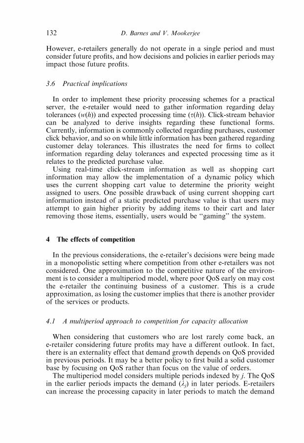
However, e-retailers generally do not operate in a single period and mustconsider future profits, and how decisions and policies in earlier periods mayimpact those future profits.
3.6 Practical implications
In order to implement these priority processing schemes for a practicalserver, the e-retailer would need to gather information regarding delaytolerances (w(h)) and expected processing time (t(h)). Click-stream behaviorcan be analyzed to derive insights regarding these functional forms.Currently, information is commonly collected regarding purchases, customerclick behavior, and so on while little information has been gathered regardingcustomer delay tolerances. This illustrates the need for firms to collectinformation regarding delay tolerances and expected processing time as itrelates to the predicted purchase value.Using real-time click-stream information as well as shopping cart
information may allow the implementation of a dynamic policy whichuses the current shopping cart value to determine the priority weightassigned to users. One possible drawback of using current shopping cartinformation instead of a static predicted purchase value is that users mayattempt to gain higher priority by adding items to their cart and laterremoving those items, essentially, users would be ‘‘gaming’’ the system.
4 The effects of competition
In the previous considerations, the e-retailer’s decisions were being madein a monopolistic setting where competition from other e-retailers was notconsidered. One approximation to the competitive nature of the environ-ment is to consider a multiperiod model, where poor QoS early on may costthe e-retailer the continuing business of a customer. This is a crudeapproximation, as losing the customer implies that there is another providerof the services or products.
4.1 A multiperiod approach to competition for capacity allocation
When considering that customers who are lost rarely come back, ane-retailer considering future profits may have a different outlook. In fact,there is an externality effect that demand growth depends on QoS providedin previous periods. It may be a better policy to first build a solid customerbase by focusing on QoS rather than focus on the value of orders.The multiperiod model considers multiple periods indexed by j. The QoS
in the earlier periods impacts the demand (lj) in later periods. E-retailerscan increase the processing capacity in later periods to match the demand
D. Barnes and V. Mookerjee132
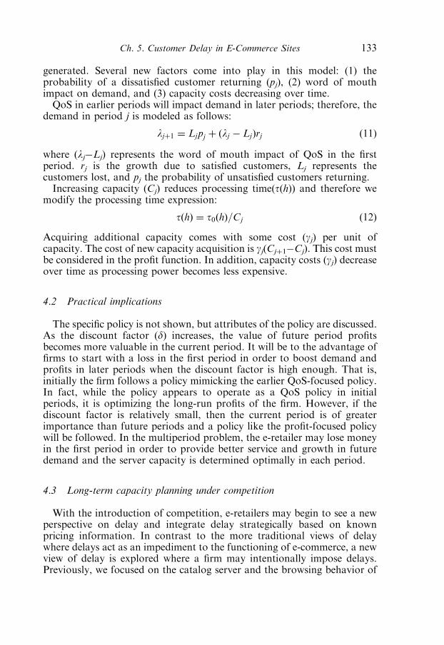
generated. Several new factors come into play in this model: (1) theprobability of a dissatisfied customer returning (pj), (2) word of mouthimpact on demand, and (3) capacity costs decreasing over time.QoS in earlier periods will impact demand in later periods; therefore, the
demand in period j is modeled as follows:
ljþ1 ¼ Ljpj þ ðlj � LjÞrj (11)
where (lj�Lj) represents the word of mouth impact of QoS in the firstperiod. rj is the growth due to satisfied customers, Lj represents thecustomers lost, and pj the probability of unsatisfied customers returning.Increasing capacity (Cj) reduces processing time(t(h)) and therefore we
modify the processing time expression:
tðhÞ ¼ t0ðhÞ=Cj (12)
Acquiring additional capacity comes with some cost (gj) per unit ofcapacity. The cost of new capacity acquisition is gj(Cjþ1�Cj). This cost mustbe considered in the profit function. In addition, capacity costs (gj) decreaseover time as processing power becomes less expensive.
4.2 Practical implications
The specific policy is not shown, but attributes of the policy are discussed.As the discount factor (d) increases, the value of future period profitsbecomes more valuable in the current period. It will be to the advantage offirms to start with a loss in the first period in order to boost demand andprofits in later periods when the discount factor is high enough. That is,initially the firm follows a policy mimicking the earlier QoS-focused policy.In fact, while the policy appears to operate as a QoS policy in initialperiods, it is optimizing the long-run profits of the firm. However, if thediscount factor is relatively small, then the current period is of greaterimportance than future periods and a policy like the profit-focused policywill be followed. In the multiperiod problem, the e-retailer may lose moneyin the first period in order to provide better service and growth in futuredemand and the server capacity is determined optimally in each period.
4.3 Long-term capacity planning under competition
With the introduction of competition, e-retailers may begin to see a newperspective on delay and integrate delay strategically based on knownpricing information. In contrast to the more traditional views of delaywhere delays act as an impediment to the functioning of e-commerce, a newview of delay is explored where a firm may intentionally impose delays.Previously, we focused on the catalog server and the browsing behavior of
Ch. 5. Customer Delay in E-Commerce Sites 133

the consumer, in this case the browsing behavior is also considered;however users are seeking specific information regarding product pricesthat can be found at multiple e-retailers.Waiting at a web site for a consumer may not have a negative impact on a
user’s evaluation of the site if the waiting is well-managed. Consumers tendnot to get as frustrated if the waiting occurs at expected positions likebefore the web text appears on the screen and not in the middle ofinteraction. Thus, a ‘‘well managed’’ delay is one that is not in the middle ofa sensitive transaction, like the transmission of personal informationincluding financial information. Thus it is conceivable that an e-retailerdesign its site in a way to engage the customer and make the experienceenjoyable enough so that the probability of a purchase increases despitetaking a longer time. This Strategic Engagement Model in attempts tocapture the strategic motives of e-retailers that are associated with buildingdelay into their interaction with potential customers.There are two e-firms, firm 1 and firm 2 selling an identical product. The
firms have identical engagement costs c(ti), where dc(ti)/dtW0. Engagementcosts increase with the delay or engagement time (ti) that is built into thebrowsing process by firm j (where j ¼ 1 or 2) at its web site.9 Thus an e-firmneeds to incur higher costs (computing and personnel resources, operatingcosts, etc.) in order to keep customers engaged for a longer time.The consumer side of the market comprises of homogenous agents, who
have unit demand for the product and always buy from the firm with thelower price if they discover that price. A representative consumer does notbrowse indefinitely in order to discover the price, but has a search timebudget t that is known to both firms, and may be defined as the maximumtime spent for the purpose of price discovery. The consumer randomlychooses one of the web sites to begin the search for the lower price. If thetime budget is expended without discovering the price offered by the secondsite, a purchase is made from the first site. No purchase is made if neitherprice is discovered. If both prices are discovered, then the product ispurchased from the lower priced firm. The prices (p1Wp2) charged arecommon knowledge to the firms. The firms interact strategically, settingdelay times in a simultaneous game. We calculate the firms’ best responsedelay functions and solve for the Nash equilibrium in delays.For the lower priced firm 2, it is good strategy to display its price upfront
without any delay or engagement time. If it is the first firm to be visited bythe consumer, all firm 2 needs to do is to display its price in the shortesttime. A longer period of price discovery will merely augment its costswithout increasing its expected profit. If firm 2 is the second to be visitedthen too its optimal strategy is to provide the smallest possible pricediscovery time as any longer than the minimum time would increase the
9This is also the time taken by a potential customer for price discovery at a firm.
D. Barnes and V. Mookerjee134

chances of the consumer’s time budget (t) being exceeded. If e (eW0) is thesmallest time period that a firm can use to display its price, then the optimalengagement time for firm 2 (t2) is
t2 ¼ � (13)
The higher priced firm 1 knows that the only way it can affect a sale is bynot allowing the other (lower priced) firm to display its price to theconsumer. Thus its optimal strategy is to set its engagement time an e abovet�t2, the remainder of the time budget after subtracting firm 2’s choice ofdelay.10
t1 ¼ t� t2 þ � (14)
Mapping out the best response functions for firms 1 and 2 in Fig. 3 we getthe pure strategy Nash equilibrium (NE) given by (t, e) which are the NEstrategies for firms 1 and 2 respectively. Thus the cheaper vendor makes itsprice discovery almost instantaneous while the more expensive providerattempts to engage the potential customer and exhaust the search timebudget.
Fig. 3. Pure strategy Nash equilibrium of the engagement model.
10Notice that the higher priced firm can never win the consumer if it is visited second. The higherpriced firm makes a sale only if it is visited first and sets its delay so that the consumer exhausts the timebudget before discovering the lower priced firm’s price. However, the higher priced firm should not builddelays any higher than e above the ‘‘available’’ time (t�t2) since engagement time is costly.
Ch. 5. Customer Delay in E-Commerce Sites 135
4.4 Practical applications and future adaptations
The basic wisdom from the theoretical result above, namely cheaper firmsaffect quicker price discovery and do not attempt to invest in engaging acustomer is seen in e-commerce interfaces all over the World Wide Web. Ifwe compare car loan web sites with more established loan agencies likeChase Automotive Finance, we find that the former, which typically offerlower APRs and a ‘‘bad credit, no problem’’ attitude has a much quickerprice (in this case the interest rate) discovery than the latter. Organizationslike Chase invest in making the customer go through many ‘‘personalized’’steps (ostensibly for benefiting the customer), but in reality may just beattempting to engage customers long enough in order to induce them tosign them up for a loan. A similar pattern is observed in the onlineprovision of health insurance. Lower premium e-tailers like AffordableHealth Insurance Quotes have a quicker price discovery than larger andmore established insurance firms.Several extensions can be made to the current model. It may be useful to
consider a model where the cost of engagement time includes a technologycost component that reduces with time, for example, the total cost ofengagement could be expressed as: c(t) ¼ a(t)þb(t), where a(t) increaseswith time whereas b(t) (technology cost) decreases with time. This may leadto interior solutions to the game. Another extension is to consider n firms tosee if the basic intuition (high priced firms deliberately delay customers)carries through in the general case. It may also be useful to modelconsumers as being impatient, i.e., they may leave a slow web site with someprobability even if their time budget has not been exhausted. Finally, it willbe interesting to conduct an experiment to see if the model predictscorrectly with human search agents.
5 Conclusions and future research
There are many issues and perspectives related to customer loss caused bydelays in e-commerce settings. In the last section, delay is examined as astrategic tool for an e-retailer; however, this tool can only be enabled in acompetitive environment. An e-retailer’s view of delay may change basedon the competitive context. Therefore the firm’s competitive environmentwhich could be monopolistic or competitive becomes an additionalconsideration for customer loss.In addition, forcing coordination between IT departments and the
Marketing department is in a firm’s best interest. If IT is treated as ademand taker, the Marketing department over spends on advertisingforcing the IT department to make sub-optimal capacity decisions. Whilethese sub-optimal capacity decisions are made in an effort to preventcustomer delay and eventually customer loss, the cost of the capacity is not
D. Barnes and V. Mookerjee136

compensated. Using contracts from the IT department for IT resources, theMarketing department sees IT capacity as a cost and the IT departmentgains revenues from providing resources. This contract enables thedepartments to work in cooperation to set demand levels in an optimalfashion, and aligns the incentives of the departments. Alternatively, the ITdepartment can generate a reduced average session value for the marketingdepartment to consider. This reduced average session value helps accountfor the capacity costs experienced by the IT department and drives thedemand level decisions for each department towards an optimal choice.Capacity adjustments in e-retailer servers are essential to providing
quality service. In fact, quality of service is more important to an e-retailertrying to build a customer base in early periods. By implementing priorityprocessing schemes that focus on maintaining the customer base initially,the e-retailer builds his market share. Later, once the market share isstationary, the e-retailer can maintain his market share using profit-focusedpriority processing schemes.In addition to an e-commerce environment, an online decision support
system environment such as an online help desk may also have queuingeffects as discussed in Sections 2 and 3. Capacity planning and allocationwill be important decisions in this domain as well. We will also investigatethe issue of queuing externalities in the context of decision-orientedsystems. The analysis and design of such systems has been greatly facilitatedby the use Sequential Decision Models (SDM). These models provide apowerful framework to improve system operation. The objective is tooptimize cost or value over a horizon of sequential decisions. In sequentialdecision-making, the decision maker is assumed to possess a set of beliefsabout the state of nature and a set of payoffs about alternatives. Thedecision maker can either make an immediate decision given current beliefsor make a costly observation to revise current beliefs. The next observationor input to acquire depends on the values of previously acquired inputs. Forexample, a physician collects relevant information by asking questions orconducting clinical tests in an order that depends on the specific case. Onceenough information has been acquired, the decision maker selects the bestalternative.Consider an example of an e-business information system where
customers log on to a web site to obtain advice on health related matters.Because of queuing effects, customers may have to wait before and/orduring the consulting session. The operating policy could adjust (increasesor decreases) the quality of the advice offered by the system depending onthe length of the queue. Such a policy may aim to optimize an objectivesuch as the total expected cost incurred, namely, the sum of the expectederror cost (associated with the advice offered by the system) and theexpected waiting cost.The examination of delay experienced in an e-retail environment is of
utmost important in the modern age where much business is transacted
Ch. 5. Customer Delay in E-Commerce Sites 137
online. Just as firms have carefully planned the logistics of their brick andmortar stores, so must they pay special attention to the logistics of their webpresence. Customers who are impatient may leave the e-store with theslightest delay; therefore firms must carefully examine the value that may belost for any given customer type. Understanding the behaviors and value ofthe individual customer will allow the firms to strategically design the webpresence with an appropriate amount of delay.
References
Ancker, C.J., A.V. Gafarian (1962). Queuing with impatient customers who leave at random. Journal of
Industrial Engineering 13, 84–90.
Burman, D. (1981). Insensitivity in queuing systems. Advances in Applied Probability 13, 846–859.
Carpenter, G.S., L.G. Cooper, D.M. Hanssens, D.F. Midgley (1988). Modeling asymmetric
competition. Marketing Science 7, 393–412.
Eliashberg, J., R. Steinberg (1993). Marketing-production joint decision making, in: J. Elizashberg, G.L.
Lilien (eds.), Marketing, DHandbooks in Operations Research and Management Science, Vol. 5.
Elsevier, North Holland.
Fauli-Oller, R., M. Giralt (1995). Competition and cooperation within a multidivisional firm. Journal of
Industrial Economics XLIII, 77–99.
Ho, T.-H., S. Savin, C. Terwiesch (2002). Managing demand and sales dynamics in new product
diffusion under supply constraint. Management Science 48(4), 402–419.
Johansson, J.K. (1979). Advertising and the S-curve: A new approach. Journal of Marketing Research
XVI 346–354.
Little, J.D.C. (1975). BRANDAID: A marketing mix model part 1: Structure. Operations Research 23,
628–655.
Mahajan, V., E. Muller (1986). Advertising pulsing policies for generating awareness for new products.
Marketing Science 5, 86–106.
Morgan, L.O., R.L. Daniels, P. Kouvelis (2001). Marketing/manufacturing tradeoffs in product line
management. IIE Transactions 33 949–962.
O’Donovan, T.M. (1974). Direct solution of M/G/1 processor sharing models. Operations Research 22,
1232–1235.
Ross, S.M. (2000). Introduction to Probability Models. 7th ed. Harcourt Academic Press.
Sakata, M., S. Noguchi, J. Oizumi (1971). An analysis of the M/G/1 queue under round-robin
scheduling. Operations Research 19, 371–385.
Shapiro, B.P. (1977). Can marketing and manufacturing coexist? Harvard Business Review 55, 104–114.
Tan, Y., K. Moionzaeh, V.S. Mookerjee (2005). Optimal processing policies for an e-commerce web
server. Informs Journal on Computing 17(1), 99–110.
Tan, Y., V.S. Mookerjee (2005). Allocating spending between advertising and information technology in
electronic retailing. Management Science 51(8), 1236–1249.
Villas-Boas, J.M. (1993). Predicting advertising pulsing policies in and oligopoly: A model and empirical
test. Marketing Science 12, 88–102.
D. Barnes and V. Mookerjee138

Part II
Computational Approaches
for Business Processes

This page intentionally left blank

Adomavicius & Gupta, Eds., Handbooks in Information Systems, Vol. 3
Copyright r 2009 by Emerald Group Publishing Limited
Chapter 6
An Autonomous Agent for Supply Chain Management
David Pardoe and Peter StoneDepartment of Computer Sciences, The University of Texas at Austin, 1 University Station CO500,
Austin, TX 78712-0233, USA
Abstract
Supply chain management (SCM) involves planning for the procurement ofmaterials, assembly of finished products from these materials, and distribu-tion of products to customers. The Trading Agent Competition Supply ChainManagement (TAC SCM) scenario provides a competitive benchmarkingenvironment for developing and testing agent-based solutions to SCM.Autonomous software agents must perform the above tasks while competingagainst each other as computer manufacturers: each agent must purchasecomponents such as memory and hard drives from suppliers, manage afactory where computers are assembled, and negotiate with customers to sellcomputers. In this chapter, we describe TacTex-06, the winning agent in the2006 TAC SCM competition. TacTex-06 operates by making predictionsabout the future of the economy, such as the prices that will be offered bycomponent suppliers and the level of customer demand, and then planning itsfuture actions in order to maximize profits. A key component of TacTex-06 isthe ability to adapt these predictions based on the observed behavior of otheragents. Although the agent is described in full, particular emphasis is given toagent components that differ from the previous year’s winner, TacTex-05,and the importance of these components is demonstrated through controlledexperiments.
1 Introduction
In today’s industrial world, supply chains are ubiquitous in themanufacturing of many complex products. Traditionally, supply chains havebeen created through the interactions of human representatives of the variouscompanies involved. However, recent advances in autonomous agent
141
technologies have sparked an interest, both in academia and in industry, inautomating the process (Chen et al., 1999; Kumar, 2001; Sadeh et al., 2001).Creating a fully autonomous agent for supply chain management (SCM) isdifficult due to the large number of tasks such an agent must perform. Ingeneral, the agent must procure resources for, manage the assembly of, andnegotiate the sale of a completed product. To perform these tasks intelligently,the agent must be able to plan in the face of uncertainty, schedule the optimaluse of its resources, and adapt to changing market conditions.One barrier to SCM research is that it can be difficult to benchmark
automated strategies in a live business environment, both due to theproprietary nature of the systems and due to the high cost of errors. TheTrading Agent Competition Supply Chain Management (TAC SCM)scenario provides a unique testbed for studying and prototyping SCMagents by providing a competitive environment in which independentlycreated agents can be tested against each other over the course of manysimulations in an open academic setting. A particularly appealing feature ofTAC is that, unlike in many simulation environments, the other agents arereal profit-maximizing agents with incentive to perform well, rather thanstrawman benchmarks.In a TAC SCM game, each agent acts as an independent computer
manufacturer in a simulated economy. The agent must procure componentssuch as CPUs and memory; decide what types of computers to manufacturefrom these components as constrained by its factory resources; bid for salescontracts with customers; and decide which computers to deliver to whomand by when.In this chapter, we describe TacTex-06 , the winner of the 2006 TAC SCM
competition. In particular, we describe the various components that makeup the agent and discuss how they are combined to result in an effectiveSCM agent. Emphasis is given to those components that differ from theprevious year’s winner, TacTex-05, and the importance of these componentsis demonstrated through controlled experiments. The remainder of thechapter is organized as follows. We first summarize the TAC SCM scenario,and then give an overview of the design of TacTex-06 . Next, we describe indetail the individual components: three predictive modules, two decision-making modules that attempt to identify optimal behavior with respect tothe predictions, and two methods of adapting to opponent behavior basedon past games. Finally, we examine the success of the complete agent,through both analysis of competition results and controlled experiments.
2 The TAC SCM scenario
In this section, we provide a summary of the TAC SCM scenario. Fulldetails are available in the official specification document (Collins et al.,2005).
D. Pardoe and P. Stone142

In a TAC SCM game, six agents act as computer manufacturers in asimulated economy that is managed by a game server. The length of a gameis 220 simulated days, with each day lasting 15 s of real time. At thebeginning of each day, agents receive messages from the game server withinformation concerning the state of the game, such as the customer requestsfor quotes (RFQs) for that day, and agents have until the end of the day tosend messages to the server indicating their actions for that day, such asmaking offers to customers. The game can be divided into three parts:(i) component procurement, (ii) computer sales, and (iii) production anddelivery as explained below and illustrated in Fig. 1.
2.1 Component procurement
The computers are made from four components: CPUs, motherboards,memory, and hard drives, each of which come in multiple varieties. Fromthese components, 16 different computer configurations can be made. Eachcomponent has a base price that is used as a reference point by suppliersmaking offers.Agents wanting to purchase components send RFQs to suppliers
indicating the type and quantity of components desired, the date on whichthey should be delivered, and a reserve price stating the maximum amount
Fig. 1. The TAC SCM Scenario (Collins et al., 2005).
Ch. 6. An Autonomous Agent for Supply Chain Management 143

the agent is willing to pay. Agents are limited to sending at most five RFQsper component per supplier per day. Suppliers respond to RFQs the nextday by offering a price for the requested components if the request can besatisfied. Agents may then accept or reject the offers.Suppliers have a limited capacity for producing components, and this
capacity varies throughout the game according to a random walk. Suppliersbase their prices offered in response to RFQs on the fraction of theircapacity that is currently free. When determining prices for RFQs for aparticular component, a supplier simulates scheduling the production of allcomponents currently ordered plus those components requested in theRFQs as late as possible. From the production schedule, the supplier candetermine the remaining free capacity between the current day and anyfuture day. The price offered in response to an RFQ is equal to the baseprice of the component discounted by an amount proportional to thefraction of the supplier’s free capacity before the due date. Agents may sendzero-quantity RFQs to serve as price probes. Due to the nature of thesupplier pricing model, it is possible for prices to be as low whencomponents are requested at the last minute as when they are requested wellin advance. Agents thus face an interesting tradeoff : they may eithercommit to ordering while knowledge of future customer demand is stilllimited (see below), or wait to order and risk being unable to purchaseneeded components.To prevent agents from driving up prices by sending RFQs with no
intention of buying, each supplier keeps track of a reputation rating for eachagent that represents the fraction of offered components that have beenaccepted by the agent. If this reputation falls below a minimum acceptablepurchase ratio (75% for CPU suppliers and 45% for others), then the pricesand availability of components are affected for that agent. Agents musttherefore plan component purchases carefully, sending RFQs only whenthey believe it is likely that they will accept the offers received.
2.2 Computer sales
Customers wishing to buy computers send the agents RFQs consisting ofthe type and quantity of computer desired, the due date, a reserve priceindicating the maximum amount the customer is willing to pay percomputer, and a penalty that must be paid for each day the delivery is late.Agents respond to the RFQs by bidding in a first-price auction: the agentoffering the lowest price on each RFQ wins the order. Agents are unable tosee the prices offered by other agents or even the winning prices, but they doreceive a report each day indicating the highest and lowest price at whicheach type of computer sold on the previous day.Each RFQ is for between 1 and 20 computers, with due dates ranging
from 3 to 12 days in the future, and reserve prices ranging from 75% to
D. Pardoe and P. Stone144

125% of the base price of the requested computer type. (The base price of acomputer is equal to the sum of the base prices of its parts.)The number of RFQs sent by customers each day depends on the level of
customer demand, which fluctuates throughout the game. Demand isbroken into three segments, each containing about one-third of the 16computer types: high, mid, and low range. Each range has its own level ofdemand. The total number of RFQs per day ranges between roughly 80 and320, all of which can be bid upon by all six agents. It is possible for demandlevels to change rapidly, limiting the ability of agents to plan for the futurewith confidence.
2.3 Production and delivery
Each agent manages a factory where computers are assembled. Factoryoperation is constrained by both the components in inventory and assemblycycles. Factories are limited to producing roughly 360 computers per day(depending on their types). Each day an agent must send a productionschedule and a delivery schedule to the server indicating its actions for thenext day. The production schedule specifies how many of each computerwill be assembled by the factory, while the delivery schedule indicates whichcustomer orders will be filled from the completed computers in inventory.Agents are required to pay a small daily storage fee for all components ininventory at the factory. This cost is sufficiently high to discourage agentsfrom holding large inventories of components for long periods.
3 Overview of TacTex-06
Given the detail and complexity of the TAC SCM scenario, creating aneffective agent requires the development of tightly coupled modules forinteracting with suppliers, customers, and the factory. The fact that eachday’s decisions must be made in less than 15 s constrains the set of possibleapproaches.TacTex-06 is a fully implemented agent that operates within the TAC
SCM scenario. We present a high-level overview of the agent in this section,and full details in the sections that follow.
3.1 Agent components
Figure 2 illustrates the basic components of TacTex-06 and theirinteraction. There are five basic tasks a TAC SCM agent must perform:
(1) Sending RFQs to suppliers to request components;(2) Deciding which offers from suppliers to accept;
Ch. 6. An Autonomous Agent for Supply Chain Management 145
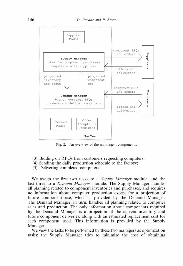
(3) Bidding on RFQs from customers requesting computers;(4) Sending the daily production schedule to the factory;(5) Delivering completed computers.
We assign the first two tasks to a Supply Manager module, and thelast three to a Demand Manager module. The Supply Manager handlesall planning related to component inventories and purchases, and requiresno information about computer production except for a projection offuture component use, which is provided by the Demand Manager.The Demand Manager, in turn, handles all planning related to computersales and production. The only information about components requiredby the Demand Manager is a projection of the current inventory andfuture component deliveries, along with an estimated replacement cost foreach component used. This information is provided by the SupplyManager.We view the tasks to be performed by these two managers as optimization
tasks: the Supply Manager tries to minimize the cost of obtaining
projectedinventoryand costs
Suppliers
Customers
SupplierModel
Demand Managerbid on customer RFQs
produce and deliver computers
OfferAcceptancePredictor
Supply Managerplan for component purchasesnegotiate with suppliers
DemandModel
TacTex
component RFQsand orders
offers anddeliveries
computer RFQsand orders
offers anddeliveries
projectedcomponentuse
Fig. 2. An overview of the main agent components.
D. Pardoe and P. Stone146

the components required by the Demand Manager, whereas the DemandManager seeks to maximize the profits from computer sales subject tothe information provided by the Supply Manager. In order to performthese tasks, the two managers need to be able to make predictions about theresults of their actions and the future of the economy. TacTex-06 usesthree predictive models to assist the managers with these predictions: apredictive Supplier Model, a predictive Demand Model, and an OfferAcceptance Predictor.The Supplier Model keeps track of all information available about each
supplier, such as TacTex-06’s outstanding orders and the prices that havebeen offered in response to RFQs. Using this information, the SupplierModel can assist the Supply Manager by making predictions concerningfuture component availability and prices.The Demand Model tracks the customer demand in each of the three
market segments, and tries to estimate the underlying demand parametersin each segment. With these estimates, it is possible to predict the number ofRFQs that will be received on any future day. The Demand Manager canthen use these predictions to plan for future production.When deciding what bids to make in response to customer RFQs, the
Demand Manager needs to be able to estimate the probability of aparticular bid being accepted (which depends on the bidding behavior of theother agents). This prediction is handled by the Offer Acceptance Predictor.On the basis of past bidding results, the Offer Acceptance Predictorproduces a function for each RFQ that maps bid prices to the predictedprobability of winning the order.The steps taken each day by TacTex-06 as it performs the five tasks
described previously are presented in Table 1.
4 The Demand Manager
The Demand Manager handles all computation related to computer salesand production. This section describes the Demand Manager, along withthe Demand Predictor and the Offer Acceptance Predictor upon which itrelies.
4.1 Demand Model
When planning for future computer production, the Demand Managerneeds to be able to make predictions about future demand in each marketsegment. For example, if more RFQs are expected for high range than lowrange computers, the planned production should reflect this fact. TheDemand Model is responsible for making these predictions.
Ch. 6. An Autonomous Agent for Supply Chain Management 147
To explain its operation, further detail is required about the customerdemand model. The state of each demand segment (high, mid, and lowrange computers) is represented by parameters Qd and td (both of which areinternal to the game server). Qd represents the expected number of RFQs onday d, and td is the trend in demand (increasing or decreasing) on day d.The actual number of RFQs is generated randomly from a Poissondistribution with Qd as its mean. The next day’s demand, Qdþ1, is set toQdtd, and tdþ1 is determined from td according to a random walk.To predict future demand, the Demand Manager estimates the values of
Qd and td for each segment using an approach first used by the agentDeepMaize in 2003 (Kiekintveld et al., 2004). Basically, this is a Bayesianapproach that involves maintaining a probability distribution over (Qd, td)pairs for each segment. The number of RFQs received each day from thesegment represents information that can be used to update this distribution,and the distribution over (Qdþ1, tdþ1) pairs can then be generated based onthe game’s demand model. By repeating this last step, the expected value ofQi can be determined for any future day i and used as the number of RFQspredicted on that day. Full details of the approach are available inKiekintveld et al. (2004).1
Table 1
Overview of the steps taken each day by TacTex-06
Record information received from the server and update prediction modules.
The Supply Manager takes the supplier offers as input and performs the following:
� decide which offers to accept,� update projected future inventory,� update replacement costs.
The Demand Manager takes customer RFQs, current orders, projected inventory,and
replacement costs as input and performs the following:
� predict future customer demand using the Demand Model,� use the Offer Acceptance Predictor to generate acceptance functions for RFQs,� schedule production several days into the future,� extract the current day’s production, delivery, and bids from the schedule,� update projected future component use.
The Supply Manager takes the projected future component use as input andperforms the
following:
� determine the future deliveries needed to maintain a threshold inventory,� use the Supplier Model to predict future component prices,� decide what RFQs need to be sent on the current day.
1The DeepMaize team has released their code for this approach: http://www.eecs.umich.edu/Bckiekint/downloads/DeepMaize_CustomerDemand_Release.tar.gz
D. Pardoe and P. Stone148

4.2 Offer Acceptance Predictor2
To bid on customer RFQs, the Demand Manager needs to be able topredict the orders that will result from the offers it makes. A simple methodof prediction would be to estimate the winning price for each RFQ, andassume that any bid below this price would result in an order. Alternatively,for each RFQ the probability of winning the order could be estimated as afunction of the current bid. This latter approach is the one implemented bythe Offer Acceptance Predictor. For each customer RFQ received, the OfferAcceptance Predictor generates a function mapping the possible bid pricesto the probability of acceptance. (The function can thus be viewed as acumulative distribution function.) This approach involves three compo-nents: a particle filter used to generate initial predictions, an adaptive meansof revising the predictions to account for the impact of an RFQ’s due date,and a learned predictor that predicts how the prices of computers willchange in the future.A visual inspection of each day’s winning prices for each type of
computer in a typical completed game suggests that these prices tend tofollow a normal distribution. To estimate these distributions during a game,the Offer Acceptance Predictor makes use of a separate particle filter[specifically a Sampling Importance Resampling filter (Arulampalam et al.,2002)] for each computer type. A particle filter is a sequential Monte Carlomethod that tracks the changing state of a system by using a set of weightedsamples (called particles) to estimate a posterior density function over thepossible states. The weight of each particle represents its relativeprobability, and particles and weights are revised each time an observation(conditioned on the current state) is received. In this case, each of the 100particles used per filter represents a normal distribution (indicating theprobability that a given price will be the winning price on the computer)with a particular mean and variance. At the beginning of each game,weights are set equally and each particle is assigned a mean and variancedrawn randomly from a distribution that is generated by analyzing the firstday prices from a large data set of past games. (The source of this data setwill be described below.) Each succeeding day, a new set of particles isgenerated from the old. For each new particle to be generated, an oldparticle is selected at random based on weight, and the new particle’sestimate of mean and variance are set to those of the old particle plus smallchanges, drawn randomly from the distribution of day-to-day changes seenin the data set of past games. The new particles are then reweighted, withthe weight of each particle set to the probability of the previous day’s price-related observations occurring according to the distribution represented.These observations consist of the reported highest and lowest winning
2This section presents a significant addition to the previous agent, TacTex-05.
Ch. 6. An Autonomous Agent for Supply Chain Management 149
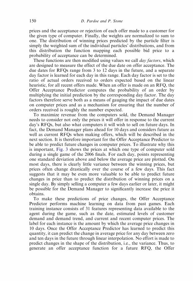
prices and the acceptance or rejection of each offer made to a customer forthe given type of computer. Finally, the weights are normalized to sum toone. The distribution of winning prices predicted by the particle filter issimply the weighted sum of the individual particles’ distributions, and fromthis distribution the function mapping each possible bid price to aprobability of acceptance can be determined.These functions are then modified using values we call day factors, which
are designed to measure the effect of the due date on offer acceptance. Thedue dates for RFQs range from 3 to 12 days in the future, and a separateday factor is learned for each day in this range. Each day factor is set to theratio of actual orders received to orders expected based on the linearheuristic, for all recent offers made. When an offer is made on an RFQ, theOffer Acceptance Predictor computes the probability of an order bymultiplying the initial prediction by the corresponding day factor. The dayfactors therefore serve both as a means of gauging the impact of due dateson computer prices and as a mechanism for ensuring that the number oforders received is roughly the number expected.To maximize revenue from the computers sold, the Demand Manager
needs to consider not only the prices it will offer in response to the currentday’s RFQs, but also what computers it will wish to sell on future days. Infact, the Demand Manager plans ahead for 10 days and considers future aswell as current RFQs when making offers, which will be described in thenext section. It is therefore important for the Offer Acceptance Predictor tobe able to predict future changes in computer prices. To illustrate why thisis important, Fig. 3 shows the prices at which one type of computer soldduring a single game of the 2006 finals. For each day, points representingone standard deviation above and below the average price are plotted. Onmost days, there is clearly little variance between the winning prices, butprices often change drastically over the course of a few days. This factsuggests that it may be even more valuable to be able to predict futurechanges in price than to predict the distribution of winning prices on asingle day. By simply selling a computer a few days earlier or later, it mightbe possible for the Demand Manager to significantly increase the price itobtains.To make these predictions of price changes, the Offer Acceptance
Predictor performs machine learning on data from past games. Eachtraining instance consists of 31 features representing data available to theagent during the game, such as the date, estimated levels of customerdemand and demand trend, and current and recent computer prices. Thelabel for each instance is the amount by which the average price changes in10 days. Once the Offer Acceptance Predictor has learned to predict thisquantity, it can predict the change in average price for any day between zeroand ten days in the future through linear interpolation. No effort is made topredict changes in the shape of the distribution, i.e., the variance. Thus, togenerate an offer acceptance function for a future RFQ, the Offer
D. Pardoe and P. Stone150
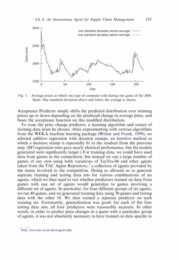
Acceptance Predictor simply shifts the predicted distribution over winningprices up or down depending on the predicted change in average price, andbases the acceptance function on this modified distribution.To train the price change predictor, a learning algorithm and source of
training data must be chosen. After experimenting with various algorithmsfrom the WEKA machine learning package (Witten and Frank, 1999), weselected additive regression with decision stumps, an iterative method inwhich a decision stump is repeatedly fit to the residual from the previousstep. (M5 regression trees gave nearly identical performance, but the modelsgenerated were significantly larger.) For training data, we could have useddata from games in the competition, but instead we ran a large number ofgames of our own using both variations of TacTex-06 and other agentstaken from the TAC Agent Repository,3 a collection of agents provided bythe teams involved in the competition. Doing so allowed us to generateseparate training and testing data sets for various combinations of sixagents, which we then used to test whether predictors trained on data fromgames with one set of agents would generalize to games involving adifferent set of agents. In particular, for four different groups of six agents,we ran 40 games, and we generated training data using 30 games and testingdata with the other 10. We then trained a separate predictor on eachtraining set. Fortunately, generalization was good: for each of the fourtesting data sets, all four predictors were reasonably accurate. In otherwords, in order to predict price changes in a game with a particular groupof agents, it was not absolutely necessary to have trained on data specific to
1200
1800
2400
3000
0 50 100 150 200
Sal
es p
rice
Day
one standard deviation below averageone standard deviation above average
Fig. 3. Average prices at which one type of computer sold during one game of the 2006
finals. One standard deviation above and below the average is shown.
3http://www.sics.se/tac/showagents.php
Ch. 6. An Autonomous Agent for Supply Chain Management 151
those agents. We thus chose to train a single predictor on the entire set ofdata from these games, and use the same predictor throughout thecompetition.4
4.3 Demand Manager
The Demand Manager is responsible for bidding on customer RFQs,producing computers, and delivering them to customers. All three tasks canbe performed using the same production scheduling algorithm. As thesetasks compete for the same resources (components, completed computers,and factory cycles), the Demand Manager begins by planning to satisfyexisting orders, and then uses the remaining resources in planning forRFQs. The latest possible due date for an RFQ received on the current dayis 12 days in the future, meaning the production schedule for the neededcomputers must be sent within the next 10 days. The Demand Managerthus always plans for the next 10 days of production. Each day, theDemand Manager (i) schedules production of existing orders, (ii) schedulesproduction of predicted future orders, and then (iii) extracts the next day’sproduction and delivery schedule from the result. The productionscheduling algorithm, these three steps, and the means of predictingproduction beyond 10 days are described in the following sections.
4.3.1 Production scheduling algorithmThe goal of the production scheduler is to take a set of orders and to
determine the 10-day production schedule that maximizes profit, subject tothe available resources. The resources provided are:
� A fixed number of factory cycles per day;� The components in inventory;� The components projected to be delivered;� Completed computers in inventory.
The profit for each order is equal to its price (if it could be delivered)minus any penalties for late delivery and the replacement costs for thecomponents involved as specified by the Supply Manager.The scheduling algorithm used by the Demand Manager is a greedy
algorithm that attempts to produce each order as late as possible. Ordersare sorted by profit, and the scheduler tries to produce each order usingcycles and components from the latest possible dates. If any part of theorder cannot be produced, the needed computers will be taken from the
4In our post-competition analysis, we found that this was a reasonable decision given the limitednumber of games that would have been available during the competition to use for training. In morerecent work, however, we explore methods of making use of both sources of data (games from thecompetition and games run on our own) and show that improvements in predictor accuracy are possible(Pardoe and Stone, 2007).
D. Pardoe and P. Stone152

existing inventory of completed computers, if possible. The purpose ofscheduling production as late as possible is to preserve resources that mightbe needed by orders with earlier due dates. A record is kept of whatproduction took place on each day and how each order was filled.It should be noted that the scheduling problem at hand lends itself to the
use of linear programming to determine an optimal solution. We initiallyexperimented with this approach, using a linear program similar to onedesigned for a slightly simplified scenario by Benisch et al. (2004a).However, due to the game’s time constraints (15 s allowed per simulatedday), the need to use the scheduler multiple times per day (and in a modifiedfashion for bidding on customer RFQs, as described below), and the factthat the greedy approach is nearly optimal [observed in our ownexperiments and confirmed by Benisch et al. (2006a)], we chose to use thegreedy approach.
4.3.2 Handling existing ordersThe Demand Manager plans for the production of existing orders in two
steps. Before starting, the production resources are initialized using thevalues provided by the Supply Manager. Then the production scheduler isapplied to the set of orders due in one day or less. All orders that can betaken from inventory (hopefully be all of them to avoid penalties) arescheduled for delivery the next day. The production scheduler is nextapplied to the remaining orders. No deliveries are scheduled at this time,because there is no reward for early delivery.
4.3.3 Bidding on RFQs and handling predicted ordersThe goal of the Demand Manager is now to identify the set of bids in
response to customer RFQs that will maximize the expected profit fromusing the remaining production resources for the next 10 days, and toschedule production of the resulting predicted orders. The profit dependsnot only on the RFQs being bid on the current day, but also on RFQs thatwill be received on later days for computers due during the period. If thesefuture RFQs were ignored when selecting the current day’s bids, theDemand Manager might plan to use up all available production resourceson the current RFQs, leaving it unable to bid on future RFQs. One way toaddress this issue would be to restrict the resources available to the agentfor production of the computers being bid on (as in Benisch et al., 2004a).Instead, the Demand Manager generates a predicted set of all RFQs, usingthe levels of customer demand predicted by the Demand Model, that will bereceived for computers due during the period, and chooses bids for theseRFQs at the same time as the actual RFQs from the current day.Once the predicted RFQs are generated, the Offer Acceptance Predictor
is used to generate an acceptance prediction function for every RFQ, bothreal and predicted. The acceptance prediction functions for predicted RFQsare shifted based on the price changes predicted, as described in Section 4.2.
Ch. 6. An Autonomous Agent for Supply Chain Management 153

The Demand Manager then considers the production resources remaining,the set of RFQs, and the set of acceptance prediction functions andsimultaneously generates a set of bids on RFQs and a production schedulethat produces the expected resulting orders, using the following modifica-tion of the greedy scheduler.If we were considering only a single RFQ and had no resource
constraints, the expected profit resulting from a particular bid price wouldbe:
Expected profit ¼ PðorderjpriceÞ ðprice� costÞ (1)
The optimal bid would be the value that maximized this quantity.Computing the expected profit from a set of bids when resource
constraints are considered is much more difficult, however, because theprofit from each RFQ cannot be computed independently. For eachpossible set of orders in which it is not possible to fill all orders, the profitobtained depends on the agent’s production and delivery strategy. For anynontrivial production and delivery strategy, precise calculation of theexpected profit would require separate consideration of a number ofpossible outcomes that is exponential in the number of RFQs. If we wereguaranteed that we would be able to fill all orders, we would not have thisproblem. The expected profit from each RFQ could be computedindependently, and we would have:
Expected profit ¼X
i 2 all RFQs
PðorderijpriceiÞ ðpricei � costiÞ (2)
Our bidding heuristic is based on the assumption that the expectednumber of computers ordered for each RFQ will be the actual numberordered. In other words, we pretend that it is possible to win a part of anorder, so that instead of winning an entire order with probability p, we wina fraction p of an order with probability 1. This assumption greatlysimplifies the consideration of filling orders, since we now have only one setof orders to consider, while leaving the formulation of expected profitunchanged. As long as it is possible to fill the partial orders, (2) will hold,where the probability term now refers to the fraction of the order won. Itwould appear that this approach could lead to unfilled orders when theagent wins more orders than expected, but in practice, this is not generally aproblem. Most of the RFQs being bid on are the predicted RFQs that willbe received on future days, and so the agent can modify its future biddingbehavior to correct for an unexpectedly high number of orders resultingfrom the current day’s RFQs. TacTex-06 indeed tends to have very few lateor missed deliveries using this bidding strategy.By using this notion of partial orders, we can transform the problem of
bid selection into the problem of finding the most profitable set of partialorders that can be filled with the resources available, and we can solve this
D. Pardoe and P. Stone154
problem using the greedy production scheduler. All bids are initially set tobe just above the reserve price, which means we begin with no orders. Thescheduler then chooses an RFQ and an amount by which its bid will belowered, resulting in an increased partial order for that RFQ. The schedulersimulates filling this increase by scheduling its production as describedpreviously. This process is repeated until no more production is possible orno bid can be reduced without reducing the expected profit.Because we are working with resource constraints, the goal of the greedy
production scheduler at each step is to obtain the largest possible increase inprofit using the fewest possible production resources. At each step, thescheduler considers each RFQ and determines the bid reduction that willproduce the largest increase in profit per additional computer. Thescheduler then selects the RFQ for which this value is the largest. In manycases, however, the most limited resource is production cycles, and notcomponents. In such cases, the increase in profit per cycle used is a bettermeasure of the desirability of a partial order than the increase in profit peradditional computer, so we divide the latter quantity by the number ofcycles required to produce the type of computer requested by the RFQ anduse the resulting values to choose which RFQ should be considered next.We consider cycles to be the limiting factor whenever the previous day’sproduction used more than 90% of the available cycles.The range of possible bid prices is discretized for the sake of efficiency.
Even with fairly fine granularity, this bidding heuristic produces a set ofbids in significantly less time than the 15 s allowed per simulated game day.The complete bidding heuristic is summarized in Table 2.
4.3.4 Completing production and deliveryAfter applying the production scheduler to the current orders and RFQs,
the Demand Manager is left with a 10-day production schedule, a record ofhow each order was filled, and a set of bids for the actual and predictedRFQs. The bids on actual RFQs can be sent directly to customers in theircurrent form, and computers scheduled for delivery can be shipped. TheDemand Manager then considers modifications to the production scheduleto send to the factory for the next day. If there are no cycles remaining onthe first day of the 10-day production schedule, the first day can be sentunchanged to the factory. Otherwise, the Delivery Manager shiftsproduction from future days into the first day so as to utilize all cycles, ifpossible.
4.3.5 Production beyond 10 daysThe components purchased by the Supply Manager depend on the
component use projected by the Demand Manager. If we want to allowthe possibility of ordering components more than 10 days in advance, theDemand Manager must be able to project its component use beyond the10-day period for which it plans production. One possibility we considered
Ch. 6. An Autonomous Agent for Supply Chain Management 155

was to extend this period and predict RFQs farther into the future. Anotherwas to predict future computer and component prices by estimating ouropponents’ inventories and predicting their future behavior. Neithermethod provided accurate predictions of the future, and both resulted inlarge swings in projected component use from one day to the next. TheDemand Manager thus uses a simple and conservative prediction of futurecomponent use.The Demand Manager attempts to predict its component use for the
period between 11 and 40 days in the future. Before 11 days, the componentsused in the 10-day production schedule are used as the prediction, andsituations in which it is advantageous to order components more than40 days in advance appear to be rare. The Demand Model is used to predictcustomer demand during this period, and the Demand Manager assumesthat it will win, and thus need to produce, some fraction of this demand.This fraction ranges from zero during times of low demand to 1/6 duringtimes of moderate or high demand, although the Demand Manager will notpredict a higher level of component use than is possible given the availablefactory cycles. While this method of projecting component use yieldsreasonable results, improving the prediction is a significant area for futurework.
5 The Supply Manager
The Supply Manager is responsible for purchasing components fromsuppliers based on the projection of future component use provided by theDemand Manager, and for informing the Demand Manager of expectedcomponent deliveries and replacement costs. In order to be effective, the
Table 2
The bidding heuristic
For each RFQ, compute both the probability of winning and the expected profit as a
function of price.
Set the bid for each RFQ to be just above the reserve price.
Repeat until no RFQs are left in the list of RFQs to be considered:
� For each RFQ, find the bid lower than the current bid that produces the largest increase
in profit per additional computer ordered (or per additional cycle required during periods
of high factory utilization).� Choose the RFQ and bid that produce the largest increase.� Try to schedule production of the partial order resulting from lowering the bid. If it
cannot be scheduled, remove the RFQ from the list.� If the production was scheduled, but no further decrease in the bid will lead to an increase
in profit, remove the RFQ from the list.
Return the final bid for each RFQ.
D. Pardoe and P. Stone156

Supply Manager must be able to predict future component availability andprices. The Supplier Model assists in these predictions.
5.1 Supplier Model
The Supplier Model keeps track of all information sent to and receivedfrom suppliers. This information is used to model the state of each supplier,allowing predictions to be made. The Supplier Model performs three maintasks: predicting component prices, tracking reputation, and generatingprobe RFQs to improve its models.
5.1.1 Price predictionTo assist the Supply Manager in choosing which RFQs to send to
suppliers, the Supplier Model predicts the price that a supplier will offer inresponse to an RFQ with a given quantity and due date. The SupplierModel requires an estimate of each supplier’s existing commitments inorder to make this prediction.Recall that the price offered in response to an RFQ requesting delivery on
a given day is determined entirely by the fraction of the supplier’s capacitythat is committed through that day. As a result, the Supplier Model cancompute this fraction from the price offered. If two offers with different duedates are available, the fraction of the supplier’s capacity that is committedin the period between the first and second date can be determined bysubtracting the total capacity committed before the first date from thatcommitted before the second. With enough offers, the Supplier Model canform a reasonable estimate of the fraction of capacity committed by asupplier on any single day.For each supplier and supply line, the Supply Manager maintains an
estimate of free capacity, and updates this estimate daily based on offersreceived. Using this estimate, the Supplier Model is able to makepredictions on the price a supplier will offer for a particular RFQ.
5.1.2 ReputationWhen deciding which RFQs to send, the Supply Manager needs to be
careful to maintain a good reputation with suppliers. Each supplier has aminimum acceptable purchase ratio, and the Supply Manager tries to keepthis ratio above the minimum. The Supplier Model tracks the offersaccepted from each supplier and informs the Supply Manager of thequantity of offered components that can be rejected from each supplierbefore the ratio falls below the minimum.
5.1.3 Price probesThe Supply Manager will often not need to use the full five RFQs allowed
each day per supplier line. In these cases, the remaining RFQs can be used
Ch. 6. An Autonomous Agent for Supply Chain Management 157

as zero-quantity price probes to improve the Supplier Model’s estimate of asupplier’s committed capacity. For each supplier line, the Supplier Modelrecords the last time each future day has been the due date for an offerreceived. Each day, the Supply Manager informs the Supplier Model of thenumber of RFQs available per supplier line to be used as probes. TheSupplier Model chooses the due dates for these RFQs by finding dates thathave been used as due dates least recently.
5.2 Supply Manager
The Supply Manager’s goal is to obtain the components that the DemandManager projects it will use at the lowest possible cost. This process isdivided into two steps: first the Supply Manager decides what componentswill need to be delivered, and then it decides how best to ensure the deliveryof these components. These two steps are described below, along with analternative means of obtaining components.
5.2.1 Deciding what to orderThe Supply Manager seeks to keep the inventory of each component
above a certain threshold. This threshold (determined experimentally) is800, or 400 in the case of CPUs, and decreases linearly to zero between days195 and 215. Each day the Supply Manager determines the deliveries thatwill be needed to maintain the threshold on each day in the future. Startingwith the current component inventory, the Supply Manager moves througheach future day, adding the deliveries from suppliers expected for that day,subtracting the amount projected to be used by the Demand Manager forthat day, and making a note of any new deliveries needed to maintain thethreshold. The result is a list of needed deliveries that we will call intendeddeliveries. When informing the Demand Manager of the expected futurecomponent deliveries, the Supply Manager will add these intendeddeliveries to the actual deliveries expected from previously placedcomponent orders. The idea is that although the Supply Manager has notyet placed the orders guaranteeing these deliveries, it intends to, and iswilling to make a commitment to the Demand Manager to have thesecomponents available.Because prices offered in response to short-term RFQs can be very
unpredictable, the Supply Manager never makes plans to send RFQsrequesting delivery in less than five days. (One exception is discussed later.)As discussed previously, no component use is projected beyond 40 days inthe future, meaning that the intended deliveries fall in the period between 5and 40 days in the future.
D. Pardoe and P. Stone158

5.2.2 Deciding how to orderOnce the Supply Manager has determined the intended deliveries, it must
decide how to ensure their delivery at the lowest possible cost. We simplifythis task by requiring that for each component and day, that day’s intendeddelivery will be supplied by a single order with that day as the due date.Thus, the only decisions left for the Supply Manager are when to send theRFQ and which supplier to send it to. For each individual intendeddelivery, the Supply Manager predicts whether sending the RFQimmediately will result in a lower offered price than waiting for somefuture day, and sends the RFQ if this is the case.To make this prediction correctly, the Supply Manager would need to
know the prices that would be offered by a supplier on any future day.Although this information is clearly not available, the Supplier Model doeshave the ability to predict the prices that would be offered by a supplier forany RFQ sent on the current day. To enable the Supply Manager to extendthese predictions into the future, we make the simplifying assumption thatthe price pattern predicted on the current day will remain the same on allfuture days. In other words, if an RFQ sent on the current day due in i dayswould result in a certain price, then sending an RFQ on any future day ddue on day dþi would result in the same price. This assumption is notentirely unrealistic due to the fact that agents tend to order components acertain number of days in advance, and this number generally changesslowly. Essentially, we are saying, ‘‘Given the current ordering pattern ofother agents, prices are lowest when RFQs are sent x days in advance of thedue date, so plan to send all RFQs x days in advance.’’The resulting procedure followed by the Supply Manager is as follows.
For each intended delivery, the Supplier Model is asked to predict the pricesthat would result from sending RFQs today with various due datesrequesting the needed quantity. A price is predicted for each due datebetween 5 and 40 days in the future. (Each price is then modified slightlyaccording to a heuristic that will be presented in the next section.) If thereare two suppliers, the lower price is used. If the intended delivery is neededin i days, and the price for ordering i days in advance is lower than that ofany smaller number of days, the Supply Manager will send the RFQ. Anyspare RFQs will be offered to the Supplier Model to use as probes.The final step is to predict the replacement cost of each component. The
Supply Manager assumes that any need for additional components thatresults from the decisions of the Demand Manager will be felt on the firstday on which components are currently needed, i.e., the day with the firstintended delivery. Therefore, for each component’s replacement cost, theSupply Manager uses the lowest price found when considering the firstintended delivery of that component, even if no RFQ was sent.For each RFQ, a reserve price somewhat higher than the expected offer
price is used. Because the Supply Manager believes that the RFQs it sends
Ch. 6. An Autonomous Agent for Supply Chain Management 159

are the ones that will result in the lowest possible prices, all offers areaccepted. If the reserve price cannot be met, the Supplier Model’spredictions will be updated accordingly and the Supply Manager will tryagain the next day.
5.2.3 Waiting to order in certain cases5
When prices are lower for long-term orders than short-term orders, theSupply Manager faces an interesting tradeoff. Waiting to order an intendeddelivery in the short term is expected to increase costs, but by waiting theagent might gain a clearer picture of its true component needs. Forexample, if customer demand suddenly drops, the agent may be better off ifit has waited to order and can avoid unnecessary purchases, even if pricesare somewhat higher for those components which the agent does purchase.Using the ordering strategy of the previous section, however, the SupplyManager would always choose to place long-term orders no matter howsmall the expected increase in cost would be if it waited.A number of experiments using the previous version of the agent,
TacTex-05, suggest that agent performance would improve if the SupplyManager were to postpone ordering in such situations (Pardoe and Stone,2006). One possible way of ensuring this behavior would be to modify thecurrent strategy so that instead of sending a request as soon as the predictedprice is at its lowest point, the request is only sent when it is believed to beunlikely that a reasonably close price can still be obtained. In TacTex-06,the Supply Manager implements an approximation of this strategy using astraightforward heuristic: predictions of offer prices are increased by anamount proportional to the distance of the requested due date. Inparticular, the predicted price for a requested due date d days away,5rdr40, is multiplied by 1þxd, where xd ¼ 0.1�(d�5)/35. Predicted pricesare thus increased between 0% and 10%, values chosen throughexperimentation. As a result, the Supply Manager will wait to order whenlong-term prices are only slightly lower than short-term prices.
5.2.4 2-Day RFQsAs mentioned previously, the prices offered in response to RFQs
requesting near-immediate delivery are very unpredictable. If the SupplyManager were to wait until the last minute to send RFQs in hopes of lowprices, it might frequently end up paying more than expected or be unableto buy the components at all. To allow for the possibility of getting lowpriced short-term orders without risk, the Supply Manager sends RFQs duein 2 days, the minimum possible, for small quantities in addition to what isrequired by the intended deliveries. If the prices offered are lower than thoseexpected from the normal RFQs, the offers will be accepted.
5This section presents a significant addition to the previous agent, TacTex-05.
D. Pardoe and P. Stone160
The size of each 2-day RFQ depends on the need for components, thereputation with the supplier, and the success of past 2-day RFQs. Becausethe Supply Manager may reject many of the offers resulting from 2-dayRFQs, it is possible for the agent’s reputation with a supplier to fall belowthe acceptable purchase ratio. The Supplier Model determines themaximum amount from each supplier that can be rejected before thishappens, and the quantity requested is kept below this amount.The Supply Manager decides whether to accept an offer resulting from a
2-day RFQ by comparing the price to the replacement cost and the prices inoffers resulting from normal RFQs for that component. If the offer price islower than any of these other prices, the offer is accepted. If the quantity inanother, more expensive offer is smaller than the quantity of the 2-dayRFQ, then that offer may safely be rejected.The 2-day RFQs enable the agent to be opportunistic in taking advantage
of short-term bargains on components without being dependent on theavailability of such bargains.
6 Adaptation over a series of games
The predictions made by the predictive modules as described above arebased only on observations from the current game. Another source ofinformation that could be useful in making predictions is the events of pastgames, made available in log files kept by the game server. During the finalrounds of the TAC SCM competition, agents are divided into brackets ofsix and play a number of games (16 on the final day of competition) againstthe same set of opponents. When facing the same opponents repeatedly, itmakes sense to consider adapting predictions in response to completedgames. TacTex-06 makes use of information from these games in itsdecisions during two phases of the game: buying components at thebeginning of the game (impacting mainly the behavior described in Section5.2), and selling computers at the end of the game (impacting the behaviorin Section 4.2). In both cases, only past games within a bracket areconsidered, and default strategies are used when no game logs are yetavailable. We chose to focus on these areas for two reasons. Behaviorduring these two phases varies significantly from one agent to another,possibly due to the fact that these phases are difficult to reason about ingeneral and may thus be handled using special-case heuristic strategies bymany agents. At the same time, each agent’s behavior remains somewhatconsistent from game to game (e.g. many agents order the samecomponents at the beginning of each game). This fact is critical to thesuccess of an adaptive strategy—the limited number of games played meansthat it must be possible to learn an effective response from only a few pastgames.
Ch. 6. An Autonomous Agent for Supply Chain Management 161
6.1 Initial component orders
At the beginning of each game, many agents place relatively largecomponent orders (when compared to the rest of the game) to ensure thatthey will be able to produce computers during the early part of the game.Prices for some components may also be lower on the first day than theywill be afterwards, depending on the due date requested. Determining theoptimal initial orders to place is difficult, because no information is madeavailable on the first day of the game, and prices depend heavily on theorders of other agents.TacTex-06 addresses this issue by analyzing component costs from past
games and deciding what components need to be requested on the first twodays in order to ensure a sufficient supply of components early in the gameand to take advantage of low prices. The process is very similar to the onedescribed in Section 5.2, except that predictions of prices offered bysuppliers are based on past games. First, the components needed areidentified, then the decision of which components should be requested ismade, and finally the RFQs are generated.The Supply Manager begins by deciding what components will be
needed. On the first day, when no demand information is available(customers begin sending RFQs on the second day), the Supply Managerassumes that it will be producing an equal number of each type ofcomputer, and projects the components needed to sustain full factoryutilization for 80 days. On the second day, the Supply Manager projectsfuture customer demand as before and assumes it will receive orders forsome fraction of RFQs over each of the next 80 days. The projectedcomponent use is converted into a list of intended deliveries as before.(The Supply Manager makes no projections beyond the first 80 days,because we have not observed instances where it would be worthwhile toorder components so far in advance.)Next, the Supply Manager must decide which components should be
requested on the current day (the first or second day of the game). As inSection 5.2.2, the Supply Manager must determine which intendeddeliveries will be cheapest if they are requested immediately. At thebeginning of the game, the Supplier Model will have no information to usein predicting prices, and so information from past games is used. Byanalyzing the log from a past game and modeling the state of each supplier,it is possible to determine the exact price that would have been offered inresponse to any possible RFQ. Predictions for the current game can bemade by averaging the results from all past games. When modeling thestates of suppliers, RFQs and orders from TacTex-06 are omitted toprevent the agent from trying to adapt to its own behavior. If the initialcomponent purchasing strategies of opponents remain the same from gameto game, these average values provide a reasonable means of estimatingprices.
D. Pardoe and P. Stone162

At the beginning of the game, the Supply Manager reads in a table from afile that gives the average price for each component for each pair of requestdate and due date. Using this table, the Supply Manager can determinewhich intended deliveries will cost less if requested on the current day thanon any later day. Intended deliveries due within the first 20 days are alwaysrequested on the first day, however, to avoid the possibility that they will beunavailable later. If opponents request many components on the first day ofthe game but few on the second, the prices offered in response to RFQs senton the second day will be about the same as if the RFQs had been sent onthe first day. Since information about customer demand is available on thesecond day of the game but not on the first, it might be beneficial to waituntil the second day to send RFQs. For this reason, the Supply Managerwill not send a request for an intended delivery if the price expected on thesecond day is less than 3% more than the price expected on the first.Once the Supply Manager has decided which intended deliveries to
request, it must decide how to combine these requests into the availablenumber of RFQs (five, or ten if there are two suppliers). In Section 5.2.2,this problem did not arise, because there were typically few requests perday. On the first two days, it is possible for the number of intendeddeliveries requested to be much larger than the number of RFQs available.Intended deliveries will therefore need to be combined into groups, withdelivery on the earliest group member’s delivery date. The choice ofgrouping can have a large impact on the prices offered. When there is onlyone supplier, the Supply Manager begins by dividing the 80-day period intofive intervals, defined by six interval endpoints, with a roughly equalnumber of intended deliveries in each interval. Each interval represents agroup of intended deliveries that will have delivery requested on the firstday of the interval. One at a time, each endpoint is adjusted to minimize thesum of expected prices plus storage costs for those components deliveredearly. When no more adjustments will reduce the cost, the Supply Managersends the resulting RFQs. When there are two suppliers, 10 intervals areused, and intervals alternate between suppliers.
6.2 Endgame sales
Near the end of each game, some agents tend to run out of inventory andstop bidding on computers, whereas other agents tend to have surpluscomputers, possibly by design, that they attempt to sell up until the lastpossible day. As a result, computer prices on the last few days of the gameare often either very high or very low. When endgame prices will be high, itcan be beneficial to hold on to inventory so as to sell it at a premium duringthe last days. When prices will be low, the agent should deplete its inventoryearlier in the game. TacTex-06 adapts in response to the behavior of its
Ch. 6. An Autonomous Agent for Supply Chain Management 163
competitors in past games by adjusting the predictions of the OfferAcceptance Predictor (Section 4.2) during the last few days of each game.TacTex-06’s endgame strategy is essentially to reserve only as many
computers for the final few days as it expects to be able to sell at high prices.In particular, from day 215 to 217, the Demand Manager will alwaysrespond to a customer RFQ (if it chooses to respond) by offering a priceslightly below the reserve. For RFQs received on these days, the probabilitypredicted by the Offer Acceptance Predictor is set to the fraction ofcomputers that would have sold at the reserve price on that day in pastgames. When the Demand Manager plans for a period of production thatincludes one of these days, these acceptance probabilities will hopefully resultin an appropriate number of computers being saved for these three days.
7 2006 Competition results
Out of 21 teams that participated in the final round of the 2006 TACSCM competition, held over three days at AAMAS 2006, six advanced tothe final day of competition. After 16 games between these agents, TacTex-06 had the highest average score, $5.9 million, followed closely byPhantAgent with $4.1 million, and DeepMaize with $3.6 million.6 BothPhantAgent and DeepMaize were much improved over their 2005counterparts, and would very likely have beaten the previous year’schampion, TacTex-05, if it had competed unchanged. It thus appears thatthe improvements present in TacTex-06 were an important part of itsvictory. Although it is difficult to assign credit for an agent’s performance inthe competition to particular components, we can make some observationsthat support this hypothesis.Figure 4 shows the average, over all 16 games on the final day of the
competition, of the profit earned per game day for the top three agents.Daily profit is computed by determining what computers were delivered tocustomers each day and which components in inventory went into thosecomputers, and then subtracting costs from revenue. TacTex-06 clearly hadthe highest daily profits over the first 70 days of the game, and after thispoint profits were roughly equal for all three agents. The difference inprofits appears to be accounted for by higher revenue per computer. Duringthe first 70 days of each game, TacTex-06 sold about as many computers asPhantAgent and DeepMaize while paying roughly the same costs forcomponents, but TacTex-06 almost always had a much higher average salesprice for each type of computer. After day 70, TacTex-06 still hadsomewhat higher average computer prices, but these were offset by highercomponent costs than the other two agents paid.
6Competition scores are available at http://www.sics.se/tac/scmserver
D. Pardoe and P. Stone164
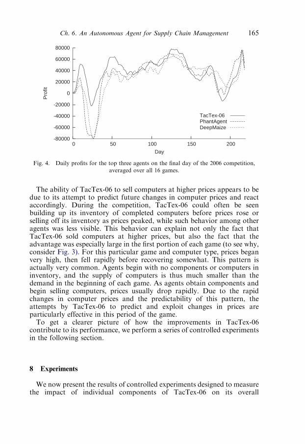
The ability of TacTex-06 to sell computers at higher prices appears to bedue to its attempt to predict future changes in computer prices and reactaccordingly. During the competition, TacTex-06 could often be seenbuilding up its inventory of completed computers before prices rose orselling off its inventory as prices peaked, while such behavior among otheragents was less visible. This behavior can explain not only the fact thatTacTex-06 sold computers at higher prices, but also the fact that theadvantage was especially large in the first portion of each game (to see why,consider Fig. 3). For this particular game and computer type, prices beganvery high, then fell rapidly before recovering somewhat. This pattern isactually very common. Agents begin with no components or computers ininventory, and the supply of computers is thus much smaller than thedemand in the beginning of each game. As agents obtain components andbegin selling computers, prices usually drop rapidly. Due to the rapidchanges in computer prices and the predictability of this pattern, theattempts by TacTex-06 to predict and exploit changes in prices areparticularly effective in this period of the game.To get a clearer picture of how the improvements in TacTex-06
contribute to its performance, we perform a series of controlled experimentsin the following section.
8 Experiments
We now present the results of controlled experiments designed to measurethe impact of individual components of TacTex-06 on its overall
-80000
-60000
-40000
-20000
0
20000
40000
60000
80000
0 50 100 150 200
Pro
fit
Day
TacTex-06PhantAgentDeepMaize
Fig. 4. Daily profits for the top three agents on the final day of the 2006 competition,
averaged over all 16 games.
Ch. 6. An Autonomous Agent for Supply Chain Management 165
performance. In each experiment, two versions of TacTex-06 compete: oneunaltered agent that matches the description provided previously, and oneagent that has been modified in a specific way. Each experiment involves 30games. The other four agents competing—Mertacor, DeepMaize, Minne-TAC, and PhantAgent (all versions from 2005)—are taken from the TACAgent Repository. (Experiments against different combinations of agentsappear to produce qualitatively similar results.)Experimental results are shown in Table 3. Each experiment is labeled
with a number. The columns represent the averages over the 30 games ofthe total score (profit), percent of factory utilization over the game (which isclosely correlated with the number of computers sold), revenue from sellingcomputers to customers, component costs, and the percentage of games inwhich the altered agent outscored the unaltered agent. In every experiment,the difference between the altered and unaltered agent is statisticallysignificant with 99% confidence according to a paired t-test.The first row, experiment 0, is provided to give perspective to the results
of other experiments. In experiment 0, two unaltered agents are used, andall numbers represent the actual results obtained. In all other rows, thenumbers represent the differences between the results of the altered agentand the unaltered agent (from that experiment, not from experiment 0). Ingeneral, the results of the unaltered agents are close to those in experiment0, but there is some variation due to differences between games (e.g.customer demand), and due to the effects of the altered agent on theeconomy.
8.1 Supply price prediction modification
As described in Section 5.2.3, the Supply Manager slightly increases thepredictions of prices that will be offered for components by an amountproportional to the number of days before the requested due date. Thisaddition to TacTex-06 is designed to cause the agent to favor short-termcomponent orders over long-term orders if the difference in price is small.In experiment 1, an agent that does not use this technique is tested.Compared to the unaltered agent, this agent has increased componentpurchases and factory utilization, but the increase in revenue is not enoughto offset the higher costs, and the final score is lower than that of theunaltered agent. It appears that the unaltered agent is able to avoidpurchasing unprofitable components in some cases by waiting longer toplace its orders.
8.2 Offer Acceptance Predictor
We now consider the impact of the improvements to the OfferAcceptance Predictor described in Section 4.2. In experiment 2, the altered
D. Pardoe and P. Stone166
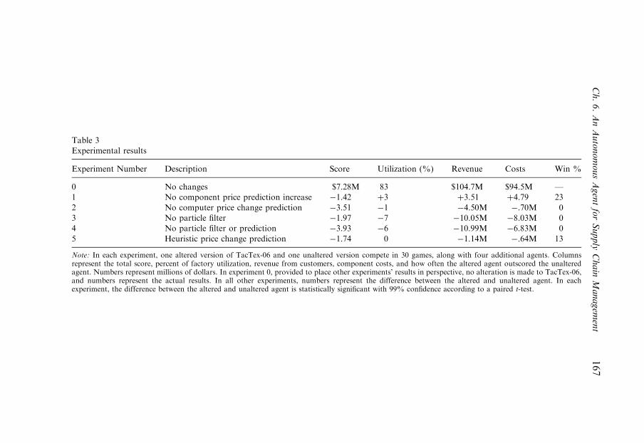
Table 3
Experimental results
Experiment Number Description Score Utilization (%) Revenue Costs Win %
0 No changes $7.28M 83 $104.7M $94.5M —
1 No component price prediction increase �1.42 þ3 þ3.51 þ4.79 23
2 No computer price change prediction �3.51 �1 �4.50M �.70M 0
3 No particle filter �1.97 �7 �10.05M �8.03M 0
4 No particle filter or prediction �3.93 �6 �10.99M �6.83M 0
5 Heuristic price change prediction �1.74 0 �1.14M �.64M 13
Note: In each experiment, one altered version of TacTex-06 and one unaltered version compete in 30 games, along with four additional agents. Columnsrepresent the total score, percent of factory utilization, revenue from customers, component costs, and how often the altered agent outscored the unalteredagent. Numbers represent millions of dollars. In experiment 0, provided to place other experiments’ results in perspective, no alteration is made to TacTex-06,and numbers represent the actual results. In all other experiments, numbers represent the difference between the altered and unaltered agent. In eachexperiment, the difference between the altered and unaltered agent is statistically significant with 99% confidence according to a paired t-test.
Ch.6.AnAutonomousAgentforSupply
Chain
Managem
ent
167
agent always predicts that future computer prices will remain unchanged.Not surprisingly, the result is a large decrease in revenue and score. Thedecrease in score is almost twice as large as the margin of victory forTacTex-06 in the 2006 competition ($1.8 million), adding more weight tothe claim of Section 7 that the prediction of future price changes played alarge role in the winning performance.In experiment 3, the particle filter used to generate predictions of offer
acceptance is replaced with a simpler heuristic that was used in TacTex-05.This heuristic used linear regression over the results of the past five days’offers to generate a linear function used for offer acceptance predictionsand was originally used by the agent Botticelli in 2003 (Benisch et al.,2004a). The experiment shows that the particle filter approach is animprovement over this heuristic. The large drop in factory utilization in thealtered agent is surprising. Experiment 4 shows the result when the changesof experiments 2 and 3 are combined: the agent makes no predictions offuture price changes and uses the linear heuristic instead of the particlefilter. The score is only slightly worse than in experiment 2, suggestingthat the benefits of using the particle filter are more pronounced whenprice changes are predicted. It is possible that the more detailed andprecise predictions of offer acceptance generated from the particle filter arenecessary for the agent to effectively make use of the predictions of futureprice changes.In experiment 5, the learned predictor of price changes is replaced with a
heuristic that performs linear regression on the average computer price overthe last 10 days, and extrapolates the trend seen into the future to predictprice changes. Although the heuristic’s predictions are reasonably accurate,the performance of the altered agent is about midway between that of theunaltered agent and that of the agent from experiment 2 that makes nopredictions at all, demonstrating the value of learning an accuratepredictor.
9 Related work
Outside of TAC SCM, much of the work on agent-based SCM hasfocused on the design of architectures for distributed systems in whichmultiple agents throughout the supply chain must be able to communicateand coordinate (Fox et al., 2000; Sadeh et al., 2001). These systems mayinvolve a static supply chain or allow for the dynamic formation of supplychains through agent negotiation (Chen et al., 1999). Other work hasfocused on general solutions to specific subproblems such as procurementor delivery. TAC SCM appears to be unique in that it represents a concretedomain in which individual agents must manage a complete supply chain ina competitive setting.
D. Pardoe and P. Stone168

A number of agent descriptions for TAC SCM have been publishedpresenting various solutions to the problem. At a high level, many of theseagents are similar in design to TacTex-06: they divide the full problem intoa number of smaller tasks and generally solve these tasks using decision-theoretic approaches based on maximizing utility given estimates of variousvalues and prices. The key differences are the specific methods used to solvethese tasks.The problem of bidding on customer RFQs has been addressed with a
wide variety of solutions. Southampton-SCM (He et al., 2006) takes a fuzzyreasoning approach in which a rule base is developed containing fuzzy rulesthat specify how to bid in various situations. PSUTAC (Sun et al., 2004)takes a similar knowledge-based approach. DeepMaize (Kiekintveld et al.,2004) performs a game-theoretic analysis of the economy to decide whichbids to place. RedAgent (Keller et al., 2004) uses a simulated internalmarket to allocate resources and determine their values, identifying bidprices in the process. The approach described in this chapter, whereprobabilities of offer acceptance are predicted and then used in anoptimization routine, is also used in various forms by several other agents.CMieux (Benisch et al., 2006b) makes predictions using a form of regressiontree that is trained on data from past games, Foreseer (Burke et al., 2006)uses a form of online learning to learn multipliers (similar to the day factorsused in TacTex-06) indicating the impact of various RFQ properties onprices, and Botticelli (Benisch et al., 2004a) uses the heuristic described inSection 8.2.Like TacTex-06, many agents use some form of greedy production
scheduling, but other, more sophisticated approaches have been studied.These include a stochastic programming approach, in which expected profitis maximized through the use of samples generated from a probabilisticmodel of possible customer orders (Benisch et al., 2004b) and an approachtreating the bidding and scheduling problems as a continuous knapsackproblem (Benisch et al., 2006a). In the latter case, an e-optimal solution ispresented which is shown to produce results similar to the greedy approachof TacTex-06, but in significantly less time for large problems.Attention has also been paid to the problem of component procurement,
although much of it has focused on an unintended feature of the game rules(eliminated in 2005) that caused many agents to purchase the majority oftheir components at the very beginning of the game (Kiekintveld et al.,2005). Most agents now employ approaches that involve predictions offuture component needs and prices and are somewhat similar to theapproach described in this chapter. These approaches are often heuristic innature, although there are some exceptions; NaRC (Buffett and Scott,2004) models the procurement problem as a Markov decision process anduses dynamic programming to identify optimal actions.Although several agents make efforts to adapt to changing conditions
during a single game, such as MinneTAC (Ketter et al., 2005) and
Ch. 6. An Autonomous Agent for Supply Chain Management 169

Southampton-SCM (He et al., 2005), to our knowledge methods ofadaptation to a set of opponents over a series of games in TAC SCM havenot been reported on by any other agent. [Such adaptation has been used inthe TAC Travel competition, however, both during a round of competition(Stone et al., 2001), and in response to hundreds of previous games (Stoneet al., 2003).]
10 Conclusions and future work
In this chapter, we described TacTex-06, a SCM agent consisting ofpredictive, optimizing, and adaptive components. We analyzed its winningperformance in the 2006 TAC SCM competition, and found evidence thatthe strategy of exploiting predicted changes in computer prices to increaserevenue played a significant role in this performance. Controlled experi-ments verified the value of a number of improvements made to TacTex-05,the previous winner.A number of areas remain open for future work. There is room for
improvement in many of the predictions, possibly though additional usesof learning. Also, by looking farther ahead when planning offers tocustomers, it may be possible for the agent to better take advantage of thepredicted changes in future prices. In addition, there is the question ofwhat would happen if several agents attempted to utilize such a strategyfor responding to price changes, and what the proper response to thissituation would be.The most important area for improvement, in both TacTex-06 and other
TAC SCM agents, is likely increasing the degree to which agents areadaptive to ensure robust performance regardless of market conditions.While developing TacTex-06, we had the opportunity to carefully tuneagent parameters (such as inventory thresholds) and to test various agentmodifications during several rounds of competition and in our ownexperiments with the available agent binaries. In addition, we were able toimplement learning-based approaches that took advantage of data frompast games. When developing agents for real-world supply chains, suchsources of feedback and experience would be reduced in quantity orunavailable. Although it would still be possible to test agents in simulation,the market conditions encountered upon deployment might differsignificantly from the simulated conditions. Designing agents that canadapt quickly given limited experience is therefore a significant part of ourfuture research agenda.Ultimately, this research drives both towards understanding the
implications and challenges of deploying autonomous agents in SCMscenarios, and towards developing new machine-learning-based completeautonomous agents in dynamic multiagent domains.
D. Pardoe and P. Stone170

Acknowledgments
We would like to thank Jan Ulrich and Mark VanMiddlesworth forcontributing to the development of TacTex, the SICS team for developingthe game server, and all teams that have contributed to the agent repository.This research was supported in part by NSF CAREER award IIS-0237699.
References
Arulampalam, S., S. Maskell, N. Gordon, T. Clapp (2002). A tutorial on particle filters for on-line non-
linear/non-gaussian bayesian tracking. IEEE Transactions on Signal Processing 50(2), 174–188.
Benisch M., A. Greenwald, I. Grypari, R. Lederman, V. Naroditskiy, M. Tschantz (2004a). Botticelli: a
supply chain management agent. in: Third International Joint Conference on Autonomous Agents and
Multiagent Systems (AAMAS), New York, NY, 3, 1174–1181.
Benisch, M., A. Greenwald, V. Naroditskiy, M. Tschantz (2004b). A stochastic programming approach
to scheduling in TAC SCM, in: Fifth ACM Conference on Electronic Commerce, New York, NY,
152–159.
Benisch, M., J. Andrews, N. Sadeh (2006a). Pricing for customers with probabilistic valuations as a
continuous knapsack problem, in: Eighth International Conference on Electronic Commerce,
Fredericton, New Brunswick, Canada.
Benisch, M., A. Sardinha, J. Andrews, N. Sadeh (2006b). Cmieux: adaptive strategies for competitive
supply chain trading, in: Eighth International Conference on Electronic Commerce, Fredericton,
New Brunswick, Canada.
Buffett, S., N. Scott (2004). An algorithm for procurement in supply chain management, in: AAMAS
2004 Workshop on Trading Agent Design and Analysis, New York, NY.
Burke, D.A., K.N. Brown, B. Hnich, A. Tarim (2006). Learning market prices for a real-time supply
chain management trading agent, in: AAMAS 2006 Workshop on Trading Agent Design and Analysis/
Agent Mediated Electronic Commerce, Hakodate, Japan.
Chen, Y., Y. Peng, T. Finin, Y. Labrou, S. Cost (1999). A negotiation-based multi-agent system for
supply chain management, in: Workshop on Agent-Based Decision Support in Managing the Internet-
Enabled Supply-Chain, at Agents ‘99, Seattle, Washington.
Collins, J., R. Arunachalam, N. Sadeh, J. Eriksson, N. Finne, S. Janson (2005). The supply chain
management game for the 2006 trading agent competition. Technical report. Available at http://
www.sics.se/tac/tac06scmspec_v16.pdf
Fox, M.S., M. Barbuceanu, R. Teigen (2000). Agent-oriented supply-chain management. International
Journal of Flexible Manufacturing Systems 12, 165–188.
He, M., A. Rogers, E. David, N.R. Jennings (2005). Designing and evaluating an adaptive trading agent
for supply chain management applications, in: IJCAI 2005 Workshop on Trading Agent Design and
Analysis, Edinborough, Scotland, UK.
He, M., A. Rogers, X. Luo, N.R. Jennings (2006). Designing a successful trading agent for supply chain
management, in: Fifth International Joint Conference on Autonomous Agents and Multiagent Systems,
Hakodate, Japan, 1159–1166.
Keller, P.W., F.-O. Duguay, D. Precup (2004). RedAgent—winner of TAC SCM 2003. SIGecom
Exchanges: Special Issue on Trading Agent Design and Analysis 4(3), 1–8.
Ketter, W., J. Collins, M. Gini, A. Gupta, P. Schrater (2005). Identifying and forecasting economic
regimes in TAC SCM, in: IJCAI 2005 Workshop on Trading Agent Design and Analysis,
Edinborough, Scotland, UK, 53–60.
Kiekintveld, C., M. Wellman, S. Singh, J. Estelle, Y. Vorobeychik, V. Soni, M. Rudary (2004).
Distributed feedback control for decision making on supply chains, in: Fourteenth International
Conference on Automated Planning and Scheduling, Whistler, British Columbia, Canada.
Ch. 6. An Autonomous Agent for Supply Chain Management 171

Kiekintveld, C., Y. Vorobeychik, M.P. Wellman (2005). An analysis of the 2004 supply chain
management trading agent competition, in: IJCAI 2005 Workshop on Trading Agent Design and
Analysis, Edinborough, Scotland, UK.
Kumar, K. (2001). Technology for supporting supply-chain management. Communications of the ACM
44(6), 58–61.
Pardoe, D., P. Stone (2006). Predictive planning for supply chain management, in: Sixteenth
International Conference on Automated Planning and Scheduling, Cumbria, UK.
Pardoe, D., P. Stone (2007). Adapting price predictions in TAC SCM, in: AAMAS 2007 Workshop on
Agent Mediated Electronic Commerce, Honolulu, HI.
Sadeh, N., D. Hildum, D. Kjenstad, A. Tseng (2001). MASCOT: an agent-based architecture for
dynamic supply chain creation and coordination in the Internet economy. Journal of Production,
Planning and Control 12(3), 211–223.
Stone, P., M.L. Littman, S. Singh, M. Kearns (2001). ATTac-2000: an adaptive autonomous bidding
agent. Journal of Artificial Intelligence Research 15, 189–206.
Stone, P., R.E. Schapire, M.L. Littman, J.A. Csirik, D. McAllester (2003). Decision-theoretic bidding
based on learned density models in simultaneous, interacting auctions. Journal of Artificial
Intelligence Research 19, 209–242.
Sun, S., V. Avasarala, T. Mullen, J. Yen (2004). PSUTAC: a trading agent designed from heuristics to
knowledge, in: AAMAS 2004 Workshop on Trading Agent Design and Analysis, New York, NY.
Witten, I.H., E. Frank (1999). Data Mining: Practical Machine Learning Tools and Techniques with Java
Implementations. Morgan Kaufmann, San Francisco, CA.
D. Pardoe and P. Stone172

Adomavicius & Gupta, Eds., Handbooks in Information Systems, Vol. 3
Copyright r 2009 by Emerald Group Publishing Limited
Chapter 7
IT Advances for Industrial Procurement: AutomatingData Cleansing for Enterprise Spend Aggregation
Moninder Singh and Jayant R. KalagnanamIBM T.J. Watson Research Center, 1101 Kitchawan Road, Yorktown Heights, NY 10598, USA
Abstract
The last few years have seen tremendous changes in IT applications targetedtowards improving the procurement activities of an enterprise. The signifi-cant cost savings generated by such changes have in turn led to an evengreater focus on, and investments in, the development of tools and systemsfor streamlining enterprise procurement. While the earliest changes dealt withthe development of electronic procurement systems, subsequent develop-ments involved an increased shift to strategic procurement functions, andconsequently towards the development of tools such as eRFPS and auctionsas negotiation mechanisms. A recent trend is the move towards outsourcingpart or all of the procurement function, especially for non-core procurementpieces, to emerging intermediaries who then provide the procurementfunction for the enterprise. In this practice, called Business TransformationOutsourcing (BTO), such third-parties can substantially reduce procurementcosts, in part by doing procurement on behalf of several different enterprises.An essential aspect of managing this outsourced procurement function is theability to aggregate and analyze the procurement-spend across one or moreenterprises, and rationalize this process. This too requires a new set of ITtools that are able to manage unstructured data and provide ways toefficiently aggregate and analyze spend information across potentially severalenterprises. Typically, these data cleansing tasks are done manually usingrudimentary data analysis techniques and spreadsheets. However, asignificant amount of research has been conducted over the past couple ofdecades in various fields, such as databases, statistics and artificialintelligence, on the development of various data cleansing techniques, andtheir application to a broad range of applications and domains. This chapterprovides a brief survey of these techniques and applications, and thendiscusses how some of these methods can be adapted to automate the variouscleansing activities needs for spend data aggregation. Moreover, the chapter
173
provides a detailed roadmap to enable the development of such an automatedsystem for spend aggregation to enable spend aggregation, especially acrossmultiple enterprises, to be done in an efficient, repeatable and automatedmanner.
1 Introduction
By streamlining its procurement activities, an enterprise can realizesubstantial cost savings that directly impact the bottom line. Additionally,rapid developments in information technology (IT) have made thisstreamlining process significantly faster and cheaper than was possible justa few years ago. As such, more and more enterprises are recognizing this tobe strategically essential and are devoting considerable effort and resourcesto improving their procurement activities, both in terms of reducing thetotal procurement spend as well as using what is spent more effectively.Towards this end, enterprises have been increasingly using IT tools
targeted primarily at the procurement activities of enterprises. Over the pastfew years, these tools have gradually become more and more sophisticated,both from technological and functional aspects. Initially, the focus wasprimarily on the development of electronic systems to assist daily procure-ment activity at an operational level. These were the early ‘‘procurementsystems’’ that focused largely on managing the business process dealingwith operational buying to streamline it to follow procedures andauthorization, as well as to make the requisitioning and payment byelectronic means. Thereafter, tool development moved to tackle some ofthe strategic functions of procurement, such as strategic sourcing. This ledto an increased interest in the use of tools, such as eRFPs and auctions, asa way of negotiating price and non-price aspects of the requirements andsubsequently led to the use of various auctions’ mechanisms for negotiationusing electronic exchanges and portals.The latest trend, however, is towards outsourcing non-core parts of the
procurement function to emerging intermediaries who then provide theprocurement function, especially for non-directs. An essential aspect ofmanaging this outsourced procurement function (as well as for doingstrategic sourcing done for procurement that is done in-house) is the abilityto analyze the procurement-spend of a company (along various dimensionssuch as suppliers and commodities) and rationalize this process. Owing tothis, one of the most important activities that an enterprise has to undertakeprior to doing strategic sourcing or outsourcing its procurement functions isto develop a single, aggregated view of its procurement-spend across theentire enterprise. Since procurement activities take place normally acrossan enterprise, spanning multiple back-end systems and/or geographic and
M. Singh and J.R. Kalagnanam174
functional areas and often using multiple procurement applications, spendaggregation becomes necessary to understand where the money is beingspent, and on what. Once an aggregated, enterprise view of spend isdeveloped, it can be used by the enterprise for various strategic activitiessuch as consolidating suppliers and negotiating better volume-based prices.Spend aggregation becomes an even more essential activity in cases of
procurement outsourcing. In such cases, a form of business transformationoutsourcing (BTO), a third-party (referred to henceforth as a BTO serviceprovider) takes over the procurement functions of one or more enterprises(referred to henceforth as BTO clients). However, in order to do theprocurement efficiently, the BTO service provider needs to aggregatespend across all these enterprises (i.e. the BTO clients plus the BTO serviceprovider itself) so as to develop a consistent supplier base and a consistentcommodity base resulting in an accurate cross-enterprise view of exactlywhat is being procured and from whom. Using this view, the BTO serviceclient too can do significant strategic sourcing (similar to an enterprisedoing strategic sourcing with its internal spend but on a much larger scale),such as evaluating all suppliers from which a particular commodity isacquired, and negotiating better deals with one or more of them based onthe combined volume of that commodity across all the BTO clients.Procurement outsourcing can lead to significant savings for an enterprise,especially since procurement accounts for a major part of enterprise costs.This is due to several reasons. First, by delegating the procurement function(generally a non-core business activity) to a third party, an enterprise canfocus more on its core business operations, streamline its business processesand reduce the complexity and overhead of its operations (by eliminating anactivity in which it does not have much expertise). Second, procurementoutsourcing allows an enterprise to immediately shrink its cost structure byreducing/eliminating procurement-related resources, including headcountas well as hardware and procurement applications. Third, the cost toacquire goods by an enterprise falls since the BTO service providerpasses on some of the savings it generates via the bigger (volume-based)discounts it is able to get by aggregating spend over all its BTO clients,thereby generating higher commodity volumes, and directing that to fewer,preferred suppliers. Moreover, the magnitude of the savings that can begenerated by the BTO service provider are typically higher than what anenterprise could achieve by doing similar activities (such as volumeaggregation, supplier consolidation, etc.) by keeping its procurementactivities in-house. This can be attributed to three main reasons. First,the BTO service provider normally has significant expertise in procurement,and can utilize specialized and more efficient procurement processes.Second, taking on the procurement of multiple enterprises allows the serviceprovider to take advantages of economies of scale. Third, the volume-baseddiscounts that a service provider can negotiate with its suppliers are muchhigher than what any of the client enterprise’s could get by itself, since the
Ch. 7. IT Advances for Industrial Procurement 175
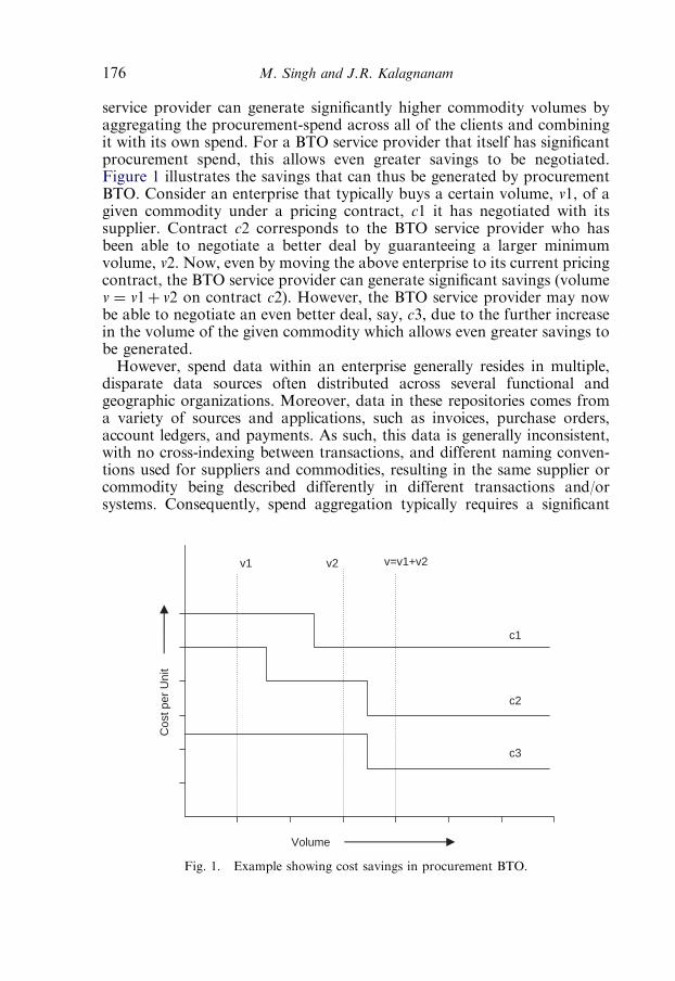
service provider can generate significantly higher commodity volumes byaggregating the procurement-spend across all of the clients and combiningit with its own spend. For a BTO service provider that itself has significantprocurement spend, this allows even greater savings to be negotiated.Figure 1 illustrates the savings that can thus be generated by procurementBTO. Consider an enterprise that typically buys a certain volume, v1, of agiven commodity under a pricing contract, c1 it has negotiated with itssupplier. Contract c2 corresponds to the BTO service provider who hasbeen able to negotiate a better deal by guaranteeing a larger minimumvolume, v2. Now, even by moving the above enterprise to its current pricingcontract, the BTO service provider can generate significant savings (volumev ¼ v1þ v2 on contract c2). However, the BTO service provider may nowbe able to negotiate an even better deal, say, c3, due to the further increasein the volume of the given commodity which allows even greater savings tobe generated.However, spend data within an enterprise generally resides in multiple,
disparate data sources often distributed across several functional andgeographic organizations. Moreover, data in these repositories comes froma variety of sources and applications, such as invoices, purchase orders,account ledgers, and payments. As such, this data is generally inconsistent,with no cross-indexing between transactions, and different naming conven-tions used for suppliers and commodities, resulting in the same supplier orcommodity being described differently in different transactions and/orsystems. Consequently, spend aggregation typically requires a significant
Cos
t per
Uni
t
Volume
v1 v2 v=v1+v2
c1
c3
c2
Fig. 1. Example showing cost savings in procurement BTO.
M. Singh and J.R. Kalagnanam176
amount of effort since the spend data has to be cleansed and rationalized sothat discrepancies between multiple naming conventions get resolved,transactions get mapped to a common spend/commodity taxonomy, etc.Clearly, the level of difficulty, and the effort needed, to do this acrossmultiple enterprises, as required for procurement BTO, gets progressivelyhigher since different supplier bases as well as multiple commoditytaxonomies have to be reconciled and mapped. This has lead to renewedfocus on the development of new tools and methodologies for managingunstructured content inherent in spend data (e.g. commodity descriptions)and cleansing the data to enable spend aggregation, especially across multipleenterprises, to be done in an efficient, repeatable and automated manner.Data cleansing has long been studied in various fields, such as statistics,
databases and machine learning/data mining, resulting in a host of datacleansing techniques that have been applied to a multitude of differentproblems and domains, such as duplicate record detection in databases/data warehouses and linkage of medical records belonging to the sameindividual in different databases. Often, data cleansing has been a laborintensive task requiring substantial human involvement. Automation hasgenerally been addressed only recently and that too in limited cases.Moreover, many of the problems tackled have been of a very specific natureand fairly domain specific. Nevertheless, the underlying techniques behindthe solutions developed have generally been quite similar. Also, some of theproblems addressed (e.g. duplicate detection) have much in common withsome of the cleansing tasks needed for aggregation of enterprise spend.As such, Section 2 provides an overview of various techniques for data
cleansing that have been developed, and applied to various cleansing tasks,over the past few decades. Section 2.1 provides a broad, albeit brief,survey of the main data cleansing techniques and applications, whileSections 2.2–2.4 take three of these techniques that are quite useful fordeveloping automated spend aggregation systems and discusses them indetail as well as highlights their pros and cons for various data cleansingactivities.Subsequently, Section 3 deals with the automation of data cleansing for
spend aggregation, with Section 3.1 detailing the various data cleansingtasks that must be carried out to facilitate effective spend aggregationwithin and across enterprises and Section 3.2 providing a detailed roadmapfor developing an automated system for carrying out those tasks, using datacleansing techniques discussed in Section 2.Finally, we conclude and summarize this discussion in Section 4.
2 Techniques for data cleansing
As discussed previously, data cleansing has been studied in various fieldsand applied to several different problems and domains. Section 2.1 provides
Ch. 7. IT Advances for Industrial Procurement 177
a brief survey some of the data cleansing literature. Section 2.2 then takes acloser look at some of the types of algorithms underlying the commonlyused data cleansing techniques.
2.1 Overview of data cleansing approaches
The data cleansing problem has been studied over several decades undervarious names, such as record linkage (Fellegi and Sunter, 1969; Winkler2002, 2006), duplicate detection (Bitton and Dewitt, 1983; Wang andMadnick, 1989), record matching (Cochinwala et al., 2001), merge/purgeproblem (Hernandez and Stolfo, 1995), etc.1 This task, in general, refers tothe identification of duplicates that may be present in data due to a varietyof reasons, such as errors, different representations or notations, incon-sistencies in the data, etc. While substantial work around this issue has beenconducted in the statistics community with a focus on specific problems,such as record linkage in medical data for identifying medical recordsfor the same person in multiple databases (Jaro, 1995; Newcombe, 1988) orfor matching people across census or taxation records (Alvey andJamerson, 1997; Jaro, 1989), a large body of literature also exists, especiallyin the database literature, on more general, domain-independent datacleaning, especially in the context of data integration and data warehousing(Bright et al., 1994; Dey et al., 2002; Lim and Chiang, 2004; Monge andElkan, 1997).From an algorithmic point of view, the techniques that have been studied
for addressing the data cleansing problem can be broadly categorized intotext similarity methods (Cohen, 2000; Hernandez and Stolfo, 1995; Mongeand Elkan, 1997), unsupervised learning approaches, such as clustering(Cohen and Richman, 2002; Fellegi and Sunter, 1969), and supervisedlearning approaches (Bilenko and Mooney, 2003; Borkar et al., 2000;Winkler, 2002). Winkler (2006) provides an extensive and detailed survey ofdata cleansing approaches that have been developed using methods in oneor more of these categories. A detailed discussion of this subject matter isbeyond the scope of this chapter, and the interested reader is referred toWinkler’s paper cited above, as well as other numerous other survey articles(Cohen et al., 2003; Rahm and Do, 2000). Nevertheless, in the followingsection, we discuss, in some level of detail, a few of the most commonly usedtechniques that are especially suited for the development of automated datacleansing techniques for enterprise spend aggregation.
1We refer to this ‘‘classic’’ data cleansing problem as the ‘‘duplicate detection’’ problem in the rest ofthis chapter.
M. Singh and J.R. Kalagnanam178

2.2 Text similarity methods
Some of the most commonly used methods for data cleansing have theirroots in the information retrieval literature (Baeza-Yates and Ribeiro-Neto,1999). Generally referred to as string or text similarity methods, thesetechniques often measure the ‘‘similarity’’ between different strings (withidentical strings considered to be the most similar) on the basis of somemetric that provides a quantitative measure of the ‘‘distance’’ betweenmultiple strings, the higher the distance between them, the lesser thesimilarity and vice versa.2
One class of such functions are comprised of the so-called edit distancefunctions that measure the distance between strings as a cost-function basedon the minimum number of operations (character insertions, deletions andsubstitutions) needed to transform one string to the other. The Levenshteindistance (LD) (Levenshtein, 1966) is a basic edit distance that assumes aunit cost for each such operation. Several different variations that usedifferent costs for the various operations, as well as extensions of the basicedit distance, have also been proposed (Cohen et al., 2003; Navarro, 2001).Computation of the LD between two strings can be done using dynamicprogramming based on a set of recurrence as described below.Consider the calculation of the LD between two strings, say S and T, with
lengths n and m, respectively. Let S [1 . . . i] (and T [1 . . . j ]) and S [i] (and T [j])represent the substring of the first ‘i’ (and ‘j’) characters and the ith (and jth)character of S (and T ), respectively. Moreover, let LD(S [1 . . . i],T [1 . . . j ]) bethe distance between the substrings comprised of the first ‘i’ characters of Sand the first ‘j’ characters of T. Then, LD(S,T) is given by LD(S [1 . . . n],T[1 . . .m]). It is easy to see that this computation can be done recursively bylooking at the three different ways of transforming S[1 . . . i] to T [1 . . . j].These are (i) converting S [1 . . . i�1] to T [1 . . . j�1] followed by convertingS [i] to T [ j] leading to a cost of LD(S [1 . . . i�1],T [1 . . . j�1] plus the costof replacing S [i] by T [ j] which is either 0 (if same) or 1 (if different),(ii) converting S[1 . . . i�1] to T [1 . . . j] and deleting S [i] leading to a cost ofLD(S [1 . . . i�1],T[1 . . . j])þ 1 and (iii) converting S [1 . . . i] to T [1 . . . j�1] andinserting T [ j ] leading to a cost of LD(S [1 . . . i],T [1 . . . j�1])þ 1. The cost ofconverting S to T then is given by the minimum of these three costs, thus
LD S½1 . . . i�;T ½1 . . . j�ð Þ ¼ min
LDðS½1 . . . i � 1�;T ½1 . . . j � 1�Þ þ Csub
LDðS½1 . . . i � 1�;T ½1 . . . j�Þ þ 1;
LDðS½1 . . . i�;T ½1 . . . j � 1�Þ þ 1
8><>:
where Csub is either 0 or 1 as described in (i) above.
2We use the terms ‘‘similarity’’ and ‘‘distance’’ interchangeably, depending upon the interpretationthat is more commonly used in the literature, with ‘‘higher similarity’’ analogous to ‘‘smaller distance’’and vice versa.
Ch. 7. IT Advances for Industrial Procurement 179

The form of these recurrence relations leads to a dynamic programmingformulation of the LD computation as follows: Let C be a nþ 1 by mþ 1array where C [i,j ] represents LD(S[1 . . . i],T [1 . . . j]). Then, LD(S,T ) ¼LD(S [1 . . . n],T [1 . . .m]) ¼ C[n,m] is calculated by successively computingC[i,j] based on the recurrence relations above as follows:
� Initialization:
C½0; 0� ¼ 0
C½i; 0� ¼ i; 1 � i � n
C½0; j� ¼ j; 1 � j � m
� Calculation: Compute C[i,j] for all nZ i Z1, mZjZ1 using theformula
C½i; j� ¼MinðC½i � 1; j � 1� þ Csub; C½i � 1; j� þ 1;C½i; j � 1�;þ1Þ
where Csub ¼ 1 if S[i] 6¼ T [ j ] and 0 otherwise.
The advantage of using edit distance measures is that they are fairlyrobust to spelling errors and small local differences between strings.However, computation of edit distances, as shown above, can becomputationally expensive, especially when it has to be done repeatedlyfor comparing a large number of strings.Another kind of common distance-based similarity methods work by
breaking up strings into bags of tokens, and computing the distancebetween the strings based on these tokens. Tokens can be words (usingwhite space and punctuation as delimiters), n-grams (consecutiven-character substrings), etc. The simplest way to then measure the similaritybetween the strings is to determine the number of tokens in commonbetween the two strings, the higher the count the greater the similarity.However, since this generally favors longer strings, it is better to usenormalized measures such as Jaccard similarity (Jaccard, 1912), Dicesimilarity (Dice, 1945) or Cosine similarity (Salton and Buckley, 1987).A common way to represent such similarity measures is by considering thestrings, say S and T, as vectors in multi-dimensional vector space andrepresenting them as weight-vectors of the form, S ¼ {s1, . . . , sn} andT ¼ {t1, . . . , tn} where si, ti are the weights assigned to the ith token(in the collection of all n tokens present in the system) for the strings Sand T, respectively. Then, the vector product of the two weight-vectors
Pni¼1siti
measures the number of tokens that are common to
the two strings, and the above-mentioned similarity measures can be
M. Singh and J.R. Kalagnanam180

expressed as follows:
JaccardðS;TÞ ¼
Pni¼1
siti
Pni¼1
s2i þPni¼1
t2i �Pni¼1
siti
(1)
DiceðS;TÞ ¼
2 Pni¼1
siti
Pni¼1
s2i þPni¼1
t2i
(2)
CosineðS;TÞ ¼
Pni¼1
sitiffiffiffiffiffiffiffiffiffiffiPni¼1
s2i
s ffiffiffiffiffiffiffiffiffiffiPni¼1
t2i
s (3)
In this formulation, if the weights si, ti are assigned such that their value is1 if the ith token is present in the corresponding string, and 0 otherwise,then the Jaccard similarity can be seen to be the number of tokens incommon between the two strings, normalized by the total number of uniquetokens in the two strings (union), whereas the Dice similarity can be seen tobe the number of tokens in common between the two strings, normalized bythe average of the number of tokens in the two strings. Cosine similarity isslightly different in that a vector length normalization factor is used wherethe weight of each token depends on the weights of the other tokens in thesame string. Accordingly, in the above formulation (Salton and Buckley,1987), the similarity may be considered to be a vector product of the two
weight vectors, with the individual weights being si=ffiffiffiffiffiffiffiffiffiffiffiffiffiffiffiPn
i¼1s2i
qand
ti=ffiffiffiffiffiffiffiffiffiffiffiffiffiffiffiPn
i¼1t2i
q(instead of si and ti, respectively).
However, these methods do not distinguish between different terms(tokens) in the strings being compared, both in terms of their importance tothe strings containing those tokens or their ability to discriminate suchstrings from other strings not containing those tokens. The TF/IDF (TermFrequency/Inverse Document Frequency) (Salton and Buckley, 1987)approach uses a cosine distance-based similarity measure where each tokenin a string is assigned a weight representing the importance of that term tothat particular string as well as relative to all other strings to which it iscompared. While this approach is commonly used for document retrieval, itcan also be used to measure similarity between different strings in a givenset of strings. In this case, the weight assigned to a token consists of threecomponents: (i) a term frequency component measuring the number of
Ch. 7. IT Advances for Industrial Procurement 181

times the token occurs in the string, (ii) an inverse document frequencycomponent that is inversely proportional to the number of strings in whichthat token occurs and (iii) a normalization component, typically based onthe length of the string vector. While the term frequency componentmeasures the importance of a term to the string in which it is contained, theinverse document frequency component measures its ability to discriminatebetween multiple strings, and the normalization component ensures thelonger strings are not unfairly preferred over smaller strings (since longerstrings, with more tokens, would otherwise have higher likelihood of havingmore tokens in common with the string being compared with, as opposed tosmaller strings). Thus, typically, we define
Term Frequency ðtfÞ ¼ # of times token occurs in the string
Inverse Document Frequency ðidfÞ ¼ logðN=nÞ
where n is the number of strings in which the token occurs in the entirecollection of N strings under consideration.Then, for a string S with a weight-vectors of the form, S ¼ {s1, . . . ,sn}, the
weight of the ith token is specified as
si ¼ tf si idfsi ¼ tfsi logðN=niÞ (4)
Then, the TF-IDF similarity (Salton and Buckley, 1987) between twostrings, say S and T represented as weight-vectors S ¼ {s1, . . . ,sn} and T ¼{t1, . . . ,tn}, respectively, is given by
TF=IDFðS;TÞ ¼
Pni¼1
sitiffiffiffiffiffiffiffiffiffiffiPni¼1
s2i
s ffiffiffiffiffiffiffiffiffiffiPni¼1
t2i
s
¼
Pni¼1
tf si tfti logðN=niÞ 2
ffiffiffiffiffiffiffiffiffiffiffiffiffiffiffiffiffiffiffiffiffiffiffiffiffiffiffiffiffiffiffiffiffiffiffiffiffiffiffiffiffiffiPni¼1
tfsi logðN=niÞ 2s ffiffiffiffiffiffiffiffiffiffiffiffiffiffiffiffiffiffiffiffiffiffiffiffiffiffiffiffiffiffiffiffiffiffiffiffiffiffiffiffiffiffiPn
i¼1
tf ti logðN=niÞ 2s ð5Þ
As can be seen from Eq. (3), this is equivalent to the cosine similaritybetween the two strings (with the token weights defined as in Eq. (4)).Several different variations of this have been studied as well (Salton andBuckley, 1987).
M. Singh and J.R. Kalagnanam182
2.3 Clustering methods
Another class of methods that is especially useful for the cleansingactivities are clustering techniques. The aim of clustering is to partition agiven dataset into a set of groups such that the data items within a groupare ‘‘similar’’ in some way to each other, but ‘‘dissimilar’’ from data itemsbelonging to the other groups. This implies that a good clustering of adataset corresponds to high intra-cluster similarity and low inter-clustersimilarity, and as such depends on how such similarity is measured, as wellas implemented, by a clustering method. Clustering has been used over theyears in various domains and applications such as pattern recognition,image processing, marketing, information retrieval, etc. (Anderberg, 1973;Jain et al., 1999; Jain and Dubes, 1988; Salton, 1991) and a number ofdifferent algorithms have been devised to do such analysis. Here, wedescribe some of the most commonly used methods and discuss theirrelative advantages and disadvantages; the interested reader is referred toJain et al. (1999) for a more general review and discussion of differentclustering techniques.Arguably the simplest and the most widely used clustering technique is
the k-means algorithm (McQueen, 1967). The aim of the k-means clusteringalgorithm is to partition the dataset into a set of k clusters, the value of kbeing assigned a priori. The k-means algorithm starts with an initialpartition of the data into k clusters (this could be done randomly, forexample), and uses a heuristic to search through the space of all possibleclusters by cycling through steps (i) and (ii) as follows: (i) for each cluster,the centroid (mean point) is calculated using the data points currentlyassigned to the cluster and (ii) each data point is then re-assigned to thecluster whose centroid is the least distance from it. This process is continuedtill some convergence criteria is satisfied (e.g. there is no movement of anydata point to a new cluster). Since this is essentially a greedy approach,it generally terminates in a local optimum. The method is very popular dueto the fact that it is easy to implement and is fairly computationallyefficient. However, it assumes that the number of clusters is knownbeforehand and, since the method converges to a local optimal solution,the quality of the clusters found is very sensitive to the initial partition(Selim and Ismail, 1984).Although the k-means algorithm belongs to a wider class of clustering
algorithms called partitioning algorithms (since they construct variouspartitions from the dataset and evaluate them using some criterion),another popular set of clustering techniques are hierarchical clusteringalgorithms which work by creating a hierarchical decomposition (tree) ofthe dataset using some criterion (normally distance based). There aretwo types of hierarchical clustering methods: agglomerative and divisive.While agglomerative methods start with each data item being placed in itsown cluster and then successively merge the clusters until a termination
Ch. 7. IT Advances for Industrial Procurement 183

condition is reached, divisive methods work along the opposite direction,starting with a single cluster consisting of the entire dataset and successivelysplitting them until a stopping criterion is satisfied. The majority ofhierarchical algorithms are agglomerative, differing primarily in thedistance measure used and the method of measuring similarity (distance)between clusters; divisive methods are rarely used and we do not discussthem further.For measuring the distance between clusters, any of an extensive array of
distance measures can be used, including those that are based on similaritymeasures as described previously, as well as various other distance metricsthat have been used for clustering and similar tasks in the literature, such asEuclidean distance, Minkowski metric, Manhattan (or L1) distance, etc.(Cohen et al., 2003; Jain et al., 1999). For measuring the distance betweenclusters, the two most commonly used methods are the single-link andcomplete-link approaches, though other methods have also been used(Jain et al., 1999). In the single-link case, the distance between two clustersis defined as the shortest distance (or maximum similarity) between anymember of one cluster and any member of the other cluster. However, inthe case of maximum linkage the distance between two clusters is defined asthe maximum distance between any member of one cluster and any memberof the other cluster. Of these, the maximum linkage method generally leadsto a higher degree of intra-cluster homogeneity for a given number ofclusters. Once a choice of the distance measure as well as the methodof determining inter-cluster distance is made, agglomerative clusteringproceeds as described above: starting with single-ton clusters, the pair ofclusters (including clusters that have been created by previous merge steps)that have the least distance between them are successively merged till astopping criterion, such as maximum cluster size threshold or maximumintra-cluster distance threshold is reached.Although hierarchical clustering techniques have the advantage (over
k-means) that the number of clusters does not have to be specified a priori,these methods are not as computationally efficient and do not allow anymerge (or split) decision taken earlier on to be reversed later.Yet another class of popular clustering algorithms, called model-based
clustering methods, assumes certain models for the clusters and attempt tooptimize the fit between these models and the data. The most common ofthis class of methods assumes that each of the clusters can be modeled bya Gaussian distribution (Banfield and Raftery, 1993), and thus the entiredata can be modeled by a mixture of Gaussian distributions. The task ofidentifying the clusters then boils down to the estimation of the parametersof the individual Gaussians. The EM algorithm (Dempster et al., 1997) iscommonly used for this parametric estimation. AutoClass (Cheesemanand Stutz, 1996) is another approach that takes a mixture of distributionsapproach in addition to using Bayesian statistics to estimate the mostprobable number of clusters, given the data. While model-based clustering
M. Singh and J.R. Kalagnanam184
allows the use of established statistical techniques, it differs from theapproaches described earlier in that, unlike k-means and hierarchicalclustering approaches that are purely data driven, it requires priorassumptions regarding the component distributions. Additionally, as inthe case of k-means, the number of clusters also has to be specified a priori(except for AutoClass that estimates that).Irrespective of the type of clustering method used, computational
efficiency and scalability become very important issues when clustering isapplied to problems that are characterized by large datasets. This can occurdue to a large number of records in the dataset, high dimensionality of thefeature space, or a large number of underlying clusters into which the dataneeds to be split up. In such situations, the direct applicability of any of thepreviously discussed clustering approaches can become highly computa-tionally intensive, and practically infeasible, especially when the datasetbeing clustered is large due to all these reasons at the same time. Recently,however, new techniques have been developed for performing clusteringefficiently on precisely these kinds of high-dimensional datasets. The mainidea behind such techniques is to significantly reduce the number of timesexact similarity (or distance) measures have to be computed during theclustering process, thereby reducing the computational complexity of theprocess. One such method is the two-stage clustering technique developedby McCallum et al. (2000). In this method, the first stage is a quick anddirty stage in which cheap and approximate distance measures are usedto divide the dataset into a set of overlapping subsets called canopies. Thisis followed by a more rigorous stage where expensive, exact distancecalculations are made only between data items that occur within the samecanopy. By ensuring that the canopies are so constructed such that onlydata items that exist in a common canopy can exist in the same cluster(i.e. clusters cannot span canopies), substantial computational savings areattained by eliminating the exact distance computations between any pairof points that does not belong to the same canopy. Moreover, this allowsany of the standard clustering techniques described previously to be usedduring the second stage; essentially, that clustering approach is usedrepeatedly to cluster smaller datasets corresponding to the canopies, asopposed to performing clustering on the entire dataset as required whenusing a traditional clustering approach directly.
2.4 Classification methods
A third category of methods, as described previously, that can sometimesprove useful for the data cleansing tasks are classification techniques(also commonly referred to as supervised learning methods). Since datacleansing for often involves mapping and manipulation of textual data,fields such as information retrieval and natural language processing offer a
Ch. 7. IT Advances for Industrial Procurement 185
plethora of machine learning techniques that have been found effectivein such domains (e.g. maximum entropy (Nigam et al., 1999), supportvector machines (Joachims, 1998) and Bayesian methods (McCallum andNigam, 1998)).However, classification methods need ‘‘labeled’’ data in order to build/
train classifiers which could then be used for the mapping tasks needed forspend aggregation, such as supplier name normalization and commoditymapping. Such labeled data is, however, not always available. This is instark contrast to the methods described previously, string similaritymethods as well as clustering techniques that have no such requirement,and, hence, are generally used instead of the classification techniques.As such, we do not discuss these approaches in detail but refer the interesteduser to the above-mentioned references. Nevertheless, we do highlight insubsequent sections where classification approaches could be applied,especially in the context of data cleansing for spend aggregation in aprocurement-BTO setting, since cleansed data for a given enterprise couldpotentially provide the labeled data needed for cleansing the data for otherenterprises, especially those in the same industrial sector. Irrespective of theactual approach adopted, two steps are involved in using classificationmethods for data cleansing: (i) learning classification models for predictingone or more attributes of interest (‘‘target’’ attributes) based on the valuesof other attributes and (ii) applying these models to the unmapped data todetermine the appropriate values of the target attributes. Winkler (2006)provides an extensive list of citations to work in the data cleansing literaturebased on the use of supervised learning techniques for data cleansing, andthe interested reader is referred to the same.One particular area, though, in which supervised learning techniques may
be relevant in the context of data cleansing for spend aggregation is in theautomatic parsing and element extraction from free-text address data(Borkar et al., 2000; Califf, 1998). For this specific task, it may be easier toget labeled data by some combination of standard address databases,manual tagging and labeling, as well as the incremental data cleansingactivities that would be performed during procurement BTO as subsequententerprise repositories encounter free-text addresses that have already beencleansed for previous enterprises.
3 Automating data cleansing for spend aggregation
We now turn our attention to the specific task of automating thecleansing and rationalization of spend across an enterprise so that it can beaggregated and analyzed in a meaningful way. In the case of BTO, this datacleansing has to span multiple enterprises, thus leading to a significantlyhigher level of complexity. Spend aggregation has traditionally been donemanually, generally employing spreadsheets and rudimentary, data analysis
M. Singh and J.R. Kalagnanam186
techniques for mapping and normalizing the data prior to aggregation.However, this is an extremely costly and time-intensive process, especiallyfor larger enterprises where the volume and complexity of spend data makesit all the more difficult. Owing to this slow, error-prone and expensivenature of manual cleansing, coupled with the increased focus in this areaalong with the aforementioned rapid developments in various fields such asdatabases, data mining and information retrieval, there has been a steadyshift towards the development of methods and tools that automate at leastsome aspects of this cleansing activity. While some enterprises have turnedto in-house development of automated solutions for cleansing andaggregating their spend data, others use solutions provided by independentsoftware vendors (ISVs) such as Emptoris, VerticalNet and Zycus toaddress their spend aggregation needs. Some of these are pure consultingsolutions in which the ISV takes the spend data from the enterprise,cleanses, aggregates (automatically and/or manually) and analyzes it, andreturns aggregate spend reports back to the enterprise for further action.On the other end are automated spend analysis solutions that are deployedand configured to work directly with the enterprise’s spend data repositoriesand systems to cleanse, aggregate and analyze the data on a continual basis.However, most of these solutions are primarily for aggregating intra-company spend (traditionally referred to as spend analysis); there are fewsolutions that deal explicitly with of inter-company spend aggregationwhich presents many challenges not encountered while aggregating intra-company spend (Singh and Kalagnanam, 2006). In Section 3.1, we discussin detail the various cleansing tasks that must be carried out in order toconvert spend data to a form where effective aggregation is possible, andthe issues that must be addressed in order to enable this cleansing to bedone in an automated manner. We specifically highlight the similarities ofsome of these cleansing tasks with the classic duplicate detection problemand also point out the key points where the two differ. Section 3.2 thenprovides a rough roadmap towards the development of a simple automatedspend-aggregation solution using some of the techniques discussed inSection 2. While many of the techniques and methods discussed in Section 2can be used to create such an automated solution, we focus on only some ofthe most commonly used such techniques, such as string comparisons andclustering, and address how the various issues that arise during spend-datacleansing activities can be effectively addressed using these methods.
3.1 Data cleansing tasks for spend aggregation
Regardless of the techniques adopted, three main tasks generally needto be performed for cleansing spend data to facilitate effective spendaggregation and analysis, and the development of automated solutions to
Ch. 7. IT Advances for Industrial Procurement 187
perform these tasks brings forth several technical issues that need to beaddressed satisfactorily.One of the cleansing tasks that need to be performed is the normalization
of supplier names to enable the development of a consistent supplier baseacross all the data repositories and systems. This has to be done both foranalyzing intra-company spend as well as aggregating spend across multipleenterprises for procurement BTO. The normalization of supplier namesinvolves the mapping of multiple names for the same supplier to a single,common, standard name for that supplier. Multiple names may arise due tovarious reasons, including errors (e.g. IBM Corp. and IBMCorp.), differentlocations (e.g. IBM Canada, IBM TJ Watson Research Center, IBM India,IBM Ireland Ltd., etc.), different businesses undertaken by the samesupplier (e.g. IBM Software Group, IBM Global Services, IBM DakshBusiness Process Services, etc.), parent–child relationships due to acquisi-tions (e.g. IBM, Tivoli Systems, Lotus Software, Ascential Corporation,etc.) as well as different terminologies and naming conventions employedby an enterprise for its suppliers in different geographic or functionallocations (e.g. IBM, I.B.M, I B M, IBM Corporation, IBM Corp., Inter BusMachines, International Business Machines, etc.). Clearly, the number ofpossible ways a supplier may be represented within the spend data may befairly large, and unless they are all normalized to a single, unique name-instance, the procurement-spend corresponding to that supplier will besignificantly underestimated by any aggregation exercise. Moreover, even ifthe name of suppliers in multiple transactions or systems is the same, it maybe the case that other attributes for that supplier, such as address andsupplier id, may have differences, again due to reasons described above(e.g. IBM, 1101 Kitchawan Rd, Yorktown, NY; IBM, Rt 134, YorktownHeights, NY; IBM, 365 Maiden Lane, New York, NY, etc.). As such, toproperly normalize supplier names, it is imperative to compare not only thesuppliers’ names but also other information such as address and contactinformation that may be available. This is especially true for enterprisesthat do world-wide procurement since different suppliers in differentcountries may in fact have the same, or fairly similar, names. This is morelikely in the case of suppliers that have fairly common words in their names.The complexity of supplier normalization increases rapidly in the caseof procurement outsourcing, especially as the number of BTO clientsincreases, as the size of the supplier base that needs to be normalizedincreases, as does the noise/variability in the data.Figure 2 shows highly simplified views of the procurement spend for three
enterprises (ENT 1, ENT 2 and ENT 3). The view for each enterprise showsthe procurement-spend aggregated over suppliers and commodities beforeany data-cleaning activity has been undertaken. In each case, there aremultiple name variations of the same supplier. For ENT 1, it would seemthat total procurement amount from IBM is of the order of 1 million.Moreover, no supplier would seem to account for more than 2.5 million.
M. Singh and J.R. Kalagnanam188

maintenance
licenses
licenses
a te a ce
Palo Alto, CA
Alto CA
oac es
software
licenses
Palo Alto, CA
Alto CA(Sales)
York
Business Machines
se e a t
server maint
services
CCo pa y
Business Machines
serv
High-end Server
S/W mainenace &
S/W mainenace &
High-end Server m in n n
H/W Support
1600000 3000 Hanover St, Hewlett Packard
1300000 3000 Han St Palo HP Corp
2500000 Somers, NY IBMCorp
2500000 Armonk, New Y rk
Inter Bus M hin
1000000 Armonk, NY IBM
Server support
Enterprise
Enterprise
Enterprise s/w
Server support
2000000 3000 Hanover St, Hewlett Packard
1300000 3000 Han St Palo H.P. Corp.
500000 Somers, NY IBMCorp
1500000 Armonk, New IBM SWG
1100000 Armonk, NY International
High/Mid-end rv r m in
Software
High/Mid-end
Software
Business consulting
2600000 San Francisco, A
Hewlett-Packard m n
1500000 Palo Alto CA HP
2500000 Somers, NY International
2500000 Armonk, New IBM SWG
2000000 Armonk, NY IBM Bus Cons
Consulting Services
Software
H/W Support
2000000
11100000
13300000
H/W Support
Software
Consulting Services
Software
H/W Support
6200000 HP
4100000 HP
2000000 IBM
7000000 IBM
7100000 IBM
10300000 HP
16100000 IBM
ENT 1
ENT 2
ENT 3
Fig. 2. Example demonstrating the need for data cleansing for spend aggregation.
Ch.7.IT
Advances
forIndustria
lProcurem
ent
189

However, the true picture is quite different and is obvious after normalizingthe supplier names, which shows that IBM actually accounts for about6 million in all. A similar picture can be observed for the other enterprisesas well. Without supplier name normalization, one would assume that therewould be 11 different suppliers, none of them accounting for more than4 million in spend across the three enterprises. However, as the view on theright shows, there are only two suppliers, with IBM accounting for about16 million and HP accounting for 10 million. Clearly, data cleansing allowsa much clearer, cross-enterprise picture of procurement-spend than isavailable by simple aggregation without any cleansing.As illustrated in Fig. 2, another cleansing activity that needs to be carried
out is to make the spend categorization of the entire procurement-spend consistent, both within as well as across enterprises, to enable spendaggregation across commodities. Most enterprises label their spendtransactions with an associated commodity and/or spend category. More-over, the commodities, and various spend categories are arranged in ataxonomy, with higher levels corresponding to general categories of spendand lower categories representing more specific ones (and lowest levelcorresponding to commodities). However, there are often multipletaxonomies in use across an enterprise, resulting in multiple ways ofrepresenting the same commodity. One reason may be that the enterprisemay have no specific, enterprise-wide taxonomy that is used to categorizethe procurement spend; instead different geographic and functionalorganizations develop and use their own taxonomies for categorizing theprocurement spend. Another reason could be that there is no formaltaxonomy in place, either at the enterprise level or at a functional/geographic organization level, and spend is categorized in an ad hocmannerby multiple people spread across the enterprise and using variousprocurement functions and applications (such as requisitions, suppliercatalogs and payments). Clearly, this leads to multiple taxonomieswithin the enterprise with substantial inconsistencies, disparity, noise anderrors in the way the same commodity is referred to across the enterprise.This is especially true in the latter case where multiple descriptions maybe used for the same commodities based on different naming conventionsand styles, errors and terminologies. Before a meaningful and accuratespend aggregation can be done across the enterprise, all the taxonomiesin use across the enterprise must be mapped to/consolidated into a singletaxonomy that uses a normalized, consistent commodity base (e.g.hazardous waste handling, pollution control expense, hazardous wastemanagement, HAZMAT removal, etc. need to be mapped to the samecommodity, say hazardous waste management). This taxonomy may be oneof those currently in use, built by consolidating several taxonomies in use,or may be a standard classification code, such as the United NationsStandard Products and Services Code, or UNSPSC (Granada Research,2001; UNSPSC). Nowhere is the importance and the complexity of this
M. Singh and J.R. Kalagnanam190

mapping more apparent than in the case of procurement BTO where thespend categories of all the involved enterprises (BTO clients and BTOservice provider) need to be mapped to a uniform taxonomy in order toaccurately determine the total procurement volume of any givencommodity. Thus, not only do multiple taxonomies within an enterpriseneed to be reconciled but also taxonomies across several enterprises have tobe mapped to a single, consistent taxonomy across all enterprises to enablea uniform, cross-enterprise, view of commodity spend to be developed. Insuch cases, a standard taxonomy such as the UNSPSC is best suited since itspans multiple industry verticals, thus enabling a BTO service provider tohost procurement for all kinds of clients. As in the case of supplier namenormalization, Fig. 2 illustrates the impact that commodity taxonomymapping has on spend aggregation, especially across multiple enterprises.As the example shows, the same commodities are referred to in severaldifferent forms across the different enterprises, and it is only after mappingthem to a common taxonomy (shown on the right side of the figure)does the true picture emerge, i.e. three commodities account for the entirespend with h/w support and software accounting for most of it. Thus,by performing supplier normalization and commodity mapping acrossthe various enterprises and then aggregating the spend, the BTO serviceprovider can see that there are significant volumes associated with thecommodities being procured, which in turn enables it to negotiate betterdeals with the suppliers involved; without the cleansing, the view availableto the BTO service provider would be quite distorted and would not beamenable to such analysis.Finally, besides supplier name normalization and commodity mapping,
individual spend transactions may also need to be consolidated and mappedto a normalized, commodity taxonomy. This generally happens when anenterprise either does not have a formal taxonomy for spend categorization,or does not require its usage for categorizing individual spend transactions.In such cases, the individual spend transactions have to be mapped to acommon commodity taxonomy (either the enterprise taxonomy, if it exists,or a standard taxonomy such as the UNSPSC), based on unstructuredtextual descriptions in the transactions (such as from invoices or purchaseorders). Another case where such transactional mapping is needed is whenthe enterprise spend taxonomy is not specific enough, i.e. spend iscategorized at a much more general level than the commodity level neededfor the aggregation. In such cases, the transactional level descriptions mayprovide more information about the actual commodities purchased to allowsuch mapping to be done.As Singh et al. discuss, there are several factors that make taxonomy, as
well as transactional, mapping far more complex and difficult in the case ofspend aggregation for procurement BTO, as opposed to aggregation ofspend within a single enterprise (Singh et al., 2005; Singh and Kalagnanam,2006). These arise primarily due to the need to map the procurement-spend
Ch. 7. IT Advances for Industrial Procurement 191
of each of the participating enterprises (via mapping of taxonomiesand/or transactions) to a common, multi-industry, standard taxonomy(primarily the UNSPSC), since the participating enterprises may be fromdifferent industries with little or no overlap between the commodities theydeal with.One issue is that though cross-industry standards like the UNSPSC are
fairly broad and cover all industry sectors, they are often cases where thetaxonomy is not very specific within an industry (i.e. commodities are quitegeneral). However, enterprise-specific taxonomies, though generally smaller(in terms of the number of commodities covered), may have a narrower butmore specific coverage of commodities. Many times, the inverse also holdstrue where the UNSPSC is more specific but the enterprise taxonomy’scommodities are more general. In the former case, multiple enterprisecommodities will end up getting mapped to a single UNSPSC commodity.This entails a loss of information during spend aggregation unless theUNSPSC is extended to include more detailed commodities. In the formercase, an enterprise commodity will correspond to multiple UNSPSCcommodities, which requires the enterprise commodity to either be mappedto a more general UNSPSC class (group of commodities), or the use oftransactional descriptions in mapping individual transactions (rather thancommodities) to appropriate UNSPSC commodities.A second issue is that fact that while the UNSPSC taxonomy is a true
hierarchical taxonomy in which an is a relationship exists across differentlevels, enterprise taxonomies are seldom organized as such, and, more oftenthan not, reflect functional/operational organizations, or spend categoriza-tions (such as business travel expenses, direct procurement related, etc.).This implies that multiple, related commodities in an enterprise taxonomy(i.e. they have the same parent in the taxonomy) may map to very differentareas of the UNSPSC taxonomy, and vice versa. As such, it is not possibleto take advantage of the taxonomy structure during the mapping process,since mapping a higher level item in a taxonomy to a similar high-level itemin the UNSPSC taxonomy does not imply that all children of that item inthe enterprise taxonomy will also map to children of the correspondingUNSPSC commodity; rather, they could be anywhere in the taxonomy.As such, mapping generally has to be done at the commodity level, onecommodity at a time.
3.2 Automating data cleansing tasks for spend aggregation
As mentioned previously, automating the various data cleansing activitiesoften requires the use of multiple methods and techniques, based on thespecific cleansing task as well as the quality of the available data. Thebest approach depends upon several factors—the cleansing task at hand,the availability of labeled data, the clustering method best suited for the
M. Singh and J.R. Kalagnanam192
available data in the absence of labeled data, the similarity measures to beused in computing similarity between different terms, the data attributesavailable, etc. Also, the data cleansing literature (as discussed in Section 2.1)offers a variety of techniques that have been successfully applied to suchactivities.At first glance, the supplier normalization task seems to be identical to
the extensively studied duplicate detection problem. Clearly, there aresignificant similarities between the two, especially when enterprises havemultiple representations in the data due to errors, different terminologiesor nomenclatures, etc. As such, many of the techniques that have beendeveloped in the past for tackling the duplicate detection problem can beadapted for use in the supplier normalization task. However, there is oneaspect specific to the supplier normalization task that makes it differentfrom, and often quite difficult than, the duplicate detection problem. Thisarises from the fact that duplicate detection (in the context of suppliernormalization) can be considered to be the task of checking whetherthe name/address data for two enterprises is syntactically different butsemantically equivalent, i.e. both entities actually represent the sameenterprise that has been represented differently due to errors, etc., and atleast one of the entries is erroneous that must be fixed. However, inenterprise spend data, it is often the case that supplier information isboth syntactically and semantically different, but is, in fact, of the sameenterprise. Moreover, each representation is in fact correct and must bemaintained that way; at the same time, for spend aggregation, they must beconsidered equivalent and spend must be aggregated over them andassociated with a single enterprise. This can arise due to different reasons.One reason arises due to acquisitions and divestitures. In such cases,different parts of the same enterprise may have completely different names/addresses (e.g. Lotus Software and IBM Corp.). Another reason is thatmany enterprises operate on a global scale, often with several business units(e.g. IBM Software Group, IBM Systems and Technology Group and/orsubsidiaries (e.g. IBM India Pvt Ltd) across multiple geographies, eachconducting business directly with its customers, suppliers, etc. In eithercase, there may be invoice and/or account-payable transactions that havesubstantially different names and addresses that are entirely correct andmust be maintained as such (since, e.g. payments may be made to theindividual business units directly). However, for spend-aggregation, theindividual entities do need to be mapped to a common (parent) enterprise.In the former case, the only solution is to purchase such information fromcompanies such as Dun & Bradstreet, or to cull news sources for suchinformation and build up a repository of acquisitions/divestitures for useduring the supplier normalization task. In the latter case, the differencesbetween names and addresses are often quite significant than those that areintroduced by errors or naming conventions, etc. Hence, as we discusssubsequently in Section 3.2.1, standard similarity methods as are used in
Ch. 7. IT Advances for Industrial Procurement 193
duplicate detection tasks cannot be directly applied and more elaborateschemes must be devised.Commodity taxonomy mapping and commodity transactional mapping
are much more general cleansing problems than the classic duplicatematching problem since they involve unstructured noisy data anddirect application of similarity methods is not enough as we discuss inSection 3.2.2.In the following paragraphs, we discuss the pros and cons of using
various techniques for the three data cleansing tasks described previously,and describe how they can be used for successfully automating these tasks.
3.2.1 Supplier name normalizationOne common limiting factor in spend aggregation is the absence of any
‘‘mapped’’ data. For example, there is generally no data that explicitlylabels different supplier names as being variations of the same physicalenterprise’s name. Similarly, there is often no transactional spend data thatis labeled with the appropriate normalized commodity codes. In the absenceof such labeled data, the first step in a supplier name normalization exercisefor an enterprise is to perform a clustering exercise on the enterprise’ssupplier data in order to partition it into a set of groups, each grouprepresenting a unique supplier. An alternative approach is to comparedata for each supplier in the dataset with the data for (potentially) everyother supplier in the data, and that too several times. For example, startingwith an empty list of normalized suppliers, this approach would entailcomparing each supplier in the dataset with every supplier in the list ofnormalized suppliers, and either mapped it to one already on the list oradding it to the list as a new normalized supplier. This process wouldbe continued until every supplier is mapped to some supplier on thenormalized list. Compared to this approach, a clustering-based approach isusually significantly more computationally efficient, especially in caseswhere the size of the supplier base is fairly large. Once the clustering is done,each cluster has to be assigned a normalized name which can be done usingany of a variety of heuristics, such as the most common supplier name inthe cluster, the shortest name in the cluster, or the shortest common prefixamong the names in the cluster, etc. Since multiple enterprises are involvedin a procurement BTO setting, the task of normalizing the supplier baseacross all the involved enterprises can then be conducted in two steps: first,the supplier base of each participating enterprise is normalized, and thenall the normalized supplier bases are merged together to yield a single,consistent, cross-enterprise, normalized supplier base.To perform supplier name normalization using the cluster-based
approach, two decisions needs to be made. First, an appropriate clusteringmethod has to be selected. Second, an appropriate similarity measure hasto be selected for comparing data items and/or clusters. There are certaincharacteristics of this problem that affect the choice of the methods used.
M. Singh and J.R. Kalagnanam194

One, an enterprise can have tens of thousands of suppliers. Two, in order todo effective similarity matching between supplier-names, it is necessary totokenize the names, which greatly increases the dimensionality of thefeature space. Three, the number of normalized supplier names (corre-sponding to the clusters) is also usually quite large, corresponding to asignificant part of the non-normalized supplier base. Owing to this,methods such as k-means are generally not suited for clustering the datasince it is difficult to estimate beforehand the number of clusters into whichthe supplier base will eventually be partitioned. Hierarchical methods arebetter suited since they require no a priori assumptions, either about thenumber or the distribution of the clusters. More importantly, as discussedin Section 3.2, due to these very reasons the dataset is often quitelarge (in the number of data items, feature dimensionality as well as thenumber of clusters) which makes it computationally quite inefficient to doclustering using a straightforward application of any of the standardclustering techniques. As such, a more suitable technique instead is to use aclustering technique meant for large datasets, such as the two-stage canopy-based clustering technique (McCallum et al., 2000) discussed previously, inconjunction with a hierarchical (agglomerative) clustering method.As in the case of the clustering technique, several issues also need to be
considered while deciding on the similarity approach to use to measure thedistance between the data items (and the clusters). While, theoretically,string similarity metrics can be used for directly comparing supplier namesby calculating the similarity (or distance) between them, several issues arisethat make this practically infeasible. One, edit distance (e.g. Levenshteindistance) calculation is computationally expensive, and its usage onreal data with tens of thousands of supplier names can make the mappingprocess quite computationally expensive. Two, similarity metrics areposition invariant. That is, they only provide a quantitative measure ofthe difference between strings, but no indication of where the differencesare. This is especially important in the case of supplier names that oftenconsist of multiple words. Consider the following:
� ‘‘IBM Corp’’, ‘‘IBMCorp’’ and ‘‘ABM Corp’’.The Levenshtein distance between ‘‘IBM Corp’’ and ‘‘IBMCorp’’ is
1 as is the distance between ‘‘IBM Corp’’ and ‘‘ABM Corp’’. However,while the latter represents a variation (due to an error) in the name ofthe same enterprise, the latter case corresponds to names of differententerprises.� ‘‘Texas Instruments Incorporated’’, ‘‘Texas Instruments Inc’’, ‘‘WestbayInstruments Incorporated’’ and ‘‘Western Instruments Incorporated’’.Here, the Levenshtein distance between the first and second names
is 9, but between the first and third (as well as first and fourth) is 7,which implies that first name is more ‘‘similar’’ to the obviouslyincorrect names than it is to the correct one.
Ch. 7. IT Advances for Industrial Procurement 195
� ‘‘IBM’’, ‘‘IBM Corporation’’ and ‘‘CBS’’.Whereas the first and second are obviously variations for the same
enterprise and the third name is obviously different, the edit distancebetween the first two is 12 while the distance between the first and thirdis only 3.
Part of this problem, however, can be alleviated by tokenizing the namesand performing similarity checks on tokens instead of the entire string.Moreover, a token-based similarity technique, such as the TF/IDFapproach discussed previously, has the advantage of making similaritycomparisons between strings while taking into account distinctions betweenthe various terms (tokens) in those strings, both in terms of theirimportance to the strings containing them as well as their ability todiscriminate these strings from other strings not containing these tokens.However, like the other similarity methods, the TF/IDF approach does notdifferentiate between the positions of tokens that are dissimilar; it simplyconsiders each string as a ‘‘bag’’ of tokens and calculates the similaritybetween the strings based on those tokens. As such it also does notdistinguish between differences among the compared strings at differentpositions. However, as the above examples show, it is often the case thatdifferences towards the beginning of supplier names are more significantthan differences towards the end of the names. Moreover, it does not takeinto account the order of the tokens, merely the similarity (or dissimilarity)between the tokens. Thus, names containing the same words but in differentpositions (e.g. ‘‘Advanced Technology Systems Inc’’ and ‘‘AdvancedSystems Technology Inc’’) are considered to be exactly similar.Other issues arise as well. First, an appropriate tokenization scheme has
to be selected. Using a tokenization scheme that produces too many, smalltokens (such as n-grams with a high ‘n’) introduces too much noise, whileschemes with too few tokens (such as word-grams or sequences-of-words)reduce detection of local-differences and/or make the process morecomputationally intensive. According to Singh et al. (2005, 2006) a word-based tokenization scheme (that uses white space and punctuation fortokenization) generally provides a suitable compromise between detectinglocal differences and computational complexity when comparing suppliernames.Second, in addition to supplier names, data such as address and contact
information is often available, and helpful, for supplier-name normal-ization. As such, in addition to comparing supplier names, similarity checksalso need to be done for various other data attributes such as street address,PO Box number, city, state, etc., and all these comparisons may yieldconflicting or inconclusive information that needs to be resolved. On topof it, address information may not be available as attribute-value pairsbut simply as unstructured textual data. In that case, values for variousattributes such as street name, city, zip code, etc. need to be extracted before
M. Singh and J.R. Kalagnanam196
similarity checks can be performed. While several different techniques canbe used for extracting this information, a common and efficient methodinvolves the use of regular expressions (Hopcroft et al., 2006) to definepatterns corresponding to various attributes and then searching the textfor those patterns to find the corresponding attribute values. Regularexpressions are textual expressions that are used to concisely represent setsof strings, without enumerating out all the members of the set, according tocertain syntax rules. For example, street addresses, such as ‘‘1101 MountKisco Avenue’’, often consist of three parts: a numeric part (street number),a sequence of words (street name) followed by a keyword (such as‘‘avenue’’, ‘‘street’’ or ‘‘lane’’, etc.). A corresponding regular expression tomatch this could then be defined (using appropriate syntax) as a stringconsisting of a numeric prefix, followed by white space, then one or morenon-numeric, alphabetic words, then some more white space and finallya keyword. Using such a regular expression would allow the street addressto be extracted from unstructured address data, and broken up into itsconstituents to allow similarity matching. Given the type and quality ofdata, regular expressions may need to be defined for several differentattributes, and may also need to be refined several times. This process is bestundertaken by taking a suitable sample of the data and using a trial anderror method on that data to create and subsequently refine the neededregular expressions.Third, no similarity method can directly handle differences in supplier
names due to different naming conventions, acronyms, punctuation,formatting, etc. These must be addressed prior to any clustering/similarityexercises can be successfully carried out.Owing to all the reasons cited above, similarity comparisons between
suppliers using a direct application of standard string similarity techniquesis likely to yield unsatisfactory results for supplier name normalization.Rather, these comparisons typically have to be carried by applying a varietyof different methods to various supplier data attributes. One way is viaa repository of rules based on the application of various string similaritymethods to tokenized supplier names, as proposed by Singh andKalagnanam (2006). Such an approach provides a simple, straightforwardway of addressing all the issues raised earlier. For example, by constructingand prioritizing rules of varying complexity, and including exact as well asfuzzy matches on whole or parts of supplier name and address attributes,it is possible to limit the use of computationally intensive tasks (such asextensive edit distance calculations) as well as satisfactorily address issuessuch as the position-invariant nature of string similarity methods. Theformer can be achieved by using simpler rules (such as exact name match,exact zip code match, etc.) first and using complex rules (involving distancecomputations) only if the simpler rules are not sufficient to make a decisionregarding the level of similarity of the entities being compared, and that tooonly on some of the data attributes (such as a subset of name tokens, or on
Ch. 7. IT Advances for Industrial Procurement 197
the street name). However, the latter can be attained by building rulesthat specifically address this issue, such as rules that consider differencestowards the beginning of names as being more significant than differencestowards the end of the names, etc. This rule-based similarity approachcan be further enhanced by using various techniques such stop wordelimination, formatting and special character removal, number transforma-tions, abbreviation generation and comparison, etc., which help preprocessand ‘‘standardize’’ the supplier data to enable a better comparison betweenthem. Furthermore, rules can be designed to use information fromdictionaries and standard company name databases (such as the Fortune500 list) to assign different weights to different words and tokens in a name,thereby enhancing the normalization process further. For example, a non-dictionary word that occurs in the Fortune 500 list, such as ‘‘Intel’’, can beconsidered to a more significant in similarity measurements than otherwords.Constructing the repository of similarity rules is generally an iterative
process, involving a lot of hit and trial manual work initially. As in the caseof regular expressions, it is often helpful to use a sample of data to helpcreate these rules initially and then refine them as more data is analyzed.However, as more and more supplier bases are normalized the rule-repository gets incrementally bigger and better to successfully encompass alltypes of situations, and lesser and lesser manual intervention is required.As such, the canopy-based clustering technique with hierarchical
(agglomerative) clustering using rule-based similarity measurement pro-vides a suitable, efficient approach for supplier name normalization, theidea being to first use computationally cheap methods to make some looseclusters, called canopies, followed by the more computationally intensivemethods to refine the canopies further into appropriate clusters. Owing tothe extremely large supplier bases encountered for many enterprises, thisclustering approach is particularly attractive. To create canopies, cheapmethods including zip code matches, phone number matches and nameand/or address token matches are used in various rules. Once the canopieshave been formed, more expensive techniques consisting of the elaboratesimilarity measurements are used to form clusters.Once the supplier base of the enterprise under consideration has been
clustered, the same process is repeated for each of the other enterpriseinvolved in the procurement BTO exercise. Once all the individualenterprises are normalized, they can be merged into a single, cross-enterprisenormalized supplier base. Note, however, that if the enterprise beingnormalized in a new enterprise being brought on-board an existing BTOplatform, then it would need to be merged with the cumulative normalizedsupplier base formed from all previously normalized clients’ data. In eithercase, the merger can be easily done using agglomerative clustering inconjunction with the same set of similarity rules used previously, and the setsof clusters in the two supplier bases being the starting clusters from which
M. Singh and J.R. Kalagnanam198

the agglomeration process starts (see Section 3.2). A side advantage of thisprocess is that by incrementally building up such a repository of normalizedsuppliers, and mining the repository for subsequent clients’ normalizationtasks, the accuracy and performance of the system can be progressivelyimproved with each additional client.The supplier-normalization approach described above can be summar-
ized as follows:
1. Pre-process the supplier data (name, address, etc.) by eliminating stopwords, removing special characters, transforming numbers to uniformformat, etc.
2. Define regular expression-based extractors to break up addressfields into more specific information such as street name, streetnumber, PO Box number, etc. It may be helpful to take a sample ofthe data and use that to define the regular expressions (as discussedpreviously).
3. Create/augment similarity-rules repository. As more and moresupplier bases get normalized, he incremental changes needed to thisrepository decreases.
4. Segment the supplier base of the current enterprisea. Create canopies using cheap similarity rules such as zip code
matches, phone number matches, first-token matches (usingn-grams) as well as exact and inclusion name matches.
b. Use more stringent, computationally intensive similarity rules tocreate clusters from the canopies. Use cheaper rules first, followedby more expensive rules. Rules include checking for non-dictionarywords, Fortune 500 words, similarity in name and address fields,abbreviation matches, etc.
5. Merge the set of clusters with the current normalized supplier baseconsisting of all enterprises’ data that has already been normalized.This can be easily done using agglomerative clustering using the samerepository of similarity rules, as we describe above.
3.2.2 Commodity taxonomy and commodity transactional mappingLike supplier name normalization, commodity taxonomy mapping is also
typically limited by the absence of mapped data. This is especially true inthe case of taxonomy mapping for BTO procurement as it often involvesmapping the taxonomy of one enterprise to a totally different taxonomy.At the transactional level too, there is often no transactional data that islabeled with appropriate commodity codes, either due to the absence of aformal commodity taxonomy for spend categorization, or simply due to alack of strict enforcement of such labeling for all transactions, etc. In thelimited cases in which labeled data is available within an enterprise (by wayof descriptions in transactions that are also labeled with appropriatecommodity codes), it does not associate the individual transactions with an
Ch. 7. IT Advances for Industrial Procurement 199

external taxonomy, as is the case for BTO procurement. As a result, systemsfor automating commodity mapping, both taxonomy as well as transac-tional, are once again mostly limited to unsupervised methods, such assimilarity and clustering techniques discussed earlier, although, in somecases, classification techniques can play a useful role as we discuss later inthis section. Moreover, even clustering techniques are often of little use,especially for commodity taxonomy mapping, since each commodity intaxonomy is generally different (except in some cases where the taxonomy isbuilt on an ad hoc basis which may result in some duplication), leavingsimilarity methods as one of the most viable technique for building effectivecommodity mapping solutions.Furthermore, as in the case of supplier-name normalization, several
issues have to be considered while deciding on the specific approach forboth commodity taxonomy mapping as well as commodity transactionalmapping. Some of these are the same issues that also affect supplier-name normalization, such as the computational expense of edit distancemethods and the absence of positional differentiation in all the stringsimilarity methods. Others are specific to the task of commodity mapping,though they affect taxonomy mapping and transactional mappingto different extents. Nevertheless, they must be considered as well asaddressed appropriately for commodity mapping to be done successfully.One, different words (or their various grammatical forms) may be used indifferent descriptions to represent the same entity, both in taxonomies aswell as in transactions. Examples are synonyms, tenses, plurals, etc. Two,commodity taxonomy descriptions are normally very short and concise.As such, each word is significant, albeit to different degrees. However,distinguishing between different potential matches becomes correspond-ingly harder, since the items in a taxonomy often number in the tens ofthousands of which the best one has to be selected based on a couple ofwords. Moreover, taxonomy descriptions may still have errors such asspelling mistakes as the taxonomy may have been generated on the flyduring categorization of spend transactions in day to day procurementactivities. Three, commodity descriptions often contain significant amountsof domain-specific terminology. Four, the order of words in commoditydescriptions becomes an important issue, one that is not considered intraditional information retrieval methods that use a bag-of-wordsapproach. For example, ‘‘tax software’’ and ‘‘software tax’’ are consideredsimilar by a token-based similarity metric such as TF/IDF. Five, in caseswhere transactional mapping needs to be done, for the reasons highlightedearlier, the problems get more compounded by the fact that transactionaldescriptions are often more noisier than taxonomy descriptions, oftenhave substantially more domain-specific terminology, and also entail theneed for resolving potentially conflicting matches resulting from multipledescriptions in the same transaction (arising from different sources such asPOs and invoices).
M. Singh and J.R. Kalagnanam200

Compounding all this is the fact that the source and target taxonomy mayhave wide structural differences. As a case in point, consider the UNSPSCcode. It has roughly 20K commodities in a four-level taxonomy. However,while the taxonomy is very broad, and includes commodities and servicesin almost all industrial sectors, it is not very deep in any given sector.Company taxonomies, however, are not very broad but are generally farmore specific in terms of commodities, especially in the case of items used inproduction. For example, while the UNSPSC has commodity codes fordesktop and notebook computers, companies are much more specific interms of the specific types of desktop and notebook computers. This is moreso in the case of production parts, but also occurs in the case of services.As such, there is often a many-to-many mapping that needs to be donebetween the two taxonomies. Another important factor is the need todetermine exactly what the commodity description is referring to. Forexample, software tax is a sort of tax while tax software is a type ofsoftware. As pointed out earlier, token-based string similarity methodscannot distinguish between these two phrases. More importantly though,they do not distinguish between tokens on their semantic significance to thedescription but only to their discriminative ability on the basis of token anddocument frequencies. The problem is that while mapping taxonomies,it is quite common for a sizeable list of possible candidates to be evaluatedas being similar to the description being considered on the basis of commontokens, but an accurate match cannot be made unless it is known what thespecific object of the description is.To enable the mapping to be done properly, various techniques from
classical information retrieval literature including stop word removal,stemming, tokenization using words and grams, etc. can be used inconjunction with dictionaries and domain-specific vocabulary. Moreover,lexical databases, such as WordNet (WordNet, 1998), enable the use ofsynonyms, sense determination, morphological analysis and part of speechdetermination in the creation of rules and methods for better identifyingthe main keyword(s) in a description and ranking the results of mappingbetter, as well as provide means of enhancing similarity calculation on thebasis of synonyms, different word forms, etc. instead of just token similarityas provided by vanilla string similarity methods. For example, consider thedescriptions ‘‘safety shoes’’ and ‘‘safety boots’’. With a similarity measurelike TF/IDF, they would be considered similar to some extent (due tothe common token ‘‘safety’’) but there is no way to know that ‘‘shoes’’ and‘‘boots’’ are also similar. Use of a system such as WordNet enables suchmappings to be correctly made. Finally, a set of post-filtering and rankingrules which assign weights to tokens in the queries and candidatedescriptions based on such importance, and re-ranks the candidate resultsto get a more accurate match list needs to be created. This is necessary sinceoften exact matches are not found; rather, a list of potential matches isfound with different sets of tokens in common with the description being
Ch. 7. IT Advances for Industrial Procurement 201
mapped, and a decision needs to be made as to which of these is the bestmatch. Thus, for mapping commodity taxonomies, an appropriate mappingmethod would be to use token-based string similarity methods (TF/IDF)augmented with a lexical database, such as WordNET, and rules basedon positional differences between tokens in the query and candidatedescriptions. Another step that can prove to be quite beneficial is to minepreviously mapped enterprise taxonomies for similarities to the commoditydescription in question, and use that to acquire the proper UNSPSCmapping when substantial similarities were found.This approach (Singh and Kalagnanam, 2006) can be described as follows:
1. Pre-process the commodity descriptions for the target (UNSPSC)taxonomy, previously mapped enterprise taxonomies and the to-be-mapped taxonomy by eliminating stop-words and doing transforma-tions such as stemming and term normalization, generate synonyms,etc. for the descriptions using some lexical database such asWordNET, and generate TF/IDF indexes for each taxonomy.
2. Define/augment weighting rules repository for identifying best matchfor a given description.a. Define rules for identifying the main object of the description, as well
as the related qualifiers. Thus, for ‘‘software tax’’, object would betax and the qualifier would be software. For ‘‘application softwaretax’’, there would be an additional qualifier, ‘‘application’’.
b. Define rules to rank prospective matches based on the objects,qualifiers and their relative positions. The general idea is as follows:in addition to the presence/absence of various tokens in the queryand candidate match, weights are assigned to tokens based on theirrelative and absolute position, as well as their importance to thequery (object, immediate qualifier, distant qualifier, etc). Thus, forexample, if the objects matched in value and position, the candidatewould be ranked higher than a candidate in which the tokensmatched but their relative positions did not. Thus, if the query was‘‘software tax’’, then a candidate ‘‘tax’’ would be ranked higherthan a candidate ‘‘tax software’’ even though the latter is a perfecttoken-based match. Similarly, ‘‘application software tax’’ would beranked higher than ‘‘tax software’’ but lower than ‘‘software tax’’.
3. For each commodity description in the to-be-mapped taxonomy, doa. Check for an exact match with a description in the target taxonomy
or a previously mapped taxonomy. If found, stop and use thematches. Otherwise, proceed.
b. Use TF/IDF similarity method to generate a candidate list ofpossible matches.
c. For the query description, identify the main object and qualifiers,and use the weighting rules to rank the possible matches, and mapto the highest rank description.
M. Singh and J.R. Kalagnanam202
For transactional mapping, the same techniques and algorithms asdescribed above for taxonomy mapping can be used with some extensions.First, the same clustering technique as used for supplier name normal-ization (canopy-based clustering in conjunction with hierarchical, agglom-erative clustering, using rule-based similarity measurement) can beapplied to cluster together similar transactions based on the transactionaldescriptions. Second, the taxonomy mapping algorithm described above isextended to use transactional descriptions from previously mappedcompanies’ data as well. Third, simple methods (such as majority rule)are used to combine mapping results arising from multiple descriptions,either for the same transaction or different transactions in the same cluster.Fourth, better repositories are built and improved techniques for filteringout the noise from such descriptions, mainly using stop words and betterkeyword indices, are designed. By the sheer nature of the task, this step willalmost always necessitate extensive human intervention, primarily due todomain-specific terminology and conventions, etc., to do the mappingcorrectly. However, as more and more data is mapped, subsequent mappingexercises for other enterprises, especially those in the same industry as theones mapped earlier, should require lesser and lesser human involvementand enable more automation. In this regard, classification methods can alsoprove useful as models can be induced from the previously mapped dataand used to map transactions from newer enterprises, especially in the sameindustry.
4 Conclusion
This chapter discussed how enterprise spend aggregation can beautomated using data cleansing techniques. Over the past few years, moreand more enterprises have been heavily investing in IT tools that cansignificantly improve their procurement activities. An earlier step in thisdirection was the move towards addressing strategic procurementfunctions, such as strategic sourcing, that requires aggregation of spendacross the entire enterprise. A recent trend is the move towards theoutsourcing of the procurement functions (especially, non-core procure-ment pieces) to third party providers who then provide the procurementfunction for the enterprise. This practice, called Business TransformationOutsourcing, can generate significant financial benefits for the enterprisesinvolved, but requires spend aggregation to be done on a much larger scalethan before, often across multiple enterprises. However, before such spendaggregation can be done, the spend data has to be cleansed and rationalizedacross, and within, the multiple enterprises, an activity that is typically donemanually using rudimentary data analysis techniques and spreadsheets.However, a significant amount of research has been conducted over the pastcouple of decades in various fields, such as databases, statistics and artificial
Ch. 7. IT Advances for Industrial Procurement 203
intelligence, on the development of various data cleansing techniques andtheir application to a broad range of applications and domains. Thischapter provides a brief survey of these techniques and applications, andthen discusses how some of these methods can be adapted to automate thevarious cleansing activities needs for spend data aggregation. Moreover, thechapter provides a detailed roadmap to enable the development of such anautomated system for spend aggregation.
References
Alvey, W., B. Jamerson (eds.) (1997). Record linkage techniques, in: Proceedings of an International
Record Linkage Workshop and Exposition, March 20–21, Arlington, Virginia. Also published by
National Academy Press (1999) and available at http://www.fcsm.gov under methodology reports.
Anderberg, M.R. (1973). Cluster Analysis for Applications. Academic Press, New York.
Baeza-Yates, R., B. Ribeiro-Neto (1999). Modern Information Retrieval. Addison-Wesley, Boston,
MA.
Banfield, J.D., A.E. Raftery (1993). Model based gaussian and non-gaussian clustering. Biometrics 49,
803–821.
Bilenko, M., R.J. Mooney (2003). Adaptive duplicate detection using learnable string similarity
metrics, in: Proceedings of ACM Conference on Knowledge Discovery and Data Mining, Washington,
DC, pp. 39–48.
Bitton, D., D.J. DeWitt (1983). Duplicate record elimination in large data files. ACM Transactions on
Database Systems 8(2), 255–265.
Borkar, V., K. Deshmukh, S. Sarawagi (2000). Automatically extracting structure from free text
addresses. Bulletin of the Technical Committee on Data Engineering 23(4), 27–32.
Bright, M.W., A.R. Hurson, S. Pakzad (1994). Automated resolution of semantic heterogeneity in
multidatabases. ACM Transactions on Database Systems 19(2), 212–253.
Califf, M.E. (1998). Relational learning techniques for natural language information extraction.
Unpublished doctoral dissertation, University of Texas at Austin, Austin, TX, USA.
Cheeseman, P., J. Stutz (1996). Bayesian classification (AutoClass): theory and results, in: U.M. Fayyad,
G. Piatetsky-Shapiro, P. Smyth, R. Uthurusamy (eds.), Advances in Knowledge Discovery and Data
Mining, AAAI Press, Menlo Park, CA, pp. 153–180.
Cochinwala, M., S. Dalal, A.K. Elmagarmid, V.S. Verykios (2001). Record matching: past, present and
future. Available as Technical Report CSD-TR #01-013, Department of Computer Sciences, Purdue
University. Available at http://www.cs.purdue.edu/research/technical_reports/2001/TR%2001-013.pdf
Cohen, W.W. (2000). Data integration using similarity Joins and a word-based Information representa-
tion language. ACM Transactions on Information Systems 18(3), 288–321.
Cohen, W.W., P. Ravikumar, S.E. Fienberg (2003). A comparison of string distance metrics for name-
matching tasks, in: Proceedings of the IJCAI-2003 Workshop on Information Integration on the Web,
Acapulco, Mexico, pp. 73–78.
Cohen, W.W., J. Richman (2002). Learning to match and cluster large high-dimensional data sets
for data integration, in: Proceedings of the 8th International Conference on Knowledge Discovery and
Data Mining, pp. 475–480.
Dempster, A.P., N.M. Laird, D.B., Rubin (1977). Maximum likelihood from incomplete data via the
EM algorithm. Journal of the Royal Statistical. Society, Series B 39(1), 1–38.
Dey, D., S. Sarkar, P. De (2002). A distance-based approach to entity reconciliation in heterogeneous
databases. IEEE Transactions on Knowledge and Data Engineering 14(3), 567–582.
Dice, L.R. (1945). Measures of the amount of ecologic association between species. Ecology 26(3),
297–302.
M. Singh and J.R. Kalagnanam204

Fellegi, I.P., A.B. Sunter (1969). A theory of record linkage. Journal of the American Statistical Society
64, 1183–1210.
Granada Research (2001). Using the UNSPSC – United Nations Standard Products and Services Code
White Paper. Available at http://www.unspsc.org/
Hernandez, M.A., S.J. Stolfo (1995) The Merge/Purge problem for large databases, in: Proceedings of
the ACM SIGMOD Conference, San Jose, CA.
Hopcroft, J.E., R. Motwani, J.D. Ullman (2006). Introduction to automata theory, languages and
computation. 3rd ed. Addison-Wesley, Boston, MA.
Jaccard, P. (1912). The distribution of flora in the alpine zone. New Phytologist 11, 37–50.
Jain, A.K., M.N. Murty, P.J. Flynn (1999). Data clustering: a review. ACM Computing Surveys 31(3).
Jain, A.K., R.C. Dubes (1988). Algorithms for Clustering Data. Prentice Hall, Saddle River, NJ.
Jaro, M.A. (1989). Advances in record-linkage methodology as applied to matching the 1985 census of
Tampa, Florida. Journal of the American Statistical Association 89, 414–420.
Jaro, M.A. (1995). Probabilistic linkage of large public health data files. Statistics in Medicine 14,
491–498.
Joachims, T. (1998). Text categorization with support vector machines: learning with many relevant
features, in: C. Nedellec, C. Rouveirol (eds.), Lecture Notes in Computer Science: Proceedings of the
10th European Conference on Machine Learning. Springer, London, UK.
Levenshtein, V.I. (1966). Binary codes capable of correcting deletions, insertions and reversals. Soviet
Physics Doklady 10(8), 707–710.
Lim, E., R.H.L. Chiang (2004). Accommodating instance heterogeneities in database integration.
Decision Support Systems 38(2), 213–231.
McCallum, A., K. Nigam (1998). A comparison of event models for Naive Bayes text classification,
in: AAAI-98 Workshop on Learning for Text Categorization.
McCallum, A., K. Nigam, L.H. Ungar (2000). Efficient clustering of high-dimensional data sets with
application to reference matching, in: Proceedings of the sixth ACM SIGKDD International
Conference on Knowledge Discovery and Data Mining, ACM Press, pp. 169–178.
McQueen, J. (1967). Some methods for classification and analysis of multivariate observations,
in: Proceedings of the Fifth Berkeley Symposium on Mathematical Statistics and Probability, Berkeley,
CA, pp. 281–297.
Monge, A.E., C. Elkan (1997). An efficient domain-independent algorithm for detecting approximately
duplicate database records, in: Proceedings of the SIGMOD Workshop on Research Issues on Data
Mining and Knowledge Discovery, Tucson, AZ.
Navarro, G. (2001). A guided tour to approximate string matching. ACM Computing Surveys 33(1),
31–88.
Newcombe, H.B. (1988). Handbook of Record Linkage: Methods for Health and Statistical Studies,
Administration, and Business. Oxford University Press, New York, NY.
Nigam, K., J. Lafferty, A. McCallum (1999). Using maximum entropy for text classification, in: IJCAI-
99 Workshop on Machine Learning for Information Filtering, pp. 61–67.
Rahm, E., H.H. Do (2000). Data cleaning: problems and current approaches. Bulletin of the Technical
Committee on Data Engineering 23(4), 3–13.
Salton, G., C. Buckley (1987). Term weighting approaches in automatic text retrieval. Technical Report
No. 87-881, Department of Computer Science, Cornell University, Ithaca, New York.
Salton, G. (1991). Developments in automatic text retrieval. Science 253, 974–980.
Singh, M., J. Kalagnanam (2006). Using data mining in procurement business transformation
outsourcing. 12th ACM SIGKDD Conference on Knowledge Discovery and Data Mining – Workshop
on Data Mining for Business Applications, Philadelphia, PA, pp. 80–86.
Singh, M., J. Kalagnanam, S. Verma, A. Shah, S. Chalasani (2005). Automated cleansing for spend
analytics. CIKM ’05-ACM 14th Conference on Information and Knowledge Management, Bremen,
Germany.
Selim, S.Z., M.A. Ismail (1984). K-means-type algorithms: a generalized convergence theorem and
characterization of local optimality. IEEE Transactions on Pattern Analysis and Machine Intelligence
6, 81–87.
Ch. 7. IT Advances for Industrial Procurement 205

UNSPSC, The United Nations Standard Products and Services Code. Available at http://
www.unspsc.org
Wang, Y.R., S.E. Madnick (1989). The inter-database instance identification problem in integrating
autonomous systems, in: Proceedings of the 5th International Conference on Data Engineering,
Los Angeles, CA, pp. 46–55.
Winkler, W.E. (2002). Record linkage and Bayesian networks, in: Proceedings of the Section on Survey
Research Methods, American Statistical Association, Washington, DC.
Winkler, W.E. (2006). Overview of record linkage and current research directions. Research Report
Series: Statistics #2006-2, Statistical Research Division, U.S. Census Bureau, Washington, DC
20233. Available at http://www.census.gov/srd/papers/pdf/rrs2006-02.pdf
WordNet (1998). A lexical database for the English language. Cognitive Science Laboratory, Princeton
University, Princeton, NJ. Available at http://wordnet.princeton.edu
M. Singh and J.R. Kalagnanam206
Adomavicius & Gupta, Eds., Handbooks in Information Systems, Vol. 3
Copyright r 2009 by Emerald Group Publishing Limited
Chapter 8
Spatial-Temporal Data Analysis and Its Applicationsin Infectious Disease Informatics
Daniel ZengDepartment of Management Information Systems, The University of Arizona 1130 E. Helen Street,
Rm 430, Tucson, AZ 85721-0108, USA; Institute of Automation, Chinese Academy of Sciences,
Beijing, China
James Ma and Hsinchun ChenDepartment of Management Information Systems, The University of Arizona 1130 E. Helen Street,
Rm 430, Tucson, AZ 85721-0108, USA
Wei ChangKatz Graduate School of Business, The University of Pittsburgh 343 Mervis Hall, Pittsburgh,
PA 15213, USA
Abstract
Recent years have witnessed significant interest in spatial-temporal dataanalysis. In this chapter, we introduce two types of spatial-temporal dataanalysis techniques and discuss their applications in public health informatics.The first technique focuses on clustering or hotspot analysis. Both statistical andmachine learning-based analysis techniques are discussed in off-line (retro-spective) and online (prospective) data analysis contexts. The second techniqueaims to analyze multiple data streams and identify significant correlationsamong them. Both classical spatial correlation analysis methods and newresearch on spatial-temporal correlation are presented. To illustrate how thesespatial-temporal data analysis techniques can be applied in real-world settings,we report case studies in the domain of infectious disease informatics.
1 Introduction
Recent years have witnessed significant interest in spatial-temporal dataanalysis. The main reason for this interest is the availability of datasets
207
containing important spatial and temporal data elements across a widespectrum of applications ranging from public health (disease case reports),public safety (crime case reports), search engines (search keywordgeographical distributions over time), transportation systems (data fromGlobal Positioning Systems (GPS)), to product lifecycle management(data generated by Radio Frequency Identification (RFID) devices), andfinancial fraud detection (financial transaction tracking data) (Sonessonand Bock, 2003).The following central questions of great practical importance have arisen
in spatial-temporal data analysis and related predictive modeling:
(a) How to identify areas having exceptionally high or low measures(hotspots)?
(b) How to determine whether the unusual measures can be attributed toknown random variations or are statistically significant? In the lattercase, how to assess the explanatory factors?
(c) How to identify any statistically significant changes in a timelymanner in geographic areas?
(d) How to identify significant correlations among multiple data streamswith spatial and temporal data elements?
Questions (a)–(c) can be tackled by spatial-temporal clustering analysistechniques, also known as hotspot analysis techniques. Two types ofclustering methods have been developed in the literature. The first type ofapproach falls under the general umbrella of retrospective models (Yao,2003; Kulldorff, 1997). It is aimed at testing statistically whether events(e.g., disease cases) are randomly distributed over space and time in apredefined geographical region during a predetermined time period. Inmany cases, however, this static perspective is inadequate as data oftenarrive dynamically and continuously, and in many applications there is acritical need for detecting and analyzing emerging spatial patterns on anongoing basis. The second type of approach, prospective in nature, aims tomeet this need with repeated time periodic analyses targeted at identifica-tion of statistically significant changes in an online context (Rogerson,2001). Alerts are usually disseminated whenever such changes are detected.In the first part of this chapter, we present introductory material on bothretrospective and prospective spatial-temporal data analysis techniques,and illustrate their applications using public health datasets (Chang et al.,2005; Kulldorff, 2001).To answer question (d), one has to study relationships among multiple
datasets. Current correlation analysis is mainly applied in fields such asforestry (Stoyan and Penttinen, 2000), acoustics (Tichy, 1973; Veit, 1976),entomology (Cappaert et al., 1991), or animal science (Lean et al., 1992;Procknor et al., 1986), whose practices focus mostly on either time series orspatial data. One of the widely adopted definitions for spatial correlationanalysis is Ripley’s K(r) function (Ripley, 1976, 1981). In order to analyze
D. Zeng et al.208
the data sets with both spatial and temporal dimensions, in our recentresearch, we have extended the traditional K(r) definition by addinga temporal parameter t. By analyzing real-world infectious disease-relateddata sets, we found that the extended definition K(r, t) is morediscriminating than the K(r) function and can discover causal events whoseoccurrences induce those of other events. In the second part of this chapter,we introduce both Ripley’s K(r) function and its extended form K(r, t), anddiscuss a case study applying them to a public health dataset concerningmosquito control.The remainder of this chapter is structured as follows. In Section 2 we
introduce the retrospective and prospective spatial clustering techniques.Section 3 focuses on spatial and spatial-temporal correlation analysismethods. In Section 4 we conclude by summarizing the chapter.
2 Retrospective and prospective spatial clustering
We first review major types of retrospective and prospective surveillanceapproaches in Section 2.1. Section 2.2 introduces recently developed spatial-temporal data analysis methods based on a robust support vector machine(SVM)-based spatial clustering technique. The main technical motivationbehind such methods is the lack of hotspot analysis techniques capable ofdetecting unusual geographical regions with arbitrary shapes. Section 2.3summarizes several computational experiments based on simulateddatasets. This experimental study includes a comparative componentevaluating the SVM-based approaches against other methods in bothretrospective and prospective scenarios. In Section 2.4, we summarize a casestudy applying spatial-temporal clustering analysis technologies to real-world datasets.
2.1 Literature review
In this section, we first introduce retrospective spatial-temporal dataanalysis, and then present the representative prospective surveillancemethods, many of which were developed as extensions to retrospectivemethods.
2.1.1 Retrospective spatial-temporal data analysisRetrospective approaches determine whether observations or measures
are randomly distributed over space and time for a given region. Clusters ofdata points or measures that are unlikely under the random distributionassumption are reported as anomalies. A key difference between retro-spective analysis and standard clustering lies in the concept of ‘‘baseline’’data. For standard clustering, data points are grouped together directly
Ch. 8. Spatial-Temporal Data Analysis 209
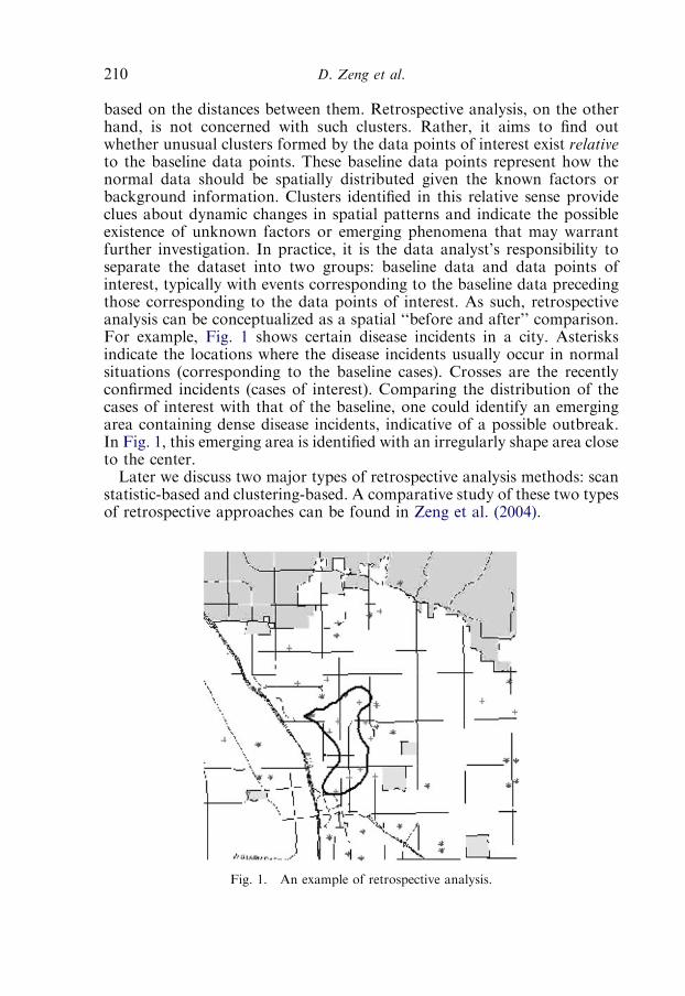
based on the distances between them. Retrospective analysis, on the otherhand, is not concerned with such clusters. Rather, it aims to find outwhether unusual clusters formed by the data points of interest exist relativeto the baseline data points. These baseline data points represent how thenormal data should be spatially distributed given the known factors orbackground information. Clusters identified in this relative sense provideclues about dynamic changes in spatial patterns and indicate the possibleexistence of unknown factors or emerging phenomena that may warrantfurther investigation. In practice, it is the data analyst’s responsibility toseparate the dataset into two groups: baseline data and data points ofinterest, typically with events corresponding to the baseline data precedingthose corresponding to the data points of interest. As such, retrospectiveanalysis can be conceptualized as a spatial ‘‘before and after’’ comparison.For example, Fig. 1 shows certain disease incidents in a city. Asterisksindicate the locations where the disease incidents usually occur in normalsituations (corresponding to the baseline cases). Crosses are the recentlyconfirmed incidents (cases of interest). Comparing the distribution of thecases of interest with that of the baseline, one could identify an emergingarea containing dense disease incidents, indicative of a possible outbreak.In Fig. 1, this emerging area is identified with an irregularly shape area closeto the center.Later we discuss two major types of retrospective analysis methods: scan
statistic-based and clustering-based. A comparative study of these two typesof retrospective approaches can be found in Zeng et al. (2004).
Fig. 1. An example of retrospective analysis.
D. Zeng et al.210
2.1.1.1 Scan statistic-based retrospective analysis. Various types of scanstatistics have been developed in the past four decades for surveillance andmonitoring purposes in a wide range of application contexts. For spatial-temporal data analysis, a representative method is the spatial scan statisticapproach (Kulldorff, 1997). This method has become one of the mostpopular methods for detection of geographical disease clusters and is beingwidely used by public health departments and researchers. In this approach,the number of events, for example, disease cases, may be assumed to beeither Poisson or Bernoulli distributed. Algorithmically, the spatial scanstatistic method imposes a circular window on the map under study and letsthe center of the circle move over the area so that at different positions thewindow includes different sets of neighboring cases. Over the course of dataanalysis, the method creates a large number of distinct circular windows(other shapes such as rectangular and ellipse have also been used), each witha different set of neighboring areas within it and each a possible candidatefor containing an unusual cluster of events. A likelihood ratio is defined oneach circle to compute how likely the cases of interest fall into that circle notby pure chance. The circles with high likelihood ratios are in turn reportedas spatial anomalies or hotspots.
2.1.1.2 Clustering-based retrospective analysis. Despite the success ofthe spatial scan statistic and its variations in spatial anomaly detection, themajor computational problems faced by this type of methods is that thescanning windows are limited to simple, fixed symmetrical shapes foranalytical and search efficiency reasons. As a result, when the realunderlying clusters do not conform to such shapes, the identified regionsare often not well localized. Another problem is that it is often difficult tocustomize and fine-tune the clustering results using scan statisticapproaches. For different types of analysis, the users often have differentneeds as to the level of granularity and the number of the resulting clusters,and they have different degrees of tolerance regarding outliers. Theseproblems have motivated the use of alternative modeling approachesbased on clustering. Risk-adjusted nearest neighbor hierarchical clustering(RNNH) (Levine, 2002) is a representative of such approaches. Developedfor crime hotspot analysis, RNNH is based on the well-known nearestneighbor hierarchical (NNH) clustering method, combining the hierarchicalclustering (Johnson, 1967) capabilities with kernel density interpolationtechniques (Levine, 2002). The standard NNH approach identifies clustersof data points that are close together (based on a threshold distance).Many such clusters, however, are due to some background or baselinefactors (e.g., the population which is not evenly distributed over the entirearea of interest). RNNH is primarily motivated to identify clusters of datapoints relative to the baseline factor. Algorithmically, it dynamically adjuststhe threshold distance inversely proportional to some density measure ofthe baseline factor (e.g., the threshold should be shorter in regions where
Ch. 8. Spatial-Temporal Data Analysis 211
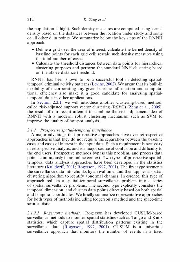
the population is high). Such density measures are computed using kerneldensity based on the distances between the location under study and someor all other data points. We summarize below the key steps of the RNNHapproach.
� Define a grid over the area of interest; calculate the kernel density ofbaseline points for each grid cell; rescale such density measures usingthe total number of cases.� Calculate the threshold distances between data points for hierarchicalclustering purposes and perform the standard NNH clustering basedon the above distance threshold.
RNNH has been shown to be a successful tool in detecting spatial-temporal criminal activity patterns (Levine, 2002). We argue that its built-inflexibility of incorporating any given baseline information and computa-tional efficiency also make it a good candidate for analyzing spatial-temporal data in other applications.In Section 2.2.1, we will introduce another clustering-based method,
called risk-adjusted support vector clustering (RSVC) (Zeng et al., 2005),the result of our recent attempt to combine the risk adjustment idea ofRNNH with a modern, robust clustering mechanism such as SVM toimprove the quality of hotspot analysis.
2.1.2 Prospective spatial-temporal surveillanceA major advantage that prospective approaches have over retrospective
approaches is that they do not require the separation between the baselinecases and cases of interest in the input data. Such a requirement is necessaryin retrospective analysis, and is a major source of confusion and difficulty tothe end users. Prospective methods bypass this problem, and process datapoints continuously in an online context. Two types of prospective spatial-temporal data analysis approaches have been developed in the statisticsliterature (Kulldorff, 2001; Rogerson, 1997, 2001). The first type segmentsthe surveillance data into chunks by arrival time, and then applies a spatialclustering algorithm to identify abnormal changes. In essence, this type ofapproach reduces a spatial-temporal surveillance problem into a seriesof spatial surveillance problems. The second type explicitly considers thetemporal dimension, and clusters data points directly based on both spatialand temporal coordinates. We briefly summarize representative approachesfor both types of methods including Rogerson’s method and the space-timescan statistic.
2.1.2.1 Rogerson’s methods. Rogerson has developed CUSUM-basedsurveillance methods to monitor spatial statistics such as Tango and Knoxstatistics, which capture spatial distribution patterns existing in thesurveillance data (Rogerson, 1997, 2001). CUSUM is a univariatesurveillance approach that monitors the number of events in a fixed
D. Zeng et al.212
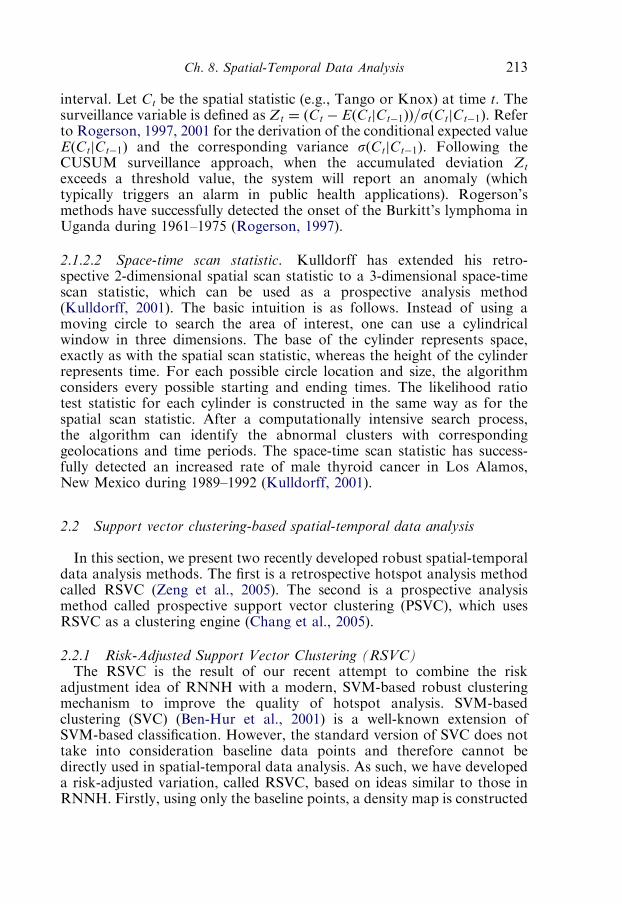
interval. Let Ct be the spatial statistic (e.g., Tango or Knox) at time t. Thesurveillance variable is defined as Zt ¼ ðCt � EðCtjCt�1ÞÞ=sðCtjCt�1Þ. Referto Rogerson, 1997, 2001 for the derivation of the conditional expected valueEðCtjCt�1Þ and the corresponding variance sðCtjCt�1Þ. Following theCUSUM surveillance approach, when the accumulated deviation Zt
exceeds a threshold value, the system will report an anomaly (whichtypically triggers an alarm in public health applications). Rogerson’smethods have successfully detected the onset of the Burkitt’s lymphoma inUganda during 1961–1975 (Rogerson, 1997).
2.1.2.2 Space-time scan statistic. Kulldorff has extended his retro-spective 2-dimensional spatial scan statistic to a 3-dimensional space-timescan statistic, which can be used as a prospective analysis method(Kulldorff, 2001). The basic intuition is as follows. Instead of using amoving circle to search the area of interest, one can use a cylindricalwindow in three dimensions. The base of the cylinder represents space,exactly as with the spatial scan statistic, whereas the height of the cylinderrepresents time. For each possible circle location and size, the algorithmconsiders every possible starting and ending times. The likelihood ratiotest statistic for each cylinder is constructed in the same way as for thespatial scan statistic. After a computationally intensive search process,the algorithm can identify the abnormal clusters with correspondinggeolocations and time periods. The space-time scan statistic has success-fully detected an increased rate of male thyroid cancer in Los Alamos,New Mexico during 1989–1992 (Kulldorff, 2001).
2.2 Support vector clustering-based spatial-temporal data analysis
In this section, we present two recently developed robust spatial-temporaldata analysis methods. The first is a retrospective hotspot analysis methodcalled RSVC (Zeng et al., 2005). The second is a prospective analysismethod called prospective support vector clustering (PSVC), which usesRSVC as a clustering engine (Chang et al., 2005).
2.2.1 Risk-Adjusted Support Vector Clustering (RSVC)The RSVC is the result of our recent attempt to combine the risk
adjustment idea of RNNH with a modern, SVM-based robust clusteringmechanism to improve the quality of hotspot analysis. SVM-basedclustering (SVC) (Ben-Hur et al., 2001) is a well-known extension ofSVM-based classification. However, the standard version of SVC does nottake into consideration baseline data points and therefore cannot bedirectly used in spatial-temporal data analysis. As such, we have developeda risk-adjusted variation, called RSVC, based on ideas similar to those inRNNH. Firstly, using only the baseline points, a density map is constructed
Ch. 8. Spatial-Temporal Data Analysis 213

using standard approaches such as the kernel density estimation method.Secondly, the case data points are mapped implicitly to a high-dimensionalfeature space defined by a kernel function (typically the Gaussian kernel).The width parameter in the Gaussian kernel function determines thedimensionality of the feature space. The larger the width parameter is, theharder the data points in the original space constitute a cluster and hencedata points are more likely to belong to smaller clusters. Our algorithmdynamically adjusts the width parameter based on the kernel densityestimates obtained in the previous step. The basic intuition is as follows:when the baseline density is high, a larger width value is used to make itharder for points to be clustered together. Thirdly, following the SVMapproach, RSVC finds a hypersphere in the feature space with a minimalradius to contain most of the data. The problem of finding this hyperspherecan be formulated as a quadratic or linear program depending on thedistance function used. Fourthly, the function estimating the supportof the underlying data distribution is then constructed using the kernelfunction and the parameters learned in the third step. When projectedback to the original data space, the identified hypersphere is mapped to(possibly multiple) clusters. These clusters are then returned as the outputof RSVC.
2.2.2 Prospective support vector clusteringAlthough well-grounded in theoretical development, both Rogerson’s
methods and the space–time scan statistic have major computationalproblems. Rogerson’s approaches can monitor a given target area butcannot search for problematic areas or identify the geographic shape ofthese areas. The space–time scan statistic method performs poorly when thetrue abnormal areas do not conform to simple shapes such as circles. Belowwe introduce the basic ideas behind our approach, which is called PSVC,and summarize its main algorithmic steps.Our PSVC approach follows the design of the first type of the spatial-
temporal surveillance method discussed in Section 2.2, which involvesrepeated spatial clusterings over time. More specifically, the time horizonis first discretized based on the specific characteristics of the data streamunder study. Whenever a new batch of data arrives, PSVC treats thedata collected during the previous time frame as the baseline data, andruns the retrospective RSVC method. After obtaining a potential abnormalarea, PSVC attempts to determine how statistically significant theidentified spatial anomaly is. Many indices have been developed to assessthe significance of the results of clustering algorithms in general (Halkidiet al., 2002a,b). However, all these criteria assess clustering in anabsolute sense without considering the baseline information. Thus, theyare not readily suitable for prospective spatial-temporal data analysis.Kulldorff’s (1997) likelihood ratio L(Z) as defined in the followingequation is to our best knowledge the only statistic that explicitly takes
D. Zeng et al.214

the baseline information into account.
LðZÞ ¼c
n
� �c1�
c
n
� �n�c C � c
N � n
� �C�c
1�C � c
N � n
� �ðN�nÞ�ðC�cÞ(1)
In this definition, C and c are the number of the cases in the entire datasetand the number of the cases within the scanned area Z, respectively. N andn are the total number of the cases and the baseline points in the entiredataset and the total number of the cases and the baseline points within Z,respectively. Since the distribution of the statistic L(Z) is unknown, weuse the standard simulation approach to calculate statistical significancemeasured by the p-value. Specifically, we first generate T replications of thedataset, assuming that the data are randomly distributed. We then calculatethe likelihood ratio L(Z) in the same area Z for each replication. Finally, werank these likelihood ratios and if L takes the Xth position, then the p-valueis set to be X/(Tþ1).Note that in a straightforward implementation of the earlier algorithmic
design, anomalies are identified (or equivalently alerts are triggered) onlywhen adjacent data batches have significant changes in terms of dataspatial distribution. This localized myopic view, however, may lead tosignificant delay in alarm triggering or even false negatives because in somecircumstances, unusual changes may manifest gradually. In such cases,there might not be any significant changes between adjacent data batches.However, the accumulated changes over several consecutive batches can besignificant and should trigger an alarm. This observation suggests that amore ‘‘global’’ perspective beyond comparing adjacent data batches isneeded. It turns out that the CUSUM approach provides a suitableconceptual framework to help design a computational approach with such aglobal perspective. The analogy is as follows. In the CUSUM approach,accumulative deviations from the expected value are explicitly kept track of.In prospective analysis, it is difficult to design a single one-dimensionalstatistic to capture what the normal spatial distribution should looklike and to measure the extent to which deviations occur. However,conceptually the output of a retrospective surveillance method such asRSVC can be viewed as the differences or discrepancies between two databatches, with the baseline data representing the expected data distribution.In addition, accumulative discrepancies can be computed by running RSVCwith properly set baseline and case data separation. For an efficientimplementation, we use a stack as a control data structure to keeptrack of RSVC runs which now include comparisons beyond data fromadjacent single periods. The detailed control strategy is described later.When clusters generated in two consecutive RSVC runs have overlaps, wedeem that the areas covered by these clusters are risky areas. We use thestack to store the clusters along with the data batches from which theserisky clusters are identified. Then we run RSVC to compare the current data
Ch. 8. Spatial-Temporal Data Analysis 215

batch with each element (in the form of a data batch) of the stacksequentially from the top to the bottom to examine whether significantspatial pattern changes have occurred. Stacks whose top data batch is notthe current data batch under examination can be emptied since the areasrepresented by them no longer have the trend to bring on any significantdistribution change. This operation resembles one of the steps in theCUSUM calculation where the accumulated deviation is reset to 0 when themonitored variable is no longer within the risky range.We now explain the main steps of the PSVC algorithm as shown in Fig. 2.
Each cluster stack represents a candidate abnormal area and the arrayclusterstacks holds a number of cluster stacks keeping track of all candidateareas at stake. Initially (line 1) clusterstacks is empty. The steps from line 3to 35 are run whenever a new data batch enters the system. First, the RSVCretrospective method is executed (line 3) to compare the spatial distributionof the new data batch with that of the previous data batch. The resultingabnormal clusters are saved in rsvcresult. Any statistically significant clusterin rsvcresult will immediately trigger an alert (line 5).
1 clusterstacks=[] 2 Whenever a new data batch arrives { 3 rsvcresult=RSVC (previousdate, currentdate)4 For each cluster C recorded in rsvcresult {
/*C records the identified cluster, its p-value, and the date of the associated data batch. */ 5 If (C.p-value<threshold) {Trigger alert} 6 Else { 7 If (clusterstacks is not empty) { 8 For each cluster stack S in clusterstacks {9 lastcluster=the top element of the stack S10 If cluster C has overlaps with lastcluster {11 S.append(C)12 For each element in the stack S from top to bottom { 13 tempresult=RSVC (element.date, currentdate)14 For each temporal cluster TC recorded in tempresult {15 if (TC.p-value<threshold) {Trigger alert} 16 } 17 } 18 } 19 } 20 If (current cluster C does not have any overlap 21 with any of the top element of the clusters in clusterstacks) { 22 new stack NS=[C]23 clusterstacks.append(NS)24 } 25 For each cluster stack S { 26 If (S[top element].date!=currentdate) {delete stack S}27 } 28 } 29 Else { 30 new stack NS=[C]31 clusterstacks.append(NS)32 } 33 } 34 } 35}
Fig. 2. PSVC algorithm.
D. Zeng et al.216
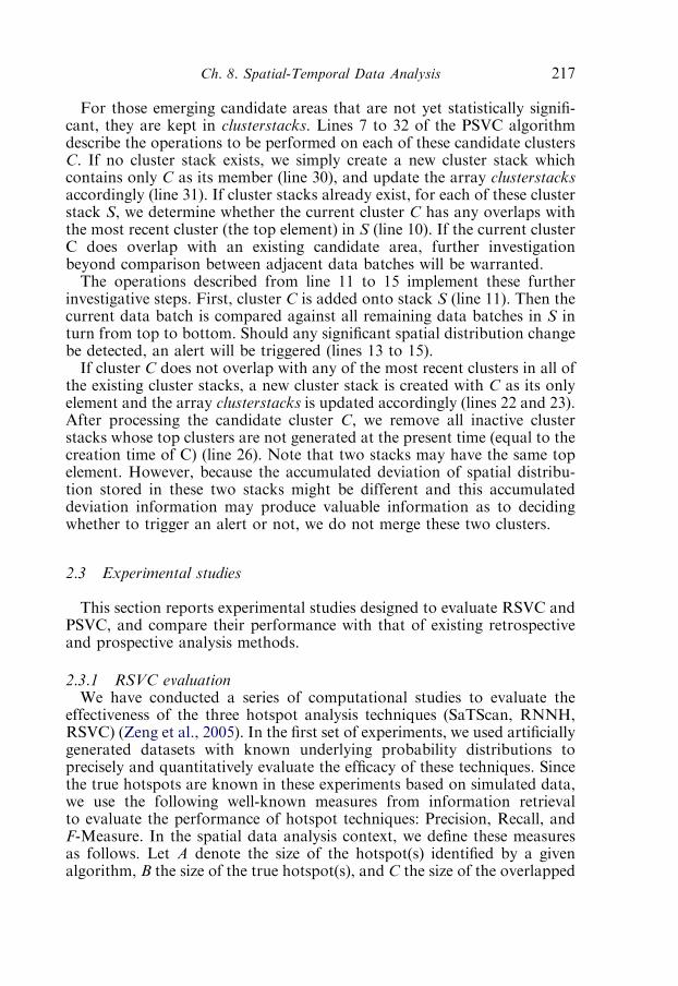
For those emerging candidate areas that are not yet statistically signifi-cant, they are kept in clusterstacks. Lines 7 to 32 of the PSVC algorithmdescribe the operations to be performed on each of these candidate clustersC. If no cluster stack exists, we simply create a new cluster stack whichcontains only C as its member (line 30), and update the array clusterstacksaccordingly (line 31). If cluster stacks already exist, for each of these clusterstack S, we determine whether the current cluster C has any overlaps withthe most recent cluster (the top element) in S (line 10). If the current clusterC does overlap with an existing candidate area, further investigationbeyond comparison between adjacent data batches will be warranted.The operations described from line 11 to 15 implement these further
investigative steps. First, cluster C is added onto stack S (line 11). Then thecurrent data batch is compared against all remaining data batches in S inturn from top to bottom. Should any significant spatial distribution changebe detected, an alert will be triggered (lines 13 to 15).If cluster C does not overlap with any of the most recent clusters in all of
the existing cluster stacks, a new cluster stack is created with C as its onlyelement and the array clusterstacks is updated accordingly (lines 22 and 23).After processing the candidate cluster C, we remove all inactive clusterstacks whose top clusters are not generated at the present time (equal to thecreation time of C) (line 26). Note that two stacks may have the same topelement. However, because the accumulated deviation of spatial distribu-tion stored in these two stacks might be different and this accumulateddeviation information may produce valuable information as to decidingwhether to trigger an alert or not, we do not merge these two clusters.
2.3 Experimental studies
This section reports experimental studies designed to evaluate RSVC andPSVC, and compare their performance with that of existing retrospectiveand prospective analysis methods.
2.3.1 RSVC evaluationWe have conducted a series of computational studies to evaluate the
effectiveness of the three hotspot analysis techniques (SaTScan, RNNH,RSVC) (Zeng et al., 2005). In the first set of experiments, we used artificiallygenerated datasets with known underlying probability distributions toprecisely and quantitatively evaluate the efficacy of these techniques. Sincethe true hotspots are known in these experiments based on simulated data,we use the following well-known measures from information retrievalto evaluate the performance of hotspot techniques: Precision, Recall, andF-Measure. In the spatial data analysis context, we define these measuresas follows. Let A denote the size of the hotspot(s) identified by a givenalgorithm, B the size of the true hotspot(s), and C the size of the overlapped
Ch. 8. Spatial-Temporal Data Analysis 217
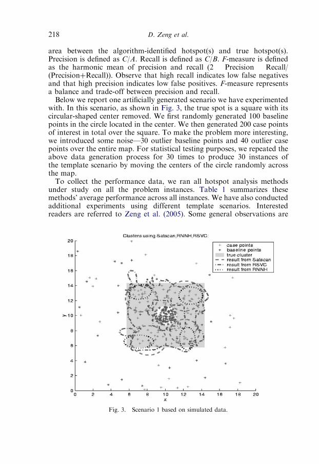
area between the algorithm-identified hotspot(s) and true hotspot(s).Precision is defined as C/A. Recall is defined as C/B. F-measure is definedas the harmonic mean of precision and recall (2 � Precision � Recall/(PrecisionþRecall)). Observe that high recall indicates low false negativesand that high precision indicates low false positives. F-measure representsa balance and trade-off between precision and recall.Below we report one artificially generated scenario we have experimented
with. In this scenario, as shown in Fig. 3, the true spot is a square with itscircular-shaped center removed. We first randomly generated 100 baselinepoints in the circle located in the center. We then generated 200 case pointsof interest in total over the square. To make the problem more interesting,we introduced some noise—30 outlier baseline points and 40 outlier casepoints over the entire map. For statistical testing purposes, we repeated theabove data generation process for 30 times to produce 30 instances ofthe template scenario by moving the centers of the circle randomly acrossthe map.To collect the performance data, we ran all hotspot analysis methods
under study on all the problem instances. Table 1 summarizes thesemethods’ average performance across all instances. We have also conductedadditional experiments using different template scenarios. Interestedreaders are referred to Zeng et al. (2005). Some general observations are
Fig. 3. Scenario 1 based on simulated data.
D. Zeng et al.218
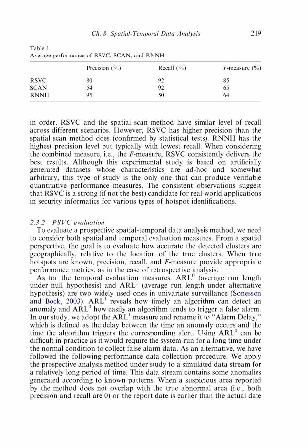
in order. RSVC and the spatial scan method have similar level of recallacross different scenarios. However, RSVC has higher precision than thespatial scan method does (confirmed by statistical tests). RNNH has thehighest precision level but typically with lowest recall. When consideringthe combined measure, i.e., the F-measure, RSVC consistently delivers thebest results. Although this experimental study is based on artificiallygenerated datasets whose characteristics are ad-hoc and somewhatarbitrary, this type of study is the only one that can produce verifiablequantitative performance measures. The consistent observations suggestthat RSVC is a strong (if not the best) candidate for real-world applicationsin security informatics for various types of hotspot identifications.
2.3.2 PSVC evaluationTo evaluate a prospective spatial-temporal data analysis method, we need
to consider both spatial and temporal evaluation measures. From a spatialperspective, the goal is to evaluate how accurate the detected clusters aregeographically, relative to the location of the true clusters. When truehotspots are known, precision, recall, and F-measure provide appropriateperformance metrics, as in the case of retrospective analysis.As for the temporal evaluation measures, ARL0 (average run length
under null hypothesis) and ARL1 (average run length under alternativehypothesis) are two widely used ones in univariate surveillance (Sonessonand Bock, 2003). ARL1 reveals how timely an algorithm can detect ananomaly and ARL0 how easily an algorithm tends to trigger a false alarm.In our study, we adopt the ARL1 measure and rename it to ‘‘Alarm Delay,’’which is defined as the delay between the time an anomaly occurs and thetime the algorithm triggers the corresponding alert. Using ARL0 can bedifficult in practice as it would require the system run for a long time underthe normal condition to collect false alarm data. As an alternative, we havefollowed the following performance data collection procedure. We applythe prospective analysis method under study to a simulated data stream fora relatively long period of time. This data stream contains some anomaliesgenerated according to known patterns. When a suspicious area reportedby the method does not overlap with the true abnormal area (i.e., bothprecision and recall are 0) or the report date is earlier than the actual date
Table 1
Average performance of RSVC, SCAN, and RNNH
Precision (%) Recall (%) F-measure (%)
RSVC 80 92 85
SCAN 54 92 65
RNNH 95 50 64
Ch. 8. Spatial-Temporal Data Analysis 219
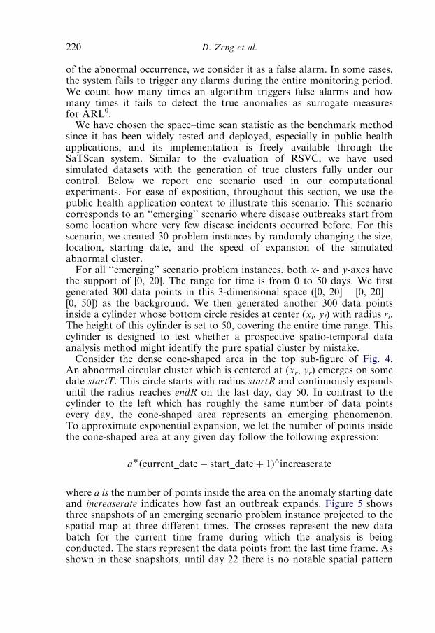
of the abnormal occurrence, we consider it as a false alarm. In some cases,the system fails to trigger any alarms during the entire monitoring period.We count how many times an algorithm triggers false alarms and howmany times it fails to detect the true anomalies as surrogate measuresfor ARL0.We have chosen the space–time scan statistic as the benchmark method
since it has been widely tested and deployed, especially in public healthapplications, and its implementation is freely available through theSaTScan system. Similar to the evaluation of RSVC, we have usedsimulated datasets with the generation of true clusters fully under ourcontrol. Below we report one scenario used in our computationalexperiments. For ease of exposition, throughout this section, we use thepublic health application context to illustrate this scenario. This scenariocorresponds to an ‘‘emerging’’ scenario where disease outbreaks start fromsome location where very few disease incidents occurred before. For thisscenario, we created 30 problem instances by randomly changing the size,location, starting date, and the speed of expansion of the simulatedabnormal cluster.For all ‘‘emerging’’ scenario problem instances, both x- and y-axes have
the support of [0, 20]. The range for time is from 0 to 50 days. We firstgenerated 300 data points in this 3-dimensional space ([0, 20] � [0, 20] �
[0, 50]) as the background. We then generated another 300 data pointsinside a cylinder whose bottom circle resides at center (xl, yl) with radius rl.The height of this cylinder is set to 50, covering the entire time range. Thiscylinder is designed to test whether a prospective spatio-temporal dataanalysis method might identify the pure spatial cluster by mistake.Consider the dense cone-shaped area in the top sub-figure of Fig. 4.
An abnormal circular cluster which is centered at (xr, yr) emerges on somedate startT. This circle starts with radius startR and continuously expandsuntil the radius reaches endR on the last day, day 50. In contrast to thecylinder to the left which has roughly the same number of data pointsevery day, the cone-shaped area represents an emerging phenomenon.To approximate exponential expansion, we let the number of points insidethe cone-shaped area at any given day follow the following expression:
a n ðcurrent_date� start_dateþ 1Þ^increaserate
where a is the number of points inside the area on the anomaly starting dateand increaserate indicates how fast an outbreak expands. Figure 5 showsthree snapshots of an emerging scenario problem instance projected to thespatial map at three different times. The crosses represent the new databatch for the current time frame during which the analysis is beingconducted. The stars represent the data points from the last time frame. Asshown in these snapshots, until day 22 there is no notable spatial pattern
D. Zeng et al.220

change during two consecutive weeks. But during the week from day 22 today 29, we can clearly observe an emerging circle.When generating data points for 30 replications of the emerging scenario,
we aimed to experiment with the cone-shaped area and the cylinder of
05
1015
20
0
5
10
15
200
10
20
30
40
50
x
"emerging" scenario data set
y
z
0 5 10 15 200
2
4
6
8
10
12
14
16
18
20
x
y
Emerging anomaly detected on day 29 ("emerging" scenario)
incidents collected on day 22incidents collected on day 29PSVC resultSatScan resulttrue cluster
Fig. 4. A problem instance of the ‘‘emerging’’ scenario.
Ch. 8. Spatial-Temporal Data Analysis 221
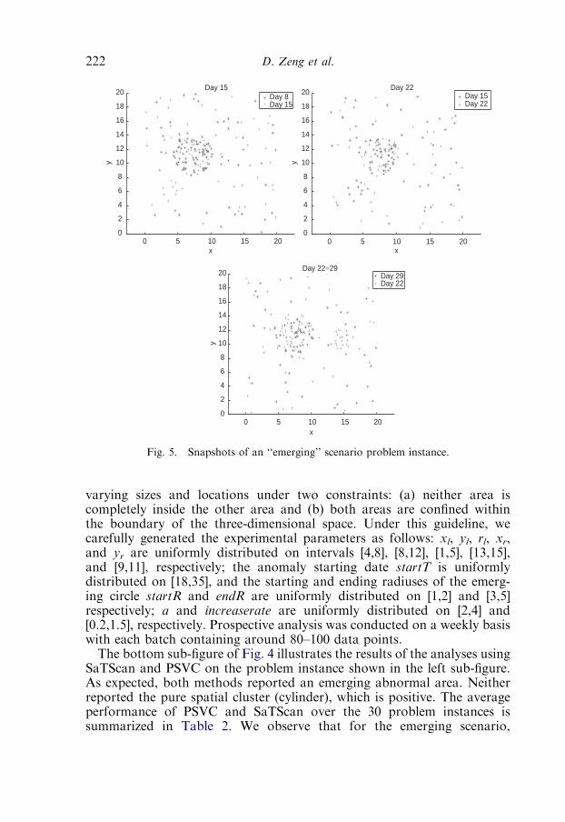
varying sizes and locations under two constraints: (a) neither area iscompletely inside the other area and (b) both areas are confined withinthe boundary of the three-dimensional space. Under this guideline, wecarefully generated the experimental parameters as follows: xl, yl, rl, xr,and yr are uniformly distributed on intervals [4,8], [8,12], [1,5], [13,15],and [9,11], respectively; the anomaly starting date startT is uniformlydistributed on [18,35], and the starting and ending radiuses of the emerg-ing circle startR and endR are uniformly distributed on [1,2] and [3,5]respectively; a and increaserate are uniformly distributed on [2,4] and[0.2,1.5], respectively. Prospective analysis was conducted on a weekly basiswith each batch containing around 80–100 data points.The bottom sub-figure of Fig. 4 illustrates the results of the analyses using
SaTScan and PSVC on the problem instance shown in the left sub-figure.As expected, both methods reported an emerging abnormal area. Neitherreported the pure spatial cluster (cylinder), which is positive. The averageperformance of PSVC and SaTScan over the 30 problem instances issummarized in Table 2. We observe that for the emerging scenario,
0 5 10 15 200
2
4
6
8
10
12
14
16
18
20
x
y
Day 15Day 8Day 15
x0 5 10 15 20
0
2
4
6
8
10
12
14
16
18
20
y
Day 22Day 15Day 22
0 5 10 15 200
2
4
6
8
10
12
14
16
18
20
x
y
Day 22−29Day 29Day 22
Fig. 5. Snapshots of an ‘‘emerging’’ scenario problem instance.
D. Zeng et al.222
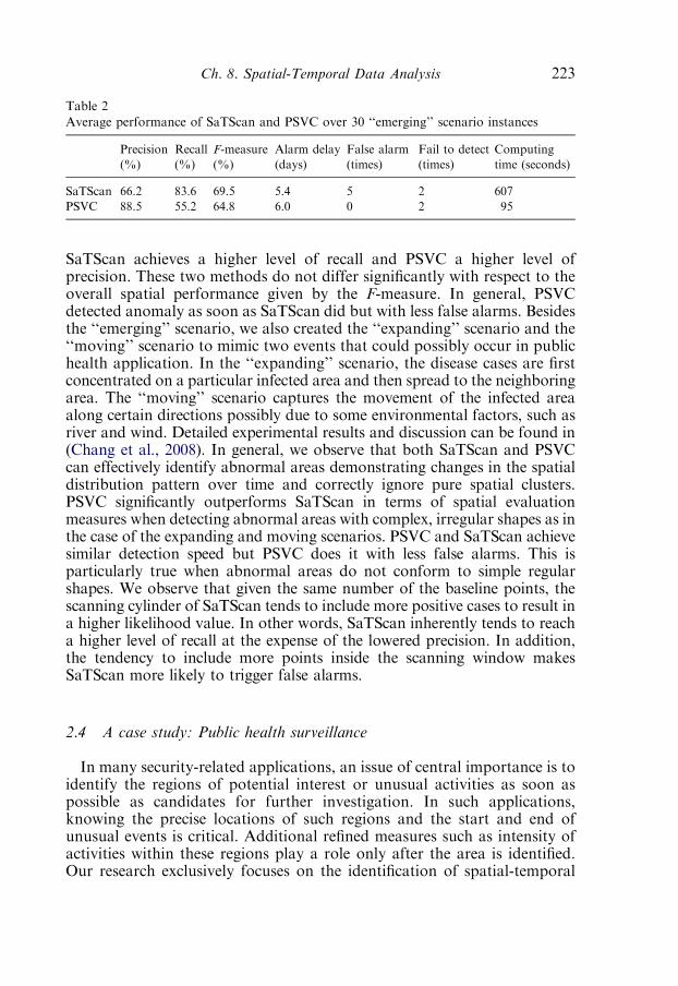
SaTScan achieves a higher level of recall and PSVC a higher level ofprecision. These two methods do not differ significantly with respect to theoverall spatial performance given by the F-measure. In general, PSVCdetected anomaly as soon as SaTScan did but with less false alarms. Besidesthe ‘‘emerging’’ scenario, we also created the ‘‘expanding’’ scenario and the‘‘moving’’ scenario to mimic two events that could possibly occur in publichealth application. In the ‘‘expanding’’ scenario, the disease cases are firstconcentrated on a particular infected area and then spread to the neighboringarea. The ‘‘moving’’ scenario captures the movement of the infected areaalong certain directions possibly due to some environmental factors, such asriver and wind. Detailed experimental results and discussion can be found in(Chang et al., 2008). In general, we observe that both SaTScan and PSVCcan effectively identify abnormal areas demonstrating changes in the spatialdistribution pattern over time and correctly ignore pure spatial clusters.PSVC significantly outperforms SaTScan in terms of spatial evaluationmeasures when detecting abnormal areas with complex, irregular shapes as inthe case of the expanding and moving scenarios. PSVC and SaTScan achievesimilar detection speed but PSVC does it with less false alarms. This isparticularly true when abnormal areas do not conform to simple regularshapes. We observe that given the same number of the baseline points, thescanning cylinder of SaTScan tends to include more positive cases to result ina higher likelihood value. In other words, SaTScan inherently tends to reacha higher level of recall at the expense of the lowered precision. In addition,the tendency to include more points inside the scanning window makesSaTScan more likely to trigger false alarms.
2.4 A case study: Public health surveillance
In many security-related applications, an issue of central importance is toidentify the regions of potential interest or unusual activities as soon aspossible as candidates for further investigation. In such applications,knowing the precise locations of such regions and the start and end ofunusual events is critical. Additional refined measures such as intensity ofactivities within these regions play a role only after the area is identified.Our research exclusively focuses on the identification of spatial-temporal
Table 2
Average performance of SaTScan and PSVC over 30 ‘‘emerging’’ scenario instances
Precision
(%)
Recall
(%)
F-measure
(%)
Alarm delay
(days)
False alarm
(times)
Fail to detect
(times)
Computing
time (seconds)
SaTScan 66.2 83.6 69.5 5.4 5 2 607
PSVC 88.5 55.2 64.8 6.0 0 2 95
Ch. 8. Spatial-Temporal Data Analysis 223
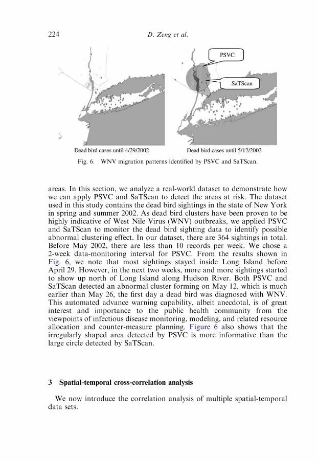
areas. In this section, we analyze a real-world dataset to demonstrate howwe can apply PSVC and SaTScan to detect the areas at risk. The datasetused in this study contains the dead bird sightings in the state of New Yorkin spring and summer 2002. As dead bird clusters have been proven to behighly indicative of West Nile Virus (WNV) outbreaks, we applied PSVCand SaTScan to monitor the dead bird sighting data to identify possibleabnormal clustering effect. In our dataset, there are 364 sightings in total.Before May 2002, there are less than 10 records per week. We chose a2-week data-monitoring interval for PSVC. From the results shown inFig. 6, we note that most sightings stayed inside Long Island beforeApril 29. However, in the next two weeks, more and more sightings startedto show up north of Long Island along Hudson River. Both PSVC andSaTScan detected an abnormal cluster forming on May 12, which is muchearlier than May 26, the first day a dead bird was diagnosed with WNV.This automated advance warning capability, albeit anecdotal, is of greatinterest and importance to the public health community from theviewpoints of infectious disease monitoring, modeling, and related resourceallocation and counter-measure planning. Figure 6 also shows that theirregularly shaped area detected by PSVC is more informative than thelarge circle detected by SaTScan.
3 Spatial-temporal cross-correlation analysis
We now introduce the correlation analysis of multiple spatial-temporaldata sets.
Fig. 6. WNV migration patterns identified by PSVC and SaTScan.
D. Zeng et al.224

3.1 Literature review
In general, correlation refers to the departure of two random eventsfrom independence. In the specific area of spatial-temporal data analysis,correlation is to measure the degree of co-existing of multiple dataobservations in a close geographical neighborhood and a short timeframe. In this section, we use the ‘‘data event’’ to represent one type of datastream, and the ‘‘data observation’’ to represent one occurrence of a dataevent. For example, in infectious disease informatics, a data event can be‘‘dead birds,’’ and a data observation is a specific occurrence of dead birds.Depending on the co-existing effect among data observations, there are
two possible types of correlations (Dixon, 2002). Positive correlationindicates that an observation increases the probability of other observationsto occur, whereas negative correlation indicates that an observation tendsto decrease the appearance probability of other observations. In the domainof infectious disease informatics, if a dead bird occurrence tends to increasethe probability of more dead birds to occur, we state that the event of deadbirds has a positive correlation to itself.With respect to the number of data events being analyzed, two types of
correlation analyses can be defined (Ripley, 1981). If the observations ofone data event are not independent, the event is called auto-correlated.If the observations of one event are not independent of those of anotherevent, those two events are cross-correlated. This section is mainlyconcerned with the cross-correlations.Depending on the type of data being analyzed, correlation analysis can be
categorized into time-series correlation, spatial correlation, and spatial-temporal correlation. We will briefly summarize the literature on all thesethree types of correlations. Our research is particularly interested in theanalysis of spatial-temporal cross-correlations. Specifically we are interestedin exploring the possible correlations among events by studying therelations of the geographical locations and the time of the observations.
3.1.1 Time series cross-correlationsTime series cross-correlation analysis focuses on the correlation of
multiple data events with temporal components. The methods to analyzetime series cross-correlations are well established and are generally availablein commercial statistical software packages.Two representative studies from the public health informatics are
summarized below.Lean et al. (1992) used time series cross-correlation analysis to determine
relationships among glucose, cholesterol, and milk yield, for 42 dayspostpartum for 14 multiparous cows. They claimed that time series cross-correlation analysis was a useful tool in examining relationships amongvariables when repeated samples were obtained from the same individuals.
Ch. 8. Spatial-Temporal Data Analysis 225

Cappaert et al. (1991) used time series cross-correlation to estimatesynchrony of Colorado potato beetle eggs with predators. Predators,including asopine pentatomids, carabids, thomisid spiders, and coccinellids,were abundant and well synchronized with developing Colorado potatobeetle in late 1987, corresponding to the period of highest mortality.
3.1.2 Moran’s IA widely adopted statistical measure in spatial correlation analysis is
Moran’s I index (Moran, 1948). Moran’s I is a weighted correlationcoefficient used to detect departures from spatial randomness. Departuresfrom randomness indicate spatial patterns, such as clusters. The statisticmay identify other kinds of patterns such as the geographic trend. The valueof Moran’s I can be from �1 to 1. Values of I larger than 0 indicate positivespatial correlation; values smaller than 0 indicate negative spatialcorrelation. Moran’s I is commonly applied in areas such as epidemiologyand many extensions have been developed (Thioulouse et al., 1995;Waldhor, 1996). Moran’s I requires a comparable numeric value for eachobservation (e.g., a count of a certain event), and is not suitable for dataanalysis in which data observations only have information about theoccurring location and time.
3.1.3 Ripley’s K(r)Ripley’s K(r) function is a tool for analyzing completely mapped spatial
point process data, i.e., the locations of data observations in a predefinedstudy area. Ripley’s K(r) function can be used to summarize a point pattern,and test hypotheses about the pattern. Bivariate generalizations can be usedto describe correlative relationships between two point patterns. Applica-tions include spatial patterns of trees (Peterson and Squiers, 1995; Stoyanand Penttinen, 2000), bird nests (Gaines et al., 2000), and disease cases(Diggle and Chetwynd, 1991). Details of various theoretical aspects of K(r)are in books by (Diggle et al., 1976; Dixon, 2002; Ripley, 1981).Formally, the K(r) function is defined as
KijðrÞ ¼ l�1j E ðNumber of event j observations within distance rof a randomly chosen event i observationÞ ð2Þ
In Eq. (2) (Ripley, 1976), lj is the density (the number of observations perunit area) of event j. The higher the K(r) value, the stronger the correlationis. When i ¼ j, the value of K(r) indicates the auto-correlative magnitude.Given the locations of all data observations of all data events, K(r) can be
estimated as follows (Ripley, 1976).
K ijðrÞ ¼1
liljA
Xim
Xjn
wðim; jnÞIðdim; jnorÞ (3)
D. Zeng et al.226

A is the area of the study region. The unbiased estimated density lj isgiven by Number of Observations of Event j/A. In Eq. (3), im denotes them-th observation of event i, and dim; jn the distance between im and jn. I(x) isan indicator variable whose value is 1 when x is true and 0 otherwise.The term wðim; jnÞ takes into account of the edge effect. The edge effectconsiders the situation where im is so close to the edge of the studyregion that the impact of im on jn should be discounted. The value ofwðim; jnÞ is the fraction of the circumference of a circle centered at imwith radius dim; jn that lies inside the study region. From Eq. (3) the value ofK(r) function ranges from zero to the area A if the edge effect is ignored(Ripley, 1976).While the traditional Ripley’s K(r) function has been proven effective
in discovering spatial cross-correlative relations, it does not include thetemporal component. Simply considering spatial condition and ignoringtemporal effect will possibly lead to false conclusions in many applica-tions. Take a common scenario in infectious disease informatics asan example. A recent dead bird observation is unlikely to be related toanother observation that happened 10 years ago in a close spatialneighborhood. However, based on Eq. (3), Iðdim; jnorÞ has the value 1as far as those two observations occurred in a close neighborhood.More specifically, Ripley’s K(r) function has two effects that may leadto false conclusions of cross-correlations. We now discuss them byexamples.The first effect is what we refer to as the ‘‘aggregate effect’’ which may
overlook significant correlations under certain circumstances. A typicalscenario of positive correlations in infectious disease informatics is that adisease case has positive effects within its neighborhood in a short period oftime. As time passes, the effects decrease, and disappear eventually. Forexample, given an observation im, assume that there were many occurrencesin the neighborhood in the next 30 days after im happened, but fewoccurrences in other time periods in the same neighborhood. The absence ofoccurrences at other time periods could dilute the intensity of occurrenceswithin the neighborhood. The overall K(r) value may not be high enoughto report a significant correlation even though a real possible positivecorrelation is likely.We define the second effect as the ‘‘backward shadow effect’’ that may
falsely indicate irrational correlations. Given im, assume there were manyoccurrences happened in the neighborhood prior to the time of im, and fewafter im occurred. Since K(r) does not differentiate if the occurrenceshappened before or after the time of im, the abundance of previouslyoccurred observations will play a dominant role. As a result, the overallK(r) value may indicate a significant positive correlation. This conclusion,however, may be false because the correlation is built on the processimplying that previously occurred cases can be affected by casesoccurred later.
Ch. 8. Spatial-Temporal Data Analysis 227

3.2 Extended K(r) function with temporal considerations
To analyze spatial-temporal correlation, we have proposed a newmeasure K(r, t) that extends the traditional Ripley’s K(r) function by con-sidering temporal effects. We intend to reduce the aggregate effect byeliminating the data observations that satisfy the spatial restriction butoccur at time periods that are very far apart. Eq. (4) gives a mathematicaldefinition of our new measure.
Kijðr; tÞ ¼ l�1j E ðNumber of event j observations within distance r and
time t sincea randomly chosen event i observationÞ ð4Þ
Note the density of event j, lj, is defined as the number of observations ofevent j per unit area per time period.Depending on whether or not the backward shadow effect is taken into
account, two types of time windows can be defined. Given a randomlychosen event i occurrence, im, the first type of time window, defined as theone-tail time effect, only considers the data observations occurred after thetime of im. The second type, defined as the two-tail time effect, considersboth before and after the time of im.Eqs. (4) and (5) define the unbiased estimations of K(r, t) using one-tailed
and two-tailed time effects, respectively.
K ijðr; tÞ ¼1
liljAT
Xim
Xjn
wðim; jnÞIðdim; jnor and 0 � tjn � timotÞ (5)
K ijðr; tÞ ¼1
liljAT
Xim
Xjn
wðim; jnÞIðdim; jnor and � totjn � timotÞ (6)
In these definitions, T is the entire time span. The occurring time of jnis defined by tjn . The terms 0 � tjn � timot and �totjn � timot eliminatethose unlikely related observations by restricting the observations within acertain time window around the time of im.Note that K ijðr; tÞ is a monotonically increasing function with respect to
the radius r and time t. The minimum of the function value is 0 and themaximum is the product of the study area A and time span T if the edgeeffect is ignored. Also note that when the time window t is set to be greaterthan the time span T, Eq. (6) provides no more restriction than Eq. (3).Their values only differ by a constant T.On the other hand, even when the time window t is set to be infinite,
Eq. (5) is still different from Eq. (3) because one-tail K(r, t) eliminates thebackward shadow effect.
D. Zeng et al.228
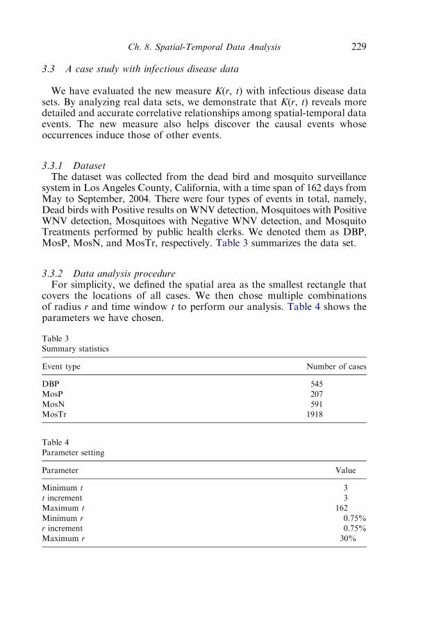
3.3 A case study with infectious disease data
We have evaluated the new measure K(r, t) with infectious disease datasets. By analyzing real data sets, we demonstrate that K(r, t) reveals moredetailed and accurate correlative relationships among spatial-temporal dataevents. The new measure also helps discover the causal events whoseoccurrences induce those of other events.
3.3.1 DatasetThe dataset was collected from the dead bird and mosquito surveillance
system in Los Angeles County, California, with a time span of 162 days fromMay to September, 2004. There were four types of events in total, namely,Dead birds with Positive results on WNV detection, Mosquitoes with PositiveWNV detection, Mosquitoes with Negative WNV detection, and MosquitoTreatments performed by public health clerks. We denoted them as DBP,MosP, MosN, and MosTr, respectively. Table 3 summarizes the data set.
3.3.2 Data analysis procedureFor simplicity, we defined the spatial area as the smallest rectangle that
covers the locations of all cases. We then chose multiple combinationsof radius r and time window t to perform our analysis. Table 4 shows theparameters we have chosen.
Table 3
Summary statistics
Event type Number of cases
DBP 545
MosP 207
MosN 591
MosTr 1918
Table 4
Parameter setting
Parameter Value
Minimum t 3
t increment 3
Maximum t 162
Minimum r 0.75%
r increment 0.75%
Maximum r 30%
Ch. 8. Spatial-Temporal Data Analysis 229
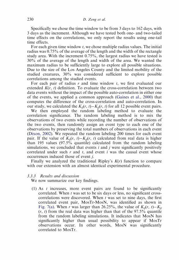
Specifically we chose the time window to be from 3 days to 162 days, with3 days as the increment. Although we have tested both one- and two-tailedtime effects on the correlations, we only report the results using one-tailtime effects.For each given time window t, we chose multiple radius values. The initial
radius was 0.75% of the average of the length and the width of the rectanglestudy area. With the increment 0.75%, the largest radius we have tested is30% of the average of the length and width of the area. We wanted themaximum radius to be sufficiently large to explore all possible situations.Due to the size of the Los Angeles County and the limited mobility of thestudied creatures, 30% was considered sufficient to explore possiblecorrelations among the studied events.For each pair of radius r and time window t, we first evaluated our
extended K(r, t) definition. To evaluate the cross-correlation between twodata events without the impact of the possible auto-correlation in either oneof the events, we applied a common approach (Gaines et al., 2000) thatcomputes the difference of the cross-correlation and auto-correlation. Inour study, we calculated the Kij(r, t)�Kjj(r, t) for all 12 possible event pairs.We then employed the random labeling method to evaluate the
correlation significance. The random labeling method is to mix theobservations of two events while recording the number of observations ofthe two events, then randomly assign an event type to each one of theobservations by preserving the total numbers of observations in each event(Dixon, 2002). We repeated the random labeling 200 times for each eventpair. If the value of Kij(r, t)�Kjj(r, t) calculated from real data is higherthan 195 values (97.5% quantile) calculated from the random labelingsimulations, we concluded that events i and j were significantly positivelycorrelated under such r and t, and event i was the causal event whoseoccurrences induced those of event j.Finally we analyzed the traditional Ripley’s K(r) function to compare
with our extension with an almost identical experimental procedure.
3.3.3 Results and discussionWe now summarize our key findings.
(1) As t increases, more event pairs are found to be significantlycorrelated. When t was set to be six days or less, no significant cross-correlations were discovered. When t was set to nine days, the firstcorrelated event pair, MosTr-MosN, was identified as shown inFig. 7(a). When r was larger than 26.25%, the value of Kij(r, t)�Kjj
(r, t) from the real data was higher than that of the 97.5% quantilefrom the random labeling simulations. It indicates that MosN hassignificantly higher than usual possibility to appear if MosTrobservations occur. In other words, MosN was significantlycorrelated to MosTr.
D. Zeng et al.230
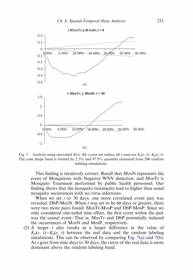
This finding is intuitively correct. Recall that MosN represents theevent of Mosquitoes with Negative WNV detection, and MosTr isMosquito Treatment performed by public health personnel. Ourfinding shows that the mosquito treatments lead to higher than usualmosquito occurrences with no virus infections.When we set t to 30 days, one more correlated event pair was
revealed: DbP-MosN. When t was set to be 60 days or greater, therewere two more pairs found: MosTr-MosP and DbP-MosP. Since weonly considered one-tailed time effect, the first event within the pairwas the causal event. That is, MosTr and DbP potentially inducedthe occurrences of MosN and MosP, respectively.
(2) A larger t also results in a larger difference in the value ofKij(r, t)�Kjj(r, t) between the real data and the random labelingsimulations. This can be observed by comparing Fig. 7(a) and 7(b).As t goes from nine days to 30 days, the curve of the real data is moredominant above the random labeling band.
i: M osTr; j: M osN; t = 9
-0.5
-0.4
-0.3
-0.2
-0.1
0
0.1
0.2
0.00% 5.00% 10.00% 15.00% 20.00% 25.00% 30.00%
(a)
i: MosTr; j: MosN; t = 30
-1
-0.5
0
0.5
1
1.5
0.00% 5.00% 10.00% 15.00% 20.00% 25.00% 30.00%
(b)
Fig. 7. Analysis using one-tailed K(r). All x-axes are radius; all y-axes are Kij(r, t)�Kjj(r, t).
The cone shape band is formed by 2.5% and 97.5% quantiles estimated from 200 random
labeling simulations.
Ch. 8. Spatial-Temporal Data Analysis 231
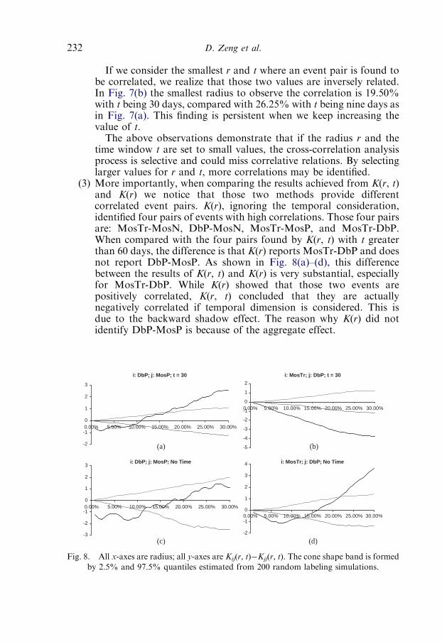
If we consider the smallest r and t where an event pair is found tobe correlated, we realize that those two values are inversely related.In Fig. 7(b) the smallest radius to observe the correlation is 19.50%with t being 30 days, compared with 26.25% with t being nine days asin Fig. 7(a). This finding is persistent when we keep increasing thevalue of t.The above observations demonstrate that if the radius r and the
time window t are set to small values, the cross-correlation analysisprocess is selective and could miss correlative relations. By selectinglarger values for r and t, more correlations may be identified.
(3) More importantly, when comparing the results achieved from K(r, t)and K(r) we notice that those two methods provide differentcorrelated event pairs. K(r), ignoring the temporal consideration,identified four pairs of events with high correlations. Those four pairsare: MosTr-MosN, DbP-MosN, MosTr-MosP, and MosTr-DbP.When compared with the four pairs found by K(r, t) with t greaterthan 60 days, the difference is that K(r) reports MosTr-DbP and doesnot report DbP-MosP. As shown in Fig. 8(a)–(d), this differencebetween the results of K(r, t) and K(r) is very substantial, especiallyfor MosTr-DbP. While K(r) showed that those two events arepositively correlated, K(r, t) concluded that they are actuallynegatively correlated if temporal dimension is considered. This isdue to the backward shadow effect. The reason why K(r) did notidentify DbP-MosP is because of the aggregate effect.
i: DbP; j: MosP; t = 30
-2
-1
0
1
2
3
0.00% 5.00% 10.00% 15.00% 20.00% 25.00% 30.00%
(a)
i: MosTr; j: DbP; t = 30
-5
-4
-3
-2
-1
0
1
2
0.00%
(b)
i: DbP; j: MosP; No Time
-3
-2
-1
0
1
2
3
0.00% 5.00% 10.00% 15.00% 20.00% 25.00% 30.00%
(c)
i: MosTr; j: DbP; No Time
-2
-1
0
1
2
3
4
(d)
5.00% 10.00% 15.00% 20.00% 25.00% 30.00%
0.00% 5.00% 10.00% 15.00% 20.00% 25.00% 30.00%
Fig. 8. All x-axes are radius; all y-axes are Kij(r, t)�Kjj(r, t). The cone shape band is formed
by 2.5% and 97.5% quantiles estimated from 200 random labeling simulations.
D. Zeng et al.232

In general, the traditional K(r) function tends to process data in anaggregated manner and sometimes fails to reveal meaningful correlations.Our extended measure reduces the aggregate effect and can eliminate thebackward shadow effect as well. Through adjusting an additional timewinder parameter, the domain experts have at their disposal a morebalanced and flexible analysis framework.
4 Conclusions
In this chapter, we have discussed two types of spatial-temporal dataanalysis techniques: clustering and correlation analysis. These techniqueshave wide applications in public health, natural sciences, as well as businessapplications.In the area of spatial-temporal clustering analysis, this chapter introduces
both retrospective and prospective hotspot analysis methods. Comparedwith retrospective methods, prospective analysis methods provide a morepowerful data analysis framework. Prospective methods are aimed atidentifying spatial-temporal interaction patterns in an online context anddo not require preprocessing data points into the baseline and cases ofinterest. We have provided a survey of major types of retrospective andprospective analysis techniques and presented a case study in public healthsurveillance to demonstrate the potential value of these techniques in real-world security informatics applications.As for spatial-temporal correlation analysis, we discuss both spatial
correlation measures as well as their spatial-temporal variations. Wedemonstrate various problems associated with purely spatial techniquesand advocate the development of measures that consider both spatial andtemporal coordinates in an integrated manner. One such attempt, extendingthe Ripley’s K(r) function, is shown to be more discriminating and providesthe ability to identify the causal events whose occurrences induce those ofother events.In the business computing arena, as technologies such as RFID and
Geospatial mash-ups as part of Web 2.0 are making their way to businesspractice and web-based product and service offerings, we believe thatbusiness applications of spatial-temporal data analysis techniques, someof the prominent ones surveyed in this chapter, will experience explosivegrowth. From a research perspective, such applications may provide fruitfulgrounds for technical innovations. We conclude this chapter by pointingout two significant opportunities in this emerging wave of research. First,as business applications typically involve large quantities of transactionaldata generated on a real-time basis, developing scalable spatial-temporaldata analysis techniques, possibly at the expense of reduced accuracyand sensitivity, is critical. This is particularly true in correlation research,as most existing studies focus on measures and model interpretations.
Ch. 8. Spatial-Temporal Data Analysis 233

Second, the interface between spatial-temporal data analysis and businessdecision-making holds opportunities which can lead to major findings withpractical relevance. Yet, research in this area is just starting. How to findmeaningful ways of leveraging the results of spatial-temporal data analysisin decision making contexts could well become an emerging ‘‘hotspot’’ inthe research landscape.
Acknowledgments
We would like to thank the members of the NSF BioPortal team forinsightful discussions. Various BioPortal public health partners haveprovided datasets which were used in the research reported in this chapter.We also would like to acknowledge funding support provided by the U.S.National Science Foundation through Grant IIS-0428241. The first authorwishes to acknowledge support from the National Natural ScienceFoundation of China (60621001, 60573078), the Chinese Academy ofSciences (2F07C01, 2F05N01), and the Ministry of Science and Technology(2006CB705500, 2006AA010106).
References
Ben-Hur, A., D. Horn, H.T. Siegelmann, V. Vapnik (2001). Support vector clustering. Journal of
Machine Learning Research 2, 125–137.
Cappaert, D.L., F.A. Drummond, P.A. Logan (1991). Population-dynamics of the Colorado potato
beetle (coleoptera, chrysomelidae) on a native host in Mexico. Environmental Entomology
20(December), 1549–1555.
Chang, W., D. Zeng, H. Chen (2005). A novel spatio-temporal data analysis approach based on
prospective support vector clustering, in: Workshop on Information Technologies and Systems,
Las Vegas, Nevada.
Chang, W., D. Zeng, H. Chen (2008). A stack-based prospective spatio-temporal data analysis
approach. Decision Support Systems 45, 697–713.
Diggle, P.J., A.G. Chetwynd (1991). Second-order analysis of spatial clustering for inhomogeneous
populations. Biometrics 47(September), 1155–1163.
Diggle, P.J., J. Besag, J.T. Gleaves (1976). Statistical-analysis of spatial point patterns by means of
distance methods. Biometrics 32, 659–667.
Dixon, P.M. (2002). Ripley’s K function, in: Encyclopedia of Environmetrics, Vol. 3. Wiley, Chichester,
pp. 1796–1803.
Gaines, K.F., A.L. Bryan, P.M. Dixon (2000). The effects of drought on foraging habitat selection of
breeding wood storks in coastal Georgia. Waterbirds 23, 64–73.
Halkidi, M., Y. Batistakis, M. Vazirgiannis (2002a). Cluster validity methods: Part 1. SIGMOD Record
31, 40–45.
Halkidi, M., Y. Batistakis, M. Vazirgiannis (2002b). Clustering validity checking methods: Part II.
SIGMOD Record 31, 19–27.
Johnson, S.C. (1967). Hierarchical clustering schemes. Psychometrika 2, 241–254.
Kulldorff, M. (1997). A spatial scan statistic. Communications in statistics—Theory and methods 26,
1481–1496.
D. Zeng et al.234

Kulldorff, M. (2001). Prospective time periodic geographical disease surveillance using a scan statistic.
Journal of the Royal Statistical Society A 164, 61–72.
Lean, I.J., T.B. Farver, H.F. Troutt, M.L. Bruss, J.C. Galland, R.L. Baldwin, C.A. Holmberg, L.D.
Weaver (1992). Time-series cross-correlation analysis of postparturient relationships among serum
metabolites and yield variables in Holstein cows. Journal of Dairy Science 75(July), 1891–1900.
Levine, N. (2002). CrimeStat III: A spatial statistics program for the analysis of crime incident locations.
The National Institute of Justice, Washington, DC.
Moran, P.A.P. (1948). The interpretation of statistical maps. Journal of the Royal Statistical Society
Series B—Statistical Methodology 10, 243–251.
Peterson, C.J., E.R. Squiers (1995). An unexpected change in spatial pattern across 10 years in an aspen
white-pine forest. Journal of Ecology 83(October), 847–855.
Procknor, M., S. Dachir, R.E. Owens, D.E. Little, P.G. Harms (1986). Temporal relationship of the
pulsatile fluctuation of luteinizing-hormone and progesterone in cattle—A time-series cross-
correlation analysis. Journal of Animal Science 62(January), 191–198.
Ripley, B.D. (1976). Second-order analysis of stationary point processes. Journal of Applied Probability
13, 255–266.
Ripley, B.D. (1981). Spatial Statistics. Wiley, New York.
Rogerson, P.A. (1997). Surveillance systems for monitoring the development of spatial patterns.
Statistics in Medicine 16, 2081–2093.
Rogerson, P.A. (2001). Monitoring point patterns for the development of space–time clusters. Journal of
the Royal Statistical Society A 164, 87–96.
Sonesson, C., D. Bock (2003). A review and discussion of prospective statistical surveillance in public
health. Journal of the Royal Statistical Society: Series A 166, 5–12.
Stoyan, D., A. Penttinen (2000). Recent applications of point process methods in forestry statistics.
Statistical Science 15(February), 61–78.
Thioulouse, J., D. Chessel, S. Champely (1995). Multivariate analysis of spatial patterns: A unified
approach to local and global structures. Environmental and Ecological Statistics 2, 1–14.
Tichy, J. (1973). Application of correlation and fourier-transform techniques in architectural and
building acoustics. Journal of the Acoustical Society of America 53, p. 319.
Veit, I. (1976). Application of correlation technique in acoustics and vibration engineering. Acustica 35,
219–231.
Waldhor, T. (1996). The spatial autocorrelation coefficient Moran’s I under heteroscedasticity. Statistics
in Medicine 15(April 15), 887–892.
Yao X. (2003). Research issues in spatio-temporal data mining, in: UCGIS workshop on Geospatial
Visualization and Knowldge Discovery, Lansdowne, VA.
Zeng, D., W. Chang, H. Chen (2004). A comparative study of spatio-temporal hotspot analysis
techniques in security informatics, in: Proceedings of the 7th IEEE International Conference on
Intelligent Transportation Systems, Washington.
Zeng, D., W. Chang, H. Chen (2005). Clustering-based spatio-temporal hotspot analysis techniques in
security informatics. IEEE Transactions on Intelligent Transportation Systems.
Ch. 8. Spatial-Temporal Data Analysis 235

This page intentionally left blank
Adomavicius & Gupta, Eds., Handbooks in Information Systems, Vol. 3
Copyright r 2009 by Emerald Group Publishing Limited
Chapter 9
Studying Heterogeneity of Price Evolutionin eBay Auctions via Functional Clustering
Wolfgang Jank and Galit ShmueliDepartment of Decisions, Operations and Information Technologies and the Center for Electronic
Markets and Enterprises, The Robert H. Smith School of Business, University of Maryland,
College Park, MD 20742, USA
Abstract
Electronic commerce, and in particular online auctions, have received anextreme surge of popularity in recent years. While auction theory has beenstudied for a long time from a game theory perspective, the electronicimplementation of the auction mechanism poses new and challenging researchquestions. In this work, we focus on the price formation process and itsdynamics. We present a new source of rich auction data and introduce aninnovative way of modeling and analyzing price dynamics. Specifically, thegoal of this chapter is to characterize heterogeneity in the price formationprocess and understand its sources. We represent the price process in auctionsas functional objects by accommodating the special structure of bidding data.We then use curve clustering to segment auctions and characterize each cluster,and then directly model cluster-specific price dynamics via differentialequations. Our findings suggest that there are several types of dynamics evenfor auctions of comparable items. Moreover, by coupling the dynamics withinformation on the auction format, the seller and the winner, we find newrelationships between price dynamics and the auction environment, and we tiethese findings to the existing literature on online auctions. Our results also showa significant gain in information compared to a traditional clustering approach.
1 Introduction
The public nature of many online marketplaces has allowed empiricalresearchers new opportunities to gather and analyze data. One example of anonline marketplace is the online auction. Online auctions have become apopular way for both businesses and consumers to exchange goods. One of
237
the biggest online marketplaces, and currently the biggest Consumer-to-Consumer (C2C) online auction place, is eBay (www.ebay.com).In 2005, eBay had 180.6 million registered users, of which over 71.8 millionbid, bought, or listed an item during the year. The number of listings in 2005was 1.9 billion, amounting to $44.3 billion in gross merchandize volume.1 Atany point in time there are millions of items listed for sale, across thousandsof product categories. Since eBay archives detailed records of its completedauctions, it is a great source for immense amounts of high-quality data.There has been extensive research on classical auction theory (Klemperer,
1999; Milgrom and Weber, 1982). Classical auction theory typically focuseson the analysis of optimal auctions and the effects of relaxing some of theirassumptions. While there has been some empirical research in the area(Hendricks and Paarsch, 1995), more and more bidding data are nowbecoming accessible thanks to the recent surge of online auctions and thecapability of collecting data conveniently over the Internet. While onlineauctions have the advantage of increasing the understanding of classicalauction theory, they also pose new research questions. Recent researchsuggests the need for additional investigation of the impact of the electronicimplementation on the auction mechanism (Klein and O’Keefe, 1999).In fact, empirical studies provide evidence that classical auction theory maynot generally carry over to the online context (Lucking-Reiley, 1999).Reasons such as the anonymity of the Internet, its worldwide reach free ofgeographical boundaries and time, and the longer duration of onlineauctions, can contribute to deviation from what classical auction theorypredicts. One example is the observed phenomenon of ‘‘bid sniping’’, wherea large volume of bids arrives in the final moments of the auction (Roth andOckenfels, 2002). According to auction theory, this bidding strategy is notoptimal for the bidder in a second-price auction like eBay, and is also nottypically observed in offline auctions (Pinker et al., 2003).Empirical research of online auctions has been growing fast in the last few
years. Studies use data from online auction houses such as eBay, Yahoo!and uBid but eBay’s market dominance and its data accessibility have madeit by far the center of research efforts (Ba and Pavlou, 2002; Bajari andHortacsu, 2003; Bapna et al., 2004, 2008; Dellarocas, 2003; Hyde et al.,2006; Klein and O’Keefe, 1999; Lucking-Reiley, 1999, 2000; Roth andOckenfels, 2002; Shmueli and Jank, 2005; Wang et al., 2008). Most of thesestudies rely on large databases that are collected using ‘‘web spiders’’, whichare software programs that are designed to ‘‘crawl’’ over webpages andcollect designated data into a database.In this work we consider a feature of online auctions that has been mostly
overlooked in the auction literature: The price process and its dynamicsduring an auction. Rather than characterizing an auction solely by its
1See eBay’s press release from 1/18/2006 available at investor.ebay.com/releases.cfm?Year ¼ 2006
W. Jank and G. Shmueli238

‘‘static’’ outcome such as the final price or the number of bids, wecharacterize it by its dynamic price formation process throughout theauction. The goal of this chapter is to better understand the heterogeneityof price dynamics in different auctions, by segmenting auctions into clustersaccording to their price processes, and then characterizing the dynamicsof each cluster. To do so, we first estimate price curves from bid historiesand quantify their dynamics by calculating curve derivatives. We thensearch for ‘‘types’’ or ‘‘profiles’’ of auctions that have similar dynamics, andsupplement these profiles with static auction information to obtain acomprehensive descriptions of auction types. We further study each clusterby directly modeling price dynamics through differential equations. Finally,static information about the auction is integrated into the dynamic systemin order to shed light on their combined behavior.The ability to describe price dynamics in an online auction or to classify
an auction into certain dynamic types can be useful for the seller, thebidder, and the auction house. Some examples are realtime forecasting ofthe final price while the auction is still ongoing (Wang et al., 2008); selectingwhich auction to bid on among a set of competing auctions; selectingauction settings (by the seller) that are associated with fast price dynamics;pricing auction options (by the auction house) that guarantee faster priceincreases; and detecting suspicious price dynamics that may suggestfraudulent bidding activity.We address these tasks using functional data analysis (FDA). In FDA,
the object of interest is a set of curves, shapes, objects, or, more generally,a set of functional observations (Ramsay and Silverman, 2002, 2005). In theauction context, we represent the auction price process as a functionalobject. That is, we interpret the process of price changes between the startand the end of the auction as a continuous curve. We refer to this process asthe auction’s price evolution. In that sense, every auction is associated witha functional object describing the price between its start and end. Severalmillion auctions transact on eBay every day. We segment auctions intogroups with more homogeneous price evolutions to learn about pricepatterns. We do so by using curve clustering (Abraham et al., 2003; Jamesand Sugar, 2003; Tarpey and Kinateder, 2003). Our results show that curveclustering can lead to new insights about the auction process compared totraditional (non-functional) approaches.The chapter is organized as follows. In Section 2 we describe online
auction data and the mechanism that generates and collects them. InSection 3 we discuss the functional representation of price via a smoothcurve and quantify price dynamics via curve derivatives. Section 4 usescurve clustering to segment online auctions according to their pricepatterns. We investigate the details of each cluster and estimate differentialequations which capture the differences in price formation in a compact(and novel) way. We use a data set of Palm Pilot eBay auctions throughoutthe chapter. The chapter concludes with final remarks in Section 5.
Ch. 9. Studying Heterogeneity of Price Evolution in eBay Auctions 239

2 Auction structure and data on eBay.com
Since eBay is by far the largest source of data and empirical work in thisfield, we focus here on its format and data structure. However, ourfunctional approach can be readily adapted to different data originatingfrom other types of auctions.
2.1 How eBay auctions work
The dominant auction format on eBay is a variant of the second pricesealed-bid auction (Krishna, 2002) with ‘‘proxy bidding’’. This means thatindividuals submit a ‘‘proxy bid’’, which is the maximum value they arewilling to pay for the item. The auction mechanism automates the biddingprocess to ensure that the person with the highest proxy bid is in the lead ofthe auction. The winner is the highest bidder and pays the second highestbid. For example, suppose that bidder A is the first bidder to submit aproxy bid on an item with a minimum bid of $10 and a minimum bidincrement of $0.50. Suppose that bidder A places a proxy bid of $25. TheneBay automatically displays A as the highest bidder, with a bid of $10.Next, suppose that bidder B enters the auction with a proxy bid of $13.eBay still displays A as the highest bidder; however it raises the displayedhigh-bid to $13.50, one bid increment above the second highest bid. Ifanother bidder submits a proxy bid above $25.50, bidder A is no longer inthe lead. However, if bidder A wishes, he or she can submit a new proxybid. This process continues until the auction ends. Unlike other auctions,eBay has strict ending times, ranging between 1 and 10 days from theopening of the auction, as determined by the seller. eBay posts the completebid histories of closed auctions for a duration of at least 30 days on itswebsite.2
2.2 eBay’s data
Figure 1 shows an example of a bid history found on eBay’s website. Thetop of Fig. 1 displays a summary of the auction: The item for sale, the currentbid, the starting bid, the number of bids received, the start and end times,and the seller’s username together with his/her rating (in parentheses). Thebottom of the page includes detailed information on the history of bids.Starting with the highest bid, the bottom displays the bidder’s user name, therating and the time and date when the bid was placed.The data for this study are the complete bid histories from 183 closed
auctions for new Palm M515 Personal Digital Assistant (PDA) units on
2See http://listings.ebay.com/pool1/listings/list/completed.html
W. Jank and G. Shmueli240

eBay.com. These data are available at www.smith.umd.edu/ceme/statistics/.We chose the Palm M515 since it was a very popular item on eBay atthe time, with a multitude of different auctions every day. All of theauctions were 7 days long and took place from mid-March through
home | register | sign in | services | site map | help
tips
Search titles and descriptions
eBay.com Bid History for PALM M515 COLOR PDA LIKE NEW HANDHELD (Item # 3041545039)
Currently $157.50 First bid $60.00Quantity 1 # of bids 19Time left Auction has ended. Started Aug-16-03 10:34:26 PDTEnds Aug-21-03 10:34:26 PDT
Seller (Rating) daynathegreat ( 27 )
(Accessible by Seller only) Learn more.
Bidding History (Highest bids first)
Date of BidBid AmountUser ID
moonwolfdesigns ( 481 ) $157.50 Aug-21-03 10:33:20 PDT
rondaroo1 ( 65 ) $155.00 Aug-21-03 10:32:52 PDT
moonwolfdesigns ( 481 ) $151.99 Aug-21-03 10:19:00 PDT
rondaroo1 ( 65 ) $150.00 Aug-21-03 10:32:23 PDT
rondaroo1 ( 65 ) $145.00 Aug-21-03 10:32:11 PDT
rondaroo1 ( 65 ) $140.00 Aug-21-03 09:01:49 PDT
cpumpkinbatman ( 16 ) $125.95 Aug-21-03 10:03:09 PDT
cpumpkinbatman ( 16 ) $120.95 Aug-21-03 10:02:45 PDT
moonwolfdesigns ( 481 ) $115.95 Aug-21-03 08:31:09 PDT
quest3487 ( 68 ) $110.25 Aug-21-03 07:48:01 PDT
moonwolfdesigns ( 481 ) $108.35 Aug-21-03 08:28:58 PDT
moonwolfdesigns ( 481 ) $102.75 Aug-21-03 07:25:57 PDT
quest3487 ( 68 ) $100.25 Aug-21-03 07:19:48 PDT
moonwolfdesigns ( 481 ) $100.00 Aug-21-03 07:25:43 PDT
moonwolfdesigns ( 481 ) $95.00 Aug-21-03 07:25:30 PDT
moonwolfdesigns ( 481 ) $90.00 Aug-21-03 07:25:11 PDT
Search
Fig. 1. Partial bid history for an eBay auction. The top includes summary information on the
auction format, the seller and the item sold; the bottom includes the detailed history of the
bidding. Notice that the bids are ordered by descending bid amounts, not chronologically.
Since the current highest bid is not revealed, later bids can be lower than earlier ones.
Ch. 9. Studying Heterogeneity of Price Evolution in eBay Auctions 241
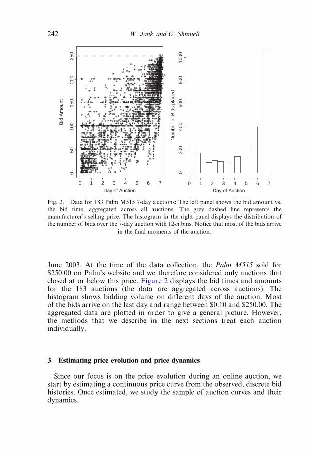
June 2003. At the time of the data collection, the Palm M515 sold for$250.00 on Palm’s website and we therefore considered only auctions thatclosed at or below this price. Figure 2 displays the bid times and amountsfor the 183 auctions (the data are aggregated across auctions). Thehistogram shows bidding volume on different days of the auction. Mostof the bids arrive on the last day and range between $0.10 and $250.00. Theaggregated data are plotted in order to give a general picture. However,the methods that we describe in the next sections treat each auctionindividually.
3 Estimating price evolution and price dynamics
Since our focus is on the price evolution during an online auction, westart by estimating a continuous price curve from the observed, discrete bidhistories. Once estimated, we study the sample of auction curves and theirdynamics.
*
*
***** *
*
*
*
***
*
*
**
** ***
**
*****
*
****
*
*
**
** **
* ****
****
*
*
****************
*
*
*
*
*
*
*
*** **
*
*
*****
****
**
*
*
***************
** *
******
*******
*
****
*
*
*
***
**
*
***
* * *
*
*
* ***** **
***** **
**
*
*
*******
*
****
*
*
*
*
*
*
*** *
*
****
** *
*
**
*
*
********* *
*
***
*
***
*******
***
***
*
*
**
*
* *
* *
*
*
*
*
*
**
*
*
** *
****** **
*
*******
**
*** *
******** *
*
* ***
***********
*
*****
** *
*
*
**
*****
*
*
*
*
*
*
****
**
*
******
**
*
*
*
* ******
*
*
*
*****
*
**
*
***
*
******** **** *
*
*
*
**
*
*
* ******
***
*
**
*
*
**
****
*
*
*
*
*
*
*
*
***
* *
**
**
* ****
******
*
*
****
*****
***
*
*******
*
** **
*
***
**
* ***
*
*
*
******
**
*
*****
*
*
**** *
****
* *
*
***
*
* ***
**
***
*
* *
*****
*
*
*******
***
*
**
***
***
**
*
*****
*
*
* **
** *
** *
*
***
*
*
*
***** *
*
*
****
* *** *
**
*
*****
*
*
**
**********
*
*
**
***** * **
****
******
*
***
*
**
*
** **
*
**
***
**
***
*
** **
* * * **
*
*
**
*** *
*
****
****
* *
*
**
** **
* ******
*****
**
*
**
*
***
*
***
**
* *
*
*** ***
*
*
*
*
*
*
*
*
**
**
****
***
*
***
**
*
***
*
**
*
*
******** * *
**
* *****
*
******* *
****
*
***
***
*
*
*
*
*
**************
**
*
**
**
**
* **
*
*
* ***********
*********
*
****
* **
*
* **
****
*
****
*** *
***
***
*
*
** ****
*****
*
****
***
***
*****
*
* *
*
*
***
*
**** ****
****** **
** ***
**
** *
*
*
*
*
**
*
*
*
*
*****
*
**
*
***
*
******
*****
*
****
*
*
* ******
*
*
**
*
******
*
*
*
*
*
*
****** * *
*
**
* ***
*****
*
******
*
**
**
*
**
*
*** ***
***
**********
*
*
****
*
***
*** ****
*
*
***** **
*
*
**
*****
*
*
*
**
***
*** * *
*
***
*
**
*
****************
*****
** *
*
**
*
***
**
*
***
*
*
******
***
***
***
*
* *
*
**
*
*
**
******
* **
*
*
*
*
*
****
***** *
*
* *
*
******
*
*******
**
****
***** *
* * *
*
*
*
*
*
**
****************
*
*
** * ***
******
*****
*
*
***
*
*
*
*
*
******
*
*
***
******
***
*
*
** * ****
*
**
*
**
*
*
*****
*
* **
*
**
*
**
****** **
**
**
*
***
**
*
*
* *
*
*
**
*
*
*
*****
********
*
*
*
*
*
*
*
***
**
****
*
***
**
*
*
*
*
*
***
***
*********
****
*
*****
*
******
***
***
** *
**
* *
*
*
*
****
**
*
*
**
*
*
*
****
*
*
*
*
*
*
** *
*
**
***********
*
*
*
* **
*
***********
*
*
****
***
*
***
**
*
*****
****
*
*
*
*
*
**
****
*
****
*
*
***
*
****
*
*
*
**********
*
***
*****
********
** ***
*
*
***
**
*
**
***
*
********
* *
**
* **** * *
*
*****
*
**
*
*
** ** *
******
****
*
***
*
*
* ***
**
****
*
*
**
*
****
**
***
*****
******
*
*
**
*
**
**
***
***
******
*
****
*****
*
*
****
**************
*
****** **
******
**
*
*
*****
*** **
*
***
*****
*****
*
******
* *
*** *
** ****
******
*
*
**
*
*******
*
*
** *
**
*
*
*
*
**
*
**
**
*
*****
****
*****
* ** *******
*
*
*
*
*
* * ***
**
* ***
*
*
* *
*********
*
* *
** * ***
*
**
*
*
*******
** **
****
*
*
*****
*****
*
*******
*
*
*
*
**
**** ***
******
*
**
** *
*
***
****
*****
****
*
* **
*
*
************
***
***
*
*
***
**
*
*
*
****
*
************
****
**
**
*
**
*
**
*
***
**
*****
*
*
****
**
*
**
****
*
***
***
*
**** **
*
*********
*
*
*
**
*
**
*****
*
********
****
*
*
*
*
*
**
*
***
** *
*
*
*
**
*
*
*
***
*** *
*****
***
**
*
**
*
* ***
*
* ********
*
*
****
**
*
*
**
******
*
****
****
**********
***
*
*
******
*
*
*
****
*
*****
* *
*
**
*****
*
*
**
**
*
**
*
*
* **** *****
**
*****
*
********
***
**
***
* * *
** *
* *****************
*
**********
*******
*
*
****
******
**
*
*
**
*
*
*
** *
****
***
****
**
*
* ** * ***
**
*
****
**
*
******
*
****
*
*
*
*
******
**
***
****
*
*
*
*
*
*
*** *
****
***
*
*
**
**
*****
*
*
*
**
*
*** ***
*****
*
*
*
*
****
***
******
* **
*
******
*
**
** *******
* ** * ** *
*
******
*
***
*
**
******
***********
**
*
*
*
* *
** **** * *
*****
*
*
*
**
* * ******
*
*** *
*
***
**
*
******
*
***
****
*
*
*
***** ***
**
**
****
*
******
**
*
*
*
*
*******
**
***
* * **
**
***
*** *
** **
*
***
**
*
*
*
**
****
*
*******
**
*
***** **
*
*********
*
****
*
*
***
*
***
* * *
*
*******
*
***
*
*
****
****
****
**
*
*
* ** ** *
*****
*
*
***
******
*
**
* **
*
***
*
***
* *****
***
********
** * **
*****
*
******* **
**
*****
*
****
**
****
*
*** *
*
* *
*
****
*
*
*****
** * ** *
*
******* ***
**
********
*
****
*
** **
***
*****
**
*
** **
* *
*
**
***
**
*
*
*
* *****
**
*****
*******
*
**
**
*
*****
* ****
*******
**
*
*
*
***
*
*
***
*
***
* *
*
*
*
*** **
** *
*
*
***
*
*
* *
*
* *
**
*
*
*
*
**** *
** ***
****
* *
****
*
*
*
*
*
*
*
*
*
*
*****
*
***
*
**
*****
*
*
**** ** *
***
*************
*
***
**
*
*
*
***
******
*****
*****
*
*
*
*
*
**
*
*****
*
* *****
250
Day of Auction
Bid
Am
ount
Day of Auction
Num
ber
of B
ids
plac
ed
050
100
150
200
0 1 2 3 4 5 6 7 0 1 2 3 4 5 6 710
000
200
400
600
800
Fig. 2. Data for 183 Palm M515 7-day auctions: The left panel shows the bid amount vs.
the bid time, aggregated across all auctions. The grey dashed line represents the
manufacturer’s selling price. The histogram in the right panel displays the distribution of
the number of bids over the 7-day auction with 12-h bins. Notice that most of the bids arrive
in the final moments of the auction.
W. Jank and G. Shmueli242

3.1 Estimating a continuous price curve via smoothing
We start by estimating for each auction its underlying price curve. Toobtain the price curve, we first compute the ‘‘live bid’’ function, a stepfunction that reflects the price as it was seen on eBay during the ongoingauction.3 Figure 3 displays the live bid step function for two auctions in ourdata set.Since we assume a smooth underlying price curve, and because we are
interested in quantifying its dynamics, we use polynomial smoothing splines(Ramsay and Silverman, 2005; Ruppert et al., 2003) to transform the stepfunction into a smooth functional object which we denote by f(t). A varietyof different smoothers exist. One very flexible and computationally efficientchoice is the penalized smoothing spline. Let t1, . . . , tL be a set of knots.Then, a polynomial spline of order p is given by
f ðtÞ ¼ b0 þ b1tþ b2t2 þ � � � þ bpt
p þXLl¼1
bplðt� tlÞpþ (1)
7
300
Auction 3013787547
Day
Pric
e
7
300
Auction 3015682701
Day
Pric
e
0 1 2 3 4 5 6
050
100
150
200
250
050
100
150
200
250
0 1 2 3 4 5 6
Fig. 3. Live bids (circles) and associated step function reflecting price during the live
auction.
3Computing the live bid from the bid history is possible using eBay’s increment table. Seepages.ebay.com/help/basics/g-bid-increment.html
Ch. 9. Studying Heterogeneity of Price Evolution in eBay Auctions 243

where uþ ¼ uI ½u�0� denotes the positive part of the function u. Define theroughness penalty
PENmðtÞ ¼
ZfDmf ðtÞg2dt (2)
where Dmf, m ¼ 1, 2, 3, . . . , denotes the mth derivative of the function f.The penalized smoothing spline f minimizes the penalized squared error
PENSSl;m ¼
ZfyðtÞ � f ðtÞg2dtþ l PENmðtÞ (3)
where y(t) denotes the observed data at time t and the smoothing parameterl controls the tradeoff between data fit and smoothness of the function f.Using m ¼ 2 in Eq. (3) leads to the commonly encountered cubic smoothingspline. Other possible smoothers include the use of B-splines or radial basisfunctions (Ruppert et al., 2003).We use the same family of smoothers (i.e., the same spline order, the same
set of knots, and the same smoothing parameters) for all auctions so thatdifferent auctions differ only with respect to their spline coefficients. Ourchoices of spline order, smoothing parameter, and knots are closely tied toour goal and the nature of the data. In general, choosing a spline of order pguarantees that the first p� 2 derivatives are smooth (Ramsay andSilverman, 2002). Since we are interested in studying at least the first twoderivatives of the price curves, we use splines of order 5. Knot locations arechosen according to expected changepoints in the curves (a separatepolynomial is fit between each set of consecutive knots). In our case, theselection of knots is based on the empirical bidding frequencies, and inparticular accounts for the phenomenon of ‘‘sniping’’ or ‘‘last momentbidding’’ (Roth and Ockenfels, 2002; Shmueli et al., 2007). In order tocapture the increased bidding activity at the end, we place an increasingnumber of knots toward the auction end. Specifically, our selection of knotsmirrors the distribution of bid arrivals: We place 7 equally spaced knotsevery 24 h along the first 6 days of the auction, that is, tl ¼ 0, . . . , 6;l ¼ 1, . . . , 7. Then, over the first 18 h of the final day, we place knots overshorter intervals of 6 h each, that is, t8 ¼ 6.25, t9 ¼ 6.5, and t10 ¼ 6.75. Andfinally, we divide the last 6 h of the auction into 4 intervals of 1 1/2 h each,letting t11 ¼ 6.8125, t12 ¼ 6.8750, t13 ¼ 6.9375, and t14 ¼ 7.0000. Thechoice of the smoothing parameter l is based on visual inspection of thecurves with the goal of balancing data fit and smoothness.4 This leads us toa value of l ¼ 50.Finally, because of the high frequency of late bids (see Fig. 2), the
price can take significant jumps at the end of the auction (as in the right
4Generalized cross-validation (GCV) did not lead to visually very appealing representations of theprice evolution.
W. Jank and G. Shmueli244
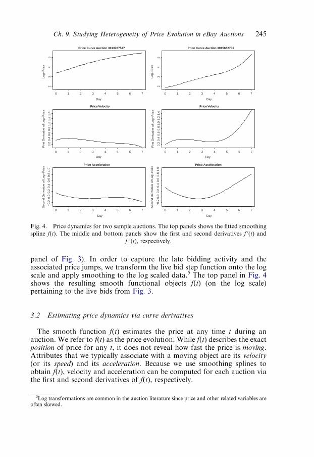
panel of Fig. 3). In order to capture the late bidding activity and theassociated price jumps, we transform the live bid step function onto the logscale and apply smoothing to the log scaled data.5 The top panel in Fig. 4shows the resulting smooth functional objects f(t) (on the log scale)pertaining to the live bids from Fig. 3.
3.2 Estimating price dynamics via curve derivatives
The smooth function f(t) estimates the price at any time t during anauction. We refer to f(t) as the price evolution. While f(t) describes the exactposition of price for any t, it does not reveal how fast the price is moving.Attributes that we typically associate with a moving object are its velocity(or its speed) and its acceleration. Because we use smoothing splines toobtain f(t), velocity and acceleration can be computed for each auction viathe first and second derivatives of f(t), respectively.
23
45
Price Curve Auction 3013787547
Day
Log−
Pric
e
23
45
Price Curve Auction 3015682701
Day
Log−
Pric
e
1.4
Price Velocity
Firs
t Der
ivat
ive
of L
og−
Pric
e
0.2
Price Velocity
Firs
t Der
ivat
ive
of L
og−
Pric
e
1.0
Price Acceleration
Day
Sec
ond
Der
ivat
ive
of L
og−
Pric
e
−0.
2
Price Acceleration
Day
Sec
ond
Der
ivat
ive
of L
og−
Pric
e
0 1 2 3 4 5 6 7
Day
0 1 2 3 4 5 6 7
0 1 2 3 4 5 6 7 0 1 2 3 4 5 6 7
Day
0 1 2 3 4 5 6 7
0 1 2 3 4 5 6 7
0.2
0.4
0.6
0.8
1.0
1.2
−0.
20.
00.
20.
40.
60.
8
1.4
1.2
1.0
0.8
0.6
0.4
1.0
0.8
0.6
0.4
0.2
0.0
Fig. 4. Price dynamics for two sample auctions. The top panels shows the fitted smoothing
spline f(t). The middle and bottom panels show the first and second derivatives f u(t) and
f v(t), respectively.
5Log transformations are common in the auction literature since price and other related variables areoften skewed.
Ch. 9. Studying Heterogeneity of Price Evolution in eBay Auctions 245
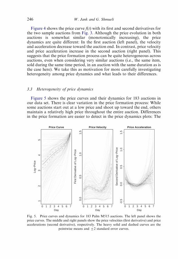
Figure 4 shows the price curve f(t) with its first and second derivatives forthe two sample auctions from Fig. 3. Although the price evolution in bothauctions is somewhat similar (monotonically increasing), the pricedynamics are quite different: In the first auction (left panel), the velocityand acceleration decrease toward the auction end. In contrast, price velocityand price acceleration increase in the second auction (right panel). Thissuggests that the price formation process can be quite heterogeneous acrossauctions, even when considering very similar auctions (i.e., the same item,sold during the same time period, in an auction with the same duration as isthe case here). We take this as motivation for more carefully investigatingheterogeneity among price dynamics and what leads to their differences.
3.3 Heterogeneity of price dynamics
Figure 5 shows the price curves and their dynamics for 183 auctions inour data set. There is clear variation in the price formation process: Whilesome auctions start out at a low price and shoot up toward the end, othersmaintain a relatively high price throughout the entire auction. Differencesin the price formation are easier to detect in the price dynamics plots: The
54
32
1
Price Curve
Day
Log−
Pric
e
0.0
0.5
1.0
1.5
-0.5
0.0
0.5
1.0
1.5
Price Velocity
Day
Firs
t Der
ivat
ive
of L
og−
Pric
e
Price Acceleration
Day
Sec
ond
Der
ivat
ive
of L
og−
Pric
e
0 1 2 3 4 5 6 7 0 1 2 3 4 5 6 7 0 1 2 3 4 5 6 7
Fig. 5. Price curves and dynamics for 183 Palm M515 auctions. The left panel shows the
price curves. The middle and right panels show the price velocities (first derivative) and price
accelerations (second derivative), respectively. The heavy solid and dashed curves are the
pointwise means and 72 standard error curves.
W. Jank and G. Shmueli246
first derivative of the price curve shows that, on average, price increasesquickly during the first part of the auction. The velocity then slows down,only to increase sharply again after day 5. A similar picture is seen forthe average price acceleration: It is high at the onset of the auction, thendrops below zero (‘‘deceleration’’) only to sharply increase again towardthe end.Although it is tempting to talk about ‘‘typical’’ dynamics for these data,
we notice that there is significant variation among the curves. For instance,not all auctions show increasing price acceleration toward the end. In fact,in some auctions the price decelerates and ends at large negativeacceleration. Similarly, in many auctions there is no increase in the pricevelocity during the first part of the auction. All this suggests that the priceformation process of similar auctioned items is not as homogeneous asexpected. In the following we use functional cluster analysis to segmentauctions into groups of more homogeneous price dynamics.
4 Auction segmentation via curve clustering
4.1 Clustering mechanism and number of clusters
As in ordinary cluster analysis, our goal is to segment the data intoclusters of observations that are more homogenous in order to betterunderstand the characteristics or factors that lead to heterogeneity in thedata. Since our data are curves, we use curve clustering to find segments ofmore homogeneous price profiles.Curve clustering can be done in several ways. One option is to sample
each curve on a finite grid and then cluster on the grid. However, this canlead to unstable estimates (Hastie et al., 1995). A different approach thathas been explored in the literature only recently (Abraham et al., 2003) is tocluster the set of curve coefficients rather than the functions themselves(James and Sugar, 2003). Let B ¼ {b1, . . . , bN} be the set coefficientspertaining to the N polynomial smoothing splines. Since each of the Ncurves is based on the same set of knots and the same smoothingparameters, heterogeneity across curves is captured by the heterogeneityacross the coefficients. Thus, rather than clustering the original curves, wecluster the set of coefficients B.We use the K-medoids algorithm (with a Manhattan distance) since it
is more robust to extreme values than K-means (Cuesta-Albertos et al.,1997). The K-medoids algorithm iteratively minimizes the within-clusterdissimilarity
WK ¼XKk¼1
Xj; j02Ik
Dðbj; bj0 Þ (4)
Ch. 9. Studying Heterogeneity of Price Evolution in eBay Auctions 247

where D(bj,bju) denotes the dissimilarity between coefficients j and ju, and Ikdenotes the set of indices pertaining to the elements of the kth cluster,k ¼ 1, . . . ,K (Hastie et al., 2001; Kaufman and Rousseeuw, 1987).We investigate different choices for K and use several different criteria to
determine the most plausible number of clusters. The first is the popularmethod of examining the reduction in within-cluster dissimilarity as afunction of the number of clusters. This is shown in Fig. 6 (left panel),where we see that the within-cluster dissimilarity reduces by about 2 whenmoving from one to two clusters and also when moving from two to threeclusters. However, the reduction is less than 0.5 for a larger number ofclusters. The danger with this approach is that it is prone to show kinkseven if there is no clustering in the data (Sugar and James, 2003; Tibshiraniet al., 2001). We therefore also use an alternative measure based on aninformation theoretic approach introduced by (Sugar and James, 2003).This non-parametric measure of within-cluster dispersion, dK, also calledthe ‘‘distortion’’, is the average Mahalanobis distance per dimensionbetween each observation and its closest cluster center. Rather than usingthe raw distortions, Sugar and James (2003) suggest to use the ‘‘Jump
2
0.5
Reduction in the within−cluster dissimilarity
Number of clusters K
W[K
−1]
−W
[K]
1.4
e−
08
Information Theoretic Criterion
Number of clusters K
J[K
]
2.0
1.0
1.5
0.0
e+00
2.0
e−09
4.0
e−09
6.0
e−09
8.0
e−09
1.0
e−08
1.2
e−08
4 6 8 10 2 4 6 8 10
Fig. 6. Choosing the number of clusters: The left plot shows the reduction in the within-
cluster dissimilarity as the number of clusters increases. K ¼ 2 and K ¼ 3 clusters lead to a
strong reduction. As K>3, this reduction diminishes. The right plot shows the jump plot of
the transformed distortions. The largest jump occurs at K ¼ 3 providing additional evidence
for 3 clusters in the data.
W. Jank and G. Shmueli248

statistic’’ defined as JK ¼ d�YK � d�YK�1, where Y ¼ dim/2 and dim denotesthe dimension of the data. A graph of JK vs. K is expected to peak at thenumber of clusters K that best describes the data. A jump plot for our datais shown in the right panel of Fig. 6. The largest jump occurs at K ¼ 3,providing additional evidence for 3 clusters in the data.6
4.2 Comparing price dynamics of auction clusters
After determining the number of clusters in the data, we investigate eachcluster individually in order to derive insight about the differences in theprice formation process in the different clusters. For our data we obtain 3distinct clusters of sizes 90, 47, and 46 auctions. We start by comparingdifferences across cluster dynamics, and then supplement the dynamiccharacterization with differences in static auction features such as openingprice, seller reputation, and winner experience.In order to compare the price dynamics across clusters we plot cluster-
specific price curves and their derivatives together with 95% confidenceinterval bounds (see Fig. 7). A comparison of the price curves (top row)reveals that auctions in cluster 1 and 2, on average, start out at a higherprice than those in cluster 3. Also, the average price curves in cluster 2 and 3increase more sharply at the auction end. Differences in price dynamics aremore visible in the price velocities (second row) and accelerations (thirdrow): Cluster 1 is marked by high acceleration at the auction start, followedby a long period of stalling/decreasing dynamics which extends almost tothe end of day 6. The price then speeds up again toward closing. Cluster 2,in contrast, experiences hardly any price dynamics during the first five days,but toward the auction end the price speeds up rapidly at an increasing rate.In fact the maximum acceleration is reached at closing. Since accelerationprecedes velocity, a maximum acceleration at closing does not translate intomaximum speed. In other words, auctions in cluster 2 close before theyreach maximum speed. The picture for cluster 3 is different: Like cluster 1,it experiences some early dynamics, albeit of larger magnitude. Like cluster2, the dynamics slow down during mid-auction with a speeding up towardthe auction end. However, while auction prices in cluster 2 do not reachtheir maximum speed before closing, the ones in cluster 3 do! Notice thatacceleration in cluster 3 reaches its maximum a day before the auction endand then levels off. This means that the price velocity in cluster 3 is ‘‘maxedout’’ when the auction finishes. We further investigate the potential impactof these different price dynamics below, by directly modeling the pricedynamics.
6We also clustered a lower dimensional representation of the spline coefficients using principalcomponents and obtained similar results. Further evidence for 3 clusters was also obtained byperforming functional principal component analysis (Ramsay and Silverman, 2005).
Ch. 9. Studying Heterogeneity of Price Evolution in eBay Auctions 249
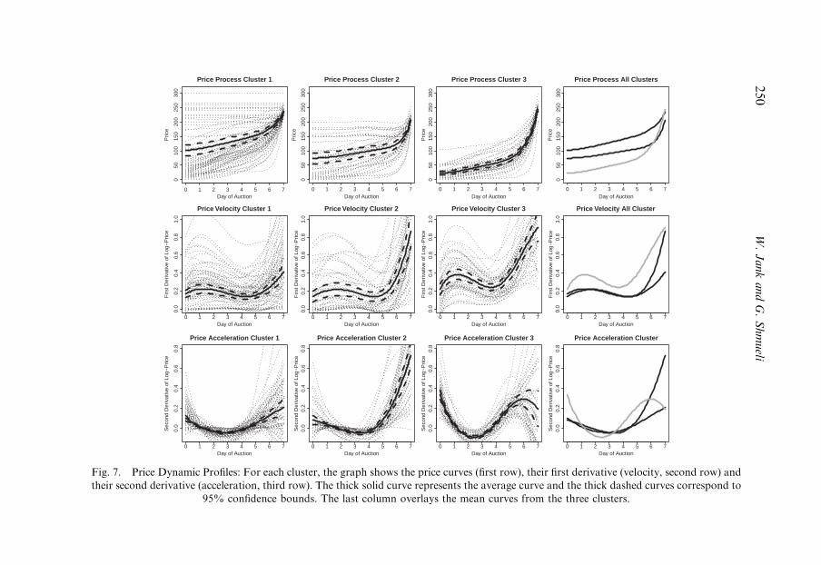
0 1 2 3 4 5 6 7
050
100
150
200
250
300
Price Process Cluster 1
Day of Auction
Pric
e
0 1 2 3 4 5 6 7
050
100
150
200
250
300
Price Process Cluster 2
Day of Auction
Pric
e
0 1 2 3 4 5 6 7
050
100
150
200
250
300
Price Process Cluster 3
Day of Auction
Pric
e
0 1 2 3 4 5 6 7
050
100
150
200
250
300
Price Process All Clusters
Day of Auction
Pric
e
0 1 2 3 4 5 6 7
0.0
0.2
0.4
0.6
0.8
1.0
Price Velocity Cluster 1
Day of Auction
Firs
t Der
ivat
ive
of L
og−
Pric
e
0 1 2 3 4 5 6 7
0.0
0.2
0.4
0.6
0.8
1.0
Price Velocity Cluster 2
Day of Auction
Firs
t Der
ivat
ive
of L
og−
Pric
e
0 1 2 3 4 5 6 7
0.0
0.2
0.4
0.6
0.8
1.0
Price Velocity Cluster 3
Day of Auction
Firs
t Der
ivat
ive
of L
og−
Pric
e
0 1 2 3 4 5 6 7
0.0
0.2
0.4
0.6
0.8
1.0
Price Velocity All Cluster
Day of Auction
Firs
t Der
ivat
ive
of L
og−
Pric
e
0 1 2 3 4 5 6 7
0.0
0.2
0.4
0.6
0.8
Price Acceleration Cluster 1
Day of Auction
Sec
ond
Der
ivat
ive
of L
og−
Pric
e
0 1 2 3 4 5 6 7
0.0
0.2
0.4
0.6
0.8
Price Acceleration Cluster 2
Day of Auction
Sec
ond
Der
ivat
ive
of L
og−
Pric
e
0 1 2 3 4 5 6 7
0.0
0.2
0.4
0.6
0.8
Price Acceleration Cluster 3
Day of Auction
Sec
ond
Der
ivat
ive
of L
og−
Pric
e
0 1 2 3 4 5 6 7
0.0
0.2
0.4
0.6
0.8
Price Acceleration Cluster
Day of Auction
Sec
ond
Der
ivat
ive
of L
og−
Pric
e
Fig. 7. Price Dynamic Profiles: For each cluster, the graph shows the price curves (first row), their first derivative (velocity, second row) and
their second derivative (acceleration, third row). The thick solid curve represents the average curve and the thick dashed curves correspond to
95% confidence bounds. The last column overlays the mean curves from the three clusters.
W.JankandG.Shmueli
250

4.3 A differential equation for price
The price curve and its derivatives appear to play an important role inunderstanding the price formation process in an auction. For this reason,we set out to model the relationship directly via functional differentialequation analysis. Consider a second-order homogenous linear differentialequation of the form
b0ðtÞf ðtÞ þ b1ðtÞf0ðtÞ þ f 00ðtÞ ¼ 0 (5)
This is a plausible model for describing the dynamics of price because it islikely that there exist forces proportional to the velocity or the position thataffect the system—similar to phenomena in physics. In the above model,b0(t) reflects forces applied to the system at time t that are dependent onthe position of price, while b1(t) reflects forces that are proportional to thevelocity. One example of the former is the effect of the current price on thesystem: if an auction reaches a high price level, its acceleration may reducebecause the price is at or near the market price. Other forces that can beproportional either to the velocity or the position are high-frequencybidding, the deadline effect (i.e., the end of the auction), and fiercecompetition. For instance, competition may imply that action is immedi-ately followed by reaction which may result in a fast movement (i.e.,velocity) of the price. We therefore explore the dynamic system of price byfitting differential equations models. The next logical step is to extendauction theory to formulate ‘‘laws of auction dynamics’’, which, like laws ofphysics, would relate the different factors of the system (similar to viscosityor friction that are forces proportional to velocity).Our model for auction i is therefore
f 00i ðtÞ ¼ b0ðtÞf iðtÞ þ b1ðtÞf0iðtÞ þ �iðtÞ (6)
This model, which describes the dynamics of the price process, isconceptually equivalent to a linear regression model that relates theacceleration (f v) to its position and velocity. The inclusion of time varyingcoefficients (b0(t) and b1(t)) means that we allow the system dynamics toevolve over time.The results of the previous section indicate that there are three groups
of auctions, each with different dynamic behavior. We therefore fit themodel in Eq. (6) separately to each of the clusters. Since fitting differentialequations to data in this context is not standard, we describe the processand interpretations in detail next. The process of modeling includesestimating parameters, evaluating model fit, and interpretation. Parameterestimation is obtained by minimizing the sum of squared errors using least
Ch. 9. Studying Heterogeneity of Price Evolution in eBay Auctions 251
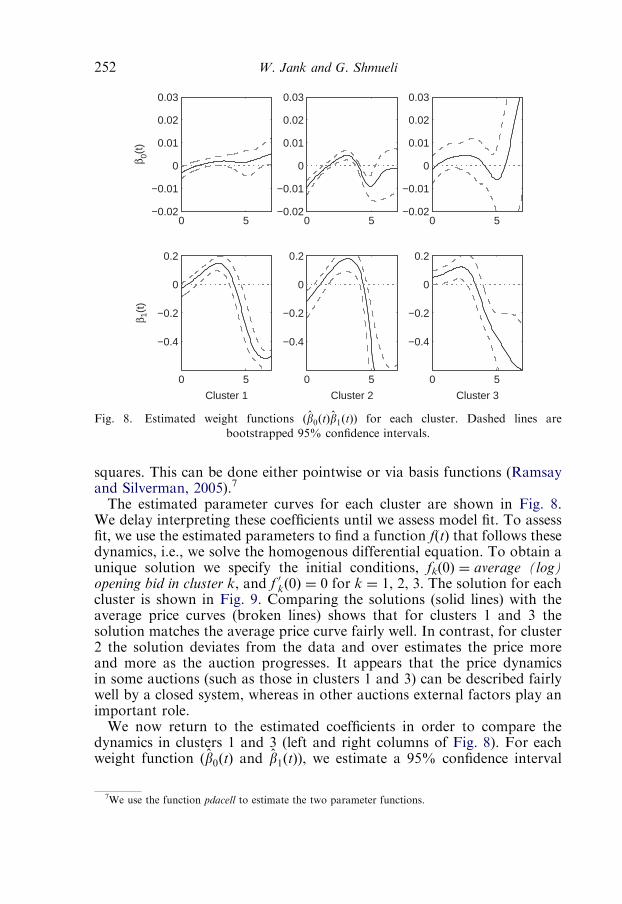
squares. This can be done either pointwise or via basis functions (Ramsayand Silverman, 2005).7
The estimated parameter curves for each cluster are shown in Fig. 8.We delay interpreting these coefficients until we assess model fit. To assessfit, we use the estimated parameters to find a function f(t) that follows thesedynamics, i.e., we solve the homogenous differential equation. To obtain aunique solution we specify the initial conditions, fk(0) ¼ average (log)opening bid in cluster k, and f 0kð0Þ ¼ 0 for k ¼ 1, 2, 3. The solution for eachcluster is shown in Fig. 9. Comparing the solutions (solid lines) with theaverage price curves (broken lines) shows that for clusters 1 and 3 thesolution matches the average price curve fairly well. In contrast, for cluster2 the solution deviates from the data and over estimates the price moreand more as the auction progresses. It appears that the price dynamicsin some auctions (such as those in clusters 1 and 3) can be described fairlywell by a closed system, whereas in other auctions external factors play animportant role.We now return to the estimated coefficients in order to compare the
dynamics in clusters 1 and 3 (left and right columns of Fig. 8). For eachweight function (b0ðtÞ and b1ðtÞ), we estimate a 95% confidence interval
0 5−0.02
−0.01
0
0.01
0.02
0.03
β 0(t)
0 5
−0.4
−0.2
0
0.2
Cluster 1
β 1(t
)
0 5−0.02
−0.01
0
0.01
0.02
0.03
0 5
−0.4
−0.2
0
0.2
Cluster 2
0 5−0.02
−0.01
0
0.01
0.02
0.03
0 5
−0.4
−0.2
0
0.2
Cluster 3
Fig. 8. Estimated weight functions ðb0ðtÞb1ðtÞÞ for each cluster. Dashed lines are
bootstrapped 95% confidence intervals.
7We use the function pdacell to estimate the two parameter functions.
W. Jank and G. Shmueli252
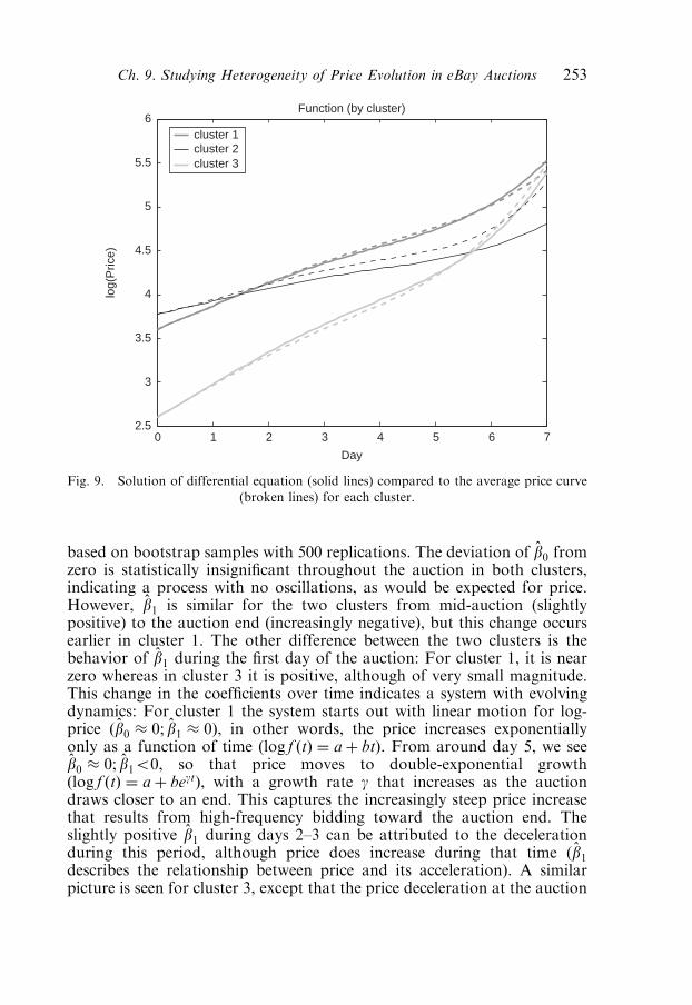
based on bootstrap samples with 500 replications. The deviation of b0 fromzero is statistically insignificant throughout the auction in both clusters,indicating a process with no oscillations, as would be expected for price.However, b1 is similar for the two clusters from mid-auction (slightlypositive) to the auction end (increasingly negative), but this change occursearlier in cluster 1. The other difference between the two clusters is thebehavior of b1 during the first day of the auction: For cluster 1, it is nearzero whereas in cluster 3 it is positive, although of very small magnitude.This change in the coefficients over time indicates a system with evolvingdynamics: For cluster 1 the system starts out with linear motion for log-price ðb0 0; b1 0Þ, in other words, the price increases exponentiallyonly as a function of time ðlog f ðtÞ ¼ aþ btÞ. From around day 5, we seeb0 0; b1o0, so that price moves to double-exponential growthðlog f ðtÞ ¼ aþ begtÞ, with a growth rate g that increases as the auctiondraws closer to an end. This captures the increasingly steep price increasethat results from high-frequency bidding toward the auction end. Theslightly positive b1 during days 2–3 can be attributed to the decelerationduring this period, although price does increase during that time (b1describes the relationship between price and its acceleration). A similarpicture is seen for cluster 3, except that the price deceleration at the auction
0 1 2 3 4 5 6 72.5
3
3.5
4
4.5
5
5.5
6Function (by cluster)
Day
log(
Pric
e)
cluster 1cluster 2cluster 3
Fig. 9. Solution of differential equation (solid lines) compared to the average price curve
(broken lines) for each cluster.
Ch. 9. Studying Heterogeneity of Price Evolution in eBay Auctions 253

start manifests itself as a positive b1. This can be seen when comparing theacceleration curves in Fig. 7.In conclusion, we learn that the price dynamics in auctions of clusters 1
and 3 can be described by a homogeneous differential equation of the formEq. (5). In both cases, price increases double exponentially from midauction, with an increasing growth rate. This occurs earlier in cluster 1 thanin 3. In contrast, the differential equation does not capture the dynamicsof cluster 2 auctions which may suggest that additional factors affect thesystem. Next, we examine such factors and their relation to the dynamics.
4.4 Comparing dynamic and non-dynamic cluster features
In order to gain insight into the relationship between price dynamics andother auction-related information we compare the three clusters withrespect to some key auction features. First, we compare the opening andclosing prices of the three clusters. Although the price curves approximatethe actual price during the auction relatively well, the actual price at theauction start and closing have special economic significance, which containadditional information about the price formation. Indeed, for our data wefind that the three clusters differ with respect to these prices. We investigateadditional auction characteristics that are relevant to the price formation:the day of the week that the auction closes, the seller’s rating (a proxy forreputation), the winner’s rating (a proxy for experience), the number of bidsand the number of distinct bidders that participated in the auction (bothproxies for competition). Table 1 gives summary statistics by cluster for allnumerical variables. Figure 10 compares the closing days of the threeclusters, and a w2 test (p-value ¼ 0.02) further confirms that cluster and day-of-week are statistically dependent.Table 1 and Fig. 10 suggest several possible strategies for bidding on an
auction. Take for instance auctions in cluster 2. These auctions arecharacterized by high opening bids, Tuesday closing days, and low final
Table 1
Summary statistics by cluster (on log scale)
Cluster Obid Price SelRate WinRate Nbids Nbidders ClusSize
1 Mean SE 6.98 234.86 40.70 34.04 10.79 6.19 90
1.43 1.01 1.13 1.19 1.13 1.10
2 Mean SE 6.18 216.30 26.43 32.13 17.16 8.27 47
1.66 1.02 1.20 1.28 1.10 1.10
3 Mean SE 0.17 233.04 20.52 22.41 24.87 12.53 46
1.63 1.01 1.15 1.29 1.06 1.05
Notes: Opening bid (Obid), closing price (Price), seller rating (SelRate), winner rating (WinRate), andnumber of bids and bidders (Nbids, Nbidders). ‘‘ClusSize’’ denotes the size of each cluster.
W. Jank and G. Shmueli254
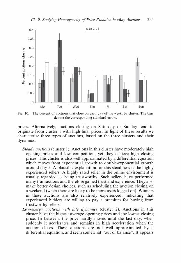
prices. Alternatively, auctions closing on Saturday or Sunday tend tooriginate from cluster 1 with high final prices. In light of these results wecharacterize three types of auctions, based on the three clusters and theirdynamics:
Steady auctions (cluster 1). Auctions in this cluster have moderately highopening prices and low competition, yet they achieve high closingprices. This cluster is also well approximated by a differential equationwhich moves from exponential growth to double-exponential growtharound day 5. A plausible explanation for this steadiness is the highlyexperienced sellers. A highly rated seller in the online environment isusually regarded as being trustworthy. Such sellers have performedmany transactions and therefore gained trust and experience. They alsomake better design choices, such as scheduling the auction closing ona weekend (when there are likely to be more users logged on). Winnersin these auctions are also relatively experienced, indicating thatexperienced bidders are willing to pay a premium for buying fromtrustworthy sellers.
Low-energy auctions with late dynamics (cluster 2). Auctions in thiscluster have the highest average opening prices and the lowest closingprice. In between, the price hardly moves until the last day, whensuddenly it accelerates and remains in high acceleration when theauction closes. These auctions are not well approximated by adifferential equation, and seem somewhat ‘‘out of balance’’. It appears
0
0.05
0.1
0.15
0.2
0.25
0.3
0.35
0.4
Sun
Per
cen
t au
ctio
ns
clo
sin
g
1 2 3
Mon Tue Wed Thu Fri Sat
Fig. 10. The percent of auctions that close on each day of the week, by cluster. The bars
denote the corresponding standard errors.
Ch. 9. Studying Heterogeneity of Price Evolution in eBay Auctions 255

that the high opening price deters potential bidders from participatingin the auction, and in turn the low competition level leads to lowerprices. Or perhaps there are other reasons that make these auctionsunattractive (e.g., they tend to end on a weekday).
Bazaar auctions (cluster 3). Auctions in this cluster are the most dynamic:the price increase moves quickly from exponential to double-exponential growth (and is well approximated by a differentialequation), with acceleration peaking early on and then again beforethe close. These auctions have, on average, the lowest opening price,the highest competition, and high closing prices. The low opening priceappears to be the only attractor of these auctions: sellers have lowratings and auctions close mostly on weekdays. We call them ‘‘bazaar’’auctions because the market place seems to work efficiently in reachingthe final price through dynamic competition.
4.5 A comparison with ‘‘traditional’’ clustering
Section 4.4 sheds light on auction dynamics and their relationship withother (static) auction information. We obtain this insight via curveclustering on the auction price processes. In the following we show theamount of information that is lost by not taking a functional approach, andinstead performing a traditional cluster analysis.The price curves describe the process of bidding between the start and end
of the auction. In contrast, a traditional approach ignores the price curvesand focuses only on the beginning and the end of this process, that is, on theopening bid and the final price only. We can think of this as a staticapproach since it ignores all the price dynamics. Table 2 shows the results ofsuch a static clustering approach. Using the same approach (including thesame K-medoids algorithm) as in Section 4.1, we obtain three clusters.Although cluster sizes are similar to those in Table 1 (90;47;46 vs. 93;45;45)the three clusters are in fact very different from those in Table 1.
Table 2
Cluster-specific summaries (similar to Table 1) for clustering on the opening bid and the final
price only
Cluster Obid Price SelRate WinRate Nbids Nbidders ClusSize
1 Mean SE 20.24 201.16 46.74 35.59 12.73 6.83 93
1.35 1.01 1.18 1.29 1.15 1.12
2 Mean SE 15.14 240.53 40.86 41.45 12.22 6.52 45
1.40 1.01 1.20 1.25 1.17 1.14
3 Mean SE 0.01 238.18 11.23 13.38 26.78 13.94 45
1.00 1.01 1.01 1.20 1.03 1.02
W. Jank and G. Shmueli256

In particular, they segment auctions into three groups, one with eBay’s‘‘default’’ opening bid of 0.01, one with medium, and one with high openingbids, but otherwise there is hardly any separation on the other dimensions.In fact, clusters 1 and 2 are almost identical with respect to seller rating,winner rating, and competition (number of bidders and bids). Furthermore,cluster variances are also much larger. The fact that competition is notcaptured by this static clustering can be attributed to the fact thatcompetition pertains to what happens during an auction and can thereforeonly be captured by the price curve. In contrast, the opening bid and thefinal price ignore competition and thus result in a loss of valuable auctioninformation.Another way of assessing the information loss due to a static clustering
approach is by looking at the dynamic price profiles. Figure 11 shows theprice curves and their dynamics (similar to Fig. 7) for the static clustering(i.e., using only opening bid and final price). The mean trend in the curves isgenerally comparable to the curve clustering result, but the inter-clusterheterogeneity is very large. The effect is especially notable in the velocityand acceleration.
5 Conclusions
In this study we take advantage of the wealth of high quality, publiclyavailable data that exist in the online marketplace, and discuss limitationsof some of the empirical research that has been conducted. In particular, thecurrent literature has focused on quantifying the relationship between thefinal price of an auction and factors such as competition, opening price, andclosing day. Although there is empirical evidence of different dynamics thattake place during an auction, and although these differing dynamics arelikely to affect the final price, there has been no attempt to quantify thesedynamics.We focus here on price formation processes in online auctions and their
dynamics and show that the price process in an online auction can bediverse even when dealing with auctions for very similar items with verysimilar settings. Using a functional representation of the price evolution,and functional data analytic tools, we find and characterize three ‘‘types’’ ofauctions that exhibit different price dynamics. These differences reflect orresult from different auction settings such as seller ratings, closing days,opening prices, and competition, but also from different dynamics that takeplace throughout the auction. We show that the static information alonedoes not fully explain the differences and leads to a loss of valuableinformation. Hence, the ability to couple static and dynamic sources ofinformation is important for better understanding the mechanics of onlineauctions.
Ch. 9. Studying Heterogeneity of Price Evolution in eBay Auctions 257

0 1 2 3 4 5 6 7
050
100
150
200
250
300
Price Process Cluster 1
Day of Auction
Pric
e
0 1 2 3 4 5 6 7
050
100
150
200
250
300
Price Process Cluster 2
Day of Auction
Pric
e
0 1 2 3 4 5 6 7
050
100
150
200
250
300
Price Process Cluster 3
Day of Auction
Pric
e
0 1 2 3 4 5 6 7
050
100
150
200
250
300
Price Process All Clusters
Day of Auction
Pric
e
0 1 2 3 4 5 6 7
0.0
0.2
0.4
0.6
0.8
1.0
Price Velocity Cluster 1
Day of Auction
Firs
t Der
ivat
ive
of L
og−
Pric
e
0 1 2 3 4 5 6 7
0.0
0.2
0.4
0.6
0.8
1.0
Price Velocity Cluster 2
Day of Auction
Firs
t Der
ivat
ive
of L
og−
Pric
e
0 1 2 3 4 5 6 7
0.0
0.2
0.4
0.6
0.8
1.0
Price Velocity Cluster 3
Day of Auction
Firs
t Der
ivat
ive
of L
og−
Pric
e
0 1 2 3 4 5 6 7
0.0
0.2
0.4
0.6
0.8
1.0
Price Velocity All Clusters
Day of Auction
Firs
t Der
ivat
ive
of L
og−
Pric
e
0 1 2 3 4 5 6 7
0.0
0.2
0.4
0.6
0.8
Price Acceleration Cluster 1
Day of Auction
Sec
ond
Der
ivat
ive
of L
og−
Pric
e
0 1 2 3 4 5 6 7
0.0
0.2
0.4
0.6
0.8
Price Acceleration Cluster 2
Day of Auction
Sec
ond
Der
ivat
ive
of L
og−
Pric
e
0 1 2 3 4 5 6 7
0.0
0.2
0.4
0.6
0.8
Price Acceleration Cluster 3
Day of Auction
Sec
ond
Der
ivat
ive
of L
og−
Pric
e
0 1 2 3 4 5 6 7
0.0
0.2
0.4
0.6
0.8
Price Acceleration Clusters
Day of Auction
Sec
ond
Der
ivat
ive
of L
og−
Pric
e
Fig. 11. Price profiles for clustering only on the starting- and the end-price.
W.JankandG.Shmueli
258
The combination of static information with price dynamics leads toresulting behavior that sometimes adheres to auction theory, whileothertimes it does not. For example, the three-way relationship betweenthe opening price, competition, and the final price, which has also beenshown empirically elsewhere (Bapna et al., 2008; Lucking-Reiley, 1999) istheoretically justified: Lower prices lead to more competition, which in turnresult in higher prices. However, we find that this three-way relationshipdiffers across clusters: it holds in ‘‘Bazaar auctions’’ and its reverse is true in‘‘low-energy auctions with late dynamics’’, but it does not hold in ‘‘Steadyauctions’’. In the latter it appears as if the experienced sellers are able toelicit higher prices (from more experienced winners) despite high openingprices and low competition. These conditional relationships were uncoveredby examining the price dynamics of the entire auction rather than theopening and closing price alone.Another well-known effect is the premium carried by experienced sellers
(Lucking-Reiley, 2000). We find evidence for this effect in some auctiontypes (‘‘steady auctions’’), but not in others (‘‘low energy with late dynamicsauctions’’).The existence of several auction types and the relationship between
auction characteristics and price dynamics can be of use to sellers, bidders,the auction house, and, in general, to decision makers in the onlinemarketplace. For instance, our results based on the Palm Pilot sampleindicate that low-rated sellers might be better off setting a low openingprice, a weekend closing, and other features that will increase competitionand result in high-price velocity at the end. Furthermore, on eBay, forexample, a seller is allowed to change the opening price and a few othersettings before the first bid is submitted. We can therefore imagine a systemwhere a seller evaluates, based on the dynamics in the beginning of his/herauction, what type of auction it is, and dynamically change the auctionsettings to improve dynamics.An auction house, like eBay, can use information on different types of
auction dynamics to decide on varying pricing strategies and to determineoptimal bid increments. Pricing strategies and bid increments affect theprice dynamics and their optimal choice could avoid the typical lack ofprice movements during the middle of an auction. Moreover, pricedynamics can be used to determine fraud. Fraudulent sellers could besuspected before the end of the transaction if their auction dynamics do notfollow typical patterns. Bidders could use differences in price dynamics toforecast the ending price of an auction. This information, in turn, can helpin deciding which auction to bid on among a large set of competingauctions for the same product (Wang et al., 2008).One of the limitations of the current approach is that it is only geared
toward auctions of a certain fixed duration (e.g., 7-day auctions). While thiscan be generalized to auctions of different durations (see Bapna et al.,2008), one distinct feature of eBay auctions is the fixed ending time. It is yet
Ch. 9. Studying Heterogeneity of Price Evolution in eBay Auctions 259

to be investigated how the same approach can be used for auctions withflexible ending times (e.g., Yahoo! or Amazon auctions). Another avenuefor future research is to investigate exactly what external factors affectauctions that do show less of a ‘‘closed system behavior’’ (e.g., those incluster 2). A first step in that direction is proposed in (Jank et al., 2008) whouse novel functional differential equation tree methodology to incorporatepredictor variables into dynamic models. Moreover, while we discussseveral possible implications of our work for the seller, the buyer and theauction house, a thorough exploitation of price dynamics for businessdecision making in the auction context has not been undertaken yet.In conclusion, new insights can be gained within the field of online
auctions by examining and modeling price dynamics or other dynamicprocesses through an FDA approach. In fact, a functional approach is verynatural in this digital era, where data tend to comprise of both longitudinaland cross-sectional information and often very tightly coupled (Jank andShmueli, 2006). Methods for exploring (e.g., Shmueli et al., 2006) andanalyzing such data are therefore likely to become a necessity.
References
Abraham, C., P.A. Cornillion, E. Matzner-Lober, N. Molinari (2003). Unsupervised curve-clustering
using b-spline. Scandinavian Journal of Statistics 30(3), 581–595.
Ba, S., P.A. Pavlou (2002). Evidence of the effect of trust building technology in electronic markets:
Price premiums and buyer behavior. MIS Quarterly 26, 269–289.
Bajari, P., A. Hortacsu (2003). The winner’s curse, reserve prices and endogenous entry: empirical
insights from ebay auctions. Rand Journal of Economics 3(2), 329–355.
Bapna, R., P. Goes, A. Gupta, Y. Jin (2004). User heterogeneity and its impact on electronic auction
market design: an empirical exploration. MIS Quarterly 28(1), 21–43.
Bapna, R., W. Jank, G. Shmueli (2008). Consumer surplus in online auctions. Information Systems
Research 19(4), December Issue.
Bapna, R., W. Jank, G. Shmueli (2008). Price formation and its dynamics in online auctions. Decision
Support Systems 44(3), 641–656.
Cuesta-Albertos, J.A., A. Gordaliza, C. Matran (1997). Trimmed k-means: an attempt to robustify
quantizers. The Annals of Statistics 25, 553–576.
Dellarocas, C. (2003). The digitization of word-of-mouth: promise and challenges of online reputation
mechanisms. Management Science 49, 1407–1442.
Hastie, T., R. Tibshirani, J. Friedman (2001). The Elements of Statistical Learning. Springer-Verlag,
New York.
Hastie, T.J., A. Buja, R.J. Tibshirani (1995). Penalized discriminant analysis. The Annals of Statistics 23,
73–102.
Hendricks, K., H.J. Paarsch (1995). A survey of recent empirical work concerning auctions. Canadian
Journal of Economics 28, 403–426.
Hyde, V., W. Jank, G. Shmueli (2006). Investigating concurrency in online auctions through
visualization. The American Statistician 60(3), 241–250.
James, G.M., C.A. Sugar (2003). Clustering sparsely sampled functional data. Journal of the American
Statistical Association 98, 397–408.
Jank, W., G. Shmueli (2006). Functional data analysis in electronic commerce research. Statistical
Science 21(2), 113–115.
W. Jank and G. Shmueli260

Jank, W., G. Shmueli, S. Wang (2008). Modeling price dynamics in online auctions via regression trees.
Jank, W. and Shmueli, G. (eds.), Statistical Methods in eCommerce Research, Wiley, New York.
Kaufman, L., P.J. Rousseeuw (1987). Clustering by means of medoids, in: Y. Dodge (ed.), Statistical
Data Analysis Based on the L1-norm and Related Methods. Elsevier, North-Holland, pp. 405–416.
Klein, S., R.M. O’Keefe (1999). The impact of the web on auctions: some empirical evidence and
theoretical considerations. International Journal of Electronic Commerce 3(3), 7–20.
Klemperer, P. (1999). Auction theory: a guide to the literature. Journal of Economic Surveys 13(3),
227–286.
Krishna, V. (2002). Auction Theory. Academic Press, San Diego.
Lucking-Reiley, D. (1999). Using field experiements to test equivalence between auction formats: magic
on the internet. American Economic Review 89(5), 1063–1080.
Lucking-Reiley, D. (2000). Auctions on the internet: what’s being auctioned and how? Journal of
Inductrial Economics 48(3), 227–252.
Milgrom, P., R. Weber (1982). A theory of auctions and competetive bidding. Econometrica 50(5),
1089–1122.
Pinker, E.J., A. Seidmann, Y. Vakrat (2003). Managing online auctions: current business and research
issues. Management Science 49, 1457–1484.
Ramsay, J.O., B.W. Silverman (2002). Applied functional data analysis: methods and case studies.
Springer-Verlag, New York.
Ramsay, J.O., B.W. Silverman (2005). Functional Data Analysis. 2nd ed. Springer Series in Statistics.
Springer-Verlag, New York
Roth, A.E., A. Ockenfels (2002). Last-minute bidding and the rules for ending second-price auctions:
evidence from ebay and amazon auctions on the internet. The American Economic Review 92(4),
1093–1103.
Ruppert, D., M.P. Wand, R.J. Carroll (2003). Semiparametric Regression. Cambridge University Press,
Cambridge.
Shmueli, G., W. Jank (2005). Visualizing online auctions. Journal of Computational and Graphical
Statistics 14(2), 299–319.
Shmueli, G., W. Jank, A. Aris, C. Plaisant, B. Shneiderman (2006). Exploring auction databases
through interactive visualization. Decision Support Systems 42(3), 1521–1538.
Shmueli, G., R.P. Russo, W. Jank (2007). The BARRISTA: a model for bid arrivals in online auctions.
Annals of Applied Statistics 1(2), 412–441.
Sugar, C.A., G.M. James (2003). Finding the number of clusters in a data set: an information theoretic
approach. Journal of the American Statistical Association 98, 750–763.
Tarpey, T., K.K.J. Kinateder (2003). Clustering functional data. Journal of Classification 20(1), 93–114.
Tibshirani, R., G. Walther, T. Hastie (2001). Estimating the number of clusters in a data set via the gap
statistic. Journal of the Royal Statistical Society Series B 63, 411–423.
Wang, S., W. Jank, G. Shmueli (2008). Explaining and forecasting ebay’s online auction prices using
functional data analysis. Journal of Business and Economic Statistics 26(2), 144–160.
Ch. 9. Studying Heterogeneity of Price Evolution in eBay Auctions 261

This page intentionally left blank
Adomavicius & Gupta, Eds., Handbooks in Information Systems, Vol. 3
Copyright r 2009 by Emerald Group Publishing Limited
Chapter 10
Scheduling Tasks Using Combinatorial Auctions:The MAGNET Approach$
John Collins and Maria GiniDepartment of Computer Science and Engineering, University of Minnesota, 200 Union St SE,
Room 4-192, Minneapolis, MN 55455, USA
Abstract
We consider the problem of rational, self-interested, economic agents whomust negotiate with each other in a market environment in order to carry outtheir plans. Customer agents express their plans in the form of task networkswith temporal and precedence constraints. A combinatorial reverse auctionallows supplier agents to submit bids specifying prices for combinations oftasks, along with time windows and duration data that the customer may useto compose a work schedule. We describe the consequences of allowing theadvertised task network to contain schedule infeasibilities, and show how toresolve them in the auction winner-determination process.
1 Introduction
We believe that much of the commercial potential of the Internet willremain unrealized until a new generation of autonomous systems isdeveloped and deployed. A major problem is that the global connectivityand rapid communication capabilities of the Internet can present anorganization with vast numbers of alternative choices, to the point thatusers are overwhelmed, and conventional automation is insufficient.Much has been done to enable simple buying and selling over the
Internet, and systems exist to help customers and suppliers find each other,such as search engines, vertical industry portals, personalization systems,and recommender engines. However, many business operations are much
$Work supported in part by the National Science Foundation under grants IIS-0084202 and
IIS-0414466.
263

more complex than the simple buying and selling of individual items.We are interested in situations that require coordinated combinations ofgoods and services, where there is often some sort of constraint-satisfactionor combinatorial optimization problem that needs to be solved in order toassemble a ‘‘deal.’’ Commonly, these extra complications are related toconstraints among task and services, and to time limitations. The combina-torics of such situations are not a major problem when an organization isworking with small numbers of partners, but can easily become nearlyinsurmountable when ‘‘opened up’’ to the public Internet.We envision a new generation of systems that will help organizations and
individuals find and exploit opportunities that are otherwise inaccessibleor too complex to seriously evaluate. These systems will help potentialpartners find each other (matchmaking), negotiate mutually beneficial deals(negotiation, evaluation, commitment), and help them monitor the progressof distributed activities (monitoring, dispute resolution). They will operatewith variable levels of autonomy, allowing their principals (users) todelegate or reserve authority as needed, and they will provide theirprincipals with a market presence and power that is far beyond what iscurrently achievable with today’s telephone, fax, web, and email-basedmethods. We believe that an important negotiation paradigm among thesesystems will be market-based combinatorial auctions, with added pre-cedence and temporal constraints.The multi-agent negotiation testbed (MAGNET) project represents a
first step in bringing this vision to reality. MAGNET provides a uniquecapability that allows self-interested agents to negotiate over complexcoordinated tasks, with precedence and time constraints, in an auction-based market environment. This chapter introduces many of the problemsa customer agent must solve in the MAGNET environment and exploresin detail the problem of solving the extended combinatorial-auction winner-determination problem.
Guide to this chapter: Section 2 works through a complete interactionscenario with an example problem, describing each of the decision processesa customer agent must implement in order to maximize the expected utilityof its principal. For some of them, we have worked out how to implementthe decisions, while for the remainder we only describe the problems.Section 3 focuses on one specific decision problem, that of deciding thewinners in a MAGNET auction. A number of approaches are possible; wedescribe an optimal tree search algorithm for this problem. Section 4 placesthis work in context with other work in the field. In particular, we draw onwork in multi-agent negotiation, auction mechanism design, and combina-torial-auction winner-determination, which has been a very active field inrecent years. Finally, Section 5 wraps up the discussion and points out a setof additional research topics that must be addressed to further realize theMAGNET vision.
J. Collins and M. Gini264
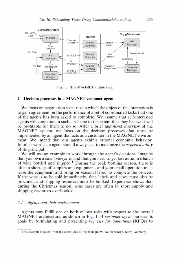
2 Decision processes in a MAGNET customer agent
We focus on negotiation scenarios in which the object of the interaction isto gain agreement on the performance of a set of coordinated tasks that oneof the agents has been asked to complete. We assume that self-interestedagents will cooperate in such a scheme to the extent that they believe it willbe profitable for them to do so. After a brief high-level overview of theMAGNET system, we focus on the decision processes that must beimplemented by an agent that acts as a customer in the MAGNET environ-ment. We intend that our agents exhibit rational economic behavior.In other words, an agent should always act to maximize the expected utilityof its principal.We will use an example to work through the agent’s decisions. Imagine
that you own a small vineyard, and that you need to get last autumn’s batchof wine bottled and shipped.1 During the peak bottling season, there isoften a shortage of supplies and equipment, and your small operation mustlease the equipment and bring on seasonal labor to complete the process.If the wine is to be sold immediately, then labels and cases must also beprocured, and shipping resources must be booked. Experience shows thatduring the Christmas season, wine cases are often in short supply andshipping resources overbooked.
2.1 Agents and their environment
Agents may fulfill one or both of two roles with respect to the overallMAGNET architecture, as shown in Fig. 1. A customer agent pursues itsgoals by formulating and presenting requests for quotations (RFQs) to
Top−LevelGoal
MarketOntology
MarketStatistics
MarketSession
TaskNetwork
DomainModel
Statistics
BidProtocol
Events &Responses
Re−Plan
BidManager
ExecutionManager
BidManager
ResourceManager
BidProtocol
Events &Responses
DomainModel
Commitments
Availability
Re−Bid
Customer Agent
MarketPlanner
TaskAssignment
Supplier Agent
Fig. 1. The MAGNET architecture.
1This example is taken from the operations of the Weingut W. Ketter winery, Krov, Germany.
Ch. 10. Scheduling Tasks Using Combinatorial Auctions 265

supplier agents through a market infrastructure (Collins et al., 1998). AnRFQ specifies a task network that includes task descriptions, a precedencenetwork, and temporal constraints that limit task start and completiontimes. Customer agents attempt to satisfy their goals for the greatestexpected profit, and so they will accept bids at the least net cost, where costfactors can include not only bid prices, but also goal completion time, riskfactors, and possibly other factors, such as preferences for specific suppliers.More precisely, these agents are attempting to maximize the utility functionof some user, as discussed in detail in Collins et al. (2000).A supplier agent attempts to maximize the value of the resources under its
control by submitting bids in response to customer RFQs. A bid specifieswhat tasks the supplier is able to undertake, when it is available to performthose tasks, how long they will take to complete, and a price. Each bid mayspecify one or more tasks. Suppliers may submit multiple bids to specifydifferent combinations of tasks, or possibly different time constraints withdifferent prices. For example, a supplier might specify a short duration forsome task that requires use of high cost overtime labor, as well as a longerduration at a lower cost using straight-time labor. MAGNET currentlysupports simple disjunction semantics for bids from the same supplier. Thismeans that if a supplier submits multiple bids, any non-conflicting subsetcan be accepted. Other bid semantics are also possible (Boutilier and Hoos,2001; Nisan, 2000a).
2.2 Planning
A transaction (or possibly a series of transactions) starts when the agentis given a goal that must be satisfied. Attributes of the goal might includea payoff and a deadline, or a payoff function that varies over time.While it would certainly be possible to integrate a general-purpose
planning capability into a MAGNET agent, we expect that in many realisticsituations the principal will already have a plan, perhaps based on standardindustry practices. Figure 2 shows such a plan for our winery bottlingoperation. We shall use this plan to illustrate the decision processes theagent must perform.Formally, we define a plan Pð¼ S;VÞ as a task network containing a set
of tasks S , and a set of precedence relations V. A precedence relation relates
Deliver bottles
Deliver cork
Print cases
Print labels
Deliver cases Pack cases Ship cases
begi
n
dead
lineBottle wine
Apply labels
Fig. 2. Plan for the wine-bottling example.
J. Collins and M. Gini266

two tasks s; s0 2 S as s � s0, interpreted as ‘‘task s must be completedbefore task s0 can start.’’We assume that markets will be sponsored by trade associations and
commercial entities, and will therefore be more or less specialized. Aconsequence of this is that agents must in general deal with multiplemarkets to accomplish their goals. For our example, we assume that thetasks in our plan are associated with markets as specified in Table 1.It appears that we will need to deal with three different markets, and we
will pack the cases ourselves. Or perhaps we will open a few bottles andinvite the village to help out.So far, our plan is not situated in time, and we have not discussed our
expected payoff for completing this plan. In the wine business, the qualityand value of the product depends strongly on time. The wine must beremoved from the casks within a 2-week window, and the bottling must bedone immediately.For some varieties, the price we can get for our wine is higher if we can
ship earlier, given a certain quality level. All the small vineyards in theregion are on roughly the same schedule, so competition for resourcesduring the prime bottling period can be intense. Without specifying theexact functions, we assume that the payoff drops off dramatically if we missthe 2-week bottling window, and less dramatically as the shipment daterecedes into the future.This example is of course simplified to demonstrate our ideas. For
example, we are treating the bottling and labeling operations as atomic—the entire bottling operation must be finished before we can start labeling—even though common-sense would inform us that we would probably wantto apply this constraint to individual bottles, rather than to the entire batch.However, some varieties of wine are aged in the bottles for 6 months ormore before the labels are applied.
Table 1
Tasks and market associations for the wine-bottling example
Task Description Market
s1 Deliver bottles Vineyard services
s2 Deliver cork Vineyard services
s3 Bottle wine Vineyard services
s4 Print labels Printing and graphic arts
s5 Apply labels Vineyard services
s6 Print cases Vineyard services
s7 Deliver cases Vineyard services
s8 Pack cases (none)
s9 Ship cases Transport services
Ch. 10. Scheduling Tasks Using Combinatorial Auctions 267

2.3 Planning the bidding process
At this point, the agent has a plan, and it knows which markets it mustdeal in to complete the plan. It also knows the value of completing the plan,and how that value depends on time. The next step is to decide how best touse the markets to maximize its utility. It will do this in two phases. First,the agent generates an overall plan for the bidding process, whichmay involve multiple RFQs in each of multiple markets. We call this a‘‘bid-process plan.’’ Then a detailed timeline is generated for each RFQ.The simplest bid-process plan would be to issue a single RFQ in each
market, each consisting of the portion of the plan that is relevant to itsrespective market. If all RFQs are issued simultaneously, and if they areall on the same timeline, then we can combine their bids and solve thecombined winner-determination problem in a single step. However, thismight not be the optimum strategy. For example,
� We may not have space available to store the cases if we are not readyto pack them when they arrive.� Our labor costs might be much lower if we can label as we bottle;otherwise, we will need to move the bottles into storage as we bottle,then take them back out to label them.� Once cases are packed, it is easy for us to store them for a short period.This means that we can allow some slack between the packing andshipping tasks.� There is a limit to what we are willing to pay to bottle our wine, andthere is a limit to the premium we are willing to pay to have thebottling completed earlier.
The agent can represent these issues as additional constraints on the plan,or in some cases as alternative plan components. For example, we couldconstrain the interval between s5 (labeling) and s8 (packing) to a maximumof one day, or we could add an additional storage task between s3 (bottling)and s5 that must be performed just in case there is a non-zero delay betweenthe end of s3 and the start of s5.There are many possible alternative actions that the agent can take to
deal with these issues. It need not issue RFQs in all markets simultaneously.It need not include all tasks for a given market in a single RFQ.Indeed, dividing the plan into multiple RFQs can be an important way toreduce scheduling uncertainty. For example, we might want to have a firmcompletion date for the bottling and labeling steps before we order thecases. When a plan is divided into multiple RFQs that are negotiatedsequentially, then the results of the first negotiation provide additionalconstraints on subsequent negotiations.Market statistics can be used to support these decisions. For example,
if we knew that resources were readily available for the steps up throughthe labeling process (tasks s1 . . . s5), we could include the case delivery and
J. Collins and M. Gini268

printing steps (tasks s6 and s7) in the same RFQ. This could beadvantageous if suppliers were more likely to bid or likely to bid lowerprices if they could bid on more of the business in a single interaction.In other words, some suppliers might be willing to offer a discount if weagree to purchase both bottles and cases from them, but if we negotiatethese two steps in separate RFQs, we eliminate the ability to find out aboutsuch discounts.We should note that suppliers can either help or hinder the customer in
this process, depending on the supplier’s motivations. For example, thesupplier can help the customer mitigate issues like the constraint betweenbottling and packing. For example, if a supplier knew about this constraint,it could offer both tasks at appropriate times, or it could give the customerthe needed scheduling flexibility by offering the case delivery over a broadtime window or with multiple bids with a range of time windows. In somedomains this could result in higher costs, due to the large speculativeresource reservations the supplier would have to commit in order to supportits bids. However, if a supplier saw an RFQ consisting of s6 and s7, it wouldknow that the customer had likely already made commitments for theearlier tasks, since nobody wants cases printed if they are not bottling.If the supplier also knew that there would be little competition within thecustomer’s specified time window, it could inflate its prices, knowing thatthe customer would have little choice.The bid-process plan that results from this decision process is a network
of negotiation tasks and decision points. Figure 3 shows a possible bid-process plan for our wine-bottling example.Once we have a bid-process plan, we know what markets we will operate
in, and how we want to divide up the bidding process. We must then
start
RFQ: r2Market: Printing & Graphic ArtsTasks: s4
acceptable? alert user
RFQ: r4Market: Transport ServicesTasks: s9
finish
RFQ: r1Market: Vineyard ServicesTasks: s1. . . s5
RFQ: r3Market: Vineyard ServicesTasks: s6. . . s7
no
yes
Fig. 3. Bid-process plan for the wine-bottling example.
Ch. 10. Scheduling Tasks Using Combinatorial Auctions 269

schedule the bid-process plan, and allocate time within each RFQ/biddinginteraction. These two scheduling problems may need to be solved togetherif the bid-process plan contains multiple steps and it is important to finishit in minimum time. Each RFQ step needs to start at a particular time, orwhen a particular event occurs or some condition becomes true. Forexample, if the rules of the market require deposits to be paid when bids areawarded, the customer may be motivated to move RFQ steps as late aspossible, other factors being equal. However, if resources such as ourbottling and labeling steps are expected to be in short supply, the agent maywish to gain commitments for them as early as possible in order to optimizeits own schedule and payoff. We assume these decisions can be supportedby market statistics, the agent’s own experience, and/or the agent’sprincipal.Each RFQ must also be allocated enough time to cover the necessary
deliberation processes on both the customer and supplier sides. Some ofthese processes may be automated, and some may involve user interaction.The timeline in Fig. 4 shows an abstract view of the progress of a singlenegotiation. At the beginning of the process, the customer agent mustallocate deliberation time to itself to compose its RFQ,2 to the supplier forbid preparation, and to itself again for the bid-evaluation process. Two ofthese time points, the bid deadline and the bid award deadline, must becommunicated to suppliers as part of the RFQ. The bid deadline is thelatest time a supplier may submit a bid, and the bid award deadline is theearliest time a supplier may expire a bid. The interval between these twotimes is available to the customer to determine the winners of the auction.In general, it is expected that bid prices will be lower if suppliers have
more time to prepare bids, and more time and schedule flexibility in theexecution phase. Minimizing the delay between the bid deadline and theaward deadline will also minimize the supplier’s opportunity cost, andwould therefore be expected to reduce bid prices. However, the customer’s
Supplier deliberates
Customer deliberates
Com
pose
RF
Q
Pla
n co
mpl
etio
n
Ear
liest
sta
rt o
fta
sk e
xecu
tion
dead
line
Bid
Aw
ard
Bid
dea
dlin
e
Sen
d R
FQ
Fig. 4. Typical timeline for a single RFQ.
2This may be a significant combinatorial problem—see for example Babanov et al. (2003).
J. Collins and M. Gini270
ability to find a good set of bids is dependent on the time allocated to bidevaluation, and if a user is making the final decision on bid awards, she maywant to run multiple bid-evaluation cycles with some additional think time.We are interested in the performance of the winner-determination processprecisely because it takes place within a window of time that must bedetermined ahead of time, before bids are received, and because we expectbetter overall results, in terms of maximizing the agent’s utility, if we canmaximize the amount of time available to suppliers while minimizingthe time required for customer deliberation. These time intervals can beoverlapped to some extent, but doing so can create opportunities forstrategic manipulation of the customer by the suppliers, as discussed inCollins et al. (1997).The process for setting these time intervals could be handled as a non-
linear optimization problem, although it may be necessary to settle for anapproximation. This could consist of estimating the minimum time requiredfor the customer’s processes, and allocating the remainder of the availabletime to the suppliers, up to some reasonable limit.
2.4 Composing a request for quotes
At this point in the agent’s decision process, we have the informationneeded to compose one or more RFQs, we know when to submit them, andwe presumably know what to do if they fail (if we fail to receive a bid setthat covers all the task in the RFQ, for example). The next step is to set thetime windows for tasks in the individual RFQs, and submit them to theirrespective markets.Formally, an RFQ r ¼ ðSr; Vr;Wr; tÞ contains a subset Sr of the tasks in
the task network P, with their precedence relations Vr, the task timewindows Wr specifying constraints on when each task may be started andcompleted, and the RFQ timeline t containing at least the bid deadline andbid award deadline. As we discussed earlier, there might be elements of thetask network P that are not included in the RFQ. For each task sASr, inthe RFQ we must specify a time window w 2Wr, consisting of an earlieststart time tes (s, r) and a latest finish time tlf (s, r), and a set of precedencerelationships Vr ¼ fs0 2 Sr; s0 � sg, associating s with each of the other taskss0 2 Sr; whose completion must precede the start of s.The principal outcome of the RFQ-generation process is a set of values
for the early-start and late-finish times for the time windows Wr in theRFQ. We obtain a first approximation using the critical path (CPM)algorithm (Hillier and Lieberman, 1990), after making some assumptionsabout the durations of tasks, and about the earliest start time for tasks thathave no predecessors in the RFQ (the root tasks SR) and the latest finishtimes for tasks that have no successors in the RFQ (the leaf tasks SL).Market mean-duration statistics could be used for the task durations.
Ch. 10. Scheduling Tasks Using Combinatorial Auctions 271
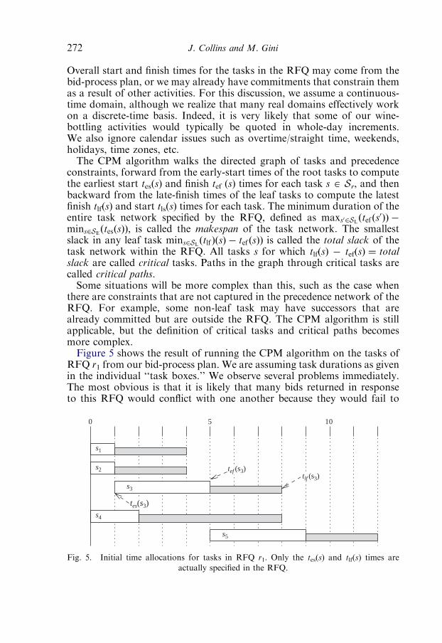
Overall start and finish times for the tasks in the RFQ may come from thebid-process plan, or we may already have commitments that constrain themas a result of other activities. For this discussion, we assume a continuous-time domain, although we realize that many real domains effectively workon a discrete-time basis. Indeed, it is very likely that some of our wine-bottling activities would typically be quoted in whole-day increments.We also ignore calendar issues such as overtime/straight time, weekends,holidays, time zones, etc.The CPM algorithm walks the directed graph of tasks and precedence
constraints, forward from the early-start times of the root tasks to computethe earliest start tes(s) and finish tef (s) times for each task s A Sr, and thenbackward from the late-finish times of the leaf tasks to compute the latestfinish tlf(s) and start tls(s) times for each task. The minimum duration of theentire task network specified by the RFQ, defined as maxs02SLðtef ðs
0ÞÞ �
mins2SEðtesðsÞÞ; is called the makespan of the task network. The smallestslack in any leaf task mins2SLðtlf ÞðsÞ � tef ðsÞÞ is called the total slack of thetask network within the RFQ. All tasks s for which tlf(s) � tef(s) ¼ totalslack are called critical tasks. Paths in the graph through critical tasks arecalled critical paths.Some situations will be more complex than this, such as the case when
there are constraints that are not captured in the precedence network of theRFQ. For example, some non-leaf task may have successors that arealready committed but are outside the RFQ. The CPM algorithm is stillapplicable, but the definition of critical tasks and critical paths becomesmore complex.Figure 5 shows the result of running the CPM algorithm on the tasks of
RFQ r1 from our bid-process plan. We are assuming task durations as givenin the individual ‘‘task boxes.’’ We observe several problems immediately.The most obvious is that it is likely that many bids returned in responseto this RFQ would conflict with one another because they would fail to
0150
s4
s5
s1
s2
s3
tef (s3)
tes(s3)
tlf (s3)
Fig. 5. Initial time allocations for tasks in RFQ r1. Only the tes(s) and tlf(s) times are
actually specified in the RFQ.
J. Collins and M. Gini272

combine feasibly. For example, if I had a bid for the label-printing task s4for days 5–7, then the only bids I could accept for the labeling task s5 wouldbe those that had a late start time at least as late as day 7. If the bids for s5were evenly distributed across the indicated time windows, and if all ofthem specified the same 4-day duration, then only 1/3 of those bids could beconsidered. In general, we want to allow time windows to overlap, butexcessive overlap is almost certainly counterproductive. We will revisit thisissue shortly.Once we have initial estimates from the CPM algorithm, there are several
issues to be resolved, as described in the following sections.
2.4.1 Setting the total slackThe plan may have a hard deadline, which may be set by a user or
determined by existing commitments for tasks that cannot be started untiltasks in the current RFQ are complete. Otherwise, in the normal case, thebid-process plan is expected to set the time limits for the RFQ.It would be interesting to find a way to use the market to dynamically
derive a schedule that maximizes the customer’s payoff. This would requirecooperation of bidders, and could be quite costly. Parkes and Ungar (2001)have done something like this in a restricted domain, but it is hard to seehow to apply it to the more generalized MAGNET domain.
2.4.2 Task orderingFor any pair of tasks in the plan that could potentially be executed in
parallel, we may have a choice of handling them either in parallel, or insequential order. For example, in our wine-bottling example, we couldchoose to acquire the bottles before buying the corks. In general, if there isuncertainty over the ability to complete tasks which could cause the plan tobe abandoned, then (given some straightforward assumptions such aspayments being due when work is completed) the agent’s financial exposurecan be affected by task ordering. If a risky task is scheduled ahead of a‘‘safe’’ task, then if the risky task fails we can abandon the plan withouthaving to pay for the safe task. Babanov et al. (2003) have worked out indetail how to use task completion probabilities and discount rates in anexpected-utility framework to maximize the probabilistic ‘‘certain payoff ’’for an agent with a given risk-aversion coefficient.For some tasks, linearizing the schedule will extend the plan’s makespan,
and this must be taken into account in terms of changes to the ultimatepayoff. Note that in many cases the agent may have flexibility in the starttime as well as the completion time of the schedule. This would presumablybe true of our wine-bottling example.
2.4.3 Allocating time to individual tasksOnce we have made decisions about the overall time available and about
task ordering, the CPM algorithm gives us a set of preliminary time
Ch. 10. Scheduling Tasks Using Combinatorial Auctions 273
windows. In most cases, this will not produce the best results, for severalreasons.
Resource availability. In most markets, services will vary in terms ofavailability and resource requirements. There may be only a few dozenportable bottling and labeling machines in the region, while corks may bestored in a warehouse ready for shipping. There is a high probability thatone could receive several bids for delivery of corks on one specific day, but amuch lower probability that one could find even 1 bid for a 6-day bottlingjob for a specific 6-day period. More likely one would have to allow someflexibility in the timing of the bottling operation in order to receive usablebids.
Lead-time effects. In many industries, suppliers have resources on thepayroll that must be paid for whether their services are sold or not. In thesecases, suppliers will typically attempt to ‘‘book’’ commitments for theirresources into the future. In our example, the chances of finding a printshop to produce our labels tomorrow is probably much lower than thechances of finding shops to print them next month. This means that, at leastfor some types of services, one must allow more scheduling flexibility toattract short lead-time bids than for longer lead times. We should alsoexpect to pay more for shorter lead times.
Task-duration variability. Some services are very standardized (deliveringcorks, printing 5000 labels), while others may be highly variable, eitherbecause they rely on human creativity (software development) or theweather (bridge construction), or because different suppliers use differentprocesses, different equipment, or different staffing levels (wine bottling).These two types of variability can usually be differentiated by the level ofpredictability; suppliers that uses a predictable process with variablestaffing levels are likely to be able to deliver on time on a regular basis,while services that are inherently unpredictable will tend to exhibit frequentdeviations from the predictions specified in bids.3 For services that exhibit ahigh variability in duration, as specified in bids, the customer’s strategy maydepend on whether a large number of bidders is expected, and whether thereis a correlation between bid price and quoted task duration. If a largenumber of bidders is expected, then the customer may be able to allocate abelow-average time window to the task, in the expectation that there will besome suppliers at the lower end of the distribution who will be able toperform within the specified window. However, if few bidders are expected,a larger than average time window may be required in order to achieve areasonable probability of receiving at least one usable bid.
3Whether the market or customers would be able to observe these deviations may depend on marketrules and incentives, such as whether a supplier can be paid early by delivering early.
J. Collins and M. Gini274

Excessive allocations to non-critical tasks. One obvious problem with thetime allocations from the CPM algorithm as shown in Fig. 5 is that non-critical tasks (tasks not on the critical path) are allocated too much time,causing unnecessary overlap in their time windows. All other things beingequal, we are likely to be better off if RFQ time windows do not overlap,because we will have fewer infeasible bid combinations.
2.4.4 Trading off feasibility for flexibilityIn general we expect more bidders, and lower bid prices, if we offer
suppliers more flexibility in scheduling their resources by specifying widertime windows. However, if we define RFQ time windows with excessiveoverlap, a significant proportion of bid combinations will be unusable dueto schedule infeasibility. The intuition is that there will be some realisticmarket situations where the customer is better off allowing RFQ timewindows to overlap to some degree, if we take into account price, plancompletion time, and probability of successful plan completion(which requires at minimum a set of bids that covers the task set and canbe composed into a feasible schedule). This means that the winner-determination procedure must handle schedule infeasibilities among bids.Figure 6 shows a possible updated set of RFQ time windows for our
wine-bottling example, taking into account the factors we have discussed.We have shortened the time windows for tasks s1 and s2, because we believethat bottles and corks are readily available, and can be delivered whenneeded. There is no advantage in allowing more time for these tasks.Market data tells us that bottling services are somewhat more difficult toschedule than labeling services, and so we have specified a wider timewindow for task s3 than for s4. Our deadline is such that the value ofcompleting the work a day or two earlier is higher than the potential loss ofhaving to reject some conflicting bids. We also know from market data thata large fraction of suppliers of the bottling crews can also provide thelabeling service, and so the risk of schedule infeasibility will be reduced if we
s4
s5
015
s1
s2
s3
0
Fig. 6. Revised time allocations for tasks in RFQ r1.
Ch. 10. Scheduling Tasks Using Combinatorial Auctions 275
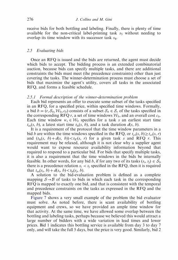
receive bids for both bottling and labeling. Finally, there is plenty of timeavailable for the non-critical label-printing task s5 without needing tooverlap its time window with its successor task s4.
2.5 Evaluating bids
Once an RFQ is issued and the bids are returned, the agent must decidewhich bids to accept. The bidding process is an extended combinatorialauction, because bids can specify multiple tasks, and there are additionalconstraints the bids must meet (the precedence constraints) other than justcovering the tasks. The winner-determination process must choose a set ofbids that maximize the agent’s utility, covers all tasks in the associatedRFQ, and forms a feasible schedule.
2.5.1 Formal description of the winner-determination problemEach bid represents an offer to execute some subset of the tasks specified
in an RFQ, for a specified price, within specified time windows. Formally,a bid b ¼ ðr;Sb;Wb; cbÞ consists of a subset Sb 2 Sr of the tasks specified inthe corresponding RFQ r, a set of time windowsWb, and an overall cost cb.Each time window ws 2Wb specifies for a task s an earliest start timetes(s, b), a latest start time tls(s, b), and a task duration d(s, b).It is a requirement of the protocol that the time window parameters in a
bid b are within the time windows specified in the RFQ, or tes(s, b)Ztes(s, r)and (tls(s, b)þ d(s, b))otlf (s, r) for a given task s and RFQ r. Thisrequirement may be relaxed, although it is not clear why a supplier agentwould want to expose resource availability information beyond thatrequired to respond to a particular bid. For bids that specify multiple tasks,it is also a requirement that the time windows in the bids be internallyfeasible. In other words, for any bid b, if for any two of its tasks (si, sj) A Sbthere is a precedence relation si � sj specified in the RFQ, then it is requiredthat tes(si, b)þ d(si, b)otls(sj, b).A solution to the bid-evaluation problem is defined as a complete
mapping S-B of tasks to bids in which each task in the correspondingRFQ is mapped to exactly one bid, and that is consistent with the temporaland precedence constraints on the tasks as expressed in the RFQ and themapped bids.Figure 7 shows a very small example of the problem the bid evaluator
must solve. As noted before, there is scant availability of bottlingequipment and crews, so we have provided an ample time window forthat activity. At the same time, we have allowed some overlap between thebottling and labeling tasks, perhaps because we believed this would attract alarge number of bidders with a wide variation in lead times and lowerprices. Bid 1 indicates this bottling service is available from day 3 to day 7only, and will take the full 5 days, but the price is very good. Similarly, bid 2
J. Collins and M. Gini276

offers labeling from day 7 to day 10 only, again for a good price.Unfortunately, we cannot use these two bids together because of theschedule infeasibility between them. Bid 3 offers bottling for any 3-dayperiod from day 2 to day 7, at a higher price. We can use this bid with bid 2if we start on day 4, but if we start earlier we will have to handle theunlabeled bottles somehow. Finally, bid 4 offers both the bottling andlabeling services, but the price is higher and we would finish a day later thanif we accepted bids 2 and 3.
2.5.2 Evaluation criteriaWe have discussed the winner-determination problem in terms of price,
task coverage, and schedule feasibility. In many situations, there are otherfactors that can be at least as important as price. For example, we mightknow (although the agent might not know) that the bottling machine beingoffered in bid 3 is prone to breakdown, or that it tends to spill a lot of wine.We might have a long-term contract with one of the suppliers, Hermann,that gives us a good price on fertilizer only if we buy a certain quantity ofcorks from him every year. We might also know that one of the localprinters tends to miss his time estimates on a regular basis, but his prices areoften worth the hassle, as long as we build some slack into the schedulewhen we award a bid to him.Of course, including these other factors will distort a ‘‘pure’’ auction
market, since the lowest-price bidder will not always win. As a practicalmatter, such factors are commonly used to evaluate potential procurement
RFQTime windows
0150
s3 (bottling)
s4 (labeling)
Bid 2
Bid 3
labeling, 300$
tes(s3, b3)
bottling & labeling, 1200$
Bid 4
Bid 1 bottling, 500$
bottling, 800$
d(s3, b3)
tls(s3, b3)
Fig. 7. Bid example.
Ch. 10. Scheduling Tasks Using Combinatorial Auctions 277

decisions, and real market mechanisms must include them if they are to bewidely acceptable.Many of these additional factors can be expressed as additional con-
straints on the winner-determination problem, and some can be expressedas cost factors. These constraints can be as simple as ‘‘don’t use bid b3’’ ormore complex, as in ‘‘if Hermann bids on corks, and if a solution using hisbid is no more than 10% more costly than a solution without his bid, thenaward the bid to Hermann.’’Some of them can be handled by preprocessing, some must be handled
within the winner-determination process, and some will require running itmultiple times and comparing results.
Mixed-initiative approaches. There are many environments in which anautomated agent is unlikely to be given the authority to make unsupervisedcommitments on behalf a person or organization. In these situations, weexpect that many of the decision processes we discuss here will be used asdecision-support tools for a human decision-maker, rather than as elementsof a completely autonomous agent. The decision to award bids is one thatdirectly creates commitment, and so it is a prime candidate for userinteraction. We have constructed an early prototype of such an interface.It allows a user to view bids, add simple bid inclusion and exclusionconstraints, and run one of the winner-determination search methods. Bidsmay be graphically overlaid on the RFQ, and both the RFQ and bid timewindows are displayed in contrasting colors on a Gantt-chart display.Effective interactive use of the bid-evaluation functions of an agent
require the ability to visualize the plan and bids, to visualize bids in groupswith constraint violations highlighted, and to add and update constraints.The winner-determination solver must be accessible and its resultspresented in an understandable way, and there must be a capability togenerate multiple alternative solutions and compare them.
2.6 Awarding bids
The result of the winner-determination process is a (possibly empty)mapping S! B of tasks to bids. We assume that the bids in this mappingmeet the criteria of the winner-determination process: they cover the tasksin the RFQ, can be composed into a feasible schedule, and they maximizethe agent’s or user’s expected utility. However, we cannot just award thewinning bids. In general, a bid b contains one or more offers of services fortasks s, each with a duration d(s, b) within a time window w(s, b) W d(s, b).The price assumes that the customer will specify, as part of the bid award, aspecific start time for each activity. Otherwise, the supplier would have tomaintain its resource reservation until some indefinite future time when thecustomer would specify a start time. This would create a disincentive for
J. Collins and M. Gini278

suppliers to specify large time windows, raise prices, and complicate thecustomer’s scheduling problem.This means that the customer must build a final work schedule before
awarding bids. We will defer the issue of dealing with schedule changes aswork progresses. This scheduling activity represents another opportunity tomaximize the customer’s expected utility. In general, the customer’s utilityat this point is maximized by appropriate distribution of slack in theschedule, and possibly also by deferring task execution in order to deferpayment for completion.
3 Solving the MAGNET winner-determination problem
We now focus on the MAGNET winner-determination problem,originally introduced in Section 2.5. Earlier we have described both anInteger Programming formulation (Collins and Gini, 2001) and a simulatedannealing framework for solving this problem (Collins et al., 2001). Inthis chapter, we describe an application of the A� method (Russell andNorvig, 1995). For simplicity, the algorithm presented here solves thewinner-determination problem assuming that the payoff does not dependon completion time.The A� algorithm is a method for finding optimal solutions to
combinatorial problems that can be decomposed into a series of discretesteps. A classic example is finding the shortest route between two points in aroad network. A� works by constructing a tree of partial solutions. Ingeneral, tree search methods such as A� are useful when the problem can becharacterized by a solution path in a tree that starts at an initial node (root)and progresses through a series of expansions to a final node that meets thesolution criteria. Each expansion generates successors (children) of someexisting node, expansions continuing until a solution node is found. Thequestions of which node is chosen for expansion, and how the search tree isrepresented, lead to a family of related search methods. In the A� method,the node chosen for expansion is the one with the ‘‘best’’ evaluation,4 andthe search tree is typically kept in memory in the form of a sorted queue. A�
uses an evaluation function
f ðNÞ ¼ gðNÞ þ hðNÞ (1)
for a node N, where g(N) is the cost of the path from initial node N0 to nodeN, and h(N) is an estimate of the remaining cost to a solution node. If h(N)is a strict lower bound on the remaining cost (upper bound for amaximization problem), we call it an admissible heuristic and A� is completeand optimal; that is, it is guaranteed to find a solution with the lowest
4Lowest for a minimization problem, highest for a maximization problem.
Ch. 10. Scheduling Tasks Using Combinatorial Auctions 279

evaluation, if any solutions exist, and it is guaranteed to terminateeventually if no solutions exist.The winner-determination problem for combinatorial auctions has been
shown to be NP-complete and inapproximable (Sandholm, 1999). Thisresult clearly applies to the MAGNET winner-determination problem,since we simply apply an additional set of (temporal) constraints to thebasic combinatorial-auction problem, and we do not allow free disposal(because we want a set of bids that covers all tasks). In fact, because theadditional constraints create additional bid-to-bid dependencies, andbecause bids can vary in both price and in time specifications, the bid-domination and partitioning methods used by others to simplify theproblem (for example, see Sandholm, 2002) cannot be applied in theMAGNET case.Sandholm has shown that there can be no polynomial-time solution, nor
even a polynomial-time bounded approximation (Sandholm, 2002), so wemust accept exponential complexity. We have shown in Collins (2002)that we can determine probability distributions for search time, basedon problem size metrics, and we can use those empirically determineddistributions in our deliberation scheduling process.Sandholm described an approach to solving the standard combinatorial-
auction winner-determination problem (Sandholm, 2002) using an iterative-deepening A� formulation. Although many of his optimizations, such as theelimination of dominated bids and partitioning of the problem, cannotbe easily applied to the MAGNET problem, we have adapted the basicstructure of Sandholm’s formulation, and we have improved upon it byspecifying a means to minimize the mean branching factor in the generatedsearch tree.We describe a basic A� formulation of theMAGNET winner-determination
problem, and then we show how this formulation can be adapted toa depth-first iterative-deepening model (Korf, 1985) to reduce or eliminatememory limitations.
3.1 Bidtree framework
Our formulation depends on two structures which must be preparedbefore the search can run. The first is the bidtree introduced by Sandholm,and the second is the bid-bucket, a container for the set of bids that coverthe same task set.A bidtree is a binary tree that allows lookup of bids based on item
content. The bidtree is used to determine the order in which bids areconsidered during the search, and to ensure that each bid combination istested at most once. In Sandholm’s formulation, the collection of bidsinto groups that cover the same item sets supports the discard of dominatedbids, with the result that each leaf in the bidtree contains one bid.
J. Collins and M. Gini280

However, because our precedence constraints create dependencies amongbids in different buckets, bid-domination is a much more complex issuein the MAGNET problem domain. Therefore, we use bid-buckets at theleaves rather than individual bids.The principal purpose of the bidtree is to support content-based lookup
of bids. Suppose we have a plan S with tasks sm, m ¼ 1 . . . 4. Furthersuppose that we have received a set of bids bn, n ¼ 1 . . . 10, with thefollowing contents: b1 : fs1; s2g, b2 : fs2; s3g, b3 : fs1; s4g, b4 : fs3; s4g,b5 : fs2g, b6 : fs1; s2; s4g, b7 : fs4g, b8 : fs2; s4g, b9 : fs1; s2g, b10 : fs2; s4g.Figure 8 shows a bidtree we might construct for this problem. Each nodecorresponds to a task. One branch, labeled in, leads to bids that include thetask, and the other branch, labeled out, leads to bids that do not.We use the bidtree by querying it for bid-buckets. A query consists of a
mask, a vector of values whose successive entries correspond to the ‘‘levels’’in the bidtree. Each entry in the vector may take on one of the three values,{in, out, any}. A query is processed by walking the bidtree from its root aswe traverse the vector. If an entry in the mask vector is in, then the inbranch is taken at the corresponding level of the tree, similarly with out.If an entry is any, then both branches are taken at the corresponding levelof the bidtree. So, for example, if we used a mask of [in, any, any, in], thebidtree in Fig. 8 would return the bid-buckets containing {b6} and {b3}.A bid-bucket is a container for a set of bids that cover the same task set.
In addition to the bid set, the bid-bucket structure stores the list of otherbid-buckets whose bids conflict with its own (where we use ‘‘conflicts’’ tomean that they cover overlapping task sets). This recognizes the fact that allbids with the same task set will have the same conflict set.To support computation of the heuristic function, we use a somewhat
different problem formulation for A� and IDA� than we used for the IPformulation described in Collins and Gini (2001). In that formulation, wewere minimizing the sum of the costs of the selected bids. In thisformulation, we minimize the cost of each of the tasks, given a set of bid
b6 b1, b9 b8, b10b3 b2 b5 b4 b7
out
out
in
nini
in
in in
in out
out
out
out
tuotuo
in out in tuonis4
s3
s2
s1
Fig. 8. Example bidtree, lexical task order.
Ch. 10. Scheduling Tasks Using Combinatorial Auctions 281

assignments. This allows for straightforward computation of the A�
heuristic function f(N) for a given node N in the search tree. We first define
f ðNÞ ¼ gðSmðNÞÞ þ hðSuðNÞÞ (2)
where SmðNÞ is the set of tasks that are mapped to bids in node N, whileSuðNÞ ¼ SrnSmðNÞ is the set of tasks that are not mapped to any bids in thesame node. We then define
gðSmðNÞÞ ¼X
jjsj2Sm
cðbjÞ
nðbjÞ(3)
where bj is the bid mapped to task sj, c(bj) is the total cost of bj, nðbjÞ is thenumber of tasks in bj, and
hðSuðNÞÞ ¼Xjjsj2Su
cðbj Þ
nðbj Þ(4)
where bj is the ‘‘usable’’ bid for task sj that has the lowest cost/task. By‘‘usable,’’ we mean that the bid bj includes sj, and does not conflict (in thesense of having overlapping task sets) with any of the bids bj alreadymapped in node N.Note that the definition of gðSmðNÞÞ can be expanded to include other
factors, such as risk estimates or penalties for inadequate slack in theschedule, and these factors can be non-linear. The only requirement is thatany such additional factor must increase the value of gðSmðNÞÞ, and notdecrease it, because otherwise the admissibility of the heuristic hðSuðNÞÞ willbe compromised, and we no longer would have an optimal search method.
3.2 A� formulation
Now that we have described the bidtree and bid-bucket, we can explainour optimal tree search formulation. The algorithm is given in Fig. 9.The principal difference between this formulation and the ‘‘standard’’ A�
search formulation (see, for example, Russell and Norvig, 1995) is thatnodes are left on the queue (line 15) until they cannot be expanded further,and only a single expansion is tried (line 17) at each iteration. This is toavoid expending unnecessary effort evaluating nodes.The expansion of a parent node N to produce a child node Nu (line 17 in
Fig. 9) using the bidtree is shown in Fig. 10. Here, we see the reason to keeptrack of the buckets for the candidate-bid set of a node. In line 16, we usethe mask for a new node to retrieve a set of bid-buckets. In line 18, we seethat if the result is empty, or if there is some unallocated task for which nousable bid remains, we can go back to the parent node and just dump thewhole bucket that contains the candidate we are testing.
J. Collins and M. Gini282

In line 17 of Fig. 10, we must find the minimum-cost ‘‘usable’’ bids for allunallocated tasks Su (tasks not in the union of the task sets of BN0), asdiscussed earlier. One way (not necessarily the most efficient way) to findthe set of usable bids is to query the bidtree using the mask that wasgenerated in line 14, changing the single in entry to any. If there is anyunallocated task that is not covered by some bid in the resulting set, then wecan discard node Nu because it cannot lead to a solution (line 22). Becauseall other bids in the same bidtree leaf node with the candidate-bid bx willproduce the same bidtree mask and the same usable-bid set, we can alsodiscard all other bids in that leaf node from the candidate set of the parentnode N.This implementation is very time-efficient but A� fails to scale to large
problems because of the need to keep in the queue all nodes that have notbeen fully expanded. Limiting the queue length destroys the optimality andcompleteness guarantees. Some improvement in memory usage can beachieved by setting an upper bound once the first solution is found in line 18of Fig. 10. Once an upper bound flimit exists, then any node N for whichf(N)Wflimit can be safely discarded, including nodes already on the queue.Unfortunately, this helps only on the margin; there will be a very smallnumber of problems for which the resulting reduction in maximum queuesize will be sufficient to convert a failed or incomplete search into acomplete one. We address this in the next section.One of the design decisions that must be made when implementing
a bidtree-based search is how to order the tasks (or items, in the case of a
Fig 9. Bidtree-based A� search algorithm.
Ch. 10. Scheduling Tasks Using Combinatorial Auctions 283

standard combinatorial auction) when building the bidtree. It turns out thatthis decision can have a major impact on the size of the tree that must besearched, and therefore on performance and predictability. As we haveshown in Collins et al. (2002), the tasks should be ordered such that thetasks with higher numbers of bids come ahead of tasks with lower numbersof bids. This ordering is exploited in line 18 of Fig. 10, where bid conflictsare detected.
3.3 Iterative-deepening A�
Iterative-deepening A� (IDA�) (Korf, 1985) is a variant of A� that usesthe same two functions g and h in a depth-first search, and which keeps inmemory only the current path from the root to a particular node. In eachiteration of IDA�, search depth is limited by a threshold value flimit on the
Fig. 10. Bidtree-based node-expansion algorithm.
J. Collins and M. Gini284
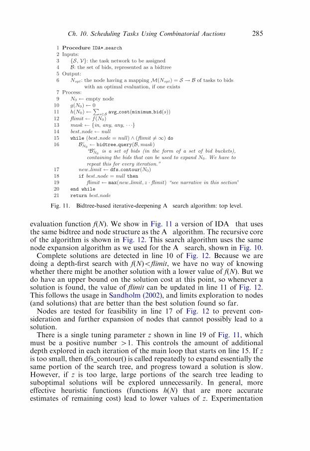
evaluation function f(N). We show in Fig. 11 a version of IDA� that usesthe same bidtree and node structure as the A� algorithm. The recursive coreof the algorithm is shown in Fig. 12. This search algorithm uses the samenode expansion algorithm as we used for the A� search, shown in Fig. 10.Complete solutions are detected in line 10 of Fig. 12. Because we are
doing a depth-first search with f(N)oflimit, we have no way of knowingwhether there might be another solution with a lower value of f(N). But wedo have an upper bound on the solution cost at this point, so whenever asolution is found, the value of flimit can be updated in line 11 of Fig. 12.This follows the usage in Sandholm (2002), and limits exploration to nodes(and solutions) that are better than the best solution found so far.Nodes are tested for feasibility in line 17 of Fig. 12 to prevent con-
sideration and further expansion of nodes that cannot possibly lead to asolution.There is a single tuning parameter z shown in line 19 of Fig. 11, which
must be a positive number W1. This controls the amount of additionaldepth explored in each iteration of the main loop that starts on line 15. If zis too small, then dfs_contourðÞ is called repeatedly to expand essentially thesame portion of the search tree, and progress toward a solution is slow.However, if z is too large, large portions of the search tree leading tosuboptimal solutions will be explored unnecessarily. In general, moreeffective heuristic functions (functions h(N) that are more accurateestimates of remaining cost) lead to lower values of z. Experimentation
Fig. 11. Bidtree-based iterative-deepening A� search algorithm: top level.
Ch. 10. Scheduling Tasks Using Combinatorial Auctions 285

using the heuristic shown in Eq. (4) shows that a good value is z ¼ 1.15, andthat it is only moderately sensitive (performance falls off noticeably withzo1.1 or zW1.2).
4 Related work
This work draws from several fields. In Computer Science, it is related towork in artificial intelligence and autonomous agents. In Economics, itdraws from auction theory and expected-utility theory. From OperationsResearch, we draw from work in combinatorial optimization.
4.1 Multi-agent negotiation
MAGNET proposes using an auction paradigm to support problem-solving interactions among autonomous, self-interested, heterogeneousagents. Several other approaches to multi-agent problem-solving have beenproposed. Some of them use a ‘‘market’’ abstraction, and some do not.Rosenschein and Zlotkin (1994) show how the behavior of agents can be
influenced by the set of rules system designers choose for their agents’environment. In their study the agents are homogeneous and there are noside payments. In other words, the goal is to share the work, in a more or
Fig. 12. Bidtree-based iterative-deepening A� search algorithm: depth-first contour.
J. Collins and M. Gini286

less ‘‘equitable’’ fashion, but not to have agents pay other agents for work.They also assume that each agent has sufficient resources to handle all thetasks, while we assume the contrary.In Sandholm’s TRACONET system (Sandholm, 1996; Sandholm and
Lesser, 1995), agents redistribute work among themselves using acontracting mechanism. Sandholm considers agreements involving explicitpayments, but he also assumes that the agents are homogeneous—they haveequivalent capabilities, and any agent can handle any task. MAGNETagents are heterogeneous, and in general do not have the resources orcapabilities to carry out the tasks necessary to meet their own goals withoutassistance from others.Both Pollack’s DIPART system (Pollack, 1996) and the Multiagent
Planning architecture (MPA) (Wilkins and Myers, 1998) assume multipleagents that operate independently. However, in both of those systems theagents are explicitly cooperative, and all work toward the achievement of ashared goal. MAGNET agents are trying to achieve their own goals and tomaximize their own profits; there is no global or shared goal.
4.1.1 Solving problems using markets and auctionsMAGNET uses an auction-based negotiation style because auctions have
the right economic and motivational properties to support ‘‘reasonable’’resource allocations among heterogeneous, self-interested agents. However,MAGNET uses the auction approach not only to allocate resources, butalso to solve constrained scheduling problems.A set of auction-based protocols for decentralized resource-allocation
and scheduling problems is proposed in Wellman et al. (2001). The analysisassumes that the items in the market are individual discrete time slotsfor a single resource, although there is a brief analysis of the use of thegeneralized Vickrey auctions (Varian and MacKie-Mason, 1995) to allowfor combinatorial bidding. A combinatorial-auction mechanism fordynamic creation of supply chains was proposed and analyzed in Walshet al. (2000). This system deals with the constraints that are representedby a multi-level supply-chain graph, but does not deal with temporal andprecedence constraints among tasks. MAGNET agents must deal withmultiple resources and continuous time, but we do not currently dealexplicitly with multi-level supply chains.5
Several proposed bidding languages for combinatorial auctions allowbidders to express constraints, for example, Boutilier and Hoos (2001) andNisan (2000b). However, these approaches only allow bidders to commu-nicate constraints to the bid-taker (suppliers to the customer, in theMAGNET scenario), while MAGNET needs to communicate constraintsin both directions.
5Individual MAGNET agents can deal with multi-level supply chains by subcontracting, but thisrequires that the initial time allocation provide sufficient slack for the extra negotiation cycles.
Ch. 10. Scheduling Tasks Using Combinatorial Auctions 287
4.1.2 Infrastructure support for negotiationMarkets play an essential role in the economy (Bakos, 1998), and market-
based architectures are a popular choice for multiple agents (see, forinstance, Chavez and Maes, 1996; Rodriguez et al., 1997; Sycara andPannu, 1998; Wellman and Wurman, 1998, and our own MAGMAarchitecture Tsvetovatyy et al., 1997). Most market architectures limitthe interactions of agents to manual negotiations, direct agent-to-agentnegotiation (Faratin et al., 1997; Sandholm, 1996), or some form of auction(Wurman et al., 1998). The Michigan Internet AuctionBot (Wurman et al.,1998) is a very interesting system, in that it is highly configurable, ableto handle a wide variety of auction rules. It is the basis for the ongoingTrading Agent Competition (Collins et al., 2004), which has stimulatedinteresting research on bidding behavior in autonomous agents, such asStone et al. (2002).Matchmaking, the process of making connections among agents
that request services and agents that provide services, will be an impo-rtant issue in a large community of MAGNET agents. The process isusually done using one or more intermediaries, called middle-agents (Sycaraet al., 1997, 1999) present a language that can be used by agentsto describe their capabilities and algorithms to use it for matchingagents over the Web. Our system casts the market in the role of match-maker.The MAGNET market infrastructure depends on an ontology to describe
services that can be traded and the terms of discourse among agents. Therehas been considerable attention to development of detailed ontologies fordescribing business and industrial domains (Fox, 1996; Gruninger and Fox,1994; Schlenoff et al., 1998).
4.2 Combinatorial auctions
Determining the winners of a combinatorial auction (McAfee andMcMillan, 1987) is an NP-complete problem, equivalent to the weightedbin-packing problem. A good overview of the problem and approaches tosolving it is explained in de Vries and Vohra (2001). Dynamic programming(Rothkopf et al., 1998) works well for small sets of bids, but it does notscale well, and it imposes significant restrictions on the bids. Sandholm(2002) and Sandholm and Suri (2003) relaxes some of the restrictions andpresents an algorithm for optimal selection of combinatorial bids, but hisbids specify only a price and a set of items. Hoos and Boutilier (2000)describe a stochastic local search approach to solving combinatorialauctions, and characterize its performance with a focus on time-limitedsituations. A key element of their approach involves ranking bids accordingto expected revenue; it is very hard to see how this could be adapted to theMAGNET domain with temporal and precedence constraints, and without
J. Collins and M. Gini288
free disposal.6 Andersson et al. (2000) describe an Integer Programmingapproach to the winner-determination problem in combinatorial auctions.Nisan (2000b) extends this model to handle richer bidding languages forcombinatorial auctions, and we have extended it to handle the MAGNETsituation in Collins and Gini (2001). More recently, Sandholm (Sandholmand Suri, 2003) has described an improved winner-determination algorithmcalled BOB that uses a combination of linear programming and branch-and-bound techniques. It is not clear how this technique could be extendedto deal with the temporal constraints in the MAGNET problem, althoughthe bid-graph structure may be of value.One of the problems with combinatorial auctions is that they are nearly
always run in a single round sealed-bid format, and this is the formatMAGNET uses. Parkes and Ungar (2000) have shown how to organizemultiple-round combinatorial auctions. Another problem is that theindividual items in a combinatorial auction are individual items; there isno notion of quantity. MAGNET will eventually need to address this. Thislimitation is overcome in Leyton-Brown et al. (2000) for simple itemswithout side constraints. The addition of precedence constraints wouldseriously complicate their procedure, and it has not yet been attempted.
4.3 Deliberation scheduling
The principal reason we are interested in search performance is becausethe search is embedded in a real-time negotiation scenario, and time mustbe allocated to it before bids are received, and therefore before the exactdimensions of the problem are known. In Greenwald and Dean (1995),deliberation scheduling is done with the aid of anytime and contractalgorithms, and performance profiles. An anytime algorithm is one thatproduces a continuously improving result given additional time, and acontract algorithm is one that produces a result of a given quality level ina given amount of time, but may not improve given additional time. Thebest winner-determination algorithms we know of for the MAGNETproblem have marginal anytime characteristics, and we know of noapplicable contract-type algorithms. In fact, Sandholm (2002) presents aninapproximability result for the winner-determination problem, leading usto believe that there may not be an acceptable contract algorithm.One way to think about deliberation scheduling is to assign the time
required for deliberation a cost, and then to balance the cost of deliberationagainst the expected benefit to be gained by the results of the deliberation.This is the approach taken in Boddy and Dean (1994). However, much ofthis analysis assumes that there is a ‘‘default’’ action or state that can be
6Under the ‘‘free disposal’’ assumption, the goal is to maximize revenue even if this means failing toallocate all the items at auction.
Ch. 10. Scheduling Tasks Using Combinatorial Auctions 289
used or attained without spending the deliberation effort, and that thereis a clear relationship between the time spent in deliberation and thequantifiable quality of the result. In the MAGNET case, the alternative todeliberation is to do nothing.
5 Conclusions
We have examined the problem of rational economic agents who mustnegotiate among themselves in a market environment in order to acquirethe resources needed to accomplish their goals. We are interested in agentsthat are self-interested and heterogeneous, and we assume that a plan toachieve an agent’s goal may be described in the form of a task network,containing task descriptions, precedence relationships among tasks, andtime limits for individual tasks. Negotiation among agents is carried outby holding combinatorial reverse auctions in a marketplace, in which acustomer agent offers a task network in the form of a RFQ. Supplier agentsmay then place bids on portions of the task network, each bid specifying thetasks they are interested in undertaking, durations and time limits for thosetasks, and a price for the bid as a whole. The presence of temporal andprecedence constraints among the items at auction requires extensions tothe standard winner-determination procedures for combinatorial auctions,and the use of the enhanced winner-determination procedure within thecontext of a real-time negotiation requires us to be able to predict itsruntime when planning the negotiation process.There are a number of real-world business scenarios where such a
capability would be of value. These include flexible manufacturing, masscustomization, travel arrangement, logistics and international shipping,health care resource management, and large-scale systems management.Each of these areas is characterized by limited capabilities and suboptimalperformance, due at least in part to the limits imposed by human problem-solving capabilities. In each of these areas, a general ability to coordinateplans among multiple independent suppliers would be of benefit, butdoes not exist or is not used effectively because of an inability to solve theresulting combinatorial problems. The use of extended combinatorialauctions such as we propose is one approach to solving these problems.There are many difficulties yet to be overcome before this vision can berealized, however, not the least of which is that such auction-based marketswould not be effective without wide adoption of new technology across anindustry, and a willingness to delegate at least some level of autonomy andauthority to that new technology.We have designed and implemented a testbed, which we call MAGNET
for multi-agent negotiation testbed, to begin exploring and testing thisvision. It includes a customer agent, a rudimentary market infrastructure,and a simple simulation of a population of supplier agents. The customer
J. Collins and M. Gini290

agent implementation is designed so that virtually all behaviors can bespecified and implemented in terms of responses to events. Events can beexternal occurrences, internal state changes, or the arrival of a particularpoint in time. The MAGNET software package is available to the researchcommunity under an open-source license.When a goal arises, the agent and its principal must develop a plan, in the
form of a task network. Once a plan is available, a bid-process plan must bedeveloped to guide the negotiation process. The bid-process plan specifieswhich tasks are to be offered in which markets, allocates time to the biddingprocess and to the plan execution, and may split the bidding into phases inorder to mitigate risk. For each bidding step in the bid-process plan, timemust be allocated to the customer to compose its RFQ, to the supplier tocompose bids, and to the customer to evaluate bids. For each auctionepisode specified in the bid-process plan, a RFQ must be composed. TheRFQ specifies a subset of tasks in the task network, and for each task, itspecifies a time window within which that task must be accomplished. Thesetting of time windows is critical, because it influences the likelihood thatbidders will bid, the prices bidders are likely to charge, and the difficulty ofthe resulting winner-determination process. If the time windows specified inthe RFQ allow task precedence relationships to be violated, then thewinner-determination process will need to choose a set of bids that can becomposed into a feasible schedule. Once the RFQ has been issued and bidsreceived, the agent must determine winners. We have described an optimalalgorithm for determining winners based on an IDA� framework.Much work remains to be done before the vision of the MAGNET
project is fully realized. Some of that work, particularly with respect to thesupplier agent and its decision processes, is already under way by othermembers of the team.With respect to the customer agent, many of the decision processes
outlined in Section 2 still need to be worked out and tested. The presentwork has resulted in models for the auction winner-determination problemand the time that must be allocated to it. For the remainder of the decisions,we need models that will maximize the expected utility of the agent or itsprincipal. These include composing the plan, developing the bid-processplan, allocating time to the deliberation processes of the customer andsuppliers, balancing negotiation time against plan execution time, settingthe time windows in the RFQ, scheduling the work in preparation forawarding bids, and dealing with unexpected events during plan execution.Babanov et al. (2003) have addressed the problem of setting time windowsin the customer’s RFQ.The language we currently use for plans and bids treats tasks as simple
atomic objects, without attributes. There are many real-world problems inwhich attributes are important, both for specifying tasks and for expressingoffers in bids. Examples include colors, quantities, dimensions, and qualityattributes. In addition, many real-world operations operate on a ‘‘flow’’
Ch. 10. Scheduling Tasks Using Combinatorial Auctions 291

basis. This includes the wine-making example we used in Chapter 2, in whichthe precedence between filling bottles and applying labels would normally beapplied bottle-by-bottle, and not at the batch level. In addition, theexpressivity of our bidding language is limited. A number of proposals havebeen made for more expressive bidding languages in combinatorial auctions(Boutilier and Hoos, 2001; Nisan, 2000b). Bidding can also be done withoracles, which are functions passed from bidder to customer that can beevaluated to produce bid conditions. Some features of a more expressivebidding language would likely have minimal impact on the winner-determination process (parameterized quality values, for example), whileothers, including the use of oracles, could require wholesale re-invention.
References
Andersson, A., M., Tenhunen, F. Ygge (2000). Integer programming for combinatorial auction winner
determination, in: Proceedings of 4th International Conference on Multi-Agent Systems, Boston, MA,
pp. 39–46.
Babanov, A., J. Collins, M. Gini (2003). Asking the right question: risk and expectation in multi-agent
contracting. Artificial Intelligence for Engineering Design, Analysis and Manufacturing 17, 173–186.
Bakos, Y. (1998). The emerging role of electronic marketplaces on the Internet. Communications of the
ACM 41, 33–42.
Boddy, M., T. Dean (1994). Decision-theoretic deliberation scheduling for problem solving in time-
constrained environments. Artificial Intelligence 67, 245–286.
Boutilier, C., H.H. Hoos (2001) Bidding languages for combinatorial auctions, in: Proceedings of the
17th Joint Conference on Artificial Intelligence, Seattle, WA, pp. 1211–1217.
Collins, J. (2002). Solving combinatorial auctions with temporal constraints in economic agents. PhD
thesis, University of Minnesota, Minneapolis, MN.
Collins, J., R. Arunachalam, N. Sadeh, J. Ericsson, N. Finne, S. Janson (2004). The supply chain
management game for the 2005 trading agent competition. Technical Report CMU-ISRI-04-139,
Carnegie Mellon University, Pittsburgh, PA.
Collins, J., C. Bilot, M. Gini, B. Mobasher (2000). Mixed-initiative decision support in agent-based
automated contracting, in: Proceedings of the Fourth International Conference on Autonomous Agents,
Barcelona, Catalonia, Spain, pp. 247–254.
Collins, J., C. Bilot, M. Gini, B. Mobasher (2001). Decision processes in agent-based automated
contracting. IEEE Internet Computing 5, 61–72.
Collins, J., G. Demir, M. Gini (2002). Bidtree ordering in IDA� combinatorial auction winner-
determination with side constraints, in: J. Padget, O. Shehory, D. Parkes, N. Sadeh, W. Walsh (eds.),
Agent Mediated Electronic Commerce IV, Vol. LNAI2531. Springer-Verlag, Berlin, pp. 17–33.
Collins, J., M. Gini (2001). An integer programming formulation of the bid evaluation problem for
coordinated tasks, in: B. Dietrich, R.V. Vohra (eds.), Mathematics of the Internet: E-Auction
and Markets. Volume 127: IMA Volumes in Mathematics and its Applications. Springer-Verlag,
New York, pp. 59–74.
Collins, J., S. Jamison, M. Gini, B. Mobasher (1997). Temporal strategies in a multi-agent contracting
protocol, in: AAAI-97 Workshop on AI in Electronic Commerce. Providence, RI.
Collins, J., M. Tsvetovat, B. Mobasher, M., Gini (1998). MAGNET: A multi-agent contracting system
for plan execution, in: Proceedings of SIGMAN, AAAI Press, Menlo Park, CA, pp. 63–68.
Chavez, A., P. Maes (1996). Kasbah An agent marketplace for buying and selling goods, in: Proceedings
of the First International Conference on the Practical Application of Intelligent Agents and Multi-Agent
Technology, London, UK, Practical Application Company, pp. 75–90.
J. Collins and M. Gini292

de Vries, S., R. Vohra (2001). Combinatorial auctions: a survey. Technical report, Tech-nische
Universitat Munchen, Munich.
Faratin, P., C. Sierra, N.R. Jennings (1997). Negotiation decision functions for autonomous agents.
International Journal of Robotics and Autonomous Systems 24, 159–182.
Fox, M.S. (1996). An organization ontology for enterprise modeling: preliminary concepts. Computers
in Industry 19, 123–134.
Greenwald, L., T. Dean (1995). Anticipating computational demands when solving time-critical
decision-making problems, in: K. Goldberg, D. Halperin, J. Latombe, R. Wilson (eds.),
The Algorithmic Foundations of Robotics. A. K. Peters, Boston, MA.
Gruninger, M., M.S. Fox (1994). An activity ontology for enterprise modelling, in: Workshop on
Enabling Technologies-Infrastructures for Collaborative Enterprises, West Virginia University.
Hillier, F.S., G.J. Lieberman (1990). Introduction to Operations Research. McGraw-Hill, New York.
Hoos, H.H., C. Boutilier (2000). Solving combinatorial auctions using stochastic local search, in:
Proceedings of the Seventeen National Conference on Artificial Intelligence, Austin, TX, pp. 22–29.
Korf, R.E. (1985). Depth-first iterative deepening: an optimal admissible tree search. Artificial
Intelligence 27, 97–109.
Leyton-Brown, K., Y. Shoham, M. Tennenholtz (2000). An algorithm for multi-unit combinatorial
auctions, in: Proceedings of the Seventeenth National Conference on Artificial Intelligence, Austin,
Texas.
McAfee, R., P.J. McMillan (1987). Auctions and bidding. Journal of Economic Literature 25,
699–738.
Nisan, N. (2000a). Bidding and allocation in combinatorial auctions. Technical report, Institute of
Computer Science, Hebrew University, Jerusalem.
Nisan, N. (2000b). Bidding and allocation in combinatorial auctions, in: Proceedings of ACM
Conference on Electronic Commerce (EC’00), Minneapolis, MN, ACM SIGecom, ACM Press,
pp. 1–12.
Parkes, D.C., L.H. Ungar (2000). Iterative combinatorial auctions: theory and practice, in: Proceedings
of the Seventeenth National Conference on Artificial Intelligence, Austin, TX, pp. 74–81.
Parkes, D.C., L.H. Ungar (2001). An auction-based method for decentralized train scheduling, in:
Proceedings of the Fifth International Conference on Autonomous Agents, Montreal, Quebec, ACM
Press, pp. 43–50.
Pollack, M.E. (1996). Planning in dynamic environments: the DIPART system, in: A. Tate (ed.),
Advanced Planning Technology. AAAI Press, Menlo Park, CA.
Rodriguez, J.A., P. Noriega, C. Sierra, J. Padget (1997). FM96.5-A Java-based electronic auction house,
in: Second International Conf on The Practical Application of Intelligent Agents and Multi-Agent
Technology (PAAM’97), London, pp. 207–224.
Rosenschein, J.S., G. Zlotkin (1994). Rules of Encounter. MIT Press, Cambridge, MA.
Rothkopf, M.H., A. Pekec, R.M. Harstad (1998). Computationally manageable combinatorial auctions.
Management Science 44, 1131–1147.
Russell, S.J., P. Norvig (1995). Artificial Intelligence: A Modern Approach. Prentice-Hall, Upper Saddle
River, NJ.
Sandholm, T. (1999). An algorithm for winner determination in combinatorial auctions, in: Proceedings
of the 16th Joint Conference on Artificial Intelligence, Orlando, FL, pp. 524–547.
Sandholm, T. (2002). Algorithm for optimal winner determination in combinatorial auctions. Artificial
Intelligence 135, 1–54.
Sandholm, T.W. (1996). Negotiation among self-interested computationally limited agents. PhD thesis,
Department of Computer Science, University of Massachusetts at Amherst, Amherst, MA.
Sandholm, T.W., V. Lesser (1995). On automated contracting in multi-enterprise manufacturing, in:
Distributed Enterprise: Advanced Systems and Tools, Edinburgh, Scotland, pp. 33–42.
Sandholm, T., S. Suri (2003). Bob: improved winner determination in combinatorial auctions and
generalizations. Artificial Intelligence 145, 33–58.
Schlenoff, C., R. Ivester, A. Knutilla (1998). A robust process ontology for manufacturing systems
integration. National Institute of Standards and Technology.
Ch. 10. Scheduling Tasks Using Combinatorial Auctions 293

Stone, P., R.E. Schnapire, M.L.L.J.A. Csirik, D. McAllester (2002). ATTac-2001: A learning, auto-
nomous bidding agent. in: Lecture Notes in Computer Science; Revised Papers from the Workshop on
Agent Mediated Electronic Commerce IV, Designing Mechanisms and Systems Table of Contents,
Springer-Verlag, London, UK, Vol. 2531, pp. 143–160.
Sycara, K., K. Decker, M. Williamson (1997). Middle-agents for the Internet, in: Proceedings of the 15th
Joint Conference on Artificial Intelligence, Providence, RI, pp. 578–583.
Sycara, K., M. Klusch, S. Widoff, J. Lu (1999). Dynamic service matchmaking among agents in open
information environments. SIGMOD Record (ACM Special Interests Group on Management of
Data) 28, 47–53.
Sycara, K., A.S. Pannu (1998). The RETSINA multiagent system: towards integrating planning,
execution, and information gathering, in: Proceedings of the Second International Conference on
Autonomous Agents, pp. 350–351.
Tsvetovatyy, M., M. Gini, B. Mobasher, Z. Wieckowski (1997). MAGMA: an agent-based virtual
market for electronic commerce. Journal of Applied Artificial Intelligence 11, 501–524.
Varian, H.R., J.K. MacKie-Mason (1995). Generalized vickrey auctions. Technical report, University of
Michigan, Ann Arbor, MI.
Walsh, W.E., M. Wellman, F. Ygge (2000). Combinatorial auctions for supply chain formation, in:
Proceedings of ACM Conference on Electronic Commerce (EC’00), Minneapolis, MN, pp. 260– 269.
Wellman, M.P., W.E. Walsh, P.R. Wurman, J.K. MacKie-Mason (2001). Auction protocols for
decentralized scheduling. Games and Economic Behavior 35, 271–303.
Wellman, M.P., P.R. Wurman (1998). Market-aware agents for a multiagent world. Robotics and
Autonomous Systems 24, 115–125.
Wilkins, D.E., K.L. Myers (1998). A multiagent planning architecture, in: Proceedings of International
Conference on AI Planning Systems, Pittsburgh, PA, pp. 154–162.
Wurman, P.R., M.P. Wellman, W.E. Walsh (1998). The Michigan Internet AuctionBot: a configurable
auction server for human and software agents, in: Second International Conference on Autonomous
Agents, Minneapolis, MN, pp. 301–308.
J. Collins and M. Gini294

Part III
Supporting Knowledge
Enterprise

This page intentionally left blank

Adomavicius & Gupta, Eds., Handbooks in Information Systems, Vol. 3
Copyright r 2009 by Emerald Group Publishing Limited
Chapter 11
Structuring Knowledge Bases Using Metagraphs
Amit BasuEdwin L Cox School of Business, Southern Methodist University, Dallas, TX 75275, USA
Robert BlanningOwen Graduate School of Management, Vanderbilt University, Nashville, TN 37203, USA
Abstract
Knowledge bases may contain a variety of knowledge types, such as datarelations, decision models, production rules, and models of workflowsystems. A graphical structure, called metagraphs, provides a single approachto structuring these information types and the interactions between them.Metagraphs may be used both for visualization and for formal algebraicanalysis. We present an overview of metagraphs and describe their applica-tion to the structuring of knowledge bases.
1 Introduction
It has been suggested that knowledge bases will be to the twenty-firstcentury what databases were to the twentieth century. Each captures thetype of information that can be stored (in machine readable form) andprocessed (in algorithmic form) at the time of their rise to prominence. Toput it another way, the twentieth century can be viewed as the age of data,and the twenty-first century can be viewed as the age of knowledge.Knowledge bases differ from databases not in the sense that knowledge
and data are mutually exclusive, but rather because the concept ofknowledge extends that of stored data relations to include additional typesof information. Another type of information is decision models, such assimulation or optimization models. A third type of information foundin knowledge bases is the collection of knowledge-based informationstructures found in artificial intelligence. This may include production rules,
297

semantic nets, and frames, but we will focus on the first of these—production rules. Yet another information type found in knowledge bases isworkflow systems. This is of special interest because an important type oforganizational knowledge is an explicit representation of the organization’sinformation processes.Each of these four types of information (i.e., stored data, decision models,
production rules, and workflow systems) can be described separately bymeans of certain graphical structures, such as entity relationship diagrams,program flowcharts, semantic nets, and data flow diagrams. However,there are two problems with these graphical representations. First, theyare primarily diagrammatic and not analytical. That is, they illustrateinformational relationships, but they do not tell us how to apply theseillustrations to construct inference paths. Second, they do not suggest howthese different information types can be integrated.In this chapter, we show how a mathematical structure called metagraphs
can be used to describe these four different types of information, the waysin which they are processed, and the ways in which they interact. Thus,metagraphs can be used as a basis for a uniform and comprehensiveanalytical framework for structuring knowledge bases. In the followingsection, we describe the four types of information found in knowledgebases—stored data, decision models, production rules, and workflowstructures. In Section 3, we present the fundamentals of metagraphs, withan emphasis on the algebraic properties of metagraphs and the use of theseproperties in constructing inference paths. In Section 4, we explain andillustrate how metagraphs can be applied to the four information typesand investigate metagraph transformations. For example, we show thatmetagraphs can be used to determine connectivity, and therefore inferencepaths, between sets of elements. They can also be used to combine data,models, rules, and workflows into a single information systems model.In addition, they can be used to project a complex system into a moresimple representation without omitting details that are important to theuser. Then in the final section, we summarize other work that has been donein this area and we identify promising topics for further research.
2 The components of organizational knowledge
We now describe the four components of organizational knowledgementioned above—stored data, decision models, production rules, andworkflow structures. The first type of information, stored data, is typicallystructured in the form of files (or data relations) in which each record is acollection of attributes describing a real-world entity. The key attributesuniquely identify the record, and therefore the entity, and the remainingcontent attributes describe other features of the entity. A graphicalstructure defining a database is the entity-relationship diagram, in which
A. Basu and R. Blanning298
the relations and the relationships between them are representeddiagrammatically. For example, a university database may contain studentand course relations, along with a relationship linking students with thecourses they are taking. Any information common to a combination (orintersection) of both student and course, such as a grade, appears in therelationship. The relationship suggests access paths that can be used toconstruct a class list or a transcript.Models are structurally similar to data, but the information they provide
does not appear in stored form. Rather, it is calculated as needed by astored algorithm which represents a real-world computational process.Instead of key and content attributes, there are input and output variables.The access paths are relationships between the outputs of some models andthe inputs of other models. For example, the output of a forecasting modelmay be the input to a production scheduling or inventory control model.Rules are if-then structures defined over logical (or yes/no) propositions.
The ‘‘if ’’ part, called the antecedent of the rule, is a conjunction ofpropositions. The ‘‘then’’ part, also a conjunction of propositions, is calledthe consequent. Access paths occur when rules are linked—that is, whenthe consequents of some rules are among the antecedents of other rules.Rules may be causal rules defined by objective considerations or they maybe elicited from experienced and knowledgeable specialists during theconstruction of expert systems. In the latter case, the rules are often calledproductions or production rules, because the antecedents are said toproduce the consequents.To understand workflows, one must first understand processes. A process
is a collection of tasks intended to achieve some desirable organizationaloutcome. From an information processing standpoint, a useful representa-tion of a process is as a network of tasks each of which transformsinput documents into output documents. An example is a loan evaluationprocess, in which the documents are loan applications, credit reports, etc.and the tasks are the preparation of these documents. Workflows areinstantiations of business processes, where the paths taken by thedocuments depend on the content of the documents. For example, thepath taken by a loan application may depend on certain documentsperformed by a risk evaluation department. In this case a single process,loan evaluation, may be instantiated into two workflows, one correspond-ing to high-risk loans and the other to low-risk loans. Knowledge ofworkflows is important because an important component of organizationalknowledge is an understanding of how the organization processes informa-tion and makes decisions in response to opportunities and problems.We have briefly described four types of information found in knowledge
bases. We have also seen that there are certain similarities between thesedifferent information types. Specifically, they are networks of informationelements (stored data, model variables, logical assertions, and documents)and relationships (data relations, decision models, production rules, and
Ch. 11. Structuring Knowledge Bases Using Metagraphs 299

workstations performing information processing tasks). This suggests thatgraph theory would be useful in analyzing the structure and processing ofthese information types. However, traditional graph theory presents certainchallenges in performing such an analysis. We will present an enhancedtheory, the theory of metagraphs, which responds to these challenges andallows us to structure and integrate knowledge bases regardless of the typeof information they contain.We should point out that there is also an alternative, but less structured,
view of knowledge bases. In this case a knowledge base is a repository ofmemos, reports, descriptions of best practices, suggestions as to who shouldbe contacted or what should be done if an unusual event occurs, etc. We donot doubt the importance of this type of information, but we will focus onthe more structured types of information found in knowledge bases. As wegain a better understanding of the modeling of this type of knowledge, weexpect that more and less structured knowledge will become explicit andwill be amenable to formal modeling techniques of the type described here.
3 Metagraphs and metapaths
A metagraph combines the properties of a directed graph (digraph) anda hypergraph. All three are based on a set of indivisible elements, whichin the case of metagraphs is called a ‘‘generating set.’’ The generatingset is supplemented with a set of relationships among the elements in thegenerating set.In the case of digraphs, the relationships are a set of ordered pairs of
elements, resulting in a network connecting certain of the elements. Theelements are often represented by points in the plane, and the ordered pairsare represented by arrows (or arcs) connecting selected pairs of points(or nodes). An example is a PERT/CPM project network, in which theelements are events that take place at instances in time and the orderedpairs are activities that span durations in time between a start event and anend event. Another example is a transportation network, in which nodes areorigins or destinations of shipments and the arcs are the shipments.However, digraphs do not properly describe the case in which a set of
source elements (e.g., the key in a relation or the input to a model) arecollectively connected to a set of target elements (e.g., the content of arelation or the output of a model). It would be possible to link each inputelement to each output element, but this would not disclose the fact thatthe entire set of source elements is needed to determine the target. Similarly,it would not be adequate to define new vertices corresponding to setsof vertices, since the element-to-element mappings in digraphs would notcapture the set-to-set mappings found in data relations, models, rules, andworkflows.
A. Basu and R. Blanning300

In the case of hypergraphs, there is no directionality. A hypergraphconsists of the generating set and a set of edges (or hyper-edges), eachof which is a subset of the generating set. Hypergraphs overcome adisadvantage of digraphs, which do not capture relationships among morethan two elements. A hyper-edge can include any number of elements, up tothe size of the generating set. In fact, some hypergraph definitions requirethat each hyper-edge contain more than two elements and that each elementin the generating set appear in at least one hyper-edge. Although the lackof directionality does pose a problem in systems modeling, the principalpurpose of hypergraphs is to facilitate combinatorial analyses.Metagraphs combine the beneficial properties of digraphs with those of
hypergraphs. A metagraph consists of a generating set and a set of orderedpairs of subsets of the generating set. Each such ordered pair is called anedge; the first subset is the invertex of the edge and the second subset is theoutvertex. We require that for each edge either the invertex or the outvertex(or both) be non-null. If the invertex is null, then the edge asserts theoutvertex, and if the outvertex is null, then the edge (in a rule-based system)asserts that the invertex is false.We note that metagraphs are similar to a hypergraph construct called
‘‘directed hypergraphs,’’ but directed hypergraphs have been explored in thecontext of individual elements as connected by their set-oriented properties.As we will see, metagraphs place more emphasis on the connectivity of setsof elements.
3.1 Metagraph definition
We now present a formal definition of metagraphs. The definitionspresented here and the theorems alluded to here are found in previousarticles and papers referenced at the end of this chapter.
Definition 1. Given a finite generating set, X ¼ {xi, i ¼ 1 . . . I }, consist-ing of elements xi, a metagraph is an ordered pair S ¼ /X, ES, in whichE ¼ {ek, k ¼ 1 . . . K} is a set of edges and each edge is a set of orderedpairs ek ¼ /Vk, WkS, with VkDX, WkDX, and Vk,Wk 6¼ ø ’k. Inaddition, if for some ek we have xiAVk and xjAWk, then the coinput of xiin ek is Vkn{xi} and the cooutput of xj in ek is Wkn{xj}.
In other words, for any edge e and any element x, the coinput of xconsists of all elements in the invertex of e other than x, and the cooutput ofx consists of all elements in the outvertex of e other than x. We note that indirected graphs all coinputs and cooutputs are null, since the edges of adirected graph are element-to-element mappings, rather than set-to-setmappings.The application of the metagraph definition to knowledge bases follows
from the definition of metagraphs (and specifically, of elements and edges)
Ch. 11. Structuring Knowledge Bases Using Metagraphs 301
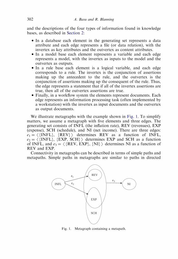
and the descriptions of the four types of information found in knowledgebases, as described in Section 2:
� In a database each element in the generating set represents a dataattribute and each edge represents a file (or data relation), with theinvertex as key attributes and the outvertex as content attributes.� In a model base each element represents a variable and each edgerepresents a model, with the invertex as inputs to the model and theoutvertex as outputs.� In a rule base each element is a logical variable, and each edgecorresponds to a rule. The invertex is the conjunction of assertionsmaking up the antecedent to the rule, and the outvertex is theconjunction of assertions making up the consequent of the rule. Thus,the edge represents a statement that if all of the invertex assertions aretrue, then all of the outvertex assertions are true.� Finally, in a workflow system the elements represent documents. Eachedge represents an information processing task (often implemented bya workstation) with the invertex as input documents and the outvertexas output documents.
We illustrate metagraphs with the example shown in Fig. 1. To simplifymatters, we assume a metagraph with five elements and three edges. Thegenerating set consists of INFL (the inflation rate), REV (revenues), EXP(expense), SCH (schedule), and NI (net income). There are three edges:e1 ¼ /{INFL}, {REV}S determines REV as a function of INFL,e2 ¼ /{INFL}, {EXP, SCH}S determines EXP and SCH as a functionof INFL, and e3 ¼ /{REV, EXP}, {NI}S determines NI as a function ofREV and EXP.Connectivity in metagraphs can be described in terms of simple paths and
metapaths. Simple paths in metagraphs are similar to paths in directed
e1
e2
e3
EXP
SCH
REV
INFL NI
Fig. 1. Metagraph containing a metapath.
A. Basu and R. Blanning302

graphs. In metagraphs, a simple path is a sequence of edges connecting asource element to a target element, where connectivity between twosuccessive edges occurs when the outvertex of the first edge overlaps (i.e.,has a non-null intersection with) the invertex of the second edge. A formaldefinition is as follows:
Definition 2. Given a metagraph /S, ES, a source xiAX, and a targetxjAX, a simple path from xi to xj is a sequence of edges P(xi, xj) ¼/e0l, l ¼ 1 . . . LS such that (1) e0lAE ’ l, (2) xiAV 0l, (3) xjAW 0L, andW 0l \ V
0lþ1 6¼ ø for l ¼ 1 . . . L–1. The coinput of xi in P(xi, xj) is[L
i¼1
Vin[Li¼1
Wl
!nfxig
and the cooutput of xj in P(xi, xj) is[Li¼1
Wl
!nfxig
We note that /e0l, l ¼ 1 . . . LS is a sequence of edges, rather than a set ofedges.
3.2 Metapaths
The concept of a simple path describes element-to-element connectivity,but it does not describe set-to-set connectivity. To do this, we need anotherconcept—that of a metapath. Consider the metagraph shown in Fig. 1.There are two simple paths from INFL to NI. They are /e1, e3S withcoinput EXP and /e2, e3S with coinput REV. Thus, there is no simple pathfrom INFL to NI with a null coinput. Even so, INFL alone is sufficient todetermine NI. To do this we must invoke all three edges: e1, e2, and e3. Butthe set of edges {e1, e2, e3} is not a simple path; it is a set of edges, not asequence of edges. Thus, we need a more general view of connectivity thatgoes beyond simple paths. This leads us to the concept of a metapath, whichin this case is the set {e1, e2, e3}. Thus, a metapath, unlike a simple path, is aset of edges, rather than a sequence of edges. In addition, the source and/orthe target may be a set of elements, although in this example they weresingleton sets.A metapath from a source to a target is a set of edges with three
properties. First, each edge in the metapath must be on a simple path fromsome element in the source to some element in the target, and all otheredges in that simple path must also be in the metapath. Second, the set of allelements in the invertices of the edges in the metapath that are not inthe outvertex of some edge in the metapath are contained in the source.Third, the set of elements in the outvertices of all the edges in the metapath
Ch. 11. Structuring Knowledge Bases Using Metagraphs 303

contains the target, although there may be additional outvertex elementsnot in the target. The first property ensures that the metapath contain noextraneous edges, and the second and third properties ensure that thesource and the edges in the metapath are sufficient to determine the target.Thus, there is no notion of coinputs for metapaths.
Definition 3. Given a metagraph S ¼ /X, ES, a source ACX, and atarget BCX, a metapath from A to B is a set of edges M(A, B) ¼{e0l, l ¼ 1 . . . L}, such that
(1) [Li¼1V0ln[
Li¼1W
0l A
(2) B [Li¼1W0l
(3) For each l ¼ 1 . . .L there is a simple path Pl (a, b) from some aAAto some bAB, such that e0lA set(Pl (a, b))DM(A, B).
The purpose of the third condition above is to ensure that M(A, B) doesnot contain edges in simple paths from some elements in the set B to otherelements in another set C. Their inclusion would not invalidate the first twoconditions, but they also would not be needed to define a metapath fromA to B. However, as we will see in Section 4.3, the definition of anotherconcept, that of metapath dominance, will serve to identify other types ofsuperfluous elements and edges. The construction of metapaths is describedin Basu and Blanning (1994b).
3.3 Metagraph algebra
Although metagraphs can be illustrated diagrammatically, as was done inFig. 1, it is also possible to represent them algebraically. This makes itpossible to perform calculations that will identify such properties as theexistence of simple paths and metapaths, rather than to identify them byvisual inspection. The foundation of the algebraic approach is the adjacencymatrix. An adjacency matrix is a square matrix with one row and onecolumn for each element in the generating set. Each (row, column) memberAij in the adjacency matrix is a set of zero or more triples, one for each edgecontaining row element in its invertex and the column element in itsoutvertex. The first component of the triple is the coinput of the rowelement, the second component is the cooutput of the column element, andthe third component is the name of the edge, represented as a sequence.The reason that there may be no triples in a particular Aij is that there
may be no edges in the metagraph with xi in its invertex and xj in itsoutvertex. In this case, Aij would be null. The reason that there may be morethan one triple in a particular Aij is that there may be multiple edges in themetagraph with xi in its invertex and xj in its outvertex. For example, if itwere possible to calculate net income from revenue and schedule, thenthere would be an additional edge e4 ¼ /{REV, SCH}, {NI}S. In that case
A. Basu and R. Blanning304

we would have AREV,NI ¼ {/{EXP}, ø,/e3SS,/{SCH}, ø,/e4SS} andASCH,NI ¼ {/{REV}, ø, /e4SS}. We will see another example of multipletriples in the description of the A2 matrix below.The adjacency matrix of the metagraph in Fig. 1 appears in Table 1.
Twenty of the twenty-five members of the matrix do not correspond toany edges and are null. For example, there is no single edge directlyconnecting an invertex containing INFL to an outvertex containing NI,so AINFL,NI ¼ ø. However there is an edge, e3, connecting REV to NI, sothe member AREV,NI consists of the triple {/{EXP}, ø,/e3SS}; EXP is thecoinput of INFL in e3, the cooutput of NI in e3 is null, and e3 is the edge.A multiplication operation has been defined for metagraph adjacency
matrices (Basu and Blanning, 1994a), and this can be used to calculatesuccessive powers of these matrices. As with simple graphs and digraphs,the nth power of the adjacency matrix discloses all paths of length n from asource element to a destination element. The square of the adjacencymatrix, A2, consists entirely of null members, except for A2
INFL,NI ¼
{/{EXP}, {REV},/e1, e3SS,/{REV}, {EXP, SCH},/e2, e3SS}. Eachmember of this set corresponds to a simple path of length 2 betweenINFL and NI; the first is /e1, e3S and the second is /e2, e3S. All higherpowers of A consist entirely of null members, since there are no simplepaths of length greater than two in the metagraph.The powers of the adjacency matrix can be summed to produce the
closure of the adjacency matrix. In this case, the closure of A is AþA2, asillustrated in Table 2. The closure identifies all simple paths of any lengthand can be combined with the requirements of Definition 3 to find allmetapaths between any two sets of elements in the metagraph, if suchmetapaths exist. The closure can also be used to identify any cyclesin the metagraph—that is, any simple paths from an element to itself.A metagraph contains a cycle if and only if its closure has at least onenon-null member in its diagonal. The cycle will be the third component inthe triple. There will be one such triple for each element in the cycle.
Table 1
Adjacency matrix for Fig. 1
INFL REV EXP SCH NI
INFL ø {/ø, ø,
/e1SS}
{/ø, {SCH},
/e2SS}
{/ø, {EXP},
/e2SS}
ø
REV ø ø ø ø {/{EXP}, ø,
/e3SS}
EXP ø ø ø ø {/{REV}, ø,
/e3SS}
SCH ø ø ø ø ø
NI ø ø ø ø ø
Ch. 11. Structuring Knowledge Bases Using Metagraphs 305

3.4 Metapath dominance and metagraph projection
We conclude this section by addressing two issues, one related tometapaths and the second to entire metagraphs. The metapath-related issueis whether the metapath contains any elements or edges that are not neededto connect a source to a target. In other words, we wish to know whetherthe metapath contains superfluous elements or edges. This leads to theconcept of metapath dominance. The metagraph-related issue is whether ametagraph can be simplified by eliminating some of the elements and edgesin ways that retain certain specified important relationships but hideunimportant relationships. This leads to the concept of projecting ametagraph over a subset of its generating set.We begin with the concept of metapath dominance.
Definition 4. Given a metagraph S ¼ /X, ES, for any two sets ofelements BDX and CDX, (1) a metapath M(B, C) is edge dominant if noproper subset of M(B, C) is also a metapath from B to C and (2) ametapath M(B, C) is input dominant if there is no BuDB such thatM(Bu, C) is a metapath from Bu to C. A metapathM(B, C) is dominant if itis both edge dominant and input dominant.
In other words, a metapath from a set B to a set C is edge dominant if it isnot possible to remove any edges from the metapath and still have ametapath from B to C. It is input dominant if it is not possible to removeany elements from B and have a metapath from the resulting subset of B toC. It is dominant if it is both edge and input dominant. We note that thisalso applies to conditional metagraphs, since a conditional metagraph isstill a metagraph, but with an expanded generating set.We now turn to the concept of a projection. Before giving a formal
definition, we present an example. Consider the metagraph illustrated atthe top of Fig. 2. Price (PRI) determines volume (VOL), which in turn
Table 2
Closure of the adjacency matrix for Fig. 1
INFL REV EXP SCH NI
INFL ø {/ø, ø,
/e1SS}
{/ø, {SCH},
/e2SS}
{/ø, {EXP},
/e2SS}
{/{EXP}, {REV},
/ e1, e3SS,
/{REV}, {EXP, SCH},
/e2, e3SS}
REV ø ø ø ø {/{EXP}, ø,
/e3SS}
EXP ø ø ø ø {/{REV}, ø,
/e3SS}
SCH ø ø ø ø ø
NI ø ø ø ø ø
A. Basu and R. Blanning306

determines both capacity requirements (CAP) and expense (EXP), andprice and volume together determine revenue (REV). Let us say that we areinterested only in whether there is a relationship between price and expense.There are three issues here. First, although price indirectly determinesexpense, there is an intervening variable, volume, in which we are notinterested. Second, volume also determines capacity, in which we are notinterested. Third, price, along with volume, determines revenue, butrevenue is of no interest to us. A projection of the metagraph onto thesubset Xu ¼ {PRI, EXP} of the generating set, would clarify any relation-ships in Xu and not burden us with information about the remainingelements in XnXu.This projection is illustrated at the bottom of Fig. 2. We can see that price
determines expense. This relationship is determined by a new edge eu, whichis not found in the original (or base) metagraph. The projected edge eu isderived from e1 and e2 and is called a composition of these edges.The composition c(eu) ¼ {{e1, e2}} is the set of all metapaths describingrelationships involving elements of Xu. In this case, there is only one suchmetapath, {e1, e2}, but more generally there could be several metapathsconnecting PRI to EXP. Therefore, a composition is a set of sets (of edgesin the base metagraph).We are now ready for a formal definition.
Definition 5. Given a base metagraph S ¼ /X, ES and XuDX, ametagraph Su ¼ /Xu, EuS is a projection of S onto Xu if
� for any eu ¼ /Vu, WuSDEu and for any xuAWu there is a dominantmetapath M(Vu, {xu}) in S,
PRI
PRI EXP
VOL CAP
EXP
e1 e2
e3
e’
REV
Fig. 2. A metagraph and its projection.
Ch. 11. Structuring Knowledge Bases Using Metagraphs 307
� for every xuAXu, if there is any dominant metapath M(V, {xu}) in Swith VDXu, then there is an edge /Vu, WuSAEu, such that V ¼ Vuand xuAWu, and� no two edges in Eu have the same invertex.
The third condition simplifies the projection by minimizing the numberof edges in it. As a result, for any S ¼ /X, ES and any XuDX the projectionof S onto Xu exists and is unique. An algorithm for constructing projectionsis found in Basu et al. (1997) and also in Basu and Blanning (2007). Thus, aprojection provides us with a high-level view of a complex system, and acomposition tells us how the relationships in the high-level view can bederived from those in the base system.
4 Metagraphs and knowledge bases
In this section, we examine three issues. In Section 4.1, we examine theapplication of metagraphs to the four types of information contained inknowledge bases, including the case in which a single knowledge basecontains more than one type of information and the information typesinteract. For example, a rule base may constrain a model base and maydetermine how the models may interact with each other. We also addressa more specialized topic, the existence of cycles in a knowledge base andtherefore in the metagraph that models the knowledge base. Cyclesrepresent simultaneity in the relationships among the elements (e.g., there isa directed relationship from xi to xj, but there is also a directed relationshipfrom xj to xi). We will present a supply–demand example below. Theexistence of cycles may affect the knowledge base in ways that may not beimmediately apparent. Then we will examine an additional topic—thecombination of data, models, rules, and workflows in a single metagraph(Section 4.2). We conclude this section by discussing simplified views of ametagraph (Section 4.3). These are metagraphs that capture the essentialelements of a base metagraph as defined by the user and omit extraneousdetails. They are constructed using the projection operator defined above.
4.1 Applications of metagraphs to the four information types
The first of the four information types is stored data, usually in the formof data relations. Each relation is represented by a metagraph edge in whichthe invertex corresponds to the key and the outvertex corresponds to thecontent. An access path between two sets of data attributes is representedby a metapath in which the first set of attributes is the source of themetapath and the second set of attributes is the target of the metapath.We note that a projection operation in metagraphs corresponds to the
decomposition (or projection) of relational databases into a succession of
A. Basu and R. Blanning308

higher normal forms to eliminate storage anomalies. For example, considera database containing a transitive dependency (Fig. 3). Each employee(EMP) is in a single department (DEP), which in turn has a single location(LOC). Placing all of this into single relation (or metagraph edge) presentsproblems if the location of a department should change, if the last employeein a particular department should leave, or if a new department in aknown location and yet to contain any employees should be established.A better approach is to project the edge (i.e., decompose the relation) intotwo components, one involving a functional dependency between EMP andDEP, and the other involving a functional dependency between DEPand LOC.The second information type is decision models, each of which is an
edge with the input to the model represented by the invertex of the edgeand the output by the outvertex. As with data relations, access paths(for integrating the models) correspond to metapaths in the metagraph.But there is an additional issue seldom found in databases: the possibleexistence of cycles in the metagraph, corresponding to cycles in the modelbase, which in turn will correspond to cycles in the real world. These realworld cycles will arise whenever there are two (or more) variables or sets ofvariables, each of which affects the other. In other words, the relationshipsare not unidirectional, but rather are bidirectional, and this simultaneity inrelationships must be resolved.For example, consider the cyclic metagraph in Fig. 4 representing a
model base containing two models. A demand model (DMD) calculates the
EMP DEP LOC
EMP DEP
DEP LOC
Fig. 3. Transitive dependency.
Ch. 11. Structuring Knowledge Bases Using Metagraphs 309

volume (VOL) of a product that will be sold as a function of the pricecharged for the product (PRI) and the GNP of the country in which thecompany selling the product is found. A supply model (SUP) calculatesthe equilibrium price (again, PRI) at which the product will be sold andthe needed production capacity (CAP) as a function of the volume sold(again, VOL).The method of solving these relationships depends on their functional
forms. If they are simple functional relationships (e.g., linear functions),then they can be solved analytically as simultaneous equations. Unfortu-nately this is seldom the case, and it is usually necessary to solve themnumerically using an iterative convergence procedure. A value is posited foreither PRI or VOL, as well as GNP, the appropriate model is used tocalculate VOL or PRI, the other model is used to reverse the process, andthe iterative cycle continues until the process converges. There are severalproblems here: one is that the iterative process may not converge, another isthat the convergence may be too slow, and the third is that there may bemultiple equilibria. But in any case, cycles in the model base, which can bedetected by visual inspection or by the existence of non-null members inthe diagonal of the adjacency matrix, may complicate the solution of themodels.Another complicating factor is the computational effort needed to solve
the models. In part this may arise from the size and complexity of themodels themselves, but it may also result from the characteristics of themodel inputs and outputs represented by the elements in the metagraph.For example, the variables corresponding to PRI and VOL may be indexedover geographical regions, industrial sectors, and/or time stages, thuscomplicating the analysis.The third information type is production rules, in which the elements in
the generating set correspond to propositions that may be either true orfalse. For example, in Fig. 4, the edges would correspond to rules in which
DMD
SUP
VOL
GNP
PRI
CAP
Fig. 4. Cyclic metagraph.
A. Basu and R. Blanning310
the invertices and outvertices would be conjunctions of the appropriatepropositions:
DMD: GNP 4 PRI - VOLSUP: VOL - PRI 4 CAP
In an acyclic metagraph, a metapath would correspond to an inference pathin the rule base, but this need not be true in a cyclic metagraph. In thisexample, each of the two rules (DMD and SUP) correspond to (rathersimple) inference paths. For example, if we know the truth values of GNPand PRI, we can determine the truth value of VOL. However, when themetagraph is cyclic, this breaks down. Specifically, there is an inferencepath between a source and a target if and only if there is an acyclicmetapath connecting the source to the target.In the above example if we consider both rules, there is a metapath with
source {GNP} and target {PRI, VOL, CAP}. But the rule base (and hencethe metagraph) is cyclic and there is no acyclic metapath connecting thesource to the target and so the two rules are mutually inconsistent. Forexample, if GNP ¼ T, PRI ¼ F, VOL ¼ F, and CAP ¼ F, then both of therules DMD and SUP would be true. However, the implication correspond-ing to the metapath described above (i.e., GNP-PRI4VOL4CAP) wouldbe false.We should point out that in the metagraph representation of rule bases
propositions are generally assumed to be positive. That is, there is nonegation operator except in special cases. The exception is the use ofmetagraphs in discovering implicit integrity constraints in rule bases. Thisexception will not be addressed here.The fourth information type is a workflow system, in which the
generating set corresponds to documents and the edges represent work-stations that transform input documents into output documents. The issueshere are similar to those in model management, except that there is humanintervention in the transformations. That is, in an acyclic system metapathscorrespond to solution procedures (or inference rules). However, cyclicsystems require iterative processes with the attendant possibilities of (1) lackof convergence, (2) unacceptably slow convergence, and (3) multipleequilibria.
4.2 Combining data, models, rules, and workflows
There are several ways in which metagraphs can be used to combine datarelations, decision models, production rules, and workflow systems. Forexample, a data element can be an input to a model or the output of amodel can be part of the key in a data relation. The same can be said forworkflow systems—for example, data relations and workflows and fordecision models and workflows. In each of these cases, the metagraph
Ch. 11. Structuring Knowledge Bases Using Metagraphs 311

constructs described above can be integrated in a reasonably straightfor-ward manner.A more interesting case occurs when the data elements include
propositions, which can be in the invertex or outvertex of a metagraphedge. Both possibilities are illustrated in Fig. 5. Edge e1 calculates the truthvalue of a proposition p from the value of the variable PRI. For example,if PRI is the price of a product (as in the examples above) and p is theproposition ‘‘The price is less than twenty dollars’’ (i.e., ‘‘PRIo20’’), thene1 represents the calculation of the truth value of p from the numerical valueof PRI.However, when a proposition is in the invertex of an edge, the
interpretation is quite different. In this case, we are asserting that theproposition must be true for the edge to be valid—that is, for the edge to beused in a metapath. An example is the edge e2 in Fig. 5, which states thatVOL can be calculated from PRI if p is true. In other words, we can executethe model (or data relation or workstation) represented by e2, but only ifthe price is less than 20 dollars. There is no suggestion here as to whathappens if the price is greater than or equal to 20 dollars, although thiscondition can be addressed by defining another proposition, requiringanother edge. Thus, we can think of a proposition in an invertex as anassumption that must be true for the edge to be valid. In this case in orderto invoke the relation/model/workstation represented by the edge e2, wemust assume that the price is less than $20.A metagraph in which there are propositions in some of the invertices is
called a conditional metagraph. In a conditional metagraph, the generatingset is partitioned into two disjoint sets of data elements, the quantitativeand qualitative variables formerly represented by X and a set ofpropositions. The former will be denoted XV, and the latter will be denotedXP. The entire generating set will now be denoted X, so we haveX ¼ XV,XP, with XV-XP ¼ ø. In addition, we require that if an outvertexcontains a proposition in XP, then it cannot contain any variable in XV—inother words, for any eAE and pAXP, then if pAWe, we have We ¼ {p}.Now for any metapath, we can identify those assumptions that must be trueinitially for the metapath to be valid and those assumptions that must alsobe true but whose values will not be known until the appropriate edges havebeen executed.
e1 e2
VOL PRI p
Fig. 5. Conditional metagraph.
A. Basu and R. Blanning312
The concept of a conditional metagraph is of interest because it allowsone information structure to enable or disable another such structure.For example, one workflow process may generate a proposition that willactivate another workflow or that will determine the details of how thesecond workflow will be implemented. In the contest of an order entryprocess, the enabling workflows may be a credit check on a customer andan evaluation of inventory levels to determine existing inventories aresufficient to fill the order or whether additional production is needed. Theenabled process would be a process for assembling and packaging the lineitems in the order and shipping them to the customer. In a more complexsystem, another enabling process might access a database describing a partsexplosion in order to transform a demand for finished goods into deriveddemands for subassemblies and piece parts. Thus, conditional metagraphscan model a situation in which one process can turn on, turn off, or modifyanother process.
4.3 Metagraph views
It is sometimes useful in knowledge processing to provide a simplifiedview of knowledge bases. This will make it possible for managers interestedin the content of a knowledge base to examine those elements and relation-ships (edges) of greatest relevance to a particular situation. A projectionprovides that information in an explicit and convenient form.A single metagraph may have several views, as defined by the elements
over which the projection is taking place. For example, in Fig. 2, weillustrated a projection over {PRI, EXP}, which resulted in the composition{{e1, e2}}. However, someone with different interests may wish to focus onthe variables PRI and REV, which would have resulted in a projectioncontaining as its edge the composition eu ¼ {{e1, e3}}. Yet anotherpossibility is to focus on Xu ¼ {EXP, REV}, which would result in a nullprojection, since there are no metapaths connecting {EXP} with {REV}.We note that a metapath in a projection of a conditional metagraph does
not necessarily imply an inference path. The reason is if the metagraph is aconditional metagraph, a proposition not in the projection set may be false.For example, if in the example of Fig. 5, we project over Xu ¼ {PRI, VOL},then we find that {PRI} is connected to {VOL} using the compositioneu ¼ {{e1, e2}}. However we do not see in the projection that p must betrue (i.e., PRI must be less than $20) for connectivity to occur. Thus, aprojection simplifies matters while retaining underlying connectivity, but itis wise to be careful that the omitted information is really unimportant.Projection is not the only method for simplifying metagraphs. Yet
another approach is to use contexts. A context is applied to a conditionalmetagraph and it focuses on the propositions in the generating set,rather than on the variables. We will not describe contexts here, but we
Ch. 11. Structuring Knowledge Bases Using Metagraphs 313

summarize this concept in Section 5.2 where we discuss other work onmetagraphs.In summary, for large and complex metagraphs (including conditional
metagraphs) methods are available to provide simplified views withoutomitting the underlying connectivity, and this increases the usefulness ofmetagraphs.
5 Conclusion
In this section, we summarize work that we have done on metagraphs,including work not described above but that has been published elsewhere,and discuss its relevance to knowledge management. Then we suggestadditional work that might be done in this area.We began in this chapter by describing knowledge bases in terms of a
variety of information types—stored data, decision models, productionrules, and workflow systems. We then defined metagraphs as a collectionof set-to-set mappings, where the first (invertex) set represents inputs to themappings (key attributes, input variables, antecedents, and input docu-ments), and the second (outvertex) set represents outputs of the mappings(content attributes, output variables, consequents, and output documents).The set-to-set property of metagraphs allows for a rich type of connectivity,represented by metapaths, which can be applied not only to each of theinformation types taken separately, but also to systems that integrate theinformation types, leading to the concept of a conditional metagraph.We concluded with the definition of a projection, which transforms a basemetagraph into a high-level view that focuses on those elements of interestto a specific decision maker and the relationships between them.
5.1 Related work
The work we have reported here summarizes the fundamental researchthat has been done on metagraphs. But much more work has to be done aswell. We will present a brief summary, as follows:
� Hierarchical Modeling: Consider the case in which two separatemetagraphs have overlapping but not identical generating sets. Anexample is metagraphs that describe manufacturing and marketinginformation, with distribution information common to both. We haveexamined the relationship between projections of the aggregatemetagraph and projections of the individual metagraphs and havesuggested implications for information systems design and organiza-tion design (Basu et al., 1997).� Independent Submetagraphs (ISMGs): A submetagraph is simply ametagraph contained within another metagraph. A submetagraph is an
A. Basu and R. Blanning314
ISMG if there are ‘‘pure’’ input elements such that all elements inthe submetagraph are determined either by the pure elements or byother elements in the submetagraph, and there is a similar conditiondefined in reverse for a set of pure output elements. We examineconditions under which the union and intersection of ISMGs areISMGs. ISMGs are useful in determining whether a subprocess isindependent of a larger process. This would occur when the elementsin the subprocess other than the pure inputs and the pure outputs donot interact with other elements in the larger metagraph. We alsoexamine conditions under which two subprocesses contained withina larger process are mutually independent of each other (Basu andBlanning, 2003).� Attributed Metagraphs: Attributes are labels attached to edges and maybe used to specify such things as resources needed to implement themodels or workstations represented by the edges. The resourcesmay be hardware, software, or human (e.g., programmers, analysts, orother specialists). We have examined cases in which a commonresource is used by several edges and in which adjacent edges (andtherefore, successive tasks) communicate through the use of a commonresource (Basu and Blanning, 2000).� Metagraph Contexts: A context is a metagraph transformationdefined for a conditional metagraph in which each proposition is eitherknown to be true, is known to be false, or is undetermined. Some of thepropositions and edges in a context can be deleted, and therefore, acontext provides a simplified view of a metagraph. There is aninteresting relationship between contexts and projections—they arecommutative. That is, for a given conditional metagraph and a givensubset of the generating set, the context of its projection is the projectionof its context (Basu and Blanning, 1998).� Fuzzy Metagraphs: The use of metagraphs for representing rules inrule-based knowledge bases has been extended to fuzzy rules, usingfuzzy metagraphs (Tan, 2006). This approach combines the set-to-setrepresentative power of metagraphs with the expressive features offuzzy systems, and has been shown to offer some distinct advantagesfor both automated reasoning systems and in intelligent informationretrieval.
5.2 Research opportunities
Although there has been significant progress in the development andapplication of metagraphs, there is much left to be done. We now speculateon several areas that might yield fruitful results:
� A Metagraph Workbench: A software and database workbench formetagraphs would help a manager or analyst to answer such questions
Ch. 11. Structuring Knowledge Bases Using Metagraphs 315

as: (1) given a description of known information and desiredinformation, how can existing modules be used to obtain the desiredinformation, (2) what other information would be obtained as abyproduct of this process, (3) are there alternative ways of obtainingthe desired information, and (4) what new modules might be usefulin performing these analyses? The workbench would containrepositories known information and existing modules, as well assoftware for calculating metapaths, projections, and contexts, and auser interface.� Metagraph-Based Models of Social Networks: How can one usemetagraphs to model formal and informal social networks andorganization structures and the consequent channels of communica-tion? This might require the elimination of the directional characterof metagraphs to model bilateral communication networks. In otherwords, an edge would be defined as an unordered pair of subsets of thegenerating set. What are the consequences of doing this?� Metagraphs in Software Engineering: How can/should metagraphs beused in feasibility studies, system analysis, system design, and projectimplementation? Can metagraphs or metagraph-like features be usefulin enhancing data flow diagrams, entity-relationship diagrams, andproject management diagrams? Can metagraphs assist in constructingscenarios for software and system testing?
In conclusion, we believe that the topic of metagraphs offers a promisingset of opportunities to capture the inherent complexity of knowledge bases.The reason is that metagraphs are based on a worldview that describes thevariety of modules found in knowledge bases—that is, modules involvingdata, models, rules, and workflows. This worldview relies on set-to-set,rather than point-to-point, mappings, and these mappings can represent therich interactions found in knowledge bases. This will extend existingthinking about knowledge bases and may even help us in an effort tostructure currently unstructured knowledge bases.
References
Basu, A., R.W. Blanning (1994a). Metagraphs: a tool for modeling decision support systems.
Management Science 40, 1579–1600.
Basu, A., R.W. Blanning (1994b). Model integration using metagraphs. Information Systems Research
5, 195–218.
Basu, A., R.W. Blanning (1998). The analysis of assumptions in model bases using metagraphs.
Management Science 44, 982–995.
Basu, A., R.W. Blanning (2000). A formal approach to workflow analysis. Information Systems
Research 11, 17–36.
Basu, A., R.W. Blanning (2003). Synthesis and decomposition of processes in organizations. Information
Systems Research 14, 317–355.
A. Basu and R. Blanning316

Basu, A., R. W. Blanning (2007). Metagraphs and Their Applications. Edited by R. Sharda and S. Vos,
Kluwer Academic Publishers, New York, Expository and Research Monograph, Integrated Series in
Information Systems.
Basu, A., R.W. Blanning, A. Shtub (1997). Metagraphs in hierarchical modeling. Management Science
43, 623–639.
Tan, Z.-H. (2006). Fuzzy metagraph and its combination with the indexing approach in rule-based
systems. IEEE Transactions on Knowledge and Data Engineering 18, 829–841.
Ch. 11. Structuring Knowledge Bases Using Metagraphs 317

This page intentionally left blank

Adomavicius & Gupta, Eds., Handbooks in Information Systems, Vol. 3
Copyright r 2009 by Emerald Group Publishing Limited
Chapter 12
Information Systems Security and StatisticalDatabases: Preserving Confidentiality throughCamouflage
Robert Garfinkel, Ram Gopal and Manuel NunezThe University of Connecticut, Storrs, CT 06269, USA
Daniel RiceDepartment of Information Systems and Operations Management, The Sellinger School of
Business, Loyola College in Maryland, 4501 N. Charles Street, Baltimore, MD 21210, USA
Abstract
This chapter outlines some of the major themes of information systems secu-rity in statistical databases (SDB). Information security in databases, includingconfidentiality in SDBs and privacy-preserving data mining, is discussedbroadly while the chapter primary focuses on the protection of SDBs againstthe very specific threat of statistical inference. Several protection mechanismsthat researchers have developed to protect against this threat are introducedincluding data restriction, perturbation, and data-hiding techniques. Oneparticular data-hiding model, Confidentiality via Camouflage (CVC), isintroduced and demonstrated in detail. CVC provides a functional and robusttechnique to protect online and dynamic SDBs from the inference threat.Additionally, the chapter demonstrates how CVC can be linked to an econo-mic model for an intermediated electronic market for private information.
1 Introduction
Database (DB) security pertains to a database’s ability to reliably andsecurely handle sensitive information. A secure DB can protect users fromthe risk of loss, destruction, or misuse of information. DB security should bestrong enough to protect against all the above risks, but it is increasinglyimportant that it protects against the threat of an attacker who is trying to
319

gain access to sensitive information. Naturally, the requirement for strongDB security leads to an inevitable problem, namely the ‘‘conflict between theindividual’s right to privacy and the society’s need to know and processinformation’’ (Palley and Siminoff, 1987).Much of information systems (IS) security is handled at the operating
system (OS) level. For example, the modern OS is capable of concurrentlymanaging multiple processes and multiple users while ensuring that the datastored and accessed by each of these processes and users remains separated.This requires the OS to allow only authorized users to run processes forwhich they have permission and to restrict processes and users from accessingunauthorized data storage locations. Separation in the OS is implementedusing access control matrices coupled with user authentication (verifying useridentity before authorizing access). Additionally, the modern OS uses avariety of other security features to ensure information security includingfirewalls, intrusion detection, security policy implementation, routine back-ups, and data encryption.IS security is also implemented at the application level, for example,
database management systems (DBMS), such as Oracle and MicrosoftAccess, generally come equipped with many security features independentfrom the OS. DBMS level security protects against specific informationthreats that could result in the accidental or intentional loss, destruction,and misuse of data. The modern DBMS typically supports user authentica-tion, backups, data encryption, and other information security features.Protecting against data misuse is often difficult because it requires abalancing of the user’s right to access data with protection. The misuse ofdata implies that an intentional act results in the improper release ofinformation to unauthorized parties (data confidentiality), the unauthorizedor unwanted modification of data (data integrity), or the loss of dataavailability (Castana et al., 1995). In order to protect the confidentiality,integrity, and availability of data, standard DBMS security features ofteninclude some or all of the following security features:
� DB views that restrict the information the DB reveals to users.� Data integrity controls that are enforced by the DB during queries andupdates to preserve integrity.� User authentication and access controls that limit unauthorized useraccess to the DB, views, queries, and tables.� User-defined procedures that limit users ability to manipulate data inthe DB.� Encryption that limits the readability of DB data (requires access tothe decryption algorithm and a secret key in order to read data).
While OS and application level security provide a first line of defenseagainst some common DB information security threats, there remains anadditional threat, called statistical inference, that often results in the misuseof data. The statistical inference problem arises when revealed aggregate
R. Garfinkel et al.320
information on sensitive data can be combined with other information todeduce individual confidential data on records in the DB (Denning, 1980).This problem is particularly piquant in statistical databases (SDBs) whichhave been specifically tailored to handle statistical queries and in data-mining applications that often analyze massive sets of privacy-sensitive data.The goal of both SDBs, and data-mining applications, is to allow users to
query a system that returns important information from stored data. SDBsare specifically designed to answer statistical queries such as count, mean,standard deviation, minimum and maximum, and correlation queries (Date,2000). Data-mining applications, on the other hand, allow users to makesense of large data sets collected in the course of daily activities for thepurpose of knowledge discovery. While the implementation of SDB anddata-mining applications are quite different, they both may be vulnerable tostatistical inference attacks. Therefore, statistical disclosure control (SDC)and data confidentiality techniques have been developed to protect againststatistical inference in SDBs while privacy-preserving data-mining techniqueshave been developed to protect against statistical inference in data-miningapplications (Agrawal and Srikant, 2000; Willenborg and de Waal, 2001).
2 DB Concepts
A DB is a collection of logically related data and the rules that govern therelationships between the data. A relational DB consists of two-dimensionaltables storing information about real life entities and composed of records,the rows of the table, and attributes, the columns. The terms ‘‘DB’’ and‘‘relational DB’’, as well as DBMS and relational DBMS, are used inter-changeably in this chapter. Each record, or instance, contains one group ofrelated data including the attributes. Each field represents an elementary unitof the data. A typical relational DB model consists of multiple tables and theDB schema contains information about the logical structure of DB (that is,how the DB tables are related).This chapter presents an example DB table that represents a simple but
typical SDB table. The example table is used to illustrate the concept of SDBsecurity. The table stores multiple non-confidential attributes (categoricaland numeric) and a single confidential attribute (numeric). You will noticethat additional attributes (protection vectors) have been created and addedfor the sole purpose of protecting the confidential attribute.
2.1 Types of statistical databases (SDBs)
Another important concept for DB security is the intended use of the DB.Is it a stand alone version or networked throughout the world? Does thedata change over time or does it stay the same? Does the system handle
Ch. 12. Information Systems Security and Statistical Databases 321
queries as they arrive, or in a batch? Answering these questions can allow usto begin to classify DBs by their intended use environment. Turn andShapiro (1978) classify SDBs by the following system environments:
1. Online–Offline–Online SDBs are real-time, meaning the user interactswith the DB and query answers, updates, and deletions occur at thetime of the request. The user of an off-line SDB does not directlycontrol or even know when a data request is processed.
2. Static–Dynamic–Static SDBs are created once and never change duringthe lifetime of the DB (no updates or deletions). A dynamic SDB canchange over time, increasing the complexity of the DB security.
3. Centralized–Decentralized–Centralized SDBs essentially refer to asingle copy of the DB that is maintained in one location. DecentralizedSDBs, also called distributed SDBs, are multiple copy overlappingDBs that can be maintained in several locations. Decentralized SDBscomplicate security.
4. Dedicated–Shared Computer System–Dedicated SDBs exist to serve asingle application, while shared SDBs exist to serve several applicationsconcurrently. Shared SDBs increase the security risks and complexity.
System environment often impacts the complexity of the data protectionproblem, as well as performance requirements. For example, an online DBthat requires ad-hoc queries to be answered as they arrive necessitates thatthe SDB be capable of rapidly handling requests. Dynamic DBs often allowusers to add and delete data and may be more vulnerable to inferentialdisclosure risks (a user with limited read and write privileges could trackchanges to query responses before and after updating records, which canthen lead to disclosure of sensitive data). System environment can complicatethe operational and security requirements of the SDBs.
2.2 Privacy-preserving data-mining applications
Data mining, also called knowledge discovery and exploratory analysis,allows for the exploration of volumes of data collected from various sources,such as cash register data and credit card purchases, that are dumped intodata warehouses. The data are analyzed using some classical statisticalapproaches, such as regression analysis, as well as alternative data-miningapproaches including cluster analysis, neural networks, and decision treeanalysis. The recent advances in the exploratory power of data-miningalgorithms necessitates full consideration of the privacy implications of datamining. Privacy-preserving data mining is a stream of research thatinvestigates these implications. Privacy-preserving data mining often drawsfrom statistical disclosure control approaches developed for SDBs (Verykioset al., 2004).
R. Garfinkel et al.322
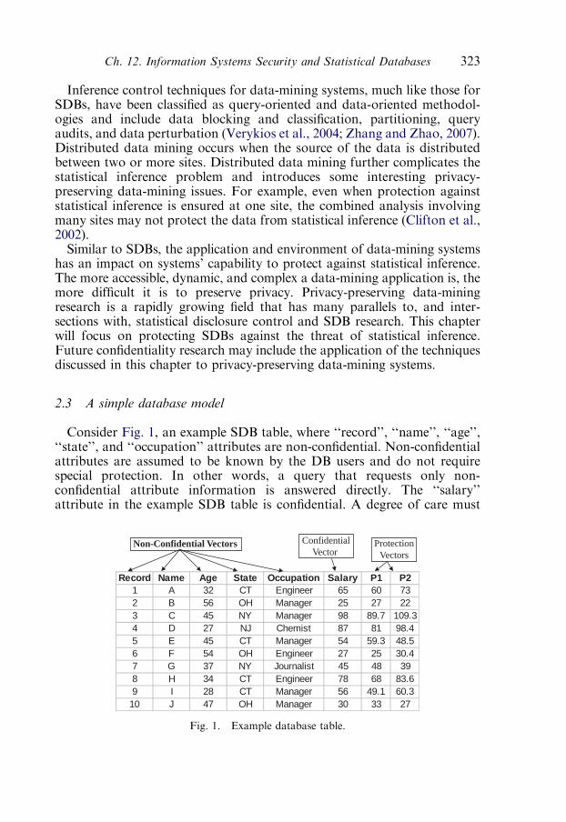
Inference control techniques for data-mining systems, much like those forSDBs, have been classified as query-oriented and data-oriented methodol-ogies and include data blocking and classification, partitioning, queryaudits, and data perturbation (Verykios et al., 2004; Zhang and Zhao, 2007).Distributed data mining occurs when the source of the data is distributedbetween two or more sites. Distributed data mining further complicates thestatistical inference problem and introduces some interesting privacy-preserving data-mining issues. For example, even when protection againststatistical inference is ensured at one site, the combined analysis involvingmany sites may not protect the data from statistical inference (Clifton et al.,2002).Similar to SDBs, the application and environment of data-mining systems
has an impact on systems’ capability to protect against statistical inference.The more accessible, dynamic, and complex a data-mining application is, themore difficult it is to preserve privacy. Privacy-preserving data-miningresearch is a rapidly growing field that has many parallels to, and inter-sections with, statistical disclosure control and SDB research. This chapterwill focus on protecting SDBs against the threat of statistical inference.Future confidentiality research may include the application of the techniquesdiscussed in this chapter to privacy-preserving data-mining systems.
2.3 A simple database model
Consider Fig. 1, an example SDB table, where ‘‘record’’, ‘‘name’’, ‘‘age’’,‘‘state’’, and ‘‘occupation’’ attributes are non-confidential. Non-confidentialattributes are assumed to be known by the DB users and do not requirespecial protection. In other words, a query that requests only non-confidential attribute information is answered directly. The ‘‘salary’’attribute in the example SDB table is confidential. A degree of care must
Record Name Age State Occupation Salary P1 P21 A 32 CT Engineer 65 60 732 B 56 OH Manager 25 27 223 C 45 NY Manager 98 89.7 109.34 D 27 NJ Chemist 87 81 98.45 E 45 CT Manager 54 59.3 48.56 F 54 OH Engineer 27 25 30.47 G 37 NY Journalist 45 48 398 H 34 CT Engineer 78 68 83.69 I 28 CT Manager 56 49.1 60.3
10 J 47 OH Manager 30 33 27
ConfidentialVector
ProtectionVectors
Non-Confidential Vectors
Fig. 1. Example database table.
Ch. 12. Information Systems Security and Statistical Databases 323
be taken when answering queries that use information specific to a confi-dential attribute. For instance, a query, Q1 requesting a count of the recordsof subjects from Connecticut could be answered directly. However, careshould be taken in answering a query, Q2, requesting a count of subjectswith a salary over 50 because this query involves confidential information.Also in Fig. 1 there are two protection attributes, P1 and P
2, explained inSection 4, that exist for the sole purpose of protecting the confidentialattribute. In the example DB there are n ¼ 10 records, five non-confidentialattributes, one confidential attribute, and k ¼ 2 protection attributes.
2.4 Statistical inference in SDBs
There are a variety of logical and statistical methods that an attacker mayuse in attempts to deduce the values of protected sensitive information. Anattacker may try to discover protected data using insider information (that is,prior knowledge of either some of the protected data or some aspect of theprotection algorithm). The attacker may very well be a legitimate user of thesystem who has access to some of the information in the SDB, but isrestricted from direct access to other more sensitive information. Hence,understanding disclosure risk and protecting against it is difficult not onlybecause of the complexity of the problem itself, but also due to the difficultiesin making assumptions about the disclosure threats and information needs ofthe users (Willenborg and de Waal, 2001).Attacks often take on the characteristic of a sequence of apparently
innocuous queries. Each query during the attack might appear to be alegitimate query that in and of itself does not leak any of the protectedinformation. For example, consider the following sequence of queries to theexample SDB above by an attacker with no insider information who desiresexact salary knowledge of person ‘‘F’’. We can assume that all OS andapplication levels of security are effective, however, the user is allowed accessto information aggregated from the sensitive information (COUNT andSUM) because this information is required by the user to execute her officialduties. Note that in this sequence of queries, no single query alone disclosesindividual salary information.
Query 1: Name, state, occupation and salary of every employee.Answer: All data is provided.
Query 2: Average salary of Ohio employees. Answer: 27.3334.Query 3: Number of Ohio employees. Answer: 3.Query 4: Average salary of Ohio managers. Answer: 27.5.Query 5: Number of Ohio managers. Answer: 2.
An attacker could quickly infer from these queries that the salary ofemployee F is 27. This simple illustration shows an SDB’s vulnerability to theindirect disclosure of a sensitive datum by an attacker with no prior
R. Garfinkel et al.324
knowledge of the information (but, as a legitimate user who may have someinsider knowledge of the protection algorithm or at least how queries areanswered). The problem arises because SDBs balance user access with dataprotection. In this example, there is a simple protection algorithm that says‘‘do not answer singleton queries’’. This example illustrates a very simpleattack that prevails over a naive protection mechanism. Of course, there aremore sophisticated measures that can be taken to protect information againstattacks. We discuss some of these measures in the following section.Eventually, the DB administrator (DBA) is forced to make a trade-off of‘‘data loss’’, a degradation of information quality, in exchange for increaseddata protection. The remainder of this chapter will focus on techniquesavailable for the protection of sensitive information in SDBs.
3 Protecting against disclosure in SDBs
Inferential disclosure (henceforth referred to as disclosure) refers to theability of an attacker to infer either the identity of an entity to which aparticular record belongs (re-identification) or the value of a confidentialvariable (predictive disclosure) as described by Willenborg and de Waal(2001). Disclosure can be complete or partial. Complete disclosure, alsocalled exact disclosure, is said to occur if the exact value of a sensitive datumis revealed. Partial disclosure may also be referred to as ‘‘statisticaldisclosure’’. Beck (1980) states that statistical disclosure is said to occur ifinformation from a sequence of queries makes it possible to obtain a betterestimate for a sensitive data point than would have been possible from onlya single query. Delanius (1977) comments that disclosure control in SDBsrefers to a systems ability to provide answers, usually as point estimates, touser’s queries while necessitating a large number of independent samples toobtain a small variance of the estimator.Adam and Wortmann (1989) discuss the adequacy of disclosure control
mechanisms and state that in order for disclosure control to be acceptable itmust prevent exact disclosure while providing statistical disclosure control.If there is a common theme in the various views of disclosure control, it isthat any disclosure control technique must consider both exact disclosureand partial disclosure. Further, while the issue of protecting against exactdisclosure is relatively clear, protecting against partial disclosure is less clearand this implies that there is an acceptable range of statistical protection thatcould vary from no disclosure to some level of disclosure.While the level of partial disclosure is imperative when discussing the
adequacy of a disclosure control mechanism, it is not the only factor toconsider. The next most obvious factor to consider is the level of ‘‘informa-tion loss’’ (Adam and Wortmann, 1989). There are also several otheradditional factors to be considered including the system robustness, ability toprotect data (numerical and categorical), ability to protect more than one
Ch. 12. Information Systems Security and Statistical Databases 325
attribute, suitability for the protection dynamic SDBs, richness of informa-tion given in answers to queries, cost of implementation, and overall usability(Adam and Wortmann, 1989). Ultimately, a DBA may decide that partialdisclosure is acceptable because it may be the only way to balance thedisclosure control with the other performance factors.
3.1 Protecting against statistical inference
Approaches to protecting against statistical inference in SDBs can bedivided into four general categories; conceptual, data masking, queryrestriction, and camouflaging techniques. In implementation, theseapproaches are sometimes combined to increase effectiveness. Conceptualtechniques for data protection are introduced in the conceptual design phaseof the DB. Two common types of conceptual techniques are the latticemodel and conceptual partitioning (Chin and Ozsoyoglu, 1981). Queryrestriction refers to restricting answers to queries that could potentially leadto disclosure of confidential data. Query restriction is discussed in Chin andOzsoyoglu (1982), Dobkin et al. (1979), Fellegi (1972), Gopal et al. (1998),Hoffman and Miller (1970), and Schlorer (1980). Data masking techniquesare introduced and discussed in Beck (1980), Denning (1980), Lefons et al.(1982), Leiss (1982), Liew et al. (1985), Muralidhar et al. (1995), Reiss(1984), and Schlorer (1981). Data masking refers to the changing ofnumerical data systematically so that a user querying the data cannotdetermine confidential data with certainty.Camouflage techniques ‘‘hide’’ the confidential data within a larger data
set and answers queries with respect to that set. Users are then provided withintervals that are guaranteed to contain the exact answer. Thus, thesetechniques are related to query restriction in that query answers are‘‘deterministically correct’’ while eliminating the need to ever refuse toanswer a query. The latter property is shared with data masking techniques,as is the down side that query answers are not generally exact (pointanswers). Gopal et al. (2002) introduce the Confidentiality Via Camouflage(CVC) approach for confidential numerical data.As previously mentioned, each of the above data confidentiality methods
has advantages and disadvantages. Conceptual and query restrictiontechniques offer effective protection and the answers given are correctbecause they are exact answers; however, often these techniques requiresome queries not to be answered. Data masking techniques allow for allqueries to be answered, however, the answers given are not exact and candiffer significantly from the exact answers especially in the case of queries ofsmall cardinality. CVC’s major advantage is that it will give deterministicallycorrect answers to an unlimited number of user queries. However, CVCtechniques are sometimes vulnerable to ‘‘insider information’’ threats. Theseare threats due to prior knowledge some sensitive data or of the CVCtechnique, specifically knowledge of the parameters used in the technique.
R. Garfinkel et al.326
3.2 The query restriction approach
Query restriction techniques protect sensitive data by enforcing rulesrestricting the type and number of queries answered. One very simpletechnique is based on query size, where queries of very small size or verylarge size are not answered. For instance, the earlier example query‘‘Average salary of all the engineers from Ohio’’ would not be answeredbecause the cardinality (the number of records used in the query) is one.Similarly, the query ‘‘Average salary of all employees’’ would not beanswered because a follow-up query such as ‘‘Average salary of allemployees who are not journalists’’ would allow a user to quickly inferthe journalists salary.However, Friedman and Hoffman (1980) point out that simple query
restriction alone may not guarantee confidentiality. They proposed anexpanded query-set size control mechanism that takes into account thelogical relationship between separate queries and determine an ‘‘impliedquery set’’. However, it is easy to show that the number of implied querysets grows exponentially with the number of attributes and thereforecalculating and storing the implied query sets could be exorbitantlyexpensive in terms of computation and storage. Furthermore, it has beenshown that sensitive statistic can still be inferred from allowed query answers(Denning, 1982).Query-set overlap techniques were developed to overcome this problem
(Schlorer, 1976). However, these techniques are burdensome because theyrequire extensive auditing and comparing incoming queries with all thequery answers previously released. Other approaches to this type of queryrestriction include using an audit expert system (Chin and Ozsoyoglu, 1982)and the combination of query restriction and conceptual design techniquesthat take into account the number of attributes such as logical partitioningand cell suppression.
3.3 The data masking approach
The general idea of data masking is to modify the confidential data. Insome realizations the replacement data are also from the same confidentialfield. In that case the technique is called data swapping or data shuffling(Muralidhar and Sarathy, 2006). When the data does not come from theconfidential field, but is randomly generated, the name perturbation is oftenused. There are a number of ways that the sensitive data may be perturbed.For instance, one technique is to view the sensitive numerical data in a SDBas a sample belonging to a distribution of a population. Then by eitherreplacing the ‘‘exact’’ sample with another sample from the samedistribution or by simply using the distribution, rather than the exact data,to answer queries disclosure of ‘‘exact’’ information can be avoided. Data
Ch. 12. Information Systems Security and Statistical Databases 327

masking can allow for unlimited query answers, thus, allowing more queriesto be answered than would query restriction techniques.
3.4 The confidentiality via camouflage (CVC) approach
In CVC, protection of confidential data is termed ‘‘interval protection’’because each confidential datum is guaranteed protection in the form of aninterval (Garfinkel et al., 2002). That is, for the ith given confidential datumai, an interval ½‘i; ui� is established such that ai 2 ½‘i; ui�, and that no user willbe able to determine from the answers to queries that ai4‘i or that aioui.The values ‘i and ui are set by the ith user. Interval answers to queryfunctions are given by minimum and maximum of the functions over aconvex, compact (closed and bounded), set that contains the confidentialvector, thus assuring that answers will be deterministically correct. Detailsare given in the next section.
4 Protecting data with CVC
Suppose a DB user submits a query Q to the DBA. Query selectionresults in the query set T(Q), which is a subset of all records in the DBN ¼ {1, 2, . . . , n}. T(Q) is of cardinality t, and TðQÞ N. The confidentialvector is denoted a. A query Q corresponds to a function over the record setT(Q) which is denoted as f Qð�Þ. If the query Q is over the query set of actualvalues a, its corresponding answer is f QðaÞ.If the data involved in the query is not confidential, the query is answered
exactly. Consider Query A in the following example.
Example 1. Answering a SUM query: A user submits query QS: The sumof the salaries of the engineers to the DBA (who answers queries usingthe example SDB table, Fig. 1). T(QS) ¼ {1, 6, 8}, t ¼ 3, f QS
ðaÞ ¼P
i2TðQSÞ
ai ¼ 170.
Consider protecting the private vector a using the vector set P where
P :¼ convðPÞ ¼ x : x ¼Xkj¼1
ljPj;Xkj¼1
lj ¼ 1; lj � 0
( )
is the convex hull of the vectors in P ¼ P1; . . . ;Pk �
. The protectionvectors are created so that a 2 P to ensure that query answers aredeterministically correct. Also, the protection vectors are chosen to providea level of protection guaranteed to the DB subjects. That is, for each i thereis at least one p j
i � ‘i otherwise a user will be able to infer that ‘iominfp ji :
1 � j � kg ¼ minfxi : x 2 Pg � ai. Similarly, for each i there is at least onep ji � ui otherwise a user will be able to infer that ui4maxfp j
i : 1 � j � kg ¼
R. Garfinkel et al.328

maxfxi : x 2 Pg ¼� ai. Query responses are given as answer intervalsIQ ¼ ½r
L; rU �, where
rL :¼ minf f QðxÞ : x 2 Pg (1)
rU :¼ maxf f QðxÞ : x 2 Pg (2)
To ensure protection it is necessary for a to be a point in the relative interiorof P. This can be accomplished by choosing arbitrary vectors P1; . . . ;Pk�1
and strictly positive numbers g1; . . . ; gk such thatPk
j¼1 gj ¼ 1, and thensetting
Pk :¼ a=gk �Xk�1j¼1
ðgj=gkÞPj
Figure 2 shows the CVC protection vectors for k ¼ 3 where P1 and P2 arefrom Fig. 1 and g1 ¼ 0:3; g2 ¼ 0:5; and g3 ¼ 0:2.
4.1 Computing certain queries in CVC
Gopal et al. (2002) provide methods to determine interval answers forVAR, MIN, MEDIAN, PERCENTILE, and REGRESSION queries.These methods include four classes of algorithms: (1) extreme point evalua-tion (used for SUM queries), (2) very efficient algorithms that are minimalaccess and time bounded by a low order polynomial in k (used for VARqueries), (3) grid search (REGRESSION query), and (4) bounding heuris-tics, fast minimal access heuristics that yield ½r�; rþ� where r� � rL andrþ � rU (used for MIN queries). We briefly introduce these methods by wayof several examples (see Fig. 3 and Examples 2–4 below).
Record P1 P2 P3 a1 60 73 52.5 652 27 22 29.5 253 89.7 109.3 82.2 984 81 98.4 67.5 875 59.3 48.5 59.8 546 25 30.4 21.5 277 48 39 55.5 458 68 83.6 79 789 49.1 60.3 55.6 56
10 33 27 33 30
Fig. 2. Database table with a in the relative interior of P.
Ch. 12. Information Systems Security and Statistical Databases 329

Example 2. QS: The sum of the salaries of the engineers. T(QS) ¼ {1, 6, 8},and t ¼ 3. We have
rU ¼ max1� j�k
Xi2TðQSÞ
pji
8<:
9=; ¼ 73þ 30:4þ 83:6 ¼ 187
rL ¼ min1� j�k
Xi2TðQSÞ
p ji
8<:
9=; ¼ 60þ 25þ 68 ¼ 153
and the answer is given as the interval IQS¼ ½rL; rU � ¼ ½153; 187� (exact
answer is 170).
Example 3. QM: The minimum of the salaries of the engineers. T(QM) ¼{1, 6, 8}, and t ¼ 3. MIN is a concave function and so, rL is achieved atan extreme point of P, that is,
rL ¼ min1�j�k
mini2TðQSÞ
pji
� �¼ 21:5
However, computing rU would require solving a linear program with kþ1variables (4 in this example) and t constraints (3 in this example). Since tmay be large, a bounding heuristic is used
rU ¼ mini2TðQSÞ
max1�j�k
p ji
� �¼ 30:4
and the interval answer is IQM¼ ½rL; rU � ¼ ½21:5; 30:4� (exact answer
is 27).
Example 4. QV: The variance of the salaries of the engineers. T(QV) ¼{1, 6, 8}, and t ¼ 3. In this case VAR is a convex function and so, rU isachieved at an extreme point of P, that is,
rU ¼ max1�j�k
1
t
Xi2TðQÞ
p ji � �p j
2( )¼ 552:2
Record State Occupation a p1 p2 p31 CT Engineer 65 60 73 52.56 OH Engineer 27 25 30.4 21.58 CT Engineer 78 68 83.6 79
351781351071MUS
Fig. 3. Selected DB table used for Examples (2)–(4).
R. Garfinkel et al.330
To compute rL it is necessary to solve a quadratic program, namely,
rL ¼ min1
t
Xi2TðQÞ
Xkj¼1
ljðpji � �p jÞ
!2
:Xkj¼1
lj ¼ 1; lj � 0
8<:
9=; ¼ 348:7
and the interval answer is IQV¼ ½rL; rU � ¼ ½348:7; 552:2� (exact answer is
468.2).
4.2 Star
Star is a variation of CVC. In CVC protection is implemented through acamouflaging set that is a polytope, while Star protection is implementedthrough an n-dimensional union of n line segments intersecting at a commonpoint. The adjective ‘‘star’’ originates from the resemblance of the protectionset to a multi-dimensional star. There are two major advantages of the Startechnique: first, it protects confidential data against insider informationthreats, and second, it is a more flexible technique in that the protectionbounds may be easily manipulated in order to generate smaller answerintervals. Protecting against insider data information is a very desirableproperty. However, Star is vulnerable to insider algorithm information. Inother words, the Star pseudo code must not be known to users.Concretely, Star uses a protection set P defined as
P :¼[i2N
Si
where each Si is the line segment
Si :¼ a� ðai þ aui þ ð1� aÞ‘iÞei : a 2 0; 1� �
and ei is the ith unit n-vector. In words Si is the line segment in which allelements of a except for ai retain their original values, while the ith elementtakes on all values in the range ½‘i; ui�. It follows that for any query Qcorresponding to the function fQ and the set T(Q), the answer interval IQcan be computed by minimizing and maximizing fQ over all Si, i 2 TðQÞ,and then concatenating the t answer intervals.We repeat the following example to illustrate the Star solution for a SUM
query submitted to the example SDB table.
Example 5. QS: The sum of the salaries of the engineers. T(QS) ¼ {1, 6, 8},and t ¼ 3. Three sets are generated, the SUM is calculated providing ananswer interval for each set in Table 1. The interval answer for the query isIQS¼ ½148; 202�.
Ch. 12. Information Systems Security and Statistical Databases 331

Note that for a large-size query, the creation of the line segments andoptimizing over each segment may become unwieldy, even though thecalculations are very straightforward. Therefore, exact algorithms that areO(t) and minimal access have been developed for some common querytypes including SUM, COUNT, and VARIANCE (Garfinkel et al., 2006a).
5 Linking security to a market for private information—A compensationmodel
5.1 A market for private information
The purpose of SDBs and data-mining systems is to extract data(sometimes from various sources), analyze data, and present the informationand knowledge gleaned from analysis to the systems’ users. When the datacollected and analyzed is of a personal nature, this introduces confidentialityproblems in SDBs and the problem of privacy preservation in data mining.Most individuals consider privacy as a guarantee that their personalinformation will not be misused. One way that the administrators of SDBs,and data-mining applications, can ensure that subjects (the individualsproviding their personal data, one way or another, to the system) do nothave their privacy violated is to fairly compensate them for the use of theirinformation. For example, some marketing firms have been compensatingusers for the collection and use of personal data in creating marketinginformation using ‘‘freebies’’ such as free Internet access, e-mail service, andeven computers; all in exchange for individuals’ private information (Changet al., 1999).Laudon (1996) introduces the concept of a National Information
Marketplace (NIM), a marketplace that would have the capability oftracking individuals’ private information and compensating these indivi-duals for use of their private information. Varian (1996) explores marketsfor personal information, like the NIM depicted by Laudon, from aneconomic perspective. These personal information markets, however,require the control of confidentiality as well as fair compensation. Therefore,a compensation mechanism that protects subjects’ privacy while providing
Table 1
CVC-Star computation for SUM example
Record Set 1 Set 2 Set 3
1 50–90 65 65
6 27 5–45 27
8 78 78 70–110
SUM 155–195 148–188 162–202
R. Garfinkel et al.332

compensation to the subjects is necessary for the creation of sustainablepersonal information markets. This section demonstrates a compensationmodel based on the CVC approach.
5.2 Compensating subjects for increased risk of disclosure
We develop subject compensation models that are based on the reductionin protection intervals (Garfinkel et al., 2006a,b). We model the decrease inthe protection interval as a proxy for an increased risk of disclosure. In ourmodels, the compensation details are agreed upon between a third partytrusted information intermediary (TII) and each subject. The details of theagreement, and the resulting compensation model, influence the degreeof control subjects exert over the level of disclosure of their privateinformation. Varying degrees of subject control may be achieved throughmore detailed agreements and the associated implementations. The way thatthe TII manipulates, bounds, and compensates subjects has a great impacton the TII’s production costs. The TII should set a price of compensationsuch that subjects have incentive to participate. We look at twocompensation models that we call ‘‘elastic’’ and ‘‘inelastic’’. Answer qualityis defined to be flexible if the TII allows ‘‘constrained queries’’, where theconstraint is an upper limit on the range of the answer interval. For exampleconsider again the query QS: the sum of the salaries of the engineers. Basedon the data from Table 1 the exact answer is 170, the interval answer fromStar is [148, 202], and the range of the interval is 202�148 ¼ 54. An exampleof a constrained query would occur when a user requests the range of theanswer interval to be less than or equal to 40, that is, a 26% reduction withrespect to the initial answer range.Additionally, consistency in answering queries involving shrinking of
protection bounds is critical. This is, if a user is provided with two differentanswers to the same query then the user could infer additional information.For instance, by intersecting overlapping intervals resulting from incon-sistent answers a user could expose a DB to additional inference threat.Therefore, queries requiring reductions in protection bounds should besystematically answered so that the answers to the same queries areconsistent. The nature of the Star model guarantees consistent answers.Elastic ‘‘Memoryless’’ shrinking and compensation: Elastic bound manipu-
lation is considered to be ‘‘memoryless’’ or resilient in the sense that eachquery is answered individually and any adjustment to protection bounds inanswering the query is forgotten as soon as the query has been answered.After a query is answered the TII compensates the appropriate subjects andthe DB is rolled back to its original protection state. Subsequent queryanswers would be based on the original protection state. Subjects arecompensated each time a query answer compromising their protectionbounds is given.
Ch. 12. Information Systems Security and Statistical Databases 333
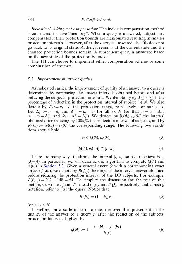
Inelastic shrinking and compensation: The inelastic compensation methodis considered to have ‘‘memory’’. When a query is answered, subjects arecompensated if their protection bounds are manipulated resulting in smallerprotection intervals. However, after the query is answered, the DB does notgo back to its original state. Rather, it remains at the current state and thechanged protection bounds remain. A subsequent query is answered basedon the new state of the protection bounds.The TII can choose to implement either compensation scheme or some
combination of the two.
5.3 Improvement in answer quality
As indicated earlier, the improvement of quality of an answer to a query isdetermined by comparing the answer intervals obtained before and afterreducing the subjects’ protection intervals. We denote by yi, 0 � yi � 1, thepercentage of reduction in the protection interval of subject i 2 N. We alsodenote by Ri :¼ ui � li the protection range, respectively, for subject i.Let D�i :¼ li � ai and Dþi :¼ ui � ai for all i 2 N (so that li ¼ ai þ D�i ,ui ¼ ai þ Dþi , and Ri ¼ Dþi � D�i ). We denote by ½liðyiÞ; uiðyiÞ� the intervalobtained after reducing by 100yi% the protection interval of subject i, and byRiðyiÞ :¼ uiðyiÞ � liðyiÞ the corresponding range. The following two condi-tions should hold
ai 2 liðyiÞ; uiðyiÞ� (3)
½liðyiÞ; uiðyiÞ� � ½li; ui� (4)
There are many ways to shrink the interval ½li; ui� so as to achieve Eqs.(3)–(4). In particular, we will describe one algorithm to compute liðyiÞ anduiðyiÞ in Section 5.3. Given a general query Q with a corresponding exactanswer f QðaÞ, we denote by Rð f QÞ the range of the interval answer obtainedbefore reducing the protection interval of the DB subjects. For example,Rðf QS
Þ ¼ 202� 148 ¼ 54. To simplify the discussion for the rest of thissection, we will use f and T instead of fQ and T(Q), respectively, and, abusingnotation, refer to f as the query. Notice that
RiðyiÞ ¼ ð1� yiÞRi (5)
for all i 2 N.Therefore, on a scale of zero to one, the overall improvement in the
quality of the answer to a query f, after the reduction of the subjects’protection intervals is given by
qðYÞ :¼ 1�f þðYÞ � f �ðYÞ
Rðf Þ(6)
R. Garfinkel et al.334

where Y :¼ ðy1; . . . ; ynÞ,
f�ðYÞ :¼ inf f ðx;TÞ : x 2 SðYÞ �
(7)
f þðYÞ :¼ supff ðx;TÞ : x 2 SðYÞg (8)
and SðYÞ is the Star protection set obtained from using the subject intervals½liðyiÞ; uiðyiÞ�, i 2 N.
5.4 The compensation model
Let M denote an index set to refer to the users and Fm denote an index setfor the queries requested by user m 2M. A user is charged a price pf foreach record accessed to answer a query f 2 FM and a price si proportionalto the reduction of the ith protection interval. The user’s profit functionafter shrinking the protection intervals is given by
Pm :¼Xf2Fm
Bm qðYfÞ; jTf j
� pf jTf j �
Xi2Tf
siyfi
0@
1A (9)
Here Bm is a function of query cardinality and answer quality representingthe user’s utility from the interval answer to a given query, and Y f is thevector of interval shrinkages from query f. We assume that Bm is twice-continuously differentiable, concave, and non-decreasing in both coordinates.The total revenue from the users of the system is
Ptotal :¼Xm2M
Xf2Fm
pf jTf j þXi2Tf
siyfi
0@
1A (10)
Of these total revenues the TII pays the subjects a fraction 1� b, whereb 2 ½0; 1�, that is, generated from the shrinking of the protection intervals.Therefore the remaining proceeds, namely
PTII :¼Xm2M
Xf2Fm
pf jTf j þ bXm2M
Xf2Fm
Xi2Tf
siyfi (11)
constitute the revenues of the TII. The revenue of subject i is
Pi :¼ ð1� bÞsiXm2M
Xf2Fm;Tf3i
y fi (12)
Ch. 12. Information Systems Security and Statistical Databases 335
If the quality improvement function qðYÞ is differentiable, then we obtainfirst-order optimality conditions for the mth user’s profit, namely,
@Bm
@qqðY fÞ; jTf j
@q@y f
i
ðY fÞ � si ¼ 0 (13)
for all f 2 Fm and i 2 Tf .Eq. (13) indicates that user m’s quality choice will depend on the change in
the user’s benefit with respect to quality, the change in protection intervals,and the cost of protection reduction. By re-arranging terms, we get
@q
@y fi
ðY fÞ ¼
si
@Bm qðY fÞ; jTf j
=@q
(14)
which indicates that, for a given query f, the optimal reduction in theprotection interval for subject i is found when the change in overall qualityof the answer to the query matches the ratio of the unit reduction cost of thesubject’s interval to the marginal utility of user m. Roughly speaking, whenthe subject’s unit reduction cost exceeds the user’s marginal utility, thenequilibrium is achieved at a point where the query answer quality curve, as afunction of interval reduction is steep. In other words equilibrium is found ata point where there are considerable gains in quality achieved by smallreductions in interval size. On the other hand, when the unit reduction cost isbelow the utility margin, equilibrium is achieved at a point where the qualitycurve is close to flat, that is, when there is little to gain from small reductionsin interval size.Note that subject i receives revenue only if the data point ai is used in the
calculations of query answers. The determination of whether that happens isindependent of the unit price si and the protection interval ½li; ui�, unless theuser requests shrinking of the answer interval. In that case if either si is toohigh or ½li; ui� is too wide, the total price of shrinking may be so high that theuser will refuse to pay, and thus no compensation will accrue to subject i.Therefore the subjects are motivated to be honest in terms of both theirrequired costs and levels of protection. We formalize that concept with thefollowing proposition, the proof of which can be found in (Garfinkel et al.,2006b). As a consequence of this result, it is clear that there is no incentive fora DB subject to arbitrarily increase her protection interval. Also there is noincentive for either the TII or the subjects to arbitrarily increase the prices si.
Proposition 6. Given an arbitrary query, a fixed user desired answer qualitylevel for the query, and a fixed subject i for whom the protection interval hasbeen reduced, then
� there exists a constant si such that PTII and Pi are linear, strictlyincreasing functions of si, for si � si, and PTII ¼ Pi ¼ 0, for si4si;
R. Garfinkel et al.336

� there exists a constant ri such that PTII and Pi are increasingfunctions of Ri, for Ri � ri, and PTII ¼ Pi ¼ 0, for Ri4ri
5.5 Shrinking algorithm
The Star method has the advantage that it can quickly calculate answers ofvarying quality levels to satisfy user demand. The following generic algorithmprovides optimal, i.e., minimum cost, reductions of subject protectionintervals to achieve a desired level of quality of the answer to a given query.
Star shrinking algorithm:
Input parameters : q; 1; u;T ; and a query f :
Output parameters : ð f �ðYÞ; fþðYÞÞ
Algorithm body :
Y ~0;
for each i 2 T doRi ui � li;
stop false;
while not stop do;
stop true;
M� fi 2 T : f�i ðYÞ ¼ f �ðYÞg;
Mþ fi 2 T : fþi ðYÞ ¼ f þðYÞg;
find increment y in lower bound I;
for each i 2M�do
li li þ yRi;
Yi þYi þ y;
end for;
if qðYÞ � q then return ð f �ðYÞ; f þðYÞÞ;
find decrement y in upper bound u
for each i 2Mþdo
ui ui þ yRi;
Yi Yi þ y;
end for;
if qðYÞ � q then return ðf�ðYÞ; f þðYÞÞ;
if y40 then stop false;
end while
Ch. 12. Information Systems Security and Statistical Databases 337

In the algorithm, q represents a user’s desired quality improvement levelfor a given query f . The algorithm will return a pair ðf �ðYÞ; f þðYÞÞcorresponding to a Star interval answer with improvement of at least q. Ateach iteration the algorithm first tries to increase a collection of protectionlower bounds to reduce the overall size of the protection set and thus toimprove the quality of the Star answer to the query. If the increment in thelower bounds is not enough, then the algorithm tries to decrease a collectionof protection upper bounds to additionally reduce the size of the originalprotection set. The algorithm iterates until the original protection set issufficiently reduced in size as to achieve the desired quality level q. Since thealgorithm can potentially reduce the original protection set to just one point(the confidential vector a), its finiteness is guaranteed.To find the increment in the chosen lower bounds at each iteration, the
variable y is increased as long as three conditions are satisfied: theconfidential values ai remain inside the reduced protection intervals;the lower bounds indexed by M� remain tight; and the overall quality ofthe query improves. A similar procedure is used to determine the amount todecrease the chosen upper bounds at each iteration.Our algorithm is not specific enough to make a precise statement
concerning its complexity. The complexity will depend on how difficult it isto find the increment and decrement amounts in the lower and upperbounds, respectively, at each iteration. It also depends on the complexity ofcomputing the Star answer interval for a given query f and correspondingquery set T. For common queries such as: SUM; MEAN; STANDARDDEVIATION; MIN (MAX); REGRESSION, the Star structure allowscomputations at each iteration to be extremely fast. For example, for SUMqueries, the Star answer requires OðjT jÞ computations at each iteration.Then the y required to increase the corresponding lower bounds can befound by computing
g�ðYÞ :¼ min f �i ðYÞ : ieM� �
(15)
y :¼ min max g�ðYÞ � f�ðYÞð Þ=Ri;�D�i =Ri
�: i 2M�
�(16)
Likewise, a similar formula can be established to determine the y requiredto decrease the corresponding upper bounds. Let
R :¼ max Ri : i 2 T �
� :¼ min jD�i � D�j j : D�i aD�j ; jD
þi � Dþj j : D
þi aDþj
n othen the algorithm applied to a SUM query will take OðR=�Þ iterations inthe worst case. It follows that the shrinking algorithm applied to a SUMquery would take OðRjT j=�Þ computations.
R. Garfinkel et al.338

In general, for random or unstructured interval the number of iterationsshould be very small. A very highly structured, worst case scenario wouldbe the following. For a given constant a, suppose that all the subjectintervals are of the form ½a� di; aþ di�, where d14 � � � 4dn, that is, eachinterval is centered at a and interval i strictly contains interval iþ1. Then, atthe end of the kth iteration of the algorithm the quality of the Star answerfor SUM queries will be
qk :¼ 1� dkþ1=d1
Hence, to obtain a desired quality level of q, the algorithm will take kiterations, where k is the first index k for which qk � q, that is,
1� q � dkþ1=d1
When dk decreases ‘‘very slowly’’ the algorithm can take comparatively manyiterations. For example, suppose a user requests q ¼ 0:5 (a 50% reductionwith respect to the original Star answer). If dk ¼ k�0:1, then k ¼ 210 � 1 ¼1023 iterations. Yet, since each iteration will take no more than a fraction ofa second, the answer would still come back very quickly. On the other hand,in practice it is very unlikely to have intervals that exhibit such a ‘‘slow’’decreasing behavior and the algorithm will find an answer in just a fewiterations. For instance, if dk ¼ 10�k, then k ¼ dlnð2Þ=lnð10Þe ¼ 1 iteration.
5.6 The advantages of the star mechanism
Since all aspects of the proposed market have now been illustrated, it isworthwhile to enumerate the beneficial properties of the Star mechanismfor each of the market’s desiderata. In particular these are as follows.Consistency. By its nature, namely minimizing and maximizing the query
function over the set S, the Star mechanism guarantees consistent answers.That is, a user will never be able to achieve additional information by askingthe same query twice and getting different answers.Computational ease. Because of the simple structure of the compact Star
set, exact algorithms for query answers can be developed that are veryefficient. That is, they consist of nothing more than a set of single variablefunction optimizations, and typically can be done in linear time on the sizeof the DB.Safety. It is easy to see that the structure of the Star set also guarantees
that even if a user gains some information about one subject through theshrinking process, that information will be of no use in shrinking theprotection interval of any other subject without compensating that subject.Usefulness for shrinking answer intervals. Star is uniquely designed to
make it simple to determine optimal shrinking in that the effect of shrinkingone subject’s protection interval on the answer interval is immediately seen,and has no effect on the other subjects.
Ch. 12. Information Systems Security and Statistical Databases 339

6 Simulation model and computational results
A simulation model is used to illustrate the compensation model withelastic shrinking. The interaction between flexible quality, privacy protec-tion, and compensation is studied via user demand for SUM queries on thesubjects’ private information. SUM queries are chosen for analysis sincethey represent the most common query type studied in data security models.A typical sequence of events in the simulation starts with a user submitting aSUM query to a DB and a desired quality level for the query answer. TheTII answers the query by adjusting protection bounds where necessary tomeet the requested quality, and calculates the cost of the query and subjectcompensation. Finally, the user decides whether or not to purchase thequery, based on how the user values the query answer and the price chargedby the TII. If the query is purchased, the TII compensates the subjectsaccording to the corresponding percentage b.
6.1 Sample database
We generated a 1000 subject DB containing a private information vector a.The entries of the confidential vector are randomly generated according toa uniform distribution ranging from 10 to 100. We chose the uniformdistribution for the following reasons. Since these models are not statisticalin nature, it seems clear that the distribution of the actual data is not ofparamount importance. That is, the models should allow the market tofunction efficiently independent of the data structure. What we did want toprovide was data that had little structure but a fair amount of variance, forwhich the uniform distribution is ideal. We also note that the uniformdistribution is used to test the models in both Gopal et al. (1998) and Gopalet al. (2002). To further ascertain the robustness of the simulation findings,we replicated our study using a log-normal distribution, another commonlyencountered distribution found in a variety of data. The findings are virtuallyidentical, providing another dimension to support the validity of the findings.Lower and upper protection bounds for the ith subject are also randomly
generated as follows
li :¼ ai 1�Ui=2
ui :¼ li þ ai=2
where Ui has a uniform distribution in ½0; 1�. Note that as ½ai 2 li; ui� andðui � liÞ=ai ¼ 0:5, the generated interval provides a 50% protection level forthe subjects’ confidential data. We assume that the interval reduction priceper subject si is the same for all subjects, that is, si ¼ s for all i 2 N and somepositive value s.
R. Garfinkel et al.340
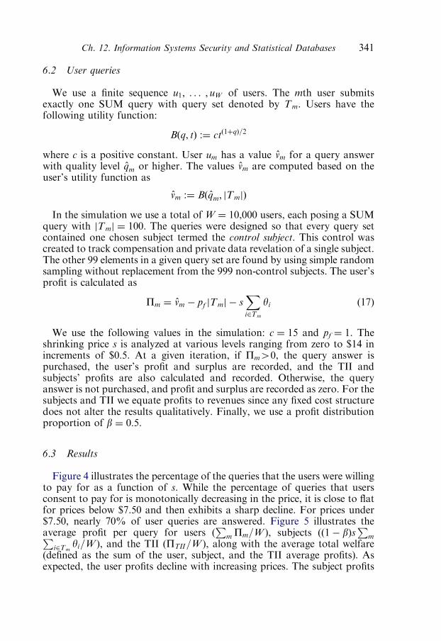
6.2 User queries
We use a finite sequence u1; . . . ; uW of users. The mth user submitsexactly one SUM query with query set denoted by Tm. Users have thefollowing utility function:
Bðq; tÞ :¼ ctð1þqÞ=2
where c is a positive constant. User um has a value vm for a query answerwith quality level qm or higher. The values vm are computed based on theuser’s utility function as
vm :¼ Bðqm; jTmjÞ
In the simulation we use a total of W ¼ 10,000 users, each posing a SUMquery with jTmj ¼ 100: The queries were designed so that every query setcontained one chosen subject termed the control subject. This control wascreated to track compensation and private data revelation of a single subject.The other 99 elements in a given query set are found by using simple randomsampling without replacement from the 999 non-control subjects. The user’sprofit is calculated as
Pm ¼ vm � pf jTmj � sXi2Tm
yi (17)
We use the following values in the simulation: c ¼ 15 and pf ¼ 1. Theshrinking price s is analyzed at various levels ranging from zero to $14 inincrements of $0:5. At a given iteration, if Pm40, the query answer ispurchased, the user’s profit and surplus are recorded, and the TII andsubjects’ profits are also calculated and recorded. Otherwise, the queryanswer is not purchased, and profit and surplus are recorded as zero. For thesubjects and TII we equate profits to revenues since any fixed cost structuredoes not alter the results qualitatively. Finally, we use a profit distributionproportion of b ¼ 0:5.
6.3 Results
Figure 4 illustrates the percentage of the queries that the users were willingto pay for as a function of s. While the percentage of queries that usersconsent to pay for is monotonically decreasing in the price, it is close to flatfor prices below $7.50 and then exhibits a sharp decline. For prices under$7.50, nearly 70% of user queries are answered. Figure 5 illustrates theaverage profit per query for users (
PmPm=W), subjects (ð1� bÞs
PmP
i2Tmyi=W), and the TII (PTII=W), along with the average total welfare
(defined as the sum of the user, subject, and the TII average profits). Asexpected, the user profits decline with increasing prices. The subject profits
Ch. 12. Information Systems Security and Statistical Databases 341
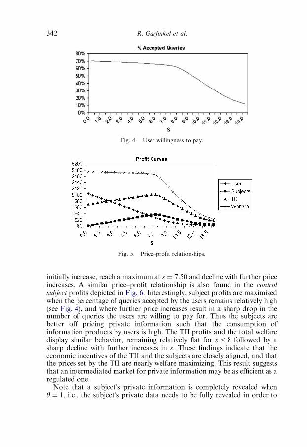
initially increase, reach a maximum at s ¼ 7.50 and decline with further priceincreases. A similar price–profit relationship is also found in the controlsubject profits depicted in Fig. 6. Interestingly, subject profits are maximizedwhen the percentage of queries accepted by the users remains relatively high(see Fig. 4), and where further price increases result in a sharp drop in thenumber of queries the users are willing to pay for. Thus the subjects arebetter off pricing private information such that the consumption ofinformation products by users is high. The TII profits and the total welfaredisplay similar behavior, remaining relatively flat for s � 8 followed by asharp decline with further increases in s. These findings indicate that theeconomic incentives of the TII and the subjects are closely aligned, and thatthe prices set by the TII are nearly welfare maximizing. This result suggeststhat an intermediated market for private information may be as efficient as aregulated one.Note that a subject’s private information is completely revealed when
y ¼ 1, i.e., the subject’s private data needs to be fully revealed in order to
Fig. 4. User willingness to pay.
Fig. 5. Price–profit relationships.
R. Garfinkel et al.342
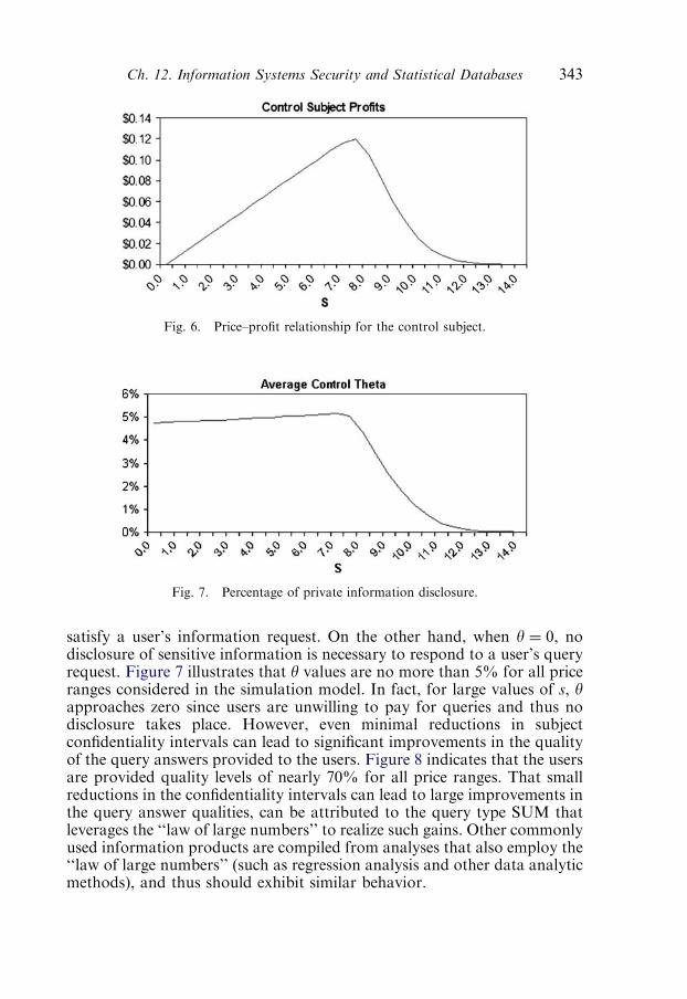
satisfy a user’s information request. On the other hand, when y ¼ 0, nodisclosure of sensitive information is necessary to respond to a user’s queryrequest. Figure 7 illustrates that y values are no more than 5% for all priceranges considered in the simulation model. In fact, for large values of s, yapproaches zero since users are unwilling to pay for queries and thus nodisclosure takes place. However, even minimal reductions in subjectconfidentiality intervals can lead to significant improvements in the qualityof the query answers provided to the users. Figure 8 indicates that the usersare provided quality levels of nearly 70% for all price ranges. That smallreductions in the confidentiality intervals can lead to large improvements inthe query answer qualities, can be attributed to the query type SUM thatleverages the ‘‘law of large numbers’’ to realize such gains. Other commonlyused information products are compiled from analyses that also employ the‘‘law of large numbers’’ (such as regression analysis and other data analyticmethods), and thus should exhibit similar behavior.
Fig. 6. Price–profit relationship for the control subject.
Fig. 7. Percentage of private information disclosure.
Ch. 12. Information Systems Security and Statistical Databases 343

Clearly, the willingness of the subjects to participate (i.e., permit TII toreduce protection intervals) is critical for the market. The incentive for thesubjects to participate comes from the compensation received from the TII.Table 2 illustrates the price impact of the subjects’ reservation values. Forinstance, if the subjects are willing to participate only if they receive, onaverage, $0:02 or more per query to the DB, then it is clear that the TIIneeds to restrict the feasible values for s to lie in the interval ½$3:88; $10:22�.If s is not contained in this interval, the subjects will choose not toparticipate and hence the TII profits resulting from higher quality answersare zero. Interestingly, increasing reservation values on the part of thesubjects drive the prices towards welfare maximizing levels. In summary,the simulation analysis provides an initial validation of the viability ofmarkets for private information.
7 Conclusion
This chapter has outlined some of the major themes in SDB protectionand has focused on protection against the threat of statistical inference.
Fig. 8. Price impact on query quality.
Table 2
Impact of reservation value on feasible prices T
Subject reservation value Range for s
Lower bound ($) Upper bound ($)
0.01 1.94 12.05
0.02 3.88 10.22
0.03 5.84 8.84
R. Garfinkel et al.344

Several protection mechanisms were discussed, with a focus on the CVCprotection model while demonstrating how CVC provides a functional androbust technique to protect online and dynamic SDBs from the inferencethreat. Additionally, the chapter demonstrates how CVC can be linked toan economic model for the intermediation electronic market for privateinformation.
References
Adam, N.R., J.C. Wortmann (1989). Security-control methods for statistical databases: A comparative
study. ACM Computing Surveys 21(4), 515–586.
Agrawal, R., R. Srikant, (2000). Privacy-preserving data mining, in: Proceedings of the 2000 ACM
SIGMOD Conference on the Management of Data, Dallas, TX, May 14–19, ACM, pp. 439–450.
Beck, L.L. (1980). A security mechanism for statistical databases. ACM Transactions on Database
Systems 5, 316–338.
Castana, S., G.F. Fugini, G. Martella, P. Samarati (1995). Database Security. ACM Press published by
Addison Wesley Longman Limited, England.
Chang, A., P.K. Kannan, A. Whinston (1999). The economics of freebies in exchange for consumer
information on the Internet: An exploratory study. International Journal of Electronic Commerce 4,
p. 1.
Chin, F., G. Ozsoyoglu (1982). Auditing and inference control in statistical databases. IEEE
Transactions on Software Engineering SE-8, 574–582.
Chin, F., G. Ozsoyoglu (1981). Statistical database design. ACM Transactions on Database Systems 6(1),
113–139.
Clifton, C., M. Kantarcioglu, J. Vaidya, X. Lin, M. Zhu (2002). Tools for privacy preserving distributed
data mining. SIGKDD Explorations 4(2), 1–7.
Date, C.J. (2000). An Introduction to Database Systems. 7th ed. Addison Wesley, Reading, MA.
Delanius, T. (1977). Towards a methodology for statistical disclosure control. Statistik Tidskrift 15,
429–444.
Denning, D.E. (1980). Secure statistical databases with random sample queries. ACM Transactions on
Database Systems 5(3), 291–315.
Denning, D.E. (1982). Cryptography and Data Security. Addison Wesley, Reading, MA.
Dobkin, D., A.K. Jones, R.J. Lipton (1979). Secure databases: Protection against user influence. ACM
Transactions on Database Systems 4, 97–100.
Fellegi, I.P. (1972). On the question of statistical confidentiality. Journal of the American Statistical
Association 67, 7–18.
Friedman, A.D., L.J. Hoffman (1980). Towards a failsafe approach to secure databases, in: Proceedings
of IEEE Symposium on Security and Privacy, Oakland, CA.
Garfinkel, R., R. Gopal, P. Goes (2002). Privacy protection of binary confidential data against
deterministic, stochastic, and insider threat. Management Science 48, 749–764.
Garfinkel, R., R. Gopal, D. Rice (2006a). New approaches to disclosure limitation while answering
queries to a database: Protecting numerical confidential data against insider threat based on data or
algorithms, in: Proceedings of 39th Hawaii International Conference on System Sciences (HICSS),
Kuaui, HI.
Garfinkel, R., R. Gopal, D. Rice, M. Nunez (2006b). Secure electronic markets for private information.
IEEE Transactions on Systems Man and Cybernetics, Part A—Special Issue on Secure Knowledge
Management 36(3), 461–472.
Gopal, R., P. Goes, R. Garfinkel (1998). Interval protection of confidential information in a database.
Informs Journal on Computing 10, 309–322.
Gopal, R., P. Goes, R. Garfinkel (2002). Confidentiality via camouflage: The CVC approach to
database security. Operations Research 50, p. 3.
Ch. 12. Information Systems Security and Statistical Databases 345

Hoffman, L.J., W.F. Miller (1970). Getting a personal dossier from a statistical data bank. Datamation
16, 74–75.
Laudon, K. (1996). Markets and privacy. Communications of the ACM 39(9), 92–104.
Lefons, D., A. Silvestri, F. Tangorra (1982). An analytic approach to statistical databases, in:
Proceedings of 9th Conference on Very Large Databases, Florence, Italy, pp. 189–196.
Leiss, E. (1982). Randomizing: A practical method for protecting statistical databases against
compromise, in: Proceedings of 8th Conference on Very Large Databases, Mexico City, Mexico,
pp. 189–196.
Liew, C.K., W.J. Choi, C.J. Liew (1985). A data distortion by probability distribution. ACM
Transactions on Database Systems 10, 395–411.
Muralidhar, K., D. Batra, P.J. Kirs (1995). Accessibility, security, and accuracy in statistical databases:
The case for the multiplicative fixed data perturbation approach. Management Science 41,
1549–1564.
Muralidhar, K., R. Sarathy (2006). Data shuffling—A new masking approach for numerical data.
Management Science 52(5), 658–670.
Palley, M.A., J.S. Siminoff (1987). The use of regression methodology for the compromise of
confidential information in statistical databases. ACM Transactions on Database Systems 12(4),
593–608.
Reiss, S.P. (1984). Practical data swapping: The first steps. ACM Transactions on Database Systems 9,
20–37.
Schlorer, J. (1976). Confidentiality of statistical records: A threat monitoring scheme of on-line dialogue.
Methods of Information in Medicine 15(1), 36–42.
Schlorer, J. (1980). Disclosure from statistical databases: Quantitative aspects of trackers. ACM
Transactions on Database Systems 5, 467–492.
Schlorer, J. (1981). Security of statistical databases: Multidimensional transformation. ACM
Transactions on Database Systems 6, 95–112.
Turn, R., N.Z. Shapiro (1978). Privacy and security in databank systems: Measure of effectiveness,
costs, and protector–intruder interactions, in: C.T. Dinardo (ed.), Computers and Security. AFIPS
Press, Arlington, VA, pp. 49–57.
Varian, H.R. (1996). Economic aspects of personal privacy, from privacy and self-regulation in the
Information Age, Department of Commerce. Available at http://www.ntia.doc.gov/reports/privacy/
selfreg1.htm#1C. Accessed on May 7, 2007.
Verykios, V.S., E. Bertino, I. Fovino, L.P. Provenza, Y. Saygin, Y. Theodoridis (2004). State-of-the-art
in privacy preserving data mining. SIGMOD Record 33(1).
Willenborg, L., T. de Waal (2001). Elements of Statistical Disclosure Control, Lecture Notes in Statistics.
Springer-Verlag, New York.
Zhang, N., W. Zhao (2007). Privacy-preserving data mining systems, Computer, April.
R. Garfinkel et al.346
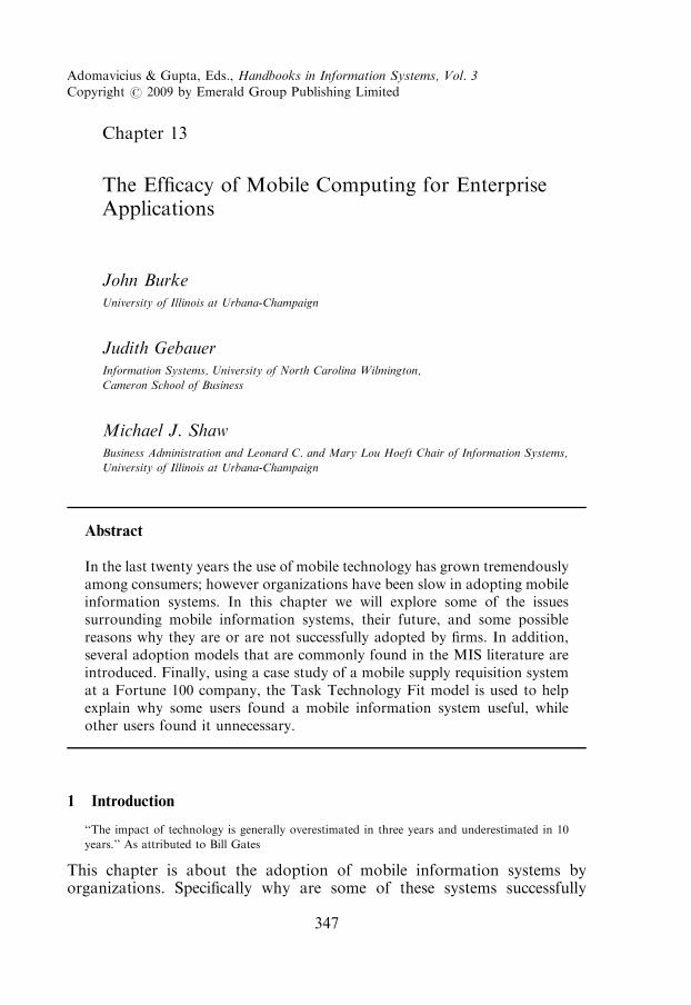
Adomavicius & Gupta, Eds., Handbooks in Information Systems, Vol. 3
Copyright r 2009 by Emerald Group Publishing Limited
Chapter 13
The Efficacy of Mobile Computing for EnterpriseApplications
John BurkeUniversity of Illinois at Urbana-Champaign
Judith GebauerInformation Systems, University of North Carolina Wilmington,
Cameron School of Business
Michael J. ShawBusiness Administration and Leonard C. and Mary Lou Hoeft Chair of Information Systems,
University of Illinois at Urbana-Champaign
Abstract
In the last twenty years the use of mobile technology has grown tremendouslyamong consumers; however organizations have been slow in adopting mobileinformation systems. In this chapter we will explore some of the issuessurrounding mobile information systems, their future, and some possiblereasons why they are or are not successfully adopted by firms. In addition,several adoption models that are commonly found in the MIS literature areintroduced. Finally, using a case study of a mobile supply requisition systemat a Fortune 100 company, the Task Technology Fit model is used to helpexplain why some users found a mobile information system useful, whileother users found it unnecessary.
1 Introduction
‘‘The impact of technology is generally overestimated in three years and underestimated in 10
years.’’ As attributed to Bill Gates
This chapter is about the adoption of mobile information systems byorganizations. Specifically why are some of these systems successfully
347
adopted, while others are not? Another important question for researchersis, what is the future of mobile information systems in organizations?However, before these questions can be addressed it is important to definewhat a mobile information system is. For our purposes, a mobileinformation system is not just the use of mobile devices such as cell phonesby employees of a firm. It is an integrated information system where users,usually a firm’s employees, suppliers or customers, use mobile devices tointeract with the organization, in order to perform some importantfunction(s).
mobile information system: an integrated information system where users, usually a firm’s
employees, suppliers or customers use mobile devices to interact with the organization, in order
to perform some important function(s).
In the last twenty years the growth of mobile technologies has beenphenomenal especially in the consumer market. In part, significantadvances in technology have driven this growth. For example, the first‘‘portable computers’’ were the size of large briefcases; today manypersonal digital assistants (PDA’s) and cell phones can easily fit into apocket. Furthermore, the power and flexibility of these same devices hasincreased dramatically over the same period. Many are even designed toaccess the Internet natively, which did not even exist twenty years ago.Today consumers and organizations have a bewildering array of mobiletechnologies to choose from and the future looks promising. In fact thesedevices are now so popular with the general public that many individuals nolonger have landline phones or desktop computers, preferring to use theirmobile counterparts instead.However, despite success with consumers at home and tremendous
investments in mobile technology by firms, the impact of mobileapplications in organizations has been relatively limited. In this sense,mobile technologies have followed a similar pattern to other revolutionarytechnologies like the railroad, the automobile, the airplane, and theInternet. That is, there have been enthusiastic investments in the beginningwith accompanying high stock prices, followed by disillusionment as firmsdiscovered that their markets and profits took longer than expectedto develop. The Internet bubble is just the latest example of this patternas firms required time to figure out the proper uses and expectations ofE-technologies and lost billions of dollars in the process.In this chapter we will cover several aspects of the use of mobile
technology in organizations. First, some of the current trends in mobiletechnologies are given, along with some predictions for the future. Second,several research frameworks used for evaluating technologies are presented.Third, one study of a mobile application in a Fortune 500 company thathighlights many of the issues facing mobile applications are reviewed.Finally, areas for new research opportunities are discussed.
John Burke et al.348

2 Trends
2.1 Initial experiments in mobile information systems
Early experiments in mobile information systems often failed to live up toexpectations. They tended to be small pilot programs that lacked sufficientscope to yield significant results. Many of the early problems experienced inthese systems stemmed from a lack of IT investment by companies that cutbudgets in response to the recession in 2001.1 However, even with thebudget cuts in many IT departments, mobile information systems havesteadily grown in use as the variety and power of devices available haveincreased. For example, wireless LANs (local area networks) in many urbanareas have become commonplace, car companies sell mobile services suchas OnStar and other global information systems, radio frequencyidentification’s (RFID) are now being used to track assets in factories andwarehouses, and in Europe some ski resorts are even using smart personalobjects embedded in Swatches as electronic ski lift passes.2 Yet even withthis growth many issues still need to be worked out.One issue is that IS/IT managers are sometimes unsure which mobile
technologies are best to adopt given the large number of choices they have inthe marketplace, for example should they choose smart phones or PDAs,Windows- or Linux-based systems, standardize on one type of device orallow employees to choose from a variety of devices, etc. This has led somefirms to adopt a variety of small mobile devices and applications in pilotprograms without giving much thought as to how they would eventually fitinto the overall organization. Such a patchwork of applications is oftendifficult to support or integrate into day-to-day operations. Therefore, it isbeneficial to consider the recent trends in mobile technology before makingnew investments so that a more cohesive mobile strategy can be implemented.
2.2 The trend towards user mobility
Today workers are more dispersed and more on the move more than everbefore. In order to support these employees firms have to deploy technologyto support them. As mentioned above the number and type of mobiledevices has increased dramatically over the last decade. But exactly whatkind of devices a firm should invest in depends a great deal on what kind of
1A survey released in 2001 by Forrester Research showed that the number of large companies inNorth America that had cut their E-Business budgets had nearly doubled. Specifically, Forrester foundin May 2001 that 17% of large companies had decreased their E-Business budgets. Nearly one-third ofGlobal 3500 firms had also reported such reductions. The average reduction was only 0.3% in spring2000, whereas in fall 2001, big companies said that they expected a 6% budget drop.
2Kueppers, A., A. Latour (2000). Watch out phone makers, people are wearing wrist technology. WSJInteractive Edition, April 17.
Ch. 13. Efficacy of Mobile Computing for Enterprise Applications 349

work its employees need to do. Several different types of users and theirusage behaviors have been discussed in the literature, namely wanderers,travelers, and visitors (Sarker and Wells, 2003).Wandering is when users are centered in a place such as an office, but
throughout the day they are away from their desks for substantial amountsof time. For these users the devices need to be small and are used mostly forstaying in touch by phone and perhaps email, i.e. smart phones. Travelersare those who are constantly moving from one place to another likesalespeople. These users require the ability to stay in touch like wanderers,but also need the ability to run more powerful applications like wordprocessors and spreadsheets. Devices such as laptops are common amongtravelers. Finally, visitors are those who do move from one place to another,but not every day, such as executives. Although these users do requiremobility they expect greater functionality from their devices such as full-sizekeyboards and large screens. For these users desktop replacements are moreappropriate. For all of these groups it can be seen that there is a tradeoffbetween functionality and mobility (Gebauer and Shaw, 2002) (Fig. 1).
2.3 The trend towards pervasive computing
Another trend that is entering the workplace is the concept of pervasivecomputing. Pervasive computing is the concept that the ‘‘computer hasthe capability to obtain the information from the environment in which
Fig. 1. Functionality vs. mobility tradeoff.
John Burke et al.350
it is embedded and utilize it to build models of computing’’, and thatthe environment ‘‘can and should also become ‘intelligent’ ’’ and beable to ‘‘detect other computing devices entering it’’ (Lyytinen and Yoo,2002a).Such ‘‘intelligent’’ environments are becoming quite common in the
workplace in the form of RFID tags. RFID tags are used in the same basicway that bar codes are used, to identify objects such as supplies andequipment in an organization. The difference is that bar codes must be readby passing a scanner over them while RFID tags emit their informationelectronically to the scanner when prompted. This allows information to beread much quicker and more accurately than in the past.These tags are being used by companies in various ways. For example,
warehouses use them in pallets and crates to correctly route merchandiseand to determine the weight of trucks, as they are loaded. Walmart inparticular is pushing suppliers in the retail industry to adopt RFID tags toimprove the speed and efficiency of their supply chains. As the power andadaptability of scanners and RFID tags increases more and morecompanies can be expected to be adopt this technology (Angeles, 2005).
2.4 The future: ubiquitous computing
As companies progress in using mobile technology effectively, they willbegin to achieve ubiquitous computing. Ubiquitous computing (Lyytinenand Yoo, 2002b) refers to the combination of the above two trends; namelya large amount of mobility in computer applications combined with a largeamount of environment aware ‘‘intelligent’’ embedded devices. Lyytinenand Yoo suggest that to achieve this will require:
� Large-scale infrastructures.� Computer technologies that share diverse types of data seamlessly withmany different kinds of mobile devices.� Devices that can manipulate diverse types of data effectively even withlimited user interfaces such as small screens and keyboards.� Computer aware environments that provide appropriate services tovarious devices as needed.� Continued improvements in the computing power available in mobiledevices.� Significant increases in the number, quality, and geographic scope ofwireless LANs.� The standardization of the computer protocols used to communicatebetween heterogeneous computer technologies (Fig. 2).
While the rate at which companies adopt mobile technologies may be inquestion it is clear that the trends towards mobile, pervasive, and
Ch. 13. Efficacy of Mobile Computing for Enterprise Applications 351
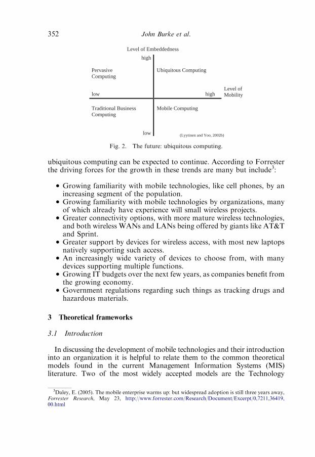
ubiquitous computing can be expected to continue. According to Forresterthe driving forces for the growth in these trends are many but include3:
� Growing familiarity with mobile technologies, like cell phones, by anincreasing segment of the population.� Growing familiarity with mobile technologies by organizations, manyof which already have experience will small wireless projects.� Greater connectivity options, with more mature wireless technologies,and both wireless WANs and LANs being offered by giants like AT&Tand Sprint.� Greater support by devices for wireless access, with most new laptopsnatively supporting such access.� An increasingly wide variety of devices to choose from, with manydevices supporting multiple functions.� Growing IT budgets over the next few years, as companies benefit fromthe growing economy.� Government regulations regarding such things as tracking drugs andhazardous materials.
3 Theoretical frameworks
3.1 Introduction
In discussing the development of mobile technologies and their introductioninto an organization it is helpful to relate them to the common theoreticalmodels found in the current Management Information Systems (MIS)literature. Two of the most widely accepted models are the Technology
Level of Embeddedness
high
PervasiveComputing
low
Ubiquitous Computing
high
Traditional Business Computing
low
Mobile Computing
Level ofMobility
(Lyytinen and Yoo, 2002b)
Fig. 2. The future: ubiquitous computing.
3Daley, E. (2005). The mobile enterprise warms up: but widespread adoption is still three years away,Forrester Research, May 23, http://www.forrester.com/Research/Document/Excerpt/0,7211,36419,00.html
John Burke et al.352

Acceptance Model (TAM) and the Task Technology Fit Model (TTF) model,which are used to predict IT utilization and/or individual performance.
3.2 The technology acceptance model
The idea of the TAM model is that if individuals perceive that atechnology is easy to use and also perceive it as being useful, they will have apositive attitude towards it. This in turn will increase the individual’sintention to use that technology when given the opportunity and finally thiswill lead to actual utilization. The TAMmodel is shown below (Davis, 1989).As can be seen the model also predicts that technology which is perceived asbeing easier to use is also generally seen as being more useful (Fig. 3).
3.3 Example of the technology acceptance model
As an example of how the TAM model works, consider a hypotheticalnon-technical manager given the opportunity to use a basic cell phone, alaptop, or a PDA while traveling. A cell phone today would probably beconsidered easy to use by the average manager and also fairly useful as itwould allow him or her to stay in communication with the office whiletraveling or going to meetings, conferences, etc. Part of the perception ofthe cell phone’s usefulness would be based on the perception that a cellphone is easy to use. Therefore, the TAM model predicts that such amanager is likely to have a positive attitude toward using a cell phone,would intend to use it if given the chance, and would in fact use it if theywere provided with one by their office.Similarly, a laptop might be perceived as being even more useful by the
same manager in that it could be used for email, spreadsheets, and wordprocessing. However, a laptop is fairly cumbersome to carry around, and soit would probably be perceived as more difficult to use than the cell phone.Therefore, the TAM model predicts that the manager is likely to have a
Perceived Ease of Use of a GivenTechnology
Perceived Usefulness of a GivenTechnology
Intention to Use a Given Technology
Attitude Towards Use of a Given Technology
Actual Usage of a Given Technology
Fig. 3. The technology acceptance model (TAM).
Ch. 13. Efficacy of Mobile Computing for Enterprise Applications 353
more ambivalent attitude towards the laptop than the cell phone, wouldhave less intention to travel with it, and would use it less.Finally, this non-technical manager might consider a new PDA
unfamiliar and advanced technology and therefore difficult to use. Also,since PDA’s have limited functionality in comparison to a laptop, themanager would probably perceive it as having limited usefulness. Part ofthis perception would be driven by the notion that PDA’s are difficult touse. Therefore, the manager is predicted by TAM to have a relativelynegative attitude towards the PDA, to have a low intention to use it even ifgiven the chance, and that actual usage of the PDA would be low whencompared to a laptop or cell phone.
3.4 Limitations of the technology acceptance model
There are several basic limitations of the TAMmodel. The first limitationis that it assumes that the usage of a given technology is voluntary.However, in the real world many employees have to use a system in order todo their jobs. For example, cashiers in a retail store have to use thecheckout system their employer provides. In fact many organizations havesystems that they require their employees to use, including banking systems,supply reorder systems, and centralized databases. Therefore, in many casesa user’s perceptions of a system may not be a valid predictor of utilization.A second related limitation of the TAM model is that there are situations
where even if a user is not compelled to use a technology by their employers,they may be forced to use a technology they find difficult simply becausethere is no other viable choice. An example of this would be using amainframe system to process extremely large quantities of data. A user mayhave very negative perceptions of mainframe systems as far as how difficultthey are, but some organizations such as insurance companies have so muchdata to process they have no other alternatives. Likewise, some technologiesmay have no competitors such as a cell phone company that is the onlyservice provider in a particular geographic area.A third limitation of the TAM model is that even if a user has positive
perceptions of a technology’s usefulness and ease of use, and even if this inturn results in high utilization of that technology, this does not mean thatthe individual’s performance will be positively impacted. A system whichdoes not work well, but which is highly utilized by an organization mayactually harm the organization that uses it. An extreme example would be abanking system that is easy to use and well liked by a bank’s customers, butwhich has security holes that allows hackers to access customers’ accounts.Another example would be a firm that switched all of its employees’desktop computers for laptop computers, but required all of its employeesto sit in a cubicle all day long. In this case, the laptop would lose its primeadvantage of mobility but would cost more, have fewer features, and would
John Burke et al.354

be harder to use than desktops. Clearly it would be a case of the wrong toolfor the wrong job.Finally, it should be noted that a user’s perceptions of a technology can
be highly affected by network affects and/or by ‘‘coolness’’ aspects. If aperson’s colleagues successfully use a particular technology, then thatperson is more likely to adopt it, even if it appears somewhat difficult to useat first glance. Users, especially those in an organization, are affected bythose around them, and perceptions will change accordingly. For example,many students use social networking technologies such as MySpace,Facebook, blogs, RSS, and wikis simply because their peers use them. Thesame is true with mobile technologies. If the people surrounding you use atechnology and have good experiences with it, you are more likely toexpend the effort to learn and adopt it yourself. This is a major emphasis ofSocial Network Theory (Milgram, 1967), which proposes that it is theinformal links between people, including employees, executives, managers,etc., both within and between companies that are really important inshaping the behavior. As a simple example, many corporate decisions areactually made on the golf course!
3.5 The task technology fit model
In order to address these limitations Goodhue and Thompson (1995)presented the TTF model. They postulated that in order for a technology toimprove an individual’s performance the technology would both have to beutilized and also fit the job for which it was used. Their originally proposedTTF model is shown below (Fig. 4).In words, similar to the TAM model, the TTF model uses attitudes and
beliefs as a predictor of utilization. However, the model goes further in thatit says that not only does a technology have to be utilized, it also must fit
Task Characteristics required of the technology
Technologycharacteristics
Task Technology Fit of the technology to the tasks required of it
Precursors of Utilization, i.e. beliefs, attitudes, etc. about the technology
Utilization of the technology
Performance Impacts
Fig. 4. The task technology fit model (TTF).
Ch. 13. Efficacy of Mobile Computing for Enterprise Applications 355
the task for which it is being used. Only if the task characteristics fit wellwith the technology’s characteristics, and the technology is also being usedwill an individual experience a positive performance impact.As can be seen in Fig. 4, TTF also predicts that the fit of a technology to a
task influences its utilization in addition to the overall performance of thetask itself. Finally, the TTF model admits the possibility that overallperformance of a task might influence future utilization of a tool in theform of feedback. That is, if a particular technology worked well for aparticular task, individuals would incorporate that into their beliefs andattitudes, which would then increase future utilization. Likewise, if atechnology did not work well for a task this would decrease futureutilization of that technology for that task.As an example of TTF consider a company that purchases a Computer
Aided Software Engineering (CASE) tool for its programmers in the hopeof finding some gains in efficiency. According to the model those gains mayfail to materialize for two general reasons. One reason would be if theprogrammers simply choose not to use the new CASE tools. This maysimply be because the programmers may be comfortable using an oldersystem and may not want to learn the new system. This is consistent withthe TAM model. However, a second reason for potential failure existsaccording to the TTF model. The system could fail if the new CASE toolswere a poor fit with the current practices used by the programmers. Suchwould be the case if the CASE tools were designed for Object OrientedProgramming and the programmers were using a non-Object Orientedlanguage like COBOL (Dishaw and Strong, 1998).
3.6 Limitations of the task technology fit model
Unlike the TAM model that has been fairly stable since the 1990s, theTTF model has been in flux since first presented by Goodhue andThompson in 1995. For one thing, what exactly is a positive performanceimpact? Should it be considered an individual’s increase in performance, adepartmental increase, or an organizational increase? If the performance ismeasured at a level higher than the individual, then other factors beyondthe technology in question come into play (Zigurs and Buckland, 1998;Zigurs et al., 1999). For example, the technology may fit the tasks well, andmay be utilized by employees, but if the company experiences a downturnany performance impacts by the technology may be washed out by thenegative consequences of layoffs, a lack of funding, high turnover, etc.In light of this, Dishaw and Strong (1999) proposed a combined somewhat
modified version of the TAM and TTF models where utilization itself is usedas the measure of performance. That is, if the technology fits the tasks andusers have positive perceptions of the technology, utilization of the technologywill increase. Their model (shown below) was used in a study that showed
John Burke et al.356

support for the idea that utilization of software engineering tools increased ifthe tools fit the tasks that the programmers needed to perform (Fig. 5).It should also state that there are other fit models that also combine the
concept of task and technology fit with social affects and user acceptance.Socio-Technical Theory posits that not only does their need to be a fitbetween the tasks and the technology used, but also a fit between thestructure of an organization, (such as its hierarchy and its rewards systems),and its employees’ skills, attitudes, values, etc. Only if there is a fit betweenboth systems will the firm be able to adapt to changing situations, such asthe adoption of a new information system (Bostrom and Heinen, 1977).Likewise the Unified Theory of Acceptance and Use of Technology,(Venkatesh et al., 2003) attempts to unify all of the common theories in ISregarding IT adoption.
4 Case study: mobile E-procurement
4.1 Introduction
In their study of a supply requisition system for a Fortune 100 companyGebauer et al. (2005) took a slightly different approach to modeling TTF for
Attitude Toward Use of the Technology
Intention to Use the Technology
Actual Use of the Technology
Perceived Ease of Use of the Technology
Perceived Usefulness of the Technology
Task Technology Fit of the Technology
Functionality of the Technology
TaskCharacteristics
Experience with the Technology
Adopted from TAM
Adopted from TTF
Fig. 5. A combined technology acceptance/task technology fit model (TAM/TTF).
Ch. 13. Efficacy of Mobile Computing for Enterprise Applications 357
mobile information systems. The case study was conducted regarding theimplementation of a mobile information procurement system. Automationof procurement systems became popular in the 1990s as large organizationssought to control costs by involving end users in the process ofrequisitioning supplies, automating paper-based procurement systems, andstandardizing business rules and suppliers across business departments. Thenew system was expected to add mobile application access to an existingprocurement system in order to allow managers to conduct business evenwhen out of the office.The system under consideration was based on the Wireless Application
Protocol, which allows cell phones and similar devices to access Web-basedapplications. The system provided the following functionality:
� The ability to create purchase requisitions.� The ability to approve requisitions by managers.� The ability to check the status of existing orders.
The mobile system required users to log in using a PIN number and also acredit card sized authenticator. If access was granted, the system accessedthe corporate procurement system via Internet gateways. Not only couldrequisitioning employees check the status of their orders, but alsoapproving managers were notified if pending requisition requests werewaiting for approval.The study was conducted using a small group of employees involved in a
voluntary pilot project. Data was obtained in two primary ways, first byinteracting with the group via meetings and interviews on a bi-weekly basisfrom August 2001 to March 2002. Second, a survey was administered to theusers during February and March of 2002. The survey contained questionsregarding the usage of the system, the benefits it provided, and generalexperiences both good and bad the users had with the system.Responses were collected from 17 users, roughly half of which were at the
director and mid-management levels and all were approving managers. Theother half of the respondents were at lower managerial or staff levels andwere from a variety of areas, including finance, accounting, operations, etc.These individuals acted as either finance and accounting approvers of thesystem, or as requesters and receivers of the system. Although the smallsample size prevents robust statistical analysis of the study, it did providesome insight into why mobile information systems face special challenges.
4.2 A TTF model for mobile technologies
Recognizing that mobile technologies are not completely mature and thatthey are used in non-traditional situations, Gebauer et al. (2005) proposedsplitting the TTF technology characteristics into two separate constructs;one representing the functionality of the actual devices used, and another
John Burke et al.358

representing the context in which the device is being used. Their model isshown below (Fig. 6).In words, the above variables are used to develop two separate Fit
constructs. Fit 1 is the typical TTF Fit construct, and measures the extentthat the information system is capable of performing the managerial tasksthat they are required to perform. Fit 2 is a new construct that is used todetermine the feasibility of using mobile devices to deliver the requiredinformation system. Both Fit 1 and Fit 2 together then determine Fit 3, whichis the ability of the system to support managerial tasks in a mobile context.The insight gained from breaking the TTF model down in this way using
Fit 1, Fit 2 and Fit 3 is that it becomes clear that the more a system is used ina mobile fashion, the greater the emphasis that must be placed ondeveloping user interfaces, resolving network connectivity, and trainingusers to use the mobile devices to the fullest extent. Definitions for theconcepts used in the model are listed in Table 1.
5 Case study findings
5.1 Functionality
The results of the case study were varied (Gebauer and Shaw, 2004).Many users liked the data processing features of the system that allowedthem to check on past orders and they also liked that managers receivednotification when new orders were awaiting approval. However, severalexpressed frustration with the limited keyboards and small screensassociated with the cell phones. Users also had several problems with
Mobile InformationSystem
User Interface Adaptability
Managerial Tasks
Non-routinenessInterdependence Time-criticality
Fit 2 Mobile information system and mobile use context-moderating factor Mobile Use Context
DistractionNetwork connectivity MobilityPrevious Experience
Fit 1
Managerial task and information system functionality
Fit 3
Moderated Task Technology Fit
Task PerformanceFunctionality
Fig. 6. A task technology fit model (TTF) for mobile technologies.
Ch. 13. Efficacy of Mobile Computing for Enterprise Applications 359

system support, and even those who were initially enthusiastic with thesystem stopped using it after experiencing difficulties. Problems encoun-tered included poor system documentation, unstable connectivity, a lack oftraining and a non-intuitive user interface. Additionally several users didnot like carrying around an authenticator card.These results bring up several important questions. First, which of the
above problems are problems inherent in the system, and which areproblems with system implementation, managing user expectations
Table 1
Definition of concepts in the revised TTF model
Managerial tasks
Non-routineness The extent to which the task being attempted using a mobile
device is a routine everyday occurrence or a unique one
Interdependence The extent to which the task is dependent on other
departments or other outside entities
Time-criticality The extent to which the task is time critical, or urgent, i.e. an
emergency
Mobile information system
Functionality The extent to which the device could handle the operations it
needed to perform, i.e. cell phones are good at two way voice
communication, but usually not very good at video
communication or at data processing. In the case the focus
was on (1) the extent to which the device is used for
communication or computing and (2) the extent to which the
device is used for one-way or two-way interaction
User interface Because of their small size, mobile devices often have limited
user interfaces, including small screens and small keyboardsa
Adaptability The ability of a mobile information system to adapt to varying
circumstances, such as locations, service disruptions, and the
personalization of services to a particular user
Mobile use context
Distraction The extent to which the person using the device is distracted by
the environment. For example, an Internet cafe is noisier
than a business office
Network
connectivity
The extent to which the user is able to establish network
connectivity. Even in urban areas not all locations offer
cellular service or wireless Internet connectivity
Mobility The extent to which the device is actually being used in
different geographic locations, which of course is related to
network connectivity and distraction levels
Previous
experience
The user’s previous experience and comfort with the devices
used in the mobile information system
aIn fact, the keyboards are often so small that Netlingo.com has an online dictionary of slang used in
text messaging that developed in part because of the difficulty in typing on cell phones (i.e. ‘‘JOOTT’’ is
text message slang for ‘‘Just one of those things’’).
John Burke et al.360
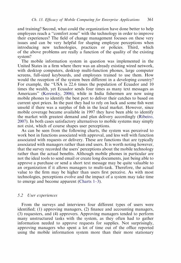
and training? Second, what could the organization have done better to helpemployees reach a ‘‘comfort zone’’ with the technology in order to improvetheir experiences? The field of change management focuses on these veryissues and can be very helpful for shaping employee perceptions whenintroducing new technologies, practices or policies. Third, whichof the above problems are really a function of the quality of the existingsystem?The mobile information system in question was implemented in the
United States in a firm where there was an already existing wired network,with desktop computers, desktop multi-function phones, large computerscreens, full-sized keyboards, and employees trained to use them. Howwould the reception of the system been different in a developing country?For example, the ‘‘USA is 22.6 times the population of Ecuador and 10times the wealth, yet Ecuador sends four times as many text messages asAmericans’’ (Kerensky, 2006), while in India fishermen are now usingmobile phones to identify the best port to deliver their catches to based oncurrent spot prices. In the past they had to rely on luck and some fish wentunsold if there was a surplus of fish in the local market. However, sincemobile coverage became available in 1997 they have been able to identifythe market with greatest demand and plan delivery accordingly (Ribeiro,2007). In both cases satisfactory alternatives to mobile systems may simplynot exist, which of course shapes user perceptions.As can be seen from the following charts, the system was perceived to
work best in functions associated with approval, and less well with functionassociated with requests or delivery. These are functions that are typicallyassociated with managers rather than end users. It is worth noting however,that the survey recorded the users’ perceptions about the mobile technologyrather than the actual benefits. Although mobile phones in particular arenot the ideal tools to send email or create long documents, just being able toapprove a purchase or send a short text message may be quite valuable toan organization if it allows managers to multi-task. Therefore, the actualvalue to the firm may be higher than users first perceive. As with mosttechnologies, perceptions evolve and the impact of a system may take timeto emerge and become apparent (Charts 1–3).
5.2 User experiences
From the surveys and interviews four different types of users wereidentified; (1) approving managers, (2) finance and accounting managers,(3) requesters, and (4) approvers. Approving managers tended to performmany unstructured tasks with the system, as they often had to gatherinformation needed to approve requests for supplies. Not surprisingly,approving managers who spent a lot of time out of the office reportedusing the mobile information system more than their more stationary
Ch. 13. Efficacy of Mobile Computing for Enterprise Applications 361

counterparts, and generally they found the system useful (see Chart 2).However, some approving managers were so overwhelmed by the frequentuse of the notification feature that they eventually disabled it. This mayindicate that there are still problems regarding how business processes arestructured.In contrast, finance and accounting managers tended to use the system
for more routine tasks that usually involved following simple business rules,i.e. checking to make sure requisitions were within budgetary limits. Thesemanagers used the system for mainly communication purposes and to
0
10
20
30
40
50
60
70
80
Notification aboutwaiting approval
requests
Delegation ofapproval authority
Interpersonalcommunication
Access toadditional dataduring approval
Approval ofpurchase orders
Support of Mobile Business Applications for Different Procurement Activities
%
Extent to which mobile business applications can provide support for approvals (% of all occurrences that can be supported)
Chart 2. Approvals.
0
10
20
30
40
50
60
70
80
Select items fromcatalog
Submit purchasingrequest
Track purchaseorder
Change purchaseorder
Cancel purchaseorder
Support of Mobile Business Applications for Different Procurement Activities
%
Extent to which mobile business applications can provide support for requests(% of all occurrences that can be supported)
Chart 1. Requests.
John Burke et al.362
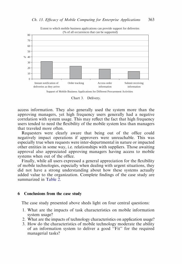
access information. They also generally used the system more than theapproving managers, yet high frequency users generally had a negativecorrelation with system usage. This may reflect the fact that high frequencyusers tended to need the flexibility of the mobile system less than managersthat traveled more often.Requesters were clearly aware that being out of the office could
negatively impact operations if approvers were unreachable. This wasespecially true when requests were inter-departmental in nature or impactedother entities in some way, i.e. relationships with suppliers. Those awaitingapproval also appreciated approving managers having access to mobilesystems when out of the office.Finally, while all users expressed a general appreciation for the flexibility
of mobile technologies, especially when dealing with urgent situations, theydid not have a strong understanding about how these systems actuallyadded value to the organization. Complete findings of the case study aresummarized in Table 2.
6 Conclusions from the case study
The case study presented above sheds light on four central questions:
1. What are the impacts of task characteristics on mobile informationsystem usage?
2. What are the impacts of technology characteristics on application usage?3. How do the characteristics of mobile technology moderate the ability
of an information system to deliver a good ‘‘Fit’’ for the requiredmanagerial tasks?
0
10
20
30
40
50
60
70
80
Instant notification ofdeliveries as they arrive
Order trackinginformation
Submit receivinginformation
Support of Mobile Business Applications for Different Procurement Activities
%
Access order
Extent to which mobile business applications can provide support for deliveries (% of all occurrences that can be supported)
Chart 3. Delivery.
Ch. 13. Efficacy of Mobile Computing for Enterprise Applications 363

Table 2
Research propositions and evidence from case study
Case study results
Research framework
construct
Proposition Evidence from case
study?
Finding
Functionality 1. Users will first use mobile business
applications for notification and
communication purposes rather than for
data processing or information access
Limited Users showed willingness to use mobile devices
(cell phones) for ‘‘innovative’’ purposes
Portability 2. There is a tradeoff between portability and
usability of mobile devices, effectively
limiting the usage of mobile business
applications to simple activities
Yes Factor will become less significant in the future
as improved mobile devices become available
System performance
and user support
3. System performance and user support have
a positive impact on the usage of mobile
business applications
Yes (strong evidence) Strong evidence for the need to make the effort
‘‘worthwhile’’; poor performance can have a
detrimental effect on usage
Task structure 4a. Employees performing highly structured
tasks tend to use mobile business
applications for data processing
Yes
4b. Employees performing unstructured tasks
tend to use mobile business applications to
access information and for communication
purposes
JohnBurkeet
al.
364
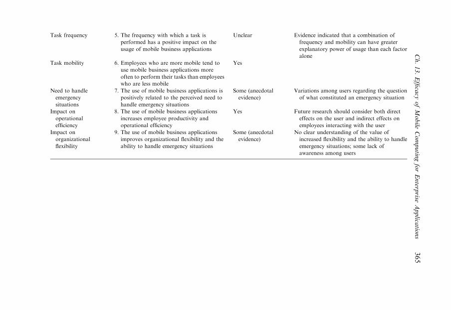
Task frequency 5. The frequency with which a task is
performed has a positive impact on the
usage of mobile business applications
Unclear Evidence indicated that a combination of
frequency and mobility can have greater
explanatory power of usage than each factor
alone
Task mobility 6. Employees who are more mobile tend to
use mobile business applications more
often to perform their tasks than employees
who are less mobile
Yes
Need to handle
emergency
situations
7. The use of mobile business applications is
positively related to the perceived need to
handle emergency situations
Some (anecdotal
evidence)
Variations among users regarding the question
of what constituted an emergency situation
Impact on
operational
efficiency
8. The use of mobile business applications
increases employee productivity and
operational efficiency
Yes Future research should consider both direct
effects on the user and indirect effects on
employees interacting with the user
Impact on
organizational
flexibility
9. The use of mobile business applications
improves organizational flexibility and the
ability to handle emergency situations
Some (anecdotal
evidence)
No clear understanding of the value of
increased flexibility and the ability to handle
emergency situations; some lack of
awareness among users
Ch.13.Efficacy
ofMobile
Computin
gforEnterp
riseApplica
tions
365

4. What is the impact on usage of mobile information systems onbusiness processes?
In respect to the first question the study found that users valuednotification and support for simple tasks like tracking orders most highly asopposed to handling more complex operations. However, access to ad hocinformation was also highly valued. This was especially true for managerswho were highly mobile and had a need to process urgent requests while onthe move between locations for meetings, etc. Therefore as expected,managers who were often ‘‘wandering’’ valued the smart phone mobileapplication system the most.In respect to the second question, the study found that poor technology
characteristics like phones with small screens and keyboards inhibitedusage. Also, some employees did not like carrying around the encryptionkey that was used to log into the system from mobile devices, while othersnoted that training and support were key issues that limited their usage ofthe mobile information system.For the third question, it appears that how the mobile technology
affected the organization very much depended on the kind of user involved.Approving managers valued the system more than accounting and financestaff largely because they were more mobile and thus had more incentive tolearn and use the new system. Also, the system did greatly increase theefficiency and processing speed of the requisition system since it allowedusers to access the system in situations when they previously would havebeen simply ‘‘out of the office’’. This in turn allowed users who depended onapproval of their requests to do their own jobs more efficiently. However,while most employees recognized the potential benefits of the system,reactions were in fact mixed. While many expected mobile technology toadd additional flexibility to the organization, others questioned the strategicvalue of making the procurement function mobile. This was especially truefor finance and accounting managers who were basically stationary.As far as the overall conclusions that can be drawn from the case
regarding the impact of mobile technology on business processes, it wasclear that users had high expectations. They were impatient withconnectivity problems, and frustrated by hardware limitations such assmall screens and keyboards. While many employees recognized thepotential benefits in efficiency that could be realized by the organization,many expressed skepticism about using it in this instance. Even moreinteresting, one employee mentioned simply turning off the mobile devicebecause they were overwhelmed with the number of requests that weredirected to them. This perhaps indicates that more needs to be done on:
� Improving the fit between the devices chosen and the tasks they need toperform.� Improving the fit between the devices provided and the users that usethem, (i.e. giving wanderers smart phones and stationary users desktops).
John Burke et al.366

� Identifying the appropriate scope of a system. Does the system reallyneed to be department-wide or should the system be limited to asmaller subset of users to maximize impact.� Increasing the training of the users, so that they know how to use thesystem and so that they understand the importance of the system to theorganization.� Educating the users on the strengths and weaknesses of mobile systemsin advance of deployment, in order to avoid unrealistic expectations.If users’ expectations can be set in advance, less frustration shouldresult from the technology’s inherent characteristics and limitations.� Managing user perceptions over time through ‘‘change management’’techniques. As noted several times perceptions are not static. What canan organization do to so that user experiences evolve in a positive way?What can management do before, during and after implementation toimprove system success?� Measuring the value of a system as well as the perception of value isalso important. For example, if a manager uses a mobile system onlywhile they are on the run and under stress they may not fullyappreciate the system’s value simply because they do not realize howmuch time the system saved them.� Modifying the business rules and processes as appropriate so that usersare not overwhelmed by the new technology. Technology cannot helpthe organization if employees turn it off!
7 New research opportunities
The case study presented points to a few areas of research, both academicand practical that need to be explored. On the academic side a variety ofresearch questions present themselves.
� How can organizations design mobile devices and services so that theyare easy for individuals to use and understand?� How can mobile technology be used to support teams of employees,rather than just single users?� How will the advent of ubiquitous computing affect the structure oforganizations?� What are the security implications of ubiquitous computing, especiallygiven government privacy regulations?� How will organizations have to change their infrastructures toseamlessly support heterogeneous data across heterogeneous devices?What types of protocols and standards need to be developed beforeubiquitous computing can be supported?� How do business processes have to change, as ubiquitous computingbecomes a reality?
Ch. 13. Efficacy of Mobile Computing for Enterprise Applications 367

On the practical side, first it is clear that mobile devices are quicklyreaching a level of technical maturity where they can start to replace manytraditional non-mobile systems. However, as was clear from the case manypractical issues remain.
� What kind of users does a firm have, wanderers, travelers, or visitors?� What kind of devices should a firm purchase and how can they beintegrated?� How can firms train their employees to use mobile systems mosteffectively?� How should firms decide which applications should be made mobileapplications? Do these applications justify the cost?
8 Conclusion
Most of the discussion above including the case study focused onusing mobile technology to improve the efficiency of existing processesand corporate structures. However, an equally important question ishow will these new devices and systems change business processes in thefuture?Five hundred years ago most organizations had very few employees,
existed for a very limited time, sometimes only for one day, and usually onlyin one place. In such cases, very little effort was needed to control orcommunicate to workers, and voice communication usually sufficed.However, over time organizations have grown to the point where todaythey may span several countries, have tens of thousands of employees usingseveral languages, and require worldwide communication systems that usedifferent technologies at the same time. This trend towards increasingcomplexity can be expected to continue, especially if one considers thebroader organization including suppliers, outsourcing vendors, and down-stream customers.Therefore, managers are now realizing that mobile technologies offer the
potential for organizations to connect all of their employees, customers,managers, suppliers, and partners just as consumer devices like cell phonesare connecting families. However, the wide scope that mobile informationsystems encompass can itself become a problem. Especially when systemscross international, corporate, divisional, or vendor lines devices tend tobecome heterogeneous.Although the issue was not actively explored above, one major issue that
was faced by the company was which mobile device(s) should be theplatform for its procurement system. PDA’s, Smart phones and laptopswere all potential devices, and several vendors and models were identified.Devices that had large keyboards and screens were easier for some users,
John Burke et al.368

particularly for those that needed to use the system a lot, but were relativelystationary. Managers that needed to wander a lot obviously preferredsmaller devices that were easier to carry. Unfortunately these devices werenot completely compatible and this contributed to difficulties in providinguser support. How organizations connect and manage the multitude ofdevices from different vendors is a real issue that executives actively need toaddress both technically and culturally.Technically, devices in the future will likely need to be able to adapt to
new situations through the use of dynamically deployed processes andsystems, such as through the use of the SATIN component system(Zachariadis et al., 2006). This system proposes that as users move fromplace to place their devices would be actively updated with the appropriatecode (ideally using cross platform code components), appropriate to theirnew location largely automatically. Much like users today download newring tones, future systems will need to intelligently download appropriateapplications or add-ons to existing applications. Cultural barriers may evenpresent greater technical problems. How do you adapt a phone designed forthe USA to the Cyrillic character set if the user suddenly travels to Russia,and how do you design a Smart phone with a large keyboard and screenthat is still fashionable enough for use in Hong Kong?Furthermore, new government regulations regarding information privacy
and the tracking of hazardous materials require greater integration withinsupply chains, and some firms are looking to mobile technologies to helptheir companies stay within compliance. How these different forces willaffect mobile technologies has yet to be determined.Another interesting issue that is illustrated by the case study is that
perhaps a new perspective is needed when designing systems. For the last 50years technology has often been used to increase the efficiency of existingsystems. Accounting systems, resource management systems, database anddocument processing systems have all been automated through technology.However, as was seen in the case study, it is not necessarily sufficient tosimply add new technology to existing systems without rethinking thebusiness processes. In the procurement system described above it is clearthat managers that were often out of the office liked the system, whereasmost users found it difficult to use. In a sense the system was designed withmanagers in mind rather than with the users who would actually requestitems.Given the increase in power and portability of new devices it may be time
to rethink business processes entirely and focus on the end user. While thisis an often-stated idea, the reality is that most automated accountingsystems and enterprise resource planning systems focus on reducing costsrather than on improving usability. Put another way, systems are oftendesigned for the convenience of the enterprise rather than for the actualusers of the system whether employees or customers.
Ch. 13. Efficacy of Mobile Computing for Enterprise Applications 369

Example of how technology can have unexpected negative consequences
There are several local hospitals that serve the University of Illinois atUrbana-Champaign. One in particular, has a very modern mobileinformation system that allows doctors to wirelessly enter the results ofexaminations and medical tests directly into the hospitals records systemusing laptops. The doctors can also use the wireless system to send mostprescriptions to a variety of local pharmacies while still moving fromroom to room. It is a very convenient system for the doctors.When patients want to find out the results of their medical tests they
can simply call the appropriate medical office and in theory a nurse canlook up the information on the system right away. Unfortunatelymedical offices are busy places and nurses are often with patients. It maytake several calls to the office being placed on hold for 10–15min at atime before a nurse is available to look up the necessary information,especially if the doctor has not fully updated the patient’s records. In thiscase, the nurse has to track down the doctor all the while the patient iswaiting on hold. It is a system that many readers are probably familiarwith, and in the days of wired phones it worked satisfactorily.However, this system does not work well for those, like students, who
use mobile technology themselves and have cell phone plans that havelimited anytime minutes. They simply cannot afford to wait on hold for30min. Even if they have unlimited night and weekend minutes hospitaloffices are generally not open on nights and weekends. The result, it isoften easier to drive to the hospital to get the information than to call!This is a clear example where the switch from traditional to mobiletechnology, by the customer in this case, has caused a marked drop incustomer service.This illustrates the need to always consider your customer when
designing your system. Does the hospital’s system really end with thedoctors and nurses? Obviously not, so while the bulk of this chapterconcerned a mobile information system that was internal to anorganization, it is important to always remember to ask how do anorganization’s information systems ultimately affect the customer? Thehospital system freed doctors and nurses to wander away from theiroffices, but ultimately also limited the ability of patients to tract themdown as well!
References
Angeles, R. (2005). RFID technologies: supply-chain applications and implementation issues.
Information Systems Management 22(1), 51–65.
Bostrom, R., J.S. Heinen (1977). MIS problems and failures: a socio-technical perspective. MIS
Quarterly 1(3), 17–32.
John Burke et al.370
Davis, F. (1989). Perceived usefulness, perceived ease of use, and user acceptance of information
technology. MIS Quarterly 13(3), 319–340.
Dishaw, M.T., D.M. Strong (1998). Supporting software maintenance with software engineering tools: a
computed task-technology fit analysis. Journal of Systems and Software 44(2), 107–120.
Dishaw, M.T., D.M. Strong (1999). Extending the technology acceptance model with task-technology fit
constructs. Information & Management 36(1), 9–21.
Gebauer, J., M. Shaw (2002). A Theory of Task/Technology Fit for Mobile Applications to Support
Organizational Processes. College of Business Working Paper CITEBM-02–03, University of Illinois
at Urbana-Champaign.
Gebauer, J., M. Shaw (2004). Success factors and benefits of mobile business applications: results from a
mobile E-procurement study. International Journal of Electronic Commerce 8(3), 19–41.
Gebauer, J., M.J. Shaw, M.L. Gribbins (2005). Task-Technology Fit for Mobile Information Systems.
College of Business Working Paper 05-0119.
Goodhue, D.L., R.L. Thompson (1995). Task-technology fit and individual performance. MIS
Quarterly 19(2), 213–236.
Kerensky, L. (2006). For Better or for Worse, Mobile is on the Move. Adotas.com. Available at http://
www.adotas.com/2006/08/for-better-or-for-worse-mobile-is-on-the-move/. Current June 29, 2007.
Lyytinen, K., Y. Yoo (2002a). Research commentary: the next wave of nomadic computing. Information
Systems Research 45(12), 63–65.
Lyytinen, K., Y. Yoo (2002b). Issues and challenges in ubiquitous computing. Communications of the
ACM 13(4), 377–388.
Milgram, S. (1967). The small world problem. Psychology Today 2, 60–67.
Ribeiro, J. (2007). To do with the price of fish. Economist.com. Available at http://www.economist.com/
finance/displaystory.cfm?story_id ¼ 9149142. Current June 29, 2007.
Sarker, S., J.D. Wells (2003). Understanding mobile handheld device use and adoption. Communications
of the ACM 46(12), 35–40.
Venkatesh, V., M.G. Morris, G.B. Davis, F.D. Davis (2003). User acceptance of information
technology: toward a unified view. MIS Quarterly 27(3), 425–478.
Zachariadis, S., C. Mascolo, W. Emmerich (2006). The SATIN component system—A metamodel for
engineering adaptable mobile systems. IEEE Transactions on Software Engineering 32(11), 910–927.
Zigurs, I., B.K. Buckland (1998). A theory of task-technology fit and group support system
effectiveness. MIS Quarterly 22(3), 313–334.
Zigurs, I., B.K. Buckland, J.R. Connolly, E.V. Wilson (1999). A test of task/technology fit theory for
group support systems. Database for Advances in Information Systems 30(3/4), 34–50.
Ch. 13. Efficacy of Mobile Computing for Enterprise Applications 371

This page intentionally left blank

Adomavicius & Gupta, Eds., Handbooks in Information Systems, Vol. 3
Copyright r 2009 by Emerald Group Publishing Limited
Chapter 14
Web-Based Business Intelligence Systems:A Review and Case Studies
Wingyan ChungDepartment of Operations and Management Information Systems, Leavey School of Business,
Santa Clara University, Santa Clara, CA 95053, USA
Hsinchun ChenDepartment of Management Information Systems, Eller College of Management, The University of
Arizona, Tucson, AZ 85721, USA
Abstract
As businesses increasingly use the Web to share and disseminate information,effectively and efficiently discovering business intelligence (BI) fromvoluminous information has challenged researchers and practitioners. Inthis chapter, we review literature in BI on the Web and technology for Webanalysis, and propose a framework for developing Web-based BI systems,which can help managers and analysts to understand their competitiveenvironment and to support decision-making. The framework consists ofsteps including collection, conversion, extraction, analysis, and visualizationthat transform Web data into BI. Combinations of data and text mining(TM) techniques were used to assist human analysis in different scenarios.We present three case studies applying the framework to BI discovery on theWeb. In these studies, we designed, developed, and evaluated Web-based BIsystems that search for and explore BI from a large number of Web pagesand help analysts to classify and visualize the results. Experimental resultsshow that the systems compared favorably with benchmark methods,showing the usability of the framework in alleviating information overloadand in collecting and analyzing BI on the Web. Considering the scarceresearch work found in this field, this chapter provides valuable insights andnew research findings on developing Web-based BI systems. Futuredirections of BI research are discussed.
373

1 Introduction
As businesses increasingly share and disseminate information on theWeb, information overload often hinders discovery of business intelligence(BI). A study found that the world produces between 3.41 million and 5.61million terabytes of unique information per year, most of which has beenstored in computer hard drives or servers (Lyman and Varian, 2003). Manyof these computing devices serve as the repository of the Internet,supporting convenient access of information but also posing challengesof effective knowledge discovery from voluminous information. Suchconvenient storage of information on the Web has made informationexploration difficult (Bowman et al., 1994). While it is easy to access a largenumber of Web repositories nowadays, it is difficult to identify therelationships among interconnected Web resources. A study found thatover 90% of pages on the public Web are connected to other Web pagesthrough hyperlinks (Broder et al., 2000). The proliferation of electroniccommerce further aggravates the problems of identifying business relation-ships on the Web. Business managers and analysts need better approachesto understand large amounts of information and data. Effectively andefficiently discovering BI from vast amount of information on the Web thushas challenged researchers and practitioners. Unfortunately, little researchon BI systems and applications has been found in the literature (Negash,2004).This chapter reviews related work on BI systems and mining the Web for
BI, describes a framework for discovering BI on the Web, and presentsthree case studies applying the framework to designing and developingWeb-based BI systems, which can help managers and analysts to under-stand their competitive environment and to support decision-making. Ourpurpose is to inform the community of researchers and practitioners aboutrecent advances in BI research and to enrich this still young field.
2 Literature review
BI is defined as the product of systematic acquisition, collation, analysis,interpretation, and exploitation of business information (Chung et al.,2005). As the Web becomes a major source of business information(Futures-Group, 1998), Web-based BI emerges to be a valuable resource formanagers to understand the business environment, to devise competitivestrategies, and to support decision-making. For example, businessmanagers and analysts can study competitors’ movements by analyzingtheir Web site content and hyperlinks. Web log messages, news articles, andonline forum messages can be analyzed to extract customer preferences oremerging trends. We review below literature on BI systems and Web mining
W. Chung and H. Chen374

technologies. Our scope of review is on analyzing and extracting Web-basedBI from organizations’ external environment.
2.1 Business intelligence systems
BI systems enable organizations to understand their internal and externalenvironments. Two classes of BI tools have been defined (Carvalho andFerreira, 2001). The first class of these is used to manipulate massiveoperational data and to extract essential business information from acompany’s (internal) operational data. Examples include decision supportsystems, executive information systems, online-analytical processing(OLAP), data warehouses and data mining systems that are built upondatabase management systems to reveal hidden trends and patterns (Choo,1998). The second class of BI tools, sometimes called competitiveintelligence (CI) tools, aims at systematically collecting and analyzinginformation from the external business environment to assist in organiza-tional decision-making. They mainly gather information from publicsources such as the Web. Rooted in military strategy (Cronin, 2000;Nolan, 1999), these BI tools also provide insights into various value-addingprocesses in knowledge discovery. In contrast to the first class of BI tools,technologies for collecting and analyzing data from external environmentare less standardized due to the relatively unstructured nature of the data.These technologies have to implement the steps in the BI discovery process.
2.1.1 BI discovery processResearchers have proposed various steps in the process of discovering BI.
Taylor proposes a value-added spectrum consisting of four major phases:organizing processes (grouping, classifying, relating, formatting, signaling,displaying); analyzing processes (separating, evaluating, validating, com-paring, interpreting, synthesizing); judgmental processes (presentingoptions, presenting advantages, presenting disadvantages), and decisionprocesses (matching goals, compromising, bargaining, choosing) (Taylor,1986). Some authors add ‘‘evaluation’’ as a feedback loop (Fuld et al.,2002). Through the different phases, transformations take place in the orderof data, information, informing knowledge, productive knowledge, andaction. The difficulty to discover BI increases as one progresses along thephases because data are less structured and requires more processing.An empirical study of BI implementation helps to identify four phases
(Westney and Ghoshal, 1994) similar to Taylor’s spectrum. The datamanagement phase consists of acquisition, classification, storage, retrieval,editing, verification and quality control, presentation, aggregation,distribution, and assessment. The analysis phase consists of synthesis,hypothesis, and assumption building and testing. The implication and
Ch.14. Web-Based Business Intelligence Systems 375

action phases, respectively, concern how analysts should respond and whattasks should be performed.
2.1.2 Commercial BI toolsFuld et al. (2003) found that the global interest in BI technology has
increased significantly over the past five years. They compared 16commercial BI tools based on a 5-stage intelligence cycle: (1) planningand direction, (2) published information collection, (3) source collectionfrom humans, (4) analysis, and (5) reporting and information sharing.It was found that the tools have become more open to the Web, throughwhich businesses nowadays share information and perform transactions.There is no ‘‘one-size-fits-all solution’’ because different tools are used fordifferent purposes.In terms of the weaknesses of BI tools, automated search capability in
many tools can lead to information overload. Despite improvements inanalysis capability over the past year (Fuld et al., 2002), there is still a longway to go to assist qualitative analysis effectively. Most tools that claim todo analysis simply provide different views of collection of information (e.g.,comparison between different products or companies). More advancedtools use text mining (TM) technology or rule-based systems to determinerelationships among people, places, and organizations using a user-defineddictionary or dynamically generated semantic taxonomy. Because existingBI tools are not capable of illustrating the landscape of a large numberof documents collected from the Web, their actual value to analysis isquestionable (Fuld et al., 2003). In addition, only few improvements havebeen made to reporting and information sharing functions, although manytools integrate their reports with Microsoft Office products and presentthem in a textual format.
2.2 Mining the Web for BI
As most resources on the Web are text-based, automated tools andtechniques have been developed to exploit textual information. Forinstance, Fuld et al. (2003) have noticed that more BI tools are nowcompatible with the Web than in the past. Although text expresses a vast,rich range of information, it encodes this information in a form that isdifficult to decipher automatically (Hearst, 1999), to which researchers haverecently identified TM as a potential solution. Compared with data mining,TM focuses on knowledge discovery in textual documents and involvesmultiple processes.
2.2.1 Text miningTM is the process of finding interesting or useful patterns in textual data
and information. An example is analyzing textual descriptions in financial
W. Chung and H. Chen376
news to predict stock market movements. TM combines many of thetechniques of information extraction, information retrieval, naturallanguage processing, and document summarization (Hearst, 1999; Trybula,1999). It provides a means of developing knowledge links and knowledgesharing among people within organizations. Though the field is in itsinfancy, it has been anticipated to have explosive growth in order to addressgrowing information challenges in organizations (Trybula, 1999). TMevolved from the field of automatic text processing that emerged in the1970s, and was influenced by related fields of machine learning in the 1980s,and data mining, knowledge discovery, and Web mining in the 1990s.In recent years, businesses increasingly rely on TM to discover intelligenceon the Web.Trybula (1999) proposes a framework for knowledge discernment in text
documents. The framework includes several processes to transform textualdata into knowledge: (1) Information acquisition: The text is gatheredfrom textbases at various sources, through finding, gathering, cleaning,transforming, and organizing. Manuscripts are compiled into a prepro-cessed textbase. (2) Extraction: The purpose of extraction is to provide ameans of categorizing the information so that relationships can beidentified. Activities include language identification, feature extraction,lexical analysis, syntactic evaluation, and semantic analysis. (3) Mining: Itinvolves clustering in order to provide a manageable size of textbase relation-ships that can be evaluated during information searches. (4) Presentation:Visualizations or textual summarizations are used to facilitate browsing andknowledge discovery.Although Trybula’s framework covers important areas of TM, it has
several limitations for TM on the Web. First, there needs to be morepreprocessing of documents on the Web, because they exist in manyformats such as HTML, XML, and dynamically generated Web pages.Second, efficient and effective methods are needed to collect Web pagesbecause they are often voluminous. Human collection does not scale tothe growth of the Web. Third, information on the Web comes fromheterogeneous sources and requires better integration and more discrimina-tion. Fourth, more mining and visualization options other than clusteringare needed to reveal hidden patterns in noisy Web data. Web miningtechnologies are needed to augment TM for discovering BI.
2.2.2 Web miningWeb mining is the use of data mining techniques to automatically
discover and extract information from Web documents and services(Etzioni, 1996). Machine learning techniques have been applied to Webmining (Chen and Chau, 2004). Given the exponential growth of the Web,it is difficult for any single search engine to provide comprehensive coverageof search results. Meta-searching has been shown to be a highly effectivemethod of resource discovery and collection on the Web. By sending
Ch.14. Web-Based Business Intelligence Systems 377
queries to multiple search engines and collating the set of top-ranked resultsfrom each search engine, meta-search engines can greatly reduce bias insearch results and improve coverage. Chen et al. (2001) showed that theapproach of integrating meta-searching with textual clustering toolsachieved high precision in searching the Web.To extract information and uncover patterns from Web pages or sites,
three categories of Web mining have been identified: Web content mining,Web structure mining, and Web usage mining (Kosala and Blockeel, 2000).Web content mining refers to the discovery of useful information from Webcontents, such as text, image, video, audio, and so on. Previous work onWeb content mining include Web-page categorization (Chen et al., 1996),clustering (Zamir and Etzioni, 1999), rule and pattern extraction (Hurst,2001), and concept retrieval (Chen et al., 1998; Schatz, 2002). Web structuremining refers to the analysis of link structures that model the Web,encompassing work on resource discovery (Chakrabarti et al., 1999), Web-page ranking (Brin and Page, 1998; Lempel and Moran, 2001), authorityidentification (Kleinberg, 1999; Mendelzon and Rafiei, 2000), and evolutionof the Web documents (Henzinger and Lawrence, 2004). Web usage miningstudies techniques that can predict user behavior while the user interactswith the Web. Knowledge of Web usage can contribute to buildinge-commerce recommender systems (Pazzani, 1999), Web-based personali-zation and collaboration (Adomavicius and Tuzhilin, 2001), and decisionsupport (Chen and Cooper, 2001).In addition to the aforementioned Web mining technologies, there have
been applications of machine learning and data mining techniques to Webmining. Web-page summarization, a process of automatically generating acompact representation of a Web page based on the page features and theirrelative importance (Hearst, 1994; McDonald and Chen, 2002), can be usedto facilitate understanding of search engine results. Web-page classification,a process of automatically assigning Web pages into predefined categories,can be used to assign pages into meaningful classes (Mladenic, 1998). Web-page clustering, a process of identifying naturally occurring subgroupsamong a set of Web pages, can be used to discover trends and patternswithin a large number of pages (Chen et al., 1996). Web-page visualization,a process of transforming a high-dimensional representation of a set of Webpages into a two- or three-dimensional representation that can be perceivedby human eyes, can be used to represent important knowledge as pictures(Yang et al., 2003).
3 A framework for discovering BI on the Web
Although a number of data and TM technologies exist, there has not yetbeen a comprehensive framework to address problems of discovering BI onthe Web. Data and TM technologies hold the promise for alleviating these
W. Chung and H. Chen378
problems by augmenting human analysis. However, applying thesetechnologies effectively requires consideration of several factors related tothe Web itself, such as the use of collection methods, Web-page parsing andinformation extraction, the presence of hyperlinks, and language differencesin heterogeneous information sources. Unfortunately, existing frameworksusing data and TM techniques (e.g., Nasukawa and Nagano, 2001; Soper,2005; Trybula, 1999) do not address these issues. Research on intelligentWeb technologies (e.g., Zhong et al., 2003) seldom addresses the need for BIdiscovery on the Web (Negash, 2004).To address the needs, we have developed a framework for discovering BI
on the Web. The rationale underlying our framework is to capture strengthsof different data and TM techniques and to complement their weaknesses,thereby effectively assisting human analysts as they tackle problems ofdiscovering BI on the Web. As shown in Fig. 1, the framework providessystem designers useful tools, techniques, and guidelines to design anddevelop Web-based BI systems.The framework consists of five steps: collection, conversion, extraction,
analysis, and visualization. Input to and output from the framework are,respectively, Web data and BI discovered after applying the steps. Each stepallows human knowledge to guide the application of techniques (e.g.,heuristics for parsing, weighting in calculating similarities, keywords formeta-searching/meta-spidering). The steps shown in Fig. 1 are collections ofprocessed results: Web pages and documents; a tagged collection; indexesand relationships; similarities, classes, and clusters; and hierarchies, maps,and graphs. As we move from left to right of these collections, the degree ofcontext and difficulty to detect noise in the results increase. The three left-hand-side collections are labeled ‘‘data and text bases’’ and the two right-hand-side collections are labeled ‘‘knowledge bases.’’ The former mainlycontain raw data and processed textual information while the latter containBI discovered from data and text bases. We explain each step in thefollowing sections.
3.1 Collection
The purpose of this step is to acquire raw data for creating research testbeds. Data in the forms of textual Web pages (e.g., HTML, XML, JSP,ASP, etc.) are collected. Several types of data are found in these pages:textual content (the text that can be seen on an Internet browser),hyperlinks (embedded behind anchor text), and structural content (textualmark-up tags that indicate the types of content on the pages).To collect these data, meta-searching/meta-spidering and domain
spidering are used.Meta-spidering is an enhanced version of meta-searchingusing keywords as inputs. These keywords can be identified by humanexperts or by reviewing related literature. In addition to obtaining results
Ch.14. Web-Based Business Intelligence Systems 379
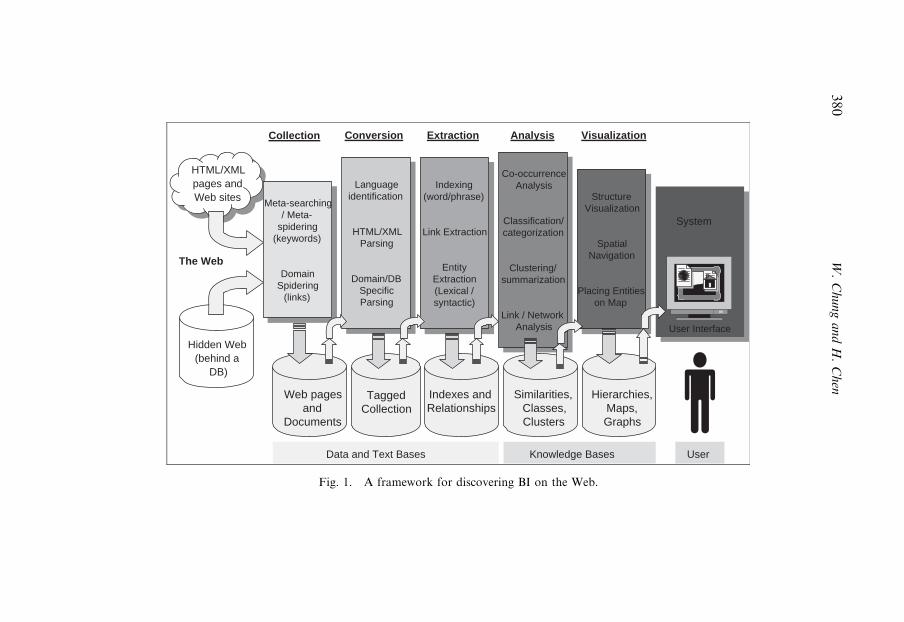
System
User Interface
System
User Interface
Knowledge Bases
Language identification
HTML/XML Parsing
Domain/DB Specific Parsing
Language identification
HTML/XML Parsing
Domain/DB Specific Parsing
Tagged Collection
Indexes and Relationships
Similarities, Classes,Clusters
Web pages and
Documents
Hierarchies, Maps, Graphs
Collection Conversion Extraction Analysis Visualization
Indexing (word/phrase)
Link Extraction
Entity Extraction (Lexical / syntactic)
Indexing (word/phrase)
Link Extraction
Entity Extraction (Lexical / syntactic)
Co-occurrence Analysis
Classification/ categorization
Clustering/ summarization
Link / Network Analysis
Co-occurrence Analysis
Classification/ categorization
Clustering/ summarization
Link / Network Analysis
Structure Visualization
Spatial Navigation
Placing Entities on Map
Structure Visualization
Spatial Navigation
Placing Entities on Map
The Web
Hidden Web (behind a
DB)
HTML/XML pages and Web sites
Meta-searching / Meta-
spidering (keywords)
Domain Spidering
(links)
Meta-searching / Meta-
spidering (keywords)
Domain Spidering
(links)
Data and Text Bases User
Fig. 1. A framework for discovering BI on the Web.
W.ChungandH.Chen
380
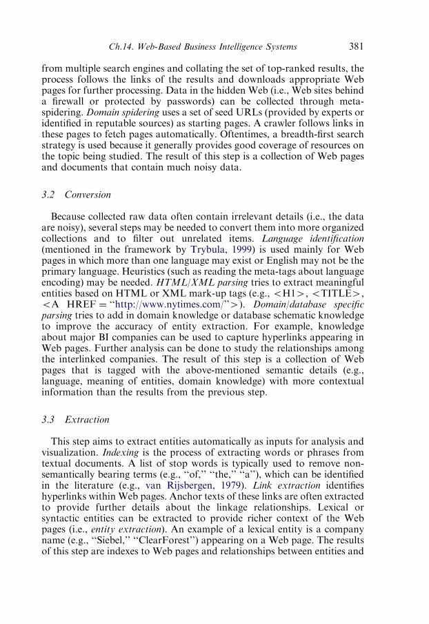
from multiple search engines and collating the set of top-ranked results, theprocess follows the links of the results and downloads appropriate Webpages for further processing. Data in the hidden Web (i.e., Web sites behinda firewall or protected by passwords) can be collected through meta-spidering. Domain spidering uses a set of seed URLs (provided by experts oridentified in reputable sources) as starting pages. A crawler follows links inthese pages to fetch pages automatically. Oftentimes, a breadth-first searchstrategy is used because it generally provides good coverage of resources onthe topic being studied. The result of this step is a collection of Web pagesand documents that contain much noisy data.
3.2 Conversion
Because collected raw data often contain irrelevant details (i.e., the dataare noisy), several steps may be needed to convert them into more organizedcollections and to filter out unrelated items. Language identification(mentioned in the framework by Trybula, 1999) is used mainly for Webpages in which more than one language may exist or English may not be theprimary language. Heuristics (such as reading the meta-tags about languageencoding) may be needed. HTML/XML parsing tries to extract meaningfulentities based on HTML or XML mark-up tags (e.g., oH1W, oTITLEW,oA HREF ¼ ‘‘http://www.nytimes.com/’’W). Domain/database specificparsing tries to add in domain knowledge or database schematic knowledgeto improve the accuracy of entity extraction. For example, knowledgeabout major BI companies can be used to capture hyperlinks appearing inWeb pages. Further analysis can be done to study the relationships amongthe interlinked companies. The result of this step is a collection of Webpages that is tagged with the above-mentioned semantic details (e.g.,language, meaning of entities, domain knowledge) with more contextualinformation than the results from the previous step.
3.3 Extraction
This step aims to extract entities automatically as inputs for analysis andvisualization. Indexing is the process of extracting words or phrases fromtextual documents. A list of stop words is typically used to remove non-semantically bearing terms (e.g., ‘‘of,’’ ‘‘the,’’ ‘‘a’’), which can be identifiedin the literature (e.g., van Rijsbergen, 1979). Link extraction identifieshyperlinks within Web pages. Anchor texts of these links are often extractedto provide further details about the linkage relationships. Lexical orsyntactic entities can be extracted to provide richer context of the Webpages (i.e., entity extraction). An example of a lexical entity is a companyname (e.g., ‘‘Siebel,’’ ‘‘ClearForest’’) appearing on a Web page. The resultsof this step are indexes to Web pages and relationships between entities and
Ch.14. Web-Based Business Intelligence Systems 381
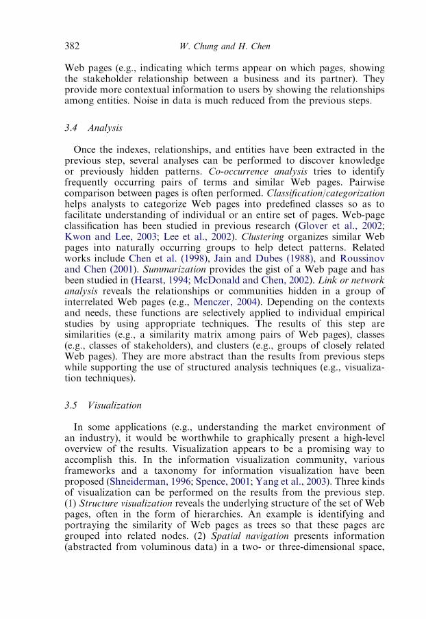
Web pages (e.g., indicating which terms appear on which pages, showingthe stakeholder relationship between a business and its partner). Theyprovide more contextual information to users by showing the relationshipsamong entities. Noise in data is much reduced from the previous steps.
3.4 Analysis
Once the indexes, relationships, and entities have been extracted in theprevious step, several analyses can be performed to discover knowledgeor previously hidden patterns. Co-occurrence analysis tries to identifyfrequently occurring pairs of terms and similar Web pages. Pairwisecomparison between pages is often performed. Classification/categorizationhelps analysts to categorize Web pages into predefined classes so as tofacilitate understanding of individual or an entire set of pages. Web-pageclassification has been studied in previous research (Glover et al., 2002;Kwon and Lee, 2003; Lee et al., 2002). Clustering organizes similar Webpages into naturally occurring groups to help detect patterns. Relatedworks include Chen et al. (1998), Jain and Dubes (1988), and Roussinovand Chen (2001). Summarization provides the gist of a Web page and hasbeen studied in (Hearst, 1994; McDonald and Chen, 2002). Link or networkanalysis reveals the relationships or communities hidden in a group ofinterrelated Web pages (e.g., Menczer, 2004). Depending on the contextsand needs, these functions are selectively applied to individual empiricalstudies by using appropriate techniques. The results of this step aresimilarities (e.g., a similarity matrix among pairs of Web pages), classes(e.g., classes of stakeholders), and clusters (e.g., groups of closely relatedWeb pages). They are more abstract than the results from previous stepswhile supporting the use of structured analysis techniques (e.g., visualiza-tion techniques).
3.5 Visualization
In some applications (e.g., understanding the market environment ofan industry), it would be worthwhile to graphically present a high-leveloverview of the results. Visualization appears to be a promising way toaccomplish this. In the information visualization community, variousframeworks and a taxonomy for information visualization have beenproposed (Shneiderman, 1996; Spence, 2001; Yang et al., 2003). Three kindsof visualization can be performed on the results from the previous step.(1) Structure visualization reveals the underlying structure of the set of Webpages, often in the form of hierarchies. An example is identifying andportraying the similarity of Web pages as trees so that these pages aregrouped into related nodes. (2) Spatial navigation presents information(abstracted from voluminous data) in a two- or three-dimensional space,
W. Chung and H. Chen382

allowing users to move around in different directions to explore the details.A specific instance of spatial navigation is map browsing, in which a usernavigates on a map to look for relevant information. (3) Placing entities onmap (e.g., mapping Web sites) allows analysts to study relationships amongWeb pages. Often, the distances among the points are used to reflectsimilarity among the pages. For example, the Kohonen self-organizing maphas been used to visualize large numbers of Web pages (Chen et al., 1998;Shneiderman, 1996; Spence, 2001; Yang et al., 2003). The results of this stepinclude hierarchies (e.g., hierarchically related Web pages or sites), maps(e.g., Web sites placed as points on a map), and graphs (e.g., interconnectedWeb sites represented as graphs). They can be perceived graphically,supporting the understanding of large amount of information.
3.6 Comparison with existing frameworks
Compared with existing TM frameworks to our knowledge, our proposedframework recognizes special needs for collecting and analyzing Web data.While Trybula’s framework (Trybula, 1999) touches on issues of findingand gathering data, it does not address the voluminous and heterogeneousnature of Web data. The framework proposed by Nasukawa and Nagano(2001) assumes the use of operational data stored in business databases andhence does not deal with data collection and conversion on the Web. Theframework proposed by Soper (2005) lacks capability to process textualand hyperlink information that is important to understand businesses onthe Web. In contrast, different spidering techniques in our frameworkprovide broader and deeper exploration of a domain’s content.Conversion and extraction methods in our framework provide more
comprehensive details specific to the Web, such as hyperlinks, anchor texts,and meta-contents, than Trybula’s framework, which considers clusteringonly in its mining stage. Nasukawa and Nagano’s framework mainlyrelies on natural language processing techniques to extract concepts fromtextual documents and is not tailored to the processing of noisy Web data.In contrast, our framework encompasses a wider range of analysis andvisualization techniques taking into account the noisiness and heterogeneityof Web data.
4 Case studies
In this section, we present three case studies of applying the framework todeveloping Web-based BI systems. We describe the system developed ineach study and summarize the potential benefits of the system. Table 1shows detailed applications of the framework in the three empirical studies.Most of the components of collection, conversion, and extraction were
Ch.14. Web-Based Business Intelligence Systems 383

applied, while analysis and visualization components were selectivelyapplied to specific studies that focused on certain BI discovery problems.
4.1 Case 1: Searching for BI across different regions
As electronic commerce grows in popularity worldwide, business analystsneed to access more diverse information, some of which may be scattered indifferent regions. It is estimated that the majority of the total global onlinepopulation (64.8%) lives in non-English-speaking regions (Global Reach,2004b). Moreover, that population is estimated to grow to 820 million inthe near future, while the population of English-speaking users isanticipated to remain at 300 million (Global Reach, 2004a). These statisticsimply a growing need for developing Web-based BI systems for non-English-speaking users. The Chinese e-commerce environment providesa good example. Chinese is the primary language for people in MainlandChina, Hong Kong, and Taiwan, where emerging economies are bringingtremendous growth to the Internet population. In Mainland China, thenumber of Internet users has been growing at 65% every 6 months since1997 (CNNIC, 2002). Taiwan and Hong Kong lead the regions by having
Table 1
Detailed applications of the framework
Component Case 1 Case 2 Case 3
Collection
Meta-searching/meta-spidering x x x
Domain spidering x
Conversion
Language identification x
HTML/XML parsing x x x
Domain/database specific parsing x x x
Extraction
Indexing (word/phrase) x x x
Link extraction x
Entity extraction (Lexical/syntactic) x x x
Analysis
Co-occurrence analysis x
Classification/categorization x x
Clustering/summarization x x
Link/network analysis x
Visualization
Structure visualization x
Spatial navigation x
Placing entities on map x
W. Chung and H. Chen384
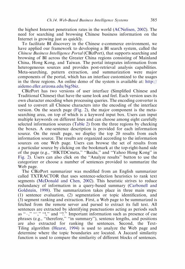
the highest Internet penetration rates in the world (ACNelisen, 2002). Theneed for searching and browsing Chinese business information on theInternet is growing just as quickly.To facilitate BI discovery in the Chinese e-commerce environment, we
have applied our framework to developing a BI search system, called theChinese Business Intelligence Portal (CBizPort), that supports searching andbrowsing of BI across the Greater China regions consisting of MainlandChina, Hong Kong, and Taiwan. The portal integrates information fromheterogeneous sources and provides post-retrieval analysis capabilities.Meta-searching, pattern extraction, and summarization were majorcomponents of the portal, which has an interface customized to the usagesin the three regions. An online demo of the system is available at: http://aidemo.eller.arizona.edu/big5biz.CBizPort has two versions of user interface (Simplified Chinese and
Traditional Chinese) that have the same look and feel. Each version uses itsown character encoding when processing queries. The encoding converter isused to convert all Chinese characters into the encoding of the interfaceversion. On the search page (Fig. 2), the major component is the meta-searching area, on top of which is a keyword input box. Users can inputmultiple keywords on different lines and can choose among eight carefullyselected information sources (Table 2) from the three regions by checkingthe boxes. A one-sentence description is provided for each informationsource. On the result page, we display the top 20 results from eachinformation source. The results are organized according to the informationsources on one Web page. Users can browse the set of results froma particular source by clicking on the bookmark at the top-right-hand sideof the page (e.g., ‘‘HKTDCmeta,’’ ‘‘Baidu,’’ and ‘‘Yahoo Hong Kong’’ inFig. 2). Users can also click on the ‘‘Analyze results’’ button to use thecategorizer or choose a number of sentences provided to summarize theWeb page.The CBizPort summarizer was modified from an English summarizer
called TXTRACTOR that uses sentence-selection heuristics to rank textsegments (McDonald and Chen, 2002). This heuristic strives to reduceredundancy of information in a query-based summary (Carbonell andGoldstein, 1998). The summarization takes place in three main steps:(1) sentence evaluation, (2) segmentation or topic identification, and(3) segment ranking and extraction. First, a Web page to be summarized isfetched from the remote server and parsed to extract its full text. Allsentences are extracted by identifying punctuations acting as periods suchas ‘‘ � ,’’ ‘‘1,’’ ‘‘!,’’ and ‘‘?.’’ Important information such as presence of cuephrases (e.g., ‘‘therefore,’’ ‘‘in summary’’), sentence lengths, and positionsare also extracted for ranking the sentences. Second, the Text-Tiling algorithm (Hearst, 1994) is used to analyze the Web page anddetermine where the topic boundaries are located. A Jaccard similarityfunction is used to compare the similarity of different blocks of sentences.
Ch.14. Web-Based Business Intelligence Systems 385
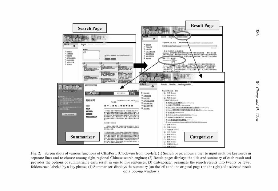
Fig. 2. Screen shots of various functions of CBizPort. (Clockwise from top-left: (1) Search page: allows a user to input multiple keywords in
separate lines and to choose among eight regional Chinese search engines; (2) Result page: displays the title and summary of each result and
provides the options of summarizing each result in one to five sentences; (3) Categorizer: organizes the search results into twenty or fewer
folders each labeled by a key phrase; (4) Summarizer: displays the summary (on the left) and the original page (on the right) of a selected result
on a pop-up window.)
W.ChungandH.Chen
386
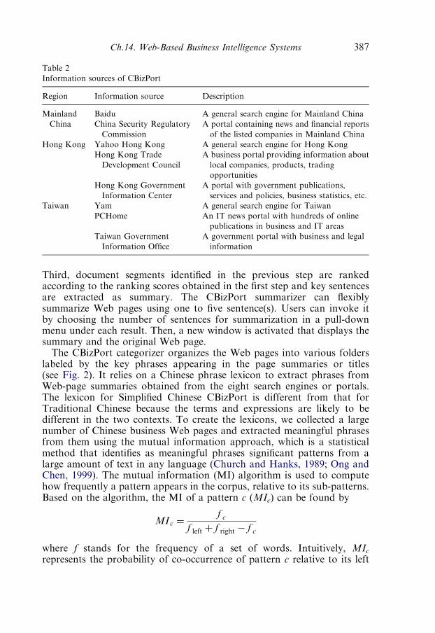
Third, document segments identified in the previous step are rankedaccording to the ranking scores obtained in the first step and key sentencesare extracted as summary. The CBizPort summarizer can flexiblysummarize Web pages using one to five sentence(s). Users can invoke itby choosing the number of sentences for summarization in a pull-downmenu under each result. Then, a new window is activated that displays thesummary and the original Web page.The CBizPort categorizer organizes the Web pages into various folders
labeled by the key phrases appearing in the page summaries or titles(see Fig. 2). It relies on a Chinese phrase lexicon to extract phrases fromWeb-page summaries obtained from the eight search engines or portals.The lexicon for Simplified Chinese CBizPort is different from that forTraditional Chinese because the terms and expressions are likely to bedifferent in the two contexts. To create the lexicons, we collected a largenumber of Chinese business Web pages and extracted meaningful phrasesfrom them using the mutual information approach, which is a statisticalmethod that identifies as meaningful phrases significant patterns from alarge amount of text in any language (Church and Hanks, 1989; Ong andChen, 1999). The mutual information (MI) algorithm is used to computehow frequently a pattern appears in the corpus, relative to its sub-patterns.Based on the algorithm, the MI of a pattern c (MIc) can be found by
MIc ¼f c
f left þ f right � f c
where f stands for the frequency of a set of words. Intuitively, MIcrepresents the probability of co-occurrence of pattern c relative to its left
Table 2
Information sources of CBizPort
Region Information source Description
Mainland
China
Baidu A general search engine for Mainland China
China Security Regulatory
Commission
A portal containing news and financial reports
of the listed companies in Mainland China
Hong Kong Yahoo Hong Kong A general search engine for Hong Kong
Hong Kong Trade
Development Council
A business portal providing information about
local companies, products, trading
opportunities
Hong Kong Government
Information Center
A portal with government publications,
services and policies, business statistics, etc.
Taiwan Yam A general search engine for Taiwan
PCHome An IT news portal with hundreds of online
publications in business and IT areas
Taiwan Government
Information Office
A government portal with business and legal
information
Ch.14. Web-Based Business Intelligence Systems 387
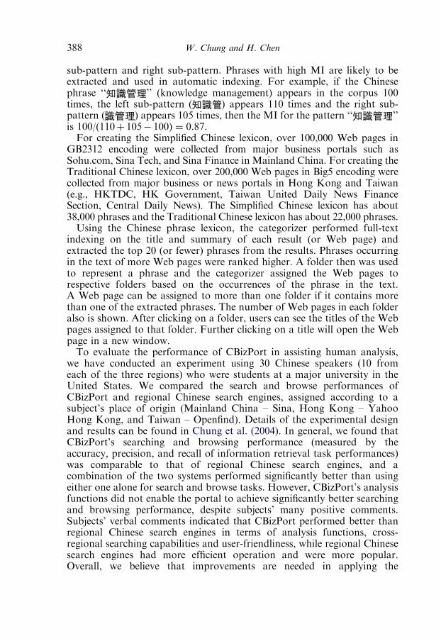
sub-pattern and right sub-pattern. Phrases with high MI are likely to beextracted and used in automatic indexing. For example, if the Chinesephrase ‘‘ ’’ (knowledge management) appears in the corpus 100times, the left sub-pattern ( ) appears 110 times and the right sub-pattern ( ) appears 105 times, then the MI for the pattern ‘‘ ’’is 100/(110þ 105� 100) ¼ 0.87.For creating the Simplified Chinese lexicon, over 100,000 Web pages in
GB2312 encoding were collected from major business portals such asSohu.com, Sina Tech, and Sina Finance in Mainland China. For creating theTraditional Chinese lexicon, over 200,000 Web pages in Big5 encoding werecollected from major business or news portals in Hong Kong and Taiwan(e.g., HKTDC, HK Government, Taiwan United Daily News FinanceSection, Central Daily News). The Simplified Chinese lexicon has about38,000 phrases and the Traditional Chinese lexicon has about 22,000 phrases.Using the Chinese phrase lexicon, the categorizer performed full-text
indexing on the title and summary of each result (or Web page) andextracted the top 20 (or fewer) phrases from the results. Phrases occurringin the text of more Web pages were ranked higher. A folder then was usedto represent a phrase and the categorizer assigned the Web pages torespective folders based on the occurrences of the phrase in the text.A Web page can be assigned to more than one folder if it contains morethan one of the extracted phrases. The number of Web pages in each folderalso is shown. After clicking on a folder, users can see the titles of the Webpages assigned to that folder. Further clicking on a title will open the Webpage in a new window.To evaluate the performance of CBizPort in assisting human analysis,
we have conducted an experiment using 30 Chinese speakers (10 fromeach of the three regions) who were students at a major university in theUnited States. We compared the search and browse performances ofCBizPort and regional Chinese search engines, assigned according to asubject’s place of origin (Mainland China – Sina, Hong Kong – YahooHong Kong, and Taiwan – Openfind). Details of the experimental designand results can be found in Chung et al. (2004). In general, we found thatCBizPort’s searching and browsing performance (measured by theaccuracy, precision, and recall of information retrieval task performances)was comparable to that of regional Chinese search engines, and acombination of the two systems performed significantly better than usingeither one alone for search and browse tasks. However, CBizPort’s analysisfunctions did not enable the portal to achieve significantly better searchingand browsing performance, despite subjects’ many positive comments.Subjects’ verbal comments indicated that CBizPort performed better thanregional Chinese search engines in terms of analysis functions, cross-regional searching capabilities and user-friendliness, while regional Chinesesearch engines had more efficient operation and were more popular.Overall, we believe that improvements are needed in applying the
W. Chung and H. Chen388

framework to addressing the heterogeneity and unmonitored quality ofinformation on the Web.
4.2 Case 2: Exploring BI using Web visualization techniques
As reported by Fuld et al. (2003), existing BI tools suffer from a lack ofanalysis and visualization capabilities because many of them do not revealunderlying structure of the data. This case study examines the use of clusteringand visualization techniques to assist analysts in exploring BI on the Web. Wehave applied our framework to developing a system, called BusinessIntelligence Explorer (BIE), that assists in the discovery and exploration ofBI from a large number of Web pages. Data in the form of Web pages werecollected by meta-searching seven major search engines (AltaVista, Allthe-Web, Yahoo, MSN, LookSmart, Teoma, and Wisenut) using nine BI queriesobtained by searching the INSPEC literature database. In total we collected3,149 Web pages from 2,860 business Web sites. Each Web page representedone Web site. Then we performed automatic parsing and indexing to extractkey terms from the pages, which were used as inputs of co-occurrenceanalysis, transforming raw data (indexes and weights) into a matrix showingthe similarity between every pair of Web sites. The similarity betweenevery pair of Web sites contained its content, structural (connectivity),and cocitation information, as shown in Fig. 3 (Chen and Lynch, 1992).
Similarity between site i and site j =
222
1C
C
S
S
A
AW ijijij
ij
where A, S, C are matrices for Aij, Sij, Cij respectively. 0 < , < 1, and 0 + 1Aij = 1 if site i has a hyperlink to site j, Aij = 0 otherwiseSij = Asymmetric similarity score between site i and site j
n
ki
p
kkjki
jiij
d
ddDDsimS
2
1
k 1
m
ki
p
kkjki
d
dd
2
1
k 1
, ijji DDsimS ,
where n = total number of terms in Di
m = total number of terms in Dj
p = total number of terms that appear in both Di and Dj
jjj
ijij factortypeTermwdf
Ntfd log
tfij = number of occurrence of term j in Web page idfj = number of Web pages containing term jwj = number of words in term j
textalternateimageinappearsjtermif
textcontentinappearsjtermif
headinginappearsjtermif
titleinappearsjtermif
typewheretype
factortypeTerm jj
j
4
,3
,2
,1
min10
2101
Cij = number of Web sites pointing to both site i and site j (co-citation matrix)
Fig. 3. Formulae used in co-occurrence analysis.
Ch.14. Web-Based Business Intelligence Systems 389
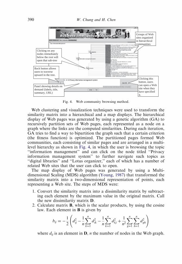
Web clustering and visualization techniques were used to transform thesimilarity matrix into a hierarchical and a map displays. The hierarchicaldisplay of Web pages was generated by using a genetic algorithm (GA) torecursively partition sets of Web pages, each represented as a node on agraph where the links are the computed similarities. During each iteration,GA tries to find a way to bipartition the graph such that a certain criterion(the fitness function) is optimized. The partitioned pages formed Webcommunities, each consisting of similar pages and are arranged in a multi-level hierarchy as shown in Fig. 4, in which the user is browsing the topic‘‘information management’’ and can click on the node titled ‘‘Privacyinformation management system’’ to further navigate such topics as‘‘digital libraries’’ and ‘‘Lotus organizer,’’ each of which has a number ofrelated Web sites that the user can click to open.The map display of Web pages was generated by using a Multi-
dimensional Scaling (MDS) algorithm (Young, 1987) that transformed thesimilarity matrix into a two-dimensional representation of points, eachrepresenting a Web site. The steps of MDS were:
1. Convert the similarity matrix into a dissimilarity matrix by subtract-ing each element by the maximum value in the original matrix. Callthe new dissimilarity matrix D.
2. Calculate matrix B, which is the scalar products, by using the cosinelaw. Each element in B is given by
bij ¼ �1
2d2ij �
1
n
Xnk¼1
d2ik �
1
n
Xnk¼1
d2kj þ
1
n2
Xng¼1
Xnh¼1
d2gh
!
where dij is an element in D, n the number of nodes in the Web graph.
Groups of Web sites organized in hierarchical communities
Panel showing details on demand (labels, title, summary, URL)
Back button allows users to traverse upward in the tree.
Clicking on any nodes immediately below the root will open that sub-tree
Clicking this button, users can open a Web site when they have specified it.
Fig. 4. Web community browsing method.
W. Chung and H. Chen390
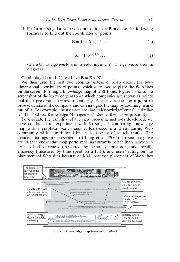
3. Perform a singular value decomposition on B and use the followingformulae to find out the coordinates of points.
B ¼ U� V�U0 . . . (1)
X ¼ U� V1=2 . . . (2)
where U has eigenvectors in its columns and V has eigenvectors on itsdiagonal.
Combining (1) and (2), we have B ¼ X�Xu.We then used the first two column vectors of X to obtain the two-
dimensional coordinates of points, which were used to place the Web siteson the screen, forming a knowledge map of a BI topic. Figure 5 shows thescreenshot of the knowledge map on which companies are shown as pointsand their proximities represent similarity. A user can click on a point tobrowse details of the company and can navigate the map by zooming in andout of it. For example, the user can see that ‘‘eKnowledgeCenter’’ is similarto ‘‘IT Toolbox Knowledge Management’’ due to their close proximity.To evaluate the usability of the new browsing methods developed, we
have conducted an experiment with 30 subjects comparing knowledgemap with a graphical search engine, Kartoo.com, and comparing Webcommunity with a traditional linear list display of search results. Thedetailed findings are presented in Chung et al. (2005). In summary, wefound that knowledge map performed significantly better than Kartoo interms of effectiveness (measured by accuracy, precision, and recall),efficiency (measured by time spent on a task), and users’ rating on theplacement of Web sites because of KMs accurate placement of Web sites
Panel showing details (title, URL summary)
The closeness ofany two points reflects their similarity
Navigation buttons allow browsing in four directionsDetails of this Web
site is being shown on the bottom panel Users can control the
number of Web sites to be displayed
Zooming buttons allow zoom-in or zoom-out functions
Fig. 5. Knowledge map browsing method.
Ch.14. Web-Based Business Intelligence Systems 391

and its clean interface. Web community performed significantly better thanresult lists in terms of effectiveness, efficiency, and usability.
4.3 Case 3: Business stakeholder analysis using Web classificationtechniques
Business stakeholder analysis has been complicated by the use of theWeb, which has allowed much greater variety and number of stakeholders(than in the past) to establish relationships to a company via hyperlinkconnections, distributed databases, online forums, intranets and extranets,and other Web-enabled technologies. These multitudes of stakeholdersmay include individuals, international businesses, local and regionalsuppliers, government agencies, and global organizations. As a result,business managers and analysts find it increasingly difficult to understandand to address the needs of stakeholders. Although traditional stakeholderanalysis approaches (e.g., Donaldson and Preston, 1995; Freeman, 1984;Mitchell et al., 1997) offer theoretical foundations for understandingbusiness relationships, they are largely manually driven and not scalable tothe rapid growth and change of the Web. In this case study, we have appliedour framework to business stakeholder analysis on the Web, with a goal ofassisting business analysts in better understanding stakeholder relationshipson the Web.We have collected Web pages of business stakeholders of the top 100
knowledge management companies identified by the Knowledge Manage-ment World (KMWorld.com) Web site (McKellar, 2003), a major Webportal providing news, publications, online resources, and solutions to morethan 51,000 subscribers in the knowledge management systems market.To identify such stakeholders, we used the back-link search function of theGoogle search engine (http://www.google.com/) to search for Web pageshaving hyperlinks pointing to the companies’ Web sites. For each of the 100KM (host) companies, we considered only the first 100 results returnedfrom Google in order to limit the scope of analysis. After filtering self-linksand duplicating results, we obtained 3,713 Web pages, or 37 stakeholdersper host company.A BI expert having a doctorate degree and years of industry and
academic experiences helped us to develop a domain lexicon consisting of329 key terms for distinguishing among 11 business stakeholder types,which were modified from Reid (2003) and are shown in Table 3. These keyterms were selected from the 414 collected Web pages of 9 companiesrandomly chosen from the 100 KM companies for training the algorithmsto be used in automatic classification of business stakeholder pages.Next, the expert manually classified each of the 414 stakeholder pages
of the 9 selected companies into one of the 11 stakeholder types (listed inTable 3). These tagged pages serve as a training set of stakeholders.
W. Chung and H. Chen392
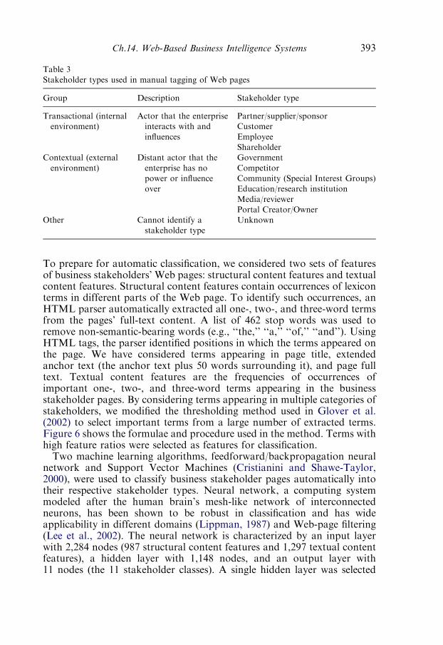
To prepare for automatic classification, we considered two sets of featuresof business stakeholders’ Web pages: structural content features and textualcontent features. Structural content features contain occurrences of lexiconterms in different parts of the Web page. To identify such occurrences, anHTML parser automatically extracted all one-, two-, and three-word termsfrom the pages’ full-text content. A list of 462 stop words was used toremove non-semantic-bearing words (e.g., ‘‘the,’’ ‘‘a,’’ ‘‘of,’’ ‘‘and’’). UsingHTML tags, the parser identified positions in which the terms appeared onthe page. We have considered terms appearing in page title, extendedanchor text (the anchor text plus 50 words surrounding it), and page fulltext. Textual content features are the frequencies of occurrences ofimportant one-, two-, and three-word terms appearing in the businessstakeholder pages. By considering terms appearing in multiple categories ofstakeholders, we modified the thresholding method used in Glover et al.(2002) to select important terms from a large number of extracted terms.Figure 6 shows the formulae and procedure used in the method. Terms withhigh feature ratios were selected as features for classification.Two machine learning algorithms, feedforward/backpropagation neural
network and Support Vector Machines (Cristianini and Shawe-Taylor,2000), were used to classify business stakeholder pages automatically intotheir respective stakeholder types. Neural network, a computing systemmodeled after the human brain’s mesh-like network of interconnectedneurons, has been shown to be robust in classification and has wideapplicability in different domains (Lippman, 1987) and Web-page filtering(Lee et al., 2002). The neural network is characterized by an input layerwith 2,284 nodes (987 structural content features and 1,297 textual contentfeatures), a hidden layer with 1,148 nodes, and an output layer with11 nodes (the 11 stakeholder classes). A single hidden layer was selected
Table 3
Stakeholder types used in manual tagging of Web pages
Group Description Stakeholder type
Transactional (internal
environment)
Actor that the enterprise
interacts with and
influences
Partner/supplier/sponsor
Customer
Employee
Shareholder
Contextual (external
environment)
Distant actor that the
enterprise has no
power or influence
over
Government
Competitor
Community (Special Interest Groups)
Education/research institution
Media/reviewer
Portal Creator/Owner
Other Cannot identify a
stakeholder type
Unknown
Ch.14. Web-Based Business Intelligence Systems 393
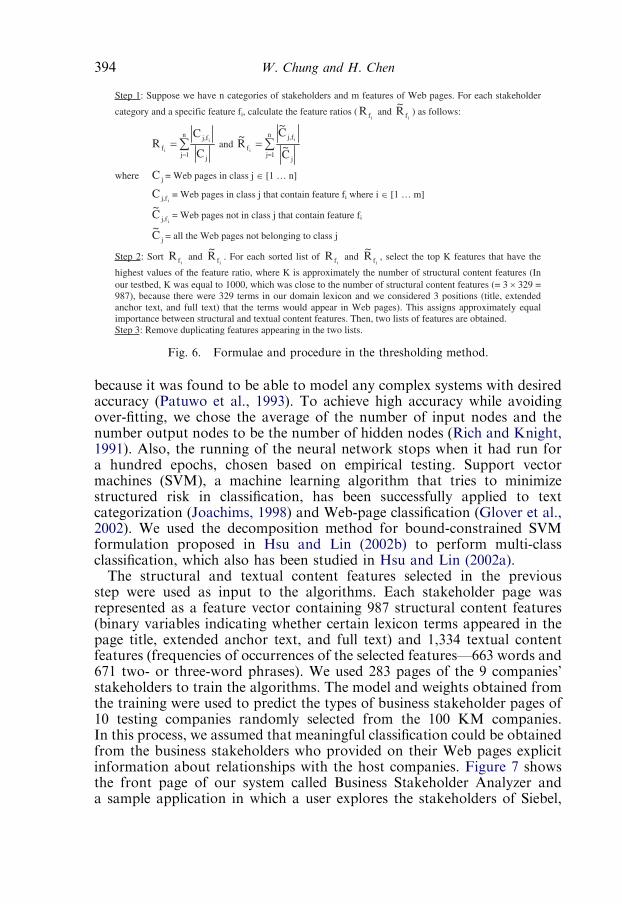
because it was found to be able to model any complex systems with desiredaccuracy (Patuwo et al., 1993). To achieve high accuracy while avoidingover-fitting, we chose the average of the number of input nodes and thenumber output nodes to be the number of hidden nodes (Rich and Knight,1991). Also, the running of the neural network stops when it had run fora hundred epochs, chosen based on empirical testing. Support vectormachines (SVM), a machine learning algorithm that tries to minimizestructured risk in classification, has been successfully applied to textcategorization (Joachims, 1998) and Web-page classification (Glover et al.,2002). We used the decomposition method for bound-constrained SVMformulation proposed in Hsu and Lin (2002b) to perform multi-classclassification, which also has been studied in Hsu and Lin (2002a).The structural and textual content features selected in the previous
step were used as input to the algorithms. Each stakeholder page wasrepresented as a feature vector containing 987 structural content features(binary variables indicating whether certain lexicon terms appeared in thepage title, extended anchor text, and full text) and 1,334 textual contentfeatures (frequencies of occurrences of the selected features—663 words and671 two- or three-word phrases). We used 283 pages of the 9 companies’stakeholders to train the algorithms. The model and weights obtained fromthe training were used to predict the types of business stakeholder pages of10 testing companies randomly selected from the 100 KM companies.In this process, we assumed that meaningful classification could be obtainedfrom the business stakeholders who provided on their Web pages explicitinformation about relationships with the host companies. Figure 7 showsthe front page of our system called Business Stakeholder Analyzer anda sample application in which a user explores the stakeholders of Siebel,
Fig. 6. Formulae and procedure in the thresholding method.
W. Chung and H. Chen394

a. Front page of Business Stakeholder Analyzer – Subjects could browse through definitionsof stakeholder types, examples of stakeholder pages, and three business stakeholder groups.
b. Business stakeholders of Siebel.
Fig. 7. Business Stakeholder Analyzer.
Ch.14. Web-Based Business Intelligence Systems 395
a major company specializing on customer relationship management. Thestakeholders were identified and classified automatically by the aforemen-tioned techniques.We have conducted an experiment with 36 student subjects to evaluate
the performance of applying the framework to stakeholder classifica-tion compared with human users and with random classification (thebaseline). Detailed experimental results are presented in Chung et al.(forthcoming). In summary, we found that the use of any combination offeatures and techniques in automatic stakeholder classification outper-formed the baseline method significantly (measured by classificationaccuracy). Overall, humans were more effective than NN or SVM, butthe algorithms outperformed human judgment in classifying certainstakeholder types such as partners/sponsors/suppliers and community.Subjects perceived the automatic classification very favorably as helpingbusiness analysts identify and classify business stakeholders.
5 Summary and future directions
In this chapter, we have reviewed related work on BI systems and miningthe Web for BI, described a framework for discovering BI on the Web, andpresented three case studies applying the framework to discovering BI onthe Web. The framework was found to help to meet analysis needs thatwould otherwise require substantial human effort. Such needs includesummarizing, classifying, visualizing, exploring the information landscape,and extracting relationships. Each case study demonstrates how certainanalysis needs in discovering BI can be fulfilled, thereby freeing humans toperform other value-added work. Considering the scarce research workfound (Negash, 2004), this chapter presents new advances in the BI fieldand provides practical insights to BI practitioners and system developers.Several directions are worth exploring for researchers and practitioners.
Developing Web-based systems to support discovery of BI in otherlanguages than English (or Chinese described in Section 4.1) will bepromising considering the multinational nature of the Web in supportingbusiness operations. For example, Spanish and Arabic are two majorlanguages used in South America and the Middle East, respectively. Ascommercial activities of these regions are growing significantly in recentyears, systems that support effective and efficient discovery of BI on theWeb will assist managers and analysts in understanding their businessenvironment. However, new visualization metaphors for BI exploration willfurther assist effective and efficient discovery of BI on the Web. Metaphorsthat exploit the nature of the Web as well as features of a specific domainmay bring a more satisfactory and pleasurable browsing experienceto users. Type-specific stakeholder analysis can be performed to further
W. Chung and H. Chen396

support Web-based stakeholder analysis. Multinational business partner-ships and cooperation also can be analyzed through explicit informationposted on the Web.
References
ACNelisen (2002). Nelisen//Netratings reports a record half billion people worldwide now have home
Internet access [Online]. Available at http://asiapacific.acnielsen.com.au/news.asp?newsID ¼ 74
Adomavicius, G., A. Tuzhilin (2001). Using data mining methods to build customer profiles. IEEE
Computer 34(2), 74–82.
Bowman, C.M., P.B. Danzig, U. Manber, F. Schwartz (1994). Scalable Internet resource discovery:
research problems and approaches. Communications of the ACM 37(8), 98–107.
Brin, S., L. Page (1998). The anatomy of a large-scale hypertextual Web search engine, in: Proceedings of
the 7th International WWW Conference, Brisbane, Australia.
Broder, A., R. Kumar, F. Maghoul, P. Raghavan, S. Rajagopolan, R. Stata, A. Tomkins, J.L. Wiener
(2000). Graph structure in the Web, in: Proceedings of the 9th International World Wide Web
Conference, Elsevier Science, Amsterdam, The Netherlands, pp. 309–320.
Carbonell, J., J. Goldstein (1998). The use of MMR: diversity-based reranking for reordering
documents and producing summaries, in: Proceedings of the 21st Annual International ACM-SIGIR
Conference on Research and Development in Information Retrieval, Melbourne, ACM Press,
Australia, pp. 335–336.
Carvalho, R., M. Ferreira (2001). Using information technology to support knowledge conversion
processes. Information Research 7(1).
Chakrabarti, S., B. Dom, R.S. Kumar, P. Raghavan, S. Rajagopalan, A. Tomkins, D. Gibson,
J. Kleinberg (1999). Mining the web’s link structure. IEEE Computer 32(8), 60–67.
Chen, H., M. Chau (2004). Web mining: machine learning for web applications, in: M.E. Williams (ed.),
Annual Review of Information Science and Technology (ARIST). Information Today, Inc, Medford,
NJ, pp. 289–329.
Chen, H., H. Fan, M. Chau, D. Zeng (2001). MetaSpider: meta-searching and categorization on the
web. Journal of the American Society for Information Science and Technology 52(13), 1134–1147.
Chen, H., A. Houston, R. Sewell, B. Schatz (1998). Internet browsing and searching: user evaluation of
category map and concept space techniques. Journal of the American Society for Information Science,
Special Issue on AI Techniques for Emerging Information Systems Applications 49(7), 582–603.
Chen, H., K.J. Lynch (1992). Automatic construction of networks of concepts characterizing document
databases. IEEE Transactions on Systems, Man, and Cybernetics 22(5), 885–902.
Chen, H., C. Schuffels, R. Orwig (1996). Internet categorization and search: a self-organizing approach.
Journal of Visual Communication and Image Representation 7(1), 88–102.
Chen, H.M., M.D. Cooper (2001). Using clustering techniques to detect usage patterns in a Web-based
information system. Journal of the American Society for Information and Science and Technology
52(11), 888–904.
Choo, C.W. (1998). The Knowing Organization. Oxford University Press, Oxford.
Chung, W., H. Chen, E. Reid (forthcoming). Business stakeholder analyzer: An experiment of
classifying stakeholders on the web. Journal of the American Society for Information Science and
Technology (fully accepted, published online, print version forthcoming).
Chung, W., H. Chen, J.F. Nunamaker (2005). A visual framework for knowledge discovery on the Web:
an empirical study on business intelligence exploration. Journal of Management Information Systems
21(4), 57–84.
Chung, W., Y. Zhang, Z. Huang, G. Wang, T.-H. Ong, H. Chen (2004). Internet searching and
browsing in a multilingual world: an experiment on the Chinese business intelligence portal
(CBizPort). Journal of the American Society for Information Science and Technology 55(9), 818–831.
Ch.14. Web-Based Business Intelligence Systems 397

Church, K., P. Hanks (1989). Word association norms, mutual information, and lexicography, in:
Proceedings of the 27th Annual Meeting of Association for Computational Linguistics, Vancouver, BC,
Canada, pp. 76–83.
CNNIC (2002). Analysis report on the growth of the Internet in China, China Internet Network
Information Center [Online]. Available at http://www.cnnic.net.cn/develst/2002-7e/6.shtml
Cristianini, N., J. Shawe-Taylor (2000). An Introduction to Support Vector Machines and Other Kernel-
based Learning Methods. Cambridge University Press, Cambridge, UK.
Cronin, B. (2000). Strategic intelligence and networked business. Journal of Information Science 26,
133–138.
Donaldson, T., L.E. Preston (1995). The stakeholder theory of the corporation: concepts, evidence and
implications. Academy of Management Review 20(1), 65–91.
Etzioni, O. (1996). The world-wide web: quagmire or gold mine? Communications of the ACM 39(11),
65–68.
Freeman, E. (1984). Strategic Management: A Stakeholder Approach. Pitman, Marshfield, MA.
Fuld, L.M., K. Sawka, J. Carmichael, J. Kim, K. Hynes (2002). Intelligence Software ReportTM 2002.
Fuld & Company Inc, Cambridge, MA.
Fuld, L.M., A. Singh, K. Rothwell, J. Kim (2003). Intelligence Software ReportTM 2003: Leveraging the
Web. Fuld & Company Inc, Cambridge, MA.
Futures-Group (1998). Ostriches & Eagles 1997, in: The Futures Group Articles, Glastonbury, CT.
Global Reach (2004a). Evolution of non-English online populations [Online]. Available at http://
global-reach.biz/globstats/evol.html
Global Reach (2004b). Global Internet Statistics (by Language) [Online]. Available at http://
www.glreach.com/globstats/
Glover, E.J., K. Tsioutsiouliklis, S. Lawrence, D.M. Pennock, G.W. Flake (2002). Using Web structure
for classifying and describing Web pages, in: Proceedings of the 11th International World Wide Web
Conference, Honolulu, Hawaii.
Hearst, M.A. (1994). Multi-paragraph segmentation of expository text, in: Proceedings of the 32th
Annual Meeting of the Association for Computational Linguistics, Las Cruces, NM, pp. 9–16.
Hearst, M.A. (1999). Untangling text data mining, in: Proceedings of the 37th Annual Meeting of the
Association for Computational Linguistics, The Association for Computational Linguistics, College
Park, MD.
Henzinger, M.R., S. Lawrence (2004). Extracting knowledge from the world wide web. in: Proceedings
of the National Academy of Sciences of the United States of America.
Hsu, C.W., C.J. Lin (2002a). A comparison on methods for multi-class support vector machines.
IEEE Transactions on Neural Networks 13(2), 415–425.
Hsu, C.W., C.J. Lin (2002b). A simple decomposition method for support vector machines. Machine
Learning 46(1–3), 291–314.
Hurst, M. (2001). Layout and language: challenges for table understanding on the Web, in: Proceedings
of the 1st International Workshop on Web Document Analysis, Seattle, WA, pp. 27–30.
Jain, A.K., R.C. Dubes (1988). Algorithms for Clustering Data. Prentice-Hall, Englewood Cliffs, NJ.
Joachims, T. (1998). Text categorization with support vector machines: Learning with many relevant
features, in: Proceedings of the Tenth European Conference on Machine Learning, Springer Verlag,
Chemnitz, Germany, pp. 137–142.
Kleinberg, J. (1999). Authoritative sources in a hyperlinked environment. Journal of the Association of
Computing Machinery 46(5), 604–632.
Kosala, R., H. Blockeel (2000). Web mining research: a survey. ACM SIGKDD Explorations 2(1), 1–15.
Kwon, O.-W., J.-H. Lee (2003). Text categorization based on k-nearest neighbor approach for web site
classification. Information Processing & Management 39(1), 25–44.
Lee, P.Y., S.C. Hui, A. Cheuk, M. Fong (2002). Neural networks for web content filtering. IEEE
Intelligent Systems 17(5), 48–57.
Lempel, R., S. Moran (2001). SALSA: the stochastic approach for link-structure analysis. ACM
Transactions on Information Systems 19(2), 131–160.
W. Chung and H. Chen398
Lippman, R.P. (1987). Introduction to computing with neural networks. IEEE ASSPMagazine 4(2), 4–22.
Lyman, P., H. Varian (2003). How much information? University of California, Berkeley [Online].
Available at http://www.sims.berkeley.edu:8000/research/projects/how-much-info-2003/.
McDonald, D., H. Chen (2002). Using sentence selection heuristics to rank text segments in
TXTRACTOR, in: Proceedings of the second ACM/IEEE-CS Joint Conference on Digital Libraries,
ACM/IEEE-CS, Portland, OR, pp. 28–35.
McKellar, H. (2003). KMWorld’s 100 Companies that Matter in Knowledge Management 2003, KM
World [Online]. Available at http://www.kmworld.com/100.cfm
Menczer, F. (2004). Evolution of document networks. in: Proceedings of the National Academy of
Sciences of the United States of America.
Mendelzon, A.O., D. Rafiei (2000). What do the neighbours think? Computing web page reputations.
IEEE Data Engineering Bulletin 23(3), 9–16.
Mitchell, R.K., B.R. Agle, D.J. Wood (1997). Toward a theory of stakeholder identification and
salience: defining the principle of who and what really counts. Academy of Management Review 22(4),
853–886.
Mladenic, D. (1998). Turning Yahoo into an Automatic Web Page Classifier, in: Proceedings of the 13
European Conference on Artificial Intelligence, Brighton, UK, pp. 473–474.
Nasukawa, T., T. Nagano (2001). Text analysis and knowledge mining system. IBM Systems Journal
40(4), 967–984.
Negash, S. (2004). Business intelligence. Communications of the Association for Information Systems 13,
177–195.
Nolan, J. (1999). Confidential: Uncover Your Competitor’s Secrets Legally and Quickly and Protect Your
Own. Harper Business, New York.
Ong, T.-H., H. Chen (1999). Updateable PAT-array approach for Chinese key phrase extraction using
mutual information: a linguistic foundation for knowledge management, in: Proceedings of the
Second Asian Digital Library Conference, Taipei, Taiwan, pp. 63–84.
Patuwo, E., M.S. Hu, M.S. Hung (1993). Two-group classification using neural networks. Decision
Sciences 24(4), 825–845.
Pazzani, M. (1999). A framework for collaborative, content-based and demographic filtering. Artificial
Intelligence Review 13(5), 393–408.
Reid, E.O.F. (2003). Identifying a company’s non-customer online communities: a Proto-typology, in:
Proceedings of the 36th Hawaii International Conference on System Sciences (HICSS-36), IEEE
Computer Society, Island of Hawaii, HI.
Rich, E., K. Knight (1991). Learning in Neural Networks, in: Artificial Intelligence (2nd ed.), McGraw-
Hill, Inc., New York, pp. 500–507.
Roussinov, D., H. Chen (2001). Information navigation on the Web by clustering and summarizing
query results. Information Processing and Management 37(6), 789–816.
Schatz, B. (2002). The Interspace: concept navigation across distributed communities. IEEE Computer
35(1), 54–62.
Shneiderman, B. (1996). The eyes have it: a task by data type taxonomy for information visualizations,
in: Proceedings of Visual Languages, IEEE Computer Society, Boulder, CO, pp. 336–343.
Soper, D.S. (2005). A framework for automated Web business intelligence systems, in: Proceedings of
the 38th Hawaii International Conference on System Sciences, IEEE Computer Society, Island of
Hawaii, HI.
Spence, R. (2001). Information Visualization. ACM Press, New York, NY.
Taylor, R.S. (1986). Value-added Processes in Information Systems. Ablex, Norwood, NJ.
Trybula, W.J. (1999). Text mining, in: M.E. Williams (ed.), Annual Review of Information Science and
Technology. Information Today, Inc, Medford, NJ, pp. 385–419.
van Rijsbergen, C.J. (1979). Information Retrieval. 2nd ed. Butterworths, London.
Westney, E., S. Ghoshal (1994). Building a competitor intelligence organization: adding value in an
information function, in: T.J. Allen, M.S. Scott (eds.), Information Technology and the Corporation in
the 1990s: Research Studies. Oxford University Press, New York, pp. 430–453.
Ch.14. Web-Based Business Intelligence Systems 399

Yang, C.C., H. Chen, K. Hong (2003). Visualization of large category map for Internet browsing.
Decision Support Systems 35(1), 89–102.
Young, F.W. (1987). Multidimensional Scaling: History, Theory, and Applications. Lawrence Erlbaum
Associates, Hillsdale, NJ.
Zamir, O., O. Etzioni (1999). Grouper: a dynamic clustering interface to Web search results, in:
Proceedings of the 8th World Wide Web Conference, Toronto, Canada.
Zhong, N., J. Liu, Y. Yao (eds.) (2003). Web Intelligence. Springer, New York, NY.
W. Chung and H. Chen400