BUS 525: Managerial Economics

Lecture 5

The Production Process and Costs

OverviewI. Production Analysis

– Total Product, Marginal Product, Average Product– Isoquants– Isocosts– Cost Minimization

II. Cost Analysis– Total Cost, Variable Cost, Fixed Costs– Cubic Cost Function– Cost Relations

III. Multi-Product Cost Functions

Production Analysis

• Production Function– A function that defines the maximum amount

output that can be produced with a given set of inputs

• Q = F(K,L)• The maximum amount of output that can be

produced with K units of capital and L units of labor.

• Short-Run vs. Long-Run Decisions• Fixed vs. Variable Factors of Production

Refer to Table 5.1 Page 1581-4

Total Product

• The maximum level of output that can be produced with a given amount of input

• Cobb-Douglas Production Function• Example: Q = F(K,L) = K.5 L.5

– K is fixed at 16 units. – Short run production function:

Q = (16).5 L.5 = 4 L.5

– Production when 100 units of labor are used?

Q = 4 (100).5 = 4(10) = 40 units

Average Productivity Measures

• Average Product of Labor: A measure of the output produced per unit of input

• APL = Q/L.• Measures the output of an “average” worker.• Average Product of Capital• APK = Q/K.• Measures the output of an “average” unit of

capital.

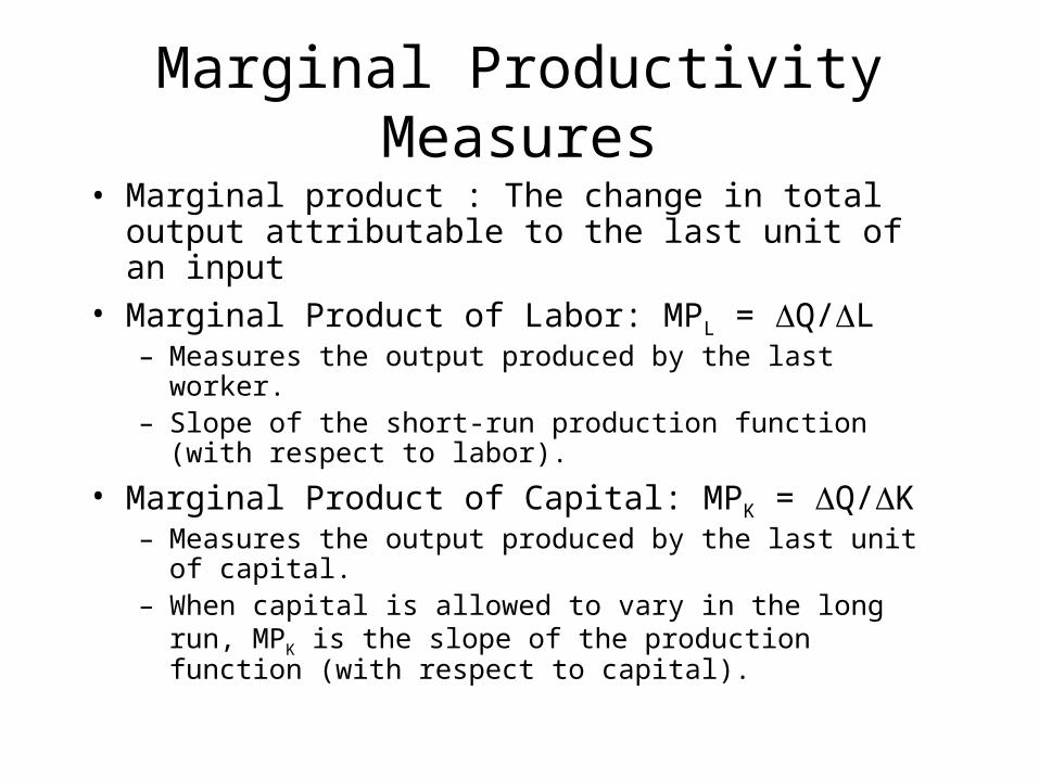
Marginal Productivity Measures

• Marginal product : The change in total output attributable to the last unit of an input

• Marginal Product of Labor: MPL = Q/L– Measures the output produced by the last worker.– Slope of the short-run production function (with respect to

labor).

• Marginal Product of Capital: MPK = Q/K– Measures the output produced by the last unit of capital.– When capital is allowed to vary in the long run, MPK is the

slope of the production function (with respect to capital).

Class Exercise

Given the Cobb-Douglas Production Function

Q = F(K,L) = K.5 L.5, K = 16, L=64Find out the

(i) Average Product of Labor (APl),

(ii) Average Product of Capital (APk),

(iii) Marginal Product of Capital (MPl)

(iv) Marginal Product of Capital (MPk)

Q

L

Q=F(K,L)

IncreasingMarginalReturns

DiminishingMarginalReturns

NegativeMarginalReturns

MP

AP

Increasing, Diminishing and Negative Marginal Returns

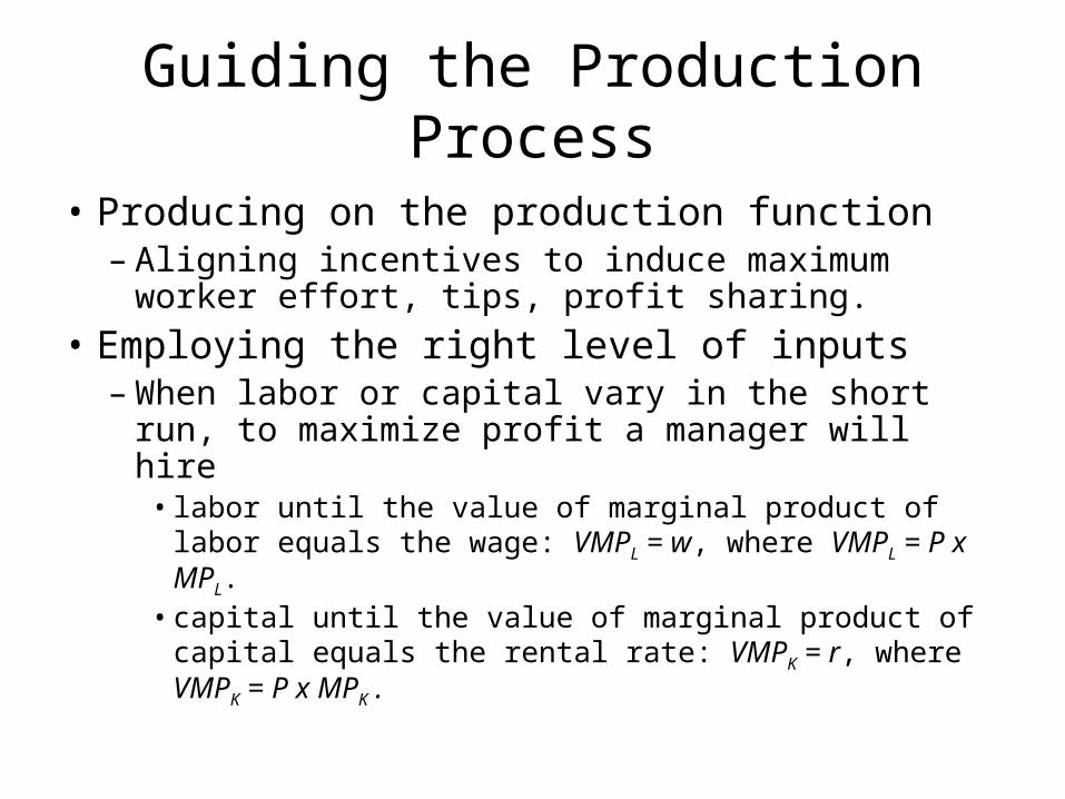
Guiding the Production Process

• Producing on the production function– Aligning incentives to induce maximum worker

effort, tips, profit sharing.

• Employing the right level of inputs– When labor or capital vary in the short run, to

maximize profit a manager will hire• labor until the value of marginal product of labor

equals the wage: VMPL = w, where VMPL = P x MPL.• capital until the value of marginal product of capital

equals the rental rate: VMPK = r, where VMPK = P x MPK .

The profit maximizing usage of inputs

∏ = R- C,

Q = F (K,L), C = wL + rK

∏ = P. F(K,L) - wL - rK

price its equalsproduct margimal of valueits where

point the toup used bemust input each i.e

wV andr V

wP. andr P.L

L)F(K, and

K

L)F(K, Since

0wL

L)F(K,P.

L

π

0rK

L)F(K,P.

K

π

MPMPMPMP

MPMP

LK

LK

Lk

Refer to Table 5.2 Page 163

Isoquant

• The combinations of inputs (K, L) that yield the producer the same level of output.

• The shape of an isoquant reflects the ease with which a producer can substitute among inputs while maintaining the same level of output.

Slope of Isoquant

L

K

MP

MP

KL)/F(K,

LL)/F(K,

dL

dK or,

0] dQ

isoquant an along changenot dooutput Since[

0.L

L)F(K,.

K

L)F(K, dQ

L)(K, F Q

isoquants of Slope

dLdK

Marginal Rate of Technical Substitution (MRTS)

• The rate at which two inputs are substituted while maintaining the same output level.

• The production function satisfies the law of diminishing marginal rate of technical substitution: As a producer uses less of an input, increasingly more of the other input must be employed to produce the same level of output

K

LKL MP

MPMRTS

Linear Isoquants

• Capital and labor are perfect substitutes

• Q = aK + bL

• MRTSKL = b/a

• Linear isoquants imply that inputs are substituted at a constant rate, independent of the input levels employed.

Q3Q2Q1

Increasing Output

L

K

Leontief Isoquants

• Capital and labor are perfect complements.

• Capital and labor are used in fixed-proportions.

• Q = min {bK, cL}

• What is the MRTSKL?

Q3

Q2

Q1

K

Increasing Output

L

Cobb-Douglas Isoquants

• Inputs are not perfectly substitutable.

• Diminishing marginal rate of technical substitution.– As less of one input is used in

the production process, increasingly more of the other input must be employed to produce the same output level.

• Q = KaLb

• MRTSKL = MPL/MPK

Q1

Q2

Q3

K

L

Increasing Output

Isocost• The combinations of inputs

that produce a given level of output at the same cost:

wL + rK = C• Rearranging,

K= (1/r)C - (w/r)L• For given input prices,

isocosts farther from the origin are associated with higher costs.

• Changes in input prices change the slope of the isocost line.

K

LC1

L

KNew Isocost Line for a decrease in the wage (price of labor: w0 > w1).

C1/r

C1/wC0

C0/w

C0/r

C/w0 C/w1

C/r

New Isocost Line associated with higher costs (C0 < C1).

isocost of Slope

r

w - Slope

)(r

1 K

C rK wL

Lr

wC

Cost Minimization

Q

L

K

Point of Cost Minimization

Slope of Isocost =

Slope of Isoquant

A

C

Cost minimization

MRTSMPMP

KLK

L

KF(K,L)/

LF(K,L)/

r

w

by dividing

)(........F(K,L)Qμ

H

)........(K

F(K,L)μr

K

H

)........(L

F(K,L)μw

L

H

][Q- F(K,L) rK wL H

Lagrangian

21

3.......0

20

10

L)F(K, Q subject torK wLMinimize

L)F(K, Q rK, wL C

Cost Minimization

• Marginal product per dollar spent should be equal for all inputs:

• But, this is just

r

w

MP

MP

r

MP

w

MP

K

LKL

r

wMRTSKL

Optimal Input Substitution

• A firm initially produces Q0 by employing the combination of inputs represented by point A at a cost of C0.

• Suppose w0 falls to w1.– The isocost curve rotates

counterclockwise; which represents the same cost level prior to the wage change.

– To produce the same level of output, Q0, the firm will produce on a lower isocost line (C1) at a point B.

– The slope of the new isocost line represents the lower wage relative to the rental rate of capital.

Q0

0

A

L

K

C0/w1C0/w0 C1/w1L0 L1

K0

K1

B

Cost Analysis

• Types of Costs– Fixed costs (FC)– Variable costs (VC)– Total costs (TC)– Sunk costs

• A cost that is forever lost after it has been incurred. Once paid they are irrelevant to decision making

Refer to Table 5.3 Page 179

Total and Variable Costs

C(Q): Minimum total cost of producing alternative levels of output:

C(Q) = VC(Q) + FC

VC(Q): Costs that vary with output.

FC: Costs that do not vary with output.

$

Q

C(Q) = VC + FC

VC(Q)

FC

0

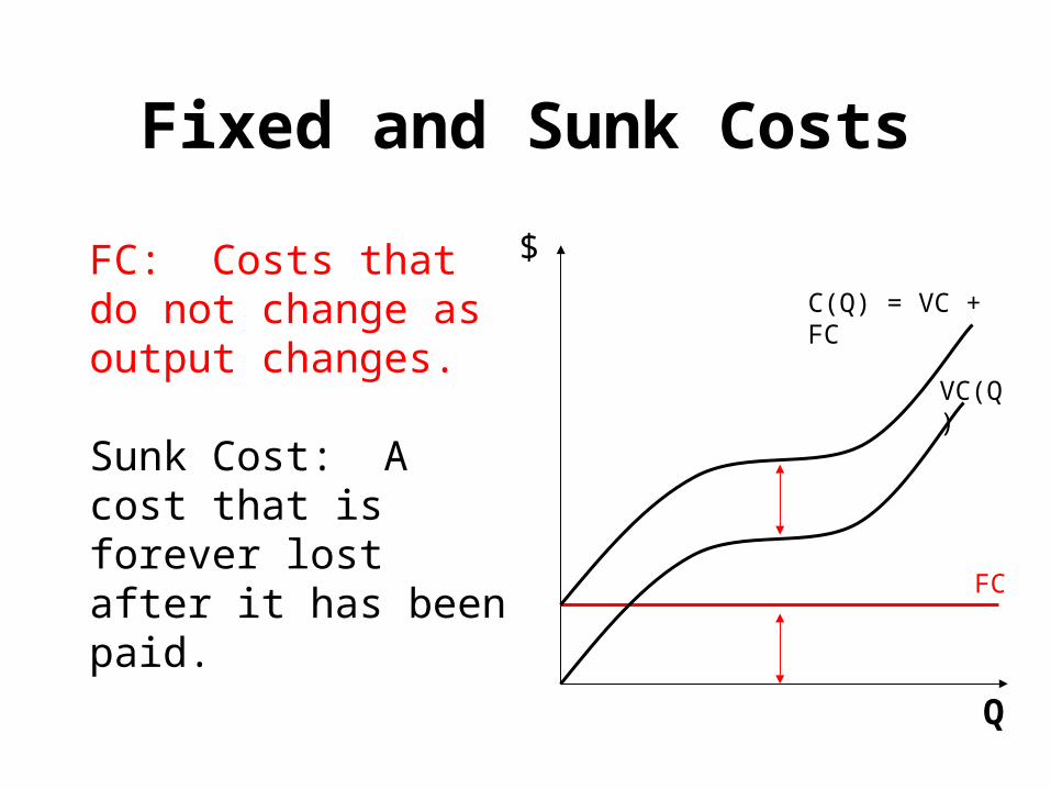
Fixed and Sunk Costs

FC: Costs that do not change as output changes.

Sunk Cost: A cost that is forever lost after it has been paid.

$

Q

FC

C(Q) = VC + FC

VC(Q)

Refer to Table 5.4 Page 181

Refer to Table 5.5 Page 1821-30

Some Definitions

Average Total CostATC = AVC + AFCATC = C(Q)/Q

Average Variable CostAVC = VC(Q)/Q

Average Fixed CostAFC = FC/Q

Marginal CostMC = C/Q

$

Q

ATCAVC

AFC

MC

MR

Fixed Cost

$

Q

ATC

AVC

MC

ATC

AVC

Q0

AFC Fixed Cost

Q0(ATC-AVC)

= Q0 AFC

= Q0(FC/ Q0)

= FC

Variable Cost

$

Q

ATC

AVC

MC

AVCVariable Cost

Q0

Q0AVC

= Q0[VC(Q0)/ Q0]

= VC(Q0)

$

Q

ATC

AVC

MC

ATC

Total Cost

Q0

Q0ATC

= Q0[C(Q0)/ Q0]

= C(Q0)

Total Cost

Cubic Cost Function

• C(Q) = f + a Q + b Q2 + cQ3

• Marginal Cost?– Memorize:

MC(Q) = a + 2bQ + 3cQ2

– Calculus:

dC/dQ = a + 2bQ + 3cQ2

An Example– Total Cost: C(Q) = 10 + Q + Q2

– Variable cost function:VC(Q) = Q + Q2

– Variable cost of producing 2 units:VC(2) = 2 + (2)2 = 6

– Fixed costs:FC = 10

– Marginal cost function:MC(Q) = 1 + 2Q

– Marginal cost of producing 2 units:MC(2) = 1 + 2(2) = 5

Economies of Scale

LRAC

$

Q

Economiesof Scale

Diseconomiesof Scale

Multi-Product Cost Function

• A function that defines the cost of producing given levels of two or more types of outputs assuming all inputs are used efficiently

• C(Q1, Q2): Cost of jointly producing two outputs.

• General multiproduct cost function 2

22

12121, cQbQQaQfQQC

Economies of Scope

• C(Q1, 0) + C(0, Q2) > C(Q1, Q2).

– It is cheaper to produce the two outputs jointly instead of separately.

• Example:– It is cheaper for Citycell to produce Internet

connections and Instant Messaging services jointly than separately.

Cost Complementarity

• The marginal cost of producing good 1 declines as more of good 2 is produced:

MC1Q1,Q2) /Q2 < 0.

• Example:– Bread and biscuits

Quadratic Multi-Product Cost Function

• C(Q1, Q2) = f + aQ1Q2 + (Q1 )2 + (Q2 )2

• MC1(Q1, Q2) = aQ2 + 2Q1

• MC2(Q1, Q2) = aQ1 + 2Q2

• Cost complementarity: a < 0

• Economies of scope: f > aQ1Q2

C(Q1 ,0) + C(0, Q2 ) = f + (Q1 )2 + f + (Q2)2

C(Q1, Q2) = f + aQ1Q2 + (Q1 )2 + (Q2 )2

f > aQ1Q2: Joint production is cheaper

A Numerical Example:

• C(Q1, Q2) = 100 – 1/2Q1Q2 + (Q1 )2 + (Q2 )2

• Cost Complementarity?

Yes, since a = -2 < 0

MC1(Q1, Q2) = -2Q2 + 2Q1

• Economies of Scope?

Yes, since 90 > -2Q1Q2

Conclusion

• To maximize profits (minimize costs) managers must use inputs such that the value of marginal of each input reflects price the firm must pay to employ the input.

• The optimal mix of inputs is achieved when the MRTSKL = (w/r).

• Cost functions are the foundation for helping to determine profit-maximizing behavior in future chapters.

Mid1 Answers

1. (a) p5; (b) p21; © p56; (d) p13; (e) p90; (f) p79.2. (a)p46; (b) p53(price floor, surplus).3. (a)p92; (b) -0.793; © -0.91(inelastic demand);

0.156(substitute, inelastic); 0.32(normal good, inelastic);0.13(positively related, inelastic).

4. (a) Px = 115 – ¼ Qxd; (b) 12,800; © 16,200; (d)

Consumer surplus decreases.5. (a) p=300; (b) p=200; Q=1000; © p=225; Q=1250.6. (a) No, demand is inelastic, revenue will fall; (b)

Income must rise by 22.22%; © Sale of shoes will increase by 2.25%.