1

Supplementary Information for

Bursting Drops in Solids Caused by High Voltages

Qiming Wang1, Zhigang Suo

2 and Xuanhe Zhao

1*

1 Soft Active Materials Laboratory, Department of Mechanical Engineering and Materials

Science, Duke University, Durham, NC 27708, USA.

2 School of Engineering and Applied Science, Kavli Institute for Nanobio Science and

Technology, Harvard University, Cambridge, MA 02138, USA.

* E-mail: xz69@duke.edu

2

Supplementary Figures

Supplementary Figure S1| The experimental setup for in situ observation of the

morphological evolution of conductive drops in a dielectric polymer. Drops of a conductive

liquid (10% wt NaCl solution) are trapped in a layer of a dielectric polymer. The radius of the

drop is much smaller than the thickness of the polymer. The polymer is then sandwiched

between two rigid insulating films, coated with transparent electrodes. The two electrodes were

then subject to a ramping voltage. The rigid films suppress overall deformation and electric

breakdown of the dielectric polymer, enabling in situ observation of the drops undergoing

morphological changes. The electric field far away from the drop is uniform and is regarded as

the applied electric field, E, on the drop.

3

Supplementary Figure S2| Evolution of a drop of a conductive liquid in a polymer observed

along the applied electric field. The radius of the center circle of the water drop decreases with

the increase of the electric field.

4

Supplementary Figure S3| Evolution of a drop of conductive liquid in a polymer under

oscillating electric field. In the first cycle, the drop deforms into a spheroid shape and reversibly

returns to the original spherical shape. In the second cycle, the drop forms a sharp tip and then

reversibly returns to the original spherical shape. In the third cycle, when the sharp tips open up,

the polymer around the apexes of the drop is fractured and the drop cannot return to its original

spherical shape. The ramping and retreating rate of the voltage is ±0.1kVs-1

. The scale bar is 100

µm and for all panels.

5

Supplementary Figure S4| Schematics of a drop in the polymer right before the onset of

sharp tips. Before the formation of the sharp tips, the drop deforms into the shape of a spheroid.

Due to the deformation of the drop, each apex of the drop is in a biaxially stretched state

with 1.13p

λ = .

6

Supplementary Figure S5| The nominal stress vs. stretch curve of the polymer used in the

current study under uniaxial tension. When the stretch is lower than 2.5, the polymer follows

the neo-Hookean law; and when the stretch exceeds 2.5, the polymer deviates from the neo-

Hookean law due to nonlinear stiffening.

7

Supplementary Figure S6| Finite-element calculation of the critical electric field for the

onset of a sharp tip in a biaxially stretched polymer with 1.13p

λ = . (a) The equipotential

contours in the polymer at the sharp-tip state calculated from the finite-element model. (b)

Potential-energy difference between the sharp-tip and flat states as a function of the local electric

field apex

E . As the local electric field reaches εµ /1.2 , the potential-energy difference reaches

zero and the sharp tip sets in.

8

Supplementary Figure S7| Calculation of the critical electric field for the onset of the sharp

tip in Figure 3a. (a) The polymer is under biaxial stretch of 04.1=pλ . (b) Potential-energy

difference between the sharp-tip and flat states as a function of the local electric field. As the

local electric field reaches 1.60 µ ε , the potential energy difference reaches zero and the sharp

tip sets in. Because the local electric field is 4.4 times of the applied electric field (Fig. 3d), the

critical applied field is 0.36 µ ε .

9

Supplementary Figure S8| The enhancement of electric field on the surface of two

conductive drops. (a) Schematic of two conductive drops of equal radius under an applied

electric field E along an arbitrary direction θ . (b) The maximum electric field on the surfaces of

the drop pairs varies with their distance aRd and the direction of the applied field θ 35. When

the distance decreases, the maximum field increases. A higher enhancement of the electric field

can give a lower critical electric field for the instability.

10

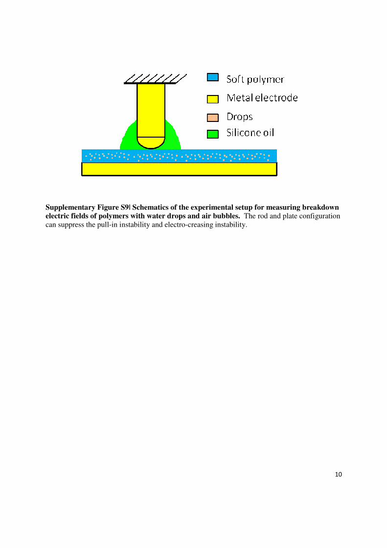
Supplementary Figure S9| Schematics of the experimental setup for measuring breakdown

electric fields of polymers with water drops and air bubbles. The rod and plate configuration

can suppress the pull-in instability and electro-creasing instability.