Burnout, NO, and Flame Characterization from an Oxygen ...

Brigham Young University Brigham Young University

BYU ScholarsArchive BYU ScholarsArchive

Theses and Dissertations

2015-05-01

Burnout, NO, and Flame Characterization from an Oxygen-Burnout, NO, and Flame Characterization from an Oxygen-

Enriched Biomass Flame Enriched Biomass Flame

Steven Andrew Owen Brigham Young University - Provo

Follow this and additional works at: https://scholarsarchive.byu.edu/etd

Part of the Mechanical Engineering Commons

BYU ScholarsArchive Citation BYU ScholarsArchive Citation Owen, Steven Andrew, "Burnout, NO, and Flame Characterization from an Oxygen-Enriched Biomass Flame" (2015). Theses and Dissertations. 5263. https://scholarsarchive.byu.edu/etd/5263

This Thesis is brought to you for free and open access by BYU ScholarsArchive. It has been accepted for inclusion in Theses and Dissertations by an authorized administrator of BYU ScholarsArchive. For more information, please contact [email protected], [email protected].

http://home.byu.edu/home/

http://home.byu.edu/home/

https://scholarsarchive.byu.edu/

https://scholarsarchive.byu.edu/etd

https://scholarsarchive.byu.edu/etd?utm_source=scholarsarchive.byu.edu%2Fetd%2F5263&utm_medium=PDF&utm_campaign=PDFCoverPages

http://network.bepress.com/hgg/discipline/293?utm_source=scholarsarchive.byu.edu%2Fetd%2F5263&utm_medium=PDF&utm_campaign=PDFCoverPages

https://scholarsarchive.byu.edu/etd/5263?utm_source=scholarsarchive.byu.edu%2Fetd%2F5263&utm_medium=PDF&utm_campaign=PDFCoverPages

mailto:[email protected],%[email protected]

Burnout, NO, and Flame Characterization from an

Oxygen-Enriched Biomass Flame

Steven Andrew Owen

A thesis submitted to the faculty of Brigham Young University

in partial fulfillment of the requirements for the degree of

Master of Science

Dale R. Tree, Chair Julie Crockett

David O. Lignell

Department of Mechanical Engineering

Brigham Young University

May 2015

Copyright © 2015 Steven Andrew Owen

All Rights Reserved

ABSTRACT

Burnout, NO, and Flame Characterization from an Oxygen-Enriched Biomass Flame

Steven Andrew Owen Department of Mechanical Engineering, BYU

Master of Science

Concern for the environment and a need for more efficient energy generation have sparked a growing interest throughout the world in renewable fuels. In order to reduce emissions that negatively contribute to global warming, especially CO2, enormous efforts are being invested in technologies to reduce our impact on the environment. Biomass is an option that is considered CO2 friendly due to the consumption of CO2 upon growth. Co-firing biomass with coal offers economic advantages because of reduced capital costs as well as other positive impacts, such as NOx and SOx emission reductions. However, due to the large average particle size of biomass, issues arise such as poor flame stability and poor carbon burnout. Larger particles can also result in longer flames and different heat transfer characteristics. Oxygen enrichment is being investigated as a possible solution to mitigate these issues and enable co-firing in existing facilities.

An Air Liquide designed burner was used in this work to explore the impact of oxygen enrichment on biomass flame characteristics, emissions, and burnout. Multiple biomass fuels were used (medium hardwood, fine hardwood, and straw) in conjunction with multiple burner configurations and operating conditions. Exhaust ash samples and exhaust NO were collected for various operating conditions and burner configurations. All operating parameters including O2 addition, swirl, and O2 location could be used to reduce LOI but whenever LOI was reduced, NO increased producing an NO-LOI trade-off.

Starting with high LOI, various parameters such as O2 addition and increased swirl could be used to reduce LOI with only small increases of NO. As O2 or swirl increased further, small decreases in LOI were obtained only with large increases in NO. This behavior was captured through NO-LOI trade-off curves where a given configuration or operating condition was deemed better when the curve was shifted toward the origin. Global enrichment or O2 addition to the secondary stream and O2 addition to the primary stream produced better trade-off results than center O2 injection. Straw produced NO-LOI trade-off curves just as the wood particles but the curve was shifted further from the origin, likely due to the higher nitrogen content of the straw. Flame characterization results showed that small amounts of O2 in the center improved flame attachment and stability while increasing flame temperature and pyrolysis rates.

Keywords: biomass combustion, hardwood biomass, wheat straw biomass, oxygen injection, oxygen enrichment, oxygen combustion, NO emission, carbon burnout

ACKNOWLEDGEMENTS

I am grateful for the opportunity I have had to attend Brigham Young University. My

academic experience has been a tremendous growing opportunity and I am grateful to be a part

of this great and well respected university.

I would like to thank Dr. Dale Tree for his support and encouragement throughout this

entire process. He has been an irreplaceable and enormous influence and mentor through his

knowledge and experience. I would like to thank my family for their love and support, especially

my wife, Chantelle, for her patience and understanding. I am grateful to my coworkers, Daniel

Tovar, Joshua Thornock, Daniel Ellis, and David Ashworth, who have assisted in the operation

of the Burner Flow Reactor and the collection of data. Their support and experience have been

particularly helpful. Yuan Xue, Kenneth Kaiser, Hwanho Kim, Remi Tsiavi and Louis, all from

Air Liquide, have each been more than helpful in supporting this project. Also, Air Liquide has

been an amazing sponsor for the financial support of this work, which is greatly appreciated.

iv

TABLE OF CONTENTS

List of Tables ...............................................................................................................................vii

List of Figures ............................................................................................................................... ix

Nomenclature .............................................................................................................................xiii

1 Introduction ........................................................................................................................... 1

1.1 Objectives ....................................................................................................................... 3

1.2 Scope ............................................................................................................................... 3

2 Background ........................................................................................................................... 5

2.1 Formation of Nitric Oxides ............................................................................................. 5

2.2 Particle Burnout and Loss on Ignition (LOI) .................................................................. 8

2.3 Swirl Stabilized Solid Fuel Flames ............................................................................... 10

3 Literature Review ............................................................................................................... 15

3.1 Biomass Swirl Assisted Flames .................................................................................... 15

3.2 Burner Co-Firing ........................................................................................................... 16

3.3 Oxygen Usage in Biomass Flames ............................................................................... 18

3.3.1 Oxy-Fuel Combustion (OFC) ................................................................................... 18

3.3.2 Enriched Air Combustion (EAC) .............................................................................. 19

3.3.3 Oxygen Injection Combustion (OIC) ........................................................................ 20

3.4 Summary and Objective ................................................................................................ 22

4 Experimental Setup and Method ....................................................................................... 23

4.1 BYU Combustion Facility ............................................................................................ 23

4.2 Fuel Analyses ................................................................................................................ 25

4.3 Burner Configurations and Operating Conditions ........................................................ 27

4.4 NO Measurements ........................................................................................................ 31

4.5 Ash Collection and Loss on Ignition ............................................................................ 32

v

5 NO and LOI Results and Discussion ................................................................................. 35

5.1 Nitric Oxide Emission (NO) ......................................................................................... 35

5.1.1 NO vs. Swirl .............................................................................................................. 35

5.1.2 NO vs. O2 .................................................................................................................. 38

5.1.3 NO vs. Primary Air ................................................................................................... 39

5.1.4 NO Summary ............................................................................................................ 40

5.2 Loss on Ignition (LOI) .................................................................................................. 41

5.2.1 LOI vs. Swirl ............................................................................................................. 41

5.2.2 LOI vs. O2 ................................................................................................................. 42

5.2.3 LOI vs. Primary Air .................................................................................................. 43

5.2.4 LOI Summary ........................................................................................................... 44

5.3 NO vs. LOI Trade-off ................................................................................................... 44

5.3.1 Swirl .......................................................................................................................... 45

5.3.2 Primary Air ............................................................................................................... 50

5.3.3 Burner Configuration ................................................................................................ 52

5.3.4 Variable vs. Constant Secondary Flow Rate ............................................................. 53

5.3.5 O2 Location ............................................................................................................... 54

5.3.6 NO vs. LOI Summary and Discussion ...................................................................... 56

5.4 NO-LOI Data for Straw and Fine Biomass .................................................................. 60

5.4.1 Straw NO-LOI for Variable Swirl ............................................................................ 60

5.4.2 Straw NO-LOI for Variable O2 Location .................................................................. 61

5.4.3 Straw Burned in Various Burner Configurations ...................................................... 63

5.4.4 Fine Hardwood Results ............................................................................................. 64

5.4.5 Fuel Comparisons ..................................................................................................... 65

6 Scaling Laws and Correlation for NO and LOI ............................................................... 69

vi

6.1 A Phenomenological Flame Model .............................................................................. 69

6.1.1 Lift-Off and Flame Length Measurements ............................................................... 72

6.1.2 Flame Length Model ................................................................................................. 74

6.2 Flame Length Model – Measurement Comparison ...................................................... 76

7 Summary and Conclusions ................................................................................................. 81

References .................................................................................................................................... 85

APPENDIX A: Air Liquide Burner Swirl ................................................................................ 89

A.1 Swirl Calculations ......................................................................................................... 89

A.2 Axial Profile Data ......................................................................................................... 92

APPENDIX B: Data From Reactor........................................................................................... 97

B.1 Uncertainty Analysis ..................................................................................................... 97

B.2 Extra Plots ..................................................................................................................... 99

B.3 All Data ....................................................................................................................... 102

APPENDIX C: Fourier Transform Infrared Spectrometer ................................................. 115

vii

LIST OF TABLES

Table 4.1: Proximate and ultimate analysis (as received), heating value, and mean particle size of the three biomass fuels used .......................................................................................26

Table 4.2: Relative diameters of each of the tubes in the Air Liquide Burner ..............................28

Table 4.3: Test matrix of burner geometry configurations, flow rates, and condition nomenclature ..........................................................................................................................29

Table 4.4: LOI measurements from two different fuels and temperatures ....................................33

Table 5.1: Summary of uncertainty in the measurements taken ....................................................37

Table A.1: Selected dimensions of Air Liquide burner .................................................................90

Table A.2: Multiple rod rotations matched with corresponding theoretical secondary swirl numbers for the four possible configurations ........................................................................91

Table B.1: Summary of uncertainty in the measurements taken ...................................................99

Table B.2: Medium hardwood data with oxygen in the center tube, recessed 76 mm, using configuration 1S2L3L ..........................................................................................................102

Table B.3: Medium hardwood data with oxygen in the annulus, fuel in the center tube, recessed 76 mm, using configuration 1L2L3L ....................................................................103

Table B.4: Medium hardwood data with oxygen in the center, using configuration 1S2L3L ....103

Table B.5: Medium hardwood data with oxygen added to the secondary, center tube recessed 10 mm, using configuration 1S2L3L.....................................................................104

Table B.6: Medium hardwood data with oxygen in the center using configuration 1S2L3L .....105

Table B.7: Medium hardwood data with oxygen in the center using configuration 1M2L3L with bluff-body ....................................................................................................................106

Table B.8: Medium hardwood data with oxygen in the center using configuration 1S2S3S ......106

Table B.9: Wheat straw data with oxygen in the center using configuration 1S2L3L ................107

Table B.10: Wheat straw data with oxygen in the center using configuration 1S2L3S ..............108

Table B.11: Wheat straw data with oxygen in the center, tube recessed 25 mm, using configuration 1S2L3S ..........................................................................................................109

Table B.12: Medium hardwood data with oxygen in the center, tube recessed 25 mm, using configuration 1S2L3S ..........................................................................................................109

viii

Table B.13: Hardwood data under over-fire air conditions, 52 kg/hr tertiary air, oxygen in the center, center tube flush, using configuration 1S2L3L ..................................................110

Table B.14: Medium hardwood data with oxygen in the center, center tube flush, using configuration 1L2L3L ..........................................................................................................110

Table B.15: Medium hardwood data with oxygen in four-hole lance, center tube flush, using configuration 1M2L3L ...............................................................................................111

Table B.16: Medium hardwood data with oxygen in the center tube being premixed using eight-hole lance, using configuration 1M2L3L ...................................................................112

Table B.17: Medium hardwood data with oxygen in the center tube being premixed using six-hole lance, using configuration 1S2L3L ........................................................................113

Table B.18: Fine hardwood data with oxygen in the center tube being premixed using six-hole lance, using configuration 1S2L3L ..............................................................................113

ix

LIST OF FIGURES

Figure 2.2: Four different types of swirled flames as designated by the IFRF: (a) Type 0, (b) Type 1, (c) Type 2, and (d) Type 3 ..................................................................................11

Figure 2.3: Swirled burner cross-sectional diagram depicting a fuel rich region that is surrounded by a recirculating secondary flow .......................................................................12

Figure 4.4: Schematic of various oxygen lances used in data collection; tubes are named from left to right: open, bluff-body, four-hole, six-hole, and eight-hole ...............................30

Figure 5.1: NO (ppm) vs. Swirl at varying oxygen flow rates, configuration 1S2L3L, medium hardwood, constant secondary air for (a) Global Enrichment and (b) Center Injection .................................................................................................................................36

Figure 5.2: NO (ppm) vs. Swirl for various burner configurations, no oxygen, medium hardwood, and constant secondary air ...................................................................................37

Figure 5.3: NO (ppm) vs. Oxygen Flow Rate (kg/hr) for four configurations at maximum swirl, medium hardwood, center injection, and constant secondary air ................................38

Figure 5.4: NO (ppm) vs. Oxygen Flow Rate (kg/hr) and varying swirl for the medium hardwood, configuration 1S2L3L, center injection, tube 1 extended 70 mm ........................39

Figure 5.5: NO (ppm) vs. Primary Air Flow Rate (kg/hr) for the medium hardwood, configuration 1S2L3L ............................................................................................................40

Figure 5.6: LOI vs. Swirl at five flow rates of oxygen in the center, configuration 1S2L3L, medium hardwood, and constant secondary air for (a) Global Enrichment and (b) Center Injection ......................................................................................................................41

Figure 5.7: LOI vs. Swirl for various burner configurations, no oxygen, medium hardwood, and constant secondary air .....................................................................................................42

Figure 5.8: LOI vs. Oxygen Flow Rate (kg/hr) for four configurations at maximum swirl, medium hardwood, center injection, and constant secondary air ..........................................43

Figure 5.9: LOI vs. Primary Air Flow Rate (kg/hr) for the medium hardwood, configuration 1S2L3L ............................................................................................................44

Figure 5.10: NO (ppm) vs. LOI for three swirl values at five oxygen flow rates (0, 2, 4, 6, 8 kg/hr), configuration 1S2L3L, medium hardwood, constant secondary air for (a) Global Enrichment and (b) Center Injection ..........................................................................45

Figure 5.11: NO (ppm) vs. LOI for three swirl values at five oxygen flow rates (0, 2, 4, 6, 8 kg/hr), configuration 1L2L3L, medium hardwood, constant secondary air for (a) Center Injection and (b) Fuel in Center .................................................................................46

x

Figure 5.12: NO (ppm) vs. LOI for three swirl values at five oxygen flow rates (0, 2, 4, 6, 8 kg/hr), center injection, 25 mm recess, configuration 1S2L3S, medium hardwood, constant primary air (24 kg/hr), and constant secondary air ..................................................47

Figure 5.13: NO (ppm) vs. LOI for four type of oxygen injection techniques, configuration 1M2L3L, medium hardwood, flush location unless otherwise specified, and constant secondary air ..........................................................................................................................48

Figure 5.14: NO (ppm) vs. LOI for three levels of extension of the oxygen lance, center injection, configuration 1S2L3L, medium hardwood, and constant secondary air ...............49

Figure 5.15: NO (ppm) vs. LOI for five heights of extension, 4 kg/hr oxygen flow rate center injection, medium hardwood, constant secondary air for (a) Configuration 1S2S3S and (b) Configuration 1M2L3L ................................................................................50

Figure 5.16: NO (ppm) vs. LOI for varying primary flow rates, no oxygen introduced, medium hardwood, configuration 1S2L3L ............................................................................51

Figure 5.17: NO (ppm) vs. LOI for two primary flow rates, varying amounts of premixed oxygen (0, 4, and 8 kg/hr), medium hardwood, configuration 1S2L3L ................................52

Figure 5.18: NO (ppm) vs. LOI at maximum swirl for four different configurations, varying amounts of oxygen flow rates, center injection, medium hardwood, and constant secondary air ............................................................................................................53

Figure 5.19: NO (ppm) vs. LOI for varied secondary air, medium hardwood, configuration 1S2L3L with (a) Global Enrichment and (b) Center Injection ..............................................54

Figure 5.20: NO (ppm) vs. LOI for two oxygen addition techniques, global enrichment and air addition, configuration 1S2L3L, and medium hardwood .................................................55

Figure 5.21: NO (ppm) vs. LOI for five oxygen addition techniques, configuration 1S2L3L, and medium hardwood ............................................................................................56

Figure 5.23: NO (ppm) vs. LOI at eight different type of operating conditions for the medium hardwood and configuration 1S2L3L ......................................................................59

Figure 5.24: NO (ppm) vs. LOI at three different swirl values for various oxygen flow rates, center injection, configuration 1S2L3S, 25 mm recess, wheat straw biomass, and constant secondary air .....................................................................................................61

Figure 5.25: NO (ppm) vs. LOI at two oxygen injection locations (Global and Center), varying amounts of O2 flow rate, wheat straw biomass, maximum swirl, for burner configurations (a) 1S2L3S and (b) 1S2L3L ...........................................................................62

Figure 5.26: NO (ppm) vs. LOI at three different center tube extension heights, three O2 flow rates (0, 4, and 8 kg/hr) in tube 1, wheat straw biomass, maximum swirl, for burner configurations (a) 1S2L3S and (b) 1S2L3L ...............................................................63

xi

Figure 5.27: NO (ppm) vs. LOI at their respective maximum swirl value for various oxygen flow rates, center injection, wheat straw biomass, and constant secondary air ........64

Figure 5.28: NO (ppm) vs. LOI for three swirl values at varying oxygen flow rates in six-hole lance, flush, configuration 1S2L3L, fine hardwood, and constant secondary air ..........65

Figure 5.29: NO (ppm) vs. (a) LOI and (b) Burnout at the respective maximum swirl value for various oxygen flow rates, configuration 1S2L3L, and constant secondary air ..............66

Figure 5.30: NO (ppm) vs. (a) LOI and (b) Burnout for both medium and fine hardwood at various oxygen flow rates using the six-hole oxygen lance, configuration 1S2L3L, and constant secondary air .....................................................................................................67

Figure 5.31: NO (ppm) vs. LOI at three swirl values for various oxygen flow rates, medium and fine hardwood, configuration 1S2L3L, and constant secondary air .................68

Figure 6.2: NO (ppm) vs. LOI at three different swirl settings, varying flow rates of oxygen, center injection, medium hardwood, for burner configurations (a) 1S2L3S, (b) 1S2L3L and (c) 1L2L3L ..................................................................................................73

Figure 6.3: Calculated Flame Length (m) vs. Visually Estimated Length (m) for all data collected separated by fuel .....................................................................................................76

Figure 6.4: Oxygen Flow Rate (kg/hr) vs. Flame Length (m) for three oxygen addition techniques, configuration 1S2L3L, medium hardwood, and constant secondary air ............77

Figure 6.5: (a) NO (ppm) and (b) LOI vs. Flame Length (m) for five oxygen addition techniques, medium hardwood, and configuration 1S2L3L ..................................................78

Figure 6.6: (a) NO (ppm) and (b) LOI vs. Flame Length (m) for all medium hardwood data collected separated by configuration......................................................................................79

Figure 6.7: (a) NO (ppm) and (b) LOI vs. Flame Length (m) for all wheat straw data collected separated by configuration......................................................................................79

Figure A.2: Velocity (m/s) vs. Distance from Annular Pipe (cm) for configuration 2L3S and the following conditions: (a) Axial 158 kg/hr, (b) Tangential 158 kg/hr, (c) Axial 170 kg/hr, and (d) Tangential 170 kg/hr ................................................................................93

Figure A.3: Velocity (m/s) vs. Distance from Annular Pipe (cm) for configuration 2L3L and the following conditions: (a) Axial 158 kg/hr, (b) Tangential 158 kg/hr, (c) Axial 170 kg/hr, and (d) Tangential 170 kg/hr ................................................................................94

Figure A.4: Corrected Velocity (m/s) vs. Distance from Annular Pipe (cm) for configuration 2L3S and the following conditions: (a) Axial 158 kg/hr, (b) Tangential 158 kg/hr, (c) Axial 170 kg/hr, and (d) Tangential 170 kg/hr ...............................................95

xii

Figure A.5: Corrected Velocity (m/s) vs. Distance from Annular Pipe (cm) for configuration 2L3L and the following conditions: (a) Axial 158 kg/hr, (b) Tangential 158 kg/hr, (c) Axial 170 kg/hr, and (d) Tangential 170 kg/hr ...............................................96

Figure B.1: NO (ppm) vs. LOI showing (a) All Hardwood Data and configurations (b) 1S2L3L, (c) 1S2S3S, (d) 1S2L3S, (e) 1M2L3L, and (f) 1L2L3L .......................................100

Figure B.2: NO (ppm) vs. LOI showing (a) All Straw Data and configurations (b) 1S2L3S, (c) 1S2L3L, and (d) 1M2L3S ..............................................................................................101

xiii

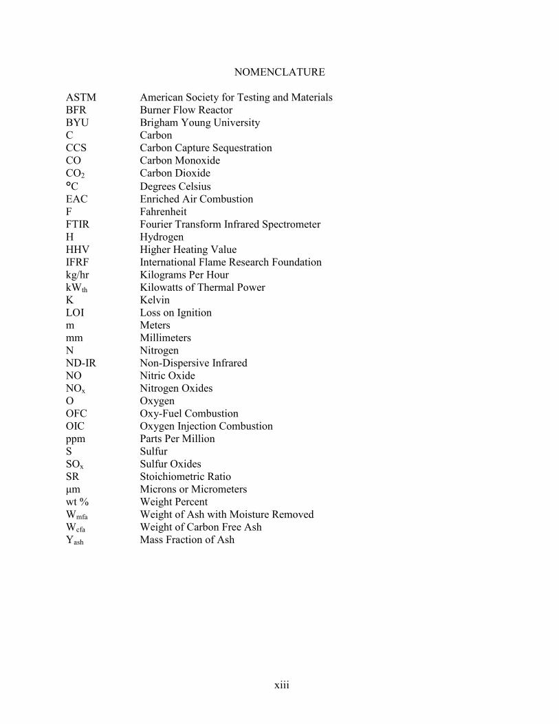
NOMENCLATURE

ASTM American Society for Testing and Materials BFR Burner Flow Reactor BYU Brigham Young University C Carbon CCS Carbon Capture Sequestration CO Carbon Monoxide CO2 Carbon Dioxide °C Degrees Celsius EAC Enriched Air Combustion F Fahrenheit FTIR Fourier Transform Infrared Spectrometer H Hydrogen HHV Higher Heating Value IFRF International Flame Research Foundation kg/hr Kilograms Per Hour kWth Kilowatts of Thermal Power K Kelvin LOI Loss on Ignition m Meters mm Millimeters N Nitrogen ND-IR Non-Dispersive Infrared NO Nitric Oxide NOx Nitrogen Oxides O Oxygen OFC Oxy-Fuel Combustion OIC Oxygen Injection Combustion ppm Parts Per Million S Sulfur SOx Sulfur Oxides SR Stoichiometric Ratio μm Microns or Micrometers wt % Weight Percent Wmfa Weight of Ash with Moisture Removed Wcfa Weight of Carbon Free Ash Yash Mass Fraction of Ash

1

1 INTRODUCTION

Concern for the environment and the need for efficient energy generation have sparked a

growing interest throughout the world in renewable fuels and options geared to secure the future

of clean energy. In recent years, there has been an increasing effort to reduce emissions that are

known to negatively contribute to global climate change. One of the main contributors to global

climate change is carbon dioxide (CO2) emissions. In 2012, CO2 accounted for 82% of all U.S.

greenhouse gas emissions from human activities with combustion of fossil fuels for energy and

transportation noted as the main source for CO2 emissions [1]. Power plants and other

combustion facilities often have large CO2 emissions because CO2 is the end product for fuels

containing carbon. While regulations on the emission of greenhouse gases continue to rise,

enormous efforts have been invested into technologies that reduce CO2. Viable options include

various fuels that are more CO2 neutral. One way CO2 emissions from power generation can be

reduced, both effectively and inexpensively, is to substitute coal with biomass or by burning the

two simultaneously in a process known as co-firing [2].

Biomass is often considered relatively CO2 neutral due to the biological nature of

biomass consuming CO2 during photosynthesis [3]. Co-firing biomass with coal reduces CO2

emissions and often simultaneously produces other positive impacts, such as emission reductions

of nitrogen oxides (NOx) and sulfur oxides (SOx) [4]. A review of over 100 successful field

demonstrations in 16 countries with various combinations of coal and biomass using every major

type of boiler have identified several challenges including fuel preparation, storage, and delivery,

2

potential increases in corrosion, ash deposition issues, carbon burnout, ash utilization and overall

cost [2, 5, 6]. When roller mills used for coal are instead used for biomass, it is difficult to

produce the same small particle size. The cost of grinding biomass to the same size as coal is

prohibitive. Due to its properties, such as shape and density, biomass exhibits rapid oxidation

and combustion rates. However, these rates are not rapid enough to make up for the increased

particle size resulting in unburned carbon and fouling as problematic areas for boilers converted

to or co-firing biomass. Excessive moisture along with excessive particle size can pose a

challenge for fuel conversion efficiency [3, 4].

Although biomass can reduce NOx and SOx emissions these pollutants are still a matter of

concern and need to be controlled in biomass combustion. NOx and SOx are harmful to both

health and the environment. NOx emissions can result in negative respiratory effects from

various amounts of exposure and concentration levels. It negatively affects the environment by

contributing to acid deposition and forming particulate matter. It is important to maintain low

levels of NO in order to protect the environment and ensure safe and healthy living conditions

[7]. SOx emissions also have negative respiratory effects as they react and form particulate

matter with other compounds. Fossil fuel combustion (73%) and other industrial facilities (20%)

account for 93% of SO2 emissions [8]. NOx emission is typically more prevalent than SOx in

biomass combustion and will be one of the main focus points of this work.

Studies have shown that an oxygen enriched environment during biomass combustion

can improve mass loss rates and particle burnout [9, 10]. While oxygen enrichment may increase

particle burnout, NO formation can be negatively affected. Bool et al. [11, 12] made several

observations where oxygen was injected into coal flames and concluded certain methods of

oxygen injection can be successfully implemented for NO reduction. Oxygen enrichment is

3

being investigated as a possible solution to mitigate emission and particle burnout issues and thus

enable co-firing in many existing facilities. This work explores the possibility of using oxygen to

improve carbon burnout without significantly increasing NO emissions.

1.1 Objectives

The objective of this work is to explore the design space of oxygen injection in a swirl

stabilized burner for the reduction of unburned carbon and improvement of flame stability

without increasing NOx emissions. Data will be collected on a 150 kWth laboratory scale reactor

and will include the measurement of carbon burnout and exhaust emissions of NO, CO, CO2, and

O2 as well as visual flame characterization of flame length and flame lift-off. Three fuels,

medium hardwood, fine hardwood, and wheat straw, will be used as representative biomass

particles. The data will be used to explore an empirical characterization of the flame and

determine the optimal conditions for which oxygen enrichment will simultaneously improve

burnout and reduce NO emissions.

1.2 Scope

This work will focus on the impact of various design parameters on exhaust products,

primarily NOx and particle loss on ignition. Flame characterization will be done by visual

observation. Detailed mapping of flame species, burnout, and temperature will not be completed

for this work. The work will also be limited to three fuels; medium hardwood, fine hardwood,

and straw. Computational work will include the application of existing scaling laws to the

current work and the development of those scaling laws but will not include comprehensive

combustion modeling.

5

2 BACKGROUND

Information needed for understanding the methods used as well as the results and their

significance is presented in this chapter, including a discussion of NO formation, the process of

carbon burnout, and the definition of swirl.

2.1 Formation of Nitric Oxides

NOx is the term used for the combined pollutants of NO and NO2. In coal combustion the

primary component of NOx is NO. The formation of NO for biomass combustion follows three

main chemical pathways often referred to as thermal, prompt, and fuel NO. An understanding of

these pathways provides the background necessary for the interpretation of the results to be

presented and an understanding of how to produce minimum NOx emissions.

Thermal NOx is strongly dependent on temperature, being unimportant below

temperatures of 1800 K. The extended Zeldovich mechanism, shown in Equations 2.1 through

2.3, provides the reactions and species involved [13]. It has been noted, however, that timescales

of the thermal mechanism are much slower than that of fuel oxidation processes, and has

therefore been demonstrated that NO is formed in post flame gas regions. In addition, previous

work from the reactor used in this work has shown that temperatures are above 1800 K solely in

the region of the flame, and therefore this path for NO formation is assumed negligible in these

experiments [14].

6

𝑂 + 𝑁2 ⇔ 𝑁𝑂 + 𝑁 (2.1)

𝑁 + 𝑂2 ⇔ 𝑁𝑂 + 𝑂 (2.2)

𝑁 + 𝑂𝑂 ⇔ 𝑁𝑂 + 𝑂 (2.3)

Prompt NO is rapidly formed during the combustion of hydrocarbons by the Fenimore

mechanism, shown in Equations 2.4 and 2.5 [13]. For prompt NO, hydrocarbon radicals react

with nitrogen and result in cyanides. These cyanide compounds convert to intermediate

compounds and can ultimately result in NO. This pathway of NO formation can occur more

rapidly than the time needed for thermal NOx, thus earning its name.

𝐶𝑂 + 𝑁2 ⇔ 𝑂𝐶𝑁 + 𝑁 (2.4)

𝐶 + 𝑁2 ⇔ 𝐶𝑁 + 𝑁 (2.5)

Fuel NO is the third main path and the major contributor of NO in pulverized biomass

and coal combustion [15]. Biomass and coal contain nitrogen in their molecular structure which

is released as volatiles, or light gases, when the fuel particles are heated. The process of volatiles

being released is called devolatilization. Nitrogen in biomass volatiles is typically released as

ammonia (NH3), whereas with coal a mixture of hydrogen cyanide (HCN) and NH3 is more

common. These volatiles can then oxidize and form NO, as shown in the sequence of Equations

2.6 through 2.9 [13].

𝑂𝐶𝑁 + 𝑂 ⇔ 𝑁𝐶𝑂 + 𝑂 (2.6)

𝑁𝐶𝑂 + 𝑂 ⇔ 𝑁𝑂 + 𝐶𝑂 (2.7)

𝑁𝑂 + 𝑂 ⇔ 𝑁 + 𝑂2 (2.8)

𝑁 + 𝑂𝑂 ⇔ 𝑁𝑂 + 𝑂 (2.9)

7

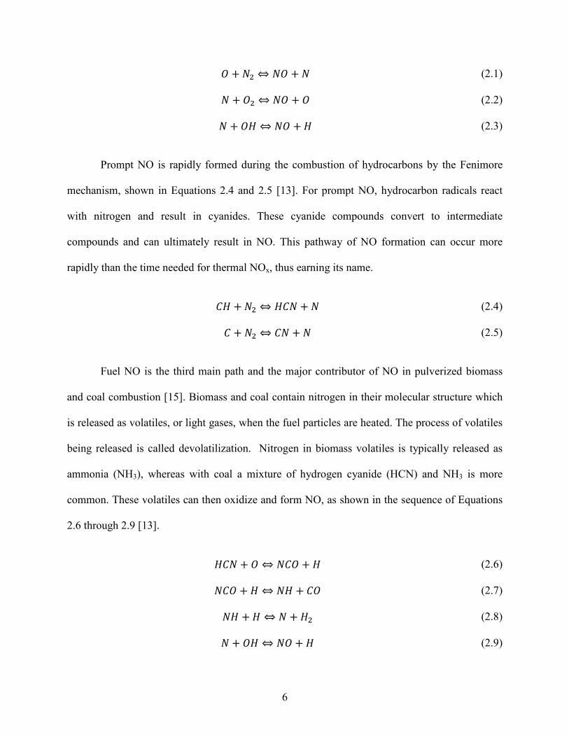
The sequence shown is not the only method for fuel nitrogen conversion to NO but

represents one of the primary pathways. Significant nitrogen products include NO, NO2, and N2.

Figure 2.1 is a diagram depicting how nitrogen in the fuel can be converted to either NO or N2

depending on the local stoichiometry. Intermediates such as NH3 and HCN can either react with

oxidizing species to produce NO or they can react with NO to produce N2 under reducing

environments. It should be noted, however, that NO cannot be eliminated entirely in this way. A

fuel rich region, essential for NO reduction, must be maintained at an optimal oxidizer to fuel

ratio to enable NO reduction to be a maximum.

Reburning is a term introduced by Wendt [16, 17] which refers to the addition of fuel to

produce a fuel rich zone wherein NO is reduced to N2. The stoichiometric ratio (SR) for

reburning appears to have an optimum in the range of 0.65 to 0.85 depending on the fuel and

temperature [18]. These same reburning reactions are present in the fuel rich recirculation zone

of a swirled burner and therefore there should also be an optimal SR within this fuel rich zone for

NO reduction.

Figure 2.1: Reaction mechanism converting fuel nitrogen to NO and N2

8

2.2 Particle Burnout and Loss on Ignition (LOI)

Solid fuel particles have two main types of reaction, volatile combustion and char

oxidation. Volatile combustion was discussed briefly with NO formation where light gases react

with oxygen. Char oxidation, or particle burnout, is a process that occurs after the volatiles have

been released and when carbon remaining in the particle reacts with surrounding oxygen. At the

particle surface, carbon can react with an oxidizer via the global reactions shown in Equations

2.10 through 2.13 [19].

𝐶 + 𝑂2 ⇔ 𝐶𝑂2 (2.10)

2𝐶 + 𝑂2 ⇔ 2𝐶𝑂 (2.11)

𝐶 + 𝐶𝑂2 ⇔ 2𝐶𝑂 (2.12)

𝐶 + 𝑂2𝑂 ⇔ 𝐶𝑂 + 𝑂2 (2.13)

The primary product at the surface of the particle is CO. The CO will diffuse away from

the particle and can react further with O2, shown in Equation 2.14 [19]. These equations indicate

that if particles have not been completely consumed, or oxidized, it may result in a high level of

CO in the exhaust gas.

𝐶𝑂 + 1

2𝑂2 ⇔ 𝐶𝑂2 (2.14)

The final product of the carbon in char is CO2. Some of the factors that control the rate of

char oxidation, or the rate of the consumption of the carbon, are temperature, pressure, and

particle size. When the temperature and pressure are high and the particle size is large the

diffusion of oxygen to the particle limits the rate of the chemical reaction. This means the

chemical reaction happens as fast as oxygen is able to get to the particle and is referred to as a

9

diffusion controlled reaction. When the temperature and pressure are low and the particle size is

small the rate at which the carbon is consumed is limited by the chemical reaction, referred to as

a kinetically controlled reaction. Kinetically controlled reactions do not have a dependence on

the oxygen concentration. For diffusion controlled reactions an increase of oxygen would

increase the rate at which the char particle is consumed, whereas kinetically controlled reactions

would be not be as greatly impacted by the increase. It is common for both diffusion and kinetics

to play a role in the rate of char oxidation depending on the location of the particle and the time-

temperature history.

Loss on ignition (LOI) is an important indicator of combustion efficiency. It is a measure

of the amount of mass removed from a particle when completely oxidized. The majority of the

mass remaining in coal and biomass ash is carbon although other trace elements may also

contribute to mass loss.

To obtain an LOI measurement, ash is placed in a crucible, weighed, heated to remove

moisture, and then weighed again. Once the moisture free weight is established, the ash is then

subjected to a higher temperature that consumes the remaining carbon, and the mass of the

remaining ash is then compared to the mass of the moisture free ash. If there is only a small

amount of carbon remaining, the ash will lose only a small amount of mass and will be low in

LOI. A larger amount of carbon in the ash will lose more mass through this process and the LOI

value will be higher. Section 4.5 contains a detailed process used to measure LOI for this work.

The carbon content in the ash can be used as a measure of how much energy is not released upon

ignition and reaction. It would be desirable that all the carbon in ash is consumed during the

combustion process and that a small amount of carbon remain in the ash.

10

In addition to revealing combustion efficiency, ash waste from coal is beneficial as an

ingredient in concrete and can even contribute to a significant percentage of concrete in roads,

but this is only the case if the carbon content of the ash is low. If there is too much carbon in the

ash, more than 6% LOI, then the ash must be disposed in a landfill rather than being reused in

another form [20].

2.3 Swirl Stabilized Solid Fuel Flames

Swirl is an important parameter used to maintain a stable flame that is reduced in size

with increased intensity. Swirl is defined as the ratio of axial flux of tangential momentum to

axial flux of axial momentum times the nozzle radius [21]. Equations for the calculation of swirl

are shown in Appendix A.1. According to the International Flame Research Foundation, IFRF,

there are four classifications of flame types [22]. Each of these is seen in Figure 2.2. Type 0

corresponds to external recirculation. In this flame type there may be some outer rotation, but

little swirl is present. Flame type 1 is internal recirculation with fuel jet penetration. This flame is

stronger than type 0 and has a closed recirculation zone. Flame type 1 is typical of a

characteristic flame as seen in this work. Flame type 2 is where the fuel jet stagnates and spreads

in the internal recirculation zone. This recirculation remains closed with no jet penetration and is

typically a very short intense flame. Lastly, flame type 3 is the same as flame type 1, but with a

second downstream internal recirculation zone. Flame type 3 has high confinement of the flame.

As swirl increases the flame type moves from type 0 to type 3.

Swirl not only decreases the length of the flame, but also can reduce flame lift off and

improve flame stability. Swirl can be used to improve NO and/or LOI emissions. Swirl is created

by adding tangential flow to an axial flow component. When the air exits the tube, the

momentum caused by the swirling flow causes air to move outward and produces a low pressure

11

region in the center. This low pressure in the reactor draws combustion products towards the

burner enabling devolatilization of the solid fuel, facilitating ignition of volatiles and the creating

of a fuel rich region through which the fuel and recirculated products must pass.

(a) Type 0

(b) Type 1

(c) Type 2

(d) Type 3

Figure 2.2: Four different types of swirled flames as designated by the IFRF: (a) Type 0, (b) Type 1, (c) Type 2, and (d) Type 3

12

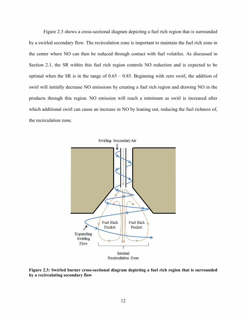
Figure 2.3 shows a cross-sectional diagram depicting a fuel rich region that is surrounded

by a swirled secondary flow. The recirculation zone is important to maintain the fuel rich zone in

the center where NO can then be reduced through contact with fuel volatiles. As discussed in

Section 2.1, the SR within this fuel rich region controls NO reduction and is expected to be

optimal when the SR is in the range of 0.65 – 0.85. Beginning with zero swirl, the addition of

swirl will initially decrease NO emissions by creating a fuel rich region and drawing NO in the

products through this region. NO emission will reach a minimum as swirl is increased after

which additional swirl can cause an increase in NO by leaning out, reducing the fuel richness of,

the recirculation zone.

Figure 2.3: Swirled burner cross-sectional diagram depicting a fuel rich region that is surrounded by a recirculating secondary flow

13

Swirl also has an impact on carbon burnout. The shortened flame produced by increased

swirl provides an increased residence time for particles in the post volatile flame region. Having

a large amount of swirl can also entrain solid fuel particles effectively into regions of lower axial

velocity increasing their residence time. Decreasing swirl typically elongates the flame allowing

particles to travel toward the exhaust exit within a fuel rich region without access to burnout

oxygen.

It is therefore important to have an appropriate swirl value that is both beneficial to NOx

emission and carbon burnout. In this research effort, oxygen is added in various locations and

amounts to flames of varying swirl to determine if the oxygen can be beneficial to burnout

without negatively impacting NO emission. One scenario where this might be possible would be

the use of oxygen to increase flame temperature and devolatilization rates so that the optimal SR

in the fuel rich region can be reached in shorter distances and allow increased burnout.

15

3 LITERATURE REVIEW

This chapter provides a review of previous research efforts in the area of oxygen injection

combustion in biomass flames. This review first provides an explanation and examples of several

ways that biomass can be burned and ways in which oxygen can be used in conjunction with

biomass for combustion, but the specific topic of the review is limited to oxygen being injected

into biomass flames to improve combustion.

3.1 Biomass Swirl Assisted Flames

Although there are several methods used to burn fuels in boilers, one of the most

prominent is pulverized coal transported in primary air injected into swirled air (secondary air).

The swirl creates the recirculation of hot product gases that ignite and stabilize the flame. Studies

have shown that swirl is effective in producing short, intense flames that increase the residence

times of solid fuel particles [22]. Swirl was initially introduced to burners for flame stability and

to decrease boiler size. Later, swirl and secondary flow was decreased to produce a near burner

fuel rich zone followed by tertiary air injection. This staged air is effective at NOx reduction and

is referred to as a low NOx burner. Low NOx burners can reduce NOx up to 50-60% but have

flames one and a half times longer than previous burners [23]. Mixing rates for swirled flows

also dramatically increase. Chen and Driscoll [24] found that the fuel-air mixing rate of a swirl-

stabilized flame is five times greater than a simple diffusion flame, as evidenced by the five

times shortening of a methane flame.

16

While studying a coal flame, Draper et al. [25] concluded that moderate swirl was

effective in improving both burnout and NO emissions, but that high swirl resulted in poor

burnout. This was believed to be the result of coal particles in a swirled primary flow being

transported by radial momentum outside of the secondary oxidizer flow. It is therefore

imperative to use the appropriate swirl to minimize NOx and maintain good carbon burnout.

3.2 Burner Co-Firing

Co-firing is the burning of coal and biomass at the same time. The term, however, can be

confusing because boilers typically have several burners and therefore if biomass is burned

exclusively in one burner while coal is burned in the other burners, then the boiler is co-firing. It

is more economical and more easily implemented to burn a single fuel in each burner and

therefore the majority of full-scale co-firing is done by burning different fuels in separate

burners. The term burner co-firing will be used to describe two fuels within a burner, and boiler

co-firing to describe two fuels in separate burners.

Biomass removes carbon from the atmosphere when grown. It also contains less sulfur

and in some cases may also contain less nitrogen. Therefore, co-firing is an option that can

reduce the impact of coal emissions on the environment. Baxter [4] concludes that biomass

residues represent possibly the cheapest and lowest risk renewable energy option for many

power producers. He states that co-firing biomass with coal yields both low-risk and low-cost

sustainable renewable energy that promises reduction in net CO2 emissions and often NOx

emissions.

Experimental results obtained by Kruczek et al. [26] show that in general, biomass burner

co-firing, using willow sawdust and mallow, leads to a decrease in NOx and SO2 emissions for

nearly all coals tested. The particle size of biomass used in the experiment was comparable to

17

coal where 99% of biomass was smaller than 200 μm. For this particle size, biomass led to a

beneficial effect in the burnout of the fuel mixture. The decrease of NOx emission increased with

increasing amounts of biomass.

Testing by Boylan [27] has shown that with biomass burner co-firing, mill power

increased and NOx emission were about the same or slightly less than coal firing. With co-firing

there is, however, an enhanced slagging and fouling propensity due to the lower fusion

temperature of biomass [28].

Munir et al. [29] performed burner co-firing experiments using a Russian coal with a

range of biomasses (shea meal, cotton stalk, sugarcane bagasse, and wood chips) to evaluate

their potential as an agent for NOx control. There was a trade-off between NO reduction and

carbon burnout in determining optimum conditions. Under the optimum conditions, determined

in the study, the air-staging technique using a 10% biomass blending ratio was noted to have a

synergistic effect on biomass-coal co-firing for NOx reductions and carbon burnout. With co-

firing under optimum air-staged conditions NO reductions ranged from 49-72% for the biomass

fuels.

A comparative study of burner co-firing under oxy-fuel and air conditions was done in a

laboratory scale reactor by Pawlak-Kruczek et al. [30]. When combined with carbon capture

sequestration (CCS) technology, biomass oxy-co-firing can be a carbon negative technology.

NOx reductions for oxy-co-firing were dependent on the primary stream oxygen concentration.

Emissions, specifically NOx and SO2, can be minimized from oxy co-firing biomass with coal by

controlling the oxygen injection method to the burner. Also, the increase of biomass per amount

of coal lowers the SO2 emission.

18

Yin et al. [31] modeled coal and wheat straw flames of similar operating conditions and

compared their results to data taken previously in the BYU Burner Flow Reactor (BFR). The

model suggested coal particles were entrained into the secondary air jet effectively increasing

their residence time and oxygen availability. The straw particles were less affected by the

swirling air and passed through the recirculation zone into an oxygen-lean core, resulting in low

carbon burnout and a large flame volume. The difference between the coal and the straw were

attributed to an increased fuel/air jet momentum, lower energy density, and the large particle size

of the straw. Larger particles are not as affected by the recirculation zone as small particles and

are more likely to penetrate through the stagnation point in a flame.

3.3 Oxygen Usage in Biomass Flames

Oxygen is used in various combustion applications with expected benefits of flame

stability, improved burnout, and increased temperature [32]. Three main types of oxygen

addition are used and have been explored in numerous studies. They are oxy-fuel or oxy-

combustion (OFC), oxygen injection combustion (OIC), and enriched air combustion (EAC).

Oxy-fuel combustion and oxygen injection combustion typically require the cryogenic separation

of oxygen and nitrogen in air whereas enriched air combustion does not.

3.3.1 Oxy-Fuel Combustion (OFC)

Oxy-fuel combustion does not use conventional air combustion, but relies on the

separation of oxygen and nitrogen. This method is typically an expensive retrofit technology as it

requires the use of neat oxygen. While OFC will not be a focus in this work, it can offer various

opportunities for combustion improvement and provide some insights into OIC and EAC. OFC

uses recycled flue gas to help control the temperature of the flame within the reactor and

19

provides an opportunity for capturing CO2 from combustion facilities. A reduction in pollutant

emissions and improved burnout are among the other potential benefits in OFC. Some of the

issues that arise with OFC are heat transfer differences, flame ignition, and flame stability.

Toftegaard et al. [33], Buhre et al. [34], and Wall et al. [35] have each given reviews of this

technology in great detail.

3.3.2 Enriched Air Combustion (EAC)

Enriched Air Combustion is a method where the oxygen concentration in the secondary

air is increased. It is less expensive to implement and operate than OFC. A 0.5 MW Doosan-

Babcock burner was used by Smart and Riley [36] to explore oxygen enriched air combustion.

The results show that oxygen enriched air combustion is a viable technique for carbon capture

and storage providing CO2 enriched flue gas. Oxygen enrichment can improve CO2 scrubbing

and capture due to the reduced volume of flue gas with higher concentrations, similar to OFC.

Experimental evidence from Daood et al. [37] suggests that for enriched air combustion

with coal NO emissions can be reduced along with improvement of carbon burnout. EAC also

significantly increases thermal efficiency and improves flame stability. In another study on EAC,

NOx emission has been shown to increase with increasing oxygen concentrations [38].

Nimmo et al. [39] reported for burner co-firing with shea meal and Pakistani cotton stalk

in a 20 kWth combustor that oxygen enrichment improved carbon burnout with a positive impact

on NOx emissions. NOx emissions can either increase or decrease depending on a variety of

variables including, but not limited to, stoichiometry of the near-burner zone, flame dynamics,

and intensity of combustion related to gas velocity and swirl, i.e. flame attachment, length, etc.

To maintain NOx emission levels within an acceptable range, it may be necessary to adjust the

swirl intensity.

20

Bai et al. [40] investigated the NO and N2O formation characteristics for five biomass

fuels (rice straw, wheat straw, corn stalk, sugarcane leaf, and eucalyptus bark) and one

bituminous coal in a horizontal fixed-bed reactor. They determined that NO and N2O were

formed primarily in the devolatilization stage for the biomass fuels and that optimizing air and

fuel during biomass combustion would allow achievement of ultralow nitrogen oxide emissions.

While there was no correlation found between NO and N2O yields and fuel nitrogen, the fuel

nitrogen conversion to NO and N2O increased with the increase of inlet oxygen concentration

and became more pronounced at higher temperatures.

Other results from using small biomass and coal particle sizes have shown improvements

to both burnout and NO particularly with oxygen enriched or oxy-fuel combustion [41].

3.3.3 Oxygen Injection Combustion (OIC)

Oxygen injection combustion is a technique where oxygen is added to a specific location

via a lance. Oxygen can be injected in varying quantities and various locations within the burner

or throughout the combustion chamber. This method is targeted to improve flame stabilization,

lowering emissions, and improving ignition.

In a study by Marin et al. [42] OIC was used with Illinois coal focusing on NOx and

carbon burnout. They noted a deterioration of combustion, or increase of unburnt carbon, that

accompanied a reduction in NOx emissions upon air staging. Upon injecting oxygen, the LOI

decreased to about 60% of the base operation while NOx emissions were relatively unchanged

compared to operation that was seen using tertiary air without oxygen. Their experimental work

suggested the means, or location, where oxygen is introduced plays an important role in

optimizing performance.

21

Bool et al. [11, 12] has investigated oxygen injection with pulverized coal for various size

burners, from pilot- and full-scale single burners to commercial operation. Their work includes

various oxygen lance designs. Included in their results are comparisons between the various

lance designs and the effect of NOx reductions with varying oxygen replacement rates. NOx

emissions increased with the increase of swirl. They also found that direct oxygen injection with

a lance provided a dramatic improvement on flame stability and length, particularly when air

staging with commercial operation. NOx emissions were reported to have been reduced by as

much as 60%, 45% for commercial systems, from a staged baseline. It was noted that a slower

mixing strategy allows a wider range of oxygen replacement, while achieving good flame

stability, improving carbon burnout, and reducing NOx. Adding oxygen to the combustion can

accelerate ignition and enhance the yield of volatiles, which will yield higher flame

temperatures. They advise that care must be taken so that oxygen doesn’t ‘punch through’ the

fuel rich portion of the flame, which in some cases can lead to an increase in NOx.

Other experiments use oxygen as an aid to reduce emissions and determine relationships

of emissions and oxygen injection. Draper et al. [25] found that by injecting O2 into the center of

the swirled flow, NO emission increased and initially improved burnout, but decreased burnout

at flow rates above 8.54 kg/hr. Moderate swirl improved aspects of the burner, such as improved

burnout and reduced NOx. Generally, burnout was limited by the transport of oxygen to the

particle surface. NOx formation and control in oxy-coal flames was similar to air-fired coal

flames. While NO was seen to decrease with increasing swirl, it was attributed to a reduction in

oxygen entrainment prior to volatiles combustion. An increase in center O2 flow rate generally

increased NO, and conversely burnout was generally reduced when center O2 injection increased.

Either too much swirl or too much O2 injection produced undesirable effects. The addition of

22

CO2 also increased flame lift-off and entrainment into the fuel rich recirculation zone which

increased NO and improved burnout.

Previous research by Thornock [14] with the same reactor used in this work showed that

OIC improved LOI for medium wood particles, but had little impact on LOI for small wood

particles. The addition of oxygen was more beneficial in aiding the combustion of the medium

particles. The amount of increased NO emissions for the small particles was significantly higher

than for medium particles under similar oxygen flow rates. This work will continue exploring

OIC for wheat straw and hardwood and its effects on NOx and LOI as well as provide additional

insight into EAC. A main focus will compare EAC and OIC along with various injecting

techniques. Oxygen injected via a lance in the center corresponds to OIC and oxygen added to

the secondary line, or global enrichment, corresponds to EAC.

3.4 Summary and Objective

Biomass combustion with particle size similar to that of coal has been found to be

beneficial for almost all aspects of combustion emissions. Biomass particles in practical

applications, however, are larger and can produce problems with flame stability, burnout, and

heat generation in addition to deposition. Oxygen addition has been found to improve both NOx

and carbon burnout in coal flames although data on the simultaneous reductions are limited. An

extensive data set establishing conditions under which NOx and LOI reductions can be achieved

for biomass flames utilizing OIC or EAC are lacking. The objective of this work is to explore the

benefits of oxygen injection combustion and enhanced air combustion on swirl stabilized

biomass flames.

23

4 EXPERIMENTAL SETUP AND METHOD

This chapter details the facilities and supporting equipment used to perform the

experiments in this work. Other information in this chapter includes fuel analyses and

experimental method.

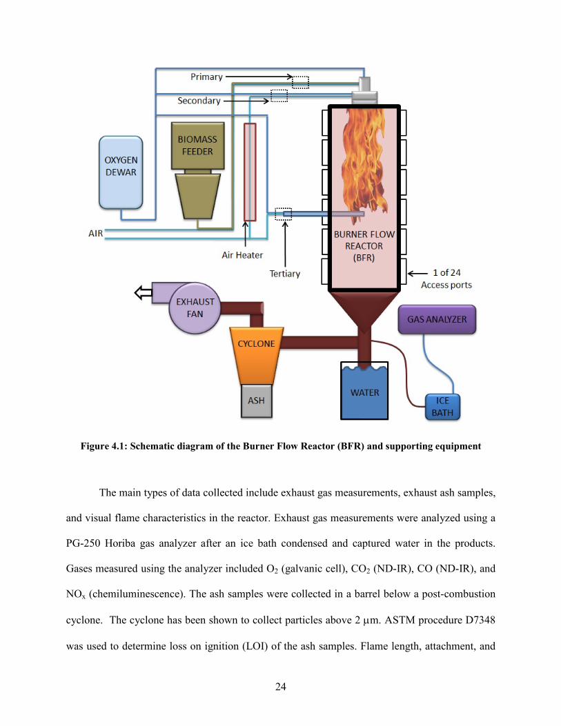
4.1 BYU Combustion Facility

The experiments were completed at the BYU oxy-combustion research facility shown

schematically in Figure 4.1. The fuel was burned in a 150 kWth down-fired Burner Flow Reactor

(BFR). The BFR is a cylindrical chamber with an inside diameter of 750 mm and length of

2.4 m, consisting of six vertical, 400 mm sections. Each of the sections has four access ports 90

degrees apart. The access ports are rectangular in shape with a height of 280 mm and width of 90

mm. The burner was mounted at the top and the fuel was down-fired. The reactor has a movable-

block, variable-swirl burner designed by Air Liquide.

The BFR is refractory lined on the inside and surrounded by water cooled walls. At the

base of the reactor there is a water barrel to catch deposits and to maintain positive pressure

within the reactor. Primary, secondary, and tertiary air lines are supplied by an Ingersol Rand

Compressor. A 265 liter liquid dewar supplies neat oxygen to the BFR in various locations using

the equipment as described and documented by Zeltner [43]. The fuel is fed to the reactor via a

bulk bag unloader and a gravimetric, computer-controlled, dual auger feeder.

24

Figure 4.1: Schematic diagram of the Burner Flow Reactor (BFR) and supporting equipment

The main types of data collected include exhaust gas measurements, exhaust ash samples,

and visual flame characteristics in the reactor. Exhaust gas measurements were analyzed using a

PG-250 Horiba gas analyzer after an ice bath condensed and captured water in the products.

Gases measured using the analyzer included O2 (galvanic cell), CO2 (ND-IR), CO (ND-IR), and

NOx (chemiluminescence). The ash samples were collected in a barrel below a post-combustion

cyclone. The cyclone has been shown to collect particles above 2 µm. ASTM procedure D7348

was used to determine loss on ignition (LOI) of the ash samples. Flame length, attachment, and

25

O2 flame characteristics were recorded from visual observation through glass windows on the

access ports of the reactor.

4.2 Fuel Analyses

Three types of biomass fuels, wheat straw, medium hardwood, and fine hardwood, were

used in this work. The proximate and ultimate analyses of the three types of fuel are displayed in

Table 4.1. The fuels have similar proximate and ultimate analyses with some difference in the

amount of ash and nitrogen. The straw has twice as much nitrogen content as the medium

hardwood (0.54% versus 0.26%) but neither has particularly high nitrogen content.

The ash content is much higher in the straw, 4.5%, compared to the wood, 0.3% and

0.54%. In addition to the larger ash fraction, ash from straw typically contains alkali which

lowers the melting temperature. This combined with the larger ash fraction causes a much larger

deposition rate for ash but the ash does not significantly impact combustion properties such as

flame length and flame stability. The fine wood is very similar to the medium wood, despite

being derived from different biomass stock.

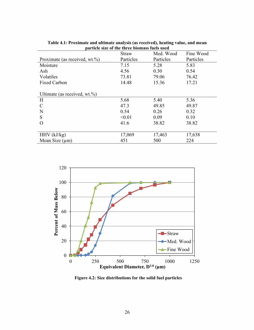
The three fuels also differ in particle size distribution as shown in Figure 4.2. Both the

straw and the medium wood have a similar mean particle size but the wood particles have a

much narrower size distribution meaning that the straw has both a greater number of larger and a

greater number of smaller particles. The straw may therefore be easier to ignite because of the

larger number of small particles but also more difficult to burn out because of the large particles.

Damstedt et al. [44] showed that straw contains particles called knees that are difficult to grind

and burn. The knees originate from the material between the hollow tube-like portions of the

straw. These knees are more dense and less volatile than the remainder of the straw particles.

26

Table 4.1: Proximate and ultimate analysis (as received), heating value, and mean particle size of the three biomass fuels used

Proximate (as received, wt.%) Straw Particles

Med. Wood Particles

Fine Wood Particles

Moisture 7.15 5.28 5.83 Ash 4.56 0.30 0.54 Volatiles 73.81 79.06 76.42 Fixed Carbon 14.48 15.36 17.21 Ultimate (as received, wt.%) H 5.68 5.40 5.36 C 47.3 49.85 49.87 N 0.54 0.26 0.32 S <0.01 0.09 0.10 O 41.6 38.82 38.82 HHV (kJ/kg) 17,069 17,463 17,638 Mean Size (µm) 451 500 224

0

20

40

60

80

100

120

0 250 500 750 1000 1250

Perc

ent o

f Mas

s Bel

ow

Equivalent Diameter, D3.0 (µm)

StrawMed. WoodFine Wood

Figure 4.2: Size distributions for the solid fuel particles

27

4.3 Burner Configurations and Operating Conditions

Below the variable block swirl chamber, the burner, designed by Air Liquide, utilized

three concentric tubes creating three flow channels. Multiple configurations were possible by

using tubes of various diameters. The tubes are numbered consecutively from the center outward

1-3, see Figure 4.3. For tube 1, three sizes are available: small, medium, and large. For tube 2,

two tubes: small and large. And for tube 3, two tubes: small and large. Abbreviations are used to

specify the burner configurations: for example 1S2L3L indicates the inner tube is small, the

second tube is large and the outer tube is large. The relative diameters of each tube in

comparison to the smallest diameter for tube 1 (19.05 mm) are shown in Table 4.2.

Figure 4.3 shows the cross section of the pipe in pipe burner showing locations of the

three concentric flows. Flow channel 1 represents the center tube of the burner through where

neat oxygen was typically injected. Flow channel 2 represents the annulus through which fuel

was entrained with the primary air. The flow rate of fuel was held constant at 29 kg/hr biomass.

This was selected to produce a nominal heating rate of 150 kWth which is sufficient to maintain

wall temperatures that will ignite and continuously burn fuel in the reactor. The primary air was

held constant at 14 kg/hr for both hardwood fuels and 20 kg/hr for straw unless otherwise

specified. In flow channel 3, secondary air was preheated to about 260 ℃ and held at a baseline

flow rate of 170 kg/hr for medium hardwood, 180 kg/hr for fine hardwood, and 158 kg/hr for

straw. The flow rate for primary air was selected by determining the lowest flow rate that would

consistently convey fuel from the feeder to the burner without plugging. The secondary air flow

was swirled using a variable swirl block prior to the burner exit. A ceramic quarl sits outside of

flow channel 3 that is shown in Figure 4.3 extends a relative length of 4.167 from the burner exit

and has dimensions as contained in Table 4.2.

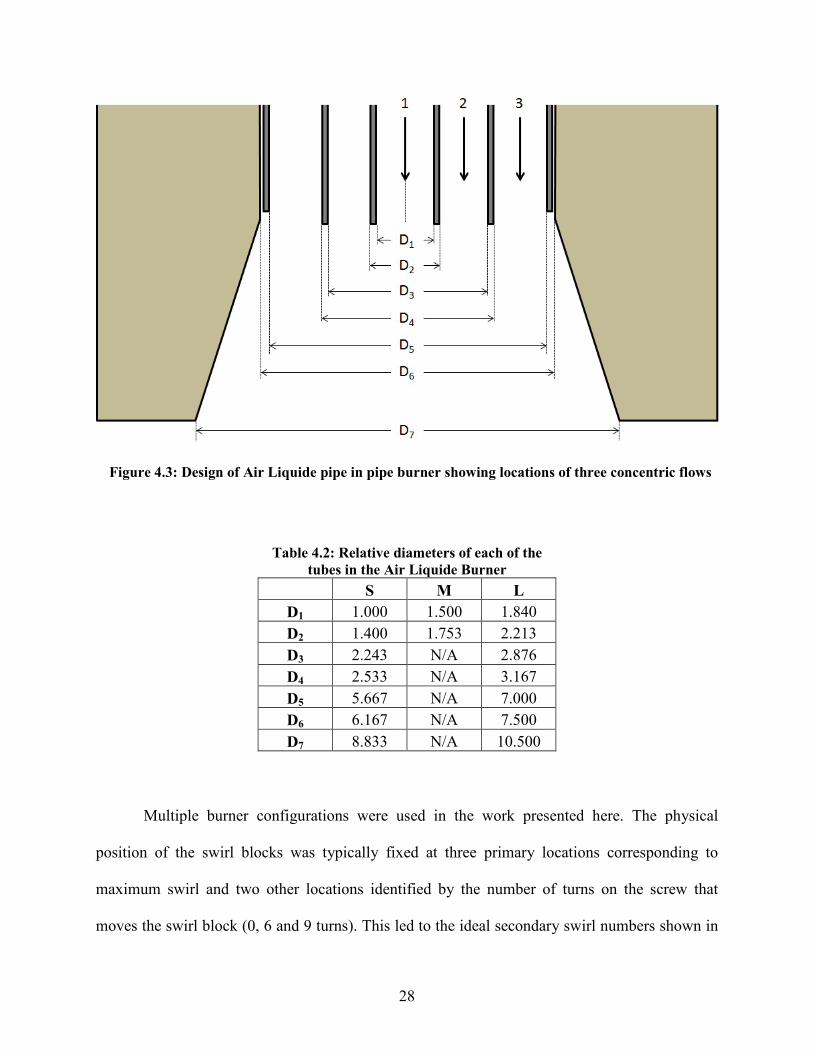
28

Table 4.2: Relative diameters of each of the tubes in the Air Liquide Burner

S M L

D1 1.000 1.500 1.840 D2 1.400 1.753 2.213 D3 2.243 N/A 2.876 D4 2.533 N/A 3.167 D5 5.667 N/A 7.000 D6 6.167 N/A 7.500 D7 8.833 N/A 10.500

Multiple burner configurations were used in the work presented here. The physical

position of the swirl blocks was typically fixed at three primary locations corresponding to

maximum swirl and two other locations identified by the number of turns on the screw that

moves the swirl block (0, 6 and 9 turns). This led to the ideal secondary swirl numbers shown in

Figure 4.3: Design of Air Liquide pipe in pipe burner showing locations of three concentric flows

29

Table 4.3 for the case where no oxygen was added. As oxygen was added to the center tube, the

swirl decreased slightly as there was no tangential component in the center flow, but increased

axial flow. Oxygen added to the secondary air negligibly increased the swirl.

Various operating conditions were completed for the selected number of configurations

used. For most of the conditions, oxygen varied from 0 – 8 kg/hr, in increments of 2 kg/hr. This

sweep of oxygen flow rates was completed for combinations of six burner configurations, three

oxygen locations, and the three fuels. The matrix of operating conditions for these configurations

is presented in Table 4.3.

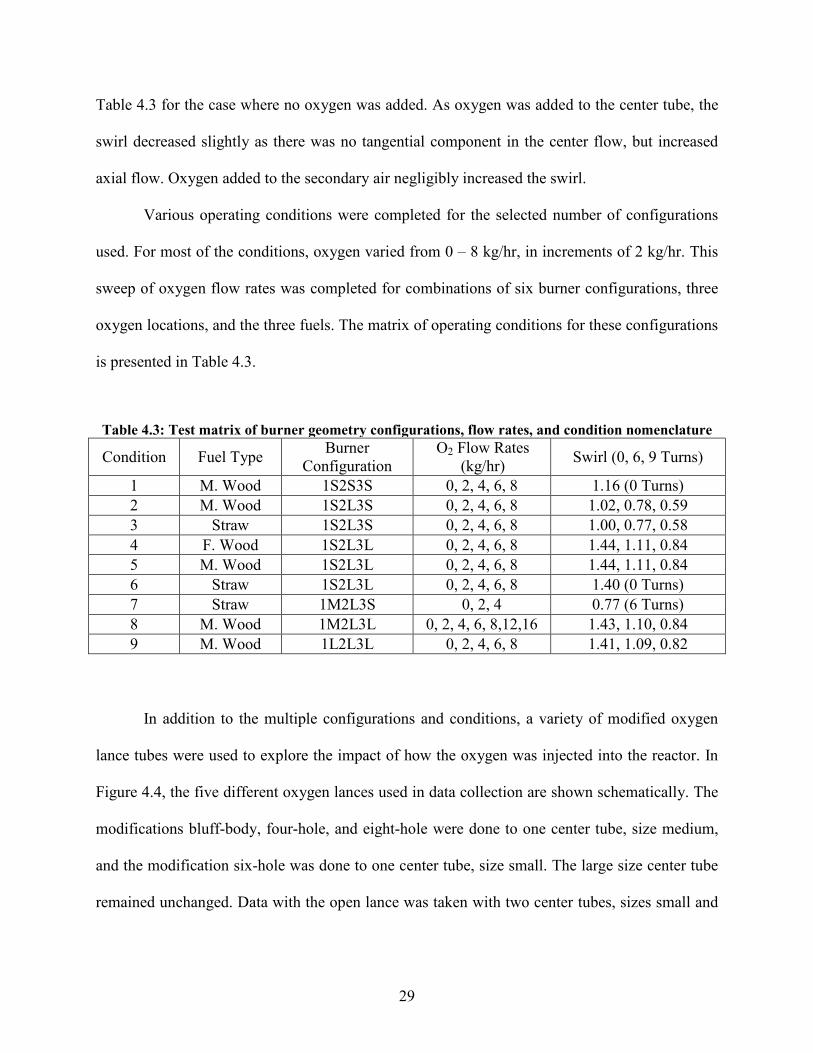
Table 4.3: Test matrix of burner geometry configurations, flow rates, and condition nomenclature

Condition Fuel Type Burner Configuration

O2 Flow Rates (kg/hr) Swirl (0, 6, 9 Turns)

1 M. Wood 1S2S3S 0, 2, 4, 6, 8 1.16 (0 Turns) 2 M. Wood 1S2L3S 0, 2, 4, 6, 8 1.02, 0.78, 0.59 3 Straw 1S2L3S 0, 2, 4, 6, 8 1.00, 0.77, 0.58 4 F. Wood 1S2L3L 0, 2, 4, 6, 8 1.44, 1.11, 0.84 5 M. Wood 1S2L3L 0, 2, 4, 6, 8 1.44, 1.11, 0.84 6 Straw 1S2L3L 0, 2, 4, 6, 8 1.40 (0 Turns) 7 Straw 1M2L3S 0, 2, 4 0.77 (6 Turns) 8 M. Wood 1M2L3L 0, 2, 4, 6, 8,12,16 1.43, 1.10, 0.84 9 M. Wood 1L2L3L 0, 2, 4, 6, 8 1.41, 1.09, 0.82

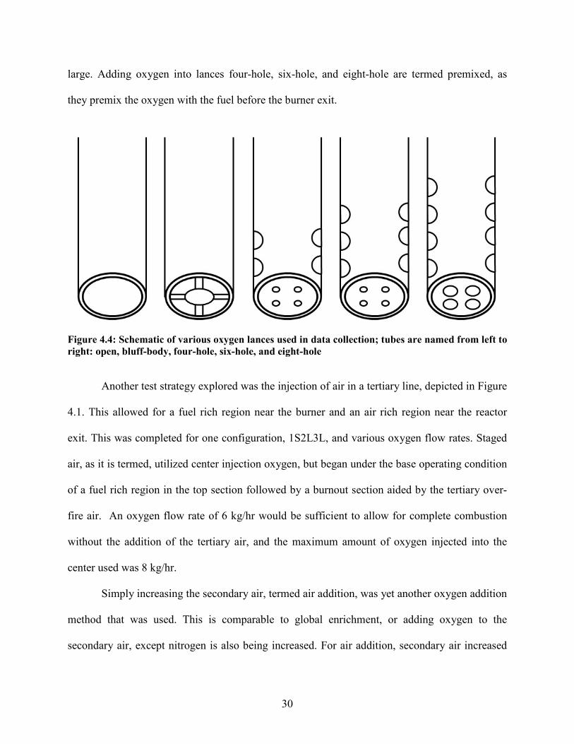
In addition to the multiple configurations and conditions, a variety of modified oxygen

lance tubes were used to explore the impact of how the oxygen was injected into the reactor. In

Figure 4.4, the five different oxygen lances used in data collection are shown schematically. The

modifications bluff-body, four-hole, and eight-hole were done to one center tube, size medium,

and the modification six-hole was done to one center tube, size small. The large size center tube

remained unchanged. Data with the open lance was taken with two center tubes, sizes small and

30

large. Adding oxygen into lances four-hole, six-hole, and eight-hole are termed premixed, as

they premix the oxygen with the fuel before the burner exit.

Another test strategy explored was the injection of air in a tertiary line, depicted in Figure

4.1. This allowed for a fuel rich region near the burner and an air rich region near the reactor

exit. This was completed for one configuration, 1S2L3L, and various oxygen flow rates. Staged

air, as it is termed, utilized center injection oxygen, but began under the base operating condition

of a fuel rich region in the top section followed by a burnout section aided by the tertiary over-

fire air. An oxygen flow rate of 6 kg/hr would be sufficient to allow for complete combustion

without the addition of the tertiary air, and the maximum amount of oxygen injected into the

center used was 8 kg/hr.

Simply increasing the secondary air, termed air addition, was yet another oxygen addition

method that was used. This is comparable to global enrichment, or adding oxygen to the

secondary air, except nitrogen is also being increased. For air addition, secondary air increased

Figure 4.4: Schematic of various oxygen lances used in data collection; tubes are named from left to right: open, bluff-body, four-hole, six-hole, and eight-hole

31

incrementally in amounts comparable to 2, 4, and 6 kg/hr of oxygen (roughly 9, 17, and 26 kg/hr

of air). Additional air was not added further due to the pressure of the supply line.

Lastly, the burner is capable of varying the exit location of the center tube relative to the

other tubes in the burner. The tube could be mounted flush, recessed, or extended beyond the exit

plane of the other two tubes. Multiple experiments were completed at various amounts of recess

and extension as well as a flush position with the burner exit.

4.4 NO Measurements

A continuous flow of the exhaust gas was sampled near the reactor exit as seen in Figure

4.1. The sample line first went through an ice bath to condense the water out of the exhaust line

and then continued to the gas analyzer. Upon entering the analyzer the gas passes through a

desiccant to produce a dry measurement. A PG-250 Horiba gas analyzer measured O2 (galvanic

cell), CO2 (ND-IR), CO (ND-IR), and NOx (chemiluminescence). Each of these gas species were

recorded three times at each operating condition during ash collection. The majority of this work

focuses on NO emission data collected and is reported herein. A calibration was completed in the

morning each day that data were collected. Changes in calibration from day to day were typically

less than 10%.

Two Rosemount Analytical ND-IR analyzers, for CO2 and CO, and a Beckman

chemiluminescence analyzer, for NOx, were used intermittently to verify the accuracy of the gas

measurements. A continuous zirconia based O2 sensor, like those used in automobile exhaust

lines was located near the gas sampling location. This sensor was used to monitor reactor

operation and provided a wet O2 concentration for comparison with the Horiba galvanic cell

measurement. After correcting for wet vs dry O2, the two sensors were normally in very good

32

agreement. Any differences between the two measurements were used to identify and correct

problems with the Horiba sample line.

4.5 Ash Collection and Loss on Ignition

Ash samples were collected in a barrel below the cyclone at the base of the reactor as

shown in Figure 4.1. Approximately 5 minutes after changing an operating condition, gases

measured became steady. At this point, an ash sample was initiated. To begin ash sampling, a

thin metal plate was cleaned and placed in the bottom of the cyclone barrel. The barrel was also

cleaned with a jet of air before each sample. Once sufficient time passed for the ash to collect in

the barrel, roughly 5 to 10 minutes, the metal plate was removed and the ash was placed in a

small vial. Finally, the ash samples were placed in crucibles for loss on ignition (LOI)

measurement.

LOI is a measure of the mass fraction removed from a dried sample when heated to a

temperature high enough to oxidize the non-inert material. Typically, the mass removed is

almost entirely carbon and therefore LOI can be used to approximate carbon burnout. ASTM

procedure D7348 was normally used to determine LOI for the ash samples. This procedure

involves first heating the particles to 105℃ for 4 hours to remove the moisture. The weight of the

moisture free ash, 𝑊𝑚𝑚𝑚, is then measured. The ash is then heated to 950℃ for 6-8 hours and

weighed to produce the weight of the carbon free ash, 𝑊𝑐𝑚𝑚. The two weights are then used to

calculate the LOI and carbon burnout as shown in Equations 4.1 and 4.2. 𝑌𝑚𝑎ℎ is the ash content

as determined from the proximate analysis of the fuel. This procedure was repeated three times

for each sample and the average of those three measurements is reported as the LOI value for

that sample.

33

𝐿𝑂𝐿 = 𝑊𝑚𝑚𝑚 − 𝑊𝑐𝑚𝑚

𝑊𝑚𝑚𝑚 (4.1)

𝐶𝐶𝐶𝐶𝐶𝐶 𝐵𝐵𝐶𝐶𝐶𝐵𝐵 % = 1 − 𝑌𝑚𝑎ℎ − 𝐿𝑂𝐿

(1 − 𝐿𝑂𝐿) ∗ (1 − 𝑌𝑚𝑎ℎ) (4.2)

This procedure was found to be problematic for the straw ash. The straw ash melted and

sintered together at 950℃ making complete oxidation of the carbon difficult as it became trapped

beneath molten slag. The oxidation temperature was lowered from 950℃ to 750℃ for the straw

ash to allow the carbon particles to be consumed without sintering. Tests were then completed to

verify the effectiveness of the adjusted method. Samples were removed and weighed after

various time periods at 750℃ until the weight reached a minimum and was no longer changing.

It was determined that a longer period of time, 10-12 hours, at the lower temperature is needed to

ensure complete burnout. Results at the lower temperature on wood ash were also compared to

results at the higher temperature to ensure all of the carbon was being oxidized. At a temperature

of 750℃ the wood ash resulted in nominally the same LOI as was found at 950℃, see Table 4.4.

The table reveals that the higher temperature for the straw was ineffective at producing the total

LOI as the mass sintered before the carbon was entirely consumed. Data confirmed that the

lower temperature of 750℃ was high enough to complete carbon oxidation.

Table 4.4: LOI measurements from two different fuels and temperatures

Sample LOI at 950oC

LOI at 750oC Difference

M. Wood 1 38.21 % 38.61 % -1.05 % M. Wood 2 29.28 % 29.10 % 0.59 % M. Wood 3 23.04 % 22.93 % 0.47 % M. Wood 4 18.45 % 18.59 % -0.78 %

Straw 1 25.55 % 20.61 % 19.36 % Straw 2 18.05 % 14.50 % 19.68 % Straw 3 16.27 % 11.09 % 31.85 % Straw 4 9.97 % 6.51 % 34.69 %

35

5 NO AND LOI RESULTS AND DISCUSSION

Experimental results presented in this chapter include measurements of NO exhaust gas

and LOI. Relationships between various operating conditions are presented. Following the

presentation of the data, the results will be summarized and discussed.

5.1 Nitric Oxide Emission (NO)

The following data present the impact of swirl, oxygen flow rate, oxygen injection

location, and burner configuration on NO in the exhaust. All of the results shown in this section

are for medium hardwood biomass. The reported NO measurements are an average of three

recorded values at each operating condition during simultaneous ash collection.

5.1.1 NO vs. Swirl

The effect of swirl and oxygen flow rate on exhaust NO, for a burner configuration of

1S2L3L, can been seen in Figure 5.1. Solid lines connect points of equal oxygen flow rate and

variable swirl. Figure 5.1a shows data where the oxygen is added to the secondary line (global

enrichment) and Figure 5.1b shows data with oxygen being injected through the center via a

lance that is in a recessed position of 76 mm from the burner exit plane. For all cases the

secondary air flow rate was held constant.

36

The exhaust NO concentration is seen to increase with an increase in swirl and with an

increase in O2 flow rate. While the increase in NO is relatively linear with increasing swirl, the

increase in NO is non-linear with increasing O2 center injection.

(a) Global Enrichment

(b) Center Injection

Error bars located on this plot were determined by an uncertainty analysis provided in

Appendix B.1. Precision error for NO was determined to be negligible compared to instrument

bias and measurement repeatability. To reduce bias error, the exhaust analyzer was calibrated

prior to each day of measurement collection. The most significant source of error was found to

be process repeatability. The repeatability was determined by comparing results from 12 data

sets where the same operating conditions were repeated at least once. The standard deviation for

each of these twelve data sets was calculated and multiplied by two. The standard deviation was

then divided by the average to obtain the uncertainty for each of the twelve repeated data sets

and this uncertainty was averaged to obtain the results in Table 5.1; ± 5.58% for NO and ±

0

50

100

150

200

0.50 0.75 1.00 1.25 1.50

NO

(ppm

)

Swirl

O2 - 0 kg/hrO2 - 2 kg/hrO2 - 4 kg/hrO2 - 6 kg/hrO2 - 8 kg/hr

0

50

100

150

200

0.50 0.75 1.00 1.25 1.50N

O (p

pm)

Swirl


Figure 5.1: NO (ppm) vs. Swirl at varying oxygen flow rates, configuration 1S2L3L, medium hardwood, constant secondary air for (a) Global Enrichment and (b) Center Injection

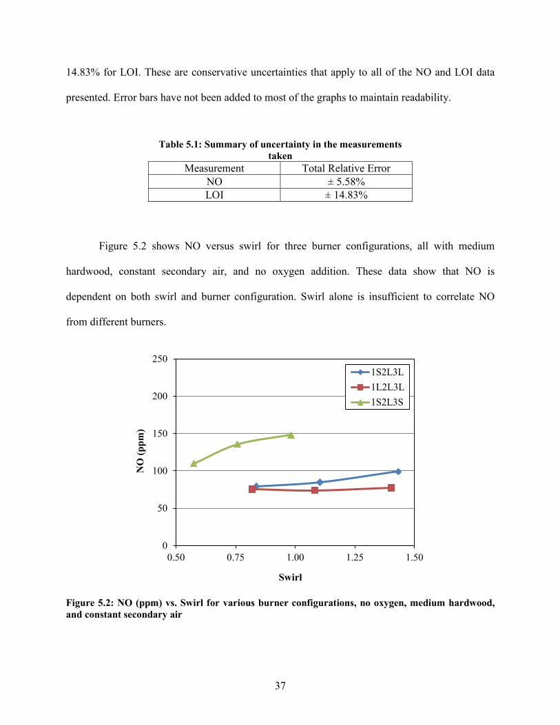
37

14.83% for LOI. These are conservative uncertainties that apply to all of the NO and LOI data

presented. Error bars have not been added to most of the graphs to maintain readability.

Table 5.1: Summary of uncertainty in the measurements taken

Measurement Total Relative Error NO ± 5.58% LOI ± 14.83%

Figure 5.2 shows NO versus swirl for three burner configurations, all with medium

hardwood, constant secondary air, and no oxygen addition. These data show that NO is

dependent on both swirl and burner configuration. Swirl alone is insufficient to correlate NO

from different burners.

0

50

100

150

200

250

0.50 0.75 1.00 1.25 1.50

NO

(ppm

)

Swirl

1S2L3L1L2L3L1S2L3S

Figure 5.2: NO (ppm) vs. Swirl for various burner configurations, no oxygen, medium hardwood, and constant secondary air

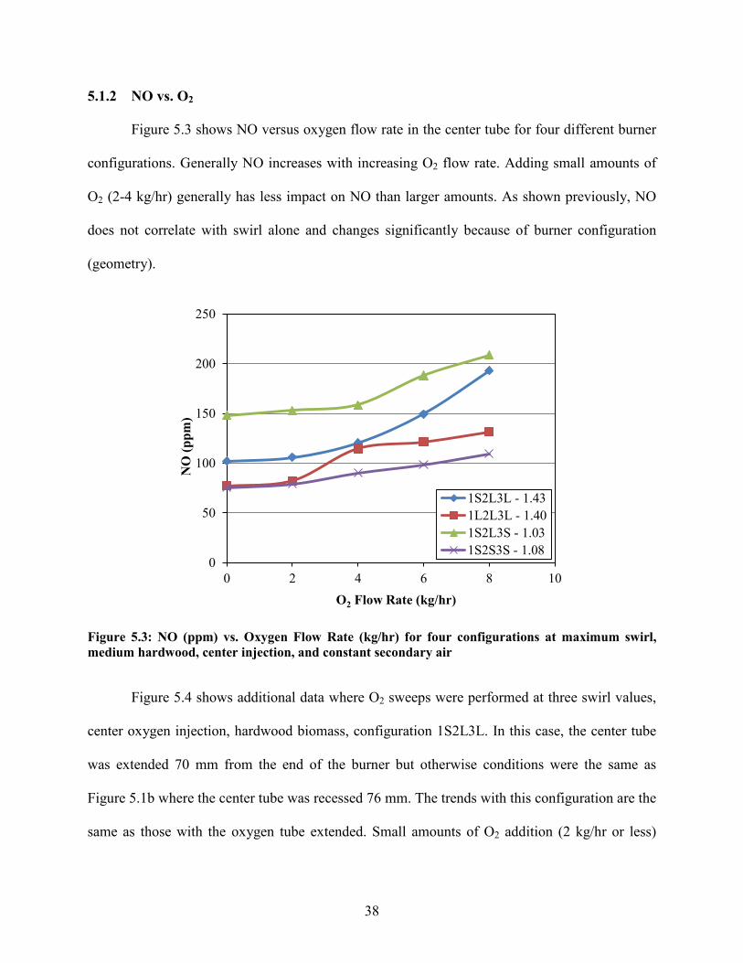
38

5.1.2 NO vs. O2

Figure 5.3 shows NO versus oxygen flow rate in the center tube for four different burner

configurations. Generally NO increases with increasing O2 flow rate. Adding small amounts of

O2 (2-4 kg/hr) generally has less impact on NO than larger amounts. As shown previously, NO

does not correlate with swirl alone and changes significantly because of burner configuration

(geometry).

Figure 5.4 shows additional data where O2 sweeps were performed at three swirl values,

center oxygen injection, hardwood biomass, configuration 1S2L3L. In this case, the center tube

was extended 70 mm from the end of the burner but otherwise conditions were the same as

Figure 5.1b where the center tube was recessed 76 mm. The trends with this configuration are the

same as those with the oxygen tube extended. Small amounts of O2 addition (2 kg/hr or less)

0

50

100

150

200

250

0 2 4 6 8 10

NO

(ppm

)

O2 Flow Rate (kg/hr)

1S2L3L - 1.431L2L3L - 1.401S2L3S - 1.031S2S3S - 1.08

Figure 5.3: NO (ppm) vs. Oxygen Flow Rate (kg/hr) for four configurations at maximum swirl, medium hardwood, center injection, and constant secondary air

39

produced only small increases of NO. With higher flow rates of oxygen in the center tube, NO

emissions increased more significantly.

5.1.3 NO vs. Primary Air

Figure 5.5 shows NO as a function of primary air flow rate for configuration 1S2L3L. In

one case, the center tube is recessed 76 mm and in the other case, the center tube is flush with the

end of the burner and utilizes the six-hole lance as shown in Figure 4.4. In both of the data sets

shown, there is no oxygen introduced into the reactor. The data show that an increase in primary

flow decreases NO and that the center tube recessed produces more NO than a flush center tube.

0

50

100

150

200

250

0 2 4 6 8 10

NO

(ppm

)


Swirl - 1.43Swirl - 1.10Swirl - 0.84

Figure 5.4: NO (ppm) vs. Oxygen Flow Rate (kg/hr) and varying swirl for the medium hardwood, configuration 1S2L3L, center injection, tube 1 extended 70 mm

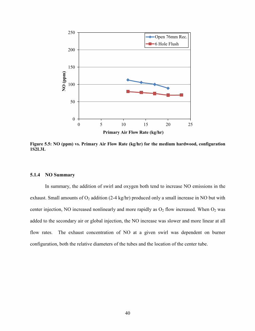
40

Figure 5.5: NO (ppm) vs. Primary Air Flow Rate (kg/hr) for the medium hardwood, configuration 1S2L3L

5.1.4 NO Summary

In summary, the addition of swirl and oxygen both tend to increase NO emissions in the

exhaust. Small amounts of O2 addition (2-4 kg/hr) produced only a small increase in NO but with

center injection, NO increased nonlinearly and more rapidly as O2 flow increased. When O2 was

added to the secondary air or global injection, the NO increase was slower and more linear at all

flow rates. The exhaust concentration of NO at a given swirl was dependent on burner

configuration, both the relative diameters of the tubes and the location of the center tube.

0

50

100

150

200

250

0 5 10 15 20 25

NO

(ppm

)

Primary Air Flow Rate (kg/hr)

Open 76mm Rec.6 Hole Flush

41

5.2 Loss on Ignition (LOI)

This section shows the impact of swirl, oxygen flow rate, oxygen injection location, and

burner configuration on LOI. The LOI values reported are an average of three measurements

from a single ash sample.

5.2.1 LOI vs. Swirl

The effect of swirl and oxygen flow rate on LOI, for a burner configuration of 1S2L3L,

can be seen in Figure 5.6. Figure 5.6a shows data where the oxygen is added to the secondary

line (global enrichment), and Figure 5.6b is for center injection. The trends for LOI are opposite

in comparison to NO. As swirl increases, LOI decreases. In these figures, the secondary flow rate

is held constant effectively increasing the oxygen concentration in the exhaust. As the oxygen

flow rate increases the LOI decreases. The LOI values for both global enrichment and center

injection are comparable for most oxygen flow rates and swirl values.



0%

10%

20%

30%

40%

50%

60%

0.00 0.40 0.80 1.20 1.60

LO

I

Swirl


0%

10%

20%

30%

40%

50%

60%

0.00 0.40 0.80 1.20 1.60

LO

I

Swirl


Figure 5.6: LOI vs. Swirl at five flow rates of oxygen in the center, configuration 1S2L3L, medium hardwood, and constant secondary air for (a) Global Enrichment and (b) Center Injection

42

Error bars on this plot were determined by an uncertainty analysis and explained in the

Appendix B.1. See Table 5.1 for a summary of the uncertainty values. These errors bars are

estimated to be the error associated with all collected LOI data herein. Most of the remaining

plots are shown without error bars.

Figure 5.7 shows LOI versus swirl for three burner configurations, same as those shown

in Figure 5.2. These data show that LOI has a dependence on both swirl and burner

configuration. Swirl alone cannot be used to correlate LOI from various burners.

5.2.2 LOI vs. O2

Figure 5.8 shows LOI versus oxygen flow rate in the center tube for four different

configurations. LOI decreases with increasing amounts of oxygen. Initially the rate at which LOI

decreases can be rapid with small amounts of oxygen (0-4 kg/hr), but then slows at the higher

flow rates (6-8 hg/hr).

0%

10%

20%

30%

40%

50%

60%

0.50 0.75 1.00 1.25 1.50

LO

I

Swirl

1S2L3L1L2L3L1S2L3S

Figure 5.7: LOI vs. Swirl for various burner configurations, no oxygen, medium hardwood, and constant secondary air

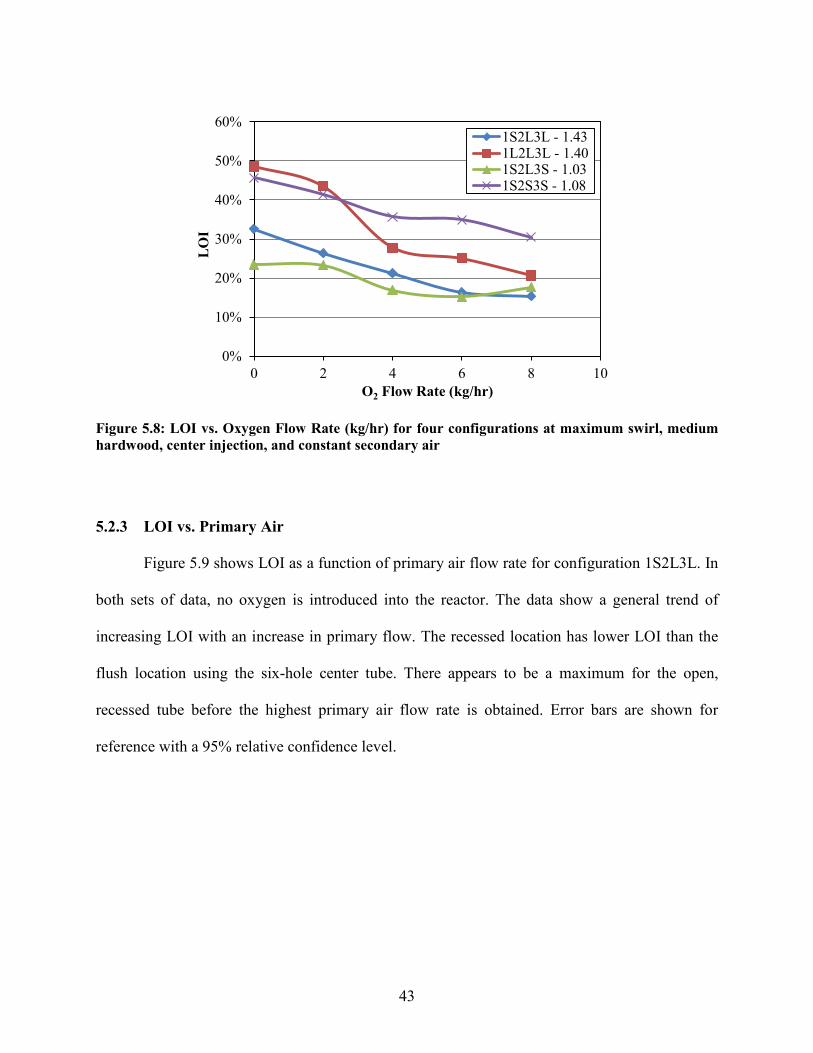
43

5.2.3 LOI vs. Primary Air

Figure 5.9 shows LOI as a function of primary air flow rate for configuration 1S2L3L. In

both sets of data, no oxygen is introduced into the reactor. The data show a general trend of

increasing LOI with an increase in primary flow. The recessed location has lower LOI than the

flush location using the six-hole center tube. There appears to be a maximum for the open,

recessed tube before the highest primary air flow rate is obtained. Error bars are shown for

reference with a 95% relative confidence level.

0%

10%

20%

30%

40%

50%

60%

0 2 4 6 8 10

LO

I


1S2L3L - 1.431L2L3L - 1.401S2L3S - 1.031S2S3S - 1.08

Figure 5.8: LOI vs. Oxygen Flow Rate (kg/hr) for four configurations at maximum swirl, medium hardwood, center injection, and constant secondary air

44

Figure 5.9: LOI vs. Primary Air Flow Rate (kg/hr) for the medium hardwood, configuration 1S2L3L

5.2.4 LOI Summary

LOI was found to decrease with increasing swirl and oxygen concentration. The amount

of LOI reduction for a given increase in O2 was often lower at high O2 flow rates showing a

reduced benefit to O2 addition. LOI did not correlate with swirl for all burner configurations.

Recessing the primary tube or reducing the primary air flow rate had a tendency to decrease LOI.

5.3 NO vs. LOI Trade-off

Given the observation that changes in operating conditions or burner configurations

typically produce opposite trends for NO and LOI, decreasing one while increasing the other it is

advantageous to analyze the impacts of variable on both exhaust products at the same time. As a

result, NO and LOI have been plotted on the same graph producing NO – LOI trade-off curves.

This section presents these curves and utilizes them to discuss the results.

0%

10%

20%

30%

40%

50%

60%

0 5 10 15 20 25

LO

I

Primary Air Flow Rate (kg/hr)


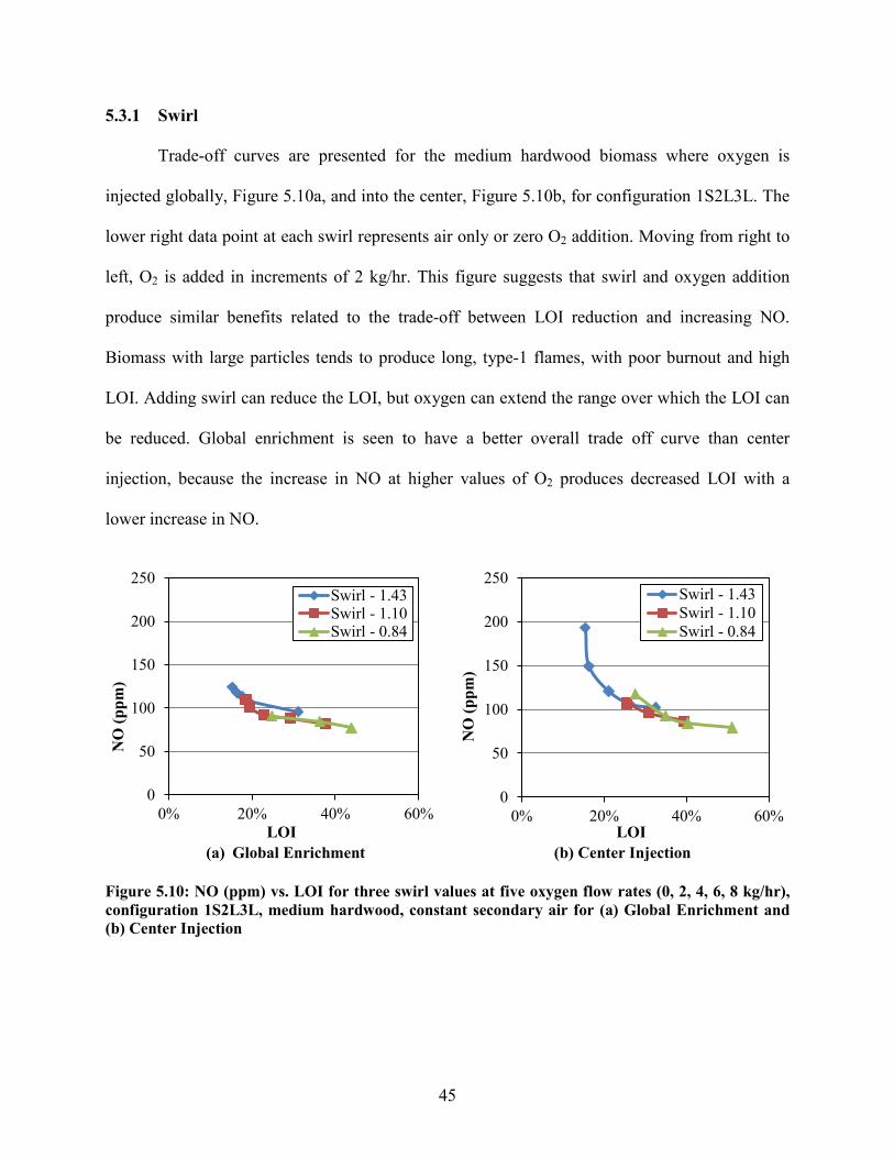
45

5.3.1 Swirl

Trade-off curves are presented for the medium hardwood biomass where oxygen is

injected globally, Figure 5.10a, and into the center, Figure 5.10b, for configuration 1S2L3L. The

lower right data point at each swirl represents air only or zero O2 addition. Moving from right to

left, O2 is added in increments of 2 kg/hr. This figure suggests that swirl and oxygen addition

produce similar benefits related to the trade-off between LOI reduction and increasing NO.

Biomass with large particles tends to produce long, type-1 flames, with poor burnout and high

LOI. Adding swirl can reduce the LOI, but oxygen can extend the range over which the LOI can

be reduced. Global enrichment is seen to have a better overall trade off curve than center

injection, because the increase in NO at higher values of O2 produces decreased LOI with a

lower increase in NO.



0

50

100

150

200

250

0% 20% 40% 60%

NO

(ppm

)

LOI


0

50

100

150

200

250

0% 20% 40% 60%

NO

(ppm

)

LOI


Figure 5.10: NO (ppm) vs. LOI for three swirl values at five oxygen flow rates (0, 2, 4, 6, 8 kg/hr), configuration 1S2L3L, medium hardwood, constant secondary air for (a) Global Enrichment and (b) Center Injection

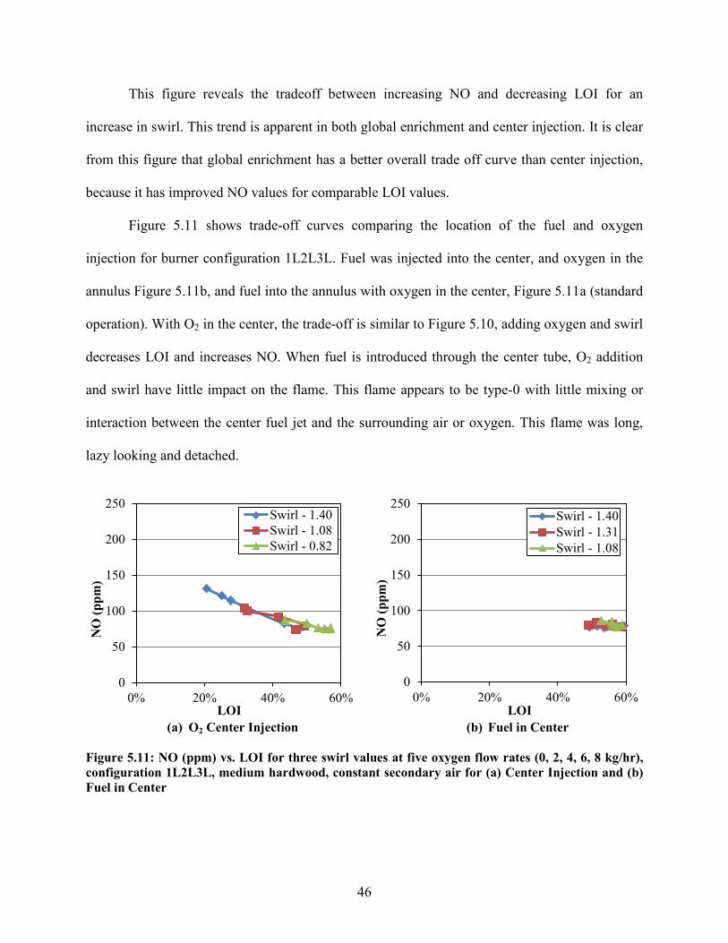
46

This figure reveals the tradeoff between increasing NO and decreasing LOI for an

increase in swirl. This trend is apparent in both global enrichment and center injection. It is clear

from this figure that global enrichment has a better overall trade off curve than center injection,

because it has improved NO values for comparable LOI values.

Figure 5.11 shows trade-off curves comparing the location of the fuel and oxygen

injection for burner configuration 1L2L3L. Fuel was injected into the center, and oxygen in the

annulus Figure 5.11b, and fuel into the annulus with oxygen in the center, Figure 5.11a (standard

operation). With O2 in the center, the trade-off is similar to Figure 5.10, adding oxygen and swirl

decreases LOI and increases NO. When fuel is introduced through the center tube, O2 addition

and swirl have little impact on the flame. This flame appears to be type-0 with little mixing or

interaction between the center fuel jet and the surrounding air or oxygen. This flame was long,

lazy looking and detached.

(a) O2 Center Injection

(b) Fuel in Center

0

50

100

150

200

250

0% 20% 40% 60%

NO

(ppm

)

LOI


0

50

100

150

200

250

0% 20% 40% 60%

NO

(ppm

)

LOI


Figure 5.11: NO (ppm) vs. LOI for three swirl values at five oxygen flow rates (0, 2, 4, 6, 8 kg/hr), configuration 1L2L3L, medium hardwood, constant secondary air for (a) Center Injection and (b) Fuel in Center

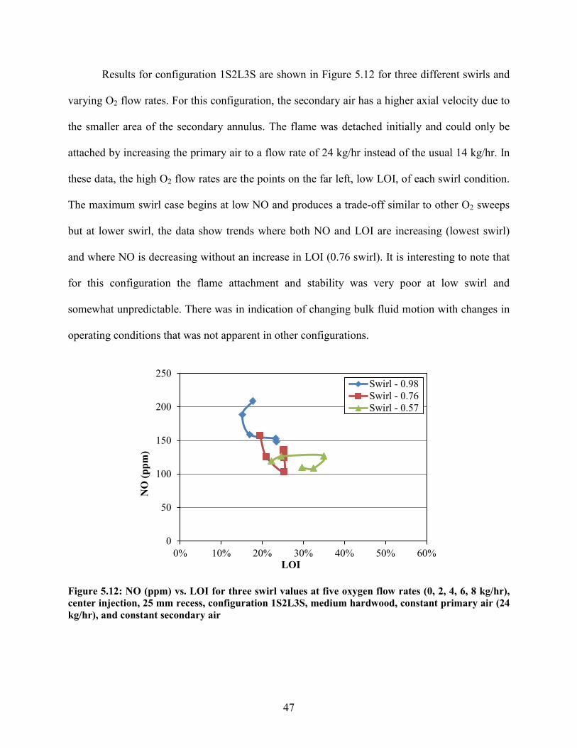
47

Results for configuration 1S2L3S are shown in Figure 5.12 for three different swirls and

varying O2 flow rates. For this configuration, the secondary air has a higher axial velocity due to

the smaller area of the secondary annulus. The flame was detached initially and could only be

attached by increasing the primary air to a flow rate of 24 kg/hr instead of the usual 14 kg/hr. In

these data, the high O2 flow rates are the points on the far left, low LOI, of each swirl condition.

The maximum swirl case begins at low NO and produces a trade-off similar to other O2 sweeps

but at lower swirl, the data show trends where both NO and LOI are increasing (lowest swirl)

and where NO is decreasing without an increase in LOI (0.76 swirl). It is interesting to note that

for this configuration the flame attachment and stability was very poor at low swirl and

somewhat unpredictable. There was in indication of changing bulk fluid motion with changes in

operating conditions that was not apparent in other configurations.

0

50

100

150

200

250

0% 10% 20% 30% 40% 50% 60%

NO

(ppm

)

LOI


Figure 5.12: NO (ppm) vs. LOI for three swirl values at five oxygen flow rates (0, 2, 4, 6, 8 kg/hr), center injection, 25 mm recess, configuration 1S2L3S, medium hardwood, constant primary air (24 kg/hr), and constant secondary air

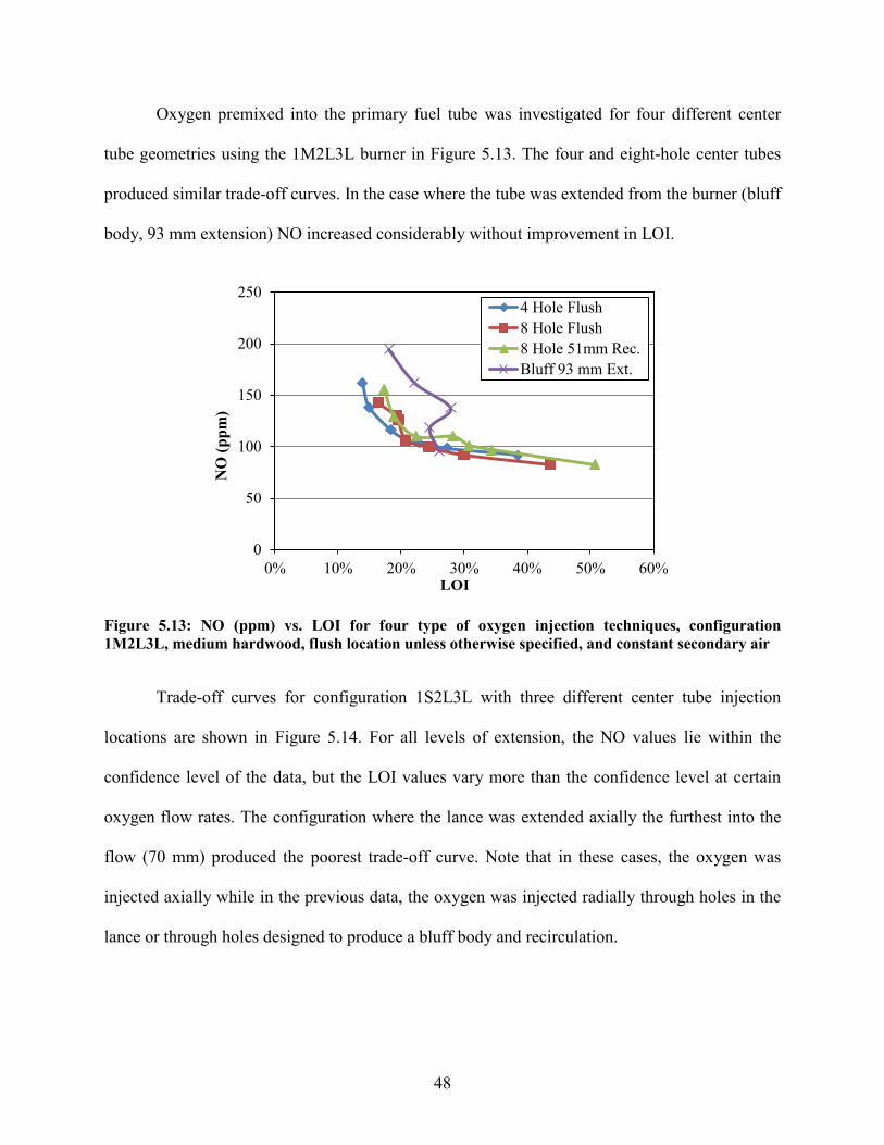
48

Oxygen premixed into the primary fuel tube was investigated for four different center

tube geometries using the 1M2L3L burner in Figure 5.13. The four and eight-hole center tubes

produced similar trade-off curves. In the case where the tube was extended from the burner (bluff

body, 93 mm extension) NO increased considerably without improvement in LOI.

Trade-off curves for configuration 1S2L3L with three different center tube injection

locations are shown in Figure 5.14. For all levels of extension, the NO values lie within the

confidence level of the data, but the LOI values vary more than the confidence level at certain

oxygen flow rates. The configuration where the lance was extended axially the furthest into the

flow (70 mm) produced the poorest trade-off curve. Note that in these cases, the oxygen was

injected axially while in the previous data, the oxygen was injected radially through holes in the

lance or through holes designed to produce a bluff body and recirculation.

0

50

100

150

200

250

0% 10% 20% 30% 40% 50% 60%

NO

(ppm

)

LOI

4 Hole Flush8 Hole Flush8 Hole 51mm Rec.Bluff 93 mm Ext.

Figure 5.13: NO (ppm) vs. LOI for four type of oxygen injection techniques, configuration 1M2L3L, medium hardwood, flush location unless otherwise specified, and constant secondary air

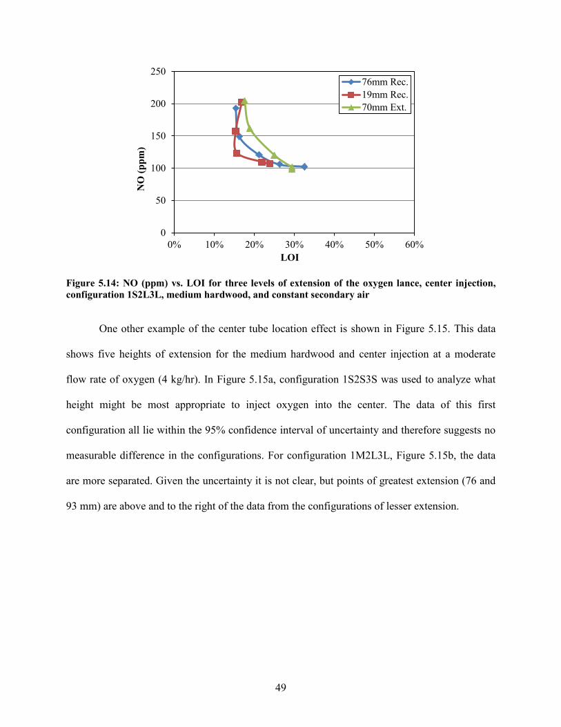
49

One other example of the center tube location effect is shown in Figure 5.15. This data

shows five heights of extension for the medium hardwood and center injection at a moderate

flow rate of oxygen (4 kg/hr). In Figure 5.15a, configuration 1S2S3S was used to analyze what

height might be most appropriate to inject oxygen into the center. The data of this first

configuration all lie within the 95% confidence interval of uncertainty and therefore suggests no

measurable difference in the configurations. For configuration 1M2L3L, Figure 5.15b, the data

are more separated. Given the uncertainty it is not clear, but points of greatest extension (76 and

93 mm) are above and to the right of the data from the configurations of lesser extension.

0

50

100

150

200

250

0% 10% 20% 30% 40% 50% 60%

NO

(ppm

)

LOI

76mm Rec.19mm Rec.70mm Ext.

Figure 5.14: NO (ppm) vs. LOI for three levels of extension of the oxygen lance, center injection, configuration 1S2L3L, medium hardwood, and constant secondary air

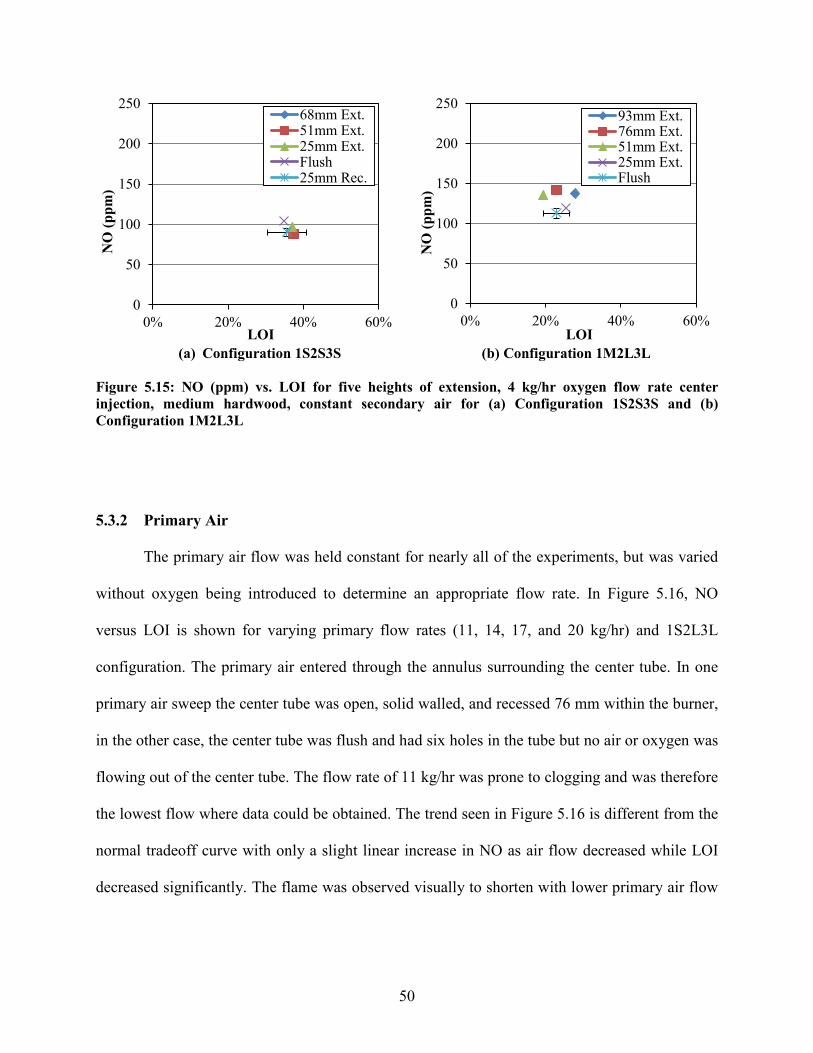
50

(a) Configuration 1S2S3S

(b) Configuration 1M2L3L

5.3.2 Primary Air

The primary air flow was held constant for nearly all of the experiments, but was varied

without oxygen being introduced to determine an appropriate flow rate. In Figure 5.16, NO

versus LOI is shown for varying primary flow rates (11, 14, 17, and 20 kg/hr) and 1S2L3L

configuration. The primary air entered through the annulus surrounding the center tube. In one

primary air sweep the center tube was open, solid walled, and recessed 76 mm within the burner,

in the other case, the center tube was flush and had six holes in the tube but no air or oxygen was

flowing out of the center tube. The flow rate of 11 kg/hr was prone to clogging and was therefore

the lowest flow where data could be obtained. The trend seen in Figure 5.16 is different from the

normal tradeoff curve with only a slight linear increase in NO as air flow decreased while LOI

decreased significantly. The flame was observed visually to shorten with lower primary air flow

0

50

100

150

200

250

0% 20% 40% 60%

NO

(ppm

)

LOI

68mm Ext.51mm Ext.25mm Ext.Flush25mm Rec.

0

50

100

150

200

250

0% 20% 40% 60%

NO

(ppm

)

LOI

93mm Ext.76mm Ext.51mm Ext.25mm Ext.Flush

Figure 5.15: NO (ppm) vs. LOI for five heights of extension, 4 kg/hr oxygen flow rate center injection, medium hardwood, constant secondary air for (a) Configuration 1S2S3S and (b) Configuration 1M2L3L

51

rates. The decrease in primary air is likely to cause a shift from a type 1 flame toward a type 2

flame allowing more entrainment of particles.

Data with the six-hole center tube can also be seen in Figure 5.16, with a very different

starting location. In this data set primary air flow rates of 11, 14, 17, 20, and 23 were attempted.

Once again the trend was identical, albeit shifted, and led to the same conclusions as before, to

use a low primary flow rate that successfully carries the fuel.

Data were collected at three oxygen flow rates (0, 4, and 8 kg/hr) using configuration

1S2L3L and the premix six-hole oxygen lance. This data is shown in Figure 5.17 at two primary

flow rates, 11 and 14 kg/hr. In these data there is no measureable difference.

0

50

100

150

200

250

0% 10% 20% 30% 40% 50% 60%

NO

(ppm

)

LOI


Figure 5.16: NO (ppm) vs. LOI for varying primary flow rates, no oxygen introduced, medium hardwood, configuration 1S2L3L

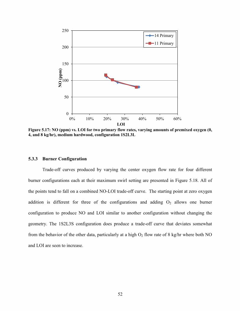
52

5.3.3 Burner Configuration

Trade-off curves produced by varying the center oxygen flow rate for four different

burner configurations each at their maximum swirl setting are presented in Figure 5.18. All of

the points tend to fall on a combined NO-LOI trade-off curve. The starting point at zero oxygen

addition is different for three of the configurations and adding O2 allows one burner

configuration to produce NO and LOI similar to another configuration without changing the

geometry. The 1S2L3S configuration does produce a trade-off curve that deviates somewhat

from the behavior of the other data, particularly at a high O2 flow rate of 8 kg/hr where both NO

and LOI are seen to increase.

0

50

100

150

200

250

0% 10% 20% 30% 40% 50% 60%

NO

(ppm

)

LOI

14 Primary

11 Primary

Figure 5.17: NO (ppm) vs. LOI for two primary flow rates, varying amounts of premixed oxygen (0, 4, and 8 kg/hr), medium hardwood, configuration 1S2L3L

53

5.3.4 Variable vs. Constant Secondary Flow Rate

For most of the data, the addition of oxygen means a greater overall flow of oxygen

through the reactor and a greater exit concentration of O2. In addition to this typical case, data

were collected where the secondary air flow rate was decreased as oxygen was injected in order

to keep the overall O2 flow rate constant and the exit concentration of O2 constant at nominally

3%. In the data in Figure 5.19, the secondary flow rate is varied such that the oxygen

concentration in the exhaust is held roughly constant. The total nitrogen in the reactor is

therefore effectively decreased with increasing oxygen amounts. Shown in this figure are where

oxygen is injected globally, Figure 5.19a, and into the center, Figure 5.19b. Beginning with

Figure 5.19a, 0 kg/hr of oxygen has the lowest LOI for each swirl value. Upon adding O2, LOI

increases with slight but varied responses of NO. The increase of LOI with additional O2 is

opposite of previous trends seen. Increasing the swirl seems to make higher NO, but with

moderate improvements to LOI. For 0 kg/hr of center injection, Figure 5.19b, NO values are low.

0

50

100

150

200

250

0% 10% 20% 30% 40% 50% 60%

NO

(ppm

)

LOI

1S2L3L - 1.431L2L3L - 1.401S2L3S - 1.031S2S3S - 1.08

Figure 5.18: NO (ppm) vs. LOI at maximum swirl for four different configurations, varying amounts of oxygen flow rates, center injection, medium hardwood, and constant secondary air

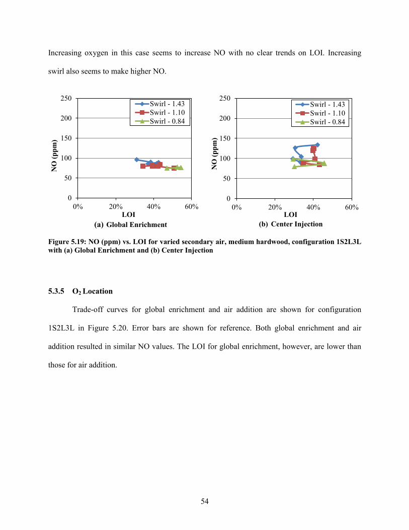
54

Increasing oxygen in this case seems to increase NO with no clear trends on LOI. Increasing

swirl also seems to make higher NO.



5.3.5 O2 Location

Trade-off curves for global enrichment and air addition are shown for configuration

1S2L3L in Figure 5.20. Error bars are shown for reference. Both global enrichment and air

addition resulted in similar NO values. The LOI for global enrichment, however, are lower than

those for air addition.

0

50

100

150

200

250

0% 20% 40% 60%

NO

(ppm

)

LOI


0

50

100

150

200

250

0% 20% 40% 60%N

O (p

pm)

LOI


Figure 5.19: NO (ppm) vs. LOI for varied secondary air, medium hardwood, configuration 1S2L3L with (a) Global Enrichment and (b) Center Injection

55

Trade-off curves for sweeps of O2 for the five main oxygen injection techniques used in

this work, over-fire air, premixed oxygen, center injection, global enrichment, and air addition,

are shown for configuration 1S2L3L in Figure 5.21. Curves closer to the origin are considered

better than those further from the origin because of the overall lower exhaust product values.

Using center injection as the base case, each of the other four oxygen addition techniques

resulted in an improved result. Global enrichment, air addition, and premixed oxygen resulted in

very similar tradeoff curves, but global O2 addition was able to achieve lower LOI values. Over-

fire air produced a trade-off between global and center O2 injection. Air addition matched the

NO values that were obtained with global enrichment, but with worse LOI values.

80

100

120

140

160

10% 15% 20% 25% 30% 35%

NO

(ppm

)

LOI

GlobalAir Addition

Figure 5.20: NO (ppm) vs. LOI for two oxygen addition techniques, global enrichment and air addition, configuration 1S2L3L, and medium hardwood

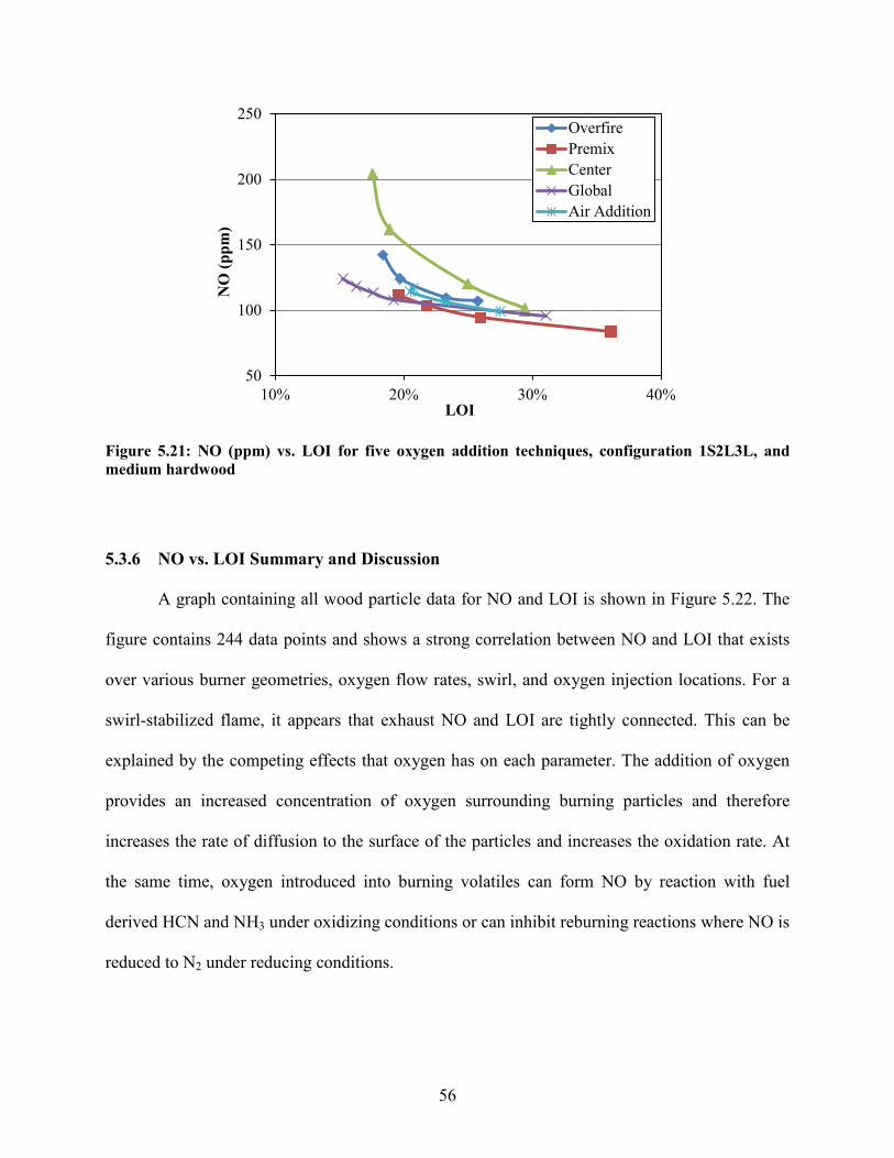
56

5.3.6 NO vs. LOI Summary and Discussion

A graph containing all wood particle data for NO and LOI is shown in Figure 5.22. The

figure contains 244 data points and shows a strong correlation between NO and LOI that exists

over various burner geometries, oxygen flow rates, swirl, and oxygen injection locations. For a

swirl-stabilized flame, it appears that exhaust NO and LOI are tightly connected. This can be

explained by the competing effects that oxygen has on each parameter. The addition of oxygen

provides an increased concentration of oxygen surrounding burning particles and therefore

increases the rate of diffusion to the surface of the particles and increases the oxidation rate. At

the same time, oxygen introduced into burning volatiles can form NO by reaction with fuel

derived HCN and NH3 under oxidizing conditions or can inhibit reburning reactions where NO is

reduced to N2 under reducing conditions.

50

100

150

200

250

10% 20% 30% 40%

NO

(ppm

)

LOI

OverfirePremixCenterGlobalAir Addition

Figure 5.21: NO (ppm) vs. LOI for five oxygen addition techniques, configuration 1S2L3L, and medium hardwood

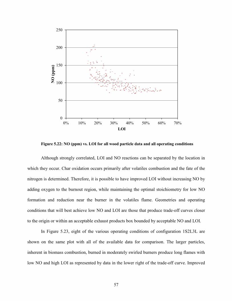
57

Although strongly correlated, LOI and NO reactions can be separated by the location in

which they occur. Char oxidation occurs primarily after volatiles combustion and the fate of the

nitrogen is determined. Therefore, it is possible to have improved LOI without increasing NO by

adding oxygen to the burnout region, while maintaining the optimal stoichiometry for low NO

formation and reduction near the burner in the volatiles flame. Geometries and operating

conditions that will best achieve low NO and LOI are those that produce trade-off curves closer

to the origin or within an acceptable exhaust products box bounded by acceptable NO and LOI.

In Figure 5.23, eight of the various operating conditions of configuration 1S2L3L are

shown on the same plot with all of the available data for comparison. The larger particles,

inherent in biomass combustion, burned in moderately swirled burners produce long flames with

low NO and high LOI as represented by data in the lower right of the trade-off curve. Improved

0

50

100

150

200

250

0% 10% 20% 30% 40% 50% 60% 70%

NO

(ppm

)

LOI

Figure 5.22: NO (ppm) vs. LOI for all wood particle data and all operating conditions

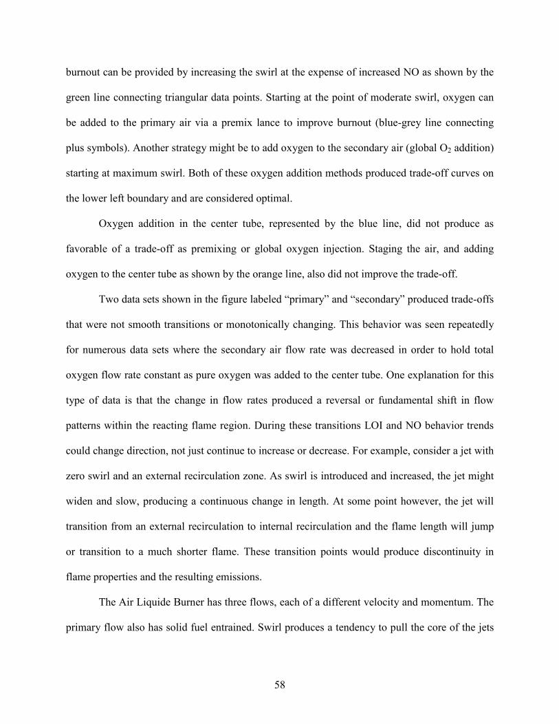
58

burnout can be provided by increasing the swirl at the expense of increased NO as shown by the

green line connecting triangular data points. Starting at the point of moderate swirl, oxygen can

be added to the primary air via a premix lance to improve burnout (blue-grey line connecting

plus symbols). Another strategy might be to add oxygen to the secondary air (global O2 addition)

starting at maximum swirl. Both of these oxygen addition methods produced trade-off curves on

the lower left boundary and are considered optimal.

Oxygen addition in the center tube, represented by the blue line, did not produce as

favorable of a trade-off as premixing or global oxygen injection. Staging the air, and adding

oxygen to the center tube as shown by the orange line, also did not improve the trade-off.

Two data sets shown in the figure labeled “primary” and “secondary” produced trade-offs

that were not smooth transitions or monotonically changing. This behavior was seen repeatedly

for numerous data sets where the secondary air flow rate was decreased in order to hold total

oxygen flow rate constant as pure oxygen was added to the center tube. One explanation for this

type of data is that the change in flow rates produced a reversal or fundamental shift in flow

patterns within the reacting flame region. During these transitions LOI and NO behavior trends

could change direction, not just continue to increase or decrease. For example, consider a jet with

zero swirl and an external recirculation zone. As swirl is introduced and increased, the jet might

widen and slow, producing a continuous change in length. At some point however, the jet will

transition from an external recirculation to internal recirculation and the flame length will jump

or transition to a much shorter flame. These transition points would produce discontinuity in

flame properties and the resulting emissions.

The Air Liquide Burner has three flows, each of a different velocity and momentum. The

primary flow also has solid fuel entrained. Swirl produces a tendency to pull the core of the jets

59

radially outward and produce an internal recirculation zone. At some axial location the

recirculation zone produces a stagnation point with incoming primary fuel and air running into

recirculated products. Each of the jets also has a velocity. When the velocity of one jet that is

initially higher than another jet is slowed, the shear layer between the two jets reverses. These

complex flow phenomena are difficult to predict based on basic flow rates and geometries.

Computational fluid dynamics (CFD) might be useful in identifying these transitions, but doing

so was beyond the scope of this work.

0

50

100

150

200

250

0% 10% 20% 30% 40% 50% 60%

NO

(ppm

)

LOI

Center GlobalSwirl PrimarySecondary PremixStaging All M. WoodAir Addition

Figure 5.23: NO (ppm) vs. LOI at eight different type of operating conditions for the medium hardwood and configuration 1S2L3L

60

5.4 NO-LOI Data for Straw and Fine Biomass

This section presents data for several operating conditions with wheat straw and fine

hardwood as the fuel. The results from these fuels are then compared to the medium hardwood

data.

5.4.1 Straw NO-LOI for Variable Swirl

Results for burner configuration 1S2L3S with center oxygen injection through a 25 mm

recessed tube are shown in Figure 5.24 for three swirl settings. Overall the data show a trade-off

between LOI and NO but the results are not as closely correlated as most of the medium

hardwood data. The maximum swirl case of 0.99 had a poor tradeoff curve and decreasing the

swirl to 0.77 decreased both NO and LOI. Visual observation of the flame suggested the lower

swirl setting maintained an active attached flame. At the lowest swirl, very low LOI rates were

achieved with 6-8 kg/hr of oxygen but the rest of the trade-off curve at low swirl was not as

favorable as medium swirl.

This trend where both NO and LOI improve as swirl was decreased was not observed in

the 1S2L3S configuration with medium particles as seen in Figure 5.12 and Figure 5.18. When

the medium hardwood was used in this same configuration, the flame was not as active and

attached as was the wheat straw. It is not clear why the wood flame appeared to be less active but

this suggests that combustion and the location of heat release which may have been significantly

different because of the difference in particle size between the two fuels may have an influence

on the fluid flow.

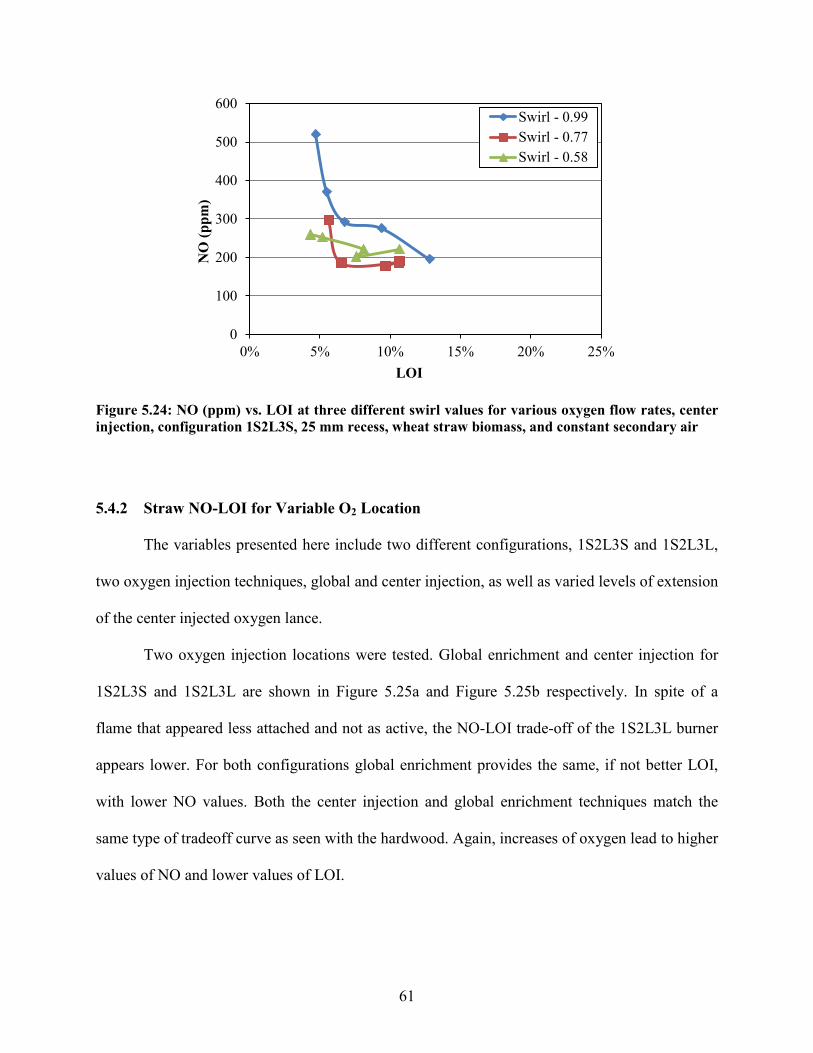
61

5.4.2 Straw NO-LOI for Variable O2 Location

The variables presented here include two different configurations, 1S2L3S and 1S2L3L,

two oxygen injection techniques, global and center injection, as well as varied levels of extension

of the center injected oxygen lance.

Two oxygen injection locations were tested. Global enrichment and center injection for

1S2L3S and 1S2L3L are shown in Figure 5.25a and Figure 5.25b respectively. In spite of a

flame that appeared less attached and not as active, the NO-LOI trade-off of the 1S2L3L burner

appears lower. For both configurations global enrichment provides the same, if not better LOI,

with lower NO values. Both the center injection and global enrichment techniques match the

same type of tradeoff curve as seen with the hardwood. Again, increases of oxygen lead to higher

values of NO and lower values of LOI.

0

100

200

300

400

500

600

0% 5% 10% 15% 20% 25%

NO

(ppm

)

LOI


Figure 5.24: NO (ppm) vs. LOI at three different swirl values for various oxygen flow rates, center injection, configuration 1S2L3S, 25 mm recess, wheat straw biomass, and constant secondary air

62

(a) 1S2L3S

(b) 1S2L3L

Two configurations are shown in Figure 5.26 where the height of the center tube was

varied between a recessed, flush, and extended position. These data were collected for the wheat

straw at maximum swirl for three O2 flow rates (0, 4, and 8 kg/hr) for configurations 1S2L3S,

Figure 5.26a, and 1S2L3L, Figure 5.26b. The influence of the center tube position in Figure

5.26a is not clear as most of the data are within the uncertainty of each other. For the

configuration 1S2L3L, the extended position has the largest range of data and the recessed

position has the tightest grouping. This trend is not repeated, however, for the 1S2L3S

configuration in Figure 5.26a. In this configuration, all three center tube positions yield very

similar results. From this figure one could possible argue that the center tube position does not

greatly affect the NO emissions or the LOI, but the 1S2L3L configuration results shown in

Figure 5.26b demonstrate that for no oxygen addition, the recessed tube produced lower LOI.

This is consistent with the possibility that the recessed tube provides a larger exit area and

therefore a lower velocity and momentum for the primary stream. This would allow the fuel

0

100

200

300

400

500

600

0% 5% 10% 15% 20% 25%

NO

(ppm

)

LOI

GlobalCenter

0

100

200

300

400

500

600

0% 5% 10% 15% 20% 25%

NO

(ppm

)

LOI

GlobalCenter

Figure 5.25: NO (ppm) vs. LOI at two oxygen injection locations (Global and Center), varying amounts of O2 flow rate, wheat straw biomass, maximum swirl, for burner configurations (a) 1S2L3S and (b) 1S2L3L

63

stream to have a lower momentum and higher potential for recirculation, thus lower fuel

penetration through the recirculation zone.

(a) 1S2L3S

(b) 1S2L3L

5.4.3 Straw Burned in Various Burner Configurations

Results for two configurations are shown in Figure 5.27 at their respective maximum

swirl value for varying levels of oxygen. Configuration 1S2L3L has lower NO values, but higher

LOI. Configuration 1S2L3S, was more attached and steadier than 1S2L3L and therefore

appeared to be the better flame based on visual observation.

0

100

200

300

400

500

600

0% 5% 10% 15% 20% 25%

NO

(ppm

)

LOI

25mm Rec.Flush25mm Ext.

0

100

200

300

400

500

600

0% 5% 10% 15% 20% 25%N

O (p

pm)

LOI

25mm Rec.Flush25mm Ext.

Figure 5.26: NO (ppm) vs. LOI at three different center tube extension heights, three O2 flow rates (0, 4, and 8 kg/hr) in tube 1, wheat straw biomass, maximum swirl, for burner configurations (a) 1S2L3S and (b) 1S2L3L

64

5.4.4 Fine Hardwood Results

Fine hardwood was used with configuration 1S2L3L under three swirl values and an

oxygen sweep in the center tube with a flush six-hole lance. This produced premixing of the fuel

and oxygen just before exiting the burner. NO versus LOI data are shown in Figure 5.28. At the

highest swirl value, the flame was very short and presumably appeared to be a type 2 flame

where the fuel did not penetrate through the recirculation zone but was attached to the burner and

was directed along the secondary air inlet flow. At maximum swirl, LOI decreased slightly with

the introduction of oxygen, but was accompanied by large increases in NO. Initially, at moderate

swirl, 1.11, the LOI improved greatly with small increases in NO at a low flow rate of oxygen.

As additional oxygen was added, the moderate swirl followed the highest swirl case. The lowest

swirl value, 0.84, resulted in higher amounts of LOI and lower values of NO. This figure shows

0

100

200

300

400

500

600

0% 5% 10% 15% 20% 25%

NO

(ppm

)

LOI

1S2L3L - 1.391S2L3S - 0.99

Figure 5.27: NO (ppm) vs. LOI at their respective maximum swirl value for various oxygen flow rates, center injection, wheat straw biomass, and constant secondary air

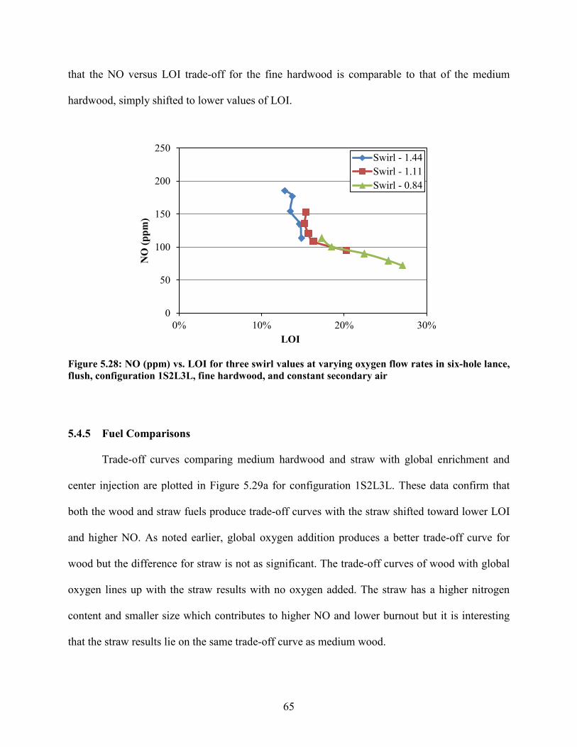
65

that the NO versus LOI trade-off for the fine hardwood is comparable to that of the medium

hardwood, simply shifted to lower values of LOI.

5.4.5 Fuel Comparisons

Trade-off curves comparing medium hardwood and straw with global enrichment and

center injection are plotted in Figure 5.29a for configuration 1S2L3L. These data confirm that

both the wood and straw fuels produce trade-off curves with the straw shifted toward lower LOI

and higher NO. As noted earlier, global oxygen addition produces a better trade-off curve for

wood but the difference for straw is not as significant. The trade-off curves of wood with global

oxygen lines up with the straw results with no oxygen added. The straw has a higher nitrogen

content and smaller size which contributes to higher NO and lower burnout but it is interesting

that the straw results lie on the same trade-off curve as medium wood.

0

50

100

150

200

250

0% 10% 20% 30%

NO

(ppm

)

LOI


Figure 5.28: NO (ppm) vs. LOI for three swirl values at varying oxygen flow rates in six-hole lance, flush, configuration 1S2L3L, fine hardwood, and constant secondary air

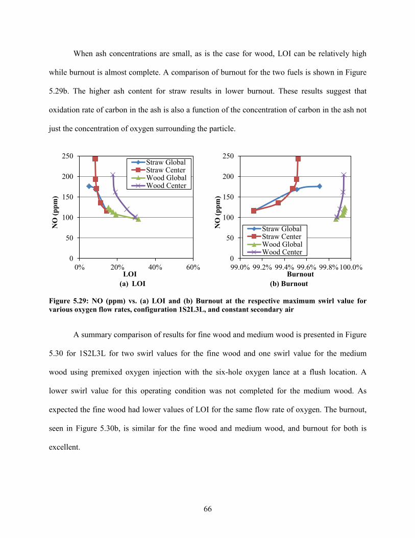
66

When ash concentrations are small, as is the case for wood, LOI can be relatively high

while burnout is almost complete. A comparison of burnout for the two fuels is shown in Figure

5.29b. The higher ash content for straw results in lower burnout. These results suggest that

oxidation rate of carbon in the ash is also a function of the concentration of carbon in the ash not

just the concentration of oxygen surrounding the particle.

(a) LOI

(b) Burnout

A summary comparison of results for fine wood and medium wood is presented in Figure

5.30 for 1S2L3L for two swirl values for the fine wood and one swirl value for the medium

wood using premixed oxygen injection with the six-hole oxygen lance at a flush location. A

lower swirl value for this operating condition was not completed for the medium wood. As

expected the fine wood had lower values of LOI for the same flow rate of oxygen. The burnout,

seen in Figure 5.30b, is similar for the fine wood and medium wood, and burnout for both is

excellent.

0

50

100

150

200

250

0% 20% 40% 60%

NO

(ppm

)

LOI

Straw GlobalStraw CenterWood GlobalWood Center

0

50

100

150

200

250

99.0% 99.2% 99.4% 99.6% 99.8% 100.0%

NO

(ppm

)

Burnout

Straw GlobalStraw CenterWood GlobalWood Center

Figure 5.29: NO (ppm) vs. (a) LOI and (b) Burnout at the respective maximum swirl value for various oxygen flow rates, configuration 1S2L3L, and constant secondary air

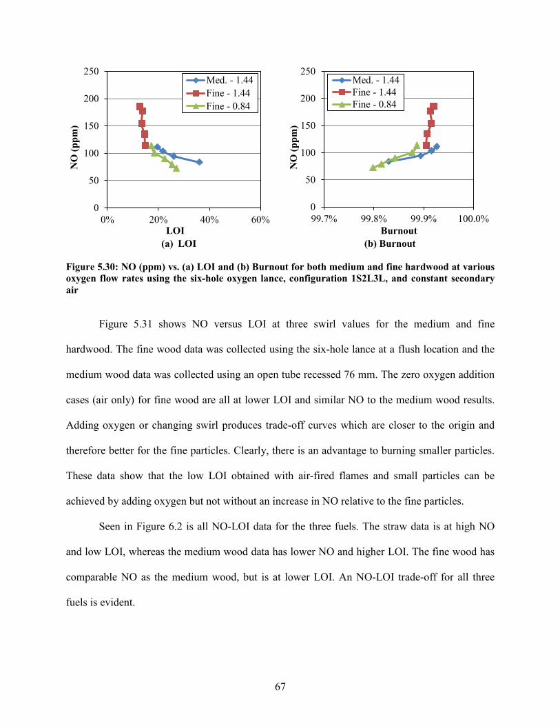
67

(a) LOI

(b) Burnout

Figure 5.31 shows NO versus LOI at three swirl values for the medium and fine

hardwood. The fine wood data was collected using the six-hole lance at a flush location and the

medium wood data was collected using an open tube recessed 76 mm. The zero oxygen addition

cases (air only) for fine wood are all at lower LOI and similar NO to the medium wood results.

Adding oxygen or changing swirl produces trade-off curves which are closer to the origin and

therefore better for the fine particles. Clearly, there is an advantage to burning smaller particles.

These data show that the low LOI obtained with air-fired flames and small particles can be

achieved by adding oxygen but not without an increase in NO relative to the fine particles.

Seen in Figure 6.2 is all NO-LOI data for the three fuels. The straw data is at high NO

and low LOI, whereas the medium wood data has lower NO and higher LOI. The fine wood has

comparable NO as the medium wood, but is at lower LOI. An NO-LOI trade-off for all three

fuels is evident.

0

50

100

150

200

250

0% 20% 40% 60%

NO

(ppm

)

LOI

Med. - 1.44Fine - 1.44Fine - 0.84

0

50

100

150

200

250

99.7% 99.8% 99.9% 100.0%

NO

(ppm

)

Burnout

Med. - 1.44Fine - 1.44Fine - 0.84

Figure 5.30: NO (ppm) vs. (a) LOI and (b) Burnout for both medium and fine hardwood at various oxygen flow rates using the six-hole oxygen lance, configuration 1S2L3L, and constant secondary air

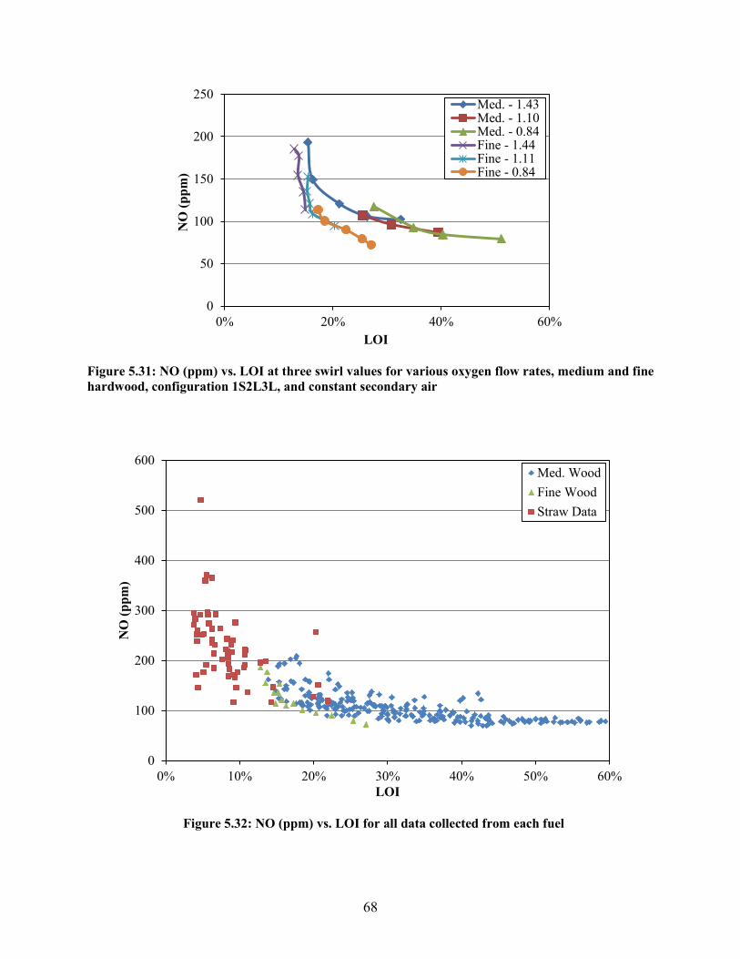
68

0

50

100

150

200

250

0% 20% 40% 60%

NO

(ppm

)

LOI

Med. - 1.43Med. - 1.10Med. - 0.84Fine - 1.44Fine - 1.11Fine - 0.84

0

100

200

300

400

500

600

0% 10% 20% 30% 40% 50% 60%

NO

(ppm

)

LOI

Med. WoodFine WoodStraw Data

Figure 5.31: NO (ppm) vs. LOI at three swirl values for various oxygen flow rates, medium and fine hardwood, configuration 1S2L3L, and constant secondary air

Figure 5.32: NO (ppm) vs. LOI for all data collected from each fuel

69

6 SCALING LAWS AND CORRELATION FOR NO AND LOI

The consistent albeit somewhat scattered correlation between LOI and NO over a broad

range of operating conditions, burner configurations, oxygen addition, and fuels suggests that

NO and LOI results might scale and be predicted by characteristics of the flow that are also

competing. For example, the residence time of fuel particles on the fuel rich side of the flame

zone and the residence time of particles in the post flame oxidation zone are two competing time

scales. As the flame lengthens and residence time in the flame zone increases, the time in the

particle oxidation zone decreases. While it is clear that the stoichiometry (oxidizer to fuel ratio)

is important, turbulent mixing and perhaps temperature of these zones are also significant. The

general trade-off of LOI and NO appears to be the first order effect with these other

considerations being secondary.

This chapter explores the ability to characterize the observed flames with scaling laws

and investigates the correlation of flame length obtained with these scaling laws to NO and LOI.

6.1 A Phenomenological Flame Model

A schematic diagram of a Type 1, swirl-stabilized, particle flame is shown in Figure 6.1.

While the aspect ratio of the flame may change based on swirl and flow rates, some essential

features of the flame are presented upon which scaling laws and correlations will be investigated.

The flame consists of a jet of solid fuel particles moving down the center of the flame which

enter with an initial primary fuel/air velocity, Vprim. This jet is surrounded by the secondary air

70

flow at axial velocity, Vsec. When center oxygen is present, a third jet exits the burner and flows

down the center of the fuel jet. These three jets can mix due to shearing at their interfaces and

therefore the relative velocities of these jets are important to mixing. Another mixing

characteristic of the jets is created by the swirl. The swirl creates a tangential velocity (not

shown) and a recirculation zone axial velocity which is shown by the vertical arrows pointing up

toward the burner on the inner edge of the flame. If the fuel jet has more momentum than the

recirculating flow, it will penetrate through the recirculating flow as shown and there will be no

stagnation point, making this a type 1 flame. Flames with a strong recirculation zone and

stagnation point are Type 2. The medium wood flames were visually observed to be Type 1.

To the left of the flame, three length and time scales are identified for the lift-off zone,

the volatiles flame zone, and the particle burnout zone. The lift-off length is the distance from

the burner exit to the ignition point of the flame. For this experiment, the ignition point was

taken to be the location where the flame luminosity was visually observed. The further the flame

is lifted from the burner, the more this point tends to move back and forth from the burner exit

and can therefore be difficult to define. The volatile flame length is the point at which volatile

combustion ends. In these experiments it was taken as the point at which luminous soot was no

longer observed. A more rigorous definition and measurement would be beneficial as this

position was also fluctuating and difficult to define. Near the end of the flame, the soot emission

decreases and it is difficult to determine what emission comes from soot and what comes from

solid particles. The final burnout length was not measured but was assumed to be the total

reactor length minus the flame length. At the reactor exit, the cold walls were expected to end

reactions relatively quickly, thus limiting the flame to the length of the reactor, 2.4 m.

71

Figure 6.1: Schematic diagram of a type 1, swirl stabilized, particle flame

72

6.1.1 Lift-Off and Flame Length Measurements

In this section, data is shown that compares lift-off length and flame length for three

burner configurations with medium wood particles. It should be noted that the data in this section

are only semi-quantitative because they were gathered from visual observation of the flame from

four port windows in the reactor. The data were collected visually as a first step at investigating

the value of more precise measurements which would require significantly greater effort.

In Figure 6.2, lengths for three separate configurations are shown at three swirl values

and varying amounts of oxygen injected in the center for the medium hardwood. These data

provide some indication of flame lengths for these conditions. In Figure 6.2a, configuration

1S2L3S is shown. In this figure the lowest lift corresponds with the highest amount of oxygen.

Thus with increased oxygen lift-off and volatile flame length decreases. The flame became

shorter with the addition of swirl and became more attached with the addition of oxygen. In

Figure 6.2b, configuration 1S2L3L, similar effects can be noted. The difference in this

configuration is the amount of lift when compared to 1S2L3S. Less lift can lead to less air

entrainment in the center and will decrease NO formation. When compared with 1S2L3L,

1S2L3S had similar LOI, but did have increased NO values as was seen in Figure 5.18. Lastly,

Figure 6.2c shows the lift versus length data for the configuration 1L2L3L. The attachment was

excellent, but the length was much longer than the other two configurations. This length of flame

made decreasing the LOI very difficult as the particles had very little time to oxidize. NO values

for the configuration 1L2L3L were very low due to the length of the fuel rich reducing zone.

Overall, both length and lift tend to decrease with increased swirl or oxygen.

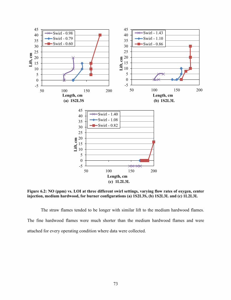
73

(a) 1S2L3S

(b) 1S2L3L

(c) 1L2L3L

The straw flames tended to be longer with similar lift to the medium hardwood flames.

The fine hardwood flames were much shorter than the medium hardwood flames and were

attached for every operating condition where data were collected.

-505

1015202530354045

50 100 150 200

Lift

, cm

Length, cm


-505

1015202530354045

50 100 150 200

Lift

, cm

Length, cm


-505

1015202530354045

50 100 150 200

Lift

, cm

Length, cm


Figure 6.2: NO (ppm) vs. LOI at three different swirl settings, varying flow rates of oxygen, center injection, medium hardwood, for burner configurations (a) 1S2L3S, (b) 1S2L3L and (c) 1L2L3L

74

6.1.2 Flame Length Model

A flame length model was created in attempt to determine parameters that might be used

to predict flame length and scaling parameters. The model will also be used to determine the

correlation between predicted flame length and NO and LOI.

A common method for predicting flame length is to determine the locations where fuel

and air mix to a stoichiometric composition. Using this approach, the flame length will occur at

axial position. Chen and Driscoll [24] used such an approach to predict the length of a swirling

gas flame. This approach was modified for a particle flame by first assuming that the volatile

mass and required air fuel ratio are that of the solid fuel. This could perhaps be improved by

using the volatile fraction from the proximate analysis but this was not done in this initial

attempt.

The constant 𝐶𝑎, as shown in Equation 6.1, is the stoichiometric air to fuel ratio where

�̇�𝑜𝑜 is the mass flow rate of oxidizer and �̇�𝑚𝑓𝑓𝑓 is the mass flow rate of fuel.

𝑐𝑎 = ��̇�𝑚𝑓𝑓𝑓

�̇�𝑜𝑜�

𝑎 (6.1)

These flow rates are related to geometric and flow parameters as shown in Equation 6.2.

The numerator represents the fuel flow entering through the primary annulus between the

primary tube diameter 𝑑𝑝 and the center tube diameter 𝑑𝑐, where 𝜌𝑚𝑚𝑜, is the primary fuel air

mixture density, 𝑉𝑃 is the primary mixture velocity, and 𝑌𝑚𝑓𝑓𝑓,𝑝 is the fuel mixture fraction of the

primary flow. The denominator consists of four terms each representing a flow of oxygen into

the flame. The first term, 𝑈𝑅𝑅, follows the nomenclature of Chen and Driscoll [24] and represents

the radial velocity along the axial circumference (𝜋𝐶𝐿𝑚) of the flame. 𝐿𝑚 is the flame length, 𝐶

the diameter of the recirculation zone core, 𝜌𝑎𝑓𝑐, is the density of the secondary air stream and

75

𝑌𝑂2,𝑎𝑓𝑐, is the mass fraction of O2 in the secondary stream. The magnitude of 𝑈𝑅𝑅 was determined

as a function of swirl, 𝑆, and secondary axial velocity, 𝑉𝑎𝑓𝑐, based on a correlation of the data

from Chen and Driscoll as shown in Equation 6.3. The second term in the denominator

represents oxygen mixing into the fuel jet due to the axial velocity difference between the fuel jet

and the secondary flow. The rate of mixing is assumed to be proportional to the absolute value of

the velocity difference of 𝑉𝑝 and 𝑉𝑎𝑓𝑐, which has been experimentally observed for turbulent

flames.

𝑐𝑎 =𝜌𝑚𝑚𝑜𝑉𝑝

𝜋4 �𝑑𝑝

2 − 𝑑𝑐2� ∗ 𝑌𝑚𝑓𝑓𝑓,𝑝

𝑌𝑂2,𝑎𝑓𝑐�𝜌𝑎𝑓𝑐𝜋𝐶𝐿𝑚𝑈𝑅𝑅𝑐2 + 𝜌𝑎𝑓𝑐�𝑉𝑝 − 𝑉𝑎𝑓𝑐�𝑑𝑝𝐿𝑚𝜋𝑐1� + �̇�𝑂2,𝑐 + �̇�𝑂2,𝑝 (6.2)

The third term in the denominator �̇�𝑂2,𝑐 is the flow rate of oxygen in the center tube. The

model assumes that all of the oxygen delivered from this tube is mixed into the fuel stream. This

may not be the case for higher flow rates of oxygen and will be checked by a calculation

discussed below. The final term in the denominator, �̇�𝑂2,𝑝, is the oxygen added to the primary

stream by premixing oxygen with the primary fuel and air.

𝑈𝑅𝑅 =0.2 ∗ 𝑆 ∗ 𝑉𝑎𝑓𝑐

0.2 + 𝑆 (6.3)

The flame length of a swirl-stabilized flame can be re-written as shown in Equation 6.4.

The constants 𝑐1 and 𝑐2 were found by minimizing a least squares difference between the

measured and predicted flame lengths for each fuel. With the constants calculated, the flame

length, 𝐿𝑚, for the turbulent, swirl-stabilized flame is found using Equation 6.4.

𝐿𝑚 =

�̇�𝑚𝑓𝑓𝑓𝑐𝑎

− �̇�𝑂2,𝑝 − �̇�𝑂2,𝑐

�𝜌𝑎𝑓𝑐𝜋𝐶𝑈𝑅𝑅𝑐2 + 𝜌�𝑉𝑝 − 𝑉𝑎𝑓𝑐�𝑑𝑝𝜋𝑐1�𝑌𝑂2,𝑎𝑓𝑐 (6.4)

76

Oxygen injected into the center tube can also form a separate flame at the stoichiometric

boundary between the fuel and oxygen. The flame length of the oxygen flame can be modeled in

the same way that the outer flame length is modeled as shown in Equation 6.5.

𝐿𝑂2 =𝑐𝑎 ∗ �̇�𝑂2

𝜌𝑚𝑚𝑜𝜋𝑑𝑐�𝑉𝑐 − 𝑉𝑝�𝑐1 ��̇�𝑚

�̇�𝑚𝑚𝑎�

(6.5)

This oxygen flame was calculated as a check. If this flame length is longer than the outer

flame length, the oxygen from the center flow will not be completely mixed into the fuel jet and

the model will under predict the flame length.

6.2 Flame Length Model – Measurement Comparison

The visual flame length measurements are compared to the calculated model flame length

in Figure 6.3. Given the relatively crude method of measurement and simple nature of the model,

the model appears to capture first order effects on the flame length.

0.0

0.5

1.0

1.5

2.0

2.5

0.0 0.5 1.0 1.5 2.0 2.5

Cal

cula

ted

Mod

el L

engt

h (m

)

Visually Estimated Length (m)

Med. WoodFine WoodStraw

Figure 6.3: Calculated Flame Length (m) vs. Visually Estimated Length (m) for all data collected separated by fuel

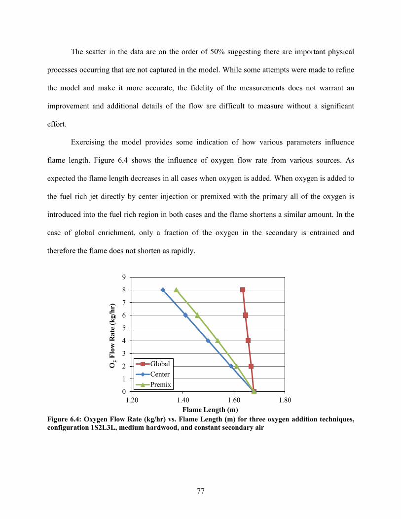
77

The scatter in the data are on the order of 50% suggesting there are important physical

processes occurring that are not captured in the model. While some attempts were made to refine

the model and make it more accurate, the fidelity of the measurements does not warrant an

improvement and additional details of the flow are difficult to measure without a significant

effort.

Exercising the model provides some indication of how various parameters influence

flame length. Figure 6.4 shows the influence of oxygen flow rate from various sources. As

expected the flame length decreases in all cases when oxygen is added. When oxygen is added to

the fuel rich jet directly by center injection or premixed with the primary all of the oxygen is

introduced into the fuel rich region in both cases and the flame shortens a similar amount. In the

case of global enrichment, only a fraction of the oxygen in the secondary is entrained and

therefore the flame does not shorten as rapidly.

0

1

2

3

4

5

6

7

8

9

1.20 1.40 1.60 1.80

O2 F

low

Rat

e (k

g/hr

)

Flame Length (m)

GlobalCenterPremix

Figure 6.4: Oxygen Flow Rate (kg/hr) vs. Flame Length (m) for three oxygen addition techniques, configuration 1S2L3L, medium hardwood, and constant secondary air

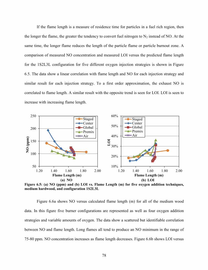
78

If the flame length is a measure of residence time for particles in a fuel rich region, then

the longer the flame, the greater the tendency to convert fuel nitrogen to N2 instead of NO. At the

same time, the longer flame reduces the length of the particle flame or particle burnout zone. A

comparison of measured NO concentration and measured LOI versus the predicted flame length

for the 1S2L3L configuration for five different oxygen injection strategies is shown in Figure

6.5. The data show a linear correlation with flame length and NO for each injection strategy and

similar result for each injection strategy. To a first order approximation, the exhaust NO is

correlated to flame length. A similar result with the opposite trend is seen for LOI. LOI is seen to

increase with increasing flame length.

(a) NO

(b) LOI

Figure 6.6a shows NO versus calculated flame length (m) for all of the medium wood

data. In this figure five burner configurations are represented as well as four oxygen addition

strategies and variable amounts of oxygen. The data show a scattered but identifiable correlation

between NO and flame length. Long flames all tend to produce an NO minimum in the range of

75-80 ppm. NO concentration increases as flame length decreases. Figure 6.6b shows LOI versus

50

100

150

200

250

1.20 1.40 1.60 1.80 2.00

NO

(ppm

)

Flame Length (m)

StagedCenterGlobalPremixAir

10%

20%

30%

40%

50%

60%

1.20 1.40 1.60 1.80 2.00

LO

I

Flame Length (m)

StagedCenterGlobalPremixAir

Figure 6.5: (a) NO (ppm) and (b) LOI vs. Flame Length (m) for five oxygen addition techniques, medium hardwood, and configuration 1S2L3L

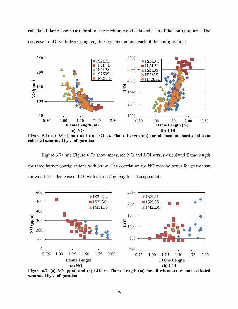
79

calculated flame length (m) for all of the medium wood data and each of the configurations. The

decrease in LOI with decreasing length is apparent among each of the configurations.

(a) NO

(b) LOI

Figure 6.7a and Figure 6.7b show measured NO and LOI versus calculated flame length

for three burner configurations with straw. The correlation for NO may be better for straw than

for wood. The decrease in LOI with decreasing length is also apparent.

(a) NO

(b) LOI

50

100

150

200

250

0.50 1.00 1.50 2.00 2.50

NO

(ppm

)

Flame Length (m)

1S2L3L1L2L3L1S2L3S1S2S3S1M2L3L

10%

20%

30%

40%

50%

60%

0.50 1.00 1.50 2.00 2.50L

OI

Flame Length (m)

1S2L3L1L2L3L1S2L3S1S2S3S1M2L3L

0

100

200

300

400

500

600

0.75 1.00 1.25 1.50 1.75 2.00

NO

(ppm

)

Flame Length

1S2L3L1S2L3S1M2L3S

0%

5%

10%

15%

20%

25%

0.75 1.00 1.25 1.50 1.75 2.00

LO

I

Flame Length

1S2L3L1S2L3S1M2L3S

Figure 6.6: (a) NO (ppm) and (b) LOI vs. Flame Length (m) for all medium hardwood data collected separated by configuration

Figure 6.7: (a) NO (ppm) and (b) LOI vs. Flame Length (m) for all wheat straw data collected separated by configuration

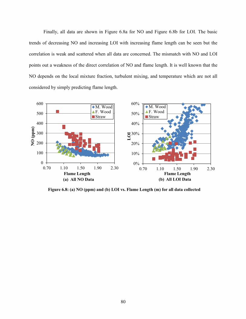
80

Finally, all data are shown in Figure 6.8a for NO and Figure 6.8b for LOI. The basic

trends of decreasing NO and increasing LOI with increasing flame length can be seen but the

correlation is weak and scattered when all data are concerned. The mismatch with NO and LOI

points out a weakness of the direct correlation of NO and flame length. It is well known that the

NO depends on the local mixture fraction, turbulent mixing, and temperature which are not all

considered by simply predicting flame length.

(a) All NO Data

(b) All LOI Data

0

100

200

300

400

500

600

0.70 1.10 1.50 1.90 2.30

NO

(ppm

)

Flame Length

M. WoodF. WoodStraw

0%

10%

20%

30%

40%

50%

60%

0.70 1.10 1.50 1.90 2.30

LO

I

Flame Length

M. WoodF. WoodStraw

Figure 6.8: (a) NO (ppm) and (b) LOI vs. Flame Length (m) for all data collected

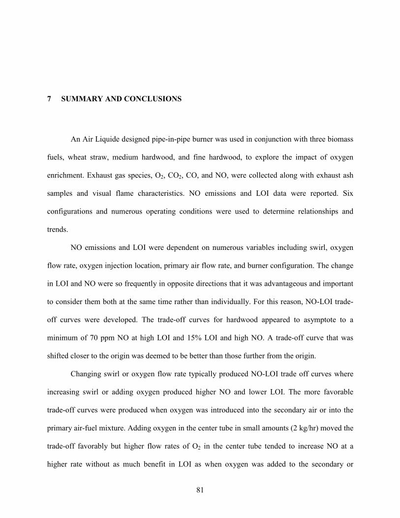
81

7 SUMMARY AND CONCLUSIONS

An Air Liquide designed pipe-in-pipe burner was used in conjunction with three biomass

fuels, wheat straw, medium hardwood, and fine hardwood, to explore the impact of oxygen

enrichment. Exhaust gas species, O2, CO2, CO, and NO, were collected along with exhaust ash

samples and visual flame characteristics. NO emissions and LOI data were reported. Six

configurations and numerous operating conditions were used to determine relationships and

trends.

NO emissions and LOI were dependent on numerous variables including swirl, oxygen

flow rate, oxygen injection location, primary air flow rate, and burner configuration. The change

in LOI and NO were so frequently in opposite directions that it was advantageous and important

to consider them both at the same time rather than individually. For this reason, NO-LOI trade-

off curves were developed. The trade-off curves for hardwood appeared to asymptote to a

minimum of 70 ppm NO at high LOI and 15% LOI and high NO. A trade-off curve that was

shifted closer to the origin was deemed to be better than those further from the origin.

Changing swirl or oxygen flow rate typically produced NO-LOI trade off curves where

increasing swirl or adding oxygen produced higher NO and lower LOI. The more favorable

trade-off curves were produced when oxygen was introduced into the secondary air or into the

primary air-fuel mixture. Adding oxygen in the center tube in small amounts (2 kg/hr) moved the

trade-off favorably but higher flow rates of O2 in the center tube tended to increase NO at a

higher rate without as much benefit in LOI as when oxygen was added to the secondary or

82

primary. Adding O2 radially or from a lance extended beyond the burner outlet also had a

tendency to produce a less favorable trade-off curve as oxygen was added. Decreasing the

amount of primary air or the primary air momentum produced a very favorable trade-off curve

where reductions in LOI were seen without a large increase in NO. The reduction of primary

flow was limited to the amount required to transport the fuel without plugging up the flow lines.

Oxygen injection was found to be an effective tool for LOI reduction, extending the

capacity of increased swirl. This was particularly true for larger fuel particles where LOI was

initially high and NO low when burned in air. The addition of oxygen was less useful for the fine

wood particles because LOI was already low and NO was high. Reducing swirl and adding

oxygen had a slightly better trade-off than swirl alone. Also, the addition of oxygen in the center

tube accompanied by reduced secondary flow designed to keep overall O2 concentration in the

exhaust constant had a negative effect on the trade-off curve where conditions existed in which

both NO and LOI increased.

It is believed the addition of oxygen generally had the effect of reducing the local

equivalence ratio, residence time, and size of fuel rich regions that reduce NO to N2 and inhibit

NO formation. Thus adding O2 was generally detrimental to NO. At the same time, it was

beneficial to LOI by providing a higher oxygen concentration in the burnout zone.

The actual volatile region equivalence ratio and change caused by O2 addition, swirl, or

burner configuration is difficult to predict as it is complicated by the existence of three jets

(center fuel, primary, and secondary) and swirl that interact and mix with each other. Swirl was

also assumed to cause increased O2 concentration or a leaner volatiles region. The reason that

center O2 injection produced an inferior trade-off curve to the other oxygen injection locations is

not clear. One potential explanation is that the center O2 jet was able in certain circumstances to

83

penetrate through the fuel rich recirculation zone. Because of the high temperature of pure O2

flames, thermal NO may become important. If not thermal NO, the NO formed between volatiles

and this O2 jet would have less opportunity for reburning if formed outside of the fuel rich jet

region.

The NO and LOI data appeared to correlate with observed flame lengths. As such a

relatively simple model was developed to predict flame length. The model requires two constants

to be selected based on a fit to at least two flame length data points. The model was moderately

successful in predicting the measured flame lengths and these flame lengths were found to

correlate the general trend of increasing NO with shorter flame length.

The burner configuration had a large impact on flame structure and characteristics.

Different configurations led to various primary and secondary velocities, which led to a wide

range of flame lengths and appearances. Configuration 1S2L3L was used primarily for hardwood

and produced a reasonably well attached Type 1 flame with the fuel jet penetrating through the

recirculation zone and producing a relatively high aspect ratio (long) flame. A change in variable

such as swirl or O2 flow rate that maintained the basic structure of this flame produced smoothly

changing, monotonic trade-off curves. Geometries that changed flow patterns caused NO-LOI

behavior that was erratic and less predictable. Configuration 1S2S3S along with 1L2L3L,

associated with high primary velocities, had long flames with LOI values that were difficult to

improve. Configuration 1S2S3S was skinny and elongated, whereas 1L2L3L was lazy, long, and

wide. It was found that configuration 1S2L3S led to better flame characteristics for the wheat

straw fuel. Recessing the center tube generally reduced flame length and acted as if the primary

momentum was slowed due to the wider pipe diameter opening to the primary flow just below

84

the center tube. Extending the center tube typically led to decreased mixing, lower NO and

higher LOI.

The straw fuel was compared to the medium hardwood with configurations 1S2L3L and

1S2L3S. Overall, the straw had a shifted NO versus LOI tradeoff curve toward higher values of

NO and lower values of LOI. This shifted curve is attributed to the ash and nitrogen content in

the fuel as well as the size distribution differences.

The fine hardwood fuel had comparable results to the medium hardwood, but with an NO

versus LOI tradeoff curve that had lower values of LOI. NO values were comparable to those

obtained with the medium wood. With the addition of oxygen or swirl LOI decreased at the cost

of increasing NO.

85

REFERENCES

[1] "Carbon Dioxide Emissions," 14 June 2012. [Online]. Available: http://www.epa.gov/climatechange/ghgemissions/gases/co2.html. [Accessed 5 April 2013].

[2] L. Baxter, "Biomass-Coal Co-Combustion: Opportunity for Affordable Renewable Energy," Fuel, vol. 84, pp. 1295-1302, 2005.

[3] R. Guerreo-Lemus and J. M. Martinez-Duart, Renewable Energies and CO2, London: Springer-Verlag, 2013.

[4] L. Baxter, "Solid Biofuels for Energy," in Solid Biofuels for Energy, Springer London, 2011, pp. 43-73.

[5] L. Baxter, "Co-Firing Overview," in Second World Conference and Exhibition on Biomass for Energy, Industry and Climate Protection, Rome, Italy, May 10-14, 2004.

[6] J. Koppejan, "Introduction and Overview of Technologies Applied Worldwide," in Second World Conference and Exhibition on Biomass for Energy, Industry and Climate Protection, Rome, Italy, May 10-14, 2004.

[7] "Nitrogen Dioxide," 15 August 2014. [Online]. Available: http://www.epa.gov/airquality/nitrogenoxides. [Accessed 24 February 2015].

[8] "Sulfer Dioxide," 15 August 2014. [Online]. Available: http://www.epa.gov/air/sulferdioxide. [Accessed 24 February 2015].

[9] S. Y. Luo, B. Xiao, Z. Q. Hu, S. M. Liu and Y. W. Guan, "Experimental Study on Oxygen-Enriched Combustion of Biomass Micro Fuel," Energy, vol. 34, pp. 1880-1884, 2009.

[10] M. Fang, D. Shen, Y. Li, C. Yu, Z. Yuo and K. Cen, "Kinetic Study on Pyrolysis and Combustion of Wood Under Different Oxygen Concentrations by Using TG-FTIR Analysis," Journal of Analytical and Applied Pyrolysis, vol. 77, no. 1, pp. 22-27, 2006.

[11] L. Bool, H. Kobayashi, K. Wu, D. Thompson, E. Eddings, O. Okerlund, J. Wendt, M. Cremer and D. Wang, "Oxygen for NOx Control - A Step Change Technology," in

86

Proceedings of the Nineteenth Annual International Pittsburg Coal Conference, Pittsburg, PA, 2002.

[12] L. E. Bool and S. Laux, "Oxygen Enhanced Combustion - A Demonstrated Option for NOx Control," in Proceedings of the 37th International Technical Conference on Clean Coal & Fuel Systems, Clearwater, FL, 2012.

[13] S. R. Turns, "Oxides of Nitrogen Formation," in An Introduction to Combustion Concepts and Applications, New York, The McGraw-Hill Companies, Inc., 2011, pp. 170-174.

[14] J. D. Thornock, "Burnout, NO, Flame Temperature, and Radiant Intensity from Oxygen-Enriched Combustion of a Hardwood Biomass," Brigham Young University, Provo, UT, 2013.

[15] P. Glarborg, A. D. Jensen and J. E. Johnsson, "Fuel Nitrogen Conversion in Solid Fuel Fired Systems," Progress in Energy and Combustion Science, vol. 29, no. 2, pp. 89-113, 2003.

[16] J. Wendt, "Mechanisms Governing the Formation and Destruction of NOx and Other Nitrogenous Species in Low NOx Coal Combustion Systems," Combustion Science and Technology, vol. 108, no. 4-6, pp. 323-344, 1995.

[17] W. P. Linak, J. A. McSorley, R. E. Hall, J. V. Ryan, R. K. Srivastava, J. Wendt and J. B. Mereb, "N2O Emissions From Fossil Fuel Combustion," in Proceedings of the 82nd Annual Meeting of the Air and Waste Management Association, Anaheim, CA, 1989.

[18] A. J. MacKrory and D. R. Tree, "Measurement of Nitrogen Evolution in a Staged Oxy-combustion Coal Flame," Fuel, no. 93, pp. 298-304, 2012.

[19] S. R. Turns, "Burning of Carbon," in An Introduction to Combustion Concepts and Applications, New York, The McGraw-Hill Companies, Inc., 2011, pp. 530-551.

[20] N. Dong, "Reducing Carbon-in-Ash," IEA Clean Coal Centre, London, 2010.

[21] J. Beer and N. Chigier, Combustion Aerodynamics, Essex: Applied Science Publishers LTD, 1972, pp. 109-114.

[22] M. Hupa, "International Flame Research Foundation," 24 January 2006. [Online]. Available: www.ffrc.fi/Liekkipaiva_2006/Liekkipaiva2006_IFRF_Today_HUPA.pdf. [Accessed 11 March 2015].

[23] A. Garg, "Trimming NOx from Furnaces," Chemical Engineering, vol. 99, no. 11, pp. 122-124, 1992.

87

[24] R.-H. Chen and J. F. Driscoll, "The Role of the Recirculation Vortex in Improving Fuel-Air Mixing within Swirling Flames," in The Combustion Institute, Pittsburgh, PA, 1988.

[25] T. Draper, D. Zeltner, D. R. Tree, Y. Xue, C. Periasamy, T. Kang and R. Tsiava, "Characterization of a Primary-Swirled, High Oxygen Participation Coal Flame: Flame Temperature, Emissivity, NO, and Burnout Measurements," Proceedings of the Combustion Institute, vol. 34, pp. 2779-2786, 2013.

[26] H. Kruczek, P. Raczka and A. Tatarek, "The Effect of Biomass on Pollutant Emission and Burnout in Co-Combustion," Combustion Science and Technology, vol. 178, no. 8, pp. 1511-1539, 2006.

[27] D. M. Boylan, "Southern Company Tests of Wood/Coal Cofiring in Pulverized Coal Units," Biomass and Bioenergy, vol. 10, no. 2-3, pp. 139-147, 1996.

[28] M. Pronobis, "Evaluation of the Influence of Biomass Co-Combustion on Boiler Furnace Slagging by Means of Fusibility Correlations," Biomass Bioenergy, vol. 28, pp. 375-283, 2005.

[29] S. Munir, W. Nimmo and B. M. Gibbs, "The Effect of Air Staged, Co-Combustion of Pulverised Coal and Biomass Blends on NOx Emissions and Combustion Efficiency," Fuel, vol. 90, pp. 126-135, 2011.

[30] H. Pawlak-Kruczek, M. Ostrycharczyk, M. Baranowski, M. Czerep and J. Zgora, "Co-Firing of Biomass with Pulverized Coal in Oxygen Enriched Atmosphere," Chemical and Process Engineering, vol. 34, no. 2, pp. 215-226, 2013.

[31] C. Yin, L. Rosendahl and S. K. Kaer, "Towards a Better Understanding of Biomass Suspension Co-Firing Impacts Via Investigating a Coal Flame and a Biomass Flame in a Swirl-Stabilized Burner Flow Reactor Under Same Conditions," Fuel Processing Technology, vol. 98, pp. 65-73, 2012.

[32] C. E. Baukal, Oxygen-Enhanced Combustion, Boca Raton, FL: CRC Press, 2013.

[33] M. B. Toftegaard, J. Brix, P. A. Jensen, P. Glarborg and A. D. Jensen, "Oxy-Fuel Combustion of Solid Fuels," Progress in Energy and Combustion Science, vol. 36, pp. 581-625, 2010.

[34] B. J. P. Buhre, L. K. Elliot, C. D. Sheng, R. P. Gupta and T. F. Wall, "Oxy-Fuel Combustion Technology for Coal Fired Power Generation," Progress in Energy and Combustion Science, vol. 31, pp. 283-307, 2005.

[35] T. Wall, Y. Liu, C. Spero, L. Elliott, S. Khare, R. Rathnam, F. Zeenathal, B. Moghtaderi, B. Buhre, C. Sheng, R. Gupta, T. Yamada, K. Makino and J. Yu, "An Overview of Oxy-Fuel Coal Combustion - State of the Art Research and Technology

88

Development," Chemical Engineering Research and Design, vol. 87, pp. 1003-1016, 2009.

[36] J. P. Smart and G. S. Riley, "Use of Oxygen Enriched Air Combustion to Enhance Combined Effectiveness of Oxyfuel Combustion and Post-Combustion Flue Gas Cleanup," Journal of the Energy Institute, vol. 85, no. 3, pp. 123-130, 2012.

[37] S. S. Daood, W. Nimmo, P. Edge and B. M. Gibbs, "Deep-Staged, Oxygen Enriched Combustion of Coal," Fuel, vol. 101, pp. 187-196, 2012.

[38] Y.-C. Chang, K.-K. Wu, C.-H. Chen and Y.-D. Chen, "Influences of Oxygen-Enriched Air on Combustion Characteristics of Industrial Furnaces," in 22nd International Symposium of Transport Phenomena, Delft, The Netherlands, 2011.

[39] W. Nimmo, S. S. Daood and B. M. Gibbs, "The Effect of O2 Enrichment on NOx Formation in Biomass Co-Fired Pulverised Coal Combustion," Fuel, vol. 89, pp. 2945-2952, 2010.

[40] J. Bai, C. Yu, L. Li, P. Wu, Z. Luo and M. Ni, "Experimental Study on the NO and N2O Formation Characteristics During Biomass Combustion," Energy and Fuels, no. 27, pp. 515-522, 2013.

[41] J. Riaza, M. V. Gil, L. Alvarez, C. Pevida, J. J. Pis and F. Rubiera, "Oxy-Fuel Combustion of Coal and Biomass Blends," Energy, vol. 41, no. 1, pp. 429-435, May 2012.

[42] O. Marin, F. Chatel-Pelage, M. U. Ghani, N. Perrin, R. Carty, G. R. Philo, H. Farzan and S. J. Vecci, "Low-Oxygen Enrichment in Coal-Fired Utility Boilers," in The 28th International Technical Conference on Coal Utilization & Fuel Systems, Clearwater, FL, 2003.

[43] D. Zeltner, "NO, Burnout, Flame Temperature, Emissivity, and Radiation Intensity from Oxycombustion Flames," Brigham Young University, Provo, UT, 2012.

[44] B. Damstedt, J. M. Pederson, D. Hansen, T. Knighton, J. Jones, C. Christensen, L. Baxter and D. Tree, "Biomass Cofiring Impacts on Flame Structure and Emissions," Proceedings of the Combustion Institute, vol. 31, pp. 2813-2820, 2007.

[45] T. A. Reeder, "Corrosion-related Gas Measurements and Analysis for a Suite of Coals in Staged Pulverized Coal Combustion," Brigham Young University, Provo, UT, 2010.

[46] S. C. Chamberlain, "Measurement and Analysis of Gas Composition in a Staged and Unstaged Oxy-Fired Pulverized Coal Reactor with Warm Flue Gas Recycle," Brigham Young University, Provo, UT, 2012.

89

APPENDIX A: AIR LIQUIDE BURNER SWIRL

A.1 Swirl Calculations

Swirl, 𝑆, has been studied by Beer and Chigier [21] and is defined in Equation A.1, where

𝐺𝜑, is axial flux of angular momentum in Equation A.2 (shown is for a three concentric pipe in

pipe burner), 𝐺𝑧 is the axial flux of axial momentum in Equation A.3, and 𝑅 is the burner radius,

for this case 𝑅5.

𝑆 = 𝐺𝜑

𝐺𝑧𝑅 (A.1)

𝐺𝜑 = � (𝐶𝜌𝐵𝑟)2𝜋𝐶𝑑𝐶𝑎1

0+ � (𝐶𝜌𝐵𝑟)2𝜋𝐶𝑑𝐶

𝑎3

𝑎2

+ � (𝐶𝜌𝐵𝑟)2𝜋𝐶𝑑𝐶𝑎5

𝑎4

(A.2)

𝐺𝑧 = � 𝜌𝐵22𝜋𝐶𝑑𝐶𝑎1

0+ � 𝜌𝐵22𝜋𝐶𝑑𝐶

𝑎3

𝑎2

+ � 𝜌𝐵22𝜋𝐶𝑑𝐶𝑎5

𝑎4

+ � 𝑝𝑑𝑝 (A.3)

In these equations, 𝐵 and 𝑟 are the axial and tangential velocities respectively, 𝑝 is the

flow area, 𝑝 is the static pressure, 𝐶 is the radius, and 𝜌 is the flow density. 𝐺𝜑 can be

approximated, Equation A.4, as can 𝐺𝑧, Equation A.5, assuming a uniform velocity profile and

constant static pressure across the flow area.

𝐺𝜑 = �23

𝜋𝜌𝐵𝑟(𝐶𝑚+13 − 𝐶𝑚

3)� (A.4)

𝐺𝑧 = [𝜌𝐵2𝜋(𝐶𝑚+12 − 𝐶𝑚

2)] (A.5)

Total swirl was calculated in a similar fashion where the sum of all tangential momentum

was divided by the product of the radius of the secondary flow and the sum of all axial

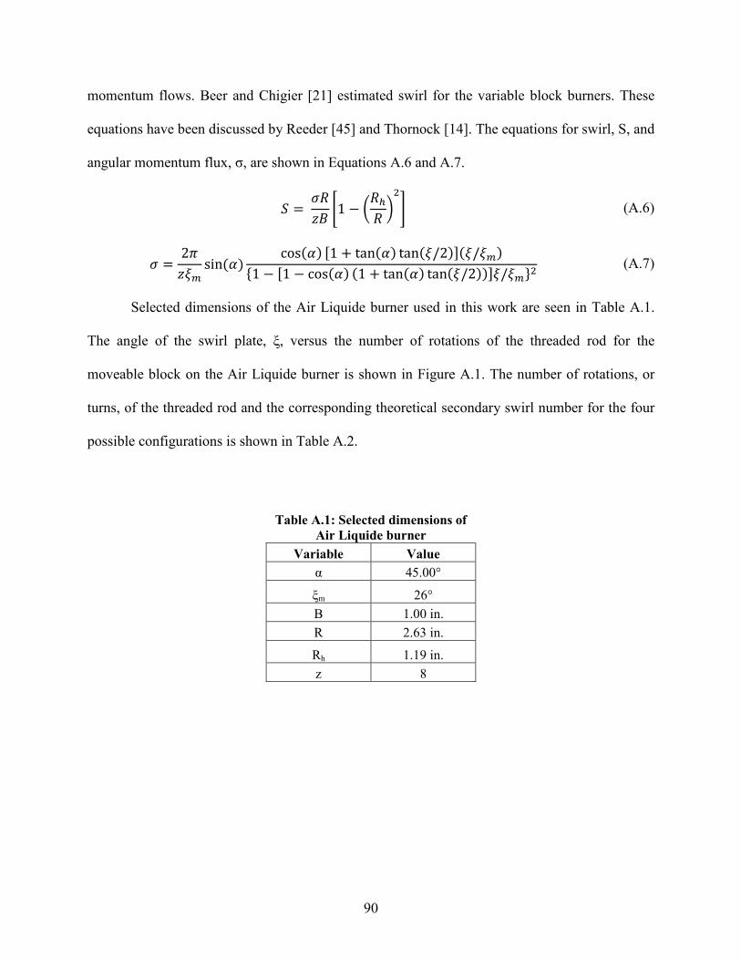
90

momentum flows. Beer and Chigier [21] estimated swirl for the variable block burners. These

equations have been discussed by Reeder [45] and Thornock [14]. The equations for swirl, S, and

angular momentum flux, σ, are shown in Equations A.6 and A.7.

𝑆 = 𝜎𝑅𝑧𝐵

�1 − �𝑅ℎ

𝑅�

2

� (A.6)

𝜎 =2𝜋

𝑧𝜉𝑚sin(𝛼)

cos(𝛼) [1 + tan(𝛼) tan(𝜉/2)](𝜉/𝜉𝑚){1 − [1 − cos(𝛼) (1 + tan(𝛼) tan(𝜉/2))]𝜉/𝜉𝑚}2 (A.7)

Selected dimensions of the Air Liquide burner used in this work are seen in Table A.1.

The angle of the swirl plate, ξ, versus the number of rotations of the threaded rod for the

moveable block on the Air Liquide burner is shown in Figure A.1. The number of rotations, or

turns, of the threaded rod and the corresponding theoretical secondary swirl number for the four

possible configurations is shown in Table A.2.

Table A.1: Selected dimensions of Air Liquide burner

Variable Value α 45.00°

ξm 26° B 1.00 in. R 2.63 in.

Rh 1.19 in. z 8

91

Table A.2: Multiple rod rotations matched with corresponding theoretical secondary

swirl numbers for the four possible configurations

Turns 2L3L 2S3L 2L3S 2S3S 0-1.5 1.473 1.610 1.031 1.200

2 1.441 1.574 1.008 1.173 3 1.372 1.499 0.960 1.117 4 1.298 1.418 0.909 1.057 5 1.219 1.332 0.853 0.993 6 1.135 1.240 0.795 0.925 7 1.047 1.144 0.733 0.853 8 0.955 1.044 0.669 0.778 9 0.861 0.940 0.602 0.701 10 0.763 0.834 0.534 0.622 11 0.664 0.726 0.465 0.541 12 0.565 0.617 0.396 0.460 13 0.466 0.509 0.326 0.380 14 0.369 0.403 0.258 0.301 15 0.275 0.300 0.192 0.224 16 0.184 0.201 0.129 0.150 17 0.099 0.108 0.069 0.080 18 0.019 0.021 0.013 0.015

y = -0.034x2 - 0.8737x + 27.272

0

5

10

15

20

25

30

0 5 10 15 20

ξ (d

egre

es)

Rotations of Threaded Rod

Figure A.1: Angle ξ (degrees) vs. Rotations of Threaded Rod for Air Liquide burner

92

A.2 Axial Profile Data

A hot wire anemometer was used to collect velocity data at the burner plane exit. This

was collected radially for 2 burner configurations, 2L3S and 2L3L, and for 2 flow rates, 158 and

170 kg/hr. Figure A.2 shows axial and tangential velocity measurements for secondary flow rates

of 158 and 170 kg/hr for configuration 2L3S. Axial velocity measurements were taken with the

wire in a horizontal position and tangential velocity measurements were taken with the wire in a

vertical position. Axial velocity measurements reveal a fairly uniform profile in the radial

direction. Maximum swirl had the highest axial velocity and decreasing the swirl also decreased

the axial velocity. For the tangential direction, maximum swirl saw higher velocities in the

center, whereas lower swirl values had more of a uniform velocity profile. These trends were

consistent for both flow rates.

Figure A.3 shows axial and tangential velocity measurements for secondary flow rates of

158 and 170 kg/hr for configuration 2L3L. This configuration is dramatically different from

2L3S. In this configuration at maximum swirl the axial velocity increased with an increase in

radial distance away from the center. The slope of this line decreased with a decrease in swirl

until it became level at no swirl. The tangential velocity for both flow rates showed identical

trends, with the higher swirl values achieving the highest velocity measurements in the center

and becoming slower at the tube walls.

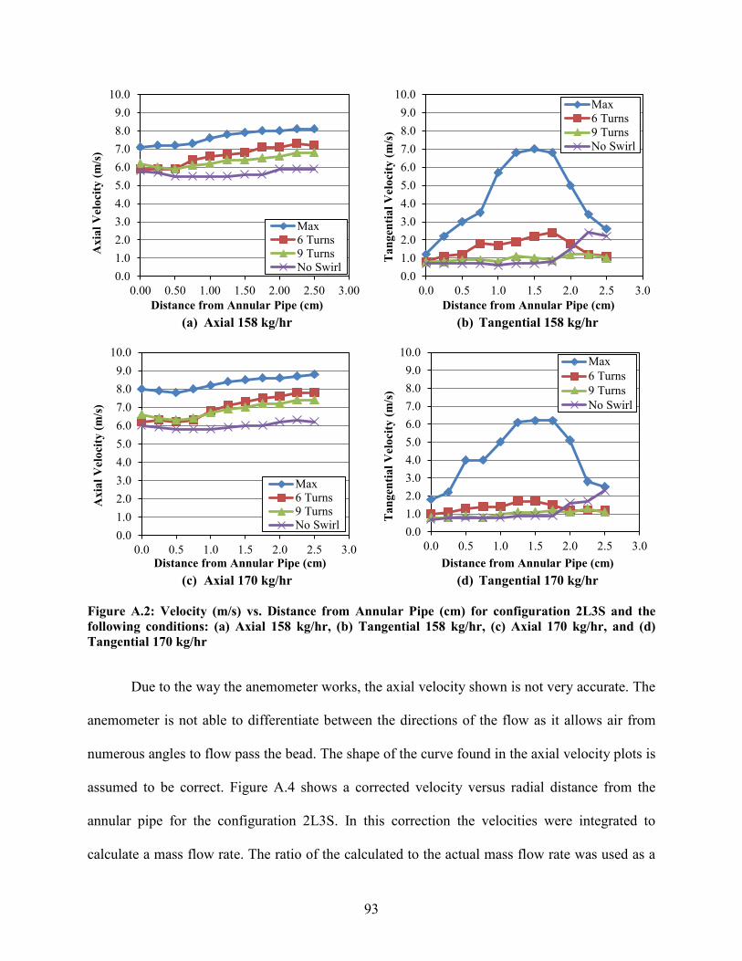
93

(a) Axial 158 kg/hr

(b) Tangential 158 kg/hr

(c) Axial 170 kg/hr

(d) Tangential 170 kg/hr

Due to the way the anemometer works, the axial velocity shown is not very accurate. The

anemometer is not able to differentiate between the directions of the flow as it allows air from

numerous angles to flow pass the bead. The shape of the curve found in the axial velocity plots is

assumed to be correct. Figure A.4 shows a corrected velocity versus radial distance from the

annular pipe for the configuration 2L3S. In this correction the velocities were integrated to

calculate a mass flow rate. The ratio of the calculated to the actual mass flow rate was used as a

0.01.02.03.04.05.06.07.08.09.0

10.0

0.00 0.50 1.00 1.50 2.00 2.50 3.00

Axi

al V

eloc

ity (m

/s)

Distance from Annular Pipe (cm)

Max6 Turns9 TurnsNo Swirl

0.01.02.03.04.05.06.07.08.09.0

10.0

0.0 0.5 1.0 1.5 2.0 2.5 3.0

Tan

gent

ial V

eloc

ity (m

/s)



0.01.02.03.04.05.06.07.08.09.0

10.0

0.0 0.5 1.0 1.5 2.0 2.5 3.0

Axi

al V

eloc

ity (m

/s)


Max6 Turns9 TurnsNo Swirl 0.0

1.02.03.04.05.06.07.08.09.0

10.0

0.0 0.5 1.0 1.5 2.0 2.5 3.0

Tan

gent

ial V

eloc

ity (m

/s)



Figure A.2: Velocity (m/s) vs. Distance from Annular Pipe (cm) for configuration 2L3S and the following conditions: (a) Axial 158 kg/hr, (b) Tangential 158 kg/hr, (c) Axial 170 kg/hr, and (d) Tangential 170 kg/hr

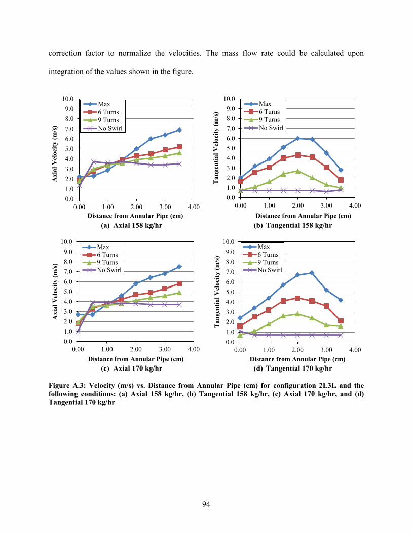
94

correction factor to normalize the velocities. The mass flow rate could be calculated upon

integration of the values shown in the figure.

(a) Axial 158 kg/hr


(c) Axial 170 kg/hr


0.01.02.03.04.05.06.07.08.09.0

10.0

0.00 1.00 2.00 3.00 4.00

Axi

al V

eloc

ity (m

/s)



0.01.02.03.04.05.06.07.08.09.0

10.0

0.00 1.00 2.00 3.00 4.00T

ange

ntia

l Vel

ocity

(m/s

) Distance from Annular Pipe (cm)


0.01.02.03.04.05.06.07.08.09.0

10.0

0.00 1.00 2.00 3.00 4.00

Axi

al V

eloc

ity (m

/s)



0.01.02.03.04.05.06.07.08.09.0

10.0

0.00 1.00 2.00 3.00 4.00

Tan

gent

ial V

eloc

ity (m

/s)



Figure A.3: Velocity (m/s) vs. Distance from Annular Pipe (cm) for configuration 2L3L and the following conditions: (a) Axial 158 kg/hr, (b) Tangential 158 kg/hr, (c) Axial 170 kg/hr, and (d) Tangential 170 kg/hr

95

(a) Axial 158 kg/hr


(c) Axial 170 kg/hr


This correction factor was calculated using only the axial velocity data, but was then

applied to both the axial and tangential velocity plots. Shown in Figure A.5 is the corrected

velocity versus radial distance from the annular pipe for the configuration 2L3L.

It should be noted however, that the collected values and the corrected values do not

account for the temperature. All radial velocity profile tests were completed at room temperature.

However, collection of combustion data took place with the secondary air temperature heated to

0123456789

10

0.00 0.50 1.00 1.50 2.00 2.50 3.00

Axi

al V

eloc

ity (m

/s)



0123456789

10

0.0 0.5 1.0 1.5 2.0 2.5 3.0

Tan

gent

ial V

eloc

ity (m

/s)



0123456789

10

0.0 0.5 1.0 1.5 2.0 2.5 3.0

Axi

al V

eloc

ity (m

/s)


Max6 Turns9 TurnsNo Swirl 0

123456789

10

0.0 0.5 1.0 1.5 2.0 2.5 3.0

Tan

gent

ial V

eloc

ity (m

/s)



Figure A.4: Corrected Velocity (m/s) vs. Distance from Annular Pipe (cm) for configuration 2L3S and the following conditions: (a) Axial 158 kg/hr, (b) Tangential 158 kg/hr, (c) Axial 170 kg/hr, and (d) Tangential 170 kg/hr

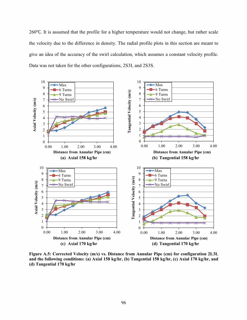
96

260℃. It is assumed that the profile for a higher temperature would not change, but rather scale

the velocity due to the difference in density. The radial profile plots in this section are meant to

give an idea of the accuracy of the swirl calculation, which assumes a constant velocity profile.

Data was not taken for the other configurations, 2S3L and 2S3S.

(a) Axial 158 kg/hr


(c) Axial 170 kg/hr


0123456789

10

0.00 1.00 2.00 3.00 4.00

Axi

al V

eloc

ity (m

/s)



0123456789

10

0.00 1.00 2.00 3.00 4.00

Tan

gent

ial V

eloc

ity (m

/s)



0123456789

10

0.00 1.00 2.00 3.00 4.00

Axi

al V

eloc

ity (m

/s)



0123456789

10

0.00 1.00 2.00 3.00 4.00

Tan

gent

ial V

eloc

ity (m

/s)



Figure A.5: Corrected Velocity (m/s) vs. Distance from Annular Pipe (cm) for configuration 2L3L and the following conditions: (a) Axial 158 kg/hr, (b) Tangential 158 kg/hr, (c) Axial 170 kg/hr, and (d) Tangential 170 kg/hr

97

APPENDIX B: DATA FROM REACTOR

NOx can be converted from ppm to lb/MMBtu. For the reader’s information, using the

reactor in this work with medium hardwood and accounting for an energy conversion efficiency

of 33%, 125 ppm is calculated to be roughly 0.385 lb NO/MMBtu. For the fine hardwood and

wheat straw, 125 ppm is calculated to be about 0.412 and 0.383 lb NO/MMBtu respectively.

B.1 Uncertainty Analysis

There are a variety of sources for error in data, including precision error, bias error, and

operating variability. Precision error refers to error associated with a range of values, or the

closeness of agreement, wherein the data lies. Bias error refers to error that is an offset from true

values or the trueness of data. Daily calibration of instruments was done to ensure that bias error

was kept as low as possible. Unquantified bias error includes changes in the flow rate and

pressure of the sample line and the unsteady flow of ash from the cyclone. Operating variability

refers to error in repeatability of data due to the method or procedure of experiments and

fluctuations due to the nature of the system setup.

In the operation of the BFR and in working with combustion, repeatability of the

experiments becomes a major factor in error. Much effort is done ensuring the method of

operation is consistent, instrumentation is properly calibrated, and that flow rates are constant.

Upon repeated conditions, questions are raised as to why or why not data is in agreement with

previous data. The temperature of the walls and pressure within the reactor, the consistency of

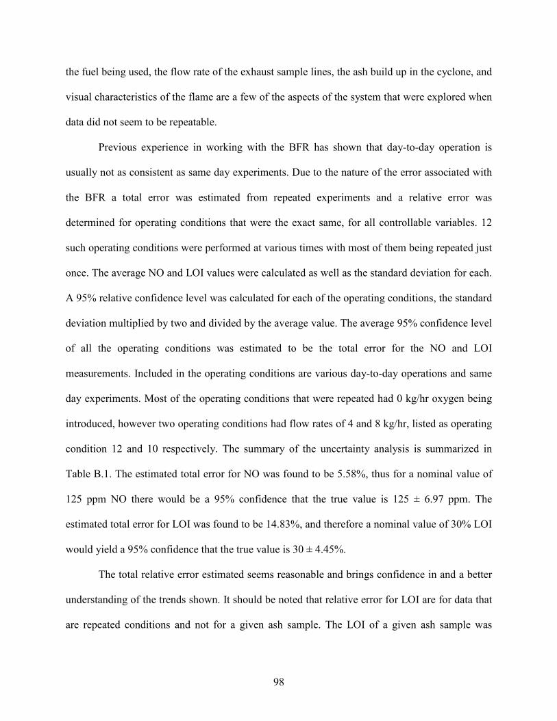
98

the fuel being used, the flow rate of the exhaust sample lines, the ash build up in the cyclone, and

visual characteristics of the flame are a few of the aspects of the system that were explored when

data did not seem to be repeatable.

Previous experience in working with the BFR has shown that day-to-day operation is

usually not as consistent as same day experiments. Due to the nature of the error associated with

the BFR a total error was estimated from repeated experiments and a relative error was

determined for operating conditions that were the exact same, for all controllable variables. 12

such operating conditions were performed at various times with most of them being repeated just

once. The average NO and LOI values were calculated as well as the standard deviation for each.

A 95% relative confidence level was calculated for each of the operating conditions, the standard

deviation multiplied by two and divided by the average value. The average 95% confidence level

of all the operating conditions was estimated to be the total error for the NO and LOI

measurements. Included in the operating conditions are various day-to-day operations and same

day experiments. Most of the operating conditions that were repeated had 0 kg/hr oxygen being

introduced, however two operating conditions had flow rates of 4 and 8 kg/hr, listed as operating

condition 12 and 10 respectively. The summary of the uncertainty analysis is summarized in

Table B.1. The estimated total error for NO was found to be 5.58%, thus for a nominal value of

125 ppm NO there would be a 95% confidence that the true value is 125 ± 6.97 ppm. The

estimated total error for LOI was found to be 14.83%, and therefore a nominal value of 30% LOI

would yield a 95% confidence that the true value is 30 ± 4.45%.

The total relative error estimated seems reasonable and brings confidence in and a better

understanding of the trends shown. It should be noted that relative error for LOI are for data that

are repeated conditions and not for a given ash sample. The LOI of a given ash sample was

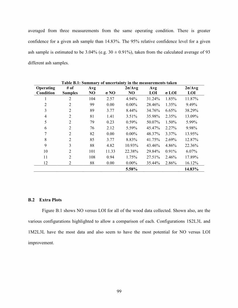
99

averaged from three measurements from the same operating condition. There is greater

confidence for a given ash sample than 14.83%. The 95% relative confidence level for a given

ash sample is estimated to be 3.04% (e.g. 30 ± 0.91%), taken from the calculated average of 93

different ash samples.

Table B.1: Summary of uncertainty in the measurements taken Operating Condition

# of Samples

Avg NO σ NO

2σ/Avg NO

Avg LOI σ LOI

2σ/Avg LOI

1 2 104 2.57 4.94% 31.24% 1.85% 11.87% 2 2 99 0.00 0.00% 28.46% 1.35% 9.49% 3 2 89 3.77 8.44% 34.76% 6.65% 38.29% 4 2 81 1.41 3.51% 35.98% 2.35% 13.09% 5 2 79 0.23 0.59% 50.07% 1.50% 5.99% 6 2 76 2.12 5.59% 45.47% 2.27% 9.98% 7 2 82 0.00 0.00% 48.37% 3.37% 13.95% 8 2 85 3.77 8.83% 41.75% 2.69% 12.87% 9 3 88 4.82 10.93% 43.46% 4.86% 22.36% 10 2 101 11.33 22.38% 29.84% 0.91% 6.07% 11 2 108 0.94 1.75% 27.51% 2.46% 17.89% 12 2 88 0.00 0.00% 35.44% 2.86% 16.12%

5.58%

14.83%

B.2 Extra Plots

Figure B.1 shows NO versus LOI for all of the wood data collected. Shown also, are the

various configurations highlighted to allow a comparison of each. Configurations 1S2L3L and

1M2L3L have the most data and also seem to have the most potential for NO versus LOI

improvement.

100

(a) All Hardwood Data

(b) 1S2L3L

(c) 1S2S3S

(d) 1S2L3S

(e) 1M2L3L

(f) 1L2L3L

0

50

100

150

200

250

0% 20% 40% 60%

NO

(ppm

)

LOI

Med. WoodFine Wood

0

50

100

150

200

250

0% 20% 40% 60%

NO

(ppm

)

LOI

Wood Data1S2L3L

0

50

100

150

200

250

0% 20% 40% 60%

NO

(ppm

)

LOI

Wood Data1S2S3S

0

50

100

150

200

250

0% 20% 40% 60%

NO

(ppm

)

LOI

Wood Data1S2L3S

0

50

100

150

200

250

0% 20% 40% 60%

NO

(ppm

)

LOI

Wood Data1M2L3L

0

50

100

150

200

250

0% 20% 40% 60%

NO

(ppm

)

LOI

Wood Data1L2L3L

Figure B.1: NO (ppm) vs. LOI showing (a) All Hardwood Data and configurations (b) 1S2L3L, (c) 1S2S3S, (d) 1S2L3S, (e) 1M2L3L, and (f) 1L2L3L

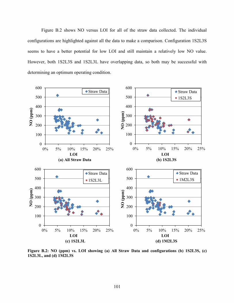
101

Figure B.2 shows NO versus LOI for all of the straw data collected. The individual

configurations are highlighted against all the data to make a comparison. Configuration 1S2L3S

seems to have a better potential for low LOI and still maintain a relatively low NO value.

However, both 1S2L3S and 1S2L3L have overlapping data, so both may be successful with

determining an optimum operating condition.

(a) All Straw Data

(b) 1S2L3S

(c) 1S2L3L

(d) 1M2L3S

0

100

200

300

400

500

600

0% 5% 10% 15% 20% 25%

NO

(ppm

)

LOI

Straw Data

0

100

200

300

400

500

600

0% 5% 10% 15% 20% 25%

NO

(ppm

)

LOI

Straw Data1S2L3S

0

100

200

300

400

500

600

0% 5% 10% 15% 20% 25%

NO

(ppm

)

LOI

Straw Data1S2L3L

0

100

200

300

400

500

600

0% 5% 10% 15% 20% 25%

NO

(ppm

)

LOI

Straw Data1M2L3S

Figure B.2: NO (ppm) vs. LOI showing (a) All Straw Data and configurations (b) 1S2L3S, (c) 1S2L3L, and (d) 1M2L3S

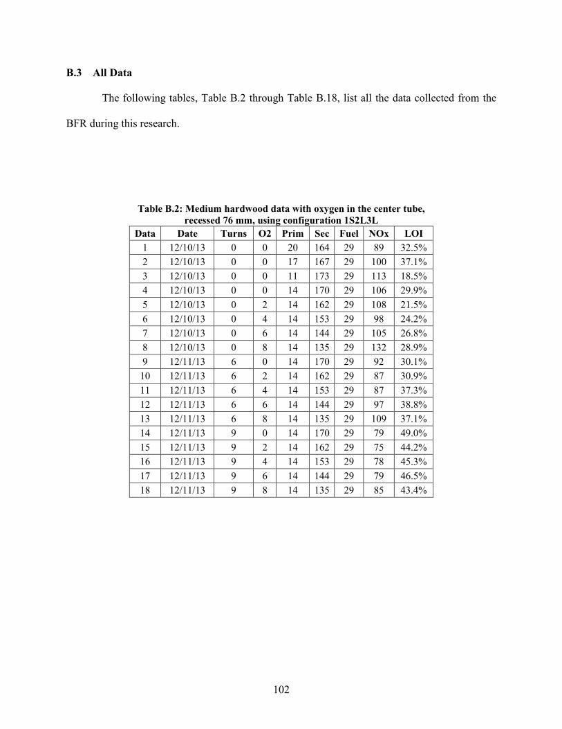
102

B.3 All Data

The following tables, Table B.2 through Table B.18, list all the data collected from the

BFR during this research.

Table B.2: Medium hardwood data with oxygen in the center tube, recessed 76 mm, using configuration 1S2L3L

Data Date Turns O2 Prim Sec Fuel NOx LOI 1 12/10/13 0 0 20 164 29 89 32.5% 2 12/10/13 0 0 17 167 29 100 37.1% 3 12/10/13 0 0 11 173 29 113 18.5% 4 12/10/13 0 0 14 170 29 106 29.9% 5 12/10/13 0 2 14 162 29 108 21.5% 6 12/10/13 0 4 14 153 29 98 24.2% 7 12/10/13 0 6 14 144 29 105 26.8% 8 12/10/13 0 8 14 135 29 132 28.9% 9 12/11/13 6 0 14 170 29 92 30.1% 10 12/11/13 6 2 14 162 29 87 30.9% 11 12/11/13 6 4 14 153 29 87 37.3% 12 12/11/13 6 6 14 144 29 97 38.8% 13 12/11/13 6 8 14 135 29 109 37.1% 14 12/11/13 9 0 14 170 29 79 49.0% 15 12/11/13 9 2 14 162 29 75 44.2% 16 12/11/13 9 4 14 153 29 78 45.3% 17 12/11/13 9 6 14 144 29 79 46.5% 18 12/11/13 9 8 14 135 29 85 43.4%

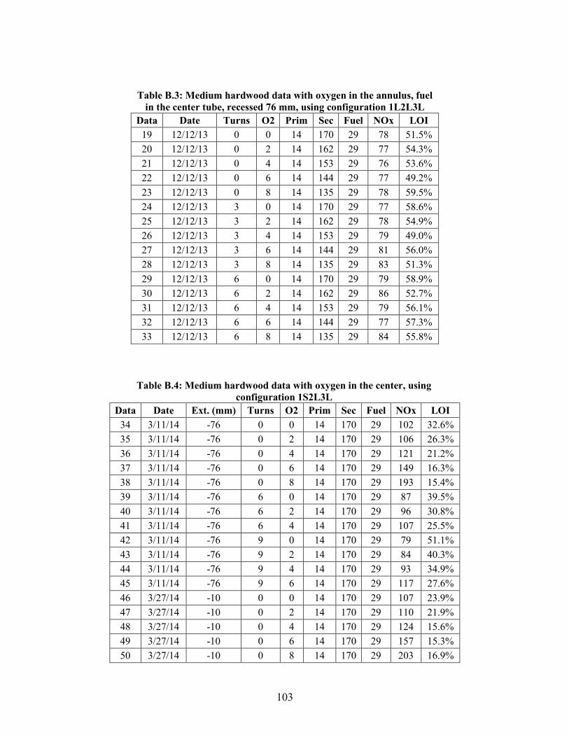
103

Table B.3: Medium hardwood data with oxygen in the annulus, fuel in the center tube, recessed 76 mm, using configuration 1L2L3L

Data Date Turns O2 Prim Sec Fuel NOx LOI 19 12/12/13 0 0 14 170 29 78 51.5% 20 12/12/13 0 2 14 162 29 77 54.3% 21 12/12/13 0 4 14 153 29 76 53.6% 22 12/12/13 0 6 14 144 29 77 49.2% 23 12/12/13 0 8 14 135 29 78 59.5% 24 12/12/13 3 0 14 170 29 77 58.6% 25 12/12/13 3 2 14 162 29 78 54.9% 26 12/12/13 3 4 14 153 29 79 49.0% 27 12/12/13 3 6 14 144 29 81 56.0% 28 12/12/13 3 8 14 135 29 83 51.3% 29 12/12/13 6 0 14 170 29 79 58.9% 30 12/12/13 6 2 14 162 29 86 52.7% 31 12/12/13 6 4 14 153 29 79 56.1% 32 12/12/13 6 6 14 144 29 77 57.3% 33 12/12/13 6 8 14 135 29 84 55.8%

Table B.4: Medium hardwood data with oxygen in the center, using configuration 1S2L3L

Data Date Ext. (mm) Turns O2 Prim Sec Fuel NOx LOI 34 3/11/14 -76 0 0 14 170 29 102 32.6% 35 3/11/14 -76 0 2 14 170 29 106 26.3% 36 3/11/14 -76 0 4 14 170 29 121 21.2% 37 3/11/14 -76 0 6 14 170 29 149 16.3% 38 3/11/14 -76 0 8 14 170 29 193 15.4% 39 3/11/14 -76 6 0 14 170 29 87 39.5% 40 3/11/14 -76 6 2 14 170 29 96 30.8% 41 3/11/14 -76 6 4 14 170 29 107 25.5% 42 3/11/14 -76 9 0 14 170 29 79 51.1% 43 3/11/14 -76 9 2 14 170 29 84 40.3% 44 3/11/14 -76 9 4 14 170 29 93 34.9% 45 3/11/14 -76 9 6 14 170 29 117 27.6% 46 3/27/14 -10 0 0 14 170 29 107 23.9% 47 3/27/14 -10 0 2 14 170 29 110 21.9% 48 3/27/14 -10 0 4 14 170 29 124 15.6% 49 3/27/14 -10 0 6 14 170 29 157 15.3% 50 3/27/14 -10 0 8 14 170 29 203 16.9%

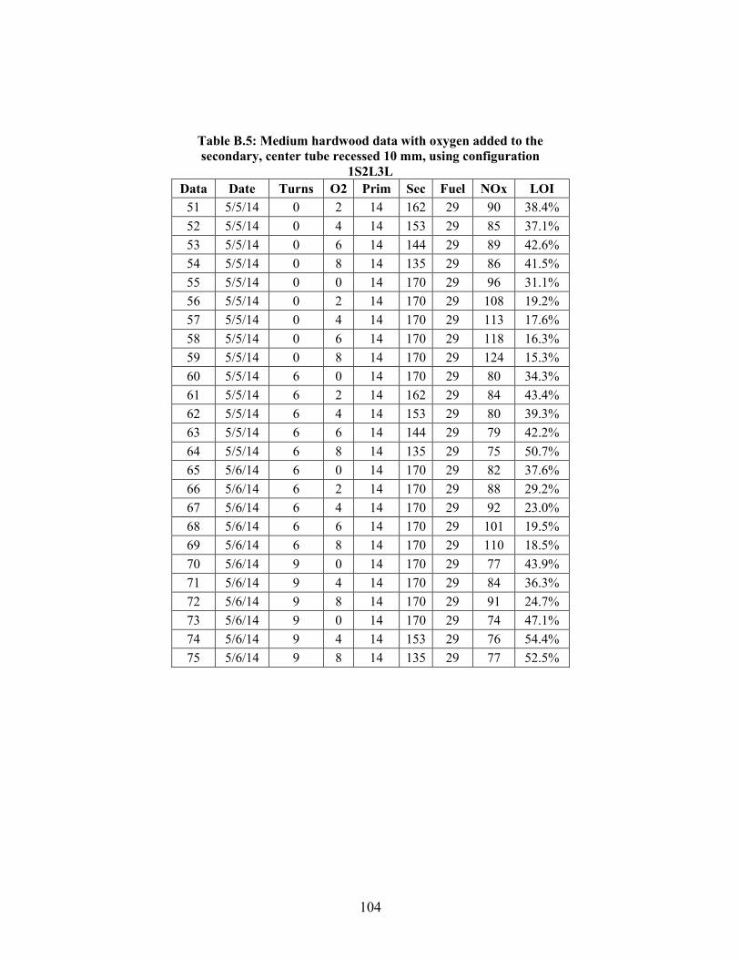
104

Table B.5: Medium hardwood data with oxygen added to the secondary, center tube recessed 10 mm, using configuration

1S2L3L Data Date Turns O2 Prim Sec Fuel NOx LOI

51 5/5/14 0 2 14 162 29 90 38.4% 52 5/5/14 0 4 14 153 29 85 37.1% 53 5/5/14 0 6 14 144 29 89 42.6% 54 5/5/14 0 8 14 135 29 86 41.5% 55 5/5/14 0 0 14 170 29 96 31.1% 56 5/5/14 0 2 14 170 29 108 19.2% 57 5/5/14 0 4 14 170 29 113 17.6% 58 5/5/14 0 6 14 170 29 118 16.3% 59 5/5/14 0 8 14 170 29 124 15.3% 60 5/5/14 6 0 14 170 29 80 34.3% 61 5/5/14 6 2 14 162 29 84 43.4% 62 5/5/14 6 4 14 153 29 80 39.3% 63 5/5/14 6 6 14 144 29 79 42.2% 64 5/5/14 6 8 14 135 29 75 50.7% 65 5/6/14 6 0 14 170 29 82 37.6% 66 5/6/14 6 2 14 170 29 88 29.2% 67 5/6/14 6 4 14 170 29 92 23.0% 68 5/6/14 6 6 14 170 29 101 19.5% 69 5/6/14 6 8 14 170 29 110 18.5% 70 5/6/14 9 0 14 170 29 77 43.9% 71 5/6/14 9 4 14 170 29 84 36.3% 72 5/6/14 9 8 14 170 29 91 24.7% 73 5/6/14 9 0 14 170 29 74 47.1% 74 5/6/14 9 4 14 153 29 76 54.4% 75 5/6/14 9 8 14 135 29 77 52.5%

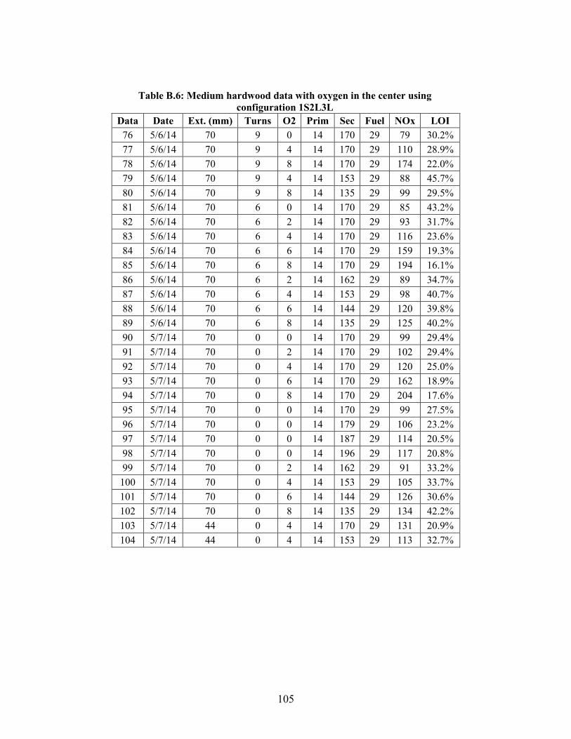
105

Table B.6: Medium hardwood data with oxygen in the center using configuration 1S2L3L

Data Date Ext. (mm) Turns O2 Prim Sec Fuel NOx LOI 76 5/6/14 70 9 0 14 170 29 79 30.2% 77 5/6/14 70 9 4 14 170 29 110 28.9% 78 5/6/14 70 9 8 14 170 29 174 22.0% 79 5/6/14 70 9 4 14 153 29 88 45.7% 80 5/6/14 70 9 8 14 135 29 99 29.5% 81 5/6/14 70 6 0 14 170 29 85 43.2% 82 5/6/14 70 6 2 14 170 29 93 31.7% 83 5/6/14 70 6 4 14 170 29 116 23.6% 84 5/6/14 70 6 6 14 170 29 159 19.3% 85 5/6/14 70 6 8 14 170 29 194 16.1% 86 5/6/14 70 6 2 14 162 29 89 34.7% 87 5/6/14 70 6 4 14 153 29 98 40.7% 88 5/6/14 70 6 6 14 144 29 120 39.8% 89 5/6/14 70 6 8 14 135 29 125 40.2% 90 5/7/14 70 0 0 14 170 29 99 29.4% 91 5/7/14 70 0 2 14 170 29 102 29.4% 92 5/7/14 70 0 4 14 170 29 120 25.0% 93 5/7/14 70 0 6 14 170 29 162 18.9% 94 5/7/14 70 0 8 14 170 29 204 17.6% 95 5/7/14 70 0 0 14 170 29 99 27.5% 96 5/7/14 70 0 0 14 179 29 106 23.2% 97 5/7/14 70 0 0 14 187 29 114 20.5% 98 5/7/14 70 0 0 14 196 29 117 20.8% 99 5/7/14 70 0 2 14 162 29 91 33.2%

100 5/7/14 70 0 4 14 153 29 105 33.7% 101 5/7/14 70 0 6 14 144 29 126 30.6% 102 5/7/14 70 0 8 14 135 29 134 42.2% 103 5/7/14 44 0 4 14 170 29 131 20.9% 104 5/7/14 44 0 4 14 153 29 113 32.7%

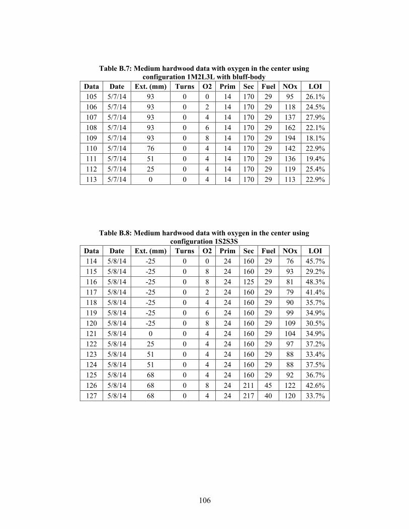
106

Table B.7: Medium hardwood data with oxygen in the center using configuration 1M2L3L with bluff-body

Data Date Ext. (mm) Turns O2 Prim Sec Fuel NOx LOI 105 5/7/14 93 0 0 14 170 29 95 26.1% 106 5/7/14 93 0 2 14 170 29 118 24.5% 107 5/7/14 93 0 4 14 170 29 137 27.9% 108 5/7/14 93 0 6 14 170 29 162 22.1% 109 5/7/14 93 0 8 14 170 29 194 18.1% 110 5/7/14 76 0 4 14 170 29 142 22.9% 111 5/7/14 51 0 4 14 170 29 136 19.4% 112 5/7/14 25 0 4 14 170 29 119 25.4% 113 5/7/14 0 0 4 14 170 29 113 22.9%

Table B.8: Medium hardwood data with oxygen in the center using configuration 1S2S3S

Data Date Ext. (mm) Turns O2 Prim Sec Fuel NOx LOI 114 5/8/14 -25 0 0 24 160 29 76 45.7% 115 5/8/14 -25 0 8 24 160 29 93 29.2% 116 5/8/14 -25 0 8 24 125 29 81 48.3% 117 5/8/14 -25 0 2 24 160 29 79 41.4% 118 5/8/14 -25 0 4 24 160 29 90 35.7% 119 5/8/14 -25 0 6 24 160 29 99 34.9% 120 5/8/14 -25 0 8 24 160 29 109 30.5% 121 5/8/14 0 0 4 24 160 29 104 34.9% 122 5/8/14 25 0 4 24 160 29 97 37.2% 123 5/8/14 51 0 4 24 160 29 88 33.4% 124 5/8/14 51 0 4 24 160 29 88 37.5% 125 5/8/14 68 0 4 24 160 29 92 36.7% 126 5/8/14 68 0 8 24 211 45 122 42.6% 127 5/8/14 68 0 4 24 217 40 120 33.7%

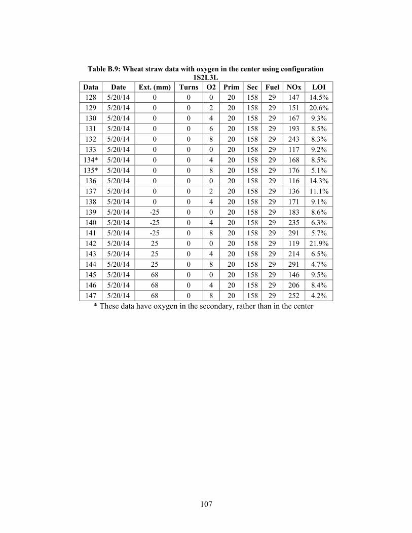
107

Table B.9: Wheat straw data with oxygen in the center using configuration 1S2L3L

Data Date Ext. (mm) Turns O2 Prim Sec Fuel NOx LOI 128 5/20/14 0 0 0 20 158 29 147 14.5% 129 5/20/14 0 0 2 20 158 29 151 20.6% 130 5/20/14 0 0 4 20 158 29 167 9.3% 131 5/20/14 0 0 6 20 158 29 193 8.5% 132 5/20/14 0 0 8 20 158 29 243 8.3% 133 5/20/14 0 0 0 20 158 29 117 9.2% 134* 5/20/14 0 0 4 20 158 29 168 8.5% 135* 5/20/14 0 0 8 20 158 29 176 5.1% 136 5/20/14 0 0 0 20 158 29 116 14.3% 137 5/20/14 0 0 2 20 158 29 136 11.1% 138 5/20/14 0 0 4 20 158 29 171 9.1% 139 5/20/14 -25 0 0 20 158 29 183 8.6% 140 5/20/14 -25 0 4 20 158 29 235 6.3% 141 5/20/14 -25 0 8 20 158 29 291 5.7% 142 5/20/14 25 0 0 20 158 29 119 21.9% 143 5/20/14 25 0 4 20 158 29 214 6.5% 144 5/20/14 25 0 8 20 158 29 291 4.7% 145 5/20/14 68 0 0 20 158 29 146 9.5% 146 5/20/14 68 0 4 20 158 29 206 8.4% 147 5/20/14 68 0 8 20 158 29 252 4.2%

* These data have oxygen in the secondary, rather than in the center

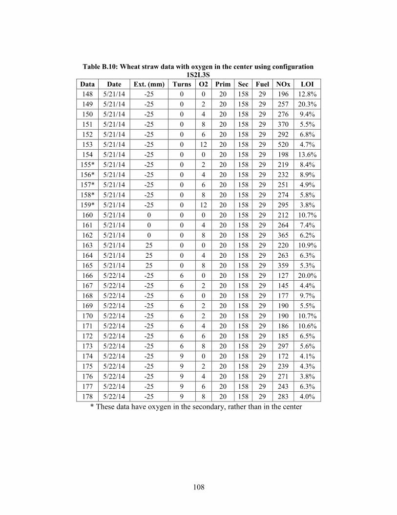
108

Table B.10: Wheat straw data with oxygen in the center using configuration 1S2L3S

Data Date Ext. (mm) Turns O2 Prim Sec Fuel NOx LOI 148 5/21/14 -25 0 0 20 158 29 196 12.8% 149 5/21/14 -25 0 2 20 158 29 257 20.3% 150 5/21/14 -25 0 4 20 158 29 276 9.4% 151 5/21/14 -25 0 8 20 158 29 370 5.5% 152 5/21/14 -25 0 6 20 158 29 292 6.8% 153 5/21/14 -25 0 12 20 158 29 520 4.7% 154 5/21/14 -25 0 0 20 158 29 198 13.6% 155* 5/21/14 -25 0 2 20 158 29 219 8.4% 156* 5/21/14 -25 0 4 20 158 29 232 8.9% 157* 5/21/14 -25 0 6 20 158 29 251 4.9% 158* 5/21/14 -25 0 8 20 158 29 274 5.8% 159* 5/21/14 -25 0 12 20 158 29 295 3.8% 160 5/21/14 0 0 0 20 158 29 212 10.7% 161 5/21/14 0 0 4 20 158 29 264 7.4% 162 5/21/14 0 0 8 20 158 29 365 6.2% 163 5/21/14 25 0 0 20 158 29 220 10.9% 164 5/21/14 25 0 4 20 158 29 263 6.3% 165 5/21/14 25 0 8 20 158 29 359 5.3% 166 5/22/14 -25 6 0 20 158 29 127 20.0% 167 5/22/14 -25 6 2 20 158 29 145 4.4% 168 5/22/14 -25 6 0 20 158 29 177 9.7% 169 5/22/14 -25 6 2 20 158 29 190 5.5% 170 5/22/14 -25 6 2 20 158 29 190 10.7% 171 5/22/14 -25 6 4 20 158 29 186 10.6% 172 5/22/14 -25 6 6 20 158 29 185 6.5% 173 5/22/14 -25 6 8 20 158 29 297 5.6% 174 5/22/14 -25 9 0 20 158 29 172 4.1% 175 5/22/14 -25 9 2 20 158 29 239 4.3% 176 5/22/14 -25 9 4 20 158 29 271 3.8% 177 5/22/14 -25 9 6 20 158 29 243 6.3% 178 5/22/14 -25 9 8 20 158 29 283 4.0%

* These data have oxygen in the secondary, rather than in the center

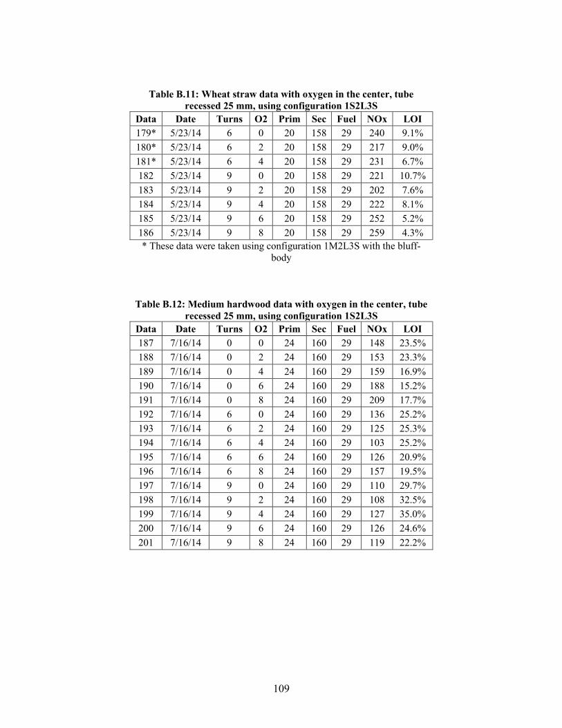
109

Table B.11: Wheat straw data with oxygen in the center, tube recessed 25 mm, using configuration 1S2L3S

Data Date Turns O2 Prim Sec Fuel NOx LOI 179* 5/23/14 6 0 20 158 29 240 9.1% 180* 5/23/14 6 2 20 158 29 217 9.0% 181* 5/23/14 6 4 20 158 29 231 6.7% 182 5/23/14 9 0 20 158 29 221 10.7% 183 5/23/14 9 2 20 158 29 202 7.6% 184 5/23/14 9 4 20 158 29 222 8.1% 185 5/23/14 9 6 20 158 29 252 5.2% 186 5/23/14 9 8 20 158 29 259 4.3% * These data were taken using configuration 1M2L3S with the bluff-

body

Table B.12: Medium hardwood data with oxygen in the center, tube recessed 25 mm, using configuration 1S2L3S


110

Table B.13: Hardwood data under over-fire air conditions, 52 kg/hr tertiary air, oxygen in the center, center tube flush, using

configuration 1S2L3L Data Date Turns O2 Prim Sec Fuel NOx LOI 202 10/29/14 0 0 14 118 29 107 25.8% 203 10/29/14 0 4 14 118 29 109 23.3% 204 10/29/14 0 6 14 118 29 124 19.7% 205 10/29/14 0 8 14 118 29 142 18.4% 206 10/29/14 0 0 14 118 29 108 29.3% 207 10/29/14 0 2 14 110 29 110 28.1% 208 10/29/14 0 4 14 101 29 114 27.2% 209 10/29/14 0 6 14 92 29 130 27.6% 210 10/29/14 0 8 14 83 29 135 24.5%

Table B.14: Medium hardwood data with oxygen in the center, center tube flush, using configuration 1L2L3L


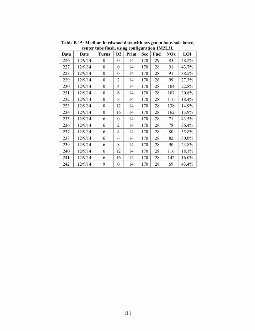
111

Table B.15: Medium hardwood data with oxygen in four-hole lance, center tube flush, using configuration 1M2L3L

Data Date Turns O2 Prim Sec Fuel NOx LOI 226 12/9/14 0 0 14 170 29 83 48.2% 227 12/9/14 0 0 14 170 28 91 43.7% 228 12/9/14 0 0 14 170 28 91 38.5% 229 12/9/14 0 2 14 170 28 99 27.3% 230 12/9/14 0 4 14 170 28 104 22.8% 231 12/9/14 0 6 14 170 28 107 20.8% 232 12/9/14 0 8 14 170 28 116 18.4% 233 12/9/14 0 12 14 170 28 138 14.9% 234 12/9/14 0 16 14 170 28 162 13.9% 235 12/9/14 6 0 14 170 28 71 43.5% 236 12/9/14 6 2 14 170 28 78 36.4% 237 12/9/14 6 4 14 170 28 80 35.8% 238 12/9/14 6 6 14 170 28 82 30.0% 239 12/9/14 6 8 14 170 28 90 23.8% 240 12/9/14 6 12 14 170 28 116 18.1% 241 12/9/14 6 16 14 170 28 142 16.0% 242 12/9/14 9 0 14 170 28 69 43.4%

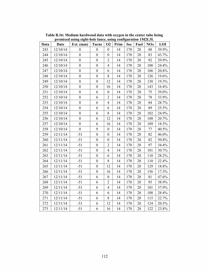
112

Table B.16: Medium hardwood data with oxygen in the center tube being premixed using eight-hole lance, using configuration 1M2L3L

Data Date Ext. (mm) Turns O2 Prim Sec Fuel NOx LOI 243 12/10/14 0 0 0 14 170 28 88 39.9% 244 12/10/14 0 0 0 14 170 28 83 43.7% 245 12/10/14 0 0 2 14 170 28 92 29.9% 246 12/10/14 0 0 4 14 170 28 100 24.4% 247 12/10/14 0 0 6 14 170 28 106 20.8% 248 12/10/14 0 0 8 14 170 28 126 19.6% 249 12/10/14 0 0 12 14 170 28 130 19.3% 250 12/10/14 0 0 16 14 170 28 143 16.4% 251 12/10/14 0 6 0 14 170 28 75 39.0% 252 12/10/14 0 6 2 14 170 28 78 33.9% 253 12/10/14 0 6 4 14 170 28 84 28.7% 254 12/10/14 0 6 6 14 170 28 89 25.5% 255 12/10/14 0 6 8 14 170 28 102 24.9% 256 12/10/14 0 6 12 14 170 28 108 20.7% 257 12/10/14 0 6 16 14 170 28 109 18.5% 258 12/10/14 0 9 0 14 170 28 77 40.5% 259 12/11/14 -51 0 0 14 170 28 82 46.0% 260 12/11/14 -51 0 0 14 170 28 82 50.8% 261 12/11/14 -51 0 2 14 170 28 97 34.4% 262 12/11/14 -51 0 4 14 170 28 101 30.7% 263 12/11/14 -51 0 6 14 170 28 110 28.2% 264 12/11/14 -51 0 8 14 170 28 110 22.4% 265 12/11/14 -51 0 12 14 170 28 129 18.8% 266 12/11/14 -51 0 16 14 170 28 156 17.3% 267 12/11/14 -51 6 0 14 170 28 81 47.6% 268 12/11/14 -51 6 2 14 170 28 95 38.9% 269 12/11/14 -51 6 4 14 170 28 101 37.9% 270 12/11/14 -51 6 6 14 170 28 108 28.4% 271 12/11/14 -51 6 8 14 170 28 115 22.7% 272 12/11/14 -51 6 12 14 170 28 124 20.5% 273 12/11/14 -51 6 16 14 170 28 122 23.8%

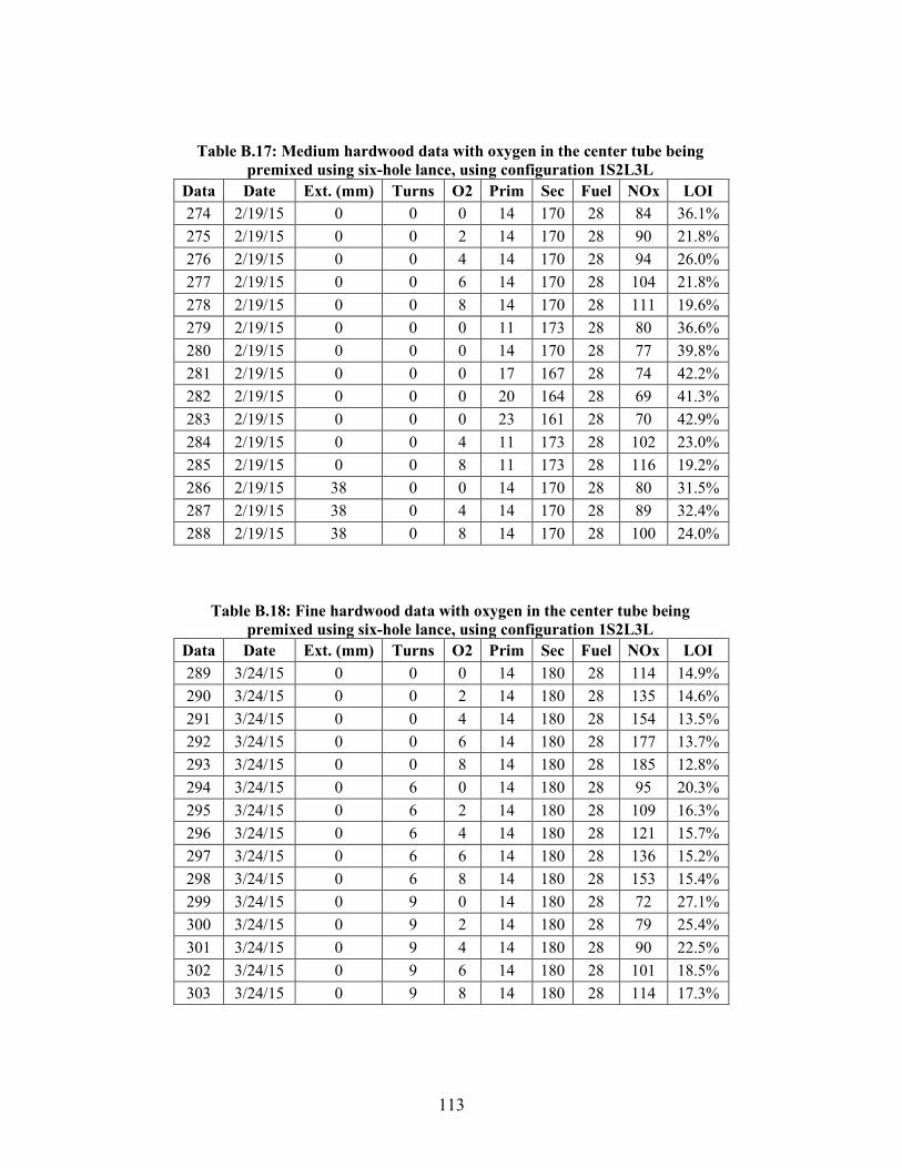
113

Table B.17: Medium hardwood data with oxygen in the center tube being premixed using six-hole lance, using configuration 1S2L3L

Data Date Ext. (mm) Turns O2 Prim Sec Fuel NOx LOI 274 2/19/15 0 0 0 14 170 28 84 36.1% 275 2/19/15 0 0 2 14 170 28 90 21.8% 276 2/19/15 0 0 4 14 170 28 94 26.0% 277 2/19/15 0 0 6 14 170 28 104 21.8% 278 2/19/15 0 0 8 14 170 28 111 19.6% 279 2/19/15 0 0 0 11 173 28 80 36.6% 280 2/19/15 0 0 0 14 170 28 77 39.8% 281 2/19/15 0 0 0 17 167 28 74 42.2% 282 2/19/15 0 0 0 20 164 28 69 41.3% 283 2/19/15 0 0 0 23 161 28 70 42.9% 284 2/19/15 0 0 4 11 173 28 102 23.0% 285 2/19/15 0 0 8 11 173 28 116 19.2% 286 2/19/15 38 0 0 14 170 28 80 31.5% 287 2/19/15 38 0 4 14 170 28 89 32.4% 288 2/19/15 38 0 8 14 170 28 100 24.0%

Table B.18: Fine hardwood data with oxygen in the center tube being premixed using six-hole lance, using configuration 1S2L3L

Data Date Ext. (mm) Turns O2 Prim Sec Fuel NOx LOI 289 3/24/15 0 0 0 14 180 28 114 14.9% 290 3/24/15 0 0 2 14 180 28 135 14.6% 291 3/24/15 0 0 4 14 180 28 154 13.5% 292 3/24/15 0 0 6 14 180 28 177 13.7% 293 3/24/15 0 0 8 14 180 28 185 12.8% 294 3/24/15 0 6 0 14 180 28 95 20.3% 295 3/24/15 0 6 2 14 180 28 109 16.3% 296 3/24/15 0 6 4 14 180 28 121 15.7% 297 3/24/15 0 6 6 14 180 28 136 15.2% 298 3/24/15 0 6 8 14 180 28 153 15.4% 299 3/24/15 0 9 0 14 180 28 72 27.1% 300 3/24/15 0 9 2 14 180 28 79 25.4% 301 3/24/15 0 9 4 14 180 28 90 22.5% 302 3/24/15 0 9 6 14 180 28 101 18.5% 303 3/24/15 0 9 8 14 180 28 114 17.3%

115

APPENDIX C: FOURIER TRANSFORM INFRARED SPECTROMETER

A Fourier Transform Infrared Spectrometer (FT-IR) is a tool that is used in a variety of

applications, including that of improved gas species mapping within a reactor. The FT-IR can be

used to collect infrared light from an internal source and determine infrared light absorbed by

gases extracted from a reactor. Various gas species have specific bands of light over which they

absorb, which can be detected by the FT-IR. Gases such as NO and CO have small, yet specific

bands where they are known to absorb infrared light. CO2 and H2O, on the other hand, both

absorb over a larger bands. The amount of light absorbed by a gas is dependent on a number of

variables. Gas concentration, gas flow rate, temperature and pressure all play a role in the

amount of light the detector senses. The gas flow rate, temperature, and pressure are held

constant to eliminate variables and to yield gas species concentrations.

Due to the various bands over which different gases absorb, it can be extremely difficult

to differentiate between the various gas species and their concentration. For example, H2O

absorbs over the same wavenumber as NO. Since the baseline has neither of these gas species it

becomes a difficult mathematical challenge. Adding to the difficulty is that NO is in much

smaller quantities and does not absorb light to the level, by an order of magnitude, as does H2O.

A classical least squares (CLS) method can be used to compare various spectra in order to create

a calibration. Once the calibration is made, the FTIR can then display gas species concentration

over a very short time frame. For more theory and general information, see previous work by

Reeder [45] and Chamberlain [46].

116

FT-IR technology has been developed greatly since its first use and it has enormous

potential as a non-intrusive means of analyzing samples. The FT-IR can be an excellent tool in

mapping gas species concentrations within the reactor. The FT-IR connects to a computer to

allow data acquisition through a program named OMNIC. Another program, TQ Analyst, can be

used to create methods for the determination of gas species concentrations and compared with

another software package, MKS, with its own libraries of data. A method acts like a library and

is a collection of spectra. A method allows a comparison of spectra from an unknown gas to the

known gases and calculates the unknown gas based on specified infrared light bands.

A heated pump pulls gas through heated lines from the reactor to a gas cell allowing

infrared absorption levels to be measured using the FT-IR. The absorption levels then allow a gas

concentration within the cell to be calculated using a method created by multiple spectra. A

standard operating procedure for using the gas cell with the FT-IR is shown.

117

Standard Operating Procedure to use FT-IR with Gas Cell

1. Make sure FT-IR and gas cell heater are hooked up properly a. Plug in power cord and white cord from FT-IR to computer b. Plug in thermocouple and power cord into the temperature controller c. Purge FT-IR with N2 to reduce background noise

2. Get Liquid Nitrogen from Central Stockroom (C100 BNSN) a. Approximately 1 liter needed to cool MCT detector b. Use funnel and slowly add liquid nitrogen c. Be careful not to overfill d. It takes about 60 minutes to cool detector

3. Turn on gas cell heater a. Set gas cell heater to run. b. Ensure it is set at 302°F (150°C) c. It will take about 30 minutes to heat up

4. Ensure Pressure Transducer is working properly 5. The gas cell needs to be at 101.325 kPa (1 atm or 760 torr) total pressure when collecting

samples a. Do not overpressure gas cell! b. The maximum pressure it can withstand is 15 psi gauge. c. The gas cell must be at correct total pressure or reading will be inaccurate

6. Collect background with N2 in gas cell a. Make sure N2 is hooked up with the inlet valve to gas cell closed b. Slowly open inlet valve and adjust the inlet valve and flow meter so that the gas

cell is appropriately pressurized c. Flow meter should be about 30 cc/min d. Wait about 3 minutes for other gases to leave gas cell e. Collect background using an appropriate experiment set-up in OMNIC

i. (Suggested settings: Mid IR, N2 Det, 6 Scans, .5cm-1, 5000-500cm-1) f. If there appears to be unusual absorptions in background wait additional time to

ensure N2 is the only gas present in the gas cell and re-collect background g. Once background has been collected turn the three way valve before inlet to

collect sample gases 7. Collect Series with gases you want to sample

a. Open the flow meter valve all the way b. Open the inlet valve to the gas cell c. Turn on the pump and watch the cell pressure d. Adjust valves appropriately to ensure correct cell pressure e. Wait enough time for N2 to leave cell f. Choose “Collect Series…” from the “Collect” drop down menu to begin data

acquisition, be sure to save any desired data g. If needed, repeat step 6 for new background

8. Shut down equipment a. Purge the gas cell with N2 and close valves to prevent corrosion and condensation

in the gas cell b. Turn off all assisting equipment

Burnout, NO, and Flame Characterization from an Oxygen ...

Documents

Transcript of Burnout, NO, and Flame Characterization from an Oxygen ...