Bunker consumption optimization methods in shipping: A ...
39
University of Wollongong University of Wollongong Research Online Research Online Faculty of Engineering and Information Sciences - Papers: Part A Faculty of Engineering and Information Sciences 1-1-2013 Bunker consumption optimization methods in shipping: A critical review Bunker consumption optimization methods in shipping: A critical review and extensions and extensions Shuaian Wang University of Wollongong, [email protected] Qiang Meng National University of Singapore Zhiyuan Liu Monash University Follow this and additional works at: https://ro.uow.edu.au/eispapers Part of the Engineering Commons, and the Science and Technology Studies Commons Recommended Citation Recommended Citation Wang, Shuaian; Meng, Qiang; and Liu, Zhiyuan, "Bunker consumption optimization methods in shipping: A critical review and extensions" (2013). Faculty of Engineering and Information Sciences - Papers: Part A. 1296. https://ro.uow.edu.au/eispapers/1296 Research Online is the open access institutional repository for the University of Wollongong. For further information contact the UOW Library: [email protected]
Transcript of Bunker consumption optimization methods in shipping: A ...

University of Wollongong University of Wollongong
Research Online Research Online
Faculty of Engineering and Information Sciences - Papers: Part A
Faculty of Engineering and Information Sciences
1-1-2013
Bunker consumption optimization methods in shipping: A critical review Bunker consumption optimization methods in shipping: A critical review
and extensions and extensions
Shuaian Wang University of Wollongong, [email protected]
Qiang Meng National University of Singapore
Zhiyuan Liu Monash University
Follow this and additional works at: https://ro.uow.edu.au/eispapers
Part of the Engineering Commons, and the Science and Technology Studies Commons
Recommended Citation Recommended Citation Wang, Shuaian; Meng, Qiang; and Liu, Zhiyuan, "Bunker consumption optimization methods in shipping: A critical review and extensions" (2013). Faculty of Engineering and Information Sciences - Papers: Part A. 1296. https://ro.uow.edu.au/eispapers/1296
Research Online is the open access institutional repository for the University of Wollongong. For further information contact the UOW Library: [email protected]
Bunker consumption optimization methods in shipping: A critical review and Bunker consumption optimization methods in shipping: A critical review and extensions extensions
Abstract Abstract It is crucial nowadays for shipping companies to reduce bunker consumption while maintaining a certain level of shlpping service in view of the high bunker price and concerned shipping emissions. After introducing the three bunker consumption optimization contexts: minimization of total operating cost. minimization of emission and collaborative mechanisms between port operators and shipping companies, this paper presents a aiticaJ and timely literature review on mathematical solution methods for bunker consumption optimization problems. Several navel bunker consumption optimization methods are subsequently proposed. The applicability, optimality, and efficiency of the existing and newly proposed methods are al5o analyzed. This paper provides technical guidelines and insights for researchers and practitioners dealing with the bunker consumption issues.
Keywords Keywords era2015
Disciplines Disciplines Engineering | Science and Technology Studies
Publication Details Publication Details Wang, S., Meng, Q. & Liu, Z. (2013). Bunker consumption optimization methods in shipping: A critical review and extensions. Transportation Research Part E: Logistics and Transportation Review, 53 49-62.
This journal article is available at Research Online: https://ro.uow.edu.au/eispapers/1296

Bunker Consumption Optimization Methods in Shipping: A Critical Review and
Extensions
Shuaian Wanga, Qiang Meng
b∗, Zhiyuan Liu
c
aSchool of Mathematics and Applied Statistics, University of Wollongong, Wollongong, NSW
2522, Australia
bDepartment of Civil and Environmental Engineering, National University of Singapore,
Singapore 117576
cInstitute of Transport Studies, Department of Civil Engineering, Monash University, Clayton,
Victoria 3800, Australia
Abstract
It is crucial nowadays for shipping companies to reduce bunker consumption while
maintaining a certain level of shipping service in view of the high bunker price and
concerned shipping emissions. After introducing the three bunker consumption optimization
contexts: minimization of total operating cost, minimization of emission and collaborative
mechanisms between port operators and shipping companies, this paper presents a critical
and timely literature review on mathematical solution methods for bunker consumption
optimization problems. Several novel bunker consumption optimization methods are
subsequently proposed. The applicability, optimality, and efficiency of the existing and newly
proposed methods are also analyzed. This paper provides technical guidelines and insights for
researchers and practitioners dealing with the bunker consumption issues.
Key Words: Shipping; Sailing speed; Bunker consumption optimization; Mixed-integer
nonlinear programming
∗ Corresponding author, Tel.: +65-6516 5494, Fax: +65-6779 1635
E-mail addresses: [email protected] (S. Wang), [email protected] (Q. Meng),
[email protected] (Z. Liu)

2
1 Introduction
Maritime transportation is the backbone of world trade, and world seaborne trade was
estimated at 8.4 billion tons in terms of the total goods loaded in 2011 (UNCTAD, 2011). In
recent years, increased competition and global shipping downturn have been putting
downward pressure on the revenues of shipping companies; at the same time, increased
security regulations and fuel prices continued to increase their operating costs. The bunker
cost constitutes a large proportion of the operating cost of a shipping company (Notteboom,
2006). For example, Ronen (2011) estimated that when bunker fuel price is around 500 USD
per ton the bunker cost constitutes about three quarters of the operating cost of a large
containership.
The amount of bunker consumed by ships also determines the amount of gas emission,
including Green House Gas (GHG) such as carbon dioxide (CO2), methane (CH4), and
nitrous oxide (N2O), Non-Green House Gases such as sulphur oxides (SOx) and nitrogen
oxides (NOx), and various other pollutants, such as particulate matter, volatile organic
compounds, and black carbon (Psaraftis and Kontovas, 2013). The above gases have negative
effect on global climate. For example, GHGs contribute to global warming, SOx causes acid
rain and deforestation, and NOx causes undesirable health effects. According to the 2009
GHG study by the International Maritime Organization (IMO, 2009), international shipping
contributes 2.7% of the CO2 emitted globally. IMO is currently considering many measures
to reduce GHGs (Psaraftis, 2012). For instance, the IMO Marpol 73/78 Annex VI regulations
aim to reduce nitrogen oxide (NOx) emissions and prevent sulphur oxide (SOx) and

3
particulate matter emissions from ships. In view of strict regulations on CO2 emission,
tradable CO2 emission schemes have been developed and applied, and the current average
contract price is about 8 Euros per ton of CO2 emitted (ICE-ECX, 2012). To meet future
regulation on emission, shipping companies must either reduce bunker consumption or use
cleaner but more expensive bunker fuel, or purchase emission quota from other companies.
1.1 Impact of sailing speed on shipping capacity, inventory cost and bunker
consumption
The bunker consumption of a ship on one hand depends on the design and structure of
the ship, and it is on the other hand very sensitive to the sailing speed. This study focuses on
the impact analysis of sailing speed on bunker consumption.
Fig. 1 plots the relations between sailing speed and bunker consumption for 4 types of
ships: ships with a capacity of 3000 twenty-foot equivalent units (3000-TEU ships for short),
5000-TEU ships, 8000-TEU ships and 10000-TEU ships. Clearly, when the speed increases,
the bunker consumption increases more than linearly. Ronen (1982) mentioned that daily
bunker consumption is approximately proportional to the sailing speed cubed, and Wang and
Meng (2012a) further calibrated the relation using historical operating data of containerships
and found that the exponent is between 2.7 and 3.3, which supports the third power
approximation. Du et al. (2011) used the exponent of 3.5 for feeder containerships, 4 for
medium-sized containerships, and 4.5 for jumbo containerships according to suggestions of a
ship engine manufacturing company. Kontovas and Psaraftis (2011) suggested using an
exponent of 4 or greater when the speed is greater than 20 knots.

4
<Fig 1 is inserted here>
In general, a higher sailing speed has both advantages and disadvantages. The first
advantage is that the amount of cargo that can be shipped annually is larger. For example,
consider a ship with a capacity of 10,000 tons that sails between two ports (A and B) whose
distance is 10000 n miles, and suppose that the total time for discharging and then loading a
full ship load is 3 days at each port, as shown in Fig. 2. If the ship sails at 15 knots, it needs
3+10,000/(24×15)≈30.8 days to transport 10,000 tons of cargo from port A to port B (or from
port B to port A). Therefore in one year it can transport 365/30.8×10,000 = 1.19×10⁶ tons of
cargo. If the ship sails at 20 knots, it needs only 23.8 days to ship cargo from A to B and
hence would be able to transport 1.53×10⁶ tons of cargo annually. The second advantage is
that the inventory cost associated with shipping is lower. In the above example, the cargo
needs a total of 30.8 days for maritime transportation and handling if the ship sails at 15 knots,
and needs only 23.8 days at the speed of 20 knots. The inventory cost of containerized cargos
is high because of the high value of the cargos. For instance, Notteboom (2006) estimated
that one day delay of a 4, 000-TEU ship implies a total cost of 57, 000 Euros associated with
the cargos in the containers; Bakshi and Gans (2010) estimated the inventory cost of
containerized cargo at 0.5 per cent the value of a container per day.
The disadvantage of a higher sailing speed is that the amount of bunker burned is much
higher. Suppose that the daily bunker consumption is proportional to the sailing speed cubed.
As a result, the bunker consumption for accomplishing a trip from port A to port B in Fig. 2 is
proportional to the sailing speed squared (the daily bunker consumption is proportional to the
sailing speed cubed, but the number of days required is inversely proportional to the sailing

5
speed). Therefore, the amount of bunker consumed annually at the speed of 20 knots
(proportional to 202×(365/23.8) ≈6134) is 130% higher than that at the speed of 15 knots
(proportional to 152×(365/30.8) ≈2666), and the amount of cargo carried is only (1.53-
1.19)/1.19≈29% higher. Consequently, the optimal sailing speed is desirable to balance the
tradeoffs between cargo shipping capability, inventory cost, and bunker cost.
<Fig 2 is inserted here>
1.2 Contexts of bunker consumption optimization
In literature, bunker consumption optimization is cast into three application contexts. The
first one is minimizing the operating cost of a shipping company by optimizing the sailing
speed. For example, in shipping network design (Alvarez, 2009), ship fleet deployment
(Gelareh and Meng, 2010), ship schedule construction (Qi and Song, 2012; Wang and Meng,
2012b), sailing speed optimization (Norstad et al., 2011; Ronen, 2011; Wang and Meng,
2012a), and selection of bunkering port and volume (Yao et al., 2012). As aforementioned, a
lower speed means larger inventory cost. However, the inventory cost is borne by shippers
and hence is not directly related to the shipping companies. Therefore, inventory cost is not
considered in most of the studies in this category. Some studies explicitly incorporate the
inventory cost (e.g., Wang and Meng, 2011 for schedule design), or impose a certain level of
service in terms of the maximum allowable origin-to-destination (OD) transit time (Meng and
Wang, 2011).
In the second category, the amount of emission (usually converted to CO2 equivalent) is
formulated in the model (Corbett, 2009; Kontovas and Psaraftis, 2011). From the

6
government’s viewpoint, imposing a fuel tax would effectively lower down the sailing speed
of ships, thereby reducing the emissions at least in the short term (Corbett, 2009). From the
shipping company’s viewpoint, taking the minimization of bunker consumption (which is
proportional to emission) as an objective has two implications: one is to fulfill the
international or local regulations on ship emission; the other is to build an image of social
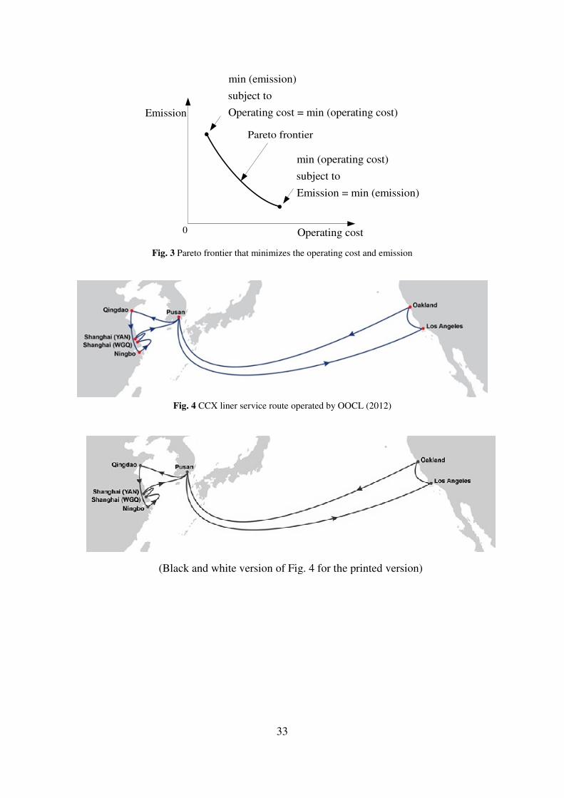
responsibility. To account for emission in modeling, one approach is to minimize the
weighted sum of operating cost and emission. Mathematically, this approach is equivalent to
an increase of bunker price. Another possible approach aims to minimize the operating cost
while ensuring that the emission cannot exceed a certain upper limit. This approach can be
adopted to find Pareto-optimal solutions that minimize the operating cost and emission, as
shown in Fig. 3.
<Fig 3 is inserted here>
In the third category, port operators take into account the bunker cost of the shipping
companies (Golias et al., 2010; Lang and Veenstra, 2010; Du et al., 2011; Wang et al., 2013),
which contrasts conventional planning approaches where port operators maximize their own
efficiency in berth allocation. In such a setting, port operators prioritize the berthing of
incoming ships while accounting for the bunker cost of incoming ships. After that, port
operators inform each ship captain a suggested arrival time, and as a result the ship could
slow down to save bunker if the port is already very congested. For example, suppose that the
ship is 200 n miles away from the port, and it has to wait for 5 hours for a berth if it sails at
its current speed 20 knots. If the port operator informs the ship captain that a berth is
available only 200/20+5=15 hours later, then the captain could slow down to a speed of

7
200/15=13.3 knots, resulting in a significant reduction in bunker consumption. We give
another example with more than one ship. Suppose that there are two identical ships
approaching one port. One ship is sailing at the speed of 20 knots from 1000 n miles away,
and the other is sailing at 25 knots from 1250 n miles away. Both ships need 10 hours’ time
for container handling at berth and both ships desire to be berthed in 60 hours. Only one berth
is available for these two ships. If all other conditions are the same (identical ships sailing
under the same condition and requiring the same container handing operations at the port),
the port operators should let the ship at 20 knots be berthed first, and inform the ship at 25
knots to slow down to the speed of 1250/(1000/20+10)=20.8 knots. Note that if the ship at 25
knots is berthed first, the resulting bunker cost reduction is smaller, because the bunker
consumption is more sensitive to speed when the speed is higher.
1.3 Objectives and contributions
Investigations on the solution methods are of considerable difficulty/significance for the
bunker consumption optimization problems, due to the nonlinearity of bunker consumption
relation with sailing speed and existence of discrete decision variables (the number of ships to
deploy or berth allocation decisions). As a consequence, the objective of this paper is to
critically review the solution methods proposed in the literature and then design efficient
solution methods that supplement the existing methods. Contributions of this paper are
threefold. First, we provide a complete framework on tailored ε-optimal solution methods,
and this framework enables us to design six new tailored ε-optimal solution methods. Second,
based on Du et al. (2011), we introduce an auto-conduction second-order cone programming

8
(SOCP)-transformation procedure that provides the optimal solution. Third, we review the
existing methods in the literature and methods proposed by this paper and then analyze the
advantages and disadvantages of each method. Hopefully, this review could provide
guidelines for researchers and practitioners for optimizing bunker consumption to minimize
operating cost and emission from the viewpoints of both shipping companies and port
operators. Moreover, the approaches may also be applied to optimize sailing speed in settings
with fixed speed (Christiansen et al., 2004; Shintani et al., 2007; Karlaftis et al., 2009;
Gelareh et al., 2010; Bell et al., 2011; Brouer et al., 2011; Reinhardt and Pisinger, 2012).
The remainder of this paper is organized as follows. Section 2 gives a simple bunker
consumption example for us to demonstrate the solution approaches. Section 3 presents two
basic solution methods: enumeration and dynamic programming. Section 4 introduces a
discretization approach. Section 5 proposes a complete framework on tailored ε-optimal
solution methods. Section 6 is dedicated to an exact SOCP approach. A summary of these
methods are provided in Section 7.
2 A simple bunker consumption optimization example
We present a simple speed optimization example that belongs to the first category of
bunker consumption optimization context. Using this simple example we analyze the steps
and properties of each solution method. It should be mentioned that these methods are also
applicable to other bunker consumption optimization contexts.
Consider the Central China Express (CCX) container liner shipping service operated by
OOCL (2012), as shown in Fig. 4. The port rotation of CCX can be coded by its port calling

9
sequence - 1 2, 1N→ → → →L - where the numbers 1 and N denote its first and last ports
of call, respectively. Define : 1, 2 N=I L . Any port on the service can be coded as the first
port of call because the itinerary is a directed loop. Two different ports of call may denote the
same port with different port calling sequences. The voyage between two consecutive ports of
call on the service is referred to as a leg. The thi leg is defined as the voyage from the th
i port
of call to the th( 1)i + port of call when 1, 2, , 1i N= −L and the thN leg is from the th
N port
of call to the 1st port of call. For example, after choosing Qingdao as the first ports of call in
Fig. 4, the CCX service can be coded as follows: 1 (Qingdao) → 2 (Ningbo) → 3
(Shanghai(WGQ)) → 4 (Shanghai(YAN)) → 5 (Pusan) → 6 (Los Angeles) → 7 (Oakland)
→ 8 (Pusan) → 1 (Qingdao).
<Fig 4 is inserted here>
A string of homogeneous ships are deployed on CCX to provide a weekly service
frequency. For example, if the round-trip time is 42 days, then six ships are deployed to
ensure that each port of call is visited once every week. Every port of call is visited on the
same day of each week. Note that a port of call is different from a port in this study. For
example, the port of Pusan in Fig. 4 is visited twice a week, and hence it corresponds to two
ports of call, one of which is after Shanghai(YAN), and the other of which is after Oakland.
The round-trip time consists of port time and sea time. We assume that the time spent at
each port of call i∈I in a round-trip is fixed and denoted by port
it (h). The time at sea
depends on the distance of each voyage leg and the sailing speed. Let i
L be the oceanic
distance (n mile) and i
v (knot) be the speed on leg i . Then the sailing time on leg i is /i i
L v
(h). We assume that ships have a maximum speed maxV that is subject to the mechanical

10
properties of the ships. Assuming that a total of m ships are deployed on CCX, to maintain a
weekly service, we have
port/ 168i i i
i i
L v t m∈ ∈
+ =∑ ∑I I
(1)
where 168 is the number of hours in a week.
Providing a weekly service alone is not sufficient for customer satisfaction. As a
consequence of competition, a maximum allowable transit time from port of call i∈I to port
of call ,j j i∈ ≠I would be set when designing the service. In fact, the sailing speed has a
significant impact on the level of service. For example, if the distance between two ports is
5000 n miles, then the difference in transit time when sailing at 25 knots and 20 knots is 50
hours, which translates to a total cost of 119, 000 Euros associated with the cargos on a 4,
000-TEU ship (Notteboom, 2006). Let ijT (h) represent this maximum allowable transit time.
If there is no container shipped from port of call i to port of call j , then we could simply set
ijT at a very large number. The transit time from port of call i to port of call j , including the
container handling time at these two ports of call, should not exceed ijT .
Eq. (1) further indicates that generally when the sailing speed is higher (higher bunker
consumption), fewer ships are required to maintain a weekly service (lower ship cost), and
vice versa. Therefore an optimal trade-off between bunker cost and ship cost is desirable. As
the bunker consumption function is different on different voyage legs, we denote by ( )i i
g v
(tons/n mile) the bunker consumption per nautical mile at the speed i
v on leg i . If the daily
bunker consumption is proportional to the speed to the power of i
ω , then ( )i i
g v is
proportional to the speed to the power of 1i
ω − . It is reasonable to assume that ( )i i
g v is a
strictly convex and non-decreasing function. It should be mentioned that in reality the relation

11
between speed and bunker consumption ( )i i
g v may change in different trips because of the
uncertain currents, wind, tides and seasonal storms. In fact, the function ( )i i
g v is calibrated
from historical data of different trips. Therefore, when modeling the function ( )i i
g v can be
considered as an average bunker consumption at the speed i
v .
Represent by bunα (USD/ton) the bunker fuel price and let shipc (USD/week) be the fixed
operating cost of a ship on CCX. The bunker consumption optimization (BCO) problem aims
to determine the number of ships m to deploy and the sailing speed i
v on each leg, in order
to minimize the total operating cost while fulfilling the weekly service and transit time
constraints. The BCO problem can be formulated as:
[BCO] bun ship
,(m )in
i
i i iv m
i
L g v c mα∈
+∑I
(2)
subject to:
port/ 168i i i
i i
L v t m∈ ∈
+ =∑ ∑I I
(3)
port
1
/ , , ,k k k ij
i k j i k j
L v t T i j i j≤ ≤ − ≤ ≤
+ ≤ ∈ <∑ ∑ I (4)
port
,1 1 ,1
/ , , ,k k k ij
i k N k j i k N k j
L v t T i j i j≤ ≤ ≤ ≤ − ≤ ≤ ≤ ≤
+ ≤ ∈ >∑ ∑ I (5)
max0 ,iv V i≤ ≤ ∀ ∈ I (6)
m is a positive integer (7)
The objective function (2) minimizes the sum of bunker cost and ship cost. Constraint (3)
imposes the weekly service frequency. Constraints (4)-(5) enforce the transit time
requirement. Note that we assume that ijT is greater than the second term on the left-hand
side of Eqs. (4)-(5) as otherwise there is no solution. Constraint (6) defines the speed range.
We may also impose a minimum speed as in Ronen (2011) to account for engine wear, then
we need to incorporate some slack time at port or at sea to ensure that “=” holds in constraint

12
(3). Whether the minimum speed is equal to 0 or greater than 0 does not affect the solution
method. Constraint (7) defines the number of ships to be a positive integer.
3 Basic optimization methods
[BCO] is a mixed-integer nonlinear programming model with nonlinear terms in its
objective function (2) and constraints (3)-(5). Moreover, constraints (3)-(5) are non-convex.
Therefore it is very difficult to solve [BCO] directly. There are some basic optimization
methods in literature that address special cases of the BCO problem. One method addresses
the problem by assuming that bunker consumption function ( )i i
g v does not change over
different voyage legs and that there is no transit time constraints shown in Eqs. (4)-(5). The
other is a dynamic programming approach which extends the analytical method by relaxing
the assumption of uniform bunker consumption function ( )i i
g v . Other approaches, such as
linear programming by assuming the bunker consumption is linear with speed (Lang and
Veenstra, 2010) and genetic-algorithm (Golias et al., 2010) cannot guarantee optimality; the
gradient descent method (Qi and Song, 2012) is a general solution method. Therefore, these
methods are not elaborated.
3.1 Enumeration method
Corbett et al. (2009) and Ronen (2011) have implicitly made two assumptions about the
BCO problem. First, they assume that that bunker consumption function ( )i i
g v does not
change over different voyage legs. Second, ijT is assumed to be infinite, or in other words,
constraints (4)-(5) are not incorporated. Under these two assumptions, we prove the following
13
two theorems, which are used by Corbett et al. (2009) and Ronen (2011) without a rigorous
proof.
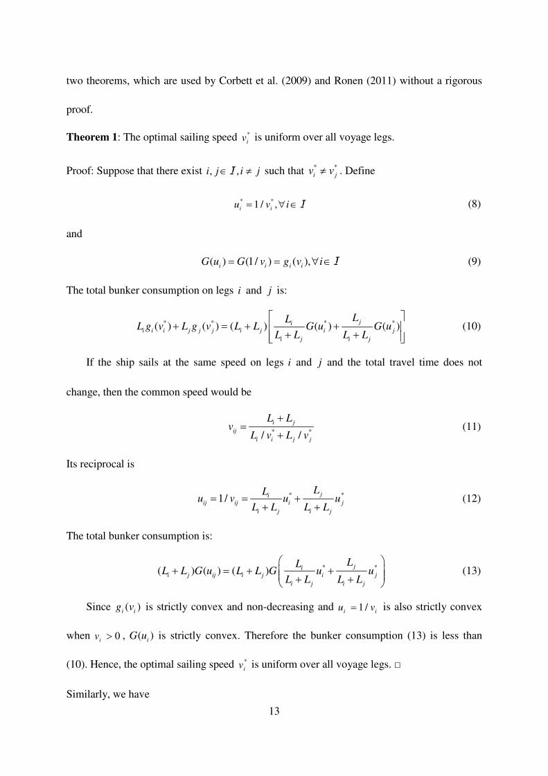
Theorem 1: The optimal sailing speed *
iv is uniform over all voyage legs.
Proof: Suppose that there exist , ,i j i j∈ ≠I such that * *
i jv v≠ . Define
* *1 / ,i iu v i= ∀ ∈ I (8)
and
( ) (1/ ) ( ),i i i i
G u G v g v i= = ∀ ∈I (9)
The total bunker consumption on legs i and j is:
* * * *( ) ( ) ( ) ( ) ( )ji
i i i j j j i j i j
i j i j
LLL g v L g v L L G u G u
L L L L
+ = + +
+ + (10)
If the ship sails at the same speed on legs i and j and the total travel time does not
change, then the common speed would be
* *
/ /
i j
ij
i i j j
L Lv
L v L v
+=
+ (11)
Its reciprocal is
* *1/
ji
ij ij i j
i j i j
LLu v u u
L L L L= = +
+ + (12)
The total bunker consumption is:
* *( ) ( ) ( )ji
i j ij i j i j
i j i j
LLL L G u L L G u u
L L L L
+ = + + + +
(13)
Since ( )i i
g v is strictly convex and non-decreasing and 1 /i iu v= is also strictly convex
when 0iv > , ( )i
G u is strictly convex. Therefore the bunker consumption (13) is less than
(10). Hence, the optimal sailing speed *
iv is uniform over all voyage legs.
Similarly, we have

14
Theorem 2: The optimal sailing speed is constant on each voyage leg.
In view of these two theorems, the BCO problem can be solved easily as it only has two
decision variables: the number of ships m and the common speed denoted by v . The number
of ships m is a positive integer and smaller than e.g. 20 from practical point of view.
Therefore we could enumerate all the possible values of m . For each m we determine the
speed according to Eq. (3) and subsequently calculate the total cost function (2). The optimal
number of ships and the optimal common sailing speed could be determined. Ronen (2011)
employed exactly this procedure and plotted a figure of the change of total operating cost
with the common speed, as shown in Fig. 5. If ( )i i
g v changes over different voyage legs or
ijT is finite, then the optimal speeds on different voyage legs may be different and hence the
above enumeration procedure is no longer applicable.
<Fig 5 is inserted here>
3.2 Dynamic programming method
The dynamic programming (DP) method was applied by Norstad et al. (2011) for solving
a tramp ship routing and scheduling problem. This method is also applicable to the BCO
problem excluding constraints (4)-(5). To implement the dynamic programming method, we
first construct a space-time network where the horizontal axis corresponds to time (time is
discretized into units of e.g. days, 12 hours, 4 hours, or 1 hour, depending on the precision)
and the vertical axis corresponds to the ports of call, as shown in Fig. 6. Note that the
discretization of time corresponds to the discretization of ship speed. For clarity, in Fig. 6 we
assume that the port time port0it = , i∈I . Without loss of generality, the ship visits the first

15
port of call on day 0. An arc from the node (Port 1, Day 0) to a node corresponding to the 2nd
port of call determines the sailing time, speed, and bunker consumption (note that ( )i i
g v
changes over different voyage legs). For example, the arc from (Port 1, Day 0) to (Port 2,
Day 1) corresponds to a much higher bunker cost than the arc from (Port 1, Day 0) to (Port 2,
Day 3) as the former has a much larger sailing speed. Path 1 and Path 2 converge at (Port 3,
Day 6). These two paths have different bunker costs and the same ship cost (or more exactly,
the same trip time from the 1st port of call to the 3
rd one). Evidently, the optimal path in the
space-time network starting from (Port 3, Day 6) relies exclusively on the state (Port 3, Day 6,
and the optimal total bunker cost on leg 1 and leg 2). As a result, only the best path from
(Port 1, Day 0) to (Port 3, Day 6) needs to be recorded when we extend the path to the 4th
, 5th
ports of call, etc. Therefore, a dynamic programming approach is suitable for finding the
optimal number of ships to deploy and the optimal speed *
iv on each voyage leg i∈I .
If ijT is finite, then at each node more information must be recorded. For example, at
(Port 3, Day 6) we also need to record the arrival time at the 2nd
port of call because it affects
the feasibility of the transit time constraint from the 2nd
port of call to other ports of call. As a
consequence, the state of a node contains information on the arrival time at all the previous
ports of call. Therefore, the BCO problem is no longer tractable due to the curse of
dimensionality.
<Fig 6 is inserted here>
16
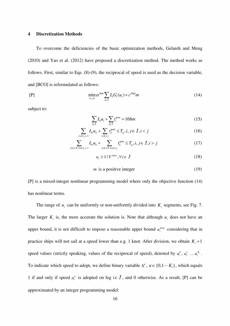
4 Discretization Methods
To overcome the deficiencies of the basic optimization methods, Gelareh and Meng
(2010) and Yao et al. (2012) have proposed a discretization method. The method works as
follows. First, similar to Eqs. (8)-(9), the reciprocal of speed is used as the decision variable,
and [BCO] is reformulated as follows:
[P] bun ship
,(m )in
i
i i iu m
i
LG u c mα∈
+∑I
(14)
subject to:
port 168i i i
i i
L u t m∈ ∈
+ =∑ ∑I I
(15)
port
1
, , ,k k k ij
i k j i k j
L u t T i j i j≤ ≤ − ≤ ≤
+ ≤ ∈ <∑ ∑ I (16)
port
,1 1 ,1
, , ,k k k ij
i k N k j i k N k j
L u t T i j i j≤ ≤ ≤ ≤ − ≤ ≤ ≤ ≤
+ ≤ ∈ >∑ ∑ I (17)
max1 / ,iu V i≥ ∀ ∈ I (18)
m is a positive integer (19)
[P] is a mixed-integer nonlinear programming model where only the objective function (14)
has nonlinear terms.
The range of i
u can be uniformly or non-uniformly divided into i
K segments, see Fig. 7.
The larger i
K is, the more accurate the solution is. Note that although i
u does not have an
upper bound, it is not difficult to impose a reasonable upper bound max
iu considering that in
practice ships will not sail at a speed lower than e.g. 1 knot. After division, we obtain 1i
K +
speed values (strictly speaking, values of the reciprocal of speed), denoted by 0
iu , 1
iu … iK
iu .
To indicate which speed to adopt, we define binary variable ibκ , 0,1
iK∈ Lκ , which equals
1 if and only if speed iuκ is adopted on leg i∈I , and 0 otherwise. As a result, [P] can be
approximated by an integer programming model:
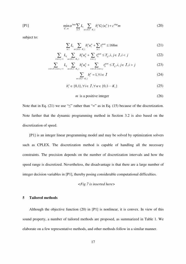
17
[P1] bun ship
,0,1
( )mini
i
i i i ib m
i K
L b G u c mκ
κ κ
κ
α∈ ∈
+∑ ∑LI
(20)
subject to:
port
0,1
168i
i i i i
i K i
L b u t m∈ ∈ ∈
+ ≤∑ ∑ ∑L
κ κ
κI I
(21)
port
1 0,1
, , ,k
k k k k ij
i k j K i k j
L b u t T i j i j≤ ≤ − ∈ ≤ ≤
+ ≤ ∈ <∑ ∑ ∑ I
L
κ κ
κ
(22)
port
,1 1 0,1 ,1
, , ,k
k k k k ij
i k N k j K i k N k j
L b u t T i j i j≤ ≤ ≤ ≤ − ∈ ≤ ≤ ≤ ≤
+ ≤ ∈ >∑ ∑ ∑ I
L
κ κ
κ
(23)
0,1
1,i
i
K
b iκ
κ∈
= ∀ ∈∑ I
L
(24)
0,1, , 0,1 i ib i K∈ ∀ ∈ ∀ ∈I Lκ κ (25)
m is a positive integer (26)
Note that in Eq. (21) we use “≤” rather than “=” as in Eq. (15) because of the discretization.
Note further that the dynamic programming method in Section 3.2 is also based on the
discretization of speed.
[P1] is an integer linear programming model and may be solved by optimization solvers
such as CPLEX. The discretization method is capable of handling all the necessary
constraints. The precision depends on the number of discretization intervals and how the
speed range is discretized. Nevertheless, the disadvantage is that there are a large number of
integer decision variables in [P1], thereby posing considerable computational difficulties.
<Fig 7 is inserted here>
5 Tailored methods
Although the objective function (20) in [P1] is nonlinear, it is convex. In view of this
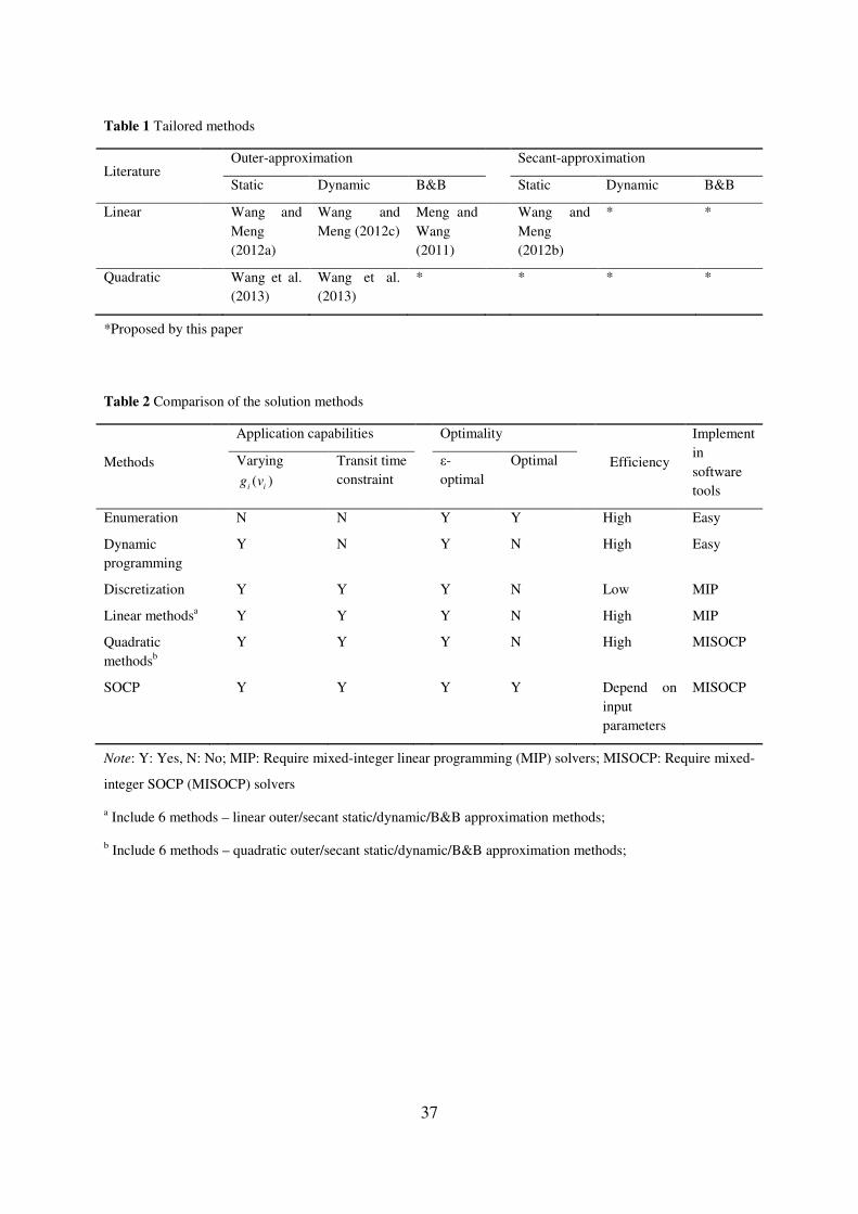
sound property, a number of tailored methods are proposed, as summarized in Table 1. We
elaborate on a few representative methods, and other methods follow in a similar manner.
18
<Table 1 is inserted here>
5.1 Linear static outer-approximation method
In contrast to the discretization method that adds more binary decision variables, the
linear static outer-approximation method adds linear constraints to model [P]. As shown in
Fig. 8 (a), a number of tangent lines are generated, for example, by uniformly dividing i
u , or
uniformly dividing ( )i i
G u , or using as few lines as possible while guaranteeing a maximum
approximation tolerance. The slopes and intercepts of these tangent lines are recorded in a set
iΩ . After introducing auxiliary variables
iG , [P] can be linearized as follows:
[P2] bun ship
, , 0min
i i
i iu m G
i
LG c mα≥
∈
+∑I
(27)
subject to:
slope intercept , , (slope , intercept )i i i i i i iG u iκ κ κ κ≥ × + ∀ ∈ ∀ ∈ΩI (28)
port 168i i i
i i
L u t m∈ ∈
+ =∑ ∑I I
(29)
port
1
, , ,k k k ij
i k j i k j
L u t T i j i j≤ ≤ − ≤ ≤
+ ≤ ∈ <∑ ∑ I (30)
port
,1 1 ,1
, , ,k k k ij
i k N k j i k N k j
L u t T i j i j≤ ≤ ≤ ≤ − ≤ ≤ ≤ ≤
+ ≤ ∈ >∑ ∑ I (31)
max1 / ,iu V i≥ ∀ ∈ I (32)
m is a positive integer (33)
[P2] is a mixed-integer linear programming model. Compared with [P1], the number of
integer decision variables does not increase. Therefore, the computational efficiency of [P2]
is much higher than [P1].
<Fig 8 is inserted here>

19
5.2 Linear dynamic outer-approximation method
The tangent lines can also be generated dynamically whenever necessary, as shown in
Fig. 9. Wang and Meng (2012c) applied the linear dynamic outer-approximation approach in
a slightly different context. The procedure is as follows. First, solve [P2] without constraints
(28). The optimal solution is denoted by * * *( , , , )i i im u G i∈ I . For each leg i∈I , check the gap
between *( )i iG u and *
iG . If this gap is too large, generate a new tangent line at point
* *( , ( ))i i iu G u , add such a constraint to [P2], and resolve. Otherwise, the approximation gap is
acceptable, and the solution is ε-optimal, where ε>0 is a pre-specified tolerance level.
In general, linear dynamic outer-approximation method needs fewer tangent lines than its
static counterpart. However, [P2] has to be solved more than once. Therefore, there is no
straightforward answer whether the dynamic or the static method is preferable.
The static and dynamic methods could also be combined. First, some tangent lines are
generated a priori. Then model [P2] is solved subject to the constraints (28) of these tangent
lines. If the approximation gap is large, generate more tangent lines and resolve. Otherwise
the solution is good enough for practical applications.
<Fig 9 is inserted here>
5.3 Linear branch-and-bound outer-approximation method
The approximation gap can also be narrowed by a branch-and-bound (B&B) scheme.
This method works as follows. First, a few (e.g. 2) tangent lines are generated for each leg,
and model [P2] is solved. The optimal solution is denoted by * * *( , , , )i i im u G i∈ I . If the gap
between *( )i iG u and *
iG is large, then we branch the feasible range of i
u , which is

20
max max[1 / , ]iV u , into two ranges: max *
[1 / , ]iV u and * max[ , ]i iu u . Therefore in one branch,
max *[1 / , ]i iu V u∈ and in the other branch * max
[ , ]i i iu u u∈ . The tangent lines for the original
range max max[1 / , ]iV u are removed and two new tangent lines for the feasible range of
iu in
each branch are generated. Since the width of the ranges of the two new branches is narrower
than the original range, the approximation error on the two new branches should be smaller.
This process is repeated combined with a bounding process, and finally an ε-optimal solution
is obtained.
Meng and Wang (2011) compared the efficiency of the linear B&B outer-approximation
method and the discretization method. Results demonstrate that the former is several orders
more efficient than the latter.
<Fig 10 is inserted here>
5.4 Linear static secant-approximation method
Instead of using tangent lines, we could also use secant lines to approximate the
nonlinear function ( )i i
G u , as shown in Fig. 8 (b). The tangent lines always underestimate
bunker consumption and secant lines may underestimate or overestimate bunker consumption.
Tangent lines seem to be the natural choice of approximation. However, to achieve the same
accuracy, fewer secant lines are needed than tangent lines.
Given an approximation tolerance ε>0 , the secant lines can be generated as follows, as
shown in Fig. 11:
Function Generate Secant Lines min max max
( , ( ), 1/ , )i i i i i
u G u u V u=

21
Define points min min
1 ( , ( ))i i i
A u G u= , max max
1 ( , ( ))i i i
D u G u= , min min
2 ( , ( ) )i i i
A u G u ε= − ,
max max
2 ( , ( ) )i i i
D u G u ε= + .
(a) If the maximum gap between line 2 2A D and the curve ( )i i
G u over the interval
min max[ , ]
i iu u does not exceed ε, as shown in Fig. 11 (a)-(b), then only the line 2 2A D
is generated. Return.
(b) Generate a line that passes point 2A with slope k (the value of k is to be
determined). The line is:
min min( ) ( )i i i i iG k u u G u ε= − + − (34)
Let *
iu be the point corresponding to the maximum difference of the line and the
curve ( )i i
G u over the interval min max
[ , ]i i
u u , that is,
* min max min min: arg max [ , ] | ( ) ( ) ( )i i i i i i i i i iu u u u k u u G u G uε= ∈ − + − − (35)
The value of k is chosen such that the maximum gap is equal to ε, that is,
* min min *( ) ( ) ( )i i i i i ik u u G u G uε ε− + − − = (36)
as shown in Fig. 11 (c), where the point * *
1 ( , ( ))i i i
B u G u= , and point
* *
2 ( , ( ) )i i i
B u G u ε= + . Apparently,
min * max
i i iu u u< < (37)
(b.1) If the gap between the curve ( )i i
G u and the line at max
i iu u= is not greater
than ε, as shown in Fig. 11 (c). The line is sufficient to ensure ε-optimality.
Return.
(b.2) Record the generated line and find the value of min -new
i iu u= such that the
difference of the curve ( )i i
G u and the line at min -new
i iu u= is equal to ε, as shown

22
in Fig. 11 (d). Call the function Generate Secant Lines min -new max
( , ( ), , )i i i i i
u G u u u .
Return.
<Fig 11 is inserted here>
5.5 Quadratic static outer-approximation method
Instead of using straight lines, we could also use parabolic curves to approximate the
nonlinear function ( )i i
G u , as shown in Fig. 8 (c). A parabola can be defined by three
parameters a , b , ci i i
κ κ κ . Let parabola
iΩ be a set representing the parameters a , b , ci i i
κ κ κ of the
parabolas). Eq. (28) can be replaced with:
2 parabolaa ( ) b c , , (a , b , c )i i i i i i i i i iG u u iκ κ κ κ κ κ≥ × + × + ∀ ∈ ∀ ∈ΩI (38)
Evidently, a 0i >κ and therefore Eq. (38) can be transformed to second-order cone
programming (SOCP) constraints. A simple SOCP constraint has the form
2 2
2|| , || , that is, x y z x y z≤ + ≤ (39)
A frequently encountered form 2x yz≤ , , , 0x y z ≥ can also be transformed to SOCP
constraint
2|| , ( ) / 2 || ( ) / 2x y z y z− ≤ + (40)
Optimization solvers such as CPLEX could solve mixed-integer SOCP models. How to
generate the parabolic curves and how to transform Eq. (38) to SOCP constraints are
elaborated in Wang et al. (2013).
A parabola outperforms a straight line in approximating the nonlinear function ( )i i
G u
because a straight line can be considered an extreme case of a parabola when a 0i =κ .
However, solving a model with an SOCP constraint is more time-consuming than a linear
23
constraint. Therefore it is not easy to say whether straight lines or parabolic curves are
preferable.
6 An exact second-order cone programming approach
The function ( )i i
G u is generally assumed or calibrated to be a power function in most
studies. If the daily bunker consumption is proportional to the thi
ω power of the speed,
defining 1-i i=ρ ω , then ( )
i iG u can be represented by:
1( ) ( ) ( ) ,i i
i i i i i iG u u u iω ρβ β−= = ∀ ∈ I (41)
where i
β is a parameter calibrated from historical data. After introducing intermediate
variables i
h , the objective function (27) and constraint (28) in [P2] can be replaced by
[P3] bun ship
, , 0min
i i
i i iu m h
i
L h c mα β≥
∈
+∑I
(42)
( ) ,i
i ih u iρ≥ ∀ ∈ I (43)
To simplify the notation, we suppress the subscript i in Eq. (43) in the sequel. Du et al.
(2011) showed that when 3.5, 4.0, 4.5∈ω , constraint (43) can be transformed (NOT
approximated) to SOCP constraints. For example, when 3=ω , the constraint 2h u
−≥ is
equivalent to two SOCP constraints by introducing an intermediate variable s :
2 2 21 , , that is, 1 , su s h su s h≤ ≤ ≤ ≤ (44)
As a result, [P3] can be transformed to a mixed-integer SOCP model and solved by CPLEX.
The seminal work by Du et al. (2011) pointed out that a more general constraint h u≥ ρ
can be transformed to SOCP constraints. However, this work did not mention how to
implement such a transformation. In this paper we introduce an auto-conduction SOCP-
transformation procedure. To this end, we rewrite it as:
24
1- 11h u h u h uρ ρ ω ω= −≥ ⇔ ≥ ⇔ ≤ (45)
We can state 1ω − as the quotient of two positive integers 1n and 2n :
2
1
1n
nω − = (46)
Hence, Eq. (45) is:
2
11
n
nh u≤ (47)
or
1 21n n
h u≤ (48)
Define
1 2: arg min is an integer | 2 n n
κκ κ= ≥ +%% (49)
Eq. (47) can be transformed to:
1 2 1 2221 1n n n n
h uκκ − −≤ (50)
We examine a general case of Eq. (50) and transform it to SOCP constraints. The general
case we consider is:
31 22
1 2s h u s≤κ θθ θ
(51)
where 1 2, , ,s h u s are nonnegative variables, 1 2 3, , ,θ θ θ κ are nonnegative integers, and
1 2 3 2+ + = κθ θ θ (52)
Evidently, if we can transform Eq. (51) to SOCP constraints, we can also transform Eq. (50)
to SOCP constraints by adding linear constraints 1 1s = and 2 1s = . Without loss of generality,
we define that 1 2 3≥ ≥θ θ θ . In other words, whenever we call the repetitive SOCP
Transformation function below, we should ensure that:
1 2 3≥ ≥θ θ θ (53)
Function SOCP Transformation 1 2 1 2 3( , , , , , , , )s h u s κ θ θ θ

25
(a) If 1=κ , then there are only two possible scenarios: 1 2 32, 0= = =θ θ θ or
1 2 31, 0= = =θ θ θ . (a.1) If 1 2 32, 0= = =θ θ θ , constraint (51) is equivalent to:
1s h≤ (54)
(a.2) Else we have 1 2 31, 0= = =θ θ θ and thus constraint (51) is equivalent to:
2
1s hu≤ (55)
Return.
(b) Else if all 1 2 3, ,θ θ θ are even and 2≥κ , we can divide each of 1 2 3, ,θ θ θ by 2, and
set 1← −κ κ . Call SOCP Transformation 1 2 1 2 3( , , , , 1, / 2, / 2, / 2)s h u s −κ θ θ θ ,
return.
(c) Else there are two possible scenarios: (c.1) 1
1 2−≥ κθ and (c.2)
1
1 1 2 3max( , , ) 2−= < κθ θ θ θ .
(c.1) If 1
1 2−≥ κθ , after introducing intermediate nonnegative variable 3s , Eq. (51) is
transformed to:
11 1 1 1 1
31 222 2 2 2 2 2
1 3 3 2 and s s h s h h h u s−− − − − − −≤ ≤
κκ κ κ κ κ κ θθ θ (56)
or,
11
31 222 2
1 3 3 2 and s s h s h u s−− −≤ ≤
κκ θθ θ (57)
The first constraint in Eq. (57) is already an SOCP constraint. To transform the
second constraint in Eq. (57) and impose the condition in Eq. (53), there are three
scenarios. (c.1.1) If 1
1 22−− ≥κθ θ , call SOCP Transformation
1
3 2 1 2 3( , , , , 1, 2 , , )s h u s−− − κκ θ θ θ ; (c.1.2) else if 1
1 32−− <κθ θ , call SOCP
Transformation 1
3 2 2 3 1( , , , , 1, , , 2 )s u s h−− − κκ θ θ θ ; (c.1.3) else call SOCP
Transformation 1
3 2 2 1 3( , , , , 1, , 2 , )s u h s−− − κκ θ θ θ . Return.
26
(c.2) Else we have 1
1 1 2 3max( , , ) 2−= < κθ θ θ θ . Hence 1
3 2−< κθ . As
1 2 3 2+ + = κθ θ θ , we
have 1
1 2 2−+ > κθ θ . After introducing intermediate nonnegative variables 4s and
5s , Eq. (51) is transformed to:
1 11 1 1 1
31 1 1 22 22 2 2 2 2
1 3 4 3 4 2 and s s s s s h u u s− −− − − − − + −≤ ≤
κ κκ κ κ κ κ θθ θ θ θ (58)
or,
1 11 1
31 1 1 22 22 2 2
1 3 4 3 4 2, and s s s s h u s u s− −− −− + −≤ ≤ ≤
κ κκ κ θθ θ θ θ (59)
The first constraint in Eq. (59) is already an SOCP constraint. The second
constraint can be written as:
11
1 122 0
3 3s h u s−− −≤
κκ θ θ (60)
To transform the second constraint in Eq. (59), noting that we have 1
1 12−> −κθ θ ,
we call SOCP Transformation 1
3 3 1 1( , , , , 1, , 2 , 0)s h u s−− −κκ θ θ . The third constraint
can be written as:
11
31 2 22 0
4 2 4 s u s s−− + −≤
κκ θθ θ (61)
To transform Eq. (61) and impose the condition in Eq. (53), there are two scenarios.
(c.2.1) If 1
1 2 32−+ − ≥κθ θ θ , call SOCP Transformation
1
4 2 4 1 2 3( , , , , 1, 2 , , 0)s u s s−− + − κκ θ θ θ ; (c.2.2) else call SOCP Transformation
1
4 2 4 3 1 2( , , , , 1, , 2 , 0)s s u s−− + − κκ θ θ θ . Return.
Note that the above function of SOCP transformation terminates in a finite number of
iterations because after one iteration the value of κ decreases by 1.
27
In theory, the SOCP approach is exact. However, in reality the coefficient i
β and the
exponent i
ω are obtained from regression of historical data, and therefore there will be errors
associated with the estimation of i
β andi
ω .
7 Conclusions
This study has reviewed and extended a number of bunker consumption optimization
methods. The enumeration method is supplemented by proving that the sailing speed is
constant in a round-trip. The dynamic programming method is borrowed from tramp shipping
speed optimization to solve the liner ship speed optimization problem. The scheme of the
discretization method is introduced in detail. A complete framework on tailored ε-optimal
solution methods that take advantage of the convexity of the problem is proposed based on
the existing studies. This framework enables us to design six new tailored ε-optimal solution
methods. Finally, an auto-conduction second-order cone programming (SOCP)-
transformation procedure is introduced. These methods could be used to optimize the sailing
speed of ships, minimize emissions, and plan jointly for port operations and shipping
operations. The properties of these approaches are summarized in Table 2.
<Table 2 is inserted here>
Acknowledgements
The authors thank the editor-in-chief and two anonymous reviewers for their valuable
comments and suggestions. This study is supported by the research grants FIRDS from
University of Wollongong, and WBS No. R-302-000-014-720 from the NOL Fellowship
Programme of Singapore.
28
References
Alvarez, J.F., 2009. Joint routing and deployment of a fleet of container vessels. Maritime
Economics & Logistics 11(2), 186-208.
Bakshi, N., Gans, N., 2010. Securing the containerized supply chain: analysis of government
incentives for private investment. Management Science 56(2), 219-233.
Bell, M.G.H., Liu, X., Angeloudis, P., Fonzone, A., Hosseinloo, S.H., 2011. A frequency-
based maritime container assignment model. Transportation Research Part B 45(8),
1152-1161.
Brouer, B.D., Pisinger, D., Spoorendonk, S., 2011. Liner shipping cargo allocation with
repositioning of empty containers. INFOR 49(2), 109-124.
Christiansen, M., Fagerholt, K., Ronen, D., 2004. Ship routing and scheduling: status and
perspectives. Transportation Science 38(1), 1-18.
Corbett, J.J., Wang, H., Winebrake, J.J., 2009. The effectiveness and costs of speed
reductions on emissions from international shipping. Transportation Research Part D
14(8), 593-598.
Du, Y., Chen, Q., Quan, X., Long, L., Fung, R.Y.K., 2011. Berth allocation considering fuel
consumption and vessel emissions. Transportation Research Part E 47(6), 1021-1037.
Gelareh, S., Meng, Q., 2010. A novel modeling approach for the fleet deployment problem
within a short-term planning horizon. Transportation Research Part E 46(1), 76-89.
Gelareh, S., Nickel, S., Pisinger, D., 2010. Liner shipping hub network design in a
competitive environment. Transportation Research Part E 46(6), 991-1004.
Golias, M.M., Boile, M., Theofanis, S., Efstathiou, C., 2010. The berth scheduling problem:
Maximizing berth productivity and minimizing fuel consumption and emissions
production. Transportation Research Record 2166, 20-27.
ICE-ECX, 2012. ICE-ECX European Emissions - Emissions Index. Available at URL:
https://www.theice.com/marketdata/reports/ReportCenter.shtml?reportId=82&productI
d=390&hubId=564 Accessed: 23 Aug 2012.
IMO, 2009. Second IMO GHG study 2009, doc. MEPC59/INF.10, International Maritime
Organization (IMO), London, UK.
Karlaftis, M.G., Kepaptsoglou, K., Sambracos, E., 2009. Containership routing with time
deadlines and simultaneous deliveries and pick-ups. Transportation Research Part E
45(1), 210-221.
29
Kontovas, C.A., Psaraftis, H.N., 2011. Reduction of emissions along the maritime intermodal
container chain: operational models and policies. Maritime Policy and Management
38(4), 451-469.
Lang, N., Veenstra, A., 2010. A quantitative analysis of container vessel arrival planning
strategies. OR Spectrum 32 (3), 477-499.
Meng, Q., Wang, S., 2011. Optimal operating strategy for a long-haul liner service route.
European Journal of Operational Research 215(1), 105-114.
Norstad, I., K. Fagerholt and G. Laporte, 2011. Tramp ship routing and scheduling with
speed optimization. Transportation Research Part C 19, 853-865.
Notteboom, T.E., 2006. The time factor in liner shipping services. Maritime Economics and
Logistics 8(1), 19-39.
OOCL. Service Routes. http://www.oocl.com/eng/ourservices/serviceroutes/tpt/. Accessed 28
July 2012.
Psaraftis, H.N., 2012. Market-based measures for greenhouse gas emissions from ships: a
review. WMU Journal of Maritime Affairs 11 (2), 211-232.
Psaraftis, H.N., Kontovas, C.A., 2013. Speed models for energy-efficient maritime
transportation: A taxonomy and survey. Transportation Research Part C 26, 331-351.
Qi, X., Song, D.P., 2012. Minimizing fuel emissions by optimizing vessel schedules in liner
shipping with uncertain port times. Transportation Research Part E 48(4), 863-880.
Reinhardt, L.B., Pisinger, D., 2012. A branch and cut algorithm for the container shipping
network design problem. Flexible Services and Manufacturing Journal 24(3), 349-374.
Ronen, D., 1982. The effect of oil price on the optimal speed of ships. Journal of the
Operational Research Society 33 (11), 1035-1040.
Ronen, D., 2011. The effect of oil price on containership speed and fleet size. Journal of the
Operational Research Society 62 (1), 211-216.
Shintani, K., Imai, A., Nishimura, E., Papadimitriou, S., 2007. The container shipping
network design problem with empty container repositioning. Transportation Research
Part E 43(1), 39-59.
UNCTAD. Review of Maritime Transportation 2011. Paper presented at the United Nations
Conference on Trade and Development. New York and Geneva.
http://unctad.org/en/docs/rmt2011_en.pdf. Accessed May 25, 2012.
Wang, S., Meng, Q., 2011. Schedule design and container routing in liner shipping.
Transportation Research Record 2222, 25-33.

30
Wang, S., Meng, Q., 2012a. Sailing speed optimization for container ships in a liner shipping
network. Transportation Research Part E 48 (3), 701-714.
Wang, S., Meng, Q., 2012b. Robust schedule design for liner shipping services.
Transportation Research Part E 48 (6), 1093-1106.
Wang, S., Meng, Q., 2012c. Liner ship route schedule design with sea contingency time and
port time uncertainty. Transportation Research Part B 46 (5), 615-633.
Wang, S., Meng, Q., Liu, Z., 2013. A note on “Berth allocation considering fuel consumption
and vessel emissions". Transportation Research Part E 49 (1), 48-54.
Yao, Z., Ng, S.H., Lee, L.H., 2012. A study on bunker fuel management for the shipping liner
services. Computers & Operations Research 39 (5), 1160-1172.
31
List of Figures and Tables
Fig. 1 Sensitivity of bunker consumption with regard to speed (Notteboom, 2006)
Fig. 2 Impact of different sailing speeds
Fig. 3 Pareto frontier that minimizes the operating cost and emission
Fig. 4 CCX liner service route operated by OOCL (2012)
Fig. 5 Enumeration method (Ronen, 2011)
Fig. 6 Dynamic programming
Fig. 7 Discretization
Fig. 8 Three static tailored methods
Fig. 9 Linear dynamic outer-approximation method
Fig. 10 Linear B&B outer-approximation method
Fig. 11 Linear static secant-approximation method
Table 1 Tailored methods
Table 2 Comparison of the solution methods
(All figures are in color on the web only. Please use black and white figures in the printed
version)

32
Fig. 1 Sensitivity of bunker consumption with regard to speed (Notteboom, 2006)
3 days
Fig. 2 Impact of different sailing speeds
0
Emission
Fig. 3 Pareto frontier that
Fig. 4 CCX liner serv
(Black and white version of Fig. 4 for the printed version)
33
Operating cost
Pareto frontier
min (emission)
subject to
Operating cost = min (operating cost)
min (operating cost)
subject to
Emission = min (emission)
Pareto frontier that minimizes the operating cost and emission
CCX liner service route operated by OOCL (2012)
(Black and white version of Fig. 4 for the printed version)
Emission = min (emission)
minimizes the operating cost and emission
(Black and white version of Fig. 4 for the printed version)

34
Speed (knots)
Co
st (
US
D)
Ship cost
Bunker cost
Total cost
Fig. 5 Enumeration method (Ronen, 2011)
Fig. 6 Dynamic programming
iu0
( )i i
G u
0
iu 1
iu
2
iu maxiK
i iu u=
0 max1/i
u V=
Fig. 7 Discretization

35
iu0 max
1/V
tangent lines
max
iu i
u0
( )i iG u
max1/V
secant lines
max
iu i
u0
( )i iG u
max1/V
parabola
max
iu
( )i iG u
Fig. 8 Three static tailored methods
iu0
( )i i
G u
max1/V
existing tangent lines
new tangent line
optimal solution
gap
*
iu
max
iu
Fig. 9 Linear dynamic outer-approximation method
iu0
( )i iG u
max1/V
tangent lines
optimal solution
gap
*
iu max
iu
max *[1/ , ]i i
u V u∈
* max[ , ]i i iu u u∈
Fig. 10 Linear B&B outer-approximation method

36
iu0
( )i i
G u
max1/Vmax
iu
ε
iu0
( )i i
G u
max1/V
secant lines
max
iu
ε
ε
εε
less than ε
iu0
( )i i
G u
max1/Vmax
iu
ε
ε
secant line
secant line
iu0
( )i i
G u
max1/Vmax
iu
ε
secant line
ε
(c) (d)
(a) (b)
A2
B1
A1
B2
C2C1
A1
A2
D1
D2
A1
A2
D2
D1
A1
A2
B2
B1
D1
E2*
iu min-new
iu
*
iu
Fig. 11 Linear static secant-approximation method
37
Table 1 Tailored methods
Literature Outer-approximation Secant-approximation
Static Dynamic B&B Static Dynamic B&B
Linear Wang and
Meng
(2012a)
Wang and
Meng (2012c)
Meng and
Wang
(2011)
Wang and
Meng
(2012b)
* *
Quadratic Wang et al.
(2013)
Wang et al.
(2013)
* * * *
*Proposed by this paper
Table 2 Comparison of the solution methods
Methods
Application capabilities Optimality
Efficiency
Implement
in
software
tools
Varying
( )i i
g v
Transit time
constraint
ε-
optimal
Optimal
Enumeration N N Y Y High Easy
Dynamic
programming
Y N Y N High Easy
Discretization Y Y Y N Low MIP
Linear methodsa Y Y Y N High MIP
Quadratic
methodsb
Y Y Y N High MISOCP
SOCP Y Y Y Y Depend on
input
parameters
MISOCP
Note: Y: Yes, N: No; MIP: Require mixed-integer linear programming (MIP) solvers; MISOCP: Require mixed-
integer SOCP (MISOCP) solvers
a Include 6 methods – linear outer/secant static/dynamic/B&B approximation methods;
b Include 6 methods – quadratic outer/secant static/dynamic/B&B approximation methods;