building-specific loss estimation methods & tools for simplified ...
370
Department of Civil and Environmental Engineering Stanford University Report No.
Transcript of building-specific loss estimation methods & tools for simplified ...

Department of Civil and Environmental Engineering
Stanford University
Report No.

The John A. Blume Earthquake Engineering Center was established to promote research and education in earthquake engineering. Through its activities our understanding of earthquakes and their effects on mankind’s facilities and structures is improving. The Center conducts research, provides instruction, publishes reports and articles, conducts seminar and conferences, and provides financial support for students. The Center is named for Dr. John A. Blume, a well-known consulting engineer and Stanford alumnus. Address: The John A. Blume Earthquake Engineering Center Department of Civil and Environmental Engineering Stanford University Stanford CA 94305-4020 (650) 723-4150 (650) 725-9755 (fax) [email protected] http://blume.stanford.edu
©2009 The John A. Blume Earthquake Engineering Center

i
© Copyright by Carlos M. Ramirez 2009
All Rights Reserved

ii
ABSTRACT
The goal of current building codes is to protect life-safety and do not contain
provisions that aim to mitigate the amount of damage and economic loss suffered during an
earthquake. However, recent earthquakes in California and elsewhere have shown that
seismic events may incur large economic losses due to damage in buildings and other
structures, which in many cases were unexpected to owners and other stakeholders.
Performance-based earthquake engineering is aimed at designing structures that achieve a
performance that is acceptable to stakeholders. The approach developed the Pacific
Earthquake Engineering Research (PEER) center has showed promise by providing a fully
probabilistic framework that accounts for uncertainty from the ground motion hazard, the
structural response, and the damage and economic loss sustained. This framework uses
building-specific loss estimation methodologies to evaluate structural systems and help
stakeholders make better design decisions.
The objectives of this dissertation are to improve and simplify the current PEER
building-specific loss estimation methodology. A simplified version of PEER’s framework,
termed story-based loss estimation, was developed. The approach pre-computes damage to
generate functions (EDP-DV functions) that relate structural response directly to loss for
each story. As part of the development of these functions the effect of conditional losses of
spatially dependent components was investigated to see if it had a large influence on losses.
The EDP-DV functions were also developed using generic fragility functions generated
using empirical data to compute damage of components that do not currently have
component-specific fragilities. To improve the computation of the aleatoric variability of
economic loss, approximate analytical and simulation methods of incorporating building-
level construction cost dispersion and correlations, which are better suited to use
construction cost data appropriately, were developed. The overall loss methodology was
modified to incorporate the losses due to demolishing a building that has not collapsed but
cannot be repaired due to excessive residual drift. Most of these modifications to PEER’s

iii
methodology were implemented into computer tool that facilities the computation of
seismic-induced economic loss.
This tool was then used to compute and benchmark the economic losses of a set of
reinforced concrete moment-resisting frame office buildings available in literature that were
representative of both modern, ductile structures and older, non-ductile structures. The
average normalized economic loss of the ductile frames was determined to be 25% of the
building replacement value at the design basis earthquake (DBE) for this set of structures.
The non-ductile frames exhibited much larger normalized losses that averaged 61%. Of the
structural and architectural design parameters examined in this study, the height of the
building demonstrated the largest influence on the normalized economic loss. One of the 4-
story ductile structures was analyzed as a case-study to determine the variability of its
economic loss. Its mean loss at the DBE was estimated to be 31% of its replacement value
with a coefficient of variation of 0.67. To examine the effect of losses due to building
demolition, four example buildings (two ductile and two non-ductile frames) were
analyzed. It was found that this type of loss had the largest effect on the ductile structures,
increasing economic loss estimates by as much as 45%.
The economic losses computed in this investigation are large even for the code-conforming
buildings. The aleatoric variability of these losses is also large and heavily influenced by
construction cost uncertainty and correlations. The story-based loss estimation method
provides an alternative way of assessing structural performance that is efficient and less
computationally expensive than previous approaches. This allows engineers and analysts to
focus on the input – the seismic hazard analysis and the structural analysis – and the output
– the design decisions – of loss estimation rather than on the loss estimation procedure
itself. Limiting the amount of time and resources spent on the loss estimation process will
hopefully facilitate the acceptance of performance-based seismic design methods into the
practicing engineering community.

iv
ACKNOWLEDGEMENTS
This work was primarily funded by the Pacific Earthquake Engineering Research
(PEER) Center with support from the Earthquake Engineering Research Centers Program of
the National Science Foundation. Additional financial assistance provided by the John A.
Blume Fellowship and the by the John A. Blume Earthquake Engineering Center.
This report was initially published as the Ph.D. dissertation of the first author. The
authors would like to thank Professors Gregory Deierlein, Helmut Krawinkler and Jack
Baker for their valuable and insightful comments on this research. The authors would also
like to acknowledge Professors Abbie Liel and Curt Haselton for the use of their structural
simulation results and Professor Judith Mitrani-Reiser for the use of her MDLA toolbox.
This research was not possible without their collaboration and their contributions to this
work.
v
TABLE OF CONTENTS
ABSTRACT .......................................................................................................................... II
ACKNOWLEDGEMENTS .............................................................................................. IV
TABLE OF CONTENTS .................................................................................................... V
LIST OF TABLES ............................................................................................................. IX
LIST OF FIGURES ........................................................................................................... XI
1 INTRODUCTION ........................................................................................................ 1
1.1 MOTIVATION & BACKGROUND ................................................................................ 1 1.2 OBJECTIVES ............................................................................................................. 3 1.3 ORGANIZATION OF DISSERTATION ........................................................................... 4
2 PREVIOUS WORK ON LOSS ESTIMATION ........................................................ 8
2.1 LITERATURE REVIEW ............................................................................................... 8 2.2 REGIONAL LOSS ESTIMATION .................................................................................. 8 2.3 BUILDING-SPECIFIC LOSS ESTIMATION .................................................................. 10 2.4 LIMITATIONS OF PREVIOUS STUDIES ...................................................................... 14
3 STORY-BASED BUILDING-SPECIFIC LOSS ESTIMATION .......................... 17
3.1 INTRODUCTION ...................................................................................................... 17 3.2 STORY-BASED BUILDING-SPECIFC LOSS ESTIMATION ............................................ 20
3.2.1 Previous loss estimation methodology (component-based) ............................. 20 3.2.2 EDP-DV function formulation ......................................................................... 22
3.3 DATA FOR EDP-DV FUNCTIONS ........................................................................... 24 3.3.1 Building Components & Cost Distributions .................................................... 24 3.3.2 Fragility Functions Used .................................................................................. 28
3.4 EXAMPLE STORY EDP-DV FUNCTIONS ................................................................. 33 3.5 CONDITIONAL LOSS OF SPATIALLY INTERDEPENDENT COMPONENTS ..................... 40 3.6 DISCUSSION OF LIMITATIONS OF STORY-BASED APPROACH & EDP-DV FUNCTIONS
50 3.7 CONCLUSIONS ....................................................................................................... 51
4 DEVELOPMENT OF COMPONENT FRAGILTIY FUNCTIONS FROM EXPERIMENTAL DATA .................................................................................................. 53
4.1 AUTHORSHIP OF CHAPTER ..................................................................................... 53
vi
4.2 INTRODUCTION ...................................................................................................... 53 4.3 DAMAGE STATE DEFINITIONS ................................................................................ 56 4.4 EXPERIMENTAL RESULTS USED IN THIS STUDY ..................................................... 58 4.5 FRAGILITY FUNCTION FORMULATION .................................................................... 61
4.5.1 Fragility Functions for Yielding ....................................................................... 64 4.5.2 Fragility Functions for Fracture ....................................................................... 74
4.6 CONCLUSIONS ....................................................................................................... 77
5 DEVELOPMENT OF COMPONENT FRAGILITY FUNCTIONS FROM EMPIRICAL DATA ........................................................................................................... 79
5.1 AUTHORSHIP OF CHAPTER ..................................................................................... 79 5.2 INTRODUCTION ...................................................................................................... 79 5.3 SOURCES OF EMPIRICAL DATA .............................................................................. 82
5.3.1 Instrumented Buildings (CSMIP) .................................................................... 82 5.3.2 Buildings surveyed in the ATC-38 Report ....................................................... 84
5.4 DATA FROM INSTRUMENTED BUILDINGS ............................................................... 86 5.4.1 Structural response simulation ......................................................................... 86 5.4.2 Motion-damage pairs for each building ........................................................... 92
5.5 DATA FROM ATC-38 ............................................................................................. 95 5.5.1 Structural response simulation ......................................................................... 95 5.5.2 Motion-damage pairs for each building ........................................................... 98
5.6 FRAGILITY FUNCTIONS FORMULATION ................................................................ 102 5.6.1 Procedures to compute fragility functions ..................................................... 102 5.6.2 Limitations of fragility function procedures .................................................. 107 5.6.3 Adjustments to fragility function parameters ................................................. 109
5.7 FRAGILITY FUNCTION RESULTS ........................................................................... 112 5.7.1 Comparison with generic functions from HAZUS ........................................ 118
5.8 CONCLUSIONS ..................................................................................................... 119
6 DEVELOPMENT OF A STORY-BASED LOSS ESTIMATION TOOLBOX .. 121
6.1 PROGRAM STRUCTURE ........................................................................................ 121 6.2 GRAPHICAL USER INTER FACE ............................................................................. 124
6.2.1 Building Information & Characterization ...................................................... 124 6.2.2 EDP-DV Function Editor ............................................................................... 125 6.2.3 Main Window................................................................................................. 129 6.2.4 Hazard Module ............................................................................................... 130 6.2.5 Response simulation module .......................................................................... 132 6.2.6 EDP-DV Module ............................................................................................ 137 6.2.7 Loss Estimation Module ................................................................................ 139 6.2.8 Loss Disaggregation and Visualization Module ............................................ 140
7 BENCHMARKING SEISMIC-INDUCED ECONOMIC LOSSES USING STORY-BASED LOSS ESTIMATION .......................................................................... 143
7.1 AUTHORSHIP OF CHAPTER ................................................................................... 143 7.2 INTRODUCTION .................................................................................................... 144 7.3 LOSS ESTIMATION PROCEDURE ........................................................................... 146 7.4 DESCRIPTION OF BUILDINGS ................................................................................ 147
7.4.1 Architectural Layouts and Cost Estimates (developed by Spear and Steiner) 149

vii
7.4.2 Nonlinear Simulation Models and Structural Analysis (computed by Liel and Haselton) ..................................................................................................................... 152
7.5 ECONOMIC LOSSES .............................................................................................. 156 7.5.1 Expected losses conditioned on seismic intensity .......................................... 157 7.5.2 Expected Annual Losses ................................................................................ 163 7.5.3 Present value of life-cycle costs ..................................................................... 166 7.5.4 Comparison to Non-ductile Reinforced Concrete Frame Buildings .............. 168 7.5.5 Loss Toolbox Comparison ............................................................................. 170 7.5.6 Discussion of results relative to other loss estimation methodologies ........... 172
7.6 LIMITATIONS ....................................................................................................... 174 7.7 CONCLUSIONS ..................................................................................................... 175
8 VARIABILITY OF ECONOMIC LOSSES ........................................................... 178
8.1 AUTHORSHIP OF CHAPTER ................................................................................... 178 8.2 INTRODUCTION .................................................................................................... 178 8.3 TYPES OF LOSS VARIABILITY & CORRELATIONS ................................................. 180
8.3.1 Variability and Correlations in Construction Costs ....................................... 181 8.3.2 Variability and Correlation in Response Parameters ..................................... 189 8.3.3 Variability and Correlations in Damage Estimation ...................................... 198
8.4 VARIABILITY OF LOSS METHODOLOGY ............................................................... 200 8.4.1 Mean annual frequency of loss & loss dispersion condition on seismic intensity ...................................................................................................................... 200 8.4.2 Dispersion of loss conditioned on collapse .................................................... 201 8.4.3 Dispersion of loss conditioned on non-collapse ............................................. 202 8.4.4 Monte Carlo simulation method ..................................................................... 211 8.4.5 Evaluation of quality of FOSM approximations ............................................ 212
8.5 DISPERSIONS OF ECONOMIC LOSS FOR EXAMPLE 4-STORY BUILDING .................. 223 8.5.1 Variability of loss conditioned on non-collapse at the DBE .......................... 224 8.5.2 Variability of loss conditioned on non-collapse as a function of IM ............. 233 8.5.3 Variability of loss conditioned on collapse as a function of IM .................... 237 8.5.4 Variability of loss as a function of IM & MAF of loss .................................. 240
8.6 CONCLUSIONS ..................................................................................................... 244
9 SIGNIFICANCE OF RESIDUAL DRIFTS IN BUILDING EARTHQUAKE LOSS ESTIMATION ....................................................................................................... 246
9.1 INTRODUCTION .................................................................................................... 246 9.2 METHODOLOGY ................................................................................................... 248 9.3 APPLICATIONS ..................................................................................................... 252
9.3.1 Description of Buildings Studied ................................................................... 252 9.3.2 Results ............................................................................................................ 255 9.3.3 Sensitivity of Loss to Changes in the Probability of Demolition ................... 264 9.3.4 Limitations of results & discussion of residual drift estimations ................... 268
9.4 SUMMARY AND CONCLUSIONS ............................................................................ 269
10 SUMMARY AND CONCLUSIONS ....................................................................... 271
10.1 SUMMARY ........................................................................................................... 271 10.2 FINDINGS & CONCLUSIONS .................................................................................. 272
10.2.1 Story-based Loss Estimation ...................................................................... 272 10.2.2 Improved Fragilities in support of EDP-DV Function Formulation .......... 273

viii
10.2.3 Implementing loss estimation methods into computer tool ....................... 275 10.2.4 Benchmarking losses ................................................................................. 275 10.2.5 Improved estimates on the uncertainty of loss ........................................... 276 10.2.6 Accounting for Non-collapse losses due to building demolition ............... 278
10.3 FUTURE RESEARCH NEEDS .................................................................................. 279 10.3.1 Data collection for fragility functions and repair costs .............................. 280 10.3.2 Improvements to building-specific loss estimation methodology ............. 281
REFERENCES .................................................................................................................. 283
APPENDIX A: COST DISTRIBUTIONS FOR EDP-DV FUNCTIONS .................. A-1
APPENDIX B: GENERIC STORY EDP-DV FUNCTIONS ....................................... B-1
APPENDIX C: SUBCONTRACTOR EDP-DV FUNCTIONS ................................... C-1
ix
LIST OF TABLES
TABLE 3.1 EXAMPLE BUILDING AND STORY COST DISTRIBUTIONS FOR MID-RISE OFFICE BUILDINGS ........... 26
TABLE 3.2 EXAMPLE COMPONENT COST DISTRIBUTION FOR A TYPICAL STORY IN A MID-RISE OFFICE
BUILDING ........................................................................................................................................... 27
TABLE 3.3 FRAGILITY FUNCTION & EXPECTED REPAIR COST (NORMALIZED BY COMPONENT REPLACEMENT
COST) PARAMETERS FOR DUCTILE STRUCTURAL COMPONENTS ......................................................... 28
TABLE 3.4 FRAGILITY FUNCTION & EXPECTED REPAIR COST (NORMALIZED BY COMPONENT REPLACEMENT
COST) PARAMETERS FOR NON-DUCTILE STRUCTURAL COMPONENTS .................................................. 28
TABLE 3.5 FRAGILITY FUNCTION & EXPECTED REPAIR COST (NORMALIZED BY COMPONENT REPLACEMENT
COST) PARAMETERS FOR NONSTRUCTURAL COMPONENTS ................................................................. 29
TABLE 4.1 PROPERTIES OF EXPERIMENTAL SPECIMENS CONSIDERED IN THIS STUDY ................................... 60
TABLE 4.2 INTERSTORY DRIFTS AT EACH DAMAGE STATE FOR EACH SPECIMEN .......................................... 61
TABLE 4.3 UNCORRECTED STATISTICAL PARAMETERS FOR IDRS CORRESPONDING TO THE DAMAGE STATES
FOR PRE-NORTHRIDGE BEAM-COLUMN JOINTS................................................................................... 64
TABLE 4.4 SUMMARY OF YOUSEF ET AL.’S BUILDING SURVEY RESULTS FOR TYPICAL GIRDER SIZES OF
EXISTING BUILDINGS ......................................................................................................................... 68
TABLE 4.5 REGRESSION COEFFICIENTS FOR RELATIONSHIP BETWEEN IDRY AND L/DB ................................. 69
TABLE 4.6 RECOMMENDED STATISTICAL PARAMETERS FOR FRAGILITY FUNCTIONS ................................... 69
TABLE 4.7 AVERAGE VALUES FOR PARAMETERS IN EQUATION (9), RELATING L/DB AND IDR ..................... 71
TABLE 5.1 CSMIP BUILDING PROPERTIES .................................................................................................. 83
TABLE 5.2 GENERAL DAMAGE CLASSIFICATIONS (ATC-13, 1985) ............................................................. 84
TABLE 5.3 ATC-13 DAMAGES STATES (ATC, 1985) .................................................................................. 84
TABLE 5.4 OCCUPANCY TYPES AND CODES (ATC-38) ............................................................................... 85
TABLE 5.5 MODEL BUILDING TYPES (ATC-38) .......................................................................................... 86
TABLE 5.6 FORMULAS USED FOR ESTIMATING STRUCTURAL BUILDING PARAMETERS ............................... 97
TABLE 5.7 PARAMETERS FOR SAMPLE FRAGILITY FUNCTIONS COMPUTED DIRECTLY AND WITH
ADJUSTMENTS FROM DATA FOR ACCLERATION NONSTRUCTRAL COMPONENTS (FROM CSMIP). ...... 111
TABLE 5.8 FRAGILITY FUNCTION PARAMETERS GENERATED FROM THE CSMIP DATA. ............................ 114
TABLE 5.9 FRAGILITY FUNCTION STATISTICAL PARAMETERS FOR SUBSETS OF ATC-38 DATA .................. 117

x
TABLE 7.1 ARCHETYPE DESIGN PROPERTIES AND PARAMETERS ................................................................ 149
TABLE 7.2 COST ESTIMATES FOR STRUCTURES STUDIED ........................................................................... 152
TABLE 7.3 STRUCTURAL DESIGN INFORMATION AND COLLAPSE RESULTS (HASELTON AND DEIERLEIN 2007)
......................................................................................................................................................... 155
TABLE 7.4 EXPECTED LOSSES AND INTENSITY LEVELS .............................................................................. 156
TABLE 7.5 COMPARISON OF ASSUMED REPAIR COSTS FOR FINAL DAMAGE STATE OF GROUPS OF
COMPONENTS OF THE BASELINE 4-STORY BUILDINGS, NORMALIZED BY BUILDING REPLACEMENT
VALUE .............................................................................................................................................. 172
TABLE 8.1 STATISTICAL DATA OF CONSTRUCTION COSTS PER SUBCONTRACTOR (TOURAN & SUPHOT, 1997)
......................................................................................................................................................... 182
TABLE 8.2 CORRELATION COEFFICIENTS OF CONSTRUCTION COSTS BETWEEN DIFFERENT SUBCONTRACTORS
......................................................................................................................................................... 183
TABLE 8.3 EXAMPLE COST DISTRIBUTION BETWEEN CONSTRUCTION SUBCONTRACTORS OF EACH
COMPONENT IN A TYPICAL STORY OF AN OFFICE BUILDING .............................................................. 184
TABLE 8.4 AVERAGE OF EDP CORRELATION COEFFICIENTS FROM 1000 REALIZATIONS ........................... 194
TABLE 8.5 STANDARD DEVIATION OF EDP CORRELATION COEFFICIENTS FROM 1000 REALIZATIONS ....... 195
TABLE 8.6 COMPARISON OF STANDARD DEVIATIONS OF ECONOMIC LOSS DUE TO EDP VARIABILITY ONLY
USING FOSM (LOCAL DERIVATIVE) AND SIMULATION METHODS ..................................................... 218
TABLE 8.7 COMPARISON OF STANDARD DEVIATIONS OF ECONOMIC LOSS DUE TO EDP VARIABILITY ONLY
USING FOSM (AVERAGE SLOPE) AND SIMULATION METHODS .......................................................... 219
TABLE 8.8 COMPARISON OF INHERENT SUBCONTRACTOR LOSS CORRELATION COEFFICIENTS DUE TO EDP
VARIABILITY BETWEEN ANALYTICAL AND SIMULATION RESULTS .................................................... 230
TABLE 9.1COST ESTIMATES FOR BUILDINGS STUDIED ............................................................................... 254
TABLE 9.2 SUMMARY TABLE FOR EXPECTED ECONOMIC LOSS RESULTS AT DESIGN BASIS EARTHQUAKE
(DBE) AS A PERCENTAGE OF BUILDING REPLACEMENT VALUE ........................................................ 256
xi
LIST OF FIGURES
FIGURE 3.1 PEER METHODOLOGY .............................................................................................................. 18
FIGURE 3.2 STORY EDP-DV FUNCTIONS FOR TYPICAL FLOORS IN MID-RISE OFFICE BUILDINGS WITH
DUCTILE REINFORCED CONCRETE MOMENT RESISTING PERIMETER FRAMES. ...................................... 34
FIGURE 3.3 EDP-DV FUNCTIONS FOR LOW-RISE, MID-RISE AND HIGH RISE DUCTILE REINFORCED CONCRETE
MOMENT FRAME OFFICE BUILDINGS ................................................................................................... 36
FIGURE 3.4 COMPARISON BETWEEN DUCTILE AND NON-DUCTILE STRUCTURAL COMPONENT EDP-DV
FUNCTIONS OF TYPICAL FLOORS ......................................................................................................... 37
FIGURE 3.5 COMPARISON OF STRUCTURAL EDP-DV FUNCTIONS BETWEEN PERIMETER AND SPACE FRAME
TYPE STRUCTURES .............................................................................................................................. 38
FIGURE 3.6 INFLUENCE OF VARYING ASSUMED GRAVITY LOAD ON SLAB-COLUMN SUBASSEMBLIES ON
STRUCTURAL EDP-DV FUNCTIONS .................................................................................................... 39
FIGURE 3.7 HYPOTHETICAL FRAGILITY FUNCTIONS OF SPATIALLY INTERACTING COMPONENTS (SPRINKLERS
& SUSPENDED LIGHTING) (A) EXAMPLE WHERE LOSSES ARE UNAFFECTED (B) EXAMPLE WHEN LOSSES
ARE CONDITIONAL .............................................................................................................................. 42
FIGURE 3.8 PROBABILITY TREE FOR COMPONENTS CONSIDERED TO ACT INDEPENDENTLY .......................... 44
FIGURE 3.9 PROBABILITY TREE FOR INDEPENDENT COMPONENTS THAT USE DOUBLE-COUNTING TO
ACCOUNT FOR DEPENDENCY .............................................................................................................. 45
FIGURE 3.10 PROBABILITY TREE FOR PROPOSED APPROACH TO ACCOUNT FOR DEPENDENT COMPONENTS. . 46
FIGURE 3.11 EDP-DV FUNCTIONS FOR THREE DIFFERENT APPROACHES OF HANDLING COMPONENT
DEPENDENCY...................................................................................................................................... 47
FIGURE 3.12 FRAGILITY FUNCTIONS FOR PRE-NORTHRIDGE STEEL BEAMS AND PARTITIONS ...................... 48
FIGURE 3.13 PROBABILITY TREE FOR PROPOSED APPROACH, INCLUDING OTHER DS3 PARTITION-LIKE
COMPONENTS ..................................................................................................................................... 49
FIGURE 3.14 EDP-DV FUNCTIONS FOR PROPOSED APPROACH VS TREATING COMPONENTS INDEPENDENTLY,
WITH DS3 PARTITION-LIKE COMPONENTS INCLUDED. ........................................................................ 49
FIGURE 4.1 TYPICAL DETAIL OF PRE-NORTHRIDGE MOMENT RESISTING BEAM-TO-COLUMN JOINT ......... 54
FIGURE 4.2 TYPICAL TEST SETUPS (A) SINGLE SIDED (B) DOUBLE SIDED ................................................... 59
FIGURE 4.3 YIELDING WITHOUT CORRECTION FOR SPAN-TO-DEPTH RATIO (A) A36 (B) A572 GRADE 50 . 65

xii
FIGURE 4.4 SPAN-TO-DEPTH RATIO’S RELATIONSHIP TO INTERSTORY DRIFT (A) A36 (B) A572 GRADE 50 67
FIGURE 4.5 RECOMMENDED FRAGILITY FUNCTION CORRECTED FOR SPAN-TO-DEPTH RATIO WITH 90%
CONFIDENCE BANDS ........................................................................................................................... 69
FIGURE 4.6 FRAGILITY FUNCTIONS FOR TO BE USED IN CONJUNCTION WITH AN ANALYTICAL PREDICTION
OF IDRY (A) A36 (B) A572 GRADE 50 ................................................................................................. 73
FIGURE 4.7 EXAMPLE FRAGILITY FUNCTION FOR W36 BEAM GENERATED BY USING (A572 GRADE 50) .. 74
FIGURE 4.8 FRAGILITY FUNCTION FOR FRACTURE ...................................................................................... 75
FIGURE 4.9 RELATIONSHIP BETWEEN IDR AT FRACTURE AND BEAM DEPTH FOR ALL SPECIMENS. .............. 76
FIGURE 4.10 RECOMMENDED FRAGILITY FUNCTION CORRECTED FOR BEAM DEPTH WITH 90% CONFIDENCE
BANDS ................................................................................................................................................ 77
FIGURE 4.11 EXAMPLE CORRECTED FRAGILITY FOR W36 WHEN BEAM DEPTH IS KNOWN. .......................... 77
FIGURE 5.1 CONTINUOUS MODEL USED TO EVALUATE STRUCTURAL RESPONSE ......................................... 87
FIGURE 5.2 EXAMPLE OF SIMULATED STRUCTURAL RESPONSE COMPARED TO RECORDED RESPONSE ....... 88
FIGURE 5.3 CSMIP BUILDING RESPONSE COMPARISON SUMMARY SHEET LAYOUT .................................. 90
FIGURE 5.4 CSMIP BUILDING SUMMARY SHEET LAYOUT .......................................................................... 93
FIGURE 5.5 EXAMPLE OF RESULTS FROM SIMULATED STRUCTURAL RESPONSE. ........................................ 98
FIGURE 5.6 ATC-38 BUILDING SUMMARY SHEET LAYOUT ...................................................................... 100
FIGURE 5.7 DIFFERENCE BETWEEN OBSERVED VALUES AND VALUES PREDICTED BY A LOGNORMAL
DISTRIBUTION FOR DAMAGE STATE DS2 OF DRIFT-SENSITIVE NONSTRUCTURAL COMPONENTS BASED
ON DATA FROM CSMIP. ................................................................................................................... 104
FIGURE 5.8 DEVELOPING FRAGILITY FUNCTIONS USING THE BOUNDING EDPS METHOD. .......................... 106
FIGURE 5.9 LIMITATIONS OF FINDING UNIQUE SOLUTIONS FOR FRAGILITY FUNCTION PARAMETERS (A)
MULTIPLE SOLUTIONS FOR LEAST SQUARES AND MAXIMUM LIKELIKHOOD METHODS (B) MULTIPLE
SOLUTIONS FOR BOUNDED EDPS METHOD. ....................................................................................... 108
FIGURE 5.10 SAMPLE COMPARISONS OF DIFFERENT METHODS TO FORMULATE FRAGILITY FUNCTIONS (A)
EXAMPLE OF ALL THREE METHODS AGREEING (B) EXAMPLE OF 2 OUT OF 3 METHODS AGREEING. .... 109
FIGURE 5.11 (A) SAMPLE FRAGILITY FUNCTIONS COMPUTED FROM DATA FOR ACCLERATION
NONSTRUCTRAL COMPONENTS (FROM CSMIP) (B) SAMPLE FUNCTIONS AFTER ADJUSTMENTS. ....... 111
FIGURE 5.12 CSMIP FRAGILITY FUNCTIONS FOR (A) STRUCTURAL DAMAGE VS. IDR (B) NONSTRUCTURAL
DAMAGE VS. IDR AND (C) NONSTRUCTURAL VS. PBA. ................................................................... 113
FIGURE 5.13 EXAMPLE OF ATC-38 DATA SHOWING LIMITATIONS OF DATA .............................................. 116
FIGURE 5.14 FRAGILITY FUNCTIONS USING SUBSETS OF ATC-38 DATA BASED ON TYPE OF STRUCTURAL
SYSTEM (A) C-1: CONCRETE MOMENT FRAMES – DRIFT-SENSITIVE (B) S-1: STEEL MOMENT FRAMES –
DRIFT-SENSITIVE (C) C-1: CONCRETE MOMENT FRAMES – ACCELERATION-SENSITIVE (D) S-1: STEEL
MOMENT FRAMES – ACCELERATION-SENSITIVE ................................................................................ 117
FIGURE 5.15 COMPARISON TO HAZUS GENERIC FRAGILITY FUNCTIONS .................................................. 119
FIGURE 6.1 LOSS ESTIMATION TOOLBOX PROGRAM STRUCTURE ............................................................. 122

xiii
FIGURE 6.2 BUILDING CHARACTERIZATION MODULE ................................................................................ 125
FIGURE 6.3 EDP-DV FUNCTION EDITOR MODULE ..................................................................................... 126
FIGURE 6.4 ADDING EDP-DV FUNCTIONS ................................................................................................ 127
FIGURE 6.5 VIEWING / EDITING / DELETING EDP-DV FUNCTIONS ............................................................ 128
FIGURE 6.6 MAIN WINDOW OF TOOLBOX ................................................................................................... 129
FIGURE 6.7 DEFINING THE SEISMIC HAZARD CURVE .................................................................................. 131
FIGURE 6.8 IMPORTING RESPONSE SIMULATION DATA. .............................................................................. 134
FIGURE 6.9 COLLAPSE FRAGILITY ADJUSTMENTS AND EDP EXTRAPOLATION OPTIONS ............................ 136
FIGURE 6.10 RESPONSE SIMULATION VISUALIZATION. .............................................................................. 137
FIGURE 6.11 ASSIGNING EDP-DV FUNCTIONS. ......................................................................................... 138
FIGURE 6.12 LOSS ESTIMATION MODULE - INCLUDING BUILDING DEMOLITION LOSSES GIVEN THAT THE
STRUCTURE HAS NOT COLLAPSED. .................................................................................................... 139
FIGURE 6.13 TOTAL AND DISAGGREGATION RESULTS FOR EXPECTED ECONOMIC LOSSES AS A FUNCTION OF
GROUND MOTION INTENSITY ............................................................................................................ 141
FIGURE 6.14 TOTAL AND DISAGGREGATION RESULTS FOR EXPECTED ANNUAL LOSSES. ............................ 142
FIGURE 7.1 GROUND MOTION PROBABILISTIC SEISMIC HAZARD CURVES (GOULET ET AL., 200&) ............ 148
FIGURE 7.2 EXAMPLE ARCHITECTURAL LAYOUT FOR HIGH-RISE BUILDINGS ............................................. 151
FIGURE 7.3 PEAK EDPS ALONG BUILDING HEIGHT FOR DESIGN 4-S-20-A-G (HAZELTON AND DEIERLEIN,
2007) ............................................................................................................................................... 153
FIGURE 7.4 COLLAPSE FRAGILITIES FOR 1, 2, 4, 8, 12 AND 20 STORY SPACE-FRAME BUILDINGS (HASELTON
AND DEIERLEIN, 2007) ..................................................................................................................... 154
FIGURE 7.5 EXPECTED LOSS GIVEN IM FOR 4-S-20-A-G (WITH COLLAPSE LOSS DISAGGREGATION) ......... 157
FIGURE 7.6 NORMALIZED EXPECTED ECONOMIC LOSS RESULTS AT DBE FOR 30 CODE-CONFORMING RC
FRAME STRUCTURES ......................................................................................................................... 158
FIGURE 7.7 EFFECT OF HEIGHT ON NORMALIZED EXPECTED LOSSES CONDITIONED ON GROUND MOTION
INTENSITY: (A) SPACE FRAMES AS A FUNCTION OF NORMALIZED GROUND MOTION INTENSITY (B)
PERIMETER FRAMES AS A FUNCTION OF NORMALIZED GROUND MOTION INTENSITY (C) NORMALIZED
LOSSES AT THE DBE AS A FUNCTION OF HEIGHT (D) COMPARISON OF PEAK IDRS BETWEEN 4 & 12-
STORY SPACE-FRAME BUILDINGS TO ILLUSTRATE CONCENTRATION OF LATERAL DEFORMATIONS. .. 160
FIGURE 7.8 EFFECT OF STRONG-COLUMN, WEAK-BEAM RATIO ON: (A) NORMALIZED EXPECTED LOSS AS A
FUNCTION OF NORMALIZED GROUND MOTION INTENSITY (B) NORMALIZED EXPECTED LOSS AT THE
DBE, DISAGGREGATED BY COLLAPSE & NON-COLLAPSE LOSSES. .................................................... 161
FIGURE 7.9 EFFECT OF DESIGN BASE SHEAR ON NORMALIZED EXPECTED LOSS AS A FUNCTION OF GROUND
MOTION INTENSITY ........................................................................................................................... 162
FIGURE 7.10 EAL RESULTS FOR 30 CODE-CONFORMING RC FRAME STRUCTURES .................................... 164
FIGURE 7.11 RESULTS OF MEAN ANNUAL FREQUENCY OF COLLAPSE FOR 30 CODE-CONFORMING RC FRAME
STRUCTURES (HASELTON AND DEIERLEIN, 2007). ........................................................................... 165
xiv
FIGURE 7.12 SCATTER PLOTS AND CORRELATION COEFFICIENTS BETWEEN: (A) EAL & MAF OF COLLAPSE
(B) MAF OF COLLAPSE & YIELD BASE SHEAR COEFFICIENT (C) EAL & YIELD BASE SHEAR
COEFFICIENT .................................................................................................................................... 166
FIGURE 7.13 PRESENT VALUE OF NORMALIZED ECONOMIC LOSSES OVER 50 YEARS FOR 30 CODE-
CONFORMING RC FRAME STRUCTURES: (A) PRESENT VALUE OF LOSSES FOR EACH BUILDING AT A
DISCOUNT RATE OF 3% (B) RANGE OF PRESENT VALUE OF LOSSES AS A FUNCTION OF DISCOUNT RATE
(EXCLUDING DESIGN NUMBER 4). ..................................................................................................... 167
FIGURE 7.14 COMPARISON BETWEEN NORMALIZED ECONOMIC LOSS RESULTS BETWEEN MODERN, DUCTILE
(2003) AND OLDER, NON-DUCTILE REINFORCE CONCRETE FRAME STRUCTURES: (A) EXPECTED LOSS
AT DBE (B) EAL .............................................................................................................................. 169
FIGURE 7.15 COMPARISON OF EAL DISAGGREGATION OF COLLAPSE AND NON-COLLAPSE LOSSES FOR NON-
DUCTILE AND DUCTILE FRAMES ........................................................................................................ 170
FIGURE 7.16 COMPARISON OF VULNERABILITY CURVES FROM THIS STUDY AND FROM MDLA: (A)
PERIMETER FRAMES (B) SPACE FRAMES ............................................................................................ 171
1. FIGURE 8.1 CORRELATION BETWEEN SUBCONTRACTOR LOSSES DUE TO EDP VARIANCE (A) EDP-DV
FUNCTION FOR SUBCONTRACTOR K (B) EDP-DV FUNCTION FOR SUBCONTRACTOR K' ..................... 187
FIGURE 8.2 EDP DATA FROM INCREMENTAL DYNAMIC ANALYSIS AT INCREASING IM LEVELS ................. 190
FIGURE 8.3 EXAMPLE OF EDP RELATIONSHIPS WITH DIFFERENT LEVELS OF CORRELATION ...................... 191
FIGURE 8.4 CORRELATION TRENDS AT LOW AND HIGH SEISMIC INTENSITY LEVELS ................................... 192
FIGURE 8.5 VARIATION OF EDP CORRELATION WITH INTENSITY LEVEL.................................................... 193
FIGURE 8.6 RELATIONSHIP BETWEEN AVERAGE AND STANDARD ERROR OF CORRELATION COEFFICIENT
ESTIMATES ....................................................................................................................................... 195
FIGURE 8.7 DIFFERENCE BETWEEN 97.5TH AND 2.5TH PERCENTILES CONFIDENCE BANDS WITH MEDIAN
ESTIMATES OF CORRELATION COEFFICIENTS .................................................................................... 196
FIGURE 8.8 CONFIDENCE BANDS USING CLOSED FORM SOLUTION FOR DIFFERENT NUMBER OF GROUND
MOTIONS (A) BANDS FOR N = 10, 20, 40 AND 80 (B) COMPARISON WITH DATA FROM EXAMPLE
BUILDING. ........................................................................................................................................ 198
FIGURE 8.9 EDP-DV FUNCTIONS FOR ACCELERATION-SENSITIVE COMPONENTS IN A TYPICAL FLOOR FOR
THE EXAMPLE 4-STORY REINFORCED CONCRETE MOMENT-RESISTING FRAME OFFICE BUILDING ...... 206
FIGURE 8.10 EDP-DV FUNCTIONS FOR DRIFT-SENSITIVE COMPONENTS IN A TYPICAL FLOOR FOR THE
EXAMPLE 4-STORY REINFORCED CONCRETE MOMENT-RESISTING FRAME OFFICE BUILDING ............. 207
FIGURE 8.11 FOSM APPROXIMATIONS (A) LINEAR FUNCTION (B) NON-LINEAR FUNCTION ........................ 215
FIGURE 8.12 COMPUTING THE DERIVATIVE OF G(X) (A) LOCAL DERIVATIVE (B) AVERAGE SLOPE WITHIN
REGION THAT X WILL MOST LIKELY OCCUR IN. ................................................................................ 217
FIGURE 8.13 TYPICAL CASES OF EDP-DV FUNCTIONS FOR FOSM APPROXIMATIONS (A) UNDER-ESTIMATE
AT SMALL VALUES (B) OVER-ESTIMATE AT LARGE VALUES (C) GOOD APPROXIMATION AT MIDDLE
VALUES ............................................................................................................................................ 220

xv
FIGURE 8.14 QUANTITATIVE EXAMPLES OF FOSM APPROXIMATIONS USING THE DIFFERENT SLOPE
METHODS ......................................................................................................................................... 221
FIGURE 8.15 STANDARD DEVIATIONS FOR EACH SUBCONTRACTOR LOSS (A) DISPERSIONS DUE TO EDP
VARIANCE (B) DISPERSIONS DUE TO CONSTRUCTION COST VARIANCE ............................................... 225
FIGURE 8.16 MEAN VALUES OF ECONOMIC LOSS FOR EACH SUBCONTRACTOR AT THE DBE ..................... 227
FIGURE 8.17 COEFFICIENT OF VARIATIONS FOR EACH SUBCONTRACTOR LOSS (A) DISPERSIONS DUE TO EDP
VARIANCE (B) DISPERSIONS DUE TO CONSTRUCTION COST VARIANCE .............................................. 228
FIGURE 8.18 EFFECT OF SUBCONTRACTOR CORRELATION DUE TO EDP VARIABILITY .............................. 229
FIGURE 8.19 STANDARD DEVIATIONS OF LOSS CONDITIONED ON NON-COLLAPSE AT THE DBE CONSIDERING
DIFFERENT TYPES OF VARIABILITY AND CORRELATIONS .................................................................. 231
FIGURE 8.20 COEFFICIENT OF VARIATION OF LOSS CONDITIONED ON NON-COLLAPSE AT THE DBE
CONSIDERING DIFFERENT TYPES OF VARIABILITY AND CORRELATIONS ............................................ 231
FIGURE 8.21 STANDARD DEVIATION OF LOSS CONDITIONED ON NON-COLLAPSE AS A FUNCTION OF GROUND
MOTION INTENSITY (A) EDP VARIABILITY ONLY (B) CONSTRUCTION COST VARIABILITY ONLY (C)
EDP & COST VARIABILITY (D) EDP & COST VARIABILITY WITH EDP CORRELATIONS (E) EDP & COST
VARIABILITY WITH CONSTRUCTION COST CORRELATIONS (F) EDP & COST VARIABILITY WITH EDP &
COST CORRELATIONS. ....................................................................................................................... 234
FIGURE 8.22 ECONOMIC LOSS STANDARD DEVIATIONS CONDITIONED ON NON-COLLAPSE (NORMALIZED BY
THE BUILDING REPLACEMENT VALUE) AS A FUNCTION OF GROUND MOTION INTENSITY BASED ON THE
RESULTS FROM THE SIMULATION METHOD. ...................................................................................... 236
FIGURE 8.23 ECONOMIC LOSS STANDARD DEVIATIONS CONDITIONED ON NON-COLLAPSE (NORMALIZED BY
THE BUILDING REPLACEMENT VALUE) AS A FUNCTION OF GROUND MOTION INTENSITY FOR VALUES OF
SA(T1) ≤ 1.0G BASED ON THE RESULTS FROM THE SIMULATION METHOD. ........................................ 237
FIGURE 8.24 NORMALIZED STANDARD DEVIATION FOR OF LOSS (A) CONDITIONED ON NON-COLLAPSE (B)
CONDITIONED ON COLLAPSE. ............................................................................................................ 239
FIGURE 8.25 NORMALIZED EXPECTED LOSS AND DISPERSION GIVEN IM FOR EXAMPLE 4-STORY OFFICE
BUILDING ......................................................................................................................................... 241
FIGURE 8.26 COEFFICIENT OF VARIATION AS A FUNCTION OF INTENSITY LEVEL FOR EXAMPLE BUILDING. 242
FIGURE 8.27 MAF OF LOSS (A) EFFECT OF CORRELATIONS (B) COMPARISON BETWEEN ANALYTICAL AND
SIMULATION METHODS ..................................................................................................................... 243
FIGURE 9.1: PROBABILITY OF COLLAPSE FOR DUCTILE 4-STORY REINFORCED CONCRETE STRUCTURE
(HASELTON AND DEIERLEIN, 2007) ................................................................................................. 255
FIGURE 9.2: EDP DATA AS A FUNCTION OF BUILDING HEIGHT FOR DUCTILE 4-STORY REINFORCED
CONCRETE STRUCTURE (HASELTON AND DEIERLEIN, 2007)............................................................. 255
FIGURE 9.3 NORMALIZED EXPECTED ECONOMIC LOSS AS A FUNCTION OF GROUND MOTION INTENSITY. .. 257

xvi
FIGURE 9.4 EFFECT OF CONSIDERING LOSS DUE TO DEMOLITION CONDITIONED ON NON-COLLAPSE ON
NORMALIZED EXPECTED ECONOMIC LOSSES FOR A 4-STORY BUILDING AT THREE DIFFERENT LEVELS
OF SEISMIC INTENSITY. ..................................................................................................................... 258
FIGURE 9.5 COMPARISON OF THE PROBABILITY OF COLLAPSE WITH THE PROBABILITY OF BUILDING BEING
DEMOLISHED DUE TO RESIDUAL DEFORMATION AS A FUNCTION OF GROUND MOTION INTENSITY. ... 260
FIGURE 9.6 EFFECT OF CONSIDERING LOSS DUE TO DEMOLITION CONDITIONED ON NON-COLLAPSE ON
NORMALIZED EXPECTED ECONOMIC LOSSES FOR A 12-STORY BUILDING AT THREE DIFFERENT LEVELS
OF SEISMIC INTENSITY. ..................................................................................................................... 261
FIGURE 9.7 LOSS RESULTS FOR NON-DUCTILE BUILDINGS STUDIED (A) 4-STORY (B) 12-STORY ................ 262
FIGURE 9.8 COMPARISONS BETWEEN THE PROBABILITY OF COLLAPSE AND THE PROBABILITY OF
DEMOLITION FOR (A) A 4-STORY DUCTILE STRUCTURE (B) A 12-STORY DUCTILE STRUCTURE (C) A 4-
STORY NON-DUCTILE STRUCTURE AND (D) A 12 STORY NON-DUCTILE STRUCTURE. ......................... 264
FIGURE 9.9 DIFFERENT DISTRIBUTIONS FOR PROBABILITY OF DEMOLITION GIVEN RIDR (A) VARYING THE
MEDIAN (B) VARYING THE DISPERSION ............................................................................................ 266
FIGURE 9.10 RESULTS FOR SENSITIVITY ANALYSIS OF PROBABILITY OF DEMOLITION GIVEN RIDR FOR 4-
STORY DUCTILE REINFORCED CONCRETE MOMENT FRAME OFFICE BUILDING. .................................. 267

CHAPTER 1 1 Introduction
CHAPTER 1
1 INTRODUCTION
1.1 MOTIVATION & BACKGROUND
Despite significant improvements in seismic design codes (e.g. better detailing
requirements) that translate in better earthquake performance of modern buildings
compared to older structures, important deficiencies still exist. One of the inherent and
underlying problems with current structural design practice is that seismic performance is
not explicitly quantified. Instead, building codes rely on prescriptive criteria and overly
simplified methods of analysis and design that result in an inconsistent level of performance
(Haselton and Deierlein, 2005). One way of quantifying earthquake performance that has
been proposed by recent research (Krawinkler and Miranda 2004, Aslani and Miranda
2005, Mitrani-Reiser and Beck 2007) is using economic losses as a metric to gauge how
well structural systems respond when subjected to seismic ground motions.
While society and building owners’ main concern is the protection of life, there are
other risks that have traditionally been ignored in earthquake-resistant design. Namely,
current seismic design practice does not attempt to control economic loses or specify an
acceptable level of probability that a structure maintains its functionality after an
earthquake. During recent earthquakes in California, Loma Prieta in 1989 ($12 billion,
2008 US dollars) and Northridge in 1994 ($19-29 billion), substantial monetary losses were
incurred despite the relatively low loss in life (Insurance Information Institute, 2008). The
1989 Loma Prieta earthquake (Mw=6.9) resulted in 63 deaths, more than 3000 injuries and
produced between 8,000 and 12,000 homeless. The quake caused an estimated $6 billion to
$13 billion in property damage (Benuska, 1990). Similarly, the 1994 Northridge earthquake
resulted in 72 deaths and more than 9,000 injured including 1,600 that required
hospitalization. The direct economic loss has been estimated to be more than $25 billion

CHAPTER 1 2 Introduction
(Hall, 1995). Although the levels of ground motion intensity these seismic events
produced were considered relatively moderate, buildings experienced extensive structural
damage requiring substantial repairs.
A prominent example of how current design procedures fall short of building owners’
and users’ needs, was the nonstructural damage sustained by the Olive View Hospital
during the 1994 Northridge earthquake. Located in Sylmar, California, this six-story
structure was designed beyond minimum building code requirements in response to the
structural failure of the previous Olive View Hospital building during the 1971 San
Fernando earthquake. The replacement structure’s lateral force resisting systems consisted
of a combination of moment frames with concrete and steel plate shearwalls. Although the
building only experienced minor structural damage during the Northridge event, substantial
nonstructural damage was sustained. Particularly, sprinkler heads, rigidly constrained by
ceilings, ruptured when their connecting piping experienced large displacements. The
resulting water leakage caused the hospital to temporarily shut down. Not only was the
essential facility not able to treat injuries resulting form the earthquake, 377 patients being
treated at the time of the earthquake had to be evacuated (Hall, 1995). While the structure
conformed to building code standards for hospitals, the nonstructural damage resulted in the
loss of functionality of an essential facility directly after a seismic event. This damage
suffered by the Olive View Hospital illustrates how structural designs using prescriptive
codes may not be enough to achieve satisfactory seismic performance.
Damage, losses and loss of functionality sustained in these seismic events prompted
structural engineers to formulate preliminary documents (Vision 2000, FEMA 273 &
FEMA 356) that attempt to provide some guidance on how to achieve different levels of
performance that help stakeholders and design professionals make better and more
informed decisions that meet project-specific needs. Although these first generation
guidelines were a step towards making earthquake engineering adopt design approaches
that are more performance-based, the performance levels defined in these documents were
often qualitative, not well-defined and, consequently, open to subjectivity.
Recent advancements in performance-based earthquake engineering methods have
demonstrated the need for better quantitative measures of structural performance during
seismic ground motions and improved methodologies to estimate seismic performance. The
Pacific Earthquake Engineering Research (PEER) Center has conducted a significant
amount of research to address this need, by formulating a framework that quantifies

CHAPTER 1 3 Introduction
performance in metrics that are more relevant to stakeholders, namely, deaths (loss of life),
dollars (economic losses) and downtime (temporary loss of use of the facility). The PEER
methodology uses a probabilistic approach to estimate damage and the corresponding loss
based on the seismic hazard and the structural response. PEER’s work on performance-
based earthquake engineering is currently being implemented into seismic design standards
and guidelines by the Applied Technology Council through the ATC-58 project (ATC,
2007).
Building-specific economic loss estimation methods have advanced in recent years.
However, the process to calculate loss can become complicated because of the type and
amount of required computations. Practicing structural engineers are hard-pressed to
devote extra time towards detailed loss estimations in addition to delivering the structural
design. The successful adoption of performance-based design in the near future may hinge
on simplifying the loss estimation procedures and minimizing the computational effort
these procedures require.
1.2 OBJECTIVES
The goals of this is investigation are to improve areas of PEER’s economic loss
estimation framework by incorporating aspects that have been previously ignored, and, to
simplify it to decrease the amount of information required or time involved in performance
estimations. The resulting methods are then implemented into a computer tool that
estimates earthquake-induced economic losses as a quantitative metric of structural
performance. Specifically, the objectives of this study are as follows:
Introduce a new approach of estimating earthquake-induced monetary loss that
sums the losses by sub-contractor and by story, rather than by component, which is
more consistent with the way costs of construction projects are calculated and
requires less information to conduct the assessment.
Develop a simplified methodology of estimating mean economic losses by
consolidating fragility functions and normalized repair costs and collapsing out the
intermediate step of estimating damage to generate functions that relate response
simulation data directly to economic loss (EDP-DV functions).
Account for loss of a building’s entire inventory, given that the structure has not
collapsed, by developing generic fragility functions that estimate damage of

CHAPTER 1 4 Introduction
components that do not have specific fragilities. These fragilities will be derived by
establishing when damage initiates using empirical data, and then inferring the
probabilistic distribution parameters of more severe damage states.
Develop a computer toolbox that implements the new approach and to make
recommendations on how to address the computational challenges encountered.
Use the newly developed methods and tools to evaluate seismic-induced economic
losses of reinforced concrete moment frame buildings, including both ductile
concrete frames (that conform to current building seismic codes) and non-ductile
frames (that are representative of buildings built pre-1967 in California).
Propose a method of quantifying uncertainty on economic losses that incorporates
the correlations of construction costs at the building level. Cost correlations at the
component level have previously been considered at the building component-level,
however construction cost data is typically produced in terms of the entire building
or per subcontractor. A new procedure to integrate this type of data into the
computation of dispersion of economic losses is presented.
Evaluate the influence of the number of ground motions considered during
structural response analysis on the quality of estimates of response simulation
correlations.
Incorporate losses of a building that has not collapsed, but requires demolition due
to excessive residual drifts.
1.3 ORGANIZATION OF DISSERTATION
This dissertation is a collection of research papers on improving, simplifying and
implementing building-specific loss estimation methods. For chapters where co-authors
have contributed to the body of work, credit is documented at the beginning of the chapter
outlining the contributions of each author.
Chapter 2 presents a brief literature review of previous studies in building-specific
loss estimation methodologies and tools. The chapter chronologically outlines the most
relevant studies conducted by previous investigators for estimating seismic-induced
economic losses. Further, it summarizes the scope and limitations of the previous studies
and identifies gaps in research that have not yet been addressed. Addressing these gaps in
research provide the motivation for the objectives in this body of work.
CHAPTER 1 5 Introduction
Chapter 3 details the proposed method of simplifying PEER’s current building-
specific loss estimation methodology. It proposes collapsing out the intermediate step of
estimating damage by making assumptions on the building cost distribution among floors,
systems and components based on the building’s use, occupancy and structural system. The
formulation of generic EDP-DV functions is presented and example functions for
reinforced concrete moment frame office buildings are presented. The EDP-DV functions
are investigated to see which parameters have the greatest influence and how the issue of
conditional losses in spatially-interacting components affects the value of predicted loss.
Chapter 4 supplements the EDP-DV functions presented in Chapter 3 by
developing fragility functions for pre-Northridge beam-column joints. These functions can
be used to predict damage for pre-1994 steel moment frame buildings that have been found
to experience fracture at interstory drifts lower than previously expected. Results from
previous experimental studies are consolidated to formulate lognormal cumulative
distribution functions that predict yielding and fracture in these joints as a function of
interstory drift. Other parameters that significantly influence the functions were also
investigated.
Chapter 5 addresses the issue of estimating damage for components that do not
currently have fragility functions such that the entire building inventory is accounted for in
EDP-DV functions. Generic fragility functions are derived from empirical data gathered
during the 1994 Northridge earthquake. Two sources of data are considered in this study.
The first source generates motion-damage pairs from damage evaluations of instrumented
buildings documenting seismic performance (Naeim 1998). The second source relates
structural response to damage using damage data from the ATC-38 report (ATC 2000,
which documents damage for structures located close to ground motion stations) and
structural simulation to infer the response parameters. Functions are formulated for several
types of component groups, however, fragilities for drift-sensitive and acceleration sensitive
non-structural elements are of particular interest as these types of components typically lack
enough data to predict damage. The generic fragility functions for non-structural elements
presented here are used in Chapter 3 to supplement the formulation of the EDP-DV
functions. They are used for building components that do not have specific fragilities
generated from experimental data.
Chapter 6 documents the implementation of the simplified method presented in
Chapter 3, into an MS-EXCEL based computer tool. Despite the simplifications proposed

CHAPTER 1 6 Introduction
in this study, the performance-based framework still involves many variables and several
integrations that require a large amount of computation, necessitating a computer tool that
can facilitate these calculations. The tool also has the capability of computing economic
losses due to building demolition conditioned on non-collapse (as described in detail in
Chapter 9).
Chapter 7 presents economic seismic loss estimations for a set of archetypes of
reinforced concrete moment-resisting frame buildings, designed and analyzed by previous
investigators (Haselton and Deierlein, 2007, Liel and Deierlein, 2008), using the simplified
method presented in Chapter 3 and the computer tool illustrated in Chapter 6. The results
presented here are used to quantify loss results for both code-conforming structures, and
non-ductile concrete structures, representing buildings of an older vintage. The study
benchmarks performance in terms of economic loss for these types of structures, and
attempts to identify building parameters that have the strongest influence on seismic
performance.
Chapter 8 presents a modified approach of incorporating correlations into the
calculation of the uncertainty in predicting earthquake-induced economic losses. Aslani
and Miranda (2005) first introduced methods on how to incorporate repair cost correlations
at the component-level. However, estimates of these correlations at the component level
are not available, and collecting this type of data can be difficult. There is, however,
dispersion and correlation data available for construction costs between different
construction trades at the building level (Touran and Suphot, 1997). The approach
proposed in this investigation attempts to incorporate these correlations at the building
level, by first breaking down the costs associated with repair or replacement of each
component into different construction trades. The dispersions are then aggregated and
propagated for each trade until the uncertainty of the loss is calculated at the building level
where the construction cost correlations can be included. The influence of accounting for
these correlations on the loss dispersions is evaluated. The effect of correlations from
simulation data is also evaluated and the appropriate number of ground motions considered
in response simulation to accurately capture these correlations is investigated.
Chapter 9 proposes modifying the PEER loss estimation framework to incorporate
an intermediate building damage state in which demolition of a building becomes necessary
when excessive damage that cannot be repaired has occurred. The proposed approach uses
peak residual interstory drift as an engineering demand parameter to predict the likelihood

CHAPTER 1 7 Introduction
of having to demolish a building after an earthquake, given that the building has not
collapsed. The simplified method of Chapter 3 is used to evaluate losses of example
buildings taken from the study conducted in Chapter 6, to illustrate the effect of considering
these types of losses. It is shown that incorporating losses to due possible demolition has a
significant impact on predicted losses due to seismic ground motions.
Chapter 10 summarizes the results and contributions from this investigation.
Conclusions are drawn from these results and extended to identify what impact they have
on the field earthquake engineering. Finally, areas of future research are identified to lay
the groundwork for future investigators.

CHAPTER 2 8 Previous Work in Loss Estimation
CHAPTER 2
2 PREVIOUS WORK ON LOSS ESTIMATION
2.1 LITERATURE REVIEW
Current loss estimation methodologies can be categorized in two main types:
methodologies for regional loss estimation and methodologies for building-specific loss
estimation. Because regional methods do not provide the necessary level of detail required
by performance-based earthquake engineering (Aslani and Miranda, 2005), only a brief
review of these approaches is included here. This literature review primarily focuses on
previous studies in building-specific loss estimation. Although the review does not
document all previous research that has conducted on economic loss estimation, it attempts
to summarize the studies that directly influenced the direction of this dissertation and does
not discount the importance of other investigations that are not mentioned here,
2.2 REGIONAL LOSS ESTIMATION
Regional loss estimation attempts to quantify losses for a large number of buildings
within a specific geographic area. One of the first major studies that attempted to do this
was the study by Algermissen et al. (1972) which provided damage and loss estimates for
six scenario earthquakes in the San Francisco Bay Area (on the San Andreas & Hayward
Faults, with magnitudes 8.3. 7.0 and 6.0 on each fault). Although the study focused
primarily on injuries and casualties, economic losses were evaluated as well. Monetary
losses from repair costs were provided primarily for wood frame structures. This study was
the first of several similar studies to estimate seismic-induced losses in major metropolitan
areas (Los Angeles, Salt Lake City & Puget Sound).

CHAPTER 2 9 Previous Work in Loss Estimation
One of the first investigations to explicitly consider the probabilistic nature of
seismic-induced monetary losses was the study by Whitman et al. (1973), which introduced
the concept of damage probability matrices into loss estimation methodology. These
damage probability matrices were developed for 5-story buildings with the following
structural systems: reinforced concrete moment frames, reinforced concrete shear walls and
steel moment frames. In this study, damage ratios were used to describe the amount of
estimated damage and seismic intensity was expressed as a function of Modified Mercalli
Intensity (MMI). Mean damage ratios were calculated for buildings in the San Francisco
Bay area and the Boston area to illustrate the use of this procedure.
The Applied Technology Council (ATC) conducted a study that provided data to
evaluate earthquake damage for California (ATC-13, 1985). The report developed a facility
classification scheme for 91 different types of facility classes (e.g. industrial, commercial,
residential…etc.). Damage probability matrices and the estimated amounts of time to repair
damaged facilities were constructed for the different classifications of structures. The
damage probability matrices, relating ground motion intensity to level of damage were
developed by expert opinion using a Delphi procedure. Damage estimation as a function of
MMI was then conducted using these matrices for different types of facilities in California.
ATC-13 also reviewed several inventory sources and introduced a method for estimating
large building inventories from economic data. The report provided a detailed description
of the inventory information, which is necessary when evaluating regional losses.
In 1992, the Federal Emergency Management Agency (FEMA) and the National
Institute of Building Sciences (NIBS) began funding the development of a geographic
information system (GIS)-based regional loss estimation methodology (Whitman et al.
1997), which eventually was implemented in the widely-used computer tool, HAZUS
(National Institute of Building Sciences, 1997). Based on a building’s lateral force resisting
system, height and occupancy, structural response and damage are calculated using pre-
established capacity and fragility functions to determine economic losses as a function of
the peak response of single-degree-of-freedom (SDOF) systems (i.e., spectral ordinates).
Generalizing buildings in this manner provides a simple and widely applicable way of
estimating loss; however, it does not capture unique and important aspects of a specific
building’s structural and nonstructural design.

CHAPTER 2 10 Previous Work in Loss Estimation
2.3 BUILDING-SPECIFIC LOSS ESTIMATION
One of the first building-specific loss estimation methodologies was developed by
Scholl et al. (1982). The authors of this report developed and suggested improvements to
both empirical and theoretical loss estimation procedures. Part of the theoretical studies
included an in depth study of developing damage functions for a variety of building
components based on experimental test data. The report recommends a probabilistic,
component-based method of evaluating damage, and demonstrated applications of this
method. Three example buildings (the Bank of California Building and two hotel
buildings) damaged during the 1971 San Fernando earthquake were used to illustrate the
proposed damage-prediction methodology. To develop the theoretical motion-damage
relationships, only elastic analyses in combination with response spectrum analysis (using
spectral displacement to as the spectral ordinate) were used to estimate structural response
at each floor of each building being considered. The resulting relationships measured
damage using a damage factor, which is the ratio between the repair costs induced by
earthquake damage and the replacement value of the building.
The method proposed by Scholl et al. (1982) required component damage functions
(i.e. component fragility functions), to estimate damage on a component-by-component
basis. In conjunction with the Scholl et al. (1982) study, Kutsu et al. (1982) collected
laboratory test data to estimate damage in various high-rise building components to
implement the proposed component-based methodology. The investigators consolidated
experimental data for components commonly found in high-rise buildings and statistically
determined central tendency and variability values of exceeding particular levels of damage
in these components. The components evaluated included the following: reinforced
concrete structural members (beams, columns and shear walls), steel frames, masonry
walls, drywall partitions and glazing. Based on published building cost data, the study also
statistically determined proportions of construction costs for these components. This
information was then used in combination with the damage functions to calculate the
overall damage factor of the component (damage as percentage of the replacement values of
the component). Although no building damage results were produced by Kutsu et al.
(1982), these relationships were subsequently used by Scholl et al. (1982) to develop the
theoretical motion-damage relationships for the three example buildings mentioned
previously, using rudimentary elastic analyses to approximate the structural response

CHAPTER 2 11 Previous Work in Loss Estimation
parameters. These relationships are limited because the analyses used do not capture
higher-mode effects and damage due to nonlinear behavior.
A scenario-based loss estimation methodology – assessing monetary losses of a
building from its structural response from a particular earthquake ground motion – was
introduced by Gunturi and Shah (1993). Damage to building components, categorized into
structural, nonstructural and contents elements, was calculated by obtaining structural
response parameters at each story from a nonlinear time history analysis, by scaling the
record to peak ground acceleration (PGA) levels of 0.4g, 0.5g and 0.6g. The response
parameters were related to damage levels for each component and loss was calculated per
story and summed to get the total building loss. An energy-based damage index developed
by Park and Ang (1985) was used to estimate damage in structural elements, while
interstory drift and peak floor accelerations were used to assess nonstructural damage.
Several strategies to map these damage indices to monetary losses, including a probabilistic
approach, but based on the available data at the time the study was published, a
deterministic mapping primarily based on expert opinion was used for the example
buildings presented. Losses were assessed for several reinforced concrete moment resisting
frame buildings as examples to illustrate their approach. Although their study examined
damage variation with different ground motions for one of the example buildings presented,
the frequency at which ground motions occur was not accounted for.
The variability in ground motions, as it relates to assessing economic losses for
buildings, was addressed in a study by Singhal and Kiremidjian (1996). A systematic
approach to developing motion-damage relationships was proposed by subjecting a
structure to a suite of simulated ground motions, and obtaining its probabilistic response
using Monte Carlo simulation. Methods for two types of motion-damage relationships,
building-level fragility curves and damage probability matrices (DPMs), were developed.
Each type of relationship predicted the probability of exceeding discrete damage states.
These damage states were defined using ranges of damage indices that quantified building-
level damage as the ratio between repair costs over the total replacement value of the
building. For the fragility curves, root mean square (RMS) acceleration and spectral
acceleration for a specified structural period range are used to characterize earthquake
ground motion. MMI was used as the ground motion parameter for the DPMs. Artificial
ground motions were generated using models that included the stationary Gaussian model
with modulating functions and the autoregressive moving-average (ARMA). Structural
CHAPTER 2 12 Previous Work in Loss Estimation
response was computed using nonlinear dynamic analysis using DRAIN-2DX. Park and
Ang’s (1985) index was used to relate this response to damage level and to predict the
probability of damage occurring. Fragility curves and DPMs were generated for reinforced
concrete frame structures, classified into low-rise (defined in this study as 1-3 stories tall),
mid-rise (4-7 stories) and high-rise (8 stories or taller) categories. However, these curves
only account for structural damage do not consider damage due to nonstructural building
components.
Porter and Kiremidjian (2001) introduced an assembly-based framework that is
fully probabilistic. It also incorporates the uncertainty stemming from estimating building
damage and the associated repair costs, which previously had not been considered. Monte
Carlo simulation was used within this framework to predict building-specific relationships
between expected loss and seismic intensity (also known as vulnerability curves).
Techniques to develop fragility functions for common building assemblies were presented
and used to predict losses for an example office building. Ground motions used in the
examples presented in this study were simulated using the ARMA model to generate the
number of artificial time histories necessary to run structural analyses. Depending on the
structural response parameter of interest, the study used both linear and non-linear dynamic
analyses to compute peak structural responses. A simplified, deterministic sensitivity
analysis was also conducted to investigate which sources of uncertainty have the largest
effect on loss results; the uncertainty of the ground motion intensity was found to have the
largest influence. In the framework proposed by Porter and Kiremidjian (2001) no attempt
is made to explicitly compute the probability of collapse.
As part of the Pacific Earthquake Engineering Research (PEER) center’s effort to
establish performance-based assessment methods, Aslani and Miranda (2005) developed a
component-based methodology that incorporated the effects of collapse on monetary loss
by explicitly estimating the probability of collapse at increasing levels of ground motion
intensity. Both sidesway collapse and loss of vertical carrying capacity were integrated into
the calculation of seismic-induced expected losses, however, losses due to building
demolition resulting from large residual interstory drifts were not considered. This
investigation also proposed techniques to disaggregate building losses to identify the most
significant components that contribute to the overall loss. Additionally, the authors
presented a method for incorporating the effect of correlations into calculating the
dispersion associated with these losses at the component-level. Values of component cost
CHAPTER 2 13 Previous Work in Loss Estimation
correlations were unavailable and so building-level cost data was used to approximate these
correlation coefficients. Component fragilities necessary to illustrate the use of these
techniques were developed and applied to an existing seven-story non-ductile reinforced
concrete moment frame building. Damage of components was primarily estimated with
minimal consideration of any dependent losses between spatially interacting components.
This study treated these component losses independently, assuming that they would not
have any affect on the overall losses due to non-collapse.
In coordination with the study by Aslani and Miranda (2005), PEER’s component-
based loss estimation methodologies were also developed and implemented by Mitrani-
Reiser and Beck (2007). This study developed a computer program, named the MATLAB
Damage and Loss Analysis (MDLA) toolbox, that implemented the PEER loss estimation
framework. This program was then used in an investigation to benchmark the performance
of a 4-story ductile reinforced concrete moment resisting frame office building, which
conformed to modern day seismic codes. Mean losses as a function of ground motion
intensity level and expected annual losses were calculated for multiple design variants to
examine how different structural and modeling parameters influenced monetary losses. The
design variants only consisted of 4-story structures, and consequently, losses for structures
of different heights were not examined. Losses due to non-collapse were calculated on a
component-by-component basis, however, much like previous studies, the estimations only
included losses from components with available fragility functions. The components
considered in this study included beams, columns, slab-column joints, partitions, glazing,
sprinklers and elevators. An attempt was made to account for dependent losses of spatially
interacting components by including the replacement cost of the dependent component in
the repair cost of the other component. However, this approach results in counting the loss
of the dependent component twice.
Zareian and Krawinkler (2006) developed a simplified version of PEER’s
performance-based design framework. This study uses a semi-graphical approach to
compute building-specific economic losses. Instead of computing monetary losses per
component, the approach computes losses by grouping components into subsystems (either
at the story-level or building-level) such that components that belong to the same subsystem
are well represented by a single structural response parameter. Although this study
provided a framework that was easier to work with and less complicated, the investigators
had to make assumptions about the relationships between structural response and economic

CHAPTER 2 14 Previous Work in Loss Estimation
loss to evaluate performance due to the limited damage estimation and loss data available at
the time the research was published.
2.4 LIMITATIONS OF PREVIOUS STUDIES
Although building-specific loss estimation methods have advanced substantially in
recent years, there are many issues that have been left unaddressed. Some of the key
limitations that can be identified in previous studies described above are as follows:
One the one hand, regional loss estimation methods are typically based on single
degree of freedom (SDOF) systems and therefore are not able to adequately capture
many significant effects that building-specific approaches can. Effects that are not
captured by regional loss estimation methods include higher mode effects of multi-
degree of freedom (MDOF) systems, nonlinear behavior of structures and repair
cost variability. On the other hand, building-specific loss estimation methods can
become complicated and computationally intensive. These types of analyses are
more tedious and time-consuming than the regional loss estimation methods. A
simplified approach that combines the efficiency of regional methods while
maintaining the ability to capture an adequate level of detail that building-specific
techniques employ has yet to be developed.
The economic losses of certain building components are often dependent on the
damage state of another component. Losses due to this dependency have been
either ignored (Aslani and Miranda, 2005) or accounted for twice (i.e. “double
counting”) in the repair costs of both components (ATC, 2007). Methods to
account for this interaction such that the losses are not underestimated or
overestimated are not yet available.
Previous studies have made efforts to predict damage probabilistically by
developing fragility functions for various building components. Unfortunately,
many components found in a building’s inventory remain without established
fragilities because of a lack of available data. Previous studies (Porter and
Kiremidjian 2001, Mitrani-Reiser 2007) have either ignored components for which
there are no fragility functions or have treated them as rugged (i.e. components are
not damaged unless collapse occurs). Other investigators (Aslani and Miranda,
CHAPTER 2 15 Previous Work in Loss Estimation
2005) have estimated the loss in some of these components by using generic
functions that were initially developed to be used in regional methods (HAZUS) for
some of these components. The data used to develop these generic functions,
however, are not well-documented and rely heavily on expert opinion that has yet to
be validated. Generic functions that estimate damage based on more reliable data
are required until data for component-specific fragilities become available, as these
components can contribute significantly to the building’s overall loss.
Modern structures are designed to be more ductile to protect life-safety by
preventing collapse. However, these structures have a higher probability of
experiencing residual interstory drifts that are large enough to warrant post-
earthquake building demolition. While previous investigations have been able to
account for losses due to non-collapse (Porter and Kiremidjian, 2001) and losses
due to collapse (Aslani and Miranda, 2005), there has been limited work conducted
to develop an approach that includes monetary losses from a building that has not
collapsed but requires demolishing the building. In particular, the probability that
the building will be demolished due to excessive permanent lateral drifts as a
function the probability of residual interstory drift exceeding a particular value for a
given ground motion intensity level has not been incorporated into the current
PEER loss estimation framework.
Aslani and Miranda (2005) derived methods to incorporate construction cost
correlations into quantifying the uncertainty of seismic-induced loss on a
component basis. Yet general contractors structure building construction costs by
incorporating estimates of various construction subcontractors. Therefore, much of
the cost data available to calculate cost dispersion and correlations is at the
building-level or trade/subcontractor-level and not the component-level. An
approach to incorporate cost correlations using the data available has not been
previously proposed to quantify its effect on uncertainty propagation.
Although previous studies have established the need of using multiple ground
motions to characterize the probabilistic nature of the structural response, the
number of ground motions to be considered in a loss analysis is much debated. One
issue that has not been considered when determining the number of necessary
ground motions, is how the number of ground motions considered influences the

CHAPTER 2 16 Previous Work in Loss Estimation
quality of estimates of response parameter correlations coefficients computed from
response simulation.
Current building-specific loss estimation methods require a large amount of
computation (Aslani and Miranda, 2005), making hand predictions of losses tedious
and unpractical. Computer tools are needed to facilitate these computations such
that analysts can focus on the analytical data that is input into loss estimation and on
the evaluation the results, rather than on the process of predicting monetary losses.
Mitrani-Reiser and Beck (2007) created a MATLAB-based computer tool that
implements the current methods. However, there are a limited amount of tools that
exist for simplified building-specific loss estimation methods. Also, most computer
tools have not considered losses conditioned on non-collapse that are caused by to
building demolition.
Mitrani-Reiser and Beck (2007) collaborated with other PEER researchers (Goulet
et al., 2007) to evaluate and benchmark the seismic performance of a conventional
4-story reinforced concrete moment frame building in terms on monetary loss.
Losses for a range of design variations for this class of buildings have not been
evaluated. Benchmarking losses for an entire class of structures can help identify
trends and quantify how well these types of buildings perform when subjected to
seismic ground motions.

CHAPTER 3 17 Simplified Building Specific Loss Estimation
CHAPTER 3
3 STORY-BASED BUILDING-SPECIFIC LOSS ESTIMATION
This chapter is based on the following publication:
Ramirez, C.M., and Miranda, E. (2009), “Story-based Building-Specific Loss Estimation,”
Journal of Structural Engineering, (in preparation).
3.1 INTRODUCTION
Current seismic codes are aimed primarily at protecting life-safety by providing a
set of prescriptive provisions. Recently a few documents have been published which have
laid the ground work for performance-based design. In the United States, the two most
notable are Vision 2000 (SEAONC, 1995) and ASCE-41 (which was based the pre-standard
document FEMA-356 and the previous guidelines FEMA-273). Both documents define
discrete global performance goals. For instance, ASCE-41 (ASCE, 2007) describes four
structural performance levels as follows: operational, immediate occupancy, life safety and
collapse prevention. However measuring performance in this way is difficult because the
performance levels are not clearly defined or easy to work with. Recent research suggests
structural performance should be quantified in more useful terms on which stakeholders can
base their decisions. The Pacific Earthquake Engineering Research (PEER) Center suggests
that economic losses, down time and number of fatalities are better seismic performance
measures. Thus, there is a great need to develop procedures to estimate economic loss that
a structure is likely to experience in future seismic events.
PEER has established a fully probabilistic framework that uses the results from
seismic hazard analysis and response simulation to estimate damage and monetary losses
incurred during earthquakes. The methodology is divided into four basic stages that

CHAPTER 3 18 Simplified Building Specific Loss Estimation
account for the following: ground motion hazard of the site, structural response of the
building, damage of building components and repair costs. The first stage uses probabilistic
seismic hazard analysis to generate a seismic hazard curve, which quantifies the frequency
of exceeding a ground motion intensity measure (IM) for the site being considered. The
second stage involves using structural response analysis to compute engineering demand
parameters (EDPs), such as interstory drift and peak floor accelerations), and the collapse
capacity of the structure being considered. The third stage produces damage measures
(DMs) using fragility functions, which are cumulative distribution functions relating EDPs
to the probability of being or exceeding particular levels of damage. The fourth and final
stage establishes decision variables (DVs), in this case economic losses based on repair and
replacement costs of damaged building components, which stakeholders can use to help
them make more informed design decisions. The results of each stage serves as input to the
next stage as shown in schematically in Figure 3.1. Mathematically, if the metrics from
each stage are considered to be random variables, they can be aggregated using the theorem
of total probability as demonstrated by Cornell and Krawinkler (2000) using the following
equation:
DV G DV DM dG DM EDP dG EDP IM d IM (3.1)
where G[X|Y] denotes the complementary cumulative distribution function of X conditioned
on Y, λ[X|Y] denotes the mean annual occurrence rate of X given Y.
Intensity Measure (IM)
Engineering Demand Parameter (EDP)
Damage Measure (DM)
Decision Variable (DV)
PEER Methodology
EDP-DV Functions
Intensity Measure (IM)
Engineering Demand Parameter (EDP)
Damage Measure (DM)
Decision Variable (DV)
PEER Methodology
EDP-DV Functions
Intensity Measure (IM)
Engineering Demand Parameter (EDP)
Damage Measure (DM)
Decision Variable (DV)
Intensity Measure (IM)Intensity Measure (IM)
Engineering Demand Parameter (EDP)
Engineering Demand Parameter (EDP)
Damage Measure (DM)
Damage Measure (DM)
Decision Variable (DV)
Decision Variable (DV)
PEER Methodology
EDP-DV Functions
Intensity Measure (IM)
Engineering Demand Parameter (EDP)
Damage Measure (DM)
Decision Variable (DV)
PEER Methodology
EDP-DV Functions
Intensity Measure (IM)
Engineering Demand Parameter (EDP)
Damage Measure (DM)
Decision Variable (DV)
PEER Methodology
EDP-DV Functions
Intensity Measure (IM)
Engineering Demand Parameter (EDP)
Damage Measure (DM)
Decision Variable (DV)
Intensity Measure (IM)Intensity Measure (IM)
Engineering Demand Parameter (EDP)
Engineering Demand Parameter (EDP)
Damage Measure (DM)
Intensity Measure (IM)
Engineering Demand Parameter (EDP)
Damage Measure (DM)
Decision Variable (DV)
PEER Methodology
EDP-DV Functions
Intensity Measure (IM)
Engineering Demand Parameter (EDP)
Damage Measure (DM)
Decision Variable (DV)
PEER Methodology
EDP-DV Functions
Intensity Measure (IM)
Engineering Demand Parameter (EDP)
Damage Measure (DM)
Decision Variable (DV)
Intensity Measure (IM)Intensity Measure (IM)
Engineering Demand Parameter (EDP)
Engineering Demand Parameter (EDP)
Damage Measure (DM)
Damage Measure (DM)
Decision Variable (DV)
Decision Variable (DV)
PEER Methodology
EDP-DV Functions
Figure 3.1 PEER methodology

CHAPTER 3 19 Simplified Building Specific Loss Estimation
This framework involves several integrations of many random variables making it very
computational intensive. It also requires obtaining a complete inventory of the building
being evaluated which can be time consuming. The amount of data to keep track of (i.e. the
number of response parameters and their locations, the number of building components, the
number of damage states…etc) can become overwhelming. Consequently, the loss
estimation process can be very time consuming, making it prohibitively expensive to
conduct on a routine basis. Simplifying the economic loss estimation procedure would
allow decision makers to focus on the hazard and structural analysis that serve as input to
loss assessments, and the resulting output, structural performance results and design
decisions, rather than on the process of estimating losses.
A simplified version of PEER’s previous building-specific loss estimation
methodology is presented in this study. The proposed approach, hereon referred to as story-
based loss estimation, is predicated on conducting beforehand the third stage of PEER’s
framework, damage estimation (see Figure 3.1), thus reducing the amount of data and
computation that the design professionals would need to assess seismic structural
performance. This can be achieved by creating functions, termed EDP-DV functions,
which relate structural response parameters (EDPs) directly to economic losses (DVs).
These functions reduce the amount of computation by integrating fragility functions with
repair costs beforehand, and reduce the amount of data required to be tracked by making
assumptions regarding the building’s inventory based on its occupancy and structural
system. These functions are particularly useful when assessing seismic performance during
schematic design because many important design decisions, such as the type of lateral force
resisting system, are made during this stage, when much of the building’s inventory is
uncertain or unknown. Generic story EDP-DV functions are computed here for reinforced
concrete moment-resisting frame office buildings, as a demonstration of this approach.
Additionally, consolidating fragility function and repair costs in this manner provides the
opportunity to investigate the issue of conditional losses of spatially interdependent
components using EDP-DV functions to analyze how they can be accounted for using this
methodology.
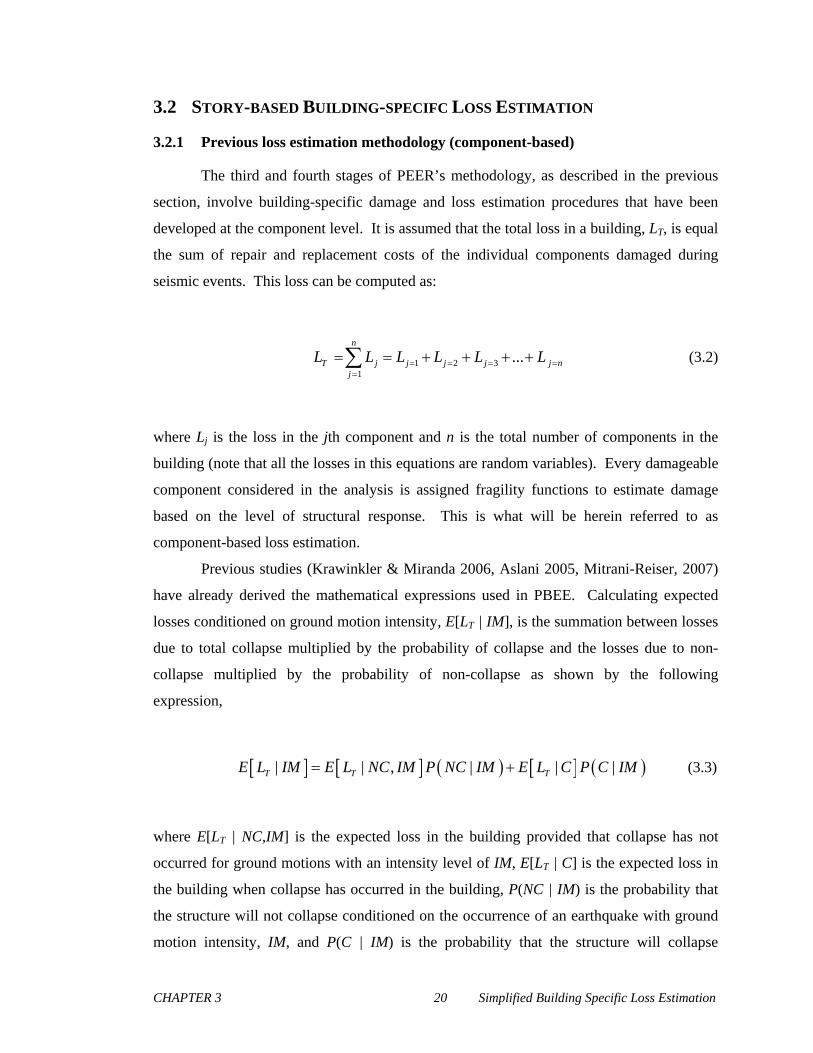
CHAPTER 3 20 Simplified Building Specific Loss Estimation
3.2 STORY-BASED BUILDING-SPECIFC LOSS ESTIMATION
3.2.1 Previous loss estimation methodology (component-based)
The third and fourth stages of PEER’s methodology, as described in the previous
section, involve building-specific damage and loss estimation procedures that have been
developed at the component level. It is assumed that the total loss in a building, LT, is equal
the sum of repair and replacement costs of the individual components damaged during
seismic events. This loss can be computed as:
1 2 31
...n
T j j j j j nj
L L L L L L
(3.2)
where Lj is the loss in the jth component and n is the total number of components in the
building (note that all the losses in this equations are random variables). Every damageable
component considered in the analysis is assigned fragility functions to estimate damage
based on the level of structural response. This is what will be herein referred to as
component-based loss estimation.
Previous studies (Krawinkler & Miranda 2006, Aslani 2005, Mitrani-Reiser, 2007)
have already derived the mathematical expressions used in PBEE. Calculating expected
losses conditioned on ground motion intensity, E[LT | IM], is the summation between losses
due to total collapse multiplied by the probability of collapse and the losses due to non-
collapse multiplied by the probability of non-collapse as shown by the following
expression,
| | , | | |T T TE L IM E L NC IM P NC IM E L C P C IM (3.3)
where E[LT | NC,IM] is the expected loss in the building provided that collapse has not
occurred for ground motions with an intensity level of IM, E[LT | C] is the expected loss in
the building when collapse has occurred in the building, P(NC | IM) is the probability that
the structure will not collapse conditioned on the occurrence of an earthquake with ground
motion intensity, IM, and P(C | IM) is the probability that the structure will collapse
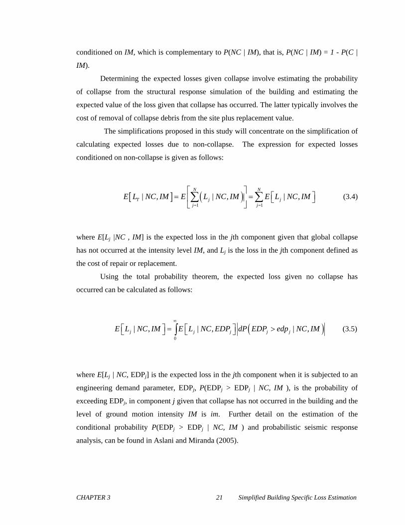
CHAPTER 3 21 Simplified Building Specific Loss Estimation
conditioned on IM, which is complementary to P(NC | IM), that is, P(NC | IM) = 1 - P(C |
IM).
Determining the expected losses given collapse involve estimating the probability
of collapse from the structural response simulation of the building and estimating the
expected value of the loss given that collapse has occurred. The latter typically involves the
cost of removal of collapse debris from the site plus replacement value.
The simplifications proposed in this study will concentrate on the simplification of
calculating expected losses due to non-collapse. The expression for expected losses
conditioned on non-collapse is given as follows:
1 1
| , | , | ,N N
T j jj j
E L NC IM E L NC IM E L NC IM
(3.4)
where E[Lj |NC , IM] is the expected loss in the jth component given that global collapse
has not occurred at the intensity level IM, and Lj is the loss in the jth component defined as
the cost of repair or replacement.
Using the total probability theorem, the expected loss given no collapse has
occurred can be calculated as follows:
0
| , | , | ,j j j j jE L NC IM E L NC EDP dP EDP edp NC IM
(3.5)
where E[Lj | NC, EDPj] is the expected loss in the jth component when it is subjected to an
engineering demand parameter, EDPj, P(EDPj > EDPj | NC, IM ), is the probability of
exceeding EDPj, in component j given that collapse has not occurred in the building and the
level of ground motion intensity IM is im. Further detail on the estimation of the
conditional probability P(EDPj > EDPj | NC, IM ) and probabilistic seismic response
analysis, can be found in Aslani and Miranda (2005).

CHAPTER 3 22 Simplified Building Specific Loss Estimation
The expected loss in component j conditioned on EDP, E[Lj | NC, EDPj] is a
function of the component’s repair cost when it is in different damage states and the
probability of being in each damage state as illustrated in the following expression:
1
[ | , ] | , | ,m
j j j i i ji
E L NC EDP E L NC DS P DS ds NC EDP
(3.6)
where m is the number of damage states in the jth component, E[Lj | NC, DSi] is the
expected value of the normalized loss in component j when it is in damage state i , DSi, and
P(DS = dsi | NC, EDPj) is the probability of the jth component being in damage state i, dsi ,
given that it is subjected to a demand of EDPj. The probability of being in each damage
state for component j can be obtained from component-specific fragility functions. The
reader is referred to Aslani and Miranda (2005) for further details on the development of
component-specific fragility functions.
3.2.2 EDP-DV function formulation
The first step in developing story EDP-DV functions is collapsing out the third
intermediate step of damage estimation by combining information from loss functions and
fragility function as shown in equation (3.6). This requires consolidating all the fragility
and expected repair costs for each component. However, if the repair costs are normalized
by the component’s replacement value, aj, this computation can be conducted without
having to provide these values for every damage state, which will save a substantial amount
of number keeping. Mathematically, aj can be factored out of equation (3.6), and canceled
on both sides equations such that:
1
[ | , ] | , | ,m
j j j j j i i ji
a E L NC EDP a E L NC DS P DS ds NC EDP
(3.7)
where E’[Lj | NC, DSi] and E’[Lj | NC, EDPi] are now normalized by the component’s
replacement value, aj.

CHAPTER 3 23 Simplified Building Specific Loss Estimation
The second step involves summing the individual component losses for the entire
story of a building. Previously, this summation requires inventorying the number of
components and the value of each component type. However, generic EDP-DV functions
can be formulated if components of the same type are grouped together and assumed to
experience the same level of damage (i.e. all partitions in the same story experience the
same level of damage). The loss for each component type can be calculated by multiplying
the results of equation (3.7) by its value relative to entire value of the story, bj (that is, bj is
equal to the total value of components of the same type, j¸ divided by the total value of the
story). Component types can then by summed for the entire story using:
[ | , ] [ | , ]m
STORY k j j jj
E L NC EDP b E L NC EDP (3.8)
where [ | , ]STORY kE L NC EDP is the expected loss of the entire story normalized by the
replacement value of the story, conditioned on the kth EDP. This is how the generic EDP-
DV functions will be expressed. With the loss expressed in these terms, the analysts no
longer needs to specify j replacement values for each component, but rather only needs to
stipulate the total value of the story to determine the loss of the component. The monetary
value of the expected loss for the entire story can then be found with the following
equation:
[ | , ] [ | , ]STORY k l STORY kE L NC EDP c E L NC EDP (3.9)
where [ | , ]STORY kE L NC EDP is the economic loss of the story expressed in dollars and cl is
the replacement value of the story in dollars.
Note that because the results of equations (3.8) and (3.9) are conditioned on EDP,
separate functions need to be generated for each type of EDP sensitivity. EDP sensitivity
is defined by what type of EDP is used to determine building component damage.
Although there are many types of EDPs, the loss estimation process can be further
simplified if the choice of different EDPs is limited to a small number. The EDPs chosen in

CHAPTER 3 24 Simplified Building Specific Loss Estimation
this study are interstory drift ratio (IDR) and peak floor accelerations (PFA). Accordingly,
components can be categorized as either drift-sensitive or acceleration sensitive, depending
which type of parameter induces damage for each component. It is also useful for engineers
to differentiate between structural and nonstructural components. Assuming that structural
damage is primarily caused by IDR, it was determined that only the following seismic
sensitivities would be considered in this implementation: drift-sensitive structural
components, drift-sensitive nonstructural components, and acceleration sensitive
nonstructural components.
An important consideration when formulating EDP-DV functions is whether or not
the economic losses of components on the same story are dependent on one another due to
spatial and physical interactions between the components. This issue is described and
explored in greater detail in section 3.5 of this chapter. For the EDP-DV functions
presented in this study, it was found that these types of losses did not have a large influence
on the total economic losses for each story. However, this may not necessarily always be
the case for other types of structural systems and occupancies and a method of accounting
for these types of losses into EDP-DV functions is presented.
3.3 DATA FOR EDP-DV FUNCTIONS
3.3.1 Building Components & Cost Distributions
Generic story EDP-DV functions normalized by the story replacement value
requires knowing typical cost distributions for a given building occupancy and structural
system. The source chosen to establish the cost distribution for this investigation is the
2007 RS Means Square Foot Costs (Balboni, 2007). The publication gives cost
distributions of the entire building rather than the distributions at the story level.
Engineering judgment was used translate this data into story cost distributions, while
maintaining the overall building cost distribution.
Translating the building cost distribution to story distributions requires making
assumptions as to how the value varies along its height. This will be highly dependent on
how the building components are distributed amongst the different floors, which is typically
a function of the occupancy of the building. The sample functions generated by this study
are for typical commercial office buildings. Although different story cost distributions
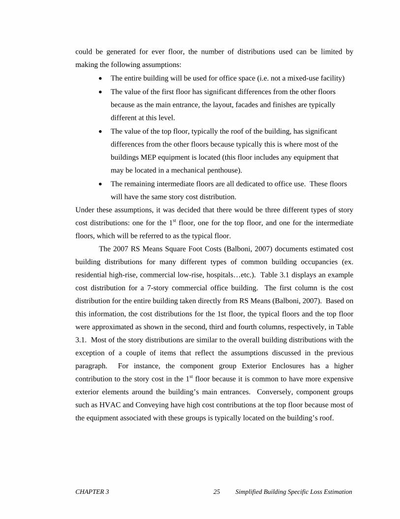
CHAPTER 3 25 Simplified Building Specific Loss Estimation
could be generated for ever floor, the number of distributions used can be limited by
making the following assumptions:
The entire building will be used for office space (i.e. not a mixed-use facility)
The value of the first floor has significant differences from the other floors
because as the main entrance, the layout, facades and finishes are typically
different at this level.
The value of the top floor, typically the roof of the building, has significant
differences from the other floors because typically this is where most of the
buildings MEP equipment is located (this floor includes any equipment that
may be located in a mechanical penthouse).
The remaining intermediate floors are all dedicated to office use. These floors
will have the same story cost distribution.
Under these assumptions, it was decided that there would be three different types of story
cost distributions: one for the 1st floor, one for the top floor, and one for the intermediate
floors, which will be referred to as the typical floor.
The 2007 RS Means Square Foot Costs (Balboni, 2007) documents estimated cost
building distributions for many different types of common building occupancies (ex.
residential high-rise, commercial low-rise, hospitals…etc.). Table 3.1 displays an example
cost distribution for a 7-story commercial office building. The first column is the cost
distribution for the entire building taken directly from RS Means (Balboni, 2007). Based on
this information, the cost distributions for the 1st floor, the typical floors and the top floor
were approximated as shown in the second, third and fourth columns, respectively, in Table
3.1. Most of the story distributions are similar to the overall building distributions with the
exception of a couple of items that reflect the assumptions discussed in the previous
paragraph. For instance, the component group Exterior Enclosures has a higher
contribution to the story cost in the 1st floor because it is common to have more expensive
exterior elements around the building’s main entrances. Conversely, component groups
such as HVAC and Conveying have high cost contributions at the top floor because most of
the equipment associated with these groups is typically located on the building’s roof.

CHAPTER 3 26 Simplified Building Specific Loss Estimation
Table 3.1 Example building and story cost distributions for mid-rise office buildings
Total1 1st Floor Typical Floor Top Floor
A. SUBSTRUCTURE2.3% 0.0% 0.0% 0.0%
B. SHELLB10 Superstructure 17.6% 17.9% 18.5% 15.4%B20 Exterior Enclosure 16.3% 18.8% 16.2% 16.9%B30 Roofing 0.6% 0.0% 0.0% 4.5%
C. INTERIORS19.4% 20.7% 21.4% 11.1%
D. SERVICESD10 Conveying 9.5% 9.1% 9.4% 11.8%D20 Plumbing 1.9% 1.9% 1.9% 2.0%D30 HVAC 13.0% 12.3% 12.7% 17.6%D40 Fire Protection 2.6% 2.6% 2.7% 2.8%D50 Electrical 16.8% 16.6% 17.2% 17.9%
100% 100% 100% 100%Notes: 1) Cost distribution of total bldg value take from RS Means Square Foot Costs (2007)
Building Distribution (% of total bldg value)
Component GroupStory Distribution (% of story value)
Table 3.2 goes into greater detail of the story cost distribution for a typical story in
a 7-story office building by further dividing the cost of each component group into
individual components. The distribution of cost for each component group was primarily
based on engineering judgment. Also included in the table is information about each
component’s seismic sensitivity and assigned fragility group. Several of the components
were assumed to only be damaged if the entire structure collapsed. These components,
termed “rugged,” were assumed to not contribute to the loss due to non-collapse. The
fragilities assigned to the components that are deemed damageable are explained in greater
detail in Section 3.3.2. All the cost distributions for low-rise, mid-rise and high-rise
buildings used in this study can be found in Appendix A.

CHAPTER 3 27 Simplified Building Specific Loss Estimation
Table 3.2 Example component cost distribution for a typical story in a mid-rise office building
Building Height: Mid-riseFloor Type: Typical Floor
Component Seismic Sensitivity Fragility Group
B. SHELLB10 Superstructure
Slab Rugged 8.2%Beam-column Assembly IDR Structural 7.2%Slab-column Assembly IDR Structural 3.1%
B20 Exterior EnclosureExterior Walls IDR Partitions 9.1%Exterior Windows IDR Windows 6.2%Exterior Doors IDR Partitions 1.0%
B30 RoofingRoof Coverings Rugged 0.0%Roof Openings Rugged 0.0%
C. INTERIORSPartitions with finishes IDR Partitions 4.5%Interior Doors IDR Partitions 1.9%Fittings IDR Generic-Drift 0.6%Stair Construction IDR Generic-Drift 1.9%Floor Finishes - 60% carpet IDR DS3 Partition-like 4.4%
30% vinyl composite tile Rugged 2.2%10% ceramic tile Rugged 0.7%
Ceiling Finishes PFA Ceilings 5.1%
D. SERVICESD10 Conveying
Elevators & Lifts IDR Generic-Drift 0.9%PFA Generic-Accl 8.5%
D20 PlumbingPlumbing Fixtures IDR DS3 Partition-like 0.9%
Rugged 1.1%D30 HVAC
Terminal & Package Units PFA Generic-Accl 9.5%IDR Generic-Drift 3.2%
Other HVAC Sys. & Equipment –D40 Fire Protection
Sprinklers PFA Generic-Accl 2.0%Standpipes IDR Generic-Drift 0.7%
D50 ElectricalElectrical Service/Distribution PFA Generic-Accl 1.5%Lighting & Branch Wiring Rugged 1.1%Lighting & Branch Wiring PFA Generic-Accl 5.1%Lighting & Branch Wiring IDR DS3 Partition-like 4.5%Communications & Security Rugged 1.0%Communications & Security PFA Generic-Accl 1.5%Communications & Security IDR DS3 Partition-like 2.5%
= 100% 100%
18.5%
17.2%
Normalized costs
9.4%
16.2%
0.0%
12.7%
2.7%
1.9%
21.4%
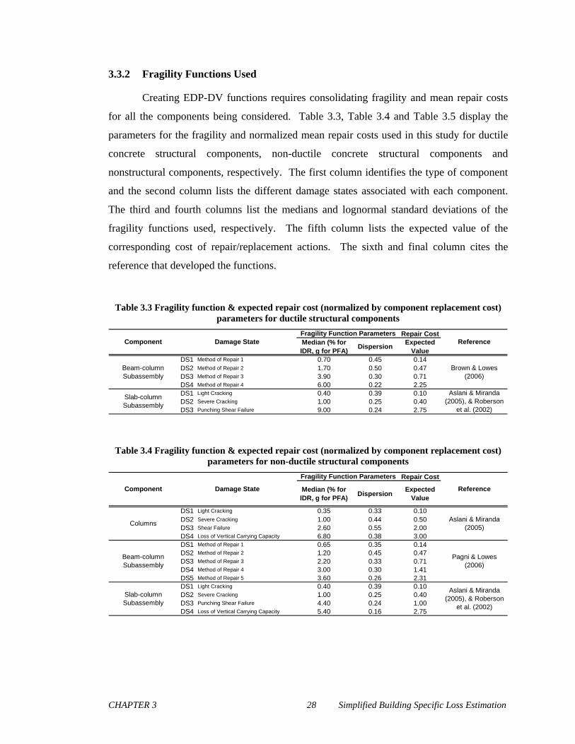
CHAPTER 3 28 Simplified Building Specific Loss Estimation
3.3.2 Fragility Functions Used
Creating EDP-DV functions requires consolidating fragility and mean repair costs
for all the components being considered. Table 3.3, Table 3.4 and Table 3.5 display the
parameters for the fragility and normalized mean repair costs used in this study for ductile
concrete structural components, non-ductile concrete structural components and
nonstructural components, respectively. The first column identifies the type of component
and the second column lists the different damage states associated with each component.
The third and fourth columns list the medians and lognormal standard deviations of the
fragility functions used, respectively. The fifth column lists the expected value of the
corresponding cost of repair/replacement actions. The sixth and final column cites the
reference that developed the functions.
Table 3.3 Fragility function & expected repair cost (normalized by component replacement cost) parameters for ductile structural components
Repair CostMedian (% for IDR, g for PFA)
DispersionExpected
ValueDS1 Method of Repair 1 0.70 0.45 0.14DS2 Method of Repair 2 1.70 0.50 0.47DS3 Method of Repair 3 3.90 0.30 0.71DS4 Method of Repair 4 6.00 0.22 2.25DS1 Light Cracking 0.40 0.39 0.10DS2 Severe Cracking 1.00 0.25 0.40DS3 Punching Shear Failure 9.00 0.24 2.75
Reference
Brown & Lowes (2006)
Aslani & Miranda (2005), & Roberson
et al. (2002)
Slab-column Subassembly
Beam-column Subassembly
Fragility Function ParametersDamage StateComponent
Table 3.4 Fragility function & expected repair cost (normalized by component replacement cost) parameters for non-ductile structural components
Repair Cost
Median (% for IDR, g for PFA)
DispersionExpected
Value
DS1 Light Cracking 0.35 0.33 0.10DS2 Severe Cracking 1.00 0.44 0.50DS3 Shear Failure 2.60 0.55 2.00DS4 Loss of Vertical Carrying Capacity 6.80 0.38 3.00DS1 Method of Repair 1 0.65 0.35 0.14DS2 Method of Repair 2 1.20 0.45 0.47DS3 Method of Repair 3 2.20 0.33 0.71DS4 Method of Repair 4 3.00 0.30 1.41DS5 Method of Repair 5 3.60 0.26 2.31DS1 Light Cracking 0.40 0.39 0.10DS2 Severe Cracking 1.00 0.25 0.40DS3 Punching Shear Failure 4.40 0.24 1.00DS4 Loss of Vertical Carrying Capacity 5.40 0.16 2.75
Slab-column Subassembly
Columns
Fragility Function Parameters
Damage StateComponent
Beam-column Subassembly
Reference
Aslani & Miranda (2005)
Aslani & Miranda (2005), & Roberson
et al. (2002)
Pagni & Lowes (2006)

CHAPTER 3 29 Simplified Building Specific Loss Estimation
Table 3.5 Fragility function & expected repair cost (normalized by component replacement cost) parameters for nonstructural components
Repair CostMedian (% for IDR, g for PFA)
DispersionExpected
Value
DS1Visible damage and small cracks in gypsum board that can be repaired with taping, pasting and painting
0.21 0.61 0.10
DS2
Extensive crack in gypsum board that can be repaired with replacing the gypsum board, taping, pasting and painting
0.69 0.40 0.60
DS3
Damage to panel and also frame that can be repaired with replacing gypsum board and frame, taping, pasting and painting
1.27 0.45 1.20
DS3 Partition-like DS1 IDR 1.27 0.45 1.20 Aslani (2005)
DS1Some minor damages around the frame that can be repaired with realignment of the window
1.60 0.29 0.10
DS2
Occurrence of cracking at glass panel without any fall-out of the glass that can be repaired with replacing of the glass panel
3.20 0.29 0.60
DS3Part of glass panel falls out of the frame. The damage state can be repaired with replacing of glass panel
3.60 0.27 1.20
DS1 Slight Damage 0.55 0.60 0.03DS2 Moderage Damage 1.00 0.50 0.10DS3 Extensive Damage 2.20 0.40 0.60DS4 Complete Damage 3.50 0.35 1.20
DS1
Hanging wires are splayed and few panels fall down. The damage state can be repaired with fixing the hanging wires and replacing the fallen panel.
0.30 0.40 0.12
DS2
Damage to some of main runners and cross tee bars in addition to hanging wires. The damage state can be repaired with replacing the damaged parts of grid, fallen panels and damaged hanging wires.
0.65 0.50 0.36
DS3
Ceiling grid tilts downward (near collapse). The damage state can be repaired with replacing the ceiling and panels.
1.28 0.55 1.20
DS1 Slight Damage 0.70 0.50 0.02DS2 Moderage Damage 1.00 0.50 0.12DS3 Extensive Damage 2.20 0.40 0.36DS4 Complete Damage 3.50 0.35 1.20
ATC (2007)
Partitions (including façade)
Windows
Generic-Drift
IDR
Ramirez & Miranda (2009)
Reference
Ceilings
Generic-Acceleration
ATC (2007)
Aslani & Miranda (2005)
Ramirez & Miranda (2009)
Fragility Function ParametersDamage StateComponent
PFA
Seismic Sensitivity
IDR
IDR
PFA
Most of the fragility functions were used directly from the reference cited in Table
3.5, without any additional modifications. However, several of the structural fragilities
required making assumptions to establish the functions’ parameters. The following section
will detail the assumptions and modifications to the made for this study.
3.3.2.1 Fragility functions for ductile reinforced concrete structural components
Fragility functions for beam-column subassemblies were based on Brown and
Lowes (2006), with slight modifications made to the parameters by the authors of this
study. The lognormal standard deviation of damage state 1 (DS1) was decreased from 0.89
to 0.45 because the original dispersion value published is substantially higher than other
values of dispersion for structural component fragility functions computed from
experimental data. A high value of dispersion in the first damage state of a component can

CHAPTER 3 30 Simplified Building Specific Loss Estimation
be problematic because it can estimate that the probability of damage occurring initiates at
very early levels of IDR. To demonstrate this, damage initiation in a building component
will be quantitatively defined as the value IDR that results in a 1% probability of the first
damage state occurring or being exceeded. Using this criterion, the original parameters of
the function for DS1 published by Brown and Lowes (2006) computes that damage initiates
at an IDR of 0.00085. This estimates that damage will first become probable when relative
floor displacements are equal to about and 1/8th of an inch (assuming a 13-foot story
height). At this level of relative lateral deformation, structural components will more than
likely still behave elastically and not require any repairs to be made.
There exists a range of initial EDP values, from zero to a threshold value (which
can be referred to as a “quiet zone”), where damage will not occur because the response
parameters below this threshold are not large enough to yield the building components. If
this elastic region is not considered when estimating damage using continuous probability
distributions, economic losses (particularly expected annual losses, which are very sensitive
to losses due to non-collapse at small levels of ground motion intensity, Miranda and
Aslani, 2005) may be overestimated. This is because large probabilities will be computed
at small response parameter values for lognormal distribution functions with large values of
dispersion as shown in this example. Thus the standard deviation for the first damage state
of this component was decreased.
The functions for the other damage states generated by Brown and Lowes (2006)
for this component and other functions computed form previous studies on structural
component fragility functions (Robertson et al. 2002, Aslani and Miranda 2005, Pagni and
Lowes 2006) have lognormal standard deviations that typically range from approximately
0.20 to 0.50. Therefore, this fragility was assigned a lognormal standard deviation of 0.45,
which is on the higher end of this range.
Adjustments made to the other damage states include rounding off the parameters of
damage states 2 and 3. The parameters of damage state 4 were adjusted such that it would
not cross the fragility for damage state 3 (this required more substantial adjustments than
the other modifications, however, this fragility is based on a smaller set of data, and may
not be as reliable as the other functions).
At the time of this publication, there were no fragilities available for ductile slab-
column subassemblies. To account for damage of these components, fragilities for non-
ductile slab-column subassemblies (Aslani and Miranda, 2005) were modified to represent

CHAPTER 3 31 Simplified Building Specific Loss Estimation
how these components would perform if they were ductile. The parameters of damage state
3, accounting for punching shear failure of the slab, needed be increased because more
recent codes have introduced shear reinforcing requirements into their provisions (ACI,
2002). An investigation conducted by Roberson et al. (2002) developed a relationship
between gravity load carried by the slab and the interstory drift at which punching shear
occurs for slab-column subassemblies with shear reinforcement. The median IDR for this
damage state was taken from this relationship by assuming a shear demand-capacity ratio of
0.15. The fourth damage state is defined as the loss of vertical carrying capacity which is
not considered for ductile joints because modern building codes require slab reinforcing
bars run continuous through the column joint, preventing this failure mode from occurring.
3.3.2.2 Fragility functions for non-ductile reinforced concrete structural components
Parameters for non-ductile concrete column fragility functions were taken directly
from Aslani and Miranda (2005). The value of IDR that column shear failure occurs, the
third damage state for this component, is dependent on the amount for axial (gravity) load it
is carrying. Consequently, the parameters of the fragility function for the third damage state
are also a function of the level of axial load creating a fragility surface. To determine the
parameters for this fragility, a relatively low level of axial load was assumed
( 50g cP A f , where P is the axial load, Ag is the gross cross-sectional area of the
column, fc is the compressive strength of the concrete and ’’ is the reinforcement ratio), for
low to mid-rise buildings and intermediate level of axial load ( 150g cP A f ) for high-
rise buildings.
Pagni and Lowes’ (2006) developed fragility functions for modern reinforced
concrete beam-column subassemblies. These functions were used in this study with minor
modifications made to some of their parameters. The dispersion of damage state 1 was
decreased from 0.47 to 0.35 to increase the range of IDR where these components behave
elastically and no damage occurs (i.e. increase the “quiet zone” as described in section
3.3.2.1. The other parameters for this function were adjusted to achieve a better fit with the
empirical data reported in the Pagni and Lowes (2006) paper.
Functions for non-ductile concrete slab-column subassemblies were taken directly
from the study conducted by Aslani and Miranda (2005). The level of deformation at which

CHAPTER 3 32 Simplified Building Specific Loss Estimation
punching shear failure occurs in slab-column subassemblies is a function of the level of
gravity load the slab is carrying, typically represented by the shear demand-capacity ratio
that occurs at a distance d/2 from the column face (where d is the average effective depth of
the slab). The median and dispersion of the fragility function for the third damage state of
these components varies as a function of the level of gravity load resulting in a fragility
surface. For the purposes of this study, a low level of gravity load was assumed, where a
shear demand-capacity ratio of 0.15 was used based on the fact that building’s occupancy is
defined as office use and large gravity loads are not expected for this type of use.
3.3.2.3 Fragility functions for drift-sensitive nonstructural components
Fragility functions derived by Aslani and Miranda (2005) for partitions and windows
and partition-like components were used in this study. Aslani and Miranda (2005)
introduced the concept of “partition-like” components – other components whose loss is
dependent on the damage state of the partition. Many of these components, such as
electrical wiring, plumbing…etc., are often contained within the partitions. If a partition is
damaged to an extent that it needs to be replaced, these other components have to be
replaced as well, regardless if they have been damaged independently. Consequently, these
components were assigned the same fragility as the function for the partition replacement,
the partitions’ third damage state, and were termed “DS3 partition-like components.” This
physical and spatial interaction between partitions and the components contained within the
partitions results in their losses being dependent. There are other building components that
exhibit this type of loss dependency and this phenomenon is discussed and investigated in
further detail in section 3.5. No modifications were made to the parameters of functions for
partitions, DS3 partition-like components, and window and were used as documented by
Aslani and Miranda (2005). For all other components, generic fragility functions derived
from empirical data, as described in Chapter 5 of this dissertation, were used to estimate
damage and loss.
3.3.2.4 Fragility functions for acceleration-sensitive nonstructural components
Ceiling fragility functions taken from preliminary data and documents from the ATC-
58 project (ATC, 2007) were used in this study with only one modification made to its first

CHAPTER 3 33 Simplified Building Specific Loss Estimation
damage state. Recent studies (Badillo-Almaraz et al., 2007) have shown that damage may
initiate at larger accelerations than previously thought. The median of the first damage state
was rounded up from 0.27 and 0.30 to take this into account. All other acceleration-
sensitive components were assigned generic fragility functions formulated from empirical
data as described in Chapter 5 of this dissertation.
3.4 EXAMPLE STORY EDP-DV FUNCTIONS
Example EDP-DV functions were created for several variations of reinforced
concrete moment-resisting frame office buildings. Functions for low-rise, mid-rise and
high-rise structures were calculated. Other structural variations were also considered, such
as frame type (perimeter or space frames) and the ductility of the concrete (ductile or non-
ductile), when generating EDP-DV functions for structural components. For all variations,
functions for the different floor types (1st floor, typical floor and top floor) were formulated.
The entire set of functions computed in this study are reported in Appendix B of this
document.
Figure 3.2 shows the EDP-DV story functions generated for mid-rise, ductile
perimeter frame buildings. Functions for drift-sensitive structural components, drift-
sensitive nonstructural components, and acceleration sensitive nonstructural components
are plotted in Figures (a), (b) and (c) respectively. On each graph, the functions for the 1st
floor, the typical floor and the top floor are plotted.

CHAPTER 3 34 Simplified Building Specific Loss Estimation
Structural components
0.00
0.20
0.40
0.60
0.80
1.00
0.00 0.05 0.10 0.15IDR
E(L | IDR)
1st Floor
Typ Floor
Top Floor
(a)
Structural components
0.00
0.20
0.40
0.60
0.80
1.00
0.00 0.05 0.10 0.15IDR
E(L | IDR)
1st Floor
Typ Floor
Top Floor
(a)
Nonstructural components
0.00
0.20
0.40
0.60
0.80
1.00
0.00 0.05 0.10 0.15IDR
E(L | IDR) Nonstructural components
0.00
0.20
0.40
0.60
0.80
1.00
0.00 2.00 4.00 6.00 8.00PFA [g]
E(L | PFA)
(b) (c)
Nonstructural components
0.00
0.20
0.40
0.60
0.80
1.00
0.00 0.05 0.10 0.15IDR
E(L | IDR) Nonstructural components
0.00
0.20
0.40
0.60
0.80
1.00
0.00 2.00 4.00 6.00 8.00PFA [g]
E(L | PFA)Nonstructural components
0.00
0.20
0.40
0.60
0.80
1.00
0.00 0.05 0.10 0.15IDR
E(L | IDR) Nonstructural components
0.00
0.20
0.40
0.60
0.80
1.00
0.00 2.00 4.00 6.00 8.00PFA [g]
E(L | PFA)
(b) (c)
Figure 3.2 Story EDP-DV functions for typical floors in mid-rise office buildings with ductile reinforced concrete moment resisting perimeter frames.
Comparing plots in Figure 3.2(a) between the different floor types shows that losses
for drift-sensitive structural components are slightly higher for the 1st and typical floors than
the top floor. A similar trend is observed in Figure 3.2(b) for drift sensitive nonstructural
components. Conversely, acceleration-sensitive nonstructural components show the
opposite trend (Figure 3.2(c)), where the larger losses are observed in the top floor. These
trends can be explained by how the cost is distributed along the height of the building.
Drift-sensitive items, such as partitions and structural members, make more of the relative
story value in the lower stories, especially in the 1st floor where more expensive
components (ex. finishes) may be located. On the other hand, acceleration-sensitive
components may make up more of the story value at the top floor because mechanical items
(such as HVAC units) are typically located on the roof of these types of buildings.
CHAPTER 3 35 Simplified Building Specific Loss Estimation
The nonstructural, drift-sensitive functions indicate that these types of components
have the largest potential to contribute to the loss, especially for structural systems that are
designed to experience large IDRs, such as moment-frames. The functions saturate
between 0.46-0.53 of the total value of the story. Further, these functions estimate higher
economic losses at smaller IDR values than the losses estimated by the functions for
structural components. Beginning at an approximate interstory drift of 0.05, these
functions take a steep increase to a loss of about 0.32 of the story value as the IDR
approaches 0.02. By comparison, the structural components experience loss of 0.05 of the
total story value at an IDR of 0.025 (an IDR of 0.025 is a noteworthy value because modern
reinforced concrete moment frame buildings are designed to not to exceed this level of IDR
using equivalent static analyses when subjected to a ground motion intensity equal to the
design-basis earthquake as prescribed by US building codes, ICC 2006), which is about
600% smaller than the drift-sensitive nonstructural components. Previous studies (Aslani
and Miranda 2005, Taghavi and Miranda, 2006) have also suggested that nonstructural
components will make up the majority of seismic-induced losses as observed here. It
follows that if the value of the story is primarily comprised of nonstructural components,
the majority of associated losses will be made up of these elements.
The difference in EDP-DV functions for typical floors between low-rise, mid-rise
and high-rise buildings are shown in Figure 3.3 for each of the three different components
group categories. These figures show that the losses for structural components are lower
for stories in low-rise buildings than the losses in stories of high-rise buildings. The
opposite trend is true for nonstructural components, where the low-rise buildings exhibit the
largest normalized story losses. When Figure 3.3(b) is compared to Figure 3.3(c), it can be
observed that the differences in economic losses between the low-rise and high-rise
buildings are larger for drift-sensitive components than they are for acceleration-sensitive
components. These trends can also be attributed to the differences in cost distributions for
these types of elements between structures of different heights. For instance, the value of
structural components relative to the entire value building increases for taller buildings as
can be observed from the cost distributions in Appendix A (taken from Balboni, 2007).

CHAPTER 3 36 Simplified Building Specific Loss Estimation
Structural components
0.00
0.20
0.40
0.60
0.80
1.00
0.00 0.05 0.10 0.15IDR
E(L | IDR)
Low-rise
Mid-rise
High-rise
(a)
Structural components
0.00
0.20
0.40
0.60
0.80
1.00
0.00 0.05 0.10 0.15IDR
E(L | IDR)
Low-rise
Mid-rise
High-rise
(a)
Nonstructural components
0.00
0.20
0.40
0.60
0.80
1.00
0.00 0.05 0.10 0.15IDR
E(L | IDR) Nonstructural components
0.00
0.20
0.40
0.60
0.80
1.00
0.00 2.00 4.00 6.00 8.00PFA [g]
E(L | PFA)
(b) (c)
Nonstructural components
0.00
0.20
0.40
0.60
0.80
1.00
0.00 0.05 0.10 0.15IDR
E(L | IDR) Nonstructural components
0.00
0.20
0.40
0.60
0.80
1.00
0.00 2.00 4.00 6.00 8.00PFA [g]
E(L | PFA)
(b) (c)
Figure 3.3 EDP-DV Functions for low-rise, mid-rise and high rise ductile reinforced concrete moment frame office buildings
EDP-DV functions can be used to evaluate how varying different structural
parameters can influence loss at the story-level. Over the past 40 years, US seismic
building codes have introduced a variety of provisions to increase the ductility of structural
reinforced concrete. Based on observed performance during seismic events, more stringent
confinement requirements and other detailing provisions that delay or prevent certain
sudden, failure modes from occurring (ex. shear failure modes), were instituted to decrease
the probability of lives lost during an earthquake. How this improved performance
translates when using losses as a metric can be assessed using the EDP-DV functions
formulated in this study. Figure 3.4 compares structural story functions between ductile
and non-ductile concrete elements. Both functions initiate loss at approximately the same
IDR, but begin to deviate from each other at an IDR of about 0.015. The non-ductile
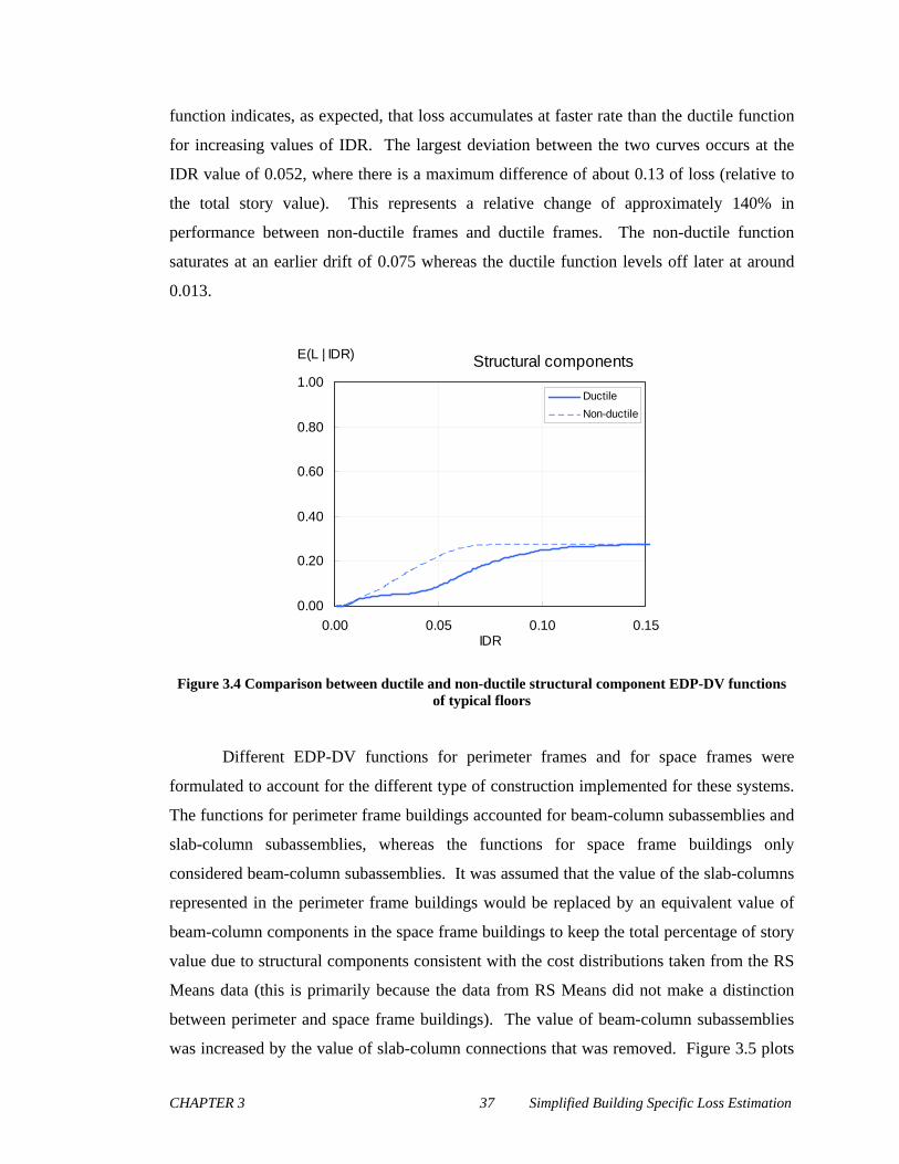
CHAPTER 3 37 Simplified Building Specific Loss Estimation
function indicates, as expected, that loss accumulates at faster rate than the ductile function
for increasing values of IDR. The largest deviation between the two curves occurs at the
IDR value of 0.052, where there is a maximum difference of about 0.13 of loss (relative to
the total story value). This represents a relative change of approximately 140% in
performance between non-ductile frames and ductile frames. The non-ductile function
saturates at an earlier drift of 0.075 whereas the ductile function levels off later at around
0.013.
Structural components
0.00
0.20
0.40
0.60
0.80
1.00
0.00 0.05 0.10 0.15IDR
E(L | IDR)
Ductile
Non-ductile
Figure 3.4 Comparison between ductile and non-ductile structural component EDP-DV functions of typical floors
Different EDP-DV functions for perimeter frames and for space frames were
formulated to account for the different type of construction implemented for these systems.
The functions for perimeter frame buildings accounted for beam-column subassemblies and
slab-column subassemblies, whereas the functions for space frame buildings only
considered beam-column subassemblies. It was assumed that the value of the slab-columns
represented in the perimeter frame buildings would be replaced by an equivalent value of
beam-column components in the space frame buildings to keep the total percentage of story
value due to structural components consistent with the cost distributions taken from the RS
Means data (this is primarily because the data from RS Means did not make a distinction
between perimeter and space frame buildings). The value of beam-column subassemblies
was increased by the value of slab-column connections that was removed. Figure 3.5 plots

CHAPTER 3 38 Simplified Building Specific Loss Estimation
the comparison between different frame types for typical floors of mid-rise buildings. The
graph shows that there is very little difference in story loss between the two types of frames.
The maximum difference in loss – approximately 0.035 of the total story value – occurs
between the IDR range of 0.06 to 0.08. The relatively small difference in the functions may
suggest that it may not be important to differentiate between frame type when evaluating
non-collapse losses. Being able to make this assumption can further simplify the process in
assessing loss by not having to define and use separate EDP-DV functions for perimeter and
space frames separately.
Structural components
0.00
0.20
0.40
0.60
0.80
1.00
0.00 0.05 0.10 0.15IDR
E(L | IDR)
Perimeter
Space
Figure 3.5 Comparison of structural EDP-DV functions between perimeter and space frame type structures
As documented in section 3.3.2, several components have fragility functions whose
parameters are dependent on other variables. For instance, the probability of experiencing
or exceeding the damage state for shear punching failure of slab-column connections is
dependent on the amount of gravity load the slab is carrying (Aslani and Miranda, 2005).
Assumptions on the level of demand-capacity shear load ratio needed to be made to set the
median and dispersion to be used in calculating the EDP-DV function. This assumption
was evaluated by generating functions for both low and high levels of gravity loads to see
how sensitive this parameter affects the corresponding losses, and the results are shown in
Figure 3.6.

CHAPTER 3 39 Simplified Building Specific Loss Estimation
The primary differences between these two EDP-DV functions are the parameters
used for the fragility function of the third damage state of the slab-column connections
(punching shear failure). For the fragility assuming a low level of gravity load (shear
demand-capacity ratio = 0.15), the median IDR was computed to be 0.09 (based on
Robertson et al, 2002) with a lognormal standard deviation of 0.24 (based on Aslani and
Miranda, 2005). For the fragility assuming a high-level of gravity load (shear demand-
capacity ratio = 0.50), the median was IDR was computed to be 0.056 (based on Robertson
et al, 2002) with a lognormal standard deviation of 0.54 (based on Aslani and Miranda,
2005).
There appears to be some difference between the two functions, however, it does
not seem to be very substantial. Largest difference in losses occurs within the IDR range of
0.05 and 0.10, where the maximum difference in loss (0.05 of the story value) occurs at
around and IDR of 0.075. This represents a relative difference of 28% if the gravity load is
underestimated using the lower level assumption. This suggests that the assumed gravity
load on these components for perimeter frames may not have as strong an influence on
seismic-induced losses as other structural properties (i.e. ductility of concrete). Analysts
conducting loss assessments can take advantage of the fact that this assumption will not
affect their estimates significantly, by not having to deal with multiple functions that
account for different levels of gravity load.
Structural components
0.00
0.20
0.40
0.60
0.80
1.00
0.00 0.05 0.10 0.15IDR
E(L | IDR)
Low gravity load
High gravity load
Figure 3.6 Influence of varying assumed gravity load on slab-column subassemblies on structural EDP-DV functions
CHAPTER 3 40 Simplified Building Specific Loss Estimation
3.5 CONDITIONAL LOSS OF SPATIALLY INTERDEPENDENT COMPONENTS
Consolidating the loss components into story EDP-DV functions in this manner
provides the opportunity to investigate the issue of the interaction between the losses of
components that are spatially interdependent. These types of losses occurs when damage
from one component results in repair or replacement of another component because of their
physical relationship between the two elements. For instance, when sprinklers are
damaged, water may leak onto the components below, such as suspended lighting fixtures.
The fragility functions of lighting fixtures typically do not capture damage due to leaking
water, but still needs to be considered if losses are to be computed accurately.
The spatial interaction of components will influence economic loss estimates when
the fragility functions of the elements begin to significantly overlap. To illustrate this,
Figure 3.7 shows two example sets of hypothetical fragility functions for sprinklers and
suspending lighting fixtures, which may interact during a seismic event. Each figure, (a)
and (b), plots functions for two damage states, one in which repair is required (DM1) and
the other in which replacement is required (DM2), for both the suspended lighting (solid
lines) and the sprinklers (dashed lines). In this example, when the sprinklers’ first damage
state occurs, water leakage is assumed to occur as well damaging the lighting fixtures below
and initiating replacement of the lighting fixtures. If the components have fragilities as
those shown in Figure 3.7 (a), then this spatially interaction does not have that large of
influence on the economic losses. For instance, for a given PFA = 1.0g, the probability of
the light fixtures requiring replacement is 9%, whereas the probability of the sprinklers
leaking and needing repair is approximately 0%. This means that it is more likely that if the
lighting fixtures need replacement due to the accelerations induced by the applied ground
motion, rather than due to water leakage of damaged sprinklers. In this case the losses are
calculated correctly because for the given level of PFA there is almost no probability that
losses of lighting fixture replacement due to water damage will be incurred.
Conversely, if the components have fragilities that have greater overlap as shown in
Figure 3.7 (b), damage and loss estimation may be underestimated. In this case, at a PFA =
1.0 the probability of the sprinklers leaking and forcing replacement of the lighting fixtures
(24%) is higher than the probability of lighting fixture being replaced due to floor

CHAPTER 3 41 Simplified Building Specific Loss Estimation
accelerations directly (9%). There is a significant probability that the lighting fixture will
have to be replaced due to water damage, however, the only monetary losses that are
associated with this damage state (Sprinklers -DM1) are the repair costs of the sprinklers.
When economic losses are computed for the lighting fixtures, the methodology discussed
thus far will only account for losses due to damage caused by PFA directly and not water
damage. This approach ignores the interaction between the components (i.e. the
components’ losses are treated independent of one another). There is nothing in the current
framework that accounts for the conditional loss of replacing the lighting due to water
damage.
Previous studies (Beck et al., 2002), have attempted to account for these types of
conditional economic losses due to spatial interaction by including the replacement cost of
the dependent component into the other component’s repair cost. In the previous example
for a given PFA = 1.0g , this approach includes the cost of replacing the suspended lighting
fixtures into the repair cost associated with the first damage state of the sprinklers (DM1 –
Repair). Unfortunately, monetary losses from the replacement of the lighting fixtures due
to PFA directly are still computed because this event has a probability (9%) of occurring for
the given level of EDP. Consequently, the economic loss from the cost of replacing the
lighting fixtures is counted twice, or “double counted.”
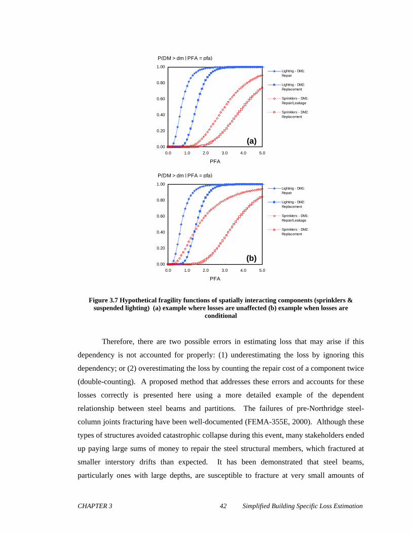
CHAPTER 3 42 Simplified Building Specific Loss Estimation
0.00
0.20
0.40
0.60
0.80
1.00
0.0 1.0 2.0 3.0 4.0 5.0
PFA
Lighting - DM1:Repair
Lighting - DM2:Replacement
Sprinklers - DM1:Repair/Leakage
Sprinklers - DM2:Replacement
P(DM > dm | PFA = pfa)
0.00
0.20
0.40
0.60
0.80
1.00
0.0 1.0 2.0 3.0 4.0 5.0
PFA
Lighting - DM1:Repair
Lighting - DM2:Replacement
Sprinklers - DM1:Repair/Leakage
Sprinklers - DM2:Replacement
P(DM > dm | PFA = pfa)
(a)
(b)
0.00
0.20
0.40
0.60
0.80
1.00
0.0 1.0 2.0 3.0 4.0 5.0
PFA
Lighting - DM1:Repair
Lighting - DM2:Replacement
Sprinklers - DM1:Repair/Leakage
Sprinklers - DM2:Replacement
P(DM > dm | PFA = pfa)
0.00
0.20
0.40
0.60
0.80
1.00
0.0 1.0 2.0 3.0 4.0 5.0
PFA
Lighting - DM1:Repair
Lighting - DM2:Replacement
Sprinklers - DM1:Repair/Leakage
Sprinklers - DM2:Replacement
P(DM > dm | PFA = pfa)
(a)
(b)
Figure 3.7 Hypothetical fragility functions of spatially interacting components (sprinklers & suspended lighting) (a) example where losses are unaffected (b) example when losses are
conditional
Therefore, there are two possible errors in estimating loss that may arise if this
dependency is not accounted for properly: (1) underestimating the loss by ignoring this
dependency; or (2) overestimating the loss by counting the repair cost of a component twice
(double-counting). A proposed method that addresses these errors and accounts for these
losses correctly is presented here using a more detailed example of the dependent
relationship between steel beams and partitions. The failures of pre-Northridge steel-
column joints fracturing have been well-documented (FEMA-355E, 2000). Although these
types of structures avoided catastrophic collapse during this event, many stakeholders ended
up paying large sums of money to repair the steel structural members, which fractured at
smaller interstory drifts than expected. It has been demonstrated that steel beams,
particularly ones with large depths, are susceptible to fracture at very small amounts of
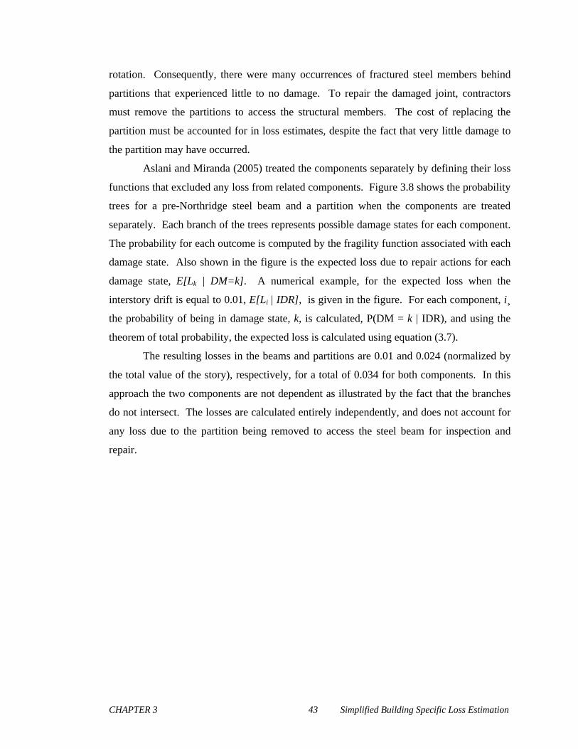
CHAPTER 3 43 Simplified Building Specific Loss Estimation
rotation. Consequently, there were many occurrences of fractured steel members behind
partitions that experienced little to no damage. To repair the damaged joint, contractors
must remove the partitions to access the structural members. The cost of replacing the
partition must be accounted for in loss estimates, despite the fact that very little damage to
the partition may have occurred.
Aslani and Miranda (2005) treated the components separately by defining their loss
functions that excluded any loss from related components. Figure 3.8 shows the probability
trees for a pre-Northridge steel beam and a partition when the components are treated
separately. Each branch of the trees represents possible damage states for each component.
The probability for each outcome is computed by the fragility function associated with each
damage state. Also shown in the figure is the expected loss due to repair actions for each
damage state, E[Lk | DM=k]. A numerical example, for the expected loss when the
interstory drift is equal to 0.01, E[Li | IDR], is given in the figure. For each component, i¸
the probability of being in damage state, k, is calculated, P(DM = k | IDR), and using the
theorem of total probability, the expected loss is calculated using equation (3.7).
The resulting losses in the beams and partitions are 0.01 and 0.024 (normalized by
the total value of the story), respectively, for a total of 0.034 for both components. In this
approach the two components are not dependent as illustrated by the fact that the branches
do not intersect. The losses are calculated entirely independently, and does not account for
any loss due to the partition being removed to access the steel beam for inspection and
repair.
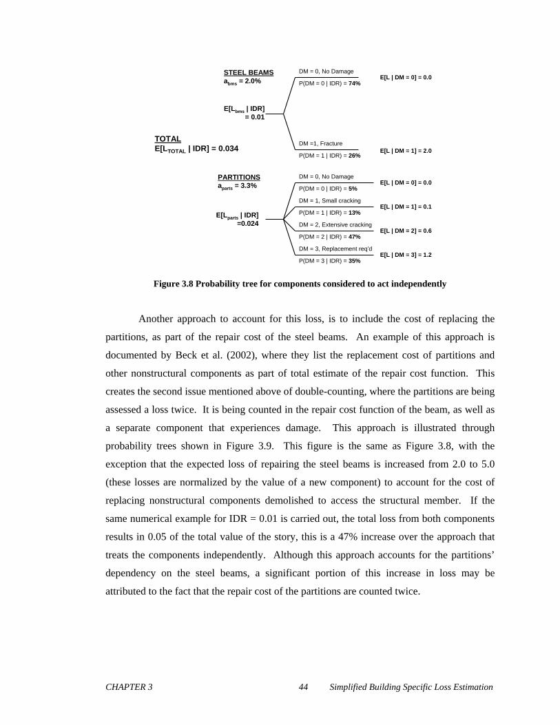
CHAPTER 3 44 Simplified Building Specific Loss Estimation
DM = 0, No Damage
DM =1, Fracture
E[Lbms | IDR] = 0.01
P(DM = 0 | IDR) = 74%
P(DM = 1 | IDR) = 26%
E[L | DM = 0] = 0.0
E[L | DM = 1] = 2.0
DM = 0, No Damage
DM = 3, Replacement req’d
E[Lparts | IDR]=0.024
DM = 1, Small cracking
DM = 2, Extensive cracking
P(DM = 0 | IDR) = 5%
P(DM = 1 | IDR) = 13%
P(DM = 2 | IDR) = 47%
P(DM = 3 | IDR) = 35%
E[L | DM = 0] = 0.0
E[L | DM = 1] = 0.1
E[L | DM = 2] = 0.6
E[L | DM = 3] = 1.2
STEEL BEAMSabms = 2.0%
PARTITIONSaparts = 3.3%
TOTALE[LTOTAL | IDR] = 0.034
Figure 3.8 Probability tree for components considered to act independently
Another approach to account for this loss, is to include the cost of replacing the
partitions, as part of the repair cost of the steel beams. An example of this approach is
documented by Beck et al. (2002), where they list the replacement cost of partitions and
other nonstructural components as part of total estimate of the repair cost function. This
creates the second issue mentioned above of double-counting, where the partitions are being
assessed a loss twice. It is being counted in the repair cost function of the beam, as well as
a separate component that experiences damage. This approach is illustrated through
probability trees shown in Figure 3.9. This figure is the same as Figure 3.8, with the
exception that the expected loss of repairing the steel beams is increased from 2.0 to 5.0
(these losses are normalized by the value of a new component) to account for the cost of
replacing nonstructural components demolished to access the structural member. If the
same numerical example for IDR = 0.01 is carried out, the total loss from both components
results in 0.05 of the total value of the story, this is a 47% increase over the approach that
treats the components independently. Although this approach accounts for the partitions’
dependency on the steel beams, a significant portion of this increase in loss may be
attributed to the fact that the repair cost of the partitions are counted twice.

CHAPTER 3 45 Simplified Building Specific Loss Estimation
DM = 0, No Damage
DM =1, Fracture
E[Lbms | IDR] = 0.026
P(DM = 0 | IDR) = 74%
P(DM = 1 | IDR) = 26%
E[L | DM = 0] = 0.0
E[L | DM = 1] = 5.0
DM = 0, No Damage
DM = 3, Replacement req’d
E[Lparts | IDR]=0.024
DM = 1, Small cracking
DM = 2, Extensive cracking
P(DM = 0 | IDR) = 5%
P(DM = 1 | IDR) = 13%
P(DM = 2 | IDR) = 47%
P(DM = 3 | IDR) = 35%
E[L | DM = 0] = 0.0
E[L | DM = 1] = 0.1
E[L | DM = 2] = 0.6
E[L | DM = 3] = 1.2
STEEL BEAMSabms = 2.0%
PARTITIONSaparts = 3.3%
TOTALE[LTOTAL | IDR] = 0.05
DM = 0, No Damage
DM =1, Fracture
E[Lbms | IDR] = 0.026
P(DM = 0 | IDR) = 74%
P(DM = 1 | IDR) = 26%
E[L | DM = 0] = 0.0
E[L | DM = 1] = 5.0
DM = 0, No Damage
DM = 3, Replacement req’d
E[Lparts | IDR]=0.024
DM = 1, Small cracking
DM = 2, Extensive cracking
P(DM = 0 | IDR) = 5%
P(DM = 1 | IDR) = 13%
P(DM = 2 | IDR) = 47%
P(DM = 3 | IDR) = 35%
E[L | DM = 0] = 0.0
E[L | DM = 1] = 0.1
E[L | DM = 2] = 0.6
E[L | DM = 3] = 1.2
STEEL BEAMSabms = 2.0%
PARTITIONSaparts = 3.3%
TOTALE[LTOTAL | IDR] = 0.05
Figure 3.9 Probability tree for independent components that use double-counting to account for dependency
Thus far we have demonstrated that the first approach ignores the loss produced by
repair actions that affect more than one component, therefore, may be underestimating the
combined loss of both components. Although the second method accounts for this
dependency, it may be overestimating the loss because it double counts the repair of the
dependent component. The actual loss will be somewhere in between the two methods.
Therefore an approach that captures this dependency without double-counting is required.
The proposed approach computes the loss such that the estimation of the dependent
components’ damage is conditional on the damage state of the other component. Figure
3.10 shows the probability tree that illustrates this method. The partitions’ damage is now
conditional on what damage state the steel beams are in, as represented by the branches of
the partitions being stacked behind those of the beams. If the steel beam does not
experience damage, the partitions’ damage is estimated by using the same fragility
functions as before. If the beam has been damaged, then only two possible damage states
are considered: no damage and replacement required. Note that the replacement damage
state is assigned a conditional probability of 100% to ensure that the partition will be
replaced if we know that the beam has fractured.
CHAPTER 3 46 Simplified Building Specific Loss Estimation
DM = 0, No Damage
DM =1, Fracture
E[LTOTAL | IDR] = 0.038
P(DM = 0 | IDR) = 74%
P(DM = 1 | IDR) = 26%
DM = 0, No Damage
DM = 3, Replacement req’d
DM = 1, Small cracking
DM = 2, Extensive cracking
P(DM = 0 | IDR) = 5%
P(DM = 1 | IDR) = 13%
P(DM = 2 | IDR) = 47%
P(DM = 3 | IDR) = 35%
DM = 0, No Damage
DM = 3, Replacement req’d
P(DM = 0 | IDR) = 0%
P(DM = 3 | IDR) = 100%
E[L | DM = 0] = 0.0
E[L | DM = 1] = 0.1
E[L | DM = 2] = 0.6
E[L | DM = 3] = 1.2
E[L | DM = 0] = 0.0
E[L | DM = 1] = 2.0
STEEL BEAMSabms = 2.0%
PARTITIONSaparts = 3.3%
TOTAL
DM = 0, No Damage
DM =1, Fracture
E[LTOTAL | IDR] = 0.038
P(DM = 0 | IDR) = 74%
P(DM = 1 | IDR) = 26%
DM = 0, No Damage
DM = 3, Replacement req’d
DM = 1, Small cracking
DM = 2, Extensive cracking
P(DM = 0 | IDR) = 5%
P(DM = 1 | IDR) = 13%
P(DM = 2 | IDR) = 47%
P(DM = 3 | IDR) = 35%
DM = 0, No Damage
DM = 3, Replacement req’d
P(DM = 0 | IDR) = 0%
P(DM = 3 | IDR) = 100%
E[L | DM = 0] = 0.0
E[L | DM = 1] = 0.1
E[L | DM = 2] = 0.6
E[L | DM = 3] = 1.2
E[L | DM = 0] = 0.0
E[L | DM = 1] = 2.0
STEEL BEAMSabms = 2.0%
PARTITIONSaparts = 3.3%
TOTAL
Figure 3.10 Probability tree for proposed approach to account for dependent components.
Using the previous numerical example in the descriptions of the previous
approaches, the total probability theorem can be carried though both branches to calculate
that the expected loss from both components is 0.038 given an IDR of 0.01. As expected,
this value is between the values generated by the previous approaches. It 12% greater than
the first approach, where the components’ losses are calculated independently; however, it
is 32% less than if the partition losses are double counted. This infers that double-counting
creates a greater deviation in loss than assuming the components act independently.
Instead at looking at a single value of IDR, a better comparison of the three
approaches can be made by contrasting the resulting EDP-DV functions when both
components are integrated using equation (3.7) over a range of IDRs. Figure 3.11 shows
the EDP-DV functions of all three approaches. It appears that the trends from the numerical
example of the loss at a given IDR = 0.01 can also be observed when comparing EDP-DV
functions. The proposed approach is slightly larger than the approach that treats each
component independently. The approach that double counts loss due to partition repairs,
however, is significantly higher than the proposed approach. Again, this suggests that
double-counting may introduce more error into loss estimates than treating each component
independently

CHAPTER 3 47 Simplified Building Specific Loss Estimation
0.0%
5.0%
10.0%
15.0%
20.0%
25.0%
0.000 0.004 0.008 0.012 0.016 0.020
IDR
E[L | IDR]
Independent
Dependent, w/ Double-counting
Dependent w/o Double-counting
Figure 3.11 EDP-DV functions for three different approaches of handling component dependency
For this particular example, using conditional fragility functions did not have a
significant difference in loss than if the components were treated independently. This can
be explained examining the fragility functions of both components as shown in Figure 3.12.
How much loss increases due to component dependence, depends on how much the fragility
of the steel beam overlaps with the first two damage states of the partitions. If the steel
beams’ fragility overlaps with these damage states, it means that there is a probability that
the beams may fracture, initiating replacement, before small or extensive cracking is
experienced in the partitions. The greater the overlap, the higher this probability is and the
greater expected loss is. Although, these particular components have small levels of
overlap, other dependent components may have greater overlap, and have a more significant
difference in expected losses than if the components were considered independent.
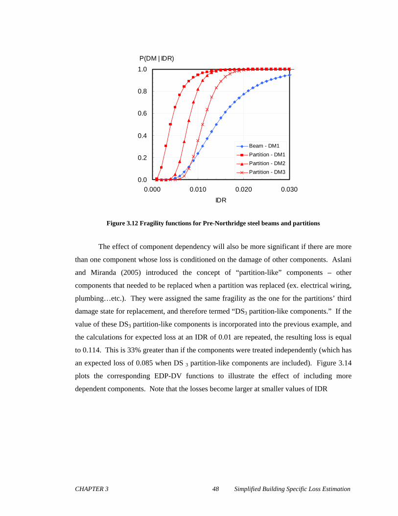
CHAPTER 3 48 Simplified Building Specific Loss Estimation
0.0
0.2
0.4
0.6
0.8
1.0
0.000 0.010 0.020 0.030
IDR
Beam - DM1
Partition - DM1
Partition - DM2
Partition - DM3
P(DM | IDR)
Figure 3.12 Fragility functions for Pre-Northridge steel beams and partitions
The effect of component dependency will also be more significant if there are more
than one component whose loss is conditioned on the damage of other components. Aslani
and Miranda (2005) introduced the concept of “partition-like” components – other
components that needed to be replaced when a partition was replaced (ex. electrical wiring,
plumbing…etc.). They were assigned the same fragility as the one for the partitions’ third
damage state for replacement, and therefore termed “DS3 partition-like components.” If the
value of these DS3 partition-like components is incorporated into the previous example, and
the calculations for expected loss at an IDR of 0.01 are repeated, the resulting loss is equal
to 0.114. This is 33% greater than if the components were treated independently (which has
an expected loss of 0.085 when DS 3 partition-like components are included). Figure 3.14
plots the corresponding EDP-DV functions to illustrate the effect of including more
dependent components. Note that the losses become larger at smaller values of IDR

CHAPTER 3 49 Simplified Building Specific Loss Estimation
DM = 0, No Damage
DM =1, Fracture
E[LTOTAL | IDR] = 0.114
P(DM = 0 | IDR) = 74%
P(DM = 1 | IDR) = 26%
DM = 0, No Damage
DM = 3, Replacement req’d
DM = 1, Small cracking
DM = 2, Extensive cracking
P(DM = 0 | IDR) = 5%
P(DM = 1 | IDR) = 13%
P(DM = 2 | IDR) = 47%
P(DM = 3 | IDR) = 35%
DM = 0, No Damage
DM = 3, Replacement req’d
P(DM = 0 | IDR) = 0%
P(DM = 3 | IDR) = 100%
E[L | DM = 0] = 0.0
E[L | DM = 1] = 0.1
E[L | DM = 2] = 0.6
E[L | DM = 3] = 1.2
E[L | DM = 0] = 0.0
E[L | DM = 1] = 2.0
STEEL BEAMSabms = 2.0%
PARTITIONS & DS3 COMPSaparts = 3.3% & aDS3 = 12.2%
TOTAL
DM = 0, No Damage
DM =1, Fracture
E[LTOTAL | IDR] = 0.114
P(DM = 0 | IDR) = 74%
P(DM = 1 | IDR) = 26%
DM = 0, No Damage
DM = 3, Replacement req’d
DM = 1, Small cracking
DM = 2, Extensive cracking
P(DM = 0 | IDR) = 5%
P(DM = 1 | IDR) = 13%
P(DM = 2 | IDR) = 47%
P(DM = 3 | IDR) = 35%
DM = 0, No Damage
DM = 3, Replacement req’d
P(DM = 0 | IDR) = 0%
P(DM = 3 | IDR) = 100%
E[L | DM = 0] = 0.0
E[L | DM = 1] = 0.1
E[L | DM = 2] = 0.6
E[L | DM = 3] = 1.2
E[L | DM = 0] = 0.0
E[L | DM = 1] = 2.0
STEEL BEAMSabms = 2.0%
PARTITIONS & DS3 COMPSaparts = 3.3% & aDS3 = 12.2%
TOTAL
Figure 3.13 Probability tree for proposed approach, including other DS3 Partition-like components
0.0%
5.0%
10.0%
15.0%
20.0%
25.0%
0.000 0.004 0.008 0.012 0.016 0.020
IDR []
E[L | IDR]
IndependentDependent, w/o Double-counting
Figure 3.14 EDP-DV functions for proposed approach vs treating components independently, with DS3 Partition-like components included.

CHAPTER 3 50 Simplified Building Specific Loss Estimation
3.6 DISCUSSION OF LIMITATIONS OF STORY-BASED APPROACH & EDP-DV FUNCTIONS
The simplifications presented here offer numerous advantages in terms of
computational efficiency and ease of use. Using a story-based approach in combination
with EDP-DV functions to evaluate seismic-induced economic loss is not as complicated or
computationally intensive as component-based methods, while still being able to capture
building-specific behavior – notably higher mode effects of multi-degree of freedom
systems, nonlinear behavior of structures and repair cost variability – that regional loss
estimation methods can not. However, making the simplifications discussed in this chapter
results in limitations on the level of detail of the loss analysis.
The EDP-DV functions formulated in this study compute economic loss two
dimensionally. This means that it is assumed that all components in a story are subjected to
response parameters that act in only one direction and all components experience damage in
same direction (i.e. the approach does not consider structural response that may result from
both directional components of a ground motion nor does it account for the fact that
components may be oriented in different directions). For example, the damage computed
for all partitions in a story is only dependent on one value of IDR even though there may be
structural displacements occurring in both primary planar directions of a structure. Further,
it is assumed that all partitions are oriented in the same direction even though many of these
walls may be perpendicular to each other. The EDP-DV functions can be modified to
account for this by making assumptions on how the value of building components are
distributed based on their orientation, such that there are functions available for both
primary planar directions of a story. However, other three-dimensional effects, such as
building torsion and vertical displacements/accelerations, are not accounted for.
The loss of building components that are dependent between stories due to spatial or
physical interaction is not captured by evaluating losses in each individual story. The
expected economic losses of each story are assumed to be independent of each other.
However, there may be instances where the loss of a component in one story is dependent
on another story. For instance, a building’s sprinkler and/or piping system may span across
several stories. If the system is centralized and is damaged on one floor, it may cause
leakage and damage to other floors that were not necessarily subjected to large EDPs. This

CHAPTER 3 51 Simplified Building Specific Loss Estimation
dependency can be accounted for in a similar way that dependent losses between
components on the same story were considered in section 3.5.
The functions developed in this study were limited on only three primary types of
subsystems of building components: drift-sensitive structural components, drift-sensitive
nonstructural components and acceleration-sensitive nonstructural components.
Considering only three types of subsystems reduces the amount of number tracking and
computations required but may not always produce the best estimates for certain types of
components. For instance, damage of structural components, such as reinforced concrete
shear walls, may be better estimated by floor accelerations rather than interstory drifts. It
has also been suggested that the damage of other building components is more correlated to
floor velocities (i.e. velocity-sensitive components) rather than PFA or IDR.
Further research is required to investigate how sensitive economic loss estimations
are to these limitations that result from the simplifying assumptions made when using
story-based methods.
3.7 CONCLUSIONS
A simplified approach to implementing the PEER loss estimation methodology,
referred to here as story-based loss estimation, has been presented. The new approach
collapses out the intermediate step of estimating damage to create generic relationships at
the story-level between structural response parameters and loss (EDP-DV functions). These
relationships can be established without knowing the building’s exact inventory ahead of
time by using an assumed cost distribution based on knowing the building’s structural
system and occupancy, and normalizing all repair costs by the entire value of the story.
Functions for reinforced concrete moment resisting frames were developed and documented
in this study to for use in loss assessments for these types of structures. The functions
aggregate building components into 3 primary groups: drift-sensitive structural components,
drift-sensitive nonstructural components, and acceleration-sensitive nonstructural
components
Assessment of the story EDP-DV functions yielded several significant findings.
Comparing the functions of the 3 different component groups shows that losses due to drift-
sensitive, non-structural components will comprise the majority of the repair costs in a story

CHAPTER 3 52 Simplified Building Specific Loss Estimation
of a standard office building. Functions for different locations along the height of the
building (1st floor, typical floors, top floor), did not show significant difference in resulting
losses, however, functions for buildings of varying heights (low-rise, mid-rise and high-rise
buildings), were found to differ substantially, suggesting that separate EDP-DV functions
are required when analyzing buildings of different heights. As expected, the ductility of the
structural concrete elements also had a substantial in affect on losses. The largest
difference was observed at an approximate IDR of 6%, where losses decreased by 11% of
the story value (which represents a percent difference of 45%). Conversely, other structural
variables examined, namely frame type (space vs. perimeter frame) and the level of gravity
load on slab-column connections, did not have a significant impact on expected losses
conditioned on EDP. Finally, the issue of loss estimation on spatially-interdependent
components was evaluated and the approach of conditional fragilities was introduced. It
was found that treating components independently does not underestimate the losses
substantially, and not as significantly as double counting the losses of dependant
components overestimates the loss.
The story-based loss estimation approach presented in this study, makes assessing
earthquake-induced losses more efficient by not having to inventory every component in the
considered building. Collapsing out the intermediate step of estimating damage also allows
loss analysts to predict losses without having to deal directly with every fragility function
associated with the inventoried components. As demonstrated in this study, the generic
story EDP-DV functions developed can be used to identify what variables and fragilities
significantly influence non-collapse loss results. The functions developed in this study,
however, are limited by the data available at the time of publication. Assumptions using
expert opinion were made where fragility function or cost data was unavailable. As
relevant data is collected, these story EDP-DV functions need to be updated accordingly.
Further, there are many components of the nonstructural components that did not have
specific fragility functions and generic fragilities were used in their place. Although using
these generic functions is an improvement from previous studies that have ignored their
contribution to the loss, they must be eventually replaced with fragilities developed from
experimental data.

CHAPTER 4 53 Development of Component Fragility Functions from Experimental data
CHAPTER 4
4 DEVELOPMENT OF COMPONENT FRAGILTIY FUNCTIONS FROM EXPERIMENTAL DATA
This chapter is based on the following publication:
Ramirez, C.M., Kolios, D., and Miranda, E. (2008), “Fragility Assessment of Pre-
Northridge Welded Steel Moment-Resisting Beam-Column Connection,” Journal of
Structural Engineering, (in press).
4.1 AUTHORSHIP OF CHAPTER
Ramirez headed up this research effort by computing the fragility functions and
confidence bands, developing methods to account for other parameters that influence the
probability distribution parameters and authoring the publication. Kolios consolidated the
experimental data used to develop the response-damage relationships and formulated some
of the preliminary functions for this investigation. Miranda served as advisor and principal
investigator for this project.
4.2 INTRODUCTION
Prior to the 1994 Northridge earthquake, steel moment resisting frame buildings
were widely regarded as one of the best structural systems to resist lateral loads generated
by seismic events. In particular, moment resisting beam-to-column connections in welded
steel moment frames (WSMF) were considered to be able to withstand large inelastic
deformations without developing significant strength degradation or instabilities. Should
damage occur in these frames, it would be limited to ductile yielding of beams and beam-
column connections (FEMA, 2000a). The moment connection detail most commonly used

CHAPTER 4 54 Development of Component Fragility Functions from Experimental data
in seismic regions in the U.S. between 1970 and 1994 (prior to the Northridge earthquake)
was the welded flange-bolted web connection shown in Figure 4.1. In this type of
connection the beam flanges are connected to the column using complete joint penetration
(CJP) single-bevel groove welds while the beam web is bolted to a single shear plate tab
which is welded to the column.
Complete joint penetrationTop & Bottom Flange
W Steel Beam
Fillet WeldEach side
Shear tabw/ bolts
Complete joint penetrationTop & Bottom Flange
W Steel Beam
Fillet WeldEach side
Shear tabw/ bolts
Figure 4.1 Typical Detail of Pre-Northridge Moment Resisting Beam-to-Column Joint
While investigating the effects of supplement welds placed between the beam web
and the shear tab, Engelhardt and Husain (1993) observed that welded flange-bolted web
steel moment connections could experience fractures at relatively low levels of
deformation. Of the eight specimens they tested, only one was able to reach a plastic
rotation of 0.015. Analysis of their results, together with a re-examination of the plastic
rotation capacity attained in five previous experimental investigations, led them to conclude
that this type of connection had highly variable performance with a significant number of
specimens having poor or marginal performance when subjected to cyclic loading. They
expressed concern that the performance of this widely used connection was not as reliable
as once thought. Soon after the publication of their study, the January 17th, 1994
Northridge, California confirmed their concerns.
Consolidated damage reports from the Northridge earthquake and found that of 155
steel moment resisting frame buildings inspected, 90 of them experienced some connection
damage (FEMA-355E, 2000). Close inspection of buildings following the earthquake

CHAPTER 4 55 Development of Component Fragility Functions from Experimental data
showed that many steel moment-frame buildings experienced fractures in their beam-to-
column connections. Damaged buildings were between one to 26 stories and with ages
ranging from as old as 30 years to brand new buildings. (FEMA 350) Although several
different types of fractures were observed, observations from damaged buildings as well as
experimental results conducted after the earthquake as part of the SAC joint venture
indicated that fracture of the bottom flange is more likely to occur in this type of connection
and that it is typically initiated at the center of the beam flange. The occurrence of the initial
fracture produces a large and sudden loss in moment-resisting capacity which in many cases
leads to a subsequent fracture of the other flange and/or fracture in the web shear
connection either by fracturing the shear single plate tab by shearing off one of more bolts
connecting the tab to the beam web. Even more disconcerting was that, in certain cases,
several studies indicate that these fractures occurred in buildings that experienced ground
motions less intense than the code specified design level earthquake (FEMA, 2000c).
Consequently, building owners, insurance companies and other stakeholders suffered
significant economic losses associated with repairing these connections.
There is a growing trend in earthquake engineering to move towards a performance-
based design where, in addition to having an adequate safety against collapse, a structure is
designed to reduce the risk of economic losses and temporary loss of use (downtime) to
levels that are acceptable to owners and other stakeholders. Whether one is interested in
assessing the probability of collapse or in assessing possible economic losses or downtime
of WSMF buildings built prior to 1994 a necessary component in this assessment is a
procedure to predict the occurrence of different damage states in the beam-to-column
connections at different levels of ground motion intensity. One way of estimating damage
is by using fragility functions. Fragility functions are cumulative probability distributions
that estimate the probability that a building component will reach or exceed a level of
damage when subjected to a particular value of a structural response parameter. These
functions are used as part of the Pacific Earthquake Engineering Research (PEER) Center’s
performance-based design methodology to estimate damage and corresponding economic
losses as a measure of seismic performance.(Krawinkler and Miranda, 2004; Miranda
2006).
There have been previous attempts to consolidate experimental data on pre-
Northridge steel moment frame beam-to-column connections, however, none these studies
have successfully related damage limit states to drift or other demand parameters.

CHAPTER 4 56 Development of Component Fragility Functions from Experimental data
Engelhardt and Husain’s (1993) study did include a review of five previous experimental
investigations, but they did not conduct any statistical analyses the data they collected.
Roeder and Foutch (1996) conducted an extensive study of past experiments to investigate
possible causes of fracture in these types of connections. They compared different test
programs and performed statistical analyses on the data, and determined that panel zone
yielding and beam depth have significant influences on the flexural ductility of pre-
Northridge connections. Unfortunately, Roeder and Foutch (1996) did not develop fragility
functions for this type of connections. There have been some studies that have developed
fragility functions. For example, Song and Ellingwood (1999) developed fragility functions
for steel moment resisting frame buildings; however, the fragility functions in that study
were only concerned with the reliability of the structure as whole, rather than the estimation
of damage in individual beam-to-column connections. The study provided estimates of the
probability of being or exceeding qualitative measures of performance, similar to those
defined in FEMA-356 (2000), as a function of a ground motion intensity measure, namely
spectral acceleration. Measuring performance in this manner makes loss estimation
difficult because the limit states are not well-defined and can not be easily translated into
quantifiable metrics of loss (i.e. dollars, downtime…etc.).
The objective of this study is to consolidate existing experimental test data of Pre-
Northridge moment resisting connections and use it to develop fragility functions to
estimate damage in pre-Northridge welded flange-bolted web beam-to-column connections
as a function of interstory drift ratio, IDR.
4.3 DAMAGE STATE DEFINITIONS
Pre-Northridge steel moment-resisting beam-column connections may typically
experience different types of damage, such as yielding, local buckling and fracture, and this
damage may occur at various locations (e.g. at the column flanges, the column web, the
beam flanges, the beam web…etc.). Two distinct damage states, yielding and fracture,
were adopted in this study. These damage states can be related to specific repair actions
that will help estimate the economic loss, and eventually downtime and casualties. Local
buckling of the beam and column flanges may have important consequences related to
repair/replacement actions and therefore was also considered as another possible damage

CHAPTER 4 57 Development of Component Fragility Functions from Experimental data
state, however, this failure mode did not occur very often in the experiments included in
this study or the drift at which it was first observed was often not reported. Therefore, there
was not enough data reported on local buckling to generate reliable fragility functions for
this type of damage.
DS1 Yielding: In a beam-column subassembly, yielding may first occur at different
locations such as flanges or webs of beams or columns. The experiments reviewed during
this study did not always clearly document how the occurrence of yielding was identified.
In some cases yielding may be identified from strain gages or displacement transducers at
locations where displacements are imposed in the subassembly. Most of the studies
reported the drift at which yielding was initiated, and cases where it was not reported, it was
inferred in our study from the force-displacement plots presented in the reports. Yielding in
pre-Northridge connections primarily takes the form of flange beam yielding or column
panel zone yielding. However, for the purposes of this study, the first reported occurrence
of yielding anywhere on the specimen was used to define the IDR at which this damage
state is induced. Note that this damage state is not as important when estimating economic
losses because typically no repair actions are required when a structural steel member yields
(assuming that any residual displacement is small). However, the information provided by
a fragility function that estimates yielding may be used to help identify the threshold at
which nonlinear behavior initiates in the steel member. This type of information can be
useful when trying to predict structural parameters such as residual story drifts.
DS2 Fracture: Fracture is a failure mode occurring when molecular bonds in the metal
matrix begin to physically separate, resulting in a sudden loss in the joint’s strength.
Fracture often occurs in the complete joint penetration welds that connected the beam
flanges to the column face; however, fracture was also observed in the beam flanges and the
column flanges. It is particularly important to be able to predict this damage state because
it leads to expensive repairs and downtime. Further, if it occurs in sufficient number of
connections, it may lead to a local or global collapse of the structure. As with the damage
state for yielding, the first reported occurrence of fracture anywhere on the specimen by the
experimental study was used to define the IDR this damage state initiates.

CHAPTER 4 58 Development of Component Fragility Functions from Experimental data
4.4 EXPERIMENTAL RESULTS USED IN THIS STUDY
Previous experimental research conducted on Pre-Northridge steel welded flange,
bolted web moment-resisting beam-to-column connections were reviewed and included as
part of this study. Data was drawn from the SAC Phase 1 (SAC, 1996) project and from
other studies that have been conducted over the past 26 years (Popov and Stephen, 1970;
Popov et al., 1985; Tsai and Popov, 1986; Anderson and Linderman, 1991; Engelhardt and
Husain, 1992; Whittaker et al.,1998; Uang and Bondad, 1996; Shuey et al., 1995; Popov et
al., 1995; Kim et al., 2003). Most of the data was taken from single-sided tests, where there
was only one beam attached to a column (Figure 4.2(a)), but one of the investigations,
Popov et al. (1985), used a setup that conducted double-sided tests that had beams on either
side of the column (Figure 4.2(b)). Only specimens that used complete-joint penetration
single bevel groove welds to connect the beam flanges to the column and bolted shear tabs
that connected the beam web to the column were considered in this study. Overall, data was
taken from 10 experimental studies, five conducted before the Northridge earthquake and
five conducted after the Northridge earthquake for a total of 51 test specimens. Table
4.1summarizes all the experimental results considered to formulate our fragility functions.
Both yielding and fracture occurred in all the specimens.

CHAPTER 4 59 Development of Component Fragility Functions from Experimental data
Location of Applied Load
W Steel Beam
W Steel Column
LcL
h/2
h/2
Location of Applied Load
W Steel Beam
W Steel Column
LcL
h/2
h/2
(a)
LcL
W Steel Beam
W Steel Column
Location of Applied Load
LcL
W Steel Beam
W Steel Column
Location of Applied Load
(b)
Figure 4.2 Typical Test Setups (a) Single Sided (b) Double Sided
With the exception of the tests conducted by Popov et al. (1985), all of the
specimens were set up in a single-sided configuration and loaded by displacing the free-end
of the beam as shown in Figure 4.2a. This displacement of the beam’s free end, can be
used to calculate the joint rotation, and thus the equivalent interstory drift, by dividing it by
the length between the beam end and the column centerline, LcL. Popov et al.’s (1985)
investigation used a two-sided configuration, as shown in Figure 4.2b, and loaded these
specimens by displacing the free ends of the upper and lower columns. Interstory drift was
calculated by taking this displacement, and dividing it by the half the total height of the
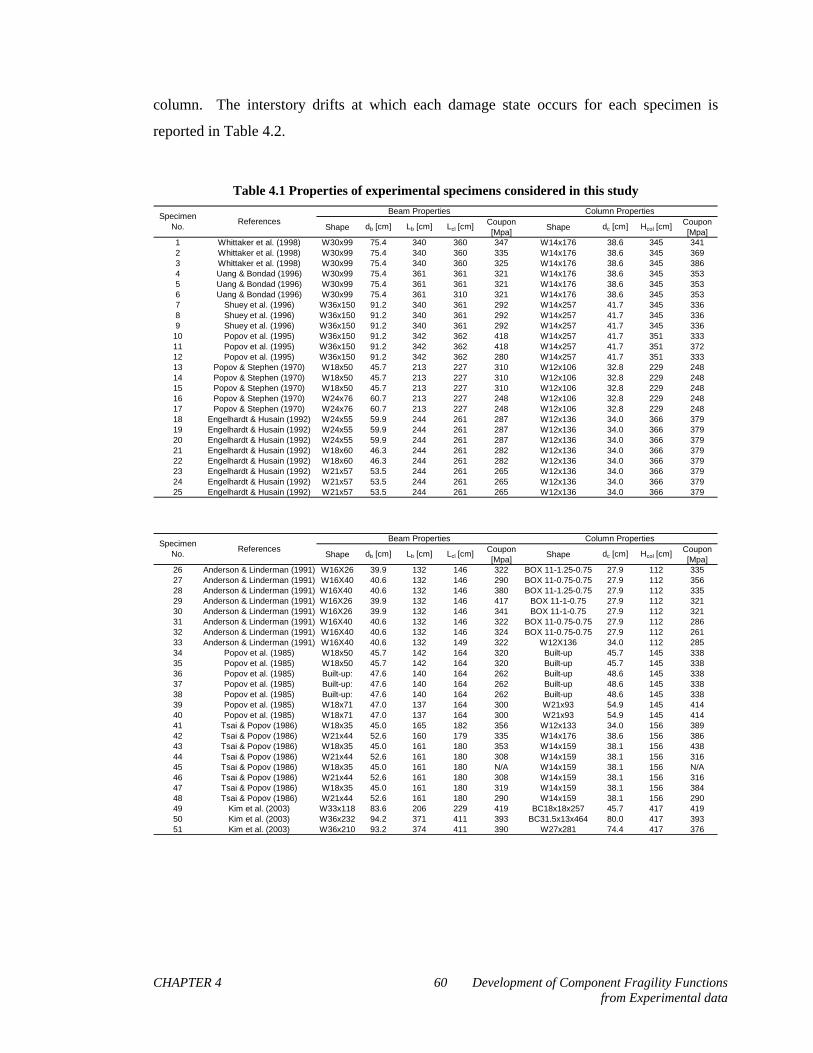
CHAPTER 4 60 Development of Component Fragility Functions from Experimental data
column. The interstory drifts at which each damage state occurs for each specimen is
reported in Table 4.2.
Table 4.1 Properties of experimental specimens considered in this study
Shape db [cm] Lb [cm] Lcl [cm] Coupon [Mpa]
Shape dc [cm] Hcol [cm] Coupon [Mpa]
1 Whittaker et al. (1998) W30x99 75.4 340 360 347 W14x176 38.6 345 3412 Whittaker et al. (1998) W30x99 75.4 340 360 335 W14x176 38.6 345 3693 Whittaker et al. (1998) W30x99 75.4 340 360 325 W14x176 38.6 345 3864 Uang & Bondad (1996) W30x99 75.4 361 361 321 W14x176 38.6 345 3535 Uang & Bondad (1996) W30x99 75.4 361 361 321 W14x176 38.6 345 3536 Uang & Bondad (1996) W30x99 75.4 361 310 321 W14x176 38.6 345 3537 Shuey et al. (1996) W36x150 91.2 340 361 292 W14x257 41.7 345 3368 Shuey et al. (1996) W36x150 91.2 340 361 292 W14x257 41.7 345 3369 Shuey et al. (1996) W36x150 91.2 340 361 292 W14x257 41.7 345 33610 Popov et al. (1995) W36x150 91.2 342 362 418 W14x257 41.7 351 33311 Popov et al. (1995) W36x150 91.2 342 362 418 W14x257 41.7 351 37212 Popov et al. (1995) W36x150 91.2 342 362 280 W14x257 41.7 351 33313 Popov & Stephen (1970) W18x50 45.7 213 227 310 W12x106 32.8 229 24814 Popov & Stephen (1970) W18x50 45.7 213 227 310 W12x106 32.8 229 24815 Popov & Stephen (1970) W18x50 45.7 213 227 310 W12x106 32.8 229 24816 Popov & Stephen (1970) W24x76 60.7 213 227 248 W12x106 32.8 229 24817 Popov & Stephen (1970) W24x76 60.7 213 227 248 W12x106 32.8 229 24818 Engelhardt & Husain (1992) W24x55 59.9 244 261 287 W12x136 34.0 366 37919 Engelhardt & Husain (1992) W24x55 59.9 244 261 287 W12x136 34.0 366 37920 Engelhardt & Husain (1992) W24x55 59.9 244 261 287 W12x136 34.0 366 37921 Engelhardt & Husain (1992) W18x60 46.3 244 261 282 W12x136 34.0 366 37922 Engelhardt & Husain (1992) W18x60 46.3 244 261 282 W12x136 34.0 366 37923 Engelhardt & Husain (1992) W21x57 53.5 244 261 265 W12x136 34.0 366 37924 Engelhardt & Husain (1992) W21x57 53.5 244 261 265 W12x136 34.0 366 37925 Engelhardt & Husain (1992) W21x57 53.5 244 261 265 W12x136 34.0 366 379
Beam Properties Column PropertiesSpecimen
No.References
Shape db [cm] Lb [cm] Lcl [cm] Coupon [Mpa]
Shape dc [cm] Hcol [cm] Coupon [Mpa]
26 Anderson & Linderman (1991) W16X26 39.9 132 146 322 BOX 11-1.25-0.75 27.9 112 33527 Anderson & Linderman (1991) W16X40 40.6 132 146 290 BOX 11-0.75-0.75 27.9 112 35628 Anderson & Linderman (1991) W16X40 40.6 132 146 380 BOX 11-1.25-0.75 27.9 112 33529 Anderson & Linderman (1991) W16X26 39.9 132 146 417 BOX 11-1-0.75 27.9 112 32130 Anderson & Linderman (1991) W16X26 39.9 132 146 341 BOX 11-1-0.75 27.9 112 32131 Anderson & Linderman (1991) W16X40 40.6 132 146 322 BOX 11-0.75-0.75 27.9 112 28632 Anderson & Linderman (1991) W16X40 40.6 132 146 324 BOX 11-0.75-0.75 27.9 112 26133 Anderson & Linderman (1991) W16X40 40.6 132 149 322 W12X136 34.0 112 28534 Popov et al. (1985) W18x50 45.7 142 164 320 Built-up 45.7 145 33835 Popov et al. (1985) W18x50 45.7 142 164 320 Built-up 45.7 145 33836 Popov et al. (1985) Built-up: 47.6 140 164 262 Built-up 48.6 145 33837 Popov et al. (1985) Built-up: 47.6 140 164 262 Built-up 48.6 145 33838 Popov et al. (1985) Built-up: 47.6 140 164 262 Built-up 48.6 145 33839 Popov et al. (1985) W18x71 47.0 137 164 300 W21x93 54.9 145 41440 Popov et al. (1985) W18x71 47.0 137 164 300 W21x93 54.9 145 41441 Tsai & Popov (1986) W18x35 45.0 165 182 356 W12x133 34.0 156 38942 Tsai & Popov (1986) W21x44 52.6 160 179 335 W14x176 38.6 156 38643 Tsai & Popov (1986) W18x35 45.0 161 180 353 W14x159 38.1 156 43844 Tsai & Popov (1986) W21x44 52.6 161 180 308 W14x159 38.1 156 31645 Tsai & Popov (1986) W18x35 45.0 161 180 N/A W14x159 38.1 156 N/A46 Tsai & Popov (1986) W21x44 52.6 161 180 308 W14x159 38.1 156 31647 Tsai & Popov (1986) W18x35 45.0 161 180 319 W14x159 38.1 156 38448 Tsai & Popov (1986) W21x44 52.6 161 180 290 W14x159 38.1 156 29049 Kim et al. (2003) W33x118 83.6 206 229 419 BC18x18x257 45.7 417 41950 Kim et al. (2003) W36x232 94.2 371 411 393 BC31.5x13x464 80.0 417 39351 Kim et al. (2003) W36x210 93.2 374 411 390 W27x281 74.4 417 376
Specimen No.
ReferencesBeam Properties Column Properties

CHAPTER 4 61 Development of Component Fragility Functions from Experimental data
Table 4.2 Interstory drifts at each damage state for each specimen
1 0.74 1.98 27 0.52 1.672 0.74 3.95 28 0.74 1.833 0.74 2.97 29 0.78 1.834 0.65 0.94 30 0.43 1.575 0.95 0.94 31 0.52 1.446 0.82 1.87 32 0.42 1.677 0.70 0.70 33 0.60 1.538 0.53 1.41 34 0.91 1.859 0.53 0.70 35 0.93 3.7110 0.55 2.10 36 0.56 2.1611 0.60 1.40 37 0.55 2.4712 0.63 2.10 38 0.57 2.0113 0.62 2.76 39 0.77 3.4914 0.61 3.65 40 0.74 3.8615 0.50 2.65 41 0.41 1.5016 0.56 4.90 42 0.51 1.2117 0.56 1.77 43 0.52 1.8418 0.73 1.17 44 0.43 2.5419 0.73 1.17 45 ** 0.4120 0.97 1.70 46 0.34 0.7721 0.97 1.07 47 0.33 1.9122 0.88 2.19 48 0.39 1.6523 0.97 1.95 49 0.75 0.7624 0.97 2.43 50 0.38 0.5925 0.88 1.95 51 0.38 0.5826 0.41 1.30
IDRDS1 [%] IDRDS2 [%]Specimen No.
IDRDS2 [%]IDRDS1 [%] Specimen No.
4.5 FRAGILITY FUNCTION FORMULATION
The data consolidated from the experimental studies listed in Table 4.2 was used to
develop drift-based fragility functions for yielding and fracture. As observed from Table
4.2, the interstory drift ratio at which the beam-column specimens reach these damage
states varies significantly from test to test. When estimating damage in existing WSMF
buildings built prior to 1994, it is important to account for this variability. Drift-based
fragility functions capture this specimen-to-specimen variability, providing a way of
estimating the probability that the joint will experience or exceed a particular damage state
given an imposed interstory drift demand. Fragility functions were created for each damage
state as described in the preceding sections.
CHAPTER 4 62 Development of Component Fragility Functions from Experimental data
Fragility functions are cumulative frequency distribution functions that provide the
variation of increasing probability of reaching or exceeding a damage state as interstory
drift increases. These functions are generated by first sorting the data, in ascending order,
by the interstory drift ratio at which the damage was reported for each damage state. These
values are then plotted against their cumulative probability of occurrence. In this study the
cumulative probability of occurrence was computed using the following equation:
( 0.5)i
Pn
(4.1)
where i is the position of the peak interstory drift ratio within the sorted data and n is the
number of specimens. This equation is also known as Hazen’s Model, and is one of several
commonly-used equations used to compute quantiles. This particular definition was
selected because previous research has shown this definition limits the amount of bias
introduced into the plotting position (Cunnane 1978). It also prevents the first data point in
a sample to be assigned a probability of 0 (i.e. the damage state will never occur at this
drift), and the last data point with a probability of 1 (i.e. the damage state is guaranteed to
occur at this drift), which is unrealistic. However, the differences between the different
definitions of the quantile are subtle and for large sample sizes, all of them converge to the
same value.
After the data is plotted, a lognormal cumulative distribution function was fitted to
the data points, by using its logarithmic statistical parameters to define the function. It has
been well-established that the lognormal distribution provides relatively good fit to
empirical cumulative distributions computed from experimental data (Aslani 2005; Aslani
and Miranda 2005; Pagni and Lowes 2006; Brown and Lowes 2007). The equation of this
fitted function is given by:
( ) ( )
( )iLnIDR
Ln idr Ln IDRP DS ds IDR idr
(4.2)

CHAPTER 4 63 Development of Component Fragility Functions from Experimental data
where P(DS ≥ dsi│IDR = idr) is the probability of experiencing or exceeding damage state
i, Ln IDR is the natural logarithm of the counted median of the interstory drift ratios
(IDRs) at which damage state i was observed, LnIDR is the standard deviation of the natural
logarithm of the IDRs, and is the cumulative standard normal distribution. Alternatively,
Ln IDR can be replaced by the geometric mean, which is the mean of the natural
logarithm of the data.
To ensure that the fitted functions are not skewed by outlying data points, outliers
were identified and removed from our fragilities. Chauvenet’s outlier criterion (Barnett
1978, Hawkins 1980, and Barnett and Lewis 1995), given by the following equations, was
used to determine whether or not the data points would be included:
1
2lowerpn
(4.3)
1
12upperp
n (4.4)
If a data point’s cumulative probability was smaller than the probability calculated with
Equation (4.3), or was greater than the probability calculated with Equation (4.4), then it
was excluded from the data set.
Kolmogorov-Smirnov goodness-of-fit tests (Benjamin and Cornell 1970) were
conducted to verify that the cumulative distribution function could be assumed to be
lognormally distributed. This was done by plotting graphical representations of this test for
10% significance levels on the same graph as the data and its fitted cumulative distribution
function. If all the data points lie within the bounded significance levels, the assumed
cumulative distribution function fits the empirical data adequately.
In addition to the specimen to specimen variability, statistical uncertainty was
considered to account for inherent uncertainty in the proposed fragility functions because
their parameters have been established using data with a limited amount of specimens
(finite-sample uncertainty). This uncertainty is quantified by bounding our fitted lognormal
cumulative distribution function with confidence intervals of the median and dispersion

CHAPTER 4 64 Development of Component Fragility Functions from Experimental data
parameters of IDR for each damage state. Conventional statistical methods can be used to
establish the confidence intervals because our underlying probability distribution is
lognormal. Crow et al. (1960) proposed the following equation to approximate the
confidence intervals of a lognormally distributed sample:
/ 2exp LnIDRIDR zn
(4.5)
where z/2 is the value in the standard normal distribution such that the probability of a
random deviation numerically greater than z/2 is , and n is the number of data points.
90% confidence intervals can were obtained and plotted for each fragility function.
4.5.1 Fragility Functions for Yielding
The experimental data used included specimens that were fabricated from both A36
and A572 grade 50 steel (Fy = 36 ksi and 50 ksi, respectively). The data was divided into
these two categories because the A36 specimens are expected to yield at lower drifts. It was
found that the difference in IDRs in the two groups was statistically significant. Therefore,
two separate fragility functions were created based on the yielding stress of the specimen.
When the test specimen consisted of members fabricated from differing types of steel (e.g.
the beam made from A36 and the column made from A572 grade 50), the specimen was
categorized based on the member where yielding first occurred. Figure 4.3a displays the
fragility function for test specimens whose yielded members were fabricated from A36
steel, while Figure 4.3b displays the fragility function for A572 grade 50 steel. Statistical
parameters for both functions are listed in Table 4.3.
Table 4.3 Uncorrected statistical parameters for IDRs corresponding to the damage states for Pre-Northridge beam-column joints

CHAPTER 4 65 Development of Component Fragility Functions from Experimental data
Damage StateMedian IDR
[%]Geometric Mean IDR LnIDR
Number of Specimens
(Outliers Removed)
DS1: YieldingA36: Uncorrected Raw Data 0.56 0.59 0.32 32A572: Uncorrected Raw Data 0.74 0.71 0.19 16
DS2: Fracture (Uncorrected) 1.85 1.79 0.47 50
DS = Yielding (A36)
0.0
0.2
0.4
0.6
0.8
1.0
0.0 0.5 1.0 1.5 2.0
Interstory Drift, IDR [%]
P(DS|IDR)
Data Fitted Curve K-S Test, 10% Signif.
(a)
DS = Yielding (A572)
0.0
0.2
0.4
0.6
0.8
1.0
0.0 0.5 1.0 1.5 2.0
Interstory Drift, IDR [%]
P(DS|IDR)
Data
Fitted Curve
K-S Test, 10% Signif.
(b)
Figure 4.3 Yielding without Correction for Span-to-Depth Ratio (a) A36 (b) A572 grade 50
CHAPTER 4 66 Development of Component Fragility Functions from Experimental data
Given an IDR, the fragility functions shown in Figure 4.3a and 3b can be used to
estimate the probability of experiencing yielding in pre-Northridge beam-column
connections. However, the accuracy of these predictions are dependent on whether the test
setups and member sizes of the experimental data used to create the fragility functions are
representative of the beam-to-column connections used in practice. Parameters that
strongly influence the IDR at which yielding occurs must be identified, to determine if their
values in the experimental data are representative of those used in practice. The influence
of various parameters was identified by plotting them against their corresponding IDR and
linear regression was conducted to develop relationships. A T-test (Benjamin and Cornell
1970) was used to determine which parameters statistically influenced the yielding IDR.
Test specimen parameters tested included beam depth, flange thickness and beam span-to-
depth ratio. Of these parameters, beam span-to-depth ratio was the only that exhibited
statistical significance based on the T-test criterion.
The relationship between span-to-depth ratio (L/db, where L, the centerline span of
the beam , is equal to 2*LcL) and the joint’s yielding IDR, was further investigated by
conducting linear regression on the two random variables. Figure 4.4a plots the natural
logarithm of the test specimens’ yielding IDR as a function the beam’s L/db for the A36
specimen. As shown in this figure, there is a clear trend that beams with small span-to-
depth ratios require less deflection/drift to initiate yielding in the beam-column joint. 95%
confidence intervals on the regressed linear trend computed from the data are also plotted in
the figure. The regression yields a significant correlation coefficient of 0.64, confirming the
statistical significance indicated by the T-test. The mean beam’s L/db for the A36 specimens
is 8.25, that corresponds to a median IDR of 0.56%. The trend between L/db and ln(IDR)
for the A572 grade 50 specimens is not as strong. The correlation coefficient in this case is
only 0.19. The mean L/db for the A572 grade 50 specimens is 8.0 at a corresponding
median IDR of 0.74%. The lower correlation of the A572 grade 50 specimens may be
largely due to the smaller sample size of experimental joints made from this type of steel,
but also due to the fact that in most A572 grade 50 specimens yielding was not initiated in
the beams but in the panel zones and therefore the beam’s L/db has a smaller influence.
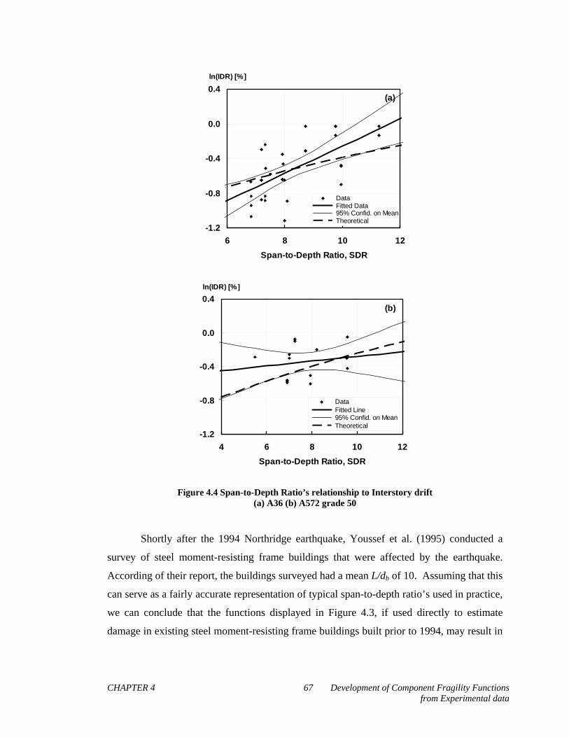
CHAPTER 4 67 Development of Component Fragility Functions from Experimental data
-1.2
-0.8
-0.4
0.0
0.4
6 8 10 12
Span-to-Depth Ratio, SDR
ln(IDR) [%]
Data Fitted Data95% Confid. on Mean Theoretical
(a)
-1.2
-0.8
-0.4
0.0
0.4
4 6 8 10 12
Span-to-Depth Ratio, SDR
ln(IDR) [%]
Data Fitted Line 95% Confid. on Mean Theoretical
(b)
Figure 4.4 Span-to-Depth Ratio’s relationship to Interstory drift (a) A36 (b) A572 grade 50
Shortly after the 1994 Northridge earthquake, Youssef et al. (1995) conducted a
survey of steel moment-resisting frame buildings that were affected by the earthquake.
According of their report, the buildings surveyed had a mean L/db of 10. Assuming that this
can serve as a fairly accurate representation of typical span-to-depth ratio’s used in practice,
we can conclude that the functions displayed in Figure 4.3, if used directly to estimate
damage in existing steel moment-resisting frame buildings built prior to 1994, may result in

CHAPTER 4 68 Development of Component Fragility Functions from Experimental data
underestimations of yielding IDR (which would lead to over predicting yielding), because
the test specimens used to develop these functions have a smaller span-to-depth ratios.
Table 4.4 Summary of Yousef et al.’s Building Survey Results for Typical Girder Sizes of Existing Buildings
d b Weighted Avg. L/d b Weighted Avg.(1) (2) (3) (4) (5) (6) (7) (8) (9) (10) (11)
W14/16 6 48 4.6 5.8 8.5 0.04 38 1.5 15.2 0.6W18 9 46 3.7 6.1 12.2 0.04 46 1.7 13.3 0.5W21 12 112 3.4 5.5 12.2 0.09 53 4.9 10.3 1.0W24 23 135 4 7 10.4 0.11 61 6.8 11.5 1.3W27 19 56 4.9 7.9 12.2 0.05 69 3.2 11.5 0.5W30 20 106 4 7.6 12.8 0.09 76 6.7 10.0 0.9W33 20 174 4.9 8.5 12.8 0.14 84 12.1 10.1 1.5W36 30 533 4.6 7.9 14 0.44 91 40.3 8.6 3.8
1210 77.2 10.0
Beam Depth [cm] Span-to-depth ratioWeight
Typical Girder
No of Bldgs
Floor-Frames
Min Bay [m]
Avg Bay [m]
Max Bay [m]
Notes:- Column (10) is the calculated average span-to-depth ratio calculated by dividing (5) by (8) accounting for unit conversion- A weighted average was used based on the number of floor frames included in Yousef et al.'s study. The weight (7) is found by taking the value of (3) and dividing it by the sum of column (3). For example, the weighted average for span-to-depth ratio is obtained by multiplying (7) by (10) to get (11), and then summing up column (11).
There are different alternatives approaches that one may use to modify the fragility
functions shown in Figure 4.3. A first approach is to compute the median IDR as a function
of the L/db ratio as follows:
exp[ ]bIDR a b L d (4.6)
where IDRy is the geometric mean IDR at yielding, and a and b are dimensionless
coefficients the y-intercept and the slope of the linear regression relationship respectively.
Table 4.5 documents the values of the regression coefficients, a and b, for the data
considered in this study for both A36 and A572 grade 50 specimens. In cases in which the
L/db ratio is not known, one could use an L/db of 10 (based on Yousef et al.’s survey), in
equation (4.6) and then the median IDRy become 0.77and 0.76 for A36 and A572 gr 50
specimens, respectively (see also Table 4.6). In cases where L/db is known, small
reductions in dispersion are achieved to 0.24 for A36 specimens and to 0.18 for A572 grade
50 specimens (Table 4.6).

CHAPTER 4 69 Development of Component Fragility Functions from Experimental data
DS = Yielding (A36)
0.0
0.2
0.4
0.6
0.8
1.0
0.0 0.5 1.0 1.5 2.0
Interstory Drift, IDR [%]
P(DS|IDR)
Original Function Corrected Function 90% Confid. Intervals
Figure 4.5 Recommended Fragility Function corrected for Span-to-Depth Ratio with 90% confidence bands
Table 4.5 Regression coefficients for relationship between IDRy and L/db
Regression Parameters
A36 Specimens
A572 Specimens
Y-intercept, a -1.83 -0.56Slope, b 0.16 0.028
Table 4.6 Recommended statistical parameters for fragility functions
Damage State
Information Available Type of Steel Median IDR [%] LnIDR
A36 0.77 0.32
A572 Gr. 50 0.76 0.19
A36 exp [-1.83 + 0.16*(L/d b )] 0.24
A572 Gr. 50 exp [-0.56 + 0.028*(L/d b )] 0.18
A36 1.42(IDR y ) 0.21
A572 Gr. 50 1.25(IDR y ) 0.32
DS1: Yielding
Only type of connection
Type of connection and L/d b
Type of connection and member data
A36 & A572 Gr. 50
1.85 0.47DS2:
FractureType of connection and d b
A36 & A572 Gr. 50
0.44exp [-0.99 + 0.0074*(d b )]
Only type of connection
Notes:L = centerline span = 2LcL
IDRy analytically computed insterstory drift at yieldingFor Fracture, there is no statistical difference with the type of steel.

CHAPTER 4 70 Development of Component Fragility Functions from Experimental data
Correction to account for different L/db ratios can also be done by deriving an
analytical expression of the IDR at yield as a function of L/db. Krawinkler et al. (2000)
derived equations that calculated IDRs for typical steel moment-resisting frame beam-
column connection test setups. In their approach, the IDR was computed as the sum of the
terms corresponding to three separate equations that represent the contributions of beam
flexure (IDRb), column flexure (IDRc), and panel zone shear (IDRPZ) as follows:
y b c PZIDR IDR IDR IDR (4.7)
where,
3
2
3
cdcL
bb cL
L PIDR
EI L
(4.8)
3
212b cL
cc
h d PLIDR
EI h
(4.9)
1 1b
PZs b
h d PLIDR
h A G d h
(4.10)
where P is the load imposed on the specimen, dc is the depth of the column, h is the height
of the column, Ic is the column’s moment of inertia, db is the depth of the beam, Ib is the
beam’s moment of inertia, L is the distance from the beam-end to the face of the column, E
is Young’s modulus and G is the corresponding shear modulus. Equations (4.7) to (4.10)
are only true under the following simplifying assumptions (Krawinkler et al. 2000): (i)
inflection points are assumed to occur at mid-height and at mid-span in columns and beams,
respectively; (ii) the is no vertical deflection in the point of inflection in the beam; (iii)
localized deformations in welds or slippage in bolted connections are ignored.

CHAPTER 4 71 Development of Component Fragility Functions from Experimental data
Assuming yielding will occur first in the beam we can express IDR due to beam
flexure in terms of the beam’s strain, y, and replace Equation (4.8) with:
2
13 2
c cLb y
cL b
d LIDR
L d
(4.11)
Then equations (4.8)-(4.10) can be re-written in terms of L/db as follows:
2
11
3 2yc
b bcL
FdIDR L d
L E
(4.12)
3
2212 c
yb bc bd
ccL
Fh d IIDR L d
I Eh L
(4.13)
2
22
2.6c
yb bPZ bd
c cb cL
Fh d IIDR L d
t d Eh d L
(4.14)
where Fy is the material yield stress and tc is the column’s web thickness. By using
equations (4.12)-(4.14) in equation (4.7) it is then possible to compute IDR at yield as a
function of L/db Table 4.7 displays mean values taken from our test specimens for the
parameters that are used in the derived analytical equations above. Figure 4.4a and b show
the analytical expression computed with these equation using the mean values indicated in
Table 4.7. It can be seen that, in both cases, the analytical expression falls within the 95%
confidence intervals suggesting that the linear regression of our data set follows the
analytical prediction.
Table 4.7 Average values for parameters in Equation (9), relating L/db and IDR

CHAPTER 4 72 Development of Component Fragility Functions from Experimental data
A36 Specimens
A572 Specimens
Beam PropertiesCoupon Yielding Stress, F y [Mpa] 310 352
Beam Depth, d b [cm] 54 66
Moment of Inertia, I b [cm 4 ] 79,084 145,681Span-to-depth ratio, SDR 8.25 7.91
Column PropertiesHeight of Column, h [cm] 234 264Column Depth, d c [cm] 34 44
Web Thickness, t c [cm] 2.4 2.2
Moment of Inertia, I c [cm] 59,937 90,322
Mean Values Parameters
In cases in which there is enough information (e.g., section geometry and nominal
material properties) to analytically compute the interstory drift at which yielding will be
initiated, then experimental information shown in Table 4.2 can be used to obtain a fragility
function specifically for each connection by considering a random variable , defined as the
ratio of the IDR in which yielding was observed in the test to the analytical yielding IDR as
follows:
Observed
y
IDR
IDR (4.15)
Figure 4.6 shows the cumulative distribution functions of for both the A36
specimens and the A572 grade 50 specimens. Figure 6 also shows fitted lognormal
distributions computed with parameters listed in Table 4.6 and 10% significance curves
corresponding to the Kolmogorov-Smirnov test, suggesting that the random variable can
also be assumed to be lognormally distributed.

CHAPTER 4 73 Development of Component Fragility Functions from Experimental data
for A36
0.0
0.2
0.4
0.6
0.8
1.0
0.0 1.0 2.0 3.0
Correction Factor,
P(DS | )
Data
Fitted Curve
K-S Test, 10%Significance
(a)
for A572
0.0
0.2
0.4
0.6
0.8
1.0
0.0 1.0 2.0 3.0
Correction Factor,
P(DS | )
Data
Fitted Curve
K-S Test, 10%Significance
(b)
Figure 4.6 Fragility Functions for to be used in conjunction with an analytical prediction of IDRy (a) A36 (b) A572 grade 50
For a given beam-to-column connection one would first compute analytically the
IDR corresponding to the onset of yielding and the median of the fragility function is then
computed as the product of IDRy and the median of Meanwhile the dispersion in the
fragility is set equal to the dispersion of shown in Table 4.6. It should be noted that using
this procedure a further reduction in dispersion was obtained for A36 specimens, however
for A572 grade 50 specimens the dispersion increased due to the fact that in several

CHAPTER 4 74 Development of Component Fragility Functions from Experimental data
specimens the location of yielding observed in the test was different to that predicted
analytically.
As an example of the latter approach, consider a pre-Northridge beam-to-column
connection between a W36x150 beam with a L/db ratio of 10 and W14x257 column both
made from A572 grade 50 steel. Using equations(4.7), (4.12), (4.13) and (4.14) one
computes IDRAnalytical =0.84 which considering the median and dispersion of shown in
table 6 results in the fragility function shown in Figure 4.7, which has a median of 1.05%
and logarithmic standard deviation of 0.32. Ninety percent confidence levels that account
for the statistical uncertainty are also shown in the figure.
A572
0.0
0.2
0.4
0.6
0.8
1.0
0.0 1.0 2.0 3.0
IDR [%]
P(DS|IDR)
Fitted Function
90% Confid. Intervals
Figure 4.7 Example Fragility Function for W36 beam generated by using (A572 grade 50)
4.5.2 Fragility Functions for Fracture
Fragility functions were also generated to estimate the probability of fracture as a
function of IDR. Unlike the yielding limit state in which an analytical prediction is possible
and therefore fragility functions were derived by using either a purely empirical approach
(i.e., entirely based on the experimental results) or by using a hybrid analytical-
experimental approach, for fracture there is not a reliable way to analytically estimate the
drift at which fracture is likely to occur in these connections, therefore in this case fragilities
were only based on experimental results. In the case of fracture the drifts at which A36
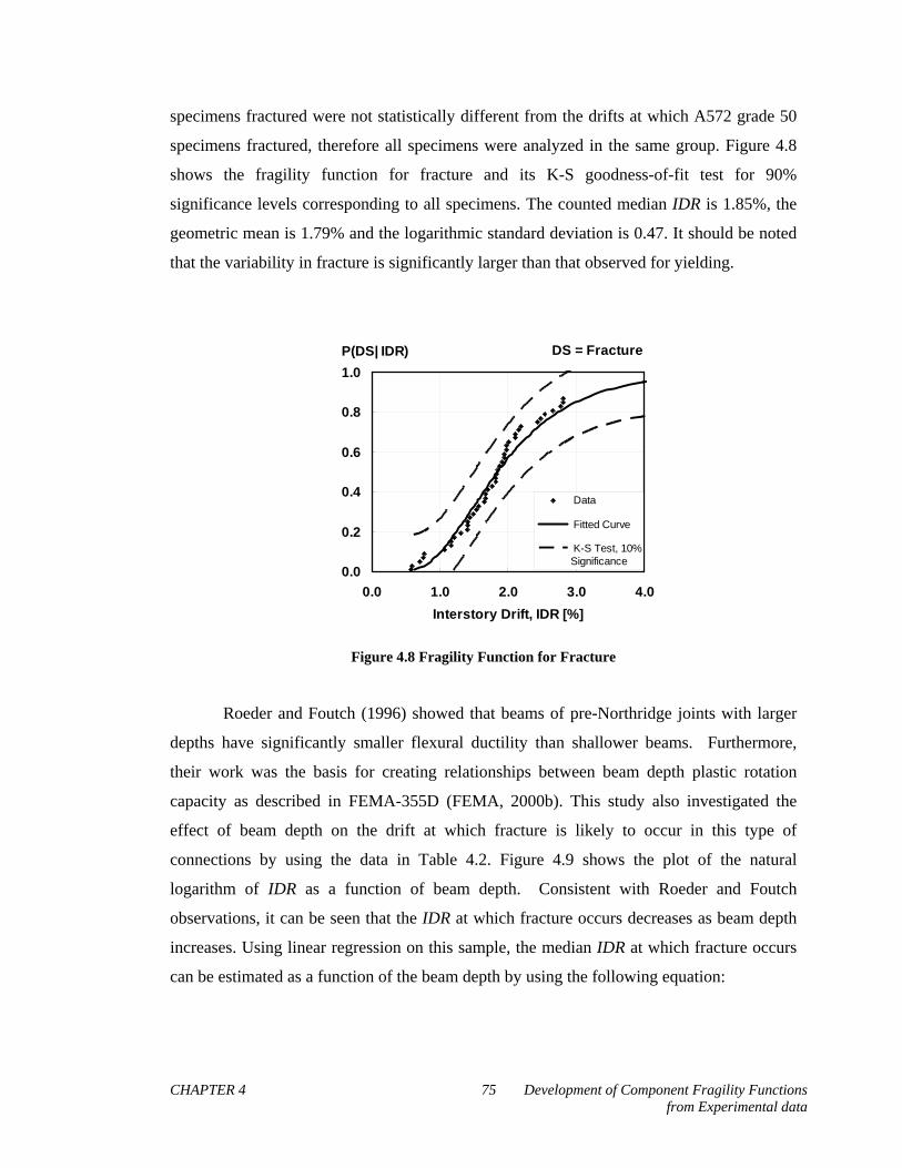
CHAPTER 4 75 Development of Component Fragility Functions from Experimental data
specimens fractured were not statistically different from the drifts at which A572 grade 50
specimens fractured, therefore all specimens were analyzed in the same group. Figure 4.8
shows the fragility function for fracture and its K-S goodness-of-fit test for 90%
significance levels corresponding to all specimens. The counted median IDR is 1.85%, the
geometric mean is 1.79% and the logarithmic standard deviation is 0.47. It should be noted
that the variability in fracture is significantly larger than that observed for yielding.
DS = Fracture
0.0
0.2
0.4
0.6
0.8
1.0
0.0 1.0 2.0 3.0 4.0
Interstory Drift, IDR [%]
P(DS| IDR)
Data
Fitted Curve
K-S Test, 10%Significance
Figure 4.8 Fragility Function for Fracture
Roeder and Foutch (1996) showed that beams of pre-Northridge joints with larger
depths have significantly smaller flexural ductility than shallower beams. Furthermore,
their work was the basis for creating relationships between beam depth plastic rotation
capacity as described in FEMA-355D (FEMA, 2000b). This study also investigated the
effect of beam depth on the drift at which fracture is likely to occur in this type of
connections by using the data in Table 4.2. Figure 4.9 shows the plot of the natural
logarithm of IDR as a function of beam depth. Consistent with Roeder and Foutch
observations, it can be seen that the IDR at which fracture occurs decreases as beam depth
increases. Using linear regression on this sample, the median IDR at which fracture occurs
can be estimated as a function of the beam depth by using the following equation:
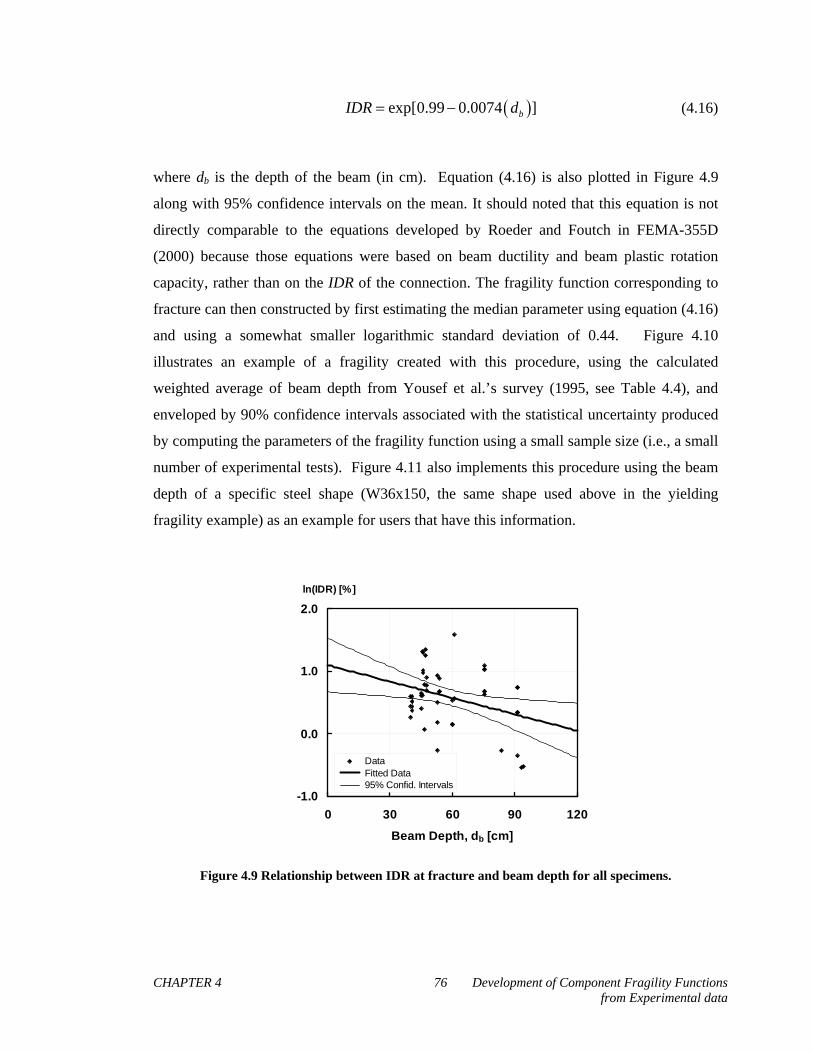
CHAPTER 4 76 Development of Component Fragility Functions from Experimental data
exp[0.99 0.0074 ]bIDR d (4.16)
where db is the depth of the beam (in cm). Equation (4.16) is also plotted in Figure 4.9
along with 95% confidence intervals on the mean. It should noted that this equation is not
directly comparable to the equations developed by Roeder and Foutch in FEMA-355D
(2000) because those equations were based on beam ductility and beam plastic rotation
capacity, rather than on the IDR of the connection. The fragility function corresponding to
fracture can then constructed by first estimating the median parameter using equation (4.16)
and using a somewhat smaller logarithmic standard deviation of 0.44. Figure 4.10
illustrates an example of a fragility created with this procedure, using the calculated
weighted average of beam depth from Yousef et al.’s survey (1995, see Table 4.4), and
enveloped by 90% confidence intervals associated with the statistical uncertainty produced
by computing the parameters of the fragility function using a small sample size (i.e., a small
number of experimental tests). Figure 4.11 also implements this procedure using the beam
depth of a specific steel shape (W36x150, the same shape used above in the yielding
fragility example) as an example for users that have this information.
-1.0
0.0
1.0
2.0
0 30 60 90 120
Beam Depth, db [cm]
ln(IDR) [%]
Data Fitted Data 95% Confid. Intervals
Figure 4.9 Relationship between IDR at fracture and beam depth for all specimens.
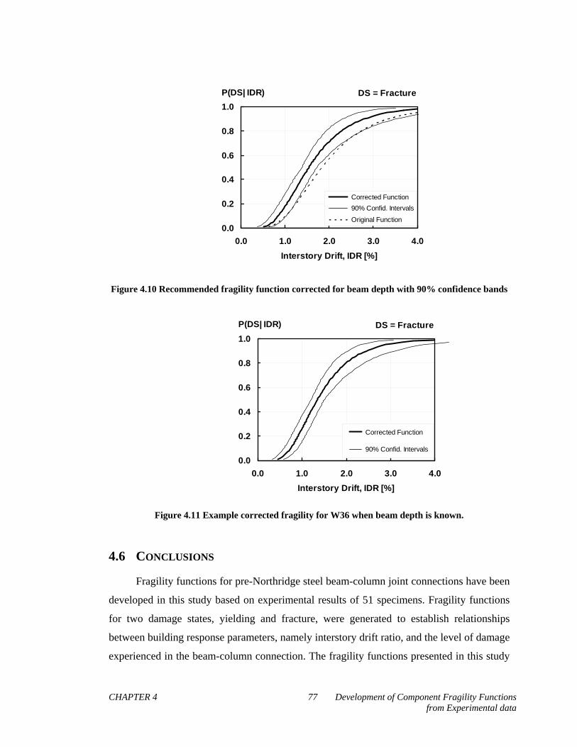
CHAPTER 4 77 Development of Component Fragility Functions from Experimental data
DS = Fracture
0.0
0.2
0.4
0.6
0.8
1.0
0.0 1.0 2.0 3.0 4.0
Interstory Drift, IDR [%]
P(DS| IDR)
Corrected Function
90% Confid. Intervals
Original Function
Figure 4.10 Recommended fragility function corrected for beam depth with 90% confidence bands
DS = Fracture
0.0
0.2
0.4
0.6
0.8
1.0
0.0 1.0 2.0 3.0 4.0
Interstory Drift, IDR [%]
P(DS| IDR)
Corrected Function
90% Confid. Intervals
Figure 4.11 Example corrected fragility for W36 when beam depth is known.
4.6 CONCLUSIONS
Fragility functions for pre-Northridge steel beam-column joint connections have been
developed in this study based on experimental results of 51 specimens. Fragility functions
for two damage states, yielding and fracture, were generated to establish relationships
between building response parameters, namely interstory drift ratio, and the level of damage
experienced in the beam-column connection. The fragility functions presented in this study

CHAPTER 4 78 Development of Component Fragility Functions from Experimental data
allow the incorporation of variability of deformation demands at which the two damage
states may occur. For the case of yielding three different sets of fragility functions were
developed. The first two fragility function employ a purely empirical approach in which the
parameters of the fragility function are computed with a span-to-depth ratio that
approximately represent those used in practice, or by using connection-specific span-to-
depth ratios. In the third fragility function uses a hybrid analytical-empirical approach in
which an analytical estimate of the drift at yielding is first computed and is then modified to
account for the bias and variability found using statistical information obtained between
observed and analytical drifts at yield for each specimen. Both empirical and hybrid
approaches indicate that the drift at which yielding is likely to occur increases with
increasing span-to-depth ratios, therefore consideration of the span-to-depth ratio when
estimating the likelihood of yielding does not only results in an improved estimate of the
median drift but also in a smaller dispersion. For the specimens considered in this study
analytical obtaining analytical predictions of the interstory drift at yield resulted in
insignificant further reduction in dispersion for A36 specimens and in an increment in
dispersion for A572 grade 50 specimens.
For estimating the probability of fracture only the empirical approach was used. It
was found that the drift at which fracture occurs decreases with increasing beam depths. For
beam depths between 76 and 91 cm (30 and 36 inches), which are commonly used in
practice in moment connections, median drifts that produce fracture in pre-Northridge
welded beam-to-column connections are between 1.47% and 1.31%, respectively.
Furthermore, the fragility functions developed in this study indicate that there is a
probability between 70% and 80% that WSMF buildings with pre-Northridge connections
experience fractures in their beam-to-column connections if they are subjected to interstory
drift demands of 2%, which is the maximum allowed in current U.S. codes in the design
level earthquake.
CHAPTER 5 79 Development of Component Fragility Functions from Empirical Data
CHAPTER 5
5 DEVELOPMENT OF COMPONENT FRAGILITY FUNCTIONS FROM EMPIRICAL DATA
This chapter is based on the following publication:
Ramirez, C.M., Cheong, K.F., Schrotenboer, T., and Miranda, E. (2008), Development of
Empirical Fragility Functions in Support of the Story-based loss estimation toolbox, Pacific
Earthquake Engineering Research Center Report, (in preparation).
5.1 AUTHORSHIP OF CHAPTER
Ramirez aided with developing the models used for structural analysis, computed the
fragility functions, and authored the publication. Cheong and Schrotenboer were
responsible for completing the analyses required to obtain the structural response
parameters. Miranda served as advisor and principal investigator for this project.
5.2 INTRODUCTION
Quantifying structural performance in terms of economic loss induced by seismic
ground motions requires estimating damage as a function of structural response. Fragility
functions compute the probability of being in to or exceeding a given damage state or
performance level as a function of a structural response parameter. Fragility functions need
to be assigned to all components in a building’s inventory to estimate the damage and
associated monetary loss that is representative of the entire value of the building. However,
functions for every type of building component are currently not available. Most studies
(see Chapter 2) on seismic-induced economic losses have ignored the loss due to
components without fragilities or accounted for their loss only when the structure collapsed

CHAPTER 5 80 Development of Component Fragility Functions from Empirical Data
(Goulet et al. 2007). Other investigators (Aslani and Miranda, 2005) have estimated the loss
in some of these components by using generic functions that were initially developed to be
used in regional methods (HAZUS) for some of these components. The data used to
develop these generic functions, however, are not well-documented and rely heavily on
expert opinion that has yet to be validated. Failing to account for economic losses due to
these types of components may lead to significant errors in the total estimated economic
loss and inaccurate projections of the loss’ composition. Until fragilities are available for all
building components, economic losses due to components without fragility functions need
to be accounted for in a reliable manner.
One way of accounting for these losses due to components without fragilities is using
generic fragility functions. Generic fragility functions are fragilities that are not component-
specific, but rather estimate the damage of groups of building components that are of the
same type. Components can be grouped into structural components and nonstructural
components for loss assessment purposes. Building components that do not have fragility
functions available can be grouped into these general categories and assigned these generic
fragilities such that their damage can be estimated collectively. Although damage estimated
from these functions may not be as precise as estimates generated from component-specific
functions, it yields better economic loss assessments than if the damage due to these
components is ignored.
Many generic fragility functions that are currently available are based on motion
damage relationships developed from expert opinion, such as those used in ATC-13 (ATC,
1985). Other functions, such as those used in HAZUS99 (FEMA, 1999), merge expert
opinion with analytical results. Empirical data collected after earthquakes have been used
to update these motion-damage relationships, however, the improvements made to these
models have been limited by the lack of relevant building performance data collected
(Anagnos et al., 1995, FEMA, 2000, Lizundia and Holmes, 1997). These empirical datasets
have been hampered by a variety of deficiencies, which include: small sample sizes that do
not provide enough data points, datasets that have a bias towards damaged or noteworthy
buildings, datasets that are limited by the amount of building types that are included,
datasets that are not collected in a consistent and complete manner, datasets that are
collected by private companies and are not available to the public and datasets that include
buildings that are not located close to free-field recording instruments (King et al., 2005).

CHAPTER 5 81 Development of Component Fragility Functions from Empirical Data
Recently, there have been efforts to improve the quality of empirical building
performance data. The ATC-38 project (ATC, 2000) conducted after the 1994 Northridge
earthquake attempted to systematically document the damage of buildings located near
locations of strong ground motion recording stations. Engineers inspected more than 500
buildings located within 1000 feet of 30 strong motion recording stations. As a result, a
thorough non-proprietary database now exists that includes the building properties and
damage performance, photos, and strong motion recordings. Degenkolb Engineers (Heintz
and Poland, 2001) also developed a similar database from an investigation conducted in
Taiwan after the 1999 Chi-Chi earthquake.
King et al. (2005) developed motion-damage relationships using the ATC-38 project
and other similar datasets to create lognormal fragility curves and damage probability
matrices. Spectral acceleration and interstory drift ratio, the latter estimated by using
spectral displacement and using a method proposed by Miranda (Miranda, 2000), were used
as structural response parameters to develop these fragility functions. Unfortunately, these
response parameters are based on single-degree of freedom systems that neglect the
contribution of higher mode effects and assume the structure is first mode dominated. This
may lead to inaccuracies in economic loss estimates for components that are damaged by
floor accelerations (acceleration-sensitive components) because floor accelerations are
strongly dependent on higher mode effects even in buildings with moderate heights. Even in
a first mode dominated structure, the building’s roof acceleration could be 20% to 60%
higher than the spectral acceleration because spectral acceleration is not equivalent to its
peak floor accelerations. Additionally, King et al. (2005) computed both spectral
accelerations and spectral displacements using approximations of the structural fundamental
period used in US building codes (ICC, 2003) with parameters proposed by Goel and
Chopra (1997). The equations used to approximate the fundamental period are not building-
specific and may lead to inaccurate estimations of interstory drift ratios.
This study is primarily aimed at obtaining generic fragility functions for nonstructural
components where there is very scarce information. Of particular interest is to obtain
information about the levels of structural response which trigger nonstructural damage since
this information is particularly important when computing expected annualized losses
(EALs). This study also attempts to improve the way empirical generic fragility functions
are developed by capturing structural response using better response parameters and more
advanced methods of structural simulation to estimate these parameters. Instead of using

CHAPTER 5 82 Development of Component Fragility Functions from Empirical Data
spectral acceleration and spectral displacement as response parameters, floor accelerations
and interstory drift ratios computed from analyses that model multi-degree of freedom
systems are used. Two sets of buildings that had damage data collected and documented
after the 1994 Northridge earthquake were modeled. The first set of data was extracted from
19 instrumented buildings established the California Strong Motion Instrumentation
Program (CSMIP). The responses of these buildings were computed using a continuous
model developed by Miranda (1999) that has been shown to approximate floor accelerations
and interstory drift ratios relatively well (Miranda, 1999; Miranda and Taghavi, 2005). The
response parameters computed from the continuous model were validated using the
response data recorded by the accelerographs contained in these buildings. The second set
of data was taken from the ATC-38 report (ATC, 2000). These buildings were not
instrumented but because they were located close to ground motion recording stations, the
ground motions recorded at these stations can be used in structural simulation to estimate
what the peak structural response parameters were during this earthquake. A probabilistic
approach using Monte Carlo simulation was used to obtain the most probable values of the
response parameters. Once the response parameters were established, they were paired with
the reported damage states for different groups of building components to create motion-
damage pairs. The motion-damage pairs were used to create fragility functions. These
fragility functions were then used to estimate damage for building components without
component-specific fragilities in Chapter 3 of this dissertation to develop EDP-DV
functions that relate structural response directly to monetary loss and used as part of the
Pacific Earthquake Engineering Research (PEER) center’s loss estimation toolbox, detailed
in Chapter 6.
5.3 SOURCES OF EMPIRICAL DATA
5.3.1 Instrumented Buildings (CSMIP)
The California Strong Motion Instrumentation Program (CSMIP) was established in
1972 to gather seismic activity data by instituting a network of accelerographs throughout
the state. The network includes 170 instrumented buildings, 19 of which have damage
documented during the 1994 Northridge Earthquake. For every building, a brief description
of the structure was provided which included several structural characteristics. A summary

CHAPTER 5 83 Development of Component Fragility Functions from Empirical Data
of these building properties is listed in Table 5.1. These characteristics included the
building’s number of stories, occupancy type and type of lateral force resisting system. The
building’s location in terms of latitude and longitude is reported and in particular its
distance to the earthquake’s epicenter. Sensors are located throughout each building on the
ground floor and selected floors above ground. Each sensor recorded accelerations during
the Northridge earthquake.
Table 5.1 CSMIP Building Properties
Station IDNo. of Stories
Lateral Resisting System
Occupancy TypeDist. To
Epicenter [km]
Interstory Ht. [cm]
EQ Direction
Period [s] AlphaDamping
Ratio
24231 7 Steel MRF School 18 411 EW 1.10 4.1 0.05424231 7 Steel MRF School 18 411 NS 0.62 7.0 0.10024236 14 Rconcrete MRF Warehouse 23 320 EW 0.81 8.5 0.08824236 14 Rconcrete MRF Warehouse 23 320 NS 2.30 5.0 0.07524322 13 Rconcrete MRF Commercial 9 358 EW 2.92 29.5 0.05024322 13 Rconcrete MRF Commercial 9 358 NS 2.60 19.1 0.09024332 3 Shear Walls Commercial 20 508 EW 0.48 6.0 0.03524332 3 Shear Walls Commercial 20 508 NS 0.59 30.0 0.05024370 6 SMRF Commercial 22 396 EW 1.39 30.0 0.04024370 6 SMRF Commercial 22 396 NS 1.38 30.0 0.02924385 10 Shear Walls Residential 21 207 EW 0.59 2.0 0.05524385 10 Shear Walls Residential 21 207 NS 0.60 2.0 0.05924386 7 Rconcrete MRF Hotel 7 265 EW 1.98 8.9 0.13024386 7 Rconcrete MRF Hotel 7 265 NS 1.60 5.0 0.13024463 5 Rconcrete MRF Warehouse 36 725 EW 1.45 10.2 0.03724463 5 Rconcrete MRF Warehouse 36 725 NS 1.62 15.5 0.03524464 20 Rconcrete MRF Hotel 19 257 EW 2.60 9.1 0.05024464 20 Rconcrete MRF Hotel 19 257 NS 2.79 29.0 0.03024514 6 Shear Walls Hospital 16 472 EW 0.30 3.5 0.18024514 6 Shear Walls Hospital 16 472 NS 0.37 3.0 0.18024579 9 Rconcrete MRF Office Building 32 396 EW 1.29 4.1 0.05324579 9 Rconcrete MRF Office Building 32 396 NS 1.04 29.5 0.05024580 2 Base Isolation Office Building 38 NA NA NA NA NA24580 2 Base Isolation Office Building 38 NA NA NA NA NA24601 17 Shear Walls Residential 32 264 EW 1.08 1.8 0.03324601 17 Shear Walls Residential 32 264 NS 1.14 1.5 0.03624602 52 Steel MRF Office Building 31 396 EW 6.20 6.9 0.01524602 52 Steel MRF Office Building 31 396 NS 5.90 9.8 0.01024605 7 Base Isolation Hospital 36 NA NA NA NA NA24605 7 Base Isolation Hospital 36 NA NA NA NA NA24629 54 Steel MRF Office Building 32 396 EW 5.60 30.0 0.00524629 54 Steel MRF Office Building 32 396 NS 6.20 27.5 0.00924643 19 Steel MRF Office Building 20 406 EW 3.90 30.0 0.02124643 19 Steel MRF Office Building 20 406 NS 3.47 4.0 0.02624652 6 Steel MRF Office Building 31 427 EW 0.91 30.0 0.04924652 6 Steel MRF Office Building 31 427 NS 0.86 13.0 0.03224655 6 Steel MRF Parking Structure 31 305 EW 0.40 1.4 0.06724655 6 Steel MRF Parking Structure 31 305 NS 0.51 2.0 0.102
The damage collected for each building used the criteria established by ATC-13
(ATC, 1985). Overall damage for the entire building was reported using the following
damage states: none, insignificant, moderate and heavy. These damage states are defined in
Table 5.2. In addition to the reporting the building’s overall damage, damage to specific

CHAPTER 5 84 Development of Component Fragility Functions from Empirical Data
components of the structure was evaluated. Damage experienced by the buildings’
structural components, its nonstructural components, its equipment and its contents were
also documented. Seven damage states, defined in Table 5.3, for each sub-category was
used to measure the performance of each component group. The economic loss associated
with each damage state was expressed as a percentage of the replacement cost of the group
of components.
Table 5.2 General Damage Classifications (ATC-13, 1985)
Code Description
N None . No damage is visible, either structural or non-structural
I
Insignificant. Damage requires no more than cosmetic repair. No structural repairs are necessary. For non-structural elements this would include spackling partition cracks, picking up spilled contents, putting back fallen ceiling tiles, and righting equipement.
M
Moderate. Repairable structural damage has occurred. The existing elements can be repaired in place, without substantial demolition or replacement or elements. For non-structural elements this would include minor replacement of damaged partitions, ceilings, contents or equipment.
H
Heavy. Damage is so extensive that repair of elements is either not feasible or requires major demolition or replacement. For non-structural elements this would include major or complete replacement of damaged partitions, ceilings, contents or equipment.
Table 5.3 ATC-13 Damages States (ATC, 1985)
State Description Percent Damage
1 None 0%2 Slight 0% - 1%3 Light 1% - 10%4 Moderate 10% - 30%5 Heavy 30% - 60%6 Major 60% - 100%7 Destroyed 100%
5.3.2 Buildings surveyed in the ATC-38 Report
ATC-38 was conducted to collect data that would improve motion-damage
relationships for earthquake damage and loss modeling. During the days after the 1994
Northridge earthquake the Applied Technology Council (ATC), the United States
Geological Survey (USGS) and other Northern California organizations concerned with

CHAPTER 5 85 Development of Component Fragility Functions from Empirical Data
earthquake engineering systematically documented building performance of structures
located within 300 meters (~1000 feet) of strong ground motion recording stations. 530
buildings near 31 recording stations were surveyed during the study. Eighteen of the
stations are operated by the California Division of Mines and Geology (CDMG), 7 are
operated by the University of Southern California (USC), and 6 are operated by USGS.
Digitized strong motion recordings were collected.
Standardized survey forms were used to evaluate the buildings and collect key
information. The buildings were categorized by their occupancy type as reported in Table
5.4. Photographs were taken to document the size, shape and visible damage. The survey
documented important structural characteristics for each building such as its design date,
predominant structural framing type (as defined by ATC, see Table 5.5), occupancy type
and number stories. The building’s nonstructural characteristics, equipment and contents
were also recorded. Building performance was evaluated by recording the degree of damage
experienced by the structural system, nonstructural components, equipment and contents.
Damage was measured using the same criteria established by ATC-13 and used for the
instrumented buildings described in Section 5.3.1.
Table 5.4 Occupancy Types and Codes (ATC-38)
Occupancy Type Refence Code
Apartment AAuto Repair ARChurch CDwelling DData Center DCGarage GGas Station GSGovernment GVHospital HHotel HLManufacturing MOffice ORestaurant RRetail RSSchool STheater TUtility UWarehouse WOther OTHUnknown UNK

CHAPTER 5 86 Development of Component Fragility Functions from Empirical Data
Table 5.5 Model Building Types (ATC-38)
Framing System
Steel Moment Frame S1 - Stiff Diaphragms S1A - Flexible DiaphragmsSteel Braced Frame S2 - Stiff Diaphragms S2A - Flexible DiaphragmsSteel Light FrameSteel Frame w/ Concrete Shear Walls S4 - Stiff Diaphragms S4A - Flexible DiaphragmsSteel Frame w/ Infill Masonry Shear Walls S5 - Stiff Diaphragms S5A - Flexible DiaphragmsConcrete Moment Frame C1 - Stiff Diaphragms C1A - Flexible DiaphragmsConcrete Shear Wall Building C2 - Stiff Diaphragms C2A - Flexible DiaphragmsConcrete Frame w/ Infill Masonry Shear Walls C3 - Stiff Diaphragms C3A - Flexible DiaphragmsReinforced Masonry Bearing Wall RM1 - Flexible Diaphragms RM2 - Stiff DiaphragmsUnreinforced Masonry Bearing Wall URM - Flexible Diaphragms URMA - Stiff DiaphragmsPrecast/Tiltup Concrete Shear Walls PC1 - Flexible Diaphragms PC1A - Stiff DiaphragmsPrecast Concrete Frame w/ Concrete Shear WallsWood Light FrameCommercial or Long-Span Wood Frame W2
Reference Codes and Diaphragm Types
PC2
S3
W1
5.4 DATA FROM INSTRUMENTED BUILDINGS
5.4.1 Structural response simulation
The response parameters being considered in this study to create fragility functions
are listed and defined as the following:
Peak Building Acceleration (PBA): The maximum acceleration
experienced by the building at any floor during the earthquake.
Peak Interstory Drift (IDR): The maximum interstory drift experienced
by the building at any story during the earthquake
These response parameters are also often referred to as engineering demand
parameters (EDPs) under the terminology established by PEER for their performance-based
earthquake engineering framework (Krawinkler and Miranda, 2004). Calculating these
parameters requires knowing what the maximum displacements and accelerations are for
every floor of each building. The sensors for each CSMIP building were not located at
every floor. Therefore, approximate methods of structural analysis were used to evaluate the
building’s response at the intermediate floors that did not have any motion recordings.
Taghavi and Miranda (2005) have shown that in many cases it is possible to obtain
a relatively good approximation of the response of buildings subjected to earthquake ground
motions. In their model, the building is replaced by a continuous system consisting of a
shear beam laterally connected to a flexural beam by axially ridge struts (Figure 5.1). The
continuous system’s primary advantage is that it requires only three parameters to calculate

CHAPTER 5 87 Development of Component Fragility Functions from Empirical Data
the dynamic properties of the structure: the building’s fundamental period of vibration, its
damping ratio and a non-dimensional parameter, 0, which controls the degree of flexural
or shear deformation. Closed-form solutions solving the dynamic equation of motion for the
continuous system were derived that compute the considered building’s mode shapes, its
corresponding modal participation factors and period ratio. Once the considered structure’s
dynamic characteristics have been determined, they can be used in combination with
traditional time-integration schemes to evaluate the structural response when subjected to
seismic ground accelerations.
H
Shear beam
Flexuralbeam
Axially-rigid links
H
Shear beam
Flexuralbeam
Axially-rigid links
Figure 5.1 Continuous Model used to evaluate structural response
The distribution of the building mass and stiffness was assumed to be uniform along
the height of the structure. Although making this assumption may seem restrictive, Miranda
and Taghavi (2005) have shown that, provided that there are no large sudden changes in
mass or stiffness along the height, this model leads to reasonable approximations of the
dynamic characteristics of many types of buildings. Any deviation in response that was
produced by nonuniform mass or stiffness, was small enough to neglect or could be
accounted for by using approximate equations.
The continuous model has been shown to have produced similar structural
responses for structures responding elastically that were predicted by more rigorous models
that required greater computational effort. Furthermore, by using the building’s
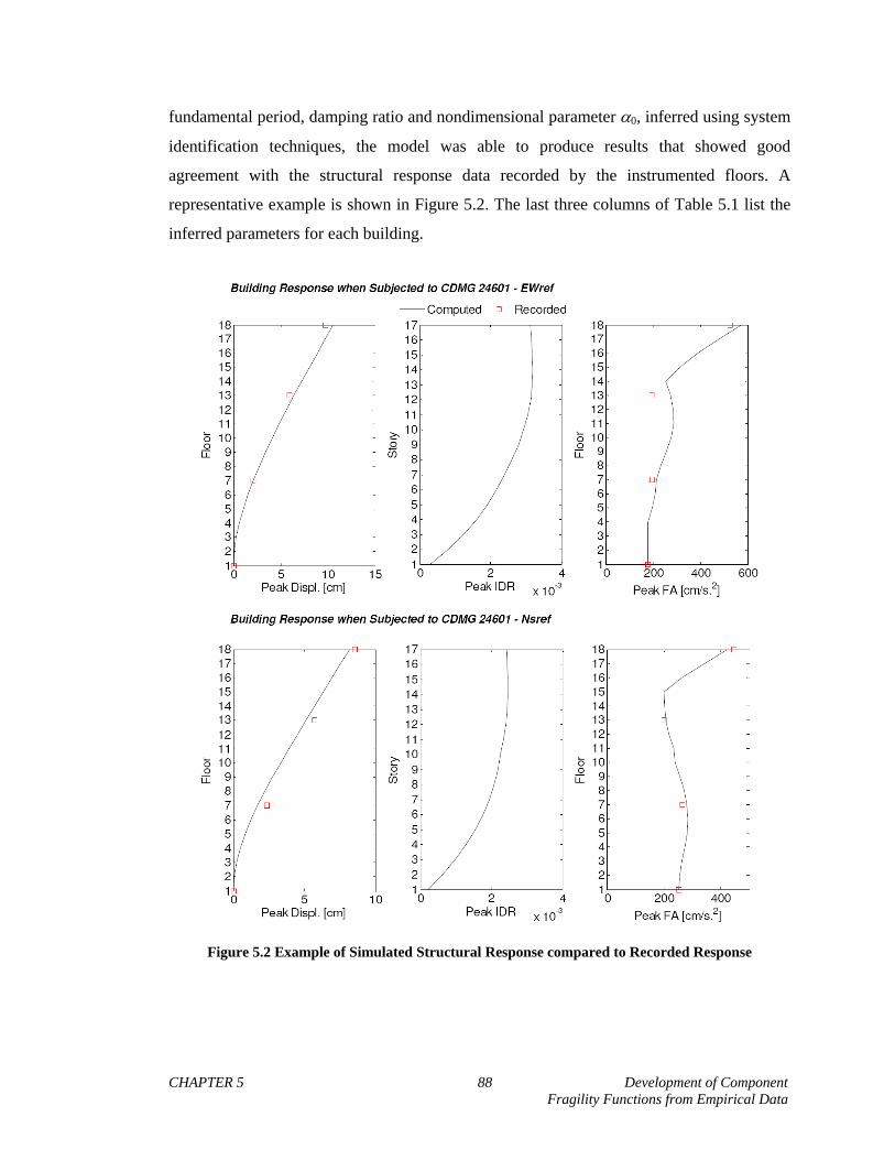
CHAPTER 5 88 Development of Component Fragility Functions from Empirical Data
fundamental period, damping ratio and nondimensional parameter 0, inferred using system
identification techniques, the model was able to produce results that showed good
agreement with the structural response data recorded by the instrumented floors. A
representative example is shown in Figure 5.2. The last three columns of Table 5.1 list the
inferred parameters for each building.
Figure 5.2 Example of Simulated Structural Response compared to Recorded Response
CHAPTER 5 89 Development of Component Fragility Functions from Empirical Data
Detailed summary sheets comparing how well each of the 19 instrumented
buildings’ simulated response matched its recorded response were complied. The computed
peak floor acceleration, the floor acceleration spectra, the floor acceleration and
displacement response histories are compared to those recorded by the buildings’ sensors.
An example of the type of data reported is shown in Figure 5.3.

CHAPTER 5 90 Development of Component Fragility Functions from Empirical Data
Figure 5.3 CSMIP Building Response Comparison Summary Sheet Layout

CHAPTER 5 91 Development of Component Fragility Functions from Empirical Data
Figure 5.3 CSMIP Building Response Comparison Summary Sheet Layout (cont.)
CHAPTER 5 92 Development of Component Fragility Functions from Empirical Data
5.4.2 Motion-damage pairs for each building
Summary sheets were assembled to consolidate all the structural response and
damage information gathered for each of the 19 instrumented CSMIP buildings included in
this study. Figure 5.4 illustrates an example of the type of data generated for each building.
The example building shown is a 17 story shear wall residential building. General building
characteristics (e.g. number of stories, type of lateral resisting system, occupancy
type…etc) and a summary of the reported damage are documented. A map showing the
locations of the sensors in each building and plots of peak response parameters, similar to
those shown in Figure 5.2, are also reported in the summary sheets.
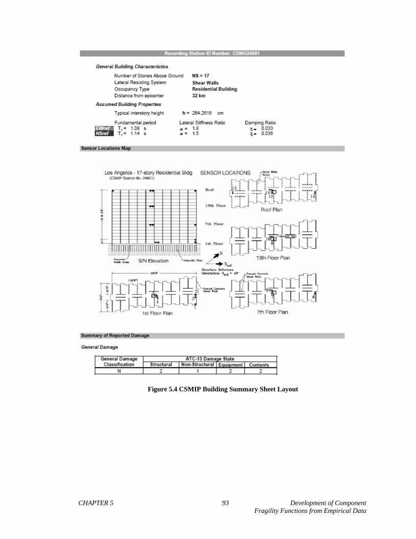
CHAPTER 5 93 Development of Component Fragility Functions from Empirical Data
Figure 5.4 CSMIP Building Summary Sheet Layout

CHAPTER 5 94 Development of Component Fragility Functions from Empirical Data
Figure 5.4 CSMIP Building Summary Sheet Layout (cont.)
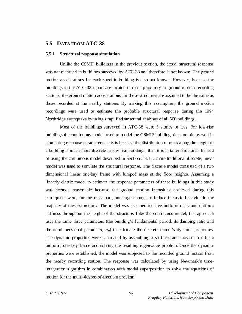
CHAPTER 5 95 Development of Component Fragility Functions from Empirical Data
5.5 DATA FROM ATC-38
5.5.1 Structural response simulation
Unlike the CSMIP buildings in the previous section, the actual structural response
was not recorded in buildings surveyed by ATC-38 and therefore is not known. The ground
motion accelerations for each specific building is also not known. However, because the
buildings in the ATC-38 report are located in close proximity to ground motion recording
stations, the ground motion accelerations for these structures are assumed to be the same as
those recorded at the nearby stations. By making this assumption, the ground motion
recordings were used to estimate the probable structural response during the 1994
Northridge earthquake by using simplified structural analyses of all 500 buildings.
Most of the buildings surveyed in ATC-38 were 5 stories or less. For low-rise
buildings the continuous model, used to model the CSMIP building, does not do as well in
simulating response parameters. This is because the distribution of mass along the height of
a building is much more discrete in low-rise buildings, than it is in taller structures. Instead
of using the continuous model described in Section 5.4.1, a more traditional discrete, linear
model was used to simulate the structural response. The discrete model consisted of a two
dimensional linear one-bay frame with lumped mass at the floor heights. Assuming a
linearly elastic model to estimate the response parameters of these buildings in this study
was deemed reasonable because the ground motion intensities observed during this
earthquake were, for the most part, not large enough to induce inelastic behavior in the
majority of these structures. The model was assumed to have uniform mass and uniform
stiffness throughout the height of the structure. Like the continuous model, this approach
uses the same three parameters (the building’s fundamental period, its damping ratio and
the nondimensional parameter, 0) to calculate the discrete model’s dynamic properties.
The dynamic properties were calculated by assembling a stiffness and mass matrix for a
uniform, one bay frame and solving the resulting eigenvalue problem. Once the dynamic
properties were established, the model was subjected to the recorded ground motion from
the nearby recording station. The response was calculated by using Newmark’s time-
integration algorithm in combination with modal superposition to solve the equations of
motion for the multi-degree-of-freedom problem.

CHAPTER 5 96 Development of Component Fragility Functions from Empirical Data
The fundamental period, damping ratio and nondimensional parameter 0 for each
building reported in ATC-38 is not known because the buildings were not instrumented.
Therefore, instead of computing only one solution through a deterministic approach, a
probabilistic method of estimating each building’s structure properties and corresponding
response was used to account for modeling uncertainty. Each building’s fundamental
period, damping ratio and parameter 0 were treated as independent random variables that
were lognormally distributed. A lognormal distribution was assumed because realizations of
this distribution can not be less than or equal to zero and some studies have shown to be
appropriate for the fundamental period and damping ratios.
The median and dispersion of each random variable were estimated using formulas
determined for twelve general model building types, shown in Table 5.6. After defining
these probability distributions, Monte Carlo methods were used to generate 200 different
realizations with combinations of the random variables. Each combination of building
parameters was used together with an assumed interstory height (also found in Table 5.6) as
input to define the discrete model. A time history analysis was conducted using the nearby
recorded ground motion to simulate the building’s response in terms of the parameters
defined in Section 5.4.1. Statistical analysis was then conducted on the results of the 200
simulations to establish the median (50th percentile) and dispersion (15th and 85th
percentiles) of the simulations. The response was computed for each directional component
of the recorded ground acceleration producing response results in both component
directions. In order to find a numerical average for the predicted motions, the geometric
mean was calculated from the two component directions. Figure 5.5 displays an example of
the results for the simulated structural response of one of the ATC-38 buildings. Each graph
plots the three response parameters along the height of the building and displays the results
of all 200 simulations, with the 15th, 50th, and 85th percentiles highlighted

CHAPTER 5 97 Development of Component Fragility Functions from Empirical Data
Table 5.6 Formulas used for Estimating Structural Building Parameters
Predominant MBT Typical
Interstory
Height
[ft]
Period Alpha Damping Ratio
Code Description
Median,
1T
Dispersion
Parameter,
1T
Median,
Dispersion
Parameter,
Median,
Dispersion
Parameter,
S1,
S1A
Steel Moment Resisting
Frame 13.75 0.035H 0.805 0.3 25 0.2 0.1057NS -0.565 0.40
S2,
S2A Steel Brace Frame 13.75 0.017H 0.9 0.3 6 0.2 0.03 0.35
S3 Steel Light Frame 13.0 0.038H 0.8 0.3 20 0.2 0.1057NS -0.565 0.35
S4,
S4A
Steel Frame w/
Concrete Shear Walls 13.75 0.017H 0.9 0.3 10 0.2 0.03 0.35
S5,
S5A
Steel Frame w/ Infill
Masonry Shear Wall 13.75 0.023H 0.85 0.3 18 0.2 0.04 0.35
RM1,
RM2,
URM,
URMA
Masonry Buildings 12.0 0.017H 0.3 5 0.2 0.278NS -0.701 0.20
C1,
C1A
RC Moment Resisting
Frame
9.0 – res., hotel
13.8 – other 0.017H 0.92 0.3 25 0.2 0.0889NS -0.235 0.20
C2,
C2A
Concrete Shear Wall
12.45 0.0069H 0.3 3 0.2 0.0889NS -0.235 0.30
C3,
C3A
Concrete Frame w/
Infill Masonry Shear
Wall
9.0 – res., hotel
13.8 – other 0.015H 0.9 0.3 18 0.2 0.09NS -0.24 0.25
PC1,
PC1A
Precast/Tiltup Concrete
Shear Wall 16.0 0.007H 0.3 3 0.2 0.06 0.30
W1 Wood Light Frame
Buildings 10.0 0.032H 0.55 0.3 7 0.2 0.077 0.40
W2
Commercial Wood
Frame Buildings
(Longspan)
13.4 0.032H 0.55 0.3 15 0.2 0.077 0.40
NOTE: H = height of building [ft] ( = typical interstory height [ft] * number of stories )
NS = number of stories above ground
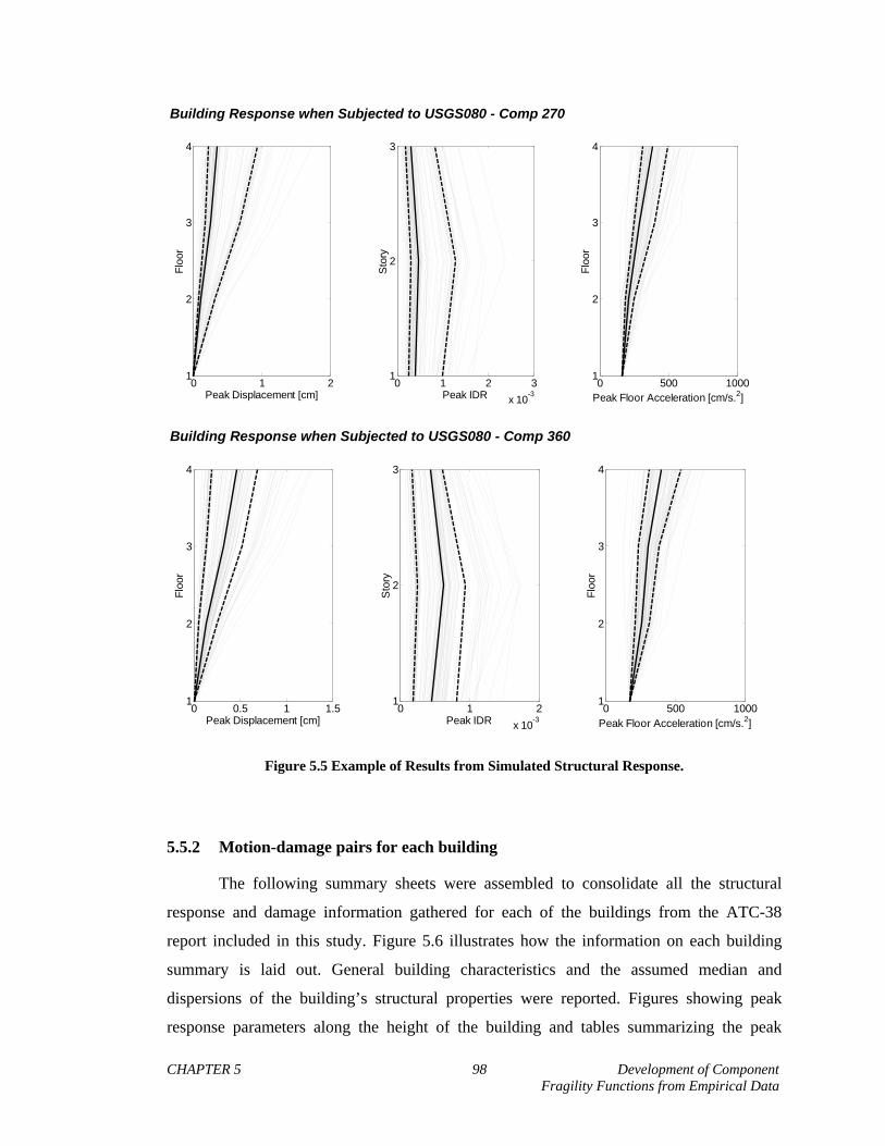
CHAPTER 5 98 Development of Component Fragility Functions from Empirical Data
Building Response when Subjected to USGS080 - Comp 270
0 1 21
2
3
4
Peak Displacement [cm]
Flo
or
0 1 2 3
x 10-3
1
2
3
Peak IDRS
tory
0 500 10001
2
3
4
Peak Floor Acceleration [cm/s.2]
Flo
or
Building Response when Subjected to USGS080 - Comp 360
0 0.5 1 1.51
2
3
4
Peak Displacement [cm]
Flo
or
0 1 2
x 10-3
1
2
3
Peak IDR
Sto
ry
0 500 10001
2
3
4
Peak Floor Acceleration [cm/s.2]
Flo
or
Figure 5.5 Example of Results from Simulated Structural Response.
5.5.2 Motion-damage pairs for each building
The following summary sheets were assembled to consolidate all the structural
response and damage information gathered for each of the buildings from the ATC-38
report included in this study. Figure 5.6 illustrates how the information on each building
summary is laid out. General building characteristics and the assumed median and
dispersions of the building’s structural properties were reported. Figures showing peak
response parameters along the height of the building and tables summarizing the peak

CHAPTER 5 99 Development of Component Fragility Functions from Empirical Data
response values, for each direction of ground motion component and the geometric mean of
the two components, are also documented. Lastly, a summary of the reported damage is
tabulated for both general damage and nonstructural damage of specific components.

CHAPTER 5 100 Development of Component Fragility Functions from Empirical Data
Figure 5.6 ATC-38 Building Summary Sheet Layout

CHAPTER 5 101 Development of Component Fragility Functions from Empirical Data
Figure 5.6 ATC-38 Building Summary Sheet Layout (cont.)

CHAPTER 5 102 Development of Component Fragility Functions from Empirical Data
5.6 FRAGILITY FUNCTIONS FORMULATION
5.6.1 Procedures to compute fragility functions
The values of engineering demand parameters (EDPs) at which the structures
exceed particular damage states can significantly vary from building to building. This
variability can be accounted for using cumulative distribution functions (cdf) to
approximate the likelihood of each damage state occurring. These functions, termed
fragility functions, approximate the probability that building components will experience or
exceed a particular damage state given its structural response (expressed as one of the two
EDPs defined in Section 5.4.1). The motion-damage pairs were separated into the different
types of damage reported from the CSMIP and ATC-38 reports. For each type of damage
(e.g. general damage, structural damage, nonstructural damage…etc.), cumulative
frequency distribution functions were developed for each damage state that was observed in
the dataset.
The probability of experiencing or exceeding a particular damage state conditioned
on a particular value of EDP, ( )jP DS ds EDP edp , is modeled using a lognormal
probability distribution, ( )F edp , given by the following equation:
( ) ( )
( ) ( )jLnEDP
Ln edp Ln EDPF edp P DS ds EDP edp
(5.1)
where P(DS ≥ dsj│EDP = EDP) is the probability of experiencing or exceeding damage
state j, EDP is the median of the EDPs at which damage state j was observed, LnEDP is the
standard deviation of the natural logarithm of the EDPs, and is the cumulative standard
normal distribution (Gaussian distribution).
A lognormal distribution is chosen because it has been shown that it fits damage
data well for both structural components and nonstructural components (Porter and
Kiremidjian 2001, Aslani and Miranda 2005, Pagni and Lowes 2006). Theoretically, the
lognormal distribution is ideal because it equals zero probability for values of EDP that are

CHAPTER 5 103 Development of Component Fragility Functions from Empirical Data
less than or equal to zero. The lognormal distribution also can be completely defined by two
parameters: the median EDP ,and the lognormal standard deviation, LnEDP. Three different
methods were used to determine the statistical parameters of the lognormal distribution for
the fragility functions produced in this investigation: (1) the least squares method, (2) the
maximum likelihood method, and (3) the second method (“Method B”) for bounding EDPs
as proposed by Porter et al. (2007).
5.6.1.1 Least squares method
The least squares method is a common statistical approach that attempts to fit
observed data to the values produced by a predicting function. This is accomplished by
minimizing the sum of the square of the differences between the observed data and the
values, g edp , predicted by the proposed function, F edp . Mathematically, this can be
expressed as:
2
11
,..., minN
N i j ii
g edp edp F edp DS edp
(5.2)
where N is the number of data points, EDPi is the peak EDP observed for data point i, and
DSj(EDPi) indicates whether damage state j has been exceeded by taking on a binary value
of 1 when the damage state has been exceeded and 0 when the damage state has not
occurred. Figure 5.7 illustrates this procedure for damage state DS2 of drift-sensitive
nonstructural components based on the CSMIP data. The parameters EDP and LnEDP are
varied until the sum of the distances i j iF edp DS edp is minimized. The “Solver”
function in MS EXCEL was used to vary EDP and LnEDP, until a minimum value of
g edp was found.

CHAPTER 5 104 Development of Component Fragility Functions from Empirical Data
0.00
0.20
0.40
0.60
0.80
1.00
0 0.002 0.004 0.006 0.008 0.01
IDR
Predicted Value
Observed value
P(DS2 | IDR)
i j iF edp DS edp
0.00
0.20
0.40
0.60
0.80
1.00
0 0.002 0.004 0.006 0.008 0.01
IDR
Predicted Value
Observed value
P(DS2 | IDR)
i j iF edp DS edp
Figure 5.7 Difference between observed values and values predicted by a lognormal distribution for damage state DS2 of drift-sensitive nonstructural components based on data from CSMIP.
5.6.1.2 Maximum likelihood method
In the method of maximum likelihood (Rice, 2007), it is assumed that each
realization dsi of the random variable DS is a sampled outcome of separate random
variables DSi (i.e. instead of regarding ds1, ds2,…, dsN as N realizations of the random
variable DS, each outcome dsi is a realization of DSi). The joint probability density function
(PDF) conditioned on the parameters of the lognormal distribution, g(ds1, ds2,…, dsN |
EDP , LnEDP), is defined as the likelihood function such that:
1 2, , ,..., ,LnEDP n LnEDPL EDP g ds ds ds EDP (5.3)
where L( ) is the likelihood operator, the joint density is a function of EDP and LnEDP
rather than a function of dsi. If DSi are assumed to be identically distributed and
independent random variables, then their PDF is the product of the marginal densities such
that equation (5.3) becomes

CHAPTER 5 105 Development of Component Fragility Functions from Empirical Data
, ,n
LnEDP i LnEDPi
L EDP g ds EDP (5.4)
The values of EDP and LnEDP that maximizes the likelihood function – that is, the values
that make the observing the damage state DS “most probable” – are the values that are
selected to define the parameters of fragility functions.
Since our damage states are discrete and binary (i.e. either the damage state has
occurred or not occurred), it is assumed that each DSi observation is an ordinary Bernoulli
random variable, where:
1
0 1
i i i
i i i
P DS EDP edp F edp
P DS EDP edp F edp
such that its probability distribution can be represented as:
1, 1 ii DSDS
i LnEDP i ig ds EDP F edp F edp
(5.5)
Substituting equation (5.5) into (5.4), our likelihood function becomes:
1, 1 iin
DSDS
LnEDP i ii
L EDP F edp F edp
(5.6)
where F(EDPi) is the lognormal cdf as defined in equation (5.1) defined by the parameters
EDP and LnEDP. As was the case when using the least squares method, the MS EXCEL
solver tool was used to find the maximum value of equation (5.6) by varying the two
parameters of the lognormal distribution.

CHAPTER 5 106 Development of Component Fragility Functions from Empirical Data
5.6.1.3 Bounding EDPs method (Porter et al. 2001, Method B)
The bounding EDPs method determines the probability of a damage state occurring
from observed data, by dividing the data set into discrete bins based on equal increments of
EDPs as shown in Figure 5.8. For each subset of data in every bin, the probability of
damage state DS occurring is calculated in each bin, according to:
1 i
mP DS EDP edp
M (5.7)
where m is number of data points that experienced this level of damage and M is the total
number of data points within the bin being considered. These probabilities are then plotted
at the midpoints of the EDP ranges in each bin as shown by the hollow points in Figure 5.8.
A lognormal distribution is then fitted to these points by varying the parameters EDP and
LnEDP. The interested reader is directed to Porter et al. (2007) for more information
regarding this procedure for developing fragility functions.
0.00
0.20
0.40
0.60
0.80
1.00
0 500 1000 1500 2000
PBA [cm/s2]
Observed Data
Ratio of DS=1 per Bin
Fitted function
P(DS2 | PBA)
Bin Size
0.00
0.20
0.40
0.60
0.80
1.00
0 500 1000 1500 2000
PBA [cm/s2]
Observed Data
Ratio of DS=1 per Bin
Fitted function
P(DS2 | PBA)
Bin Size
Figure 5.8 Developing fragility functions using the bounding EDPs method.

CHAPTER 5 107 Development of Component Fragility Functions from Empirical Data
5.6.2 Limitations of fragility function procedures
How robust the methods were in finding reliable parameters was dependent on the
data available. The three different methods were used to formulate fragility functions
because each of the methods had limitations in their ability to find reliable solutions for the
parameters of the lognormal distribution given the available data. In cases where one
method was not able to find a solution that was reliable, the other methods were used to
determine the values of EDP and LnEDP. Having several methods was necessary to
confirm that estimates of EDP and LnEDP obtained were fairly accurate based on the
available data extracted from the CSMIP and ATC-38 buildings.
There were situations where the available data made finding unique solutions for
EDP and LnEDP using the least squares and the maximum likelihood methods impossible.
For instance, finding unique solutions was impossible when the range of EDPs for the
buildings that experienced damage state DSj did not overlap with the range of EDPs for the
buildings that did not experience this level of damage. This situation is illustrated Figure
5.9(a) which shows the fragility function for DS5 of acceleration-sensitive nonstructural
components derived from the CSMIP data. The range of EDPs that do not experience
damage ends at a PBA value of 1080 cm/s2, while the range of EDPs that experience DS5
begins at a PBA of 1550 cm/s2. For a given value of EDP , there can be multiple values of
LnEDP that will yield a fitted lognormal distribution that passes through all the data points.
This is shown in Figure 5.9(a) for an assumed EDP value of 1,315 cm/s2 (the midpoint
between the bounding data points with PBA values of 1,080 and 1,550 cm/s2) where the
range of possible solutions for the fitted functions is represented in the bounded area with
the diagonally striped hatching. Similarly, for a very small value of LnEDP, such that the
fitted function is almost vertical, EDP can take on any value between 1,080 and 1,550
cm/s2 and still yield a lognormal distribution that pass through all the data points as shown
in Figure 5.9(a). Under these circumstances, it was decided that EDP would be taken to be
the midpoint of the bounding EDP data points. The associate dispersion, LnEDP, would be
chosen as the largest value that would still produce a fitted function that passes through all
the data points.
CHAPTER 5 108 Development of Component Fragility Functions from Empirical Data
0.00
0.20
0.40
0.60
0.80
1.00
0 500 1000 1500 2000
PBA [cm/s2]
P(DS5 | PBA)
Area in which possible fitted
functions can vary within
Range of possible
values of EDP
(a)
0.00
0.20
0.40
0.60
0.80
1.00
0 500 1000 1500 2000
PBA [cm/s2]
P(DS5 | PBA)
Area in which possible fitted
functions can vary within
Range of possible
values of EDP
Range of possible
values of EDP
(a)
0.00
0.20
0.40
0.60
0.80
1.00
0 500 1000 1500 2000
PBA [cm/s2]
Observed Data
4 bins
3 bins
P(DS4 | PBA)(b)
0.00
0.20
0.40
0.60
0.80
1.00
0 500 1000 1500 2000
PBA [cm/s2]
Observed Data
4 bins
3 bins
P(DS4 | PBA)(b)
Figure 5.9 Limitations of finding unique solutions for fragility function parameters (a) multiple solutions for least squares and maximum likelikhood methods (b) multiple solutions for bounded
EDPs method.
The bounded EDPs method can also produce multiple solutions for estimated
fragility function parameters. The plotting position of the points that are used to fit the
lognormal distribution are highly dependent on number of data points and the distribution
of those points along the range of EDPs. Porter et al. (2007) suggests that this method
works best for data sets containing greater than 25 data points. The number of data points
and their distribution are important because the size and number of bins can be chosen
subjectively and consequently can change the resulting fitted functions. Figure 5.9(b) shows
the damage state DS4 for acceleration-sensitive nonstructural components that plots data
from the CSMIP buildings. The same data was used to derive fragility functions using 4
bins (solid line) and 3 bins (dashed line), yielding two very different probability
distributions. Typically, when confronted with different functions produced by selecting
different bin sizes, the function chosen was the one that was most similar to those produced
by the other methods.
For the most part, good agreement was shown between the three methods as shown in
Figure 5.10(a) for the DS2 damage state of drift-sensitive nonstructural components. In
instances where two of the methods showed good agreement and one did not, the
parameters from the methods that displayed closer results were used to define the fragility
function. An example of this is shown in Figure 5.10(b) for the DS 2 damage state of drift-

CHAPTER 5 109 Development of Component Fragility Functions from Empirical Data
sensitive structural components. The maximum likelihood and least squares methods
typically produced similar results because their solution algorithms are very similar,
whereas the results from the bounded EDPs method were dependent on the number bins
used. In cases where none of the methods showed any agreement, the one of functions
produced from either the least squares or the maximum likelihood was chosen because
these methods do not introduce the same level of subjectivity as the bounded EDP method
(which was shown to be highly depended on the bin size). The choice between the fragility
produced by least squares and the fragility derived from maximum likelihood was based on
which method yielded a definite unique solution or which function made more engineering
sense based on previous data from other fragility functions previously derived from
experimental data.
0.00
0.20
0.40
0.60
0.80
1.00
0 0.005 0.01 0.015 0.02
IDR
Least Squares
Max Likelihood
Porter Method B
P(DS2 | IDR)
0.00
0.20
0.40
0.60
0.80
1.00
0 0.005 0.01 0.015 0.02
IDR
Least Squares
Max Likelihood
Porter Method B
P(DS2 | IDR)(a) Nonstructural
components(b) Structural components
0.00
0.20
0.40
0.60
0.80
1.00
0 0.005 0.01 0.015 0.02
IDR
Least Squares
Max Likelihood
Porter Method B
P(DS2 | IDR)
0.00
0.20
0.40
0.60
0.80
1.00
0 0.005 0.01 0.015 0.02
IDR
Least Squares
Max Likelihood
Porter Method B
P(DS2 | IDR)(a) Nonstructural
components(b) Structural components
Figure 5.10 Sample comparisons of different methods to formulate fragility functions (a) example of all three methods agreeing (b) example of 2 out of 3 methods agreeing.
5.6.3 Adjustments to fragility function parameters
Once the parameters for the fragility functions were established using the
procedures presented in the previous sections the results were examined to see if the
resulting distributions were reasonable. Although the fragilities were based on actual
empirical data from earthquake reconnaissance, the motion-damage pairs have limitations
CHAPTER 5 110 Development of Component Fragility Functions from Empirical Data
that may produce results that become problematic when estimating damage. These
limitations include the following:
The motion-damage pairs generated from the ATC-38 buildings are based
on probabilistic response simulation results and not based on the actual
structural response.
Although the motion-damage pairs from the CSMIP buildings are derived
from recorded response data, the sample size of this set is relatively small
(19 data points)
The both sets of data have limited information on the more severe damage
states because only a very limited number of buildings suffered these high
levels of damage.
Both sets of data rely on subjective interpretations of damage states, by
the engineers who assessed the damage to each building.
Given these limitations, some of the resulting fragility functions, particularly for
certain damages states where data is scarce, needed to be adjusted after their
parameters have been computed. Functions were adjusted based on the level
confidence in how well the resulting probability distribution represented the actual
behavior. The level of confidence in the distributions computed was highly dependent
on both the total number of data points that were used to generate the functions and
the number of points that exceeded a particular damage state.
Figure 5.11 shows an example set of fragility functions that illustrate the
types of adjustments that were made to the parameters EDP and LnEDP. This set of
functions is for acceleration-sensitive nonstructural components based on data from
the CSMIP buildings. The example functions computed directly from the data using
the procedures described in the preceding sections are shown in Figure 5.11(a) and
their corresponding parameters are listed in Table 5.7. It can be observed that for
large accelerations (>1,300 cm/s2) that these functions estimate that the probability of
the damage state DS5 (Heavy damage) occurring, is higher than the probability of
DS3 (Light damage) or DS4 (Moderate damage), which, by definition of the damage
states, is impossible and problematic when estimating economic losses. Examining
the data used to compute the fragility for DS5 closer (as illustrated in Figure 5.9)
reveals that this function was based only one building experiencing damage that

CHAPTER 5 111 Development of Component Fragility Functions from Empirical Data
exceeded this damage state. Consequently, no unique solution exists to define this
function using the least squares or maximum likelihood method based on this dataset
(as described in detail previously in 5.6.2). Since this function was formulated based
on only one data point, the level of confidence in this probability distribution
representing the actual behavior is not high and adjustments to its parameters is
required to obtain more realistic loss estimation results. Similar observations can be
made about the functions for DS3 and DS4 which are only based on four data points
and two data points experiencing or exceeding this damage state, respectively.
0.00
0.20
0.40
0.60
0.80
1.00
0 500 1000 1500 2000
PBA [cm/s2]
P(DS | PBA)
0.00
0.20
0.40
0.60
0.80
1.00
0 500 1000 1500 2000
PBA [cm/s2]
DS 2: Slight
DS 3: Light
DS 4: Moderate
DS 5: Heavy
P(DS | PBA)(a) (b)
0.00
0.20
0.40
0.60
0.80
1.00
0 500 1000 1500 2000
PBA [cm/s2]
P(DS | PBA)
0.00
0.20
0.40
0.60
0.80
1.00
0 500 1000 1500 2000
PBA [cm/s2]
DS 2: Slight
DS 3: Light
DS 4: Moderate
DS 5: Heavy
P(DS | PBA)(a) (b)
Figure 5.11 (a) Sample fragility functions computed from data for accleration nonstructral components (from CSMIP) (b) Sample functions after adjustments.
Table 5.7 Parameters for sample fragility functions computed directly and with adjustments from
data for accleration nonstructral components (from CSMIP).
DS2 387 0.52 387 0.52DS3 995 0.80 995 0.50DS4 1202 0.42 1202 0.36DS5 1300 0.07 1300 0.30
Damage State
Nonstructural | PBA (CSMIP)Unadjusted
Geometric Mean
LN Standard Deviation
Geometric Mean
LN Standard Deviation
Adjusted

CHAPTER 5 112 Development of Component Fragility Functions from Empirical Data
The adjusted fragility functions are shown in Figure 5.11(b) and their corresponding
parameters are shown in the third and fourth columns of Table 5.7. Only minor adjustments
were made to the lognormal standard deviations of DS3 and DS5 because the confidence in
these results was not that high based on the limited number of data points that experienced
or exceeded these damage states. The lognormal standard deviation of DS3 was decreased
from 0.80 to 0.50. It has been observed from previous studies (Aslani and Miranda, 2005)
on fragility functions derived from experimental data that lognormal standard deviations for
more severe damage states tend to be less than or equal to the dispersion values of the
damage states that preceded them. In this example, the lognormal value of DS3 was
adjusted to 0.50 because the lognormal standard deviation of the preceding damage state,
DS2, is 0.52. Increasing the lognormal standard deviation of DS5 from 0.07 to 0.3 was
rationalized by noting that the value of LnEDP for this function was dictated by only one
data point as shown in Figure 5.9(a) at a PBA of 1550 cm/s2. This building was the only one
of the CSMIP structures that exceeded DS5, and for the fitted function to pass through this
point, a very small value of LnEDP was estimated for this distribution. Because the
parameters of this function are not based on several data points, it is not as reliable as other
damage states which have more observations that indicate damage was sustained. Therefore
the dispersion was increased to a more realistic value. This type of rationale was used to
make similar adjustments to the other fragility functions computed in this study.
5.7 FRAGILITY FUNCTION RESULTS
Three types of fragility functions were developed using the methods described in
the previous sections. Functions that estimate the probability of experiencing structural
damage conditioned on peak IDR, the probability of experiencing nonstructural damage
conditioned on peak IDR, and the probability of experiencing nonstructural damage
conditioned on PBA were produced. Figure 5.12 shows the functions for the three types of
fragilities that were computed from the CSMIP data. The corresponding statistical
parameters for these functions are reported in Table 5.8.

CHAPTER 5 113 Development of Component Fragility Functions from Empirical Data
0.00
0.20
0.40
0.60
0.80
1.00
0 0.005 0.01 0.015 0.02
IDR
P(DS | IDR) (a)
0.00
0.20
0.40
0.60
0.80
1.00
0 0.005 0.01 0.015 0.02
IDR
P(DS | IDR) (a)
0.00
0.20
0.40
0.60
0.80
1.00
0 0.005 0.01 0.015 0.02
IDR
P(DS | IDR)
0.00
0.20
0.40
0.60
0.80
1.00
0 500 1000 1500 2000
PBA [cm/s2]
DS 2: Slight
DS 3: Light
DS 4: Moderate
DS 5: Heavy
P(DS | PBA)(b) (c)
0.00
0.20
0.40
0.60
0.80
1.00
0 0.005 0.01 0.015 0.02
IDR
P(DS | IDR)
0.00
0.20
0.40
0.60
0.80
1.00
0 500 1000 1500 2000
PBA [cm/s2]
DS 2: Slight
DS 3: Light
DS 4: Moderate
DS 5: Heavy
P(DS | PBA)(b) (c)
Figure 5.12 CSMIP Fragility Functions for (a) Structural Damage vs. IDR (b) Nonstructural Damage vs. IDR and (c) Nonstructural vs. PBA.
The value of EDPs at which damage initiates is of particular interest because it can
play a large role in computing the value expected annual loss (EAL). Expected annual loss
is the average economic loss that is expected to accrue every year in the building being
considered. It is a function of the expected economic losses as a function of seismic
intensity and the mean annual frequency of seismic ground motion intensity. The frequency
of occurrence for small ground motion intensities (intensity levels at which damage
initiates) is very high and has been shown to significantly contribute to value of EAL
(Aslani and Miranda, 2005). Therefore, to estimate EAL accurately, it is important that the
function of the first damage state does a relatively good job in capturing when damage
initiates.

CHAPTER 5 114 Development of Component Fragility Functions from Empirical Data
Table 5.8 Fragility Function Parameters generated from the CSMIP data.
Nonstructural | IDR Nonstructural | PBA [cm/s2]
DS2 0.003 0.32 387 0.52DS3 0.012 0.30 0.011 0.30 995 0.50DS4 0.015 0.30 0.016 0.30 1202 0.36DS5 1300 0.30
LN Standard Deviation
Structural | IDRCSMIP
MedianLN Standard
Deviation
Damage State
MedianLN Standard
DeviationMedian
The CSMIP functions for drift-sensitive structural components are shown in Figure
5.12(a). This figure does not include the function for the DS2 damage state for slight
damage because the level of damage associated with this damage state is very small.
Structural damage at this level is typically too small to warrant any repair actions and
therefore is excluded from the results presented here. The first damage state of consequence
is DS3 (light damage), which represents a damage associated with 1-10% of the
replacement cost, has a median of IDR of 0.012 and a lognormal standard deviation of 0.30.
This value is in the same range of other fragility functions for structural components that
were computed using experimental data (see Chapter 4, Pagni and Lowes 2006). To
compare values of structural response that initiates damage, damage initiation is assumed to
occur at the level of EDP that results in a probability of experiencing or exceeding the first
level of damage of consequence equal to 1%. Using this criteria, the resulting value of IDR
at which damage initiates of structural components occurs at 0.006.
Figure 5.12(a) and Figure 5.12(b) show the resulting fragility functions for drift-
sensitive and acceleration-sensitive nonstructural components, respectively. These functions
are of particular interest because nonstructural components make up a large portion of a
building’s value and consequently can play a large role in economic losses due to
earthquake ground motions (Taghavi and Miranda, 2003). The median IDR and lognormal
standard deviation for the first damage state (DS2: Slight) of drift-sensitive components are
0.0030 and 0.30, respectively. According the criteria assumed in the previous paragraph,
this function estimates that damage initiates at an IDR of approximately 0.0014. These
parameters are in the same range of as other component-specific fragility functions that
have been computed from experimental data. For instance, the median IDR for the first
damage state of partitions has been previously computed to be 0.0021 by the ATC-58
project (ATC, 2007).

CHAPTER 5 115 Development of Component Fragility Functions from Empirical Data
For acceleration-sensitive components, the median PBA and lognormal standard
deviation of the first damage state are 387 cm/s2 (0.39g) and 0.52, respectively. For this
function, damage initiates at an acceleration equal to 116 cm/s2 (0.12g). The functions for
the first damage state for both drift and accelerations sensitive occur at much earlier EDP
values than the other damage states. This may be primarily due the fact that minor damage
due to cracking (e.g. cracking in partitions and facades) can occur very early while more
severe damage that requires more substantial repair actions of nonstructural elements will
tend to occur at much larger values of EDP.
The initial resulting fragility functions from the ATC-38 data were less realistic.
Many of the functions computed using this data produced probability distributions that had
very large lognormal standard deviations, ranging from 2.3 to 6.4. This produced functions
that did not clearly define where damage initiated or a distinct range of EDPs where the
damage state is exceeded. Even for the first damage states, where the sample size of data
points that experienced or exceeded the initial damage state was large enough to be
considered reliable, the functions were problematic because of the way the data points were
distributed. The data points were distributed such that there was no clear transition of EDP
values between buildings that experienced damage and the buildings that did not exceed
this level of damage. An example of a fragility function computed from data that produced
a large dispersion due to this type of limitation is illustrated in Figure 5.13
Figure 5.13 shows the fragility function of DS2 (Slight Damage) for acceleration-
sensitive nonstructural components. The data points that experienced or exceeded this
damage state are plotted on the top axis of the graph and the data points that did not
experience this damage state are plotted on the bottom axis. These data points do not show
a clear transition in EDP values between these two groups of data because of the way they
overlap. The range of values for data points that did not experience damage falls entirely
within the range of values for data points that did experience or exceed this damage state.
This makes it impossible to determine what range of EDPs where there is little to no
probability that damage will be observed, what range of EDPs where there is a very high
probability that damage will be observed and the range of EDPs that transitions between
these two extremes. The nature of this type of data distribution can most likely be attributed
to the subjective interpretations of the damage states definitions by the engineers that
collected the damage data. This results in damage being reported in an inconsistent manner.

CHAPTER 5 116 Development of Component Fragility Functions from Empirical Data
Although the ATC-38 dataset did not yield useful results as a whole, subsets of this data
offer improved results.
0.00
0.20
0.40
0.60
0.80
1.00
0 500 1000 1500 2000
PBA [cm/s2]
P(DS2 | EDP)
Figure 5.13 Example of ATC-38 data showing limitations of data
The ATC-38 data is comprised of different types of structures as described in
section 5.3.2. The data was categorized by structural type (see Table 5.5) and these subsets
were used to create fragility functions to see if there were better relationships between
structural response and nonstructural damage. Fragilities for drift-sensitive and
acceleration-sensitive nonstructural components were developed using data from concrete
(C-1) and steel moment frame buildings (S-1). Figure 5.14 shows the fragility functions for
these types of structures for both types of components as follows: (a) drift-sensitive
components for concrete moment frames, (b) drift-sensitive components for steel moment
frames, (c) acceleration-sensitive components for concrete moment frames, (d)
acceleration-sensitive components for steel moment frames. The corresponding statistical
parameters for these functions are reported in Table 5.9.

CHAPTER 5 117 Development of Component Fragility Functions from Empirical Data
0.00
0.20
0.40
0.60
0.80
1.00
0 0.005 0.01 0.015 0.02
IDR
P(DS | IDR) (a) C-1
0.00
0.20
0.40
0.60
0.80
1.00
0 0.005 0.01 0.015 0.02
IDR
DS2: Slight
DS3: Light
DS4: Moderate
P(DS | IDR) (b) S-1
0.00
0.20
0.40
0.60
0.80
1.00
0 500 1000 1500 2000
PBA [cm/s2]
P(DS | PBA) (c) C-1
0.00
0.20
0.40
0.60
0.80
1.00
0 500 1000 1500 2000
PBA [cm/s2]
P(DS | PBA) (d) S-1
Figure 5.14 Fragility functions using subsets of ATC-38 Data based on type of structural system (a) C-1: concrete moment frames – drift-sensitive (b) S-1: steel moment frames – drift-sensitive (c) C-1: concrete moment frames – acceleration-sensitive (d) S-1: steel moment frames – acceleration-
sensitive
Table 5.9 Fragility function statistical parameters for subsets of ATC-38 data
DS2 0.002 0.25 0.0026 0.38DS3 0.004 0.60 0.0050 0.40DS4 0.0080 0.40
DS2 200 0.40 200 0.70DS3 569 0.81 1000 0.73
Nonstructural | PBA [cm/s2]
MedianLN Standard
DeviationMedian
LN Standard Deviation
S-1: Steel Moment Frame
Damage State
Damage State
MedianLN Standard
Deviation
C-1: Conc. Moment Frame
MedianLN Standard
Deviation
C-1: Conc. Moment FrameNonstructural | IDR
S-1: Steel Moment Frame

CHAPTER 5 118 Development of Component Fragility Functions from Empirical Data
5.7.1 Comparison with generic functions from HAZUS
Generic fragility functions for nonstructural components have been used in
HAZUS, a US regional loss estimation methodology and computer program, to estimate
losses due to earthquake ground motions (NIBS, 1999). The data used to create these
functions has not been well documented. Where data is lacking, these functions are
sometimes generated by engineering judgment. The generic functions for nonstructural
components generated from the data documented in this study, can be used as a point of
comparison to either validate or update functions from previously implemented by HAZUS.
Figure 5.15 plots comparisons of generic HAZUS functions for drift and acceleration-
sensitive components with the first damage state of the functions calculated in this
investigation. Only the first damage states are plotted because these functions have the most
data to support their validity and therefore the most reliable.
Figure 5.15(a) compares HAZUS functions for drift-sensitive components to the
functions calculated using the CSMIP data. The CSMIP function indicates that damage
initiates at smaller values of IDR than the HAZUS functions predict. The median for the
first damage state of the HAZUS function (IDR = 0.004) is 28% larger than the one from
the CSMIP function. These results suggest that the HAZUS function for drift-sensitive
nonstructural components may lead to underestimations for drift-induced damage in
commercial buildings (which were primarily used to generate the CSMIP buildings). When
comparing the acceleration-sensitive functions in Figure 5.15(b), it can be observed that
there is a substantial difference between the HAZUS functions and the one produced by
empirical data. The median for the function developed from the CSMIP data is 58% greater
than the median of the first damage state of the HAZUS fragilities. These results suggest
that HAZUS functions may significantly overestimate earthquake-induced damage and
corresponding economic losses in acceleration-sensitive components.

CHAPTER 5 119 Development of Component Fragility Functions from Empirical Data
0.0
0.2
0.4
0.6
0.8
1.0
0.000 0.005 0.010 0.015 0.020
IDR
P(DS | IDR)
HAZUS DS1:Slight
CSMIP DS2:Slight
0.0
0.2
0.4
0.6
0.8
1.0
0.0 0.5 1.0 1.5 2.0
PBA [g]
P(DS|PBA)
HAZUSDS1: Slight
CSMIPDS2:Slight
(b)(a)
0.0
0.2
0.4
0.6
0.8
1.0
0.000 0.005 0.010 0.015 0.020
IDR
P(DS | IDR)
HAZUS DS1:Slight
CSMIP DS2:Slight
0.0
0.2
0.4
0.6
0.8
1.0
0.0 0.5 1.0 1.5 2.0
PBA [g]
P(DS|PBA)
HAZUSDS1: Slight
CSMIPDS2:Slight
(b)(a)
Figure 5.15 Comparison to HAZUS generic fragility functions
5.8 CONCLUSIONS
The preceding study consolidated data from instrumented CSMIP buildings and
buildings documented in the ATC-38 report to create data points that related structural
response parameters to damage states, or motion-damage pairs. Each building in the study
had detailed information and consistent measurements of the amount of damage these
building experienced. Approximate structural analyses using multi-degree of freedom
models were used to simulate structural response and estimate the EDPs associated with the
observed damage. Although these models are approximate, they yield more accurate
estimates of response parameters, as compared to those previously computed using spectral
single-degree of freedom systems.
Summary sheets detailing each building’s structural characteristics, response
parameter results and a summary of damage experienced were created to form a motion-
damage database. The sheets report two primary engineering demand parameters: peak
building acceleration and peak interstory drift ratio. The building summaries also report
each structures general damage, structural damage, nonstructural damage, equipment
damage and contents damage. The ATC-38 buildings also include more detailed
nonstructural damage information on structures’ partitions, lighting and ceiling. Once these
motion-damage pairs were generated, they were used to create fragility functions that
estimate the probability of experiencing or exceeding discrete levels of damage conditioned
on EDP.

CHAPTER 5 120 Development of Component Fragility Functions from Empirical Data
The relationships derived from the CSMIP were used to compute the EDP-DV
functions described in Chapter 3 of this dissertation. They were used as generic fragilities
that account for losses from components that previously did not have specific functions.
The EDP-DV functions were then included into the Story-based loss estimation toolbox
described in Chapter 6. Information that these generic fragility functions provide, give a
more complete picture of losses due to non-collapse and improves the accuracy of overall
loss predictions. Furthermore, they can be used to validate and update other generic
functions currently being used as demonstrated by the comparison with the fragilities from
HAZUS. Elevating the ability to accurately predict the amount of loss a building can expect
to experience during an earthquake will help stakeholders realize the value of investing in
more innovative performance-based structural systems.

CHAPTER 6 121 Development of a Story-based Loss Estimation Toolbox
CHAPTER 6
6 DEVELOPMENT OF A STORY-BASED LOSS ESTIMATION TOOLBOX
This chapter is based on the following publication:
Ramirez, C.M., and Miranda, E. (2008), Development of a Story-based Loss Estimation
Toolbox, Pacific Earthquake Engineering Research Center Report, (in preparation).
6.1 PROGRAM STRUCTURE
The Pacific Earthquake Engineering Research Center (PEER) has developed a
general framework to estimate the performance of structures in future earthquakes. PEER’s
approach is distinctively different from existing performance based approaches currently
being used by practicing structural engineers to evaluate the seismic safety of existing
buildings (e.g. ASCE 41). The PEER approach provides measures of seismic performance
that are directly relevant to stakeholders, specifically dollar losses, downtime and
casualties/fatalities. Furthermore, it provides continuous variables as measures of seismic
performance as opposed to discrete, and somewhat arbitrarily selected, performance levels
at discrete hazard levels. Another distinct feature is that it provides a fully probabilistic
framework which permits the incorporation and propagation of all relevant sources of
uncertainty involved in estimating ground motions at the site, in the structural response, and
in damage and losses.
Seismic damage and loss estimation in individual buildings requires a large amount
of data and numerical calculations such that it is practically impossible to do it manually.
Therefore it requires a computer to perform the numerical work involved. The main
objective of the project is the development of a computer tool to facilitate seismic loss
estimation for buildings. The Story-based loss estimation toolbox provides a framework
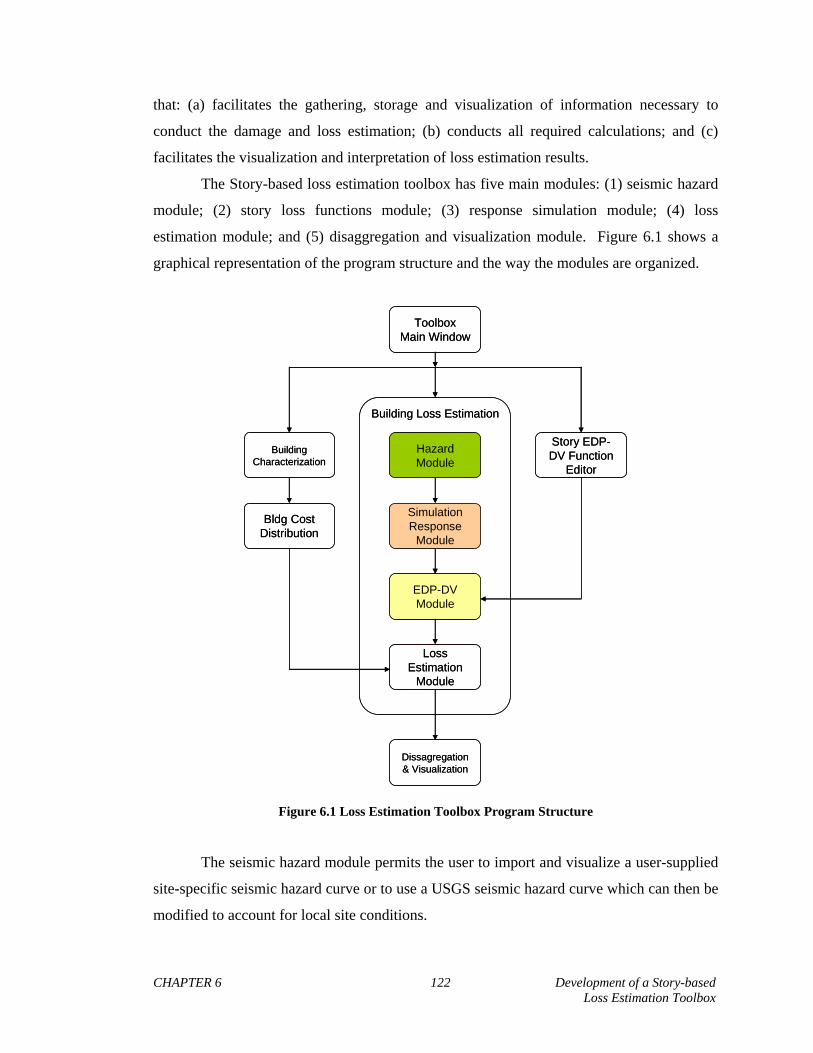
CHAPTER 6 122 Development of a Story-based Loss Estimation Toolbox
that: (a) facilitates the gathering, storage and visualization of information necessary to
conduct the damage and loss estimation; (b) conducts all required calculations; and (c)
facilitates the visualization and interpretation of loss estimation results.
The Story-based loss estimation toolbox has five main modules: (1) seismic hazard
module; (2) story loss functions module; (3) response simulation module; (4) loss
estimation module; and (5) disaggregation and visualization module. Figure 6.1 shows a
graphical representation of the program structure and the way the modules are organized.
Toolbox Main Window
Building Characterization
Story EDP-DV Function
Editor
Building Loss Estimation
Hazard Module
EDP-DV Module
SimulationResponse
Module
Loss Estimation
Module
Bldg Cost Distribution
Dissagregation& Visualization
Toolbox Main Window
Building Characterization
Story EDP-DV Function
Editor
Building Loss Estimation
Hazard Module
EDP-DV Module
SimulationResponse
Module
Loss Estimation
Module
Bldg Cost Distribution
Dissagregation& Visualization
Figure 6.1 Loss Estimation Toolbox Program Structure
The seismic hazard module permits the user to import and visualize a user-supplied
site-specific seismic hazard curve or to use a USGS seismic hazard curve which can then be
modified to account for local site conditions.

CHAPTER 6 123 Development of a Story-based Loss Estimation Toolbox
The story loss functions module calculates story loss functions that allow the
estimation of losses in individual stories as a function of scalar Engineering Demand
Parameters (EDPs) such as interstory drift ratio or peak floor acceleration. Users have the
option of using built-in (or previously computed) generic story loss functions for certain
building/use types by only knowing a small amount of information about the building such
as its structural lateral resisting system and its use. For a given building type (e.g., ductile
reinforced concrete office building) three generic loss functions are available in this module
of the toolbox: (i) structural components (assumed to be drift-sensitive); (ii) drift-sensitive
nonstructural components; and (iii) acceleration-sensitive nonstructural components. These
generic story loss functions are based on structural and nonstructural components that are
typically present in the selected building type and average distribution of construction costs
for the selected building type.
The response simulation module provides a user-friendly graphical user interface to
import and visualize response simulation results previously computed with PEER’s
OpenSees simulation platform or with other simulation software platform (e.g. SAP,
Perform, etc.). The module is capable of importing simulation results from either “cloud”
or “stripe” analyses and can import simulation results to compute the conditional
probability of collapse given (conditioned on) ground motion intensity.
The loss estimation module computes losses in the building conditioned on the
ground motion intensity and then computes several measures of seismic performance by
integrating these conditional building losses over all ground motion intensities. At the time
of this publication, the measures of seismic performance that can be computed by this
module are: (a) expected loss for a given level of ground motion intensity, and (b) expected
annual loss (EAL). Other types of results that will be implemented in the future will
include: (a) expected annual loss over a finite building life using a user-specified discount
rate; (b) net present value of the building considering earthquake losses; (c) probability of
exceeding a certain economic loss for a given ground motion intensity; (d) probability of
exceeding a certain dollar loss in the remaining life of the building; (e) economic loss
associated with a user-specified probability of exceedance.
The loss disaggregation module permits the disaggregation of economic loss to
identify the contribution of seismic events, response levels, stories, and performance groups
that primarily contribute to economic losses. Some examples of disaggregation computation
and visualization that will be included in this module include: contribution of collapse and
CHAPTER 6 124 Development of a Story-based Loss Estimation Toolbox
non-collapse building responses to economic losses, contribution of individual stories to
economic losses, disaggregation of losses due to damage in structural and nonstructural
components and identification of ground motion intensity levels primarily contributing to
expected annual losses or to specific dollar losses.
In addition to the five main modules, there are two other supplemental modules that
aid in inputting data into the toolbox. The first module, the building characterization
module, is where the user can input general building information such as the building
description, the building’s value and the building’s number of stories. This module is also
where the user will specify how the building’s value is distributed between its different
floors and substructure. The second module, the EDP-DV editor, allows the user to enter
and edit specific EDP-DV functions that relate structural response parameters directly to
economic loss (for more on EDP-DV Functions, see Chapter 3). Although toolbox has
several built-in functions, the user can to edit them, or input new functions as data and new
fragility functions become available.
6.2 GRAPHICAL USER INTER FACE
6.2.1 Building Information & Characterization
Purpose: To input general building information such as number of stories, total building
value, and building use and to define the way the total cost of the building is distributed in
each floor and substructure.
The use of this module is illustrated in Figure 6.2 in 5 steps:
Step 1: Enter in a general description of the building (e.g. name, address, owner, ..etc.). to
help identify the project for future reference.
Step2: Enter the number of stories of the building. This value is referenced multiple times
throughout the program for difference calculations.
Step3: Select the building use and type.
Step 4: Enter the total value of building. This is value can be estimated by standard cost
estimating procedures. This value is distributed to each story to calculate loss on a story-
by-story basis. Loss results are typically normalized by this value.

CHAPTER 6 125 Development of a Story-based Loss Estimation Toolbox
Step 5: Choose how the total value of the building will be distributed among the different
floors and substructure. There are four methods of distributing the value, which the user
can choose from depending on preference and how much cost information is available. The
user can specify: (a) the user can use a default distribution that was derived from typical
trends in R.S. Means cost data (Balboni, 2007), (b) the value of the foundation and use a
uniform distribution on all the stories (the value is equally distributed), (c) the value of the
foundation, the first floor, and the top floor, and the remaining value is uniformly
distributed among the remaining floors, or (d) the values for the foundation and all floors.
(1) Enter building description for reference
(2) Enter number of stories for building
(3) Select building use / type
(4) Enter value of building (replacement cost)
(5) Select method of distributing cost along height of building
Figure 6.2 Building characterization module
6.2.2 EDP-DV Function Editor
Purpose: To define, visualize, edit and delete EDP-DV functions used to by toolbox to
estimate loss.
The use of this module is illustrated in Figure 6.3.
The initial window has four option buttons to perform the following actions: (a) adding new
user-defined EDP-DV functions into the toolbox, (b) viewing existing EDP-DV functions

CHAPTER 6 126 Development of a Story-based Loss Estimation Toolbox
already entered into the toolbox (both function already built-in and user-defined), (c)
editing existing EDP-DV functions, and (d) deleting existing EDP-DV functions.
(1) Choose this button to add new EDP-DV functions
(2) Choose this button to view EDP-DV functions already inputted in the toolbox
(3) Choose this button to edit EDP-DV functions already inputted in the toolbox
(3) Choose this button to delete EDP-DV functions already inputted in the toolbox
(1) Choose this button to add new EDP-DV functions
(2) Choose this button to view EDP-DV functions already inputted in the toolbox
(3) Choose this button to edit EDP-DV functions already inputted in the toolbox
(3) Choose this button to delete EDP-DV functions already inputted in the toolbox
Figure 6.3 EDP-DV function editor module
Adding new EDP-DV functions is illustrated in Figure 6.4 in 5 steps:
Step 1: Select the type of EDP used to define the EDP-DV function. The toolbox only
considers two types of EDPs: peak interstory drifts (IDR) and peak floor accelerations
(PFA), for drift-sensitive and acceleration sensitive components respectively.
Step 2: Name the new EDP-DV function for future reference.
Step 3: Enter values of EDP-DV function using the spreadsheet-like interface. Values can
be copied and pasted in from other MS-Excel spreadsheets.
Step 4: Plot function to visualize the results and check for errors in data entry.
Step 5: Press “Add Function” button to finalize process of inputting the new function.

CHAPTER 6 127 Development of a Story-based Loss Estimation Toolbox
(1) Choose what type of EDP the function is dependent on
(2) Name the EDP-DV function for future reference
(3) Enter values of EDP-DV Function
(4) Press to plot function and check for errors
(5) Press to finalize and add function
Cancels adding EDP-DV function
(1) Choose what type of EDP the function is dependent on
(2) Name the EDP-DV function for future reference
(3) Enter values of EDP-DV Function
(4) Press to plot function and check for errors
(5) Press to finalize and add function
Cancels adding EDP-DV function
Figure 6.4 Adding EDP-DV functions
The process and interface for viewing, editing and deleting is similar and is illustrated in
Figure 6.5 in 3 steps:
Step 1: Select the EDP-DV function you want to view / edit / delete.
Step 2: Edit values as necessary (this step is not necessary if you are only viewing or
deleting functions).
Step 3: Press “Return / Accept Changes / Delete” button when finished.

CHAPTER 6 128 Development of a Story-based Loss Estimation Toolbox
(1) Choose EDP-DV function you want to view/edit/delete
(2) Edit values as if needed
(3) Press to finish viewing / editing / deleting
Press to plot function
Press to cancel
Press to close plot
(1) Choose EDP-DV function you want to view/edit/delete
(2) Edit values as if needed
(3) Press to finish viewing / editing / deleting
Press to plot function
Press to cancel
Press to close plot
Figure 6.5 Viewing / Editing / Deleting EDP-DV functions
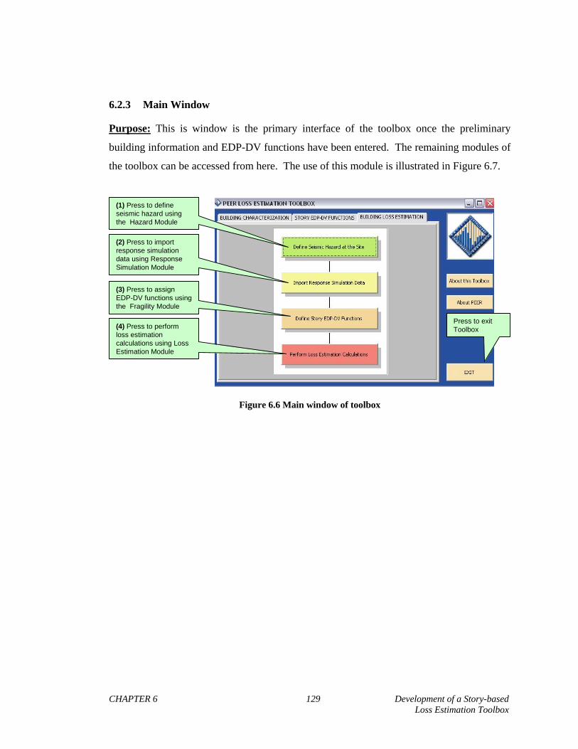
CHAPTER 6 129 Development of a Story-based Loss Estimation Toolbox
6.2.3 Main Window
Purpose: This is window is the primary interface of the toolbox once the preliminary
building information and EDP-DV functions have been entered. The remaining modules of
the toolbox can be accessed from here. The use of this module is illustrated in Figure 6.7.
(1) Press to define seismic hazard using the Hazard Module
(3) Press to assign EDP-DV functions using the Fragility Module
(2) Press to import response simulation data using Response Simulation Module
(4) Press to perform loss estimation calculations using Loss Estimation Module
Press to exit Toolbox
Figure 6.6 Main window of toolbox
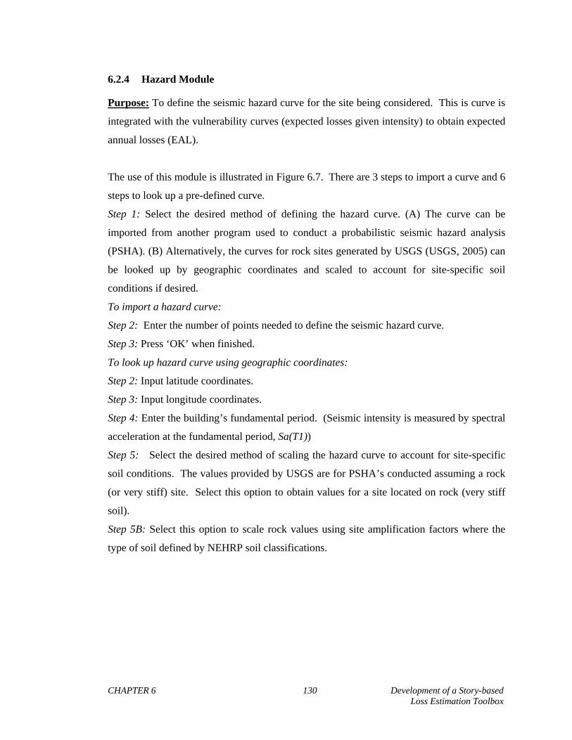
CHAPTER 6 130 Development of a Story-based Loss Estimation Toolbox
6.2.4 Hazard Module
Purpose: To define the seismic hazard curve for the site being considered. This is curve is
integrated with the vulnerability curves (expected losses given intensity) to obtain expected
annual losses (EAL).
The use of this module is illustrated in Figure 6.7. There are 3 steps to import a curve and 6
steps to look up a pre-defined curve.
Step 1: Select the desired method of defining the hazard curve. (A) The curve can be
imported from another program used to conduct a probabilistic seismic hazard analysis
(PSHA). (B) Alternatively, the curves for rock sites generated by USGS (USGS, 2005) can
be looked up by geographic coordinates and scaled to account for site-specific soil
conditions if desired.
To import a hazard curve:
Step 2: Enter the number of points needed to define the seismic hazard curve.
Step 3: Press ‘OK’ when finished.
To look up hazard curve using geographic coordinates:
Step 2: Input latitude coordinates.
Step 3: Input longitude coordinates.
Step 4: Enter the building’s fundamental period. (Seismic intensity is measured by spectral
acceleration at the fundamental period, Sa(T1))
Step 5: Select the desired method of scaling the hazard curve to account for site-specific
soil conditions. The values provided by USGS are for PSHA’s conducted assuming a rock
(or very stiff) site. Select this option to obtain values for a site located on rock (very stiff
soil).
Step 5B: Select this option to scale rock values using site amplification factors where the
type of soil defined by NEHRP soil classifications.
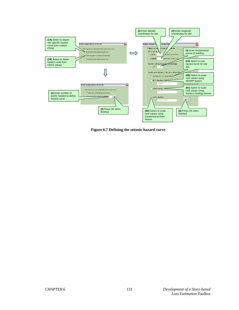
CHAPTER 6 131 Development of a Story-based Loss Estimation Toolbox
(1A) Select to import site-specific hazard curve from custom PSHA
(1B) Select to obtain hazard curve from USGS values
(2) Enter latitude coordinates for site
(3) Enter longitude coordinates for site
(4) Enter fundamental period of building
(5A) Select to use hazard curve for site ass
(5B) Select to scale rock values using NEHRP factors
(5C) Select to scale rock values using Surface Geology factors
(5D) Select to scale rock values using Geotechnical Data factors
(6) Press OK when finished
(2) Enter number of points needed to define hazard curve
(3) Press OK when finished
Figure 6.7 Defining the seismic hazard curve

CHAPTER 6 132 Development of a Story-based Loss Estimation Toolbox
6.2.5 Response simulation module
Purpose: To input response simulation data generated by incremental dynamic structural
analysis. There are two primary types of simulation data required to conduct a loss
assessment: (1) collapse data, which is used to compute the probability of collapse for the
considered building, and (2) engineering demand parameter (EDP) data, which is used to
calculate losses due to repair given the structure has not collapsed.
The use of this module is illustrated in Figure 6.8. There is 1 step to import a data from a
pre-formatted EXCEL file and 10 steps to enter the data manually.
Step 1: Select the desired method of importing the response data. (A) The module allows
data to be entered manually such that it does not matter what computer program is used to
generate the simulation data. (B) The module also is capable of importing data from an MS
EXCEL file that has been preformatted such that it can be read in by the toolbox properly.
Step 2: Enter the number ground motion records that were used in the structural analysis.
Results produced from each ground motion are used to produce statistical parameters
(median and lognormal standard deviation) for the probability of collapse and EDP (e.g.
IDR and PFA) values at each story/floor.
Step 3: Enter the number of levels of ground motion intensity that each record was scaled
to during structural analysis.
Step 4: Enter collapse data into the spreadsheet form provided. Space is provided for the
user to enter the value of seismic ground motion intensity at which the structure collapses
for each ground motion record. In addition, there are cells where the user can enter the
statistical parameters for the collapse fragility directly (median and lognormal standard
deviation of the collapse fragility function).
Step 5: Once the collapse data has been entered, press the ‘Add’ button to write the data
into the program’s memory.
Step 6: Press the ‘EDP DATA’ tab to switch to the form to enter in EDP data.
Step 7: Select the value of seismic intensity (IM level) that is currently being entered using
the pull-down menu provided.
Step 8: Enter in the EDP data generated from structural analysis. The first few lines are for
entering in peak IDRs for each story. The next few lines are for entering peak residual

CHAPTER 6 133 Development of a Story-based Loss Estimation Toolbox
interstory drifts (RIDRs). The final lines are used for entering peak ground acceleration and
PFAs.
Step 9: Once the EDP data has been entered, press the ‘Add’ button to write the data into
the programs memory.
Step 10: Press the ‘OK’ button when you are finished to save the data that has been entered
in or Press the ‘Cancel’ button to exit the window without saving the data entered.

CHAPTER 6 134 Development of a Story-based Loss Estimation Toolbox
(1A) Select to enter in simulation data manually.
(1B) Select to import simulation data from pre-formatted file
Press to visualize data once data is imported (will become active only after data has been entered).
Press RETURN to return to main menu.
(2) Enter number of ground motions considered in simulation
(3) Enter number of intensity measure (IM) levels
(7) Select IM level for EDP data currently being entered.
(8A) Enter peak IDR’s
(8B) Enter residual IDR’s
(8C) Enter PGA & PFA’s
(9) Press to add data for current IM to file once data is entered
(10A) Press to OK when finished entering all simulation data
(10B) Press to CANCEL to return to previous window without saving data entered.
(6) Press to enter EDP data
(5) Press to add data for current IM to file once data is entered(4) Enter collapse
data.
Figure 6.8 Importing response simulation data.
The following windows allow users to make adjustments to the response simulation
data after the raw values have been imported. The user will have the opportunity to make
adjustments to the parameters of the collapse fragility. Based on the final collapse fragility
parameters, the toolbox will determine if there is enough EDP data to calculate losses at
enough ground motion intensity levels to complete the integration for EAL. If there is not
enough data, the program gives users the option of extrapolating the EDP data for higher

CHAPTER 6 135 Development of a Story-based Loss Estimation Toolbox
ground motion intensity levels, or aborting the analysis. This process is illustrated in Figure
6.9 and is completed in the following 3 steps.
Step 11: After importing the raw data from response simulation, a window with a plot of the
collapse fragility will appear. Make any necessary adjustments to the collapse fragility
parameters using the textboxes provided. Users may need to modify the parameters of the
collapse fragility to account for phenomenon that influence the probability of collapse. For
instance, previous studies (Haselton and Deierlein 2007, Liel and Deierlein 2008) have
shown that spectral shape can significantly affect the collapse median, while considering
modeling uncertainty may influence the value of the lognormal standard deviation.
Step 12: Press the ‘OK’ button when the parameters of the collapse fragility have been
entered.
Step 13: Once the collapse fragility parameters have been established, the program will
check to see if there is sufficient amount of EDP data to complete the computation of EAL.
Select from the following options on how the EDP data will be extrapolated: (A)
extrapolate the EDP data for large values of ground motion intensity without smoothing,
(B) extrapolate the EDP data for large values of ground motion intensity with smoothing
using a polynomial regression, and (C) aborting the analysis and running more structural
response simulations.
The calculation of EAL involves integrating the expected losses as a function of
ground motion intensity with the seismic hazard curve (Aslani and Miranda, 2005) over the
full range of ground motion intensities up to that when the structure collapses. It was
decided that integrating up to intensity values associated with a 98% probability of collapse
would be sufficient to calculate EAL accurately. Ground motion intensities greater than
these values typically have a very low frequency of occurring and the economic loss
calculated at these intensities do not contribute a significant amount more to the total value
of EAL.
Calculation of the EAL requires expected losses for a given seismic intensity have
to be computed up to large intensities of ground motion associated with a 98% probability
of collapse. Since losses due to non-collapse are a function of peak EDP values, EDP data
for these large ground motion intensities have to be provided. This can be come difficult
when modeling collapse because many simulations at high levels of ground motion
intensity do not converge. Therefore, if not enough EDP data is provided then the user has
the option of running an extrapolation algorithm. The algorithm will extrapolate enough

CHAPTER 6 136 Development of a Story-based Loss Estimation Toolbox
EDP statistical parameters to compute enough expected losses at large intensity levels to
complete the integration.
The program also provides the user with the option of smoothing out the function
that relates EDP statistical parameters to ground motion intensity. Often at higher intensity
levels, estimates of the median and lognormal standard deviation for EDPs become less
reliable because the size of the sample of converged simulations becomes smaller. The
estimates become more erratic and may lead to less accurate estimates of the loss due to
non-collapse. The program offers the user the option to fit a 5th order polynomial to
represent the value of EDP as a function of ground motion intensity after extrapolation has
been performed.
(11A) Adjustments to the collapse median can be made here.
(11A) Adjustments to the lognormal standard deviation of the collapse probability distribution can be made here.
(12) Press to OK when finished editing the collapse parameters
(13A) Press to extrapolate EDPswithout smoothing using polynomial regression.
(13B) Press to extrapolate EDPs using polynomial regression to smooth the trends of the EDP parameters with IM level.
(13C) Press to abort analysis and run more structural analyses.
Figure 6.9 Collapse fragility adjustments and EDP extrapolation options

CHAPTER 6 137 Development of a Story-based Loss Estimation Toolbox
Once the EDP data has been extrapolated, a visualization window will appear to
display the results of the response simulation data, as show in Figure 6.10. There are
several figures displaying the following information:
Graph A: This graph plots median EDP values for each floor/story as a function of ground
motion intensity.
Graph B: This graph plots the EDPs lognormal standard deviations for each floor/story as a
function of ground motion intensity.
Graph C: This graph plots median EDP values for each floor/story along the height of the
building for particular values of ground motion intensity.
Use pull-down menu to select type of EDP to view.
Use tabs to toggle between viewing EDP data and collapse data.
Graph A: This graph plots the median EDP as a function of ground motion intensity (Sa at T1, g)
Graph B: This graph plots the EDP’slognormal standard deviation as a function of ground motion intensity (Sa at T1, g)
Graph C: This graph plots the median EDP’sat each floor/story for particular ground motion intensity levels.
Press Close button to exit and return to main window.
Figure 6.10 Response simulation visualization.
6.2.6 EDP-DV Module
Purpose: To assign EDP-DV functions to drift-sensitive structural components, drift-
sensitive nonstructural components and acceleration-sensitive nonstructural components for
each floor.
The use of this module is illustrated in Figure 6.11. There are 4 steps required to complete
this process.
Step 1: Click on the pull-down menu to select the desired floor to make EDP-DV function
assignments.

CHAPTER 6 138 Development of a Story-based Loss Estimation Toolbox
Step 2: (A) Enter the number of the EDP-DV function that is to be assigned to drift-
sensitive structural components for the floor being considered. All the EDP-DV functions
are listed and enumerated in the list box above the textboxes. Use the numbering in this list
to reference the EDP-DV functions when making assignments. Repeat for the drift-
sensitive and acceleration-sensitive nonstructural components. (B) Alternatively, the
assignments can be made by typing in the number of the EDP-DV function directly into the
spreadsheet form provided.
Step 3: Press the ‘ASSIGN’ button to write the assignments into the spreadsheet form.
Step 4: Press the ‘OK’ button to save the EDP-DV assignments when finished. To return to
the Main window without saving the assignments press the ‘CANCEL’ button.
(1) Use pull-down menu to select the floor for which EDP-DV functions will be assigned.
This part of the form lists the EDP-DV functions currently stored in the toolbox. Each function is numbered to use as referenced.
(2A) Enter number of the EDP-DV function to be assigned for the drift-sensitive structural components. Repeat for nonstructural components.
(3) Press ASSIGN button to enter function assignments into spreadsheet form.
(2B) Alternatively, EDP-DV function numbers can be entered directly into the spreadsheet form.
(4A) Press OK button to save assignments and return to main window.
(4B) Press CANCEL button to return to main window without saving assignments.
Figure 6.11 Assigning EDP-DV functions.
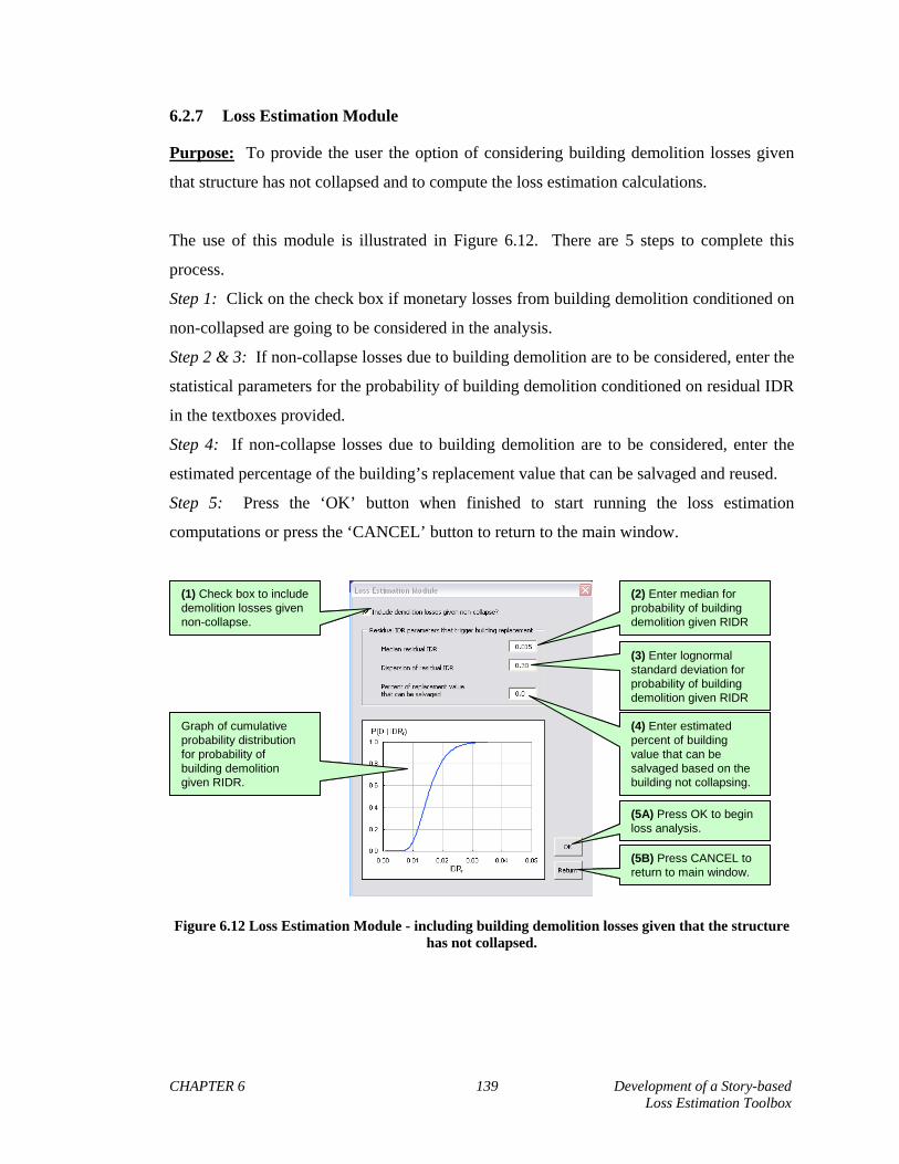
CHAPTER 6 139 Development of a Story-based Loss Estimation Toolbox
6.2.7 Loss Estimation Module
Purpose: To provide the user the option of considering building demolition losses given
that structure has not collapsed and to compute the loss estimation calculations.
The use of this module is illustrated in Figure 6.12. There are 5 steps to complete this
process.
Step 1: Click on the check box if monetary losses from building demolition conditioned on
non-collapsed are going to be considered in the analysis.
Step 2 & 3: If non-collapse losses due to building demolition are to be considered, enter the
statistical parameters for the probability of building demolition conditioned on residual IDR
in the textboxes provided.
Step 4: If non-collapse losses due to building demolition are to be considered, enter the
estimated percentage of the building’s replacement value that can be salvaged and reused.
Step 5: Press the ‘OK’ button when finished to start running the loss estimation
computations or press the ‘CANCEL’ button to return to the main window.
(1) Check box to include demolition losses given non-collapse.
(2) Enter median for probability of building demolition given RIDR
(3) Enter lognormal standard deviation for probability of building demolition given RIDR
(4) Enter estimated percent of building value that can be salvaged based on the building not collapsing.
(5A) Press OK to begin loss analysis.
(5B) Press CANCEL to return to main window.
Graph of cumulative probability distribution for probability of building demolition given RIDR.
Figure 6.12 Loss Estimation Module - including building demolition losses given that the structure has not collapsed.

CHAPTER 6 140 Development of a Story-based Loss Estimation Toolbox
6.2.8 Loss Disaggregation and Visualization Module
Purpose: To display the results from the loss estimation computations. The module
displays total losses and disaggregated losses. Results for both expected losses as a
function of ground motion intensity and EALs are provided.
The types of results for expected loss as a function of ground motion intensity are illustrated
in Figure 6.13.
Graph A: This graph plots the total expected losses as a function of increasing levels of
ground motion intensity. This type of information can be used for so called “scenario-
based” events where the monetary loss can be found for a ground motion intensity of
particular interest. For instance, this graph may be used to obtain expected monetary loss
given the ground motion intensity level associated with the design basis earthquake (DBE),
the event with an exceedance rate of occurrence of 10% in 50 years. Also plotted on this
graph are the losses disaggregated with respect to losses given that the building has
collapsed, losses given that the building has not collapsed due to building demolition, and
losses given that the building has not collapsed due to repair costs. For each level of ground
motion intensity, the user can identify how much each of these sources of economic losses
contribute to the overall losses.
Graph B: This graph plots the loss given that the building has not collapsed due to repair
costs as a function of ground motion intensity, disaggregated by floor. This information is
useful to identify which floor(s) are contributing the most to losses due to non-collapse
caused by repair costs.
Graph C: This graph plots the loss given that the building has not collapsed due to repair
costs as a function of ground motion intensity disaggregated by types of building
components grouped as follows: (1) drift-sensitive structural components (2) drift-sensitive
nonstructural components and (3) acceleration-sensitive nonstructural components.

CHAPTER 6 141 Development of a Story-based Loss Estimation Toolbox
Use tabs to toggle between results for expected loss as a function of ground motion intensity and expected annual results.
Use pull-down menu to select type of graph (line or bar) to display expected losses
Graph B: This graph plots expected loss results as a function of ground motion intensity. Also shown are the expected results for loss disaggregated for collapse losses, non-collapse losses due to demolition and non-collapse losses due to repair costs.
Graph A: This graph plots expected non-collapse losses due to repair disaggregated by floor/story.
Press RETURN button to return to main window.
Press SAVE & CLOSE button to save loss results in output file.
Graph C: This graph plots expected non-collapse losses due to repair disaggregated by component types.
Figure 6.13 Total and disaggregation results for expected economic losses as a function of ground motion intensity
The types of results for expected loss as a function of ground motion intensity are
illustrated in Figure 6.14. The total EAL and disaggregated EALs are tabulated in the upper
left part of the window.
Graph A: This pie graph plots the EAL disaggregated by collapse losses, non-collapse
losses due to building demolition and non-collapse losses due to repair costs.
Graph B: This pie graph plots the EAL of non-collapse losses due to repair costs
disaggregated by drift-sensitive structural components (ST | IDR), drift-sensitive

CHAPTER 6 142 Development of a Story-based Loss Estimation Toolbox
nonstructural components (NS | IDR) and acceleration-sensitive nonstructural components
(NS | PFA).
Graph C: This bar graph plots the total EAL disaggregated by ground motion intensity
level. Each bar represents the amount of EAL for intensities up to the value shown below
the bar.
Graph D: This bar graph plots non-collapse losses due to repair costs disaggregated by both
component type and intensity level.
Graph B: This graph plots EAL results for non-collapse losses due to repair disaggregated by component type
This part of the form summarizes key values for the EAL results
Graph C: This graph plots EAL results that have been disaggregated by ground motion intensity level.
Graph A: This graph plots EAL results disaggregated by collapse losses, non-collapse losses due to demolition and non-collapse losses due to repair. Press RETURN
button to return to main window.
Press SAVE & CLOSE button to save loss results in output file.
Graph D: This graph plots EAL of non-collapse losses due to repair disaggregated by both component type and ground motion intensity level.
Figure 6.14 Total and disaggregation results for expected annual losses.

CHAPTER 7 143 Benchmarking Seismic-induced Economic Losses Using Story-based Loss Estimation
CHAPTER 7
7 BENCHMARKING SEISMIC-INDUCED ECONOMIC LOSSES USING STORY-BASED
LOSS ESTIMATION
This chapter is based on the following publications:
Ramirez, C.M., and Miranda, E. (2009), “Story-based Building-Specific Loss Estimation,”
Journal of Structural Engineering, (in preparation).
Ramirez, C.M., A.B. Liel, J. Mitrani-Reiser, C.B. Haselton, A.D. Spear, J. Steiner, G.G.
Deierlein, E. Miranda. (2009), “Performance-Based Predictions of Earthquake-Induced
Economic Losses in Reinforced Concrete Frame Structures,” Earthquake Spectra, (in
preparation).
7.1 AUTHORSHIP OF CHAPTER
Ramirez led this research effort that consisted of two primary phases. The first phase
involved evaluating economic losses using a component-based approach using a computer
tool (MDLA) developed by Mitrani-Reiser (2007). The results of this phase will be
published in the second paper listed above. The second phase repeated the loss analyses
using the story-based loss estimation approach presented in Chapter 3 and the computer tool
developed in Chapter 6.
Liel computed and supplied the structural analysis for the non-ductile ductile
reinforced concrete moment frame buildings in this study and wrote/edited portions of this
publication. Mitrani-Reiser provided the component-based loss estimation computer tool
(MDLA) used in the first phase of this investigation and wrote/edited portions of this
publication. Spear and Steiner developed the architectural layouts and cost estimations in

CHAPTER 7 144 Benchmarking Seismic-induced Economic Losses Using Story-based Loss Estimation
this study, and was responsible for completing the economic loss analyses for the results
produced by MDLA. Haselton computed and supplied the structural analysis for the ductile
reinforced concrete moment frame building data for used in this study, helped edit the
publication and served as an advisor for this study. Miranda and Deierlein served as
advisors to this investigation.
7.2 INTRODUCTION
Recent earthquakes in California, particularly Loma Prieta (1989) and Northridge
(1994), have demonstrated that while modern U.S. building codes have been relatively
successful in protecting human life in moderate magnitude events, significant economic
losses may still occur. These losses suggest that building owners and other stakeholders
may wish to evaluate other aspects of building seismic performance beyond protecting life-
safety. The Pacific Earthquake Engineering Research (PEER) Center has established a
framework for performance-based earthquake engineering (PBEE) that can be used to
assess several metrics of seismic performance, including economic losses, downtime and
number of fatalities (Krawinkler and Miranda, 2004). By providing quantitative measures
of structural performance, PBEE can be used to consider possible earthquake economic
losses and loss mitigation strategies when making design decisions.
Methodologies for predicting economic losses in earthquakes can be characterized
as either regional loss estimation or building-specific loss estimation. Regional loss
estimation predicts earthquake economic losses in a broad geographical area, by estimating
building inventory data and categorizing buildings into generic structural types to evaluate
earthquake performance In 1992, the Federal Emergency Management Agency (FEMA)
and the National Institute of Building Sciences (NIBS) began funding the development of a
geographic information system (GIS)-based regional loss estimation methodology
(Whitman et al. 1997), which eventually was implemented in the widely-used computer
tool, HAZUS (National Institute of Building Sciences, 1997). Based on a building’s lateral
force resisting system, height and occupancy, structural response and damage is calculated
using pre-established capacity and fragility functions, to determine repair costs.
Generalizing buildings in this manner provides a simple and widely applicable way of

CHAPTER 7 145 Benchmarking Seismic-induced Economic Losses Using Story-based Loss Estimation
estimating losses, but these methods cannot capture unique aspects of a specific building’s
structural and nonstructural design and are not reliable for individual structures.
Building-specific earthquake-induced economic losses can be computed by
evaluating damage in structural and non-structural components on the basis of structural
analysis of an individual building to estimate damage and determining the cost of repairing
this damage. Damage states are defined for each component in the building based on the
different repair actions needed to restore the components to its original state. Scholl (1979)
initially introduced a building-specific loss estimation methodology, which was further
developed by a variety of researchers over the past 20 years (Kustu et al. 1982; Gunturi and
Shah 1993; Singhal and Kiremidjian 1996). Porter and Kiremidjian 2001 established an
assembly-based approach to probabilistic performance evaluation that considers building
assemblies (groups of building components) at a greater level of detail than previous
techniques. Extending this work, PEER’s loss estimation methodology incorporates items
such as probabilistic seismic hazard analysis and the probability of structural collapse,
establishing a comprehensive framework for performance assessment. PEER’s framework
was documented by Miranda et al, (2004), Aslani and Miranda (2005) and Mitrani-Reiser
(2007). Mitrani-Reiser (2007) also implemented the framework into a computational tool,
the MATLAB Damage and Loss Analysis (MDLA) toolbox, which calculates seismic
economic losses for reinforced concrete (RC) frame structures. A simplified approach to
PEER’s loss methodology, referred to as story-based loss estimation, was developed and
documented in Chapter 3 of this dissertation and also implemented into a computer tool.
Mitrani-Reiser used the MLDA toolbox to benchmark the performance of different
design variations of a modern four-story RC office building for a site in Los Angeles,
California (Goulet et al. 2007). Their investigation studied the effects of different design
alternatives on predictions of collapse and direct economic losses, but because its scope was
limited to one type of building, other structural parameters – such as the building height,
bay width, and foundation design assumptions – were not examined. Haselton and
Deierlein (2007) took a broader approach in a separate investigation that analyzed a set of
archetypical RC frame buildings, to examine how structural design variations (height, bay
width, etc.) and other key code provisions (strong-column weak-beam requirements,
maximum interstory drift ratio, and R-factor) influenced performance; however, this
research focused on collapse performance, and did not consider economic losses.

CHAPTER 7 146 Benchmarking Seismic-induced Economic Losses Using Story-based Loss Estimation
In this study, the same set of archetypical modern RC buildings (Haselton 2007) is
investigated to benchmark the magnitude of the economic losses possible in modern code-
conforming RC frame structures in high seismic areas and to quantify the effect of
important design variables on estimated losses, using PEER’s story-based loss estimation
method (developed in Chapter 3), and the associated computer toolbox that implements this
approach (described in Chapter 6). Structural design parameters considered include
building height, type of framing system, strength and stiffness variability along the building
height, foundation design assumptions. We also investigate how selected code provisions,
primarily the design R-factor and the strong column-weak beam ratio, affect seismic
performance in terms of economic losses. Additionally, architectural variations are also
examined to see if they have a significant effect on predicted economic losses. This
investigation focuses on modern code-conforming, moment-resisting frame buildings
(ductile reinforced concrete), primarily used as office space; however, a brief comparison to
non-ductile reinforced concrete frame buildings will be conducted to evaluate the difference
in risk associated with older buildings. In this study, seismic performance is solely based
on economic losses (defined here as the cost of repairing or replacing structural and
nonstructural components damaged by earthquakes) and seismic performance metrics such
as downtime and fatalities are not considered.
7.3 LOSS ESTIMATION PROCEDURE
The decision variables considered in this study are all associated with the
repair/replacement effort needed to return a building back to its original (undamaged) state
after an earthquake and the repair/replacement effort is quantified in dollar terms. The
mean total repair cost for each hazard level, also known as the vulnerability function, is
calculated for the study RC frame buildings by summing the mean repair cost for all
damageable components in the building. The repair cost is disaggregated at each hazard
level to illustrate the contribution of each damageable building component type to the total
loss (Miranda et al. 2004, Aslani and Miranda 2005). Finally, the expected annual loss is
computed to estimate the amount an owner could expect to pay on average yearly to repair
earthquake damage, considering the frequency of occurrence and severity of all possible
earthquakes at the site.

CHAPTER 7 147 Benchmarking Seismic-induced Economic Losses Using Story-based Loss Estimation
The damage and loss analyses portions of the PEER methodology are evaluated in
this study using the computer toolbox described in Chapter 6 of this dissertation. In order to
estimate economic losses in a structure, the toolbox only needs the estimated replacement
value of the building and input from the hazard and structural analysis results. The loss is
calculated using story EDP-DV functions built into the toolbox, which relate response
demand parameters to expected loss directly. Interested readers are directed to Chapter 3 of
this dissertation for a more detailed explanation of the equations used in this study.
7.4 DESCRIPTION OF BUILDINGS
In this study, the performance-based loss estimation framework is applied to
evaluate earthquake-induced economic losses in modern, code-conforming RC frame
structures. All buildings in this study are assumed to be located at a site in the Los Angeles
basin, south of downtown Los Angeles. The location was selected as a typical urban
California site with high levels of seismicity in the transition zone of IBC design maps, but
not subject to near-fault directivity effects (Haselton et al. 2007). The site-specific hazard
curve (Figure 7.1), which predicts the likelihood of experiencing a ground motion
exceeding a specified intensity at the site of interest, is obtained from probabilistic seismic
hazard analysis by Goulet et al. (2007). Ground motion intensity in this study is quantified
using spectral acceleration at fundamental period, Sa(T1) (note that in the figures and tables
in this chapter will denote this value as Sa for brevity, however, it is implied that this value
is at the fundamental period).

CHAPTER 7 148 Benchmarking Seismic-induced Economic Losses Using Story-based Loss Estimation
1.0E-05
1.0E-04
1.0E-03
1.0E-02
1.0E-01
1.0E+00
1.0E+01
0.01 0.1 1 10IM = Sa(T1)
(IM)
T1 = 1 sec
T1 = 2 sec
1.0E-05
1.0E-04
1.0E-03
1.0E-02
1.0E-01
1.0E+00
1.0E+01
0.01 0.1 1 10IM = Sa(T1)
(IM)
T1 = 1 sec
T1 = 2 sec
Figure 7.1 Ground motion probabilistic seismic hazard curves (Goulet et al., 200&)
The reinforced concrete frame structures were designed according to the 2003
International Building Code and related ACI and ASCE provisions by Haselton and
Deierlein (2007) (ACI 2002; ASCE 2002; ICC 2003,). Seismic design is based on the
mapped seismicity at the site of interest with Ss = 1.5g and S1 = 0.6g (these values define
corners of the design spectra, which is associated with a mean annual frequency of
approximately 10% in 50 years as specified in the International Building Code (ICC 2003)).
Each of the structures are designed to fully comply with the building code provisions for
special moment frames, including strong column-weak beam ratios, joint shear strength and
detailing provisions, and requirements for strength and stiffness. The buildings range in
height from 1 to 20 stories, and include both perimeter and space frame systems. Table 7.1
details the design parameters of the 30 buildings evaluated in this study. The shorter
buildings (1, 2 and 4-stories) have a plan area of 120 ft. x 180 ft. The taller buildings (8,
12, and 20 stories) have a smaller footprint, reflecting typical ratios of usable floor area to
lot sizes in high rise construction.
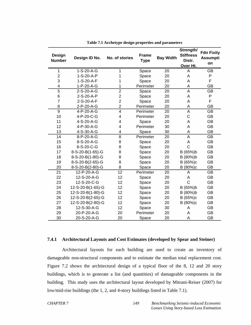
CHAPTER 7 149 Benchmarking Seismic-induced Economic Losses Using Story-based Loss Estimation
Table 7.1 Archetype design properties and parameters
Design Number
Design ID No. No. of storiesFrame Type
Bay Width
Strength/Stiffness
Distr. Over Ht.
Fdn Fixity Assumpti
on
1 1-S-20-A-G 1 Space 20 A GB2 1-S-20-A-P 1 Space 20 A P3 1-S-20-A-F 1 Space 20 A F4 1-P-20-A-G 1 Perimeter 20 A GB5 2-S-20-A-G 2 Space 20 A GB6 2-S-20-A-P 2 Space 20 A P7 2-S-20-A-F 2 Space 20 A F8 2-P-20-A-G 2 Perimeter 20 A GB9 4-P-20-A-G 4 Perimeter 20 A GB10 4-P-20-C-G 4 Perimeter 20 C GB11 4-S-20-A-G 4 Space 20 A GB12 4-P-30-A-G 4 Perimeter 30 A GB13 4-S-30-A-G 4 Space 30 A GB14 8-P-20-A-G 8 Perimeter 20 A GB15 8-S-20-A-G 8 Space 20 A GB16 8-S-20-C-G 8 Space 20 C GB17 8-S-20-B(1-65)-G 8 Space 20 B (65%)b GB18 8-S-20-B(1-80)-G 8 Space 20 B (80%)b GB19 8-S-20-B(2-65)-G 8 Space 20 B (65%)c GB20 8-S-20-B(2-80)-G 8 Space 20 B (80%)c GB21 12-P-20-A-G 12 Perimeter 20 A GB22 12-S-20-A-G 12 Space 20 A GB23 12-S-20-C-G 12 Space 20 C GB24 12-S-20-B(1-65)-G 12 Space 20 B (65%)b GB25 12-S-20-B(1-80)-G 12 Space 20 B (80%)b GB26 12-S-20-B(2-65)-G 12 Space 20 B (65%)c GB27 12-S-20-B(2-80)-G 12 Space 20 B (80%)c GB28 12-S-30-A-G 12 Space 30 A GB29 20-P-20-A-G 20 Perimeter 20 A GB30 20-S-20-A-G 20 Space 20 A GB
7.4.1 Architectural Layouts and Cost Estimates (developed by Spear and Steiner)
Architectural layouts for each building are used to create an inventory of
damageable non-structural components and to estimate the median total replacement cost.
Figure 7.2 shows the architectural design of a typical floor of the 8, 12 and 20 story
buildings, which is to generate a list (and quantities) of damageable components in the
building. This study uses the architectural layout developed by Mitrani-Reiser (2007) for
low/mid-rise buildings (the 1, 2, and 4-story buildings listed in Table 7.1).

CHAPTER 7 150 Benchmarking Seismic-induced Economic Losses Using Story-based Loss Estimation
This study also examined the effect of variations in two primary architectural design
parameters on the seismic loss estimations: the amount of partitions, and the quality of
interior and exterior finishes. Previous studies have shown that non-structural components
represent a substantial portion of the investment in office buildings (Taghavi and Miranda,
2002) and often also account for most of the economical losses (Miranda et al 2004, Aslani
and Miranda 2005). Damaged partitions, in particular, have been identified as a large
contributor to economic losses (Mitrani-Reiser 2007). The quantity of partitions is directly
related to the percent of open office space dictated by the architectural layout. Here, open
office space is defined as space that is occupied by multiple occupants and, in many cases,
segmented by removable, partial height partitions – a group of cubicles, for example,
represents open office space, unlike a single-occupant office, which is enclosed by non-
removable partitions. The original architectural layout (Figure 7.2) has 36% open office
space. Two alternate high-rise layouts with different percentages of open office space (14%
and 58%) to investigate how the quantity of partitions affected loss results. We also
investigated how finish quality affects losses estimations, by evaluating a building with
higher level of finishes, characteristic of a high-end tenant.
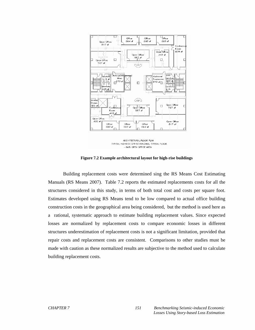
CHAPTER 7 151 Benchmarking Seismic-induced Economic Losses Using Story-based Loss Estimation
Figure 7.2 Example architectural layout for high-rise buildings
Building replacement costs were determined sing the RS Means Cost Estimating
Manuals (RS Means 2007). Table 7.2 reports the estimated replacements costs for all the
structures considered in this study, in terms of both total cost and costs per square foot.
Estimates developed using RS Means tend to be low compared to actual office building
construction costs in the geographical area being considered, but the method is used here as
a rational, systematic approach to estimate building replacement values. Since expected
losses are normalized by replacement costs to compare economic losses in different
structures underestimation of replacement costs is not a significant limitation, provided that
repair costs and replacement costs are consistent. Comparisons to other studies must be
made with caution as these normalized results are subjective to the method used to calculate
building replacement costs.

CHAPTER 7 152 Benchmarking Seismic-induced Economic Losses Using Story-based Loss Estimation
Table 7.2 Cost estimates for structures studied
Total Cost Cost per s.f. Total Cost Cost per s.f.
1-story 21,600 $3,310,000 $153 $3,180,000 $147
2-story 43,200 $6,070,000 $140 $6,510,000 $151
4-story 86,400 $12,500,000 $144 $12,000,000 $138
8-story 115,200 $19,900,000 $173 $19,400,000 $168
12-story 172,800 $29,100,000 $168 $28,100,000 $163
20-story 288,000 $49,500,000 $172 $47,900,000 $166
Space Frame Perimeter Frame
120'x180'
Number of Stories
Footprint
120'x120'
Floor Area (sf)
7.4.2 Nonlinear Simulation Models and Structural Analysis (computed by Liel and Haselton)
Each of the RC frame structures of interest in this study was modeled in OpenSees
(PEER 2006), using a two-dimensional, three-bay model of the lateral resisting system and
a leaning (P-Δ) column. The model does not incorporate strength or stiffness from
components designed to resist gravity loads only. Beams and columns are modeled with
concentrated plastic hinge (lumped plasticity) elements, which employs a material model
developed by Ibarra et al.(2005). This model is defined by a monotonic backbone and
associated hysteretic rules, such that it can capture critical aspects of strength and stiffness
deterioration for predicting structural behavior up to collapse. Model parameters for RC
elements are predicted from design and detailing parameters on the basis of empirical
relationships developed from calibrating the material model to experimental data from more
than 250 tests of RC columns (Haselton et al. 2007). All model parameters represent
expected (average) values. Haselton and Deierlein (2007) have shown that the lumped
plasticity modeling approach provides reasonable results, compared to fiber-element
models, at low levels of deformation and, in addition, captures material nonlinearities as the
structure approaches collapse.
Nonlinear simulation models for RC frames are analyzed using the incremental
dynamic analysis (IDA) technique (Vamvatsikos and Cornell, 2002). The analysis utilizes
a suite of ground motion records, in order to capture the effects of variation in ground

CHAPTER 7 153 Benchmarking Seismic-induced Economic Losses Using Story-based Loss Estimation
motion characteristics, such as frequency content, on the response. Selected ground
motions records are from large magnitude events, recorded at moderate fault-rupture
distances on stiff soil or rock sites (ATC, 2008). In IDA, the model is subjected to each
ground motion, recording the dynamic response (EDPs). The ground motion record is
subsequently scaled to increasing levels of intensity until collapse occurs from lateral
dynamic instability. This process is repeated for all ground motions in the set.
The outcome of IDA is the statistical prediction of critical engineering demand
parameters (EDP) at a number of ground motion intensities (stripes), and a collapse fragility
function, which describes the probability of collapse as a function of the ground motion
intensity. At lower ground motion intensities, losses are dominated by non-collapse results,
particularly damage to drift and acceleration-sensitive nonstructural components and
contents. Examples of EDPs used to calculate non-collapse losses are shown in Figure 7.3
for a 4-story space frame (4-S-20-A-G). Damage in individual components and associated
repair costs are computed from distributions in EDPs obtained at each intensity level.
1
2
3
4
0 0.02 0.04 0.06
PEAK IDR
0.05
0.25
0.50
1.00
2.00
STORY
Sa Values
2
3
4
5
0 1 2
PEAK FLR ACCEL [g]
FLOOR
1
2
3
4
0 0.02 0.04 0.06
PEAK IDR
0.05
0.25
0.50
1.00
2.00
STORY
Sa Values
2
3
4
5
0 1 2
PEAK FLR ACCEL [g]
FLOOR
Figure 7.3 Peak EDPs along building height for Design 4-S-20-A-G (Hazelton and Deierlein, 2007)
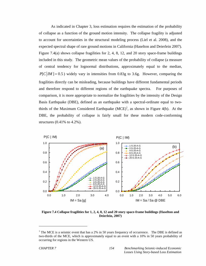
CHAPTER 7 154 Benchmarking Seismic-induced Economic Losses Using Story-based Loss Estimation
As indicated in Chapter 3, loss estimation requires the estimation of the probability
of collapse as a function of the ground motion intensity. The collapse fragility is adjusted
to account for uncertainties in the structural modeling process (Liel et al. 2008), and the
expected spectral shape of rare ground motions in California (Haselton and Deierlein 2007).
Figure 7.4(a) shows collapse fragilities for 2, 4, 8, 12, and 20 story space-frame buildings
included in this study. The geometric mean values of the probability of collapse (a measure
of central tendency for lognormal distributions, approximately equal to the median,
[ ] 0.5P C IM ) widely vary in intensities from 0.83g to 3.6g. However, comparing the
fragilities directly can be misleading, because buildings have different fundamental periods
and therefore respond to different regions of the earthquake spectra. For purposes of
comparison, it is more appropriate to normalize the fragilities by the intensity of the Design
Basis Earthquake (DBE), defined as an earthquake with a spectral-ordinate equal to two-
thirds of the Maximum Considered Earthquake (MCE)1, as shown in Figure 4(b). At the
DBE, the probability of collapse is fairly small for these modern code-conforming
structures (0.41% to 4.2%).
0.0
0.2
0.4
0.6
0.8
1.0
0.0 1.0 2.0 3.0 4.0
IM = Sa [g]
1-S-20-A-G2-S-20-A-G4-S-20-A-G8-S-20-A-G12-S-20-A-G20-S-20-A-G
P(C | IM)
(a)
0.0
0.2
0.4
0.6
0.8
1.0
0.0 1.0 2.0 3.0 4.0
IM = Sa [g]
1-S-20-A-G2-S-20-A-G4-S-20-A-G8-S-20-A-G12-S-20-A-G20-S-20-A-G
P(C | IM)
(a)
0.0
0.2
0.4
0.6
0.8
1.0
0.0 1.0 2.0 3.0 4.0 5.0 6.0
IM = Sa / Sa @ DBE
1-S-20-A-G2-S-20-A-G4-S-20-A-G8-S-20-A-G12-S-20-A-G20-S-20-A-G
P(C | IM)
(b)
0.0
0.2
0.4
0.6
0.8
1.0
0.0 1.0 2.0 3.0 4.0 5.0 6.0
IM = Sa / Sa @ DBE
1-S-20-A-G2-S-20-A-G4-S-20-A-G8-S-20-A-G12-S-20-A-G20-S-20-A-G
P(C | IM)
(b)
Figure 7.4 Collapse fragilities for 1, 2, 4, 8, 12 and 20 story space-frame buildings (Haselton and Deierlein, 2007)
1 The MCE is a seismic event that has a 2% in 50 years frequency of occurrence. The DBE is defined as two-thirds of the MCE, which is approximately equal to an event with a 10% in 50 years probability of occurring for regions in the Western US.
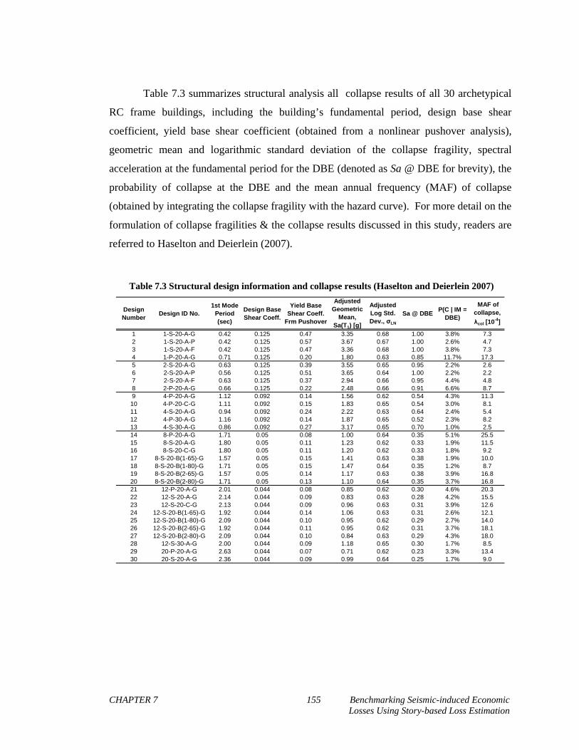
CHAPTER 7 155 Benchmarking Seismic-induced Economic Losses Using Story-based Loss Estimation
Table 7.3 summarizes structural analysis all collapse results of all 30 archetypical
RC frame buildings, including the building’s fundamental period, design base shear
coefficient, yield base shear coefficient (obtained from a nonlinear pushover analysis),
geometric mean and logarithmic standard deviation of the collapse fragility, spectral
acceleration at the fundamental period for the DBE (denoted as Sa @ DBE for brevity), the
probability of collapse at the DBE and the mean annual frequency (MAF) of collapse
(obtained by integrating the collapse fragility with the hazard curve). For more detail on the
formulation of collapse fragilities & the collapse results discussed in this study, readers are
referred to Haselton and Deierlein (2007).
Table 7.3 Structural design information and collapse results (Haselton and Deierlein 2007)
Design Number
Design ID No.1st Mode
Period (sec)
Design Base Shear Coeff.
Yield Base Shear Coeff.
Frm Pushover
Adjusted Geometric
Mean, Sa(T1) [g]
Adjusted Log Std. Dev., σLN
Sa @ DBEP(C | IM =
DBE)
MAF of collapse,
λcol [10-4]
1 1-S-20-A-G 0.42 0.125 0.47 3.35 0.68 1.00 3.8% 7.32 1-S-20-A-P 0.42 0.125 0.57 3.67 0.67 1.00 2.6% 4.73 1-S-20-A-F 0.42 0.125 0.47 3.36 0.68 1.00 3.8% 7.34 1-P-20-A-G 0.71 0.125 0.20 1.80 0.63 0.85 11.7% 17.35 2-S-20-A-G 0.63 0.125 0.39 3.55 0.65 0.95 2.2% 2.66 2-S-20-A-P 0.56 0.125 0.51 3.65 0.64 1.00 2.2% 2.27 2-S-20-A-F 0.63 0.125 0.37 2.94 0.66 0.95 4.4% 4.88 2-P-20-A-G 0.66 0.125 0.22 2.48 0.66 0.91 6.6% 8.79 4-P-20-A-G 1.12 0.092 0.14 1.56 0.62 0.54 4.3% 11.310 4-P-20-C-G 1.11 0.092 0.15 1.83 0.65 0.54 3.0% 8.111 4-S-20-A-G 0.94 0.092 0.24 2.22 0.63 0.64 2.4% 5.412 4-P-30-A-G 1.16 0.092 0.14 1.87 0.65 0.52 2.3% 8.213 4-S-30-A-G 0.86 0.092 0.27 3.17 0.65 0.70 1.0% 2.514 8-P-20-A-G 1.71 0.05 0.08 1.00 0.64 0.35 5.1% 25.515 8-S-20-A-G 1.80 0.05 0.11 1.23 0.62 0.33 1.9% 11.516 8-S-20-C-G 1.80 0.05 0.11 1.20 0.62 0.33 1.8% 9.217 8-S-20-B(1-65)-G 1.57 0.05 0.15 1.41 0.63 0.38 1.9% 10.018 8-S-20-B(1-80)-G 1.71 0.05 0.15 1.47 0.64 0.35 1.2% 8.719 8-S-20-B(2-65)-G 1.57 0.05 0.14 1.17 0.63 0.38 3.9% 16.820 8-S-20-B(2-80)-G 1.71 0.05 0.13 1.10 0.64 0.35 3.7% 16.821 12-P-20-A-G 2.01 0.044 0.08 0.85 0.62 0.30 4.6% 20.322 12-S-20-A-G 2.14 0.044 0.09 0.83 0.63 0.28 4.2% 15.523 12-S-20-C-G 2.13 0.044 0.09 0.96 0.63 0.31 3.9% 12.624 12-S-20-B(1-65)-G 1.92 0.044 0.14 1.06 0.63 0.31 2.6% 12.125 12-S-20-B(1-80)-G 2.09 0.044 0.10 0.95 0.62 0.29 2.7% 14.026 12-S-20-B(2-65)-G 1.92 0.044 0.11 0.95 0.62 0.31 3.7% 18.127 12-S-20-B(2-80)-G 2.09 0.044 0.10 0.84 0.63 0.29 4.3% 18.028 12-S-30-A-G 2.00 0.044 0.09 1.18 0.65 0.30 1.7% 8.529 20-P-20-A-G 2.63 0.044 0.07 0.71 0.62 0.23 3.3% 13.430 20-S-20-A-G 2.36 0.044 0.09 0.99 0.64 0.25 1.7% 9.0

CHAPTER 7 156 Benchmarking Seismic-induced Economic Losses Using Story-based Loss Estimation
7.5 ECONOMIC LOSSES
Economic losses were estimated for all 30 buildings in Table 1 in order to evaluate
seismic performance of modern RC frame buildings and to quantify the effects of important
design variables on economic losses. Metrics of economic loss of interest include the
expected value of the loss at the DBE, expected annual losses (EAL), and the present value
(PV) of life-cycle losses. The results of loss estimation are summarized in Table 7.4.
Table 7.4 Expected losses and intensity levels
Design Number
Design ID No. Sa @ DBELoss at DBE [%]
Normalized EAL [%]
1 1-S-20-A-G 1.00 32.3% 1.10%2 1-S-20-A-P 1.00 30.4% 1.10%3 1-S-20-A-F 1.00 32.4% 1.11%4 1-P-20-A-G 0.85 54.2% 3.31%5 2-S-20-A-G 0.95 30.9% 1.15%6 2-S-20-A-P 1.00 27.9% 0.97%7 2-S-20-A-F 0.95 31.9% 1.14%8 2-P-20-A-G 0.91 35.0% 1.22%9 4-P-20-A-G 0.54 30.7% 1.33%
10 4-P-20-C-G 0.54 29.2% 1.30%11 4-S-20-A-G 0.64 25.8% 1.03%12 4-P-30-A-G 0.52 31.4% 1.42%13 4-S-30-A-G 0.70 24.2% 0.91%14 8-P-20-A-G 0.35 25.1% 0.95%15 8-S-20-A-G 0.33 23.9% 1.11%16 8-S-20-C-G 0.33 24.3% 1.11%17 8-S-20-B(1-65)-G 0.38 19.7% 0.89%18 8-S-20-B(1-80)-G 0.35 21.8% 1.05%19 8-S-20-B(2-65)-G 0.38 20.1% 0.89%20 8-S-20-B(2-80)-G 0.35 22.1% 1.04%21 12-P-20-A-G 0.30 20.8% 0.65%22 12-S-20-A-G 0.28 20.7% 0.69%23 12-S-20-C-G 0.31 22.2% 0.87%24 12-S-20-B(1-65)-G 0.31 18.0% 0.68%25 12-S-20-B(1-80)-G 0.29 18.9% 0.67%26 12-S-20-B(2-65)-G 0.31 18.4% 0.68%27 12-S-20-B(2-80)-G 0.29 19.9% 0.69%28 12-S-30-A-G 0.30 18.5% 0.67%29 20-P-20-A-G 0.23 15.2% 0.44%30 20-S-20-A-G 0.25 13.2% 0.42%
MIN = 0.23 13.2% 0.42%MAX = 1.00 54.2% 3.31%AVG = 0.53 25.3% 1.02%
Loss ResultsDesign Information

CHAPTER 7 157 Benchmarking Seismic-induced Economic Losses Using Story-based Loss Estimation
7.5.1 Expected losses conditioned on seismic intensity
Loss vulnerability curves were computed for every building in the study, as shown
in Figure 7.5 for a 4-story space frame building (Design 4-S-20-A-GB). Vulnerability
curves have a characteristic shape like that in Figure 7.5; losses initially increase fairly
linearly with increasing levels of ground motion intensity. The relationship subsequently
becomes more nonlinear (for Design 4-S-20-A-GB at Sa(T1) = 1.0g) and saturates at the
total median replacement cost of the building. For the 4-story building in Figure 7.5,
expected losses of $3.2 million, or 25.8% of the median replacement cost, are predicted
under the design basis earthquake (Sa(T1) = 0.64g). Figure 7.5 also disaggregates the
expected losses into mean losses due to collapse, and mean losses due to non-collapse.
Design 4-S-20-A-G’s losses are primarily dominated by the non-collapse losses at the lower
intensity ground motions (Sa(T1) = 0.05g to 0.60g) which have greater rate of occurrence.
At the DBE (Sa(T1) = 0.64), 94% of the expected loss is due to non-collapse losses. For
this building, non-collapse losses peak at an approximate Sa(T1) of 1.60g and collapse
losses do not begin to dominate until an intensity of 2.20g.
0.00
0.20
0.40
0.60
0.80
1.00
0.0 1.0 2.0 3.0 4.0 5.0
IM = Sa [g]
E[L | IM]
Total
Non-Collapse
Collapse
Figure 7.5 Expected loss given IM for 4-S-20-A-G (with collapse loss disaggregation)
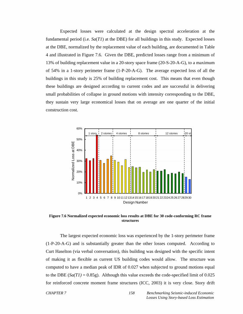
CHAPTER 7 158 Benchmarking Seismic-induced Economic Losses Using Story-based Loss Estimation
Expected losses were calculated at the design spectral acceleration at the
fundamental period (i.e. Sa(T1) at the DBE) for all buildings in this study. Expected losses
at the DBE, normalized by the replacement value of each building, are documented in Table
4 and illustrated in Figure 7.6. Given the DBE, predicted losses range from a minimum of
13% of building replacement value in a 20-story space frame (20-S-20-A-G), to a maximum
of 54% in a 1-story perimeter frame (1-P-20-A-G). The average expected loss of all the
buildings in this study is 25% of building replacement cost. This means that even though
these buildings are designed according to current codes and are successful in delivering
small probabilities of collapse in ground motions with intensity corresponding to the DBE,
they sustain very large economical losses that on average are one quarter of the initial
construction cost.
0%
10%
20%
30%
40%
50%
60%
1 2 3 4 5 6 7 8 9 10111213141516171819 202122232425 2627282930
Design Number
No
rma
lize
d L
oss
at D
BE
1 story 2 stories 4 stories 8 stories 12 stories 20 st
0%
10%
20%
30%
40%
50%
60%
1 2 3 4 5 6 7 8 9 10111213141516171819 202122232425 2627282930
Design Number
No
rma
lize
d L
oss
at D
BE
1 story 2 stories 4 stories 8 stories 12 stories 20 st
Figure 7.6 Normalized expected economic loss results at DBE for 30 code-conforming RC frame structures
The largest expected economic loss was experienced by the 1-story perimeter frame
(1-P-20-A-G) and is substantially greater than the other losses computed. According to
Curt Haselton (via verbal conversation), this building was designed with the specific intent
of making it as flexible as current US building codes would allow. The structure was
computed to have a median peak of IDR of 0.027 when subjected to ground motions equal
to the DBE (Sa(T1) = 0.85g). Although this value exceeds the code-specified limit of 0.025
for reinforced concrete moment frame structures (ICC, 2003) it is very close. Story drift

CHAPTER 7 159 Benchmarking Seismic-induced Economic Losses Using Story-based Loss Estimation
demands are often computed in design using equivalent static methods, and this building
does meet those requirements using this procedure according to Haselton and Deierlein
(2007). As a result, this building experiences large values of peak IDR at very small ground
motion intensity levels. For example, a median IDR of 0.011 is computed at an Sa(T1) =
0.35g, which is large enough to induce structural damage. These large drifts will result in
large estimations of damage and monetary loss as demonstrated by Figure 7.6. This design
may be unconventional and not necessarily representative of what is commonly constructed.
Therefore, it can be considered an outlier and removed when computing statistics on the
loss results. If this building is excluded, the mean expected loss for this set of buildings
reduces to 24%. Despite the fact that this building can be considered unconventional, it is
important to note that it still meets code requirements and was analyzed to demonstrate the
level of inconsistent performance that code may allow.
Haselton and Deierlein (2007) found that of all the design parameters, building
height had the largest influence on collapse safety. Similarly, results from this investigation
indicate that building height also has a significant influence on economic losses. Figure
7.7(a) shows the normalized loss vulnerability curves for 2, 4, 8, 12 and 20-story space
frames (2-S-20-A-G, 4-S-20-A-G, 8-S-20-A-G, 12-S-20-A-G and 20-S-20-A-G), and
Figure 7.7(b) plots the curves of perimeter frames for those corresponding heights (2-P-20-
A-G, 4-P-20-A-G, 8-P-20-A-G, 12-P-20-A-G and 20-P-20-A-G). It is shown that losses
normalized by the replacement cost of the building tend to decrease as the height of the
building increases (this trend is particularly apparent at higher ground motion intensities).
Expected loss at the DBE is plotted as a function of building height in Figure 7.7(c) for both
space and perimeter frame structures. Lower normalized losses are observed in taller
buildings because in moment frame buildings higher drift demands concentrate in a smaller
percentage of the height, while the shorter buildings’ drifts are more evenly distributed as
shown in Figure 7.7(d). Concentration of interstory drift demands typically increase as the
level of ground motion intensity increase and therefore the influence of height increases as
the ground motion increases. Consequently, damage and normalized loss will also be
concentrated in a smaller amount of floors in taller buildings, and produce a smaller
percentage of loss relative to the replacement cost of the building. This trend is more
pronounced in perimeter frames because soft story mechanisms are more likely to form in
these types of structures. While concentration of lateral deformations is considered
undesirable in terms of collapse because collapse may be triggered earlier, the concentration
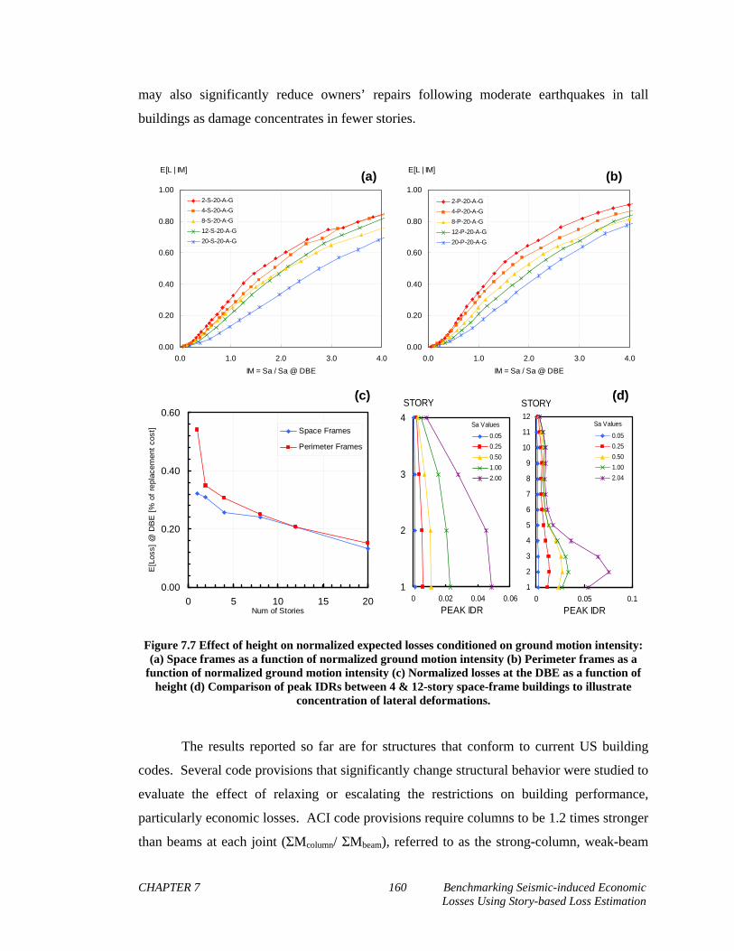
CHAPTER 7 160 Benchmarking Seismic-induced Economic Losses Using Story-based Loss Estimation
may also significantly reduce owners’ repairs following moderate earthquakes in tall
buildings as damage concentrates in fewer stories.
0.00
0.20
0.40
0.60
0.80
1.00
0.0 1.0 2.0 3.0 4.0
IM = Sa / Sa @ DBE
E[L | IM]
2-P-20-A-G
4-P-20-A-G
8-P-20-A-G
12-P-20-A-G
20-P-20-A-G
0.00
0.20
0.40
0.60
0 5 10 15 20Num of Stories
E[L
oss]
@ D
BE
[%
of
repl
acem
ent
cost
] Space Frames
Perimeter Frames
1
2
3
4
0 0.02 0.04 0.06
PEAK IDR
0.05
0.25
0.50
1.00
2.00
STORY
Sa Values
0.00
0.20
0.40
0.60
0.80
1.00
0.0 1.0 2.0 3.0 4.0
IM = Sa / Sa @ DBE
E[L | IM]
2-S-20-A-G
4-S-20-A-G
8-S-20-A-G
12-S-20-A-G
20-S-20-A-G
1
2
3
4
5
6
7
8
9
10
11
12
0 0.05 0.1
PEAK IDR
0.05
0.25
0.50
1.00
2.04
STORY
Sa Values
(a) (b)
(c) (d)
0.00
0.20
0.40
0.60
0.80
1.00
0.0 1.0 2.0 3.0 4.0
IM = Sa / Sa @ DBE
E[L | IM]
2-P-20-A-G
4-P-20-A-G
8-P-20-A-G
12-P-20-A-G
20-P-20-A-G
0.00
0.20
0.40
0.60
0 5 10 15 20Num of Stories
E[L
oss]
@ D
BE
[%
of
repl
acem
ent
cost
] Space Frames
Perimeter Frames
1
2
3
4
0 0.02 0.04 0.06
PEAK IDR
0.05
0.25
0.50
1.00
2.00
STORY
Sa Values
0.00
0.20
0.40
0.60
0.80
1.00
0.0 1.0 2.0 3.0 4.0
IM = Sa / Sa @ DBE
E[L | IM]
2-S-20-A-G
4-S-20-A-G
8-S-20-A-G
12-S-20-A-G
20-S-20-A-G
1
2
3
4
5
6
7
8
9
10
11
12
0 0.05 0.1
PEAK IDR
0.05
0.25
0.50
1.00
2.04
STORY
Sa Values
(a) (b)
(c) (d)
Figure 7.7 Effect of height on normalized expected losses conditioned on ground motion intensity: (a) Space frames as a function of normalized ground motion intensity (b) Perimeter frames as a
function of normalized ground motion intensity (c) Normalized losses at the DBE as a function of height (d) Comparison of peak IDRs between 4 & 12-story space-frame buildings to illustrate
concentration of lateral deformations.
The results reported so far are for structures that conform to current US building
codes. Several code provisions that significantly change structural behavior were studied to
evaluate the effect of relaxing or escalating the restrictions on building performance,
particularly economic losses. ACI code provisions require columns to be 1.2 times stronger
than beams at each joint (ΣMcolumn/ ΣMbeam), referred to as the strong-column, weak-beam

CHAPTER 7 161 Benchmarking Seismic-induced Economic Losses Using Story-based Loss Estimation
ratio (SCWB), to diminish the possibility of plastic hinging in the columns. Haselton and
Deierlein (2007) demonstrated that this ratio has a significant influence on structural
collapse capacity. In this study the influence of the SCWB ratio on economic losses was
investigated. The variation of economic losses normalized by the replacement value as a
function of the level of ground motion intensity of four-story structures designed with
SCWB ratios of 0.4, 0.6, 0.8, 1.0, 1.2, 1.5, 2.0 and 3.0 are shown in Figure 7.8(a). Figure
7.8(b) shows the influence of SCWB ratio of the normalized loss in the DBE event, which
are also disaggregated to show the contributions from collapse and non-collapse losses.
0.00
0.10
0.20
0.30
0.40
0.50
0.4 0.6 0.8 1.0 1.2 1.5 2.0 3.0
Strong-Col, Weak-Bm Ratio
Non-Collapse
Collapse
E[L | IM = Sa @ DBE]
0.00
0.20
0.40
0.60
0.80
1.00
0.0 1.0 2.0 3.0 4.0
IM = Sa / Sa @ DBE
E[L | IM]
4S30AG - SCWB = 0.44S30AG - SCWB = 0.64S30AG - SCWB = 0.84S30AG - SCWB = 1.04S30AG - SCWB = 1.24S30AG - SCWB = 1.54S30AG - SCWB = 2.04S30AG - SCWB = 3.0
(a) (b)
0.00
0.10
0.20
0.30
0.40
0.50
0.4 0.6 0.8 1.0 1.2 1.5 2.0 3.0
Strong-Col, Weak-Bm Ratio
Non-Collapse
Collapse
E[L | IM = Sa @ DBE]
0.00
0.20
0.40
0.60
0.80
1.00
0.0 1.0 2.0 3.0 4.0
IM = Sa / Sa @ DBE
E[L | IM]
4S30AG - SCWB = 0.44S30AG - SCWB = 0.64S30AG - SCWB = 0.84S30AG - SCWB = 1.04S30AG - SCWB = 1.24S30AG - SCWB = 1.54S30AG - SCWB = 2.04S30AG - SCWB = 3.0
(a) (b)
Figure 7.8 Effect of strong-column, weak-beam ratio on: (a) normalized expected loss as a function of normalized ground motion intensity (b) normalized expected loss at the DBE, disaggregated by
collapse & non-collapse losses.
Both figures demonstrate that SCWB ratios of 0.4 and 0.6 have larger economic
losses because of the higher probability of collapse in these cases. While the losses due to
collapse significantly decrease as the SCWB ratio increases, the total losses remain
approximately the same (~23-26%) for ratios greater than 0.8. In buildings with small
SCWB ratios column hinging occurs early and produces collapse mechanism in one story
and the probability of collapse increases. Since column hinging results in concentration of
lateral deformation demands in 1 or 2 stories, non-collapse losses are smaller and the total
losses are smaller and the total losses are dominated by collapse losses. Although
increasing the SCWB ratio reduces the probability of collapse by preventing hinging in the

CHAPTER 7 162 Benchmarking Seismic-induced Economic Losses Using Story-based Loss Estimation
columns, lateral deformation in these structures become more evenly distributed along the
height resulting in more nonstructural damage. While increasing the SCWB ratio to a value
greater than 1.2 could potentially have a substantial impact on collapse performance (and
perhaps life safety), it does not appear to help mitigate economic losses.
The strength reduction factor, R, (ASCE-05, 2005) which is used to calculate a
structure’s design base shear, demonstrated a larger influence on total expected losses than
the SCWB ratio. Loss results for structures with R = 4, R = 8 and R = 10 are shown in
Figure 7.9. These structures have design base shear coefficients (Cs = V/W) of 0.077, 0.044
and 0.028, respectively. When designed for a small base shear, structures become weaker
and more flexible and the losses incurred are higher. At the DBE, increasing the R-factor
from 8 to 10 increases the expected losses by 25%. On the other hand, decreasing the R-
factor from 8 to 4, leads to a 12% decrease in expected loss at the DBE. These results
suggests that there is a disincentive to relaxing the seismic design force by increasing R,
due to a predicted increase in economic losses. Decreasing R and increasing the design
base shear has the opposite effect, reducing economic losses, but the impact is less
significant.
0.00
0.20
0.40
0.60
0.80
1.00
0.0 1.0 2.0 3.0 4.0
IM = Sa / Sa @ DBE
E[L | IM]
R=4
R=8
R=10
Figure 7.9 Effect of design base shear on normalized expected loss as a function of ground motion intensity
The other design parameters considered in this study had minimal influence on
expected losses. Structures that maintained uniform strength and stiffness of structural
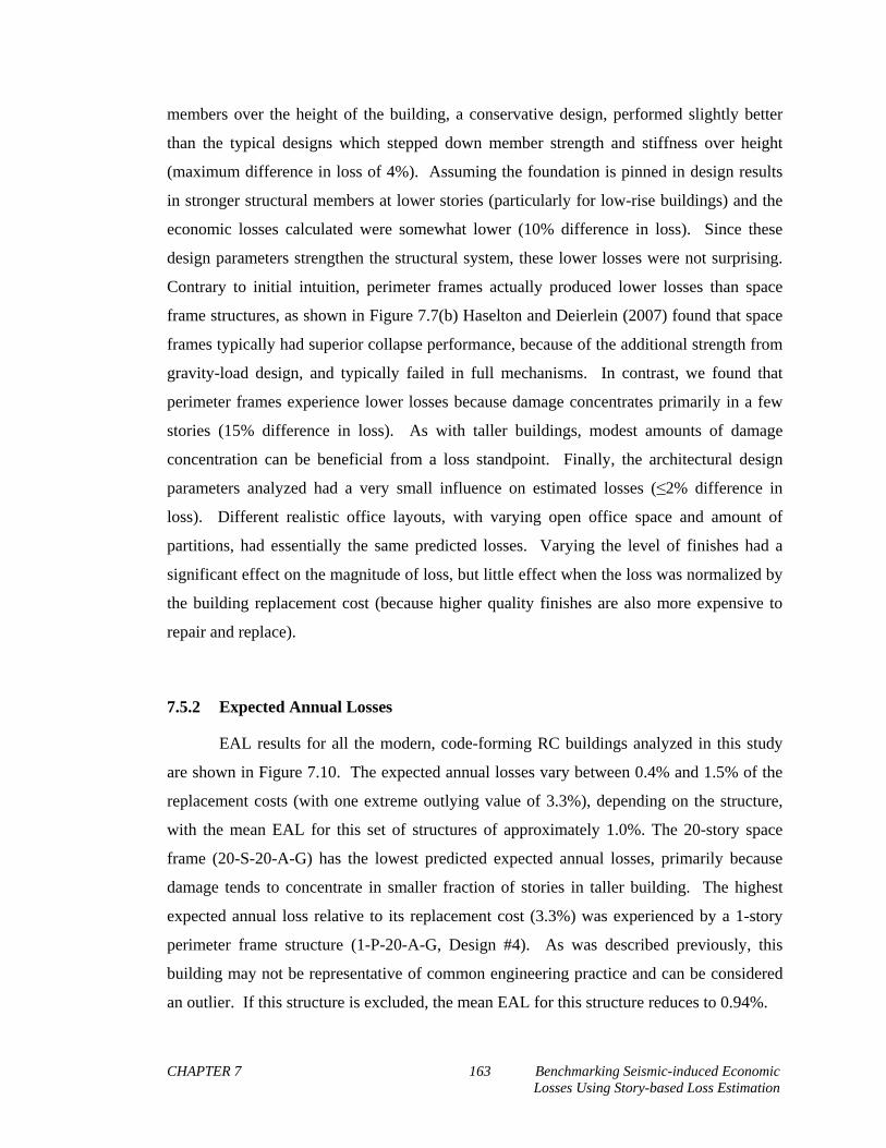
CHAPTER 7 163 Benchmarking Seismic-induced Economic Losses Using Story-based Loss Estimation
members over the height of the building, a conservative design, performed slightly better
than the typical designs which stepped down member strength and stiffness over height
(maximum difference in loss of 4%). Assuming the foundation is pinned in design results
in stronger structural members at lower stories (particularly for low-rise buildings) and the
economic losses calculated were somewhat lower (10% difference in loss). Since these
design parameters strengthen the structural system, these lower losses were not surprising.
Contrary to initial intuition, perimeter frames actually produced lower losses than space
frame structures, as shown in Figure 7.7(b) Haselton and Deierlein (2007) found that space
frames typically had superior collapse performance, because of the additional strength from
gravity-load design, and typically failed in full mechanisms. In contrast, we found that
perimeter frames experience lower losses because damage concentrates primarily in a few
stories (15% difference in loss). As with taller buildings, modest amounts of damage
concentration can be beneficial from a loss standpoint. Finally, the architectural design
parameters analyzed had a very small influence on estimated losses (≤2% difference in
loss). Different realistic office layouts, with varying open office space and amount of
partitions, had essentially the same predicted losses. Varying the level of finishes had a
significant effect on the magnitude of loss, but little effect when the loss was normalized by
the building replacement cost (because higher quality finishes are also more expensive to
repair and replace).
7.5.2 Expected Annual Losses
EAL results for all the modern, code-forming RC buildings analyzed in this study
are shown in Figure 7.10. The expected annual losses vary between 0.4% and 1.5% of the
replacement costs (with one extreme outlying value of 3.3%), depending on the structure,
with the mean EAL for this set of structures of approximately 1.0%. The 20-story space
frame (20-S-20-A-G) has the lowest predicted expected annual losses, primarily because
damage tends to concentrate in smaller fraction of stories in taller building. The highest
expected annual loss relative to its replacement cost (3.3%) was experienced by a 1-story
perimeter frame structure (1-P-20-A-G, Design #4). As was described previously, this
building may not be representative of common engineering practice and can be considered
an outlier. If this structure is excluded, the mean EAL for this structure reduces to 0.94%.

CHAPTER 7 164 Benchmarking Seismic-induced Economic Losses Using Story-based Loss Estimation
0.0%
0.5%
1.0%
1.5%
2.0%
2.5%
3.0%
3.5%
4.0%
1 2 3 4 5 6 7 8 9 101112131415161718192021222324252627282930
Design Number
No
rma
lized
Exp
ecte
d A
nnua
l Lo
ss
1 story 2 stories 4 stories 8 stories 12 stories 20 st
0.0%
0.5%
1.0%
1.5%
2.0%
2.5%
3.0%
3.5%
4.0%
1 2 3 4 5 6 7 8 9 101112131415161718192021222324252627282930
Design Number
No
rma
lized
Exp
ecte
d A
nnua
l Lo
ss
1 story 2 stories 4 stories 8 stories 12 stories 20 st
0.0%
0.5%
1.0%
1.5%
2.0%
2.5%
3.0%
3.5%
4.0%
1 2 3 4 5 6 7 8 9 101112131415161718192021222324252627282930
Design Number
No
rma
lized
Exp
ecte
d A
nnua
l Lo
ss
1 story 2 stories 4 stories 8 stories 12 stories 20 st
Figure 7.10 EAL results for 30 code-conforming RC frame structures
Multiple measures of seismic performance are useful when comparing design
alternatives. Figure 7.11 shows the mean annual frequency of collapse for the set of RC
structures as calculated by Haselton and Deierlein (2007). The mean annual frequency of
collapse corresponds approximately to the probability of collapse in a given year, and is an
important metric for life safety. It is clear by comparing Figure 7.10 and Figure 7.11, and
referring to Figure 7.12, that understanding how likely a building is to collapse provides
little information on the value of EAL that building may experience. Design 8-P-20-A-G
(Design #14 in the figure), an 8-story perimeter frame building, has the worst collapse
performance, but its EAL is nearly average for the group of RC frame structures. Figure
7.12 confirms that there is not a strong relationship between EAL and the mean annual
frequency of collapse (correlation coefficient, = -0.40). These observations suggest that
increasing collapse capacity does not necessarily mitigate economic losses and that
consideration of economic losses, need to be addressed separately from collapse.

CHAPTER 7 165 Benchmarking Seismic-induced Economic Losses Using Story-based Loss Estimation
0
5
10
15
20
25
30
1 2 3 4 5 6 7 8 9 10 1112 1314 1516 1718 1920 2122 232425 2627 2829 30
Design Number
MA
F C
olla
pse
x 1
0-4
1 story 2 stories 4 stories 8 stories 12 stories 20 st
0
5
10
15
20
25
30
1 2 3 4 5 6 7 8 9 10 1112 1314 1516 1718 1920 2122 232425 2627 2829 30
Design Number
MA
F C
olla
pse
x 1
0-4
1 story 2 stories 4 stories 8 stories 12 stories 20 st
Figure 7.11 Results of mean annual frequency of collapse for 30 code-conforming RC frame structures (Haselton and Deierlein, 2007).
Performance-based approaches enable consideration of multiple seismic
performance metrics in design. Modern building codes aim to protect life-safety by
reducing the risk of collapse, but these goals do not necessarily translate into good
performance in terms of limiting economic loss. The weak relationship between critical
code design parameters and economic losses is further evident when collapse and loss
metrics are compared to the structural strength of the buildings. Figure 7.12(b) and (c) plots
MAF of collapse and EAL, respectively, as a function of the yield base shear coefficient
from a nonlinear pushover analysis. As expected, there is a relatively strong negative
correlation (ρ=-0.66) between MAF of collapse and the yield base shear coefficient because
collapse is less likely in stronger structures. The weak correlation (ρ=0.42) between EAL
and the yield base shear suggests that strength is not the only design parameter that needs to
be addressed by codes to mitigate large economic losses. This type of information is
important for stakeholders who are making design decisions to protect their investment.
The use of performance-based tools in this study illustrates how this framework is useful to
address both life-safety and economic loss in ways current code approaches cannot.

CHAPTER 7 166 Benchmarking Seismic-induced Economic Losses Using Story-based Loss Estimation
0.0%
0.4%
0.8%
1.2%
1.6%
0 10 20 30
MAF Collapse (x10-4)
EAL
=-0.41
(a)
0.0%
0.4%
0.8%
1.2%
1.6%
0 10 20 30
MAF Collapse (x10-4)
EAL
=-0.41
(a)
0
5
10
15
20
25
30
0.0 0.2 0.4 0.6
Yield Base Shear Coefficient
= -0.66
MAF Collapse (x10-4) (b)
0
5
10
15
20
25
30
0.0 0.2 0.4 0.6
Yield Base Shear Coefficient
= -0.66
MAF Collapse (x10-4) (b)
0.0%
0.4%
0.8%
1.2%
1.6%
0.0 0.2 0.4 0.6
Yield Base Shear Coefficient
EAL
= 0.42
(c)
0.0%
0.4%
0.8%
1.2%
1.6%
0.0 0.2 0.4 0.6
Yield Base Shear Coefficient
EAL
= 0.42
(c)
Figure 7.12 Scatter plots and correlation coefficients between: (a) EAL & MAF of collapse (b) MAF of collapse & yield base shear coefficient (c) EAL & yield base shear coefficient
7.5.3 Present value of life-cycle costs
Another way of putting these results into a more understandable context, is to
evaluate the present value of the losses over a building’s typical lifespan. Expected Annual
Losses, like those shown in Figure 7.10, can be annualized over a period of time to give
insight on the life-cycle costs associated with earthquake damage. In this study, a
building’s life-span was taken to be 50 years. Each structure’s EAL was multiplied by this
expected lifetime and discounted to obtain the equivalent present value of 50 years of
losses, as shown in Figure 7.13(a) with a discount rate of 3%. For these code-conforming
structures present values of life cycle costs of earthquake damage range from 11% to 85%
of the total replacement value of the structure. Because the discount rate may vary, this

CHAPTER 7 167 Benchmarking Seismic-induced Economic Losses Using Story-based Loss Estimation
calculation was repeated for a variety of discount rates for the buildings with the minimum
and maximum present value of expected loss, as shown in Figure 7.13(b). Note that design
number 4 is considered as an extreme case and is not included in the calculation for Figure
7.13(b).
0%
20%
40%
60%
80%
100%
1 2 3 4 5 6 7 8 9 1011121314151617 18 1920 21 222324252627282930
Design Number
No
rma
lize
d P
V o
f Lo
sse
s o
ver
50
yrs 1 story 2 stories 4 stories 8 stories 12 stories 20 st
(ass
umin
g a
disc
ount
rat
e of
3%
)
(a)
(b)
0%
10%
20%
30%
40%
50%
60%
70%
80%
0% 1% 2% 3% 4% 5% 6%
Discount Rate
PV
of
Exp
ect
ed
Los
s o
ver
50
yea
rs Max PV of Exp Loss (Bldg. 12)
Min PV of Exp Loss (Bldg. 30)
0%
20%
40%
60%
80%
100%
1 2 3 4 5 6 7 8 9 1011121314151617 18 1920 21 222324252627282930
Design Number
No
rma
lize
d P
V o
f Lo
sse
s o
ver
50
yrs 1 story 2 stories 4 stories 8 stories 12 stories 20 st
(ass
umin
g a
disc
ount
rat
e of
3%
)
(a)
(b)
0%
20%
40%
60%
80%
100%
1 2 3 4 5 6 7 8 9 1011121314151617 18 1920 21 222324252627282930
Design Number
No
rma
lize
d P
V o
f Lo
sse
s o
ver
50
yrs 1 story 2 stories 4 stories 8 stories 12 stories 20 st
(ass
umin
g a
disc
ount
rat
e of
3%
)
0%
20%
40%
60%
80%
100%
1 2 3 4 5 6 7 8 9 1011121314151617 18 1920 21 222324252627282930
Design Number
No
rma
lize
d P
V o
f Lo
sse
s o
ver
50
yrs 1 story 2 stories 4 stories 8 stories 12 stories 20 st
(ass
umin
g a
disc
ount
rat
e of
3%
)
(a)
(b)
0%
10%
20%
30%
40%
50%
60%
70%
80%
0% 1% 2% 3% 4% 5% 6%
Discount Rate
PV
of
Exp
ect
ed
Los
s o
ver
50
yea
rs Max PV of Exp Loss (Bldg. 12)
Min PV of Exp Loss (Bldg. 30)
0%
10%
20%
30%
40%
50%
60%
70%
80%
0% 1% 2% 3% 4% 5% 6%
Discount Rate
PV
of
Exp
ect
ed
Los
s o
ver
50
yea
rs Max PV of Exp Loss (Bldg. 12)
Min PV of Exp Loss (Bldg. 30)
0%
10%
20%
30%
40%
50%
60%
70%
80%
0% 1% 2% 3% 4% 5% 6%
Discount Rate
PV
of
Exp
ect
ed
Los
s o
ver
50
yea
rs Max PV of Exp Loss (Bldg. 12)
Min PV of Exp Loss (Bldg. 30)
Figure 7.13 Present value of normalized economic losses over 50 years for 30 code-conforming RC frame structures: (a) Present value of losses for each building at a discount rate of 3% (b) Range of
present value of losses as a function of discount rate (excluding design number 4).
Figure 7.13(b) gives a likely range where present value of expected losses are likely
to be for buildings designed according to present code. This figure highlights two
important things: (1) the range of losses over buildings that are expected to have similar
performance, may end up varying by a factor as high as three, and (2) the losses are fairly
large (ranging from 11% to 36% at a discount of 3%). Assuming the discount rate of 3%,
stakeholders may lose up to 36% of their initial investment due to future earthquakes.

CHAPTER 7 168 Benchmarking Seismic-induced Economic Losses Using Story-based Loss Estimation
These losses are significant and may not be acceptable to stakeholders, even though these
buildings meet current code requirements. Considering that the structural system is
typically between 15 to 20% of the total initial construction cost (RS Means, 2007), the
additional cost of investing in a lateral resisting system could be worthwhile, compared to
the high life-cycle costs due to earthquakes. Performance-based design tools can be used to
communicate these types of concerns to building owners and other stakeholders.
7.5.4 Comparison to Non-ductile Reinforced Concrete Frame Buildings
Measuring performance in terms of economic losses can be used to quantify how
well changes in US building code provisions over the past 50 years have improved the
seismic design of reinforced concrete moment frame structures. Older reinforced concrete
buildings typically exhibit non-ductile behavior primarily because the reinforcing detailing
requirements were less stringent in previous editions of US building codes (Moehle, 1998).
Smaller amounts of shear reinforcement in beams, columns and joints in these frames
reduce the deformation capacity of these elements and make them more likely to experience
non-ductile failures (Scott et al., 1982). Discontinuous reinforcing through structural joints
and insufficient lap splices may also increase the likelihood of inadequate load transfer
between structural elements, which could lead to loss of vertical carrying capacity. These
types of structural deficiencies increase the probability of damage to structural components
and the probability of collapse that may lead to larger economic losses than those sustained
by modern buildings.
Liel and Deierlein (2008) investigated the seismic performance of non-ductile
reinforced concrete moment frame structures to benchmark these types of structures’
capacity to resist collapse. A set of 26 typical structures (archetypes) were designed, using
the 1967 Uniform Building Code, to be representative of older reinforced concrete moment
frame buildings in California built between 1950 and 1975. Similar modeling and structural
analysis techniques were use as described in section 7.4.2 to assess the collapse capacities
of each building (interested readers are directed to Liel and Deierlein, 2008, for further
details on the procedure and results of this investigation).
Economic loss results were computed for this set of non-ductile structures and use
to compare their performance with the modern, ductile structures created by Haselton and
Deierlein (2007). Figure 7.14(a) compares normalized economic losses conditioned on the

CHAPTER 7 169 Benchmarking Seismic-induced Economic Losses Using Story-based Loss Estimation
ground motion intensity corresponding to the DBE between non-ductile and ductile frames
for 2, 4, 8, and 12 space and perimeter frames. Only the baseline structures for each
building height are considered in this comparison. The economic losses for the non-ductile
structures range from 42% to 71% of the building’s replacement value with median value of
61%. Comparatively, the ductile structures’ normalized losses at the DBE range from 21%
to 35% with a median value of 25%. Normalized EAL results were also computed and
compared in Figure 7.14(b). The normalized EAL of the non-ductile structures range from
1.1% to 3.4%, with a median of 2.6%, whereas the ductile structures varied from 0.7% to
1.3% and has a median of 1.1%. In both types of loss metrics, the median economic losses
of the older, non-ductile structures are 1.4 times greater than those of the modern buildings.
This means that implementing better detailing requirements that increase structural
deformation capacity, not only reduces the probability of collapse, as demonstrated by Liel
and Deierlein (2008), but also significantly reduces economic losses.
0%
20%
40%
60%
80%
100%
2-story 4-story 8-story 12-story 2-story 4-story 8-story 12-story
No
rmal
ized
Lo
ss a
t DB
E
PerimeterSpace
Non-ductile (1967) Ductile (2003)
0%
2%
4%
6%
8%
10%
2-story 4-story 8-story 12-story 2-story 4-story 8-story 12-story
Nor
mal
ized
Exp
ecte
d A
nnua
l Los
s
PerimeterSpace
Non-ductile (1967) Ductile (2003)
(a)
(b)
0%
20%
40%
60%
80%
100%
2-story 4-story 8-story 12-story 2-story 4-story 8-story 12-story
No
rmal
ized
Lo
ss a
t DB
E
PerimeterSpace
Non-ductile (1967) Ductile (2003)
0%
2%
4%
6%
8%
10%
2-story 4-story 8-story 12-story 2-story 4-story 8-story 12-story
Nor
mal
ized
Exp
ecte
d A
nnua
l Los
s
PerimeterSpace
Non-ductile (1967) Ductile (2003)
(a)
(b)
Figure 7.14 Comparison between normalized economic loss results between modern, ductile (2003) and older, non-ductile reinforce concrete frame structures: (a) Expected loss at DBE (b) EAL

CHAPTER 7 170 Benchmarking Seismic-induced Economic Losses Using Story-based Loss Estimation
Figure 7.15 compares the disaggregation of EALs into collapse and non-collapse
losses for the 4-story perimeter frame structures. The non-ductile structure’s losses due to
collapse comprise 28% of the total EAL, whereas only 3% of the ductile structure’s EAL is
attributed to collapse. This suggests that collapse plays a larger role in economic loss for
older buildings, which have higher probabilities of collapse. It can be inferred that
introducing ductile detailing has been successful in reducing the likelihood of collapse and
the monetary losses associated with it. However, the results for modern buildings have
shown that the economic losses are still very large, and are primarily due to non-collapse
losses. Any attempt to mitigate losses further in these building would need to focus on
limiting interstory drifts and floor accelerations rather than other parameters that primarily
associated with preventing collapse .
Collpase28%
Non-Collapse
72%
Collpase3%
Non-Collapse
97%
Non-ductile (1967) Ductile (2003)
EAL Dissaggregation: 4-story perimeter frames
Collpase28%
Non-Collapse
72%
Collpase3%
Non-Collapse
97%
Non-ductile (1967) Ductile (2003)
EAL Dissaggregation: 4-story perimeter frames
Figure 7.15 Comparison of EAL disaggregation of collapse and non-collapse losses for non-ductile and ductile frames
7.5.5 Loss Toolbox Comparison
Previous loss estimation methods have relied heavily on expert opinion and
engineering judgment, making the results open to subjectivity (Aslani and Miranda, 2005).
One of the goals of PEER’s building-specific loss methodologies is to establish a
framework that is rational and generates vulnerability curves from data that is well-
documented. It is also important that the methodology produces results that are consistent
and robust given the same input data and parameters. Mitrani-Reiser and Beck (2007)
developed a computer tool, the MATLAB Damage and Loss Analysis (MLDA) toolbox,

CHAPTER 7 171 Benchmarking Seismic-induced Economic Losses Using Story-based Loss Estimation
that implements PEER’s component-based loss estimation framework. MLDA was used to
in a previous study (Ramirez et al., 2009) to estimate expected losses for the same set of 30
code-conforming reinforced concrete moment frame office buildings developed by
Haselton and Deierlein (2007), so that they could be compared to the results produced by
the simplified, story-based loss estimation methods used in this study. The results were
compared to identify any discrepancies and the sources of the inconsistencies.
Figure 7.16 compares vulnerability curves produced by this study (solid lines) to
those generated from MDLA (dashed lines). In Figure 7.16(a), the perimeter frame results
appear to be relatively consistent between the two approaches. The curves for space
frames, shown in Figure 7.16(b), demonstrate greater discrepancies between the results of
the two toolboxes. The differences can be attributed to the way the losses due to non-
collapse are formulated.
0.00
0.20
0.40
0.60
0.80
1.00
0.0 1.0 2.0 3.0
IM = Sa / Sa @ DBE
E[L | IM]
Space Frames0.00
0.20
0.40
0.60
0.80
1.00
0.0 1.0 2.0 3.0
IM = Sa / Sa @ DBE
E[L | IM]
1-Story
2-Story
4-Story
8-Story
12-Story
20-Story
Perimeter Frames
(a) (b)
Solid Lines: This study
Dashed Lines: MLDA
0.00
0.20
0.40
0.60
0.80
1.00
0.0 1.0 2.0 3.0
IM = Sa / Sa @ DBE
E[L | IM]
Space Frames0.00
0.20
0.40
0.60
0.80
1.00
0.0 1.0 2.0 3.0
IM = Sa / Sa @ DBE
E[L | IM]
1-Story
2-Story
4-Story
8-Story
12-Story
20-Story
Perimeter Frames
(a) (b)
Solid Lines: This study
Dashed Lines: MLDA
Figure 7.16 Comparison of vulnerability curves from this study and from MDLA: (a) perimeter frames (b) space frames
The collapse losses in both approaches are identical because the main equation to
compute these losses (Chapter 3, equation 3.2) and the parameters that go into the equation,
the building replacement costs and collapse fragilities, are the same. Therefore, the way
non-collapse losses are computed can be the only source of discrepancy. The space frames
exhibit larger differences in estimations between the two approaches because the non-
collapse losses play a larger role in the overall losses. Space frames have lower
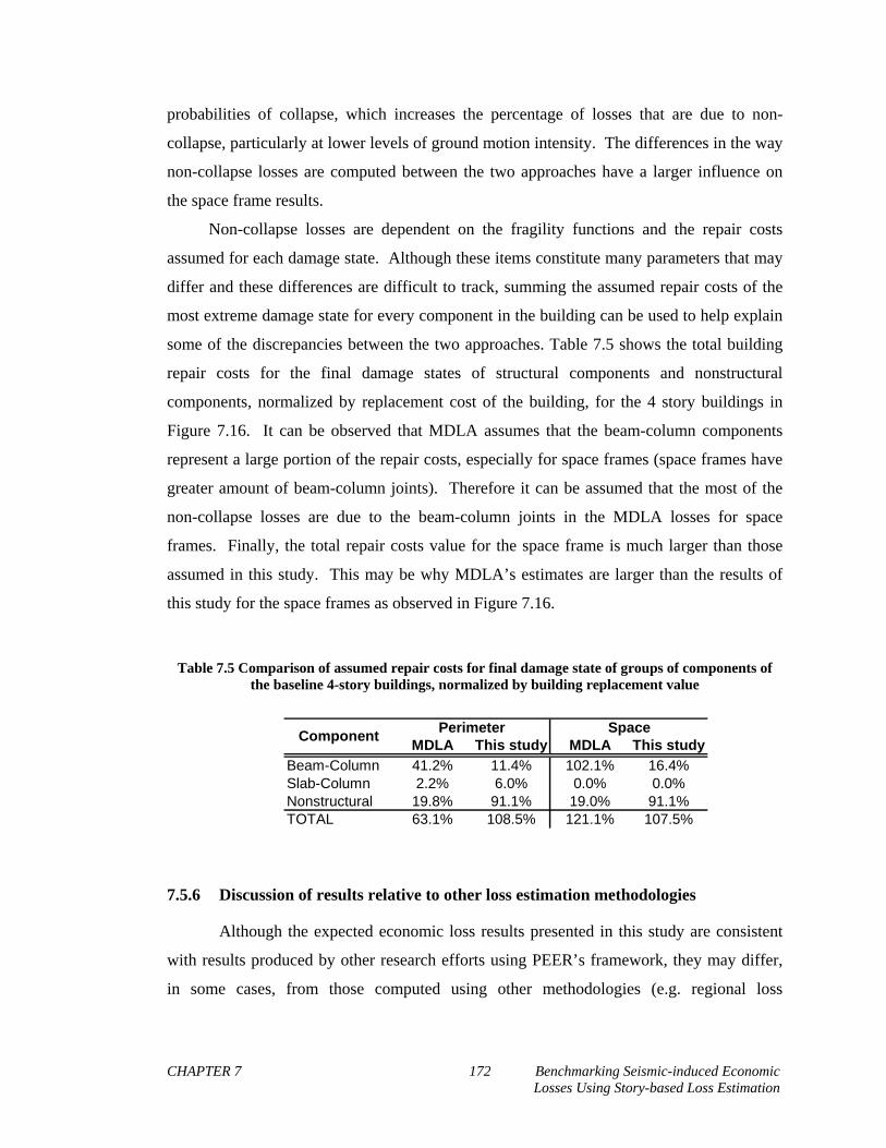
CHAPTER 7 172 Benchmarking Seismic-induced Economic Losses Using Story-based Loss Estimation
probabilities of collapse, which increases the percentage of losses that are due to non-
collapse, particularly at lower levels of ground motion intensity. The differences in the way
non-collapse losses are computed between the two approaches have a larger influence on
the space frame results.
Non-collapse losses are dependent on the fragility functions and the repair costs
assumed for each damage state. Although these items constitute many parameters that may
differ and these differences are difficult to track, summing the assumed repair costs of the
most extreme damage state for every component in the building can be used to help explain
some of the discrepancies between the two approaches. Table 7.5 shows the total building
repair costs for the final damage states of structural components and nonstructural
components, normalized by replacement cost of the building, for the 4 story buildings in
Figure 7.16. It can be observed that MDLA assumes that the beam-column components
represent a large portion of the repair costs, especially for space frames (space frames have
greater amount of beam-column joints). Therefore it can be assumed that the most of the
non-collapse losses are due to the beam-column joints in the MDLA losses for space
frames. Finally, the total repair costs value for the space frame is much larger than those
assumed in this study. This may be why MDLA’s estimates are larger than the results of
this study for the space frames as observed in Figure 7.16.
Table 7.5 Comparison of assumed repair costs for final damage state of groups of components of the baseline 4-story buildings, normalized by building replacement value
MDLA This study MDLA This study
Beam-Column 41.2% 11.4% 102.1% 16.4%Slab-Column 2.2% 6.0% 0.0% 0.0%Nonstructural 19.8% 91.1% 19.0% 91.1%TOTAL 63.1% 108.5% 121.1% 107.5%
Perimeter SpaceComponent
7.5.6 Discussion of results relative to other loss estimation methodologies
Although the expected economic loss results presented in this study are consistent
with results produced by other research efforts using PEER’s framework, they may differ,
in some cases, from those computed using other methodologies (e.g. regional loss
CHAPTER 7 173 Benchmarking Seismic-induced Economic Losses Using Story-based Loss Estimation
estimation methods, proprietary models in the insurance industry,…etc.). There are several
possible reasons for differences in estimating losses, which are described briefly here.
There may be differences in the way damage is estimated. The fragility functions
used in this study are updated functions that have been developed in the past few years.
These functions may differ from those used by previous loss estimation methods, as was
demonstrated in Chapter 5. The generic fragility functions used to estimate damage for a
large portion of drift-sensitive, nonstructural components in this study were compared to
those used by HAZUS. It was determined that the functions used in this study estimate that
damage will initiate at smaller values than those approximated by the HAZUS functions.
This may result in loss estimations that will be higher than those computed by HAZUS,
given that the displacement demands computed are the same.
The values of displacement demands used to estimate loss may also differ because
the methods of calculating structural response parameters may be different than other
approaches. Many regional loss estimation methods use first-order estimates of structural
response based on single degree of freedom (SDOF) systems such as spectral acceleration
and spectral displacement. The methodology established by PEER uses more complex
structural models to estimate response. The differences in computing structural response
may produce differences in response parameters, which are used to determine losses due to
repair of building components.
Estimation of inelastic displacement by other loss estimation methods is often
computed using equivalent linear methods. This may produce very different displacement
demands than those computed using detailed nonlinear simulation models. As was
observed by the disaggregated results in this study, economic losses in reinforced concrete
moment frame office buildings are largely due to drift-sensitive components. Differing
displacement demands may cause large differences in loss estimations.
Not only are the values of response parameters used in loss estimation dependent on
the way they are computed, they are also dependent on the building properties and
parameters that are estimated. Structural parameters that may have a strong influence on
economic loss estimations include the building’s assumed damping ratio, its estimated
ductility ratio, its height (as was demonstrated earlier in this chapter) and its estimated
fundamental period of vibration. Regional loss estimation methods often group structures
into generic building types and assume that these parameters are the same for structures that
fall under the same type. For instance, HAZUS categorizes modern reinforced concrete
CHAPTER 7 174 Benchmarking Seismic-induced Economic Losses Using Story-based Loss Estimation
moment frame buildings that are designed to current US building code standards (termed
“High-code seismic design level” by HAZUS, and based on code standards established after
1975) into three basic types: low-rise (1-3 stories), mid-rise (4-7 stories) and high-rise (≥8
stories) structures (according to HAZUS terminology, these building types are coded as
C1L, C1M and C1H, respectively). According to the HAZUS technical manual (NIBS,
2003), the fundamental periods estimated for these building types are 0.40s for the low-rise
structures, 0.75s for the mid-rise structures and 1.45s for the high-rise structures. These can
be compared to the periods computed by Haselton and Deierlein (2007) for the set of
buildings analyzed in this study. Table 7.3 reports that the periods for the 1 and 2-story
buildings vary from 0.42s to 0.71s, the periods for the 4-story buildings vary from 0.86s to
1.16s and the buildings for the 8, 12 and 20-story buildings have periods that vary from
1.57s to 2.63s. These values are all larger than the periods assumed by HAZUS for the low-
rise, mid-rise and high-rise building types, respectively. Larger periods (i.e. structures that
are more flexible) will produce larger displacement demands, which will result in larger
economic losses.
The differences between economic loss estimations computed by PEER’s
framework and those produced by other methods may be substantial, depending on the
approach, and need to be studied further. Future studies are required to reconcile these
differences and validate the results presented here.
7.6 LIMITATIONS
In conducting this study, we encountered a variety of challenges in implementing
the PEER methodology for predicting economic losses that warrant further research. These
items include:
In the current study, uncertainties in structural modeling were incorporated in
predictions of the structural collapse limit state, but not the non-collapse EDPs.
These modeling uncertainties represent the uncertainty in how well the model
reflects the true behavior of the structure. Modeling uncertainties have a particularly
important effect in highly nonlinear limit states such as collapse, because these
phenomena are more difficult to model. Previous studies have shown them to be
less significant for smaller levels of structural response that tend to dominate losses
CHAPTER 7 175 Benchmarking Seismic-induced Economic Losses Using Story-based Loss Estimation
(e.g. Porter 2002). A detailed examination of the effects of modeling uncertainties
on predictions of structural losses is a topic for future work.
The collapse fragility is appropriately adjusted to reflect the expected spectral shape
in large, rare ground motions (epsilon > 0) (Baker and Cornell 2005). Because the
smaller ground motions that dominate non-collapse losses are typically closer to
epsilon-neutral, this effect is not included for predictions of non-collapse
engineering response. A more complete approach would account appropriately for
the expected shape of ground motions at each stripe (intensity level). This change is
not expected to have significant effects on the overall results.
Economic losses in this study include only direct economic losses associating with
repairing damageable components. The costs associated with building closure and
the downtime needed to conduct repairs may be an even more significant source of
loss to building owners (Comerio 2006). In future, these studies should include as
many possible sources of economic loss related to seismic damage as possible. By
including all possible sources of economic losses, life cycle costs associated with
earthquakes can be more completely determined and used by building owners in
making important decisions about earthquake investment.
7.7 CONCLUSIONS
PEER’s performance-based earthquake engineering methodology was used to
evaluate economic losses for a set of 30 modern concrete moment frame buildings. All the
buildings were designed -- structurally and architecturally -- to provide a realistic inventory
of damageable components. The structural designs are representative of modern code-
conforming structures and were reviewed by a practicing engineer as part of the Applied
Technology Council Project 63 (ATC 2008). Results from probabilistic seismic hazard
analysis and incremental dynamic analysis performed by previous investigators (Goulet et
al. 2007, Haselton and Deierlein 2007) were used to evaluate the site’s hazard and structural
response respectively. Ramirez and Miranda’s toolbox (2009) was then used to calculate
damage and economic loss, defined as cost of repairing earthquake damage, of each
structure. Seismic performance metrics generated in this study include expected losses
CHAPTER 7 176 Benchmarking Seismic-induced Economic Losses Using Story-based Loss Estimation
conditioned on seismic intensity, expected annual losses, and present values of life cycle
costs associated with repairing earthquake damage.
Expected losses were calculated at several values of intensity, but results at the
DBE in particular were used to identify trends. Losses at this intensity were found to be a
significant percentage of the replacement value, ranging from 13% to 54%. This means that
although current code-conforming buildings have small probabilities of collapse at the DBE
intensity, the economic losses sustained are very large. The mean EAL for this set of
structures is approximately 1.0% of the replacement cost, but varied between 0.4% and
3.3%, suggesting that current US building codes provide an inconsistent level of seismic
performance when considering monetary loss. This set of structures also exhibited life-
cycle costs associated with earthquake damage that ranged from 8% to as much as 37%
over a 50 year period, despite conforming to modern building codes. Like the scenario-
based results for a given level of ground motion intensity, these losses are large and a
considerable amount of the buildings’ initial investment.
Different design parameters, both structure-related and architecture-related, were
varied within the set to examine how they affected performance. Of the code-conforming
structural parameters considered in this study, building height was found to have the largest
influence on expected losses. Taller buildings experienced less relative loss than shorter
buildings because damage concentrates in a small percentage of floors as opposed to
damage throughout all levels of the structure. Structural parameters that explored the effect
of particular code limitations were also investigated. Although increasing the design
SCWB ratio to values greater than one reduced the economic losses due to collapse, it did
not significantly decrease the overall expected losses. On the other hand, modifying the R-
factor had a larger effect on expected losses at the DBE. If code committees are interested
in adjusting code provisions to limit direct economic losses due to seismic ground motions,
this study suggests that they would be best served by making amendments to the R-factor.
Stiffness limitations and the Cd factor are also expected to have significant effects on
economic losses.
It was also demonstrated that designing for life-safety does not necessarily translate
to satisfactory economic loss performance. The parameters of EAL and the MAF of
collapse were found to be uncorrelated for these set of buildings. Performance-based
design tools provide separate quantifiable metrics to address collapse risks and economic
losses. The ability to quantify both metrics also provides decision-makers with information

CHAPTER 7 177 Benchmarking Seismic-induced Economic Losses Using Story-based Loss Estimation
to identify and consider possible tradeoffs between mitigating losses and reducing collapse
risk.
When the modern set of ductile reinforced concrete buildings were compared to a
set of non-ductile frame structures, representative of older buildings in California, it was
determined that these buildings pose an even greater risk with expected losses that were 1.4
times as great. The non-ductile detailing of these older structures make them more
susceptible to sudden, non-ductile structural collapses as reflected by their larger collapse
probabilities. Consequently, collapse losses increase the overall losses in these buildings
and constitute a larger percentage of the total loss. Although the introduction of improved
detailing requirements into US code provisions reduces the expected economic losses for
newer structures, a significant amount these older reinforced concrete frame buildings are
still in use (Liel and Deierlein, 2008) and vulnerable to losses much larger than their
modern counterparts.
While modern U.S. building codes seem to do a fairly good job at preventing
collapse and protecting life-safety in moderate magnitude earthquakes many owners may be
surprised to learn that these codes do not do as well in protecting their infrastructural
investment. As this study shows, structures designed according to seismic provisions may
incur significant earthquake damage and economic losses, and the losses are even more
significant in older structures. Advancements in code provisions over recent decades, such
as the SCWB ratio have not led to nearly as much reduction in losses as in collapse risk.
Performance-based design provides important metrics of losses and collapse risk for
building owners and engineers making design decisions. Life-cycle costs associated with
earthquake damage can be evaluated for different types of structural systems and the
benefits of investing in a better lateral-force resisting system can quantified to demonstrate
the value of different alternatives. Engineers will be able to provide stakeholders with the
right type of information that they can use to make wise business decisions that protect their
investment.

CHAPTER 8 178 Variability of Economic Losses
CHAPTER 8
8 VARIABILITY OF ECONOMIC LOSSES
This Chapter is based on the following publication:
Ramirez, C.M., Miranda, E., Baker, J.W. (2009), “Building-level Construction Cost
Correlations in Loss Estimation Uncertainty,” Journal of Earthquake Engineering and
Structural Dynamics, (in preparation).
8.1 AUTHORSHIP OF CHAPTER
Ramirez developed the proposed method, computed the results for the example
building and authored the publication. The structural analysis results for the example
building were taken from a previous study performed by Haselton and Deierlein (2007).
Baker and Miranda served as advisors for the project with Miranda being the principal
investigator.
8.2 INTRODUCTION
Estimating expected annual monetary losses in a building due to damage from
seismic ground motions is of great interest to stakeholders & decision makers.
Consequently, building-specific loss estimation is also currently being incorporated into
performance-based design methodologies. For instance, one approach taken by the Pacific
Earthquake Engineering Research (PEER) Center is to use expected losses as a metric for
structural performance during seismic events. In addition to knowing mean losses, there is
also interest in quantifying the probable range these economic losses can lie within and how
large these losses can become. Computing this type of information requires knowing the
variability associated with estimating these losses. Both the mean and variability of

CHAPTER 8 179 Variability of Economic Losses
seismic-induced economic losses are also needed to compute the mean annual frequency of
exceedance of particular value of loss. This metric provides information on the likelihood
of experiencing an economic loss greater than a particular value.
PEER’s probabilistic framework for assessing building seismic performance involves
segmenting the analysis into four basic modules that account for the following sources of
variability: ground motion hazard of the site, structural response of the building, damage of
building components and repair costs. Baker and Cornell (2003) presented methods of
characterizing and propagating variability from each of these stages of the framework.
Methods to incorporate correlations and models to approximate these correlations when
empirical data is lacking were presented. Aslani and Miranda (2005) expanded on these
techniques by formulating more specific closed-form equations that computed loss
dispersions and correlations per building component (component-level). This study also
was the first to consider correlations between construction costs of different subcontractors
and applied them to the component-level equations they developed. The equations
developed were used to calculate expected losses and dispersions for a test-bed structure to
illustrate and validate PEER’s framework. The findings of this study demonstrated that
correlations can significantly affect the value of the loss variability.
Unfortunately, incorporating correlations at the component level does not correspond
to the way construction costs of projects are typically formulated. Construction costs are
typically generated by accepting bids from contractors who in turn use bids from sub-
contractors to price projects. Consequently, much of the data available on dispersions and
correlations of construction costs are at a building-level, rather than at the component-level,
and divided by type of sub-contractors involved. This creates a discrepancy between the
framework that quantifies uncertainties of losses due to earthquakes and the data available
to generate dispersions and correlations of construction costs.
A new approach that calculates the variability of economic loss that is better suited to
use building-level construction cost data is proposed in this study. Instead of evaluating
dispersion of economic loss for each damaged building component, replacement and repair
costs for the entire building are grouped by construction subcontractor. The available cost
data can then be used to approximate the variability associated with the losses for each
subcontractor and the correlations between them. The approach is implemented using two
methods to propagate variability: an analytical method using FOSM approximations and a
method using Monte Carlo simulations. First, an overview of all the types of variability and
CHAPTER 8 180 Variability of Economic Losses
correlations that are being considered and the sources of data used to calculate them is
explained. Following this overview the proposed method is presented. Specific issues that
could significantly influence the computation of the variability of economic loss were
examined in detail, including: (1) the effect of the number of ground motions considered
during structural analysis on the quality of response parameter correlation coefficient
estimates, and (2) the effect of inherent correlation between subcontractor losses due to
response parameter variance. A sample 4-story reinforced concrete moment-resisting frame
office building (Design ID 4-P-30-A-G in Table 7.3) that was designed and analyzed by
Haselton & Deierlein (2007) was used to illustrate the new methodology and to examine the
effects of response parameter and cost correlations on loss variability. Dispersion results
are computed using both the analytical and Monte Carlo methods to assess how well the
FOSM approximations are able to reproduce the results from simulation.
8.3 TYPES OF LOSS VARIABILITY & CORRELATIONS
Current building-specific economic loss estimation methodologies (Krawinkler and
Miranda 2004, Aslani and Miranda 2005, Mitrani-Reiser 2007) compute expected losses for
a given level of seismic intensity using the total probability theorem as a weighted sum
between the expected losses conditioned on the building collapsing and the expected losses
conditioned on the building not collapsing (as described in greater detail in Chapter 3).
Correspondingly, the variability of loss for a given level of seismic intensity is a function of
the variability of losses conditioned on structural collapse and the variability of losses
conditioned on non-collapse and the correlation between the two. The variability of loss
conditioned on structural collapse is only due to the variability of construction costs
because the entire building needs to be replaced. This implies that variability of replacing
the building is the same as the variability in cost to construct a new building. The
variability of loss conditioned on non-collapse is more complex. Because estimating these
types of losses involves approximating structural response and estimating damage to
building components, the variability associated with these sources of variability must be
considered in addition to the variability in construction repair costs.
Consequently, there are three primary sources of variability to consider when
computing the variability of expected economic loss for a given seismic intensity: (1) the

CHAPTER 8 181 Variability of Economic Losses
variability in response parameters (which are also referred to as engineering demand
parameters, EDPs, using terminology established by PEER); (2) the variability in
construction costs; and (3) the variability in fragility functions (functions that are used to
estimate levels of damage in building components). There is additional variability caused
by three types of correlations that influence the value of economic dispersion: (1)
correlations between response parameters; (2) correlations between construction costs of
different subcontractors; and (3) correlations between fragility functions of different
damage states. In addition to these correlations, there exists an inherent correlation between
economic losses from the costs of different subcontractors that are conducting construction
work on the same floor/story. This type of correlation, which has not been considered
before, exists because building components and assemblies on the same floor/story are
affected by the same response parameters therefore even if the repair/replacement costs of
different subcontractors were uncorrelated the dispersion total cost in the building will be
affected because the damage to be repaired by different subcontractors affected by a given
EDP in one floor/story (e.g. IDR, FPA) is strongly correlated. The types of variability
presented here only consider aleatoric uncertainty, and the influence of epistemic/modeling
uncertainty is outside the scope of this study. The following sections present these sources
of variability in detail and correlations associated with each type of dispersion.
8.3.1 Variability and Correlations in Construction Costs
Data on construction costs are scarce because of the way contractors price
construction projects. Contractors keep internal cost databases and price projects based on
previous costs of past projects. These databases are usually kept private to maintain a
competitive edge when bidding for projects, and as a result, are not typically accessible to
researchers. Furthermore, although subcontractors may use unit costs for preparing their
bids, usually their budgets only include budgets and schedules for all of the work that they
will be conducting and not broken down component by component. Therefore, variability of
constructions costs and the correlation among them is not available because is typically not
provided to general contractors.
Building-specific loss estimation has typically computed expected earthquake losses
and loss dispersions on a component-by-component basis. Aslani and Miranda (2005)
developed closed-form solutions to compute the loss dispersion for the entire building by
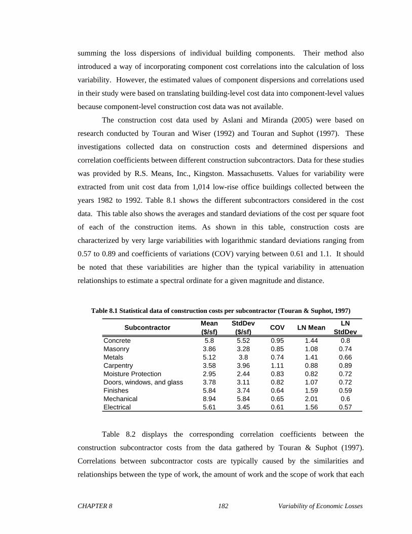
CHAPTER 8 182 Variability of Economic Losses
summing the loss dispersions of individual building components. Their method also
introduced a way of incorporating component cost correlations into the calculation of loss
variability. However, the estimated values of component dispersions and correlations used
in their study were based on translating building-level cost data into component-level values
because component-level construction cost data was not available.
The construction cost data used by Aslani and Miranda (2005) were based on
research conducted by Touran and Wiser (1992) and Touran and Suphot (1997). These
investigations collected data on construction costs and determined dispersions and
correlation coefficients between different construction subcontractors. Data for these studies
was provided by R.S. Means, Inc., Kingston. Massachusetts. Values for variability were
extracted from unit cost data from 1,014 low-rise office buildings collected between the
years 1982 to 1992. Table 8.1 shows the different subcontractors considered in the cost
data. This table also shows the averages and standard deviations of the cost per square foot
of each of the construction items. As shown in this table, construction costs are
characterized by very large variabilities with logarithmic standard deviations ranging from
0.57 to 0.89 and coefficients of variations (COV) varying between 0.61 and 1.1. It should
be noted that these variabilities are higher than the typical variability in attenuation
relationships to estimate a spectral ordinate for a given magnitude and distance.
Table 8.1 Statistical data of construction costs per subcontractor (Touran & Suphot, 1997)
SubcontractorMean ($/sf)
StdDev ($/sf)
COV LN MeanLN
StdDevConcrete 5.8 5.52 0.95 1.44 0.8Masonry 3.86 3.28 0.85 1.08 0.74Metals 5.12 3.8 0.74 1.41 0.66Carpentry 3.58 3.96 1.11 0.88 0.89Moisture Protection 2.95 2.44 0.83 0.82 0.72Doors, windows, and glass 3.78 3.11 0.82 1.07 0.72Finishes 5.84 3.74 0.64 1.59 0.59Mechanical 8.94 5.84 0.65 2.01 0.6Electrical 5.61 3.45 0.61 1.56 0.57
Table 8.2 displays the corresponding correlation coefficients between the
construction subcontractor costs from the data gathered by Touran & Suphot (1997).
Correlations between subcontractor costs are typically caused by the similarities and
relationships between the type of work, the amount of work and the scope of work that each

CHAPTER 8 183 Variability of Economic Losses
subcontractor does. As shown in this table, with a few exceptions, costs from different
subcontractors are typically positively correlated with several of them strongly correlated.
For instance, the costs due to the mechanical and electrical subcontractors are highly
correlated (0.79). Typically the amount and complexity of work that the mechanical
subcontractor does is closely related to the work the electrical subcontractor conducts
because much the building’s mechanical equipment and infrastructure is dependent on the
building’s electrical system.
Table 8.2 Correlation coefficients of construction costs between different subcontractors
Subcontractor Concrete Masonry Metals CarpentryMoisture
Protection
Doors, Windows,
GlassFinishes Mech'l Electrical
Concrete 1.00 0.06 0.11 -0.04 0.19 0.12 0.21 0.38 0.40Masonry 0.06 1.00 -0.01 0.11 0.06 0.14 0.22 0.33 0.30
Metals 0.11 -0.01 1.00 -0.33 0.12 0.39 0.20 0.35 0.33Carpentry -0.04 0.11 -0.33 1.00 0.18 0.03 0.07 -0.02 0.07
Moisture Protection 0.19 0.06 0.12 0.18 1.00 0.16 0.18 0.18 0.15Doors, Windows, Glass 0.12 0.14 0.39 0.03 0.16 1.00 0.25 0.28 0.36
Finishes 0.21 0.22 0.20 0.07 0.18 0.25 1.00 0.42 0.44Mechanical 0.38 0.33 0.35 -0.02 0.18 0.28 0.42 1.00 0.79
Electrical 0.40 0.30 0.33 0.07 0.15 0.36 0.44 0.79 1.00
Unfortunately, the use of building-level cost dispersions and correlations to
approximate values at the component level is difficult to validate. An improved approach is
needed to make use of the cost data provided by Touran & Suphot (1997). The first step of
the approach proposed in this study is establishing a relationship between the cost of each
component to the costs of each subcontractor for the entire building. To accomplish this, the
cost of each component is divided into the contributions of each subcontractor. The cost of
each subcontractor can then be summed to get the total cost for the entire building.
In Chapter 3 of this dissertation, an inventory of building components was
developed to estimate losses for a reinforced concrete moment-frame office building, using
a simplified methodology of building-specific loss estimation. Table 8.3 shows the cost of
each component distributed into each of the subcontractors listed in Touran & Suphot
(1997). The assumed cost distributions were developed with the help of a former cost
estimator, Carlos Sempere, who now works as a design engineer for Forell/Elssesser
Structural Engineers, Inc. These distributions were used to compute loss dispersion for
each subcontractor for the entire building, so the correlations between the costs of different
sub-contractors can be accounted for.

CHAPTER 8 184 Variability of Economic Losses
Table 8.3 Example cost distribution between construction subcontractors of each component in a typical story of an office building
A. SUBSTRUCTUREFoundation 25% 75% 0% 0% 0% 0% 0% 0% 0% 0%
B. SHELLB10 Superstructure
Columns 0% 100% 0% 0% 0% 0% 0% 0% 0% 0%Slab 0% 100% 0% 0% 0% 0% 0% 0% 0% 0%Beam-column joint 0% 100% 0% 0% 0% 0% 0% 0% 0% 0%Slab-column joint 0% 100% 0% 0% 0% 0% 0% 0% 0% 0%
B20 Exterior EnclosureExterior Walls 0% 0% 0% 0% 0% 0% 0% 100% 0% 0%Exterior Windows 0% 0% 0% 0% 0% 0% 100% 0% 0% 0%Exterior Doors 0% 0% 0% 0% 0% 0% 100% 0% 0% 0%
B30 RoofingRoof Coverings 0% 0% 0% 0% 0% 100% 0% 0% 0% 0%Roof Openings 0% 0% 0% 0% 0% 100% 0% 0% 0% 0%
C. INTERIORSPartitions with finishes 0% 0% 0% 40% 0% 0% 0% 60% 0% 0%Interior Doors 0% 0% 0% 0% 0% 0% 100% 0% 0% 0%Fittings 0% 0% 0% 0% 0% 0% 50% 50% 0% 0%Stair Construction 0% 5% 0% 90% 0% 0% 0% 5% 0% 0%Floor Finishes 0% 0% 0% 0% 0% 0% 0% 100% 0% 0%
0% 0% 0% 0% 0% 0% 0% 100% 0% 0%0% 0% 0% 0% 0% 0% 0% 100% 0% 0%
Ceiling Finishes 0% 0% 0% 0% 0% 0% 0% 100% 0% 0%
D. SERVICESD10 Conveying
Elevators & Lifts 0% 0% 0% 0% 0% 0% 0% 0% 100% 0%0% 0% 0% 0% 0% 0% 0% 0% 100% 0%
Escalators & Moving WalksD20 Plumbing
Plumbing Fixtures 0% 0% 0% 0% 0% 0% 0% 0% 100% 0%0% 0% 0% 0% 0% 0% 0% 0% 100% 0%
Domestic Water Distribution 0% 0% 0% 0% 0% 0% 0% 0% 100% 0%Rain Water Drainage 0% 0% 0% 0% 0% 0% 0% 0% 100% 0%
D30 HVACEnergy Supply 0% 0% 0% 0% 0% 0% 0% 0% 100% 0%Heat Generating Systems 0% 0% 0% 0% 0% 0% 0% 0% 100% 0%Cooling Generating Systems 0% 0% 0% 0% 0% 0% 0% 0% 100% 0%Terminal & Package Units 0% 0% 0% 0% 0% 0% 0% 0% 100% 0%
0% 0% 0% 0% 0% 0% 0% 0% 100% 0%Other HVAC Sys. & Equipment 0% 0% 0% 0% 0% 0% 0% 0% 100% 0%
D40 Fire ProtectionSprinklers 0% 0% 0% 0% 0% 0% 0% 0% 100% 0%Standpipes 0% 0% 0% 0% 0% 0% 0% 0% 100% 0%
D50 ElectricalElectrical Service/Distribution 0% 0% 0% 0% 0% 0% 0% 0% 0% 100%Lighting & Branch Wiring 0% 0% 0% 0% 0% 0% 0% 0% 0% 100%Lighting & Branch Wiring 0% 0% 0% 0% 0% 0% 0% 0% 0% 100%Lighting & Branch Wiring 0% 0% 0% 0% 0% 3% 0% 0% 0% 100%Communications & Security 0% 0% 0% 0% 0% 0% 0% 0% 0% 100%Communications & Security 0% 0% 0% 0% 0% 0% 0% 0% 0% 100%Communications & Security 0% 0% 0% 0% 0% 0% 0% 0% 0% 100%Other Electrical Systems 0% 0% 0% 0% 0% 0% 0% 0% 0% 100%
Performance Group CarpentryDoors,
Windows, Glass
FinishesSitework Concrete Masonry Metals Mechanical ElectricalMoisture
Protection
8.3.1.1 Inherent subcontractor cost correlation due to work performed on the same floor/story
In addition to the correlations between subcontractor costs that are obtained from
construction cost data, there is another type of correlation between subcontractor losses that
needs to be accounted for. Monetary losses due to work done by different subcontractors on
drift-sensitive components on the same floor/story will be fully correlated because the
damage on that floor/story will depend on the same EDP. Similarly, economic losses due to
repairs done by different subcontractors on acceleration-sensitive components on the same
floor/story will be fully correlated because the damage on that floor/story will depend on
the same EDP. As a result, when the losses due to each subcontractor are summed for the
entire building, the total losses due to each subcontractor will be correlated because their
losses per floor are fully correlated. That is, a significant amount of work done by different
subcontractors will be correlated because portions of the work are triggered by the same
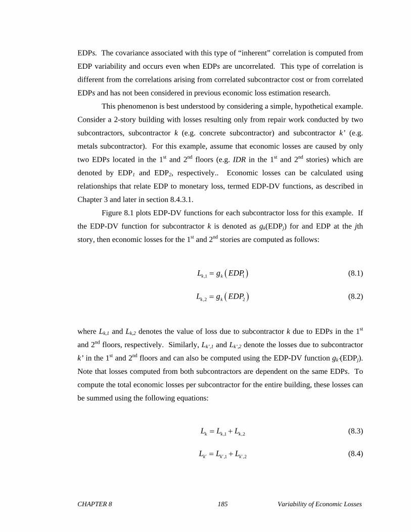
CHAPTER 8 185 Variability of Economic Losses
EDPs. The covariance associated with this type of “inherent” correlation is computed from
EDP variability and occurs even when EDPs are uncorrelated. This type of correlation is
different from the correlations arising from correlated subcontractor cost or from correlated
EDPs and has not been considered in previous economic loss estimation research.
This phenomenon is best understood by considering a simple, hypothetical example.
Consider a 2-story building with losses resulting only from repair work conducted by two
subcontractors, subcontractor k (e.g. concrete subcontractor) and subcontractor k’ (e.g.
metals subcontractor). For this example, assume that economic losses are caused by only
two EDPs located in the 1st and 2nd floors (e.g. IDR in the 1st and 2nd stories) which are
denoted by EDP1 and EDP2, respectively.. Economic losses can be calculated using
relationships that relate EDP to monetary loss, termed EDP-DV functions, as described in
Chapter 3 and later in section 8.4.3.1.
Figure 8.1 plots EDP-DV functions for each subcontractor loss for this example. If
the EDP-DV function for subcontractor k is denoted as gk(EDPj) for and EDP at the jth
story, then economic losses for the 1st and 2nd stories are computed as follows:
,1 1k kL g EDP (8.1)
,2 2k kL g EDP (8.2)
where Lk,1 and Lk,2 denotes the value of loss due to subcontractor k due to EDPs in the 1st
and 2nd floors, respectively. Similarly, Lk’,1 and Lk’,2 denote the losses due to subcontractor
k’ in the 1st and 2nd floors and can also be computed using the EDP-DV function gk’(EDPj).
Note that losses computed from both subcontractors are dependent on the same EDPs. To
compute the total economic losses per subcontractor for the entire building, these losses can
be summed using the following equations:
,1 ,2k k kL L L (8.3)
,1 ,2k k kL L L (8.4)

CHAPTER 8 186 Variability of Economic Losses
where Lk and Lk’ are the total losses for all stories of subcontractor k and subcontractor k’,
respectively. To facilitate the understanding of the source of this additional correlation on
the cost, equations (8.1) and (8.2) can be substituted into (8.3), and the analogous equations
for subcontractor k’ can be substituted into (8.4), to obtain:
1 2k k kL g EDP g EDP (8.5)
1 2k k kL g EDP g EDP (8.6)
These equations demonstrate that because 1kg EDP and 1kg EDP are both dependent
on EDP1 they are highly correlated. Similarly, 2kg EDP and 2kg EDP are also highly
correlated because both are dependent on EDP2. This implies that correlation will also
exists between the losses due to work performed by subcontractor k and subcontractor k’, Lk
and Lk’ even if constructions costs of subcontractors k and k’ are uncorrelated.
Lk,1
Lk,2
EDP2
EDP
E[Lk | EDP]
EDP1
11 22
(a) Subcontractor k
k,1k,1
k,2
Lk,1
Lk,2
EDP2
EDP
E[Lk | EDP]
EDP1
11 22
(a) Subcontractor k
k,1k,1
k,2

CHAPTER 8 187 Variability of Economic Losses
Lk’,1
Lk’,2
EDP2
EDP
E[Lk’ | EDP]
EDP1
11 22
(b) Subcontractor k'
k’,1
k’,1
k’,2
k’,2
Lk’,1
Lk’,2
EDP2
EDP
E[Lk’ | EDP]
EDP1
11 22
(b) Subcontractor k'
k’,1
k’,1
k’,2
k’,2
1. Figure 8.1 Correlation between subcontractor losses due to EDP variance (a) EDP-DV function for subcontractor k (b) EDP-DV function for subcontractor k'
This type of correlation will influence the variability of Lk and Lk’ even when the
EDPs are uncorrelated. EDP1 and EDP2 can be modeled as random variables using
probability distributions as shown in the figure with standard deviations, 1 and 2,
respectively. The EDP-DV functions can be used to propagate the dispersion of the EDPs
to loss dispersions for each subcontractor at each floor using either FOSM or simulation
methods (as will be demonstrated in greater detail later in section 8.4.3.2). For the purposes
of this illustrative example, FOSM can be used to compute the dispersion of the losses due
to EDP variability as follows:
2,1k
1
2
2 2,1 1
1EDP
kk
m
g
EDP
(8.7)
1
2
2 2,2 2
2EDP
kk
m
g
EDP
(8.8)

CHAPTER 8 188 Variability of Economic Losses
where k,1 and k,2 are the resulting standard deviations of the loss of subcontractor k in the
1st and 2nd floors, respectively, and 1
1EDP
k mg EDP and
22
EDPk m
g EDP are the
derivatives of k jg EDP evaluated at the mean values of EDP1 (mEDP1) and EDP2 (mEDP1),
respectively. Likewise, the standard deviations of the loss of subcontractor k’, denoted k’,1
and k’,2 for dispersions at the 1st and 2nd floor respectively, can be found using analogous
expressions using the derivatives of k jg EDP . Assuming that the EDPs at different
stories are uncorrelated, the total dispersion for each subcontractor can be found using the
sum of squares as shown using these equations:
2 2 2,1 ,2k k k (8.9)
2 2 2,1 ,2k k k (8.10)
where k and k’ and are the standard deviations of economic losses for work performed by
subcontractor k and subcontractor k’ in all floors, respectively. To obtain the dispersion of
economic losses of the entire building, the results from equations (8.9) and (8.10) can be
summed together. However, because this inherent correlation between losses due to work
performed by different subcontractors exists, the covariance produced by this correlation
needs to be accounted for as follows:
2 2 2,2BLDG k k k k (8.11)
where BLDG is the standard deviation of economic loss for the entire building and k,k’ is the
covariance between losses due work performed by subcontractor k and subcontractor k’ that
results from this inherent correlation. This covariance can be estimated as follows:
1 1 2 2
2 2, 1 2
1 1 2 2EDP EDP EDP EDP
k k k kk k
m m m m
g g g g
EDP EDP EDP EDP
(8.12)

CHAPTER 8 189 Variability of Economic Losses
Note that equations (8.11) and (8.12) do not involve EDP correlations or construction cost
correlations described in the previous section. This means that this inherent correlation may
affect the overall loss dispersion of the building even if the EDPs and constructions costs
between different subcontractors are uncorrelated. A more generalized version of
computing the variances that account for all these sources of correlation is described in
greater detail in section 8.4.3.
8.3.2 Variability and Correlation in Response Parameters
Capturing the response of a structure to estimate economic loss can be done by
using response parameters such as interstory drift ratio (IDR) and peak floor accelerations
(PFA). Values of peak response parameters can widely vary depending on the ground
motion the structure is subjected to. Figure 8.2 shows the interstory drift in the second story
for a 4-story reinforced concrete moment-resisting frame (ID1009 Haselton & Deierlein,
2007) when subjected to 80 different ground motions scaled to the same intensity level
(measured as spectral acceleration at the fundamental period, Sa(T1) = 0.05g. Note that in
the figures and tables in this chapter will denote this value as Sa for brevity, however, it is
implied that this value is at the fundamental period). The structural analysis was performed
using incremental dynamic analysis (IDA). Record-to-record variability due to frequency
content and other ground motion characteristics introduce this type of dispersion into
predicting structural response and consequently into our estimation of economic loss.
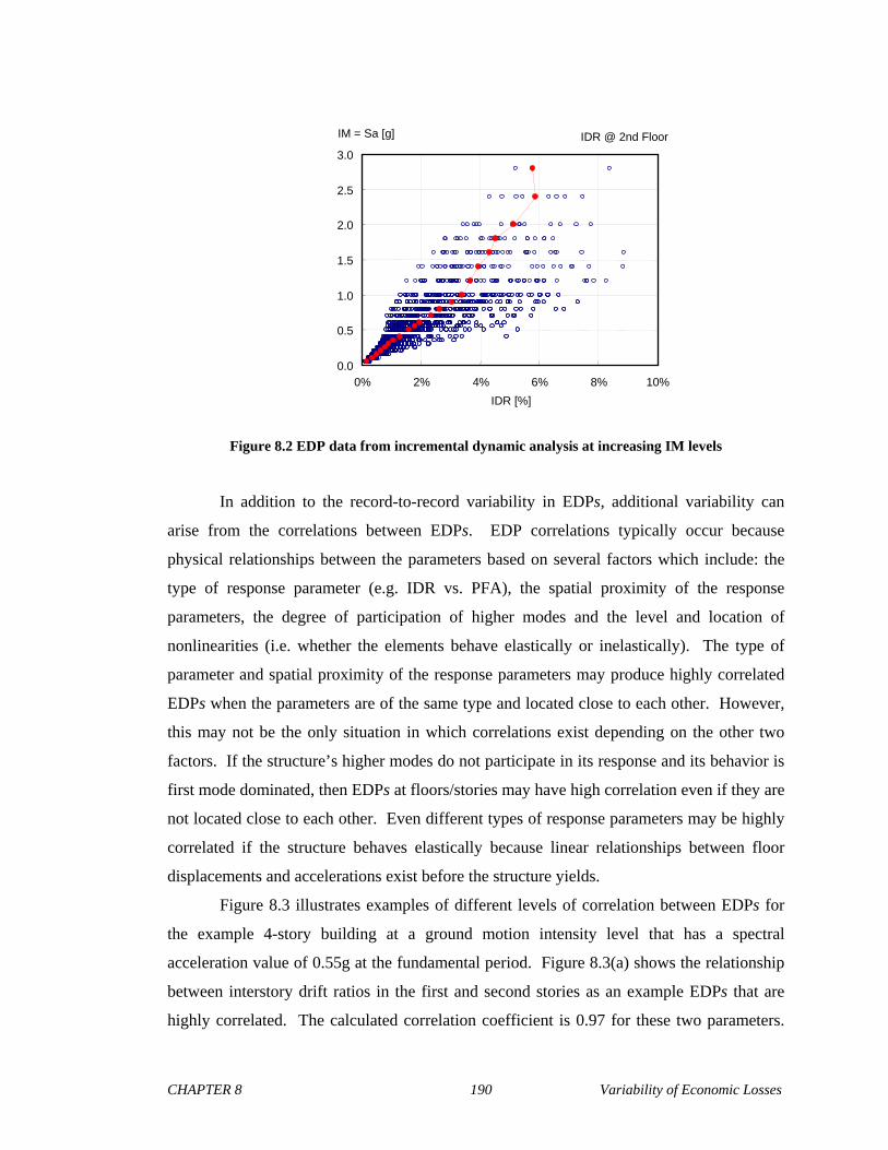
CHAPTER 8 190 Variability of Economic Losses
IDR @ 2nd Floor
0.0
0.5
1.0
1.5
2.0
2.5
3.0
0% 2% 4% 6% 8% 10%
IDR [%]
IM = Sa [g] IDR @ 2nd Floor
0.0
0.5
1.0
1.5
2.0
2.5
3.0
0% 2% 4% 6% 8% 10%
IDR [%]
IM = Sa [g]
Figure 8.2 EDP data from incremental dynamic analysis at increasing IM levels
In addition to the record-to-record variability in EDPs, additional variability can
arise from the correlations between EDPs. EDP correlations typically occur because
physical relationships between the parameters based on several factors which include: the
type of response parameter (e.g. IDR vs. PFA), the spatial proximity of the response
parameters, the degree of participation of higher modes and the level and location of
nonlinearities (i.e. whether the elements behave elastically or inelastically). The type of
parameter and spatial proximity of the response parameters may produce highly correlated
EDPs when the parameters are of the same type and located close to each other. However,
this may not be the only situation in which correlations exist depending on the other two
factors. If the structure’s higher modes do not participate in its response and its behavior is
first mode dominated, then EDPs at floors/stories may have high correlation even if they are
not located close to each other. Even different types of response parameters may be highly
correlated if the structure behaves elastically because linear relationships between floor
displacements and accelerations exist before the structure yields.
Figure 8.3 illustrates examples of different levels of correlation between EDPs for
the example 4-story building at a ground motion intensity level that has a spectral
acceleration value of 0.55g at the fundamental period. Figure 8.3(a) shows the relationship
between interstory drift ratios in the first and second stories as an example EDPs that are
highly correlated. The calculated correlation coefficient is 0.97 for these two parameters.
CHAPTER 8 191 Variability of Economic Losses
An example of partial correlation is plotted in Figure 8.3(b). The relationship between PFA
in the second floor and IDR in the second story has a correlation coefficient of 0.58.
Finally, EDPs can also be uncorrelated as shown in Figure 8.3(c); this figure shows the
relationship between IDR in the second floor and PFA in the fourth floor, which has a
correlation coefficient of 0.041.
0.00
0.02
0.04
0.06
0 0.02 0.04 0.06 0.08
IDR @ 1st Story
IDR @ 2nd Story
= 0.97
(a) Sa = 0.55g
0.0
0.5
1.0
1.5
0 0.01 0.02 0.03
IDR @ 4th Story
PFA @ 4th Floor [g]
= 0.58
(b) Sa = 0.55g
0.0
0.5
1.0
1.5
0 0.02 0.04 0.06 0.08
IDR @ 1st Story
PFA @ 4th Floor [g]
= 0.041
(c) Sa = 0.55g
Figure 8.3 Example of EDP relationships with different levels of correlation
Correlations between response parameters can also vary as the intensity level of the
ground motions is increased. Figure 8.4 shows scatter plots between different EDPs at two
different levels of ground motion intensity. It can be observed from these plots that
parameters that are highly correlated at lower intensity levels can either remain highly
correlated, or decrease their level of correlation at higher levels of intensity (Figure 8.4 (a)
to (d)). On the other hand, parameters that are initially poorly correlated, can increase their
level of correlation as the earthquake intensity is increased (Figure 8.4 (e) to (f)). To better
illustrate this, Figure 8.5 plots correlations coefficients for a range of seismic intensities
(measured in spectral acceleration at the fundamental period, Sa(T1)). The figure shows the
same three trends of variation in correlation coefficients in Figure 8.4. Most changes in
correlation occur because of the change from elastic to inelastic behavior when damage
occurs to the structure. For instance, IDR in the fourth story and PFA in the fifth floor are
highly correlated at lower ground motion intensities because they are close in proximity to
each other, the structure is likely first-mode dominated (low-rises structure) and because
linear relationships exist between displacements and accelerations before the structure
yields. However, the EDP correlation decreases at higher seismic intensities because at

CHAPTER 8 192 Variability of Economic Losses
these ground motions the structure has yielded and lateral deformation concentrates in
members where plastic hinges have developed. Once these hinges form, the linear
relationships between displacements and accelerations do not necessarily hold.
0.000
0.002
0.004
0.006
0.008
0.010
0 0.002 0.004 0.006 0.008
IDR @ 1st Story
IDR @ 2nd Story
= 0.97
(a) Sa = 0.25g
0.00
0.02
0.04
0.06
0.08
0.10
0 0.02 0.04 0.06 0.08 0.1
IDR @ 1st Story
IDR @ 2nd Story
= 0.95
(b) Sa = 1.6g
0.0
0.1
0.2
0.3
0.4
0.5
0 0.001 0.002 0.003 0.004
IDR @ 4th Story
PFA @ 5th Floor [g]
= 0.87
(c) Sa = 0.25g
0.0
0.5
1.0
1.5
2.0
2.5
0 0.02 0.04 0.06 0.08 0.1
IDR @ 4th Story
PFA @ 5th Floor [g]
= 0.18
(d) Sa = 1.6g
0.00000
0.00005
0.00010
0.00015
0.00020
0.00025
0 0.001 0.002 0.003 0.004
IDR @ 4th Story
RIDR @ 4th Story
= 0.22
(e) Sa = 0.25g
0.00
0.02
0.04
0.06
0.08
0.10
0 0.02 0.04 0.06 0.08 0.1
IDR @ 4th Story
RIDR @ 4th Story
= 0.79
(f) Sa = 1.6g
Figure 8.4 Correlation trends at low and high seismic intensity levels

CHAPTER 8 193 Variability of Economic Losses
-1.00
-0.50
0.00
0.50
1.00
0.0 0.5 1.0 1.5 2.0
IM = Sa [g]
IDR2 & IDR1
-1.00
-0.50
0.00
0.50
1.00
0.0 0.5 1.0 1.5 2.0
IM = Sa [g]
PFA5 & IDR4
-1.00
-0.50
0.00
0.50
1.00
0.0 0.5 1.0 1.5 2.0
IM = Sa [g]
RIDR4 & IDR4
(a) (b) (c)
-1.00
-0.50
0.00
0.50
1.00
0.0 0.5 1.0 1.5 2.0
IM = Sa [g]
IDR2 & IDR1
-1.00
-0.50
0.00
0.50
1.00
0.0 0.5 1.0 1.5 2.0
IM = Sa [g]
PFA5 & IDR4
-1.00
-0.50
0.00
0.50
1.00
0.0 0.5 1.0 1.5 2.0
IM = Sa [g]
RIDR4 & IDR4
(a) (b) (c)
Figure 8.5 Variation of EDP correlation with intensity level
8.3.2.1 EDP correlation coefficient estimates
Although structural analysis data is readily available to determine EDP correlations,
it must be recognized that the values calculated are only estimations of the true correlations.
Obtaining the true correlations requires subjecting the considered building to all ground
motions possible at the structure’s site. This is impossible because all possible ground
motions are not known. Instead, the building is subjected to a sample of ground motions
from which only approximate what the EDP correlations can be obtained. The accuracy of
these approximate correlations depends on the number of ground motions being sampled in
the structural analysis. Unfortunately, using a large number of ground motions can be
computational expensive and time consuming. The issue of how many ground motions
should be considered has been much debated. However, previous work has been primarily
aimed at determining the number of ground motions required to obtain estimates of median
response/loss (e.g. expected loss, probability of collapse…etc.). There has been little work
on how many ground motions are necessary to obtain good estimates of EDP correlation
coefficients.
Since the actual distribution of correlation coefficients is unknown, an approximate
distribution can be obtained by using bootstrap sampling. Bootstrap sampling is a
resampling method (with replacement) that uses data collected for a single sample to
simulate results for multiple samples, without repeating the procedure required to obtain the
original data (Efron 1979, 1982). It is often used in studies where data collection is limited,
such as in medical studies. Bootstrap sampling will used here to demonstrate how this
procedure can be used to obtain reliable estimates of response parameter correlation

CHAPTER 8 194 Variability of Economic Losses
coefficients. Further, it will also be shown how bootstrap sampling can be used to evaluate
how reliable the correlation coefficient estimates are depending on the sample size of the
ground motions being considered.
The same 4-story concrete moment frame building taken from Haselton & Deierlein
(2007) previously discussed in the preceding paragraphs can be used to illustrate the use of
the bootstrap method to predict EDP correlations coefficients. Haselton & Deierlein used a
sample of 80 ground motions to obtain EDPs at different values of ground motion intensity.
For a given intensity level, only one set of EDP correlations coefficients can computed from
this sample. However, there is no way of knowing how variable the estimates of the
correlation coefficients are. When using bootstrapping, a new sample of 80 ground motions
are randomly extracted out of the existing 80 ground motions, where each ground motion
can be selected at most 80 times (i.e. a ground motion can be considered more than once
during resampling). The EDPs computed from the new sample of ground motions can be
used to generate another realization of correlation coefficients. Repeating this process for a
large number of realizations, probability distributions of the correlation coefficients can be
estimated by obtaining the mean and standard deviation of each coefficient.
Table 8.4 shows the mean correlation coefficient matrix for the Haselton &
Deierlein (2007) 4-story concrete moment frame building using 1000 bootstrap realizations.
Correlations were computed for IDRs, PFAs and residual interstory drifts (RIDRs). Also
documented are the standard deviations of these coefficients in Table 8.5. In these tables
the type of EDP is listed followed by the location where it is located along the height of the
building (e.g. IDR1 corresponds to IDR in the 1st story and PFA2 corresponds to PFA in the
2nd floor).
Table 8.4 Average of EDP correlation coefficients from 1000 realizations
IDR1 IDR2 IDR3 IDR4 RIDR1 RIDR2 RIDR3 RIDR4 PGA PFA2 PFA3 PFA4 PFA5IDR1: 1.00 0.97 0.55 0.05 0.95 0.93 0.68 0.16 0.12 0.06 0.01 0.04 0.03IDR2: 0.97 1.00 0.70 0.18 0.93 0.94 0.79 0.30 0.16 0.09 0.05 0.08 0.07IDR3: 0.55 0.70 1.00 0.69 0.54 0.63 0.89 0.73 0.33 0.28 0.30 0.34 0.35IDR4: 0.05 0.18 0.69 1.00 0.07 0.14 0.47 0.86 0.56 0.55 0.58 0.58 0.60
RIDR1: 0.95 0.93 0.54 0.07 1.00 0.99 0.74 0.19 0.12 0.06 0.01 0.03 0.01RIDR2: 0.93 0.94 0.63 0.14 0.99 1.00 0.82 0.28 0.15 0.09 0.05 0.06 0.05RIDR3: 0.68 0.79 0.89 0.47 0.74 0.82 1.00 0.63 0.20 0.16 0.16 0.19 0.19RIDR4: 0.16 0.30 0.73 0.86 0.19 0.28 0.63 1.00 0.36 0.38 0.40 0.40 0.41
PGA [g]: 0.12 0.16 0.33 0.56 0.12 0.15 0.20 0.36 1.00 0.89 0.84 0.79 0.78PFA2 [g]: 0.06 0.09 0.28 0.55 0.06 0.09 0.16 0.38 0.89 1.00 0.93 0.84 0.85PFA3 [g]: 0.01 0.05 0.30 0.58 0.01 0.05 0.16 0.40 0.84 0.93 1.00 0.87 0.88PFA4 [g]: 0.04 0.08 0.34 0.58 0.03 0.06 0.19 0.40 0.79 0.84 0.87 1.00 0.85PFA5 [g]: 0.03 0.07 0.35 0.60 0.01 0.05 0.19 0.41 0.78 0.85 0.88 0.85 1.00
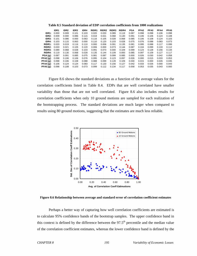
CHAPTER 8 195 Variability of Economic Losses
Table 8.5 Standard deviation of EDP correlation coefficients from 1000 realizations
IDR1 IDR2 IDR3 IDR4 RIDR1 RIDR2 RIDR3 RIDR4 PGA PFA2 PFA3 PFA4 PFA5IDR1: 0.000 0.009 0.101 0.103 0.020 0.033 0.089 0.119 0.087 0.098 0.098 0.106 0.098IDR2: 0.009 0.000 0.086 0.115 0.019 0.021 0.068 0.130 0.091 0.106 0.106 0.124 0.108IDR3: 0.101 0.086 0.000 0.063 0.116 0.105 0.028 0.068 0.085 0.106 0.108 0.124 0.103IDR4: 0.103 0.115 0.063 0.000 0.110 0.120 0.103 0.028 0.075 0.076 0.088 0.083 0.073
RIDR1: 0.020 0.019 0.116 0.110 0.000 0.006 0.091 0.135 0.081 0.095 0.088 0.117 0.099RIDR2: 0.033 0.021 0.105 0.120 0.006 0.000 0.073 0.144 0.087 0.104 0.099 0.133 0.112RIDR3: 0.089 0.068 0.028 0.103 0.091 0.073 0.000 0.109 0.099 0.123 0.128 0.156 0.134RIDR4: 0.119 0.130 0.068 0.028 0.135 0.144 0.109 0.000 0.085 0.097 0.109 0.127 0.117
PGA [g]: 0.087 0.091 0.085 0.075 0.081 0.087 0.099 0.085 0.000 0.026 0.030 0.042 0.058PFA2 [g]: 0.098 0.106 0.106 0.076 0.095 0.104 0.123 0.097 0.026 0.000 0.015 0.033 0.053PFA3 [g]: 0.098 0.106 0.108 0.088 0.088 0.099 0.128 0.109 0.030 0.015 0.000 0.026 0.035PFA4 [g]: 0.106 0.124 0.124 0.083 0.117 0.133 0.156 0.127 0.042 0.033 0.026 0.000 0.043PFA5 [g]: 0.098 0.108 0.103 0.073 0.099 0.112 0.134 0.117 0.058 0.053 0.035 0.043 0.000
Figure 8.6 shows the standard deviations as a function of the average values for the
correlation coefficients listed in Table 8.4. EDPs that are well correlated have smaller
variability than those that are not well correlated. Figure 8.6 also includes results for
correlation coefficients when only 10 ground motions are sampled for each realization of
the bootstrapping process. The standard deviations are much larger when compared to
results using 80 ground motions, suggesting that the estimates are much less reliable.
0.00
0.10
0.20
0.30
0.40
0.50
0.00 0.20 0.40 0.60 0.80 1.00
Avg. of Correlation Coeff Estimations
Std
. D
ev.o
f C
orr
elat
ion
Co
eff
Est
imat
ion
s
80 Ground Motions
10 Ground Motions
Figure 8.6 Relationship between average and standard error of correlation coefficient estimates
Perhaps a better way of capturing how well correlation coefficients are estimated is
to calculate 95% confidence bands of the bootstrap samples. The upper confidence band in
this context is defined by the difference between the 97.5th percentile and the median value
of the correlation coefficient estimates, whereas the lower confidence band is defined by the
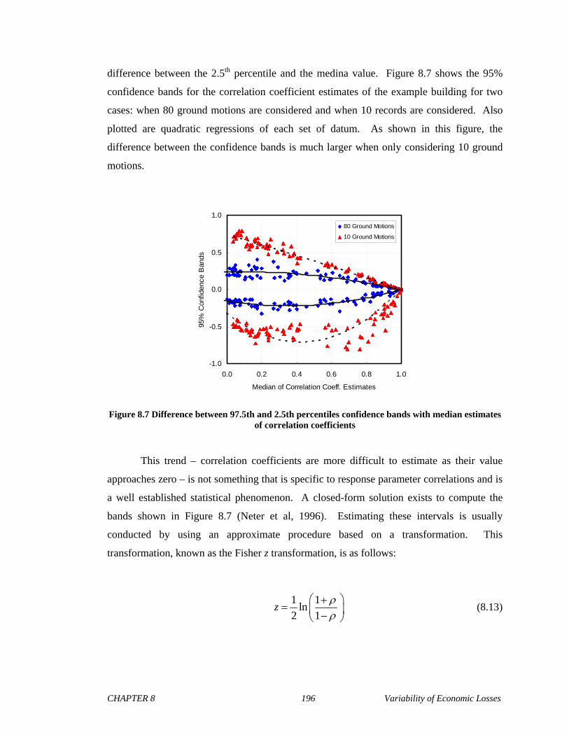
CHAPTER 8 196 Variability of Economic Losses
difference between the 2.5th percentile and the medina value. Figure 8.7 shows the 95%
confidence bands for the correlation coefficient estimates of the example building for two
cases: when 80 ground motions are considered and when 10 records are considered. Also
plotted are quadratic regressions of each set of datum. As shown in this figure, the
difference between the confidence bands is much larger when only considering 10 ground
motions.
-1.0
-0.5
0.0
0.5
1.0
0.0 0.2 0.4 0.6 0.8 1.0
Median of Correlation Coeff. Estimates
95%
Con
fiden
ce B
ands
80 Ground Motions
10 Ground Motions
Figure 8.7 Difference between 97.5th and 2.5th percentiles confidence bands with median estimates of correlation coefficients
This trend – correlation coefficients are more difficult to estimate as their value
approaches zero – is not something that is specific to response parameter correlations and is
a well established statistical phenomenon. A closed-form solution exists to compute the
bands shown in Figure 8.7 (Neter et al, 1996). Estimating these intervals is usually
conducted by using an approximate procedure based on a transformation. This
transformation, known as the Fisher z transformation, is as follows:
1 1
ln2 1
z (8.13)

CHAPTER 8 197 Variability of Economic Losses
where is the value of correlation coefficient for which confidence bands are being
computed. The distribution of z is assumed to be approximately normal such that its
variance is equal to:
2 1
3z N
(8.14)
where N is the number of ground motions being considered. Correspondingly, if z is
assumed normal, the approximate 95% confidence limits for the expected value of z is:
1.96 zz (8.15)
where 1.96 is the value of the 1 2 100 percentile of the standard normal distribution
for confidence value of 95% ( = 5). The 95% confidence limits for can then be
computed by transforming the limits obtained from equation (8.15) back in terms of using
the inverse solution of equation (8.13). Figure 8.8(b) compares the results from this
procedure to the bands obtained from the example building’s EDP data for N = 10 and 80.
The figure shows that there is fairly good agreement between the EDP data generated from
the bootstrap sampling and the analytical procedure. Figure 8.8(a) uses the analytical
procedure to approximate the 95% confidence bands for N = 10, 20, 40 and 80 ground
motions. As the number of ground motions considered are decreased, the difference
between confidence bands and median increases. This procedure can be used to help
engineers decide how many ground motions to use during structural analysis based on how
well analysts would like to approximate EDP correlation coefficients.

CHAPTER 8 198 Variability of Economic Losses
-1.0
-0.5
0.0
0.5
1.0
0.0 0.2 0.4 0.6 0.8 1.0
Median of Correlation Coeff. Estimates
95%
Con
fiden
ce B
ands
N = 80: AnalyticalN = 10: AnalyticalN = 10: DataN = 80: Data
-1.0
-0.5
0.0
0.5
1.0
0.0 0.2 0.4 0.6 0.8 1.0
Median of Correlation Coeff. Estimates
95%
Con
fiden
ce B
ands
N = 10N = 20N = 40N = 80
(a) (b)
-1.0
-0.5
0.0
0.5
1.0
0.0 0.2 0.4 0.6 0.8 1.0
Median of Correlation Coeff. Estimates
95%
Con
fiden
ce B
ands
N = 80: AnalyticalN = 10: AnalyticalN = 10: DataN = 80: Data
-1.0
-0.5
0.0
0.5
1.0
0.0 0.2 0.4 0.6 0.8 1.0
Median of Correlation Coeff. Estimates
95%
Con
fiden
ce B
ands
N = 10N = 20N = 40N = 80
(a) (b)
Figure 8.8 Confidence bands using closed form solution for different number of ground motions (a) bands for N = 10, 20, 40 and 80 (b) comparison with data from example building.
The confidence bands in Figure 8.8 illustrate that the number of ground motions
considered can have a large effect on the EDP correlation coefficients estimated and,
consequently, can have a large effect on the value of economic loss dispersion computed.
For instance, the mean correlation coefficient between the 3rd story IDR and the 3rd floor
PFA is equal to 0.30 for the example building (given that the spectral acceleration at the
fundamental period equal to 0.55g’s) as shown in Table 8.4. According to the results in
Figure 8.8(a), the estimated value of this coefficient could vary between approximately -
0.40 and 0.75 if only 10 ground motions are considered. This means that if only 10 ground
motions are considered, the correlation between these two EDPs can be estimated to be
either negatively correlated or strongly positively correlated. This will yield opposite
effects on the value of the overall economic loss dispersion, resulting in a poor estimate of
the loss variability.
8.3.3 Variability and Correlations in Damage Estimation
Damage to building components due to seismic ground motions is typically
conducted by defining discrete damage states, DS, for each component i. The probability
of experiencing or exceeding each damage state is quantified by defining cumulative

CHAPTER 8 199 Variability of Economic Losses
probability distributions that are based on the level of EDP that the component is subjected
to. These probabilistic relationships between EDP and DS are termed fragility functions.
The variability in damage estimation is quantified by the dispersion of these fragility
functions. These functions can be obtained from experimental data gathered from
laboratory experiments conducted on building components (Porter et al. 2007), from
empirical data observed from earthquake damage experienced in previous seismic events
(Chapter 5) or from using analytical models.
The correlations between building component damage states are difficult to quantify
because it requires knowing the joint probability distribution of components i and i’
conditioned on EDPj and EDPj’ respectively (Aslani and Miranda, 2005). Unfortunately,
data to estimate these joint probably distributions are unavailable and difficult to obtain. In
the absence of data, simplifying assumptions need to be used to account for correlations
between building component damage states. For the purposes of this study, the following is
assumed:
For a given EDP, the levels of damage in the same type of components
located in the same story are fully correlated.
For a given EDP, the damage levels of different types of components have
no correlation.
The assumption that the damage levels are fully correlated for the same type of components
located in the same story is based on the notion that the same types of components are
typically constructed by the same subcontractor. If this is true, the quality of construction
will be the same for these types of components and will most likely experience the same
damage when subjected to the same level of EDP. Conversely, assuming that the levels of
damage are not correlated between different building components is based on the notion
that the quality of construction of one component is not related to another. This is primarily
based on the fact that different sub-contractors tend to operate fairly independently of one
another. The vulnerability of one type of component based on the quality of its construction
is most likely not related to the vulnerability of a different type of component because it
was constructed by a different subcontractor. It may be argued that the quality of
construction between sub-contractors may be related because they are chosen by a common
general contractor; however, there are many factors that go into selecting sub-contractors,
such that any correlation is likely to be weak.
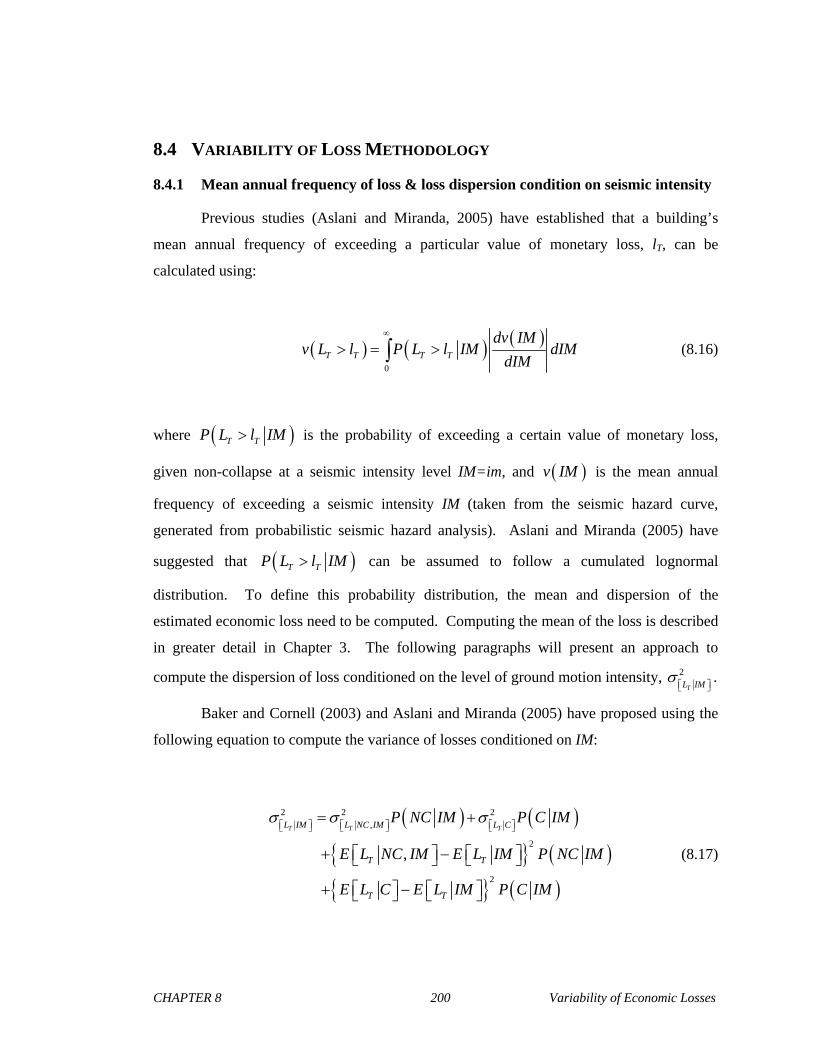
CHAPTER 8 200 Variability of Economic Losses
8.4 VARIABILITY OF LOSS METHODOLOGY
8.4.1 Mean annual frequency of loss & loss dispersion condition on seismic intensity
Previous studies (Aslani and Miranda, 2005) have established that a building’s
mean annual frequency of exceeding a particular value of monetary loss, lT, can be
calculated using:
0
T T T T
dv IMv L l P L l IM dIM
dIM
(8.16)
where T TP L l IM is the probability of exceeding a certain value of monetary loss,
given non-collapse at a seismic intensity level IM=im, and v IM is the mean annual
frequency of exceeding a seismic intensity IM (taken from the seismic hazard curve,
generated from probabilistic seismic hazard analysis). Aslani and Miranda (2005) have
suggested that T TP L l IM can be assumed to follow a cumulated lognormal
distribution. To define this probability distribution, the mean and dispersion of the
estimated economic loss need to be computed. Computing the mean of the loss is described
in greater detail in Chapter 3. The following paragraphs will present an approach to
compute the dispersion of loss conditioned on the level of ground motion intensity, 2 TL IM.
Baker and Cornell (2003) and Aslani and Miranda (2005) have proposed using the
following equation to compute the variance of losses conditioned on IM:
2 2 2,
2
2
,
T T TL IM L NC IM L C
T T
T T
P NC IM P C IM
E L NC IM E L IM P NC IM
E L C E L IM P C IM
(8.17)

CHAPTER 8 201 Variability of Economic Losses
where P NC IM and P C IM are the probabilities of non-collapse and collapse
conditioned on IM, respectively (note that these probabilities are complimentary such that
P NC IM = 1 P C IM . The expected loss conditioned the building not collapsing is
denoted by ,TE L NC IM , the expected loss given that the building collapsed is denoted
by TE L C (taken to be the mean replacement value of the building) and the expected
loss conditioned on the level of ground motion intensity is denoted by TE L IM . The
variance of loss conditioned on collapse and the variance of loss conditioned on non-
collapse are represented by 2
TL C
and 2,
TL NC IM, respectively.
8.4.2 Dispersion of loss conditioned on collapse
The variance of loss conditioned on collapse, 2 TL C, can be computed from
construction cost data similar to those shown in Table 8.2. The expected loss conditioned
on collapse, TE L C , is equal to the replacement value of the building because it is
defined as the cost of constructing a new structure to replace the one that has collapsed
(including the costs for removing the collapsed building). The dispersion associated with
this loss is assumed to be similar to the variability of the cost of constructing a new building
of the same occupancy that can be obtained from construction cost data.
The variance of economic loss conditioned on collapse, 2 TL C, can be obtained
form the standard deviations of the loss conditioned on collapse due to each subcontractor
k, kL C, as follows:
2,
1 1
2,
1 1 1
T k k
k k k
l l
k kL C L C L Ck k
l l l
k kL C L C L Ck k k
k k
(8.18)

CHAPTER 8 202 Variability of Economic Losses
where k,k’ are the cost correlation coefficients that can be obtained from construction cost
data. Note that the equation in (8.18) represents the sum of the covariance matrix for the
economic loss conditioned on collapse. The first line of equation (8.18) can be expanded to
separate the variance (the diagonal terms in the covariance matrix) and covariance (the off-
diagonal terms) terms of the covariance matrix as shown on the second line. The standard
deviation of the loss conditioned on collapse due to each subcontractor k, kL C, is
computed using:
k
k kL CE L C (8.19)
where k is the coefficient of variation of the construction costs for the kth subcontractor
and kE L C is expected economic loss conditioned on collapse for subcontractor k. k
is extracted from construction cost data and kE L C can be found computed from the
building’s replacement value with the following equation:
k k TE L C b E L C (8.20)
where b’k is the normalized proportion of the building replacement cost that is due to the kth
subcontractor. This value can also be determined from construction cost data by dividing
the mean cost of each subcontractor by the total mean cost of the entire building.
8.4.3 Dispersion of loss conditioned on non-collapse
Computing the variance of loss conditioned on non-collapse, 2,
TL NC IM, is more
complicated. Not only does estimating this type of loss dispersion involve the variability of
construction costs, it must account for variabilities from structural response and fragility
functions. The variability due to fragility functions is accounted for indirectly by collapsing

CHAPTER 8 203 Variability of Economic Losses
out the estimation of damage to create functions that relate economic loss and EDPs directly
(EDP-DV functions). These functions, which group building components by subcontractor
and EDP, can be used to propagate the variability and correlations of the building’s
structural response parameters. The variances can be summed for the entire building for
each subcontractor loss. The variability and correlations due to construction costs obtained
from building-level cost data can then be incorporated by adding them to the variances per
subcontractor computed thus far. The variance of each subcontractor can then be summed
together to obtain the dispersion of the economic loss conditioned on non-collapse for the
entire building at a given level of ground motion intensity.
Two implementations of this part of the methodology were developed. The first
implementation, presented in this section, is an approximate analytical approach that relies
on FOSM to compute dispersions. The second implementation, presented in section 8.4.4,
follows the same basic principles as the first but uses Monte Carlo simulation to obtain
dispersion results. Both implementations have advantages and disadvantages. The
analytical approach is not as computationally-intensive but the results are approximate and
may yield poor results depending on the type of building being considered. The approach
using simulation propagates variability accurately but can be computationally expensive
and may take longer to compute.
The nomenclature for the variables presented in the following equations can become
lengthy and confusing if carried out thoroughly and explicitly. Therefore, to simplify
presentation of this approach, it will be implied that from this point forward, all the
variables contained in this section will be conditioned on the building not collapsing, NC,
whether it is explicitly expressed or not. For example, when the expected loss conditioned
on EDP is expressed as E L EDP , it is implied that this value is also conditioned on non-
collapse as well (i.e. it is implied that the expected loss is conditioned on EDP and on the
building not collapsing as if it were expressed using , E L NC EDP ).
8.4.3.1 Collapse out damage estimation and group by subcontractor cost
Estimating damage is collapsed out because the damage states for each component
are discrete random variables. The next step in this approach will involve using FOSM
methods to propagate response parameter dispersions. Using FOSM methods can become
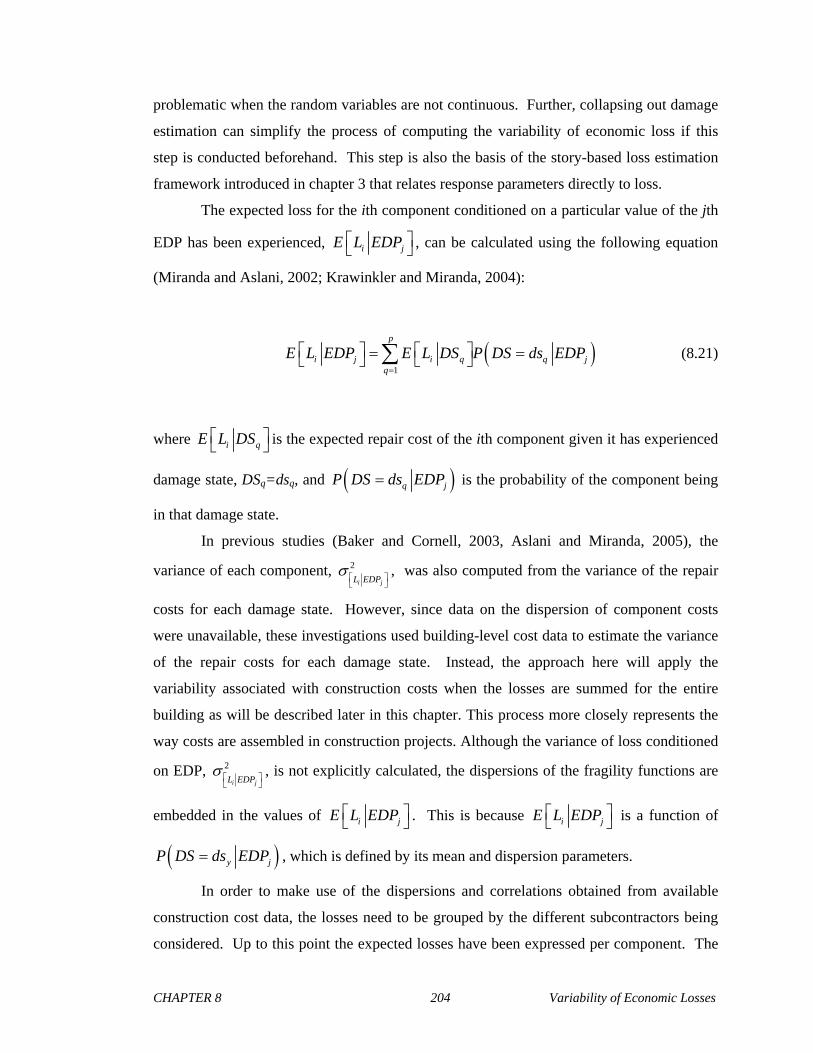
CHAPTER 8 204 Variability of Economic Losses
problematic when the random variables are not continuous. Further, collapsing out damage
estimation can simplify the process of computing the variability of economic loss if this
step is conducted beforehand. This step is also the basis of the story-based loss estimation
framework introduced in chapter 3 that relates response parameters directly to loss.
The expected loss for the ith component conditioned on a particular value of the jth
EDP has been experienced, i jE L EDP , can be calculated using the following equation
(Miranda and Aslani, 2002; Krawinkler and Miranda, 2004):
1
p
i j i q q jq
E L EDP E L DS P DS ds EDP (8.21)
where i qE L DS is the expected repair cost of the ith component given it has experienced
damage state, DSq=dsq, and q jP DS ds EDP is the probability of the component being
in that damage state.
In previous studies (Baker and Cornell, 2003, Aslani and Miranda, 2005), the
variance of each component, 2 i jL EDP
, was also computed from the variance of the repair
costs for each damage state. However, since data on the dispersion of component costs
were unavailable, these investigations used building-level cost data to estimate the variance
of the repair costs for each damage state. Instead, the approach here will apply the
variability associated with construction costs when the losses are summed for the entire
building as will be described later in this chapter. This process more closely represents the
way costs are assembled in construction projects. Although the variance of loss conditioned
on EDP, 2 i jL EDP
, is not explicitly calculated, the dispersions of the fragility functions are
embedded in the values of i jE L EDP . This is because i jE L EDP is a function of
y jP DS ds EDP , which is defined by its mean and dispersion parameters.
In order to make use of the dispersions and correlations obtained from available
construction cost data, the losses need to be grouped by the different subcontractors being
considered. Up to this point the expected losses have been expressed per component. The

CHAPTER 8 205 Variability of Economic Losses
value of each component must be divided in proportion to how much the cost of each
subcontractor contributes to the total value of the repair costs, such that:
, k i j k i jE L EDP b E L EDP (8.22)
where bk is the fraction of the component’s replacement value that is attributed to
subcontractor k. In this study, bk is assumed to be deterministic. Although bk may be
considered a random variable, the relative size of dispersion is deemed to be much smaller
compared to the other sources variability considered in this methodology.
In order to limit the amount of computation required to propagate the variance of
loss given EDP to loss for a given intensity level, IM=im, it is convenient to group
components’ expected values and dispersion by the number of EDPs being considered. The
number of EDPs, m, is a function of the number of stories and the types of EDPs
considered. In this chapter, only two types of EDPs, peak interstory drift (IDR) and peak
floor acceleration (PFA), are considered for each story (the total number EDPs is equal to 2
x the number of stories) for the purposes of computing economic loss dispersion (RIDR is
used as an EDP that is used to estimate the probability of building demolition conditioned
on non-collapse in Chapter 9). Expected values of losses ( , k j jE L EDP ) for the jth EDP
can be summed using the following equation:
, ,1
n
k j j k i ji
E L EDP E L EDP (8.23)
where n is the number of components whose damage depends on the same EDP. This
procedure is the same the one used to formulate the EDP-DV functions described Chapter 3
except that these functions in addition to being grouped by type of EDP, these functions are
also grouped by subcontractor cost using the assumed distributions in Table 8.3. Figure 8.9
and Figure 8.10 shows the subcontract floor used to calculate the dispersions for the
example 4-story reinforced concrete moment-resisting frame building. The expected
economic losses shown in these figures are normalized by the entire value of the story.
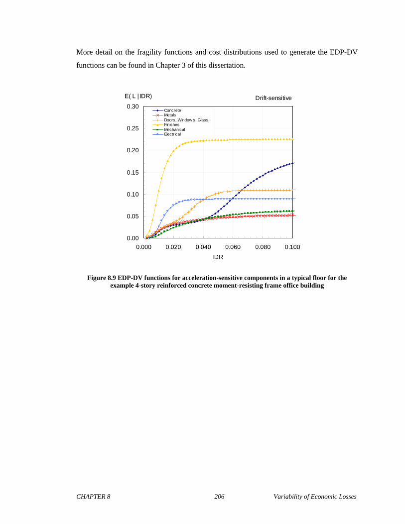
CHAPTER 8 206 Variability of Economic Losses
More detail on the fragility functions and cost distributions used to generate the EDP-DV
functions can be found in Chapter 3 of this dissertation.
Drift-sensitive
0.00
0.05
0.10
0.15
0.20
0.25
0.30
0.000 0.020 0.040 0.060 0.080 0.100
IDR
E( L | IDR)
ConcreteMetalsDoors, Window s, GlassFinishesMechanicalElectrical
Figure 8.9 EDP-DV functions for acceleration-sensitive components in a typical floor for the example 4-story reinforced concrete moment-resisting frame office building

CHAPTER 8 207 Variability of Economic Losses
Acceleration-sensitive
0.00
0.05
0.10
0.15
0.20
0.25
0.30
0.0 1.0 2.0 3.0 4.0 5.0
PFA [g]
E( L | PFA )
Finishes
Mechanical
Electrical
Figure 8.10 EDP-DV functions for drift-sensitive components in a typical floor for the example 4-story reinforced concrete moment-resisting frame office building
8.4.3.2 Propagate variance from response parameters
The subcontractor EDP-DV functions shown in Figure 8.9 and Figure 8.10 can be
combined with the variability of EDPs conditioned on a given intensity level, IM=im, to
compute the dispersion of economic loss as a function of ground motion intensity. The
variability of EDPs for a given ground motion intensity level can be computed from
structural analysis. The EDP-DV functions, which express loss as function of EDP, can
then be used to translate the structural response dispersion into the variability of economic
loss due to the variability of EDP.
It has been suggested by previous investigators to use FOSM approximations to
accomplish this step in variability propagation (Benjamin and Cornell 1970, Ang and Tang
1984, Baker and Cornell 2008). Using the FOSM approach, the economic loss due to work
performed by subcontractor k to repair damage caused by EDP j conditioned on ground
motion intensity, ,k jL IM , can be calculated using a first-order Taylor expansion of the
economic loss due to work performed by subcontractor k to repair damage caused by EDP j,
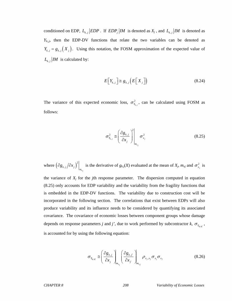
CHAPTER 8 208 Variability of Economic Losses
conditioned on EDP, ,k jL EDP . If jEDP IM is denoted as Xj , and ,k jL IM is denoted as
Yk,,j, then the EDP-DV functions that relate the two variables can be denoted as
, ,k j k j jY g X . Using this notation, the FOSM approximation of the expected value of
,k jL IM is calculated by:
, , k j k j jE Y g E X (8.24)
The variance of this expected economic loss, ,
2
k jY , can be calculated using FOSM as
follows:
,
2
,2 2
k j j
x j
k jY x
jm
g
x (8.25)
where 2
,x j
k j jm
g x is the derivative of gk.j(X) evaluated at the mean of Xj, mxj and 2jx is
the variance of Xj for the jth response parameter. The dispersion computed in equation
(8.25) only accounts for EDP variability and the variability from the fragility functions that
is embedded in the EDP-DV functions. The variability due to construction cost will be
incorporated in the following section. The correlations that exist between EDPs will also
produce variability and its influence needs to be considered by quantifying its associated
covariance. The covariance of economic losses between component groups whose damage
depends on response parameters j and j’, due to work performed by subcontractor k, ,kj kjY
,
is accounted for by using the following equation:
,
, ,,
kj kj j j j j
x xj j
k j k jY x x x x
j jm m
g g
x x (8.26)
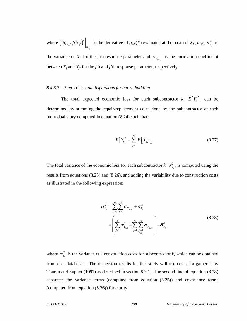
CHAPTER 8 209 Variability of Economic Losses
where 2
,x j
k j jm
g x
is the derivative of gk.j’(X) evaluated at the mean of Xj’, mxj’, 2
jx is
the variance of Xj’ for the j’th response parameter and ,j jx x is the correlation coefficient
between Xj and Xj’ for the jth and j’th response parameter, respectively.
8.4.3.3 Sum losses and dispersions for entire building
The total expected economic loss for each subcontractor k, kE Y , can be
determined by summing the repair/replacement costs done by the subcontractor at each
individual story computed in equation (8.24) such that:
,1
m
k k jj
E Y E Y
(8.27)
The total variance of the economic loss for each subcontractor k, 2
kY , is computed using the
results from equations (8.25) and (8.26), and adding the variability due to construction costs
as illustrated in the following expression:
,
, ,
2 2
1 1
2 2
1 1 1
k kj kj k
k j kj kj k
m m
Y Y Yj j
m m m
Y Y Yj j j
j j
(8.28)
where 2
kY is the variance due construction costs for subcontractor k, which can be obtained
from cost databases. The dispersion results for this study will use cost data gathered by
Touran and Suphot (1997) as described in section 8.3.1. The second line of equation (8.28)
separates the variance terms (computed from equation (8.25)) and covariance terms
(computed from equation (8.26)) for clarity.

CHAPTER 8 210 Variability of Economic Losses
The covariance between economic losses due to work performed subcontractor k
and subcontractor k’, ,k kY
, is a function of both response parameter correlations and
correlations from construction costs. This type of variability can be estimated using the
FOSM method with the following equation:
,
, ,, ,
1 1k k j j j j k k k k
x xj j
m mk j k j
Y x x x x Y Y Y Yj j j j
m m
g g
x x
(8.29)
where kY
is the standard deviation due construction costs for subcontractor k’ and ,k kY Y is
the correlation coefficient between the construction costs of subcontractors k and k’. Both
kY and ,
k kY Y can be determined from construction cost databases similar to the
information described in section 8.3.1. Note that the first term in equation (8.29) is the term
that accounts for the inherent subcontractor loss correlations due EDP variability previously
described in section 8.3.1.1. The second term represents the covariance that results from the
correlations between construction costs of different subcontractors.
The expected economic loss for the entire building conditioned on non-collapse at a
given level of ground motion intensity, E Y , is computed by summing the losses due to
the work performed by each subcontractor such that:
1
l
kk
E Y E Y
(8.30)
where l is the total amount of subcontractors involved in repairing damage due to
earthquakes. Correspondingly, the variance of the loss for the entire building conditioned
on non-collapse at a given level of ground motion intensity, 2Y , can be found by:
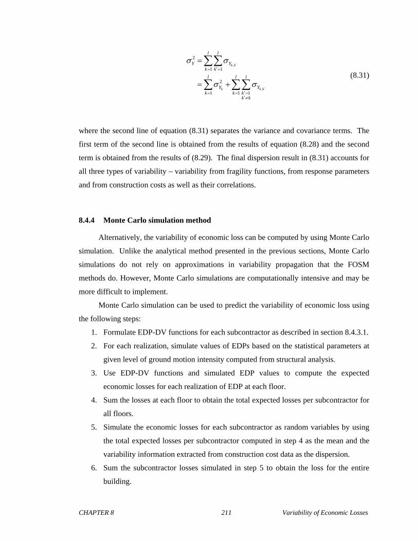
CHAPTER 8 211 Variability of Economic Losses
,
,
2
1 1
2
1 1 1
k k
k k k
l l
Y Yk k
l l l
Y Yk k k
k k
(8.31)
where the second line of equation (8.31) separates the variance and covariance terms. The
first term of the second line is obtained from the results of equation (8.28) and the second
term is obtained from the results of (8.29). The final dispersion result in (8.31) accounts for
all three types of variability – variability from fragility functions, from response parameters
and from construction costs as well as their correlations.
8.4.4 Monte Carlo simulation method
Alternatively, the variability of economic loss can be computed by using Monte Carlo
simulation. Unlike the analytical method presented in the previous sections, Monte Carlo
simulations do not rely on approximations in variability propagation that the FOSM
methods do. However, Monte Carlo simulations are computationally intensive and may be
more difficult to implement.
Monte Carlo simulation can be used to predict the variability of economic loss using
the following steps:
1. Formulate EDP-DV functions for each subcontractor as described in section 8.4.3.1.
2. For each realization, simulate values of EDPs based on the statistical parameters at
given level of ground motion intensity computed from structural analysis.
3. Use EDP-DV functions and simulated EDP values to compute the expected
economic losses for each realization of EDP at each floor.
4. Sum the losses at each floor to obtain the total expected losses per subcontractor for
all floors.
5. Simulate the economic losses for each subcontractor as random variables by using
the total expected losses per subcontractor computed in step 4 as the mean and the
variability information extracted from construction cost data as the dispersion.
6. Sum the subcontractor losses simulated in step 5 to obtain the loss for the entire
building.

CHAPTER 8 212 Variability of Economic Losses
7. Repeat steps 2 to 7 for a large number of realizations.
8. Compute the standard deviation of the loss for all of the realizations
9. Repeat steps 2 to 8 for different levels of ground motion intensity levels.
In this study, dispersion results for the example building using the Monte Carlo
simulation method described above was implemented by assuming lognormal probability
distributions for both the EDP simulations and the subcontractor loss simulations. To
obtain reliable results, 3000 realizations were used to obtain dispersion results at each level
of ground motion intensity.
8.4.5 Evaluation of quality of FOSM approximations
Understanding how well FOSM methods approximate the direct solutions requires
examining the mean-valued Taylor series expansion of ,k jg X evaluated around a point
x , where the random variable X = EDPj | IM. If Y = ,k jL IM , then
22
2
( )( )
2!
!
x x
nn
n x
X xg gY g x X x
x x
X xgx
x n
(8.32)
when n . Expanding the second term, obtains:
2 ( )2 ( )
2 2! !
x x
nn
nx x
g gY g x X x
x x
X x X xg gx
x x n
(8.33)
A first-order approximation truncates higher order terms such that equation (8.33) becomes:

CHAPTER 8 213 Variability of Economic Losses
x x
g gY g x X x
x x
(8.34)
Recognizing that only the second term in equation (8.34) is random and the other terms are
treated as constants, the mean value of Y is computed by applying the expectation operator
as follows:
x x
g gE Y g x E X x
x x
(8.35)
A “mean-centered” FOSM approximation is one that evaluates equation (8.35) by choosing
xx m , where xm is the mean of X. Equation (8.35) can be reduced, recognizing that
xE X m , such that:
xE Y g m (8.36)
The corresponding approximate variance of Y can be obtained by:
22Y yE Y m
(8.37)
where ym is the mean value of Y. Recognizing that y xm E Y g m from equation
(8.36), equation (8.35) can be substituted into equation (8.37), which becomes:
2
2Y y
x x
g gE g x X x g m
x x
(8.38)

CHAPTER 8 214 Variability of Economic Losses
Once again choosing xx m , this equation reduces to:
2
2
x x
Y xm m
g gE X m
x x
(8.39)
Rearranging and recognizing that xm
g x is a constant, equation (8.39) becomes:
2
22
x
Y xm
gE X m
x
(8.40)
2
22
2
2
x
x
Y xm
Xm
gE X m
x
g
x
(8.41)
The resulting equation in (8.41) shows the calculation of the derivative of g(X), xm
g x ,
becomes very important in the ability of FOSM to approximate the exact solution of 2Y
well.
FOSM methods rely on approximating nonlinear functions using linear relationships
at the point of interest (which in this case is at the mean of X, xm ). Therefore, the quality
of FOSM approximations is dependent on how nonlinear g(X) is around this point and on
the level of dispersion of X. Figure 8.11 shows examples of two extremes that illustrate this
concept. In Figure 8.11(a), g(X) is linear and the solution the FOSM method yields is exact.
This is because the higher order terms in equation (8.33) are equal to zero for this case.
Conversely, if g(X) is highly nonlinear, as shown in Figure 8.11(b), then the FOSM
approximation deviates from the actual solution. As the nonlinearity of the function

CHAPTER 8 215 Variability of Economic Losses
increases, the values of the higher-order terms in equation (8.33) also increase, resulting in
these deviations.
Y
X
Y = g(X)
X
xx
y
y
g(x)
(a)
Y
X
Y = g(X)
X
xx
y
y
g(x)
Y
X
Y = g(X)
X
xx
y
y
g(x)
(a)
Y
X
Y = g(X)
X
xx
yy
g(x)xm
g
x
(b)
Y
X
Y = g(X)
X
xx
yy
g(x)xm
g
x
Y
X
Y = g(X)
X
xx
yy
g(x)xm
g
x
(b)
Figure 8.11 FOSM approximations (a) linear function (b) non-linear function
The error of FOSM methods can be quantified by applying the expectation operator
to equation (8.33), substituting xx m and rearranging such that:
2 ( )
2 ( )
2 2! !x x
nn
xnm m
E X x E X xg gE Y g m x
x x n
(8.42)
If it is assumed that the first term of this equation is much larger than the other terms and
recognize that 22x E X x , the error becomes:
22
2 2!x
xx
m
gE Y g m
x
(8.43)

CHAPTER 8 216 Variability of Economic Losses
This quantity represents the error in the FOSM approximation of the mean value of Y, E[Y],
however, this error term would also have to be carried through equations (8.38) to (8.41)
when computing the variance of Y. Therefore, this error term also contributes to the
difference between the economic loss variances computed by FOSM and the exact results.
This means that the size of the possible errors using FOSM is not only dependent on the
nonlinearity of g(X) (as represented by the second derivative 22
xmg x ) but also on the
size of the variance of X, 2x .
In order to improve the approximations made by the FOSM methods, an alternative
way of computing the slope of g(X) was investigated. Instead of taking the derivative
locally at the mean of X, the slope was calculated over a larger range of X. A rational range
of X to choose would be one that captures the most probable values of X. One such range
would be the values between the 16th percentile, x0.16, and the 84th percentile, x0.84, or
equivalently, one standard deviation below and above the mean of X (i.e. xm +/- x ). This
alternative method of computing the slope of g(X), x x
x x
m
mg x
, can then be determined as
follows:
0.84 0.16
0.84 0.16
x x
x x
m
m
g x g xg
x x x
(8.44)
where,
0.16
0.84
x x
x x
x m
x m
(8.45)
Using this method of computing the slope of g(X) improved dispersion results because
computing the derivative locally does not capture everything that occurs in g(X) within the
probable region of X (the most likely region of X being between xm +/- x ).
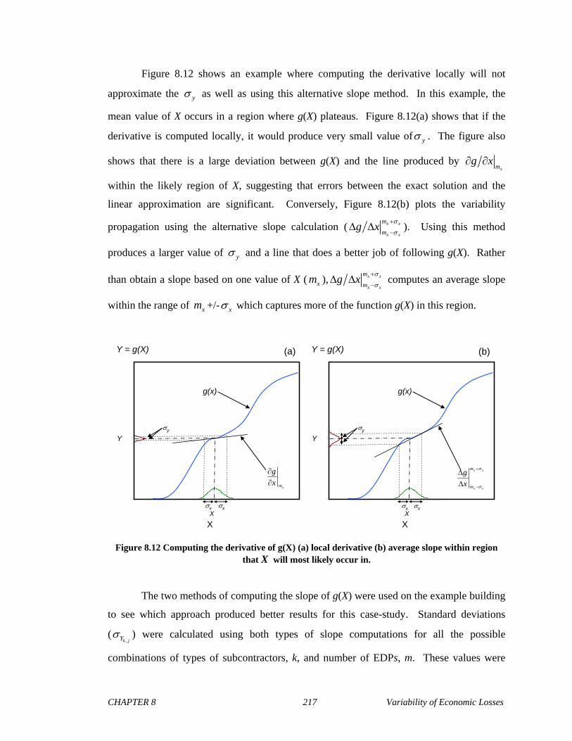
CHAPTER 8 217 Variability of Economic Losses
Figure 8.12 shows an example where computing the derivative locally will not
approximate the y as well as using this alternative slope method. In this example, the
mean value of X occurs in a region where g(X) plateaus. Figure 8.12(a) shows that if the
derivative is computed locally, it would produce very small value of y . The figure also
shows that there is a large deviation between g(X) and the line produced by xm
g x
within the likely region of X, suggesting that errors between the exact solution and the
linear approximation are significant. Conversely, Figure 8.12(b) plots the variability
propagation using the alternative slope calculation ( x x
x x
m
mg x
). Using this method
produces a larger value of y and a line that does a better job of following g(X). Rather
than obtain a slope based on one value of X ( xm ), x x
x x
m
mg x
computes an average slope
within the range of xm +/- x which captures more of the function g(X) in this region.
Y
X
Y = g(X)
Xxx
y
g(x)
xm
g
x
(a)
Y
X
Y = g(X)
Xxx
y
g(x)
xm
g
x
Y
X
Y = g(X)
Xxx
y
g(x)
xm
g
x
(a)
Y
X
Y = g(X)
Xxx
y
g(x)
x x
x x
m
m
g
x
(b)
Y
X
Y = g(X)
Xxx
y
g(x)
x x
x x
m
m
g
x
Y
X
Y = g(X)
Xxx
y
g(x)
x x
x x
m
m
g
x
(b)
Figure 8.12 Computing the derivative of g(X) (a) local derivative (b) average slope within region that X will most likely occur in.
The two methods of computing the slope of g(X) were used on the example building
to see which approach produced better results for this case-study. Standard deviations
(,
k jY ) were calculated using both types of slope computations for all the possible
combinations of types of subcontractors, k, and number of EDPs, m. These values were

CHAPTER 8 218 Variability of Economic Losses
then compared to the corresponding standard deviations obtained from Monte Carlo
simulations, which are considered to be more representative of the exact dispersions.
Table 8.6 shows the standard deviation results of economic loss for each type of
subcontractor and each type of EDP considered at an intensity level equal to the design
basis earthquake using the local derivative to compute the slope of g(X). The top third of
the table shows results using FOSM, the middle third reports the results using simulation
and the bottom third shows the percent difference between the FOSM and simulation
results. Table 8.7 reports the same type of results as Table 8.6, except that the FOSM
standard deviation values were computed using the average slope in equation (8.44). The
results of these two tables show that the slope of g(X) computed using the local derivative
produced larger differences from the simulation results (max = 73%, min = -46%) than
those calculated using the average slope (max = 36%, min = -34%) for this particular
building. Therefore, it was determined that the average slope method would be used to
generate the dispersion results for this building.
Table 8.6 Comparison of standard deviations of economic loss due to EDP variability only using FOSM (local derivative) and simulation methods
IDR1 IDR2 IDR3 IDR4 PFA2 PFA3 PFA4 PFA5 TOTAL
Concrete $21,625 $17,277 $26,964 $39,519 $0 $0 $0 $0 $55,271Masonry $0 $0 $0 $0 $0 $0 $0 $0 $0
Metals $22,625 $21,007 $23,100 $16,294 $0 $0 $0 $0 $41,860Carpentry $0 $0 $0 $0 $0 $0 $0 $0 $0
Moisture Protection $0 $0 $0 $0 $0 $0 $0 $0 $0Doors, Windows, Glass $39,620 $28,181 $25,352 $20,101 $0 $0 $0 $0 $58,401
Finishes $164,433 $122,845 $154,071 $189,000 $45,820 $28,796 $21,177 $9,721 $324,129Mechanical $29,495 $27,006 $23,645 $36,838 $40,483 $13,661 $8,384 $12,769 $74,661
Electrical $84,308 $71,037 $81,100 $119,202 $18,983 $6,406 $3,932 $4,718 $182,701
IDR1 IDR2 IDR3 IDR4 PFA2 PFA3 PFA4 PFA5 TOTAL
Concrete $21,728 $18,072 $21,388 $22,826 $0 $0 $0 $0 $42,242Masonry $0 $0 $0 $0 $0 $0 $0 $0 $0
Metals $19,996 $18,787 $19,530 $11,594 $0 $0 $0 $0 $35,651Carpentry $0 $0 $0 $0 $0 $0 $0 $0 $0
Moisture Protection $0 $0 $0 $0 $0 $0 $0 $0 $0Doors, Windows, Glass $48,215 $34,464 $25,377 $25,237 $0 $0 $0 $0 $68,834
Finishes $135,311 $105,895 $122,839 $121,290 $38,874 $28,582 $22,241 $10,128 $250,981Mechanical $25,285 $23,462 $20,085 $28,617 $55,951 $23,681 $15,619 $21,874 $82,949
Electrical $63,028 $56,544 $60,783 $72,106 $26,237 $11,105 $7,324 $8,083 $131,037
IDR1 IDR2 IDR3 IDR4 PFA2 PFA3 PFA4 PFA5 TOTAL
Concrete 0.00 -0.04 0.26 0.73 N/A N/A N/A N/A 0.31Masonry N/A N/A N/A N/A N/A N/A N/A N/A N/A
Metals 0.13 0.12 0.18 0.41 N/A N/A N/A N/A 0.17Carpentry N/A N/A N/A N/A N/A N/A N/A N/A N/A
Moisture Protection N/A N/A N/A N/A N/A N/A N/A N/A N/ADoors, Windows, Glass -0.18 -0.18 0.00 -0.20 N/A N/A N/A N/A -0.15
Finishes 0.22 0.16 0.25 0.56 0.18 0.01 -0.05 -0.04 0.29Mechanical 0.17 0.15 0.18 0.29 -0.28 -0.42 -0.46 -0.42 -0.10
Electrical 0.34 0.26 0.33 0.65 -0.28 -0.42 -0.46 -0.42 0.39
STANDARD DEVIATTION OF LOSS (FOSM - LOCAL DERIVATIVE)
STANDARD DEVIATTION OF LOSS (SIMULATION)
% DIFFERENCE BETWEEN FOSM & SIMULATION
Subcontractor
Subcontractor
Subcontractor
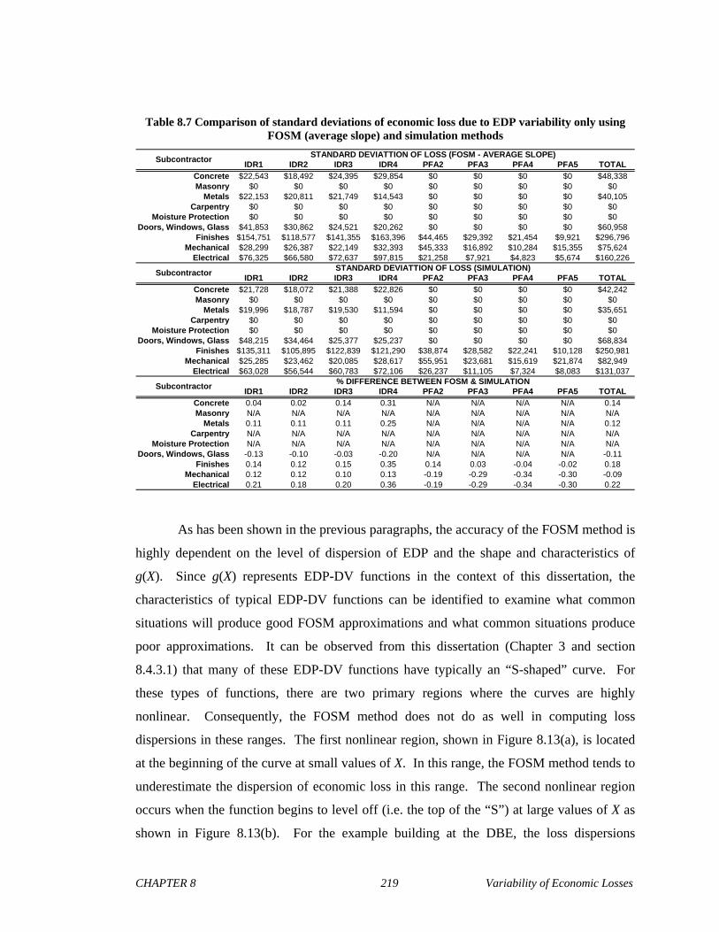
CHAPTER 8 219 Variability of Economic Losses
Table 8.7 Comparison of standard deviations of economic loss due to EDP variability only using FOSM (average slope) and simulation methods
IDR1 IDR2 IDR3 IDR4 PFA2 PFA3 PFA4 PFA5 TOTAL
Concrete $22,543 $18,492 $24,395 $29,854 $0 $0 $0 $0 $48,338Masonry $0 $0 $0 $0 $0 $0 $0 $0 $0
Metals $22,153 $20,811 $21,749 $14,543 $0 $0 $0 $0 $40,105Carpentry $0 $0 $0 $0 $0 $0 $0 $0 $0
Moisture Protection $0 $0 $0 $0 $0 $0 $0 $0 $0Doors, Windows, Glass $41,853 $30,862 $24,521 $20,262 $0 $0 $0 $0 $60,958
Finishes $154,751 $118,577 $141,355 $163,396 $44,465 $29,392 $21,454 $9,921 $296,796Mechanical $28,299 $26,387 $22,149 $32,393 $45,333 $16,892 $10,284 $15,355 $75,624
Electrical $76,325 $66,580 $72,637 $97,815 $21,258 $7,921 $4,823 $5,674 $160,226
IDR1 IDR2 IDR3 IDR4 PFA2 PFA3 PFA4 PFA5 TOTAL
Concrete $21,728 $18,072 $21,388 $22,826 $0 $0 $0 $0 $42,242Masonry $0 $0 $0 $0 $0 $0 $0 $0 $0
Metals $19,996 $18,787 $19,530 $11,594 $0 $0 $0 $0 $35,651Carpentry $0 $0 $0 $0 $0 $0 $0 $0 $0
Moisture Protection $0 $0 $0 $0 $0 $0 $0 $0 $0Doors, Windows, Glass $48,215 $34,464 $25,377 $25,237 $0 $0 $0 $0 $68,834
Finishes $135,311 $105,895 $122,839 $121,290 $38,874 $28,582 $22,241 $10,128 $250,981Mechanical $25,285 $23,462 $20,085 $28,617 $55,951 $23,681 $15,619 $21,874 $82,949
Electrical $63,028 $56,544 $60,783 $72,106 $26,237 $11,105 $7,324 $8,083 $131,037
IDR1 IDR2 IDR3 IDR4 PFA2 PFA3 PFA4 PFA5 TOTAL
Concrete 0.04 0.02 0.14 0.31 N/A N/A N/A N/A 0.14Masonry N/A N/A N/A N/A N/A N/A N/A N/A N/A
Metals 0.11 0.11 0.11 0.25 N/A N/A N/A N/A 0.12Carpentry N/A N/A N/A N/A N/A N/A N/A N/A N/A
Moisture Protection N/A N/A N/A N/A N/A N/A N/A N/A N/ADoors, Windows, Glass -0.13 -0.10 -0.03 -0.20 N/A N/A N/A N/A -0.11
Finishes 0.14 0.12 0.15 0.35 0.14 0.03 -0.04 -0.02 0.18Mechanical 0.12 0.12 0.10 0.13 -0.19 -0.29 -0.34 -0.30 -0.09
Electrical 0.21 0.18 0.20 0.36 -0.19 -0.29 -0.34 -0.30 0.22
STANDARD DEVIATTION OF LOSS (FOSM - AVERAGE SLOPE)
STANDARD DEVIATTION OF LOSS (SIMULATION)
% DIFFERENCE BETWEEN FOSM & SIMULATION
Subcontractor
Subcontractor
Subcontractor
As has been shown in the previous paragraphs, the accuracy of the FOSM method is
highly dependent on the level of dispersion of EDP and the shape and characteristics of
g(X). Since g(X) represents EDP-DV functions in the context of this dissertation, the
characteristics of typical EDP-DV functions can be identified to examine what common
situations will produce good FOSM approximations and what common situations produce
poor approximations. It can be observed from this dissertation (Chapter 3 and section
8.4.3.1) that many of these EDP-DV functions have typically an “S-shaped” curve. For
these types of functions, there are two primary regions where the curves are highly
nonlinear. Consequently, the FOSM method does not do as well in computing loss
dispersions in these ranges. The first nonlinear region, shown in Figure 8.13(a), is located
at the beginning of the curve at small values of X. In this range, the FOSM method tends to
underestimate the dispersion of economic loss in this range. The second nonlinear region
occurs when the function begins to level off (i.e. the top of the “S”) at large values of X as
shown in Figure 8.13(b). For the example building at the DBE, the loss dispersions

CHAPTER 8 220 Variability of Economic Losses
computed in this range using FOSM tend to be overestimated. On the other hand, the
portion of the function located between these two regions is typically much more linear.
Figure 8.13(c) shows this region where the FOSM method will compute a fairly good
approximation of the economic loss dispersion.
Y
X
Y = g(X)
X
xx
y
y
g(x)
(a)
Y
X
Y = g(X)
X
xx
y
y
g(x)
Y
X
Y = g(X)
X
xx
y
y
g(x)
(a)
Y
X
Y = g(X)
X
xx
y
y
g(x)
(b)
Y
X
Y = g(X)
X
xx
y
y
g(x)
Y
X
Y = g(X)
X
xx
y
y
g(x)
(b)
Y
X
Y = g(X)
X
xx
y
y
g(x)
(c)
Y
X
Y = g(X)
X
xx
y
y
g(x)
Y
X
Y = g(X)
X
xx
y
y
g(x)
(c)
Figure 8.13 Typical cases of EDP-DV functions for FOSM approximations (a) under-estimate at small values (b) over-estimate at large values (c) good approximation at
middle values
Figure 8.14 illustrates specific quantitative examples of the different cases discussed
in the previous paragraph using data from the example 4-story building and the EDP-DV
function for repair work done by the electrical subcontractor for drift-sensitive components.
Each graph plots economic loss normalized by the replacement value of the story as a
function of IDR and the slope using both types of methods described previously. The first

CHAPTER 8 221 Variability of Economic Losses
example, shown in Figure 8.14(a), demonstrates what happens for the value of the interstory
drift at the 4th story for a ground motion intensity level equal to an spectral acceleration of
0.25g at the fundamental period (Sa(T1)). The mean value of IDR at this intensity level (mx
= 0.056) occurs in the nonlinear region at the beginning of this EDP-DV function. The
normalized economic loss dispersion computed from Monte Carlo simulation is equal to
0.013 of the replacement value of the story. Using local derivative to compute the slope
( xm
g x = 2.6), also shown in the figure, the FOSM method results in a normalized
economic loss dispersion of 0.0075, which is 42% less than the value calculated using
simulation. If instead the average slope is used ( x x
x x
m
mg x
= 2.9), the normalized
economic loss dispersion is equal to 0.0083 using FOSM and is 35% less than the value
computed using simulation. Both methods of computing the slope for the FOSM approach
significantly underestimates the standard deviation because this region of the EDP-DV
function is highly nonlinear; however, using the average slope method produces results that
are closer to the value computed from simulation.
0.00
0.02
0.04
0.000 0.005 0.010
X = IDR
E[Y] = E[L | IDR]
xm
g
x
x x
x x
m
m
g
x
xmx xm
x xm
0.00
0.02
0.04
0.000 0.005 0.010
X = IDR
E[Y] = E[L | IDR]
xm
g
x
x x
x x
m
m
g
x
xmx xm
x xm
0.00
0.02
0.04
0.06
0.08
0.10
0.000 0.010 0.020 0.030
X = IDR
E[Y] = E[L | IDR]
xm
g
x
x x
x x
m
m
g
x
xm
x xm
x xm
0.00
0.02
0.04
0.06
0.08
0.10
0.000 0.010 0.020 0.030
X = IDR
E[Y] = E[L | IDR]
xm
g
x
x x
x x
m
m
g
x
xm
x xm
x xm
(a) IM = 0.25g (b) IM = 0.80g
Figure 8.14 Quantitative examples of FOSM approximations using the different slope methods
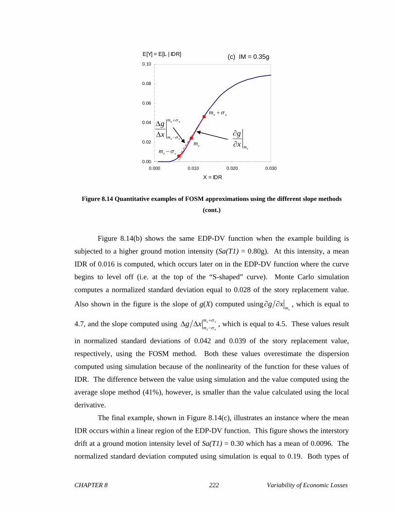
CHAPTER 8 222 Variability of Economic Losses
0.00
0.02
0.04
0.06
0.08
0.10
0.000 0.010 0.020 0.030
X = IDR
E[Y] = E[L | IDR]
xm
g
x
x x
x x
m
m
g
x
xm
x xm
x xm
0.00
0.02
0.04
0.06
0.08
0.10
0.000 0.010 0.020 0.030
X = IDR
E[Y] = E[L | IDR]
xm
g
x
x x
x x
m
m
g
x
xm
x xm
x xm
(c) IM = 0.35g
Figure 8.14 Quantitative examples of FOSM approximations using the different slope methods
(cont.)
Figure 8.14(b) shows the same EDP-DV function when the example building is
subjected to a higher ground motion intensity (Sa(T1) = 0.80g). At this intensity, a mean
IDR of 0.016 is computed, which occurs later on in the EDP-DV function where the curve
begins to level off (i.e. at the top of the “S-shaped” curve). Monte Carlo simulation
computes a normalized standard deviation equal to 0.028 of the story replacement value.
Also shown in the figure is the slope of g(X) computed using xm
g x , which is equal to
4.7, and the slope computed using x x
x x
m
mg x
, which is equal to 4.5. These values result
in normalized standard deviations of 0.042 and 0.039 of the story replacement value,
respectively, using the FOSM method. Both these values overestimate the dispersion
computed using simulation because of the nonlinearity of the function for these values of
IDR. The difference between the value using simulation and the value computed using the
average slope method (41%), however, is smaller than the value calculated using the local
derivative.
The final example, shown in Figure 8.14(c), illustrates an instance where the mean
IDR occurs within a linear region of the EDP-DV function. This figure shows the interstory
drift at a ground motion intensity level of Sa(T1) = 0.30 which has a mean of 0.0096. The
normalized standard deviation computed using simulation is equal to 0.19. Both types of
CHAPTER 8 223 Variability of Economic Losses
slope computational methods approximate values of dispersion closer to the one computed
using simulation. Using the local derivative, the FOSM method calculates the normalized
dispersion to be 20% greater and equal to 0.23. The FOSM method using the average slope
approach computes the normalized standard deviation to be 0.21, which represents a smaller
difference of 8%.
8.5 DISPERSIONS OF ECONOMIC LOSS FOR EXAMPLE 4-STORY BUILDING
The proposed methodology described above was applied to the sample 4-story
reinforced concrete moment resisting frame office building designed by Haselton and
Deierlein (2007). For greater detail on the structural analysis, readers are directed to that
investigation and to Chapter 9 of this dissertation. The building’s mean losses as a function
of seismic intensity (quantified here as spectral acceleration at the fundamental period,
Sa(T1)) is calculated by the loss methodology and assumptions documented in Chapter 3,
and the computer tool described in Chapter 6, was used to generate the loss results for this
study.
Several types of dispersion results were computed and are presented in the next few
sections. Results for dispersions of loss conditioned on non-collapse at a ground motion
intensity level equal to that of the design basis earthquake (DBE, see Chapter 7 for
definition) were computed for each subcontractor. These values were then summed
together to obtain the dispersion of loss due to non-collapse for the entire building. This
computation is repeated for a range of ground motion intensities to obtain dispersion
conditioned on non-collapse as a function of ground motion intensity. The dispersion of the
loss conditioned on collapse was then computed and combined with the results from the
non-collapse values to obtain the total dispersion as a function of ground motion intensity.
The mean and the variability of loss conditioned on ground motion intensity were then
integrated with the site’s hazard curve to obtain the mean annual frequency of exceeding a
particular value of loss. Results from both the analytical and simulation approaches are
presented. The simulation results are considered to be more accurate because of the FOSM
approximations used in the analytical approach. Most of the standard deviation results are
normalized by the building’s replacement value which was calculated to be $12 million as
reported in Chapter 7.
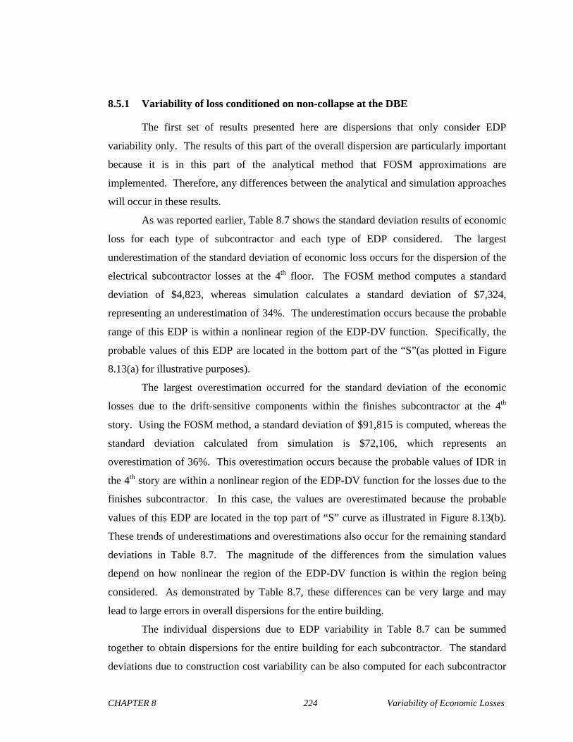
CHAPTER 8 224 Variability of Economic Losses
8.5.1 Variability of loss conditioned on non-collapse at the DBE
The first set of results presented here are dispersions that only consider EDP
variability only. The results of this part of the overall dispersion are particularly important
because it is in this part of the analytical method that FOSM approximations are
implemented. Therefore, any differences between the analytical and simulation approaches
will occur in these results.
As was reported earlier, Table 8.7 shows the standard deviation results of economic
loss for each type of subcontractor and each type of EDP considered. The largest
underestimation of the standard deviation of economic loss occurs for the dispersion of the
electrical subcontractor losses at the 4th floor. The FOSM method computes a standard
deviation of $4,823, whereas simulation calculates a standard deviation of $7,324,
representing an underestimation of 34%. The underestimation occurs because the probable
range of this EDP is within a nonlinear region of the EDP-DV function. Specifically, the
probable values of this EDP are located in the bottom part of the “S”(as plotted in Figure
8.13(a) for illustrative purposes).
The largest overestimation occurred for the standard deviation of the economic
losses due to the drift-sensitive components within the finishes subcontractor at the 4th
story. Using the FOSM method, a standard deviation of $91,815 is computed, whereas the
standard deviation calculated from simulation is $72,106, which represents an
overestimation of 36%. This overestimation occurs because the probable values of IDR in
the 4th story are within a nonlinear region of the EDP-DV function for the losses due to the
finishes subcontractor. In this case, the values are overestimated because the probable
values of this EDP are located in the top part of “S” curve as illustrated in Figure 8.13(b).
These trends of underestimations and overestimations also occur for the remaining standard
deviations in Table 8.7. The magnitude of the differences from the simulation values
depend on how nonlinear the region of the EDP-DV function is within the region being
considered. As demonstrated by Table 8.7, these differences can be very large and may
lead to large errors in overall dispersions for the entire building.
The individual dispersions due to EDP variability in Table 8.7 can be summed
together to obtain dispersions for the entire building for each subcontractor. The standard
deviations due to construction cost variability can be also computed for each subcontractor
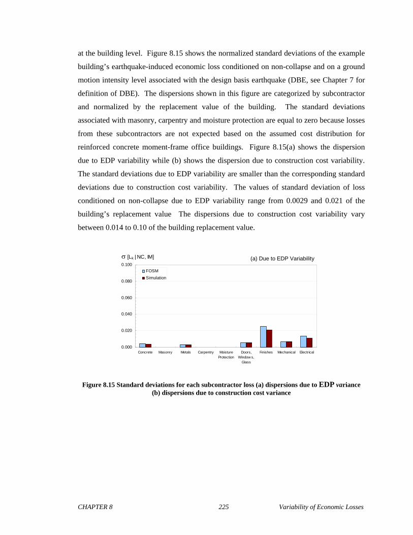
CHAPTER 8 225 Variability of Economic Losses
at the building level. Figure 8.15 shows the normalized standard deviations of the example
building’s earthquake-induced economic loss conditioned on non-collapse and on a ground
motion intensity level associated with the design basis earthquake (DBE, see Chapter 7 for
definition of DBE). The dispersions shown in this figure are categorized by subcontractor
and normalized by the replacement value of the building. The standard deviations
associated with masonry, carpentry and moisture protection are equal to zero because losses
from these subcontractors are not expected based on the assumed cost distribution for
reinforced concrete moment-frame office buildings. Figure 8.15(a) shows the dispersion
due to EDP variability while (b) shows the dispersion due to construction cost variability.
The standard deviations due to EDP variability are smaller than the corresponding standard
deviations due to construction cost variability. The values of standard deviation of loss
conditioned on non-collapse due to EDP variability range from 0.0029 and 0.021 of the
building’s replacement value The dispersions due to construction cost variability vary
between 0.014 to 0.10 of the building replacement value.
0.000
0.020
0.040
0.060
0.080
0.100
Concrete Masonry Metals Carpentry MoistureProtection
Doors,Window s,
Glass
Finishes Mechanical Electrical
FOSM
Simulation
[Lk | NC, IM] (a) Due to EDP Variability
Figure 8.15 Standard deviations for each subcontractor loss (a) dispersions due to EDP variance (b) dispersions due to construction cost variance
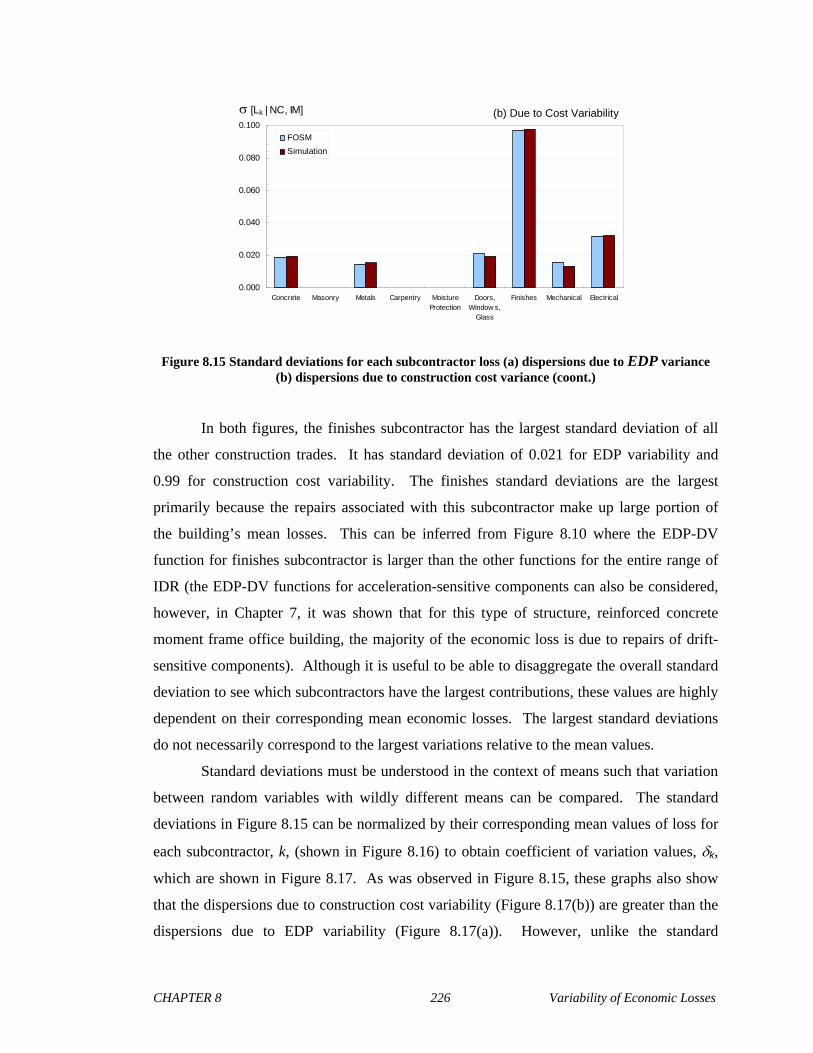
CHAPTER 8 226 Variability of Economic Losses
0.000
0.020
0.040
0.060
0.080
0.100
Concrete Masonry Metals Carpentry MoistureProtection
Doors,Window s,
Glass
Finishes Mechanical Electrical
FOSM
Simulation
[Lk | NC, IM] (b) Due to Cost Variability
Figure 8.15 Standard deviations for each subcontractor loss (a) dispersions due to EDP variance (b) dispersions due to construction cost variance (coont.)
In both figures, the finishes subcontractor has the largest standard deviation of all
the other construction trades. It has standard deviation of 0.021 for EDP variability and
0.99 for construction cost variability. The finishes standard deviations are the largest
primarily because the repairs associated with this subcontractor make up large portion of
the building’s mean losses. This can be inferred from Figure 8.10 where the EDP-DV
function for finishes subcontractor is larger than the other functions for the entire range of
IDR (the EDP-DV functions for acceleration-sensitive components can also be considered,
however, in Chapter 7, it was shown that for this type of structure, reinforced concrete
moment frame office building, the majority of the economic loss is due to repairs of drift-
sensitive components). Although it is useful to be able to disaggregate the overall standard
deviation to see which subcontractors have the largest contributions, these values are highly
dependent on their corresponding mean economic losses. The largest standard deviations
do not necessarily correspond to the largest variations relative to the mean values.
Standard deviations must be understood in the context of means such that variation
between random variables with wildly different means can be compared. The standard
deviations in Figure 8.15 can be normalized by their corresponding mean values of loss for
each subcontractor, k, (shown in Figure 8.16) to obtain coefficient of variation values, k,
which are shown in Figure 8.17. As was observed in Figure 8.15, these graphs also show
that the dispersions due to construction cost variability (Figure 8.17(b)) are greater than the
dispersions due to EDP variability (Figure 8.17(a)). However, unlike the standard

CHAPTER 8 227 Variability of Economic Losses
deviations in Figure 8.15, the finishes subcontractor does not have the largest quantification
of dispersion in either the EDP variability values or construction cost variability values.
The mechanical subcontractor has the largest value of [Lk | NC, IM] for EDP variability
(0.30) and the electrical subcontractor has the largest value for construction cost variability
(0.98). The mechanical subcontractor has the largest variation due to EDP variability
because it has variability from both drift and acceleration-sensitive components. The
concrete subcontractor has the largest variation due to construction cost variability because
that is what the data from the Touran and Suphot (1997) study produced as shown in Table
8.1.
0.00
0.05
0.10
0.15
0.20
0.25
Concrete Masonry Metals Carpentry MoistureProtection
Doors,Window s,
Glass
Finishes Mechanical Electrical
FOSM
Simulation
E [Lk | NC, IM]
Figure 8.16 Mean values of economic loss for each subcontractor at the DBE
CHAPTER 8 228 Variability of Economic Losses
0.00
0.20
0.40
0.60
0.80
1.00
Concrete Masonry Metals Carpentry MoistureProtection
Doors,Window s,
Glass
Finishes Mechanical Electrical
FOSM
Simulation
[Lk | NC, IM] (a) Due to EDP Variability
0.00
0.20
0.40
0.60
0.80
1.00
Concrete Masonry Metals Carpentry MoistureProtection
Doors,Window s,
Glass
Finishes Mechanical Electrical
FOSM
Simulation
[Lk | NC, IM] (b) Due to Cost Variability
Figure 8.17 Coefficient of variations for each subcontractor loss (a) dispersions due to EDP variance (b) dispersions due to construction cost variance
Figure 8.15 and Figure 8.17 also compare dispersion results that were computed
using both the analytical and simulation approach. The dispersion results due to
construction costs show good agreement between the two approaches because the Monte
Carlo simulations are simulating the value of dispersions in Table 8.1 directly. That is, the
variances are not being propagated from one type of dispersion to another. The dispersion
results due to EDP variability do not match up as well as the results due to construction cost
variability because FOSM approximations are used to propagate the EDP variability.
Particularly, the standard deviations of the finishes and electrical subcontractors show the
largest discrepancies between the two methods, with differences of 18% and 22%,
respectively. The analytical results of these subcontractor dispersions do not agree as well
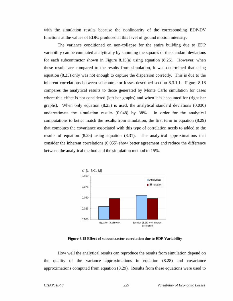
CHAPTER 8 229 Variability of Economic Losses
with the simulation results because the nonlinearity of the corresponding EDP-DV
functions at the values of EDPs produced at this level of ground motion intensity.
The variance conditioned on non-collapse for the entire building due to EDP
variability can be computed analytically by summing the squares of the standard deviations
for each subcontractor shown in Figure 8.15(a) using equation (8.25). However, when
these results are compared to the results from simulation, it was determined that using
equation (8.25) only was not enough to capture the dispersion correctly. This is due to the
inherent correlations between subcontractor losses described section 8.3.1.1. Figure 8.18
compares the analytical results to those generated by Monte Carlo simulation for cases
where this effect is not considered (left bar graphs) and when it is accounted for (right bar
graphs). When only equation (8.25) is used, the analytical standard deviations (0.030)
underestimate the simulation results (0.048) by 38%. In order for the analytical
computations to better match the results from simulation, the first term in equation (8.29)
that computes the covariance associated with this type of correlation needs to added to the
results of equation (8.25) using equation (8.31). The analytical approximations that
consider the inherent correlations (0.055) show better agreement and reduce the difference
between the analytical method and the simulation method to 15%.
0.000
0.025
0.050
0.075
0.100
Equation (8.25) only Equation (8.25) w ith inherentcorrelation
Analytical
Simulation
[L | NC, IM]
Figure 8.18 Effect of subcontractor correlation due to EDP Variability
How well the analytical results can reproduce the results from simulation depend on
the quality of the variance approximations in equation (8.28) and covariance
approximations computed from equation (8.29). Results from these equations were used to
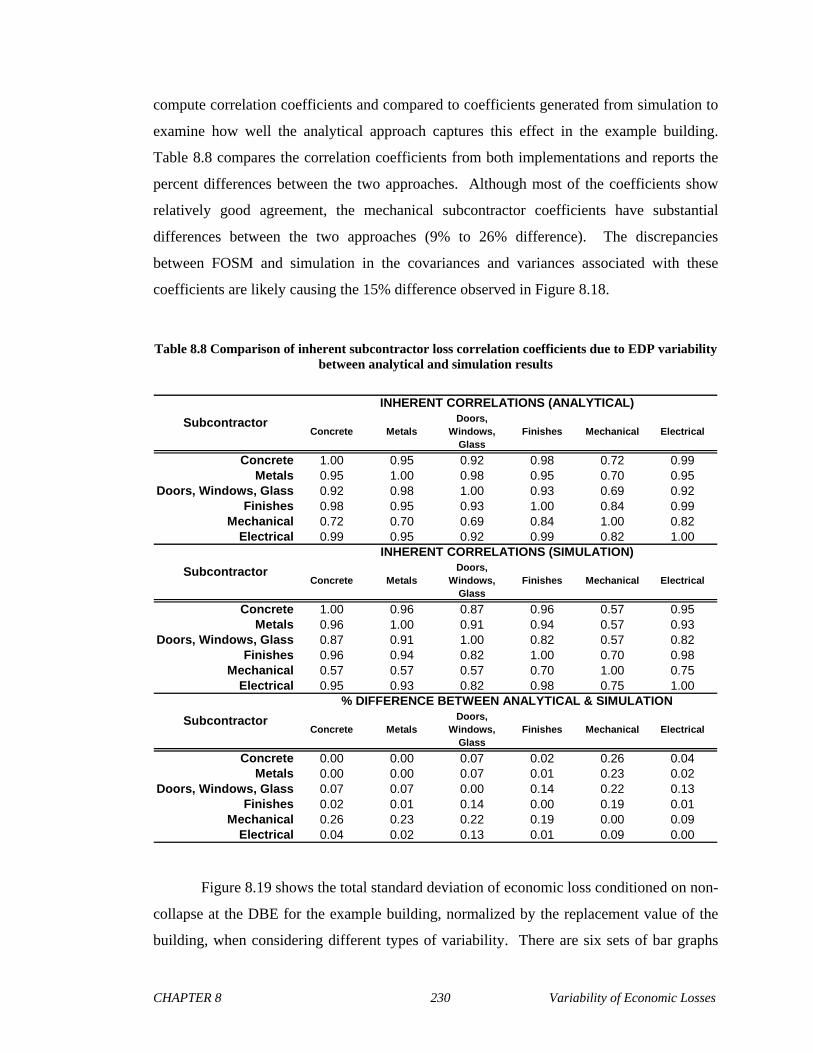
CHAPTER 8 230 Variability of Economic Losses
compute correlation coefficients and compared to coefficients generated from simulation to
examine how well the analytical approach captures this effect in the example building.
Table 8.8 compares the correlation coefficients from both implementations and reports the
percent differences between the two approaches. Although most of the coefficients show
relatively good agreement, the mechanical subcontractor coefficients have substantial
differences between the two approaches (9% to 26% difference). The discrepancies
between FOSM and simulation in the covariances and variances associated with these
coefficients are likely causing the 15% difference observed in Figure 8.18.
Table 8.8 Comparison of inherent subcontractor loss correlation coefficients due to EDP variability between analytical and simulation results
Concrete MetalsDoors,
Windows, Glass
Finishes Mechanical Electrical
Concrete 1.00 0.95 0.92 0.98 0.72 0.99Metals 0.95 1.00 0.98 0.95 0.70 0.95
Doors, Windows, Glass 0.92 0.98 1.00 0.93 0.69 0.92Finishes 0.98 0.95 0.93 1.00 0.84 0.99
Mechanical 0.72 0.70 0.69 0.84 1.00 0.82Electrical 0.99 0.95 0.92 0.99 0.82 1.00
Concrete MetalsDoors,
Windows, Glass
Finishes Mechanical Electrical
Concrete 1.00 0.96 0.87 0.96 0.57 0.95Metals 0.96 1.00 0.91 0.94 0.57 0.93
Doors, Windows, Glass 0.87 0.91 1.00 0.82 0.57 0.82Finishes 0.96 0.94 0.82 1.00 0.70 0.98
Mechanical 0.57 0.57 0.57 0.70 1.00 0.75Electrical 0.95 0.93 0.82 0.98 0.75 1.00
Concrete MetalsDoors,
Windows, Glass
Finishes Mechanical Electrical
Concrete 0.00 0.00 0.07 0.02 0.26 0.04Metals 0.00 0.00 0.07 0.01 0.23 0.02
Doors, Windows, Glass 0.07 0.07 0.00 0.14 0.22 0.13Finishes 0.02 0.01 0.14 0.00 0.19 0.01
Mechanical 0.26 0.23 0.22 0.19 0.00 0.09Electrical 0.04 0.02 0.13 0.01 0.09 0.00
INHERENT CORRELATIONS (ANALYTICAL)
INHERENT CORRELATIONS (SIMULATION)
% DIFFERENCE BETWEEN ANALYTICAL & SIMULATION
Subcontractor
Subcontractor
Subcontractor
Figure 8.19 shows the total standard deviation of economic loss conditioned on non-
collapse at the DBE for the example building, normalized by the replacement value of the
building, when considering different types of variability. There are six sets of bar graphs
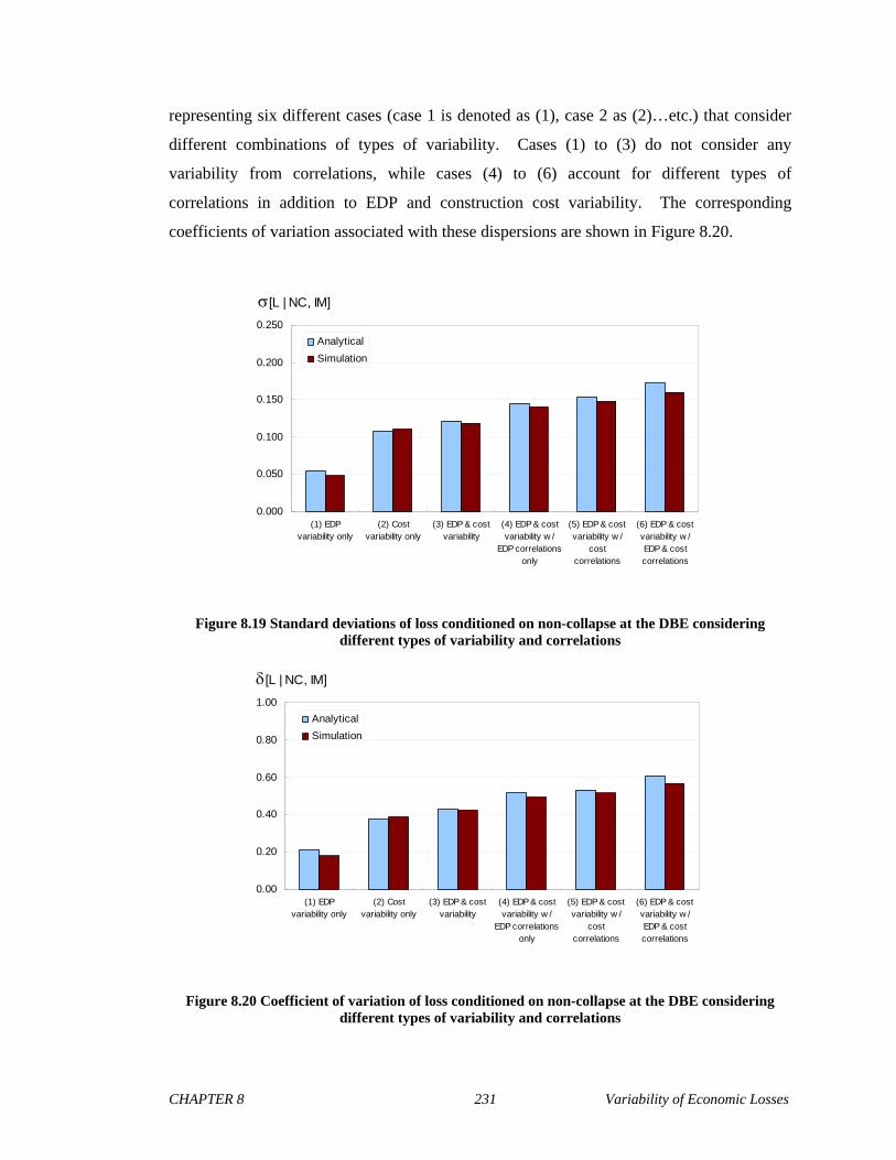
CHAPTER 8 231 Variability of Economic Losses
representing six different cases (case 1 is denoted as (1), case 2 as (2)…etc.) that consider
different combinations of types of variability. Cases (1) to (3) do not consider any
variability from correlations, while cases (4) to (6) account for different types of
correlations in addition to EDP and construction cost variability. The corresponding
coefficients of variation associated with these dispersions are shown in Figure 8.20.
0.000
0.050
0.100
0.150
0.200
0.250
(1) EDPvariability only
(2) Costvariability only
(3) EDP & costvariability
(4) EDP & costvariability w /
EDP correlationsonly
(5) EDP & costvariability w /
costcorrelations
(6) EDP & costvariability w /EDP & costcorrelations
Analytical
Simulation
[L | NC, IM]
Figure 8.19 Standard deviations of loss conditioned on non-collapse at the DBE considering different types of variability and correlations
0.00
0.20
0.40
0.60
0.80
1.00
(1) EDPvariability only
(2) Costvariability only
(3) EDP & costvariability
(4) EDP & costvariability w /
EDP correlationsonly
(5) EDP & costvariability w /
costcorrelations
(6) EDP & costvariability w /EDP & costcorrelations
Analytical
Simulation
[L | NC, IM]
Figure 8.20 Coefficient of variation of loss conditioned on non-collapse at the DBE considering different types of variability and correlations

CHAPTER 8 232 Variability of Economic Losses
Case (1) shows the dispersion when only considering EDP variability, case (2)
shows the dispersion when only construction cost is considered and case (3) shows the
dispersion when both types of variability is considered. The standard deviation due to EDP
variability (0.049) is twice as small as the standard deviation due to construction cost
(0.11). This suggests that the construction cost dispersion has a larger contribution to the
total standard deviation due to both types of variability (case (3)) for this building. It is
important that the variability of construction costs is captured properly, using the type of
cost data available, because this type of variability can be very large and may play a
significant role in the overall variability of economic loss.
The effect of correlations on the dispersions at the DBE is illustrated by cases (4)
to (6) in Figure 8.19. Case (4) considers EDP and construction cost variability with only
the correlations between EDPs, case (5) considers EDP and construction cost variability
with only correlations between construction costs and case (6) considers EDP and
construction cost variability with both EDP and construction cost correlations. All three
cases show that correlations significantly increase the dispersion. EDP correlations increase
the loss dispersion by 20%, whereas construction cost correlations increase the loss
dispersion by 25% when these standard deviations are compared to case (3). When both
types of correlations are accounted for, the standard deviation is 36% larger than the
dispersion value computed without correlations in case (3). This means that the variability
of economic loss conditioned on non-collapse may be substantially underestimated if
correlations due to response parameters and construction costs are ignored.
Each set of bar graphs compares the results generated from the analytical method
with the results from the simulation method. The differences between the two methods
range from as small as 2% (case (2)) to as large as 13% (case (1)). The difference in
standard deviations due to EDP variability between the two methods is fairly significant
because of the FOSM approximations. These differences appear to be decrease when
combined with the variability of construction costs. The construction cost standard
deviations, which show better agreement between the analytical and simulation results,
contribute a larger portion of the total dispersion and, as a result, there is a smaller
difference between the two methods for standard deviations when both sources of
variability are combined.

CHAPTER 8 233 Variability of Economic Losses
8.5.2 Variability of loss conditioned on non-collapse as a function of IM
The analyses to generate results shown in section 8.5.1 were repeated for a range of
seismic intensities to obtain dispersion results as function ground motion intensity. The
standard deviations of economic loss conditioned on non-collapse as function of ground
motion intensity, measured here as spectral acceleration at the fundamental period, Sa(T1),
are shown in Figure 8.21 for six cases that were reported in Figure 8.19. The standard
deviations reported here are normalized by the replacement value of the building. Figure
8.21(a) shows loss dispersions due to EDP variability only, Figure 8.21(b) shows loss
dispersions due to construction cost variability only and Figure 8.21(c) shows loss
dispersions for both EDP and construction cost variability. The remaining three graphs,
Figure 8.21(d), Figure 8.21(e) and Figure 8.21(f), plot the dispersion results for EDP and
construction cost variability when combined with EDP correlations only, with construction
cost correlations only, and with both EDP and cost correlations combined, respectively.

CHAPTER 8 234 Variability of Economic Losses
0.00
0.10
0.20
0.30
0.40
0.0 0.5 1.0 1.5 2.0 2.5 3.0
IM = Sa [g]
[L | IM, NC]
Analytical
Simulation
(b) Cost Variability Only
0.00
0.10
0.20
0.30
0.40
0.0 0.5 1.0 1.5 2.0 2.5 3.0
IM = Sa [g]
[L | IM, NC]
Analytical
Analytical without Inherent Correlation
Simulation
(a) EDP Variability Only
0.00
0.10
0.20
0.30
0.40
0.0 0.5 1.0 1.5 2.0 2.5 3.0
IM = Sa [g]
[L | IM, NC]
Analytical
Simulation
(c) EDP & Cost Variability
0.00
0.10
0.20
0.30
0.40
0.0 0.5 1.0 1.5 2.0 2.5 3.0
IM = Sa [g]
[L | IM, NC]
Analytical
Simulation
(d) EDP & Cost Variability w/ EDP Correlations
0.00
0.10
0.20
0.30
0.40
0.0 0.5 1.0 1.5 2.0 2.5 3.0
IM = Sa [g]
[L | IM, NC]
Analytical
Simulation
(e) EDP & Cost Variability w/ Cost Correlations
0.00
0.10
0.20
0.30
0.40
0.0 0.5 1.0 1.5 2.0 2.5 3.0
IM = Sa [g]
[L | IM, NC]
Analytical
Simulation
(f) EDP & Cost Variability w/ All Correlations
Figure 8.21 Standard deviation of loss conditioned on non-collapse as a function of ground motion intensity (a) EDP variability only (b) construction cost variability only (c) EDP & cost variability
(d) EDP & cost variability with EDP correlations (e) EDP & cost variability with construction cost correlations (f) EDP & cost variability with EDP & cost correlations.

CHAPTER 8 235 Variability of Economic Losses
All six graphs in Figure 8.21 compare the results from the analytical method and the
Monte Carlo simulations. As was observed with the results for the DBE, all six cases show
fairly good agreement between the two methods. The differences between the two methods
are largest for the standard deviations results for EDP variability only. These differences
are slightly larger because of the FOSM approximations that are used to propagate the EDP
variability. The differences occur at ground motion intensity levels that induce values of
EDPs at which the EDP-DV functions that are used to compute loss behave nonlinearly.
The differences between the results of the two methods for the construction cost standard
deviations are entirely due to the variability of the simulations which is dependent on the
number of realizations that are conducted.
Similar trends observed from the results at the DBE can also be observed for the
dispersion results at different levels of ground motion intensity. The standard deviations of
the total loss due to variability in construction costs are substantially larger than those due
to variability in EDP. At higher intensity levels, the standard deviations due to cost
variability can be as much as 3 times the standard deviations due EDP variability. Also
shown in Figure 8.21(a) are economic loss standard deviations computed analytically
without considering the inherent subcontractor loss correlations due work performed on the
same floor/story (section 8.3.1.1). As was the case when examining results at the DBE, the
dispersions of total loss conditioned on non-collapse as a function of ground motion are
significantly underestimated by an average of 30% if these correlations are not accounted
for.
The influence of correlations on the dispersion of economic losses as a function of
ground motion intensity also show similar trends to those observed at the DBE. Figure 8.22
plots and compares the standard deviations of economic loss, normalized by the
replacement value of the building, computed from the simulation results for all six cases.
As was the case for the dispersions at the DBE, the standard deviations that account for
correlations are either equal to or greater than those that do not. This trend holds true for all
values of ground motion intensity for this building. This re-emphasizes the importance of
incorporating correlations into the computation of economic loss uncertainty.

CHAPTER 8 236 Variability of Economic Losses
0.00
0.10
0.20
0.30
0.40
0.0 0.5 1.0 1.5 2.0 2.5 3.0
IM = Sa [g]
[L | IM, NC]
EDP Variability OnlyCost Variability OnlyEDP & Cost Var., No Corr.EDP & Cost Var. w/ EDP Corr.EDP & Cost Var. w/ Cost Corr.EDP & Cost Var.w/ Cost & EDP Corr.
Figure 8.22 Economic loss standard deviations conditioned on non-collapse (normalized by the building replacement value) as a function of ground motion intensity based on the results from the
simulation method.
As will be observed in the next section, economic loss dispersions conditioned on
non-collapse have a larger influence on the overall loss dispersion at smaller ground motion
intensities. Therefore it is important to understand how correlations influence economic
loss dispersions conditioned on non-collapse at these ground motion intensities. Figure
8.23 shows the same results as in Figure 8.22, but only for ground motion intensity levels
that are smaller than Sa(T1) = 1.0g. From this graph, it can be observed that EDP
correlations have a stronger influence at small values of ground motion intensity, while cost
correlations have a larger effect at higher intensities. EDP correlations have a stronger
influence at small ground motion intensities because EDP correlations tend to be higher in
this range of spectral accelerations. EDPs are highly correlated at small intensities because
in this range, a large portion of the building and its components will behave elastically. For
example, displacements and floor accelerations will be strong correlated for initial values of
spectral acceleration as shown in Figure 8.5(b). As the ground motion intensity increases
and the structure begins to exhibit inelastic behavior, the correlation decreases. As the EDP

CHAPTER 8 237 Variability of Economic Losses
correlations decreases, the construction cost correlations start to play a larger role in
increasing the overall dispersion as shown in Figure 8.23.
0.00
0.10
0.20
0.00 0.25 0.50 0.75 1.00
IM = Sa [g]
[L | IM, NC]
EDP Variability OnlyCost Variability OnlyEDP & Cost Var., No Corr.EDP & Cost Var. w/ EDP Corr.EDP & Cost Var. w/ Cost Corr.EDP & Cost Var.w/ Cost & EDP Corr.
Figure 8.23 Economic loss standard deviations conditioned on non-collapse (normalized by the building replacement value) as a function of ground motion intensity for values of Sa(T1) ≤ 1.0g
based on the results from the simulation method.
8.5.3 Variability of loss conditioned on collapse as a function of IM
Up to this point, the variability of loss conditioned on collapse, 2 TL C, has not been
considered. Using the procedure in section 8.4.2 and the data in Table 8.2, this value was
computed to be 0.43 when considering construction cost correlations and 0.27 when cost
correlations were not considered. These values are only due to the variability of
construction costs and do not vary with the level of ground motion intensity. Figure 8.24(a)
show the results for the variability of loss conditioned on non-collapse computed in the
previous section and Figure 8.24 (b) plots the variability of loss conditioned on collapse as
function of ground motion intensity. Each figure plots standard deviations that are
normalized by the replacement value of the building and reports results for two cases:
CHAPTER 8 238 Variability of Economic Losses
dispersions that consider correlations and dispersions that do not consider correlations. The
economic loss dispersions conditioned on collapse are large and are greater than the
dispersions that are conditioned on non-collapse. As was the case with the dispersions
conditioned non-collapse, the dispersions of losses associated with collapse are driven by
the large values of variability due to construction costs. Because both collapse and non-
collapse loss dispersions primarily depend on construction cost variability, it can be inferred
that when these types of dispersions are combined, the total economic loss uncertainty will
also depend largely on the variability of construction costs.
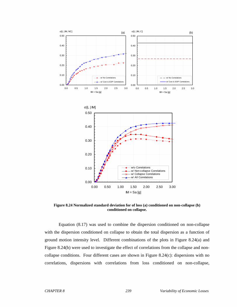
CHAPTER 8 239 Variability of Economic Losses
0.00
0.10
0.20
0.30
0.40
0.50
0.0 0.5 1.0 1.5 2.0 2.5 3.0
IM = Sa [g]
[L | IM, C]
w/ No Correlations
w/ Cost & EDP Correlations
0.00
0.10
0.20
0.30
0.40
0.50
0.0 0.5 1.0 1.5 2.0 2.5 3.0
IM = Sa [g]
[L | IM, NC]
w/ No Correlations
w/ Cost & EDP Correlations
(a) (b)
0.00
0.10
0.20
0.30
0.40
0.50
0.0 0.5 1.0 1.5 2.0 2.5 3.0
IM = Sa [g]
[L | IM, C]
w/ No Correlations
w/ Cost & EDP Correlations
0.00
0.10
0.20
0.30
0.40
0.50
0.0 0.5 1.0 1.5 2.0 2.5 3.0
IM = Sa [g]
[L | IM, NC]
w/ No Correlations
w/ Cost & EDP Correlations
(a) (b)
0.00
0.10
0.20
0.30
0.40
0.50
0.00 0.50 1.00 1.50 2.00 2.50 3.00
IM = Sa [g]
[L | IM]
w/o Correlationsw/ Non-collapse Correlationsw/ Collapse Correlationsw/ All Correlations
Figure 8.24 Normalized standard deviation for of loss (a) conditioned on non-collapse (b) conditioned on collapse.
Equation (8.17) was used to combine the dispersion conditioned on non-collapse
with the dispersion conditioned on collapse to obtain the total dispersion as a function of
ground motion intensity level. Different combinations of the plots in Figure 8.24(a) and
Figure 8.24(b) were used to investigate the effect of correlations from the collapse and non-
collapse conditions. Four different cases are shown in Figure 8.24(c): dispersions with no
correlations, dispersions with correlations from loss conditioned on non-collapse,

CHAPTER 8 240 Variability of Economic Losses
dispersions with correlations from loss condition on collapse and dispersions with
correlations from both the collapse and non-collapse conditions.
At smaller intensity levels, the non-collapse correlations have a larger influence on
the overall dispersion, whereas the collapse correlations have a more substantial effect at
higher intensities. This is an expected result because equation (8.17) is a sum that is
weighted by the probability of collapse, P C IM . At small ground motion intensities,
where the probability of collapse is small, the terms involving the dispersion conditioned on
non-collapse in equation (8.17) are very large compared to the terms involving the
dispersion conditioned on collapse. As P C IM increases with increasing values of
ground motion intensity, collapse plays a larger role in economic losses and its
corresponding dispersion has a larger contribution to the overall variability. Consequently,
the non-collapse correlations are more influential at small ground motion intensities and
collapse correlations are more important at higher ground motion intensities.
8.5.4 Variability of loss as a function of IM & MAF of loss
Figure 8.25 shows the expected losses conditioned on ground motion intensity and
the associated standard deviations for particular values of intensity. The results are
normalized by the replacement value of the building. The seismic intensity associated with
the DBE, is equal to 0.52g. At this intensity, the expected loss is 0.31, with a standard
deviation of 0.21. This means that expected loss could be as small as 0.10 or as large as
0.52 of the building’s replacement value based on a 68% confidence interval (i.e. within
one standard deviation of the mean). This represents a coefficient of variation ([L | IM]) of
0.67.
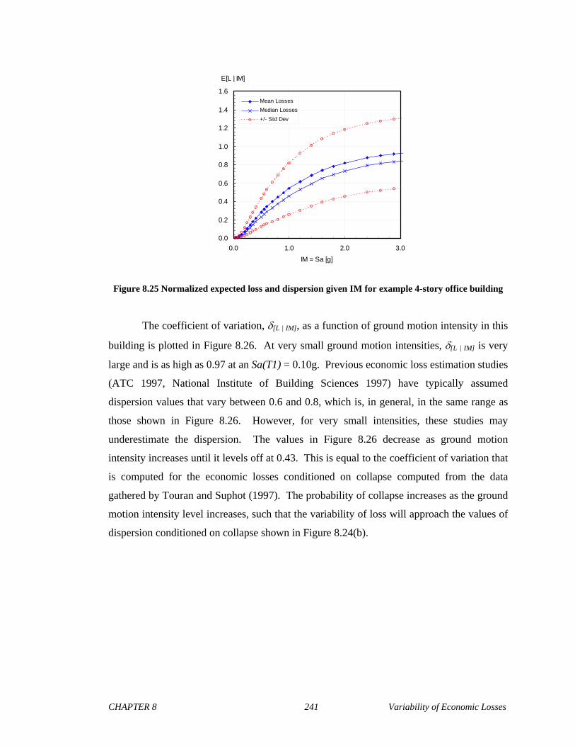
CHAPTER 8 241 Variability of Economic Losses
0.0
0.2
0.4
0.6
0.8
1.0
1.2
1.4
1.6
0.0 1.0 2.0 3.0
IM = Sa [g]
E[L | IM]
Mean Losses
Median Losses
+/- Std Dev
Figure 8.25 Normalized expected loss and dispersion given IM for example 4-story office building
The coefficient of variation, [L | IM], as a function of ground motion intensity in this
building is plotted in Figure 8.26. At very small ground motion intensities, [L | IM] is very
large and is as high as 0.97 at an Sa(T1) = 0.10g. Previous economic loss estimation studies
(ATC 1997, National Institute of Building Sciences 1997) have typically assumed
dispersion values that vary between 0.6 and 0.8, which is, in general, in the same range as
those shown in Figure 8.26. However, for very small intensities, these studies may
underestimate the dispersion. The values in Figure 8.26 decrease as ground motion
intensity increases until it levels off at 0.43. This is equal to the coefficient of variation that
is computed for the economic losses conditioned on collapse computed from the data
gathered by Touran and Suphot (1997). The probability of collapse increases as the ground
motion intensity level increases, such that the variability of loss will approach the values of
dispersion conditioned on collapse shown in Figure 8.24(b).

CHAPTER 8 242 Variability of Economic Losses
0.00
0.20
0.40
0.60
0.80
1.00
1.20
0.00 0.50 1.00 1.50 2.00 2.50 3.00
IM = Sa [g]
[L | IM]
Figure 8.26 Coefficient of variation as a function of intensity level for example building
The results in Figure 8.25 can be integrated with the building site’s hazard curve
using equation (8.16) to obtain values for the mean annual frequency (MAF) of loss. Figure
8.27(a) compares the MAF of loss between economic loss dispersions that consider
correlations and economic loss dispersions that do not consider correlations. The figure
shows that for high probability events that induce losses smaller than $2M, the effect of
correlations is negligible. For losses greater than this value the effect of correlations
becomes much more significant. At a loss of $12M, the assumed mean replacement value
of the building, the MAF of loss is equal to 6.6x10⁻⁵ without considering correlations. This
increases by 110% to 1.4x10⁻⁴ when correlations are considered. This trend is similar to the
results obtained by Aslani and Miranda (2005) and confirms the importance of accounting
for correlations when computing the variability of seismically-induced economic loss.

CHAPTER 8 243 Variability of Economic Losses
1.0E-05
1.0E-04
1.0E-03
1.0E-02
1.0E-01
1.0E+00
$0 $5 $10 $15 $20
Loss [$M]
(L>l)
Simulation
Analytical
1.0E-05
1.0E-04
1.0E-03
1.0E-02
1.0E-01
1.0E+00
$0 $5 $10 $15 $20
Loss [$M]
(L>l)
Losses w ithoutCorrelations
Losses w ithCorrelations
(a) Effect of correlations (b) Analytical vs. Simulation (With Correlations)
1.0E-05
1.0E-04
1.0E-03
1.0E-02
1.0E-01
1.0E+00
$0 $5 $10 $15 $20
Loss [$M]
(L>l)
Simulation
Analytical
1.0E-05
1.0E-04
1.0E-03
1.0E-02
1.0E-01
1.0E+00
$0 $5 $10 $15 $20
Loss [$M]
(L>l)
Losses w ithoutCorrelations
Losses w ithCorrelations
(a) Effect of correlations (b) Analytical vs. Simulation (With Correlations)
Figure 8.27 MAF of loss (a) effect of correlations (b) comparison between analytical and simulation methods
Figure 8.27(b) compares the MAF of loss computed using the analytical approach
with MAF of loss computed using simulation. For this building, there is very little
difference between the loss curves computed from the different methods. This is because
most of the economic loss dispersion calculated in this study was due to the large values of
construction cost variability. This type of variability does not require the use of any FOSM
approximations to propagate uncertainty using the analytical method because they are
already expressed in terms of monetary value and taken directly from cost data. The
contributions of the EDP variability, which rely on FOSM approximations using the
analytical method, are small for this building. Further, the FOSM method, in this particular
case, does a relatively good job of estimating the EDP variability generated from simulation
(as shown in Figure 8.21) because the errors in approximating loss dispersions at each floor
(as reported in Table 8.7) seem to offset each other when they are summed together. There
may be cases in which these errors in dispersion at each floor amplify each other and result
in large errors in total loss dispersion due to EDP variability. This means that the
agreement between the analytical and simulation methods shown in Figure 8.27(b) may not
necessarily always hold true if the errors in EDP variability are large and the contributions
of EDP variability are also large.
CHAPTER 8 244 Variability of Economic Losses
8.6 CONCLUSIONS
A method that computes the variability of seismic-induced economic loss by grouping
the losses by subcontractor and incorporating building-level construction cost dispersions
and correlations was presented. The method is more compatible to the way construction
projects are priced and is better suited to use the type of construction cost data that is
currently available. Two types of implementations of the method, an analytical approach
using FOSM approximations and an approach that used Monte Carlo simulation, were
developed to provide analysts different alternatives on how to propagate variability.
Other issues related to the variability of economic loss that were addressed included
accounting for inherent correlations between subcontractor losses due work performed on
the same floor/story. It was shown that ignoring this type of correlation could significantly
underestimate the variance due to structural response parameters (15% at the DBE for the
example building). The use of the bootstrap sampling method was suggested as a way of
obtaining reliable EDP correlation estimates. It was also demonstrated how the bootstrap
method could be used to evaluate how many number of ground motions are needed in
structural analysis to compute robust EDP correlations. An attempt was also made to
improve the FOSM approximations by proposing an alternative way of computing the slope
of the nonlinear functions (EDP-DV functions) used to propagate response parameter
dispersion. It was determined that computing the slope over the range of values within a
standard deviation of the mean EDP, instead of computing the slope locally at the mean
EDP improved the agreement between results computed by the FOSM approximations and
those generated by simulation for the example building being considered.
Variability results from an example 4-story reinforced concrete moment-frame office
building, taken from previous studies (Haselton and Deierlein, 2007), were computed to
illustrate the use of the new economic loss dispersion methodology. At the DBE, the
coefficient of variation for the example building was computed to be 0.67. This value is
fairly large despite the fact that it does not account for epistemic uncertainty. As was
demonstrated in previous investigations (Aslani and Miranda, 2005) correlations due to
EDP variability and construction cost variability significantly increases the overall value of
dispersion conditioned on ground motion intensity (36% at the DBE). Correlations also
significantly increased the MAF of loss by 110% at a loss greater or equal to the
replacement value of the building ($12 million). When the economic loss dispersion was

CHAPTER 8 245 Variability of Economic Losses
disaggregated, it was determined that the variance due to construction costs had larger
contributions to the overall variability than the variance due to EDPs for this building.
Comparing the results generated from the analytical and the simulation
implementations showed that there was fairly good agreement between the two approaches
for the total dispersion in this particular building. However, when the dispersion is
disaggregated, the standard deviations due to EDP variability for each subcontractor
demonstrated larger deviations between the two implementations. This means that the good
agreement between the approaches of the overall dispersions may be misleading because
the errors at the subcontractor level could be offsetting each other in this particular building.
The differences are also mitigated by the fact that dispersions due to construction costs,
which have better agreement between the two approaches, comprised a larger portion of the
total variability. Although this was true for the example building examined in this study, it
may not necessarily be a general trend for all types of buildings. Further research is needed
to see whether these trends hold for other buildings. Analysts must be aware that despite
the good agreement demonstrated in this particular example building, fairly significant
inaccuracies are possible when using FOSM approximations.

CHAPTER 9 246 Losses due to Demolition given Non-collapse
CHAPTER 9
9 SIGNIFICANCE OF RESIDUAL DRIFTS IN BUILDING EARTHQUAKE LOSS ESTIMATION
This chapter is based on the following publication:
Ramirez, C.M., and Miranda, E. (2009), “Significance of Residual Drifts in Building
Earthquake Loss Estimation,” Earthquake Spectra, (in preparation).
9.1 INTRODUCTION
Observation of the performance of buildings in previous earthquakes indicates that
significant residual displacements may occur. Recent analytical and experimental studies
(Mahin and Bertero 1981, MacRae and Kawashima 1997, Pampanin et al. 2002, Ruiz-
Garcia and Miranda 2005) have shown that the likelihood of experiencing residual
deformations increases as the level of inelastic deformation increases. This suggests that
lateral force resisting systems that are capable of sustaining large lateral displacements are
more likely to experience residual deformations when subjected to seismic ground motions.
Although it has been demonstrated that structural systems with large deformation capacity
do a relatively good job in reducing the probability of collapse in buildings (Haselton and
Deierlein, 2007), these structures are more likely sustain residual drifts that may result in
poor performance when considering other metrics such as economic losses and the loss of
facility use after and earthquake has occurred.
Residual displacements and its consequences play an important role in structural
performance (Ruiz-Garcia & Miranda 2005). In the 1985 Michoacan earthquake, for
instance, numerous reinforced concrete buildings were demolished in Mexico City because
of the complications associated with repairing and straightening the permanent
deformations the structures experienced (Rosenblueth and Meli, 1986). In another example,

CHAPTER 9 247 Losses due to Demolition given Non-collapse
scores of Kobe’s bridge reinforced concrete bridge piers sustained excessive residual
displacements during the Hyogo-Ken-Nambu earthquake, necessitating demolition and
replacement (Kawashima, 2000). In both examples, the structures performed well in terms
of preventing collapse, as they were able to remain standing. However, from a loss
standpoint, these structures exhibited poor structural performance as they had to be
demolished leading not only to large economic losses associated with demolition and
reconstruction, but also with the loss of use of the facility for long periods of time until
reconstruction was completed.
Recent advances in earthquake engineering – particularly the advent of the Pacific
Earthquake Engineering Research Center’s (PEER) performance-based design framework
– have attempted to use economic loss as a performance metric for design. PEER’s
evaluation framework can be traced back to building-specific loss estimation methodologies
first proposed by Scholl et al. (1982). Initially, PEER’s framework was based on methods
that only considered economic losses due to repairable damage given the building has not
collapsed. Monetary losses induced by seismic ground motions are calculated by using
structural response parameters (peak interstory drift, peak floor accelerations…etc.) to
estimate damage in different building components. The cost to repair each damaged
component is then summed for the entire building to obtain the total loss of the building.
This methodology was eventually improved to include economic losses due to building
replacement given that the building has collapsed (Miranda et al. 2004, Aslani and Miranda
2005). However, the current framework does not account for the economic loss due to
demolishing a building that has not collapsed but cannot be repaired because of excessive
residual (permanent) drifts.
The objective of this study is to present an improved loss estimation methodology
that explicitly incorporates losses resulting from having to demolish buildings that have
experienced large residual drifts. The improved methodology is illustrated by evaluating
economic losses in four buildings. The case-study buildings are reinforced concrete
moment-frames structures, whose modeling and response simulation was conducted by
other investigators (Haselton and Deierlein 2007, Liel and Deierlein 2008). In each case
economic losses are estimated with the existing and improved methodologies.

CHAPTER 9 248 Losses due to Demolition given Non-collapse
9.2 METHODOLOGY
PEER’s building specific loss estimation methodology uses the total probability
theorem to compute the expected value of the total economic loss in a building conditioned
on a ground motion intensity IM=im, E[LT | IM], as the weighted sum of expected losses in
two mutually exclusive, collectively exhaustive events. Namely: (1) collapse does not
occur (non-collapse, NC) and damage in the building is repaired, R, (i.e., NC ∩ R); and (2)
collapse occurs and the building is rebuilt, C (Miranda et al. 2004, Aslani and Miranda
2005, Mitrani-Rieser 2007). The expected value of the loss in the building for a given
ground motion intensity IM=im is computed as:
| | , | | |T T TE L IM E L NC R IM P NC R IM E L C P C IM (9.1)
where E[LT | NC ∩ R, IM] is the expected value of the total loss in the building provided
that collapse does not occur (non-collapse) and the building is repaired given that it has
been subjected to earthquakes with a ground motion intensity IM=im, and E[LT | C] is the
expected loss in the building when collapse occurs in the building. The weights on these
two expected losses are P(NC ∩ R | IM) which is the probability that the building will not
collapse and that it will be repaired given that it has been subjected to earthquakes with a
ground motion intensity IM=im, and P(C | IM) is the probability that the structure will
collapse under a ground motion with a level of intensity, im.
Previous investigations have not included the consequence of earthquake damage
when collapse does not occur but the building has to be demolished, D (i.e., NC ∩ D). To
include this effect, this study proposes that a third intermediate term be added to equation
(9.1), to account for economic losses that may result from this outcome. With this term, the
equation becomes:
| | , |
| | | |
T T
T T
E L IM E L NC R IM P NC R IM
E L NC D P NC D IM E L C P C IM
(9.2)

CHAPTER 9 249 Losses due to Demolition given Non-collapse
where E[LT | NC ∩ D] is the expected loss in the building when there is no collapse but the
building needs to be demolished. The weight on this expected loss is P(NC ∩ D | IM),
which is the probability that the building will not collapse but that it has to be demolished,
given that it has been subjected to earthquakes with a ground motion intensity IM=im. As
will be shown later, in many cases, ignoring this term can lead to significant
underestimations of earthquake losses.
The probability that the building will not collapse and that it will be repaired given
that it has been subjected to earthquakes with a ground motion with a level of intensity, im
is given by:
| | , |P NC R IM P R NC IM P NC IM (9.3)
Similarly, the probability that the building will not collapse but that it will be
demolished given that it has been subjected to earthquakes with a ground motion intensity
IM=im can be computed as:
| | , |P NC D IM P D NC IM P NC IM (9.4)
Since the repair and demolition events are mutually exclusive events, given that no
collapse has occurred and collapse and non-collapse are also mutually exclusive events,
then:
| , 1 | ,P R NC IM P D NC IM (9.5)
| 1 |P NC IM P C IM (9.6)
Substituting (9.3)-(9.6) into (9.2) we obtain:

CHAPTER 9 250 Losses due to Demolition given Non-collapse
| | , 1 | , 1 |
| | , 1 | | |
T T
T T
E L IM E L NC R IM P D NC IM P C IM
E L NC D P D NC IM P C IM E L C P C IM
(9.7)
Previous studies (Aslani and Miranda 2005, Mitrani-Rieser 2007) have used a
component-based methodology to calculate E[LT | NC ∩ R, IM]. The damage and
corresponding loss for every component in the building is first calculated, and then summed
up using the following equation:
1
, ,N
T j jj
E L NC IM a E L NC IM
(9.8)
where E[Lj | NC,IM] is the expected normalized loss in the jth component given that global
collapse has not occurred at the intensity level IM, aj is the cost of a new jth component,
and Lj is the normalized loss in the jth component defined as the cost of repair or cost to
replace the component normalized by aj.
A method to simplify the calculation of this term using a story-based approach was
presented in Chapter 3. This approach relies on assumptions about the building’s cost
distribution to calculate loss at each story instead of at every component. If the repair costs
are normalized in the same manner show in equation (9.8), only the value of the story needs
to be specified, rather than the values and quantities of each component. Further,
relationships that relate structural response directly to loss can be developed, such that the
intermediate step of estimating component damage become unnecessary. This approach is
used in this study and the reader is referred to Chapter 3 of this dissertation for further
details of the methodology.
In Equation (9.7) E[LT | C] corresponds to cost of removing the collapse structure
from the site plus the replacement cost of the building. Similarly, E[LT | NC ∩ D] is equal
to the cost of demolishing the existing structure, plus cost of removing debris from the site
plus the replacement cost minus the cost of building components that may be salvageable
because the structure did not collapse.
As shown in Equation (9.7) all three terms are influenced by the probability of
collapse, P(C | IM). Previous studies (e.g., Krawinkler et al. 2005, Haselton and Deierlein

CHAPTER 9 251 Losses due to Demolition given Non-collapse
2007, Liel and Deierlein 2008) have used nonlinear structural simulation models analyzed
using incremental dynamic analysis (Vamvatsikos and Cornell, 2002) to estimate the
probability of collapse as a function of the ground motion intensity. Using a suite of ground
motion records, incremental dynamic analysis captures the effects of variation in frequency
content and other ground motion characteristics, on structural response. The outcome of
incremental dynamic analysis is a set of statistical results that permit the estimation of the
probability of exceedance of critical engineering demand parameters (EDPs) at a number of
ground motion intensities and a collapse fragility function, which describes the probability
of collapse as a function of the ground motion intensity.
In this study, the probability that a structure is forced to be demolished is computed
as a function of the maximum residual interstory drift in the building. The probability that a
building will need to be demolished after an earthquake, given that it has not collapse in an
earthquake with intensity IM =im, can be computed applying the theorem of total
probability as follows:
|0| , | , | ,D RIDRP D NC IM im G D RIDR ridr NC dP RIDR ridr NC IM im
(9.9)
where, GD|RIDR(D | RIDR = ridr, NC) is the cumulative distribution function (CDF) for the
probability that the structure will be demolished, given that the building has not collapsed
but that it has experienced a maximum residual drift is equal to ridr, when subjected to an
earthquake with intensity level, im, and P(RIDR > ridr | NC, IM=im) is the probability of
exceeding ridr given the that the building has not collapsed at the intensity, im. Note that
RIDR is the maximum residual drift in any story in the building. P(RIDR > ridr | NC,
IM=im) can be determined from the structural response simulation similarly to other types
of engineering demand parameters. In this study, GD|RIDR(D | RIDR = ridr, NC) was
assumed to be lognormally distributed. This probability may be interpreted as the
percentage of engineer that would recommend demolition of the building with increasing
levels of residual interstory drift. There is very little data available to obtain an accurate
estimate of the parameters for this probability distribution. For the purposes of this study,
GD|RIDR(D | RIDR = ridr, NC) was assumed to have a median of 1.5% and a lognormal
standard deviation of 0.30. These values were deemed reasonable using engineering
CHAPTER 9 252 Losses due to Demolition given Non-collapse
judgment and a sensitivity analysis was conducted to see how large an influence it had on
estimating losses. The details of this analysis and the reasoning behind the assumed values
are described in section 9.3.3.
9.3 APPLICATIONS
9.3.1 Description of Buildings Studied
To evaluate the influence of the explicit consideration of having to demolish a
building due to excessive residual drifts, four reinforced concrete frame buildings whose
seismic response was previously studied by other investigators were considered. The four
case study buildings are: a 4-story building with ductile detailing, a 12-story building with
ductile detailing, a 4-story building with non-ductile detailing, and a 12-story building with
non-ductile detailing. These buildings are taken from the same sets of structures reported in
Chapter 7. As was described in that chapter, all four structures were assumed to be located
at a site in Los Angeles, CA, south of the city’s downtown area, and is representative of a
typical urban California site with high levels of seismicity, but not subject to near-fault
directivity effects (Haselton et al., 2007). Probabilistic seismic hazard analysis was
conducted by Goulet et al. (2007) to calculate this site’s seismic hazard curve (Figure 7.1),
which provides information on the likelihood of experiencing a ground motion exceeding a
specified intensity. In this study, the spectral acceleration at the first mode period of the
structure, Sa(T1) [g], was used to quantify characterize the ground motion intensity (note
that in the figures and tables in this chapter will denote this value as Sa for brevity,
however, it is implied that this value is at the fundamental period).
The two structures with ductile detailing were modern buildings designed by
Haselton and Deierlein (2007) according to the 2003 International Building Code and
related ACI and ASCE provisions (ACI 2002, ASCE 2002, ICC, 2003). Design spectra for
the site was based on adjusted mapped values of Ss = 1.5g and S1 = 0.6g. Both concrete
frame structures are perimeter, special moment frame structures that comply with capacity
design provisions, strong column-weak beam ratios, joint shear strength and detailing
regulations, in addition to requirements for strength and stiffness. As modeled, the 4-story
building and the 12-story building have fundamental periods of 0.94 and 2.14 seconds,
respectively. Interested readers can refer to Haselton and Deierlein (2007) and Haselton et
CHAPTER 9 253 Losses due to Demolition given Non-collapse
al. (2007) for more details about the designs and modeling parameters of the modern
example structures.
For the structures with non-ductile detailing, the 1967 Uniform Building Code
(UBC 1967) was used to design buildings that were more representative of older concrete
frame structures erected in California from approximately 1950 to 1975. Both designs
complied in accordance with Zone 3 requirements, the highest seismic design provisions of
this era. Although these designs met all requirements of the 1967 UBC (ICBO, 1967) (such
as maximum and minimum reinforcement ratios, maximum stirrup spacing, bar spacing and
anchorage…etc.), these provisions did not require as much transverse reinforcing as modern
day building codes, which result in members that are non-ductile. Further, at the time, no
special provisions for design or reinforcement of beam-column joints were required, and the
strong-column weak beam ratio requirement had yet to be introduced. Thus, these
structures are susceptible to joint-shear failure and column hinging. The buildings are also
much more flexible because of lower reinforcing restrictions and lower seismic design
forces, as demonstrated by their fundamental periods of 2.0 and 2.8 seconds for the 4-story
and 12-story buildings, respectively. Detailed information on the designs and modeling
parameters of these structures can be found in Liel and Deierlein (2008).
Obtaining realistic loss estimations requires developing architectural layouts for the
buildings being considered, to inventory the amount of damageable non-structural
components and to determine the median total replacement cost. This study uses
architectural layouts documented in Mitrani-Reiser (2007) and in Chapter 7 of this
dissertation. A rectangular footprint that is 120-ft wide and by 180-ft long, was used for the
4-story buildings. A smaller layout, with a 120-ft square footprint, was developed for the
12-story buildings. The architectural layouts were used to develop estimates of the total
replacement costs of the buildings. Cost estimates were developed using the RS Means
Cost Estimating Manuals (Balboni, 2007). Table 9.1 lists the estimates for all different
building design variants. Also listed in Table 9.1 are the costs per square foot for each
building design. Although the authors recognize that estimates developed using RS Means
are relatively low compared to typical office building construction costs in the geographical
area being considered, this method follows a rational, systematic approach to estimate
building replacement values. All of the expected loss results that will be presented were
normalized by these values to make valid comparisons within this study.

CHAPTER 9 254 Losses due to Demolition given Non-collapse
Table 9.1Cost estimates for buildings studied
Building Type Footprint Area (sf)Replacement
Cost ($)Cost per
sf ($)4-story 180'x120' 86,400 $12,000,000 $138.89
12-story 120'x120' 172,800 $47,900,000 $277.20
Each of the reinforced concrete frame structures of interest in this study was
modeled in OpenSees (PEER, 2006) using a two-dimensional, three-bay model of the
lateral resisting system and a leaning (P-Δ) column. The model does not incorporate
strength or stiffness from components designed to resist gravity loads. Beams and columns
were modeled with concentrated hinge (lumped plasticity) elements and employ a material
model developed by Ibarra et al. (2005). Haselton and Deierlein (2007) have shown that
the lumped plasticity modeling approach provides reasonable results (compared to fiber-
element models) at low levels of deformation and in addition, captures material
nonlinearities as the structure collapses.
The nonlinear simulation models of reinforced concrete frames were analyzed using
the incremental dynamic analysis technique. The selected ground motions records are from
large magnitude events and recorded at moderate fault-rupture distances on stiff soil or rock
sites (ATC, 2008). The collapse fragility, typically represented by cumulative probability
distribution, was adjusted to account for uncertainties in the structural modeling process and
the expected spectral shape of rare ground motions in California. As an example of the type
simulation data used, the collapse fragility and the EDP data for the ductile, 4-story building
considered in this study are shown in Figure 9.1 and Figure 9.2, respectively. Interested
readers are referred to (Haselton and Deierlein, 2007) for the remaining simulation results
of the example buildings used in this study and for more details on how the structural
simulation was conducted.

CHAPTER 9 255 Losses due to Demolition given Non-collapse
PROBABILITY OF COLLAPSE
0.0
0.2
0.4
0.6
0.8
1.0
0.0 2.0 4.0 6.0
IM = Sa [g]
P(Collapse | IM)
Figure 9.1: Probability of collapse for ductile 4-story reinforced concrete structure (Haselton and Deierlein, 2007)
1
2
3
4
0 0.02 0.04 0.06E[EDP = IDR | IM=Sa]
STORY
2
3
4
5
0 1 2E[EDP = PFA | IM=Sa]
FLOOR
1
2
3
4
0 0.02 0.04E[EDP = RIDR | IM=Sa]
STORY
Sa = 0.05g
Sa = 0.25g
Sa = 0.50g
Sa = 1.00g
Sa = 2.00g
1
2
3
4
0 0.02 0.04 0.06E[EDP = IDR | IM=Sa]
STORY
2
3
4
5
0 1 2E[EDP = PFA | IM=Sa]
FLOOR
1
2
3
4
0 0.02 0.04E[EDP = RIDR | IM=Sa]
STORY
Sa = 0.05g
Sa = 0.25g
Sa = 0.50g
Sa = 1.00g
Sa = 2.00g
1
2
3
4
0 0.02 0.04E[EDP = RIDR | IM=Sa]
STORY
Sa = 0.05g
Sa = 0.25g
Sa = 0.50g
Sa = 1.00g
Sa = 2.00g
Sa = 0.05g
Sa = 0.25g
Sa = 0.50g
Sa = 1.00g
Sa = 2.00g
Figure 9.2: EDP data as a function of building height for ductile 4-story reinforced concrete structure (Haselton and Deierlein, 2007)
9.3.2 Results
The economic loss results at the DBE normalized by the building replacement value
for all four structures considered in this study are summarized in Table 9.2. The normalized
values of each type of loss – non-collapse losses due to repair, non-collapse losses due to
demolition and collapse losses – are reported in columns (1) through (3). Each of the
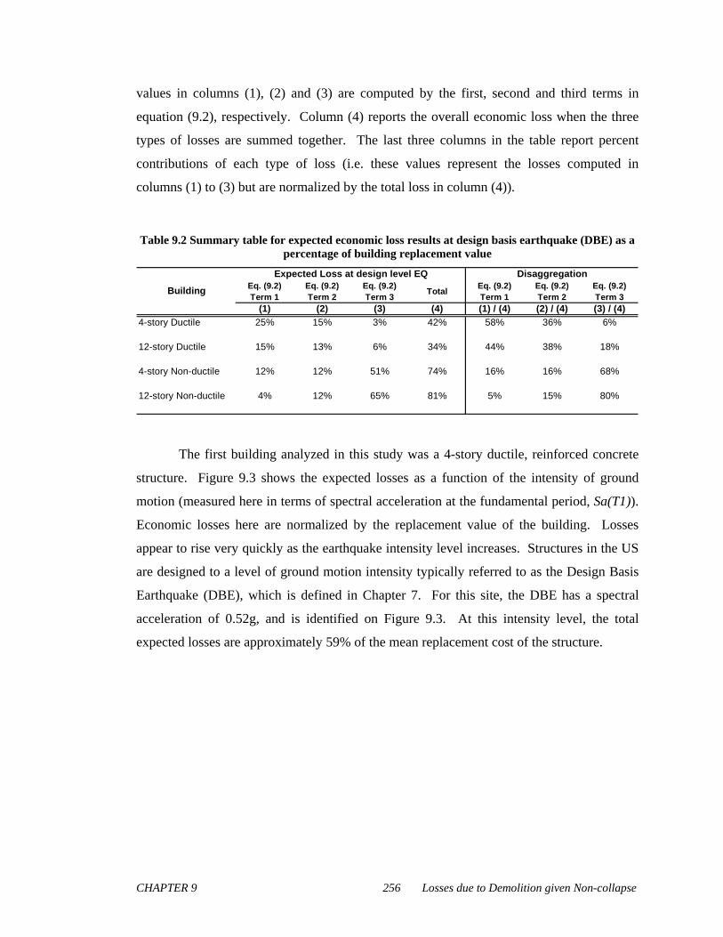
CHAPTER 9 256 Losses due to Demolition given Non-collapse
values in columns (1), (2) and (3) are computed by the first, second and third terms in
equation (9.2), respectively. Column (4) reports the overall economic loss when the three
types of losses are summed together. The last three columns in the table report percent
contributions of each type of loss (i.e. these values represent the losses computed in
columns (1) to (3) but are normalized by the total loss in column (4)).
Table 9.2 Summary table for expected economic loss results at design basis earthquake (DBE) as a percentage of building replacement value
Eq. (9.2) Term 1
Eq. (9.2) Term 2
Eq. (9.2) Term 3
TotalEq. (9.2) Term 1
Eq. (9.2) Term 2
Eq. (9.2) Term 3
(1) (2) (3) (4) (1) / (4) (2) / (4) (3) / (4)
4-story Ductile 25% 15% 3% 42% 58% 36% 6%
12-story Ductile 15% 13% 6% 34% 44% 38% 18%
4-story Non-ductile 12% 12% 51% 74% 16% 16% 68%
12-story Non-ductile 4% 12% 65% 81% 5% 15% 80%
DisaggregationExpected Loss at design level EQ
Building
The first building analyzed in this study was a 4-story ductile, reinforced concrete
structure. Figure 9.3 shows the expected losses as a function of the intensity of ground
motion (measured here in terms of spectral acceleration at the fundamental period, Sa(T1)).
Economic losses here are normalized by the replacement value of the building. Losses
appear to rise very quickly as the earthquake intensity level increases. Structures in the US
are designed to a level of ground motion intensity typically referred to as the Design Basis
Earthquake (DBE), which is defined in Chapter 7. For this site, the DBE has a spectral
acceleration of 0.52g, and is identified on Figure 9.3. At this intensity level, the total
expected losses are approximately 59% of the mean replacement cost of the structure.
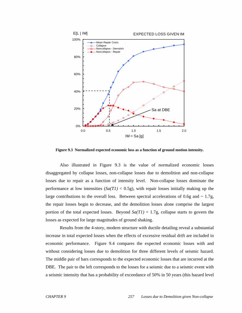
CHAPTER 9 257 Losses due to Demolition given Non-collapse
EXPECTED LOSS GIVEN IM
0%
20%
40%
60%
80%
100%
0.0 0.5 1.0 1.5 2.0
IM = Sa [g]
E[L | IM]
Mean Repair CostsCollapseNoncollapse - DemolishNoncollapse - Repair
Sa at DBE
EXPECTED LOSS GIVEN IM
0%
20%
40%
60%
80%
100%
0.0 0.5 1.0 1.5 2.0
IM = Sa [g]
E[L | IM]
Mean Repair CostsCollapseNoncollapse - DemolishNoncollapse - Repair
Sa at DBE
Figure 9.3 Normalized expected economic loss as a function of ground motion intensity.
Also illustrated in Figure 9.3 is the value of normalized economic losses
disaggregated by collapse losses, non-collapse losses due to demolition and non-collapse
losses due to repair as a function of intensity level. Non-collapse losses dominate the
performance at low intensities (Sa(T1) < 0.5g), with repair losses initially making up the
large contributions to the overall loss. Between spectral accelerations of 0.6g and ~ 1.7g,
the repair losses begin to decrease, and the demolition losses alone comprise the largest
portion of the total expected losses. Beyond Sa(T1) = 1.7g, collapse starts to govern the
losses as expected for large magnitudes of ground shaking.
Results from the 4-story, modern structure with ductile detailing reveal a substantial
increase in total expected losses when the effects of excessive residual drift are included in
economic performance. Figure 9.4 compares the expected economic losses with and
without considering losses due to demolition for three different levels of seismic hazard.
The middle pair of bars corresponds to the expected economic losses that are incurred at the
DBE. The pair to the left corresponds to the losses for a seismic due to a seismic event with
a seismic intensity that has a probability of exceedance of 50% in 50 years (this hazard level
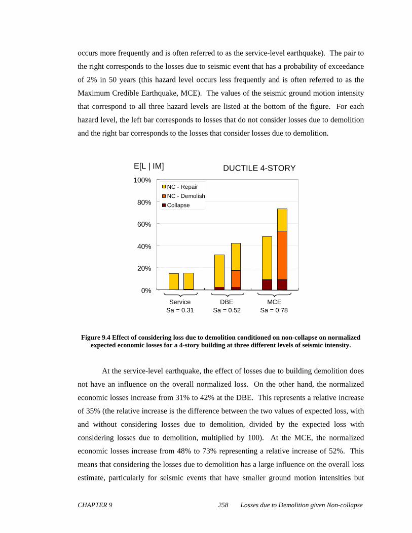
CHAPTER 9 258 Losses due to Demolition given Non-collapse
occurs more frequently and is often referred to as the service-level earthquake). The pair to
the right corresponds to the losses due to seismic event that has a probability of exceedance
of 2% in 50 years (this hazard level occurs less frequently and is often referred to as the
Maximum Credible Earthquake, MCE). The values of the seismic ground motion intensity
that correspond to all three hazard levels are listed at the bottom of the figure. For each
hazard level, the left bar corresponds to losses that do not consider losses due to demolition
and the right bar corresponds to the losses that consider losses due to demolition.
0%
20%
40%
60%
80%
100%NC - Repair
NC - Demolish
Collapse
E[L | IM] DUCTILE 4-STORY
ServiceSa = 0.31
DBESa = 0.52
MCESa = 0.78
0%
20%
40%
60%
80%
100%NC - Repair
NC - Demolish
Collapse
E[L | IM] DUCTILE 4-STORY
ServiceSa = 0.31
DBESa = 0.52
MCESa = 0.78
Figure 9.4 Effect of considering loss due to demolition conditioned on non-collapse on normalized expected economic losses for a 4-story building at three different levels of seismic intensity.
At the service-level earthquake, the effect of losses due to building demolition does
not have an influence on the overall normalized loss. On the other hand, the normalized
economic losses increase from 31% to 42% at the DBE. This represents a relative increase
of 35% (the relative increase is the difference between the two values of expected loss, with
and without considering losses due to demolition, divided by the expected loss with
considering losses due to demolition, multiplied by 100). At the MCE, the normalized
economic losses increase from 48% to 73% representing a relative increase of 52%. This
means that considering the losses due to demolition has a large influence on the overall loss
estimate, particularly for seismic events that have smaller ground motion intensities but
CHAPTER 9 259 Losses due to Demolition given Non-collapse
occur more frequently. At this level of ground motion intensity, the effect of economic
losses due to demolition is even larger than it was at the DBE.
Loss results at these levels were disaggregated to observe how much each term in
equation (9.2) contributes to the overall performance as shown in Figure 9.4 (Loss
disaggregation was performed in a similar manner as documented by Aslani and Miranda,
2005). Each bar in the figure is divided up into collapse losses, non-collapse (NC) losses
due to building demolition and non-collapse losses due to repair costs. The proportions of
each bar are equal to how much each type of loss contributes to the overall loss.
Demolition losses have the largest contributions to the overall loss at the MCE. At this
intensity level, losses conditioned on non-collapse due to demolition represent 60% of the
total loss. This is more than twice as large as the contributions from losses conditioned on
collapse, which comprise 27% of the overall loss at the MCE. The high contributions of
non-collapse losses due to demolition can be explained by comparing the probability of
collapse with the probability of demolition as a function of ground motion intensity, which
is illustrated in Figure 9.5. At the MCE, the probability of demolition is much higher (45%)
than the probability of collapse (8%). This means that the considered structure is more
likely to experience large residual deformations that will lead to demolition, as compared to
collapse due to an earthquake for the given level of ground motion intensity. Consequently,
the non-collapse losses due to demolition are much larger than the losses due to collapse
because the total expected loss is the sum of these two types of losses weighted by the
probability that these events will occur as demonstrated by equation (9.7).

CHAPTER 9 260 Losses due to Demolition given Non-collapse
0.0
0.2
0.4
0.6
0.8
1.0
0.0 0.5 1.0 1.5 2.0 2.5 3.0
IM = Sa / Sa10/50
P(DM = Demolish | IM)
P(DM = Collapse | IM)
P(DM | IM) DUCTILE 4-STORY
IM = Sa / Sa @ DBE
0.0
0.2
0.4
0.6
0.8
1.0
0.0 0.5 1.0 1.5 2.0 2.5 3.0
IM = Sa / Sa10/50
P(DM = Demolish | IM)
P(DM = Collapse | IM)
P(DM | IM) DUCTILE 4-STORY
IM = Sa / Sa @ DBE
Figure 9.5 Comparison of the probability of collapse with the probability of building being demolished due to residual deformation as a function of ground motion intensity.
These results suggest that ignoring the financial consequences of excessive residual
drift can severely underestimate economic loss predictions. Previous loss estimation
methods that do not include these effects may be misleading, predicting better performance
than actually experienced. Performance can be underestimated by as much as 35% at the
DBE and 52% at the MCE as demonstrated by this case-study.
The results in Chapter 7 demonstrated that the effect of building height can have a
substantial influence on predicted economic losses. The effect of building height was also
investigated in this study by comparing the resulting economic losses of the 4-story
structure to the results of a 12-story structure. Figure 9.6 shows the loss results for the 12-
story building at the service-level earthquake, the DBE and the MCE. For each hazard
level, the total normalized economic losses are smaller than the losses of the 4-story
structure shown in Figure 9.4 (Note that the losses are smaller when normalized by the
replacement cost. The replacement costs and losses in the 12-story are larger in
magnitude.). This trend holds whether or not non-collapse losses due to demolition are
considered.

CHAPTER 9 261 Losses due to Demolition given Non-collapse
0%
20%
40%
60%
80%
100%NC - RepairNC - DemolishCollapse
E[L | IM] DUCTILE 12-STORY
ServiceSa = 0.31
DBESa = 0.52
MCESa = 0.78
0%
20%
40%
60%
80%
100%NC - RepairNC - DemolishCollapse
E[L | IM] DUCTILE 12-STORY
ServiceSa = 0.31
DBESa = 0.52
MCESa = 0.78
Figure 9.6 Effect of considering loss due to demolition conditioned on non-collapse on normalized expected economic losses for a 12-story building at three different levels of seismic intensity.
Figure 9.6 also compares the losses with and without considering loss due
demolition, for each hazard level. Despite demonstrating lower total losses, the relative
increase in losses due to considering the effect of demolition losses is larger in the 12-story
structure than it is in the 4-story building. When demolition losses are considered at the
DBE, normalized losses are 45% greater than when the demolition losses are ignored. This
is larger than the 35% increase in normalized loss observed in the loss analysis of the 4-
story structure. This is also true for the MCE, where the relative increase due to demolition
losses is 63% for the 12-story building and only 52% for the 4-story building. This
suggests that large residual drifts may play a more significant role in estimating loss for
high-rise buildings, than it does for low-rise buildings.
The loss results in Figure 9.6 were disaggregated as described previously to
determine the value of contributions from each of the terms in equation (9.2). As was the
case for the 4-story building, demolition losses comprise the largest portion of the overall
loss at the MCE. At this level, losses due to demolition make up 51% of the overall loss.
These case-studies suggest that accounting for excessive residual drift in loss estimations is
important in both low-rise and high-rise structures. Although the proportion of demolition
losses relative to the overall loss is approximately the same in both cases, it was

CHAPTER 9 262 Losses due to Demolition given Non-collapse
demonstrated in the previous paragraph that demolition losses may have a much larger
influence in high-rise buildings than they do in low-rise buildings.
Despite exhibiting larger overall losses, the effects of residual drift on performance
did not have as significant an influence on the older structures (non-ductile detailing) as it
did with the modern structures (ductile detailing). Figure 9.6(a) shows that the total
economic loss at the DBE for a 4-story non-ductile building (74%) is greater than the
corresponding total loss for the ductile 4-story structure reported previously (42%).
However, when comparing the effect of demolition losses, the influence of loss due to
demolition is not as great in the non-ductile structure as it is in the ductile structure. At the
DBE, the increase in loss experienced by the non-ductile building is only 12% while the
increase in the ductile structure is 35%. Similar results can be observed in the non-ductile,
12-story structure as illustrated by Figure 9.6(b). The probability of collapse plays a much
larger role in building performance than the probability of demolition for non-ductile
structures. This can be better demonstrated by examining the deaggregation of these losses.
0%
20%
40%
60%
80%
100%NC - Repair
NC - Demolish
Collapse
E[L | IM] (a) NON-DUCTILE 4-STORY
ServiceSa = 0.31
DBESa = 0.52
MCESa = 0.78
0%
20%
40%
60%
80%
100%NC - Repair
NC - Demolish
Collapse
E[L | IM] (a) NON-DUCTILE 4-STORY
ServiceSa = 0.31
DBESa = 0.52
MCESa = 0.78
0%
20%
40%
60%
80%
100%NC - RepairNC - DemolishCollapse
E[L | IM] (b) NON-DUCTILE 12-STORY
ServiceSa = 0.31
DBESa = 0.52
MCESa = 0.78
0%
20%
40%
60%
80%
100%NC - RepairNC - DemolishCollapse
E[L | IM] (b) NON-DUCTILE 12-STORY
ServiceSa = 0.31
DBESa = 0.52
MCESa = 0.78
Figure 9.7 Loss results for non-ductile buildings studied (a) 4-story (b) 12-story
In addition to showing total losses, Figure 9.7(a) and Figure 9.7(b) also
disaggregates the loss of non-ductile buildings. Comparing these disaggregations with
those shown in Figure 9.4 and Figure 9.6, it can be determined that collapse plays a much
larger role in loss for the non-ductile buildings than it does for the ductile structures.
According to these figures, the contributions of demolition losses to the overall losses are
greatest at the DBE (unlike the ductile structures, where the demolition loss contributions

CHAPTER 9 263 Losses due to Demolition given Non-collapse
were largest at the MCE). However, the demolition loss contributions are much smaller in
these building than they are in the ductile structures (16% for the non-ductile 4-story and
15% for the non-ductile 12-story). Note that the collapse loss contributions are much larger
than the other two types of losses. The 4-story non-ductile structure attributes 86% of its
total loss to collapse, while the 12-story non-ductile structure accredits 89%.
This trend can be explained by observing that the collapse probabilities are much
higher than the probability of demolition. Figure 9.8(a), Figure 9.8(b), Figure 9.8(c) and
Figure 9.8(d) compare the probability of collapse to the probability of building demolition
as a function of ground motion intensity for all four structures. In each plot, ground motion
intensity is normalized by the intensity level of the DBE such that buildings of different
heights can be compared (buildings of different heights typically have different periods and
are designed for different levels of spectral acceleration based on the code-specified design
spectrum). In the ductile structures, the probability of demolition is greater than the
probability of collapse up until 3 times the ground motion intensity of the DBE for the 4-
story building and until 2 times the ground motion intensity of the DBE for the 12-story
building. Conversely, the probability of collapse is significantly larger than the probability
of demolition throughout most of the range of the ground motion intensity levels for both
the 4-story and the 12 story building. Collapse is more likely to occur in the older, non-
ductile buildings for the following reasons: 1) these buildings were designed to withstand
lower seismic forces 2) these buildings are more susceptible to beam-column joint shear
failure, which may result in loss of vertical carrying capacity 3) column hinging is more
likely to occur in these structures because no minimum strong-column, weak-beam
(SCWB) ratio was considered in the design of these buildings 4) column shear failure is
more likely to occur and the plastic hinges developed in these structures will experience fast
degradation due to less confinement and tie reinforcement in non-ductile concrete members.
Because the effect of collapse dominates the monetary losses, the economic consequences
of residual drift had little to no effect on performance for these non-ductile structures.
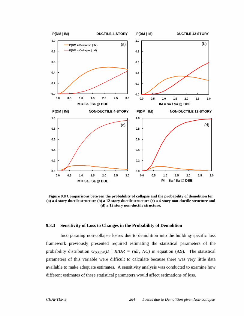
CHAPTER 9 264 Losses due to Demolition given Non-collapse
0.0
0.2
0.4
0.6
0.8
1.0
0.0 0.5 1.0 1.5 2.0 2.5 3.0
IM = Sa / Sa10/50
P(DM = Demolish | IM)
P(DM = Collapse | IM)
P(DM | IM) DUCTILE 4-STORY
0.0
0.2
0.4
0.6
0.8
1.0
0.0 0.5 1.0 1.5 2.0 2.5 3.0
IM = Sa / Sa10/50
P(DM | IM) DUCTILE 12-STORY
0.0
0.2
0.4
0.6
0.8
1.0
0.0 0.5 1.0 1.5 2.0 2.5 3.0
IM = Sa / Sa10/50
P(DM | IM) NON-DUCTILE 4-STORY
0.0
0.2
0.4
0.6
0.8
1.0
0.0 0.5 1.0 1.5 2.0 2.5 3.0
IM = Sa / Sa10/50
P(DM | IM) NON-DUCTILE 12-STORY
(a) (b)
(c) (d)
IM = Sa / Sa @ DBE IM = Sa / Sa @ DBE
IM = Sa / Sa @ DBE IM = Sa / Sa @ DBE
0.0
0.2
0.4
0.6
0.8
1.0
0.0 0.5 1.0 1.5 2.0 2.5 3.0
IM = Sa / Sa10/50
P(DM = Demolish | IM)
P(DM = Collapse | IM)
P(DM | IM) DUCTILE 4-STORY
0.0
0.2
0.4
0.6
0.8
1.0
0.0 0.5 1.0 1.5 2.0 2.5 3.0
IM = Sa / Sa10/50
P(DM | IM) DUCTILE 12-STORY
0.0
0.2
0.4
0.6
0.8
1.0
0.0 0.5 1.0 1.5 2.0 2.5 3.0
IM = Sa / Sa10/50
P(DM | IM) NON-DUCTILE 4-STORY
0.0
0.2
0.4
0.6
0.8
1.0
0.0 0.5 1.0 1.5 2.0 2.5 3.0
IM = Sa / Sa10/50
P(DM | IM) NON-DUCTILE 12-STORY
(a) (b)
(c) (d)
IM = Sa / Sa @ DBE IM = Sa / Sa @ DBE
IM = Sa / Sa @ DBE IM = Sa / Sa @ DBE
Figure 9.8 Comparisons between the probability of collapse and the probability of demolition for (a) a 4-story ductile structure (b) a 12-story ductile structure (c) a 4-story non-ductile structure and
(d) a 12 story non-ductile structure.
9.3.3 Sensitivity of Loss to Changes in the Probability of Demolition
Incorporating non-collapse losses due to demolition into the building-specific loss
framework previously presented required estimating the statistical parameters of the
probability distribution GD|RIDR(D | RIDR = ridr, NC) in equation (9.9). The statistical
parameters of this variable were difficult to calculate because there was very little data
available to make adequate estimates. A sensitivity analysis was conducted to examine how
different estimates of these statistical parameters would affect estimations of loss.
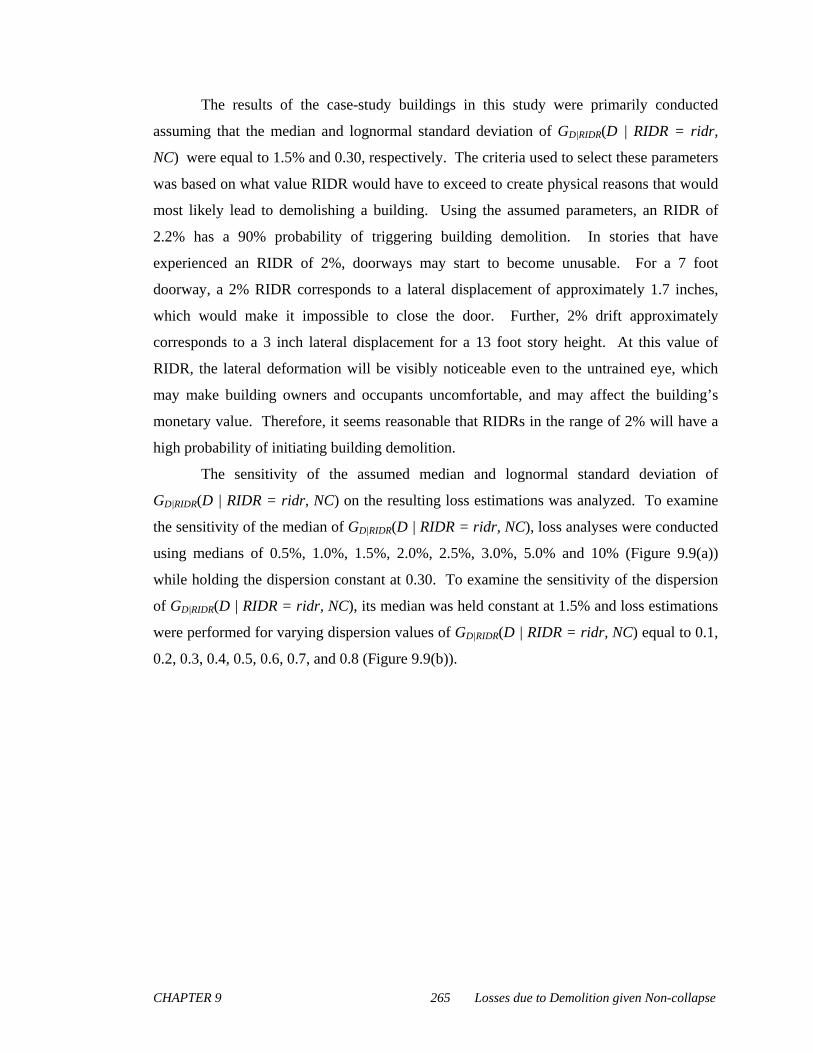
CHAPTER 9 265 Losses due to Demolition given Non-collapse
The results of the case-study buildings in this study were primarily conducted
assuming that the median and lognormal standard deviation of GD|RIDR(D | RIDR = ridr,
NC) were equal to 1.5% and 0.30, respectively. The criteria used to select these parameters
was based on what value RIDR would have to exceed to create physical reasons that would
most likely lead to demolishing a building. Using the assumed parameters, an RIDR of
2.2% has a 90% probability of triggering building demolition. In stories that have
experienced an RIDR of 2%, doorways may start to become unusable. For a 7 foot
doorway, a 2% RIDR corresponds to a lateral displacement of approximately 1.7 inches,
which would make it impossible to close the door. Further, 2% drift approximately
corresponds to a 3 inch lateral displacement for a 13 foot story height. At this value of
RIDR, the lateral deformation will be visibly noticeable even to the untrained eye, which
may make building owners and occupants uncomfortable, and may affect the building’s
monetary value. Therefore, it seems reasonable that RIDRs in the range of 2% will have a
high probability of initiating building demolition.
The sensitivity of the assumed median and lognormal standard deviation of
GD|RIDR(D | RIDR = ridr, NC) on the resulting loss estimations was analyzed. To examine
the sensitivity of the median of GD|RIDR(D | RIDR = ridr, NC), loss analyses were conducted
using medians of 0.5%, 1.0%, 1.5%, 2.0%, 2.5%, 3.0%, 5.0% and 10% (Figure 9.9(a))
while holding the dispersion constant at 0.30. To examine the sensitivity of the dispersion
of GD|RIDR(D | RIDR = ridr, NC), its median was held constant at 1.5% and loss estimations
were performed for varying dispersion values of GD|RIDR(D | RIDR = ridr, NC) equal to 0.1,
0.2, 0.3, 0.4, 0.5, 0.6, 0.7, and 0.8 (Figure 9.9(b)).
CHAPTER 9 266 Losses due to Demolition given Non-collapse
0.0
0.2
0.4
0.6
0.8
1.0
0.0% 1.0% 2.0% 3.0% 4.0%
EDP = RIDR [%]
P(DM=D | RIDR)
0.0
0.2
0.4
0.6
0.8
1.0
0.0% 1.0% 2.0% 3.0% 4.0%
EDP = RIDR [%]
P(DM=D | RIDR)
Figure 9.9 Different distributions for probability of demolition given RIDR (a) Varying the median (b) Varying the dispersion
The economic loss results at the DBE for different values of the median RIDR of
the cumulative probability distribution GD|RIDR(D | RIDR = ridr, NC) are displayed in
Figure 9.10(a). The plot shows that the total loss decreases as the median increases. This
decrease is larger at smaller values of the median than it is at larger values of the median
GD|RIDR(D | RIDR = ridr, NC). Note that as the median is increased and approaches very
large values, the performance is equivalent to the case where demolition losses are not
considered. In this figure, only the value of the repair losses and the demolition losses vary,
whereas the collapse losses remain constant. This is because the statistical parameters of
GD|RIDR(D | RIDR = ridr, NC) only affect the probability of demolition.
A similar, but much weaker trend is observed when using expected annual loss
(EAL) as a metric for performance. Expected annual loss is the average economic loss due
to seismic ground motions that will be incurred each year. It is obtained by integrating
expected losses as a function of ground motion intensity with the site’s seismic hazard
curve (Figure 7.1). Figure 9.10(b) shows the EAL results for the different median values
for the probability of building demolition given RIDR. As was observed in Figure 9.10(a),
the values of loss decrease as the median of GD|RIDR(D | RIDR = ridr, NC) increases. The
decrease in EAL between RIDRs of 0.5% to 2.0%, however, is much smaller than it is for
the expected losses at the DBE. Median values of greater than 2.0% do not produce
differences that are as substantial.
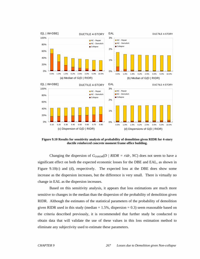
CHAPTER 9 267 Losses due to Demolition given Non-collapse
0%
20%
40%
60%
80%
100%
0.5% 1.0% 1.5% 0.2% 2.5% 3.0% 5.0% 10.0%
(a) Median of G(D | RIDR)
NC - Repair
NC - Demolish
Collapse
E[L | IM=DBE] DUCTILE 4-STORY
0%
1%
2%
3%
0.5% 1.0% 1.5% 0.2% 2.5% 3.0% 5.0% 10.0%
(b) Median of G(D | RIDR)
NC - Repair
NC - Demolish
Collapse
EAL DUCTILE 4-STORY
0%
20%
40%
60%
80%
100%
0.10 0.20 0.30 0.40 0.50 0.60 0.70 0.80
(c) Dispersion of G(D | RIDR)
NC - Repair
NC - Demolish
Collapse
E[L | IM=DBE] DUCTILE 4-STORY
0%
1%
2%
3%
0.5% 1.0% 1.5% 0.2% 2.5% 3.0% 5.0% 10.0%
(d) Dispersionv of G(D | RIDR)
NC - Repair
NC - Demolish
Collapse
EAL DUCTILE 4-STORY
Figure 9.10 Results for sensitivity analysis of probability of demolition given RIDR for 4-story ductile reinforced concrete moment frame office building.
Changing the dispersion of GD|RIDR(D | RIDR = ridr, NC) does not seem to have a
significant effect on both the expected economic losses for the DBE and EAL, as shown in
Figure 9.10(c) and (d), respectively. The expected loss at the DBE does show some
increase as the dispersion increases, but the difference is very small. There is virtually no
change in EAL as the dispersion increases.
Based on this sensitivity analysis, it appears that loss estimations are much more
sensitive to changes in the median than the dispersion of the probability of demolition given
RIDR. Although the estimates of the statistical parameters of the probability of demolition
given RIDR used in this study (median = 1.5%, dispersion = 0.3) seem reasonable based on
the criteria described previously, it is recommended that further study be conducted to
obtain data that will validate the use of these values in this loss estimation method to
eliminate any subjectivity used to estimate these parameters.

CHAPTER 9 268 Losses due to Demolition given Non-collapse
9.3.4 Limitations of results & discussion of residual drift estimations
It is recognized that the resulting economic loss estimates computed in this study
and the conclusions on the influence of residual deformations on seismic-induced economic
loss are dependent on how the values of the RIDR are computed. The simulation results
used in this study were taken from previous research that was conducted on the
performance of reinforced concrete moment frame structures. Although the simulation
techniques were state-of-the-art, the focus of these studies was on collapse performance and
not on capturing residual deformations. It is the opinion of the authors that the RIDR
values computed may be large and possibly overestimated. This is primarily because of the
type of hysteretic model used by Haselton and Deierlein (2007) and Liel and Deierlein
(2008) in their nonlinear simulations. These simulations implemented a material model
developed by Ibarra et al. (2005), which unloads using a stiffness equal to the initial
stiffness. For reinforced concrete members, this may lead to overestimations in residual
displacements as was demonstrated by Ruiz-Garcia and Miranda (2006).
Ruiz-Garcia and Miranda (2006) determined that hysteretic models that capture
stiffness-degradation will compute smaller residual displacements than models that do not
equate the unloading stiffness to the initial stiffness. The decrease in residual displacement
is primarily because stiffness-degradation models have a tendency to unload toward the
origin when subjected to cyclic loading. Systems that do not degrade have larger unloading
stiffness, which resists displacements that would restore the structural member being
modeled back to its original position. Although degrading stiffness systems are more
representative of actual behavior observed by reinforced concrete elements, the model
developed by Ibarra et al. (2005) does not model behavior. This suggests that residual
displacements computed by Haselton and Deierlein (2007) and Liel and Deierlein (2008)
may be overestimated.
If the residual displacements used in this study are overestimated, then the
economic loss results that consider replacement costs due to building demolition will also
be overestimated and may explain why the losses are fairly large. Although the actual
economic loss results may not be as high as those reported in this study, it is still important
to note that considering residual displacements will increase seismic-induced monetary
losses and that this increase may be large.

CHAPTER 9 269 Losses due to Demolition given Non-collapse
9.4 SUMMARY AND CONCLUSIONS
An approach to expand and improve the PEER performance-based design
methodology has been presented. The proposed approach now explicitly takes into account
the fact that a building may have to be demolished after an earthquake. The economic loss
conditioned on the level of ground motion intensity is computed as the sum of three terms:
two terms previously identified corresponding to losses resulting if the building collapses
and to losses associated with repairs given that the structure has not collapsed plus a third
term which accounts for losses resulting from having to demolish buildings that have
experienced excessive residual drifts.
Four case-study buildings were examined to investigate the impact of incorporating
losses due to forced demolition on total economic losses. Results indicate that losses due to
demolition can had a large influence in both the 4-story and the 12-story ductile reinforced
concrete moment-resisting frame buildings that were considered in this study. Including
losses due to demolition increased loss estimates for the DBE event by as much as 45%
larger than the loss estimates that ignored its contribution. This may suggest at that current
methods of loss estimation may be severely underestimating the building performance of
these types of structures by not accounting for the effects of permanent displacement in
structural damage. The influence of demolition losses was not as substantial in the 4-story
and 12-story non-ductile reinforced concrete moment-resisting frame structures. These
building exhibited a much larger probability of collapse at the ground motion intensities of
interest, and consequently yielded economic loss results that were primarily due to collapse.
The proposed approach provides practicing engineers a way of quantifying
differences in building performance between structures with systems that are susceptible to
large permanent deformations and those that use lateral force resisting systems that do not
rely on structure member damage to dissipate energy. The higher economic losses
associated with residual deformation in structures may promote the implementation of self-
centering structural systems that provide alternative means of dealing with excessive
permanent displacement. Although the initial construction cost of these systems may be
larger than that of conventional systems, the ability of these structures to minimize residual
drifts, avoids the potential of demolishing the structure and associate economic costs need
to replace the building.

CHAPTER 9 270 Losses due to Demolition given Non-collapse
The importance of permanent displacement in loss estimation, as illustrated here,
signifies a need for obtaining improved estimates on residual drift. The effect of vertical
permanent displacements should also be examined as they may also lead to building
demolition. Finally, this study limited its evaluation to using expected values of loss,
whereas, there is much value and interest into investigating these issues in terms of other
loss metrics, such as the mean annual frequency of loss.

CHAPTER 10 271 Summary & Conclusions
CHAPTER 10
10 SUMMARY AND CONCLUSIONS
10.1 SUMMARY
Performance-based earthquake engineering (PBEE) has taken tremendous strides in
the past decade. The collaborative effort of PEER researchers has resulted in a methodology
that can quantify structural performance in terms that stakeholders can more readily
understand and use in making decisions regarding seismic risk (e.g. deaths, dollars and
downtime). Unfortunately, evaluating seismic-induced economic loss is no easy task. In
particular, it requires a significant amount of information and is computationally intensive.
Successful adoption of PBEE by practicing engineers may hinge on providing a version of
PEER’s framework that is easier to use and more efficient than previously presented.
This study has presented a new story-based loss estimation methodology, a simplified
implementation of PEER’s previous approaches, as a more efficient way of quantifying
structural seismic performance (Chapter 3). Relationships between structural response and
monetary loss in the form of EDP-DV functions were developed based on the assumptions
on the building’s cost distribution and structural system. Engineers using this method do not
need to conduct the intermediate step of estimating damage, because it has been already
been computed based on assumptions on the building’s cost distribution. Fragility functions
for structural components were developed from experimental data to supplement the
creation of EDP-DV functions (Chapter 4). Generic fragility functions for non-structural
components were generated from empirical data, making it possible to account for the entire
inventory of components in a story when generating EDP-DV functions, yielding more
complete predictions of non-collapse losses (Chapter 5).
These simplifications were implemented into a user-friendly computer tool that can
be used to estimate economic losses as a metric of structural performance (Chapter 6). The

CHAPTER 10 272 Summary & Conclusions
tool was then used to estimate the performance of a set of reinforced concrete moment
resisting frame office buildings to benchmark how much expected losses may be incurred at
a given seismic intensity level, and to evaluate the life-cycle costs due to earthquake
damage (Chapter 7).
This investigation has also proposed a number of improvements to PEER’s loss
estimation methodology to predict better earthquake-induced economic losses. An
alternative method of calculating the uncertainty of predicted losses that incorporates
correlations in construction cost at the building level, rather than at the component-level,
was presented, because dispersion and correlation data for losses on individual components
is not available (Chapter 8). Additionally, an approach was introduced (Chapter 9) that
accounts for losses due to building demolition triggered by excessive permanent
deformations (i.e. residual interstory drift).
10.2 FINDINGS & CONCLUSIONS
10.2.1 Story-based Loss Estimation
Story-based loss estimation, a simplified version of PEER’s previous loss estimation
methodology, is based on creating direct relationships between structural response and loss
by collapsing out the intermediate step of estimating building component damage. These
relationships, termed story EDP-DV functions, were developed for reinforced concrete
moment resisting frame office buildings, by consolidating fragility functions for every
building component and integrating over every damage state for each component. This
integration allows losses to be estimated without knowing the exact cost of repairs if these
values are normalized by the replacement cost of the component. The components can be
summed together at each story without a detailed building inventory, provided that
assumptions can be made about the cost distribution of story based on the building’s
occupancy and use.
Several types of EDP-DV functions for structural components were developed in this
study including functions for ductile and non-ductile reinforced concrete elements. In
general, the functions for ductile components estimated lower losses for a given IDR than
the non-ductile components. The largest change in losses was observed at an IDR of 0.052,
where the losses of ductile concrete components were 140% less than the non-ductile

CHAPTER 10 273 Summary & Conclusions
components. This improved performance is a result of modern building codes requiring
better detailing, such as increasing minimum confinement requirements in order to increase
the member ductility (ACI, 2005). The increase in ductility delays or prevents particular
failure modes (e.g. shear failure of columns, punching shear of slab-column connections,
shear failure of beam-column joints). This reduces the amount economic loss between
ductile and non-ductile members computed by the EDP-DV function between values of
IDR between 0.03 and 0.10.
Consolidating the fragilities and repair costs of building components into story EDP-
DV functions in this manner provides the opportunity to investigate the issue of conditional
damage in spatially-interacting components. In previous studies, when the loss due to
damage of one component is dependent on the damage state of another component, it has
either been ignored leading to an underestimation of losses or double-counted leading to an
overestimation of economic losses. EDP-DV functions were used to examine the
dependency of partitions on pre-Northridge steel beam-column joints by structuring the
functions such that the partitions’ fragilities are conditional on the fragilities of the steel
joints. It was determined that double counting may overestimate the loss significantly while
treating the components as independent underestimates the loss. It was also demonstrated
that as more and more conditional components are accounted for, the underestimation of
independent components becomes more substantial.
Engineers using story-based loss estimation need only provide the economic
investment per story – rather than a detail inventory of all components and their
replacement for the entire story – to calculate loss, making the process much more efficient
and less computationally intensive. Furthermore, performance evaluations are often most
useful during preliminary design – when building inventory is not well defined – because
many important design decisions, such as the structural system, are being determined.
Reducing the amount of computation, time and resources that go into the loss estimation
process using simplified methods allows decision makers to focus on considering the
benefits of the different design alternatives and making better design decisions.
10.2.2 Improved Fragilities in support of EDP-DV Function Formulation
Fragility functions were generated from both experimental and empirical data to
supplement the formulation of story EDP-DV functions. Experimental data from testing of

CHAPTER 10 274 Summary & Conclusions
Pre-Northridge beam-column joints was consolidated and used to create fragilities that can
be used to assess loss of buildings supported by steel moment resisting frames constructed
prior to 1994. Fragilities for two damage states, yielding and fracture, were developed based
on the data available. The fragility for fracture is more relevant to loss estimation because
yielding of a steel joint does not typically result in any required repair actions being taken.
The median IDR and corresponding lognormal standard deviation for fracture were 1.85%
and 0.47, respectively. It was also observed that the yielding parameters were dependant on
span-to-depth ratio, and the parameters for fracture were dependent on beam depth.
Relationships to determine median IDRs based on these dependent section properties were
also developed.
Generic fragility functions were created to account for losses from components that
previously did not have fragilities established from experimental data. Empirical data from
damage reports taken during the 1994 Northridge earthquake was combined with response
values from instrumentation and simulation to create motion-damage pairs, to which
lognormal cumulative distribution functions were fitted. Although many types of functions
were generated, the most valuable relationships derived from this investigation were the
results for drift-sensitive and acceleration-sensitive non-structural components, because it
has been shown that they can comprise a large part of overall loss (Aslani and Miranda
2005, Taghavi and Miranda 2003) and there are only a few fragility functions available to
estimate damage for these components. Although most of the data available were for early
stages of damage, identifying when damage initiates is particularly valuable because losses
at low intensities contribute the most when evaluating expected annual losses (EALs). It
was determined that damage initiates at a median IDR of 0.30% and a median PBA of
0.39g’s based on the data from the CSMIP data. When these fragilities were compared to
previous generic fragilities functions created for HAZUS (NIBS, 1999), the empirical
fragilities estimate a median IDR that is 28% less than those approximated by HAZUS.
Conversely, damage initiation for acceleration-sensitive components occurred at a median
value 58% greater than the median value of the HAZUS fragility functions, suggesting that
previous fragilities may overestimate losses.
Generic fragility functions can be used to improve estimates of seismic-induced
losses given that the considered building has not collapsed. Fragility functions have not
been generated for every type of component that may be included in a building’s inventory.
In the absence of functions formulated from experimental data, these generic functions can
CHAPTER 10 275 Summary & Conclusions
be used as an adequate substitute to account for losses due to these components. Although
these functions may not capture some damage behavior that may be component specific,
they are relationships that are based on data taken from earthquake reconnaissance for these
types of items. They are also likely to yield better loss estimations than using functions
based on expert opinion or ignoring the damage due from components that do not have
specific fragilities.
10.2.3 Implementing loss estimation methods into computer tool
The improved and simplified methods described were implemented into an MS
EXCEL based computer tool. Step-by-step instructions on how to use the program were
documented in this study. During the process of developing this computer tool,
implementation challenges were encountered that needed to be addressed such that the
program estimated economic losses as intended by the framework.
10.2.4 Benchmarking losses
The methods and tools developed in this study were used to predict losses for a set
of typical reinforced concrete moment frame office buildings. The group of 30 modern
code-conforming buildings was designed with ductile detailing (e.g. well confined concrete)
by a previous investigation (Haselton and Deierlein, 2007). A brief comparison was made
to a second set of 25 buildings that were designed with non-ductile concrete moment
frames, representative of structures designed in California prior to 1967 (Liel and Deierlein,
2008). The findings and conclusions from these analyses are as follows:
For the ductile structures, expected losses results at the DBE were found
to be a significant percentage of the replacement value, ranging from 13%
to 54%. When a hazard curve from a site in L.A. was considered, the
EAL computed for this set of buildings varied from 0.4% to 3.3%. Both
metrics indicate that the economic losses can be very large considering
that they conform to current US codes. The wide range of results also
demonstrates that US building codes do not provide a consistent level of
monetary loss performance.
Of the code-conforming structural parameters considered in this study,
building height was found to have the largest influence on expected losses

CHAPTER 10 276 Summary & Conclusions
normalized by the replacement value of the building. Taller buildings
experienced less relative monetary loss than shorter buildings because
lateral deformations tend to concentrate in a smaller percentage of stories.
Consequently, high levels of damage are confined to only a few stories as
opposed to being spread throughout the height of the structure.
Although increasing the design SCWB ratio reduced the losses due to
collapse, increasing the ratio beyond a value of 1.2 did not significantly
affect the total expected losses of the ductile structures. On the other
hand, modifying the R-factor had a larger effect on expected losses at the
DBE. If code committees are interested in adjusting code provisions to
limit direct economic losses due to seismic ground motions, this study
suggests that they would be best served by modifying the R-factor.
Designing for life-safety does not necessarily translate to satisfactory
economic loss performance. The parameters of EAL and the MAF of
collapse were found to be uncorrelated for these sets of buildings.
Performance-based design tools provide separate quantifiable metrics to
address collapse risks and economic losses. The ability to quantify both
metrics also provides decision-makers with information to identify and
consider possible tradeoffs between mitigating losses and reducing
collapse risk.
The older, non-ductile reinforced concrete frame buildings performed
significantly worse in terms of economic losses. The losses experienced
by these structures were on average 1.4 times greater than the ductile
buildings. The larger losses are primarily due to larger losses due to
collapse. These frames are more likely to experience sudden, brittle
failures that are associated with non-ductile detailing.
10.2.5 Improved estimates on the uncertainty of loss
An approach that incorporates building-level construction cost dispersions and
correlations, making it more compatible with the way construction cost data is produced
and recorded, was presented. One of the 4-story buildings from the set of structures

CHAPTER 10 277 Summary & Conclusions
evaluated in Chapter 7 was used as an example to illustrate the use of this approach. It was
determined that for this building the coefficient of variation was computed to be 0.67 at the
DBE and a mean annual frequency (MAF) of loss equal 1.4x10⁻⁴ for losses equal to the
replacement value of the building. This MAF is 5.9 times larger than the MAF of collapse
(8.2 x10⁻⁴). This means that for this building, it would be almost 6 times more likely to
experience an economic loss equal to the replacement value than to experience collapse.
The largest source of variability was attributed to the variability of construction costs for
this building. It was also demonstrated that the correlations from building-level construction
costs and EDPs had a substantial influence on the economic loss dispersion, increasing the
MAF of loss by 110% in this building for losses equal or greater to the replacement value of
the example building.
The approach was implemented using both Monte Carlo simulation and first-order,
second-moment methods of estimating uncertainty to evaluate the accuracy as well as
advantages and disadvantages of each method. It was demonstrated that there was fairly
good agreement between the two approaches for the total dispersion for the example
building. However, this trend would not necessarily be true for other buildings because
there were fairly significant discrepancies between the two methods when the economic
loss dispersion due to EDP variability was disaggregated and compared at the story-level
for each subcontractor. The differences between the two methods were primarily due to
errors of the FOSM approximations occurring within the nonlinear regions of EDP-DV
functions used to evaluate the economic loss dispersion. For this particular building, the
errors happen to compensate for each other when the loss per story were summed together,
which resulted in smaller differences between the two methods when the total dispersions
for the entire building were compared. This may not necessarily be the case for other
buildings where these errors may amplify each other (i.e. the errors are additive).
Evaluating the variability of economic loss by dividing the losses into subcontractor
costs resulted in an inherent correlation between losses due to work performed by different
subcontractors that need to be accounted when evaluating dispersions analytically. This
correlation exists because the amount of work performed by each subcontractor on the same
floor/story is dependent on the same response parameters. Consequently, this correlation
occurs even when the EDPs and construction costs are uncorrelated. It was determined that
if this type of correlation is not accounted for, economic loss dispersions computed
CHAPTER 10 278 Summary & Conclusions
analytically could significantly underestimate the variability due EDP variability (by as
much as 15% for the example building).
Finally, the bootstrap method of sampling was presented as a way of obtaining
reliable estimates of EDP correlations. It was also demonstrated how bootstrap confidence
intervals could be employed to evaluate the number of ground motions required to be used
in structural analysis to obtain reliable EDP correlation coefficients. A closed-form solution
taken from statistical theory was presented as a way of computing these confidence
intervals efficiently.
10.2.6 Accounting for Non-collapse losses due to building demolition
To incorporate this new building damage state into PEER’s loss estimation
framework it is necessary to calculate the probability of building demolition given that it
has not collapsed at a ground motion intensity IM=im. It is proposed that this random
variable be computed as a function of two other probabilities: 1) the probability of
demolition given the building has not collapsed and has experienced a certain peak residual
interstory drift, RIDR = ridr, and 2) the probability of experiencing various levels of RIDR
with increasing levels of seismic intensity IM=im. The first probability accounts for the
variability associated with the amount of permanent deformation that will trigger building
demolition. The second probability accounts for the record-to-record variability of residual
drifts which can be determined from structural analysis.
The effect of including this source of economic loss into PEER’s loss estimation
framework was examined, and it was observed that a substantial increase in loss was
experienced in the ductile reinforced concrete moment resisting frame office buildings
analyzed in this study. The 4-story building analyzed in this part of the investigation
showed a relative increase of 35% in expected loss at the design-basis earthquake (DBE)
and an increase of 45% was observed in the 12-story building when compare to equivalent
buildings that do not consider these losses.
The effect of incorporating these types of monetary losses has a greater influence in
taller buildings because permanent lateral deformations are more likely to be higher in these
structures. The higher gravity loads in the lower stories of tall buildings tend to localize
most of the lateral deformation in these lower stories because of P-delta effects, whereas the
deformation is more evenly spread throughout the height of the building for short structures.

CHAPTER 10 279 Summary & Conclusions
This results in a higher probability that larger residual interstory drifts will occur in the
lower stories of tall buildings. It was also determined that the influence of demolition given
non-collapse is much less significant in older structures built with non-ductile reinforced
concrete. The relative increase in loss at the DBE of the 4-story non-ductile structure was
only 12%. This is because at large lateral deformations, non-ductile frames are more likely
to collapse rather than remain standing with significant permanent drifts.
The increase in losses is also found to be strongly dependent on the statistical
parameters (median and dispersion) estimated for the probability of demolition given RIDR.
A sensitivity analysis was conducted to examine how the variation in estimates of these
parameters affects earthquake-induced losses. It was determined that the estimation of the
median is more sensitive than the dispersion. Due to a lack of data, a median RIDR = 1.5%
and a lognormal standard deviation of 0.30 was recommended. These parameters are based
on values of permanent story drift that would likely cause practical problems if the damaged
building continued to be used was not demolished. Using these parameters implies that
approximately 9% of the buildings with a RIDR of 1% would be demolished while
approximately 85% of buildings with a RIDR of 2% would be demolished. The lower value
corresponds to values that make door, windows and elevators stop functioning while the
higher level corresponds to levels that are clearly visible produce significant P-delta effects.
Accounting for losses due to demolition given non-collapse can be used to evaluate
the difference in performance between new innovative structural systems and conventional
systems. Particularly, this new part of the methodology can be used to highlight improved
performance of structures that implement self-centering systems, which prevent permanent
deformations, over systems that use structural damage to dissipate energy.
10.3 FUTURE RESEARCH NEEDS
Although much progress has been made in performance-based earthquake
engineering and building-specific loss estimation, there are many areas that require future
research. Many simplifying assumptions were made during this investigation that
necessitate further development. Many of these future research needs involve data
collection to establish more fragility functions and repair cost relationships, on which EDP-
DV functions are based. There are also aspects of the current loss estimation methodology

CHAPTER 10 280 Summary & Conclusions
that can be further developed and many other aspects of performance loss results that can be
extended.
10.3.1 Data collection for fragility functions and repair costs
The introduction of PEER’s performance-based earthquake engineering framework
has established the types of data that need to be collected from experiments, construction
cost databases or post-earthquake reconnaissance. Data of particular interest as it relates to
this study include the following:
Experimental data for fragility function development is ongoing such that
damage can be estimated for common types of components that may be found
in a building’s inventory. These fragilities can then be used to create EDP-DV
functions for story-based building-specific loss estimation. Having a complete
set of fragility functions will improve loss estimations by reducing the reliance
on generic fragilities and functions based on expert opinion.
Correlations between fragilities were assumed to be uncorrelated; however, this
needs to be validated by further investigation. Incorporating correlations
quantitatively is complicated because fragility function damage states are
discrete rather than continuous. A method of capturing these fragility function
correlations despite this complication needs to be developed. Once a
methodology has been established, a way of obtaining the value of these
correlations needs to be developed.
Non-collapse losses depend heavily on the values of component repair costs
and how they are formulated. One of the principles that the story-based loss
estimation method relies on is the relative costs of components’ repair costs to
the replacement value of said component. Although there have been some
attempts by previous studies to establish these values, many components still
lack this information and assumptions on their values needed to be made to
complete this study.
Computing the uncertainty of the estimated expected economic losses as
presented in this dissertation necessitates establishing how the replacement
value of each building component is distributed between the different

CHAPTER 10 281 Summary & Conclusions
subcontractors that participate in its construction. Developing relationships
between components costs and subcontractor costs will bridge the gap between
damage estimation (which is typically conducted per component) and the
available construction cost data (which is typically expressed at the building
level).
The dispersion and correlation data presented in Chapter 8 was based on data
that only considered commercial office buildings. Similar studies that gather
this type data for other structural classification types are necessary to compute
the variability of economic loss for other building occupancies.
Statistical data on the values residual interstory drift that trigger building
demolition. This data can then be used to establish the probability
distribution parameters used in Chapter 9 to account for economic losses
due to building demolition.
EDP-DV functions for other building types need to be established to
evaluate the economic losses for structures of all types of classifications.
Functions that consider different structural systems and different
occupancies need to be developed such that computer tools, like the one
presented in Chapter 6, can offer a broad library of functions for users to
choose from.
10.3.2 Improvements to building-specific loss estimation methodology
There are several areas in building-specific loss estimation that require further
development. These areas include the following:
The economic losses presented in this investigation and other recent building-
specific losses estimation studies are typically larger than those computed using
regional loss estimation methods. Validation studies using data collected from
previous and future earthquakes can be used to identify parts of the
methodology, if any, that may not capture the computation of earthquake-
induced economic losses well.
The concepts and framework presented in this dissertation for the computation
of economic losses can be extended to the calculation of fatalities and facility
CHAPTER 10 282 Summary & Conclusions
downtime caused by seismic events. The same basic framework and
probabilistic concepts used the compute of economic losses can be applied to
these other metrics and used to gage performance. Although there have been
studies that have addresses these types of losses (Liel and Deierlein 2008,
Mitrani-Reiser 2007), there has not been as much work conducted in these areas
as there has been in economic losses.
The methodology to compute the variability of economic losses in this
dissertation was limited to aleatoric uncertainty. Modeling uncertainty
associated with the variability of EDPs was not considered in this study. The
incorporation of epistemic uncertainty and its propagation into the building-
specific loss estimation as it relates to the variability associated with structural
response has been previously investigated, however, has not been combined
with the aleatoric findings in this dissertation. This type of uncertainty needs to
be accounted for to obtain a better value of dispersion and to see which type of
uncertainty has the larger contribution to the overall variability.
REFERENCES 283 Introduction
REFERENCES
ACI (2002). Building Code Requirements for Structural Concrete (ACI 318), American Concrete Institute.
Algermissen, S.T., Rinehart, W.A., Dewey, J., Steinbrugge, K.V., Degenkolb, H.J., Cluff, L.S., McClure, F.E., Gordon, R.F. (1972). A study of earthquake losses in the San Francisco bay area: data and analysis. Rockville, MD: Environmental Research Laboratories of National Oceanic & Atmospheric Administration, prepared for the Office of Emergency Preparedness: U.S. Department of Commerce.
Anderson, J.C., and Linderman, R.R. (1991). Steel Beam to Box Column Connections, Report No. CE 91-03. Los Angeles, CA : Department of Civil Engineering, University of Southern California.
Anagnos, T., Rojahn, C., and Kiremidjian, A. (1995). NCEER-ATC Joint Study on Fragility of Buildings, Technical Report NCEER-95-0003. State University of New York at Buffalo: National Center for Earthquake Engineering Research.
ASCE (2002). Minimum Design Loads for Buildings and Other Structures (ASCE 7-02). Reston, VA: American Society of Civil Engineers.
ASCE (2007). Seismic Rehabilitation of Existing Buildings (ASCE/SEI 41-06). Reston, VA: American Society of Civil Engineers.
Aslani, H., and Miranda, E. (2004). “Component-Level and System-Level Sensitivity Study for Earthquake Loss Estimation.” 13th World Conference on Earthquake Engineering (Paper No. 1070). Vancouver, B.C., Canada.
Aslani, H. and Miranda, E. (2005). Probabilistic Earthquake Loss Estimation and Loss Disaggregation in Buildings, Report No. 157. Stanford, CA: John A. Blume Earthquake Engineering Center, Stanford University.
ATC (1985). Earthquake Damage Evaluation Data for California, ATC-13 Report. Redwood City, CA: Applied Technology Council.
ATC (2000). Database on the Performance of Structures Near Strong-Motion Recordings: 1994 Northridge, California, Earthquake, ATC-38 Report. Redwood City, CA.: Applied Technology Council.
ATC (2007). Guidelines for Seismic Performance Assessment of Buildings, ATC-58 Report 35% Draft. Redwood City, CA: Applied Technology Council.
ATC (2008). Recommended Methodology for Quantification of Building System Performance and Response Parameters, ATC-63 (90% Draft). Redwood City, CA: Applied Technology Council.
Badillo-Almaraz, H., Whittaker, A.S., and Reinhorn, A.M. (2007). “Seismic Fragility of Suspended Ceiling Systems.” Earthquake Spectra, 23(1), 21-40.
REFERENCES 284 Introduction
Baker, J.W. and Cornell, C.A. (2003). “Uncertainty specification and propagation for loss estimation using FOSM methods.” Proceedings of Ninth International Conference on Applications of Statistics and Probability in Civil Engineering (ICASP9). San Francisco, CA.
Baker, J.W., and Cornell, C.A. (2005). “A Vector-Valued Ground Motion Intensity Measure Consisting of Spectral Acceleration and Epsilon.” Earthquake Engineering and Structural Dynamics, 34(10), 1193-1217.
Balboni, B. (Ed.). (2007). 2007 RS Means Square Foot Costs. Kingston, MA: R.S. Means Company.
Barnett, V. (1978). “The study of outliers: purpose and model.” Applied Statistics, 27, 242–250.
Barnett, V. and Lewis, T. (1995). Outliers in Statistical Data (3rd Edition). Chichester, England: Wiley.
Beck, J.L., Porter, K.A., Shaikhutdinov, R., Au, S.K., Moroi, T., Tsukada, Y., and Masuda, M. (2002). Impact of Seismic Risk on Lifetime Property Values, Final Report. Richmond, CA: Consortium of Universities for Research in Earthquake Engineering.
Benjamin, J. and Cornell, C.A. (1970). Probability, Statistics and Decision for Civil Engineers. New York: McGraw-Hill.
Benuska, K.L. (1990). “Loma Prieta earthquake reconnaissance report.” Earthquake Spectra, 6(Suppl), 1-448.
Brown, P.C., and Lowes, L.N. (2007). “Fragility Functions for Modern Reinforced concrete Beam-Column Joints.” Earthquake Spectra, 23(2) 263-289.
Chopra, A.K., Goel, R.K., and De la Lleram, J.C. (1998). “Seismic Code Improvements Based on Recorded Motions of Buildings During Earthquakes.” Proceedings of SMIP 98 Seminar on Utilization of Strong-Motion Data. Sacramento, CA: California Strong Motion Instrumentation Program, Division of Mines and Geology.
Chopra, A.K. (2001). Dynamics of Structures, 2nd Edition. Upper Saddle River, New Jersey: Prentice Hall.
Comerio, M.C. (2006). "Estimating Downtime in Loss Modeling." Earthquake Spectra, 22(2), 349-365.
Cornell, C.A. (1968). “Engineering seismic risk analysis.” Bulletin of Seismological Society of America, 58, 1583-1606.
Cornell, C.A., and Krawinkler, H. (2000). “Progress and challenges in seismic performance assessment.” PEER Center News 3(2). http://peer.berkeley.edu/news/2000spring/performance.html.
Crow, E.L., Davis, F.A. and Maxfield, M.W. (1960). Statistics Manual. New York: Dover Publication.
Cunnane, C. (1978). “Unbiased Plotting Positions--A Review.” Journal of Hydrology, 37, 205-222.
Engelhardt, M.D., and Husain, A.S. (1992). Cyclic Tests on Large Scale Steel Moment Connection. The University of Texas at Austin: Phil M. Ferguson Structural Engineering Lab, Department of Civil Engineering/Bureau of Engineering Research.
FEMA (1997). NEHRP Guidelines for Seismic Rehabilitation of Buildings, Report FEMA-273. Washington, DC: Prepared by the SAC Joint Venture for the Federal Emergency Management Agency.
FEMA (1999). HAZUS Earthquake Loss Estimation Methodology, Technical Manual. Washington, DC: Prepared by the National Institute of Building Sciences for the Federal Emergency Management Agency.
FEMA (2000a). Recommended Seismic Design Criteria for New Steel Moment-Frame Buildings, Report FEMA-350. Washington, DC: Prepared by the SAC Joint Venture for the Federal Emergency Management Agency.

REFERENCES 285 Introduction
FEMA (2000b). Recommended Seismic Evaluation and Upgrade Criteria for Existing Welded Steel Moment-Frame Buildings, Report FEMA-351. Washington, DC: Prepared by SAC Joint Venture for the Federal Management Agency.
FEMA (2000b). State of the Art Report on Connection Performance, Report FEMA-355D. Washington, DC: Prepared by the SAC Joint Venture for the Federal Emergency Management Agency.
FEMA (2000d). State of the Art Report on Past Performance of Steel Moment-Frame Buildings in Earthquakes, Report FEMA-355E. Washington, DC: Prepared by the SAC Joint Venture for the Federal Emergency Management Agency.
FEMA (2000e). Prestandard and Commentary for the Seismic Rehabilitation of Buildings, Report FEMA-356. Washington, DC: Prepared by the SAC Joint Venture for the Federal Emergency Management Agency.
Field, E.H. (2005). Probabilistic seismic hazard analysis (PSHA): A primer. Web site: http://www.relm.org/tutorial_materials/PSHA_Primer_v2.pdf.
Goulet, C.A., Haselton, C.B., Mitrani-Reiser, J., Beck, J.L., Deierlein, G.G., Porter, K.A. and Stewart, J.P. (2007). “Evaluation of the Seismic Performance of a Code-Conforming Reinforced concrete Frame Building - from Seismic Hazard to Collapse Safety and Economic Losses.” Earthquake Engineering and Structural Dynamics 36(13): 1973 - 1997.
Gunturi S. and Shah, H., (1993). Building-specific Earthquake Damage Estimation, Ph.D. Thesis. Stanford, CA: John A. Blume Earthquake Engineering Center, Stanford University.
Gupta, A., and Krawinkler, H., (1999). “Prediction of Seismic Demands for SMRFs with Ductile Connections and Elements.”. SAC Background Document, Report No. SAC/BD-99/06. Washington, DC: Prepared by the SAC Joint Venture for the Federal Emergency Management Agency.
Hall, J.F. (1995). Northridge earthquake of January 17, 1994 reconnaissance report. Oakland, CA: Earthquake Engineering Research Institute.
Haselton, C.B., and Deierlein, G.G. (2007). Assessing Seismic Collapse Safety of Modern Reinforced Concrete Frame Buildings, Technical Report No. 156. Stanford, CA: John A. Blume Earthquake Engineering Center, Stanford University.
Haselton, C., Liel, A., Lange, Taylor, S., and Deierlein, G.G. (2007). Beam-Column Element Model Calibrated for Predicting Flexural Response Leading to Global Collapse of RC Frame Buildings, PEER 2007/03. Berkeley, CA: Pacific Earthquake Engineering Research Center, University of California, Berkeley.
Haselton, C.B., Mitrani-Reiser, J., Goulet, C., Deierlein, G.G., Beck, J., Porter, K.A., Stewart, J. and Taciroglu, E. (2007). An Assessment to Benchmark the Seismic Performance of a Code-Conforming Reinforced concrete Moment-Frame Building, PEER 2007/12. Berkeley, CA: Pacific Earthquake Engineering Research Center, University of California, Berkeley.
Harter, H.L. (1984). “Another Look at Plotting Positions.” Communications in Statistics Theory and Methods, 13, 1613-1633.
Hawkins, D.M. (1980). Identification of Outliers. London, England: Chapman & Hall.
Heintz, J.A. and Poland, C.D., (2001). “Correlating Measured Ground Motion with Observed Damage,” Earthquake Spectra, Supplement A to 17, 110-130.
Ibarra, L.F., Medina, R.A., and Krawinkler, H. (2005). “Hysteretic Models that Incorporate Strength and Stiffness Deterioration.” Earthquake Engineering and Structural Dynamics, 34, 1489- 1511.
ICBO (1967). Uniform Building Code. Pasadena, CA: International Council of Building Officials.
ICC (2003). International Building Code. Falls Church, VA: International Code Council.

REFERENCES 286 Introduction
Insurance Information Institute (2006). Earthquakes: Facts and Statistics. Retrieved on January 12, 2009, from Insurance Information Institute Web site: http://www.iii.org/media/facts/statsbyissue/earthquakes/
John A. Blume & Associates, Engineers (1973). “Holiday Inn (29)” in San Fernando, California, Earthquake of February 9, 1971, Volume 1, Part A, (pp. 359-393). Washington, DC: National Oceanographic and Aviation Administration.
Kawashima, K. (2000). “Seismic design and retrofit of bridges.” Proceedings of the Twelfth World Conference on Earthquake Engineering, (Paper 2828). Auckland, New Zealand.
Kim, T., Stojadinovic, B., and Whittaker, A.S. (2003). Physical and Numerical Performance Evaluation of Steel Moment Resisting Frames, A Report to the California Department of Transportation Sacramento, California. Berkeley, CA: Earthquake Engineering Research Center, University of California, Berkeley.
King, S.A., Kiremidjian, A., Sarabandi, P. and Pachakis, D. (2005). Correlation of Observed Building Performance with Measured Ground Motion, Technical Report No. 148. Stanford, CA: John A. Blume Earthquake Engineering Center, Stanford University.
Kircher, C.A., Webster, F.A., and Benjamin, J.R. (1990). Loma Prieta Earthquake Damage Survey and Seismic Performance Evaluation of Stanford University Buildings. Mountain View, CA: Jack R Benjamin & Associates, Inc.
Kramer, S.L. (1996). Geotechnical Earthquake Engineering. Upper Saddle River, NJ: Prentice Hall.
Krawinkler, H., Gupta, A., Medina, R., and Luco, N. (2000). “Loading Histories for Seismic Performance Testing SMRF Components and Assemblies.” SAC Background Document, Report No. SAC/BD-00/10. Washington, DC: Prepared by the SAC Joint Venture for the Federal Emergency Management Agency.
Krawinkler, H. (2005). Van Nuys Hotel Building Testbed Report: Exercising Seismic Performance Assessment, PEER 2005/11. Berkeley, CA: Pacific Earthquake Engineering Research Center, University of California, Berkeley.
Krawinkler, H. and Miranda, E. (2004). “Performance-Based Earthquake Engineering.” In Y. Borzognia and V. Bertero (Ed.), Earthquake Engineering: From Engineering Seismology to Performance-Based Engineering, 1st edition (pp 9-1 to 9-59). CRC Press.
Kustu, O., Miller, D.D., and Brokken, S.T. (1982). Development of Damage Functions for High-rise Building Components. San Francisco, CA: URS / John A. Blume & Associates , Inc.
Liel, A.B., and Deierlein, G.G. (2008). Assessing the Collapse Risk of California’s Existing Reinforced Concrete Frame Structures: Metrics for Seismic Safety Decisions, Technical Report No. 166. Stanford, CA: John A. Blume Earthquake Engineering Center, Stanford University.
Lilliefors, H.W. (1967). “On the Kolmogorov-Smirnov Test for Normality with Mean and Variance Unknown.” Journal of the American Statistical Association, 62(318), 399-402.
Lizundia, B. and Holmes, W.T. (1997). “The performance of rehabilitated URM buildings in the Northridge earthquake.” Proceedings of the NEHRP Conference and Workshop on Research on the Northridge, California Earthquake of January 17, 1994 (Vol. III-A, 1998, pp. III-116 - III-123). Richmond, California: California Universities for Research in Earthquake Engineer (CUREe)
MacRae, G.A., and Kawashima, K. (1997). “Post-earthquake residual displacements of bilinear oscillators.” Earthquake Engineering and Structural Dynamics, 26, 701–716.
Mahin, S.A., Bertero V.V. (1981). “An evaluation of inelastic seismic design spectra.” Journal of Structural Engineering, 107(ST9), 1777–1795.
Massey, F.J. (1951). “The Kolmogorov-Smirnov Test for Goodness of Fit.” Journal of the American Statistical Association, 46(253), 68-78.
REFERENCES 287 Introduction
Miller, L.H. (1956). “Table of Percentage Points of Kolmogorov Statistics.” Journal of the American Statistical Association, 51(273), 68-78.
Miranda, E. (1999). “Approximate Seismic Lateral Deformation Demands in Multistory Buildings.” Journal of Structural Engineering, 125(4), 417-425.
Miranda, E., and Reyes, C.J. (2002). “Approximate Lateral Demands in Multistory Buildings with Nonuniform Stiffness.” Journal of Structural Engineering, 128(7), 840-849.
Miranda, E., Aslani, H., and Taghavi, S. (2004). “Assessment of seismic performance in terms of economic losses.” Proceedings of an International Workshop on Performance-Based Seismic Design: Concepts and Implementation (pp. 149-160). Bled, Slovenia.
Miranda, E., and Taghavi, S. (2005). “Approximate Floor Acceleration Demands in Multistory Buildings I: Formulation.” Journal of Structural Engineering, 131(2), 203-211.
Miranda, E. (2006). “Use of Probability-based Measures for Automated Damage Assessment.” The Structural Design of Tall and Special Buildings, 15(1), 35-50.
Mitrani-Reiser, J., Haselton, C., Goulet, C., Porter, K.A., Beck, J.L, and Deierlein, G.G. (2006). “Evaluation of the Seismic Performance of a Code-Conforming Reinforced concrete Frame Building - Part II: Loss Estimation.” Proceedings of 8th National Conference on Earthquake Engineering (paper NCEE-969). California.
Mitrani-Reiser, J. and Beck, J. (2007). An Ounce of Prevention: Probabilistic Loss Estimation for Performance-based Earthquake Engineering. Pasadena, CA: Department of Civil Engineering and Applied Mechanics, California Institute of Technology.
Moehle, J. (1998). “Existing Reinforced Concrete Building Construction.” SEAONC Fall Seminar.
Moehle, J.P., and Deierlein, G.G. (2004). “A Framework Methodology for Performance-Based Earthquake Engineering.” Proceedings of an International Workshop on Performance-Based Seismic Design: Concepts and Implementation. Bled, Slovenia.
Naeim, F. (1998). “Performance of 20 extensively-instrumented buildings during the 1994 Northridge earthquake.” The Structural Design of Tall Buildings, 7(3), 179-194.
National Institute of Building Sciences (1997). Earthquake loss estimation methodology, HAZUS97:Technical manual. Washington D.C: Report prepared for the Federal Emergency Management Agency.
National Institute of Building Sciences (2003). Earthquake loss estimation methodology, HAZUS-MH MR3:Technical manual. Washington D.C: Report prepared for the Federal Emergency Management Agency.
Neter, J., Kutner, M., Wasserman, W., and Nachtsheim, C. (1996). Applied Linear Statistical Models, 4th Edition. McGraw/Irwin.
Pagni, C.A., and Lowes, L.N. (2006). “Fragility Functions for Older Reinforced Concrete Beam-Column Joints.” Earthquake Spectra, 22(1), 215-238.
Pampanin, S., Christopoulos, C., and Priestley, M.J.N. (2002). “Residual deformations in the performance-seismic assessment of frame structures.” Research Report No. ROSE-2002/02. Pavia, Italy: European School for Advanced Studies in Reduction of Seismic Risk.
Park, Y.J., and Ang, A.H.S. (1985). “Mechanistic seismic damage model for reinforced concrete.” ASCE Journal of Structural Engineering, 111(4), 722-739.
PEER (2006). “OpenSEES (Open System for Earthquake Engineering Simulation).” Retrieved May 2007, from Pacific Earthquake Engineering Research Center Web Site: opensees.berkeley.edu.
Popov, E.P., Amin, N.R., Louie, J.C. and Stephen, R.M. (1985). “Cyclic Behavior of Large Beam-Column Assemblies.” Earthquake Spectra, 1(2), 203-238.
REFERENCES 288 Introduction
Popov, E.P., and Stephen, R.M. (1970). Cyclic Loading of Full Size Steel Connections, Report No. EERC 70-3. Berkeley, CA: Earthquake Engineering Research Center, University of California, Berkeley.
Porter, K.A., and Kiremidjian, A.S. (2001). Assembly-based vulnerability of buildings and its uses in seismic performance evaluation and risk management decision-making, Technical Report No. 309. Stanford, CA: John A. Blume Earthquake Engineering Center, Stanford University.
Porter, K.A., Beck, J.L., and Shaikhutdinov, R.V. (2002). “Sensitivity of building Loss Estimates to Major Uncertain Variables.” Earthquake Spectra, 18(4), 719-743.
Porter, K.A. (2003). “An overview of PEER’s performance-based earthquake engineering methodology.” Proceedings of Ninth International Conference on Applications of Statistics and Probability in Civil Engineering. San Francisco, California.
Porter, K.A., Beck, J.L., Shaikhutdinov, R.V., Au, S.K., Mizukoshi, K., Miyamura, M., Ishida, H., Moroi, T., Tsukada, Y., and Masuda, M. (2004). “Effect of seismic risk on lifetime property value.” Earthquake Spectra, 20(4), 1211-1237.
Porter, K.A., Kennedy, R., and Bachman, R. (2007). “Creating Fragility Functions for Performance-Based Earthquake Engineering.” Earthquake Spectra, 23(2), 471-489.
Ramirez, C.M., A.B. Liel, J. Mitrani-Reiser, C.B. Haselton, A.D. Spear, J. Steiner, G.G. Deierlein, E. Miranda (2009). “Performance-Based Predictions of Earthquake-Induced Economic Losses in Reinforced Concrete Frame Structures.” (in preparation).
Rice, J.A. (2007). Mathematical Statistics and Data Analysis, Third Edition. Belmont, CA: Thompson Brooks/Cole.
Robertson, I.N., Kawai, T., Lee, J., and Enomoto, B. (2002). “Cyclic testing of slab-column connections with shear reinforcement.” ACI Structural Journal, 99(5), 605-613.
Roeder, C.W., and Foutch,, D.A. (1996). “Experimental Results for Seismic Resistant Steel Moment Frame Connections.” Journal of Structural Engineering, 122(6), 581-588.
Rosenblueth, E., and Meli, R. (1986). “The 1985 Mexico earthquake: causes and effects in Mexico City.” Concrete International, 8(5), 23-34.
Ruiz-Garcia, J., and Miranda, E. (2005). Performance-based assessment of existing structures accounting for residual displacements, Technical Report No. 153. Stanford, CA: John A. Blume Earthquake Engineering Center, Stanford University.
Ruiz-Garcia, J., and Miranda, E. (2006). “Residual displacement ratios for assessement of existing structures.” Earthquake Engineering and Structural Dynamics, 35, 315-335.
SAC (1996). Experimental Investigations of Beam-Column Subassemblages, Part 1 and 2, Report SAC 96-01. Washington, DC: Prepared by the SAC Joint Venture for the Federal Emergency Management Agency.
Salmon, C.G., and Johnson, J.E. (1996). Steel Structures: Design and Behavior, 4th Edition. New York: HarperCollins College Publishers.
Scholl, R.E., Kustu, O., Perry, C.L., and Zanetti, J.M. (1982). Seismic Damage Assessment for High-rise Building. San Francisco, CA: URS / John A. Blume & Associates , Inc.
Scott, B.D., Park, R., Priestley, M.J.N. (1982). “Stress-Strain Behavior of Concrete Confined by Overlapping Hoops at Low and High Strain Rates.” ACI Journal, 79(2), 13-27.
Shuey, B.D., Engelhardt, M.D. and Sabol, T.A. (1996). Testing of repair concepts for damaged steel moment connections, Report to the SAC Joint Venture. Austin, TX: Ferguson Structural Engineering Laboratory, The University of Texas, Austin.

REFERENCES 289 Introduction
Singhal, A., and Kiremidjian, A.S. (1996). A Method for Earthquake Motion-damage Relationships with Application to Reinforced Concrete Frames, Technical Report No. 119. Stanford, CA: John A. Blume Earthquake Engineering Center, Stanford University.
Song, J., and Ellingwood, B.R. (1999). “Seismic Reliability of Special Moment Steel Frames with Welded Connections.” Journal of Structural Engineering, 125(4), 357-371.
Stanford University News Service (1993). “Loma Prieta quake fours later: $100 million still needed.” Retrieved February 20, 2009 from Stanford University News Service Website: http://news-service.stanford.edu/pr/93/931019Arc3099.html.
SEAONC (1995). Vision 2000, A Framework for Performance-based Engineering. Sacramento, CA: Structural Engineers Association of California.
Taghavi, S., and Miranda, E. (2003). Response of Nonstructural Building Elements, PEER 2003/05. Berkeley, CA: Pacific Earthquake Engineering Research Center.
Touran, M.A., and Suphot, L. (1997). “Rank Correlations in Simulating Construction Costs.” Journal of Construction Engineering and Management, 123(3), 297-301.
Trifunac, M.D., Ivanovic, S.S. and Todorovska, M.I. (1999). Instrumented 7-Story Reinforced Concrete Building in Van Nuys, California: Description of the Damage from the 1994 Northridge Earthquake and Strong Motion Data, Report CE 99-02. Los Angeles, CA: Department of Civil Engineering, University of Southern California.
Tsai, K.C., and Popov, E.P. (1986). Two Beam-To-Column Web Connections, Report No. EERC 86-05. Berkeley, CA: Earthquake Engineering Research Center, University of California, Berkeley.
Tsai, K.C., and Popov, E.P. (1988). Steel Beam-Column Joints in Seismic Moment Resisting Frames, Report No. EERC 88-19. Berkeley, CA: Earthquake Engineering Research Center, University of California, Berkeley.
Uang, C. M, and Bondad D. (1996). Static cyclic testing of pre-Northridge and haunch repaired steel moment connections. San Diego, CA: Division of Structural Engineering, University of California, San Diego.
Vamvatsikos, D. and Cornell C.A. (2002). “Incremental Dynamic Analysis.” Earthquake Engineering and Structural Dynamics, 31, 491-514.
Whitman, R.V., Reed, J.W., and Hong, S.T. (1973). “Earthquake damage probability matrices.” Proceedings of the Fifth World Conference on Earthquake Engineering. Rome, Italy: International Association for Earthquake Engineering.
Whitman, R.V., Anagnos, T., Kircher, C.A., Lagorio, H.J., Lawson, R.S., and Schneider, P. (1997). “Development of a National Earthquake Loss Estimation Methodology.” Earthquake Spectra, 13(4), 643-661.
Whittaker, A.S., Gilani A., and Bertero V.V. (1998). “Evaluation of pre-Northridge steel moment-resisting frame joints.” The Structural Design of Tall Buildings, 7(4), 263-283.
Youssef, N. F., Bonowitz, D. and Gross, J.L. (1995). A Survey of Steel Moment-Resisting Frame Buildings Affected by the 1994 Northridge Earthquake. Gaithersburg, MD: National Institute of Standards and Technology.
Zareian, F. and Krawinkler, H.K. (2006). Simplified Performance-based Earthquake Engineering. Stanford, CA: John A. Blume Earthquake Engineering Center, Stanford University.

APPENDIX A A-1 Cost Distributions for EDP-DV Functions
APPENDIX A
COST DISTRIBUTIONS FOR EDP-DV FUNCTIONS
This appendix contains the assumed building and story cost distributions used to
compute the generic story EDP-DV functions. The cost distributions grouped by three
different categories of building height (low-rise, mid-rise and high rise structures). For
each category of building height, there are three types of story distributions based on floor
type (1st floor, typical floor and top floor). The building cost distributions are normalized
by the replacement value of the building and the story cost distributions are normalized by
the replacement value of the story.

APPENDIX A A-2 Cost Distributions for EDP-DV Functions
Building Height: Low-rise (1 to 5 stories)
Total1 1st Floor Typical Floor Top Floor
A. SUBSTRUCTURE4.7% 0.0% 0.0% 0.0%
B. SHELLB10 Superstructure 11.5% 12.3% 12.7% 10.5%B20 Exterior Enclosure 16.6% 19.3% 16.6% 17.1%B30 Roofing 1.7% 0.0% 0.0% 7.3%
C. INTERIORS22.7% 26.4% 27.3% 14.0%
D. SERVICESD10 Conveying 8.3% 8.0% 8.3% 10.2%D20 Plumbing 2.0% 2.0% 2.1% 2.2%D30 HVAC 14.5% 13.6% 14.1% 19.2%D40 Fire Protection 0.6% 0.6% 0.6% 0.6%D50 Electrical 17.4% 17.7% 18.3% 18.8%
100% 100% 100% 100%Notes: 1) Cost distribution of total bldg value take from RS Means Square Foot Costs (2007)
Building Distribution (% of total bldg value)
Component GroupStory Distribution (% of story value)

APPENDIX A A-3 Cost Distributions for EDP-DV Functions
Building Height: Low-riseFloor Type: 1st Floor
Performance Group Seismic Sensitivity Fragility Group
B. SHELLB10 Superstructure
Slab Rugged 5.4%Beam-column Assembly IDR Structural 4.8%Slab-column Assembly IDR Structural 2.1%
B20 Exterior EnclosureExterior Walls IDR Partitions 10.8%Exterior Windows IDR Windows 7.3%Exterior Doors IDR Partitions 1.2%
B30 RoofingRoof Coverings Rugged 0.0%Roof Openings Rugged 0.0%
C. INTERIORSPartitions with finishes IDR Partitions 4.2%Interior Doors IDR Partitions 2.1%Fittings IDR Generic-Drift 1.1%Stair Construction IDR Generic-Drift 2.9%Floor Finishes - 60% carpet IDR DS3 Partition-like 6.2%
30% vinyl composite tile Rugged 3.1%10% ceramic tile Rugged 1.0%
Ceiling Finishes PFA Ceilings 5.8%
D. SERVICESD10 Conveying
Elevators & Lifts IDR Generic-Drift 0.8%PFA Generic-Accl 7.2%
D20 PlumbingPlumbing Fixtures IDR DS3 Partition-like 0.9%
Rugged 1.1%D30 HVAC
Terminal & Package Units PFA Generic-Accl 10.2%IDR Generic-Drift 3.4%
Other HVAC Sys. & Equipment –D40 Fire Protection
Sprinklers PFA Generic-Accl 0.5%Standpipes IDR Generic-Drift 0.2%
D50 ElectricalElectrical Service/Distribution PFA Generic-Accl 1.6%Lighting & Branch Wiring Rugged 1.1%Lighting & Branch Wiring PFA Generic-Accl 5.3%Lighting & Branch Wiring IDR DS3 Partition-like 4.6%Communications & Security Rugged 1.0%Communications & Security PFA Generic-Accl 1.5%Communications & Security IDR DS3 Partition-like 2.6%
= 100% 100%
12.3%
Normalized costs
17.7%
0.6%
13.6%
2.0%
26.4%
8.0%
19.3%
0.0%

APPENDIX A A-4 Cost Distributions for EDP-DV Functions
Building Height: Low-riseFloor Type: Typical Floor
Performance Group Seismic Sensitivity Fragility Group
B. SHELLB10 Superstructure
Slab Rugged 5.6%Beam-column Assembly IDR Structural 5.0%Slab-column Assembly IDR Structural 2.2%
B20 Exterior EnclosureExterior Walls IDR Partitions 9.3%Exterior Windows IDR Windows 6.3%Exterior Doors IDR Partitions 1.0%
B30 RoofingRoof Coverings Rugged 0.0%Roof Openings Rugged 0.0%
C. INTERIORSPartitions with finishes IDR Partitions 5.7%Interior Doors IDR Partitions 2.5%Fittings IDR Generic-Drift 0.8%Stair Construction IDR Generic-Drift 2.5%Floor Finishes - 60% carpet IDR DS3 Partition-like 5.6%
30% vinyl composite tile Rugged 2.8%10% ceramic tile Rugged 0.9%
Ceiling Finishes PFA Ceilings 6.5%
D. SERVICESD10 Conveying
Elevators & Lifts IDR Generic-Drift 0.8%PFA Generic-Accl 7.5%
D20 PlumbingPlumbing Fixtures IDR DS3 Partition-like 0.9%
Rugged 1.2%D30 HVAC
Terminal & Package Units PFA Generic-Accl 10.6%IDR Generic-Drift 3.5%
Other HVAC Sys. & Equipment –D40 Fire Protection
Sprinklers PFA Generic-Accl 0.5%Standpipes IDR Generic-Drift 0.2%
D50 ElectricalElectrical Service/Distribution PFA Generic-Accl 1.6%Lighting & Branch Wiring Rugged 1.1%Lighting & Branch Wiring PFA Generic-Accl 5.4%Lighting & Branch Wiring IDR DS3 Partition-like 4.8%Communications & Security Rugged 1.1%Communications & Security PFA Generic-Accl 1.6%Communications & Security IDR DS3 Partition-like 2.7%
= 100% 100%
Normalized costs
18.3%
0.6%
14.1%
2.1%
12.7%
27.3%
8.3%
16.6%
0.0%

APPENDIX A A-5 Cost Distributions for EDP-DV Functions
Building Height: Low-riseFloor Type: Top Floor
Performance Group Seismic Sensitivity Fragility Group
B. SHELLB10 Superstructure
Slab Rugged 4.6%Beam-column Assembly IDR Structural 4.1%Slab-column Assembly IDR Structural 1.8%
B20 Exterior EnclosureExterior Walls IDR Partitions 9.6%Exterior Windows IDR Windows 6.5%Exterior Doors IDR Partitions 1.0%
B30 RoofingRoof Coverings Rugged 3.7%Roof Openings Rugged 3.7%
C. INTERIORSPartitions with finishes IDR Partitions 2.2%Interior Doors IDR Partitions 1.1%Fittings IDR Generic-Drift 0.6%Stair Construction IDR Generic-Drift 1.5%Floor Finishes - 60% carpet IDR DS3 Partition-like 3.3%
30% vinyl composite tile Rugged 1.6%10% ceramic tile Rugged 0.5%
Ceiling Finishes PFA Ceilings 3.1%
D. SERVICESD10 Conveying
Elevators & Lifts IDR Generic-Drift 1.0%PFA Generic-Accl 9.2%
D20 PlumbingPlumbing Fixtures IDR DS3 Partition-like 1.0%
Rugged 1.2%D30 HVAC
Terminal & Package Units PFA Generic-Accl 14.4%IDR Generic-Drift 4.8%
Other HVAC Sys. & Equipment PFA Generic-Accl 0.0%D40 Fire Protection
Sprinklers PFA Generic-Accl 0.5%Standpipes IDR Generic-Drift 0.2%
D50 ElectricalElectrical Service/Distribution PFA Generic-Accl 1.7%Lighting & Branch Wiring Rugged 1.2%Lighting & Branch Wiring PFA Generic-Accl 5.6%Lighting & Branch Wiring IDR DS3 Partition-like 4.9%Communications & Security Rugged 1.1%Communications & Security PFA Generic-Accl 1.6%Communications & Security IDR DS3 Partition-like 2.7%
= 100% 100%
Normalized costs
14.0%
2.2%
10.2%
17.1%
7.3%
18.8%
0.6%
19.2%
10.5%
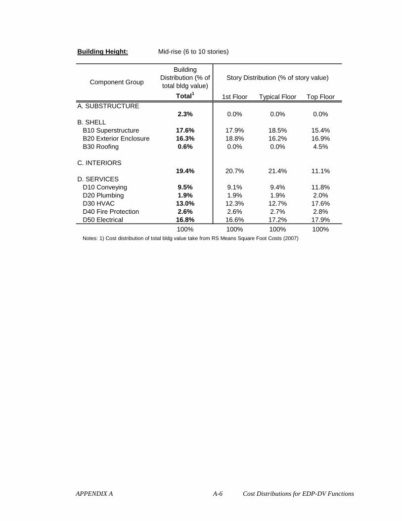
APPENDIX A A-6 Cost Distributions for EDP-DV Functions
Building Height: Mid-rise (6 to 10 stories)
Total1 1st Floor Typical Floor Top Floor
A. SUBSTRUCTURE2.3% 0.0% 0.0% 0.0%
B. SHELLB10 Superstructure 17.6% 17.9% 18.5% 15.4%B20 Exterior Enclosure 16.3% 18.8% 16.2% 16.9%B30 Roofing 0.6% 0.0% 0.0% 4.5%
C. INTERIORS19.4% 20.7% 21.4% 11.1%
D. SERVICESD10 Conveying 9.5% 9.1% 9.4% 11.8%D20 Plumbing 1.9% 1.9% 1.9% 2.0%D30 HVAC 13.0% 12.3% 12.7% 17.6%D40 Fire Protection 2.6% 2.6% 2.7% 2.8%D50 Electrical 16.8% 16.6% 17.2% 17.9%
100% 100% 100% 100%Notes: 1) Cost distribution of total bldg value take from RS Means Square Foot Costs (2007)
Building Distribution (% of total bldg value)
Component GroupStory Distribution (% of story value)

APPENDIX A A-7 Cost Distributions for EDP-DV Functions
Building Height: Mid-riseFloor Type: 1st Floor
Component Seismic Sensitivity Fragility Group
B. SHELLB10 Superstructure
Slab Rugged 7.9%Beam-column Assembly IDR Structural 7.0%Slab-column Assembly IDR Structural 3.1%
B20 Exterior EnclosureExterior Walls IDR Partitions 10.5%Exterior Windows IDR Windows 7.2%Exterior Doors IDR Partitions 1.1%
B30 RoofingRoof Coverings Rugged 0.0%Roof Openings Rugged 0.0%
C. INTERIORSPartitions with finishes IDR Partitions 3.3%Interior Doors IDR Partitions 1.7%Fittings IDR Generic-Drift 0.8%Stair Construction IDR Generic-Drift 2.3%Floor Finishes - 60% carpet IDR DS3 Partition-like 4.8%
30% vinyl composite tile Rugged 2.4%10% ceramic tile Rugged 0.8%
Ceiling Finishes PFA Ceilings 4.6%
D. SERVICESD10 Conveying
Elevators & Lifts IDR Generic-Drift 0.9%PFA Generic-Accl 8.2%
D20 PlumbingPlumbing Fixtures IDR DS3 Partition-like 0.8%
Rugged 1.1%D30 HVAC
Terminal & Package Units PFA Generic-Accl 9.2%IDR Generic-Drift 3.1%
Other HVAC Sys. & Equipment –D40 Fire Protection
Sprinklers PFA Generic-Accl 1.9%Standpipes IDR Generic-Drift 0.6%
D50 ElectricalElectrical Service/Distribution PFA Generic-Accl 1.5%Lighting & Branch Wiring Rugged 1.0%Lighting & Branch Wiring PFA Generic-Accl 5.0%Lighting & Branch Wiring IDR DS3 Partition-like 4.3%Communications & Security Rugged 1.0%Communications & Security PFA Generic-Accl 1.4%Communications & Security IDR DS3 Partition-like 2.4%
= 100% 100%
17.9%
Normalized costs
12.3%
16.6%
2.6%
1.9%
20.7%
9.1%
18.8%
0.0%

APPENDIX A A-8 Cost Distributions for EDP-DV Functions
Building Height: Mid-riseFloor Type: Typical Floor
Component Seismic Sensitivity Fragility Group
B. SHELLB10 Superstructure
Slab Rugged 8.2%Beam-column Assembly IDR Structural 7.2%Slab-column Assembly IDR Structural 3.1%
B20 Exterior EnclosureExterior Walls IDR Partitions 9.1%Exterior Windows IDR Windows 6.2%Exterior Doors IDR Partitions 1.0%
B30 RoofingRoof Coverings Rugged 0.0%Roof Openings Rugged 0.0%
C. INTERIORSPartitions with finishes IDR Partitions 4.5%Interior Doors IDR Partitions 1.9%Fittings IDR Generic-Drift 0.6%Stair Construction IDR Generic-Drift 1.9%Floor Finishes - 60% carpet IDR DS3 Partition-like 4.4%
30% vinyl composite tile Rugged 2.2%10% ceramic tile Rugged 0.7%
Ceiling Finishes PFA Ceilings 5.1%
D. SERVICESD10 Conveying
Elevators & Lifts IDR Generic-Drift 0.9%PFA Generic-Accl 8.5%
D20 PlumbingPlumbing Fixtures IDR DS3 Partition-like 0.9%
Rugged 1.1%D30 HVAC
Terminal & Package Units PFA Generic-Accl 9.5%IDR Generic-Drift 3.2%
Other HVAC Sys. & Equipment –D40 Fire Protection
Sprinklers PFA Generic-Accl 2.0%Standpipes IDR Generic-Drift 0.7%
D50 ElectricalElectrical Service/Distribution PFA Generic-Accl 1.5%Lighting & Branch Wiring Rugged 1.1%Lighting & Branch Wiring PFA Generic-Accl 5.1%Lighting & Branch Wiring IDR DS3 Partition-like 4.5%Communications & Security Rugged 1.0%Communications & Security PFA Generic-Accl 1.5%Communications & Security IDR DS3 Partition-like 2.5%
= 100% 100%
18.5%
17.2%
Normalized costs
9.4%
16.2%
0.0%
12.7%
2.7%
1.9%
21.4%

APPENDIX A A-9 Cost Distributions for EDP-DV Functions
Building Height: Mid-riseFloor Type: Top Floor
Component Seismic Sensitivity Fragility Group
B. SHELLB10 Superstructure
Slab Rugged 6.8%Beam-column Assembly IDR Structural 6.0%Slab-column Assembly IDR Structural 2.6%
B20 Exterior EnclosureExterior Walls IDR Partitions 9.5%Exterior Windows IDR Windows 6.4%Exterior Doors IDR Partitions 1.0%
B30 RoofingRoof Coverings Rugged 2.2%Roof Openings Rugged 2.2%
C. INTERIORSPartitions with finishes IDR Partitions 1.8%Interior Doors IDR Partitions 0.9%Fittings IDR Generic-Drift 0.4%Stair Construction IDR Generic-Drift 1.2%Floor Finishes - 60% carpet IDR DS3 Partition-like 2.6%
30% vinyl composite tile Rugged 1.3%10% ceramic tile Rugged 0.4%
Ceiling Finishes PFA Ceilings 2.4%
D. SERVICESD10 Conveying
Elevators & Lifts IDR Generic-Drift 1.2%PFA Generic-Accl 10.6%
D20 PlumbingPlumbing Fixtures IDR DS3 Partition-like 0.9%
Rugged 1.1%D30 HVAC
Terminal & Package Units PFA Generic-Accl 13.2%IDR Generic-Drift 4.4%
Other HVAC Sys. & Equipment PFA Generic-Accl 0.0%D40 Fire Protection
Sprinklers PFA Generic-Accl 2.1%Standpipes IDR Generic-Drift 0.7%
D50 ElectricalElectrical Service/Distribution PFA Generic-Accl 1.6%Lighting & Branch Wiring Rugged 1.1%Lighting & Branch Wiring PFA Generic-Accl 5.3%Lighting & Branch Wiring IDR DS3 Partition-like 4.7%Communications & Security Rugged 1.0%Communications & Security PFA Generic-Accl 1.6%Communications & Security IDR DS3 Partition-like 2.6%
= 100% 100%
15.4%
17.9%
2.8%
Normalized costs
17.6%
2.0%
11.1%
11.8%
16.9%
4.5%

APPENDIX A A-10 Cost Distributions for EDP-DV Functions
Building Height: High-rise (>10 stories)
Total1 1st Floor Typical Floor Top Floor
A. SUBSTRUCTURE1.5% 0.0% 0.0% 0.0%
B. SHELLB10 Superstructure 23.0% 23.1% 23.8% 19.8%B20 Exterior Enclosure 14.3% 16.6% 14.2% 14.9%B30 Roofing 0.3% 0.0% 0.0% 3.5%
C. INTERIORS17.1% 17.7% 18.2% 9.5%
D. SERVICESD10 Conveying 4.9% 4.7% 4.9% 6.1%D20 Plumbing 1.3% 1.3% 1.3% 1.4%D30 HVAC 16.6% 15.9% 16.3% 22.7%D40 Fire Protection 4.2% 4.1% 4.3% 4.4%D50 Electrical 16.8% 16.6% 17.0% 17.8%
100% 100% 100% 100%Notes: 1) Cost distribution of total bldg value take from RS Means Square Foot Costs (2007)
Building Distribution (% of total bldg value)
Component GroupStory Distribution (% of story value)

APPENDIX A A-11 Cost Distributions for EDP-DV Functions
Building Height: High-riseFloor Type: 1st Floor
Performance Group Seismic Sensitivity Fragility Group
B. SHELLB10 Superstructure
Slab Rugged 10.2%Beam-column Assembly IDR Structural 9.0%Slab-column Assembly IDR Structural 3.9%
B20 Exterior EnclosureExterior Walls IDR Partitions 9.3%Exterior Windows IDR Windows 6.3%Exterior Doors IDR Partitions 1.0%
B30 RoofingRoof Coverings Rugged 0.0%Roof Openings Rugged 0.0%
C. INTERIORSPartitions with finishes IDR Partitions 2.8%Interior Doors IDR Partitions 1.4%Fittings IDR Generic-Drift 0.7%Stair Construction IDR Generic-Drift 1.9%Floor Finishes - 60% carpet IDR DS3 Partition-like 4.1%
30% vinyl composite tile Rugged 2.1%10% ceramic tile Rugged 0.7%
Ceiling Finishes PFA Ceilings 3.9%
D. SERVICESD10 Conveying
Elevators & Lifts IDR Generic-Drift 0.5%PFA Generic-Accl 4.3%
D20 PlumbingPlumbing Fixtures IDR DS3 Partition-like 0.6%
Rugged 0.7%D30 HVAC
Terminal & Package Units PFA Generic-Accl 11.9%IDR Generic-Drift 4.0%
Other HVAC Sys. & Equipment –D40 Fire Protection
Sprinklers PFA Generic-Accl 3.1%Standpipes IDR Generic-Drift 1.0%
D50 ElectricalElectrical Service/Distribution PFA Generic-Accl 1.5%Lighting & Branch Wiring Rugged 1.0%Lighting & Branch Wiring PFA Generic-Accl 4.9%Lighting & Branch Wiring IDR DS3 Partition-like 4.3%Communications & Security Rugged 1.0%Communications & Security PFA Generic-Accl 1.4%Communications & Security IDR DS3 Partition-like 2.4%
= 100% 100%
Normalized costs
16.6%
4.1%
1.3%
15.9%
17.7%
4.7%
16.6%
0.0%
23.1%
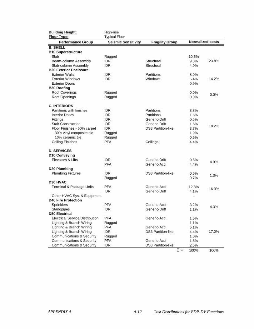
APPENDIX A A-12 Cost Distributions for EDP-DV Functions
Building Height: High-riseFloor Type: Typical Floor
Performance Group Seismic Sensitivity Fragility Group
B. SHELLB10 Superstructure
Slab Rugged 10.5%Beam-column Assembly IDR Structural 9.3%Slab-column Assembly IDR Structural 4.0%
B20 Exterior EnclosureExterior Walls IDR Partitions 8.0%Exterior Windows IDR Windows 5.4%Exterior Doors 0.9%
B30 RoofingRoof Coverings Rugged 0.0%Roof Openings Rugged 0.0%
C. INTERIORSPartitions with finishes IDR Partitions 3.8%Interior Doors IDR Partitions 1.6%Fittings IDR Generic-Drift 0.5%Stair Construction IDR Generic-Drift 1.6%Floor Finishes - 60% carpet IDR DS3 Partition-like 3.7%
30% vinyl composite tile Rugged 1.9%10% ceramic tile Rugged 0.6%
Ceiling Finishes PFA Ceilings 4.4%
D. SERVICESD10 Conveying
Elevators & Lifts IDR Generic-Drift 0.5%PFA Generic-Accl 4.4%
D20 PlumbingPlumbing Fixtures IDR DS3 Partition-like 0.6%
Rugged 0.7%D30 HVAC
Terminal & Package Units PFA Generic-Accl 12.3%IDR Generic-Drift 4.1%
Other HVAC Sys. & Equipment –D40 Fire Protection
Sprinklers PFA Generic-Accl 3.2%Standpipes IDR Generic-Drift 1.1%
D50 ElectricalElectrical Service/Distribution PFA Generic-Accl 1.5%Lighting & Branch Wiring Rugged 1.1%Lighting & Branch Wiring PFA Generic-Accl 5.1%Lighting & Branch Wiring IDR DS3 Partition-like 4.4%Communications & Security Rugged 1.0%Communications & Security PFA Generic-Accl 1.5%Communications & Security IDR DS3 Partition-like 2.5%
= 100% 100%
Normalized costs
23.8%
1.3%
17.0%
4.3%
16.3%
18.2%
4.9%
14.2%
0.0%

APPENDIX A A-13 Cost Distributions for EDP-DV Functions
Building Height: High-riseFloor Type: Top Floor
Performance Group Seismic Sensitivity Fragility Group
B. SHELLB10 Superstructure
Slab Rugged 8.7%Beam-column Assembly IDR Structural 7.7%Slab-column Assembly IDR Structural 3.4%
B20 Exterior EnclosureExterior Walls IDR Partitions 8.3%Exterior Windows IDR Windows 5.6%Exterior Doors IDR Partitions 0.9%
B30 RoofingRoof Coverings Rugged 1.7%Roof Openings Rugged 1.7%
C. INTERIORSPartitions with finishes IDR Partitions 1.5%Interior Doors IDR Partitions 0.8%Fittings IDR Generic-Drift 0.4%Stair Construction IDR Generic-Drift 1.0%Floor Finishes - 60% carpet IDR DS3 Partition-like 2.2%
30% vinyl composite tile Rugged 1.1%10% ceramic tile Rugged 0.4%
Ceiling Finishes PFA Ceilings 2.1%
D. SERVICESD10 Conveying
Elevators & Lifts IDR Generic-Drift 0.6%PFA Generic-Accl 5.5%
D20 PlumbingPlumbing Fixtures IDR DS3 Partition-like 0.6%
Rugged 0.8%D30 HVAC
Terminal & Package Units PFA Generic-Accl 17.0%IDR Generic-Drift 5.7%
Other HVAC Sys. & Equipment PFA Generic-Accl 0.0%D40 Fire Protection
Sprinklers PFA Generic-Accl 3.3%Standpipes IDR Generic-Drift 1.1%
D50 ElectricalElectrical Service/Distribution PFA Generic-Accl 1.6%Lighting & Branch Wiring Rugged 1.1%Lighting & Branch Wiring PFA Generic-Accl 5.3%Lighting & Branch Wiring IDR DS3 Partition-like 4.6%Communications & Security Rugged 1.0%Communications & Security PFA Generic-Accl 1.5%Communications & Security IDR DS3 Partition-like 2.6%
= 100% 100%
17.8%
4.4%
22.7%
Normalized costs
9.5%
19.8%
1.4%
6.1%
14.9%
3.5%
APPENDIX B B-1 Generic Story EDP-DV Functions
APPENDIX B
GENERIC STORY EDP-DV FUNCTIONS
This appendix contains the graphs and data points for the generic story EDP-DV
functions developed in Chapter 3. There are 36 functions for reinforced concrete moment-
resisting frame office buildings. On each sheet, a set of three functions for drift-sensitive
structural components, drift-sensitive nonstructural components and acceleration-sensitive
nonstructural components are reported. The sets of functions are categorized by the type of
frame four different building properties: the building height (low-rise, mid-rise or high-
rise), the type of material behavior (ductile or non-ductile reinforced concrete), the type of
structural frame (perimeter or space) and the location/type of floor (1st floor, typical floor or
top floor). The values of economic loss shown here are normalized by the replacement
value of the story. Interstory drift ratio (IDR) is unit-less and peak floor acceleration is
expressed in terms of the acceleration of gravity (g).

APPENDIX B B-2 Generic Story EDP-DV Functions
EDP-DV Function Data
Building Height: Low-rise (1 to 5 stories) IDR E(LS | IDR) IDR E(LNS | IDR) PFA E(LNS | PFA) IDR E(LS | IDR) IDR E(LNS | IDR) PFA E(LNS | PFA)
0.001 0.000 0.001 0.002 0.05 0.000 0.101 0.165 0.101 0.572 5.05 0.356
Strucutral Material: Ductile reinforced-concrete 0.002 0.000 0.002 0.009 0.10 0.000 0.102 0.166 0.102 0.572 5.10 0.3570.003 0.000 0.003 0.016 0.15 0.000 0.103 0.167 0.103 0.572 5.15 0.358
Structural System: Perimeter moment-frame 0.004 0.001 0.004 0.027 0.20 0.002 0.104 0.167 0.104 0.572 5.20 0.3580.005 0.002 0.005 0.044 0.25 0.004 0.105 0.168 0.105 0.573 5.25 0.359
Occupancy: Office 0.006 0.003 0.006 0.067 0.30 0.006 0.106 0.169 0.106 0.573 5.30 0.3600.007 0.006 0.007 0.094 0.35 0.009 0.107 0.170 0.107 0.573 5.35 0.361
Floor Type: 1st Floor 0.008 0.008 0.008 0.124 0.40 0.013 0.108 0.170 0.108 0.573 5.40 0.3610.009 0.011 0.009 0.154 0.45 0.016 0.109 0.171 0.109 0.573 5.45 0.3620.010 0.014 0.010 0.185 0.50 0.020 0.110 0.172 0.110 0.573 5.50 0.3630.011 0.017 0.011 0.213 0.55 0.024 0.111 0.172 0.111 0.573 5.55 0.3630.012 0.019 0.012 0.240 0.60 0.029 0.112 0.173 0.112 0.574 5.60 0.3640.013 0.021 0.013 0.265 0.65 0.034 0.113 0.173 0.113 0.574 5.65 0.3640.014 0.023 0.014 0.288 0.70 0.040 0.114 0.174 0.114 0.574 5.70 0.3650.015 0.024 0.015 0.308 0.75 0.045 0.115 0.174 0.115 0.574 5.75 0.3650.016 0.025 0.016 0.326 0.80 0.051 0.116 0.175 0.116 0.574 5.80 0.3660.017 0.026 0.017 0.342 0.85 0.057 0.117 0.175 0.117 0.574 5.85 0.3670.018 0.027 0.018 0.356 0.90 0.064 0.118 0.176 0.118 0.574 5.90 0.3670.019 0.028 0.019 0.369 0.95 0.070 0.119 0.176 0.119 0.574 5.95 0.3680.020 0.028 0.020 0.381 1.00 0.077 0.120 0.176 0.120 0.575 6.00 0.3680.021 0.029 0.021 0.391 1.05 0.084 0.121 0.177 0.121 0.575 6.05 0.3680.022 0.029 0.022 0.400 1.10 0.091 0.122 0.177 0.122 0.575 6.10 0.3690.023 0.030 0.023 0.409 1.15 0.098 0.123 0.178 0.123 0.575 6.15 0.3690.024 0.030 0.024 0.417 1.20 0.104 0.124 0.178 0.124 0.575 6.20 0.3700.025 0.030 0.025 0.425 1.25 0.111 0.125 0.178 0.125 0.575 6.25 0.3700.026 0.031 0.026 0.433 1.30 0.118 0.126 0.178 0.126 0.575 6.30 0.3710.027 0.031 0.027 0.440 1.35 0.125 0.127 0.179 0.127 0.575 6.35 0.3710.028 0.032 0.028 0.447 1.40 0.132 0.128 0.179 0.128 0.575 6.40 0.3710.029 0.032 0.029 0.453 1.45 0.138 0.129 0.179 0.129 0.575 6.45 0.3720.030 0.033 0.030 0.460 1.50 0.145 0.130 0.179 0.130 0.575 6.50 0.3720.031 0.033 0.031 0.466 1.55 0.151 0.131 0.180 0.131 0.575 6.55 0.3720.032 0.034 0.032 0.472 1.60 0.158 0.132 0.180 0.132 0.576 6.60 0.3730.033 0.034 0.033 0.478 1.65 0.164 0.133 0.180 0.133 0.576 6.65 0.3730.034 0.035 0.034 0.484 1.70 0.170 0.134 0.180 0.134 0.576 6.70 0.3730.035 0.035 0.035 0.489 1.75 0.176 0.135 0.180 0.135 0.576 6.75 0.3740.036 0.036 0.036 0.494 1.80 0.182 0.136 0.181 0.136 0.576 6.80 0.3740.037 0.037 0.037 0.499 1.85 0.188 0.137 0.181 0.137 0.576 6.85 0.3740.038 0.038 0.038 0.504 1.90 0.193 0.138 0.181 0.138 0.576 6.90 0.3750.039 0.039 0.039 0.508 1.95 0.199 0.139 0.181 0.139 0.576 6.95 0.3750.040 0.040 0.040 0.512 2.00 0.204 0.140 0.181 0.140 0.576 7.00 0.3750.041 0.041 0.041 0.516 2.05 0.209 0.141 0.181 0.141 0.576 7.05 0.3750.042 0.042 0.042 0.520 2.10 0.215 0.142 0.181 0.142 0.576 7.10 0.3760.043 0.044 0.043 0.523 2.15 0.220 0.143 0.181 0.143 0.576 7.15 0.3760.044 0.045 0.044 0.526 2.20 0.224 0.144 0.181 0.144 0.576 7.20 0.3760.045 0.047 0.045 0.529 2.25 0.229 0.145 0.182 0.145 0.576 7.25 0.3760.046 0.049 0.046 0.532 2.30 0.234 0.146 0.182 0.146 0.576 7.30 0.3770.047 0.051 0.047 0.534 2.35 0.238 0.147 0.182 0.147 0.576 7.35 0.3770.048 0.053 0.048 0.537 2.40 0.243 0.148 0.182 0.148 0.576 7.40 0.3770.049 0.056 0.049 0.539 2.45 0.247 0.149 0.182 0.149 0.577 7.45 0.3770.050 0.058 0.050 0.541 2.50 0.251 0.150 0.182 0.150 0.577 7.50 0.3770.051 0.061 0.051 0.543 2.55 0.255 0.151 0.182 0.151 0.577 7.55 0.3780.052 0.063 0.052 0.544 2.60 0.259 0.152 0.182 0.152 0.577 7.60 0.3780.053 0.066 0.053 0.546 2.65 0.263 0.153 0.182 0.153 0.577 7.65 0.3780.054 0.069 0.054 0.547 2.70 0.266 0.154 0.182 0.154 0.577 7.70 0.3780.055 0.072 0.055 0.549 2.75 0.270 0.155 0.182 0.155 0.577 7.75 0.3780.056 0.075 0.056 0.550 2.80 0.273 0.156 0.182 0.156 0.577 7.80 0.3790.057 0.078 0.057 0.551 2.85 0.277 0.157 0.182 0.157 0.577 7.85 0.3790.058 0.081 0.058 0.552 2.90 0.280 0.158 0.182 0.158 0.577 7.90 0.3790.059 0.084 0.059 0.553 2.95 0.283 0.159 0.182 0.159 0.577 7.95 0.3790.060 0.087 0.060 0.554 3.00 0.286 0.160 0.182 0.160 0.577 8.00 0.3790.061 0.090 0.061 0.555 3.05 0.289 0.161 0.182 0.161 0.577 8.05 0.3790.062 0.093 0.062 0.556 3.10 0.292 0.162 0.182 0.162 0.577 8.10 0.3790.063 0.096 0.063 0.557 3.15 0.295 0.163 0.182 0.163 0.577 8.15 0.3800.064 0.099 0.064 0.558 3.20 0.298 0.164 0.182 0.164 0.577 8.20 0.3800.065 0.102 0.065 0.559 3.25 0.300 0.165 0.183 0.165 0.577 8.25 0.3800.066 0.105 0.066 0.559 3.30 0.303 0.166 0.183 0.166 0.577 8.30 0.3800.067 0.107 0.067 0.560 3.35 0.305 0.167 0.183 0.167 0.577 8.35 0.3800.068 0.110 0.068 0.561 3.40 0.308 0.168 0.183 0.168 0.577 8.40 0.3800.069 0.113 0.069 0.561 3.45 0.310 0.169 0.183 0.169 0.577 8.45 0.3800.070 0.115 0.070 0.562 3.50 0.312 0.170 0.183 0.170 0.577 8.50 0.3810.071 0.118 0.071 0.562 3.55 0.314 0.171 0.183 0.171 0.577 8.55 0.3810.072 0.120 0.072 0.563 3.60 0.316 0.172 0.183 0.172 0.577 8.60 0.3810.073 0.123 0.073 0.563 3.65 0.319 0.173 0.183 0.173 0.577 8.65 0.3810.074 0.125 0.074 0.564 3.70 0.321 0.174 0.183 0.174 0.577 8.70 0.3810.075 0.127 0.075 0.564 3.75 0.322 0.175 0.183 0.175 0.577 8.75 0.3810.076 0.129 0.076 0.565 3.80 0.324 0.176 0.183 0.176 0.577 8.80 0.3810.077 0.131 0.077 0.565 3.85 0.326 0.177 0.183 0.177 0.577 8.85 0.3810.078 0.133 0.078 0.566 3.90 0.328 0.178 0.183 0.178 0.577 8.90 0.3810.079 0.135 0.079 0.566 3.95 0.330 0.179 0.183 0.179 0.577 8.95 0.3810.080 0.137 0.080 0.566 4.00 0.331 0.180 0.183 0.180 0.577 9.00 0.3820.081 0.139 0.081 0.567 4.05 0.333 0.181 0.183 0.181 0.577 9.05 0.3820.082 0.141 0.082 0.567 4.10 0.334 0.182 0.183 0.182 0.578 9.10 0.3820.083 0.142 0.083 0.567 4.15 0.336 0.183 0.183 0.183 0.578 9.15 0.3820.084 0.144 0.084 0.568 4.20 0.337 0.184 0.183 0.184 0.578 9.20 0.3820.085 0.146 0.085 0.568 4.25 0.339 0.185 0.183 0.185 0.578 9.25 0.3820.086 0.147 0.086 0.568 4.30 0.340 0.186 0.183 0.186 0.578 9.30 0.3820.087 0.149 0.087 0.569 4.35 0.341 0.187 0.183 0.187 0.578 9.35 0.3820.088 0.150 0.088 0.569 4.40 0.343 0.188 0.183 0.188 0.578 9.40 0.3820.089 0.151 0.089 0.569 4.45 0.344 0.189 0.183 0.189 0.578 9.45 0.3820.090 0.153 0.090 0.569 4.50 0.345 0.190 0.183 0.190 0.578 9.50 0.3820.091 0.154 0.091 0.570 4.55 0.346 0.191 0.183 0.191 0.578 9.55 0.3820.092 0.155 0.092 0.570 4.60 0.347 0.192 0.183 0.192 0.578 9.60 0.3820.093 0.157 0.093 0.570 4.65 0.348 0.193 0.183 0.193 0.578 9.65 0.3830.094 0.158 0.094 0.570 4.70 0.349 0.194 0.183 0.194 0.578 9.70 0.3830.095 0.159 0.095 0.571 4.75 0.350 0.195 0.183 0.195 0.578 9.75 0.3830.096 0.160 0.096 0.571 4.80 0.351 0.196 0.183 0.196 0.578 9.80 0.3830.097 0.161 0.097 0.571 4.85 0.352 0.197 0.183 0.197 0.578 9.85 0.3830.098 0.162 0.098 0.571 4.90 0.353 0.198 0.183 0.198 0.578 9.90 0.3830.099 0.163 0.099 0.571 4.95 0.354 0.199 0.183 0.199 0.578 9.95 0.3830.100 0.164 0.100 0.572 5.00 0.355 0.200 0.183 0.200 0.578 10.00 0.383
Loss Functions Loss Functions (cont'd)
Structural components
0.00
0.10
0.20
0.30
0.40
0.50
0.60
0.70
0.80
0.90
1.00
0.00 0.05 0.10 0.15 0.20IDR
E(L | IDR)
Nonstructural components
0.00
0.10
0.20
0.30
0.40
0.50
0.60
0.70
0.80
0.90
1.00
0.00 0.05 0.10 0.15 0.20IDR
E(L | IDR)
Nonstructural components
0.00
0.10
0.20
0.30
0.40
0.50
0.60
0.70
0.80
0.90
1.00
0.00 2.00 4.00 6.00 8.00 10.00PFA [g]
E(L | PFA)
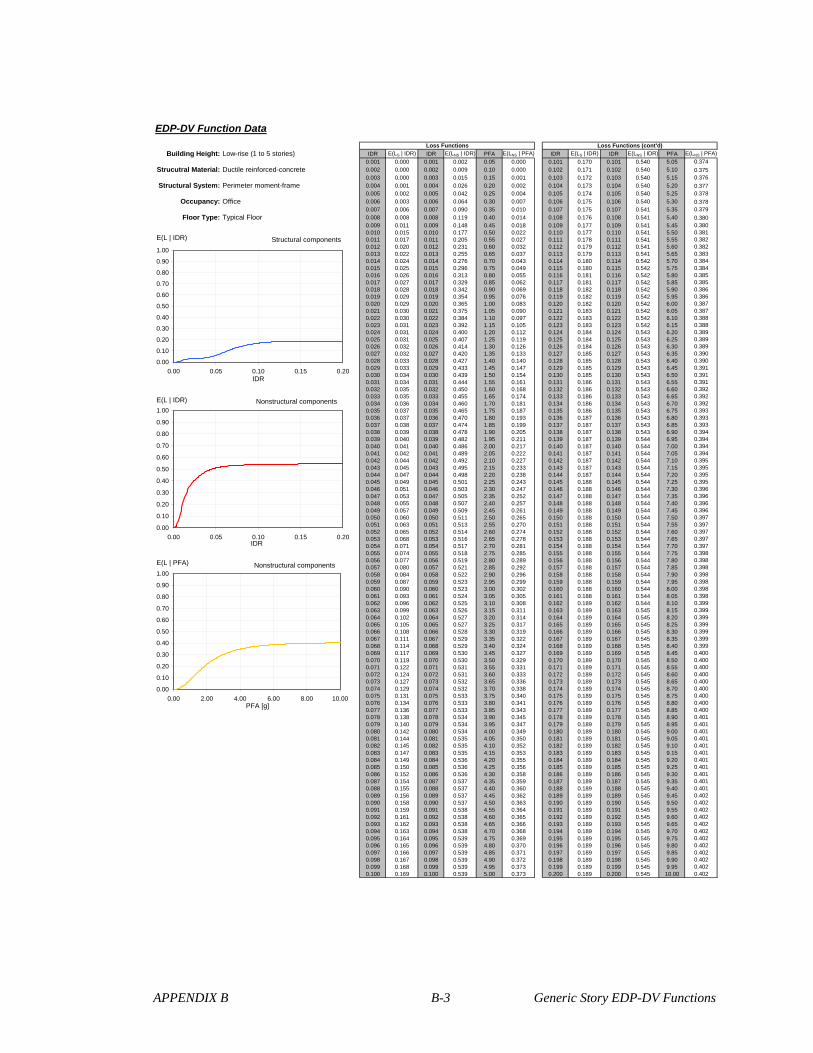
APPENDIX B B-3 Generic Story EDP-DV Functions
EDP-DV Function Data
Building Height: Low-rise (1 to 5 stories) IDR E(LS | IDR) IDR E(LNS | IDR) PFA E(LNS | PFA) IDR E(LS | IDR) IDR E(LNS | IDR) PFA E(LNS | PFA)
0.001 0.000 0.001 0.002 0.05 0.000 0.101 0.170 0.101 0.540 5.05 0.374
Strucutral Material: Ductile reinforced-concrete 0.002 0.000 0.002 0.009 0.10 0.000 0.102 0.171 0.102 0.540 5.10 0.3750.003 0.000 0.003 0.015 0.15 0.001 0.103 0.172 0.103 0.540 5.15 0.376
Structural System: Perimeter moment-frame 0.004 0.001 0.004 0.026 0.20 0.002 0.104 0.173 0.104 0.540 5.20 0.3770.005 0.002 0.005 0.042 0.25 0.004 0.105 0.174 0.105 0.540 5.25 0.378
Occupancy: Office 0.006 0.003 0.006 0.064 0.30 0.007 0.106 0.175 0.106 0.540 5.30 0.3780.007 0.006 0.007 0.090 0.35 0.010 0.107 0.175 0.107 0.541 5.35 0.379
Floor Type: Typical Floor 0.008 0.008 0.008 0.119 0.40 0.014 0.108 0.176 0.108 0.541 5.40 0.3800.009 0.011 0.009 0.148 0.45 0.018 0.109 0.177 0.109 0.541 5.45 0.3800.010 0.015 0.010 0.177 0.50 0.022 0.110 0.177 0.110 0.541 5.50 0.3810.011 0.017 0.011 0.205 0.55 0.027 0.111 0.178 0.111 0.541 5.55 0.3820.012 0.020 0.012 0.231 0.60 0.032 0.112 0.179 0.112 0.541 5.60 0.3820.013 0.022 0.013 0.255 0.65 0.037 0.113 0.179 0.113 0.541 5.65 0.3830.014 0.024 0.014 0.276 0.70 0.043 0.114 0.180 0.114 0.542 5.70 0.3840.015 0.025 0.015 0.296 0.75 0.049 0.115 0.180 0.115 0.542 5.75 0.3840.016 0.026 0.016 0.313 0.80 0.055 0.116 0.181 0.116 0.542 5.80 0.3850.017 0.027 0.017 0.329 0.85 0.062 0.117 0.181 0.117 0.542 5.85 0.3850.018 0.028 0.018 0.342 0.90 0.069 0.118 0.182 0.118 0.542 5.90 0.3860.019 0.029 0.019 0.354 0.95 0.076 0.119 0.182 0.119 0.542 5.95 0.3860.020 0.029 0.020 0.365 1.00 0.083 0.120 0.182 0.120 0.542 6.00 0.3870.021 0.030 0.021 0.375 1.05 0.090 0.121 0.183 0.121 0.542 6.05 0.3870.022 0.030 0.022 0.384 1.10 0.097 0.122 0.183 0.122 0.542 6.10 0.3880.023 0.031 0.023 0.392 1.15 0.105 0.123 0.183 0.123 0.542 6.15 0.3880.024 0.031 0.024 0.400 1.20 0.112 0.124 0.184 0.124 0.543 6.20 0.3890.025 0.031 0.025 0.407 1.25 0.119 0.125 0.184 0.125 0.543 6.25 0.3890.026 0.032 0.026 0.414 1.30 0.126 0.126 0.184 0.126 0.543 6.30 0.3890.027 0.032 0.027 0.420 1.35 0.133 0.127 0.185 0.127 0.543 6.35 0.3900.028 0.033 0.028 0.427 1.40 0.140 0.128 0.185 0.128 0.543 6.40 0.3900.029 0.033 0.029 0.433 1.45 0.147 0.129 0.185 0.129 0.543 6.45 0.3910.030 0.034 0.030 0.439 1.50 0.154 0.130 0.185 0.130 0.543 6.50 0.3910.031 0.034 0.031 0.444 1.55 0.161 0.131 0.186 0.131 0.543 6.55 0.3910.032 0.035 0.032 0.450 1.60 0.168 0.132 0.186 0.132 0.543 6.60 0.3920.033 0.035 0.033 0.455 1.65 0.174 0.133 0.186 0.133 0.543 6.65 0.3920.034 0.036 0.034 0.460 1.70 0.181 0.134 0.186 0.134 0.543 6.70 0.3920.035 0.037 0.035 0.465 1.75 0.187 0.135 0.186 0.135 0.543 6.75 0.3930.036 0.037 0.036 0.470 1.80 0.193 0.136 0.187 0.136 0.543 6.80 0.3930.037 0.038 0.037 0.474 1.85 0.199 0.137 0.187 0.137 0.543 6.85 0.3930.038 0.039 0.038 0.478 1.90 0.205 0.138 0.187 0.138 0.543 6.90 0.3940.039 0.040 0.039 0.482 1.95 0.211 0.139 0.187 0.139 0.544 6.95 0.3940.040 0.041 0.040 0.486 2.00 0.217 0.140 0.187 0.140 0.544 7.00 0.3940.041 0.042 0.041 0.489 2.05 0.222 0.141 0.187 0.141 0.544 7.05 0.3940.042 0.044 0.042 0.492 2.10 0.227 0.142 0.187 0.142 0.544 7.10 0.3950.043 0.045 0.043 0.495 2.15 0.233 0.143 0.187 0.143 0.544 7.15 0.3950.044 0.047 0.044 0.498 2.20 0.238 0.144 0.187 0.144 0.544 7.20 0.3950.045 0.049 0.045 0.501 2.25 0.243 0.145 0.188 0.145 0.544 7.25 0.3950.046 0.051 0.046 0.503 2.30 0.247 0.146 0.188 0.146 0.544 7.30 0.3960.047 0.053 0.047 0.505 2.35 0.252 0.147 0.188 0.147 0.544 7.35 0.3960.048 0.055 0.048 0.507 2.40 0.257 0.148 0.188 0.148 0.544 7.40 0.3960.049 0.057 0.049 0.509 2.45 0.261 0.149 0.188 0.149 0.544 7.45 0.3960.050 0.060 0.050 0.511 2.50 0.265 0.150 0.188 0.150 0.544 7.50 0.3970.051 0.063 0.051 0.513 2.55 0.270 0.151 0.188 0.151 0.544 7.55 0.3970.052 0.065 0.052 0.514 2.60 0.274 0.152 0.188 0.152 0.544 7.60 0.3970.053 0.068 0.053 0.516 2.65 0.278 0.153 0.188 0.153 0.544 7.65 0.3970.054 0.071 0.054 0.517 2.70 0.281 0.154 0.188 0.154 0.544 7.70 0.3970.055 0.074 0.055 0.518 2.75 0.285 0.155 0.188 0.155 0.544 7.75 0.3980.056 0.077 0.056 0.519 2.80 0.289 0.156 0.188 0.156 0.544 7.80 0.3980.057 0.080 0.057 0.521 2.85 0.292 0.157 0.188 0.157 0.544 7.85 0.3980.058 0.084 0.058 0.522 2.90 0.296 0.158 0.188 0.158 0.544 7.90 0.3980.059 0.087 0.059 0.523 2.95 0.299 0.159 0.188 0.159 0.544 7.95 0.3980.060 0.090 0.060 0.523 3.00 0.302 0.160 0.188 0.160 0.544 8.00 0.3980.061 0.093 0.061 0.524 3.05 0.305 0.161 0.188 0.161 0.544 8.05 0.3980.062 0.096 0.062 0.525 3.10 0.308 0.162 0.189 0.162 0.544 8.10 0.3990.063 0.099 0.063 0.526 3.15 0.311 0.163 0.189 0.163 0.545 8.15 0.3990.064 0.102 0.064 0.527 3.20 0.314 0.164 0.189 0.164 0.545 8.20 0.3990.065 0.105 0.065 0.527 3.25 0.317 0.165 0.189 0.165 0.545 8.25 0.3990.066 0.108 0.066 0.528 3.30 0.319 0.166 0.189 0.166 0.545 8.30 0.3990.067 0.111 0.067 0.529 3.35 0.322 0.167 0.189 0.167 0.545 8.35 0.3990.068 0.114 0.068 0.529 3.40 0.324 0.168 0.189 0.168 0.545 8.40 0.3990.069 0.117 0.069 0.530 3.45 0.327 0.169 0.189 0.169 0.545 8.45 0.4000.070 0.119 0.070 0.530 3.50 0.329 0.170 0.189 0.170 0.545 8.50 0.4000.071 0.122 0.071 0.531 3.55 0.331 0.171 0.189 0.171 0.545 8.55 0.4000.072 0.124 0.072 0.531 3.60 0.333 0.172 0.189 0.172 0.545 8.60 0.4000.073 0.127 0.073 0.532 3.65 0.336 0.173 0.189 0.173 0.545 8.65 0.4000.074 0.129 0.074 0.532 3.70 0.338 0.174 0.189 0.174 0.545 8.70 0.4000.075 0.131 0.075 0.533 3.75 0.340 0.175 0.189 0.175 0.545 8.75 0.4000.076 0.134 0.076 0.533 3.80 0.341 0.176 0.189 0.176 0.545 8.80 0.4000.077 0.136 0.077 0.533 3.85 0.343 0.177 0.189 0.177 0.545 8.85 0.4000.078 0.138 0.078 0.534 3.90 0.345 0.178 0.189 0.178 0.545 8.90 0.4010.079 0.140 0.079 0.534 3.95 0.347 0.179 0.189 0.179 0.545 8.95 0.4010.080 0.142 0.080 0.534 4.00 0.349 0.180 0.189 0.180 0.545 9.00 0.4010.081 0.144 0.081 0.535 4.05 0.350 0.181 0.189 0.181 0.545 9.05 0.4010.082 0.145 0.082 0.535 4.10 0.352 0.182 0.189 0.182 0.545 9.10 0.4010.083 0.147 0.083 0.535 4.15 0.353 0.183 0.189 0.183 0.545 9.15 0.4010.084 0.149 0.084 0.536 4.20 0.355 0.184 0.189 0.184 0.545 9.20 0.4010.085 0.150 0.085 0.536 4.25 0.356 0.185 0.189 0.185 0.545 9.25 0.4010.086 0.152 0.086 0.536 4.30 0.358 0.186 0.189 0.186 0.545 9.30 0.4010.087 0.154 0.087 0.537 4.35 0.359 0.187 0.189 0.187 0.545 9.35 0.4010.088 0.155 0.088 0.537 4.40 0.360 0.188 0.189 0.188 0.545 9.40 0.4010.089 0.156 0.089 0.537 4.45 0.362 0.189 0.189 0.189 0.545 9.45 0.4020.090 0.158 0.090 0.537 4.50 0.363 0.190 0.189 0.190 0.545 9.50 0.4020.091 0.159 0.091 0.538 4.55 0.364 0.191 0.189 0.191 0.545 9.55 0.4020.092 0.161 0.092 0.538 4.60 0.365 0.192 0.189 0.192 0.545 9.60 0.4020.093 0.162 0.093 0.538 4.65 0.366 0.193 0.189 0.193 0.545 9.65 0.4020.094 0.163 0.094 0.538 4.70 0.368 0.194 0.189 0.194 0.545 9.70 0.4020.095 0.164 0.095 0.539 4.75 0.369 0.195 0.189 0.195 0.545 9.75 0.4020.096 0.165 0.096 0.539 4.80 0.370 0.196 0.189 0.196 0.545 9.80 0.4020.097 0.166 0.097 0.539 4.85 0.371 0.197 0.189 0.197 0.545 9.85 0.4020.098 0.167 0.098 0.539 4.90 0.372 0.198 0.189 0.198 0.545 9.90 0.4020.099 0.168 0.099 0.539 4.95 0.373 0.199 0.189 0.199 0.545 9.95 0.4020.100 0.169 0.100 0.539 5.00 0.373 0.200 0.189 0.200 0.545 10.00 0.402
Loss Functions Loss Functions (cont'd)
Structural components
0.00
0.10
0.20
0.30
0.40
0.50
0.60
0.70
0.80
0.90
1.00
0.00 0.05 0.10 0.15 0.20IDR
E(L | IDR)
Nonstructural components
0.00
0.10
0.20
0.30
0.40
0.50
0.60
0.70
0.80
0.90
1.00
0.00 0.05 0.10 0.15 0.20IDR
E(L | IDR)
Nonstructural components
0.00
0.10
0.20
0.30
0.40
0.50
0.60
0.70
0.80
0.90
1.00
0.00 2.00 4.00 6.00 8.00 10.00PFA [g]
E(L | PFA)

APPENDIX B B-4 Generic Story EDP-DV Functions
EDP-DV Function Data
Building Height: Low-rise (1 to 5 stories) IDR E(LS | IDR) IDR E(LNS | IDR) PFA E(LNS | PFA) IDR E(LS | IDR) IDR E(LNS | IDR) PFA E(LNS | PFA)
0.001 0.000 0.001 0.002 0.05 0.000 0.101 0.140 0.101 0.478 5.05 0.397
Strucutral Material: Ductile reinforced-concrete 0.002 0.000 0.002 0.007 0.10 0.000 0.102 0.141 0.102 0.479 5.10 0.3980.003 0.000 0.003 0.013 0.15 0.000 0.103 0.142 0.103 0.479 5.15 0.399
Structural System: Perimeter moment-frame 0.004 0.001 0.004 0.021 0.20 0.001 0.104 0.142 0.104 0.479 5.20 0.4000.005 0.001 0.005 0.034 0.25 0.003 0.105 0.143 0.105 0.479 5.25 0.401
Occupancy: Office 0.006 0.003 0.006 0.052 0.30 0.005 0.106 0.144 0.106 0.479 5.30 0.4020.007 0.005 0.007 0.074 0.35 0.007 0.107 0.144 0.107 0.479 5.35 0.403
Floor Type: Top Floor 0.008 0.007 0.008 0.097 0.40 0.010 0.108 0.145 0.108 0.480 5.40 0.4040.009 0.009 0.009 0.122 0.45 0.013 0.109 0.145 0.109 0.480 5.45 0.4040.010 0.012 0.010 0.146 0.50 0.016 0.110 0.146 0.110 0.480 5.50 0.4050.011 0.014 0.011 0.169 0.55 0.020 0.111 0.146 0.111 0.480 5.55 0.4060.012 0.016 0.012 0.191 0.60 0.024 0.112 0.147 0.112 0.480 5.60 0.4070.013 0.018 0.013 0.211 0.65 0.029 0.113 0.147 0.113 0.480 5.65 0.4070.014 0.019 0.014 0.230 0.70 0.034 0.114 0.148 0.114 0.480 5.70 0.4080.015 0.021 0.015 0.246 0.75 0.040 0.115 0.148 0.115 0.480 5.75 0.4090.016 0.021 0.016 0.261 0.80 0.046 0.116 0.149 0.116 0.481 5.80 0.4100.017 0.022 0.017 0.275 0.85 0.052 0.117 0.149 0.117 0.481 5.85 0.4100.018 0.023 0.018 0.287 0.90 0.059 0.118 0.149 0.118 0.481 5.90 0.4110.019 0.023 0.019 0.297 0.95 0.065 0.119 0.150 0.119 0.481 5.95 0.4110.020 0.024 0.020 0.307 1.00 0.072 0.120 0.150 0.120 0.481 6.00 0.4120.021 0.024 0.021 0.315 1.05 0.079 0.121 0.150 0.121 0.481 6.05 0.4130.022 0.025 0.022 0.324 1.10 0.086 0.122 0.151 0.122 0.481 6.10 0.4130.023 0.025 0.023 0.331 1.15 0.094 0.123 0.151 0.123 0.481 6.15 0.4140.024 0.026 0.024 0.338 1.20 0.101 0.124 0.151 0.124 0.481 6.20 0.4140.025 0.026 0.025 0.345 1.25 0.109 0.125 0.151 0.125 0.481 6.25 0.4150.026 0.026 0.026 0.351 1.30 0.116 0.126 0.152 0.126 0.482 6.30 0.4150.027 0.027 0.027 0.358 1.35 0.123 0.127 0.152 0.127 0.482 6.35 0.4160.028 0.027 0.028 0.364 1.40 0.131 0.128 0.152 0.128 0.482 6.40 0.4160.029 0.027 0.029 0.370 1.45 0.138 0.129 0.152 0.129 0.482 6.45 0.4170.030 0.028 0.030 0.376 1.50 0.146 0.130 0.152 0.130 0.482 6.50 0.4170.031 0.028 0.031 0.381 1.55 0.153 0.131 0.153 0.131 0.482 6.55 0.4180.032 0.029 0.032 0.387 1.60 0.160 0.132 0.153 0.132 0.482 6.60 0.4180.033 0.029 0.033 0.392 1.65 0.167 0.133 0.153 0.133 0.482 6.65 0.4180.034 0.030 0.034 0.397 1.70 0.174 0.134 0.153 0.134 0.482 6.70 0.4190.035 0.030 0.035 0.402 1.75 0.181 0.135 0.153 0.135 0.482 6.75 0.4190.036 0.031 0.036 0.406 1.80 0.188 0.136 0.153 0.136 0.482 6.80 0.4200.037 0.031 0.037 0.411 1.85 0.194 0.137 0.154 0.137 0.482 6.85 0.4200.038 0.032 0.038 0.415 1.90 0.201 0.138 0.154 0.138 0.482 6.90 0.4200.039 0.033 0.039 0.419 1.95 0.207 0.139 0.154 0.139 0.482 6.95 0.4210.040 0.034 0.040 0.423 2.00 0.214 0.140 0.154 0.140 0.483 7.00 0.4210.041 0.035 0.041 0.426 2.05 0.220 0.141 0.154 0.141 0.483 7.05 0.4210.042 0.036 0.042 0.429 2.10 0.226 0.142 0.154 0.142 0.483 7.10 0.4220.043 0.037 0.043 0.432 2.15 0.232 0.143 0.154 0.143 0.483 7.15 0.4220.044 0.039 0.044 0.435 2.20 0.237 0.144 0.154 0.144 0.483 7.20 0.4220.045 0.040 0.045 0.438 2.25 0.243 0.145 0.154 0.145 0.483 7.25 0.4220.046 0.042 0.046 0.440 2.30 0.248 0.146 0.154 0.146 0.483 7.30 0.4230.047 0.043 0.047 0.443 2.35 0.254 0.147 0.154 0.147 0.483 7.35 0.4230.048 0.045 0.048 0.445 2.40 0.259 0.148 0.154 0.148 0.483 7.40 0.4230.049 0.047 0.049 0.447 2.45 0.264 0.149 0.155 0.149 0.483 7.45 0.4240.050 0.049 0.050 0.449 2.50 0.269 0.150 0.155 0.150 0.483 7.50 0.4240.051 0.051 0.051 0.450 2.55 0.274 0.151 0.155 0.151 0.483 7.55 0.4240.052 0.054 0.052 0.452 2.60 0.278 0.152 0.155 0.152 0.483 7.60 0.4240.053 0.056 0.053 0.454 2.65 0.283 0.153 0.155 0.153 0.483 7.65 0.4250.054 0.059 0.054 0.455 2.70 0.287 0.154 0.155 0.154 0.483 7.70 0.4250.055 0.061 0.055 0.456 2.75 0.292 0.155 0.155 0.155 0.483 7.75 0.4250.056 0.064 0.056 0.457 2.80 0.296 0.156 0.155 0.156 0.483 7.80 0.4250.057 0.066 0.057 0.459 2.85 0.300 0.157 0.155 0.157 0.483 7.85 0.4250.058 0.069 0.058 0.460 2.90 0.304 0.158 0.155 0.158 0.483 7.90 0.4260.059 0.071 0.059 0.461 2.95 0.308 0.159 0.155 0.159 0.483 7.95 0.4260.060 0.074 0.060 0.462 3.00 0.311 0.160 0.155 0.160 0.483 8.00 0.4260.061 0.077 0.061 0.462 3.05 0.315 0.161 0.155 0.161 0.483 8.05 0.4260.062 0.079 0.062 0.463 3.10 0.318 0.162 0.155 0.162 0.483 8.10 0.4260.063 0.082 0.063 0.464 3.15 0.322 0.163 0.155 0.163 0.483 8.15 0.4270.064 0.084 0.064 0.465 3.20 0.325 0.164 0.155 0.164 0.484 8.20 0.4270.065 0.087 0.065 0.466 3.25 0.328 0.165 0.155 0.165 0.484 8.25 0.4270.066 0.089 0.066 0.466 3.30 0.331 0.166 0.155 0.166 0.484 8.30 0.4270.067 0.091 0.067 0.467 3.35 0.334 0.167 0.155 0.167 0.484 8.35 0.4270.068 0.094 0.068 0.467 3.40 0.337 0.168 0.155 0.168 0.484 8.40 0.4270.069 0.096 0.069 0.468 3.45 0.340 0.169 0.155 0.169 0.484 8.45 0.4280.070 0.098 0.070 0.469 3.50 0.343 0.170 0.155 0.170 0.484 8.50 0.4280.071 0.100 0.071 0.469 3.55 0.346 0.171 0.155 0.171 0.484 8.55 0.4280.072 0.102 0.072 0.470 3.60 0.348 0.172 0.155 0.172 0.484 8.60 0.4280.073 0.104 0.073 0.470 3.65 0.351 0.173 0.155 0.173 0.484 8.65 0.4280.074 0.106 0.074 0.471 3.70 0.353 0.174 0.155 0.174 0.484 8.70 0.4280.075 0.108 0.075 0.471 3.75 0.356 0.175 0.155 0.175 0.484 8.75 0.4280.076 0.110 0.076 0.471 3.80 0.358 0.176 0.155 0.176 0.484 8.80 0.4280.077 0.112 0.077 0.472 3.85 0.360 0.177 0.155 0.177 0.484 8.85 0.4290.078 0.113 0.078 0.472 3.90 0.362 0.178 0.155 0.178 0.484 8.90 0.4290.079 0.115 0.079 0.473 3.95 0.364 0.179 0.155 0.179 0.484 8.95 0.4290.080 0.116 0.080 0.473 4.00 0.366 0.180 0.155 0.180 0.484 9.00 0.4290.081 0.118 0.081 0.473 4.05 0.368 0.181 0.155 0.181 0.484 9.05 0.4290.082 0.120 0.082 0.474 4.10 0.370 0.182 0.155 0.182 0.484 9.10 0.4290.083 0.121 0.083 0.474 4.15 0.372 0.183 0.155 0.183 0.484 9.15 0.4290.084 0.122 0.084 0.474 4.20 0.374 0.184 0.155 0.184 0.484 9.20 0.4290.085 0.124 0.085 0.475 4.25 0.376 0.185 0.155 0.185 0.484 9.25 0.4290.086 0.125 0.086 0.475 4.30 0.377 0.186 0.155 0.186 0.484 9.30 0.4300.087 0.126 0.087 0.475 4.35 0.379 0.187 0.155 0.187 0.484 9.35 0.4300.088 0.127 0.088 0.476 4.40 0.380 0.188 0.155 0.188 0.484 9.40 0.4300.089 0.129 0.089 0.476 4.45 0.382 0.189 0.155 0.189 0.484 9.45 0.4300.090 0.130 0.090 0.476 4.50 0.383 0.190 0.155 0.190 0.484 9.50 0.4300.091 0.131 0.091 0.476 4.55 0.385 0.191 0.155 0.191 0.484 9.55 0.4300.092 0.132 0.092 0.477 4.60 0.386 0.192 0.155 0.192 0.484 9.60 0.4300.093 0.133 0.093 0.477 4.65 0.388 0.193 0.155 0.193 0.484 9.65 0.4300.094 0.134 0.094 0.477 4.70 0.389 0.194 0.155 0.194 0.484 9.70 0.4300.095 0.135 0.095 0.477 4.75 0.390 0.195 0.155 0.195 0.484 9.75 0.4300.096 0.136 0.096 0.477 4.80 0.391 0.196 0.155 0.196 0.484 9.80 0.4300.097 0.137 0.097 0.478 4.85 0.393 0.197 0.155 0.197 0.484 9.85 0.4310.098 0.138 0.098 0.478 4.90 0.394 0.198 0.155 0.198 0.484 9.90 0.4310.099 0.139 0.099 0.478 4.95 0.395 0.199 0.155 0.199 0.484 9.95 0.4310.100 0.139 0.100 0.478 5.00 0.396 0.200 0.155 0.200 0.484 10.00 0.431
Loss Functions Loss Functions (cont'd)
Structural components
0.00
0.10
0.20
0.30
0.40
0.50
0.60
0.70
0.80
0.90
1.00
0.00 0.05 0.10 0.15 0.20IDR
E(L | IDR)
Nonstructural components
0.00
0.10
0.20
0.30
0.40
0.50
0.60
0.70
0.80
0.90
1.00
0.00 0.05 0.10 0.15 0.20IDR
E(L | IDR)
Nonstructural components
0.00
0.10
0.20
0.30
0.40
0.50
0.60
0.70
0.80
0.90
1.00
0.00 2.00 4.00 6.00 8.00 10.00PFA [g]
E(L | PFA)

APPENDIX B B-5 Generic Story EDP-DV Functions
EDP-DV Function Data
Building Height: Mid-rise (5 to 10 stories) IDR E(LS | IDR) IDR E(LNS | IDR) PFA E(LNS | PFA) IDR E(LS | IDR) IDR E(LNS | IDR) PFA E(LNS | PFA)
0.001 0.000 0.001 0.002 0.05 0.000 0.101 0.240 0.101 0.521 5.05 0.352
Strucutral Material: Ductile reinforced-concrete 0.002 0.000 0.002 0.008 0.10 0.000 0.102 0.242 0.102 0.522 5.10 0.3520.003 0.000 0.003 0.015 0.15 0.000 0.103 0.243 0.103 0.522 5.15 0.353
Structural System: Perimeter moment-frame 0.004 0.001 0.004 0.024 0.20 0.002 0.104 0.244 0.104 0.522 5.20 0.3540.005 0.003 0.005 0.040 0.25 0.003 0.105 0.245 0.105 0.522 5.25 0.355
Occupancy: Office 0.006 0.005 0.006 0.060 0.30 0.006 0.106 0.246 0.106 0.522 5.30 0.3560.007 0.008 0.007 0.085 0.35 0.008 0.107 0.247 0.107 0.522 5.35 0.356
Floor Type: 1st Floor 0.008 0.012 0.008 0.112 0.40 0.011 0.108 0.248 0.108 0.522 5.40 0.3570.009 0.016 0.009 0.139 0.45 0.014 0.109 0.249 0.109 0.523 5.45 0.3580.010 0.020 0.010 0.166 0.50 0.018 0.110 0.250 0.110 0.523 5.50 0.3580.011 0.024 0.011 0.192 0.55 0.022 0.111 0.251 0.111 0.523 5.55 0.3590.012 0.028 0.012 0.216 0.60 0.026 0.112 0.252 0.112 0.523 5.60 0.3600.013 0.031 0.013 0.238 0.65 0.031 0.113 0.253 0.113 0.523 5.65 0.3600.014 0.033 0.014 0.258 0.70 0.036 0.114 0.253 0.114 0.523 5.70 0.3610.015 0.035 0.015 0.277 0.75 0.041 0.115 0.254 0.115 0.523 5.75 0.3610.016 0.037 0.016 0.293 0.80 0.047 0.116 0.255 0.116 0.523 5.80 0.3620.017 0.038 0.017 0.307 0.85 0.053 0.117 0.255 0.117 0.524 5.85 0.3620.018 0.039 0.018 0.320 0.90 0.059 0.118 0.256 0.118 0.524 5.90 0.3630.019 0.040 0.019 0.331 0.95 0.065 0.119 0.257 0.119 0.524 5.95 0.3640.020 0.041 0.020 0.342 1.00 0.071 0.120 0.257 0.120 0.524 6.00 0.3640.021 0.042 0.021 0.351 1.05 0.078 0.121 0.258 0.121 0.524 6.05 0.3640.022 0.043 0.022 0.360 1.10 0.084 0.122 0.258 0.122 0.524 6.10 0.3650.023 0.043 0.023 0.368 1.15 0.091 0.123 0.259 0.123 0.524 6.15 0.3650.024 0.044 0.024 0.375 1.20 0.098 0.124 0.259 0.124 0.524 6.20 0.3660.025 0.044 0.025 0.383 1.25 0.104 0.125 0.260 0.125 0.524 6.25 0.3660.026 0.045 0.026 0.389 1.30 0.111 0.126 0.260 0.126 0.524 6.30 0.3670.027 0.046 0.027 0.396 1.35 0.118 0.127 0.260 0.127 0.524 6.35 0.3670.028 0.046 0.028 0.403 1.40 0.124 0.128 0.261 0.128 0.525 6.40 0.3670.029 0.047 0.029 0.409 1.45 0.131 0.129 0.261 0.129 0.525 6.45 0.3680.030 0.048 0.030 0.415 1.50 0.137 0.130 0.261 0.130 0.525 6.50 0.3680.031 0.048 0.031 0.421 1.55 0.144 0.131 0.262 0.131 0.525 6.55 0.3690.032 0.049 0.032 0.427 1.60 0.150 0.132 0.262 0.132 0.525 6.60 0.3690.033 0.050 0.033 0.432 1.65 0.156 0.133 0.262 0.133 0.525 6.65 0.3690.034 0.051 0.034 0.438 1.70 0.162 0.134 0.263 0.134 0.525 6.70 0.3700.035 0.052 0.035 0.443 1.75 0.168 0.135 0.263 0.135 0.525 6.75 0.3700.036 0.053 0.036 0.448 1.80 0.174 0.136 0.263 0.136 0.525 6.80 0.3700.037 0.054 0.037 0.452 1.85 0.180 0.137 0.263 0.137 0.525 6.85 0.3710.038 0.055 0.038 0.457 1.90 0.186 0.138 0.263 0.138 0.525 6.90 0.3710.039 0.056 0.039 0.461 1.95 0.191 0.139 0.264 0.139 0.525 6.95 0.3710.040 0.058 0.040 0.465 2.00 0.197 0.140 0.264 0.140 0.525 7.00 0.3710.041 0.060 0.041 0.469 2.05 0.202 0.141 0.264 0.141 0.525 7.05 0.3720.042 0.062 0.042 0.472 2.10 0.207 0.142 0.264 0.142 0.525 7.10 0.3720.043 0.064 0.043 0.475 2.15 0.212 0.143 0.264 0.143 0.525 7.15 0.3720.044 0.066 0.044 0.478 2.20 0.217 0.144 0.264 0.144 0.525 7.20 0.3720.045 0.069 0.045 0.481 2.25 0.222 0.145 0.265 0.145 0.526 7.25 0.3730.046 0.071 0.046 0.484 2.30 0.227 0.146 0.265 0.146 0.526 7.30 0.3730.047 0.074 0.047 0.486 2.35 0.231 0.147 0.265 0.147 0.526 7.35 0.3730.048 0.078 0.048 0.488 2.40 0.236 0.148 0.265 0.148 0.526 7.40 0.3730.049 0.081 0.049 0.490 2.45 0.240 0.149 0.265 0.149 0.526 7.45 0.3740.050 0.084 0.050 0.492 2.50 0.244 0.150 0.265 0.150 0.526 7.50 0.3740.051 0.088 0.051 0.494 2.55 0.248 0.151 0.265 0.151 0.526 7.55 0.3740.052 0.092 0.052 0.495 2.60 0.252 0.152 0.265 0.152 0.526 7.60 0.3740.053 0.096 0.053 0.497 2.65 0.256 0.153 0.265 0.153 0.526 7.65 0.3740.054 0.100 0.054 0.498 2.70 0.260 0.154 0.265 0.154 0.526 7.70 0.3750.055 0.105 0.055 0.500 2.75 0.263 0.155 0.266 0.155 0.526 7.75 0.3750.056 0.109 0.056 0.501 2.80 0.267 0.156 0.266 0.156 0.526 7.80 0.3750.057 0.113 0.057 0.502 2.85 0.270 0.157 0.266 0.157 0.526 7.85 0.3750.058 0.118 0.058 0.503 2.90 0.274 0.158 0.266 0.158 0.526 7.90 0.3750.059 0.122 0.059 0.504 2.95 0.277 0.159 0.266 0.159 0.526 7.95 0.3750.060 0.127 0.060 0.505 3.00 0.280 0.160 0.266 0.160 0.526 8.00 0.3760.061 0.131 0.061 0.506 3.05 0.283 0.161 0.266 0.161 0.526 8.05 0.3760.062 0.136 0.062 0.507 3.10 0.286 0.162 0.266 0.162 0.526 8.10 0.3760.063 0.140 0.063 0.508 3.15 0.289 0.163 0.266 0.163 0.526 8.15 0.3760.064 0.144 0.064 0.508 3.20 0.292 0.164 0.266 0.164 0.526 8.20 0.3760.065 0.148 0.065 0.509 3.25 0.294 0.165 0.266 0.165 0.526 8.25 0.3760.066 0.153 0.066 0.510 3.30 0.297 0.166 0.266 0.166 0.526 8.30 0.3760.067 0.157 0.067 0.510 3.35 0.299 0.167 0.266 0.167 0.526 8.35 0.3770.068 0.161 0.068 0.511 3.40 0.302 0.168 0.266 0.168 0.526 8.40 0.3770.069 0.164 0.069 0.511 3.45 0.304 0.169 0.266 0.169 0.526 8.45 0.3770.070 0.168 0.070 0.512 3.50 0.307 0.170 0.266 0.170 0.526 8.50 0.3770.071 0.172 0.071 0.512 3.55 0.309 0.171 0.266 0.171 0.526 8.55 0.3770.072 0.175 0.072 0.513 3.60 0.311 0.172 0.266 0.172 0.526 8.60 0.3770.073 0.179 0.073 0.513 3.65 0.313 0.173 0.266 0.173 0.526 8.65 0.3770.074 0.182 0.074 0.514 3.70 0.315 0.174 0.266 0.174 0.526 8.70 0.3770.075 0.185 0.075 0.514 3.75 0.317 0.175 0.266 0.175 0.526 8.75 0.3780.076 0.188 0.076 0.515 3.80 0.319 0.176 0.266 0.176 0.527 8.80 0.3780.077 0.191 0.077 0.515 3.85 0.321 0.177 0.266 0.177 0.527 8.85 0.3780.078 0.194 0.078 0.515 3.90 0.323 0.178 0.266 0.178 0.527 8.90 0.3780.079 0.197 0.079 0.516 3.95 0.324 0.179 0.266 0.179 0.527 8.95 0.3780.080 0.200 0.080 0.516 4.00 0.326 0.180 0.266 0.180 0.527 9.00 0.3780.081 0.202 0.081 0.517 4.05 0.328 0.181 0.266 0.181 0.527 9.05 0.3780.082 0.205 0.082 0.517 4.10 0.329 0.182 0.266 0.182 0.527 9.10 0.3780.083 0.207 0.083 0.517 4.15 0.331 0.183 0.266 0.183 0.527 9.15 0.3780.084 0.210 0.084 0.517 4.20 0.332 0.184 0.266 0.184 0.527 9.20 0.3780.085 0.212 0.085 0.518 4.25 0.334 0.185 0.266 0.185 0.527 9.25 0.3780.086 0.214 0.086 0.518 4.30 0.335 0.186 0.266 0.186 0.527 9.30 0.3790.087 0.217 0.087 0.518 4.35 0.336 0.187 0.266 0.187 0.527 9.35 0.3790.088 0.219 0.088 0.519 4.40 0.338 0.188 0.266 0.188 0.527 9.40 0.3790.089 0.221 0.089 0.519 4.45 0.339 0.189 0.266 0.189 0.527 9.45 0.3790.090 0.223 0.090 0.519 4.50 0.340 0.190 0.266 0.190 0.527 9.50 0.3790.091 0.225 0.091 0.519 4.55 0.341 0.191 0.266 0.191 0.527 9.55 0.3790.092 0.226 0.092 0.520 4.60 0.343 0.192 0.266 0.192 0.527 9.60 0.3790.093 0.228 0.093 0.520 4.65 0.344 0.193 0.266 0.193 0.527 9.65 0.3790.094 0.230 0.094 0.520 4.70 0.345 0.194 0.266 0.194 0.527 9.70 0.3790.095 0.232 0.095 0.520 4.75 0.346 0.195 0.266 0.195 0.527 9.75 0.3790.096 0.233 0.096 0.520 4.80 0.347 0.196 0.266 0.196 0.527 9.80 0.3790.097 0.235 0.097 0.521 4.85 0.348 0.197 0.266 0.197 0.527 9.85 0.3790.098 0.236 0.098 0.521 4.90 0.349 0.198 0.266 0.198 0.527 9.90 0.3790.099 0.238 0.099 0.521 4.95 0.350 0.199 0.266 0.199 0.527 9.95 0.3790.100 0.239 0.100 0.521 5.00 0.351 0.200 0.266 0.200 0.527 10.00 0.379
Loss Functions Loss Functions (cont'd)
Structural components
0.00
0.10
0.20
0.30
0.40
0.50
0.60
0.70
0.80
0.90
1.00
0.00 0.05 0.10 0.15 0.20IDR
E(L | IDR)
Nonstructural components
0.00
0.10
0.20
0.30
0.40
0.50
0.60
0.70
0.80
0.90
1.00
0.00 0.05 0.10 0.15 0.20IDR
E(L | IDR)
Nonstructural components
0.00
0.10
0.20
0.30
0.40
0.50
0.60
0.70
0.80
0.90
1.00
0.00 2.00 4.00 6.00 8.00 10.00PFA [g]
E(L | PFA)

APPENDIX B B-6 Generic Story EDP-DV Functions
EDP-DV Function Data
Building Height: Mid-rise (5 to 10 stories) IDR E(LS | IDR) IDR E(LNS | IDR) PFA E(LNS | PFA) IDR E(LS | IDR) IDR E(LNS | IDR) PFA E(LNS | PFA)
0.001 0.000 0.001 0.002 0.05 0.000 0.101 0.248 0.101 0.488 5.05 0.368
Strucutral Material: Ductile reinforced-concrete 0.002 0.000 0.002 0.008 0.10 0.000 0.102 0.249 0.102 0.488 5.10 0.3690.003 0.000 0.003 0.014 0.15 0.000 0.103 0.251 0.103 0.489 5.15 0.370
Structural System: Perimeter moment-frame 0.004 0.001 0.004 0.023 0.20 0.002 0.104 0.252 0.104 0.489 5.20 0.3710.005 0.003 0.005 0.037 0.25 0.004 0.105 0.253 0.105 0.489 5.25 0.371
Occupancy: Office 0.006 0.005 0.006 0.057 0.30 0.006 0.106 0.254 0.106 0.489 5.30 0.3720.007 0.008 0.007 0.080 0.35 0.009 0.107 0.255 0.107 0.489 5.35 0.373
Floor Type: Typ Floor 0.008 0.012 0.008 0.105 0.40 0.012 0.108 0.256 0.108 0.489 5.40 0.3740.009 0.017 0.009 0.131 0.45 0.015 0.109 0.257 0.109 0.489 5.45 0.3740.010 0.021 0.010 0.157 0.50 0.019 0.110 0.258 0.110 0.490 5.50 0.3750.011 0.025 0.011 0.181 0.55 0.023 0.111 0.259 0.111 0.490 5.55 0.3760.012 0.029 0.012 0.204 0.60 0.028 0.112 0.260 0.112 0.490 5.60 0.3760.013 0.032 0.013 0.226 0.65 0.033 0.113 0.261 0.113 0.490 5.65 0.3770.014 0.034 0.014 0.245 0.70 0.038 0.114 0.262 0.114 0.490 5.70 0.3780.015 0.036 0.015 0.262 0.75 0.044 0.115 0.262 0.115 0.490 5.75 0.3780.016 0.038 0.016 0.278 0.80 0.050 0.116 0.263 0.116 0.490 5.80 0.3790.017 0.039 0.017 0.291 0.85 0.056 0.117 0.264 0.117 0.490 5.85 0.3790.018 0.041 0.018 0.304 0.90 0.063 0.118 0.264 0.118 0.490 5.90 0.3800.019 0.042 0.019 0.314 0.95 0.069 0.119 0.265 0.119 0.490 5.95 0.3800.020 0.042 0.020 0.324 1.00 0.076 0.120 0.266 0.120 0.491 6.00 0.3810.021 0.043 0.021 0.333 1.05 0.083 0.121 0.266 0.121 0.491 6.05 0.3810.022 0.044 0.022 0.341 1.10 0.090 0.122 0.267 0.122 0.491 6.10 0.3820.023 0.045 0.023 0.349 1.15 0.097 0.123 0.267 0.123 0.491 6.15 0.3820.024 0.045 0.024 0.356 1.20 0.104 0.124 0.268 0.124 0.491 6.20 0.3830.025 0.046 0.025 0.362 1.25 0.111 0.125 0.268 0.125 0.491 6.25 0.3830.026 0.046 0.026 0.369 1.30 0.118 0.126 0.268 0.126 0.491 6.30 0.3840.027 0.047 0.027 0.375 1.35 0.125 0.127 0.269 0.127 0.491 6.35 0.3840.028 0.048 0.028 0.381 1.40 0.132 0.128 0.269 0.128 0.491 6.40 0.3850.029 0.048 0.029 0.386 1.45 0.139 0.129 0.270 0.129 0.491 6.45 0.3850.030 0.049 0.030 0.392 1.50 0.146 0.130 0.270 0.130 0.491 6.50 0.3850.031 0.050 0.031 0.397 1.55 0.152 0.131 0.270 0.131 0.491 6.55 0.3860.032 0.051 0.032 0.402 1.60 0.159 0.132 0.271 0.132 0.491 6.60 0.3860.033 0.051 0.033 0.407 1.65 0.165 0.133 0.271 0.133 0.492 6.65 0.3860.034 0.052 0.034 0.412 1.70 0.172 0.134 0.271 0.134 0.492 6.70 0.3870.035 0.053 0.035 0.417 1.75 0.178 0.135 0.271 0.135 0.492 6.75 0.3870.036 0.054 0.036 0.421 1.80 0.184 0.136 0.272 0.136 0.492 6.80 0.3870.037 0.056 0.037 0.425 1.85 0.190 0.137 0.272 0.137 0.492 6.85 0.3880.038 0.057 0.038 0.429 1.90 0.196 0.138 0.272 0.138 0.492 6.90 0.3880.039 0.058 0.039 0.433 1.95 0.202 0.139 0.272 0.139 0.492 6.95 0.3880.040 0.060 0.040 0.437 2.00 0.207 0.140 0.272 0.140 0.492 7.00 0.3890.041 0.062 0.041 0.440 2.05 0.213 0.141 0.273 0.141 0.492 7.05 0.3890.042 0.064 0.042 0.443 2.10 0.218 0.142 0.273 0.142 0.492 7.10 0.3890.043 0.066 0.043 0.446 2.15 0.224 0.143 0.273 0.143 0.492 7.15 0.3890.044 0.068 0.044 0.448 2.20 0.229 0.144 0.273 0.144 0.492 7.20 0.3900.045 0.071 0.045 0.451 2.25 0.234 0.145 0.273 0.145 0.492 7.25 0.3900.046 0.074 0.046 0.453 2.30 0.239 0.146 0.273 0.146 0.492 7.30 0.3900.047 0.077 0.047 0.455 2.35 0.243 0.147 0.273 0.147 0.492 7.35 0.3900.048 0.080 0.048 0.457 2.40 0.248 0.148 0.274 0.148 0.492 7.40 0.3910.049 0.084 0.049 0.459 2.45 0.252 0.149 0.274 0.149 0.492 7.45 0.3910.050 0.087 0.050 0.461 2.50 0.257 0.150 0.274 0.150 0.492 7.50 0.3910.051 0.091 0.051 0.463 2.55 0.261 0.151 0.274 0.151 0.492 7.55 0.3910.052 0.095 0.052 0.464 2.60 0.265 0.152 0.274 0.152 0.492 7.60 0.3910.053 0.099 0.053 0.465 2.65 0.269 0.153 0.274 0.153 0.492 7.65 0.3920.054 0.104 0.054 0.467 2.70 0.273 0.154 0.274 0.154 0.493 7.70 0.3920.055 0.108 0.055 0.468 2.75 0.277 0.155 0.274 0.155 0.493 7.75 0.3920.056 0.113 0.056 0.469 2.80 0.280 0.156 0.274 0.156 0.493 7.80 0.3920.057 0.117 0.057 0.470 2.85 0.284 0.157 0.274 0.157 0.493 7.85 0.3920.058 0.122 0.058 0.471 2.90 0.287 0.158 0.274 0.158 0.493 7.90 0.3930.059 0.126 0.059 0.472 2.95 0.291 0.159 0.274 0.159 0.493 7.95 0.3930.060 0.131 0.060 0.473 3.00 0.294 0.160 0.274 0.160 0.493 8.00 0.3930.061 0.136 0.061 0.474 3.05 0.297 0.161 0.274 0.161 0.493 8.05 0.3930.062 0.140 0.062 0.474 3.10 0.300 0.162 0.274 0.162 0.493 8.10 0.3930.063 0.145 0.063 0.475 3.15 0.303 0.163 0.275 0.163 0.493 8.15 0.3930.064 0.149 0.064 0.476 3.20 0.306 0.164 0.275 0.164 0.493 8.20 0.3930.065 0.153 0.065 0.476 3.25 0.309 0.165 0.275 0.165 0.493 8.25 0.3940.066 0.158 0.066 0.477 3.30 0.311 0.166 0.275 0.166 0.493 8.30 0.3940.067 0.162 0.067 0.478 3.35 0.314 0.167 0.275 0.167 0.493 8.35 0.3940.068 0.166 0.068 0.478 3.40 0.317 0.168 0.275 0.168 0.493 8.40 0.3940.069 0.170 0.069 0.479 3.45 0.319 0.169 0.275 0.169 0.493 8.45 0.3940.070 0.174 0.070 0.479 3.50 0.321 0.170 0.275 0.170 0.493 8.50 0.3940.071 0.177 0.071 0.480 3.55 0.324 0.171 0.275 0.171 0.493 8.55 0.3940.072 0.181 0.072 0.480 3.60 0.326 0.172 0.275 0.172 0.493 8.60 0.3950.073 0.184 0.073 0.481 3.65 0.328 0.173 0.275 0.173 0.493 8.65 0.3950.074 0.188 0.074 0.481 3.70 0.330 0.174 0.275 0.174 0.493 8.70 0.3950.075 0.191 0.075 0.481 3.75 0.332 0.175 0.275 0.175 0.493 8.75 0.3950.076 0.194 0.076 0.482 3.80 0.334 0.176 0.275 0.176 0.493 8.80 0.3950.077 0.198 0.077 0.482 3.85 0.336 0.177 0.275 0.177 0.493 8.85 0.3950.078 0.201 0.078 0.483 3.90 0.338 0.178 0.275 0.178 0.493 8.90 0.3950.079 0.203 0.079 0.483 3.95 0.340 0.179 0.275 0.179 0.493 8.95 0.3950.080 0.206 0.080 0.483 4.00 0.342 0.180 0.275 0.180 0.493 9.00 0.3950.081 0.209 0.081 0.484 4.05 0.343 0.181 0.275 0.181 0.493 9.05 0.3950.082 0.212 0.082 0.484 4.10 0.345 0.182 0.275 0.182 0.493 9.10 0.3960.083 0.214 0.083 0.484 4.15 0.347 0.183 0.275 0.183 0.493 9.15 0.3960.084 0.217 0.084 0.485 4.20 0.348 0.184 0.275 0.184 0.493 9.20 0.3960.085 0.219 0.085 0.485 4.25 0.350 0.185 0.275 0.185 0.493 9.25 0.3960.086 0.221 0.086 0.485 4.30 0.351 0.186 0.275 0.186 0.493 9.30 0.3960.087 0.224 0.087 0.485 4.35 0.352 0.187 0.275 0.187 0.493 9.35 0.3960.088 0.226 0.088 0.486 4.40 0.354 0.188 0.275 0.188 0.493 9.40 0.3960.089 0.228 0.089 0.486 4.45 0.355 0.189 0.275 0.189 0.493 9.45 0.3960.090 0.230 0.090 0.486 4.50 0.356 0.190 0.275 0.190 0.493 9.50 0.3960.091 0.232 0.091 0.486 4.55 0.358 0.191 0.275 0.191 0.493 9.55 0.3960.092 0.234 0.092 0.487 4.60 0.359 0.192 0.275 0.192 0.493 9.60 0.3960.093 0.236 0.093 0.487 4.65 0.360 0.193 0.275 0.193 0.493 9.65 0.3960.094 0.237 0.094 0.487 4.70 0.361 0.194 0.275 0.194 0.493 9.70 0.3970.095 0.239 0.095 0.487 4.75 0.362 0.195 0.275 0.195 0.493 9.75 0.3970.096 0.241 0.096 0.487 4.80 0.363 0.196 0.275 0.196 0.493 9.80 0.3970.097 0.242 0.097 0.488 4.85 0.364 0.197 0.275 0.197 0.493 9.85 0.3970.098 0.244 0.098 0.488 4.90 0.365 0.198 0.275 0.198 0.493 9.90 0.3970.099 0.245 0.099 0.488 4.95 0.366 0.199 0.275 0.199 0.493 9.95 0.3970.100 0.247 0.100 0.488 5.00 0.367 0.200 0.275 0.200 0.493 10.00 0.397
Loss Functions Loss Functions (cont'd)
Structural components
0.00
0.10
0.20
0.30
0.40
0.50
0.60
0.70
0.80
0.90
1.00
0.00 0.05 0.10 0.15 0.20IDR
E(L | IDR)
Nonstructural components
0.00
0.10
0.20
0.30
0.40
0.50
0.60
0.70
0.80
0.90
1.00
0.00 0.05 0.10 0.15 0.20IDR
E(L | IDR)
Nonstructural components
0.00
0.10
0.20
0.30
0.40
0.50
0.60
0.70
0.80
0.90
1.00
0.00 2.00 4.00 6.00 8.00 10.00PFA [g]
E(L | PFA)

APPENDIX B B-7 Generic Story EDP-DV Functions
EDP-DV Function Data
Building Height: Mid-rise (5 to 10 stories) IDR E(LS | IDR) IDR E(LNS | IDR) PFA E(LNS | PFA) IDR E(LS | IDR) IDR E(LNS | IDR) PFA E(LNS | PFA)
0.001 0.000 0.001 0.001 0.05 0.000 0.101 0.207 0.101 0.453 5.05 0.404
Strucutral Material: Ductile reinforced-concrete 0.002 0.000 0.002 0.006 0.10 0.000 0.102 0.208 0.102 0.453 5.10 0.4050.003 0.000 0.003 0.012 0.15 0.000 0.103 0.209 0.103 0.453 5.15 0.406
Structural System: Perimeter moment-frame 0.004 0.001 0.004 0.020 0.20 0.001 0.104 0.210 0.104 0.453 5.20 0.4070.005 0.002 0.005 0.032 0.25 0.003 0.105 0.211 0.105 0.453 5.25 0.408
Occupancy: Office 0.006 0.004 0.006 0.049 0.30 0.004 0.106 0.212 0.106 0.454 5.30 0.4090.007 0.007 0.007 0.069 0.35 0.007 0.107 0.213 0.107 0.454 5.35 0.410
Floor Type: Top Floor 0.008 0.010 0.008 0.091 0.40 0.009 0.108 0.214 0.108 0.454 5.40 0.4110.009 0.014 0.009 0.114 0.45 0.012 0.109 0.214 0.109 0.454 5.45 0.4110.010 0.018 0.010 0.136 0.50 0.015 0.110 0.215 0.110 0.454 5.50 0.4120.011 0.021 0.011 0.158 0.55 0.019 0.111 0.216 0.111 0.454 5.55 0.4130.012 0.024 0.012 0.178 0.60 0.023 0.112 0.217 0.112 0.454 5.60 0.4140.013 0.027 0.013 0.197 0.65 0.028 0.113 0.217 0.113 0.454 5.65 0.4150.014 0.029 0.014 0.214 0.70 0.033 0.114 0.218 0.114 0.455 5.70 0.4150.015 0.030 0.015 0.230 0.75 0.038 0.115 0.219 0.115 0.455 5.75 0.4160.016 0.032 0.016 0.244 0.80 0.044 0.116 0.219 0.116 0.455 5.80 0.4170.017 0.033 0.017 0.256 0.85 0.050 0.117 0.220 0.117 0.455 5.85 0.4180.018 0.034 0.018 0.267 0.90 0.057 0.118 0.220 0.118 0.455 5.90 0.4180.019 0.035 0.019 0.277 0.95 0.064 0.119 0.221 0.119 0.455 5.95 0.4190.020 0.035 0.020 0.286 1.00 0.071 0.120 0.221 0.120 0.455 6.00 0.4190.021 0.036 0.021 0.294 1.05 0.078 0.121 0.222 0.121 0.455 6.05 0.4200.022 0.037 0.022 0.302 1.10 0.085 0.122 0.222 0.122 0.455 6.10 0.4210.023 0.037 0.023 0.309 1.15 0.092 0.123 0.223 0.123 0.456 6.15 0.4210.024 0.038 0.024 0.316 1.20 0.100 0.124 0.223 0.124 0.456 6.20 0.4220.025 0.038 0.025 0.322 1.25 0.107 0.125 0.223 0.125 0.456 6.25 0.4220.026 0.039 0.026 0.328 1.30 0.115 0.126 0.224 0.126 0.456 6.30 0.4230.027 0.039 0.027 0.335 1.35 0.122 0.127 0.224 0.127 0.456 6.35 0.4230.028 0.040 0.028 0.340 1.40 0.130 0.128 0.224 0.128 0.456 6.40 0.4240.029 0.040 0.029 0.346 1.45 0.137 0.129 0.225 0.129 0.456 6.45 0.4240.030 0.041 0.030 0.352 1.50 0.145 0.130 0.225 0.130 0.456 6.50 0.4250.031 0.042 0.031 0.357 1.55 0.152 0.131 0.225 0.131 0.456 6.55 0.4250.032 0.042 0.032 0.363 1.60 0.160 0.132 0.225 0.132 0.456 6.60 0.4260.033 0.043 0.033 0.368 1.65 0.167 0.133 0.226 0.133 0.456 6.65 0.4260.034 0.044 0.034 0.373 1.70 0.174 0.134 0.226 0.134 0.456 6.70 0.4260.035 0.044 0.035 0.377 1.75 0.181 0.135 0.226 0.135 0.456 6.75 0.4270.036 0.045 0.036 0.382 1.80 0.188 0.136 0.226 0.136 0.456 6.80 0.4270.037 0.046 0.037 0.386 1.85 0.195 0.137 0.227 0.137 0.457 6.85 0.4280.038 0.047 0.038 0.390 1.90 0.201 0.138 0.227 0.138 0.457 6.90 0.4280.039 0.049 0.039 0.394 1.95 0.208 0.139 0.227 0.139 0.457 6.95 0.4280.040 0.050 0.040 0.398 2.00 0.214 0.140 0.227 0.140 0.457 7.00 0.4290.041 0.051 0.041 0.401 2.05 0.221 0.141 0.227 0.141 0.457 7.05 0.4290.042 0.053 0.042 0.405 2.10 0.227 0.142 0.227 0.142 0.457 7.10 0.4290.043 0.055 0.043 0.408 2.15 0.233 0.143 0.227 0.143 0.457 7.15 0.4300.044 0.057 0.044 0.410 2.20 0.239 0.144 0.228 0.144 0.457 7.20 0.4300.045 0.059 0.045 0.413 2.25 0.244 0.145 0.228 0.145 0.457 7.25 0.4300.046 0.061 0.046 0.415 2.30 0.250 0.146 0.228 0.146 0.457 7.30 0.4310.047 0.064 0.047 0.418 2.35 0.256 0.147 0.228 0.147 0.457 7.35 0.4310.048 0.067 0.048 0.420 2.40 0.261 0.148 0.228 0.148 0.457 7.40 0.4310.049 0.070 0.049 0.422 2.45 0.266 0.149 0.228 0.149 0.457 7.45 0.4310.050 0.073 0.050 0.424 2.50 0.271 0.150 0.228 0.150 0.457 7.50 0.4320.051 0.076 0.051 0.425 2.55 0.276 0.151 0.228 0.151 0.457 7.55 0.4320.052 0.079 0.052 0.427 2.60 0.281 0.152 0.228 0.152 0.457 7.60 0.4320.053 0.083 0.053 0.428 2.65 0.286 0.153 0.228 0.153 0.457 7.65 0.4320.054 0.086 0.054 0.430 2.70 0.290 0.154 0.228 0.154 0.457 7.70 0.4330.055 0.090 0.055 0.431 2.75 0.295 0.155 0.228 0.155 0.457 7.75 0.4330.056 0.094 0.056 0.432 2.80 0.299 0.156 0.229 0.156 0.457 7.80 0.4330.057 0.098 0.057 0.433 2.85 0.303 0.157 0.229 0.157 0.457 7.85 0.4330.058 0.101 0.058 0.434 2.90 0.307 0.158 0.229 0.158 0.457 7.90 0.4340.059 0.105 0.059 0.435 2.95 0.311 0.159 0.229 0.159 0.458 7.95 0.4340.060 0.109 0.060 0.436 3.00 0.315 0.160 0.229 0.160 0.458 8.00 0.4340.061 0.113 0.061 0.437 3.05 0.319 0.161 0.229 0.161 0.458 8.05 0.4340.062 0.117 0.062 0.438 3.10 0.322 0.162 0.229 0.162 0.458 8.10 0.4340.063 0.120 0.063 0.439 3.15 0.326 0.163 0.229 0.163 0.458 8.15 0.4350.064 0.124 0.064 0.439 3.20 0.329 0.164 0.229 0.164 0.458 8.20 0.4350.065 0.128 0.065 0.440 3.25 0.333 0.165 0.229 0.165 0.458 8.25 0.4350.066 0.131 0.066 0.441 3.30 0.336 0.166 0.229 0.166 0.458 8.30 0.4350.067 0.135 0.067 0.441 3.35 0.339 0.167 0.229 0.167 0.458 8.35 0.4350.068 0.138 0.068 0.442 3.40 0.342 0.168 0.229 0.168 0.458 8.40 0.4350.069 0.141 0.069 0.443 3.45 0.345 0.169 0.229 0.169 0.458 8.45 0.4360.070 0.145 0.070 0.443 3.50 0.348 0.170 0.229 0.170 0.458 8.50 0.4360.071 0.148 0.071 0.444 3.55 0.351 0.171 0.229 0.171 0.458 8.55 0.4360.072 0.151 0.072 0.444 3.60 0.353 0.172 0.229 0.172 0.458 8.60 0.4360.073 0.154 0.073 0.445 3.65 0.356 0.173 0.229 0.173 0.458 8.65 0.4360.074 0.157 0.074 0.445 3.70 0.358 0.174 0.229 0.174 0.458 8.70 0.4360.075 0.159 0.075 0.445 3.75 0.361 0.175 0.229 0.175 0.458 8.75 0.4360.076 0.162 0.076 0.446 3.80 0.363 0.176 0.229 0.176 0.458 8.80 0.4370.077 0.165 0.077 0.446 3.85 0.365 0.177 0.229 0.177 0.458 8.85 0.4370.078 0.167 0.078 0.447 3.90 0.368 0.178 0.229 0.178 0.458 8.90 0.4370.079 0.170 0.079 0.447 3.95 0.370 0.179 0.229 0.179 0.458 8.95 0.4370.080 0.172 0.080 0.447 4.00 0.372 0.180 0.229 0.180 0.458 9.00 0.4370.081 0.174 0.081 0.448 4.05 0.374 0.181 0.229 0.181 0.458 9.05 0.4370.082 0.176 0.082 0.448 4.10 0.376 0.182 0.229 0.182 0.458 9.10 0.4370.083 0.178 0.083 0.448 4.15 0.378 0.183 0.229 0.183 0.458 9.15 0.4370.084 0.181 0.084 0.449 4.20 0.380 0.184 0.229 0.184 0.458 9.20 0.4370.085 0.183 0.085 0.449 4.25 0.382 0.185 0.229 0.185 0.458 9.25 0.4380.086 0.184 0.086 0.449 4.30 0.383 0.186 0.229 0.186 0.458 9.30 0.4380.087 0.186 0.087 0.450 4.35 0.385 0.187 0.229 0.187 0.458 9.35 0.4380.088 0.188 0.088 0.450 4.40 0.387 0.188 0.229 0.188 0.458 9.40 0.4380.089 0.190 0.089 0.450 4.45 0.388 0.189 0.229 0.189 0.458 9.45 0.4380.090 0.192 0.090 0.450 4.50 0.390 0.190 0.229 0.190 0.458 9.50 0.4380.091 0.193 0.091 0.451 4.55 0.391 0.191 0.229 0.191 0.458 9.55 0.4380.092 0.195 0.092 0.451 4.60 0.393 0.192 0.229 0.192 0.458 9.60 0.4380.093 0.196 0.093 0.451 4.65 0.394 0.193 0.229 0.193 0.458 9.65 0.4380.094 0.198 0.094 0.451 4.70 0.395 0.194 0.229 0.194 0.458 9.70 0.4380.095 0.199 0.095 0.452 4.75 0.397 0.195 0.229 0.195 0.458 9.75 0.4380.096 0.201 0.096 0.452 4.80 0.398 0.196 0.229 0.196 0.458 9.80 0.4390.097 0.202 0.097 0.452 4.85 0.399 0.197 0.229 0.197 0.458 9.85 0.4390.098 0.203 0.098 0.452 4.90 0.400 0.198 0.229 0.198 0.458 9.90 0.4390.099 0.204 0.099 0.452 4.95 0.402 0.199 0.229 0.199 0.458 9.95 0.4390.100 0.206 0.100 0.453 5.00 0.403 0.200 0.229 0.200 0.458 10.00 0.439
Loss Functions Loss Functions (cont'd)
Structural components
0.00
0.10
0.20
0.30
0.40
0.50
0.60
0.70
0.80
0.90
1.00
0.00 0.05 0.10 0.15 0.20IDR
E(L | IDR)
Nonstructural components
0.00
0.10
0.20
0.30
0.40
0.50
0.60
0.70
0.80
0.90
1.00
0.00 0.05 0.10 0.15 0.20IDR
E(L | IDR)
Nonstructural components
0.00
0.10
0.20
0.30
0.40
0.50
0.60
0.70
0.80
0.90
1.00
0.00 2.00 4.00 6.00 8.00 10.00PFA [g]
E(L | PFA)

APPENDIX B B-8 Generic Story EDP-DV Functions
EDP-DV Function Data
Building Height: High-rise (>10 stories) IDR E(LS | IDR) IDR E(LNS | IDR) PFA E(LNS | PFA) IDR E(LS | IDR) IDR E(LNS | IDR) PFA E(LNS | PFA)
0.001 0.000 0.001 0.002 0.05 0.000 0.101 0.309 0.101 0.479 5.05 0.342
Strucutral Material: Ductile reinforced-concrete 0.002 0.000 0.002 0.007 0.10 0.000 0.102 0.311 0.102 0.479 5.10 0.3430.003 0.000 0.003 0.013 0.15 0.000 0.103 0.313 0.103 0.479 5.15 0.344
Structural System: Perimeter moment-frame 0.004 0.001 0.004 0.022 0.20 0.001 0.104 0.314 0.104 0.479 5.20 0.3450.005 0.003 0.005 0.035 0.25 0.003 0.105 0.316 0.105 0.479 5.25 0.345
Occupancy: Office 0.006 0.006 0.006 0.054 0.30 0.005 0.106 0.317 0.106 0.479 5.30 0.3460.007 0.010 0.007 0.076 0.35 0.007 0.107 0.318 0.107 0.479 5.35 0.347
Floor Type: 1st Floor 0.008 0.015 0.008 0.099 0.40 0.010 0.108 0.320 0.108 0.480 5.40 0.3480.009 0.021 0.009 0.124 0.45 0.013 0.109 0.321 0.109 0.480 5.45 0.3480.010 0.026 0.010 0.148 0.50 0.016 0.110 0.322 0.110 0.480 5.50 0.3490.011 0.032 0.011 0.172 0.55 0.020 0.111 0.323 0.111 0.480 5.55 0.3500.012 0.036 0.012 0.194 0.60 0.024 0.112 0.324 0.112 0.480 5.60 0.3500.013 0.040 0.013 0.214 0.65 0.028 0.113 0.325 0.113 0.480 5.65 0.3510.014 0.043 0.014 0.232 0.70 0.033 0.114 0.326 0.114 0.480 5.70 0.3510.015 0.045 0.015 0.249 0.75 0.038 0.115 0.327 0.115 0.481 5.75 0.3520.016 0.047 0.016 0.264 0.80 0.044 0.116 0.328 0.116 0.481 5.80 0.3530.017 0.049 0.017 0.277 0.85 0.049 0.117 0.329 0.117 0.481 5.85 0.3530.018 0.051 0.018 0.289 0.90 0.055 0.118 0.330 0.118 0.481 5.90 0.3540.019 0.052 0.019 0.299 0.95 0.061 0.119 0.330 0.119 0.481 5.95 0.3540.020 0.053 0.020 0.309 1.00 0.067 0.120 0.331 0.120 0.481 6.00 0.3550.021 0.054 0.021 0.317 1.05 0.074 0.121 0.332 0.121 0.481 6.05 0.3550.022 0.055 0.022 0.325 1.10 0.080 0.122 0.332 0.122 0.481 6.10 0.3560.023 0.056 0.023 0.333 1.15 0.086 0.123 0.333 0.123 0.481 6.15 0.3560.024 0.056 0.024 0.340 1.20 0.093 0.124 0.334 0.124 0.481 6.20 0.3560.025 0.057 0.025 0.347 1.25 0.099 0.125 0.334 0.125 0.482 6.25 0.3570.026 0.058 0.026 0.353 1.30 0.106 0.126 0.335 0.126 0.482 6.30 0.3570.027 0.059 0.027 0.359 1.35 0.112 0.127 0.335 0.127 0.482 6.35 0.3580.028 0.060 0.028 0.365 1.40 0.119 0.128 0.336 0.128 0.482 6.40 0.3580.029 0.060 0.029 0.371 1.45 0.125 0.129 0.336 0.129 0.482 6.45 0.3580.030 0.061 0.030 0.377 1.50 0.131 0.130 0.337 0.130 0.482 6.50 0.3590.031 0.062 0.031 0.382 1.55 0.137 0.131 0.337 0.131 0.482 6.55 0.3590.032 0.063 0.032 0.388 1.60 0.144 0.132 0.337 0.132 0.482 6.60 0.3600.033 0.064 0.033 0.393 1.65 0.150 0.133 0.338 0.133 0.482 6.65 0.3600.034 0.065 0.034 0.398 1.70 0.156 0.134 0.338 0.134 0.482 6.70 0.3600.035 0.066 0.035 0.403 1.75 0.162 0.135 0.338 0.135 0.482 6.75 0.3600.036 0.068 0.036 0.407 1.80 0.167 0.136 0.339 0.136 0.482 6.80 0.3610.037 0.069 0.037 0.411 1.85 0.173 0.137 0.339 0.137 0.482 6.85 0.3610.038 0.071 0.038 0.416 1.90 0.178 0.138 0.339 0.138 0.483 6.90 0.3610.039 0.073 0.039 0.419 1.95 0.184 0.139 0.339 0.139 0.483 6.95 0.3620.040 0.075 0.040 0.423 2.00 0.189 0.140 0.340 0.140 0.483 7.00 0.3620.041 0.077 0.041 0.427 2.05 0.194 0.141 0.340 0.141 0.483 7.05 0.3620.042 0.079 0.042 0.430 2.10 0.199 0.142 0.340 0.142 0.483 7.10 0.3620.043 0.082 0.043 0.433 2.15 0.204 0.143 0.340 0.143 0.483 7.15 0.3630.044 0.085 0.044 0.436 2.20 0.209 0.144 0.340 0.144 0.483 7.20 0.3630.045 0.088 0.045 0.438 2.25 0.214 0.145 0.341 0.145 0.483 7.25 0.3630.046 0.092 0.046 0.441 2.30 0.219 0.146 0.341 0.146 0.483 7.30 0.3630.047 0.096 0.047 0.443 2.35 0.223 0.147 0.341 0.147 0.483 7.35 0.3640.048 0.100 0.048 0.445 2.40 0.227 0.148 0.341 0.148 0.483 7.40 0.3640.049 0.104 0.049 0.447 2.45 0.232 0.149 0.341 0.149 0.483 7.45 0.3640.050 0.109 0.050 0.449 2.50 0.236 0.150 0.341 0.150 0.483 7.50 0.3640.051 0.114 0.051 0.451 2.55 0.240 0.151 0.341 0.151 0.483 7.55 0.3650.052 0.119 0.052 0.452 2.60 0.244 0.152 0.342 0.152 0.483 7.60 0.3650.053 0.124 0.053 0.454 2.65 0.248 0.153 0.342 0.153 0.483 7.65 0.3650.054 0.129 0.054 0.455 2.70 0.251 0.154 0.342 0.154 0.483 7.70 0.3650.055 0.135 0.055 0.456 2.75 0.255 0.155 0.342 0.155 0.483 7.75 0.3650.056 0.140 0.056 0.458 2.80 0.258 0.156 0.342 0.156 0.483 7.80 0.3650.057 0.146 0.057 0.459 2.85 0.262 0.157 0.342 0.157 0.483 7.85 0.3660.058 0.152 0.058 0.460 2.90 0.265 0.158 0.342 0.158 0.483 7.90 0.3660.059 0.158 0.059 0.461 2.95 0.268 0.159 0.342 0.159 0.483 7.95 0.3660.060 0.163 0.060 0.462 3.00 0.271 0.160 0.342 0.160 0.483 8.00 0.3660.061 0.169 0.061 0.463 3.05 0.274 0.161 0.342 0.161 0.484 8.05 0.3660.062 0.175 0.062 0.463 3.10 0.277 0.162 0.342 0.162 0.484 8.10 0.3660.063 0.180 0.063 0.464 3.15 0.280 0.163 0.342 0.163 0.484 8.15 0.3670.064 0.186 0.064 0.465 3.20 0.283 0.164 0.342 0.164 0.484 8.20 0.3670.065 0.191 0.065 0.466 3.25 0.285 0.165 0.342 0.165 0.484 8.25 0.3670.066 0.196 0.066 0.466 3.30 0.288 0.166 0.342 0.166 0.484 8.30 0.3670.067 0.202 0.067 0.467 3.35 0.290 0.167 0.342 0.167 0.484 8.35 0.3670.068 0.207 0.068 0.468 3.40 0.293 0.168 0.343 0.168 0.484 8.40 0.3670.069 0.212 0.069 0.468 3.45 0.295 0.169 0.343 0.169 0.484 8.45 0.3670.070 0.216 0.070 0.469 3.50 0.298 0.170 0.343 0.170 0.484 8.50 0.3670.071 0.221 0.071 0.469 3.55 0.300 0.171 0.343 0.171 0.484 8.55 0.3680.072 0.226 0.072 0.470 3.60 0.302 0.172 0.343 0.172 0.484 8.60 0.3680.073 0.230 0.073 0.470 3.65 0.304 0.173 0.343 0.173 0.484 8.65 0.3680.074 0.234 0.074 0.471 3.70 0.306 0.174 0.343 0.174 0.484 8.70 0.3680.075 0.238 0.075 0.471 3.75 0.308 0.175 0.343 0.175 0.484 8.75 0.3680.076 0.242 0.076 0.472 3.80 0.310 0.176 0.343 0.176 0.484 8.80 0.3680.077 0.246 0.077 0.472 3.85 0.312 0.177 0.343 0.177 0.484 8.85 0.3680.078 0.250 0.078 0.472 3.90 0.313 0.178 0.343 0.178 0.484 8.90 0.3680.079 0.254 0.079 0.473 3.95 0.315 0.179 0.343 0.179 0.484 8.95 0.3680.080 0.257 0.080 0.473 4.00 0.317 0.180 0.343 0.180 0.484 9.00 0.3690.081 0.261 0.081 0.473 4.05 0.318 0.181 0.343 0.181 0.484 9.05 0.3690.082 0.264 0.082 0.474 4.10 0.320 0.182 0.343 0.182 0.484 9.10 0.3690.083 0.267 0.083 0.474 4.15 0.322 0.183 0.343 0.183 0.484 9.15 0.3690.084 0.270 0.084 0.474 4.20 0.323 0.184 0.343 0.184 0.484 9.20 0.3690.085 0.273 0.085 0.475 4.25 0.324 0.185 0.343 0.185 0.484 9.25 0.3690.086 0.276 0.086 0.475 4.30 0.326 0.186 0.343 0.186 0.484 9.30 0.3690.087 0.279 0.087 0.475 4.35 0.327 0.187 0.343 0.187 0.484 9.35 0.3690.088 0.281 0.088 0.476 4.40 0.329 0.188 0.343 0.188 0.484 9.40 0.3690.089 0.284 0.089 0.476 4.45 0.330 0.189 0.343 0.189 0.484 9.45 0.3690.090 0.287 0.090 0.476 4.50 0.331 0.190 0.343 0.190 0.484 9.50 0.3690.091 0.289 0.091 0.476 4.55 0.332 0.191 0.343 0.191 0.484 9.55 0.3690.092 0.291 0.092 0.477 4.60 0.333 0.192 0.343 0.192 0.484 9.60 0.3700.093 0.294 0.093 0.477 4.65 0.334 0.193 0.343 0.193 0.484 9.65 0.3700.094 0.296 0.094 0.477 4.70 0.336 0.194 0.343 0.194 0.484 9.70 0.3700.095 0.298 0.095 0.477 4.75 0.337 0.195 0.343 0.195 0.484 9.75 0.3700.096 0.300 0.096 0.478 4.80 0.338 0.196 0.343 0.196 0.484 9.80 0.3700.097 0.302 0.097 0.478 4.85 0.339 0.197 0.343 0.197 0.484 9.85 0.3700.098 0.304 0.098 0.478 4.90 0.340 0.198 0.343 0.198 0.484 9.90 0.3700.099 0.306 0.099 0.478 4.95 0.340 0.199 0.343 0.199 0.484 9.95 0.3700.100 0.308 0.100 0.478 5.00 0.341 0.200 0.343 0.200 0.484 10.00 0.370
Loss Functions Loss Functions (cont'd)
Structural components
0.00
0.10
0.20
0.30
0.40
0.50
0.60
0.70
0.80
0.90
1.00
0.00 0.05 0.10 0.15 0.20IDR
E(L | IDR)
Nonstructural components
0.00
0.10
0.20
0.30
0.40
0.50
0.60
0.70
0.80
0.90
1.00
0.00 0.05 0.10 0.15 0.20IDR
E(L | IDR)
Nonstructural components
0.00
0.10
0.20
0.30
0.40
0.50
0.60
0.70
0.80
0.90
1.00
0.00 2.00 4.00 6.00 8.00 10.00PFA [g]
E(L | PFA)

APPENDIX B B-9 Generic Story EDP-DV Functions
EDP-DV Function Data
Building Height: High-rise (>10 stories) IDR E(LS | IDR) IDR E(LNS | IDR) PFA E(LNS | PFA) IDR E(LS | IDR) IDR E(LNS | IDR) PFA E(LNS | PFA)
0.001 0.000 0.001 0.002 0.05 0.000 0.101 0.318 0.101 0.448 5.05 0.356
Strucutral Material: Ductile reinforced-concrete 0.002 0.000 0.002 0.007 0.10 0.000 0.102 0.320 0.102 0.448 5.10 0.3570.003 0.000 0.003 0.012 0.15 0.000 0.103 0.321 0.103 0.448 5.15 0.358
Structural System: Perimeter moment-frame 0.004 0.001 0.004 0.020 0.20 0.001 0.104 0.323 0.104 0.449 5.20 0.3590.005 0.003 0.005 0.033 0.25 0.003 0.105 0.325 0.105 0.449 5.25 0.360
Occupancy: Office 0.006 0.006 0.006 0.050 0.30 0.005 0.106 0.326 0.106 0.449 5.30 0.3600.007 0.011 0.007 0.071 0.35 0.008 0.107 0.327 0.107 0.449 5.35 0.361
Floor Type: Typ Floor 0.008 0.016 0.008 0.093 0.40 0.011 0.108 0.329 0.108 0.449 5.40 0.3620.009 0.021 0.009 0.116 0.45 0.014 0.109 0.330 0.109 0.449 5.45 0.3630.010 0.027 0.010 0.140 0.50 0.018 0.110 0.331 0.110 0.449 5.50 0.3630.011 0.032 0.011 0.162 0.55 0.021 0.111 0.332 0.111 0.450 5.55 0.3640.012 0.037 0.012 0.183 0.60 0.026 0.112 0.333 0.112 0.450 5.60 0.3650.013 0.041 0.013 0.202 0.65 0.030 0.113 0.334 0.113 0.450 5.65 0.3650.014 0.044 0.014 0.219 0.70 0.035 0.114 0.335 0.114 0.450 5.70 0.3660.015 0.047 0.015 0.235 0.75 0.041 0.115 0.336 0.115 0.450 5.75 0.3660.016 0.049 0.016 0.249 0.80 0.046 0.116 0.337 0.116 0.450 5.80 0.3670.017 0.051 0.017 0.262 0.85 0.052 0.117 0.338 0.117 0.450 5.85 0.3680.018 0.052 0.018 0.273 0.90 0.059 0.118 0.339 0.118 0.450 5.90 0.3680.019 0.053 0.019 0.283 0.95 0.065 0.119 0.340 0.119 0.451 5.95 0.3690.020 0.054 0.020 0.292 1.00 0.071 0.120 0.341 0.120 0.451 6.00 0.3690.021 0.055 0.021 0.300 1.05 0.078 0.121 0.341 0.121 0.451 6.05 0.3700.022 0.056 0.022 0.308 1.10 0.085 0.122 0.342 0.122 0.451 6.10 0.3700.023 0.057 0.023 0.315 1.15 0.091 0.123 0.343 0.123 0.451 6.15 0.3710.024 0.058 0.024 0.321 1.20 0.098 0.124 0.343 0.124 0.451 6.20 0.3710.025 0.059 0.025 0.328 1.25 0.105 0.125 0.344 0.125 0.451 6.25 0.3710.026 0.060 0.026 0.334 1.30 0.111 0.126 0.344 0.126 0.451 6.30 0.3720.027 0.060 0.027 0.339 1.35 0.118 0.127 0.345 0.127 0.451 6.35 0.3720.028 0.061 0.028 0.345 1.40 0.125 0.128 0.345 0.128 0.451 6.40 0.3730.029 0.062 0.029 0.350 1.45 0.132 0.129 0.346 0.129 0.451 6.45 0.3730.030 0.063 0.030 0.355 1.50 0.138 0.130 0.346 0.130 0.451 6.50 0.3730.031 0.064 0.031 0.360 1.55 0.145 0.131 0.347 0.131 0.452 6.55 0.3740.032 0.065 0.032 0.365 1.60 0.151 0.132 0.347 0.132 0.452 6.60 0.3740.033 0.066 0.033 0.370 1.65 0.157 0.133 0.347 0.133 0.452 6.65 0.3740.034 0.067 0.034 0.374 1.70 0.163 0.134 0.348 0.134 0.452 6.70 0.3750.035 0.068 0.035 0.379 1.75 0.170 0.135 0.348 0.135 0.452 6.75 0.3750.036 0.070 0.036 0.383 1.80 0.176 0.136 0.348 0.136 0.452 6.80 0.3750.037 0.071 0.037 0.387 1.85 0.181 0.137 0.349 0.137 0.452 6.85 0.3760.038 0.073 0.038 0.390 1.90 0.187 0.138 0.349 0.138 0.452 6.90 0.3760.039 0.075 0.039 0.394 1.95 0.193 0.139 0.349 0.139 0.452 6.95 0.3760.040 0.077 0.040 0.397 2.00 0.198 0.140 0.349 0.140 0.452 7.00 0.3770.041 0.079 0.041 0.400 2.05 0.204 0.141 0.350 0.141 0.452 7.05 0.3770.042 0.082 0.042 0.403 2.10 0.209 0.142 0.350 0.142 0.452 7.10 0.3770.043 0.084 0.043 0.406 2.15 0.214 0.143 0.350 0.143 0.452 7.15 0.3770.044 0.087 0.044 0.408 2.20 0.219 0.144 0.350 0.144 0.452 7.20 0.3780.045 0.091 0.045 0.411 2.25 0.224 0.145 0.350 0.145 0.452 7.25 0.3780.046 0.094 0.046 0.413 2.30 0.229 0.146 0.350 0.146 0.452 7.30 0.3780.047 0.098 0.047 0.415 2.35 0.233 0.147 0.351 0.147 0.452 7.35 0.3780.048 0.103 0.048 0.417 2.40 0.238 0.148 0.351 0.148 0.452 7.40 0.3790.049 0.107 0.049 0.419 2.45 0.242 0.149 0.351 0.149 0.453 7.45 0.3790.050 0.112 0.050 0.420 2.50 0.247 0.150 0.351 0.150 0.453 7.50 0.3790.051 0.117 0.051 0.422 2.55 0.251 0.151 0.351 0.151 0.453 7.55 0.3790.052 0.122 0.052 0.423 2.60 0.255 0.152 0.351 0.152 0.453 7.60 0.3790.053 0.127 0.053 0.425 2.65 0.259 0.153 0.351 0.153 0.453 7.65 0.3800.054 0.133 0.054 0.426 2.70 0.262 0.154 0.351 0.154 0.453 7.70 0.3800.055 0.139 0.055 0.427 2.75 0.266 0.155 0.352 0.155 0.453 7.75 0.3800.056 0.144 0.056 0.428 2.80 0.270 0.156 0.352 0.156 0.453 7.80 0.3800.057 0.150 0.057 0.429 2.85 0.273 0.157 0.352 0.157 0.453 7.85 0.3800.058 0.156 0.058 0.430 2.90 0.277 0.158 0.352 0.158 0.453 7.90 0.3810.059 0.162 0.059 0.431 2.95 0.280 0.159 0.352 0.159 0.453 7.95 0.3810.060 0.168 0.060 0.432 3.00 0.283 0.160 0.352 0.160 0.453 8.00 0.3810.061 0.174 0.061 0.433 3.05 0.286 0.161 0.352 0.161 0.453 8.05 0.3810.062 0.180 0.062 0.434 3.10 0.289 0.162 0.352 0.162 0.453 8.10 0.3810.063 0.185 0.063 0.434 3.15 0.292 0.163 0.352 0.163 0.453 8.15 0.3810.064 0.191 0.064 0.435 3.20 0.295 0.164 0.352 0.164 0.453 8.20 0.3820.065 0.197 0.065 0.436 3.25 0.298 0.165 0.352 0.165 0.453 8.25 0.3820.066 0.202 0.066 0.436 3.30 0.300 0.166 0.352 0.166 0.453 8.30 0.3820.067 0.207 0.067 0.437 3.35 0.303 0.167 0.352 0.167 0.453 8.35 0.3820.068 0.213 0.068 0.438 3.40 0.306 0.168 0.352 0.168 0.453 8.40 0.3820.069 0.218 0.069 0.438 3.45 0.308 0.169 0.352 0.169 0.453 8.45 0.3820.070 0.223 0.070 0.439 3.50 0.310 0.170 0.352 0.170 0.453 8.50 0.3820.071 0.227 0.071 0.439 3.55 0.313 0.171 0.352 0.171 0.453 8.55 0.3820.072 0.232 0.072 0.440 3.60 0.315 0.172 0.352 0.172 0.453 8.60 0.3830.073 0.237 0.073 0.440 3.65 0.317 0.173 0.352 0.173 0.453 8.65 0.3830.074 0.241 0.074 0.441 3.70 0.319 0.174 0.352 0.174 0.453 8.70 0.3830.075 0.245 0.075 0.441 3.75 0.321 0.175 0.352 0.175 0.453 8.75 0.3830.076 0.249 0.076 0.441 3.80 0.323 0.176 0.352 0.176 0.453 8.80 0.3830.077 0.253 0.077 0.442 3.85 0.325 0.177 0.353 0.177 0.453 8.85 0.3830.078 0.257 0.078 0.442 3.90 0.327 0.178 0.353 0.178 0.453 8.90 0.3830.079 0.261 0.079 0.443 3.95 0.328 0.179 0.353 0.179 0.453 8.95 0.3830.080 0.264 0.080 0.443 4.00 0.330 0.180 0.353 0.180 0.453 9.00 0.3830.081 0.268 0.081 0.443 4.05 0.332 0.181 0.353 0.181 0.453 9.05 0.3830.082 0.271 0.082 0.444 4.10 0.333 0.182 0.353 0.182 0.453 9.10 0.3840.083 0.275 0.083 0.444 4.15 0.335 0.183 0.353 0.183 0.453 9.15 0.3840.084 0.278 0.084 0.444 4.20 0.337 0.184 0.353 0.184 0.453 9.20 0.3840.085 0.281 0.085 0.445 4.25 0.338 0.185 0.353 0.185 0.453 9.25 0.3840.086 0.284 0.086 0.445 4.30 0.339 0.186 0.353 0.186 0.453 9.30 0.3840.087 0.287 0.087 0.445 4.35 0.341 0.187 0.353 0.187 0.454 9.35 0.3840.088 0.289 0.088 0.445 4.40 0.342 0.188 0.353 0.188 0.454 9.40 0.3840.089 0.292 0.089 0.446 4.45 0.343 0.189 0.353 0.189 0.454 9.45 0.3840.090 0.295 0.090 0.446 4.50 0.345 0.190 0.353 0.190 0.454 9.50 0.3840.091 0.297 0.091 0.446 4.55 0.346 0.191 0.353 0.191 0.454 9.55 0.3840.092 0.300 0.092 0.446 4.60 0.347 0.192 0.353 0.192 0.454 9.60 0.3840.093 0.302 0.093 0.447 4.65 0.348 0.193 0.353 0.193 0.454 9.65 0.3840.094 0.304 0.094 0.447 4.70 0.349 0.194 0.353 0.194 0.454 9.70 0.3850.095 0.307 0.095 0.447 4.75 0.351 0.195 0.353 0.195 0.454 9.75 0.3850.096 0.309 0.096 0.447 4.80 0.352 0.196 0.353 0.196 0.454 9.80 0.3850.097 0.311 0.097 0.447 4.85 0.353 0.197 0.353 0.197 0.454 9.85 0.3850.098 0.313 0.098 0.448 4.90 0.354 0.198 0.353 0.198 0.454 9.90 0.3850.099 0.315 0.099 0.448 4.95 0.355 0.199 0.353 0.199 0.454 9.95 0.3850.100 0.316 0.100 0.448 5.00 0.355 0.200 0.353 0.200 0.454 10.00 0.385
Loss Functions Loss Functions (cont'd)
Structural components
0.00
0.10
0.20
0.30
0.40
0.50
0.60
0.70
0.80
0.90
1.00
0.00 0.05 0.10 0.15 0.20IDR
E(L | IDR)
Nonstructural components
0.00
0.10
0.20
0.30
0.40
0.50
0.60
0.70
0.80
0.90
1.00
0.00 0.05 0.10 0.15 0.20IDR
E(L | IDR)
Nonstructural components
0.00
0.10
0.20
0.30
0.40
0.50
0.60
0.70
0.80
0.90
1.00
0.00 2.00 4.00 6.00 8.00 10.00PFA [g]
E(L | PFA)

APPENDIX B B-10 Generic Story EDP-DV Functions
EDP-DV Function Data
Building Height: High-rise (>10 stories) IDR E(LS | IDR) IDR E(LNS | IDR) PFA E(LNS | PFA) IDR E(LS | IDR) IDR E(LNS | IDR) PFA E(LNS | PFA)
0.001 0.000 0.001 0.001 0.05 0.000 0.101 0.265 0.101 0.425 5.05 0.398
Strucutral Material: Ductile reinforced-concrete 0.002 0.000 0.002 0.006 0.10 0.000 0.102 0.267 0.102 0.425 5.10 0.3990.003 0.000 0.003 0.011 0.15 0.000 0.103 0.268 0.103 0.425 5.15 0.400
Structural System: Perimeter moment-frame 0.004 0.001 0.004 0.018 0.20 0.001 0.104 0.270 0.104 0.425 5.20 0.4010.005 0.003 0.005 0.029 0.25 0.002 0.105 0.271 0.105 0.425 5.25 0.402
Occupancy: Office 0.006 0.005 0.006 0.044 0.30 0.004 0.106 0.272 0.106 0.426 5.30 0.4030.007 0.009 0.007 0.062 0.35 0.006 0.107 0.273 0.107 0.426 5.35 0.404
Floor Type: Top Floor 0.008 0.013 0.008 0.082 0.40 0.009 0.108 0.274 0.108 0.426 5.40 0.4050.009 0.018 0.009 0.102 0.45 0.011 0.109 0.275 0.109 0.426 5.45 0.4060.010 0.023 0.010 0.123 0.50 0.014 0.110 0.276 0.110 0.426 5.50 0.4070.011 0.027 0.011 0.143 0.55 0.018 0.111 0.277 0.111 0.426 5.55 0.4070.012 0.031 0.012 0.162 0.60 0.022 0.112 0.278 0.112 0.427 5.60 0.4080.013 0.034 0.013 0.179 0.65 0.027 0.113 0.279 0.113 0.427 5.65 0.4090.014 0.037 0.014 0.195 0.70 0.032 0.114 0.280 0.114 0.427 5.70 0.4100.015 0.039 0.015 0.209 0.75 0.037 0.115 0.281 0.115 0.427 5.75 0.4100.016 0.041 0.016 0.222 0.80 0.043 0.116 0.281 0.116 0.427 5.80 0.4110.017 0.042 0.017 0.234 0.85 0.049 0.117 0.282 0.117 0.427 5.85 0.4120.018 0.043 0.018 0.244 0.90 0.055 0.118 0.283 0.118 0.427 5.90 0.4120.019 0.045 0.019 0.254 0.95 0.061 0.119 0.283 0.119 0.427 5.95 0.4130.020 0.045 0.020 0.262 1.00 0.068 0.120 0.284 0.120 0.428 6.00 0.4140.021 0.046 0.021 0.270 1.05 0.075 0.121 0.285 0.121 0.428 6.05 0.4140.022 0.047 0.022 0.277 1.10 0.082 0.122 0.285 0.122 0.428 6.10 0.4150.023 0.048 0.023 0.284 1.15 0.090 0.123 0.286 0.123 0.428 6.15 0.4150.024 0.048 0.024 0.291 1.20 0.097 0.124 0.286 0.124 0.428 6.20 0.4160.025 0.049 0.025 0.297 1.25 0.104 0.125 0.287 0.125 0.428 6.25 0.4170.026 0.050 0.026 0.303 1.30 0.112 0.126 0.287 0.126 0.428 6.30 0.4170.027 0.050 0.027 0.308 1.35 0.119 0.127 0.288 0.127 0.428 6.35 0.4180.028 0.051 0.028 0.314 1.40 0.126 0.128 0.288 0.128 0.428 6.40 0.4180.029 0.052 0.029 0.320 1.45 0.134 0.129 0.288 0.129 0.428 6.45 0.4180.030 0.053 0.030 0.325 1.50 0.141 0.130 0.289 0.130 0.428 6.50 0.4190.031 0.053 0.031 0.330 1.55 0.149 0.131 0.289 0.131 0.429 6.55 0.4190.032 0.054 0.032 0.335 1.60 0.156 0.132 0.289 0.132 0.429 6.60 0.4200.033 0.055 0.033 0.340 1.65 0.163 0.133 0.290 0.133 0.429 6.65 0.4200.034 0.056 0.034 0.345 1.70 0.170 0.134 0.290 0.134 0.429 6.70 0.4210.035 0.057 0.035 0.349 1.75 0.177 0.135 0.290 0.135 0.429 6.75 0.4210.036 0.058 0.036 0.354 1.80 0.184 0.136 0.291 0.136 0.429 6.80 0.4210.037 0.059 0.037 0.358 1.85 0.190 0.137 0.291 0.137 0.429 6.85 0.4220.038 0.061 0.038 0.362 1.90 0.197 0.138 0.291 0.138 0.429 6.90 0.4220.039 0.062 0.039 0.365 1.95 0.204 0.139 0.291 0.139 0.429 6.95 0.4230.040 0.064 0.040 0.369 2.00 0.210 0.140 0.291 0.140 0.429 7.00 0.4230.041 0.066 0.041 0.372 2.05 0.216 0.141 0.292 0.141 0.429 7.05 0.4230.042 0.068 0.042 0.375 2.10 0.222 0.142 0.292 0.142 0.429 7.10 0.4240.043 0.070 0.043 0.378 2.15 0.228 0.143 0.292 0.143 0.429 7.15 0.4240.044 0.073 0.044 0.381 2.20 0.234 0.144 0.292 0.144 0.429 7.20 0.4240.045 0.076 0.045 0.383 2.25 0.240 0.145 0.292 0.145 0.429 7.25 0.4240.046 0.079 0.046 0.386 2.30 0.245 0.146 0.292 0.146 0.430 7.30 0.4250.047 0.082 0.047 0.388 2.35 0.251 0.147 0.293 0.147 0.430 7.35 0.4250.048 0.086 0.048 0.390 2.40 0.256 0.148 0.293 0.148 0.430 7.40 0.4250.049 0.089 0.049 0.392 2.45 0.261 0.149 0.293 0.149 0.430 7.45 0.4260.050 0.093 0.050 0.394 2.50 0.266 0.150 0.293 0.150 0.430 7.50 0.4260.051 0.097 0.051 0.396 2.55 0.271 0.151 0.293 0.151 0.430 7.55 0.4260.052 0.102 0.052 0.397 2.60 0.276 0.152 0.293 0.152 0.430 7.60 0.4260.053 0.106 0.053 0.399 2.65 0.281 0.153 0.293 0.153 0.430 7.65 0.4270.054 0.111 0.054 0.400 2.70 0.285 0.154 0.293 0.154 0.430 7.70 0.4270.055 0.116 0.055 0.401 2.75 0.290 0.155 0.293 0.155 0.430 7.75 0.4270.056 0.120 0.056 0.403 2.80 0.294 0.156 0.293 0.156 0.430 7.80 0.4270.057 0.125 0.057 0.404 2.85 0.298 0.157 0.293 0.157 0.430 7.85 0.4280.058 0.130 0.058 0.405 2.90 0.302 0.158 0.293 0.158 0.430 7.90 0.4280.059 0.135 0.059 0.406 2.95 0.306 0.159 0.294 0.159 0.430 7.95 0.4280.060 0.140 0.060 0.407 3.00 0.310 0.160 0.294 0.160 0.430 8.00 0.4280.061 0.145 0.061 0.408 3.05 0.314 0.161 0.294 0.161 0.430 8.05 0.4280.062 0.150 0.062 0.409 3.10 0.317 0.162 0.294 0.162 0.430 8.10 0.4290.063 0.155 0.063 0.409 3.15 0.321 0.163 0.294 0.163 0.430 8.15 0.4290.064 0.159 0.064 0.410 3.20 0.324 0.164 0.294 0.164 0.430 8.20 0.4290.065 0.164 0.065 0.411 3.25 0.327 0.165 0.294 0.165 0.430 8.25 0.4290.066 0.169 0.066 0.412 3.30 0.331 0.166 0.294 0.166 0.430 8.30 0.4290.067 0.173 0.067 0.412 3.35 0.334 0.167 0.294 0.167 0.430 8.35 0.4290.068 0.177 0.068 0.413 3.40 0.337 0.168 0.294 0.168 0.430 8.40 0.4300.069 0.182 0.069 0.414 3.45 0.340 0.169 0.294 0.169 0.430 8.45 0.4300.070 0.186 0.070 0.414 3.50 0.342 0.170 0.294 0.170 0.430 8.50 0.4300.071 0.190 0.071 0.415 3.55 0.345 0.171 0.294 0.171 0.430 8.55 0.4300.072 0.194 0.072 0.415 3.60 0.348 0.172 0.294 0.172 0.430 8.60 0.4300.073 0.197 0.073 0.416 3.65 0.350 0.173 0.294 0.173 0.430 8.65 0.4300.074 0.201 0.074 0.416 3.70 0.353 0.174 0.294 0.174 0.431 8.70 0.4300.075 0.205 0.075 0.417 3.75 0.355 0.175 0.294 0.175 0.431 8.75 0.4310.076 0.208 0.076 0.417 3.80 0.358 0.176 0.294 0.176 0.431 8.80 0.4310.077 0.211 0.077 0.418 3.85 0.360 0.177 0.294 0.177 0.431 8.85 0.4310.078 0.215 0.078 0.418 3.90 0.362 0.178 0.294 0.178 0.431 8.90 0.4310.079 0.218 0.079 0.418 3.95 0.364 0.179 0.294 0.179 0.431 8.95 0.4310.080 0.221 0.080 0.419 4.00 0.366 0.180 0.294 0.180 0.431 9.00 0.4310.081 0.224 0.081 0.419 4.05 0.368 0.181 0.294 0.181 0.431 9.05 0.4310.082 0.226 0.082 0.420 4.10 0.370 0.182 0.294 0.182 0.431 9.10 0.4310.083 0.229 0.083 0.420 4.15 0.372 0.183 0.294 0.183 0.431 9.15 0.4320.084 0.232 0.084 0.420 4.20 0.374 0.184 0.294 0.184 0.431 9.20 0.4320.085 0.234 0.085 0.421 4.25 0.376 0.185 0.294 0.185 0.431 9.25 0.4320.086 0.237 0.086 0.421 4.30 0.378 0.186 0.294 0.186 0.431 9.30 0.4320.087 0.239 0.087 0.421 4.35 0.379 0.187 0.294 0.187 0.431 9.35 0.4320.088 0.242 0.088 0.422 4.40 0.381 0.188 0.294 0.188 0.431 9.40 0.4320.089 0.244 0.089 0.422 4.45 0.383 0.189 0.294 0.189 0.431 9.45 0.4320.090 0.246 0.090 0.422 4.50 0.384 0.190 0.294 0.190 0.431 9.50 0.4320.091 0.248 0.091 0.422 4.55 0.386 0.191 0.294 0.191 0.431 9.55 0.4320.092 0.250 0.092 0.423 4.60 0.387 0.192 0.294 0.192 0.431 9.60 0.4320.093 0.252 0.093 0.423 4.65 0.388 0.193 0.294 0.193 0.431 9.65 0.4320.094 0.254 0.094 0.423 4.70 0.390 0.194 0.294 0.194 0.431 9.70 0.4330.095 0.256 0.095 0.423 4.75 0.391 0.195 0.294 0.195 0.431 9.75 0.4330.096 0.258 0.096 0.424 4.80 0.392 0.196 0.294 0.196 0.431 9.80 0.4330.097 0.259 0.097 0.424 4.85 0.394 0.197 0.294 0.197 0.431 9.85 0.4330.098 0.261 0.098 0.424 4.90 0.395 0.198 0.294 0.198 0.431 9.90 0.4330.099 0.262 0.099 0.424 4.95 0.396 0.199 0.294 0.199 0.431 9.95 0.4330.100 0.264 0.100 0.425 5.00 0.397 0.200 0.294 0.200 0.431 10.00 0.433
Loss Functions Loss Functions (cont'd)
Structural components
0.00
0.10
0.20
0.30
0.40
0.50
0.60
0.70
0.80
0.90
1.00
0.00 0.05 0.10 0.15 0.20IDR
E(L | IDR)
Nonstructural components
0.00
0.10
0.20
0.30
0.40
0.50
0.60
0.70
0.80
0.90
1.00
0.00 0.05 0.10 0.15 0.20IDR
E(L | IDR)
Nonstructural components
0.00
0.10
0.20
0.30
0.40
0.50
0.60
0.70
0.80
0.90
1.00
0.00 2.00 4.00 6.00 8.00 10.00PFA [g]
E(L | PFA)

APPENDIX B B-11 Generic Story EDP-DV Functions
EDP-DV Function Data
Building Height: Low-rise (1 to 5 stories) IDR E(LS | IDR) IDR E(LNS | IDR) PFA E(LNS | PFA) IDR E(LS | IDR) IDR E(LNS | IDR) PFA E(LNS | PFA)
0.001 0.000 0.001 0.002 0.05 0.000 0.101 0.171 0.101 0.572 5.05 0.356
Strucutral Material: Ductile reinforced-concrete 0.002 0.000 0.002 0.009 0.10 0.000 0.102 0.171 0.102 0.572 5.10 0.3570.003 0.000 0.003 0.016 0.15 0.000 0.103 0.171 0.103 0.572 5.15 0.358
Structural System: Space moment-frame 0.004 0.001 0.004 0.027 0.20 0.002 0.104 0.172 0.104 0.572 5.20 0.3580.005 0.002 0.005 0.044 0.25 0.004 0.105 0.172 0.105 0.573 5.25 0.359
Occupancy: Office 0.006 0.003 0.006 0.067 0.30 0.006 0.106 0.172 0.106 0.573 5.30 0.3600.007 0.005 0.007 0.094 0.35 0.009 0.107 0.172 0.107 0.573 5.35 0.361
Floor Type: 1st Floor 0.008 0.008 0.008 0.124 0.40 0.013 0.108 0.172 0.108 0.573 5.40 0.3610.009 0.010 0.009 0.154 0.45 0.016 0.109 0.172 0.109 0.573 5.45 0.3620.010 0.013 0.010 0.185 0.50 0.020 0.110 0.172 0.110 0.573 5.50 0.3630.011 0.015 0.011 0.213 0.55 0.024 0.111 0.172 0.111 0.573 5.55 0.3630.012 0.018 0.012 0.240 0.60 0.029 0.112 0.172 0.112 0.574 5.60 0.3640.013 0.020 0.013 0.265 0.65 0.034 0.113 0.172 0.113 0.574 5.65 0.3640.014 0.022 0.014 0.288 0.70 0.040 0.114 0.172 0.114 0.574 5.70 0.3650.015 0.023 0.015 0.308 0.75 0.045 0.115 0.172 0.115 0.574 5.75 0.3650.016 0.025 0.016 0.326 0.80 0.051 0.116 0.172 0.116 0.574 5.80 0.3660.017 0.026 0.017 0.342 0.85 0.057 0.117 0.172 0.117 0.574 5.85 0.3670.018 0.027 0.018 0.356 0.90 0.064 0.118 0.172 0.118 0.574 5.90 0.3670.019 0.028 0.019 0.369 0.95 0.070 0.119 0.172 0.119 0.574 5.95 0.3680.020 0.029 0.020 0.381 1.00 0.077 0.120 0.172 0.120 0.575 6.00 0.3680.021 0.029 0.021 0.391 1.05 0.084 0.121 0.172 0.121 0.575 6.05 0.3680.022 0.030 0.022 0.400 1.10 0.091 0.122 0.172 0.122 0.575 6.10 0.3690.023 0.031 0.023 0.409 1.15 0.098 0.123 0.172 0.123 0.575 6.15 0.3690.024 0.031 0.024 0.417 1.20 0.104 0.124 0.172 0.124 0.575 6.20 0.3700.025 0.032 0.025 0.425 1.25 0.111 0.125 0.172 0.125 0.575 6.25 0.3700.026 0.032 0.026 0.433 1.30 0.118 0.126 0.172 0.126 0.575 6.30 0.3710.027 0.033 0.027 0.440 1.35 0.125 0.127 0.172 0.127 0.575 6.35 0.3710.028 0.034 0.028 0.447 1.40 0.132 0.128 0.172 0.128 0.575 6.40 0.3710.029 0.034 0.029 0.453 1.45 0.138 0.129 0.172 0.129 0.575 6.45 0.3720.030 0.035 0.030 0.460 1.50 0.145 0.130 0.172 0.130 0.575 6.50 0.3720.031 0.036 0.031 0.466 1.55 0.151 0.131 0.172 0.131 0.575 6.55 0.3720.032 0.036 0.032 0.472 1.60 0.158 0.132 0.172 0.132 0.576 6.60 0.3730.033 0.037 0.033 0.478 1.65 0.164 0.133 0.172 0.133 0.576 6.65 0.3730.034 0.038 0.034 0.484 1.70 0.170 0.134 0.172 0.134 0.576 6.70 0.3730.035 0.039 0.035 0.489 1.75 0.176 0.135 0.172 0.135 0.576 6.75 0.3740.036 0.040 0.036 0.494 1.80 0.182 0.136 0.172 0.136 0.576 6.80 0.3740.037 0.041 0.037 0.499 1.85 0.188 0.137 0.172 0.137 0.576 6.85 0.3740.038 0.042 0.038 0.504 1.90 0.193 0.138 0.172 0.138 0.576 6.90 0.3750.039 0.044 0.039 0.508 1.95 0.199 0.139 0.172 0.139 0.576 6.95 0.3750.040 0.045 0.040 0.512 2.00 0.204 0.140 0.172 0.140 0.576 7.00 0.3750.041 0.047 0.041 0.516 2.05 0.209 0.141 0.172 0.141 0.576 7.05 0.3750.042 0.049 0.042 0.520 2.10 0.215 0.142 0.172 0.142 0.576 7.10 0.3760.043 0.051 0.043 0.523 2.15 0.220 0.143 0.172 0.143 0.576 7.15 0.3760.044 0.053 0.044 0.526 2.20 0.224 0.144 0.172 0.144 0.576 7.20 0.3760.045 0.055 0.045 0.529 2.25 0.229 0.145 0.172 0.145 0.576 7.25 0.3760.046 0.058 0.046 0.532 2.30 0.234 0.146 0.172 0.146 0.576 7.30 0.3770.047 0.061 0.047 0.534 2.35 0.238 0.147 0.172 0.147 0.576 7.35 0.3770.048 0.064 0.048 0.537 2.40 0.243 0.148 0.172 0.148 0.576 7.40 0.3770.049 0.067 0.049 0.539 2.45 0.247 0.149 0.172 0.149 0.577 7.45 0.3770.050 0.071 0.050 0.541 2.50 0.251 0.150 0.172 0.150 0.577 7.50 0.3770.051 0.074 0.051 0.543 2.55 0.255 0.151 0.172 0.151 0.577 7.55 0.3780.052 0.078 0.052 0.544 2.60 0.259 0.152 0.172 0.152 0.577 7.60 0.3780.053 0.082 0.053 0.546 2.65 0.263 0.153 0.172 0.153 0.577 7.65 0.3780.054 0.086 0.054 0.547 2.70 0.266 0.154 0.172 0.154 0.577 7.70 0.3780.055 0.090 0.055 0.549 2.75 0.270 0.155 0.172 0.155 0.577 7.75 0.3780.056 0.094 0.056 0.550 2.80 0.273 0.156 0.172 0.156 0.577 7.80 0.3790.057 0.098 0.057 0.551 2.85 0.277 0.157 0.172 0.157 0.577 7.85 0.3790.058 0.102 0.058 0.552 2.90 0.280 0.158 0.172 0.158 0.577 7.90 0.3790.059 0.106 0.059 0.553 2.95 0.283 0.159 0.172 0.159 0.577 7.95 0.3790.060 0.109 0.060 0.554 3.00 0.286 0.160 0.172 0.160 0.577 8.00 0.3790.061 0.113 0.061 0.555 3.05 0.289 0.161 0.172 0.161 0.577 8.05 0.3790.062 0.117 0.062 0.556 3.10 0.292 0.162 0.172 0.162 0.577 8.10 0.3790.063 0.121 0.063 0.557 3.15 0.295 0.163 0.172 0.163 0.577 8.15 0.3800.064 0.124 0.064 0.558 3.20 0.298 0.164 0.172 0.164 0.577 8.20 0.3800.065 0.127 0.065 0.559 3.25 0.300 0.165 0.172 0.165 0.577 8.25 0.3800.066 0.131 0.066 0.559 3.30 0.303 0.166 0.172 0.166 0.577 8.30 0.3800.067 0.134 0.067 0.560 3.35 0.305 0.167 0.172 0.167 0.577 8.35 0.3800.068 0.137 0.068 0.561 3.40 0.308 0.168 0.172 0.168 0.577 8.40 0.3800.069 0.139 0.069 0.561 3.45 0.310 0.169 0.172 0.169 0.577 8.45 0.3800.070 0.142 0.070 0.562 3.50 0.312 0.170 0.172 0.170 0.577 8.50 0.3810.071 0.145 0.071 0.562 3.55 0.314 0.171 0.172 0.171 0.577 8.55 0.3810.072 0.147 0.072 0.563 3.60 0.316 0.172 0.172 0.172 0.577 8.60 0.3810.073 0.149 0.073 0.563 3.65 0.319 0.173 0.172 0.173 0.577 8.65 0.3810.074 0.151 0.074 0.564 3.70 0.321 0.174 0.172 0.174 0.577 8.70 0.3810.075 0.153 0.075 0.564 3.75 0.322 0.175 0.172 0.175 0.577 8.75 0.3810.076 0.155 0.076 0.565 3.80 0.324 0.176 0.172 0.176 0.577 8.80 0.3810.077 0.156 0.077 0.565 3.85 0.326 0.177 0.172 0.177 0.577 8.85 0.3810.078 0.158 0.078 0.566 3.90 0.328 0.178 0.172 0.178 0.577 8.90 0.3810.079 0.159 0.079 0.566 3.95 0.330 0.179 0.172 0.179 0.577 8.95 0.3810.080 0.160 0.080 0.566 4.00 0.331 0.180 0.172 0.180 0.577 9.00 0.3820.081 0.162 0.081 0.567 4.05 0.333 0.181 0.172 0.181 0.577 9.05 0.3820.082 0.163 0.082 0.567 4.10 0.334 0.182 0.172 0.182 0.578 9.10 0.3820.083 0.164 0.083 0.567 4.15 0.336 0.183 0.172 0.183 0.578 9.15 0.3820.084 0.164 0.084 0.568 4.20 0.337 0.184 0.172 0.184 0.578 9.20 0.3820.085 0.165 0.085 0.568 4.25 0.339 0.185 0.172 0.185 0.578 9.25 0.3820.086 0.166 0.086 0.568 4.30 0.340 0.186 0.172 0.186 0.578 9.30 0.3820.087 0.167 0.087 0.569 4.35 0.341 0.187 0.172 0.187 0.578 9.35 0.3820.088 0.167 0.088 0.569 4.40 0.343 0.188 0.172 0.188 0.578 9.40 0.3820.089 0.168 0.089 0.569 4.45 0.344 0.189 0.172 0.189 0.578 9.45 0.3820.090 0.168 0.090 0.569 4.50 0.345 0.190 0.172 0.190 0.578 9.50 0.3820.091 0.169 0.091 0.570 4.55 0.346 0.191 0.172 0.191 0.578 9.55 0.3820.092 0.169 0.092 0.570 4.60 0.347 0.192 0.172 0.192 0.578 9.60 0.3820.093 0.169 0.093 0.570 4.65 0.348 0.193 0.172 0.193 0.578 9.65 0.3830.094 0.170 0.094 0.570 4.70 0.349 0.194 0.172 0.194 0.578 9.70 0.3830.095 0.170 0.095 0.571 4.75 0.350 0.195 0.172 0.195 0.578 9.75 0.3830.096 0.170 0.096 0.571 4.80 0.351 0.196 0.172 0.196 0.578 9.80 0.3830.097 0.171 0.097 0.571 4.85 0.352 0.197 0.172 0.197 0.578 9.85 0.3830.098 0.171 0.098 0.571 4.90 0.353 0.198 0.172 0.198 0.578 9.90 0.3830.099 0.171 0.099 0.571 4.95 0.354 0.199 0.172 0.199 0.578 9.95 0.3830.100 0.171 0.100 0.572 5.00 0.355 0.200 0.172 0.200 0.578 10.00 0.383
Loss Functions Loss Functions (cont'd)
Structural components
0.00
0.10
0.20
0.30
0.40
0.50
0.60
0.70
0.80
0.90
1.00
0.00 0.05 0.10 0.15 0.20IDR
E(L | IDR)
Nonstructural components
0.00
0.10
0.20
0.30
0.40
0.50
0.60
0.70
0.80
0.90
1.00
0.00 0.05 0.10 0.15 0.20IDR
E(L | IDR)
Nonstructural components
0.00
0.10
0.20
0.30
0.40
0.50
0.60
0.70
0.80
0.90
1.00
0.00 2.00 4.00 6.00 8.00 10.00PFA [g]
E(L | PFA)
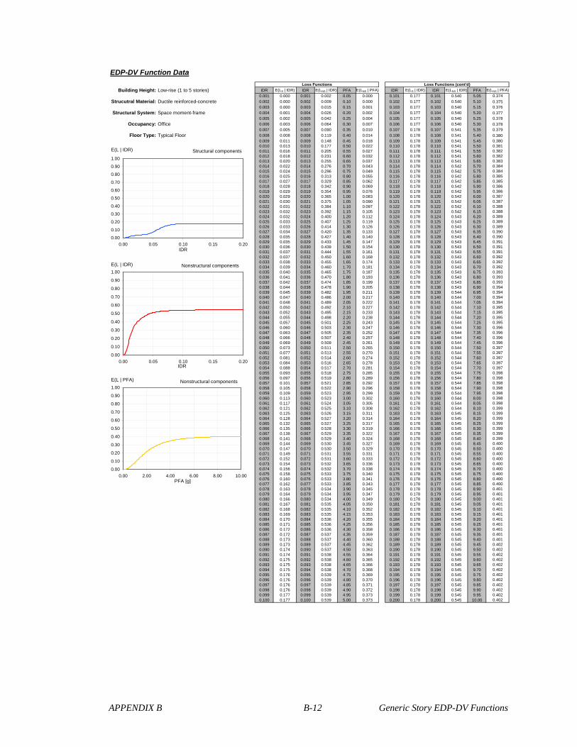
APPENDIX B B-12 Generic Story EDP-DV Functions
EDP-DV Function Data
Building Height: Low-rise (1 to 5 stories) IDR E(LS | IDR) IDR E(LNS | IDR) PFA E(LNS | PFA) IDR E(LS | IDR) IDR E(LNS | IDR) PFA E(LNS | PFA)
0.001 0.000 0.001 0.002 0.05 0.000 0.101 0.177 0.101 0.540 5.05 0.374
Strucutral Material: Ductile reinforced-concrete 0.002 0.000 0.002 0.009 0.10 0.000 0.102 0.177 0.102 0.540 5.10 0.3750.003 0.000 0.003 0.015 0.15 0.001 0.103 0.177 0.103 0.540 5.15 0.376
Structural System: Space moment-frame 0.004 0.001 0.004 0.026 0.20 0.002 0.104 0.177 0.104 0.540 5.20 0.3770.005 0.002 0.005 0.042 0.25 0.004 0.105 0.177 0.105 0.540 5.25 0.378
Occupancy: Office 0.006 0.003 0.006 0.064 0.30 0.007 0.106 0.177 0.106 0.540 5.30 0.3780.007 0.005 0.007 0.090 0.35 0.010 0.107 0.178 0.107 0.541 5.35 0.379
Floor Type: Typical Floor 0.008 0.008 0.008 0.119 0.40 0.014 0.108 0.178 0.108 0.541 5.40 0.3800.009 0.011 0.009 0.148 0.45 0.018 0.109 0.178 0.109 0.541 5.45 0.3800.010 0.013 0.010 0.177 0.50 0.022 0.110 0.178 0.110 0.541 5.50 0.3810.011 0.016 0.011 0.205 0.55 0.027 0.111 0.178 0.111 0.541 5.55 0.3820.012 0.018 0.012 0.231 0.60 0.032 0.112 0.178 0.112 0.541 5.60 0.3820.013 0.020 0.013 0.255 0.65 0.037 0.113 0.178 0.113 0.541 5.65 0.3830.014 0.022 0.014 0.276 0.70 0.043 0.114 0.178 0.114 0.542 5.70 0.3840.015 0.024 0.015 0.296 0.75 0.049 0.115 0.178 0.115 0.542 5.75 0.3840.016 0.025 0.016 0.313 0.80 0.055 0.116 0.178 0.116 0.542 5.80 0.3850.017 0.027 0.017 0.329 0.85 0.062 0.117 0.178 0.117 0.542 5.85 0.3850.018 0.028 0.018 0.342 0.90 0.069 0.118 0.178 0.118 0.542 5.90 0.3860.019 0.029 0.019 0.354 0.95 0.076 0.119 0.178 0.119 0.542 5.95 0.3860.020 0.029 0.020 0.365 1.00 0.083 0.120 0.178 0.120 0.542 6.00 0.3870.021 0.030 0.021 0.375 1.05 0.090 0.121 0.178 0.121 0.542 6.05 0.3870.022 0.031 0.022 0.384 1.10 0.097 0.122 0.178 0.122 0.542 6.10 0.3880.023 0.032 0.023 0.392 1.15 0.105 0.123 0.178 0.123 0.542 6.15 0.3880.024 0.032 0.024 0.400 1.20 0.112 0.124 0.178 0.124 0.543 6.20 0.3890.025 0.033 0.025 0.407 1.25 0.119 0.125 0.178 0.125 0.543 6.25 0.3890.026 0.033 0.026 0.414 1.30 0.126 0.126 0.178 0.126 0.543 6.30 0.3890.027 0.034 0.027 0.420 1.35 0.133 0.127 0.178 0.127 0.543 6.35 0.3900.028 0.035 0.028 0.427 1.40 0.140 0.128 0.178 0.128 0.543 6.40 0.3900.029 0.035 0.029 0.433 1.45 0.147 0.129 0.178 0.129 0.543 6.45 0.3910.030 0.036 0.030 0.439 1.50 0.154 0.130 0.178 0.130 0.543 6.50 0.3910.031 0.037 0.031 0.444 1.55 0.161 0.131 0.178 0.131 0.543 6.55 0.3910.032 0.037 0.032 0.450 1.60 0.168 0.132 0.178 0.132 0.543 6.60 0.3920.033 0.038 0.033 0.455 1.65 0.174 0.133 0.178 0.133 0.543 6.65 0.3920.034 0.039 0.034 0.460 1.70 0.181 0.134 0.178 0.134 0.543 6.70 0.3920.035 0.040 0.035 0.465 1.75 0.187 0.135 0.178 0.135 0.543 6.75 0.3930.036 0.041 0.036 0.470 1.80 0.193 0.136 0.178 0.136 0.543 6.80 0.3930.037 0.042 0.037 0.474 1.85 0.199 0.137 0.178 0.137 0.543 6.85 0.3930.038 0.044 0.038 0.478 1.90 0.205 0.138 0.178 0.138 0.543 6.90 0.3940.039 0.045 0.039 0.482 1.95 0.211 0.139 0.178 0.139 0.544 6.95 0.3940.040 0.047 0.040 0.486 2.00 0.217 0.140 0.178 0.140 0.544 7.00 0.3940.041 0.048 0.041 0.489 2.05 0.222 0.141 0.178 0.141 0.544 7.05 0.3940.042 0.050 0.042 0.492 2.10 0.227 0.142 0.178 0.142 0.544 7.10 0.3950.043 0.052 0.043 0.495 2.15 0.233 0.143 0.178 0.143 0.544 7.15 0.3950.044 0.055 0.044 0.498 2.20 0.238 0.144 0.178 0.144 0.544 7.20 0.3950.045 0.057 0.045 0.501 2.25 0.243 0.145 0.178 0.145 0.544 7.25 0.3950.046 0.060 0.046 0.503 2.30 0.247 0.146 0.178 0.146 0.544 7.30 0.3960.047 0.063 0.047 0.505 2.35 0.252 0.147 0.178 0.147 0.544 7.35 0.3960.048 0.066 0.048 0.507 2.40 0.257 0.148 0.178 0.148 0.544 7.40 0.3960.049 0.069 0.049 0.509 2.45 0.261 0.149 0.178 0.149 0.544 7.45 0.3960.050 0.073 0.050 0.511 2.50 0.265 0.150 0.178 0.150 0.544 7.50 0.3970.051 0.077 0.051 0.513 2.55 0.270 0.151 0.178 0.151 0.544 7.55 0.3970.052 0.081 0.052 0.514 2.60 0.274 0.152 0.178 0.152 0.544 7.60 0.3970.053 0.084 0.053 0.516 2.65 0.278 0.153 0.178 0.153 0.544 7.65 0.3970.054 0.088 0.054 0.517 2.70 0.281 0.154 0.178 0.154 0.544 7.70 0.3970.055 0.093 0.055 0.518 2.75 0.285 0.155 0.178 0.155 0.544 7.75 0.3980.056 0.097 0.056 0.519 2.80 0.289 0.156 0.178 0.156 0.544 7.80 0.3980.057 0.101 0.057 0.521 2.85 0.292 0.157 0.178 0.157 0.544 7.85 0.3980.058 0.105 0.058 0.522 2.90 0.296 0.158 0.178 0.158 0.544 7.90 0.3980.059 0.109 0.059 0.523 2.95 0.299 0.159 0.178 0.159 0.544 7.95 0.3980.060 0.113 0.060 0.523 3.00 0.302 0.160 0.178 0.160 0.544 8.00 0.3980.061 0.117 0.061 0.524 3.05 0.305 0.161 0.178 0.161 0.544 8.05 0.3980.062 0.121 0.062 0.525 3.10 0.308 0.162 0.178 0.162 0.544 8.10 0.3990.063 0.125 0.063 0.526 3.15 0.311 0.163 0.178 0.163 0.545 8.15 0.3990.064 0.128 0.064 0.527 3.20 0.314 0.164 0.178 0.164 0.545 8.20 0.3990.065 0.132 0.065 0.527 3.25 0.317 0.165 0.178 0.165 0.545 8.25 0.3990.066 0.135 0.066 0.528 3.30 0.319 0.166 0.178 0.166 0.545 8.30 0.3990.067 0.138 0.067 0.529 3.35 0.322 0.167 0.178 0.167 0.545 8.35 0.3990.068 0.141 0.068 0.529 3.40 0.324 0.168 0.178 0.168 0.545 8.40 0.3990.069 0.144 0.069 0.530 3.45 0.327 0.169 0.178 0.169 0.545 8.45 0.4000.070 0.147 0.070 0.530 3.50 0.329 0.170 0.178 0.170 0.545 8.50 0.4000.071 0.149 0.071 0.531 3.55 0.331 0.171 0.178 0.171 0.545 8.55 0.4000.072 0.152 0.072 0.531 3.60 0.333 0.172 0.178 0.172 0.545 8.60 0.4000.073 0.154 0.073 0.532 3.65 0.336 0.173 0.178 0.173 0.545 8.65 0.4000.074 0.156 0.074 0.532 3.70 0.338 0.174 0.178 0.174 0.545 8.70 0.4000.075 0.158 0.075 0.533 3.75 0.340 0.175 0.178 0.175 0.545 8.75 0.4000.076 0.160 0.076 0.533 3.80 0.341 0.176 0.178 0.176 0.545 8.80 0.4000.077 0.162 0.077 0.533 3.85 0.343 0.177 0.178 0.177 0.545 8.85 0.4000.078 0.163 0.078 0.534 3.90 0.345 0.178 0.178 0.178 0.545 8.90 0.4010.079 0.164 0.079 0.534 3.95 0.347 0.179 0.178 0.179 0.545 8.95 0.4010.080 0.166 0.080 0.534 4.00 0.349 0.180 0.178 0.180 0.545 9.00 0.4010.081 0.167 0.081 0.535 4.05 0.350 0.181 0.178 0.181 0.545 9.05 0.4010.082 0.168 0.082 0.535 4.10 0.352 0.182 0.178 0.182 0.545 9.10 0.4010.083 0.169 0.083 0.535 4.15 0.353 0.183 0.178 0.183 0.545 9.15 0.4010.084 0.170 0.084 0.536 4.20 0.355 0.184 0.178 0.184 0.545 9.20 0.4010.085 0.171 0.085 0.536 4.25 0.356 0.185 0.178 0.185 0.545 9.25 0.4010.086 0.172 0.086 0.536 4.30 0.358 0.186 0.178 0.186 0.545 9.30 0.4010.087 0.172 0.087 0.537 4.35 0.359 0.187 0.178 0.187 0.545 9.35 0.4010.088 0.173 0.088 0.537 4.40 0.360 0.188 0.178 0.188 0.545 9.40 0.4010.089 0.173 0.089 0.537 4.45 0.362 0.189 0.178 0.189 0.545 9.45 0.4020.090 0.174 0.090 0.537 4.50 0.363 0.190 0.178 0.190 0.545 9.50 0.4020.091 0.174 0.091 0.538 4.55 0.364 0.191 0.178 0.191 0.545 9.55 0.4020.092 0.175 0.092 0.538 4.60 0.365 0.192 0.178 0.192 0.545 9.60 0.4020.093 0.175 0.093 0.538 4.65 0.366 0.193 0.178 0.193 0.545 9.65 0.4020.094 0.175 0.094 0.538 4.70 0.368 0.194 0.178 0.194 0.545 9.70 0.4020.095 0.176 0.095 0.539 4.75 0.369 0.195 0.178 0.195 0.545 9.75 0.4020.096 0.176 0.096 0.539 4.80 0.370 0.196 0.178 0.196 0.545 9.80 0.4020.097 0.176 0.097 0.539 4.85 0.371 0.197 0.178 0.197 0.545 9.85 0.4020.098 0.176 0.098 0.539 4.90 0.372 0.198 0.178 0.198 0.545 9.90 0.4020.099 0.177 0.099 0.539 4.95 0.373 0.199 0.178 0.199 0.545 9.95 0.4020.100 0.177 0.100 0.539 5.00 0.373 0.200 0.178 0.200 0.545 10.00 0.402
Loss Functions Loss Functions (cont'd)
Structural components
0.00
0.10
0.20
0.30
0.40
0.50
0.60
0.70
0.80
0.90
1.00
0.00 0.05 0.10 0.15 0.20IDR
E(L | IDR)
Nonstructural components
0.00
0.10
0.20
0.30
0.40
0.50
0.60
0.70
0.80
0.90
1.00
0.00 0.05 0.10 0.15 0.20IDR
E(L | IDR)
Nonstructural components
0.00
0.10
0.20
0.30
0.40
0.50
0.60
0.70
0.80
0.90
1.00
0.00 2.00 4.00 6.00 8.00 10.00PFA [g]
E(L | PFA)

APPENDIX B B-13 Generic Story EDP-DV Functions
EDP-DV Function Data
Building Height: Low-rise (1 to 5 stories) IDR E(LS | IDR) IDR E(LNS | IDR) PFA E(LNS | PFA) IDR E(LS | IDR) IDR E(LNS | IDR) PFA E(LNS | PFA)
0.001 0.000 0.001 0.002 0.05 0.000 0.101 0.146 0.101 0.478 5.05 0.397
Strucutral Material: Ductile reinforced-concrete 0.002 0.000 0.002 0.007 0.10 0.000 0.102 0.146 0.102 0.479 5.10 0.3980.003 0.000 0.003 0.013 0.15 0.000 0.103 0.146 0.103 0.479 5.15 0.399
Structural System: Space moment-frame 0.004 0.000 0.004 0.021 0.20 0.001 0.104 0.146 0.104 0.479 5.20 0.4000.005 0.001 0.005 0.034 0.25 0.003 0.105 0.146 0.105 0.479 5.25 0.401
Occupancy: Office 0.006 0.003 0.006 0.052 0.30 0.005 0.106 0.146 0.106 0.479 5.30 0.4020.007 0.004 0.007 0.074 0.35 0.007 0.107 0.146 0.107 0.479 5.35 0.403
Floor Type: Top Floor 0.008 0.007 0.008 0.097 0.40 0.010 0.108 0.146 0.108 0.480 5.40 0.4040.009 0.009 0.009 0.122 0.45 0.013 0.109 0.146 0.109 0.480 5.45 0.4040.010 0.011 0.010 0.146 0.50 0.016 0.110 0.146 0.110 0.480 5.50 0.4050.011 0.013 0.011 0.169 0.55 0.020 0.111 0.146 0.111 0.480 5.55 0.4060.012 0.015 0.012 0.191 0.60 0.024 0.112 0.146 0.112 0.480 5.60 0.4070.013 0.017 0.013 0.211 0.65 0.029 0.113 0.146 0.113 0.480 5.65 0.4070.014 0.018 0.014 0.230 0.70 0.034 0.114 0.146 0.114 0.480 5.70 0.4080.015 0.020 0.015 0.246 0.75 0.040 0.115 0.146 0.115 0.480 5.75 0.4090.016 0.021 0.016 0.261 0.80 0.046 0.116 0.146 0.116 0.481 5.80 0.4100.017 0.022 0.017 0.275 0.85 0.052 0.117 0.146 0.117 0.481 5.85 0.4100.018 0.023 0.018 0.287 0.90 0.059 0.118 0.146 0.118 0.481 5.90 0.4110.019 0.024 0.019 0.297 0.95 0.065 0.119 0.146 0.119 0.481 5.95 0.4110.020 0.024 0.020 0.307 1.00 0.072 0.120 0.146 0.120 0.481 6.00 0.4120.021 0.025 0.021 0.315 1.05 0.079 0.121 0.146 0.121 0.481 6.05 0.4130.022 0.025 0.022 0.324 1.10 0.086 0.122 0.146 0.122 0.481 6.10 0.4130.023 0.026 0.023 0.331 1.15 0.094 0.123 0.146 0.123 0.481 6.15 0.4140.024 0.026 0.024 0.338 1.20 0.101 0.124 0.146 0.124 0.481 6.20 0.4140.025 0.027 0.025 0.345 1.25 0.109 0.125 0.146 0.125 0.481 6.25 0.4150.026 0.027 0.026 0.351 1.30 0.116 0.126 0.146 0.126 0.482 6.30 0.4150.027 0.028 0.027 0.358 1.35 0.123 0.127 0.146 0.127 0.482 6.35 0.4160.028 0.028 0.028 0.364 1.40 0.131 0.128 0.146 0.128 0.482 6.40 0.4160.029 0.029 0.029 0.370 1.45 0.138 0.129 0.146 0.129 0.482 6.45 0.4170.030 0.030 0.030 0.376 1.50 0.146 0.130 0.146 0.130 0.482 6.50 0.4170.031 0.030 0.031 0.381 1.55 0.153 0.131 0.146 0.131 0.482 6.55 0.4180.032 0.031 0.032 0.387 1.60 0.160 0.132 0.146 0.132 0.482 6.60 0.4180.033 0.031 0.033 0.392 1.65 0.167 0.133 0.146 0.133 0.482 6.65 0.4180.034 0.032 0.034 0.397 1.70 0.174 0.134 0.146 0.134 0.482 6.70 0.4190.035 0.033 0.035 0.402 1.75 0.181 0.135 0.146 0.135 0.482 6.75 0.4190.036 0.034 0.036 0.406 1.80 0.188 0.136 0.146 0.136 0.482 6.80 0.4200.037 0.035 0.037 0.411 1.85 0.194 0.137 0.146 0.137 0.482 6.85 0.4200.038 0.036 0.038 0.415 1.90 0.201 0.138 0.146 0.138 0.482 6.90 0.4200.039 0.037 0.039 0.419 1.95 0.207 0.139 0.146 0.139 0.482 6.95 0.4210.040 0.038 0.040 0.423 2.00 0.214 0.140 0.146 0.140 0.483 7.00 0.4210.041 0.040 0.041 0.426 2.05 0.220 0.141 0.146 0.141 0.483 7.05 0.4210.042 0.041 0.042 0.429 2.10 0.226 0.142 0.146 0.142 0.483 7.10 0.4220.043 0.043 0.043 0.432 2.15 0.232 0.143 0.146 0.143 0.483 7.15 0.4220.044 0.045 0.044 0.435 2.20 0.237 0.144 0.146 0.144 0.483 7.20 0.4220.045 0.047 0.045 0.438 2.25 0.243 0.145 0.146 0.145 0.483 7.25 0.4220.046 0.049 0.046 0.440 2.30 0.248 0.146 0.146 0.146 0.483 7.30 0.4230.047 0.052 0.047 0.443 2.35 0.254 0.147 0.146 0.147 0.483 7.35 0.4230.048 0.054 0.048 0.445 2.40 0.259 0.148 0.146 0.148 0.483 7.40 0.4230.049 0.057 0.049 0.447 2.45 0.264 0.149 0.146 0.149 0.483 7.45 0.4240.050 0.060 0.050 0.449 2.50 0.269 0.150 0.146 0.150 0.483 7.50 0.4240.051 0.063 0.051 0.450 2.55 0.274 0.151 0.146 0.151 0.483 7.55 0.4240.052 0.066 0.052 0.452 2.60 0.278 0.152 0.146 0.152 0.483 7.60 0.4240.053 0.069 0.053 0.454 2.65 0.283 0.153 0.146 0.153 0.483 7.65 0.4250.054 0.073 0.054 0.455 2.70 0.287 0.154 0.146 0.154 0.483 7.70 0.4250.055 0.076 0.055 0.456 2.75 0.292 0.155 0.146 0.155 0.483 7.75 0.4250.056 0.080 0.056 0.457 2.80 0.296 0.156 0.146 0.156 0.483 7.80 0.4250.057 0.083 0.057 0.459 2.85 0.300 0.157 0.146 0.157 0.483 7.85 0.4250.058 0.086 0.058 0.460 2.90 0.304 0.158 0.146 0.158 0.483 7.90 0.4260.059 0.090 0.059 0.461 2.95 0.308 0.159 0.146 0.159 0.483 7.95 0.4260.060 0.093 0.060 0.462 3.00 0.311 0.160 0.146 0.160 0.483 8.00 0.4260.061 0.096 0.061 0.462 3.05 0.315 0.161 0.146 0.161 0.483 8.05 0.4260.062 0.099 0.062 0.463 3.10 0.318 0.162 0.146 0.162 0.483 8.10 0.4260.063 0.102 0.063 0.464 3.15 0.322 0.163 0.146 0.163 0.483 8.15 0.4270.064 0.105 0.064 0.465 3.20 0.325 0.164 0.146 0.164 0.484 8.20 0.4270.065 0.108 0.065 0.466 3.25 0.328 0.165 0.146 0.165 0.484 8.25 0.4270.066 0.111 0.066 0.466 3.30 0.331 0.166 0.146 0.166 0.484 8.30 0.4270.067 0.114 0.067 0.467 3.35 0.334 0.167 0.146 0.167 0.484 8.35 0.4270.068 0.116 0.068 0.467 3.40 0.337 0.168 0.146 0.168 0.484 8.40 0.4270.069 0.119 0.069 0.468 3.45 0.340 0.169 0.146 0.169 0.484 8.45 0.4280.070 0.121 0.070 0.469 3.50 0.343 0.170 0.146 0.170 0.484 8.50 0.4280.071 0.123 0.071 0.469 3.55 0.346 0.171 0.146 0.171 0.484 8.55 0.4280.072 0.125 0.072 0.470 3.60 0.348 0.172 0.146 0.172 0.484 8.60 0.4280.073 0.127 0.073 0.470 3.65 0.351 0.173 0.146 0.173 0.484 8.65 0.4280.074 0.128 0.074 0.471 3.70 0.353 0.174 0.146 0.174 0.484 8.70 0.4280.075 0.130 0.075 0.471 3.75 0.356 0.175 0.146 0.175 0.484 8.75 0.4280.076 0.131 0.076 0.471 3.80 0.358 0.176 0.146 0.176 0.484 8.80 0.4280.077 0.133 0.077 0.472 3.85 0.360 0.177 0.146 0.177 0.484 8.85 0.4290.078 0.134 0.078 0.472 3.90 0.362 0.178 0.146 0.178 0.484 8.90 0.4290.079 0.135 0.079 0.473 3.95 0.364 0.179 0.146 0.179 0.484 8.95 0.4290.080 0.136 0.080 0.473 4.00 0.366 0.180 0.146 0.180 0.484 9.00 0.4290.081 0.137 0.081 0.473 4.05 0.368 0.181 0.146 0.181 0.484 9.05 0.4290.082 0.138 0.082 0.474 4.10 0.370 0.182 0.146 0.182 0.484 9.10 0.4290.083 0.139 0.083 0.474 4.15 0.372 0.183 0.146 0.183 0.484 9.15 0.4290.084 0.140 0.084 0.474 4.20 0.374 0.184 0.146 0.184 0.484 9.20 0.4290.085 0.140 0.085 0.475 4.25 0.376 0.185 0.146 0.185 0.484 9.25 0.4290.086 0.141 0.086 0.475 4.30 0.377 0.186 0.146 0.186 0.484 9.30 0.4300.087 0.142 0.087 0.475 4.35 0.379 0.187 0.146 0.187 0.484 9.35 0.4300.088 0.142 0.088 0.476 4.40 0.380 0.188 0.146 0.188 0.484 9.40 0.4300.089 0.143 0.089 0.476 4.45 0.382 0.189 0.146 0.189 0.484 9.45 0.4300.090 0.143 0.090 0.476 4.50 0.383 0.190 0.146 0.190 0.484 9.50 0.4300.091 0.143 0.091 0.476 4.55 0.385 0.191 0.146 0.191 0.484 9.55 0.4300.092 0.144 0.092 0.477 4.60 0.386 0.192 0.146 0.192 0.484 9.60 0.4300.093 0.144 0.093 0.477 4.65 0.388 0.193 0.146 0.193 0.484 9.65 0.4300.094 0.144 0.094 0.477 4.70 0.389 0.194 0.146 0.194 0.484 9.70 0.4300.095 0.145 0.095 0.477 4.75 0.390 0.195 0.146 0.195 0.484 9.75 0.4300.096 0.145 0.096 0.477 4.80 0.391 0.196 0.146 0.196 0.484 9.80 0.4300.097 0.145 0.097 0.478 4.85 0.393 0.197 0.146 0.197 0.484 9.85 0.4310.098 0.145 0.098 0.478 4.90 0.394 0.198 0.146 0.198 0.484 9.90 0.4310.099 0.145 0.099 0.478 4.95 0.395 0.199 0.146 0.199 0.484 9.95 0.4310.100 0.145 0.100 0.478 5.00 0.396 0.200 0.146 0.200 0.484 10.00 0.431
Loss Functions Loss Functions (cont'd)
Structural components
0.00
0.10
0.20
0.30
0.40
0.50
0.60
0.70
0.80
0.90
1.00
0.00 0.05 0.10 0.15 0.20IDR
E(L | IDR)
Nonstructural components
0.00
0.10
0.20
0.30
0.40
0.50
0.60
0.70
0.80
0.90
1.00
0.00 0.05 0.10 0.15 0.20IDR
E(L | IDR)
Nonstructural components
0.00
0.10
0.20
0.30
0.40
0.50
0.60
0.70
0.80
0.90
1.00
0.00 2.00 4.00 6.00 8.00 10.00PFA [g]
E(L | PFA)
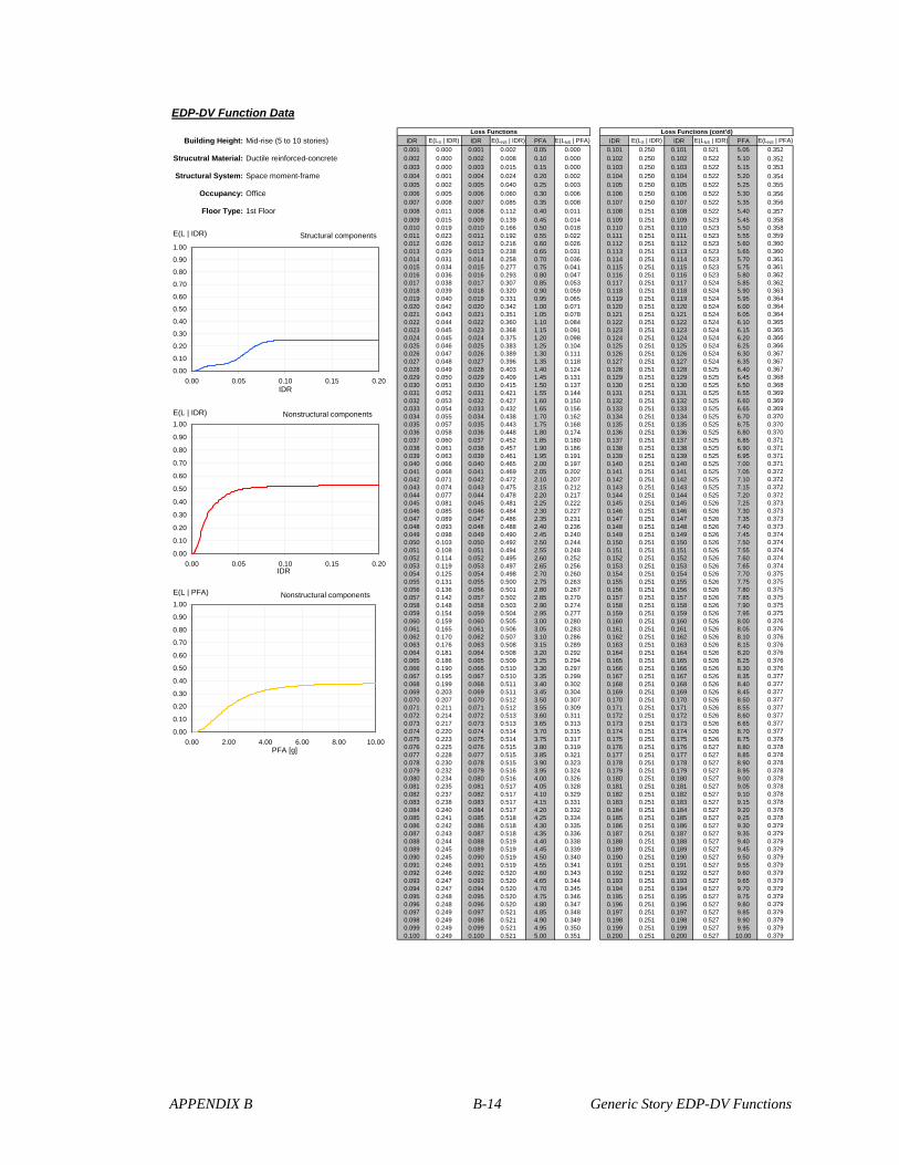
APPENDIX B B-14 Generic Story EDP-DV Functions
EDP-DV Function Data
Building Height: Mid-rise (5 to 10 stories) IDR E(LS | IDR) IDR E(LNS | IDR) PFA E(LNS | PFA) IDR E(LS | IDR) IDR E(LNS | IDR) PFA E(LNS | PFA)
0.001 0.000 0.001 0.002 0.05 0.000 0.101 0.250 0.101 0.521 5.05 0.352
Strucutral Material: Ductile reinforced-concrete 0.002 0.000 0.002 0.008 0.10 0.000 0.102 0.250 0.102 0.522 5.10 0.3520.003 0.000 0.003 0.015 0.15 0.000 0.103 0.250 0.103 0.522 5.15 0.353
Structural System: Space moment-frame 0.004 0.001 0.004 0.024 0.20 0.002 0.104 0.250 0.104 0.522 5.20 0.3540.005 0.002 0.005 0.040 0.25 0.003 0.105 0.250 0.105 0.522 5.25 0.355
Occupancy: Office 0.006 0.005 0.006 0.060 0.30 0.006 0.106 0.250 0.106 0.522 5.30 0.3560.007 0.008 0.007 0.085 0.35 0.008 0.107 0.250 0.107 0.522 5.35 0.356
Floor Type: 1st Floor 0.008 0.011 0.008 0.112 0.40 0.011 0.108 0.251 0.108 0.522 5.40 0.3570.009 0.015 0.009 0.139 0.45 0.014 0.109 0.251 0.109 0.523 5.45 0.3580.010 0.019 0.010 0.166 0.50 0.018 0.110 0.251 0.110 0.523 5.50 0.3580.011 0.023 0.011 0.192 0.55 0.022 0.111 0.251 0.111 0.523 5.55 0.3590.012 0.026 0.012 0.216 0.60 0.026 0.112 0.251 0.112 0.523 5.60 0.3600.013 0.029 0.013 0.238 0.65 0.031 0.113 0.251 0.113 0.523 5.65 0.3600.014 0.031 0.014 0.258 0.70 0.036 0.114 0.251 0.114 0.523 5.70 0.3610.015 0.034 0.015 0.277 0.75 0.041 0.115 0.251 0.115 0.523 5.75 0.3610.016 0.036 0.016 0.293 0.80 0.047 0.116 0.251 0.116 0.523 5.80 0.3620.017 0.038 0.017 0.307 0.85 0.053 0.117 0.251 0.117 0.524 5.85 0.3620.018 0.039 0.018 0.320 0.90 0.059 0.118 0.251 0.118 0.524 5.90 0.3630.019 0.040 0.019 0.331 0.95 0.065 0.119 0.251 0.119 0.524 5.95 0.3640.020 0.042 0.020 0.342 1.00 0.071 0.120 0.251 0.120 0.524 6.00 0.3640.021 0.043 0.021 0.351 1.05 0.078 0.121 0.251 0.121 0.524 6.05 0.3640.022 0.044 0.022 0.360 1.10 0.084 0.122 0.251 0.122 0.524 6.10 0.3650.023 0.045 0.023 0.368 1.15 0.091 0.123 0.251 0.123 0.524 6.15 0.3650.024 0.045 0.024 0.375 1.20 0.098 0.124 0.251 0.124 0.524 6.20 0.3660.025 0.046 0.025 0.383 1.25 0.104 0.125 0.251 0.125 0.524 6.25 0.3660.026 0.047 0.026 0.389 1.30 0.111 0.126 0.251 0.126 0.524 6.30 0.3670.027 0.048 0.027 0.396 1.35 0.118 0.127 0.251 0.127 0.524 6.35 0.3670.028 0.049 0.028 0.403 1.40 0.124 0.128 0.251 0.128 0.525 6.40 0.3670.029 0.050 0.029 0.409 1.45 0.131 0.129 0.251 0.129 0.525 6.45 0.3680.030 0.051 0.030 0.415 1.50 0.137 0.130 0.251 0.130 0.525 6.50 0.3680.031 0.052 0.031 0.421 1.55 0.144 0.131 0.251 0.131 0.525 6.55 0.3690.032 0.053 0.032 0.427 1.60 0.150 0.132 0.251 0.132 0.525 6.60 0.3690.033 0.054 0.033 0.432 1.65 0.156 0.133 0.251 0.133 0.525 6.65 0.3690.034 0.055 0.034 0.438 1.70 0.162 0.134 0.251 0.134 0.525 6.70 0.3700.035 0.057 0.035 0.443 1.75 0.168 0.135 0.251 0.135 0.525 6.75 0.3700.036 0.058 0.036 0.448 1.80 0.174 0.136 0.251 0.136 0.525 6.80 0.3700.037 0.060 0.037 0.452 1.85 0.180 0.137 0.251 0.137 0.525 6.85 0.3710.038 0.061 0.038 0.457 1.90 0.186 0.138 0.251 0.138 0.525 6.90 0.3710.039 0.063 0.039 0.461 1.95 0.191 0.139 0.251 0.139 0.525 6.95 0.3710.040 0.066 0.040 0.465 2.00 0.197 0.140 0.251 0.140 0.525 7.00 0.3710.041 0.068 0.041 0.469 2.05 0.202 0.141 0.251 0.141 0.525 7.05 0.3720.042 0.071 0.042 0.472 2.10 0.207 0.142 0.251 0.142 0.525 7.10 0.3720.043 0.074 0.043 0.475 2.15 0.212 0.143 0.251 0.143 0.525 7.15 0.3720.044 0.077 0.044 0.478 2.20 0.217 0.144 0.251 0.144 0.525 7.20 0.3720.045 0.081 0.045 0.481 2.25 0.222 0.145 0.251 0.145 0.526 7.25 0.3730.046 0.085 0.046 0.484 2.30 0.227 0.146 0.251 0.146 0.526 7.30 0.3730.047 0.089 0.047 0.486 2.35 0.231 0.147 0.251 0.147 0.526 7.35 0.3730.048 0.093 0.048 0.488 2.40 0.236 0.148 0.251 0.148 0.526 7.40 0.3730.049 0.098 0.049 0.490 2.45 0.240 0.149 0.251 0.149 0.526 7.45 0.3740.050 0.103 0.050 0.492 2.50 0.244 0.150 0.251 0.150 0.526 7.50 0.3740.051 0.108 0.051 0.494 2.55 0.248 0.151 0.251 0.151 0.526 7.55 0.3740.052 0.114 0.052 0.495 2.60 0.252 0.152 0.251 0.152 0.526 7.60 0.3740.053 0.119 0.053 0.497 2.65 0.256 0.153 0.251 0.153 0.526 7.65 0.3740.054 0.125 0.054 0.498 2.70 0.260 0.154 0.251 0.154 0.526 7.70 0.3750.055 0.131 0.055 0.500 2.75 0.263 0.155 0.251 0.155 0.526 7.75 0.3750.056 0.136 0.056 0.501 2.80 0.267 0.156 0.251 0.156 0.526 7.80 0.3750.057 0.142 0.057 0.502 2.85 0.270 0.157 0.251 0.157 0.526 7.85 0.3750.058 0.148 0.058 0.503 2.90 0.274 0.158 0.251 0.158 0.526 7.90 0.3750.059 0.154 0.059 0.504 2.95 0.277 0.159 0.251 0.159 0.526 7.95 0.3750.060 0.159 0.060 0.505 3.00 0.280 0.160 0.251 0.160 0.526 8.00 0.3760.061 0.165 0.061 0.506 3.05 0.283 0.161 0.251 0.161 0.526 8.05 0.3760.062 0.170 0.062 0.507 3.10 0.286 0.162 0.251 0.162 0.526 8.10 0.3760.063 0.176 0.063 0.508 3.15 0.289 0.163 0.251 0.163 0.526 8.15 0.3760.064 0.181 0.064 0.508 3.20 0.292 0.164 0.251 0.164 0.526 8.20 0.3760.065 0.186 0.065 0.509 3.25 0.294 0.165 0.251 0.165 0.526 8.25 0.3760.066 0.190 0.066 0.510 3.30 0.297 0.166 0.251 0.166 0.526 8.30 0.3760.067 0.195 0.067 0.510 3.35 0.299 0.167 0.251 0.167 0.526 8.35 0.3770.068 0.199 0.068 0.511 3.40 0.302 0.168 0.251 0.168 0.526 8.40 0.3770.069 0.203 0.069 0.511 3.45 0.304 0.169 0.251 0.169 0.526 8.45 0.3770.070 0.207 0.070 0.512 3.50 0.307 0.170 0.251 0.170 0.526 8.50 0.3770.071 0.211 0.071 0.512 3.55 0.309 0.171 0.251 0.171 0.526 8.55 0.3770.072 0.214 0.072 0.513 3.60 0.311 0.172 0.251 0.172 0.526 8.60 0.3770.073 0.217 0.073 0.513 3.65 0.313 0.173 0.251 0.173 0.526 8.65 0.3770.074 0.220 0.074 0.514 3.70 0.315 0.174 0.251 0.174 0.526 8.70 0.3770.075 0.223 0.075 0.514 3.75 0.317 0.175 0.251 0.175 0.526 8.75 0.3780.076 0.225 0.076 0.515 3.80 0.319 0.176 0.251 0.176 0.527 8.80 0.3780.077 0.228 0.077 0.515 3.85 0.321 0.177 0.251 0.177 0.527 8.85 0.3780.078 0.230 0.078 0.515 3.90 0.323 0.178 0.251 0.178 0.527 8.90 0.3780.079 0.232 0.079 0.516 3.95 0.324 0.179 0.251 0.179 0.527 8.95 0.3780.080 0.234 0.080 0.516 4.00 0.326 0.180 0.251 0.180 0.527 9.00 0.3780.081 0.235 0.081 0.517 4.05 0.328 0.181 0.251 0.181 0.527 9.05 0.3780.082 0.237 0.082 0.517 4.10 0.329 0.182 0.251 0.182 0.527 9.10 0.3780.083 0.238 0.083 0.517 4.15 0.331 0.183 0.251 0.183 0.527 9.15 0.3780.084 0.240 0.084 0.517 4.20 0.332 0.184 0.251 0.184 0.527 9.20 0.3780.085 0.241 0.085 0.518 4.25 0.334 0.185 0.251 0.185 0.527 9.25 0.3780.086 0.242 0.086 0.518 4.30 0.335 0.186 0.251 0.186 0.527 9.30 0.3790.087 0.243 0.087 0.518 4.35 0.336 0.187 0.251 0.187 0.527 9.35 0.3790.088 0.244 0.088 0.519 4.40 0.338 0.188 0.251 0.188 0.527 9.40 0.3790.089 0.245 0.089 0.519 4.45 0.339 0.189 0.251 0.189 0.527 9.45 0.3790.090 0.245 0.090 0.519 4.50 0.340 0.190 0.251 0.190 0.527 9.50 0.3790.091 0.246 0.091 0.519 4.55 0.341 0.191 0.251 0.191 0.527 9.55 0.3790.092 0.246 0.092 0.520 4.60 0.343 0.192 0.251 0.192 0.527 9.60 0.3790.093 0.247 0.093 0.520 4.65 0.344 0.193 0.251 0.193 0.527 9.65 0.3790.094 0.247 0.094 0.520 4.70 0.345 0.194 0.251 0.194 0.527 9.70 0.3790.095 0.248 0.095 0.520 4.75 0.346 0.195 0.251 0.195 0.527 9.75 0.3790.096 0.248 0.096 0.520 4.80 0.347 0.196 0.251 0.196 0.527 9.80 0.3790.097 0.249 0.097 0.521 4.85 0.348 0.197 0.251 0.197 0.527 9.85 0.3790.098 0.249 0.098 0.521 4.90 0.349 0.198 0.251 0.198 0.527 9.90 0.3790.099 0.249 0.099 0.521 4.95 0.350 0.199 0.251 0.199 0.527 9.95 0.3790.100 0.249 0.100 0.521 5.00 0.351 0.200 0.251 0.200 0.527 10.00 0.379
Loss Functions Loss Functions (cont'd)
Structural components
0.00
0.10
0.20
0.30
0.40
0.50
0.60
0.70
0.80
0.90
1.00
0.00 0.05 0.10 0.15 0.20IDR
E(L | IDR)
Nonstructural components
0.00
0.10
0.20
0.30
0.40
0.50
0.60
0.70
0.80
0.90
1.00
0.00 0.05 0.10 0.15 0.20IDR
E(L | IDR)
Nonstructural components
0.00
0.10
0.20
0.30
0.40
0.50
0.60
0.70
0.80
0.90
1.00
0.00 2.00 4.00 6.00 8.00 10.00PFA [g]
E(L | PFA)
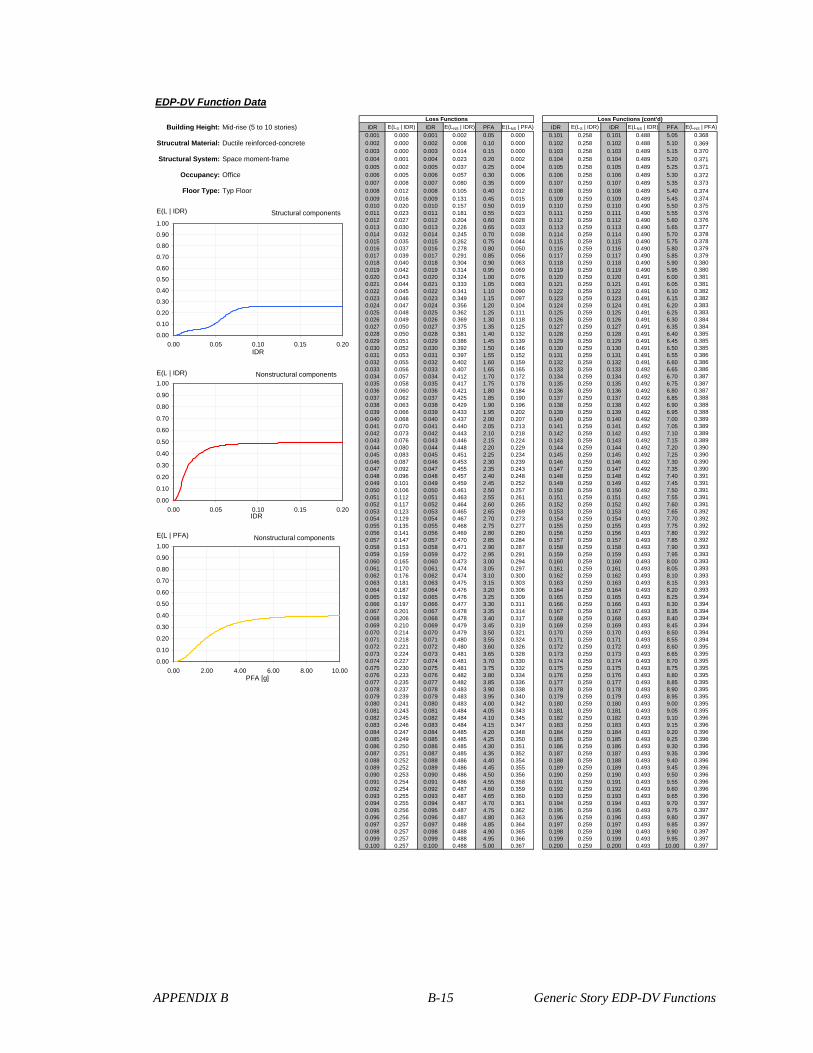
APPENDIX B B-15 Generic Story EDP-DV Functions
EDP-DV Function Data
Building Height: Mid-rise (5 to 10 stories) IDR E(LS | IDR) IDR E(LNS | IDR) PFA E(LNS | PFA) IDR E(LS | IDR) IDR E(LNS | IDR) PFA E(LNS | PFA)
0.001 0.000 0.001 0.002 0.05 0.000 0.101 0.258 0.101 0.488 5.05 0.368
Strucutral Material: Ductile reinforced-concrete 0.002 0.000 0.002 0.008 0.10 0.000 0.102 0.258 0.102 0.488 5.10 0.3690.003 0.000 0.003 0.014 0.15 0.000 0.103 0.258 0.103 0.489 5.15 0.370
Structural System: Space moment-frame 0.004 0.001 0.004 0.023 0.20 0.002 0.104 0.258 0.104 0.489 5.20 0.3710.005 0.002 0.005 0.037 0.25 0.004 0.105 0.258 0.105 0.489 5.25 0.371
Occupancy: Office 0.006 0.005 0.006 0.057 0.30 0.006 0.106 0.258 0.106 0.489 5.30 0.3720.007 0.008 0.007 0.080 0.35 0.009 0.107 0.259 0.107 0.489 5.35 0.373
Floor Type: Typ Floor 0.008 0.012 0.008 0.105 0.40 0.012 0.108 0.259 0.108 0.489 5.40 0.3740.009 0.016 0.009 0.131 0.45 0.015 0.109 0.259 0.109 0.489 5.45 0.3740.010 0.020 0.010 0.157 0.50 0.019 0.110 0.259 0.110 0.490 5.50 0.3750.011 0.023 0.011 0.181 0.55 0.023 0.111 0.259 0.111 0.490 5.55 0.3760.012 0.027 0.012 0.204 0.60 0.028 0.112 0.259 0.112 0.490 5.60 0.3760.013 0.030 0.013 0.226 0.65 0.033 0.113 0.259 0.113 0.490 5.65 0.3770.014 0.032 0.014 0.245 0.70 0.038 0.114 0.259 0.114 0.490 5.70 0.3780.015 0.035 0.015 0.262 0.75 0.044 0.115 0.259 0.115 0.490 5.75 0.3780.016 0.037 0.016 0.278 0.80 0.050 0.116 0.259 0.116 0.490 5.80 0.3790.017 0.039 0.017 0.291 0.85 0.056 0.117 0.259 0.117 0.490 5.85 0.3790.018 0.040 0.018 0.304 0.90 0.063 0.118 0.259 0.118 0.490 5.90 0.3800.019 0.042 0.019 0.314 0.95 0.069 0.119 0.259 0.119 0.490 5.95 0.3800.020 0.043 0.020 0.324 1.00 0.076 0.120 0.259 0.120 0.491 6.00 0.3810.021 0.044 0.021 0.333 1.05 0.083 0.121 0.259 0.121 0.491 6.05 0.3810.022 0.045 0.022 0.341 1.10 0.090 0.122 0.259 0.122 0.491 6.10 0.3820.023 0.046 0.023 0.349 1.15 0.097 0.123 0.259 0.123 0.491 6.15 0.3820.024 0.047 0.024 0.356 1.20 0.104 0.124 0.259 0.124 0.491 6.20 0.3830.025 0.048 0.025 0.362 1.25 0.111 0.125 0.259 0.125 0.491 6.25 0.3830.026 0.049 0.026 0.369 1.30 0.118 0.126 0.259 0.126 0.491 6.30 0.3840.027 0.050 0.027 0.375 1.35 0.125 0.127 0.259 0.127 0.491 6.35 0.3840.028 0.050 0.028 0.381 1.40 0.132 0.128 0.259 0.128 0.491 6.40 0.3850.029 0.051 0.029 0.386 1.45 0.139 0.129 0.259 0.129 0.491 6.45 0.3850.030 0.052 0.030 0.392 1.50 0.146 0.130 0.259 0.130 0.491 6.50 0.3850.031 0.053 0.031 0.397 1.55 0.152 0.131 0.259 0.131 0.491 6.55 0.3860.032 0.055 0.032 0.402 1.60 0.159 0.132 0.259 0.132 0.491 6.60 0.3860.033 0.056 0.033 0.407 1.65 0.165 0.133 0.259 0.133 0.492 6.65 0.3860.034 0.057 0.034 0.412 1.70 0.172 0.134 0.259 0.134 0.492 6.70 0.3870.035 0.058 0.035 0.417 1.75 0.178 0.135 0.259 0.135 0.492 6.75 0.3870.036 0.060 0.036 0.421 1.80 0.184 0.136 0.259 0.136 0.492 6.80 0.3870.037 0.062 0.037 0.425 1.85 0.190 0.137 0.259 0.137 0.492 6.85 0.3880.038 0.063 0.038 0.429 1.90 0.196 0.138 0.259 0.138 0.492 6.90 0.3880.039 0.066 0.039 0.433 1.95 0.202 0.139 0.259 0.139 0.492 6.95 0.3880.040 0.068 0.040 0.437 2.00 0.207 0.140 0.259 0.140 0.492 7.00 0.3890.041 0.070 0.041 0.440 2.05 0.213 0.141 0.259 0.141 0.492 7.05 0.3890.042 0.073 0.042 0.443 2.10 0.218 0.142 0.259 0.142 0.492 7.10 0.3890.043 0.076 0.043 0.446 2.15 0.224 0.143 0.259 0.143 0.492 7.15 0.3890.044 0.080 0.044 0.448 2.20 0.229 0.144 0.259 0.144 0.492 7.20 0.3900.045 0.083 0.045 0.451 2.25 0.234 0.145 0.259 0.145 0.492 7.25 0.3900.046 0.087 0.046 0.453 2.30 0.239 0.146 0.259 0.146 0.492 7.30 0.3900.047 0.092 0.047 0.455 2.35 0.243 0.147 0.259 0.147 0.492 7.35 0.3900.048 0.096 0.048 0.457 2.40 0.248 0.148 0.259 0.148 0.492 7.40 0.3910.049 0.101 0.049 0.459 2.45 0.252 0.149 0.259 0.149 0.492 7.45 0.3910.050 0.106 0.050 0.461 2.50 0.257 0.150 0.259 0.150 0.492 7.50 0.3910.051 0.112 0.051 0.463 2.55 0.261 0.151 0.259 0.151 0.492 7.55 0.3910.052 0.117 0.052 0.464 2.60 0.265 0.152 0.259 0.152 0.492 7.60 0.3910.053 0.123 0.053 0.465 2.65 0.269 0.153 0.259 0.153 0.492 7.65 0.3920.054 0.129 0.054 0.467 2.70 0.273 0.154 0.259 0.154 0.493 7.70 0.3920.055 0.135 0.055 0.468 2.75 0.277 0.155 0.259 0.155 0.493 7.75 0.3920.056 0.141 0.056 0.469 2.80 0.280 0.156 0.259 0.156 0.493 7.80 0.3920.057 0.147 0.057 0.470 2.85 0.284 0.157 0.259 0.157 0.493 7.85 0.3920.058 0.153 0.058 0.471 2.90 0.287 0.158 0.259 0.158 0.493 7.90 0.3930.059 0.159 0.059 0.472 2.95 0.291 0.159 0.259 0.159 0.493 7.95 0.3930.060 0.165 0.060 0.473 3.00 0.294 0.160 0.259 0.160 0.493 8.00 0.3930.061 0.170 0.061 0.474 3.05 0.297 0.161 0.259 0.161 0.493 8.05 0.3930.062 0.176 0.062 0.474 3.10 0.300 0.162 0.259 0.162 0.493 8.10 0.3930.063 0.181 0.063 0.475 3.15 0.303 0.163 0.259 0.163 0.493 8.15 0.3930.064 0.187 0.064 0.476 3.20 0.306 0.164 0.259 0.164 0.493 8.20 0.3930.065 0.192 0.065 0.476 3.25 0.309 0.165 0.259 0.165 0.493 8.25 0.3940.066 0.197 0.066 0.477 3.30 0.311 0.166 0.259 0.166 0.493 8.30 0.3940.067 0.201 0.067 0.478 3.35 0.314 0.167 0.259 0.167 0.493 8.35 0.3940.068 0.206 0.068 0.478 3.40 0.317 0.168 0.259 0.168 0.493 8.40 0.3940.069 0.210 0.069 0.479 3.45 0.319 0.169 0.259 0.169 0.493 8.45 0.3940.070 0.214 0.070 0.479 3.50 0.321 0.170 0.259 0.170 0.493 8.50 0.3940.071 0.218 0.071 0.480 3.55 0.324 0.171 0.259 0.171 0.493 8.55 0.3940.072 0.221 0.072 0.480 3.60 0.326 0.172 0.259 0.172 0.493 8.60 0.3950.073 0.224 0.073 0.481 3.65 0.328 0.173 0.259 0.173 0.493 8.65 0.3950.074 0.227 0.074 0.481 3.70 0.330 0.174 0.259 0.174 0.493 8.70 0.3950.075 0.230 0.075 0.481 3.75 0.332 0.175 0.259 0.175 0.493 8.75 0.3950.076 0.233 0.076 0.482 3.80 0.334 0.176 0.259 0.176 0.493 8.80 0.3950.077 0.235 0.077 0.482 3.85 0.336 0.177 0.259 0.177 0.493 8.85 0.3950.078 0.237 0.078 0.483 3.90 0.338 0.178 0.259 0.178 0.493 8.90 0.3950.079 0.239 0.079 0.483 3.95 0.340 0.179 0.259 0.179 0.493 8.95 0.3950.080 0.241 0.080 0.483 4.00 0.342 0.180 0.259 0.180 0.493 9.00 0.3950.081 0.243 0.081 0.484 4.05 0.343 0.181 0.259 0.181 0.493 9.05 0.3950.082 0.245 0.082 0.484 4.10 0.345 0.182 0.259 0.182 0.493 9.10 0.3960.083 0.246 0.083 0.484 4.15 0.347 0.183 0.259 0.183 0.493 9.15 0.3960.084 0.247 0.084 0.485 4.20 0.348 0.184 0.259 0.184 0.493 9.20 0.3960.085 0.249 0.085 0.485 4.25 0.350 0.185 0.259 0.185 0.493 9.25 0.3960.086 0.250 0.086 0.485 4.30 0.351 0.186 0.259 0.186 0.493 9.30 0.3960.087 0.251 0.087 0.485 4.35 0.352 0.187 0.259 0.187 0.493 9.35 0.3960.088 0.252 0.088 0.486 4.40 0.354 0.188 0.259 0.188 0.493 9.40 0.3960.089 0.252 0.089 0.486 4.45 0.355 0.189 0.259 0.189 0.493 9.45 0.3960.090 0.253 0.090 0.486 4.50 0.356 0.190 0.259 0.190 0.493 9.50 0.3960.091 0.254 0.091 0.486 4.55 0.358 0.191 0.259 0.191 0.493 9.55 0.3960.092 0.254 0.092 0.487 4.60 0.359 0.192 0.259 0.192 0.493 9.60 0.3960.093 0.255 0.093 0.487 4.65 0.360 0.193 0.259 0.193 0.493 9.65 0.3960.094 0.255 0.094 0.487 4.70 0.361 0.194 0.259 0.194 0.493 9.70 0.3970.095 0.256 0.095 0.487 4.75 0.362 0.195 0.259 0.195 0.493 9.75 0.3970.096 0.256 0.096 0.487 4.80 0.363 0.196 0.259 0.196 0.493 9.80 0.3970.097 0.257 0.097 0.488 4.85 0.364 0.197 0.259 0.197 0.493 9.85 0.3970.098 0.257 0.098 0.488 4.90 0.365 0.198 0.259 0.198 0.493 9.90 0.3970.099 0.257 0.099 0.488 4.95 0.366 0.199 0.259 0.199 0.493 9.95 0.3970.100 0.257 0.100 0.488 5.00 0.367 0.200 0.259 0.200 0.493 10.00 0.397
Loss Functions Loss Functions (cont'd)
Structural components
0.00
0.10
0.20
0.30
0.40
0.50
0.60
0.70
0.80
0.90
1.00
0.00 0.05 0.10 0.15 0.20IDR
E(L | IDR)
Nonstructural components
0.00
0.10
0.20
0.30
0.40
0.50
0.60
0.70
0.80
0.90
1.00
0.00 0.05 0.10 0.15 0.20IDR
E(L | IDR)
Nonstructural components
0.00
0.10
0.20
0.30
0.40
0.50
0.60
0.70
0.80
0.90
1.00
0.00 2.00 4.00 6.00 8.00 10.00PFA [g]
E(L | PFA)

APPENDIX B B-16 Generic Story EDP-DV Functions
EDP-DV Function Data
Building Height: Mid-rise (5 to 10 stories) IDR E(LS | IDR) IDR E(LNS | IDR) PFA E(LNS | PFA) IDR E(LS | IDR) IDR E(LNS | IDR) PFA E(LNS | PFA)
0.001 0.000 0.001 0.001 0.05 0.000 0.101 0.215 0.101 0.453 5.05 0.404
Strucutral Material: Ductile reinforced-concrete 0.002 0.000 0.002 0.006 0.10 0.000 0.102 0.215 0.102 0.453 5.10 0.4050.003 0.000 0.003 0.012 0.15 0.000 0.103 0.215 0.103 0.453 5.15 0.406
Structural System: Space moment-frame 0.004 0.001 0.004 0.020 0.20 0.001 0.104 0.215 0.104 0.453 5.20 0.4070.005 0.002 0.005 0.032 0.25 0.003 0.105 0.215 0.105 0.453 5.25 0.408
Occupancy: Office 0.006 0.004 0.006 0.049 0.30 0.004 0.106 0.215 0.106 0.454 5.30 0.4090.007 0.007 0.007 0.069 0.35 0.007 0.107 0.215 0.107 0.454 5.35 0.410
Floor Type: Top Floor 0.008 0.010 0.008 0.091 0.40 0.009 0.108 0.216 0.108 0.454 5.40 0.4110.009 0.013 0.009 0.114 0.45 0.012 0.109 0.216 0.109 0.454 5.45 0.4110.010 0.016 0.010 0.136 0.50 0.015 0.110 0.216 0.110 0.454 5.50 0.4120.011 0.019 0.011 0.158 0.55 0.019 0.111 0.216 0.111 0.454 5.55 0.4130.012 0.022 0.012 0.178 0.60 0.023 0.112 0.216 0.112 0.454 5.60 0.4140.013 0.025 0.013 0.197 0.65 0.028 0.113 0.216 0.113 0.454 5.65 0.4150.014 0.027 0.014 0.214 0.70 0.033 0.114 0.216 0.114 0.455 5.70 0.4150.015 0.029 0.015 0.230 0.75 0.038 0.115 0.216 0.115 0.455 5.75 0.4160.016 0.031 0.016 0.244 0.80 0.044 0.116 0.216 0.116 0.455 5.80 0.4170.017 0.032 0.017 0.256 0.85 0.050 0.117 0.216 0.117 0.455 5.85 0.4180.018 0.034 0.018 0.267 0.90 0.057 0.118 0.216 0.118 0.455 5.90 0.4180.019 0.035 0.019 0.277 0.95 0.064 0.119 0.216 0.119 0.455 5.95 0.4190.020 0.036 0.020 0.286 1.00 0.071 0.120 0.216 0.120 0.455 6.00 0.4190.021 0.037 0.021 0.294 1.05 0.078 0.121 0.216 0.121 0.455 6.05 0.4200.022 0.038 0.022 0.302 1.10 0.085 0.122 0.216 0.122 0.455 6.10 0.4210.023 0.038 0.023 0.309 1.15 0.092 0.123 0.216 0.123 0.456 6.15 0.4210.024 0.039 0.024 0.316 1.20 0.100 0.124 0.216 0.124 0.456 6.20 0.4220.025 0.040 0.025 0.322 1.25 0.107 0.125 0.216 0.125 0.456 6.25 0.4220.026 0.041 0.026 0.328 1.30 0.115 0.126 0.216 0.126 0.456 6.30 0.4230.027 0.041 0.027 0.335 1.35 0.122 0.127 0.216 0.127 0.456 6.35 0.4230.028 0.042 0.028 0.340 1.40 0.130 0.128 0.216 0.128 0.456 6.40 0.4240.029 0.043 0.029 0.346 1.45 0.137 0.129 0.216 0.129 0.456 6.45 0.4240.030 0.044 0.030 0.352 1.50 0.145 0.130 0.216 0.130 0.456 6.50 0.4250.031 0.045 0.031 0.357 1.55 0.152 0.131 0.216 0.131 0.456 6.55 0.4250.032 0.045 0.032 0.363 1.60 0.160 0.132 0.216 0.132 0.456 6.60 0.4260.033 0.046 0.033 0.368 1.65 0.167 0.133 0.216 0.133 0.456 6.65 0.4260.034 0.048 0.034 0.373 1.70 0.174 0.134 0.216 0.134 0.456 6.70 0.4260.035 0.049 0.035 0.377 1.75 0.181 0.135 0.216 0.135 0.456 6.75 0.4270.036 0.050 0.036 0.382 1.80 0.188 0.136 0.216 0.136 0.456 6.80 0.4270.037 0.051 0.037 0.386 1.85 0.195 0.137 0.216 0.137 0.457 6.85 0.4280.038 0.053 0.038 0.390 1.90 0.201 0.138 0.216 0.138 0.457 6.90 0.4280.039 0.055 0.039 0.394 1.95 0.208 0.139 0.216 0.139 0.457 6.95 0.4280.040 0.057 0.040 0.398 2.00 0.214 0.140 0.216 0.140 0.457 7.00 0.4290.041 0.059 0.041 0.401 2.05 0.221 0.141 0.216 0.141 0.457 7.05 0.4290.042 0.061 0.042 0.405 2.10 0.227 0.142 0.216 0.142 0.457 7.10 0.4290.043 0.064 0.043 0.408 2.15 0.233 0.143 0.216 0.143 0.457 7.15 0.4300.044 0.066 0.044 0.410 2.20 0.239 0.144 0.216 0.144 0.457 7.20 0.4300.045 0.069 0.045 0.413 2.25 0.244 0.145 0.216 0.145 0.457 7.25 0.4300.046 0.073 0.046 0.415 2.30 0.250 0.146 0.216 0.146 0.457 7.30 0.4310.047 0.076 0.047 0.418 2.35 0.256 0.147 0.216 0.147 0.457 7.35 0.4310.048 0.080 0.048 0.420 2.40 0.261 0.148 0.216 0.148 0.457 7.40 0.4310.049 0.084 0.049 0.422 2.45 0.266 0.149 0.216 0.149 0.457 7.45 0.4310.050 0.089 0.050 0.424 2.50 0.271 0.150 0.216 0.150 0.457 7.50 0.4320.051 0.093 0.051 0.425 2.55 0.276 0.151 0.216 0.151 0.457 7.55 0.4320.052 0.098 0.052 0.427 2.60 0.281 0.152 0.216 0.152 0.457 7.60 0.4320.053 0.102 0.053 0.428 2.65 0.286 0.153 0.216 0.153 0.457 7.65 0.4320.054 0.107 0.054 0.430 2.70 0.290 0.154 0.216 0.154 0.457 7.70 0.4330.055 0.112 0.055 0.431 2.75 0.295 0.155 0.216 0.155 0.457 7.75 0.4330.056 0.117 0.056 0.432 2.80 0.299 0.156 0.216 0.156 0.457 7.80 0.4330.057 0.122 0.057 0.433 2.85 0.303 0.157 0.216 0.157 0.457 7.85 0.4330.058 0.127 0.058 0.434 2.90 0.307 0.158 0.216 0.158 0.457 7.90 0.4340.059 0.132 0.059 0.435 2.95 0.311 0.159 0.216 0.159 0.458 7.95 0.4340.060 0.137 0.060 0.436 3.00 0.315 0.160 0.216 0.160 0.458 8.00 0.4340.061 0.142 0.061 0.437 3.05 0.319 0.161 0.216 0.161 0.458 8.05 0.4340.062 0.147 0.062 0.438 3.10 0.322 0.162 0.216 0.162 0.458 8.10 0.4340.063 0.151 0.063 0.439 3.15 0.326 0.163 0.216 0.163 0.458 8.15 0.4350.064 0.156 0.064 0.439 3.20 0.329 0.164 0.216 0.164 0.458 8.20 0.4350.065 0.160 0.065 0.440 3.25 0.333 0.165 0.216 0.165 0.458 8.25 0.4350.066 0.164 0.066 0.441 3.30 0.336 0.166 0.216 0.166 0.458 8.30 0.4350.067 0.168 0.067 0.441 3.35 0.339 0.167 0.216 0.167 0.458 8.35 0.4350.068 0.171 0.068 0.442 3.40 0.342 0.168 0.216 0.168 0.458 8.40 0.4350.069 0.175 0.069 0.443 3.45 0.345 0.169 0.216 0.169 0.458 8.45 0.4360.070 0.178 0.070 0.443 3.50 0.348 0.170 0.216 0.170 0.458 8.50 0.4360.071 0.181 0.071 0.444 3.55 0.351 0.171 0.216 0.171 0.458 8.55 0.4360.072 0.184 0.072 0.444 3.60 0.353 0.172 0.216 0.172 0.458 8.60 0.4360.073 0.187 0.073 0.445 3.65 0.356 0.173 0.216 0.173 0.458 8.65 0.4360.074 0.189 0.074 0.445 3.70 0.358 0.174 0.216 0.174 0.458 8.70 0.4360.075 0.192 0.075 0.445 3.75 0.361 0.175 0.216 0.175 0.458 8.75 0.4360.076 0.194 0.076 0.446 3.80 0.363 0.176 0.216 0.176 0.458 8.80 0.4370.077 0.196 0.077 0.446 3.85 0.365 0.177 0.216 0.177 0.458 8.85 0.4370.078 0.198 0.078 0.447 3.90 0.368 0.178 0.216 0.178 0.458 8.90 0.4370.079 0.200 0.079 0.447 3.95 0.370 0.179 0.216 0.179 0.458 8.95 0.4370.080 0.201 0.080 0.447 4.00 0.372 0.180 0.216 0.180 0.458 9.00 0.4370.081 0.203 0.081 0.448 4.05 0.374 0.181 0.216 0.181 0.458 9.05 0.4370.082 0.204 0.082 0.448 4.10 0.376 0.182 0.216 0.182 0.458 9.10 0.4370.083 0.205 0.083 0.448 4.15 0.378 0.183 0.216 0.183 0.458 9.15 0.4370.084 0.206 0.084 0.449 4.20 0.380 0.184 0.216 0.184 0.458 9.20 0.4370.085 0.207 0.085 0.449 4.25 0.382 0.185 0.216 0.185 0.458 9.25 0.4380.086 0.208 0.086 0.449 4.30 0.383 0.186 0.216 0.186 0.458 9.30 0.4380.087 0.209 0.087 0.450 4.35 0.385 0.187 0.216 0.187 0.458 9.35 0.4380.088 0.210 0.088 0.450 4.40 0.387 0.188 0.216 0.188 0.458 9.40 0.4380.089 0.210 0.089 0.450 4.45 0.388 0.189 0.216 0.189 0.458 9.45 0.4380.090 0.211 0.090 0.450 4.50 0.390 0.190 0.216 0.190 0.458 9.50 0.4380.091 0.212 0.091 0.451 4.55 0.391 0.191 0.216 0.191 0.458 9.55 0.4380.092 0.212 0.092 0.451 4.60 0.393 0.192 0.216 0.192 0.458 9.60 0.4380.093 0.213 0.093 0.451 4.65 0.394 0.193 0.216 0.193 0.458 9.65 0.4380.094 0.213 0.094 0.451 4.70 0.395 0.194 0.216 0.194 0.458 9.70 0.4380.095 0.213 0.095 0.452 4.75 0.397 0.195 0.216 0.195 0.458 9.75 0.4380.096 0.214 0.096 0.452 4.80 0.398 0.196 0.216 0.196 0.458 9.80 0.4390.097 0.214 0.097 0.452 4.85 0.399 0.197 0.216 0.197 0.458 9.85 0.4390.098 0.214 0.098 0.452 4.90 0.400 0.198 0.216 0.198 0.458 9.90 0.4390.099 0.214 0.099 0.452 4.95 0.402 0.199 0.216 0.199 0.458 9.95 0.4390.100 0.215 0.100 0.453 5.00 0.403 0.200 0.216 0.200 0.458 10.00 0.439
Loss Functions Loss Functions (cont'd)
Structural components
0.00
0.10
0.20
0.30
0.40
0.50
0.60
0.70
0.80
0.90
1.00
0.00 0.05 0.10 0.15 0.20IDR
E(L | IDR)
Nonstructural components
0.00
0.10
0.20
0.30
0.40
0.50
0.60
0.70
0.80
0.90
1.00
0.00 0.05 0.10 0.15 0.20IDR
E(L | IDR)
Nonstructural components
0.00
0.10
0.20
0.30
0.40
0.50
0.60
0.70
0.80
0.90
1.00
0.00 2.00 4.00 6.00 8.00 10.00PFA [g]
E(L | PFA)

APPENDIX B B-17 Generic Story EDP-DV Functions
EDP-DV Function Data
Building Height: High-rise (>10 stories) IDR E(LS | IDR) IDR E(LNS | IDR) PFA E(LNS | PFA) IDR E(LS | IDR) IDR E(LNS | IDR) PFA E(LNS | PFA)
0.001 0.000 0.001 0.002 0.05 0.000 0.101 0.321 0.101 0.479 5.05 0.342
Strucutral Material: Ductile reinforced-concrete 0.002 0.000 0.002 0.007 0.10 0.000 0.102 0.322 0.102 0.479 5.10 0.3430.003 0.000 0.003 0.013 0.15 0.000 0.103 0.322 0.103 0.479 5.15 0.344
Structural System: Space moment-frame 0.004 0.001 0.004 0.022 0.20 0.001 0.104 0.322 0.104 0.479 5.20 0.3450.005 0.003 0.005 0.035 0.25 0.003 0.105 0.322 0.105 0.479 5.25 0.345
Occupancy: Office 0.006 0.006 0.006 0.054 0.30 0.005 0.106 0.322 0.106 0.479 5.30 0.3460.007 0.010 0.007 0.076 0.35 0.007 0.107 0.322 0.107 0.479 5.35 0.347
Floor Type: 1st Floor 0.008 0.015 0.008 0.099 0.40 0.010 0.108 0.322 0.108 0.480 5.40 0.3480.009 0.019 0.009 0.124 0.45 0.013 0.109 0.323 0.109 0.480 5.45 0.3480.010 0.024 0.010 0.148 0.50 0.016 0.110 0.323 0.110 0.480 5.50 0.3490.011 0.029 0.011 0.172 0.55 0.020 0.111 0.323 0.111 0.480 5.55 0.3500.012 0.033 0.012 0.194 0.60 0.024 0.112 0.323 0.112 0.480 5.60 0.3500.013 0.037 0.013 0.214 0.65 0.028 0.113 0.323 0.113 0.480 5.65 0.3510.014 0.041 0.014 0.232 0.70 0.033 0.114 0.323 0.114 0.480 5.70 0.3510.015 0.043 0.015 0.249 0.75 0.038 0.115 0.323 0.115 0.481 5.75 0.3520.016 0.046 0.016 0.264 0.80 0.044 0.116 0.323 0.116 0.481 5.80 0.3530.017 0.048 0.017 0.277 0.85 0.049 0.117 0.323 0.117 0.481 5.85 0.3530.018 0.050 0.018 0.289 0.90 0.055 0.118 0.323 0.118 0.481 5.90 0.3540.019 0.052 0.019 0.299 0.95 0.061 0.119 0.323 0.119 0.481 5.95 0.3540.020 0.054 0.020 0.309 1.00 0.067 0.120 0.323 0.120 0.481 6.00 0.3550.021 0.055 0.021 0.317 1.05 0.074 0.121 0.323 0.121 0.481 6.05 0.3550.022 0.056 0.022 0.325 1.10 0.080 0.122 0.323 0.122 0.481 6.10 0.3560.023 0.057 0.023 0.333 1.15 0.086 0.123 0.323 0.123 0.481 6.15 0.3560.024 0.058 0.024 0.340 1.20 0.093 0.124 0.323 0.124 0.481 6.20 0.3560.025 0.060 0.025 0.347 1.25 0.099 0.125 0.323 0.125 0.482 6.25 0.3570.026 0.061 0.026 0.353 1.30 0.106 0.126 0.323 0.126 0.482 6.30 0.3570.027 0.062 0.027 0.359 1.35 0.112 0.127 0.323 0.127 0.482 6.35 0.3580.028 0.063 0.028 0.365 1.40 0.119 0.128 0.323 0.128 0.482 6.40 0.3580.029 0.064 0.029 0.371 1.45 0.125 0.129 0.323 0.129 0.482 6.45 0.3580.030 0.065 0.030 0.377 1.50 0.131 0.130 0.323 0.130 0.482 6.50 0.3590.031 0.067 0.031 0.382 1.55 0.137 0.131 0.323 0.131 0.482 6.55 0.3590.032 0.068 0.032 0.388 1.60 0.144 0.132 0.323 0.132 0.482 6.60 0.3600.033 0.070 0.033 0.393 1.65 0.150 0.133 0.323 0.133 0.482 6.65 0.3600.034 0.071 0.034 0.398 1.70 0.156 0.134 0.323 0.134 0.482 6.70 0.3600.035 0.073 0.035 0.403 1.75 0.162 0.135 0.323 0.135 0.482 6.75 0.3600.036 0.075 0.036 0.407 1.80 0.167 0.136 0.323 0.136 0.482 6.80 0.3610.037 0.077 0.037 0.411 1.85 0.173 0.137 0.323 0.137 0.482 6.85 0.3610.038 0.079 0.038 0.416 1.90 0.178 0.138 0.323 0.138 0.483 6.90 0.3610.039 0.082 0.039 0.419 1.95 0.184 0.139 0.323 0.139 0.483 6.95 0.3620.040 0.085 0.040 0.423 2.00 0.189 0.140 0.323 0.140 0.483 7.00 0.3620.041 0.088 0.041 0.427 2.05 0.194 0.141 0.323 0.141 0.483 7.05 0.3620.042 0.091 0.042 0.430 2.10 0.199 0.142 0.323 0.142 0.483 7.10 0.3620.043 0.095 0.043 0.433 2.15 0.204 0.143 0.323 0.143 0.483 7.15 0.3630.044 0.099 0.044 0.436 2.20 0.209 0.144 0.323 0.144 0.483 7.20 0.3630.045 0.104 0.045 0.438 2.25 0.214 0.145 0.323 0.145 0.483 7.25 0.3630.046 0.109 0.046 0.441 2.30 0.219 0.146 0.323 0.146 0.483 7.30 0.3630.047 0.114 0.047 0.443 2.35 0.223 0.147 0.323 0.147 0.483 7.35 0.3640.048 0.120 0.048 0.445 2.40 0.227 0.148 0.323 0.148 0.483 7.40 0.3640.049 0.126 0.049 0.447 2.45 0.232 0.149 0.323 0.149 0.483 7.45 0.3640.050 0.133 0.050 0.449 2.50 0.236 0.150 0.323 0.150 0.483 7.50 0.3640.051 0.139 0.051 0.451 2.55 0.240 0.151 0.323 0.151 0.483 7.55 0.3650.052 0.146 0.052 0.452 2.60 0.244 0.152 0.323 0.152 0.483 7.60 0.3650.053 0.153 0.053 0.454 2.65 0.248 0.153 0.323 0.153 0.483 7.65 0.3650.054 0.161 0.054 0.455 2.70 0.251 0.154 0.323 0.154 0.483 7.70 0.3650.055 0.168 0.055 0.456 2.75 0.255 0.155 0.323 0.155 0.483 7.75 0.3650.056 0.176 0.056 0.458 2.80 0.258 0.156 0.323 0.156 0.483 7.80 0.3650.057 0.183 0.057 0.459 2.85 0.262 0.157 0.323 0.157 0.483 7.85 0.3660.058 0.191 0.058 0.460 2.90 0.265 0.158 0.323 0.158 0.483 7.90 0.3660.059 0.198 0.059 0.461 2.95 0.268 0.159 0.323 0.159 0.483 7.95 0.3660.060 0.205 0.060 0.462 3.00 0.271 0.160 0.323 0.160 0.483 8.00 0.3660.061 0.212 0.061 0.463 3.05 0.274 0.161 0.323 0.161 0.484 8.05 0.3660.062 0.219 0.062 0.463 3.10 0.277 0.162 0.323 0.162 0.484 8.10 0.3660.063 0.226 0.063 0.464 3.15 0.280 0.163 0.323 0.163 0.484 8.15 0.3670.064 0.233 0.064 0.465 3.20 0.283 0.164 0.323 0.164 0.484 8.20 0.3670.065 0.239 0.065 0.466 3.25 0.285 0.165 0.323 0.165 0.484 8.25 0.3670.066 0.245 0.066 0.466 3.30 0.288 0.166 0.323 0.166 0.484 8.30 0.3670.067 0.251 0.067 0.467 3.35 0.290 0.167 0.323 0.167 0.484 8.35 0.3670.068 0.256 0.068 0.468 3.40 0.293 0.168 0.323 0.168 0.484 8.40 0.3670.069 0.262 0.069 0.468 3.45 0.295 0.169 0.323 0.169 0.484 8.45 0.3670.070 0.267 0.070 0.469 3.50 0.298 0.170 0.323 0.170 0.484 8.50 0.3670.071 0.271 0.071 0.469 3.55 0.300 0.171 0.323 0.171 0.484 8.55 0.3680.072 0.276 0.072 0.470 3.60 0.302 0.172 0.323 0.172 0.484 8.60 0.3680.073 0.280 0.073 0.470 3.65 0.304 0.173 0.323 0.173 0.484 8.65 0.3680.074 0.283 0.074 0.471 3.70 0.306 0.174 0.323 0.174 0.484 8.70 0.3680.075 0.287 0.075 0.471 3.75 0.308 0.175 0.323 0.175 0.484 8.75 0.3680.076 0.290 0.076 0.472 3.80 0.310 0.176 0.323 0.176 0.484 8.80 0.3680.077 0.293 0.077 0.472 3.85 0.312 0.177 0.323 0.177 0.484 8.85 0.3680.078 0.296 0.078 0.472 3.90 0.313 0.178 0.323 0.178 0.484 8.90 0.3680.079 0.299 0.079 0.473 3.95 0.315 0.179 0.323 0.179 0.484 8.95 0.3680.080 0.301 0.080 0.473 4.00 0.317 0.180 0.323 0.180 0.484 9.00 0.3690.081 0.303 0.081 0.473 4.05 0.318 0.181 0.323 0.181 0.484 9.05 0.3690.082 0.305 0.082 0.474 4.10 0.320 0.182 0.323 0.182 0.484 9.10 0.3690.083 0.307 0.083 0.474 4.15 0.322 0.183 0.323 0.183 0.484 9.15 0.3690.084 0.309 0.084 0.474 4.20 0.323 0.184 0.323 0.184 0.484 9.20 0.3690.085 0.310 0.085 0.475 4.25 0.324 0.185 0.323 0.185 0.484 9.25 0.3690.086 0.311 0.086 0.475 4.30 0.326 0.186 0.323 0.186 0.484 9.30 0.3690.087 0.313 0.087 0.475 4.35 0.327 0.187 0.323 0.187 0.484 9.35 0.3690.088 0.314 0.088 0.476 4.40 0.329 0.188 0.323 0.188 0.484 9.40 0.3690.089 0.315 0.089 0.476 4.45 0.330 0.189 0.323 0.189 0.484 9.45 0.3690.090 0.316 0.090 0.476 4.50 0.331 0.190 0.323 0.190 0.484 9.50 0.3690.091 0.317 0.091 0.476 4.55 0.332 0.191 0.323 0.191 0.484 9.55 0.3690.092 0.317 0.092 0.477 4.60 0.333 0.192 0.323 0.192 0.484 9.60 0.3700.093 0.318 0.093 0.477 4.65 0.334 0.193 0.323 0.193 0.484 9.65 0.3700.094 0.319 0.094 0.477 4.70 0.336 0.194 0.323 0.194 0.484 9.70 0.3700.095 0.319 0.095 0.477 4.75 0.337 0.195 0.323 0.195 0.484 9.75 0.3700.096 0.320 0.096 0.478 4.80 0.338 0.196 0.323 0.196 0.484 9.80 0.3700.097 0.320 0.097 0.478 4.85 0.339 0.197 0.323 0.197 0.484 9.85 0.3700.098 0.320 0.098 0.478 4.90 0.340 0.198 0.323 0.198 0.484 9.90 0.3700.099 0.321 0.099 0.478 4.95 0.340 0.199 0.323 0.199 0.484 9.95 0.3700.100 0.321 0.100 0.478 5.00 0.341 0.200 0.323 0.200 0.484 10.00 0.370
Loss Functions Loss Functions (cont'd)
Structural components
0.00
0.10
0.20
0.30
0.40
0.50
0.60
0.70
0.80
0.90
1.00
0.00 0.05 0.10 0.15 0.20IDR
E(L | IDR)
Nonstructural components
0.00
0.10
0.20
0.30
0.40
0.50
0.60
0.70
0.80
0.90
1.00
0.00 0.05 0.10 0.15 0.20IDR
E(L | IDR)
Nonstructural components
0.00
0.10
0.20
0.30
0.40
0.50
0.60
0.70
0.80
0.90
1.00
0.00 2.00 4.00 6.00 8.00 10.00PFA [g]
E(L | PFA)

APPENDIX B B-18 Generic Story EDP-DV Functions
EDP-DV Function Data
Building Height: High-rise (>10 stories) IDR E(LS | IDR) IDR E(LNS | IDR) PFA E(LNS | PFA) IDR E(LS | IDR) IDR E(LNS | IDR) PFA E(LNS | PFA)
0.001 0.000 0.001 0.002 0.05 0.000 0.101 0.330 0.101 0.448 5.05 0.356
Strucutral Material: Ductile reinforced-concrete 0.002 0.000 0.002 0.007 0.10 0.000 0.102 0.331 0.102 0.448 5.10 0.3570.003 0.000 0.003 0.012 0.15 0.000 0.103 0.331 0.103 0.448 5.15 0.358
Structural System: Space moment-frame 0.004 0.001 0.004 0.020 0.20 0.001 0.104 0.331 0.104 0.449 5.20 0.3590.005 0.003 0.005 0.033 0.25 0.003 0.105 0.331 0.105 0.449 5.25 0.360
Occupancy: Office 0.006 0.006 0.006 0.050 0.30 0.005 0.106 0.331 0.106 0.449 5.30 0.3600.007 0.010 0.007 0.071 0.35 0.008 0.107 0.332 0.107 0.449 5.35 0.361
Floor Type: Typ Floor 0.008 0.015 0.008 0.093 0.40 0.011 0.108 0.332 0.108 0.449 5.40 0.3620.009 0.020 0.009 0.116 0.45 0.014 0.109 0.332 0.109 0.449 5.45 0.3630.010 0.025 0.010 0.140 0.50 0.018 0.110 0.332 0.110 0.449 5.50 0.3630.011 0.030 0.011 0.162 0.55 0.021 0.111 0.332 0.111 0.450 5.55 0.3640.012 0.034 0.012 0.183 0.60 0.026 0.112 0.332 0.112 0.450 5.60 0.3650.013 0.038 0.013 0.202 0.65 0.030 0.113 0.332 0.113 0.450 5.65 0.3650.014 0.042 0.014 0.219 0.70 0.035 0.114 0.332 0.114 0.450 5.70 0.3660.015 0.045 0.015 0.235 0.75 0.041 0.115 0.332 0.115 0.450 5.75 0.3660.016 0.047 0.016 0.249 0.80 0.046 0.116 0.332 0.116 0.450 5.80 0.3670.017 0.050 0.017 0.262 0.85 0.052 0.117 0.332 0.117 0.450 5.85 0.3680.018 0.052 0.018 0.273 0.90 0.059 0.118 0.332 0.118 0.450 5.90 0.3680.019 0.053 0.019 0.283 0.95 0.065 0.119 0.332 0.119 0.451 5.95 0.3690.020 0.055 0.020 0.292 1.00 0.071 0.120 0.332 0.120 0.451 6.00 0.3690.021 0.056 0.021 0.300 1.05 0.078 0.121 0.332 0.121 0.451 6.05 0.3700.022 0.058 0.022 0.308 1.10 0.085 0.122 0.332 0.122 0.451 6.10 0.3700.023 0.059 0.023 0.315 1.15 0.091 0.123 0.332 0.123 0.451 6.15 0.3710.024 0.060 0.024 0.321 1.20 0.098 0.124 0.332 0.124 0.451 6.20 0.3710.025 0.061 0.025 0.328 1.25 0.105 0.125 0.332 0.125 0.451 6.25 0.3710.026 0.062 0.026 0.334 1.30 0.111 0.126 0.332 0.126 0.451 6.30 0.3720.027 0.064 0.027 0.339 1.35 0.118 0.127 0.332 0.127 0.451 6.35 0.3720.028 0.065 0.028 0.345 1.40 0.125 0.128 0.333 0.128 0.451 6.40 0.3730.029 0.066 0.029 0.350 1.45 0.132 0.129 0.333 0.129 0.451 6.45 0.3730.030 0.067 0.030 0.355 1.50 0.138 0.130 0.333 0.130 0.451 6.50 0.3730.031 0.069 0.031 0.360 1.55 0.145 0.131 0.333 0.131 0.452 6.55 0.3740.032 0.070 0.032 0.365 1.60 0.151 0.132 0.333 0.132 0.452 6.60 0.3740.033 0.072 0.033 0.370 1.65 0.157 0.133 0.333 0.133 0.452 6.65 0.3740.034 0.073 0.034 0.374 1.70 0.163 0.134 0.333 0.134 0.452 6.70 0.3750.035 0.075 0.035 0.379 1.75 0.170 0.135 0.333 0.135 0.452 6.75 0.3750.036 0.077 0.036 0.383 1.80 0.176 0.136 0.333 0.136 0.452 6.80 0.3750.037 0.079 0.037 0.387 1.85 0.181 0.137 0.333 0.137 0.452 6.85 0.3760.038 0.081 0.038 0.390 1.90 0.187 0.138 0.333 0.138 0.452 6.90 0.3760.039 0.084 0.039 0.394 1.95 0.193 0.139 0.333 0.139 0.452 6.95 0.3760.040 0.087 0.040 0.397 2.00 0.198 0.140 0.333 0.140 0.452 7.00 0.3770.041 0.090 0.041 0.400 2.05 0.204 0.141 0.333 0.141 0.452 7.05 0.3770.042 0.094 0.042 0.403 2.10 0.209 0.142 0.333 0.142 0.452 7.10 0.3770.043 0.098 0.043 0.406 2.15 0.214 0.143 0.333 0.143 0.452 7.15 0.3770.044 0.102 0.044 0.408 2.20 0.219 0.144 0.333 0.144 0.452 7.20 0.3780.045 0.107 0.045 0.411 2.25 0.224 0.145 0.333 0.145 0.452 7.25 0.3780.046 0.112 0.046 0.413 2.30 0.229 0.146 0.333 0.146 0.452 7.30 0.3780.047 0.118 0.047 0.415 2.35 0.233 0.147 0.333 0.147 0.452 7.35 0.3780.048 0.123 0.048 0.417 2.40 0.238 0.148 0.333 0.148 0.452 7.40 0.3790.049 0.130 0.049 0.419 2.45 0.242 0.149 0.333 0.149 0.453 7.45 0.3790.050 0.136 0.050 0.420 2.50 0.247 0.150 0.333 0.150 0.453 7.50 0.3790.051 0.143 0.051 0.422 2.55 0.251 0.151 0.333 0.151 0.453 7.55 0.3790.052 0.150 0.052 0.423 2.60 0.255 0.152 0.333 0.152 0.453 7.60 0.3790.053 0.158 0.053 0.425 2.65 0.259 0.153 0.333 0.153 0.453 7.65 0.3800.054 0.165 0.054 0.426 2.70 0.262 0.154 0.333 0.154 0.453 7.70 0.3800.055 0.173 0.055 0.427 2.75 0.266 0.155 0.333 0.155 0.453 7.75 0.3800.056 0.181 0.056 0.428 2.80 0.270 0.156 0.333 0.156 0.453 7.80 0.3800.057 0.188 0.057 0.429 2.85 0.273 0.157 0.333 0.157 0.453 7.85 0.3800.058 0.196 0.058 0.430 2.90 0.277 0.158 0.333 0.158 0.453 7.90 0.3810.059 0.204 0.059 0.431 2.95 0.280 0.159 0.333 0.159 0.453 7.95 0.3810.060 0.211 0.060 0.432 3.00 0.283 0.160 0.333 0.160 0.453 8.00 0.3810.061 0.218 0.061 0.433 3.05 0.286 0.161 0.333 0.161 0.453 8.05 0.3810.062 0.226 0.062 0.434 3.10 0.289 0.162 0.333 0.162 0.453 8.10 0.3810.063 0.233 0.063 0.434 3.15 0.292 0.163 0.333 0.163 0.453 8.15 0.3810.064 0.239 0.064 0.435 3.20 0.295 0.164 0.333 0.164 0.453 8.20 0.3820.065 0.246 0.065 0.436 3.25 0.298 0.165 0.333 0.165 0.453 8.25 0.3820.066 0.252 0.066 0.436 3.30 0.300 0.166 0.333 0.166 0.453 8.30 0.3820.067 0.258 0.067 0.437 3.35 0.303 0.167 0.333 0.167 0.453 8.35 0.3820.068 0.264 0.068 0.438 3.40 0.306 0.168 0.333 0.168 0.453 8.40 0.3820.069 0.269 0.069 0.438 3.45 0.308 0.169 0.333 0.169 0.453 8.45 0.3820.070 0.274 0.070 0.439 3.50 0.310 0.170 0.333 0.170 0.453 8.50 0.3820.071 0.279 0.071 0.439 3.55 0.313 0.171 0.333 0.171 0.453 8.55 0.3820.072 0.283 0.072 0.440 3.60 0.315 0.172 0.333 0.172 0.453 8.60 0.3830.073 0.288 0.073 0.440 3.65 0.317 0.173 0.333 0.173 0.453 8.65 0.3830.074 0.292 0.074 0.441 3.70 0.319 0.174 0.333 0.174 0.453 8.70 0.3830.075 0.295 0.075 0.441 3.75 0.321 0.175 0.333 0.175 0.453 8.75 0.3830.076 0.299 0.076 0.441 3.80 0.323 0.176 0.333 0.176 0.453 8.80 0.3830.077 0.302 0.077 0.442 3.85 0.325 0.177 0.333 0.177 0.453 8.85 0.3830.078 0.304 0.078 0.442 3.90 0.327 0.178 0.333 0.178 0.453 8.90 0.3830.079 0.307 0.079 0.443 3.95 0.328 0.179 0.333 0.179 0.453 8.95 0.3830.080 0.310 0.080 0.443 4.00 0.330 0.180 0.333 0.180 0.453 9.00 0.3830.081 0.312 0.081 0.443 4.05 0.332 0.181 0.333 0.181 0.453 9.05 0.3830.082 0.314 0.082 0.444 4.10 0.333 0.182 0.333 0.182 0.453 9.10 0.3840.083 0.316 0.083 0.444 4.15 0.335 0.183 0.333 0.183 0.453 9.15 0.3840.084 0.317 0.084 0.444 4.20 0.337 0.184 0.333 0.184 0.453 9.20 0.3840.085 0.319 0.085 0.445 4.25 0.338 0.185 0.333 0.185 0.453 9.25 0.3840.086 0.320 0.086 0.445 4.30 0.339 0.186 0.333 0.186 0.453 9.30 0.3840.087 0.322 0.087 0.445 4.35 0.341 0.187 0.333 0.187 0.454 9.35 0.3840.088 0.323 0.088 0.445 4.40 0.342 0.188 0.333 0.188 0.454 9.40 0.3840.089 0.324 0.089 0.446 4.45 0.343 0.189 0.333 0.189 0.454 9.45 0.3840.090 0.325 0.090 0.446 4.50 0.345 0.190 0.333 0.190 0.454 9.50 0.3840.091 0.326 0.091 0.446 4.55 0.346 0.191 0.333 0.191 0.454 9.55 0.3840.092 0.326 0.092 0.446 4.60 0.347 0.192 0.333 0.192 0.454 9.60 0.3840.093 0.327 0.093 0.447 4.65 0.348 0.193 0.333 0.193 0.454 9.65 0.3840.094 0.328 0.094 0.447 4.70 0.349 0.194 0.333 0.194 0.454 9.70 0.3850.095 0.328 0.095 0.447 4.75 0.351 0.195 0.333 0.195 0.454 9.75 0.3850.096 0.329 0.096 0.447 4.80 0.352 0.196 0.333 0.196 0.454 9.80 0.3850.097 0.329 0.097 0.447 4.85 0.353 0.197 0.333 0.197 0.454 9.85 0.3850.098 0.329 0.098 0.448 4.90 0.354 0.198 0.333 0.198 0.454 9.90 0.3850.099 0.330 0.099 0.448 4.95 0.355 0.199 0.333 0.199 0.454 9.95 0.3850.100 0.330 0.100 0.448 5.00 0.355 0.200 0.333 0.200 0.454 10.00 0.385
Loss Functions Loss Functions (cont'd)
Structural components
0.00
0.10
0.20
0.30
0.40
0.50
0.60
0.70
0.80
0.90
1.00
0.00 0.05 0.10 0.15 0.20IDR
E(L | IDR)
Nonstructural components
0.00
0.10
0.20
0.30
0.40
0.50
0.60
0.70
0.80
0.90
1.00
0.00 0.05 0.10 0.15 0.20IDR
E(L | IDR)
Nonstructural components
0.00
0.10
0.20
0.30
0.40
0.50
0.60
0.70
0.80
0.90
1.00
0.00 2.00 4.00 6.00 8.00 10.00PFA [g]
E(L | PFA)
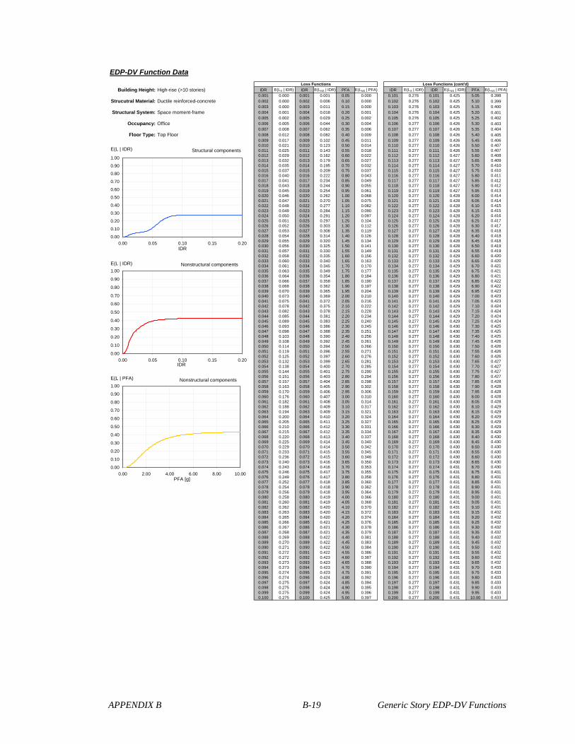
APPENDIX B B-19 Generic Story EDP-DV Functions
EDP-DV Function Data
Building Height: High-rise (>10 stories) IDR E(LS | IDR) IDR E(LNS | IDR) PFA E(LNS | PFA) IDR E(LS | IDR) IDR E(LNS | IDR) PFA E(LNS | PFA)
0.001 0.000 0.001 0.001 0.05 0.000 0.101 0.276 0.101 0.425 5.05 0.398
Strucutral Material: Ductile reinforced-concrete 0.002 0.000 0.002 0.006 0.10 0.000 0.102 0.276 0.102 0.425 5.10 0.3990.003 0.000 0.003 0.011 0.15 0.000 0.103 0.276 0.103 0.425 5.15 0.400
Structural System: Space moment-frame 0.004 0.001 0.004 0.018 0.20 0.001 0.104 0.276 0.104 0.425 5.20 0.4010.005 0.002 0.005 0.029 0.25 0.002 0.105 0.276 0.105 0.425 5.25 0.402
Occupancy: Office 0.006 0.005 0.006 0.044 0.30 0.004 0.106 0.277 0.106 0.426 5.30 0.4030.007 0.008 0.007 0.062 0.35 0.006 0.107 0.277 0.107 0.426 5.35 0.404
Floor Type: Top Floor 0.008 0.012 0.008 0.082 0.40 0.009 0.108 0.277 0.108 0.426 5.40 0.4050.009 0.017 0.009 0.102 0.45 0.011 0.109 0.277 0.109 0.426 5.45 0.4060.010 0.021 0.010 0.123 0.50 0.014 0.110 0.277 0.110 0.426 5.50 0.4070.011 0.025 0.011 0.143 0.55 0.018 0.111 0.277 0.111 0.426 5.55 0.4070.012 0.029 0.012 0.162 0.60 0.022 0.112 0.277 0.112 0.427 5.60 0.4080.013 0.032 0.013 0.179 0.65 0.027 0.113 0.277 0.113 0.427 5.65 0.4090.014 0.035 0.014 0.195 0.70 0.032 0.114 0.277 0.114 0.427 5.70 0.4100.015 0.037 0.015 0.209 0.75 0.037 0.115 0.277 0.115 0.427 5.75 0.4100.016 0.040 0.016 0.222 0.80 0.043 0.116 0.277 0.116 0.427 5.80 0.4110.017 0.041 0.017 0.234 0.85 0.049 0.117 0.277 0.117 0.427 5.85 0.4120.018 0.043 0.018 0.244 0.90 0.055 0.118 0.277 0.118 0.427 5.90 0.4120.019 0.045 0.019 0.254 0.95 0.061 0.119 0.277 0.119 0.427 5.95 0.4130.020 0.046 0.020 0.262 1.00 0.068 0.120 0.277 0.120 0.428 6.00 0.4140.021 0.047 0.021 0.270 1.05 0.075 0.121 0.277 0.121 0.428 6.05 0.4140.022 0.048 0.022 0.277 1.10 0.082 0.122 0.277 0.122 0.428 6.10 0.4150.023 0.049 0.023 0.284 1.15 0.090 0.123 0.277 0.123 0.428 6.15 0.4150.024 0.050 0.024 0.291 1.20 0.097 0.124 0.277 0.124 0.428 6.20 0.4160.025 0.051 0.025 0.297 1.25 0.104 0.125 0.277 0.125 0.428 6.25 0.4170.026 0.052 0.026 0.303 1.30 0.112 0.126 0.277 0.126 0.428 6.30 0.4170.027 0.053 0.027 0.308 1.35 0.119 0.127 0.277 0.127 0.428 6.35 0.4180.028 0.054 0.028 0.314 1.40 0.126 0.128 0.277 0.128 0.428 6.40 0.4180.029 0.055 0.029 0.320 1.45 0.134 0.129 0.277 0.129 0.428 6.45 0.4180.030 0.056 0.030 0.325 1.50 0.141 0.130 0.277 0.130 0.428 6.50 0.4190.031 0.057 0.031 0.330 1.55 0.149 0.131 0.277 0.131 0.429 6.55 0.4190.032 0.058 0.032 0.335 1.60 0.156 0.132 0.277 0.132 0.429 6.60 0.4200.033 0.060 0.033 0.340 1.65 0.163 0.133 0.277 0.133 0.429 6.65 0.4200.034 0.061 0.034 0.345 1.70 0.170 0.134 0.277 0.134 0.429 6.70 0.4210.035 0.063 0.035 0.349 1.75 0.177 0.135 0.277 0.135 0.429 6.75 0.4210.036 0.064 0.036 0.354 1.80 0.184 0.136 0.277 0.136 0.429 6.80 0.4210.037 0.066 0.037 0.358 1.85 0.190 0.137 0.277 0.137 0.429 6.85 0.4220.038 0.068 0.038 0.362 1.90 0.197 0.138 0.277 0.138 0.429 6.90 0.4220.039 0.070 0.039 0.365 1.95 0.204 0.139 0.277 0.139 0.429 6.95 0.4230.040 0.073 0.040 0.369 2.00 0.210 0.140 0.277 0.140 0.429 7.00 0.4230.041 0.075 0.041 0.372 2.05 0.216 0.141 0.277 0.141 0.429 7.05 0.4230.042 0.078 0.042 0.375 2.10 0.222 0.142 0.277 0.142 0.429 7.10 0.4240.043 0.082 0.043 0.378 2.15 0.228 0.143 0.277 0.143 0.429 7.15 0.4240.044 0.085 0.044 0.381 2.20 0.234 0.144 0.277 0.144 0.429 7.20 0.4240.045 0.089 0.045 0.383 2.25 0.240 0.145 0.277 0.145 0.429 7.25 0.4240.046 0.093 0.046 0.386 2.30 0.245 0.146 0.277 0.146 0.430 7.30 0.4250.047 0.098 0.047 0.388 2.35 0.251 0.147 0.277 0.147 0.430 7.35 0.4250.048 0.103 0.048 0.390 2.40 0.256 0.148 0.277 0.148 0.430 7.40 0.4250.049 0.108 0.049 0.392 2.45 0.261 0.149 0.277 0.149 0.430 7.45 0.4260.050 0.114 0.050 0.394 2.50 0.266 0.150 0.277 0.150 0.430 7.50 0.4260.051 0.119 0.051 0.396 2.55 0.271 0.151 0.277 0.151 0.430 7.55 0.4260.052 0.125 0.052 0.397 2.60 0.276 0.152 0.277 0.152 0.430 7.60 0.4260.053 0.132 0.053 0.399 2.65 0.281 0.153 0.277 0.153 0.430 7.65 0.4270.054 0.138 0.054 0.400 2.70 0.285 0.154 0.277 0.154 0.430 7.70 0.4270.055 0.144 0.055 0.401 2.75 0.290 0.155 0.277 0.155 0.430 7.75 0.4270.056 0.151 0.056 0.403 2.80 0.294 0.156 0.277 0.156 0.430 7.80 0.4270.057 0.157 0.057 0.404 2.85 0.298 0.157 0.277 0.157 0.430 7.85 0.4280.058 0.163 0.058 0.405 2.90 0.302 0.158 0.277 0.158 0.430 7.90 0.4280.059 0.170 0.059 0.406 2.95 0.306 0.159 0.277 0.159 0.430 7.95 0.4280.060 0.176 0.060 0.407 3.00 0.310 0.160 0.277 0.160 0.430 8.00 0.4280.061 0.182 0.061 0.408 3.05 0.314 0.161 0.277 0.161 0.430 8.05 0.4280.062 0.188 0.062 0.409 3.10 0.317 0.162 0.277 0.162 0.430 8.10 0.4290.063 0.194 0.063 0.409 3.15 0.321 0.163 0.277 0.163 0.430 8.15 0.4290.064 0.200 0.064 0.410 3.20 0.324 0.164 0.277 0.164 0.430 8.20 0.4290.065 0.205 0.065 0.411 3.25 0.327 0.165 0.277 0.165 0.430 8.25 0.4290.066 0.210 0.066 0.412 3.30 0.331 0.166 0.277 0.166 0.430 8.30 0.4290.067 0.215 0.067 0.412 3.35 0.334 0.167 0.277 0.167 0.430 8.35 0.4290.068 0.220 0.068 0.413 3.40 0.337 0.168 0.277 0.168 0.430 8.40 0.4300.069 0.225 0.069 0.414 3.45 0.340 0.169 0.277 0.169 0.430 8.45 0.4300.070 0.229 0.070 0.414 3.50 0.342 0.170 0.277 0.170 0.430 8.50 0.4300.071 0.233 0.071 0.415 3.55 0.345 0.171 0.277 0.171 0.430 8.55 0.4300.072 0.236 0.072 0.415 3.60 0.348 0.172 0.277 0.172 0.430 8.60 0.4300.073 0.240 0.073 0.416 3.65 0.350 0.173 0.277 0.173 0.430 8.65 0.4300.074 0.243 0.074 0.416 3.70 0.353 0.174 0.277 0.174 0.431 8.70 0.4300.075 0.246 0.075 0.417 3.75 0.355 0.175 0.277 0.175 0.431 8.75 0.4310.076 0.249 0.076 0.417 3.80 0.358 0.176 0.277 0.176 0.431 8.80 0.4310.077 0.252 0.077 0.418 3.85 0.360 0.177 0.277 0.177 0.431 8.85 0.4310.078 0.254 0.078 0.418 3.90 0.362 0.178 0.277 0.178 0.431 8.90 0.4310.079 0.256 0.079 0.418 3.95 0.364 0.179 0.277 0.179 0.431 8.95 0.4310.080 0.258 0.080 0.419 4.00 0.366 0.180 0.277 0.180 0.431 9.00 0.4310.081 0.260 0.081 0.419 4.05 0.368 0.181 0.277 0.181 0.431 9.05 0.4310.082 0.262 0.082 0.420 4.10 0.370 0.182 0.277 0.182 0.431 9.10 0.4310.083 0.263 0.083 0.420 4.15 0.372 0.183 0.277 0.183 0.431 9.15 0.4320.084 0.265 0.084 0.420 4.20 0.374 0.184 0.277 0.184 0.431 9.20 0.4320.085 0.266 0.085 0.421 4.25 0.376 0.185 0.277 0.185 0.431 9.25 0.4320.086 0.267 0.086 0.421 4.30 0.378 0.186 0.277 0.186 0.431 9.30 0.4320.087 0.268 0.087 0.421 4.35 0.379 0.187 0.277 0.187 0.431 9.35 0.4320.088 0.269 0.088 0.422 4.40 0.381 0.188 0.277 0.188 0.431 9.40 0.4320.089 0.270 0.089 0.422 4.45 0.383 0.189 0.277 0.189 0.431 9.45 0.4320.090 0.271 0.090 0.422 4.50 0.384 0.190 0.277 0.190 0.431 9.50 0.4320.091 0.272 0.091 0.422 4.55 0.386 0.191 0.277 0.191 0.431 9.55 0.4320.092 0.272 0.092 0.423 4.60 0.387 0.192 0.277 0.192 0.431 9.60 0.4320.093 0.273 0.093 0.423 4.65 0.388 0.193 0.277 0.193 0.431 9.65 0.4320.094 0.273 0.094 0.423 4.70 0.390 0.194 0.277 0.194 0.431 9.70 0.4330.095 0.274 0.095 0.423 4.75 0.391 0.195 0.277 0.195 0.431 9.75 0.4330.096 0.274 0.096 0.424 4.80 0.392 0.196 0.277 0.196 0.431 9.80 0.4330.097 0.275 0.097 0.424 4.85 0.394 0.197 0.277 0.197 0.431 9.85 0.4330.098 0.275 0.098 0.424 4.90 0.395 0.198 0.277 0.198 0.431 9.90 0.4330.099 0.275 0.099 0.424 4.95 0.396 0.199 0.277 0.199 0.431 9.95 0.4330.100 0.275 0.100 0.425 5.00 0.397 0.200 0.277 0.200 0.431 10.00 0.433
Loss Functions Loss Functions (cont'd)
Structural components
0.00
0.10
0.20
0.30
0.40
0.50
0.60
0.70
0.80
0.90
1.00
0.00 0.05 0.10 0.15 0.20IDR
E(L | IDR)
Nonstructural components
0.00
0.10
0.20
0.30
0.40
0.50
0.60
0.70
0.80
0.90
1.00
0.00 0.05 0.10 0.15 0.20IDR
E(L | IDR)
Nonstructural components
0.00
0.10
0.20
0.30
0.40
0.50
0.60
0.70
0.80
0.90
1.00
0.00 2.00 4.00 6.00 8.00 10.00PFA [g]
E(L | PFA)
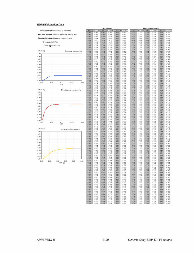
APPENDIX B B-20 Generic Story EDP-DV Functions
EDP-DV Function Data
Building Height: Low-rise (1 to 5 stories) IDR E(LS | IDR) IDR E(LNS | IDR) PFA E(LNS | PFA) IDR E(LS | IDR) IDR E(LNS | IDR) PFA E(LNS | PFA)
0.001 0.000 0.001 0.002 0.05 0.000 0.101 0.183 0.101 0.572 5.05 0.356
Strucutral Material: Non-ductile reinforced-concrete 0.002 0.000 0.002 0.009 0.10 0.000 0.102 0.183 0.102 0.572 5.10 0.3570.003 0.001 0.003 0.016 0.15 0.000 0.103 0.183 0.103 0.572 5.15 0.358
Structural System: Perimeter moment-frame 0.004 0.002 0.004 0.027 0.20 0.002 0.104 0.183 0.104 0.572 5.20 0.3580.005 0.004 0.005 0.044 0.25 0.004 0.105 0.183 0.105 0.573 5.25 0.359
Occupancy: Office 0.006 0.006 0.006 0.067 0.30 0.006 0.106 0.183 0.106 0.573 5.30 0.3600.007 0.010 0.007 0.094 0.35 0.009 0.107 0.183 0.107 0.573 5.35 0.361
Floor Type: 1st Floor 0.008 0.013 0.008 0.124 0.40 0.013 0.108 0.183 0.108 0.573 5.40 0.3610.009 0.018 0.009 0.154 0.45 0.016 0.109 0.183 0.109 0.573 5.45 0.3620.010 0.022 0.010 0.185 0.50 0.020 0.110 0.183 0.110 0.573 5.50 0.3630.011 0.027 0.011 0.213 0.55 0.024 0.111 0.183 0.111 0.573 5.55 0.3630.012 0.031 0.012 0.240 0.60 0.029 0.112 0.183 0.112 0.574 5.60 0.3640.013 0.035 0.013 0.265 0.65 0.034 0.113 0.183 0.113 0.574 5.65 0.3640.014 0.039 0.014 0.288 0.70 0.040 0.114 0.183 0.114 0.574 5.70 0.3650.015 0.043 0.015 0.308 0.75 0.045 0.115 0.183 0.115 0.574 5.75 0.3650.016 0.047 0.016 0.326 0.80 0.051 0.116 0.183 0.116 0.574 5.80 0.3660.017 0.051 0.017 0.342 0.85 0.057 0.117 0.183 0.117 0.574 5.85 0.3670.018 0.055 0.018 0.356 0.90 0.064 0.118 0.183 0.118 0.574 5.90 0.3670.019 0.059 0.019 0.369 0.95 0.070 0.119 0.183 0.119 0.574 5.95 0.3680.020 0.063 0.020 0.381 1.00 0.077 0.120 0.183 0.120 0.575 6.00 0.3680.021 0.068 0.021 0.391 1.05 0.084 0.121 0.183 0.121 0.575 6.05 0.3680.022 0.072 0.022 0.400 1.10 0.091 0.122 0.183 0.122 0.575 6.10 0.3690.023 0.077 0.023 0.409 1.15 0.098 0.123 0.183 0.123 0.575 6.15 0.3690.024 0.082 0.024 0.417 1.20 0.104 0.124 0.183 0.124 0.575 6.20 0.3700.025 0.088 0.025 0.425 1.25 0.111 0.125 0.183 0.125 0.575 6.25 0.3700.026 0.093 0.026 0.433 1.30 0.118 0.126 0.183 0.126 0.575 6.30 0.3710.027 0.099 0.027 0.440 1.35 0.125 0.127 0.183 0.127 0.575 6.35 0.3710.028 0.104 0.028 0.447 1.40 0.132 0.128 0.183 0.128 0.575 6.40 0.3710.029 0.110 0.029 0.453 1.45 0.138 0.129 0.183 0.129 0.575 6.45 0.3720.030 0.115 0.030 0.460 1.50 0.145 0.130 0.183 0.130 0.575 6.50 0.3720.031 0.120 0.031 0.466 1.55 0.151 0.131 0.183 0.131 0.575 6.55 0.3720.032 0.125 0.032 0.472 1.60 0.158 0.132 0.183 0.132 0.576 6.60 0.3730.033 0.130 0.033 0.478 1.65 0.164 0.133 0.183 0.133 0.576 6.65 0.3730.034 0.135 0.034 0.484 1.70 0.170 0.134 0.183 0.134 0.576 6.70 0.3730.035 0.140 0.035 0.489 1.75 0.176 0.135 0.183 0.135 0.576 6.75 0.3740.036 0.144 0.036 0.494 1.80 0.182 0.136 0.183 0.136 0.576 6.80 0.3740.037 0.148 0.037 0.499 1.85 0.188 0.137 0.183 0.137 0.576 6.85 0.3740.038 0.151 0.038 0.504 1.90 0.193 0.138 0.183 0.138 0.576 6.90 0.3750.039 0.155 0.039 0.508 1.95 0.199 0.139 0.183 0.139 0.576 6.95 0.3750.040 0.158 0.040 0.512 2.00 0.204 0.140 0.183 0.140 0.576 7.00 0.3750.041 0.161 0.041 0.516 2.05 0.209 0.141 0.183 0.141 0.576 7.05 0.3750.042 0.163 0.042 0.520 2.10 0.215 0.142 0.183 0.142 0.576 7.10 0.3760.043 0.165 0.043 0.523 2.15 0.220 0.143 0.183 0.143 0.576 7.15 0.3760.044 0.167 0.044 0.526 2.20 0.224 0.144 0.183 0.144 0.576 7.20 0.3760.045 0.169 0.045 0.529 2.25 0.229 0.145 0.183 0.145 0.576 7.25 0.3760.046 0.171 0.046 0.532 2.30 0.234 0.146 0.183 0.146 0.576 7.30 0.3770.047 0.172 0.047 0.534 2.35 0.238 0.147 0.183 0.147 0.576 7.35 0.3770.048 0.174 0.048 0.537 2.40 0.243 0.148 0.183 0.148 0.576 7.40 0.3770.049 0.175 0.049 0.539 2.45 0.247 0.149 0.183 0.149 0.577 7.45 0.3770.050 0.176 0.050 0.541 2.50 0.251 0.150 0.183 0.150 0.577 7.50 0.3770.051 0.177 0.051 0.543 2.55 0.255 0.151 0.183 0.151 0.577 7.55 0.3780.052 0.178 0.052 0.544 2.60 0.259 0.152 0.183 0.152 0.577 7.60 0.3780.053 0.178 0.053 0.546 2.65 0.263 0.153 0.183 0.153 0.577 7.65 0.3780.054 0.179 0.054 0.547 2.70 0.266 0.154 0.183 0.154 0.577 7.70 0.3780.055 0.179 0.055 0.549 2.75 0.270 0.155 0.183 0.155 0.577 7.75 0.3780.056 0.180 0.056 0.550 2.80 0.273 0.156 0.183 0.156 0.577 7.80 0.3790.057 0.180 0.057 0.551 2.85 0.277 0.157 0.183 0.157 0.577 7.85 0.3790.058 0.181 0.058 0.552 2.90 0.280 0.158 0.183 0.158 0.577 7.90 0.3790.059 0.181 0.059 0.553 2.95 0.283 0.159 0.183 0.159 0.577 7.95 0.3790.060 0.181 0.060 0.554 3.00 0.286 0.160 0.183 0.160 0.577 8.00 0.3790.061 0.182 0.061 0.555 3.05 0.289 0.161 0.183 0.161 0.577 8.05 0.3790.062 0.182 0.062 0.556 3.10 0.292 0.162 0.183 0.162 0.577 8.10 0.3790.063 0.182 0.063 0.557 3.15 0.295 0.163 0.183 0.163 0.577 8.15 0.3800.064 0.182 0.064 0.558 3.20 0.298 0.164 0.183 0.164 0.577 8.20 0.3800.065 0.182 0.065 0.559 3.25 0.300 0.165 0.183 0.165 0.577 8.25 0.3800.066 0.182 0.066 0.559 3.30 0.303 0.166 0.183 0.166 0.577 8.30 0.3800.067 0.182 0.067 0.560 3.35 0.305 0.167 0.183 0.167 0.577 8.35 0.3800.068 0.183 0.068 0.561 3.40 0.308 0.168 0.183 0.168 0.577 8.40 0.3800.069 0.183 0.069 0.561 3.45 0.310 0.169 0.183 0.169 0.577 8.45 0.3800.070 0.183 0.070 0.562 3.50 0.312 0.170 0.183 0.170 0.577 8.50 0.3810.071 0.183 0.071 0.562 3.55 0.314 0.171 0.183 0.171 0.577 8.55 0.3810.072 0.183 0.072 0.563 3.60 0.316 0.172 0.183 0.172 0.577 8.60 0.3810.073 0.183 0.073 0.563 3.65 0.319 0.173 0.183 0.173 0.577 8.65 0.3810.074 0.183 0.074 0.564 3.70 0.321 0.174 0.183 0.174 0.577 8.70 0.3810.075 0.183 0.075 0.564 3.75 0.322 0.175 0.183 0.175 0.577 8.75 0.3810.076 0.183 0.076 0.565 3.80 0.324 0.176 0.183 0.176 0.577 8.80 0.3810.077 0.183 0.077 0.565 3.85 0.326 0.177 0.183 0.177 0.577 8.85 0.3810.078 0.183 0.078 0.566 3.90 0.328 0.178 0.183 0.178 0.577 8.90 0.3810.079 0.183 0.079 0.566 3.95 0.330 0.179 0.183 0.179 0.577 8.95 0.3810.080 0.183 0.080 0.566 4.00 0.331 0.180 0.183 0.180 0.577 9.00 0.3820.081 0.183 0.081 0.567 4.05 0.333 0.181 0.183 0.181 0.577 9.05 0.3820.082 0.183 0.082 0.567 4.10 0.334 0.182 0.183 0.182 0.578 9.10 0.3820.083 0.183 0.083 0.567 4.15 0.336 0.183 0.183 0.183 0.578 9.15 0.3820.084 0.183 0.084 0.568 4.20 0.337 0.184 0.183 0.184 0.578 9.20 0.3820.085 0.183 0.085 0.568 4.25 0.339 0.185 0.183 0.185 0.578 9.25 0.3820.086 0.183 0.086 0.568 4.30 0.340 0.186 0.183 0.186 0.578 9.30 0.3820.087 0.183 0.087 0.569 4.35 0.341 0.187 0.183 0.187 0.578 9.35 0.3820.088 0.183 0.088 0.569 4.40 0.343 0.188 0.183 0.188 0.578 9.40 0.3820.089 0.183 0.089 0.569 4.45 0.344 0.189 0.183 0.189 0.578 9.45 0.3820.090 0.183 0.090 0.569 4.50 0.345 0.190 0.183 0.190 0.578 9.50 0.3820.091 0.183 0.091 0.570 4.55 0.346 0.191 0.183 0.191 0.578 9.55 0.3820.092 0.183 0.092 0.570 4.60 0.347 0.192 0.183 0.192 0.578 9.60 0.3820.093 0.183 0.093 0.570 4.65 0.348 0.193 0.183 0.193 0.578 9.65 0.3830.094 0.183 0.094 0.570 4.70 0.349 0.194 0.183 0.194 0.578 9.70 0.3830.095 0.183 0.095 0.571 4.75 0.350 0.195 0.183 0.195 0.578 9.75 0.3830.096 0.183 0.096 0.571 4.80 0.351 0.196 0.183 0.196 0.578 9.80 0.3830.097 0.183 0.097 0.571 4.85 0.352 0.197 0.183 0.197 0.578 9.85 0.3830.098 0.183 0.098 0.571 4.90 0.353 0.198 0.183 0.198 0.578 9.90 0.3830.099 0.183 0.099 0.571 4.95 0.354 0.199 0.183 0.199 0.578 9.95 0.3830.100 0.183 0.100 0.572 5.00 0.355 0.200 0.183 0.200 0.578 10.00 0.383
Loss Functions Loss Functions (cont'd)
Structural components
0.00
0.10
0.20
0.30
0.40
0.50
0.60
0.70
0.80
0.90
1.00
0.00 0.05 0.10 0.15 0.20IDR
E(L | IDR)
Nonstructural components
0.00
0.10
0.20
0.30
0.40
0.50
0.60
0.70
0.80
0.90
1.00
0.00 0.05 0.10 0.15 0.20IDR
E(L | IDR)
Nonstructural components
0.00
0.10
0.20
0.30
0.40
0.50
0.60
0.70
0.80
0.90
1.00
0.00 2.00 4.00 6.00 8.00 10.00PFA [g]
E(L | PFA)

APPENDIX B B-21 Generic Story EDP-DV Functions
EDP-DV Function Data
Building Height: Low-rise (1 to 5 stories) IDR E(LS | IDR) IDR E(LNS | IDR) PFA E(LNS | PFA) IDR E(LS | IDR) IDR E(LNS | IDR) PFA E(LNS | PFA)
0.001 0.000 0.001 0.002 0.05 0.000 0.101 0.189 0.101 0.540 5.05 0.374
Strucutral Material: Non-ductile reinforced-concrete 0.002 0.000 0.002 0.009 0.10 0.000 0.102 0.189 0.102 0.540 5.10 0.3750.003 0.001 0.003 0.015 0.15 0.001 0.103 0.189 0.103 0.540 5.15 0.376
Structural System: Perimeter moment-frame 0.004 0.002 0.004 0.026 0.20 0.002 0.104 0.189 0.104 0.540 5.20 0.3770.005 0.003 0.005 0.042 0.25 0.004 0.105 0.189 0.105 0.540 5.25 0.378
Occupancy: Office 0.006 0.005 0.006 0.064 0.30 0.007 0.106 0.189 0.106 0.540 5.30 0.3780.007 0.007 0.007 0.090 0.35 0.010 0.107 0.189 0.107 0.541 5.35 0.379
Floor Type: Typical Floor 0.008 0.010 0.008 0.119 0.40 0.014 0.108 0.189 0.108 0.541 5.40 0.3800.009 0.013 0.009 0.148 0.45 0.018 0.109 0.189 0.109 0.541 5.45 0.3800.010 0.016 0.010 0.177 0.50 0.022 0.110 0.189 0.110 0.541 5.50 0.3810.011 0.019 0.011 0.205 0.55 0.027 0.111 0.189 0.111 0.541 5.55 0.3820.012 0.022 0.012 0.231 0.60 0.032 0.112 0.189 0.112 0.541 5.60 0.3820.013 0.025 0.013 0.255 0.65 0.037 0.113 0.189 0.113 0.541 5.65 0.3830.014 0.028 0.014 0.276 0.70 0.043 0.114 0.189 0.114 0.542 5.70 0.3840.015 0.030 0.015 0.296 0.75 0.049 0.115 0.189 0.115 0.542 5.75 0.3840.016 0.033 0.016 0.313 0.80 0.055 0.116 0.189 0.116 0.542 5.80 0.3850.017 0.036 0.017 0.329 0.85 0.062 0.117 0.189 0.117 0.542 5.85 0.3850.018 0.039 0.018 0.342 0.90 0.069 0.118 0.189 0.118 0.542 5.90 0.3860.019 0.042 0.019 0.354 0.95 0.076 0.119 0.189 0.119 0.542 5.95 0.3860.020 0.045 0.020 0.365 1.00 0.083 0.120 0.189 0.120 0.542 6.00 0.3870.021 0.048 0.021 0.375 1.05 0.090 0.121 0.189 0.121 0.542 6.05 0.3870.022 0.051 0.022 0.384 1.10 0.097 0.122 0.189 0.122 0.542 6.10 0.3880.023 0.055 0.023 0.392 1.15 0.105 0.123 0.189 0.123 0.542 6.15 0.3880.024 0.058 0.024 0.400 1.20 0.112 0.124 0.189 0.124 0.543 6.20 0.3890.025 0.062 0.025 0.407 1.25 0.119 0.125 0.189 0.125 0.543 6.25 0.3890.026 0.066 0.026 0.414 1.30 0.126 0.126 0.189 0.126 0.543 6.30 0.3890.027 0.070 0.027 0.420 1.35 0.133 0.127 0.189 0.127 0.543 6.35 0.3900.028 0.074 0.028 0.427 1.40 0.140 0.128 0.189 0.128 0.543 6.40 0.3900.029 0.078 0.029 0.433 1.45 0.147 0.129 0.189 0.129 0.543 6.45 0.3910.030 0.082 0.030 0.439 1.50 0.154 0.130 0.189 0.130 0.543 6.50 0.3910.031 0.086 0.031 0.444 1.55 0.161 0.131 0.189 0.131 0.543 6.55 0.3910.032 0.089 0.032 0.450 1.60 0.168 0.132 0.189 0.132 0.543 6.60 0.3920.033 0.093 0.033 0.455 1.65 0.174 0.133 0.189 0.133 0.543 6.65 0.3920.034 0.097 0.034 0.460 1.70 0.181 0.134 0.189 0.134 0.543 6.70 0.3920.035 0.101 0.035 0.465 1.75 0.187 0.135 0.189 0.135 0.543 6.75 0.3930.036 0.105 0.036 0.470 1.80 0.193 0.136 0.189 0.136 0.543 6.80 0.3930.037 0.108 0.037 0.474 1.85 0.199 0.137 0.189 0.137 0.543 6.85 0.3930.038 0.112 0.038 0.478 1.90 0.205 0.138 0.189 0.138 0.543 6.90 0.3940.039 0.115 0.039 0.482 1.95 0.211 0.139 0.189 0.139 0.544 6.95 0.3940.040 0.118 0.040 0.486 2.00 0.217 0.140 0.189 0.140 0.544 7.00 0.3940.041 0.122 0.041 0.489 2.05 0.222 0.141 0.189 0.141 0.544 7.05 0.3940.042 0.125 0.042 0.492 2.10 0.227 0.142 0.189 0.142 0.544 7.10 0.3950.043 0.128 0.043 0.495 2.15 0.233 0.143 0.189 0.143 0.544 7.15 0.3950.044 0.131 0.044 0.498 2.20 0.238 0.144 0.189 0.144 0.544 7.20 0.3950.045 0.134 0.045 0.501 2.25 0.243 0.145 0.189 0.145 0.544 7.25 0.3950.046 0.137 0.046 0.503 2.30 0.247 0.146 0.189 0.146 0.544 7.30 0.3960.047 0.140 0.047 0.505 2.35 0.252 0.147 0.189 0.147 0.544 7.35 0.3960.048 0.144 0.048 0.507 2.40 0.257 0.148 0.189 0.148 0.544 7.40 0.3960.049 0.147 0.049 0.509 2.45 0.261 0.149 0.189 0.149 0.544 7.45 0.3960.050 0.150 0.050 0.511 2.50 0.265 0.150 0.189 0.150 0.544 7.50 0.3970.051 0.153 0.051 0.513 2.55 0.270 0.151 0.189 0.151 0.544 7.55 0.3970.052 0.155 0.052 0.514 2.60 0.274 0.152 0.189 0.152 0.544 7.60 0.3970.053 0.158 0.053 0.516 2.65 0.278 0.153 0.189 0.153 0.544 7.65 0.3970.054 0.161 0.054 0.517 2.70 0.281 0.154 0.189 0.154 0.544 7.70 0.3970.055 0.164 0.055 0.518 2.75 0.285 0.155 0.189 0.155 0.544 7.75 0.3980.056 0.166 0.056 0.519 2.80 0.289 0.156 0.189 0.156 0.544 7.80 0.3980.057 0.168 0.057 0.521 2.85 0.292 0.157 0.189 0.157 0.544 7.85 0.3980.058 0.171 0.058 0.522 2.90 0.296 0.158 0.189 0.158 0.544 7.90 0.3980.059 0.172 0.059 0.523 2.95 0.299 0.159 0.189 0.159 0.544 7.95 0.3980.060 0.174 0.060 0.523 3.00 0.302 0.160 0.189 0.160 0.544 8.00 0.3980.061 0.176 0.061 0.524 3.05 0.305 0.161 0.189 0.161 0.544 8.05 0.3980.062 0.178 0.062 0.525 3.10 0.308 0.162 0.189 0.162 0.544 8.10 0.3990.063 0.179 0.063 0.526 3.15 0.311 0.163 0.189 0.163 0.545 8.15 0.3990.064 0.180 0.064 0.527 3.20 0.314 0.164 0.189 0.164 0.545 8.20 0.3990.065 0.181 0.065 0.527 3.25 0.317 0.165 0.189 0.165 0.545 8.25 0.3990.066 0.182 0.066 0.528 3.30 0.319 0.166 0.189 0.166 0.545 8.30 0.3990.067 0.183 0.067 0.529 3.35 0.322 0.167 0.189 0.167 0.545 8.35 0.3990.068 0.184 0.068 0.529 3.40 0.324 0.168 0.189 0.168 0.545 8.40 0.3990.069 0.184 0.069 0.530 3.45 0.327 0.169 0.189 0.169 0.545 8.45 0.4000.070 0.185 0.070 0.530 3.50 0.329 0.170 0.189 0.170 0.545 8.50 0.4000.071 0.186 0.071 0.531 3.55 0.331 0.171 0.189 0.171 0.545 8.55 0.4000.072 0.186 0.072 0.531 3.60 0.333 0.172 0.189 0.172 0.545 8.60 0.4000.073 0.186 0.073 0.532 3.65 0.336 0.173 0.189 0.173 0.545 8.65 0.4000.074 0.187 0.074 0.532 3.70 0.338 0.174 0.189 0.174 0.545 8.70 0.4000.075 0.187 0.075 0.533 3.75 0.340 0.175 0.189 0.175 0.545 8.75 0.4000.076 0.187 0.076 0.533 3.80 0.341 0.176 0.189 0.176 0.545 8.80 0.4000.077 0.187 0.077 0.533 3.85 0.343 0.177 0.189 0.177 0.545 8.85 0.4000.078 0.188 0.078 0.534 3.90 0.345 0.178 0.189 0.178 0.545 8.90 0.4010.079 0.188 0.079 0.534 3.95 0.347 0.179 0.189 0.179 0.545 8.95 0.4010.080 0.188 0.080 0.534 4.00 0.349 0.180 0.189 0.180 0.545 9.00 0.4010.081 0.188 0.081 0.535 4.05 0.350 0.181 0.189 0.181 0.545 9.05 0.4010.082 0.188 0.082 0.535 4.10 0.352 0.182 0.189 0.182 0.545 9.10 0.4010.083 0.188 0.083 0.535 4.15 0.353 0.183 0.189 0.183 0.545 9.15 0.4010.084 0.188 0.084 0.536 4.20 0.355 0.184 0.189 0.184 0.545 9.20 0.4010.085 0.188 0.085 0.536 4.25 0.356 0.185 0.189 0.185 0.545 9.25 0.4010.086 0.188 0.086 0.536 4.30 0.358 0.186 0.189 0.186 0.545 9.30 0.4010.087 0.188 0.087 0.537 4.35 0.359 0.187 0.189 0.187 0.545 9.35 0.4010.088 0.189 0.088 0.537 4.40 0.360 0.188 0.189 0.188 0.545 9.40 0.4010.089 0.189 0.089 0.537 4.45 0.362 0.189 0.189 0.189 0.545 9.45 0.4020.090 0.189 0.090 0.537 4.50 0.363 0.190 0.189 0.190 0.545 9.50 0.4020.091 0.189 0.091 0.538 4.55 0.364 0.191 0.189 0.191 0.545 9.55 0.4020.092 0.189 0.092 0.538 4.60 0.365 0.192 0.189 0.192 0.545 9.60 0.4020.093 0.189 0.093 0.538 4.65 0.366 0.193 0.189 0.193 0.545 9.65 0.4020.094 0.189 0.094 0.538 4.70 0.368 0.194 0.189 0.194 0.545 9.70 0.4020.095 0.189 0.095 0.539 4.75 0.369 0.195 0.189 0.195 0.545 9.75 0.4020.096 0.189 0.096 0.539 4.80 0.370 0.196 0.189 0.196 0.545 9.80 0.4020.097 0.189 0.097 0.539 4.85 0.371 0.197 0.189 0.197 0.545 9.85 0.4020.098 0.189 0.098 0.539 4.90 0.372 0.198 0.189 0.198 0.545 9.90 0.4020.099 0.189 0.099 0.539 4.95 0.373 0.199 0.189 0.199 0.545 9.95 0.4020.100 0.189 0.100 0.539 5.00 0.373 0.200 0.189 0.200 0.545 10.00 0.402
Loss Functions Loss Functions (cont'd)
Structural components
0.00
0.10
0.20
0.30
0.40
0.50
0.60
0.70
0.80
0.90
1.00
0.00 0.05 0.10 0.15 0.20IDR
E(L | IDR)
Nonstructural components
0.00
0.10
0.20
0.30
0.40
0.50
0.60
0.70
0.80
0.90
1.00
0.00 0.05 0.10 0.15 0.20IDR
E(L | IDR)
Nonstructural components
0.00
0.10
0.20
0.30
0.40
0.50
0.60
0.70
0.80
0.90
1.00
0.00 2.00 4.00 6.00 8.00 10.00PFA [g]
E(L | PFA)

APPENDIX B B-22 Generic Story EDP-DV Functions
EDP-DV Function Data
Building Height: Low-rise (1 to 5 stories) IDR E(LS | IDR) IDR E(LNS | IDR) PFA E(LNS | PFA) IDR E(LS | IDR) IDR E(LNS | IDR) PFA E(LNS | PFA)
0.001 0.000 0.001 0.002 0.05 0.000 0.101 0.155 0.101 0.478 5.05 0.397
Strucutral Material: Non-ductile reinforced-concrete 0.002 0.000 0.002 0.007 0.10 0.000 0.102 0.155 0.102 0.479 5.10 0.3980.003 0.000 0.003 0.013 0.15 0.000 0.103 0.155 0.103 0.479 5.15 0.399
Structural System: Perimeter moment-frame 0.004 0.001 0.004 0.021 0.20 0.001 0.104 0.155 0.104 0.479 5.20 0.4000.005 0.003 0.005 0.034 0.25 0.003 0.105 0.155 0.105 0.479 5.25 0.401
Occupancy: Office 0.006 0.004 0.006 0.052 0.30 0.005 0.106 0.155 0.106 0.479 5.30 0.4020.007 0.006 0.007 0.074 0.35 0.007 0.107 0.155 0.107 0.479 5.35 0.403
Floor Type: Top Floor 0.008 0.008 0.008 0.097 0.40 0.010 0.108 0.155 0.108 0.480 5.40 0.4040.009 0.011 0.009 0.122 0.45 0.013 0.109 0.155 0.109 0.480 5.45 0.4040.010 0.013 0.010 0.146 0.50 0.016 0.110 0.155 0.110 0.480 5.50 0.4050.011 0.016 0.011 0.169 0.55 0.020 0.111 0.155 0.111 0.480 5.55 0.4060.012 0.018 0.012 0.191 0.60 0.024 0.112 0.155 0.112 0.480 5.60 0.4070.013 0.020 0.013 0.211 0.65 0.029 0.113 0.155 0.113 0.480 5.65 0.4070.014 0.023 0.014 0.230 0.70 0.034 0.114 0.155 0.114 0.480 5.70 0.4080.015 0.025 0.015 0.246 0.75 0.040 0.115 0.155 0.115 0.480 5.75 0.4090.016 0.027 0.016 0.261 0.80 0.046 0.116 0.155 0.116 0.481 5.80 0.4100.017 0.029 0.017 0.275 0.85 0.052 0.117 0.155 0.117 0.481 5.85 0.4100.018 0.032 0.018 0.287 0.90 0.059 0.118 0.156 0.118 0.481 5.90 0.4110.019 0.034 0.019 0.297 0.95 0.065 0.119 0.156 0.119 0.481 5.95 0.4110.020 0.037 0.020 0.307 1.00 0.072 0.120 0.156 0.120 0.481 6.00 0.4120.021 0.039 0.021 0.315 1.05 0.079 0.121 0.156 0.121 0.481 6.05 0.4130.022 0.042 0.022 0.324 1.10 0.086 0.122 0.156 0.122 0.481 6.10 0.4130.023 0.045 0.023 0.331 1.15 0.094 0.123 0.156 0.123 0.481 6.15 0.4140.024 0.048 0.024 0.338 1.20 0.101 0.124 0.156 0.124 0.481 6.20 0.4140.025 0.051 0.025 0.345 1.25 0.109 0.125 0.156 0.125 0.481 6.25 0.4150.026 0.054 0.026 0.351 1.30 0.116 0.126 0.156 0.126 0.482 6.30 0.4150.027 0.057 0.027 0.358 1.35 0.123 0.127 0.156 0.127 0.482 6.35 0.4160.028 0.060 0.028 0.364 1.40 0.131 0.128 0.156 0.128 0.482 6.40 0.4160.029 0.064 0.029 0.370 1.45 0.138 0.129 0.156 0.129 0.482 6.45 0.4170.030 0.067 0.030 0.376 1.50 0.146 0.130 0.156 0.130 0.482 6.50 0.4170.031 0.070 0.031 0.381 1.55 0.153 0.131 0.156 0.131 0.482 6.55 0.4180.032 0.074 0.032 0.387 1.60 0.160 0.132 0.156 0.132 0.482 6.60 0.4180.033 0.077 0.033 0.392 1.65 0.167 0.133 0.156 0.133 0.482 6.65 0.4180.034 0.080 0.034 0.397 1.70 0.174 0.134 0.156 0.134 0.482 6.70 0.4190.035 0.083 0.035 0.402 1.75 0.181 0.135 0.156 0.135 0.482 6.75 0.4190.036 0.086 0.036 0.406 1.80 0.188 0.136 0.156 0.136 0.482 6.80 0.4200.037 0.089 0.037 0.411 1.85 0.194 0.137 0.156 0.137 0.482 6.85 0.4200.038 0.092 0.038 0.415 1.90 0.201 0.138 0.156 0.138 0.482 6.90 0.4200.039 0.095 0.039 0.419 1.95 0.207 0.139 0.156 0.139 0.482 6.95 0.4210.040 0.097 0.040 0.423 2.00 0.214 0.140 0.156 0.140 0.483 7.00 0.4210.041 0.100 0.041 0.426 2.05 0.220 0.141 0.156 0.141 0.483 7.05 0.4210.042 0.103 0.042 0.429 2.10 0.226 0.142 0.156 0.142 0.483 7.10 0.4220.043 0.105 0.043 0.432 2.15 0.232 0.143 0.156 0.143 0.483 7.15 0.4220.044 0.108 0.044 0.435 2.20 0.237 0.144 0.156 0.144 0.483 7.20 0.4220.045 0.110 0.045 0.438 2.25 0.243 0.145 0.156 0.145 0.483 7.25 0.4220.046 0.113 0.046 0.440 2.30 0.248 0.146 0.156 0.146 0.483 7.30 0.4230.047 0.115 0.047 0.443 2.35 0.254 0.147 0.156 0.147 0.483 7.35 0.4230.048 0.118 0.048 0.445 2.40 0.259 0.148 0.156 0.148 0.483 7.40 0.4230.049 0.121 0.049 0.447 2.45 0.264 0.149 0.156 0.149 0.483 7.45 0.4240.050 0.123 0.050 0.449 2.50 0.269 0.150 0.156 0.150 0.483 7.50 0.4240.051 0.125 0.051 0.450 2.55 0.274 0.151 0.156 0.151 0.483 7.55 0.4240.052 0.128 0.052 0.452 2.60 0.278 0.152 0.156 0.152 0.483 7.60 0.4240.053 0.130 0.053 0.454 2.65 0.283 0.153 0.156 0.153 0.483 7.65 0.4250.054 0.132 0.054 0.455 2.70 0.287 0.154 0.156 0.154 0.483 7.70 0.4250.055 0.135 0.055 0.456 2.75 0.292 0.155 0.156 0.155 0.483 7.75 0.4250.056 0.137 0.056 0.457 2.80 0.296 0.156 0.156 0.156 0.483 7.80 0.4250.057 0.138 0.057 0.459 2.85 0.300 0.157 0.156 0.157 0.483 7.85 0.4250.058 0.140 0.058 0.460 2.90 0.304 0.158 0.156 0.158 0.483 7.90 0.4260.059 0.142 0.059 0.461 2.95 0.308 0.159 0.156 0.159 0.483 7.95 0.4260.060 0.143 0.060 0.462 3.00 0.311 0.160 0.156 0.160 0.483 8.00 0.4260.061 0.145 0.061 0.462 3.05 0.315 0.161 0.156 0.161 0.483 8.05 0.4260.062 0.146 0.062 0.463 3.10 0.318 0.162 0.156 0.162 0.483 8.10 0.4260.063 0.147 0.063 0.464 3.15 0.322 0.163 0.156 0.163 0.483 8.15 0.4270.064 0.148 0.064 0.465 3.20 0.325 0.164 0.156 0.164 0.484 8.20 0.4270.065 0.149 0.065 0.466 3.25 0.328 0.165 0.156 0.165 0.484 8.25 0.4270.066 0.150 0.066 0.466 3.30 0.331 0.166 0.156 0.166 0.484 8.30 0.4270.067 0.151 0.067 0.467 3.35 0.334 0.167 0.156 0.167 0.484 8.35 0.4270.068 0.151 0.068 0.467 3.40 0.337 0.168 0.156 0.168 0.484 8.40 0.4270.069 0.152 0.069 0.468 3.45 0.340 0.169 0.156 0.169 0.484 8.45 0.4280.070 0.152 0.070 0.469 3.50 0.343 0.170 0.156 0.170 0.484 8.50 0.4280.071 0.153 0.071 0.469 3.55 0.346 0.171 0.156 0.171 0.484 8.55 0.4280.072 0.153 0.072 0.470 3.60 0.348 0.172 0.156 0.172 0.484 8.60 0.4280.073 0.153 0.073 0.470 3.65 0.351 0.173 0.156 0.173 0.484 8.65 0.4280.074 0.154 0.074 0.471 3.70 0.353 0.174 0.156 0.174 0.484 8.70 0.4280.075 0.154 0.075 0.471 3.75 0.356 0.175 0.156 0.175 0.484 8.75 0.4280.076 0.154 0.076 0.471 3.80 0.358 0.176 0.156 0.176 0.484 8.80 0.4280.077 0.154 0.077 0.472 3.85 0.360 0.177 0.156 0.177 0.484 8.85 0.4290.078 0.154 0.078 0.472 3.90 0.362 0.178 0.156 0.178 0.484 8.90 0.4290.079 0.154 0.079 0.473 3.95 0.364 0.179 0.156 0.179 0.484 8.95 0.4290.080 0.155 0.080 0.473 4.00 0.366 0.180 0.156 0.180 0.484 9.00 0.4290.081 0.155 0.081 0.473 4.05 0.368 0.181 0.156 0.181 0.484 9.05 0.4290.082 0.155 0.082 0.474 4.10 0.370 0.182 0.156 0.182 0.484 9.10 0.4290.083 0.155 0.083 0.474 4.15 0.372 0.183 0.156 0.183 0.484 9.15 0.4290.084 0.155 0.084 0.474 4.20 0.374 0.184 0.156 0.184 0.484 9.20 0.4290.085 0.155 0.085 0.475 4.25 0.376 0.185 0.156 0.185 0.484 9.25 0.4290.086 0.155 0.086 0.475 4.30 0.377 0.186 0.156 0.186 0.484 9.30 0.4300.087 0.155 0.087 0.475 4.35 0.379 0.187 0.156 0.187 0.484 9.35 0.4300.088 0.155 0.088 0.476 4.40 0.380 0.188 0.156 0.188 0.484 9.40 0.4300.089 0.155 0.089 0.476 4.45 0.382 0.189 0.156 0.189 0.484 9.45 0.4300.090 0.155 0.090 0.476 4.50 0.383 0.190 0.156 0.190 0.484 9.50 0.4300.091 0.155 0.091 0.476 4.55 0.385 0.191 0.156 0.191 0.484 9.55 0.4300.092 0.155 0.092 0.477 4.60 0.386 0.192 0.156 0.192 0.484 9.60 0.4300.093 0.155 0.093 0.477 4.65 0.388 0.193 0.156 0.193 0.484 9.65 0.4300.094 0.155 0.094 0.477 4.70 0.389 0.194 0.156 0.194 0.484 9.70 0.4300.095 0.155 0.095 0.477 4.75 0.390 0.195 0.156 0.195 0.484 9.75 0.4300.096 0.155 0.096 0.477 4.80 0.391 0.196 0.156 0.196 0.484 9.80 0.4300.097 0.155 0.097 0.478 4.85 0.393 0.197 0.156 0.197 0.484 9.85 0.4310.098 0.155 0.098 0.478 4.90 0.394 0.198 0.156 0.198 0.484 9.90 0.4310.099 0.155 0.099 0.478 4.95 0.395 0.199 0.156 0.199 0.484 9.95 0.4310.100 0.155 0.100 0.478 5.00 0.396 0.200 0.156 0.200 0.484 10.00 0.431
Loss Functions Loss Functions (cont'd)
Structural components
0.00
0.10
0.20
0.30
0.40
0.50
0.60
0.70
0.80
0.90
1.00
0.00 0.05 0.10 0.15 0.20IDR
E(L | IDR)
Nonstructural components
0.00
0.10
0.20
0.30
0.40
0.50
0.60
0.70
0.80
0.90
1.00
0.00 0.05 0.10 0.15 0.20IDR
E(L | IDR)
Nonstructural components
0.00
0.10
0.20
0.30
0.40
0.50
0.60
0.70
0.80
0.90
1.00
0.00 2.00 4.00 6.00 8.00 10.00PFA [g]
E(L | PFA)

APPENDIX B B-23 Generic Story EDP-DV Functions
EDP-DV Function Data
Building Height: Mid-rise (5 to 10 stories) IDR E(LS | IDR) IDR E(LNS | IDR) PFA E(LNS | PFA) IDR E(LS | IDR) IDR E(LNS | IDR) PFA E(LNS | PFA)
0.001 0.000 0.001 0.002 0.05 0.000 0.101 0.267 0.101 0.521 5.05 0.352
Strucutral Material: Non-ductile reinforced-concrete 0.002 0.000 0.002 0.008 0.10 0.000 0.102 0.267 0.102 0.522 5.10 0.3520.003 0.001 0.003 0.015 0.15 0.000 0.103 0.267 0.103 0.522 5.15 0.353
Structural System: Perimeter moment-frame 0.004 0.003 0.004 0.024 0.20 0.002 0.104 0.267 0.104 0.522 5.20 0.3540.005 0.005 0.005 0.040 0.25 0.003 0.105 0.267 0.105 0.522 5.25 0.355
Occupancy: Office 0.006 0.009 0.006 0.060 0.30 0.006 0.106 0.267 0.106 0.522 5.30 0.3560.007 0.014 0.007 0.085 0.35 0.008 0.107 0.267 0.107 0.522 5.35 0.356
Floor Type: 1st Floor 0.008 0.020 0.008 0.112 0.40 0.011 0.108 0.267 0.108 0.522 5.40 0.3570.009 0.026 0.009 0.139 0.45 0.014 0.109 0.267 0.109 0.523 5.45 0.3580.010 0.033 0.010 0.166 0.50 0.018 0.110 0.267 0.110 0.523 5.50 0.3580.011 0.039 0.011 0.192 0.55 0.022 0.111 0.267 0.111 0.523 5.55 0.3590.012 0.046 0.012 0.216 0.60 0.026 0.112 0.267 0.112 0.523 5.60 0.3600.013 0.052 0.013 0.238 0.65 0.031 0.113 0.267 0.113 0.523 5.65 0.3600.014 0.057 0.014 0.258 0.70 0.036 0.114 0.267 0.114 0.523 5.70 0.3610.015 0.063 0.015 0.277 0.75 0.041 0.115 0.267 0.115 0.523 5.75 0.3610.016 0.069 0.016 0.293 0.80 0.047 0.116 0.267 0.116 0.523 5.80 0.3620.017 0.074 0.017 0.307 0.85 0.053 0.117 0.267 0.117 0.524 5.85 0.3620.018 0.080 0.018 0.320 0.90 0.059 0.118 0.267 0.118 0.524 5.90 0.3630.019 0.086 0.019 0.331 0.95 0.065 0.119 0.267 0.119 0.524 5.95 0.3640.020 0.092 0.020 0.342 1.00 0.071 0.120 0.267 0.120 0.524 6.00 0.3640.021 0.099 0.021 0.351 1.05 0.078 0.121 0.267 0.121 0.524 6.05 0.3640.022 0.106 0.022 0.360 1.10 0.084 0.122 0.267 0.122 0.524 6.10 0.3650.023 0.113 0.023 0.368 1.15 0.091 0.123 0.267 0.123 0.524 6.15 0.3650.024 0.120 0.024 0.375 1.20 0.098 0.124 0.267 0.124 0.524 6.20 0.3660.025 0.128 0.025 0.383 1.25 0.104 0.125 0.267 0.125 0.524 6.25 0.3660.026 0.136 0.026 0.389 1.30 0.111 0.126 0.267 0.126 0.524 6.30 0.3670.027 0.144 0.027 0.396 1.35 0.118 0.127 0.267 0.127 0.524 6.35 0.3670.028 0.152 0.028 0.403 1.40 0.124 0.128 0.267 0.128 0.525 6.40 0.3670.029 0.160 0.029 0.409 1.45 0.131 0.129 0.267 0.129 0.525 6.45 0.3680.030 0.168 0.030 0.415 1.50 0.137 0.130 0.267 0.130 0.525 6.50 0.3680.031 0.175 0.031 0.421 1.55 0.144 0.131 0.267 0.131 0.525 6.55 0.3690.032 0.183 0.032 0.427 1.60 0.150 0.132 0.267 0.132 0.525 6.60 0.3690.033 0.190 0.033 0.432 1.65 0.156 0.133 0.267 0.133 0.525 6.65 0.3690.034 0.197 0.034 0.438 1.70 0.162 0.134 0.267 0.134 0.525 6.70 0.3700.035 0.203 0.035 0.443 1.75 0.168 0.135 0.267 0.135 0.525 6.75 0.3700.036 0.210 0.036 0.448 1.80 0.174 0.136 0.267 0.136 0.525 6.80 0.3700.037 0.215 0.037 0.452 1.85 0.180 0.137 0.267 0.137 0.525 6.85 0.3710.038 0.221 0.038 0.457 1.90 0.186 0.138 0.267 0.138 0.525 6.90 0.3710.039 0.225 0.039 0.461 1.95 0.191 0.139 0.267 0.139 0.525 6.95 0.3710.040 0.230 0.040 0.465 2.00 0.197 0.140 0.267 0.140 0.525 7.00 0.3710.041 0.234 0.041 0.469 2.05 0.202 0.141 0.267 0.141 0.525 7.05 0.3720.042 0.238 0.042 0.472 2.10 0.207 0.142 0.267 0.142 0.525 7.10 0.3720.043 0.241 0.043 0.475 2.15 0.212 0.143 0.267 0.143 0.525 7.15 0.3720.044 0.244 0.044 0.478 2.20 0.217 0.144 0.267 0.144 0.525 7.20 0.3720.045 0.247 0.045 0.481 2.25 0.222 0.145 0.267 0.145 0.526 7.25 0.3730.046 0.249 0.046 0.484 2.30 0.227 0.146 0.267 0.146 0.526 7.30 0.3730.047 0.251 0.047 0.486 2.35 0.231 0.147 0.267 0.147 0.526 7.35 0.3730.048 0.253 0.048 0.488 2.40 0.236 0.148 0.267 0.148 0.526 7.40 0.3730.049 0.255 0.049 0.490 2.45 0.240 0.149 0.267 0.149 0.526 7.45 0.3740.050 0.256 0.050 0.492 2.50 0.244 0.150 0.267 0.150 0.526 7.50 0.3740.051 0.258 0.051 0.494 2.55 0.248 0.151 0.267 0.151 0.526 7.55 0.3740.052 0.259 0.052 0.495 2.60 0.252 0.152 0.267 0.152 0.526 7.60 0.3740.053 0.260 0.053 0.497 2.65 0.256 0.153 0.267 0.153 0.526 7.65 0.3740.054 0.261 0.054 0.498 2.70 0.260 0.154 0.267 0.154 0.526 7.70 0.3750.055 0.262 0.055 0.500 2.75 0.263 0.155 0.267 0.155 0.526 7.75 0.3750.056 0.262 0.056 0.501 2.80 0.267 0.156 0.267 0.156 0.526 7.80 0.3750.057 0.263 0.057 0.502 2.85 0.270 0.157 0.267 0.157 0.526 7.85 0.3750.058 0.263 0.058 0.503 2.90 0.274 0.158 0.267 0.158 0.526 7.90 0.3750.059 0.264 0.059 0.504 2.95 0.277 0.159 0.267 0.159 0.526 7.95 0.3750.060 0.264 0.060 0.505 3.00 0.280 0.160 0.267 0.160 0.526 8.00 0.3760.061 0.265 0.061 0.506 3.05 0.283 0.161 0.267 0.161 0.526 8.05 0.3760.062 0.265 0.062 0.507 3.10 0.286 0.162 0.267 0.162 0.526 8.10 0.3760.063 0.265 0.063 0.508 3.15 0.289 0.163 0.267 0.163 0.526 8.15 0.3760.064 0.265 0.064 0.508 3.20 0.292 0.164 0.267 0.164 0.526 8.20 0.3760.065 0.266 0.065 0.509 3.25 0.294 0.165 0.267 0.165 0.526 8.25 0.3760.066 0.266 0.066 0.510 3.30 0.297 0.166 0.267 0.166 0.526 8.30 0.3760.067 0.266 0.067 0.510 3.35 0.299 0.167 0.267 0.167 0.526 8.35 0.3770.068 0.266 0.068 0.511 3.40 0.302 0.168 0.267 0.168 0.526 8.40 0.3770.069 0.266 0.069 0.511 3.45 0.304 0.169 0.267 0.169 0.526 8.45 0.3770.070 0.266 0.070 0.512 3.50 0.307 0.170 0.267 0.170 0.526 8.50 0.3770.071 0.266 0.071 0.512 3.55 0.309 0.171 0.267 0.171 0.526 8.55 0.3770.072 0.266 0.072 0.513 3.60 0.311 0.172 0.267 0.172 0.526 8.60 0.3770.073 0.266 0.073 0.513 3.65 0.313 0.173 0.267 0.173 0.526 8.65 0.3770.074 0.266 0.074 0.514 3.70 0.315 0.174 0.267 0.174 0.526 8.70 0.3770.075 0.266 0.075 0.514 3.75 0.317 0.175 0.267 0.175 0.526 8.75 0.3780.076 0.267 0.076 0.515 3.80 0.319 0.176 0.267 0.176 0.527 8.80 0.3780.077 0.267 0.077 0.515 3.85 0.321 0.177 0.267 0.177 0.527 8.85 0.3780.078 0.267 0.078 0.515 3.90 0.323 0.178 0.267 0.178 0.527 8.90 0.3780.079 0.267 0.079 0.516 3.95 0.324 0.179 0.267 0.179 0.527 8.95 0.3780.080 0.267 0.080 0.516 4.00 0.326 0.180 0.267 0.180 0.527 9.00 0.3780.081 0.267 0.081 0.517 4.05 0.328 0.181 0.267 0.181 0.527 9.05 0.3780.082 0.267 0.082 0.517 4.10 0.329 0.182 0.267 0.182 0.527 9.10 0.3780.083 0.267 0.083 0.517 4.15 0.331 0.183 0.267 0.183 0.527 9.15 0.3780.084 0.267 0.084 0.517 4.20 0.332 0.184 0.267 0.184 0.527 9.20 0.3780.085 0.267 0.085 0.518 4.25 0.334 0.185 0.267 0.185 0.527 9.25 0.3780.086 0.267 0.086 0.518 4.30 0.335 0.186 0.267 0.186 0.527 9.30 0.3790.087 0.267 0.087 0.518 4.35 0.336 0.187 0.267 0.187 0.527 9.35 0.3790.088 0.267 0.088 0.519 4.40 0.338 0.188 0.267 0.188 0.527 9.40 0.3790.089 0.267 0.089 0.519 4.45 0.339 0.189 0.267 0.189 0.527 9.45 0.3790.090 0.267 0.090 0.519 4.50 0.340 0.190 0.267 0.190 0.527 9.50 0.3790.091 0.267 0.091 0.519 4.55 0.341 0.191 0.267 0.191 0.527 9.55 0.3790.092 0.267 0.092 0.520 4.60 0.343 0.192 0.267 0.192 0.527 9.60 0.3790.093 0.267 0.093 0.520 4.65 0.344 0.193 0.267 0.193 0.527 9.65 0.3790.094 0.267 0.094 0.520 4.70 0.345 0.194 0.267 0.194 0.527 9.70 0.3790.095 0.267 0.095 0.520 4.75 0.346 0.195 0.267 0.195 0.527 9.75 0.3790.096 0.267 0.096 0.520 4.80 0.347 0.196 0.267 0.196 0.527 9.80 0.3790.097 0.267 0.097 0.521 4.85 0.348 0.197 0.267 0.197 0.527 9.85 0.3790.098 0.267 0.098 0.521 4.90 0.349 0.198 0.267 0.198 0.527 9.90 0.3790.099 0.267 0.099 0.521 4.95 0.350 0.199 0.267 0.199 0.527 9.95 0.3790.100 0.267 0.100 0.521 5.00 0.351 0.200 0.267 0.200 0.527 10.00 0.379
Loss Functions Loss Functions (cont'd)
Structural components
0.00
0.10
0.20
0.30
0.40
0.50
0.60
0.70
0.80
0.90
1.00
0.00 0.05 0.10 0.15 0.20IDR
E(L | IDR)
Nonstructural components
0.00
0.10
0.20
0.30
0.40
0.50
0.60
0.70
0.80
0.90
1.00
0.00 0.05 0.10 0.15 0.20IDR
E(L | IDR)
Nonstructural components
0.00
0.10
0.20
0.30
0.40
0.50
0.60
0.70
0.80
0.90
1.00
0.00 2.00 4.00 6.00 8.00 10.00PFA [g]
E(L | PFA)

APPENDIX B B-24 Generic Story EDP-DV Functions
EDP-DV Function Data
Building Height: Mid-rise (5 to 10 stories) IDR E(LS | IDR) IDR E(LNS | IDR) PFA E(LNS | PFA) IDR E(LS | IDR) IDR E(LNS | IDR) PFA E(LNS | PFA)
0.001 0.000 0.001 0.002 0.05 0.000 0.101 0.275 0.101 0.488 5.05 0.368
Strucutral Material: Non-ductile reinforced-concrete 0.002 0.000 0.002 0.008 0.10 0.000 0.102 0.275 0.102 0.488 5.10 0.3690.003 0.001 0.003 0.014 0.15 0.000 0.103 0.275 0.103 0.489 5.15 0.370
Structural System: Perimeter moment-frame 0.004 0.002 0.004 0.023 0.20 0.002 0.104 0.275 0.104 0.489 5.20 0.3710.005 0.005 0.005 0.037 0.25 0.004 0.105 0.275 0.105 0.489 5.25 0.371
Occupancy: Office 0.006 0.007 0.006 0.057 0.30 0.006 0.106 0.275 0.106 0.489 5.30 0.3720.007 0.011 0.007 0.080 0.35 0.009 0.107 0.275 0.107 0.489 5.35 0.373
Floor Type: Typ Floor 0.008 0.015 0.008 0.105 0.40 0.012 0.108 0.275 0.108 0.489 5.40 0.3740.009 0.019 0.009 0.131 0.45 0.015 0.109 0.275 0.109 0.489 5.45 0.3740.010 0.023 0.010 0.157 0.50 0.019 0.110 0.275 0.110 0.490 5.50 0.3750.011 0.028 0.011 0.181 0.55 0.023 0.111 0.275 0.111 0.490 5.55 0.3760.012 0.032 0.012 0.204 0.60 0.028 0.112 0.275 0.112 0.490 5.60 0.3760.013 0.036 0.013 0.226 0.65 0.033 0.113 0.275 0.113 0.490 5.65 0.3770.014 0.040 0.014 0.245 0.70 0.038 0.114 0.275 0.114 0.490 5.70 0.3780.015 0.044 0.015 0.262 0.75 0.044 0.115 0.275 0.115 0.490 5.75 0.3780.016 0.048 0.016 0.278 0.80 0.050 0.116 0.275 0.116 0.490 5.80 0.3790.017 0.052 0.017 0.291 0.85 0.056 0.117 0.275 0.117 0.490 5.85 0.3790.018 0.056 0.018 0.304 0.90 0.063 0.118 0.275 0.118 0.490 5.90 0.3800.019 0.060 0.019 0.314 0.95 0.069 0.119 0.275 0.119 0.490 5.95 0.3800.020 0.065 0.020 0.324 1.00 0.076 0.120 0.275 0.120 0.491 6.00 0.3810.021 0.070 0.021 0.333 1.05 0.083 0.121 0.275 0.121 0.491 6.05 0.3810.022 0.074 0.022 0.341 1.10 0.090 0.122 0.275 0.122 0.491 6.10 0.3820.023 0.080 0.023 0.349 1.15 0.097 0.123 0.275 0.123 0.491 6.15 0.3820.024 0.085 0.024 0.356 1.20 0.104 0.124 0.275 0.124 0.491 6.20 0.3830.025 0.090 0.025 0.362 1.25 0.111 0.125 0.275 0.125 0.491 6.25 0.3830.026 0.096 0.026 0.369 1.30 0.118 0.126 0.275 0.126 0.491 6.30 0.3840.027 0.101 0.027 0.375 1.35 0.125 0.127 0.275 0.127 0.491 6.35 0.3840.028 0.107 0.028 0.381 1.40 0.132 0.128 0.275 0.128 0.491 6.40 0.3850.029 0.113 0.029 0.386 1.45 0.139 0.129 0.275 0.129 0.491 6.45 0.3850.030 0.119 0.030 0.392 1.50 0.146 0.130 0.275 0.130 0.491 6.50 0.3850.031 0.125 0.031 0.397 1.55 0.152 0.131 0.275 0.131 0.491 6.55 0.3860.032 0.130 0.032 0.402 1.60 0.159 0.132 0.275 0.132 0.491 6.60 0.3860.033 0.136 0.033 0.407 1.65 0.165 0.133 0.275 0.133 0.492 6.65 0.3860.034 0.142 0.034 0.412 1.70 0.172 0.134 0.275 0.134 0.492 6.70 0.3870.035 0.147 0.035 0.417 1.75 0.178 0.135 0.275 0.135 0.492 6.75 0.3870.036 0.152 0.036 0.421 1.80 0.184 0.136 0.275 0.136 0.492 6.80 0.3870.037 0.157 0.037 0.425 1.85 0.190 0.137 0.275 0.137 0.492 6.85 0.3880.038 0.163 0.038 0.429 1.90 0.196 0.138 0.275 0.138 0.492 6.90 0.3880.039 0.167 0.039 0.433 1.95 0.202 0.139 0.275 0.139 0.492 6.95 0.3880.040 0.172 0.040 0.437 2.00 0.207 0.140 0.275 0.140 0.492 7.00 0.3890.041 0.177 0.041 0.440 2.05 0.213 0.141 0.275 0.141 0.492 7.05 0.3890.042 0.182 0.042 0.443 2.10 0.218 0.142 0.275 0.142 0.492 7.10 0.3890.043 0.186 0.043 0.446 2.15 0.224 0.143 0.275 0.143 0.492 7.15 0.3890.044 0.191 0.044 0.448 2.20 0.229 0.144 0.275 0.144 0.492 7.20 0.3900.045 0.195 0.045 0.451 2.25 0.234 0.145 0.275 0.145 0.492 7.25 0.3900.046 0.200 0.046 0.453 2.30 0.239 0.146 0.275 0.146 0.492 7.30 0.3900.047 0.204 0.047 0.455 2.35 0.243 0.147 0.275 0.147 0.492 7.35 0.3900.048 0.209 0.048 0.457 2.40 0.248 0.148 0.275 0.148 0.492 7.40 0.3910.049 0.213 0.049 0.459 2.45 0.252 0.149 0.275 0.149 0.492 7.45 0.3910.050 0.218 0.050 0.461 2.50 0.257 0.150 0.275 0.150 0.492 7.50 0.3910.051 0.222 0.051 0.463 2.55 0.261 0.151 0.275 0.151 0.492 7.55 0.3910.052 0.226 0.052 0.464 2.60 0.265 0.152 0.275 0.152 0.492 7.60 0.3910.053 0.230 0.053 0.465 2.65 0.269 0.153 0.275 0.153 0.492 7.65 0.3920.054 0.234 0.054 0.467 2.70 0.273 0.154 0.275 0.154 0.493 7.70 0.3920.055 0.238 0.055 0.468 2.75 0.277 0.155 0.275 0.155 0.493 7.75 0.3920.056 0.242 0.056 0.469 2.80 0.280 0.156 0.275 0.156 0.493 7.80 0.3920.057 0.245 0.057 0.470 2.85 0.284 0.157 0.275 0.157 0.493 7.85 0.3920.058 0.248 0.058 0.471 2.90 0.287 0.158 0.275 0.158 0.493 7.90 0.3930.059 0.251 0.059 0.472 2.95 0.291 0.159 0.275 0.159 0.493 7.95 0.3930.060 0.254 0.060 0.473 3.00 0.294 0.160 0.275 0.160 0.493 8.00 0.3930.061 0.256 0.061 0.474 3.05 0.297 0.161 0.275 0.161 0.493 8.05 0.3930.062 0.259 0.062 0.474 3.10 0.300 0.162 0.275 0.162 0.493 8.10 0.3930.063 0.261 0.063 0.475 3.15 0.303 0.163 0.275 0.163 0.493 8.15 0.3930.064 0.262 0.064 0.476 3.20 0.306 0.164 0.275 0.164 0.493 8.20 0.3930.065 0.264 0.065 0.476 3.25 0.309 0.165 0.275 0.165 0.493 8.25 0.3940.066 0.265 0.066 0.477 3.30 0.311 0.166 0.275 0.166 0.493 8.30 0.3940.067 0.267 0.067 0.478 3.35 0.314 0.167 0.275 0.167 0.493 8.35 0.3940.068 0.268 0.068 0.478 3.40 0.317 0.168 0.275 0.168 0.493 8.40 0.3940.069 0.269 0.069 0.479 3.45 0.319 0.169 0.275 0.169 0.493 8.45 0.3940.070 0.269 0.070 0.479 3.50 0.321 0.170 0.276 0.170 0.493 8.50 0.3940.071 0.270 0.071 0.480 3.55 0.324 0.171 0.276 0.171 0.493 8.55 0.3940.072 0.271 0.072 0.480 3.60 0.326 0.172 0.276 0.172 0.493 8.60 0.3950.073 0.271 0.073 0.481 3.65 0.328 0.173 0.276 0.173 0.493 8.65 0.3950.074 0.272 0.074 0.481 3.70 0.330 0.174 0.276 0.174 0.493 8.70 0.3950.075 0.272 0.075 0.481 3.75 0.332 0.175 0.276 0.175 0.493 8.75 0.3950.076 0.273 0.076 0.482 3.80 0.334 0.176 0.276 0.176 0.493 8.80 0.3950.077 0.273 0.077 0.482 3.85 0.336 0.177 0.276 0.177 0.493 8.85 0.3950.078 0.273 0.078 0.483 3.90 0.338 0.178 0.276 0.178 0.493 8.90 0.3950.079 0.273 0.079 0.483 3.95 0.340 0.179 0.276 0.179 0.493 8.95 0.3950.080 0.274 0.080 0.483 4.00 0.342 0.180 0.276 0.180 0.493 9.00 0.3950.081 0.274 0.081 0.484 4.05 0.343 0.181 0.276 0.181 0.493 9.05 0.3950.082 0.274 0.082 0.484 4.10 0.345 0.182 0.276 0.182 0.493 9.10 0.3960.083 0.274 0.083 0.484 4.15 0.347 0.183 0.276 0.183 0.493 9.15 0.3960.084 0.274 0.084 0.485 4.20 0.348 0.184 0.276 0.184 0.493 9.20 0.3960.085 0.274 0.085 0.485 4.25 0.350 0.185 0.276 0.185 0.493 9.25 0.3960.086 0.274 0.086 0.485 4.30 0.351 0.186 0.276 0.186 0.493 9.30 0.3960.087 0.274 0.087 0.485 4.35 0.352 0.187 0.276 0.187 0.493 9.35 0.3960.088 0.275 0.088 0.486 4.40 0.354 0.188 0.276 0.188 0.493 9.40 0.3960.089 0.275 0.089 0.486 4.45 0.355 0.189 0.276 0.189 0.493 9.45 0.3960.090 0.275 0.090 0.486 4.50 0.356 0.190 0.276 0.190 0.493 9.50 0.3960.091 0.275 0.091 0.486 4.55 0.358 0.191 0.276 0.191 0.493 9.55 0.3960.092 0.275 0.092 0.487 4.60 0.359 0.192 0.276 0.192 0.493 9.60 0.3960.093 0.275 0.093 0.487 4.65 0.360 0.193 0.276 0.193 0.493 9.65 0.3960.094 0.275 0.094 0.487 4.70 0.361 0.194 0.276 0.194 0.493 9.70 0.3970.095 0.275 0.095 0.487 4.75 0.362 0.195 0.276 0.195 0.493 9.75 0.3970.096 0.275 0.096 0.487 4.80 0.363 0.196 0.276 0.196 0.493 9.80 0.3970.097 0.275 0.097 0.488 4.85 0.364 0.197 0.276 0.197 0.493 9.85 0.3970.098 0.275 0.098 0.488 4.90 0.365 0.198 0.276 0.198 0.493 9.90 0.3970.099 0.275 0.099 0.488 4.95 0.366 0.199 0.276 0.199 0.493 9.95 0.3970.100 0.275 0.100 0.488 5.00 0.367 0.200 0.276 0.200 0.493 10.00 0.397
Loss Functions Loss Functions (cont'd)
Structural components
0.00
0.10
0.20
0.30
0.40
0.50
0.60
0.70
0.80
0.90
1.00
0.00 0.05 0.10 0.15 0.20IDR
E(L | IDR)
Nonstructural components
0.00
0.10
0.20
0.30
0.40
0.50
0.60
0.70
0.80
0.90
1.00
0.00 0.05 0.10 0.15 0.20IDR
E(L | IDR)
Nonstructural components
0.00
0.10
0.20
0.30
0.40
0.50
0.60
0.70
0.80
0.90
1.00
0.00 2.00 4.00 6.00 8.00 10.00PFA [g]
E(L | PFA)

APPENDIX B B-25 Generic Story EDP-DV Functions
EDP-DV Function Data
Building Height: Mid-rise (5 to 10 stories) IDR E(LS | IDR) IDR E(LNS | IDR) PFA E(LNS | PFA) IDR E(LS | IDR) IDR E(LNS | IDR) PFA E(LNS | PFA)
0.001 0.000 0.001 0.001 0.05 0.000 0.101 0.229 0.101 0.453 5.05 0.404
Strucutral Material: Non-ductile reinforced-concrete 0.002 0.000 0.002 0.006 0.10 0.000 0.102 0.229 0.102 0.453 5.10 0.4050.003 0.001 0.003 0.012 0.15 0.000 0.103 0.229 0.103 0.453 5.15 0.406
Structural System: Perimeter moment-frame 0.004 0.002 0.004 0.020 0.20 0.001 0.104 0.229 0.104 0.453 5.20 0.4070.005 0.004 0.005 0.032 0.25 0.003 0.105 0.229 0.105 0.453 5.25 0.408
Occupancy: Office 0.006 0.006 0.006 0.049 0.30 0.004 0.106 0.229 0.106 0.454 5.30 0.4090.007 0.009 0.007 0.069 0.35 0.007 0.107 0.229 0.107 0.454 5.35 0.410
Floor Type: Top Floor 0.008 0.012 0.008 0.091 0.40 0.009 0.108 0.229 0.108 0.454 5.40 0.4110.009 0.016 0.009 0.114 0.45 0.012 0.109 0.229 0.109 0.454 5.45 0.4110.010 0.020 0.010 0.136 0.50 0.015 0.110 0.229 0.110 0.454 5.50 0.4120.011 0.023 0.011 0.158 0.55 0.019 0.111 0.229 0.111 0.454 5.55 0.4130.012 0.027 0.012 0.178 0.60 0.023 0.112 0.229 0.112 0.454 5.60 0.4140.013 0.030 0.013 0.197 0.65 0.028 0.113 0.229 0.113 0.454 5.65 0.4150.014 0.033 0.014 0.214 0.70 0.033 0.114 0.229 0.114 0.455 5.70 0.4150.015 0.037 0.015 0.230 0.75 0.038 0.115 0.229 0.115 0.455 5.75 0.4160.016 0.040 0.016 0.244 0.80 0.044 0.116 0.229 0.116 0.455 5.80 0.4170.017 0.043 0.017 0.256 0.85 0.050 0.117 0.229 0.117 0.455 5.85 0.4180.018 0.047 0.018 0.267 0.90 0.057 0.118 0.229 0.118 0.455 5.90 0.4180.019 0.050 0.019 0.277 0.95 0.064 0.119 0.229 0.119 0.455 5.95 0.4190.020 0.054 0.020 0.286 1.00 0.071 0.120 0.229 0.120 0.455 6.00 0.4190.021 0.058 0.021 0.294 1.05 0.078 0.121 0.229 0.121 0.455 6.05 0.4200.022 0.062 0.022 0.302 1.10 0.085 0.122 0.229 0.122 0.455 6.10 0.4210.023 0.066 0.023 0.309 1.15 0.092 0.123 0.230 0.123 0.456 6.15 0.4210.024 0.071 0.024 0.316 1.20 0.100 0.124 0.230 0.124 0.456 6.20 0.4220.025 0.075 0.025 0.322 1.25 0.107 0.125 0.230 0.125 0.456 6.25 0.4220.026 0.080 0.026 0.328 1.30 0.115 0.126 0.230 0.126 0.456 6.30 0.4230.027 0.084 0.027 0.335 1.35 0.122 0.127 0.230 0.127 0.456 6.35 0.4230.028 0.089 0.028 0.340 1.40 0.130 0.128 0.230 0.128 0.456 6.40 0.4240.029 0.094 0.029 0.346 1.45 0.137 0.129 0.230 0.129 0.456 6.45 0.4240.030 0.099 0.030 0.352 1.50 0.145 0.130 0.230 0.130 0.456 6.50 0.4250.031 0.104 0.031 0.357 1.55 0.152 0.131 0.230 0.131 0.456 6.55 0.4250.032 0.109 0.032 0.363 1.60 0.160 0.132 0.230 0.132 0.456 6.60 0.4260.033 0.113 0.033 0.368 1.65 0.167 0.133 0.230 0.133 0.456 6.65 0.4260.034 0.118 0.034 0.373 1.70 0.174 0.134 0.230 0.134 0.456 6.70 0.4260.035 0.122 0.035 0.377 1.75 0.181 0.135 0.230 0.135 0.456 6.75 0.4270.036 0.127 0.036 0.382 1.80 0.188 0.136 0.230 0.136 0.456 6.80 0.4270.037 0.131 0.037 0.386 1.85 0.195 0.137 0.230 0.137 0.457 6.85 0.4280.038 0.135 0.038 0.390 1.90 0.201 0.138 0.230 0.138 0.457 6.90 0.4280.039 0.140 0.039 0.394 1.95 0.208 0.139 0.230 0.139 0.457 6.95 0.4280.040 0.144 0.040 0.398 2.00 0.214 0.140 0.230 0.140 0.457 7.00 0.4290.041 0.148 0.041 0.401 2.05 0.221 0.141 0.230 0.141 0.457 7.05 0.4290.042 0.151 0.042 0.405 2.10 0.227 0.142 0.230 0.142 0.457 7.10 0.4290.043 0.155 0.043 0.408 2.15 0.233 0.143 0.230 0.143 0.457 7.15 0.4300.044 0.159 0.044 0.410 2.20 0.239 0.144 0.230 0.144 0.457 7.20 0.4300.045 0.163 0.045 0.413 2.25 0.244 0.145 0.230 0.145 0.457 7.25 0.4300.046 0.167 0.046 0.415 2.30 0.250 0.146 0.230 0.146 0.457 7.30 0.4310.047 0.170 0.047 0.418 2.35 0.256 0.147 0.230 0.147 0.457 7.35 0.4310.048 0.174 0.048 0.420 2.40 0.261 0.148 0.230 0.148 0.457 7.40 0.4310.049 0.178 0.049 0.422 2.45 0.266 0.149 0.230 0.149 0.457 7.45 0.4310.050 0.182 0.050 0.424 2.50 0.271 0.150 0.230 0.150 0.457 7.50 0.4320.051 0.185 0.051 0.425 2.55 0.276 0.151 0.230 0.151 0.457 7.55 0.4320.052 0.189 0.052 0.427 2.60 0.281 0.152 0.230 0.152 0.457 7.60 0.4320.053 0.192 0.053 0.428 2.65 0.286 0.153 0.230 0.153 0.457 7.65 0.4320.054 0.195 0.054 0.430 2.70 0.290 0.154 0.230 0.154 0.457 7.70 0.4330.055 0.199 0.055 0.431 2.75 0.295 0.155 0.230 0.155 0.457 7.75 0.4330.056 0.202 0.056 0.432 2.80 0.299 0.156 0.230 0.156 0.457 7.80 0.4330.057 0.204 0.057 0.433 2.85 0.303 0.157 0.230 0.157 0.457 7.85 0.4330.058 0.207 0.058 0.434 2.90 0.307 0.158 0.230 0.158 0.457 7.90 0.4340.059 0.209 0.059 0.435 2.95 0.311 0.159 0.230 0.159 0.458 7.95 0.4340.060 0.212 0.060 0.436 3.00 0.315 0.160 0.230 0.160 0.458 8.00 0.4340.061 0.214 0.061 0.437 3.05 0.319 0.161 0.230 0.161 0.458 8.05 0.4340.062 0.215 0.062 0.438 3.10 0.322 0.162 0.230 0.162 0.458 8.10 0.4340.063 0.217 0.063 0.439 3.15 0.326 0.163 0.230 0.163 0.458 8.15 0.4350.064 0.219 0.064 0.439 3.20 0.329 0.164 0.230 0.164 0.458 8.20 0.4350.065 0.220 0.065 0.440 3.25 0.333 0.165 0.230 0.165 0.458 8.25 0.4350.066 0.221 0.066 0.441 3.30 0.336 0.166 0.230 0.166 0.458 8.30 0.4350.067 0.222 0.067 0.441 3.35 0.339 0.167 0.230 0.167 0.458 8.35 0.4350.068 0.223 0.068 0.442 3.40 0.342 0.168 0.230 0.168 0.458 8.40 0.4350.069 0.224 0.069 0.443 3.45 0.345 0.169 0.230 0.169 0.458 8.45 0.4360.070 0.225 0.070 0.443 3.50 0.348 0.170 0.230 0.170 0.458 8.50 0.4360.071 0.225 0.071 0.444 3.55 0.351 0.171 0.230 0.171 0.458 8.55 0.4360.072 0.226 0.072 0.444 3.60 0.353 0.172 0.230 0.172 0.458 8.60 0.4360.073 0.226 0.073 0.445 3.65 0.356 0.173 0.230 0.173 0.458 8.65 0.4360.074 0.227 0.074 0.445 3.70 0.358 0.174 0.230 0.174 0.458 8.70 0.4360.075 0.227 0.075 0.445 3.75 0.361 0.175 0.230 0.175 0.458 8.75 0.4360.076 0.227 0.076 0.446 3.80 0.363 0.176 0.230 0.176 0.458 8.80 0.4370.077 0.227 0.077 0.446 3.85 0.365 0.177 0.230 0.177 0.458 8.85 0.4370.078 0.228 0.078 0.447 3.90 0.368 0.178 0.230 0.178 0.458 8.90 0.4370.079 0.228 0.079 0.447 3.95 0.370 0.179 0.230 0.179 0.458 8.95 0.4370.080 0.228 0.080 0.447 4.00 0.372 0.180 0.230 0.180 0.458 9.00 0.4370.081 0.228 0.081 0.448 4.05 0.374 0.181 0.230 0.181 0.458 9.05 0.4370.082 0.228 0.082 0.448 4.10 0.376 0.182 0.230 0.182 0.458 9.10 0.4370.083 0.228 0.083 0.448 4.15 0.378 0.183 0.230 0.183 0.458 9.15 0.4370.084 0.229 0.084 0.449 4.20 0.380 0.184 0.230 0.184 0.458 9.20 0.4370.085 0.229 0.085 0.449 4.25 0.382 0.185 0.230 0.185 0.458 9.25 0.4380.086 0.229 0.086 0.449 4.30 0.383 0.186 0.230 0.186 0.458 9.30 0.4380.087 0.229 0.087 0.450 4.35 0.385 0.187 0.230 0.187 0.458 9.35 0.4380.088 0.229 0.088 0.450 4.40 0.387 0.188 0.230 0.188 0.458 9.40 0.4380.089 0.229 0.089 0.450 4.45 0.388 0.189 0.230 0.189 0.458 9.45 0.4380.090 0.229 0.090 0.450 4.50 0.390 0.190 0.230 0.190 0.458 9.50 0.4380.091 0.229 0.091 0.451 4.55 0.391 0.191 0.230 0.191 0.458 9.55 0.4380.092 0.229 0.092 0.451 4.60 0.393 0.192 0.230 0.192 0.458 9.60 0.4380.093 0.229 0.093 0.451 4.65 0.394 0.193 0.230 0.193 0.458 9.65 0.4380.094 0.229 0.094 0.451 4.70 0.395 0.194 0.230 0.194 0.458 9.70 0.4380.095 0.229 0.095 0.452 4.75 0.397 0.195 0.230 0.195 0.458 9.75 0.4380.096 0.229 0.096 0.452 4.80 0.398 0.196 0.230 0.196 0.458 9.80 0.4390.097 0.229 0.097 0.452 4.85 0.399 0.197 0.230 0.197 0.458 9.85 0.4390.098 0.229 0.098 0.452 4.90 0.400 0.198 0.230 0.198 0.458 9.90 0.4390.099 0.229 0.099 0.452 4.95 0.402 0.199 0.230 0.199 0.458 9.95 0.4390.100 0.229 0.100 0.453 5.00 0.403 0.200 0.230 0.200 0.458 10.00 0.439
Loss Functions Loss Functions (cont'd)
Structural components
0.00
0.10
0.20
0.30
0.40
0.50
0.60
0.70
0.80
0.90
1.00
0.00 0.05 0.10 0.15 0.20IDR
E(L | IDR)
Nonstructural components
0.00
0.10
0.20
0.30
0.40
0.50
0.60
0.70
0.80
0.90
1.00
0.00 0.05 0.10 0.15 0.20IDR
E(L | IDR)
Nonstructural components
0.00
0.10
0.20
0.30
0.40
0.50
0.60
0.70
0.80
0.90
1.00
0.00 2.00 4.00 6.00 8.00 10.00PFA [g]
E(L | PFA)

APPENDIX B B-26 Generic Story EDP-DV Functions
EDP-DV Function Data
Building Height: High-rise (>10 stories) IDR E(LS | IDR) IDR E(LNS | IDR) PFA E(LNS | PFA) IDR E(LS | IDR) IDR E(LNS | IDR) PFA E(LNS | PFA)
0.001 0.000 0.001 0.002 0.05 0.000 0.101 0.343 0.101 0.479 5.05 0.342
Strucutral Material: Non-ductile reinforced-concrete 0.002 0.000 0.002 0.007 0.10 0.000 0.102 0.343 0.102 0.479 5.10 0.3430.003 0.001 0.003 0.013 0.15 0.000 0.103 0.343 0.103 0.479 5.15 0.344
Structural System: Perimeter moment-frame 0.004 0.003 0.004 0.022 0.20 0.001 0.104 0.343 0.104 0.479 5.20 0.3450.005 0.007 0.005 0.035 0.25 0.003 0.105 0.343 0.105 0.479 5.25 0.345
Occupancy: Office 0.006 0.012 0.006 0.054 0.30 0.005 0.106 0.343 0.106 0.479 5.30 0.3460.007 0.018 0.007 0.076 0.35 0.007 0.107 0.343 0.107 0.479 5.35 0.347
Floor Type: 1st Floor 0.008 0.025 0.008 0.099 0.40 0.010 0.108 0.343 0.108 0.480 5.40 0.3480.009 0.033 0.009 0.124 0.45 0.013 0.109 0.343 0.109 0.480 5.45 0.3480.010 0.042 0.010 0.148 0.50 0.016 0.110 0.343 0.110 0.480 5.50 0.3490.011 0.050 0.011 0.172 0.55 0.020 0.111 0.343 0.111 0.480 5.55 0.3500.012 0.059 0.012 0.194 0.60 0.024 0.112 0.343 0.112 0.480 5.60 0.3500.013 0.066 0.013 0.214 0.65 0.028 0.113 0.343 0.113 0.480 5.65 0.3510.014 0.074 0.014 0.232 0.70 0.033 0.114 0.343 0.114 0.480 5.70 0.3510.015 0.081 0.015 0.249 0.75 0.038 0.115 0.343 0.115 0.481 5.75 0.3520.016 0.088 0.016 0.264 0.80 0.044 0.116 0.343 0.116 0.481 5.80 0.3530.017 0.096 0.017 0.277 0.85 0.049 0.117 0.343 0.117 0.481 5.85 0.3530.018 0.103 0.018 0.289 0.90 0.055 0.118 0.343 0.118 0.481 5.90 0.3540.019 0.111 0.019 0.299 0.95 0.061 0.119 0.343 0.119 0.481 5.95 0.3540.020 0.119 0.020 0.309 1.00 0.067 0.120 0.343 0.120 0.481 6.00 0.3550.021 0.127 0.021 0.317 1.05 0.074 0.121 0.343 0.121 0.481 6.05 0.3550.022 0.136 0.022 0.325 1.10 0.080 0.122 0.343 0.122 0.481 6.10 0.3560.023 0.145 0.023 0.333 1.15 0.086 0.123 0.343 0.123 0.481 6.15 0.3560.024 0.154 0.024 0.340 1.20 0.093 0.124 0.343 0.124 0.481 6.20 0.3560.025 0.164 0.025 0.347 1.25 0.099 0.125 0.343 0.125 0.482 6.25 0.3570.026 0.174 0.026 0.353 1.30 0.106 0.126 0.343 0.126 0.482 6.30 0.3570.027 0.185 0.027 0.359 1.35 0.112 0.127 0.343 0.127 0.482 6.35 0.3580.028 0.195 0.028 0.365 1.40 0.119 0.128 0.343 0.128 0.482 6.40 0.3580.029 0.205 0.029 0.371 1.45 0.125 0.129 0.343 0.129 0.482 6.45 0.3580.030 0.215 0.030 0.377 1.50 0.131 0.130 0.343 0.130 0.482 6.50 0.3590.031 0.225 0.031 0.382 1.55 0.137 0.131 0.343 0.131 0.482 6.55 0.3590.032 0.235 0.032 0.388 1.60 0.144 0.132 0.343 0.132 0.482 6.60 0.3600.033 0.244 0.033 0.393 1.65 0.150 0.133 0.343 0.133 0.482 6.65 0.3600.034 0.253 0.034 0.398 1.70 0.156 0.134 0.343 0.134 0.482 6.70 0.3600.035 0.262 0.035 0.403 1.75 0.162 0.135 0.343 0.135 0.482 6.75 0.3600.036 0.269 0.036 0.407 1.80 0.167 0.136 0.343 0.136 0.482 6.80 0.3610.037 0.277 0.037 0.411 1.85 0.173 0.137 0.343 0.137 0.482 6.85 0.3610.038 0.284 0.038 0.416 1.90 0.178 0.138 0.343 0.138 0.483 6.90 0.3610.039 0.290 0.039 0.419 1.95 0.184 0.139 0.343 0.139 0.483 6.95 0.3620.040 0.296 0.040 0.423 2.00 0.189 0.140 0.343 0.140 0.483 7.00 0.3620.041 0.301 0.041 0.427 2.05 0.194 0.141 0.343 0.141 0.483 7.05 0.3620.042 0.306 0.042 0.430 2.10 0.199 0.142 0.343 0.142 0.483 7.10 0.3620.043 0.310 0.043 0.433 2.15 0.204 0.143 0.343 0.143 0.483 7.15 0.3630.044 0.314 0.044 0.436 2.20 0.209 0.144 0.343 0.144 0.483 7.20 0.3630.045 0.317 0.045 0.438 2.25 0.214 0.145 0.343 0.145 0.483 7.25 0.3630.046 0.320 0.046 0.441 2.30 0.219 0.146 0.343 0.146 0.483 7.30 0.3630.047 0.323 0.047 0.443 2.35 0.223 0.147 0.343 0.147 0.483 7.35 0.3640.048 0.326 0.048 0.445 2.40 0.227 0.148 0.343 0.148 0.483 7.40 0.3640.049 0.328 0.049 0.447 2.45 0.232 0.149 0.343 0.149 0.483 7.45 0.3640.050 0.330 0.050 0.449 2.50 0.236 0.150 0.343 0.150 0.483 7.50 0.3640.051 0.331 0.051 0.451 2.55 0.240 0.151 0.343 0.151 0.483 7.55 0.3650.052 0.333 0.052 0.452 2.60 0.244 0.152 0.343 0.152 0.483 7.60 0.3650.053 0.334 0.053 0.454 2.65 0.248 0.153 0.343 0.153 0.483 7.65 0.3650.054 0.335 0.054 0.455 2.70 0.251 0.154 0.343 0.154 0.483 7.70 0.3650.055 0.336 0.055 0.456 2.75 0.255 0.155 0.343 0.155 0.483 7.75 0.3650.056 0.337 0.056 0.458 2.80 0.258 0.156 0.343 0.156 0.483 7.80 0.3650.057 0.338 0.057 0.459 2.85 0.262 0.157 0.343 0.157 0.483 7.85 0.3660.058 0.339 0.058 0.460 2.90 0.265 0.158 0.343 0.158 0.483 7.90 0.3660.059 0.339 0.059 0.461 2.95 0.268 0.159 0.343 0.159 0.483 7.95 0.3660.060 0.340 0.060 0.462 3.00 0.271 0.160 0.343 0.160 0.483 8.00 0.3660.061 0.340 0.061 0.463 3.05 0.274 0.161 0.343 0.161 0.484 8.05 0.3660.062 0.341 0.062 0.463 3.10 0.277 0.162 0.343 0.162 0.484 8.10 0.3660.063 0.341 0.063 0.464 3.15 0.280 0.163 0.343 0.163 0.484 8.15 0.3670.064 0.341 0.064 0.465 3.20 0.283 0.164 0.343 0.164 0.484 8.20 0.3670.065 0.341 0.065 0.466 3.25 0.285 0.165 0.343 0.165 0.484 8.25 0.3670.066 0.342 0.066 0.466 3.30 0.288 0.166 0.343 0.166 0.484 8.30 0.3670.067 0.342 0.067 0.467 3.35 0.290 0.167 0.343 0.167 0.484 8.35 0.3670.068 0.342 0.068 0.468 3.40 0.293 0.168 0.343 0.168 0.484 8.40 0.3670.069 0.342 0.069 0.468 3.45 0.295 0.169 0.343 0.169 0.484 8.45 0.3670.070 0.342 0.070 0.469 3.50 0.298 0.170 0.343 0.170 0.484 8.50 0.3670.071 0.342 0.071 0.469 3.55 0.300 0.171 0.343 0.171 0.484 8.55 0.3680.072 0.342 0.072 0.470 3.60 0.302 0.172 0.343 0.172 0.484 8.60 0.3680.073 0.343 0.073 0.470 3.65 0.304 0.173 0.343 0.173 0.484 8.65 0.3680.074 0.343 0.074 0.471 3.70 0.306 0.174 0.343 0.174 0.484 8.70 0.3680.075 0.343 0.075 0.471 3.75 0.308 0.175 0.343 0.175 0.484 8.75 0.3680.076 0.343 0.076 0.472 3.80 0.310 0.176 0.343 0.176 0.484 8.80 0.3680.077 0.343 0.077 0.472 3.85 0.312 0.177 0.343 0.177 0.484 8.85 0.3680.078 0.343 0.078 0.472 3.90 0.313 0.178 0.343 0.178 0.484 8.90 0.3680.079 0.343 0.079 0.473 3.95 0.315 0.179 0.343 0.179 0.484 8.95 0.3680.080 0.343 0.080 0.473 4.00 0.317 0.180 0.343 0.180 0.484 9.00 0.3690.081 0.343 0.081 0.473 4.05 0.318 0.181 0.343 0.181 0.484 9.05 0.3690.082 0.343 0.082 0.474 4.10 0.320 0.182 0.343 0.182 0.484 9.10 0.3690.083 0.343 0.083 0.474 4.15 0.322 0.183 0.343 0.183 0.484 9.15 0.3690.084 0.343 0.084 0.474 4.20 0.323 0.184 0.343 0.184 0.484 9.20 0.3690.085 0.343 0.085 0.475 4.25 0.324 0.185 0.343 0.185 0.484 9.25 0.3690.086 0.343 0.086 0.475 4.30 0.326 0.186 0.343 0.186 0.484 9.30 0.3690.087 0.343 0.087 0.475 4.35 0.327 0.187 0.343 0.187 0.484 9.35 0.3690.088 0.343 0.088 0.476 4.40 0.329 0.188 0.343 0.188 0.484 9.40 0.3690.089 0.343 0.089 0.476 4.45 0.330 0.189 0.343 0.189 0.484 9.45 0.3690.090 0.343 0.090 0.476 4.50 0.331 0.190 0.343 0.190 0.484 9.50 0.3690.091 0.343 0.091 0.476 4.55 0.332 0.191 0.343 0.191 0.484 9.55 0.3690.092 0.343 0.092 0.477 4.60 0.333 0.192 0.343 0.192 0.484 9.60 0.3700.093 0.343 0.093 0.477 4.65 0.334 0.193 0.343 0.193 0.484 9.65 0.3700.094 0.343 0.094 0.477 4.70 0.336 0.194 0.343 0.194 0.484 9.70 0.3700.095 0.343 0.095 0.477 4.75 0.337 0.195 0.343 0.195 0.484 9.75 0.3700.096 0.343 0.096 0.478 4.80 0.338 0.196 0.343 0.196 0.484 9.80 0.3700.097 0.343 0.097 0.478 4.85 0.339 0.197 0.343 0.197 0.484 9.85 0.3700.098 0.343 0.098 0.478 4.90 0.340 0.198 0.343 0.198 0.484 9.90 0.3700.099 0.343 0.099 0.478 4.95 0.340 0.199 0.343 0.199 0.484 9.95 0.3700.100 0.343 0.100 0.478 5.00 0.341 0.200 0.343 0.200 0.484 10.00 0.370
Loss Functions Loss Functions (cont'd)
Structural components
0.00
0.10
0.20
0.30
0.40
0.50
0.60
0.70
0.80
0.90
1.00
0.00 0.05 0.10 0.15 0.20IDR
E(L | IDR)
Nonstructural components
0.00
0.10
0.20
0.30
0.40
0.50
0.60
0.70
0.80
0.90
1.00
0.00 0.05 0.10 0.15 0.20IDR
E(L | IDR)
Nonstructural components
0.00
0.10
0.20
0.30
0.40
0.50
0.60
0.70
0.80
0.90
1.00
0.00 2.00 4.00 6.00 8.00 10.00PFA [g]
E(L | PFA)

APPENDIX B B-27 Generic Story EDP-DV Functions
EDP-DV Function Data
Building Height: High-rise (>10 stories) IDR E(LS | IDR) IDR E(LNS | IDR) PFA E(LNS | PFA) IDR E(LS | IDR) IDR E(LNS | IDR) PFA E(LNS | PFA)
0.001 0.000 0.001 0.002 0.05 0.000 0.101 0.352 0.101 0.448 5.05 0.356
Strucutral Material: Non-ductile reinforced-concrete 0.002 0.000 0.002 0.007 0.10 0.000 0.102 0.352 0.102 0.448 5.10 0.3570.003 0.001 0.003 0.012 0.15 0.000 0.103 0.352 0.103 0.448 5.15 0.358
Structural System: Perimeter moment-frame 0.004 0.003 0.004 0.020 0.20 0.001 0.104 0.352 0.104 0.449 5.20 0.3590.005 0.006 0.005 0.033 0.25 0.003 0.105 0.352 0.105 0.449 5.25 0.360
Occupancy: Office 0.006 0.009 0.006 0.050 0.30 0.005 0.106 0.352 0.106 0.449 5.30 0.3600.007 0.014 0.007 0.071 0.35 0.008 0.107 0.353 0.107 0.449 5.35 0.361
Floor Type: Typ Floor 0.008 0.019 0.008 0.093 0.40 0.011 0.108 0.353 0.108 0.449 5.40 0.3620.009 0.024 0.009 0.116 0.45 0.014 0.109 0.353 0.109 0.449 5.45 0.3630.010 0.030 0.010 0.140 0.50 0.018 0.110 0.353 0.110 0.449 5.50 0.3630.011 0.036 0.011 0.162 0.55 0.021 0.111 0.353 0.111 0.450 5.55 0.3640.012 0.041 0.012 0.183 0.60 0.026 0.112 0.353 0.112 0.450 5.60 0.3650.013 0.046 0.013 0.202 0.65 0.030 0.113 0.353 0.113 0.450 5.65 0.3650.014 0.051 0.014 0.219 0.70 0.035 0.114 0.353 0.114 0.450 5.70 0.3660.015 0.056 0.015 0.235 0.75 0.041 0.115 0.353 0.115 0.450 5.75 0.3660.016 0.061 0.016 0.249 0.80 0.046 0.116 0.353 0.116 0.450 5.80 0.3670.017 0.067 0.017 0.262 0.85 0.052 0.117 0.353 0.117 0.450 5.85 0.3680.018 0.072 0.018 0.273 0.90 0.059 0.118 0.353 0.118 0.450 5.90 0.3680.019 0.077 0.019 0.283 0.95 0.065 0.119 0.353 0.119 0.451 5.95 0.3690.020 0.083 0.020 0.292 1.00 0.071 0.120 0.353 0.120 0.451 6.00 0.3690.021 0.089 0.021 0.300 1.05 0.078 0.121 0.353 0.121 0.451 6.05 0.3700.022 0.095 0.022 0.308 1.10 0.085 0.122 0.353 0.122 0.451 6.10 0.3700.023 0.102 0.023 0.315 1.15 0.091 0.123 0.353 0.123 0.451 6.15 0.3710.024 0.109 0.024 0.321 1.20 0.098 0.124 0.353 0.124 0.451 6.20 0.3710.025 0.116 0.025 0.328 1.25 0.105 0.125 0.353 0.125 0.451 6.25 0.3710.026 0.123 0.026 0.334 1.30 0.111 0.126 0.353 0.126 0.451 6.30 0.3720.027 0.130 0.027 0.339 1.35 0.118 0.127 0.353 0.127 0.451 6.35 0.3720.028 0.137 0.028 0.345 1.40 0.125 0.128 0.353 0.128 0.451 6.40 0.3730.029 0.145 0.029 0.350 1.45 0.132 0.129 0.353 0.129 0.451 6.45 0.3730.030 0.152 0.030 0.355 1.50 0.138 0.130 0.353 0.130 0.451 6.50 0.3730.031 0.160 0.031 0.360 1.55 0.145 0.131 0.353 0.131 0.452 6.55 0.3740.032 0.167 0.032 0.365 1.60 0.151 0.132 0.353 0.132 0.452 6.60 0.3740.033 0.174 0.033 0.370 1.65 0.157 0.133 0.353 0.133 0.452 6.65 0.3740.034 0.181 0.034 0.374 1.70 0.163 0.134 0.353 0.134 0.452 6.70 0.3750.035 0.188 0.035 0.379 1.75 0.170 0.135 0.353 0.135 0.452 6.75 0.3750.036 0.195 0.036 0.383 1.80 0.176 0.136 0.353 0.136 0.452 6.80 0.3750.037 0.202 0.037 0.387 1.85 0.181 0.137 0.353 0.137 0.452 6.85 0.3760.038 0.208 0.038 0.390 1.90 0.187 0.138 0.353 0.138 0.452 6.90 0.3760.039 0.214 0.039 0.394 1.95 0.193 0.139 0.353 0.139 0.452 6.95 0.3760.040 0.221 0.040 0.397 2.00 0.198 0.140 0.353 0.140 0.452 7.00 0.3770.041 0.227 0.041 0.400 2.05 0.204 0.141 0.353 0.141 0.452 7.05 0.3770.042 0.233 0.042 0.403 2.10 0.209 0.142 0.353 0.142 0.452 7.10 0.3770.043 0.239 0.043 0.406 2.15 0.214 0.143 0.353 0.143 0.452 7.15 0.3770.044 0.244 0.044 0.408 2.20 0.219 0.144 0.353 0.144 0.452 7.20 0.3780.045 0.250 0.045 0.411 2.25 0.224 0.145 0.353 0.145 0.452 7.25 0.3780.046 0.256 0.046 0.413 2.30 0.229 0.146 0.353 0.146 0.452 7.30 0.3780.047 0.262 0.047 0.415 2.35 0.233 0.147 0.353 0.147 0.452 7.35 0.3780.048 0.268 0.048 0.417 2.40 0.238 0.148 0.353 0.148 0.452 7.40 0.3790.049 0.273 0.049 0.419 2.45 0.242 0.149 0.353 0.149 0.453 7.45 0.3790.050 0.279 0.050 0.420 2.50 0.247 0.150 0.353 0.150 0.453 7.50 0.3790.051 0.285 0.051 0.422 2.55 0.251 0.151 0.353 0.151 0.453 7.55 0.3790.052 0.290 0.052 0.423 2.60 0.255 0.152 0.353 0.152 0.453 7.60 0.3790.053 0.295 0.053 0.425 2.65 0.259 0.153 0.353 0.153 0.453 7.65 0.3800.054 0.300 0.054 0.426 2.70 0.262 0.154 0.353 0.154 0.453 7.70 0.3800.055 0.305 0.055 0.427 2.75 0.266 0.155 0.353 0.155 0.453 7.75 0.3800.056 0.310 0.056 0.428 2.80 0.270 0.156 0.353 0.156 0.453 7.80 0.3800.057 0.314 0.057 0.429 2.85 0.273 0.157 0.353 0.157 0.453 7.85 0.3800.058 0.318 0.058 0.430 2.90 0.277 0.158 0.353 0.158 0.453 7.90 0.3810.059 0.322 0.059 0.431 2.95 0.280 0.159 0.353 0.159 0.453 7.95 0.3810.060 0.325 0.060 0.432 3.00 0.283 0.160 0.353 0.160 0.453 8.00 0.3810.061 0.328 0.061 0.433 3.05 0.286 0.161 0.353 0.161 0.453 8.05 0.3810.062 0.331 0.062 0.434 3.10 0.289 0.162 0.353 0.162 0.453 8.10 0.3810.063 0.334 0.063 0.434 3.15 0.292 0.163 0.353 0.163 0.453 8.15 0.3810.064 0.336 0.064 0.435 3.20 0.295 0.164 0.353 0.164 0.453 8.20 0.3820.065 0.338 0.065 0.436 3.25 0.298 0.165 0.353 0.165 0.453 8.25 0.3820.066 0.340 0.066 0.436 3.30 0.300 0.166 0.353 0.166 0.453 8.30 0.3820.067 0.341 0.067 0.437 3.35 0.303 0.167 0.353 0.167 0.453 8.35 0.3820.068 0.343 0.068 0.438 3.40 0.306 0.168 0.353 0.168 0.453 8.40 0.3820.069 0.344 0.069 0.438 3.45 0.308 0.169 0.353 0.169 0.453 8.45 0.3820.070 0.345 0.070 0.439 3.50 0.310 0.170 0.353 0.170 0.453 8.50 0.3820.071 0.346 0.071 0.439 3.55 0.313 0.171 0.353 0.171 0.453 8.55 0.3820.072 0.347 0.072 0.440 3.60 0.315 0.172 0.353 0.172 0.453 8.60 0.3830.073 0.348 0.073 0.440 3.65 0.317 0.173 0.353 0.173 0.453 8.65 0.3830.074 0.348 0.074 0.441 3.70 0.319 0.174 0.353 0.174 0.453 8.70 0.3830.075 0.349 0.075 0.441 3.75 0.321 0.175 0.353 0.175 0.453 8.75 0.3830.076 0.349 0.076 0.441 3.80 0.323 0.176 0.353 0.176 0.453 8.80 0.3830.077 0.350 0.077 0.442 3.85 0.325 0.177 0.353 0.177 0.453 8.85 0.3830.078 0.350 0.078 0.442 3.90 0.327 0.178 0.353 0.178 0.453 8.90 0.3830.079 0.350 0.079 0.443 3.95 0.328 0.179 0.353 0.179 0.453 8.95 0.3830.080 0.350 0.080 0.443 4.00 0.330 0.180 0.353 0.180 0.453 9.00 0.3830.081 0.351 0.081 0.443 4.05 0.332 0.181 0.353 0.181 0.453 9.05 0.3830.082 0.351 0.082 0.444 4.10 0.333 0.182 0.353 0.182 0.453 9.10 0.3840.083 0.351 0.083 0.444 4.15 0.335 0.183 0.353 0.183 0.453 9.15 0.3840.084 0.351 0.084 0.444 4.20 0.337 0.184 0.353 0.184 0.453 9.20 0.3840.085 0.351 0.085 0.445 4.25 0.338 0.185 0.353 0.185 0.453 9.25 0.3840.086 0.351 0.086 0.445 4.30 0.339 0.186 0.353 0.186 0.453 9.30 0.3840.087 0.352 0.087 0.445 4.35 0.341 0.187 0.353 0.187 0.454 9.35 0.3840.088 0.352 0.088 0.445 4.40 0.342 0.188 0.353 0.188 0.454 9.40 0.3840.089 0.352 0.089 0.446 4.45 0.343 0.189 0.353 0.189 0.454 9.45 0.3840.090 0.352 0.090 0.446 4.50 0.345 0.190 0.353 0.190 0.454 9.50 0.3840.091 0.352 0.091 0.446 4.55 0.346 0.191 0.353 0.191 0.454 9.55 0.3840.092 0.352 0.092 0.446 4.60 0.347 0.192 0.353 0.192 0.454 9.60 0.3840.093 0.352 0.093 0.447 4.65 0.348 0.193 0.353 0.193 0.454 9.65 0.3840.094 0.352 0.094 0.447 4.70 0.349 0.194 0.353 0.194 0.454 9.70 0.3850.095 0.352 0.095 0.447 4.75 0.351 0.195 0.353 0.195 0.454 9.75 0.3850.096 0.352 0.096 0.447 4.80 0.352 0.196 0.353 0.196 0.454 9.80 0.3850.097 0.352 0.097 0.447 4.85 0.353 0.197 0.353 0.197 0.454 9.85 0.3850.098 0.352 0.098 0.448 4.90 0.354 0.198 0.353 0.198 0.454 9.90 0.3850.099 0.352 0.099 0.448 4.95 0.355 0.199 0.353 0.199 0.454 9.95 0.3850.100 0.352 0.100 0.448 5.00 0.355 0.200 0.353 0.200 0.454 10.00 0.385
Loss Functions Loss Functions (cont'd)
Structural components
0.00
0.10
0.20
0.30
0.40
0.50
0.60
0.70
0.80
0.90
1.00
0.00 0.05 0.10 0.15 0.20IDR
E(L | IDR)
Nonstructural components
0.00
0.10
0.20
0.30
0.40
0.50
0.60
0.70
0.80
0.90
1.00
0.00 0.05 0.10 0.15 0.20IDR
E(L | IDR)
Nonstructural components
0.00
0.10
0.20
0.30
0.40
0.50
0.60
0.70
0.80
0.90
1.00
0.00 2.00 4.00 6.00 8.00 10.00PFA [g]
E(L | PFA)

APPENDIX B B-28 Generic Story EDP-DV Functions
EDP-DV Function Data
Building Height: High-rise (>10 stories) IDR E(LS | IDR) IDR E(LNS | IDR) PFA E(LNS | PFA) IDR E(LS | IDR) IDR E(LNS | IDR) PFA E(LNS | PFA)
0.001 0.000 0.001 0.001 0.05 0.000 0.101 0.293 0.101 0.425 5.05 0.398
Strucutral Material: Non-ductile reinforced-concrete 0.002 0.000 0.002 0.006 0.10 0.000 0.102 0.293 0.102 0.425 5.10 0.3990.003 0.001 0.003 0.011 0.15 0.000 0.103 0.293 0.103 0.425 5.15 0.400
Structural System: Perimeter moment-frame 0.004 0.003 0.004 0.018 0.20 0.001 0.104 0.293 0.104 0.425 5.20 0.4010.005 0.005 0.005 0.029 0.25 0.002 0.105 0.293 0.105 0.425 5.25 0.402
Occupancy: Office 0.006 0.008 0.006 0.044 0.30 0.004 0.106 0.293 0.106 0.426 5.30 0.4030.007 0.011 0.007 0.062 0.35 0.006 0.107 0.293 0.107 0.426 5.35 0.404
Floor Type: Top Floor 0.008 0.015 0.008 0.082 0.40 0.009 0.108 0.293 0.108 0.426 5.40 0.4050.009 0.020 0.009 0.102 0.45 0.011 0.109 0.293 0.109 0.426 5.45 0.4060.010 0.025 0.010 0.123 0.50 0.014 0.110 0.293 0.110 0.426 5.50 0.4070.011 0.030 0.011 0.143 0.55 0.018 0.111 0.293 0.111 0.426 5.55 0.4070.012 0.034 0.012 0.162 0.60 0.022 0.112 0.293 0.112 0.427 5.60 0.4080.013 0.039 0.013 0.179 0.65 0.027 0.113 0.293 0.113 0.427 5.65 0.4090.014 0.043 0.014 0.195 0.70 0.032 0.114 0.293 0.114 0.427 5.70 0.4100.015 0.047 0.015 0.209 0.75 0.037 0.115 0.293 0.115 0.427 5.75 0.4100.016 0.051 0.016 0.222 0.80 0.043 0.116 0.293 0.116 0.427 5.80 0.4110.017 0.055 0.017 0.234 0.85 0.049 0.117 0.293 0.117 0.427 5.85 0.4120.018 0.060 0.018 0.244 0.90 0.055 0.118 0.293 0.118 0.427 5.90 0.4120.019 0.064 0.019 0.254 0.95 0.061 0.119 0.293 0.119 0.427 5.95 0.4130.020 0.069 0.020 0.262 1.00 0.068 0.120 0.293 0.120 0.428 6.00 0.4140.021 0.074 0.021 0.270 1.05 0.075 0.121 0.293 0.121 0.428 6.05 0.4140.022 0.079 0.022 0.277 1.10 0.082 0.122 0.293 0.122 0.428 6.10 0.4150.023 0.085 0.023 0.284 1.15 0.090 0.123 0.293 0.123 0.428 6.15 0.4150.024 0.090 0.024 0.291 1.20 0.097 0.124 0.293 0.124 0.428 6.20 0.4160.025 0.096 0.025 0.297 1.25 0.104 0.125 0.293 0.125 0.428 6.25 0.4170.026 0.102 0.026 0.303 1.30 0.112 0.126 0.293 0.126 0.428 6.30 0.4170.027 0.108 0.027 0.308 1.35 0.119 0.127 0.293 0.127 0.428 6.35 0.4180.028 0.114 0.028 0.314 1.40 0.126 0.128 0.293 0.128 0.428 6.40 0.4180.029 0.120 0.029 0.320 1.45 0.134 0.129 0.293 0.129 0.428 6.45 0.4180.030 0.126 0.030 0.325 1.50 0.141 0.130 0.293 0.130 0.428 6.50 0.4190.031 0.133 0.031 0.330 1.55 0.149 0.131 0.293 0.131 0.429 6.55 0.4190.032 0.139 0.032 0.335 1.60 0.156 0.132 0.293 0.132 0.429 6.60 0.4200.033 0.145 0.033 0.340 1.65 0.163 0.133 0.293 0.133 0.429 6.65 0.4200.034 0.151 0.034 0.345 1.70 0.170 0.134 0.293 0.134 0.429 6.70 0.4210.035 0.156 0.035 0.349 1.75 0.177 0.135 0.293 0.135 0.429 6.75 0.4210.036 0.162 0.036 0.354 1.80 0.184 0.136 0.293 0.136 0.429 6.80 0.4210.037 0.168 0.037 0.358 1.85 0.190 0.137 0.293 0.137 0.429 6.85 0.4220.038 0.173 0.038 0.362 1.90 0.197 0.138 0.293 0.138 0.429 6.90 0.4220.039 0.178 0.039 0.365 1.95 0.204 0.139 0.293 0.139 0.429 6.95 0.4230.040 0.183 0.040 0.369 2.00 0.210 0.140 0.293 0.140 0.429 7.00 0.4230.041 0.188 0.041 0.372 2.05 0.216 0.141 0.293 0.141 0.429 7.05 0.4230.042 0.193 0.042 0.375 2.10 0.222 0.142 0.293 0.142 0.429 7.10 0.4240.043 0.198 0.043 0.378 2.15 0.228 0.143 0.293 0.143 0.429 7.15 0.4240.044 0.203 0.044 0.381 2.20 0.234 0.144 0.293 0.144 0.429 7.20 0.4240.045 0.208 0.045 0.383 2.25 0.240 0.145 0.293 0.145 0.429 7.25 0.4240.046 0.213 0.046 0.386 2.30 0.245 0.146 0.293 0.146 0.430 7.30 0.4250.047 0.218 0.047 0.388 2.35 0.251 0.147 0.293 0.147 0.430 7.35 0.4250.048 0.222 0.048 0.390 2.40 0.256 0.148 0.293 0.148 0.430 7.40 0.4250.049 0.227 0.049 0.392 2.45 0.261 0.149 0.293 0.149 0.430 7.45 0.4260.050 0.232 0.050 0.394 2.50 0.266 0.150 0.293 0.150 0.430 7.50 0.4260.051 0.237 0.051 0.396 2.55 0.271 0.151 0.293 0.151 0.430 7.55 0.4260.052 0.241 0.052 0.397 2.60 0.276 0.152 0.293 0.152 0.430 7.60 0.4260.053 0.245 0.053 0.399 2.65 0.281 0.153 0.293 0.153 0.430 7.65 0.4270.054 0.250 0.054 0.400 2.70 0.285 0.154 0.293 0.154 0.430 7.70 0.4270.055 0.254 0.055 0.401 2.75 0.290 0.155 0.293 0.155 0.430 7.75 0.4270.056 0.257 0.056 0.403 2.80 0.294 0.156 0.293 0.156 0.430 7.80 0.4270.057 0.261 0.057 0.404 2.85 0.298 0.157 0.293 0.157 0.430 7.85 0.4280.058 0.264 0.058 0.405 2.90 0.302 0.158 0.293 0.158 0.430 7.90 0.4280.059 0.267 0.059 0.406 2.95 0.306 0.159 0.293 0.159 0.430 7.95 0.4280.060 0.270 0.060 0.407 3.00 0.310 0.160 0.293 0.160 0.430 8.00 0.4280.061 0.273 0.061 0.408 3.05 0.314 0.161 0.293 0.161 0.430 8.05 0.4280.062 0.275 0.062 0.409 3.10 0.317 0.162 0.293 0.162 0.430 8.10 0.4290.063 0.277 0.063 0.409 3.15 0.321 0.163 0.293 0.163 0.430 8.15 0.4290.064 0.279 0.064 0.410 3.20 0.324 0.164 0.293 0.164 0.430 8.20 0.4290.065 0.281 0.065 0.411 3.25 0.327 0.165 0.293 0.165 0.430 8.25 0.4290.066 0.282 0.066 0.412 3.30 0.331 0.166 0.293 0.166 0.430 8.30 0.4290.067 0.284 0.067 0.412 3.35 0.334 0.167 0.293 0.167 0.430 8.35 0.4290.068 0.285 0.068 0.413 3.40 0.337 0.168 0.293 0.168 0.430 8.40 0.4300.069 0.286 0.069 0.414 3.45 0.340 0.169 0.293 0.169 0.430 8.45 0.4300.070 0.287 0.070 0.414 3.50 0.342 0.170 0.293 0.170 0.430 8.50 0.4300.071 0.288 0.071 0.415 3.55 0.345 0.171 0.293 0.171 0.430 8.55 0.4300.072 0.288 0.072 0.415 3.60 0.348 0.172 0.293 0.172 0.430 8.60 0.4300.073 0.289 0.073 0.416 3.65 0.350 0.173 0.293 0.173 0.430 8.65 0.4300.074 0.289 0.074 0.416 3.70 0.353 0.174 0.293 0.174 0.431 8.70 0.4300.075 0.290 0.075 0.417 3.75 0.355 0.175 0.293 0.175 0.431 8.75 0.4310.076 0.290 0.076 0.417 3.80 0.358 0.176 0.293 0.176 0.431 8.80 0.4310.077 0.291 0.077 0.418 3.85 0.360 0.177 0.293 0.177 0.431 8.85 0.4310.078 0.291 0.078 0.418 3.90 0.362 0.178 0.293 0.178 0.431 8.90 0.4310.079 0.291 0.079 0.418 3.95 0.364 0.179 0.293 0.179 0.431 8.95 0.4310.080 0.291 0.080 0.419 4.00 0.366 0.180 0.293 0.180 0.431 9.00 0.4310.081 0.292 0.081 0.419 4.05 0.368 0.181 0.293 0.181 0.431 9.05 0.4310.082 0.292 0.082 0.420 4.10 0.370 0.182 0.293 0.182 0.431 9.10 0.4310.083 0.292 0.083 0.420 4.15 0.372 0.183 0.293 0.183 0.431 9.15 0.4320.084 0.292 0.084 0.420 4.20 0.374 0.184 0.293 0.184 0.431 9.20 0.4320.085 0.292 0.085 0.421 4.25 0.376 0.185 0.293 0.185 0.431 9.25 0.4320.086 0.292 0.086 0.421 4.30 0.378 0.186 0.293 0.186 0.431 9.30 0.4320.087 0.292 0.087 0.421 4.35 0.379 0.187 0.293 0.187 0.431 9.35 0.4320.088 0.292 0.088 0.422 4.40 0.381 0.188 0.293 0.188 0.431 9.40 0.4320.089 0.292 0.089 0.422 4.45 0.383 0.189 0.293 0.189 0.431 9.45 0.4320.090 0.292 0.090 0.422 4.50 0.384 0.190 0.293 0.190 0.431 9.50 0.4320.091 0.293 0.091 0.422 4.55 0.386 0.191 0.293 0.191 0.431 9.55 0.4320.092 0.293 0.092 0.423 4.60 0.387 0.192 0.293 0.192 0.431 9.60 0.4320.093 0.293 0.093 0.423 4.65 0.388 0.193 0.293 0.193 0.431 9.65 0.4320.094 0.293 0.094 0.423 4.70 0.390 0.194 0.293 0.194 0.431 9.70 0.4330.095 0.293 0.095 0.423 4.75 0.391 0.195 0.293 0.195 0.431 9.75 0.4330.096 0.293 0.096 0.424 4.80 0.392 0.196 0.293 0.196 0.431 9.80 0.4330.097 0.293 0.097 0.424 4.85 0.394 0.197 0.293 0.197 0.431 9.85 0.4330.098 0.293 0.098 0.424 4.90 0.395 0.198 0.293 0.198 0.431 9.90 0.4330.099 0.293 0.099 0.424 4.95 0.396 0.199 0.293 0.199 0.431 9.95 0.4330.100 0.293 0.100 0.425 5.00 0.397 0.200 0.293 0.200 0.431 10.00 0.433
Loss Functions Loss Functions (cont'd)
Structural components
0.00
0.10
0.20
0.30
0.40
0.50
0.60
0.70
0.80
0.90
1.00
0.00 0.05 0.10 0.15 0.20IDR
E(L | IDR)
Nonstructural components
0.00
0.10
0.20
0.30
0.40
0.50
0.60
0.70
0.80
0.90
1.00
0.00 0.05 0.10 0.15 0.20IDR
E(L | IDR)
Nonstructural components
0.00
0.10
0.20
0.30
0.40
0.50
0.60
0.70
0.80
0.90
1.00
0.00 2.00 4.00 6.00 8.00 10.00PFA [g]
E(L | PFA)

APPENDIX B B-29 Generic Story EDP-DV Functions
EDP-DV Function Data
Building Height: Low-rise (1 to 5 stories) IDR E(LS | IDR) IDR E(LNS | IDR) PFA E(LNS | PFA) IDR E(LS | IDR) IDR E(LNS | IDR) PFA E(LNS | PFA)
0.001 0.000 0.001 0.002 0.05 0.000 0.101 0.174 0.101 0.572 5.05 0.356
Strucutral Material: Non-ductile reinforced-concrete 0.002 0.000 0.002 0.009 0.10 0.000 0.102 0.174 0.102 0.572 5.10 0.3570.003 0.000 0.003 0.016 0.15 0.000 0.103 0.174 0.103 0.572 5.15 0.358
Structural System: Space moment-frame 0.004 0.001 0.004 0.027 0.20 0.002 0.104 0.174 0.104 0.572 5.20 0.3580.005 0.003 0.005 0.044 0.25 0.004 0.105 0.174 0.105 0.573 5.25 0.359
Occupancy: Office 0.006 0.006 0.006 0.067 0.30 0.006 0.106 0.174 0.106 0.573 5.30 0.3600.007 0.010 0.007 0.094 0.35 0.009 0.107 0.174 0.107 0.573 5.35 0.361
Floor Type: 1st Floor 0.008 0.014 0.008 0.124 0.40 0.013 0.108 0.174 0.108 0.573 5.40 0.3610.009 0.018 0.009 0.154 0.45 0.016 0.109 0.174 0.109 0.573 5.45 0.3620.010 0.022 0.010 0.185 0.50 0.020 0.110 0.174 0.110 0.573 5.50 0.3630.011 0.026 0.011 0.213 0.55 0.024 0.111 0.174 0.111 0.573 5.55 0.3630.012 0.030 0.012 0.240 0.60 0.029 0.112 0.174 0.112 0.574 5.60 0.3640.013 0.034 0.013 0.265 0.65 0.034 0.113 0.174 0.113 0.574 5.65 0.3640.014 0.038 0.014 0.288 0.70 0.040 0.114 0.174 0.114 0.574 5.70 0.3650.015 0.042 0.015 0.308 0.75 0.045 0.115 0.174 0.115 0.574 5.75 0.3650.016 0.046 0.016 0.326 0.80 0.051 0.116 0.174 0.116 0.574 5.80 0.3660.017 0.050 0.017 0.342 0.85 0.057 0.117 0.174 0.117 0.574 5.85 0.3670.018 0.054 0.018 0.356 0.90 0.064 0.118 0.174 0.118 0.574 5.90 0.3670.019 0.058 0.019 0.369 0.95 0.070 0.119 0.174 0.119 0.574 5.95 0.3680.020 0.062 0.020 0.381 1.00 0.077 0.120 0.174 0.120 0.575 6.00 0.3680.021 0.066 0.021 0.391 1.05 0.084 0.121 0.174 0.121 0.575 6.05 0.3680.022 0.070 0.022 0.400 1.10 0.091 0.122 0.174 0.122 0.575 6.10 0.3690.023 0.074 0.023 0.409 1.15 0.098 0.123 0.174 0.123 0.575 6.15 0.3690.024 0.079 0.024 0.417 1.20 0.104 0.124 0.174 0.124 0.575 6.20 0.3700.025 0.083 0.025 0.425 1.25 0.111 0.125 0.174 0.125 0.575 6.25 0.3700.026 0.088 0.026 0.433 1.30 0.118 0.126 0.174 0.126 0.575 6.30 0.3710.027 0.093 0.027 0.440 1.35 0.125 0.127 0.174 0.127 0.575 6.35 0.3710.028 0.098 0.028 0.447 1.40 0.132 0.128 0.174 0.128 0.575 6.40 0.3710.029 0.102 0.029 0.453 1.45 0.138 0.129 0.174 0.129 0.575 6.45 0.3720.030 0.107 0.030 0.460 1.50 0.145 0.130 0.174 0.130 0.575 6.50 0.3720.031 0.112 0.031 0.466 1.55 0.151 0.131 0.174 0.131 0.575 6.55 0.3720.032 0.117 0.032 0.472 1.60 0.158 0.132 0.174 0.132 0.576 6.60 0.3730.033 0.121 0.033 0.478 1.65 0.164 0.133 0.174 0.133 0.576 6.65 0.3730.034 0.125 0.034 0.484 1.70 0.170 0.134 0.174 0.134 0.576 6.70 0.3730.035 0.130 0.035 0.489 1.75 0.176 0.135 0.174 0.135 0.576 6.75 0.3740.036 0.134 0.036 0.494 1.80 0.182 0.136 0.174 0.136 0.576 6.80 0.3740.037 0.137 0.037 0.499 1.85 0.188 0.137 0.174 0.137 0.576 6.85 0.3740.038 0.141 0.038 0.504 1.90 0.193 0.138 0.174 0.138 0.576 6.90 0.3750.039 0.144 0.039 0.508 1.95 0.199 0.139 0.174 0.139 0.576 6.95 0.3750.040 0.147 0.040 0.512 2.00 0.204 0.140 0.174 0.140 0.576 7.00 0.3750.041 0.150 0.041 0.516 2.05 0.209 0.141 0.174 0.141 0.576 7.05 0.3750.042 0.153 0.042 0.520 2.10 0.215 0.142 0.174 0.142 0.576 7.10 0.3760.043 0.155 0.043 0.523 2.15 0.220 0.143 0.174 0.143 0.576 7.15 0.3760.044 0.157 0.044 0.526 2.20 0.224 0.144 0.174 0.144 0.576 7.20 0.3760.045 0.159 0.045 0.529 2.25 0.229 0.145 0.174 0.145 0.576 7.25 0.3760.046 0.161 0.046 0.532 2.30 0.234 0.146 0.174 0.146 0.576 7.30 0.3770.047 0.162 0.047 0.534 2.35 0.238 0.147 0.174 0.147 0.576 7.35 0.3770.048 0.164 0.048 0.537 2.40 0.243 0.148 0.174 0.148 0.576 7.40 0.3770.049 0.165 0.049 0.539 2.45 0.247 0.149 0.174 0.149 0.577 7.45 0.3770.050 0.166 0.050 0.541 2.50 0.251 0.150 0.174 0.150 0.577 7.50 0.3770.051 0.167 0.051 0.543 2.55 0.255 0.151 0.174 0.151 0.577 7.55 0.3780.052 0.168 0.052 0.544 2.60 0.259 0.152 0.174 0.152 0.577 7.60 0.3780.053 0.169 0.053 0.546 2.65 0.263 0.153 0.174 0.153 0.577 7.65 0.3780.054 0.169 0.054 0.547 2.70 0.266 0.154 0.174 0.154 0.577 7.70 0.3780.055 0.170 0.055 0.549 2.75 0.270 0.155 0.174 0.155 0.577 7.75 0.3780.056 0.170 0.056 0.550 2.80 0.273 0.156 0.174 0.156 0.577 7.80 0.3790.057 0.171 0.057 0.551 2.85 0.277 0.157 0.174 0.157 0.577 7.85 0.3790.058 0.171 0.058 0.552 2.90 0.280 0.158 0.174 0.158 0.577 7.90 0.3790.059 0.172 0.059 0.553 2.95 0.283 0.159 0.174 0.159 0.577 7.95 0.3790.060 0.172 0.060 0.554 3.00 0.286 0.160 0.174 0.160 0.577 8.00 0.3790.061 0.172 0.061 0.555 3.05 0.289 0.161 0.174 0.161 0.577 8.05 0.3790.062 0.172 0.062 0.556 3.10 0.292 0.162 0.174 0.162 0.577 8.10 0.3790.063 0.173 0.063 0.557 3.15 0.295 0.163 0.174 0.163 0.577 8.15 0.3800.064 0.173 0.064 0.558 3.20 0.298 0.164 0.174 0.164 0.577 8.20 0.3800.065 0.173 0.065 0.559 3.25 0.300 0.165 0.174 0.165 0.577 8.25 0.3800.066 0.173 0.066 0.559 3.30 0.303 0.166 0.174 0.166 0.577 8.30 0.3800.067 0.173 0.067 0.560 3.35 0.305 0.167 0.174 0.167 0.577 8.35 0.3800.068 0.173 0.068 0.561 3.40 0.308 0.168 0.174 0.168 0.577 8.40 0.3800.069 0.173 0.069 0.561 3.45 0.310 0.169 0.174 0.169 0.577 8.45 0.3800.070 0.173 0.070 0.562 3.50 0.312 0.170 0.174 0.170 0.577 8.50 0.3810.071 0.173 0.071 0.562 3.55 0.314 0.171 0.174 0.171 0.577 8.55 0.3810.072 0.174 0.072 0.563 3.60 0.316 0.172 0.174 0.172 0.577 8.60 0.3810.073 0.174 0.073 0.563 3.65 0.319 0.173 0.174 0.173 0.577 8.65 0.3810.074 0.174 0.074 0.564 3.70 0.321 0.174 0.174 0.174 0.577 8.70 0.3810.075 0.174 0.075 0.564 3.75 0.322 0.175 0.174 0.175 0.577 8.75 0.3810.076 0.174 0.076 0.565 3.80 0.324 0.176 0.174 0.176 0.577 8.80 0.3810.077 0.174 0.077 0.565 3.85 0.326 0.177 0.174 0.177 0.577 8.85 0.3810.078 0.174 0.078 0.566 3.90 0.328 0.178 0.174 0.178 0.577 8.90 0.3810.079 0.174 0.079 0.566 3.95 0.330 0.179 0.174 0.179 0.577 8.95 0.3810.080 0.174 0.080 0.566 4.00 0.331 0.180 0.174 0.180 0.577 9.00 0.3820.081 0.174 0.081 0.567 4.05 0.333 0.181 0.174 0.181 0.577 9.05 0.3820.082 0.174 0.082 0.567 4.10 0.334 0.182 0.174 0.182 0.578 9.10 0.3820.083 0.174 0.083 0.567 4.15 0.336 0.183 0.174 0.183 0.578 9.15 0.3820.084 0.174 0.084 0.568 4.20 0.337 0.184 0.174 0.184 0.578 9.20 0.3820.085 0.174 0.085 0.568 4.25 0.339 0.185 0.174 0.185 0.578 9.25 0.3820.086 0.174 0.086 0.568 4.30 0.340 0.186 0.174 0.186 0.578 9.30 0.3820.087 0.174 0.087 0.569 4.35 0.341 0.187 0.174 0.187 0.578 9.35 0.3820.088 0.174 0.088 0.569 4.40 0.343 0.188 0.174 0.188 0.578 9.40 0.3820.089 0.174 0.089 0.569 4.45 0.344 0.189 0.174 0.189 0.578 9.45 0.3820.090 0.174 0.090 0.569 4.50 0.345 0.190 0.174 0.190 0.578 9.50 0.3820.091 0.174 0.091 0.570 4.55 0.346 0.191 0.174 0.191 0.578 9.55 0.3820.092 0.174 0.092 0.570 4.60 0.347 0.192 0.174 0.192 0.578 9.60 0.3820.093 0.174 0.093 0.570 4.65 0.348 0.193 0.174 0.193 0.578 9.65 0.3830.094 0.174 0.094 0.570 4.70 0.349 0.194 0.174 0.194 0.578 9.70 0.3830.095 0.174 0.095 0.571 4.75 0.350 0.195 0.174 0.195 0.578 9.75 0.3830.096 0.174 0.096 0.571 4.80 0.351 0.196 0.174 0.196 0.578 9.80 0.3830.097 0.174 0.097 0.571 4.85 0.352 0.197 0.174 0.197 0.578 9.85 0.3830.098 0.174 0.098 0.571 4.90 0.353 0.198 0.174 0.198 0.578 9.90 0.3830.099 0.174 0.099 0.571 4.95 0.354 0.199 0.174 0.199 0.578 9.95 0.3830.100 0.174 0.100 0.572 5.00 0.355 0.200 0.174 0.200 0.578 10.00 0.383
Loss Functions Loss Functions (cont'd)
Structural components
0.00
0.10
0.20
0.30
0.40
0.50
0.60
0.70
0.80
0.90
1.00
0.00 0.05 0.10 0.15 0.20IDR
E(L | IDR)
Nonstructural components
0.00
0.10
0.20
0.30
0.40
0.50
0.60
0.70
0.80
0.90
1.00
0.00 0.05 0.10 0.15 0.20IDR
E(L | IDR)
Nonstructural components
0.00
0.10
0.20
0.30
0.40
0.50
0.60
0.70
0.80
0.90
1.00
0.00 2.00 4.00 6.00 8.00 10.00PFA [g]
E(L | PFA)

APPENDIX B B-30 Generic Story EDP-DV Functions
EDP-DV Function Data
Building Height: Low-rise (1 to 5 stories) IDR E(LS | IDR) IDR E(LNS | IDR) PFA E(LNS | PFA) IDR E(LS | IDR) IDR E(LNS | IDR) PFA E(LNS | PFA)
0.001 0.000 0.001 0.002 0.05 0.000 0.101 0.179 0.101 0.540 5.05 0.374
Strucutral Material: Non-ductile reinforced-concrete 0.002 0.000 0.002 0.009 0.10 0.000 0.102 0.179 0.102 0.540 5.10 0.3750.003 0.000 0.003 0.015 0.15 0.001 0.103 0.179 0.103 0.540 5.15 0.376
Structural System: Space moment-frame 0.004 0.001 0.004 0.026 0.20 0.002 0.104 0.179 0.104 0.540 5.20 0.3770.005 0.002 0.005 0.042 0.25 0.004 0.105 0.179 0.105 0.540 5.25 0.378
Occupancy: Office 0.006 0.005 0.006 0.064 0.30 0.007 0.106 0.179 0.106 0.540 5.30 0.3780.007 0.007 0.007 0.090 0.35 0.010 0.107 0.179 0.107 0.541 5.35 0.379
Floor Type: Typical Floor 0.008 0.010 0.008 0.119 0.40 0.014 0.108 0.179 0.108 0.541 5.40 0.3800.009 0.013 0.009 0.148 0.45 0.018 0.109 0.179 0.109 0.541 5.45 0.3800.010 0.016 0.010 0.177 0.50 0.022 0.110 0.180 0.110 0.541 5.50 0.3810.011 0.019 0.011 0.205 0.55 0.027 0.111 0.180 0.111 0.541 5.55 0.3820.012 0.022 0.012 0.231 0.60 0.032 0.112 0.180 0.112 0.541 5.60 0.3820.013 0.025 0.013 0.255 0.65 0.037 0.113 0.180 0.113 0.541 5.65 0.3830.014 0.028 0.014 0.276 0.70 0.043 0.114 0.180 0.114 0.542 5.70 0.3840.015 0.031 0.015 0.296 0.75 0.049 0.115 0.180 0.115 0.542 5.75 0.3840.016 0.034 0.016 0.313 0.80 0.055 0.116 0.180 0.116 0.542 5.80 0.3850.017 0.037 0.017 0.329 0.85 0.062 0.117 0.180 0.117 0.542 5.85 0.3850.018 0.041 0.018 0.342 0.90 0.069 0.118 0.180 0.118 0.542 5.90 0.3860.019 0.045 0.019 0.354 0.95 0.076 0.119 0.180 0.119 0.542 5.95 0.3860.020 0.049 0.020 0.365 1.00 0.083 0.120 0.180 0.120 0.542 6.00 0.3870.021 0.053 0.021 0.375 1.05 0.090 0.121 0.180 0.121 0.542 6.05 0.3870.022 0.057 0.022 0.384 1.10 0.097 0.122 0.180 0.122 0.542 6.10 0.3880.023 0.062 0.023 0.392 1.15 0.105 0.123 0.180 0.123 0.542 6.15 0.3880.024 0.067 0.024 0.400 1.20 0.112 0.124 0.180 0.124 0.543 6.20 0.3890.025 0.072 0.025 0.407 1.25 0.119 0.125 0.180 0.125 0.543 6.25 0.3890.026 0.077 0.026 0.414 1.30 0.126 0.126 0.180 0.126 0.543 6.30 0.3890.027 0.083 0.027 0.420 1.35 0.133 0.127 0.180 0.127 0.543 6.35 0.3900.028 0.088 0.028 0.427 1.40 0.140 0.128 0.180 0.128 0.543 6.40 0.3900.029 0.093 0.029 0.433 1.45 0.147 0.129 0.180 0.129 0.543 6.45 0.3910.030 0.099 0.030 0.439 1.50 0.154 0.130 0.180 0.130 0.543 6.50 0.3910.031 0.104 0.031 0.444 1.55 0.161 0.131 0.180 0.131 0.543 6.55 0.3910.032 0.109 0.032 0.450 1.60 0.168 0.132 0.180 0.132 0.543 6.60 0.3920.033 0.115 0.033 0.455 1.65 0.174 0.133 0.180 0.133 0.543 6.65 0.3920.034 0.119 0.034 0.460 1.70 0.181 0.134 0.180 0.134 0.543 6.70 0.3920.035 0.124 0.035 0.465 1.75 0.187 0.135 0.180 0.135 0.543 6.75 0.3930.036 0.129 0.036 0.470 1.80 0.193 0.136 0.180 0.136 0.543 6.80 0.3930.037 0.133 0.037 0.474 1.85 0.199 0.137 0.180 0.137 0.543 6.85 0.3930.038 0.137 0.038 0.478 1.90 0.205 0.138 0.180 0.138 0.543 6.90 0.3940.039 0.141 0.039 0.482 1.95 0.211 0.139 0.180 0.139 0.544 6.95 0.3940.040 0.145 0.040 0.486 2.00 0.217 0.140 0.180 0.140 0.544 7.00 0.3940.041 0.148 0.041 0.489 2.05 0.222 0.141 0.180 0.141 0.544 7.05 0.3940.042 0.151 0.042 0.492 2.10 0.227 0.142 0.180 0.142 0.544 7.10 0.3950.043 0.154 0.043 0.495 2.15 0.233 0.143 0.180 0.143 0.544 7.15 0.3950.044 0.156 0.044 0.498 2.20 0.238 0.144 0.180 0.144 0.544 7.20 0.3950.045 0.158 0.045 0.501 2.25 0.243 0.145 0.180 0.145 0.544 7.25 0.3950.046 0.161 0.046 0.503 2.30 0.247 0.146 0.180 0.146 0.544 7.30 0.3960.047 0.162 0.047 0.505 2.35 0.252 0.147 0.180 0.147 0.544 7.35 0.3960.048 0.164 0.048 0.507 2.40 0.257 0.148 0.180 0.148 0.544 7.40 0.3960.049 0.166 0.049 0.509 2.45 0.261 0.149 0.180 0.149 0.544 7.45 0.3960.050 0.167 0.050 0.511 2.50 0.265 0.150 0.180 0.150 0.544 7.50 0.3970.051 0.168 0.051 0.513 2.55 0.270 0.151 0.180 0.151 0.544 7.55 0.3970.052 0.169 0.052 0.514 2.60 0.274 0.152 0.180 0.152 0.544 7.60 0.3970.053 0.171 0.053 0.516 2.65 0.278 0.153 0.180 0.153 0.544 7.65 0.3970.054 0.171 0.054 0.517 2.70 0.281 0.154 0.180 0.154 0.544 7.70 0.3970.055 0.172 0.055 0.518 2.75 0.285 0.155 0.180 0.155 0.544 7.75 0.3980.056 0.173 0.056 0.519 2.80 0.289 0.156 0.180 0.156 0.544 7.80 0.3980.057 0.174 0.057 0.521 2.85 0.292 0.157 0.180 0.157 0.544 7.85 0.3980.058 0.174 0.058 0.522 2.90 0.296 0.158 0.180 0.158 0.544 7.90 0.3980.059 0.175 0.059 0.523 2.95 0.299 0.159 0.180 0.159 0.544 7.95 0.3980.060 0.175 0.060 0.523 3.00 0.302 0.160 0.180 0.160 0.544 8.00 0.3980.061 0.176 0.061 0.524 3.05 0.305 0.161 0.180 0.161 0.544 8.05 0.3980.062 0.176 0.062 0.525 3.10 0.308 0.162 0.180 0.162 0.544 8.10 0.3990.063 0.176 0.063 0.526 3.15 0.311 0.163 0.180 0.163 0.545 8.15 0.3990.064 0.176 0.064 0.527 3.20 0.314 0.164 0.180 0.164 0.545 8.20 0.3990.065 0.177 0.065 0.527 3.25 0.317 0.165 0.180 0.165 0.545 8.25 0.3990.066 0.177 0.066 0.528 3.30 0.319 0.166 0.180 0.166 0.545 8.30 0.3990.067 0.177 0.067 0.529 3.35 0.322 0.167 0.180 0.167 0.545 8.35 0.3990.068 0.177 0.068 0.529 3.40 0.324 0.168 0.180 0.168 0.545 8.40 0.3990.069 0.178 0.069 0.530 3.45 0.327 0.169 0.180 0.169 0.545 8.45 0.4000.070 0.178 0.070 0.530 3.50 0.329 0.170 0.180 0.170 0.545 8.50 0.4000.071 0.178 0.071 0.531 3.55 0.331 0.171 0.180 0.171 0.545 8.55 0.4000.072 0.178 0.072 0.531 3.60 0.333 0.172 0.180 0.172 0.545 8.60 0.4000.073 0.178 0.073 0.532 3.65 0.336 0.173 0.180 0.173 0.545 8.65 0.4000.074 0.178 0.074 0.532 3.70 0.338 0.174 0.180 0.174 0.545 8.70 0.4000.075 0.178 0.075 0.533 3.75 0.340 0.175 0.180 0.175 0.545 8.75 0.4000.076 0.178 0.076 0.533 3.80 0.341 0.176 0.180 0.176 0.545 8.80 0.4000.077 0.178 0.077 0.533 3.85 0.343 0.177 0.180 0.177 0.545 8.85 0.4000.078 0.179 0.078 0.534 3.90 0.345 0.178 0.180 0.178 0.545 8.90 0.4010.079 0.179 0.079 0.534 3.95 0.347 0.179 0.180 0.179 0.545 8.95 0.4010.080 0.179 0.080 0.534 4.00 0.349 0.180 0.180 0.180 0.545 9.00 0.4010.081 0.179 0.081 0.535 4.05 0.350 0.181 0.180 0.181 0.545 9.05 0.4010.082 0.179 0.082 0.535 4.10 0.352 0.182 0.180 0.182 0.545 9.10 0.4010.083 0.179 0.083 0.535 4.15 0.353 0.183 0.180 0.183 0.545 9.15 0.4010.084 0.179 0.084 0.536 4.20 0.355 0.184 0.180 0.184 0.545 9.20 0.4010.085 0.179 0.085 0.536 4.25 0.356 0.185 0.180 0.185 0.545 9.25 0.4010.086 0.179 0.086 0.536 4.30 0.358 0.186 0.180 0.186 0.545 9.30 0.4010.087 0.179 0.087 0.537 4.35 0.359 0.187 0.180 0.187 0.545 9.35 0.4010.088 0.179 0.088 0.537 4.40 0.360 0.188 0.180 0.188 0.545 9.40 0.4010.089 0.179 0.089 0.537 4.45 0.362 0.189 0.180 0.189 0.545 9.45 0.4020.090 0.179 0.090 0.537 4.50 0.363 0.190 0.180 0.190 0.545 9.50 0.4020.091 0.179 0.091 0.538 4.55 0.364 0.191 0.180 0.191 0.545 9.55 0.4020.092 0.179 0.092 0.538 4.60 0.365 0.192 0.180 0.192 0.545 9.60 0.4020.093 0.179 0.093 0.538 4.65 0.366 0.193 0.180 0.193 0.545 9.65 0.4020.094 0.179 0.094 0.538 4.70 0.368 0.194 0.180 0.194 0.545 9.70 0.4020.095 0.179 0.095 0.539 4.75 0.369 0.195 0.180 0.195 0.545 9.75 0.4020.096 0.179 0.096 0.539 4.80 0.370 0.196 0.180 0.196 0.545 9.80 0.4020.097 0.179 0.097 0.539 4.85 0.371 0.197 0.180 0.197 0.545 9.85 0.4020.098 0.179 0.098 0.539 4.90 0.372 0.198 0.180 0.198 0.545 9.90 0.4020.099 0.179 0.099 0.539 4.95 0.373 0.199 0.180 0.199 0.545 9.95 0.4020.100 0.179 0.100 0.539 5.00 0.373 0.200 0.180 0.200 0.545 10.00 0.402
Loss Functions Loss Functions (cont'd)
Structural components
0.00
0.10
0.20
0.30
0.40
0.50
0.60
0.70
0.80
0.90
1.00
0.00 0.05 0.10 0.15 0.20IDR
E(L | IDR)
Nonstructural components
0.00
0.10
0.20
0.30
0.40
0.50
0.60
0.70
0.80
0.90
1.00
0.00 0.05 0.10 0.15 0.20IDR
E(L | IDR)
Nonstructural components
0.00
0.10
0.20
0.30
0.40
0.50
0.60
0.70
0.80
0.90
1.00
0.00 2.00 4.00 6.00 8.00 10.00PFA [g]
E(L | PFA)

APPENDIX B B-31 Generic Story EDP-DV Functions
EDP-DV Function Data
Building Height: Low-rise (1 to 5 stories) IDR E(LS | IDR) IDR E(LNS | IDR) PFA E(LNS | PFA) IDR E(LS | IDR) IDR E(LNS | IDR) PFA E(LNS | PFA)
0.001 0.000 0.001 0.002 0.05 0.000 0.101 0.148 0.101 0.478 5.05 0.397
Strucutral Material: Non-ductile reinforced-concrete 0.002 0.000 0.002 0.007 0.10 0.000 0.102 0.148 0.102 0.479 5.10 0.3980.003 0.000 0.003 0.013 0.15 0.000 0.103 0.148 0.103 0.479 5.15 0.399
Structural System: Space moment-frame 0.004 0.001 0.004 0.021 0.20 0.001 0.104 0.148 0.104 0.479 5.20 0.4000.005 0.002 0.005 0.034 0.25 0.003 0.105 0.148 0.105 0.479 5.25 0.401
Occupancy: Office 0.006 0.004 0.006 0.052 0.30 0.005 0.106 0.148 0.106 0.479 5.30 0.4020.007 0.006 0.007 0.074 0.35 0.007 0.107 0.148 0.107 0.479 5.35 0.403
Floor Type: Top Floor 0.008 0.008 0.008 0.097 0.40 0.010 0.108 0.148 0.108 0.480 5.40 0.4040.009 0.011 0.009 0.122 0.45 0.013 0.109 0.148 0.109 0.480 5.45 0.4040.010 0.013 0.010 0.146 0.50 0.016 0.110 0.148 0.110 0.480 5.50 0.4050.011 0.015 0.011 0.169 0.55 0.020 0.111 0.148 0.111 0.480 5.55 0.4060.012 0.018 0.012 0.191 0.60 0.024 0.112 0.148 0.112 0.480 5.60 0.4070.013 0.020 0.013 0.211 0.65 0.029 0.113 0.148 0.113 0.480 5.65 0.4070.014 0.023 0.014 0.230 0.70 0.034 0.114 0.148 0.114 0.480 5.70 0.4080.015 0.025 0.015 0.246 0.75 0.040 0.115 0.148 0.115 0.480 5.75 0.4090.016 0.028 0.016 0.261 0.80 0.046 0.116 0.148 0.116 0.481 5.80 0.4100.017 0.031 0.017 0.275 0.85 0.052 0.117 0.148 0.117 0.481 5.85 0.4100.018 0.034 0.018 0.287 0.90 0.059 0.118 0.148 0.118 0.481 5.90 0.4110.019 0.037 0.019 0.297 0.95 0.065 0.119 0.148 0.119 0.481 5.95 0.4110.020 0.040 0.020 0.307 1.00 0.072 0.120 0.148 0.120 0.481 6.00 0.4120.021 0.044 0.021 0.315 1.05 0.079 0.121 0.148 0.121 0.481 6.05 0.4130.022 0.047 0.022 0.324 1.10 0.086 0.122 0.148 0.122 0.481 6.10 0.4130.023 0.051 0.023 0.331 1.15 0.094 0.123 0.148 0.123 0.481 6.15 0.4140.024 0.055 0.024 0.338 1.20 0.101 0.124 0.148 0.124 0.481 6.20 0.4140.025 0.059 0.025 0.345 1.25 0.109 0.125 0.148 0.125 0.481 6.25 0.4150.026 0.063 0.026 0.351 1.30 0.116 0.126 0.148 0.126 0.482 6.30 0.4150.027 0.068 0.027 0.358 1.35 0.123 0.127 0.148 0.127 0.482 6.35 0.4160.028 0.072 0.028 0.364 1.40 0.131 0.128 0.148 0.128 0.482 6.40 0.4160.029 0.077 0.029 0.370 1.45 0.138 0.129 0.148 0.129 0.482 6.45 0.4170.030 0.081 0.030 0.376 1.50 0.146 0.130 0.148 0.130 0.482 6.50 0.4170.031 0.086 0.031 0.381 1.55 0.153 0.131 0.148 0.131 0.482 6.55 0.4180.032 0.090 0.032 0.387 1.60 0.160 0.132 0.148 0.132 0.482 6.60 0.4180.033 0.094 0.033 0.392 1.65 0.167 0.133 0.148 0.133 0.482 6.65 0.4180.034 0.098 0.034 0.397 1.70 0.174 0.134 0.148 0.134 0.482 6.70 0.4190.035 0.102 0.035 0.402 1.75 0.181 0.135 0.148 0.135 0.482 6.75 0.4190.036 0.106 0.036 0.406 1.80 0.188 0.136 0.148 0.136 0.482 6.80 0.4200.037 0.109 0.037 0.411 1.85 0.194 0.137 0.148 0.137 0.482 6.85 0.4200.038 0.113 0.038 0.415 1.90 0.201 0.138 0.148 0.138 0.482 6.90 0.4200.039 0.116 0.039 0.419 1.95 0.207 0.139 0.148 0.139 0.482 6.95 0.4210.040 0.119 0.040 0.423 2.00 0.214 0.140 0.148 0.140 0.483 7.00 0.4210.041 0.122 0.041 0.426 2.05 0.220 0.141 0.148 0.141 0.483 7.05 0.4210.042 0.124 0.042 0.429 2.10 0.226 0.142 0.148 0.142 0.483 7.10 0.4220.043 0.126 0.043 0.432 2.15 0.232 0.143 0.148 0.143 0.483 7.15 0.4220.044 0.128 0.044 0.435 2.20 0.237 0.144 0.148 0.144 0.483 7.20 0.4220.045 0.130 0.045 0.438 2.25 0.243 0.145 0.148 0.145 0.483 7.25 0.4220.046 0.132 0.046 0.440 2.30 0.248 0.146 0.148 0.146 0.483 7.30 0.4230.047 0.134 0.047 0.443 2.35 0.254 0.147 0.148 0.147 0.483 7.35 0.4230.048 0.135 0.048 0.445 2.40 0.259 0.148 0.148 0.148 0.483 7.40 0.4230.049 0.136 0.049 0.447 2.45 0.264 0.149 0.148 0.149 0.483 7.45 0.4240.050 0.137 0.050 0.449 2.50 0.269 0.150 0.148 0.150 0.483 7.50 0.4240.051 0.138 0.051 0.450 2.55 0.274 0.151 0.148 0.151 0.483 7.55 0.4240.052 0.139 0.052 0.452 2.60 0.278 0.152 0.148 0.152 0.483 7.60 0.4240.053 0.140 0.053 0.454 2.65 0.283 0.153 0.148 0.153 0.483 7.65 0.4250.054 0.141 0.054 0.455 2.70 0.287 0.154 0.148 0.154 0.483 7.70 0.4250.055 0.142 0.055 0.456 2.75 0.292 0.155 0.148 0.155 0.483 7.75 0.4250.056 0.142 0.056 0.457 2.80 0.296 0.156 0.148 0.156 0.483 7.80 0.4250.057 0.143 0.057 0.459 2.85 0.300 0.157 0.148 0.157 0.483 7.85 0.4250.058 0.143 0.058 0.460 2.90 0.304 0.158 0.148 0.158 0.483 7.90 0.4260.059 0.144 0.059 0.461 2.95 0.308 0.159 0.148 0.159 0.483 7.95 0.4260.060 0.144 0.060 0.462 3.00 0.311 0.160 0.148 0.160 0.483 8.00 0.4260.061 0.144 0.061 0.462 3.05 0.315 0.161 0.148 0.161 0.483 8.05 0.4260.062 0.145 0.062 0.463 3.10 0.318 0.162 0.148 0.162 0.483 8.10 0.4260.063 0.145 0.063 0.464 3.15 0.322 0.163 0.148 0.163 0.483 8.15 0.4270.064 0.145 0.064 0.465 3.20 0.325 0.164 0.148 0.164 0.484 8.20 0.4270.065 0.145 0.065 0.466 3.25 0.328 0.165 0.148 0.165 0.484 8.25 0.4270.066 0.146 0.066 0.466 3.30 0.331 0.166 0.148 0.166 0.484 8.30 0.4270.067 0.146 0.067 0.467 3.35 0.334 0.167 0.148 0.167 0.484 8.35 0.4270.068 0.146 0.068 0.467 3.40 0.337 0.168 0.148 0.168 0.484 8.40 0.4270.069 0.146 0.069 0.468 3.45 0.340 0.169 0.148 0.169 0.484 8.45 0.4280.070 0.146 0.070 0.469 3.50 0.343 0.170 0.148 0.170 0.484 8.50 0.4280.071 0.146 0.071 0.469 3.55 0.346 0.171 0.148 0.171 0.484 8.55 0.4280.072 0.146 0.072 0.470 3.60 0.348 0.172 0.148 0.172 0.484 8.60 0.4280.073 0.146 0.073 0.470 3.65 0.351 0.173 0.148 0.173 0.484 8.65 0.4280.074 0.147 0.074 0.471 3.70 0.353 0.174 0.148 0.174 0.484 8.70 0.4280.075 0.147 0.075 0.471 3.75 0.356 0.175 0.148 0.175 0.484 8.75 0.4280.076 0.147 0.076 0.471 3.80 0.358 0.176 0.148 0.176 0.484 8.80 0.4280.077 0.147 0.077 0.472 3.85 0.360 0.177 0.148 0.177 0.484 8.85 0.4290.078 0.147 0.078 0.472 3.90 0.362 0.178 0.148 0.178 0.484 8.90 0.4290.079 0.147 0.079 0.473 3.95 0.364 0.179 0.148 0.179 0.484 8.95 0.4290.080 0.147 0.080 0.473 4.00 0.366 0.180 0.148 0.180 0.484 9.00 0.4290.081 0.147 0.081 0.473 4.05 0.368 0.181 0.148 0.181 0.484 9.05 0.4290.082 0.147 0.082 0.474 4.10 0.370 0.182 0.148 0.182 0.484 9.10 0.4290.083 0.147 0.083 0.474 4.15 0.372 0.183 0.148 0.183 0.484 9.15 0.4290.084 0.147 0.084 0.474 4.20 0.374 0.184 0.148 0.184 0.484 9.20 0.4290.085 0.147 0.085 0.475 4.25 0.376 0.185 0.148 0.185 0.484 9.25 0.4290.086 0.147 0.086 0.475 4.30 0.377 0.186 0.148 0.186 0.484 9.30 0.4300.087 0.147 0.087 0.475 4.35 0.379 0.187 0.148 0.187 0.484 9.35 0.4300.088 0.147 0.088 0.476 4.40 0.380 0.188 0.148 0.188 0.484 9.40 0.4300.089 0.147 0.089 0.476 4.45 0.382 0.189 0.148 0.189 0.484 9.45 0.4300.090 0.147 0.090 0.476 4.50 0.383 0.190 0.148 0.190 0.484 9.50 0.4300.091 0.147 0.091 0.476 4.55 0.385 0.191 0.148 0.191 0.484 9.55 0.4300.092 0.147 0.092 0.477 4.60 0.386 0.192 0.148 0.192 0.484 9.60 0.4300.093 0.147 0.093 0.477 4.65 0.388 0.193 0.148 0.193 0.484 9.65 0.4300.094 0.147 0.094 0.477 4.70 0.389 0.194 0.148 0.194 0.484 9.70 0.4300.095 0.147 0.095 0.477 4.75 0.390 0.195 0.148 0.195 0.484 9.75 0.4300.096 0.147 0.096 0.477 4.80 0.391 0.196 0.148 0.196 0.484 9.80 0.4300.097 0.147 0.097 0.478 4.85 0.393 0.197 0.148 0.197 0.484 9.85 0.4310.098 0.147 0.098 0.478 4.90 0.394 0.198 0.148 0.198 0.484 9.90 0.4310.099 0.148 0.099 0.478 4.95 0.395 0.199 0.148 0.199 0.484 9.95 0.4310.100 0.148 0.100 0.478 5.00 0.396 0.200 0.148 0.200 0.484 10.00 0.431
Loss Functions Loss Functions (cont'd)
Structural components
0.00
0.10
0.20
0.30
0.40
0.50
0.60
0.70
0.80
0.90
1.00
0.00 0.05 0.10 0.15 0.20IDR
E(L | IDR)
Nonstructural components
0.00
0.10
0.20
0.30
0.40
0.50
0.60
0.70
0.80
0.90
1.00
0.00 0.05 0.10 0.15 0.20IDR
E(L | IDR)
Nonstructural components
0.00
0.10
0.20
0.30
0.40
0.50
0.60
0.70
0.80
0.90
1.00
0.00 2.00 4.00 6.00 8.00 10.00PFA [g]
E(L | PFA)

APPENDIX B B-32 Generic Story EDP-DV Functions
EDP-DV Function Data
Building Height: Mid-rise (5 to 10 stories) IDR E(LS | IDR) IDR E(LNS | IDR) PFA E(LNS | PFA) IDR E(LS | IDR) IDR E(LNS | IDR) PFA E(LNS | PFA)
0.001 0.000 0.001 0.002 0.05 0.000 0.101 0.253 0.101 0.521 5.05 0.352
Strucutral Material: Non-ductile reinforced-concrete 0.002 0.000 0.002 0.008 0.10 0.000 0.102 0.253 0.102 0.522 5.10 0.3520.003 0.000 0.003 0.015 0.15 0.000 0.103 0.253 0.103 0.522 5.15 0.353
Structural System: Space moment-frame 0.004 0.002 0.004 0.024 0.20 0.002 0.104 0.253 0.104 0.522 5.20 0.3540.005 0.004 0.005 0.040 0.25 0.003 0.105 0.253 0.105 0.522 5.25 0.355
Occupancy: Office 0.006 0.009 0.006 0.060 0.30 0.006 0.106 0.253 0.106 0.522 5.30 0.3560.007 0.014 0.007 0.085 0.35 0.008 0.107 0.253 0.107 0.522 5.35 0.356
Floor Type: 1st Floor 0.008 0.020 0.008 0.112 0.40 0.011 0.108 0.253 0.108 0.522 5.40 0.3570.009 0.026 0.009 0.139 0.45 0.014 0.109 0.253 0.109 0.523 5.45 0.3580.010 0.032 0.010 0.166 0.50 0.018 0.110 0.253 0.110 0.523 5.50 0.3580.011 0.038 0.011 0.192 0.55 0.022 0.111 0.253 0.111 0.523 5.55 0.3590.012 0.044 0.012 0.216 0.60 0.026 0.112 0.253 0.112 0.523 5.60 0.3600.013 0.050 0.013 0.238 0.65 0.031 0.113 0.253 0.113 0.523 5.65 0.3600.014 0.056 0.014 0.258 0.70 0.036 0.114 0.253 0.114 0.523 5.70 0.3610.015 0.062 0.015 0.277 0.75 0.041 0.115 0.253 0.115 0.523 5.75 0.3610.016 0.067 0.016 0.293 0.80 0.047 0.116 0.253 0.116 0.523 5.80 0.3620.017 0.073 0.017 0.307 0.85 0.053 0.117 0.253 0.117 0.524 5.85 0.3620.018 0.079 0.018 0.320 0.90 0.059 0.118 0.253 0.118 0.524 5.90 0.3630.019 0.084 0.019 0.331 0.95 0.065 0.119 0.253 0.119 0.524 5.95 0.3640.020 0.090 0.020 0.342 1.00 0.071 0.120 0.253 0.120 0.524 6.00 0.3640.021 0.096 0.021 0.351 1.05 0.078 0.121 0.253 0.121 0.524 6.05 0.3640.022 0.102 0.022 0.360 1.10 0.084 0.122 0.253 0.122 0.524 6.10 0.3650.023 0.109 0.023 0.368 1.15 0.091 0.123 0.253 0.123 0.524 6.15 0.3650.024 0.115 0.024 0.375 1.20 0.098 0.124 0.253 0.124 0.524 6.20 0.3660.025 0.122 0.025 0.383 1.25 0.104 0.125 0.253 0.125 0.524 6.25 0.3660.026 0.128 0.026 0.389 1.30 0.111 0.126 0.253 0.126 0.524 6.30 0.3670.027 0.135 0.027 0.396 1.35 0.118 0.127 0.253 0.127 0.524 6.35 0.3670.028 0.142 0.028 0.403 1.40 0.124 0.128 0.253 0.128 0.525 6.40 0.3670.029 0.149 0.029 0.409 1.45 0.131 0.129 0.253 0.129 0.525 6.45 0.3680.030 0.156 0.030 0.415 1.50 0.137 0.130 0.253 0.130 0.525 6.50 0.3680.031 0.163 0.031 0.421 1.55 0.144 0.131 0.253 0.131 0.525 6.55 0.3690.032 0.170 0.032 0.427 1.60 0.150 0.132 0.253 0.132 0.525 6.60 0.3690.033 0.176 0.033 0.432 1.65 0.156 0.133 0.253 0.133 0.525 6.65 0.3690.034 0.183 0.034 0.438 1.70 0.162 0.134 0.253 0.134 0.525 6.70 0.3700.035 0.189 0.035 0.443 1.75 0.168 0.135 0.253 0.135 0.525 6.75 0.3700.036 0.195 0.036 0.448 1.80 0.174 0.136 0.253 0.136 0.525 6.80 0.3700.037 0.200 0.037 0.452 1.85 0.180 0.137 0.253 0.137 0.525 6.85 0.3710.038 0.205 0.038 0.457 1.90 0.186 0.138 0.253 0.138 0.525 6.90 0.3710.039 0.210 0.039 0.461 1.95 0.191 0.139 0.253 0.139 0.525 6.95 0.3710.040 0.214 0.040 0.465 2.00 0.197 0.140 0.253 0.140 0.525 7.00 0.3710.041 0.219 0.041 0.469 2.05 0.202 0.141 0.253 0.141 0.525 7.05 0.3720.042 0.222 0.042 0.472 2.10 0.207 0.142 0.253 0.142 0.525 7.10 0.3720.043 0.226 0.043 0.475 2.15 0.212 0.143 0.253 0.143 0.525 7.15 0.3720.044 0.229 0.044 0.478 2.20 0.217 0.144 0.253 0.144 0.525 7.20 0.3720.045 0.232 0.045 0.481 2.25 0.222 0.145 0.253 0.145 0.526 7.25 0.3730.046 0.234 0.046 0.484 2.30 0.227 0.146 0.253 0.146 0.526 7.30 0.3730.047 0.236 0.047 0.486 2.35 0.231 0.147 0.253 0.147 0.526 7.35 0.3730.048 0.238 0.048 0.488 2.40 0.236 0.148 0.253 0.148 0.526 7.40 0.3730.049 0.240 0.049 0.490 2.45 0.240 0.149 0.253 0.149 0.526 7.45 0.3740.050 0.242 0.050 0.492 2.50 0.244 0.150 0.253 0.150 0.526 7.50 0.3740.051 0.243 0.051 0.494 2.55 0.248 0.151 0.253 0.151 0.526 7.55 0.3740.052 0.245 0.052 0.495 2.60 0.252 0.152 0.253 0.152 0.526 7.60 0.3740.053 0.246 0.053 0.497 2.65 0.256 0.153 0.253 0.153 0.526 7.65 0.3740.054 0.247 0.054 0.498 2.70 0.260 0.154 0.253 0.154 0.526 7.70 0.3750.055 0.248 0.055 0.500 2.75 0.263 0.155 0.253 0.155 0.526 7.75 0.3750.056 0.248 0.056 0.501 2.80 0.267 0.156 0.253 0.156 0.526 7.80 0.3750.057 0.249 0.057 0.502 2.85 0.270 0.157 0.253 0.157 0.526 7.85 0.3750.058 0.250 0.058 0.503 2.90 0.274 0.158 0.253 0.158 0.526 7.90 0.3750.059 0.250 0.059 0.504 2.95 0.277 0.159 0.253 0.159 0.526 7.95 0.3750.060 0.250 0.060 0.505 3.00 0.280 0.160 0.253 0.160 0.526 8.00 0.3760.061 0.251 0.061 0.506 3.05 0.283 0.161 0.253 0.161 0.526 8.05 0.3760.062 0.251 0.062 0.507 3.10 0.286 0.162 0.253 0.162 0.526 8.10 0.3760.063 0.251 0.063 0.508 3.15 0.289 0.163 0.253 0.163 0.526 8.15 0.3760.064 0.252 0.064 0.508 3.20 0.292 0.164 0.253 0.164 0.526 8.20 0.3760.065 0.252 0.065 0.509 3.25 0.294 0.165 0.253 0.165 0.526 8.25 0.3760.066 0.252 0.066 0.510 3.30 0.297 0.166 0.253 0.166 0.526 8.30 0.3760.067 0.252 0.067 0.510 3.35 0.299 0.167 0.253 0.167 0.526 8.35 0.3770.068 0.252 0.068 0.511 3.40 0.302 0.168 0.253 0.168 0.526 8.40 0.3770.069 0.253 0.069 0.511 3.45 0.304 0.169 0.253 0.169 0.526 8.45 0.3770.070 0.253 0.070 0.512 3.50 0.307 0.170 0.253 0.170 0.526 8.50 0.3770.071 0.253 0.071 0.512 3.55 0.309 0.171 0.253 0.171 0.526 8.55 0.3770.072 0.253 0.072 0.513 3.60 0.311 0.172 0.253 0.172 0.526 8.60 0.3770.073 0.253 0.073 0.513 3.65 0.313 0.173 0.253 0.173 0.526 8.65 0.3770.074 0.253 0.074 0.514 3.70 0.315 0.174 0.253 0.174 0.526 8.70 0.3770.075 0.253 0.075 0.514 3.75 0.317 0.175 0.253 0.175 0.526 8.75 0.3780.076 0.253 0.076 0.515 3.80 0.319 0.176 0.253 0.176 0.527 8.80 0.3780.077 0.253 0.077 0.515 3.85 0.321 0.177 0.253 0.177 0.527 8.85 0.3780.078 0.253 0.078 0.515 3.90 0.323 0.178 0.253 0.178 0.527 8.90 0.3780.079 0.253 0.079 0.516 3.95 0.324 0.179 0.253 0.179 0.527 8.95 0.3780.080 0.253 0.080 0.516 4.00 0.326 0.180 0.253 0.180 0.527 9.00 0.3780.081 0.253 0.081 0.517 4.05 0.328 0.181 0.253 0.181 0.527 9.05 0.3780.082 0.253 0.082 0.517 4.10 0.329 0.182 0.253 0.182 0.527 9.10 0.3780.083 0.253 0.083 0.517 4.15 0.331 0.183 0.253 0.183 0.527 9.15 0.3780.084 0.253 0.084 0.517 4.20 0.332 0.184 0.253 0.184 0.527 9.20 0.3780.085 0.253 0.085 0.518 4.25 0.334 0.185 0.253 0.185 0.527 9.25 0.3780.086 0.253 0.086 0.518 4.30 0.335 0.186 0.253 0.186 0.527 9.30 0.3790.087 0.253 0.087 0.518 4.35 0.336 0.187 0.253 0.187 0.527 9.35 0.3790.088 0.253 0.088 0.519 4.40 0.338 0.188 0.253 0.188 0.527 9.40 0.3790.089 0.253 0.089 0.519 4.45 0.339 0.189 0.253 0.189 0.527 9.45 0.3790.090 0.253 0.090 0.519 4.50 0.340 0.190 0.253 0.190 0.527 9.50 0.3790.091 0.253 0.091 0.519 4.55 0.341 0.191 0.253 0.191 0.527 9.55 0.3790.092 0.253 0.092 0.520 4.60 0.343 0.192 0.253 0.192 0.527 9.60 0.3790.093 0.253 0.093 0.520 4.65 0.344 0.193 0.253 0.193 0.527 9.65 0.3790.094 0.253 0.094 0.520 4.70 0.345 0.194 0.253 0.194 0.527 9.70 0.3790.095 0.253 0.095 0.520 4.75 0.346 0.195 0.253 0.195 0.527 9.75 0.3790.096 0.253 0.096 0.520 4.80 0.347 0.196 0.253 0.196 0.527 9.80 0.3790.097 0.253 0.097 0.521 4.85 0.348 0.197 0.253 0.197 0.527 9.85 0.3790.098 0.253 0.098 0.521 4.90 0.349 0.198 0.253 0.198 0.527 9.90 0.3790.099 0.253 0.099 0.521 4.95 0.350 0.199 0.253 0.199 0.527 9.95 0.3790.100 0.253 0.100 0.521 5.00 0.351 0.200 0.253 0.200 0.527 10.00 0.379
Loss Functions Loss Functions (cont'd)
Structural components
0.00
0.10
0.20
0.30
0.40
0.50
0.60
0.70
0.80
0.90
1.00
0.00 0.05 0.10 0.15 0.20IDR
E(L | IDR)
Nonstructural components
0.00
0.10
0.20
0.30
0.40
0.50
0.60
0.70
0.80
0.90
1.00
0.00 0.05 0.10 0.15 0.20IDR
E(L | IDR)
Nonstructural components
0.00
0.10
0.20
0.30
0.40
0.50
0.60
0.70
0.80
0.90
1.00
0.00 2.00 4.00 6.00 8.00 10.00PFA [g]
E(L | PFA)

APPENDIX B B-33 Generic Story EDP-DV Functions
EDP-DV Function Data
Building Height: Mid-rise (5 to 10 stories) IDR E(LS | IDR) IDR E(LNS | IDR) PFA E(LNS | PFA) IDR E(LS | IDR) IDR E(LNS | IDR) PFA E(LNS | PFA)
0.001 0.000 0.001 0.002 0.05 0.000 0.101 0.261 0.101 0.488 5.05 0.368
Strucutral Material: Non-ductile reinforced-concrete 0.002 0.000 0.002 0.008 0.10 0.000 0.102 0.261 0.102 0.488 5.10 0.3690.003 0.000 0.003 0.014 0.15 0.000 0.103 0.261 0.103 0.489 5.15 0.370
Structural System: Space moment-frame 0.004 0.001 0.004 0.023 0.20 0.002 0.104 0.261 0.104 0.489 5.20 0.3710.005 0.004 0.005 0.037 0.25 0.004 0.105 0.261 0.105 0.489 5.25 0.371
Occupancy: Office 0.006 0.007 0.006 0.057 0.30 0.006 0.106 0.261 0.106 0.489 5.30 0.3720.007 0.011 0.007 0.080 0.35 0.009 0.107 0.261 0.107 0.489 5.35 0.373
Floor Type: Typ Floor 0.008 0.015 0.008 0.105 0.40 0.012 0.108 0.261 0.108 0.489 5.40 0.3740.009 0.019 0.009 0.131 0.45 0.015 0.109 0.261 0.109 0.489 5.45 0.3740.010 0.023 0.010 0.157 0.50 0.019 0.110 0.261 0.110 0.490 5.50 0.3750.011 0.027 0.011 0.181 0.55 0.023 0.111 0.261 0.111 0.490 5.55 0.3760.012 0.031 0.012 0.204 0.60 0.028 0.112 0.261 0.112 0.490 5.60 0.3760.013 0.036 0.013 0.226 0.65 0.033 0.113 0.261 0.113 0.490 5.65 0.3770.014 0.040 0.014 0.245 0.70 0.038 0.114 0.261 0.114 0.490 5.70 0.3780.015 0.045 0.015 0.262 0.75 0.044 0.115 0.261 0.115 0.490 5.75 0.3780.016 0.049 0.016 0.278 0.80 0.050 0.116 0.261 0.116 0.490 5.80 0.3790.017 0.054 0.017 0.291 0.85 0.056 0.117 0.261 0.117 0.490 5.85 0.3790.018 0.060 0.018 0.304 0.90 0.063 0.118 0.261 0.118 0.490 5.90 0.3800.019 0.065 0.019 0.314 0.95 0.069 0.119 0.261 0.119 0.490 5.95 0.3800.020 0.071 0.020 0.324 1.00 0.076 0.120 0.261 0.120 0.491 6.00 0.3810.021 0.077 0.021 0.333 1.05 0.083 0.121 0.261 0.121 0.491 6.05 0.3810.022 0.084 0.022 0.341 1.10 0.090 0.122 0.262 0.122 0.491 6.10 0.3820.023 0.090 0.023 0.349 1.15 0.097 0.123 0.262 0.123 0.491 6.15 0.3820.024 0.098 0.024 0.356 1.20 0.104 0.124 0.262 0.124 0.491 6.20 0.3830.025 0.105 0.025 0.362 1.25 0.111 0.125 0.262 0.125 0.491 6.25 0.3830.026 0.112 0.026 0.369 1.30 0.118 0.126 0.262 0.126 0.491 6.30 0.3840.027 0.120 0.027 0.375 1.35 0.125 0.127 0.262 0.127 0.491 6.35 0.3840.028 0.128 0.028 0.381 1.40 0.132 0.128 0.262 0.128 0.491 6.40 0.3850.029 0.136 0.029 0.386 1.45 0.139 0.129 0.262 0.129 0.491 6.45 0.3850.030 0.144 0.030 0.392 1.50 0.146 0.130 0.262 0.130 0.491 6.50 0.3850.031 0.152 0.031 0.397 1.55 0.152 0.131 0.262 0.131 0.491 6.55 0.3860.032 0.159 0.032 0.402 1.60 0.159 0.132 0.262 0.132 0.491 6.60 0.3860.033 0.167 0.033 0.407 1.65 0.165 0.133 0.262 0.133 0.492 6.65 0.3860.034 0.174 0.034 0.412 1.70 0.172 0.134 0.262 0.134 0.492 6.70 0.3870.035 0.181 0.035 0.417 1.75 0.178 0.135 0.262 0.135 0.492 6.75 0.3870.036 0.188 0.036 0.421 1.80 0.184 0.136 0.262 0.136 0.492 6.80 0.3870.037 0.194 0.037 0.425 1.85 0.190 0.137 0.262 0.137 0.492 6.85 0.3880.038 0.200 0.038 0.429 1.90 0.196 0.138 0.262 0.138 0.492 6.90 0.3880.039 0.205 0.039 0.433 1.95 0.202 0.139 0.262 0.139 0.492 6.95 0.3880.040 0.210 0.040 0.437 2.00 0.207 0.140 0.262 0.140 0.492 7.00 0.3890.041 0.215 0.041 0.440 2.05 0.213 0.141 0.262 0.141 0.492 7.05 0.3890.042 0.220 0.042 0.443 2.10 0.218 0.142 0.262 0.142 0.492 7.10 0.3890.043 0.224 0.043 0.446 2.15 0.224 0.143 0.262 0.143 0.492 7.15 0.3890.044 0.227 0.044 0.448 2.20 0.229 0.144 0.262 0.144 0.492 7.20 0.3900.045 0.231 0.045 0.451 2.25 0.234 0.145 0.262 0.145 0.492 7.25 0.3900.046 0.234 0.046 0.453 2.30 0.239 0.146 0.262 0.146 0.492 7.30 0.3900.047 0.237 0.047 0.455 2.35 0.243 0.147 0.262 0.147 0.492 7.35 0.3900.048 0.239 0.048 0.457 2.40 0.248 0.148 0.262 0.148 0.492 7.40 0.3910.049 0.241 0.049 0.459 2.45 0.252 0.149 0.262 0.149 0.492 7.45 0.3910.050 0.243 0.050 0.461 2.50 0.257 0.150 0.262 0.150 0.492 7.50 0.3910.051 0.245 0.051 0.463 2.55 0.261 0.151 0.262 0.151 0.492 7.55 0.3910.052 0.247 0.052 0.464 2.60 0.265 0.152 0.262 0.152 0.492 7.60 0.3910.053 0.248 0.053 0.465 2.65 0.269 0.153 0.262 0.153 0.492 7.65 0.3920.054 0.250 0.054 0.467 2.70 0.273 0.154 0.262 0.154 0.493 7.70 0.3920.055 0.251 0.055 0.468 2.75 0.277 0.155 0.262 0.155 0.493 7.75 0.3920.056 0.252 0.056 0.469 2.80 0.280 0.156 0.262 0.156 0.493 7.80 0.3920.057 0.253 0.057 0.470 2.85 0.284 0.157 0.262 0.157 0.493 7.85 0.3920.058 0.254 0.058 0.471 2.90 0.287 0.158 0.262 0.158 0.493 7.90 0.3930.059 0.254 0.059 0.472 2.95 0.291 0.159 0.262 0.159 0.493 7.95 0.3930.060 0.255 0.060 0.473 3.00 0.294 0.160 0.262 0.160 0.493 8.00 0.3930.061 0.256 0.061 0.474 3.05 0.297 0.161 0.262 0.161 0.493 8.05 0.3930.062 0.256 0.062 0.474 3.10 0.300 0.162 0.262 0.162 0.493 8.10 0.3930.063 0.257 0.063 0.475 3.15 0.303 0.163 0.262 0.163 0.493 8.15 0.3930.064 0.257 0.064 0.476 3.20 0.306 0.164 0.262 0.164 0.493 8.20 0.3930.065 0.257 0.065 0.476 3.25 0.309 0.165 0.262 0.165 0.493 8.25 0.3940.066 0.258 0.066 0.477 3.30 0.311 0.166 0.262 0.166 0.493 8.30 0.3940.067 0.258 0.067 0.478 3.35 0.314 0.167 0.262 0.167 0.493 8.35 0.3940.068 0.258 0.068 0.478 3.40 0.317 0.168 0.262 0.168 0.493 8.40 0.3940.069 0.259 0.069 0.479 3.45 0.319 0.169 0.262 0.169 0.493 8.45 0.3940.070 0.259 0.070 0.479 3.50 0.321 0.170 0.262 0.170 0.493 8.50 0.3940.071 0.259 0.071 0.480 3.55 0.324 0.171 0.262 0.171 0.493 8.55 0.3940.072 0.259 0.072 0.480 3.60 0.326 0.172 0.262 0.172 0.493 8.60 0.3950.073 0.259 0.073 0.481 3.65 0.328 0.173 0.262 0.173 0.493 8.65 0.3950.074 0.260 0.074 0.481 3.70 0.330 0.174 0.262 0.174 0.493 8.70 0.3950.075 0.260 0.075 0.481 3.75 0.332 0.175 0.262 0.175 0.493 8.75 0.3950.076 0.260 0.076 0.482 3.80 0.334 0.176 0.262 0.176 0.493 8.80 0.3950.077 0.260 0.077 0.482 3.85 0.336 0.177 0.262 0.177 0.493 8.85 0.3950.078 0.260 0.078 0.483 3.90 0.338 0.178 0.262 0.178 0.493 8.90 0.3950.079 0.260 0.079 0.483 3.95 0.340 0.179 0.262 0.179 0.493 8.95 0.3950.080 0.260 0.080 0.483 4.00 0.342 0.180 0.262 0.180 0.493 9.00 0.3950.081 0.260 0.081 0.484 4.05 0.343 0.181 0.262 0.181 0.493 9.05 0.3950.082 0.260 0.082 0.484 4.10 0.345 0.182 0.262 0.182 0.493 9.10 0.3960.083 0.260 0.083 0.484 4.15 0.347 0.183 0.262 0.183 0.493 9.15 0.3960.084 0.261 0.084 0.485 4.20 0.348 0.184 0.262 0.184 0.493 9.20 0.3960.085 0.261 0.085 0.485 4.25 0.350 0.185 0.262 0.185 0.493 9.25 0.3960.086 0.261 0.086 0.485 4.30 0.351 0.186 0.262 0.186 0.493 9.30 0.3960.087 0.261 0.087 0.485 4.35 0.352 0.187 0.262 0.187 0.493 9.35 0.3960.088 0.261 0.088 0.486 4.40 0.354 0.188 0.262 0.188 0.493 9.40 0.3960.089 0.261 0.089 0.486 4.45 0.355 0.189 0.262 0.189 0.493 9.45 0.3960.090 0.261 0.090 0.486 4.50 0.356 0.190 0.262 0.190 0.493 9.50 0.3960.091 0.261 0.091 0.486 4.55 0.358 0.191 0.262 0.191 0.493 9.55 0.3960.092 0.261 0.092 0.487 4.60 0.359 0.192 0.262 0.192 0.493 9.60 0.3960.093 0.261 0.093 0.487 4.65 0.360 0.193 0.262 0.193 0.493 9.65 0.3960.094 0.261 0.094 0.487 4.70 0.361 0.194 0.262 0.194 0.493 9.70 0.3970.095 0.261 0.095 0.487 4.75 0.362 0.195 0.262 0.195 0.493 9.75 0.3970.096 0.261 0.096 0.487 4.80 0.363 0.196 0.262 0.196 0.493 9.80 0.3970.097 0.261 0.097 0.488 4.85 0.364 0.197 0.262 0.197 0.493 9.85 0.3970.098 0.261 0.098 0.488 4.90 0.365 0.198 0.262 0.198 0.493 9.90 0.3970.099 0.261 0.099 0.488 4.95 0.366 0.199 0.262 0.199 0.493 9.95 0.3970.100 0.261 0.100 0.488 5.00 0.367 0.200 0.262 0.200 0.493 10.00 0.397
Loss Functions Loss Functions (cont'd)
Structural components
0.00
0.10
0.20
0.30
0.40
0.50
0.60
0.70
0.80
0.90
1.00
0.00 0.05 0.10 0.15 0.20IDR
E(L | IDR)
Nonstructural components
0.00
0.10
0.20
0.30
0.40
0.50
0.60
0.70
0.80
0.90
1.00
0.00 0.05 0.10 0.15 0.20IDR
E(L | IDR)
Nonstructural components
0.00
0.10
0.20
0.30
0.40
0.50
0.60
0.70
0.80
0.90
1.00
0.00 2.00 4.00 6.00 8.00 10.00PFA [g]
E(L | PFA)

APPENDIX B B-34 Generic Story EDP-DV Functions
EDP-DV Function Data
Building Height: Mid-rise (5 to 10 stories) IDR E(LS | IDR) IDR E(LNS | IDR) PFA E(LNS | PFA) IDR E(LS | IDR) IDR E(LNS | IDR) PFA E(LNS | PFA)
0.001 0.000 0.001 0.001 0.05 0.000 0.101 0.218 0.101 0.453 5.05 0.404
Strucutral Material: Non-ductile reinforced-concrete 0.002 0.000 0.002 0.006 0.10 0.000 0.102 0.218 0.102 0.453 5.10 0.4050.003 0.000 0.003 0.012 0.15 0.000 0.103 0.218 0.103 0.453 5.15 0.406
Structural System: Space moment-frame 0.004 0.001 0.004 0.020 0.20 0.001 0.104 0.218 0.104 0.453 5.20 0.4070.005 0.003 0.005 0.032 0.25 0.003 0.105 0.218 0.105 0.453 5.25 0.408
Occupancy: Office 0.006 0.006 0.006 0.049 0.30 0.004 0.106 0.218 0.106 0.454 5.30 0.4090.007 0.009 0.007 0.069 0.35 0.007 0.107 0.218 0.107 0.454 5.35 0.410
Floor Type: Top Floor 0.008 0.012 0.008 0.091 0.40 0.009 0.108 0.218 0.108 0.454 5.40 0.4110.009 0.016 0.009 0.114 0.45 0.012 0.109 0.218 0.109 0.454 5.45 0.4110.010 0.019 0.010 0.136 0.50 0.015 0.110 0.218 0.110 0.454 5.50 0.4120.011 0.023 0.011 0.158 0.55 0.019 0.111 0.218 0.111 0.454 5.55 0.4130.012 0.026 0.012 0.178 0.60 0.023 0.112 0.218 0.112 0.454 5.60 0.4140.013 0.030 0.013 0.197 0.65 0.028 0.113 0.218 0.113 0.454 5.65 0.4150.014 0.033 0.014 0.214 0.70 0.033 0.114 0.218 0.114 0.455 5.70 0.4150.015 0.037 0.015 0.230 0.75 0.038 0.115 0.218 0.115 0.455 5.75 0.4160.016 0.041 0.016 0.244 0.80 0.044 0.116 0.218 0.116 0.455 5.80 0.4170.017 0.045 0.017 0.256 0.85 0.050 0.117 0.218 0.117 0.455 5.85 0.4180.018 0.050 0.018 0.267 0.90 0.057 0.118 0.218 0.118 0.455 5.90 0.4180.019 0.054 0.019 0.277 0.95 0.064 0.119 0.218 0.119 0.455 5.95 0.4190.020 0.059 0.020 0.286 1.00 0.071 0.120 0.218 0.120 0.455 6.00 0.4190.021 0.064 0.021 0.294 1.05 0.078 0.121 0.218 0.121 0.455 6.05 0.4200.022 0.070 0.022 0.302 1.10 0.085 0.122 0.218 0.122 0.455 6.10 0.4210.023 0.075 0.023 0.309 1.15 0.092 0.123 0.218 0.123 0.456 6.15 0.4210.024 0.081 0.024 0.316 1.20 0.100 0.124 0.218 0.124 0.456 6.20 0.4220.025 0.087 0.025 0.322 1.25 0.107 0.125 0.218 0.125 0.456 6.25 0.4220.026 0.094 0.026 0.328 1.30 0.115 0.126 0.218 0.126 0.456 6.30 0.4230.027 0.100 0.027 0.335 1.35 0.122 0.127 0.218 0.127 0.456 6.35 0.4230.028 0.107 0.028 0.340 1.40 0.130 0.128 0.218 0.128 0.456 6.40 0.4240.029 0.113 0.029 0.346 1.45 0.137 0.129 0.218 0.129 0.456 6.45 0.4240.030 0.120 0.030 0.352 1.50 0.145 0.130 0.218 0.130 0.456 6.50 0.4250.031 0.126 0.031 0.357 1.55 0.152 0.131 0.218 0.131 0.456 6.55 0.4250.032 0.133 0.032 0.363 1.60 0.160 0.132 0.218 0.132 0.456 6.60 0.4260.033 0.139 0.033 0.368 1.65 0.167 0.133 0.218 0.133 0.456 6.65 0.4260.034 0.145 0.034 0.373 1.70 0.174 0.134 0.218 0.134 0.456 6.70 0.4260.035 0.151 0.035 0.377 1.75 0.181 0.135 0.218 0.135 0.456 6.75 0.4270.036 0.156 0.036 0.382 1.80 0.188 0.136 0.218 0.136 0.456 6.80 0.4270.037 0.162 0.037 0.386 1.85 0.195 0.137 0.218 0.137 0.457 6.85 0.4280.038 0.166 0.038 0.390 1.90 0.201 0.138 0.218 0.138 0.457 6.90 0.4280.039 0.171 0.039 0.394 1.95 0.208 0.139 0.218 0.139 0.457 6.95 0.4280.040 0.175 0.040 0.398 2.00 0.214 0.140 0.218 0.140 0.457 7.00 0.4290.041 0.179 0.041 0.401 2.05 0.221 0.141 0.218 0.141 0.457 7.05 0.4290.042 0.183 0.042 0.405 2.10 0.227 0.142 0.218 0.142 0.457 7.10 0.4290.043 0.186 0.043 0.408 2.15 0.233 0.143 0.218 0.143 0.457 7.15 0.4300.044 0.189 0.044 0.410 2.20 0.239 0.144 0.218 0.144 0.457 7.20 0.4300.045 0.192 0.045 0.413 2.25 0.244 0.145 0.218 0.145 0.457 7.25 0.4300.046 0.195 0.046 0.415 2.30 0.250 0.146 0.218 0.146 0.457 7.30 0.4310.047 0.197 0.047 0.418 2.35 0.256 0.147 0.218 0.147 0.457 7.35 0.4310.048 0.199 0.048 0.420 2.40 0.261 0.148 0.218 0.148 0.457 7.40 0.4310.049 0.201 0.049 0.422 2.45 0.266 0.149 0.218 0.149 0.457 7.45 0.4310.050 0.203 0.050 0.424 2.50 0.271 0.150 0.218 0.150 0.457 7.50 0.4320.051 0.204 0.051 0.425 2.55 0.276 0.151 0.218 0.151 0.457 7.55 0.4320.052 0.206 0.052 0.427 2.60 0.281 0.152 0.218 0.152 0.457 7.60 0.4320.053 0.207 0.053 0.428 2.65 0.286 0.153 0.218 0.153 0.457 7.65 0.4320.054 0.208 0.054 0.430 2.70 0.290 0.154 0.218 0.154 0.457 7.70 0.4330.055 0.209 0.055 0.431 2.75 0.295 0.155 0.218 0.155 0.457 7.75 0.4330.056 0.210 0.056 0.432 2.80 0.299 0.156 0.218 0.156 0.457 7.80 0.4330.057 0.211 0.057 0.433 2.85 0.303 0.157 0.218 0.157 0.457 7.85 0.4330.058 0.211 0.058 0.434 2.90 0.307 0.158 0.218 0.158 0.457 7.90 0.4340.059 0.212 0.059 0.435 2.95 0.311 0.159 0.218 0.159 0.458 7.95 0.4340.060 0.212 0.060 0.436 3.00 0.315 0.160 0.218 0.160 0.458 8.00 0.4340.061 0.213 0.061 0.437 3.05 0.319 0.161 0.218 0.161 0.458 8.05 0.4340.062 0.213 0.062 0.438 3.10 0.322 0.162 0.218 0.162 0.458 8.10 0.4340.063 0.214 0.063 0.439 3.15 0.326 0.163 0.218 0.163 0.458 8.15 0.4350.064 0.214 0.064 0.439 3.20 0.329 0.164 0.218 0.164 0.458 8.20 0.4350.065 0.215 0.065 0.440 3.25 0.333 0.165 0.218 0.165 0.458 8.25 0.4350.066 0.215 0.066 0.441 3.30 0.336 0.166 0.218 0.166 0.458 8.30 0.4350.067 0.215 0.067 0.441 3.35 0.339 0.167 0.218 0.167 0.458 8.35 0.4350.068 0.215 0.068 0.442 3.40 0.342 0.168 0.218 0.168 0.458 8.40 0.4350.069 0.215 0.069 0.443 3.45 0.345 0.169 0.218 0.169 0.458 8.45 0.4360.070 0.216 0.070 0.443 3.50 0.348 0.170 0.218 0.170 0.458 8.50 0.4360.071 0.216 0.071 0.444 3.55 0.351 0.171 0.218 0.171 0.458 8.55 0.4360.072 0.216 0.072 0.444 3.60 0.353 0.172 0.218 0.172 0.458 8.60 0.4360.073 0.216 0.073 0.445 3.65 0.356 0.173 0.218 0.173 0.458 8.65 0.4360.074 0.216 0.074 0.445 3.70 0.358 0.174 0.218 0.174 0.458 8.70 0.4360.075 0.216 0.075 0.445 3.75 0.361 0.175 0.218 0.175 0.458 8.75 0.4360.076 0.217 0.076 0.446 3.80 0.363 0.176 0.218 0.176 0.458 8.80 0.4370.077 0.217 0.077 0.446 3.85 0.365 0.177 0.218 0.177 0.458 8.85 0.4370.078 0.217 0.078 0.447 3.90 0.368 0.178 0.218 0.178 0.458 8.90 0.4370.079 0.217 0.079 0.447 3.95 0.370 0.179 0.218 0.179 0.458 8.95 0.4370.080 0.217 0.080 0.447 4.00 0.372 0.180 0.218 0.180 0.458 9.00 0.4370.081 0.217 0.081 0.448 4.05 0.374 0.181 0.218 0.181 0.458 9.05 0.4370.082 0.217 0.082 0.448 4.10 0.376 0.182 0.218 0.182 0.458 9.10 0.4370.083 0.217 0.083 0.448 4.15 0.378 0.183 0.218 0.183 0.458 9.15 0.4370.084 0.217 0.084 0.449 4.20 0.380 0.184 0.218 0.184 0.458 9.20 0.4370.085 0.217 0.085 0.449 4.25 0.382 0.185 0.218 0.185 0.458 9.25 0.4380.086 0.217 0.086 0.449 4.30 0.383 0.186 0.218 0.186 0.458 9.30 0.4380.087 0.217 0.087 0.450 4.35 0.385 0.187 0.218 0.187 0.458 9.35 0.4380.088 0.217 0.088 0.450 4.40 0.387 0.188 0.218 0.188 0.458 9.40 0.4380.089 0.217 0.089 0.450 4.45 0.388 0.189 0.218 0.189 0.458 9.45 0.4380.090 0.217 0.090 0.450 4.50 0.390 0.190 0.218 0.190 0.458 9.50 0.4380.091 0.217 0.091 0.451 4.55 0.391 0.191 0.218 0.191 0.458 9.55 0.4380.092 0.217 0.092 0.451 4.60 0.393 0.192 0.218 0.192 0.458 9.60 0.4380.093 0.218 0.093 0.451 4.65 0.394 0.193 0.218 0.193 0.458 9.65 0.4380.094 0.218 0.094 0.451 4.70 0.395 0.194 0.218 0.194 0.458 9.70 0.4380.095 0.218 0.095 0.452 4.75 0.397 0.195 0.218 0.195 0.458 9.75 0.4380.096 0.218 0.096 0.452 4.80 0.398 0.196 0.218 0.196 0.458 9.80 0.4390.097 0.218 0.097 0.452 4.85 0.399 0.197 0.218 0.197 0.458 9.85 0.4390.098 0.218 0.098 0.452 4.90 0.400 0.198 0.218 0.198 0.458 9.90 0.4390.099 0.218 0.099 0.452 4.95 0.402 0.199 0.218 0.199 0.458 9.95 0.4390.100 0.218 0.100 0.453 5.00 0.403 0.200 0.218 0.200 0.458 10.00 0.439
Loss Functions Loss Functions (cont'd)
Structural components
0.00
0.10
0.20
0.30
0.40
0.50
0.60
0.70
0.80
0.90
1.00
0.00 0.05 0.10 0.15 0.20IDR
E(L | IDR)
Nonstructural components
0.00
0.10
0.20
0.30
0.40
0.50
0.60
0.70
0.80
0.90
1.00
0.00 0.05 0.10 0.15 0.20IDR
E(L | IDR)
Nonstructural components
0.00
0.10
0.20
0.30
0.40
0.50
0.60
0.70
0.80
0.90
1.00
0.00 2.00 4.00 6.00 8.00 10.00PFA [g]
E(L | PFA)

APPENDIX B B-35 Generic Story EDP-DV Functions
EDP-DV Function Data
Building Height: High-rise (>10 stories) IDR E(LS | IDR) IDR E(LNS | IDR) PFA E(LNS | PFA) IDR E(LS | IDR) IDR E(LNS | IDR) PFA E(LNS | PFA)
0.001 0.000 0.001 0.002 0.05 0.000 0.101 0.326 0.101 0.479 5.05 0.342
Strucutral Material: Non-ductile reinforced-concrete 0.002 0.000 0.002 0.007 0.10 0.000 0.102 0.326 0.102 0.479 5.10 0.3430.003 0.000 0.003 0.013 0.15 0.000 0.103 0.326 0.103 0.479 5.15 0.344
Structural System: Space moment-frame 0.004 0.002 0.004 0.022 0.20 0.001 0.104 0.326 0.104 0.479 5.20 0.3450.005 0.006 0.005 0.035 0.25 0.003 0.105 0.326 0.105 0.479 5.25 0.345
Occupancy: Office 0.006 0.011 0.006 0.054 0.30 0.005 0.106 0.326 0.106 0.479 5.30 0.3460.007 0.018 0.007 0.076 0.35 0.007 0.107 0.326 0.107 0.479 5.35 0.347
Floor Type: 1st Floor 0.008 0.026 0.008 0.099 0.40 0.010 0.108 0.326 0.108 0.480 5.40 0.3480.009 0.033 0.009 0.124 0.45 0.013 0.109 0.326 0.109 0.480 5.45 0.3480.010 0.041 0.010 0.148 0.50 0.016 0.110 0.326 0.110 0.480 5.50 0.3490.011 0.049 0.011 0.172 0.55 0.020 0.111 0.326 0.111 0.480 5.55 0.3500.012 0.057 0.012 0.194 0.60 0.024 0.112 0.326 0.112 0.480 5.60 0.3500.013 0.065 0.013 0.214 0.65 0.028 0.113 0.326 0.113 0.480 5.65 0.3510.014 0.072 0.014 0.232 0.70 0.033 0.114 0.326 0.114 0.480 5.70 0.3510.015 0.079 0.015 0.249 0.75 0.038 0.115 0.326 0.115 0.481 5.75 0.3520.016 0.087 0.016 0.264 0.80 0.044 0.116 0.326 0.116 0.481 5.80 0.3530.017 0.094 0.017 0.277 0.85 0.049 0.117 0.326 0.117 0.481 5.85 0.3530.018 0.101 0.018 0.289 0.90 0.055 0.118 0.326 0.118 0.481 5.90 0.3540.019 0.109 0.019 0.299 0.95 0.061 0.119 0.326 0.119 0.481 5.95 0.3540.020 0.116 0.020 0.309 1.00 0.067 0.120 0.326 0.120 0.481 6.00 0.3550.021 0.124 0.021 0.317 1.05 0.074 0.121 0.326 0.121 0.481 6.05 0.3550.022 0.131 0.022 0.325 1.10 0.080 0.122 0.326 0.122 0.481 6.10 0.3560.023 0.140 0.023 0.333 1.15 0.086 0.123 0.326 0.123 0.481 6.15 0.3560.024 0.148 0.024 0.340 1.20 0.093 0.124 0.326 0.124 0.481 6.20 0.3560.025 0.156 0.025 0.347 1.25 0.099 0.125 0.326 0.125 0.482 6.25 0.3570.026 0.165 0.026 0.353 1.30 0.106 0.126 0.326 0.126 0.482 6.30 0.3570.027 0.174 0.027 0.359 1.35 0.112 0.127 0.326 0.127 0.482 6.35 0.3580.028 0.183 0.028 0.365 1.40 0.119 0.128 0.326 0.128 0.482 6.40 0.3580.029 0.192 0.029 0.371 1.45 0.125 0.129 0.326 0.129 0.482 6.45 0.3580.030 0.201 0.030 0.377 1.50 0.131 0.130 0.326 0.130 0.482 6.50 0.3590.031 0.210 0.031 0.382 1.55 0.137 0.131 0.326 0.131 0.482 6.55 0.3590.032 0.218 0.032 0.388 1.60 0.144 0.132 0.326 0.132 0.482 6.60 0.3600.033 0.227 0.033 0.393 1.65 0.150 0.133 0.326 0.133 0.482 6.65 0.3600.034 0.235 0.034 0.398 1.70 0.156 0.134 0.326 0.134 0.482 6.70 0.3600.035 0.243 0.035 0.403 1.75 0.162 0.135 0.326 0.135 0.482 6.75 0.3600.036 0.250 0.036 0.407 1.80 0.167 0.136 0.326 0.136 0.482 6.80 0.3610.037 0.257 0.037 0.411 1.85 0.173 0.137 0.326 0.137 0.482 6.85 0.3610.038 0.264 0.038 0.416 1.90 0.178 0.138 0.326 0.138 0.483 6.90 0.3610.039 0.270 0.039 0.419 1.95 0.184 0.139 0.326 0.139 0.483 6.95 0.3620.040 0.276 0.040 0.423 2.00 0.189 0.140 0.326 0.140 0.483 7.00 0.3620.041 0.281 0.041 0.427 2.05 0.194 0.141 0.326 0.141 0.483 7.05 0.3620.042 0.286 0.042 0.430 2.10 0.199 0.142 0.326 0.142 0.483 7.10 0.3620.043 0.290 0.043 0.433 2.15 0.204 0.143 0.326 0.143 0.483 7.15 0.3630.044 0.294 0.044 0.436 2.20 0.209 0.144 0.326 0.144 0.483 7.20 0.3630.045 0.298 0.045 0.438 2.25 0.214 0.145 0.326 0.145 0.483 7.25 0.3630.046 0.301 0.046 0.441 2.30 0.219 0.146 0.326 0.146 0.483 7.30 0.3630.047 0.304 0.047 0.443 2.35 0.223 0.147 0.326 0.147 0.483 7.35 0.3640.048 0.307 0.048 0.445 2.40 0.227 0.148 0.326 0.148 0.483 7.40 0.3640.049 0.309 0.049 0.447 2.45 0.232 0.149 0.326 0.149 0.483 7.45 0.3640.050 0.311 0.050 0.449 2.50 0.236 0.150 0.326 0.150 0.483 7.50 0.3640.051 0.313 0.051 0.451 2.55 0.240 0.151 0.326 0.151 0.483 7.55 0.3650.052 0.314 0.052 0.452 2.60 0.244 0.152 0.326 0.152 0.483 7.60 0.3650.053 0.316 0.053 0.454 2.65 0.248 0.153 0.326 0.153 0.483 7.65 0.3650.054 0.317 0.054 0.455 2.70 0.251 0.154 0.326 0.154 0.483 7.70 0.3650.055 0.318 0.055 0.456 2.75 0.255 0.155 0.326 0.155 0.483 7.75 0.3650.056 0.319 0.056 0.458 2.80 0.258 0.156 0.326 0.156 0.483 7.80 0.3650.057 0.320 0.057 0.459 2.85 0.262 0.157 0.326 0.157 0.483 7.85 0.3660.058 0.321 0.058 0.460 2.90 0.265 0.158 0.326 0.158 0.483 7.90 0.3660.059 0.321 0.059 0.461 2.95 0.268 0.159 0.326 0.159 0.483 7.95 0.3660.060 0.322 0.060 0.462 3.00 0.271 0.160 0.326 0.160 0.483 8.00 0.3660.061 0.323 0.061 0.463 3.05 0.274 0.161 0.326 0.161 0.484 8.05 0.3660.062 0.323 0.062 0.463 3.10 0.277 0.162 0.326 0.162 0.484 8.10 0.3660.063 0.323 0.063 0.464 3.15 0.280 0.163 0.326 0.163 0.484 8.15 0.3670.064 0.324 0.064 0.465 3.20 0.283 0.164 0.326 0.164 0.484 8.20 0.3670.065 0.324 0.065 0.466 3.25 0.285 0.165 0.326 0.165 0.484 8.25 0.3670.066 0.324 0.066 0.466 3.30 0.288 0.166 0.326 0.166 0.484 8.30 0.3670.067 0.324 0.067 0.467 3.35 0.290 0.167 0.326 0.167 0.484 8.35 0.3670.068 0.325 0.068 0.468 3.40 0.293 0.168 0.326 0.168 0.484 8.40 0.3670.069 0.325 0.069 0.468 3.45 0.295 0.169 0.326 0.169 0.484 8.45 0.3670.070 0.325 0.070 0.469 3.50 0.298 0.170 0.326 0.170 0.484 8.50 0.3670.071 0.325 0.071 0.469 3.55 0.300 0.171 0.326 0.171 0.484 8.55 0.3680.072 0.325 0.072 0.470 3.60 0.302 0.172 0.326 0.172 0.484 8.60 0.3680.073 0.325 0.073 0.470 3.65 0.304 0.173 0.326 0.173 0.484 8.65 0.3680.074 0.325 0.074 0.471 3.70 0.306 0.174 0.326 0.174 0.484 8.70 0.3680.075 0.325 0.075 0.471 3.75 0.308 0.175 0.326 0.175 0.484 8.75 0.3680.076 0.325 0.076 0.472 3.80 0.310 0.176 0.326 0.176 0.484 8.80 0.3680.077 0.325 0.077 0.472 3.85 0.312 0.177 0.326 0.177 0.484 8.85 0.3680.078 0.326 0.078 0.472 3.90 0.313 0.178 0.326 0.178 0.484 8.90 0.3680.079 0.326 0.079 0.473 3.95 0.315 0.179 0.326 0.179 0.484 8.95 0.3680.080 0.326 0.080 0.473 4.00 0.317 0.180 0.326 0.180 0.484 9.00 0.3690.081 0.326 0.081 0.473 4.05 0.318 0.181 0.326 0.181 0.484 9.05 0.3690.082 0.326 0.082 0.474 4.10 0.320 0.182 0.326 0.182 0.484 9.10 0.3690.083 0.326 0.083 0.474 4.15 0.322 0.183 0.326 0.183 0.484 9.15 0.3690.084 0.326 0.084 0.474 4.20 0.323 0.184 0.326 0.184 0.484 9.20 0.3690.085 0.326 0.085 0.475 4.25 0.324 0.185 0.326 0.185 0.484 9.25 0.3690.086 0.326 0.086 0.475 4.30 0.326 0.186 0.326 0.186 0.484 9.30 0.3690.087 0.326 0.087 0.475 4.35 0.327 0.187 0.326 0.187 0.484 9.35 0.3690.088 0.326 0.088 0.476 4.40 0.329 0.188 0.326 0.188 0.484 9.40 0.3690.089 0.326 0.089 0.476 4.45 0.330 0.189 0.326 0.189 0.484 9.45 0.3690.090 0.326 0.090 0.476 4.50 0.331 0.190 0.326 0.190 0.484 9.50 0.3690.091 0.326 0.091 0.476 4.55 0.332 0.191 0.326 0.191 0.484 9.55 0.3690.092 0.326 0.092 0.477 4.60 0.333 0.192 0.326 0.192 0.484 9.60 0.3700.093 0.326 0.093 0.477 4.65 0.334 0.193 0.326 0.193 0.484 9.65 0.3700.094 0.326 0.094 0.477 4.70 0.336 0.194 0.326 0.194 0.484 9.70 0.3700.095 0.326 0.095 0.477 4.75 0.337 0.195 0.326 0.195 0.484 9.75 0.3700.096 0.326 0.096 0.478 4.80 0.338 0.196 0.326 0.196 0.484 9.80 0.3700.097 0.326 0.097 0.478 4.85 0.339 0.197 0.326 0.197 0.484 9.85 0.3700.098 0.326 0.098 0.478 4.90 0.340 0.198 0.326 0.198 0.484 9.90 0.3700.099 0.326 0.099 0.478 4.95 0.340 0.199 0.326 0.199 0.484 9.95 0.3700.100 0.326 0.100 0.478 5.00 0.341 0.200 0.326 0.200 0.484 10.00 0.370
Loss Functions Loss Functions (cont'd)
Structural components
0.00
0.10
0.20
0.30
0.40
0.50
0.60
0.70
0.80
0.90
1.00
0.00 0.05 0.10 0.15 0.20IDR
E(L | IDR)
Nonstructural components
0.00
0.10
0.20
0.30
0.40
0.50
0.60
0.70
0.80
0.90
1.00
0.00 0.05 0.10 0.15 0.20IDR
E(L | IDR)
Nonstructural components
0.00
0.10
0.20
0.30
0.40
0.50
0.60
0.70
0.80
0.90
1.00
0.00 2.00 4.00 6.00 8.00 10.00PFA [g]
E(L | PFA)

APPENDIX B B-36 Generic Story EDP-DV Functions
EDP-DV Function Data
Building Height: High-rise (>10 stories) IDR E(LS | IDR) IDR E(LNS | IDR) PFA E(LNS | PFA) IDR E(LS | IDR) IDR E(LNS | IDR) PFA E(LNS | PFA)
0.001 0.000 0.001 0.002 0.05 0.000 0.101 0.335 0.101 0.448 5.05 0.356
Strucutral Material: Non-ductile reinforced-concrete 0.002 0.000 0.002 0.007 0.10 0.000 0.102 0.335 0.102 0.448 5.10 0.3570.003 0.000 0.003 0.012 0.15 0.000 0.103 0.335 0.103 0.448 5.15 0.358
Structural System: Space moment-frame 0.004 0.002 0.004 0.020 0.20 0.001 0.104 0.335 0.104 0.449 5.20 0.3590.005 0.005 0.005 0.033 0.25 0.003 0.105 0.335 0.105 0.449 5.25 0.360
Occupancy: Office 0.006 0.009 0.006 0.050 0.30 0.005 0.106 0.335 0.106 0.449 5.30 0.3600.007 0.014 0.007 0.071 0.35 0.008 0.107 0.335 0.107 0.449 5.35 0.361
Floor Type: Typ Floor 0.008 0.019 0.008 0.093 0.40 0.011 0.108 0.335 0.108 0.449 5.40 0.3620.009 0.024 0.009 0.116 0.45 0.014 0.109 0.335 0.109 0.449 5.45 0.3630.010 0.030 0.010 0.140 0.50 0.018 0.110 0.335 0.110 0.449 5.50 0.3630.011 0.035 0.011 0.162 0.55 0.021 0.111 0.335 0.111 0.450 5.55 0.3640.012 0.040 0.012 0.183 0.60 0.026 0.112 0.335 0.112 0.450 5.60 0.3650.013 0.046 0.013 0.202 0.65 0.030 0.113 0.335 0.113 0.450 5.65 0.3650.014 0.051 0.014 0.219 0.70 0.035 0.114 0.335 0.114 0.450 5.70 0.3660.015 0.057 0.015 0.235 0.75 0.041 0.115 0.335 0.115 0.450 5.75 0.3660.016 0.063 0.016 0.249 0.80 0.046 0.116 0.335 0.116 0.450 5.80 0.3670.017 0.070 0.017 0.262 0.85 0.052 0.117 0.335 0.117 0.450 5.85 0.3680.018 0.076 0.018 0.273 0.90 0.059 0.118 0.335 0.118 0.450 5.90 0.3680.019 0.084 0.019 0.283 0.95 0.065 0.119 0.335 0.119 0.451 5.95 0.3690.020 0.091 0.020 0.292 1.00 0.071 0.120 0.335 0.120 0.451 6.00 0.3690.021 0.099 0.021 0.300 1.05 0.078 0.121 0.335 0.121 0.451 6.05 0.3700.022 0.107 0.022 0.308 1.10 0.085 0.122 0.335 0.122 0.451 6.10 0.3700.023 0.116 0.023 0.315 1.15 0.091 0.123 0.335 0.123 0.451 6.15 0.3710.024 0.125 0.024 0.321 1.20 0.098 0.124 0.335 0.124 0.451 6.20 0.3710.025 0.134 0.025 0.328 1.25 0.105 0.125 0.335 0.125 0.451 6.25 0.3710.026 0.144 0.026 0.334 1.30 0.111 0.126 0.335 0.126 0.451 6.30 0.3720.027 0.154 0.027 0.339 1.35 0.118 0.127 0.335 0.127 0.451 6.35 0.3720.028 0.164 0.028 0.345 1.40 0.125 0.128 0.335 0.128 0.451 6.40 0.3730.029 0.174 0.029 0.350 1.45 0.132 0.129 0.335 0.129 0.451 6.45 0.3730.030 0.184 0.030 0.355 1.50 0.138 0.130 0.335 0.130 0.451 6.50 0.3730.031 0.194 0.031 0.360 1.55 0.145 0.131 0.335 0.131 0.452 6.55 0.3740.032 0.204 0.032 0.365 1.60 0.151 0.132 0.335 0.132 0.452 6.60 0.3740.033 0.214 0.033 0.370 1.65 0.157 0.133 0.335 0.133 0.452 6.65 0.3740.034 0.223 0.034 0.374 1.70 0.163 0.134 0.335 0.134 0.452 6.70 0.3750.035 0.232 0.035 0.379 1.75 0.170 0.135 0.335 0.135 0.452 6.75 0.3750.036 0.240 0.036 0.383 1.80 0.176 0.136 0.335 0.136 0.452 6.80 0.3750.037 0.248 0.037 0.387 1.85 0.181 0.137 0.335 0.137 0.452 6.85 0.3760.038 0.256 0.038 0.390 1.90 0.187 0.138 0.335 0.138 0.452 6.90 0.3760.039 0.263 0.039 0.394 1.95 0.193 0.139 0.335 0.139 0.452 6.95 0.3760.040 0.270 0.040 0.397 2.00 0.198 0.140 0.335 0.140 0.452 7.00 0.3770.041 0.276 0.041 0.400 2.05 0.204 0.141 0.335 0.141 0.452 7.05 0.3770.042 0.281 0.042 0.403 2.10 0.209 0.142 0.335 0.142 0.452 7.10 0.3770.043 0.287 0.043 0.406 2.15 0.214 0.143 0.335 0.143 0.452 7.15 0.3770.044 0.291 0.044 0.408 2.20 0.219 0.144 0.335 0.144 0.452 7.20 0.3780.045 0.296 0.045 0.411 2.25 0.224 0.145 0.335 0.145 0.452 7.25 0.3780.046 0.299 0.046 0.413 2.30 0.229 0.146 0.335 0.146 0.452 7.30 0.3780.047 0.303 0.047 0.415 2.35 0.233 0.147 0.335 0.147 0.452 7.35 0.3780.048 0.306 0.048 0.417 2.40 0.238 0.148 0.335 0.148 0.452 7.40 0.3790.049 0.309 0.049 0.419 2.45 0.242 0.149 0.335 0.149 0.453 7.45 0.3790.050 0.312 0.050 0.420 2.50 0.247 0.150 0.335 0.150 0.453 7.50 0.3790.051 0.314 0.051 0.422 2.55 0.251 0.151 0.335 0.151 0.453 7.55 0.3790.052 0.316 0.052 0.423 2.60 0.255 0.152 0.335 0.152 0.453 7.60 0.3790.053 0.318 0.053 0.425 2.65 0.259 0.153 0.335 0.153 0.453 7.65 0.3800.054 0.320 0.054 0.426 2.70 0.262 0.154 0.335 0.154 0.453 7.70 0.3800.055 0.321 0.055 0.427 2.75 0.266 0.155 0.335 0.155 0.453 7.75 0.3800.056 0.323 0.056 0.428 2.80 0.270 0.156 0.335 0.156 0.453 7.80 0.3800.057 0.324 0.057 0.429 2.85 0.273 0.157 0.335 0.157 0.453 7.85 0.3800.058 0.325 0.058 0.430 2.90 0.277 0.158 0.335 0.158 0.453 7.90 0.3810.059 0.326 0.059 0.431 2.95 0.280 0.159 0.335 0.159 0.453 7.95 0.3810.060 0.327 0.060 0.432 3.00 0.283 0.160 0.335 0.160 0.453 8.00 0.3810.061 0.327 0.061 0.433 3.05 0.286 0.161 0.335 0.161 0.453 8.05 0.3810.062 0.328 0.062 0.434 3.10 0.289 0.162 0.335 0.162 0.453 8.10 0.3810.063 0.329 0.063 0.434 3.15 0.292 0.163 0.335 0.163 0.453 8.15 0.3810.064 0.329 0.064 0.435 3.20 0.295 0.164 0.335 0.164 0.453 8.20 0.3820.065 0.330 0.065 0.436 3.25 0.298 0.165 0.335 0.165 0.453 8.25 0.3820.066 0.330 0.066 0.436 3.30 0.300 0.166 0.335 0.166 0.453 8.30 0.3820.067 0.331 0.067 0.437 3.35 0.303 0.167 0.335 0.167 0.453 8.35 0.3820.068 0.331 0.068 0.438 3.40 0.306 0.168 0.335 0.168 0.453 8.40 0.3820.069 0.331 0.069 0.438 3.45 0.308 0.169 0.335 0.169 0.453 8.45 0.3820.070 0.331 0.070 0.439 3.50 0.310 0.170 0.335 0.170 0.453 8.50 0.3820.071 0.332 0.071 0.439 3.55 0.313 0.171 0.335 0.171 0.453 8.55 0.3820.072 0.332 0.072 0.440 3.60 0.315 0.172 0.335 0.172 0.453 8.60 0.3830.073 0.332 0.073 0.440 3.65 0.317 0.173 0.335 0.173 0.453 8.65 0.3830.074 0.332 0.074 0.441 3.70 0.319 0.174 0.335 0.174 0.453 8.70 0.3830.075 0.333 0.075 0.441 3.75 0.321 0.175 0.335 0.175 0.453 8.75 0.3830.076 0.333 0.076 0.441 3.80 0.323 0.176 0.335 0.176 0.453 8.80 0.3830.077 0.333 0.077 0.442 3.85 0.325 0.177 0.335 0.177 0.453 8.85 0.3830.078 0.333 0.078 0.442 3.90 0.327 0.178 0.335 0.178 0.453 8.90 0.3830.079 0.333 0.079 0.443 3.95 0.328 0.179 0.335 0.179 0.453 8.95 0.3830.080 0.333 0.080 0.443 4.00 0.330 0.180 0.335 0.180 0.453 9.00 0.3830.081 0.333 0.081 0.443 4.05 0.332 0.181 0.335 0.181 0.453 9.05 0.3830.082 0.334 0.082 0.444 4.10 0.333 0.182 0.335 0.182 0.453 9.10 0.3840.083 0.334 0.083 0.444 4.15 0.335 0.183 0.335 0.183 0.453 9.15 0.3840.084 0.334 0.084 0.444 4.20 0.337 0.184 0.335 0.184 0.453 9.20 0.3840.085 0.334 0.085 0.445 4.25 0.338 0.185 0.335 0.185 0.453 9.25 0.3840.086 0.334 0.086 0.445 4.30 0.339 0.186 0.335 0.186 0.453 9.30 0.3840.087 0.334 0.087 0.445 4.35 0.341 0.187 0.335 0.187 0.454 9.35 0.3840.088 0.334 0.088 0.445 4.40 0.342 0.188 0.335 0.188 0.454 9.40 0.3840.089 0.334 0.089 0.446 4.45 0.343 0.189 0.335 0.189 0.454 9.45 0.3840.090 0.334 0.090 0.446 4.50 0.345 0.190 0.335 0.190 0.454 9.50 0.3840.091 0.334 0.091 0.446 4.55 0.346 0.191 0.335 0.191 0.454 9.55 0.3840.092 0.334 0.092 0.446 4.60 0.347 0.192 0.335 0.192 0.454 9.60 0.3840.093 0.334 0.093 0.447 4.65 0.348 0.193 0.335 0.193 0.454 9.65 0.3840.094 0.334 0.094 0.447 4.70 0.349 0.194 0.335 0.194 0.454 9.70 0.3850.095 0.334 0.095 0.447 4.75 0.351 0.195 0.335 0.195 0.454 9.75 0.3850.096 0.334 0.096 0.447 4.80 0.352 0.196 0.335 0.196 0.454 9.80 0.3850.097 0.334 0.097 0.447 4.85 0.353 0.197 0.335 0.197 0.454 9.85 0.3850.098 0.335 0.098 0.448 4.90 0.354 0.198 0.335 0.198 0.454 9.90 0.3850.099 0.335 0.099 0.448 4.95 0.355 0.199 0.335 0.199 0.454 9.95 0.3850.100 0.335 0.100 0.448 5.00 0.355 0.200 0.335 0.200 0.454 10.00 0.385
Loss Functions Loss Functions (cont'd)
Structural components
0.00
0.10
0.20
0.30
0.40
0.50
0.60
0.70
0.80
0.90
1.00
0.00 0.05 0.10 0.15 0.20IDR
E(L | IDR)
Nonstructural components
0.00
0.10
0.20
0.30
0.40
0.50
0.60
0.70
0.80
0.90
1.00
0.00 0.05 0.10 0.15 0.20IDR
E(L | IDR)
Nonstructural components
0.00
0.10
0.20
0.30
0.40
0.50
0.60
0.70
0.80
0.90
1.00
0.00 2.00 4.00 6.00 8.00 10.00PFA [g]
E(L | PFA)

APPENDIX B B-37 Generic Story EDP-DV Functions
EDP-DV Function Data
Building Height: High-rise (>10 stories) IDR E(LS | IDR) IDR E(LNS | IDR) PFA E(LNS | PFA) IDR E(LS | IDR) IDR E(LNS | IDR) PFA E(LNS | PFA)
0.001 0.000 0.001 0.001 0.05 0.000 0.101 0.278 0.101 0.425 5.05 0.398
Strucutral Material: Non-ductile reinforced-concrete 0.002 0.000 0.002 0.006 0.10 0.000 0.102 0.278 0.102 0.425 5.10 0.3990.003 0.000 0.003 0.011 0.15 0.000 0.103 0.278 0.103 0.425 5.15 0.400
Structural System: Space moment-frame 0.004 0.001 0.004 0.018 0.20 0.001 0.104 0.278 0.104 0.425 5.20 0.4010.005 0.004 0.005 0.029 0.25 0.002 0.105 0.278 0.105 0.425 5.25 0.402
Occupancy: Office 0.006 0.007 0.006 0.044 0.30 0.004 0.106 0.278 0.106 0.426 5.30 0.4030.007 0.011 0.007 0.062 0.35 0.006 0.107 0.278 0.107 0.426 5.35 0.404
Floor Type: Top Floor 0.008 0.016 0.008 0.082 0.40 0.009 0.108 0.278 0.108 0.426 5.40 0.4050.009 0.020 0.009 0.102 0.45 0.011 0.109 0.278 0.109 0.426 5.45 0.4060.010 0.025 0.010 0.123 0.50 0.014 0.110 0.278 0.110 0.426 5.50 0.4070.011 0.029 0.011 0.143 0.55 0.018 0.111 0.278 0.111 0.426 5.55 0.4070.012 0.033 0.012 0.162 0.60 0.022 0.112 0.278 0.112 0.427 5.60 0.4080.013 0.038 0.013 0.179 0.65 0.027 0.113 0.278 0.113 0.427 5.65 0.4090.014 0.043 0.014 0.195 0.70 0.032 0.114 0.278 0.114 0.427 5.70 0.4100.015 0.048 0.015 0.209 0.75 0.037 0.115 0.278 0.115 0.427 5.75 0.4100.016 0.053 0.016 0.222 0.80 0.043 0.116 0.278 0.116 0.427 5.80 0.4110.017 0.058 0.017 0.234 0.85 0.049 0.117 0.278 0.117 0.427 5.85 0.4120.018 0.064 0.018 0.244 0.90 0.055 0.118 0.278 0.118 0.427 5.90 0.4120.019 0.069 0.019 0.254 0.95 0.061 0.119 0.278 0.119 0.427 5.95 0.4130.020 0.076 0.020 0.262 1.00 0.068 0.120 0.278 0.120 0.428 6.00 0.4140.021 0.082 0.021 0.270 1.05 0.075 0.121 0.278 0.121 0.428 6.05 0.4140.022 0.089 0.022 0.277 1.10 0.082 0.122 0.278 0.122 0.428 6.10 0.4150.023 0.096 0.023 0.284 1.15 0.090 0.123 0.278 0.123 0.428 6.15 0.4150.024 0.104 0.024 0.291 1.20 0.097 0.124 0.278 0.124 0.428 6.20 0.4160.025 0.112 0.025 0.297 1.25 0.104 0.125 0.278 0.125 0.428 6.25 0.4170.026 0.120 0.026 0.303 1.30 0.112 0.126 0.278 0.126 0.428 6.30 0.4170.027 0.128 0.027 0.308 1.35 0.119 0.127 0.278 0.127 0.428 6.35 0.4180.028 0.136 0.028 0.314 1.40 0.126 0.128 0.278 0.128 0.428 6.40 0.4180.029 0.145 0.029 0.320 1.45 0.134 0.129 0.278 0.129 0.428 6.45 0.4180.030 0.153 0.030 0.325 1.50 0.141 0.130 0.278 0.130 0.428 6.50 0.4190.031 0.161 0.031 0.330 1.55 0.149 0.131 0.279 0.131 0.429 6.55 0.4190.032 0.170 0.032 0.335 1.60 0.156 0.132 0.279 0.132 0.429 6.60 0.4200.033 0.178 0.033 0.340 1.65 0.163 0.133 0.279 0.133 0.429 6.65 0.4200.034 0.185 0.034 0.345 1.70 0.170 0.134 0.279 0.134 0.429 6.70 0.4210.035 0.193 0.035 0.349 1.75 0.177 0.135 0.279 0.135 0.429 6.75 0.4210.036 0.200 0.036 0.354 1.80 0.184 0.136 0.279 0.136 0.429 6.80 0.4210.037 0.206 0.037 0.358 1.85 0.190 0.137 0.279 0.137 0.429 6.85 0.4220.038 0.213 0.038 0.362 1.90 0.197 0.138 0.279 0.138 0.429 6.90 0.4220.039 0.219 0.039 0.365 1.95 0.204 0.139 0.279 0.139 0.429 6.95 0.4230.040 0.224 0.040 0.369 2.00 0.210 0.140 0.279 0.140 0.429 7.00 0.4230.041 0.229 0.041 0.372 2.05 0.216 0.141 0.279 0.141 0.429 7.05 0.4230.042 0.234 0.042 0.375 2.10 0.222 0.142 0.279 0.142 0.429 7.10 0.4240.043 0.238 0.043 0.378 2.15 0.228 0.143 0.279 0.143 0.429 7.15 0.4240.044 0.242 0.044 0.381 2.20 0.234 0.144 0.279 0.144 0.429 7.20 0.4240.045 0.246 0.045 0.383 2.25 0.240 0.145 0.279 0.145 0.429 7.25 0.4240.046 0.249 0.046 0.386 2.30 0.245 0.146 0.279 0.146 0.430 7.30 0.4250.047 0.252 0.047 0.388 2.35 0.251 0.147 0.279 0.147 0.430 7.35 0.4250.048 0.255 0.048 0.390 2.40 0.256 0.148 0.279 0.148 0.430 7.40 0.4250.049 0.257 0.049 0.392 2.45 0.261 0.149 0.279 0.149 0.430 7.45 0.4260.050 0.259 0.050 0.394 2.50 0.266 0.150 0.279 0.150 0.430 7.50 0.4260.051 0.261 0.051 0.396 2.55 0.271 0.151 0.279 0.151 0.430 7.55 0.4260.052 0.263 0.052 0.397 2.60 0.276 0.152 0.279 0.152 0.430 7.60 0.4260.053 0.264 0.053 0.399 2.65 0.281 0.153 0.279 0.153 0.430 7.65 0.4270.054 0.266 0.054 0.400 2.70 0.285 0.154 0.279 0.154 0.430 7.70 0.4270.055 0.267 0.055 0.401 2.75 0.290 0.155 0.279 0.155 0.430 7.75 0.4270.056 0.268 0.056 0.403 2.80 0.294 0.156 0.279 0.156 0.430 7.80 0.4270.057 0.269 0.057 0.404 2.85 0.298 0.157 0.279 0.157 0.430 7.85 0.4280.058 0.270 0.058 0.405 2.90 0.302 0.158 0.279 0.158 0.430 7.90 0.4280.059 0.271 0.059 0.406 2.95 0.306 0.159 0.279 0.159 0.430 7.95 0.4280.060 0.271 0.060 0.407 3.00 0.310 0.160 0.279 0.160 0.430 8.00 0.4280.061 0.272 0.061 0.408 3.05 0.314 0.161 0.279 0.161 0.430 8.05 0.4280.062 0.273 0.062 0.409 3.10 0.317 0.162 0.279 0.162 0.430 8.10 0.4290.063 0.273 0.063 0.409 3.15 0.321 0.163 0.279 0.163 0.430 8.15 0.4290.064 0.274 0.064 0.410 3.20 0.324 0.164 0.279 0.164 0.430 8.20 0.4290.065 0.274 0.065 0.411 3.25 0.327 0.165 0.279 0.165 0.430 8.25 0.4290.066 0.274 0.066 0.412 3.30 0.331 0.166 0.279 0.166 0.430 8.30 0.4290.067 0.275 0.067 0.412 3.35 0.334 0.167 0.279 0.167 0.430 8.35 0.4290.068 0.275 0.068 0.413 3.40 0.337 0.168 0.279 0.168 0.430 8.40 0.4300.069 0.275 0.069 0.414 3.45 0.340 0.169 0.279 0.169 0.430 8.45 0.4300.070 0.276 0.070 0.414 3.50 0.342 0.170 0.279 0.170 0.430 8.50 0.4300.071 0.276 0.071 0.415 3.55 0.345 0.171 0.279 0.171 0.430 8.55 0.4300.072 0.276 0.072 0.415 3.60 0.348 0.172 0.279 0.172 0.430 8.60 0.4300.073 0.276 0.073 0.416 3.65 0.350 0.173 0.279 0.173 0.430 8.65 0.4300.074 0.276 0.074 0.416 3.70 0.353 0.174 0.279 0.174 0.431 8.70 0.4300.075 0.276 0.075 0.417 3.75 0.355 0.175 0.279 0.175 0.431 8.75 0.4310.076 0.277 0.076 0.417 3.80 0.358 0.176 0.279 0.176 0.431 8.80 0.4310.077 0.277 0.077 0.418 3.85 0.360 0.177 0.279 0.177 0.431 8.85 0.4310.078 0.277 0.078 0.418 3.90 0.362 0.178 0.279 0.178 0.431 8.90 0.4310.079 0.277 0.079 0.418 3.95 0.364 0.179 0.279 0.179 0.431 8.95 0.4310.080 0.277 0.080 0.419 4.00 0.366 0.180 0.279 0.180 0.431 9.00 0.4310.081 0.277 0.081 0.419 4.05 0.368 0.181 0.279 0.181 0.431 9.05 0.4310.082 0.277 0.082 0.420 4.10 0.370 0.182 0.279 0.182 0.431 9.10 0.4310.083 0.277 0.083 0.420 4.15 0.372 0.183 0.279 0.183 0.431 9.15 0.4320.084 0.277 0.084 0.420 4.20 0.374 0.184 0.279 0.184 0.431 9.20 0.4320.085 0.277 0.085 0.421 4.25 0.376 0.185 0.279 0.185 0.431 9.25 0.4320.086 0.278 0.086 0.421 4.30 0.378 0.186 0.279 0.186 0.431 9.30 0.4320.087 0.278 0.087 0.421 4.35 0.379 0.187 0.279 0.187 0.431 9.35 0.4320.088 0.278 0.088 0.422 4.40 0.381 0.188 0.279 0.188 0.431 9.40 0.4320.089 0.278 0.089 0.422 4.45 0.383 0.189 0.279 0.189 0.431 9.45 0.4320.090 0.278 0.090 0.422 4.50 0.384 0.190 0.279 0.190 0.431 9.50 0.4320.091 0.278 0.091 0.422 4.55 0.386 0.191 0.279 0.191 0.431 9.55 0.4320.092 0.278 0.092 0.423 4.60 0.387 0.192 0.279 0.192 0.431 9.60 0.4320.093 0.278 0.093 0.423 4.65 0.388 0.193 0.279 0.193 0.431 9.65 0.4320.094 0.278 0.094 0.423 4.70 0.390 0.194 0.279 0.194 0.431 9.70 0.4330.095 0.278 0.095 0.423 4.75 0.391 0.195 0.279 0.195 0.431 9.75 0.4330.096 0.278 0.096 0.424 4.80 0.392 0.196 0.279 0.196 0.431 9.80 0.4330.097 0.278 0.097 0.424 4.85 0.394 0.197 0.279 0.197 0.431 9.85 0.4330.098 0.278 0.098 0.424 4.90 0.395 0.198 0.279 0.198 0.431 9.90 0.4330.099 0.278 0.099 0.424 4.95 0.396 0.199 0.279 0.199 0.431 9.95 0.4330.100 0.278 0.100 0.425 5.00 0.397 0.200 0.279 0.200 0.431 10.00 0.433
Loss Functions Loss Functions (cont'd)
Structural components
0.00
0.10
0.20
0.30
0.40
0.50
0.60
0.70
0.80
0.90
1.00
0.00 0.05 0.10 0.15 0.20IDR
E(L | IDR)
Nonstructural components
0.00
0.10
0.20
0.30
0.40
0.50
0.60
0.70
0.80
0.90
1.00
0.00 0.05 0.10 0.15 0.20IDR
E(L | IDR)
Nonstructural components
0.00
0.10
0.20
0.30
0.40
0.50
0.60
0.70
0.80
0.90
1.00
0.00 2.00 4.00 6.00 8.00 10.00PFA [g]
E(L | PFA)

APPENDIX C C-1 Subcontractor EDP-DV Functions
APPENDIX C
SUBCONTRACTOR EDP-DV FUNCTIONS
This appendix contains the graphs and data points for the subcontractor EDP-DV
functions developed in Chapter 8 to compute the variability of economic loss of the
example 4-story ductile reinforced concrete moment-resisting perimeter frame office
building. Each set of functions are grouped by floor type (1st floor, typical floor and top
floor) and seismic sensitivity (drift-sensitive and acceleration sensitive). Each set of
functions are presented in 2 pages: the first page plots the functions and the second page
reports the data points of each function. The values of economic loss shown here are
normalized by the replacement value of the story. Interstory drift ratio (IDR) is unit-less
and peak floor acceleration is expressed in terms of the acceleration of gravity (g).
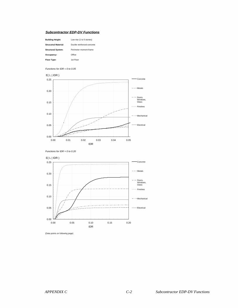
APPENDIX C C-2 Subcontractor EDP-DV Functions
Subcontractor EDP-DV Functions
Building Height: Low-rise (1 to 5 stories)
Strucutral Material: Ductile reinforced-concrete
Structural System: Perimeter moment-frame
Occupancy: Office
Floor Type: 1st Floor
Functions for IDR = 0 to 0.05
Functions for IDR = 0 to 0.20
(Data points on following page)
0.00
0.05
0.10
0.15
0.20
0.25
0.00 0.05 0.10 0.15 0.20
IDR
E( L | IDR )Concrete
Metals
Doors,Windows,Glass
Finishes
Mechanical
Electrical
0.00
0.05
0.10
0.15
0.20
0.25
0.00 0.01 0.02 0.03 0.04 0.05
IDR
E( L | IDR )Concrete
Metals
Doors,Windows,Glass
Finishes
Mechanical
Electrical

APPENDIX C C-3 Subcontractor EDP-DV Functions
Concrete Masonry Metals CarpentryMoisture
Protection
Doors, Windows,
GlassFinishes
Mech-anical
Electrical Concrete Masonry Metals CarpentryMoisture
Protection
Doors, Windows,
GlassFinishes
Mech-anical
Electrical
0.001 0.000 0.000 0.000 0.000 0.000 0.000 0.001 0.000 0.000 0.101 0.167 0.000 0.050 0.000 0.000 0.133 0.242 0.060 0.0860.002 0.000 0.000 0.001 0.000 0.000 0.002 0.006 0.000 0.000 0.102 0.167 0.000 0.050 0.000 0.000 0.133 0.242 0.060 0.086
0.003 0.000 0.000 0.002 0.000 0.000 0.003 0.011 0.001 0.000 0.103 0.168 0.000 0.050 0.000 0.000 0.133 0.242 0.060 0.086
0.004 0.001 0.000 0.003 0.000 0.000 0.004 0.018 0.001 0.000 0.104 0.169 0.000 0.050 0.000 0.000 0.133 0.242 0.060 0.086
0.005 0.002 0.000 0.004 0.000 0.000 0.007 0.029 0.001 0.002 0.105 0.170 0.000 0.050 0.000 0.000 0.133 0.242 0.060 0.086
0.006 0.003 0.000 0.006 0.000 0.000 0.010 0.045 0.002 0.004 0.106 0.171 0.000 0.050 0.000 0.000 0.133 0.242 0.060 0.086
0.007 0.006 0.000 0.008 0.000 0.000 0.014 0.062 0.003 0.008 0.107 0.171 0.000 0.050 0.000 0.000 0.133 0.242 0.060 0.086
0.008 0.008 0.000 0.010 0.000 0.000 0.017 0.080 0.004 0.013 0.108 0.172 0.000 0.050 0.000 0.000 0.133 0.242 0.060 0.086
0.009 0.011 0.000 0.012 0.000 0.000 0.020 0.098 0.005 0.019 0.109 0.173 0.000 0.050 0.000 0.000 0.133 0.242 0.060 0.086
0.010 0.014 0.000 0.014 0.000 0.000 0.023 0.115 0.007 0.026 0.110 0.173 0.000 0.050 0.000 0.000 0.133 0.242 0.060 0.086
0.011 0.017 0.000 0.016 0.000 0.000 0.026 0.130 0.009 0.032 0.111 0.174 0.000 0.050 0.000 0.000 0.133 0.242 0.061 0.0860.012 0.019 0.000 0.017 0.000 0.000 0.029 0.145 0.010 0.039 0.112 0.174 0.000 0.050 0.000 0.000 0.133 0.242 0.061 0.0860.013 0.021 0.000 0.019 0.000 0.000 0.031 0.158 0.012 0.045 0.113 0.175 0.000 0.050 0.000 0.000 0.133 0.242 0.061 0.0860.014 0.023 0.000 0.020 0.000 0.000 0.034 0.169 0.014 0.050 0.114 0.176 0.000 0.050 0.000 0.000 0.133 0.242 0.061 0.086
0.015 0.024 0.000 0.022 0.000 0.000 0.036 0.179 0.016 0.055 0.115 0.176 0.000 0.050 0.000 0.000 0.133 0.242 0.061 0.086
0.016 0.026 0.000 0.023 0.000 0.000 0.038 0.188 0.017 0.060 0.116 0.176 0.000 0.050 0.000 0.000 0.133 0.242 0.061 0.0860.017 0.027 0.000 0.024 0.000 0.000 0.040 0.195 0.019 0.064 0.117 0.177 0.000 0.050 0.000 0.000 0.133 0.242 0.061 0.0860.018 0.027 0.000 0.025 0.000 0.000 0.042 0.202 0.020 0.067 0.118 0.177 0.000 0.050 0.000 0.000 0.133 0.242 0.061 0.0860.019 0.028 0.000 0.026 0.000 0.000 0.044 0.207 0.021 0.070 0.119 0.178 0.000 0.050 0.000 0.000 0.133 0.242 0.061 0.0860.020 0.029 0.000 0.027 0.000 0.000 0.046 0.212 0.023 0.073 0.120 0.178 0.000 0.050 0.000 0.000 0.133 0.242 0.061 0.0860.021 0.029 0.000 0.028 0.000 0.000 0.048 0.216 0.024 0.075 0.121 0.179 0.000 0.050 0.000 0.000 0.133 0.242 0.061 0.0860.022 0.030 0.000 0.028 0.000 0.000 0.050 0.219 0.025 0.077 0.122 0.179 0.000 0.050 0.000 0.000 0.133 0.242 0.061 0.0860.023 0.030 0.000 0.029 0.000 0.000 0.053 0.222 0.026 0.078 0.123 0.179 0.000 0.051 0.000 0.000 0.133 0.242 0.061 0.0860.024 0.031 0.000 0.030 0.000 0.000 0.055 0.225 0.027 0.079 0.124 0.180 0.000 0.051 0.000 0.000 0.133 0.242 0.061 0.0860.025 0.031 0.000 0.031 0.000 0.000 0.058 0.227 0.029 0.080 0.125 0.180 0.000 0.051 0.000 0.000 0.133 0.242 0.061 0.0860.026 0.032 0.000 0.031 0.000 0.000 0.061 0.229 0.030 0.081 0.126 0.180 0.000 0.051 0.000 0.000 0.133 0.242 0.061 0.0860.027 0.032 0.000 0.032 0.000 0.000 0.064 0.230 0.031 0.082 0.127 0.180 0.000 0.051 0.000 0.000 0.133 0.242 0.061 0.0860.028 0.032 0.000 0.033 0.000 0.000 0.068 0.231 0.032 0.083 0.128 0.181 0.000 0.051 0.000 0.000 0.133 0.242 0.061 0.0860.029 0.033 0.000 0.033 0.000 0.000 0.071 0.232 0.033 0.083 0.129 0.181 0.000 0.051 0.000 0.000 0.133 0.242 0.062 0.0860.030 0.033 0.000 0.034 0.000 0.000 0.075 0.233 0.033 0.084 0.130 0.181 0.000 0.051 0.000 0.000 0.133 0.242 0.062 0.0860.031 0.034 0.000 0.034 0.000 0.000 0.078 0.234 0.034 0.084 0.131 0.181 0.000 0.051 0.000 0.000 0.133 0.242 0.062 0.0860.032 0.034 0.000 0.035 0.000 0.000 0.082 0.235 0.035 0.084 0.132 0.182 0.000 0.051 0.000 0.000 0.133 0.242 0.062 0.0860.033 0.035 0.000 0.035 0.000 0.000 0.086 0.235 0.036 0.085 0.133 0.182 0.000 0.051 0.000 0.000 0.133 0.242 0.062 0.0860.034 0.036 0.000 0.036 0.000 0.000 0.089 0.236 0.037 0.085 0.134 0.182 0.000 0.051 0.000 0.000 0.133 0.242 0.062 0.0860.035 0.036 0.000 0.036 0.000 0.000 0.093 0.236 0.038 0.085 0.135 0.182 0.000 0.051 0.000 0.000 0.133 0.242 0.062 0.0860.036 0.037 0.000 0.037 0.000 0.000 0.096 0.237 0.039 0.085 0.136 0.182 0.000 0.051 0.000 0.000 0.133 0.242 0.062 0.0860.037 0.038 0.000 0.037 0.000 0.000 0.099 0.237 0.039 0.085 0.137 0.182 0.000 0.051 0.000 0.000 0.133 0.242 0.062 0.0860.038 0.039 0.000 0.038 0.000 0.000 0.102 0.238 0.040 0.085 0.138 0.182 0.000 0.051 0.000 0.000 0.133 0.242 0.062 0.0860.039 0.040 0.000 0.038 0.000 0.000 0.105 0.238 0.041 0.086 0.139 0.183 0.000 0.051 0.000 0.000 0.133 0.242 0.062 0.0860.040 0.041 0.000 0.039 0.000 0.000 0.107 0.238 0.041 0.086 0.140 0.183 0.000 0.051 0.000 0.000 0.133 0.242 0.062 0.0860.041 0.042 0.000 0.039 0.000 0.000 0.110 0.238 0.042 0.086 0.141 0.183 0.000 0.051 0.000 0.000 0.133 0.242 0.062 0.0860.042 0.043 0.000 0.039 0.000 0.000 0.112 0.238 0.043 0.086 0.142 0.183 0.000 0.051 0.000 0.000 0.133 0.242 0.062 0.0860.043 0.045 0.000 0.040 0.000 0.000 0.114 0.239 0.043 0.086 0.143 0.183 0.000 0.051 0.000 0.000 0.133 0.242 0.062 0.0860.044 0.046 0.000 0.040 0.000 0.000 0.116 0.239 0.044 0.086 0.144 0.183 0.000 0.051 0.000 0.000 0.133 0.242 0.062 0.0860.045 0.048 0.000 0.041 0.000 0.000 0.118 0.239 0.045 0.086 0.145 0.183 0.000 0.051 0.000 0.000 0.133 0.242 0.062 0.0860.046 0.050 0.000 0.041 0.000 0.000 0.119 0.239 0.045 0.086 0.146 0.183 0.000 0.051 0.000 0.000 0.133 0.242 0.062 0.0860.047 0.052 0.000 0.041 0.000 0.000 0.121 0.239 0.046 0.086 0.147 0.183 0.000 0.051 0.000 0.000 0.133 0.242 0.062 0.0860.048 0.054 0.000 0.042 0.000 0.000 0.122 0.239 0.046 0.086 0.148 0.184 0.000 0.051 0.000 0.000 0.133 0.242 0.062 0.0860.049 0.057 0.000 0.042 0.000 0.000 0.123 0.240 0.047 0.086 0.149 0.184 0.000 0.051 0.000 0.000 0.133 0.242 0.062 0.0860.050 0.059 0.000 0.042 0.000 0.000 0.124 0.240 0.047 0.086 0.150 0.184 0.000 0.051 0.000 0.000 0.133 0.242 0.062 0.0860.051 0.062 0.000 0.042 0.000 0.000 0.125 0.240 0.048 0.086 0.151 0.184 0.000 0.051 0.000 0.000 0.133 0.242 0.062 0.0860.052 0.064 0.000 0.043 0.000 0.000 0.126 0.240 0.048 0.086 0.152 0.184 0.000 0.051 0.000 0.000 0.133 0.242 0.062 0.0860.053 0.067 0.000 0.043 0.000 0.000 0.127 0.240 0.049 0.086 0.153 0.184 0.000 0.051 0.000 0.000 0.133 0.242 0.062 0.086
0.054 0.070 0.000 0.043 0.000 0.000 0.128 0.240 0.049 0.086 0.154 0.184 0.000 0.051 0.000 0.000 0.133 0.242 0.062 0.086
0.055 0.073 0.000 0.044 0.000 0.000 0.128 0.240 0.050 0.086 0.155 0.184 0.000 0.051 0.000 0.000 0.133 0.242 0.062 0.0860.056 0.076 0.000 0.044 0.000 0.000 0.129 0.240 0.050 0.086 0.156 0.184 0.000 0.051 0.000 0.000 0.133 0.242 0.062 0.0860.057 0.079 0.000 0.044 0.000 0.000 0.129 0.240 0.050 0.086 0.157 0.184 0.000 0.051 0.000 0.000 0.133 0.242 0.062 0.0860.058 0.082 0.000 0.044 0.000 0.000 0.130 0.240 0.051 0.086 0.158 0.184 0.000 0.051 0.000 0.000 0.133 0.242 0.062 0.0860.059 0.085 0.000 0.044 0.000 0.000 0.130 0.240 0.051 0.086 0.159 0.184 0.000 0.051 0.000 0.000 0.133 0.242 0.062 0.0860.060 0.088 0.000 0.045 0.000 0.000 0.130 0.240 0.052 0.086 0.160 0.184 0.000 0.051 0.000 0.000 0.133 0.242 0.062 0.0860.061 0.091 0.000 0.045 0.000 0.000 0.131 0.240 0.052 0.086 0.161 0.184 0.000 0.051 0.000 0.000 0.133 0.242 0.062 0.0860.062 0.094 0.000 0.045 0.000 0.000 0.131 0.241 0.052 0.086 0.162 0.184 0.000 0.051 0.000 0.000 0.133 0.242 0.062 0.0860.063 0.097 0.000 0.045 0.000 0.000 0.131 0.241 0.053 0.086 0.163 0.184 0.000 0.051 0.000 0.000 0.133 0.242 0.062 0.0860.064 0.100 0.000 0.046 0.000 0.000 0.131 0.241 0.053 0.086 0.164 0.184 0.000 0.051 0.000 0.000 0.133 0.242 0.062 0.0860.065 0.103 0.000 0.046 0.000 0.000 0.131 0.241 0.053 0.086 0.165 0.184 0.000 0.051 0.000 0.000 0.133 0.242 0.062 0.0860.066 0.106 0.000 0.046 0.000 0.000 0.132 0.241 0.054 0.086 0.166 0.184 0.000 0.051 0.000 0.000 0.133 0.242 0.062 0.0860.067 0.109 0.000 0.046 0.000 0.000 0.132 0.241 0.054 0.086 0.167 0.184 0.000 0.051 0.000 0.000 0.133 0.242 0.062 0.0860.068 0.112 0.000 0.046 0.000 0.000 0.132 0.241 0.054 0.086 0.168 0.184 0.000 0.051 0.000 0.000 0.133 0.242 0.063 0.0860.069 0.114 0.000 0.046 0.000 0.000 0.132 0.241 0.054 0.086 0.169 0.184 0.000 0.051 0.000 0.000 0.133 0.242 0.063 0.0860.070 0.117 0.000 0.047 0.000 0.000 0.132 0.241 0.055 0.086 0.170 0.184 0.000 0.051 0.000 0.000 0.133 0.242 0.063 0.0860.071 0.119 0.000 0.047 0.000 0.000 0.132 0.241 0.055 0.086 0.171 0.184 0.000 0.051 0.000 0.000 0.133 0.242 0.063 0.0860.072 0.122 0.000 0.047 0.000 0.000 0.132 0.241 0.055 0.086 0.172 0.184 0.000 0.051 0.000 0.000 0.133 0.242 0.063 0.0860.073 0.124 0.000 0.047 0.000 0.000 0.132 0.241 0.055 0.086 0.173 0.184 0.000 0.051 0.000 0.000 0.133 0.242 0.063 0.0860.074 0.126 0.000 0.047 0.000 0.000 0.132 0.241 0.056 0.086 0.174 0.184 0.000 0.051 0.000 0.000 0.133 0.242 0.063 0.0860.075 0.129 0.000 0.047 0.000 0.000 0.132 0.241 0.056 0.086 0.175 0.184 0.000 0.051 0.000 0.000 0.133 0.242 0.063 0.0860.076 0.131 0.000 0.047 0.000 0.000 0.133 0.241 0.056 0.086 0.176 0.184 0.000 0.051 0.000 0.000 0.133 0.242 0.063 0.0860.077 0.133 0.000 0.048 0.000 0.000 0.133 0.241 0.056 0.086 0.177 0.184 0.000 0.051 0.000 0.000 0.133 0.242 0.063 0.0860.078 0.135 0.000 0.048 0.000 0.000 0.133 0.241 0.056 0.086 0.178 0.184 0.000 0.051 0.000 0.000 0.133 0.242 0.063 0.0860.079 0.137 0.000 0.048 0.000 0.000 0.133 0.241 0.057 0.086 0.179 0.184 0.000 0.051 0.000 0.000 0.133 0.242 0.063 0.0860.080 0.139 0.000 0.048 0.000 0.000 0.133 0.241 0.057 0.086 0.180 0.184 0.000 0.051 0.000 0.000 0.133 0.242 0.063 0.0860.081 0.140 0.000 0.048 0.000 0.000 0.133 0.241 0.057 0.086 0.181 0.184 0.000 0.051 0.000 0.000 0.133 0.242 0.063 0.0860.082 0.142 0.000 0.048 0.000 0.000 0.133 0.241 0.057 0.086 0.182 0.184 0.000 0.051 0.000 0.000 0.133 0.242 0.063 0.0860.083 0.144 0.000 0.048 0.000 0.000 0.133 0.241 0.057 0.086 0.183 0.184 0.000 0.051 0.000 0.000 0.133 0.242 0.063 0.0860.084 0.146 0.000 0.048 0.000 0.000 0.133 0.241 0.058 0.086 0.184 0.184 0.000 0.051 0.000 0.000 0.133 0.242 0.063 0.0860.085 0.147 0.000 0.048 0.000 0.000 0.133 0.241 0.058 0.086 0.185 0.184 0.000 0.051 0.000 0.000 0.133 0.242 0.063 0.0860.086 0.149 0.000 0.048 0.000 0.000 0.133 0.241 0.058 0.086 0.186 0.184 0.000 0.051 0.000 0.000 0.133 0.242 0.063 0.0860.087 0.150 0.000 0.049 0.000 0.000 0.133 0.241 0.058 0.086 0.187 0.185 0.000 0.051 0.000 0.000 0.133 0.242 0.063 0.0860.088 0.152 0.000 0.049 0.000 0.000 0.133 0.241 0.058 0.086 0.188 0.185 0.000 0.051 0.000 0.000 0.134 0.242 0.063 0.0860.089 0.153 0.000 0.049 0.000 0.000 0.133 0.241 0.058 0.086 0.189 0.185 0.000 0.051 0.000 0.000 0.134 0.242 0.063 0.0860.090 0.154 0.000 0.049 0.000 0.000 0.133 0.242 0.058 0.086 0.190 0.185 0.000 0.051 0.000 0.000 0.134 0.242 0.063 0.0860.091 0.156 0.000 0.049 0.000 0.000 0.133 0.242 0.059 0.086 0.191 0.185 0.000 0.051 0.000 0.000 0.134 0.242 0.063 0.0860.092 0.157 0.000 0.049 0.000 0.000 0.133 0.242 0.059 0.086 0.192 0.185 0.000 0.051 0.000 0.000 0.134 0.242 0.063 0.0860.093 0.158 0.000 0.049 0.000 0.000 0.133 0.242 0.059 0.086 0.193 0.185 0.000 0.051 0.000 0.000 0.134 0.242 0.063 0.0860.094 0.159 0.000 0.049 0.000 0.000 0.133 0.242 0.059 0.086 0.194 0.185 0.000 0.051 0.000 0.000 0.134 0.242 0.063 0.0860.095 0.160 0.000 0.049 0.000 0.000 0.133 0.242 0.059 0.086 0.195 0.185 0.000 0.051 0.000 0.000 0.134 0.242 0.063 0.0860.096 0.162 0.000 0.049 0.000 0.000 0.133 0.242 0.059 0.086 0.196 0.185 0.000 0.051 0.000 0.000 0.134 0.242 0.063 0.0860.097 0.163 0.000 0.049 0.000 0.000 0.133 0.242 0.059 0.086 0.197 0.185 0.000 0.051 0.000 0.000 0.134 0.242 0.063 0.0860.098 0.164 0.000 0.049 0.000 0.000 0.133 0.242 0.059 0.086 0.198 0.185 0.000 0.051 0.000 0.000 0.134 0.242 0.063 0.0860.099 0.165 0.000 0.049 0.000 0.000 0.133 0.242 0.060 0.086 0.199 0.185 0.000 0.051 0.000 0.000 0.134 0.242 0.063 0.0860.100 0.166 0.000 0.050 0.000 0.000 0.133 0.242 0.060 0.086 0.200 0.185 0.000 0.051 0.000 0.000 0.134 0.242 0.063 0.086
EDP-DV Function
IDR IDR
EDP-DV Function (cont'd)

APPENDIX C C-4 Subcontractor EDP-DV Functions
Subcontractor EDP-DV Functions
Building Height: Low-rise (1 to 5 stories)
Strucutral Material: Ductile reinforced-concrete
Structural System: Perimeter moment-frame
Occupancy: Office
Floor Type: Typical Floor
Functions for IDR = 0 to 0.05
Functions for IDR = 0 to 0.20
(Data points on following page)
0.00
0.05
0.10
0.15
0.20
0.25
0.00 0.05 0.10 0.15 0.20
IDR
E( L | IDR )Concrete
Metals
Doors,Windows,Glass
Finishes
Mechanical
Electrical
0.00
0.05
0.10
0.15
0.20
0.25
0.00 0.01 0.02 0.03 0.04 0.05
IDR
E( L | IDR )Concrete
Metals
Doors,Windows,Glass
Finishes
Mechanical
Electrical
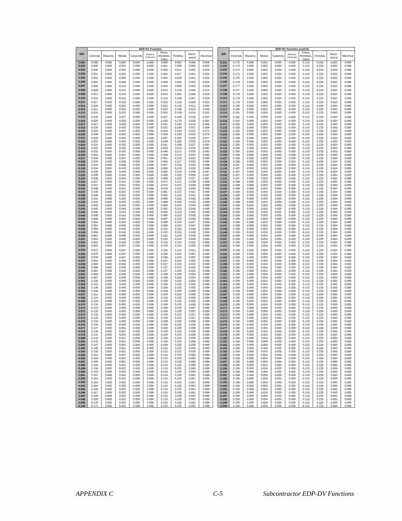
APPENDIX C C-5 Subcontractor EDP-DV Functions
Concrete Masonry Metals CarpentryMoisture
Protection
Doors, Windows,
GlassFinishes
Mech-anical
Electrical Concrete Masonry Metals CarpentryMoisture
Protection
Doors, Windows,
GlassFinishes
Mech-anical
Electrical
0.001 0.000 0.000 0.000 0.000 0.000 0.000 0.001 0.000 0.000 0.101 0.172 0.000 0.052 0.000 0.000 0.110 0.226 0.062 0.0890.002 0.000 0.000 0.001 0.000 0.000 0.001 0.006 0.000 0.000 0.102 0.173 0.000 0.052 0.000 0.000 0.110 0.226 0.062 0.089
0.003 0.000 0.000 0.002 0.000 0.000 0.002 0.011 0.001 0.000 0.103 0.174 0.000 0.052 0.000 0.000 0.110 0.226 0.062 0.089
0.004 0.001 0.000 0.003 0.000 0.000 0.003 0.017 0.001 0.000 0.104 0.174 0.000 0.052 0.000 0.000 0.110 0.226 0.062 0.089
0.005 0.002 0.000 0.005 0.000 0.000 0.005 0.028 0.001 0.002 0.105 0.175 0.000 0.052 0.000 0.000 0.110 0.226 0.062 0.089
0.006 0.003 0.000 0.008 0.000 0.000 0.008 0.042 0.002 0.004 0.106 0.176 0.000 0.052 0.000 0.000 0.110 0.226 0.062 0.089
0.007 0.006 0.000 0.010 0.000 0.000 0.010 0.059 0.003 0.008 0.107 0.177 0.000 0.053 0.000 0.000 0.110 0.226 0.062 0.089
0.008 0.009 0.000 0.013 0.000 0.000 0.013 0.076 0.004 0.014 0.108 0.177 0.000 0.053 0.000 0.000 0.110 0.226 0.062 0.089
0.009 0.012 0.000 0.015 0.000 0.000 0.015 0.092 0.005 0.020 0.109 0.178 0.000 0.053 0.000 0.000 0.110 0.226 0.062 0.089
0.010 0.015 0.000 0.018 0.000 0.000 0.018 0.108 0.007 0.026 0.110 0.179 0.000 0.053 0.000 0.000 0.110 0.226 0.062 0.089
0.011 0.017 0.000 0.020 0.000 0.000 0.020 0.123 0.009 0.033 0.111 0.179 0.000 0.053 0.000 0.000 0.110 0.226 0.063 0.0890.012 0.020 0.000 0.022 0.000 0.000 0.022 0.136 0.011 0.040 0.112 0.180 0.000 0.053 0.000 0.000 0.110 0.226 0.063 0.0890.013 0.022 0.000 0.024 0.000 0.000 0.024 0.148 0.013 0.046 0.113 0.180 0.000 0.053 0.000 0.000 0.110 0.226 0.063 0.0890.014 0.024 0.000 0.025 0.000 0.000 0.026 0.159 0.014 0.052 0.114 0.181 0.000 0.053 0.000 0.000 0.110 0.226 0.063 0.089
0.015 0.025 0.000 0.027 0.000 0.000 0.027 0.168 0.016 0.057 0.115 0.182 0.000 0.053 0.000 0.000 0.110 0.226 0.063 0.089
0.016 0.026 0.000 0.028 0.000 0.000 0.029 0.176 0.018 0.062 0.116 0.182 0.000 0.053 0.000 0.000 0.110 0.226 0.063 0.0890.017 0.027 0.000 0.029 0.000 0.000 0.031 0.183 0.019 0.066 0.117 0.183 0.000 0.053 0.000 0.000 0.110 0.226 0.063 0.0890.018 0.028 0.000 0.030 0.000 0.000 0.032 0.189 0.021 0.069 0.118 0.183 0.000 0.053 0.000 0.000 0.110 0.226 0.063 0.0890.019 0.029 0.000 0.031 0.000 0.000 0.034 0.194 0.022 0.072 0.119 0.183 0.000 0.053 0.000 0.000 0.110 0.226 0.063 0.0890.020 0.030 0.000 0.032 0.000 0.000 0.036 0.199 0.023 0.075 0.120 0.184 0.000 0.053 0.000 0.000 0.110 0.226 0.063 0.0890.021 0.030 0.000 0.033 0.000 0.000 0.037 0.202 0.025 0.077 0.121 0.184 0.000 0.053 0.000 0.000 0.110 0.226 0.063 0.0890.022 0.031 0.000 0.034 0.000 0.000 0.039 0.205 0.026 0.079 0.122 0.185 0.000 0.053 0.000 0.000 0.110 0.226 0.063 0.0890.023 0.031 0.000 0.035 0.000 0.000 0.041 0.208 0.027 0.081 0.123 0.185 0.000 0.053 0.000 0.000 0.110 0.226 0.063 0.0890.024 0.032 0.000 0.035 0.000 0.000 0.043 0.210 0.028 0.082 0.124 0.185 0.000 0.053 0.000 0.000 0.110 0.226 0.063 0.0890.025 0.032 0.000 0.036 0.000 0.000 0.046 0.212 0.029 0.083 0.125 0.185 0.000 0.053 0.000 0.000 0.110 0.226 0.063 0.0890.026 0.032 0.000 0.037 0.000 0.000 0.048 0.214 0.031 0.084 0.126 0.186 0.000 0.053 0.000 0.000 0.110 0.226 0.063 0.0890.027 0.033 0.000 0.037 0.000 0.000 0.051 0.215 0.032 0.085 0.127 0.186 0.000 0.053 0.000 0.000 0.110 0.226 0.063 0.0890.028 0.033 0.000 0.038 0.000 0.000 0.054 0.217 0.033 0.085 0.128 0.186 0.000 0.053 0.000 0.000 0.110 0.226 0.064 0.0890.029 0.034 0.000 0.038 0.000 0.000 0.057 0.218 0.034 0.086 0.129 0.187 0.000 0.053 0.000 0.000 0.110 0.226 0.064 0.0890.030 0.034 0.000 0.039 0.000 0.000 0.060 0.218 0.035 0.086 0.130 0.187 0.000 0.053 0.000 0.000 0.110 0.226 0.064 0.0890.031 0.035 0.000 0.039 0.000 0.000 0.063 0.219 0.036 0.087 0.131 0.187 0.000 0.053 0.000 0.000 0.110 0.226 0.064 0.0890.032 0.035 0.000 0.040 0.000 0.000 0.066 0.220 0.036 0.087 0.132 0.187 0.000 0.053 0.000 0.000 0.110 0.226 0.064 0.0890.033 0.036 0.000 0.040 0.000 0.000 0.069 0.220 0.037 0.087 0.133 0.187 0.000 0.053 0.000 0.000 0.110 0.226 0.064 0.0890.034 0.037 0.000 0.041 0.000 0.000 0.072 0.221 0.038 0.088 0.134 0.188 0.000 0.053 0.000 0.000 0.110 0.226 0.064 0.0890.035 0.037 0.000 0.041 0.000 0.000 0.075 0.221 0.039 0.088 0.135 0.188 0.000 0.053 0.000 0.000 0.110 0.226 0.064 0.0890.036 0.038 0.000 0.041 0.000 0.000 0.078 0.222 0.040 0.088 0.136 0.188 0.000 0.053 0.000 0.000 0.110 0.226 0.064 0.0890.037 0.039 0.000 0.042 0.000 0.000 0.081 0.222 0.041 0.088 0.137 0.188 0.000 0.053 0.000 0.000 0.110 0.226 0.064 0.0890.038 0.040 0.000 0.042 0.000 0.000 0.083 0.222 0.041 0.088 0.138 0.188 0.000 0.053 0.000 0.000 0.110 0.226 0.064 0.0890.039 0.041 0.000 0.043 0.000 0.000 0.086 0.222 0.042 0.088 0.139 0.188 0.000 0.053 0.000 0.000 0.110 0.226 0.064 0.0890.040 0.042 0.000 0.043 0.000 0.000 0.088 0.223 0.043 0.088 0.140 0.189 0.000 0.053 0.000 0.000 0.110 0.226 0.064 0.0890.041 0.043 0.000 0.043 0.000 0.000 0.090 0.223 0.043 0.089 0.141 0.189 0.000 0.053 0.000 0.000 0.110 0.226 0.064 0.0890.042 0.045 0.000 0.044 0.000 0.000 0.092 0.223 0.044 0.089 0.142 0.189 0.000 0.053 0.000 0.000 0.110 0.226 0.064 0.0890.043 0.046 0.000 0.044 0.000 0.000 0.094 0.223 0.045 0.089 0.143 0.189 0.000 0.053 0.000 0.000 0.110 0.226 0.064 0.0890.044 0.048 0.000 0.044 0.000 0.000 0.095 0.223 0.045 0.089 0.144 0.189 0.000 0.053 0.000 0.000 0.110 0.226 0.064 0.0890.045 0.050 0.000 0.045 0.000 0.000 0.097 0.223 0.046 0.089 0.145 0.189 0.000 0.053 0.000 0.000 0.110 0.226 0.064 0.0890.046 0.052 0.000 0.045 0.000 0.000 0.098 0.224 0.047 0.089 0.146 0.189 0.000 0.053 0.000 0.000 0.110 0.226 0.064 0.0890.047 0.054 0.000 0.045 0.000 0.000 0.099 0.224 0.047 0.089 0.147 0.189 0.000 0.053 0.000 0.000 0.110 0.226 0.064 0.0890.048 0.056 0.000 0.045 0.000 0.000 0.101 0.224 0.048 0.089 0.148 0.189 0.000 0.053 0.000 0.000 0.110 0.226 0.064 0.0890.049 0.058 0.000 0.046 0.000 0.000 0.102 0.224 0.048 0.089 0.149 0.189 0.000 0.054 0.000 0.000 0.110 0.226 0.064 0.0890.050 0.061 0.000 0.046 0.000 0.000 0.102 0.224 0.049 0.089 0.150 0.189 0.000 0.054 0.000 0.000 0.110 0.226 0.064 0.0890.051 0.064 0.000 0.046 0.000 0.000 0.103 0.224 0.049 0.089 0.151 0.189 0.000 0.054 0.000 0.000 0.110 0.226 0.064 0.0890.052 0.066 0.000 0.046 0.000 0.000 0.104 0.224 0.050 0.089 0.152 0.190 0.000 0.054 0.000 0.000 0.110 0.226 0.064 0.0890.053 0.069 0.000 0.047 0.000 0.000 0.105 0.224 0.050 0.089 0.153 0.190 0.000 0.054 0.000 0.000 0.110 0.226 0.064 0.089
0.054 0.072 0.000 0.047 0.000 0.000 0.105 0.224 0.051 0.089 0.154 0.190 0.000 0.054 0.000 0.000 0.110 0.226 0.064 0.089
0.055 0.075 0.000 0.047 0.000 0.000 0.106 0.224 0.051 0.089 0.155 0.190 0.000 0.054 0.000 0.000 0.110 0.226 0.064 0.0890.056 0.078 0.000 0.047 0.000 0.000 0.106 0.224 0.052 0.089 0.156 0.190 0.000 0.054 0.000 0.000 0.110 0.226 0.064 0.0890.057 0.082 0.000 0.048 0.000 0.000 0.107 0.224 0.052 0.089 0.157 0.190 0.000 0.054 0.000 0.000 0.110 0.226 0.064 0.0890.058 0.085 0.000 0.048 0.000 0.000 0.107 0.224 0.052 0.089 0.158 0.190 0.000 0.054 0.000 0.000 0.110 0.226 0.064 0.0890.059 0.088 0.000 0.048 0.000 0.000 0.107 0.224 0.053 0.089 0.159 0.190 0.000 0.054 0.000 0.000 0.110 0.226 0.064 0.0890.060 0.091 0.000 0.048 0.000 0.000 0.107 0.225 0.053 0.089 0.160 0.190 0.000 0.054 0.000 0.000 0.110 0.226 0.064 0.0890.061 0.094 0.000 0.048 0.000 0.000 0.108 0.225 0.054 0.089 0.161 0.190 0.000 0.054 0.000 0.000 0.110 0.226 0.064 0.0890.062 0.097 0.000 0.048 0.000 0.000 0.108 0.225 0.054 0.089 0.162 0.190 0.000 0.054 0.000 0.000 0.110 0.226 0.064 0.0890.063 0.100 0.000 0.049 0.000 0.000 0.108 0.225 0.054 0.089 0.163 0.190 0.000 0.054 0.000 0.000 0.110 0.226 0.065 0.0890.064 0.103 0.000 0.049 0.000 0.000 0.108 0.225 0.055 0.089 0.164 0.190 0.000 0.054 0.000 0.000 0.110 0.226 0.065 0.0890.065 0.106 0.000 0.049 0.000 0.000 0.108 0.225 0.055 0.089 0.165 0.190 0.000 0.054 0.000 0.000 0.110 0.226 0.065 0.0890.066 0.109 0.000 0.049 0.000 0.000 0.109 0.225 0.055 0.089 0.166 0.190 0.000 0.054 0.000 0.000 0.110 0.226 0.065 0.0890.067 0.112 0.000 0.049 0.000 0.000 0.109 0.225 0.056 0.089 0.167 0.190 0.000 0.054 0.000 0.000 0.110 0.226 0.065 0.0890.068 0.115 0.000 0.049 0.000 0.000 0.109 0.225 0.056 0.089 0.168 0.190 0.000 0.054 0.000 0.000 0.110 0.226 0.065 0.0890.069 0.118 0.000 0.050 0.000 0.000 0.109 0.225 0.056 0.089 0.169 0.190 0.000 0.054 0.000 0.000 0.110 0.226 0.065 0.0890.070 0.120 0.000 0.050 0.000 0.000 0.109 0.225 0.056 0.089 0.170 0.190 0.000 0.054 0.000 0.000 0.110 0.226 0.065 0.0890.071 0.123 0.000 0.050 0.000 0.000 0.109 0.225 0.057 0.089 0.171 0.190 0.000 0.054 0.000 0.000 0.110 0.226 0.065 0.0890.072 0.126 0.000 0.050 0.000 0.000 0.109 0.225 0.057 0.089 0.172 0.190 0.000 0.054 0.000 0.000 0.110 0.226 0.065 0.0890.073 0.128 0.000 0.050 0.000 0.000 0.109 0.225 0.057 0.089 0.173 0.190 0.000 0.054 0.000 0.000 0.110 0.226 0.065 0.0890.074 0.130 0.000 0.050 0.000 0.000 0.109 0.225 0.057 0.089 0.174 0.190 0.000 0.054 0.000 0.000 0.110 0.226 0.065 0.0890.075 0.133 0.000 0.050 0.000 0.000 0.109 0.225 0.058 0.089 0.175 0.190 0.000 0.054 0.000 0.000 0.110 0.226 0.065 0.0890.076 0.135 0.000 0.050 0.000 0.000 0.109 0.225 0.058 0.089 0.176 0.190 0.000 0.054 0.000 0.000 0.110 0.226 0.065 0.0890.077 0.137 0.000 0.051 0.000 0.000 0.109 0.225 0.058 0.089 0.177 0.190 0.000 0.054 0.000 0.000 0.110 0.226 0.065 0.0890.078 0.139 0.000 0.051 0.000 0.000 0.109 0.225 0.058 0.089 0.178 0.190 0.000 0.054 0.000 0.000 0.110 0.226 0.065 0.0890.079 0.141 0.000 0.051 0.000 0.000 0.109 0.225 0.059 0.089 0.179 0.190 0.000 0.054 0.000 0.000 0.110 0.226 0.065 0.0890.080 0.143 0.000 0.051 0.000 0.000 0.109 0.225 0.059 0.089 0.180 0.190 0.000 0.054 0.000 0.000 0.110 0.226 0.065 0.0890.081 0.145 0.000 0.051 0.000 0.000 0.109 0.225 0.059 0.089 0.181 0.190 0.000 0.054 0.000 0.000 0.110 0.226 0.065 0.0890.082 0.147 0.000 0.051 0.000 0.000 0.109 0.225 0.059 0.089 0.182 0.190 0.000 0.054 0.000 0.000 0.110 0.226 0.065 0.0890.083 0.148 0.000 0.051 0.000 0.000 0.110 0.225 0.059 0.089 0.183 0.190 0.000 0.054 0.000 0.000 0.110 0.226 0.065 0.0890.084 0.150 0.000 0.051 0.000 0.000 0.110 0.225 0.059 0.089 0.184 0.190 0.000 0.054 0.000 0.000 0.110 0.226 0.065 0.0890.085 0.152 0.000 0.051 0.000 0.000 0.110 0.225 0.060 0.089 0.185 0.190 0.000 0.054 0.000 0.000 0.110 0.226 0.065 0.0890.086 0.153 0.000 0.051 0.000 0.000 0.110 0.225 0.060 0.089 0.186 0.190 0.000 0.054 0.000 0.000 0.110 0.226 0.065 0.0890.087 0.155 0.000 0.051 0.000 0.000 0.110 0.225 0.060 0.089 0.187 0.190 0.000 0.054 0.000 0.000 0.110 0.226 0.065 0.0890.088 0.156 0.000 0.051 0.000 0.000 0.110 0.225 0.060 0.089 0.188 0.190 0.000 0.054 0.000 0.000 0.110 0.226 0.065 0.0890.089 0.158 0.000 0.052 0.000 0.000 0.110 0.225 0.060 0.089 0.189 0.190 0.000 0.054 0.000 0.000 0.110 0.226 0.065 0.0890.090 0.159 0.000 0.052 0.000 0.000 0.110 0.225 0.060 0.089 0.190 0.190 0.000 0.054 0.000 0.000 0.110 0.226 0.065 0.0890.091 0.161 0.000 0.052 0.000 0.000 0.110 0.225 0.061 0.089 0.191 0.190 0.000 0.054 0.000 0.000 0.110 0.226 0.065 0.0890.092 0.162 0.000 0.052 0.000 0.000 0.110 0.225 0.061 0.089 0.192 0.190 0.000 0.054 0.000 0.000 0.110 0.226 0.065 0.0890.093 0.163 0.000 0.052 0.000 0.000 0.110 0.225 0.061 0.089 0.193 0.190 0.000 0.054 0.000 0.000 0.110 0.226 0.065 0.0890.094 0.164 0.000 0.052 0.000 0.000 0.110 0.225 0.061 0.089 0.194 0.190 0.000 0.054 0.000 0.000 0.110 0.226 0.065 0.0890.095 0.166 0.000 0.052 0.000 0.000 0.110 0.225 0.061 0.089 0.195 0.190 0.000 0.054 0.000 0.000 0.110 0.226 0.065 0.0890.096 0.167 0.000 0.052 0.000 0.000 0.110 0.226 0.061 0.089 0.196 0.190 0.000 0.054 0.000 0.000 0.110 0.226 0.065 0.0890.097 0.168 0.000 0.052 0.000 0.000 0.110 0.226 0.061 0.089 0.197 0.190 0.000 0.054 0.000 0.000 0.110 0.226 0.065 0.0890.098 0.169 0.000 0.052 0.000 0.000 0.110 0.226 0.061 0.089 0.198 0.190 0.000 0.054 0.000 0.000 0.110 0.226 0.065 0.0890.099 0.170 0.000 0.052 0.000 0.000 0.110 0.226 0.061 0.089 0.199 0.190 0.000 0.054 0.000 0.000 0.110 0.226 0.065 0.0890.100 0.171 0.000 0.052 0.000 0.000 0.110 0.226 0.062 0.089 0.200 0.190 0.000 0.054 0.000 0.000 0.110 0.226 0.065 0.089
EDP-DV Function
IDR IDR
EDP-DV Function (cont'd)

APPENDIX C C-6 Subcontractor EDP-DV Functions
Subcontractor EDP-DV Functions
Building Height: Low-rise (1 to 5 stories)
Strucutral Material: Ductile reinforced-concrete
Structural System: Perimeter moment-frame
Occupancy: Office
Floor Type: Top Floor
Functions for IDR = 0 to 0.05
Functions for IDR = 0 to 0.20
(Data points on following page)
0.00
0.05
0.10
0.15
0.20
0.25
0.00 0.05 0.10 0.15 0.20
IDR
E( L | IDR )Concrete
Metals
Doors,Windows,Glass
Finishes
Mechanical
Electrical
0.00
0.05
0.10
0.15
0.20
0.25
0.00 0.01 0.02 0.03 0.04 0.05
IDR
E( L | IDR )Concrete
Metals
Doors,Windows,Glass
Finishes
Mechanical
Electrical

APPENDIX C C-7 Subcontractor EDP-DV Functions
Concrete Masonry Metals CarpentryMoisture
Protection
Doors, Windows,
GlassFinishes
Mech-anical
Electrical Concrete Masonry Metals CarpentryMoisture
Protection
Doors, Windows,
GlassFinishes
Mech-anical
Electrical
0.001 0.000 0.000 0.000 0.000 0.000 0.000 0.001 0.000 0.000 0.101 0.141 0.000 0.026 0.000 0.000 0.094 0.174 0.079 0.0910.002 0.000 0.000 0.000 0.000 0.000 0.001 0.005 0.000 0.000 0.102 0.142 0.000 0.026 0.000 0.000 0.094 0.174 0.079 0.091
0.003 0.000 0.000 0.001 0.000 0.000 0.001 0.009 0.001 0.000 0.103 0.142 0.000 0.026 0.000 0.000 0.094 0.174 0.079 0.091
0.004 0.001 0.000 0.001 0.000 0.000 0.002 0.015 0.001 0.000 0.104 0.143 0.000 0.026 0.000 0.000 0.094 0.174 0.079 0.091
0.005 0.001 0.000 0.002 0.000 0.000 0.002 0.024 0.002 0.002 0.105 0.144 0.000 0.026 0.000 0.000 0.095 0.174 0.079 0.091
0.006 0.003 0.000 0.003 0.000 0.000 0.004 0.035 0.002 0.004 0.106 0.144 0.000 0.026 0.000 0.000 0.095 0.174 0.079 0.091
0.007 0.005 0.000 0.004 0.000 0.000 0.005 0.049 0.003 0.008 0.107 0.145 0.000 0.027 0.000 0.000 0.095 0.174 0.079 0.091
0.008 0.007 0.000 0.005 0.000 0.000 0.006 0.062 0.005 0.014 0.108 0.146 0.000 0.027 0.000 0.000 0.095 0.174 0.080 0.091
0.009 0.009 0.000 0.006 0.000 0.000 0.007 0.075 0.006 0.020 0.109 0.146 0.000 0.027 0.000 0.000 0.095 0.174 0.080 0.091
0.010 0.012 0.000 0.007 0.000 0.000 0.008 0.087 0.009 0.027 0.110 0.147 0.000 0.027 0.000 0.000 0.095 0.174 0.080 0.091
0.011 0.014 0.000 0.008 0.000 0.000 0.010 0.098 0.011 0.034 0.111 0.147 0.000 0.027 0.000 0.000 0.095 0.174 0.080 0.0910.012 0.016 0.000 0.009 0.000 0.000 0.011 0.109 0.013 0.041 0.112 0.148 0.000 0.027 0.000 0.000 0.095 0.174 0.080 0.0910.013 0.018 0.000 0.010 0.000 0.000 0.012 0.117 0.015 0.048 0.113 0.148 0.000 0.027 0.000 0.000 0.095 0.174 0.080 0.0910.014 0.020 0.000 0.011 0.000 0.000 0.013 0.125 0.017 0.054 0.114 0.149 0.000 0.027 0.000 0.000 0.095 0.174 0.080 0.091
0.015 0.021 0.000 0.011 0.000 0.000 0.014 0.132 0.019 0.059 0.115 0.149 0.000 0.027 0.000 0.000 0.095 0.174 0.080 0.091
0.016 0.022 0.000 0.012 0.000 0.000 0.016 0.138 0.021 0.064 0.116 0.149 0.000 0.027 0.000 0.000 0.095 0.174 0.080 0.0910.017 0.022 0.000 0.013 0.000 0.000 0.017 0.143 0.023 0.068 0.117 0.150 0.000 0.027 0.000 0.000 0.095 0.174 0.080 0.0910.018 0.023 0.000 0.013 0.000 0.000 0.018 0.148 0.025 0.071 0.118 0.150 0.000 0.027 0.000 0.000 0.095 0.174 0.080 0.0910.019 0.024 0.000 0.014 0.000 0.000 0.019 0.152 0.027 0.074 0.119 0.151 0.000 0.027 0.000 0.000 0.095 0.174 0.081 0.0910.020 0.024 0.000 0.014 0.000 0.000 0.021 0.155 0.028 0.077 0.120 0.151 0.000 0.027 0.000 0.000 0.095 0.174 0.081 0.0910.021 0.025 0.000 0.015 0.000 0.000 0.022 0.157 0.030 0.079 0.121 0.151 0.000 0.027 0.000 0.000 0.095 0.174 0.081 0.0910.022 0.025 0.000 0.015 0.000 0.000 0.024 0.160 0.032 0.081 0.122 0.151 0.000 0.027 0.000 0.000 0.095 0.174 0.081 0.0910.023 0.025 0.000 0.016 0.000 0.000 0.026 0.162 0.033 0.083 0.123 0.152 0.000 0.027 0.000 0.000 0.095 0.174 0.081 0.0910.024 0.026 0.000 0.016 0.000 0.000 0.028 0.163 0.035 0.084 0.124 0.152 0.000 0.027 0.000 0.000 0.095 0.174 0.081 0.0910.025 0.026 0.000 0.016 0.000 0.000 0.030 0.165 0.036 0.085 0.125 0.152 0.000 0.027 0.000 0.000 0.095 0.174 0.081 0.0910.026 0.027 0.000 0.017 0.000 0.000 0.033 0.166 0.037 0.086 0.126 0.153 0.000 0.027 0.000 0.000 0.095 0.174 0.081 0.0910.027 0.027 0.000 0.017 0.000 0.000 0.035 0.167 0.039 0.087 0.127 0.153 0.000 0.027 0.000 0.000 0.095 0.174 0.081 0.0910.028 0.027 0.000 0.017 0.000 0.000 0.038 0.168 0.040 0.088 0.128 0.153 0.000 0.027 0.000 0.000 0.095 0.174 0.081 0.0910.029 0.028 0.000 0.018 0.000 0.000 0.041 0.169 0.041 0.088 0.129 0.153 0.000 0.027 0.000 0.000 0.095 0.174 0.081 0.0910.030 0.028 0.000 0.018 0.000 0.000 0.044 0.169 0.043 0.089 0.130 0.153 0.000 0.027 0.000 0.000 0.095 0.174 0.081 0.0910.031 0.029 0.000 0.018 0.000 0.000 0.047 0.170 0.044 0.089 0.131 0.154 0.000 0.027 0.000 0.000 0.095 0.174 0.081 0.0910.032 0.029 0.000 0.019 0.000 0.000 0.050 0.170 0.045 0.090 0.132 0.154 0.000 0.027 0.000 0.000 0.095 0.174 0.081 0.0910.033 0.029 0.000 0.019 0.000 0.000 0.054 0.171 0.046 0.090 0.133 0.154 0.000 0.027 0.000 0.000 0.095 0.174 0.081 0.0910.034 0.030 0.000 0.019 0.000 0.000 0.057 0.171 0.047 0.090 0.134 0.154 0.000 0.027 0.000 0.000 0.095 0.174 0.082 0.0910.035 0.031 0.000 0.019 0.000 0.000 0.060 0.171 0.049 0.090 0.135 0.154 0.000 0.027 0.000 0.000 0.095 0.174 0.082 0.0910.036 0.031 0.000 0.020 0.000 0.000 0.062 0.171 0.050 0.091 0.136 0.154 0.000 0.027 0.000 0.000 0.095 0.174 0.082 0.0910.037 0.032 0.000 0.020 0.000 0.000 0.065 0.172 0.051 0.091 0.137 0.154 0.000 0.027 0.000 0.000 0.095 0.174 0.082 0.0910.038 0.033 0.000 0.020 0.000 0.000 0.068 0.172 0.052 0.091 0.138 0.155 0.000 0.027 0.000 0.000 0.095 0.174 0.082 0.0910.039 0.033 0.000 0.020 0.000 0.000 0.070 0.172 0.053 0.091 0.139 0.155 0.000 0.027 0.000 0.000 0.095 0.174 0.082 0.0910.040 0.034 0.000 0.021 0.000 0.000 0.073 0.172 0.054 0.091 0.140 0.155 0.000 0.027 0.000 0.000 0.095 0.174 0.082 0.0910.041 0.035 0.000 0.021 0.000 0.000 0.075 0.172 0.055 0.091 0.141 0.155 0.000 0.027 0.000 0.000 0.095 0.174 0.082 0.0910.042 0.036 0.000 0.021 0.000 0.000 0.077 0.172 0.055 0.091 0.142 0.155 0.000 0.027 0.000 0.000 0.095 0.174 0.082 0.0910.043 0.038 0.000 0.021 0.000 0.000 0.078 0.173 0.056 0.091 0.143 0.155 0.000 0.027 0.000 0.000 0.095 0.174 0.082 0.0910.044 0.039 0.000 0.021 0.000 0.000 0.080 0.173 0.057 0.091 0.144 0.155 0.000 0.027 0.000 0.000 0.095 0.174 0.082 0.0910.045 0.041 0.000 0.022 0.000 0.000 0.082 0.173 0.058 0.091 0.145 0.155 0.000 0.027 0.000 0.000 0.095 0.174 0.082 0.0910.046 0.042 0.000 0.022 0.000 0.000 0.083 0.173 0.059 0.091 0.146 0.155 0.000 0.027 0.000 0.000 0.095 0.174 0.082 0.0910.047 0.044 0.000 0.022 0.000 0.000 0.084 0.173 0.060 0.091 0.147 0.155 0.000 0.027 0.000 0.000 0.095 0.174 0.082 0.0910.048 0.046 0.000 0.022 0.000 0.000 0.085 0.173 0.060 0.091 0.148 0.155 0.000 0.027 0.000 0.000 0.095 0.174 0.082 0.0910.049 0.048 0.000 0.022 0.000 0.000 0.086 0.173 0.061 0.091 0.149 0.155 0.000 0.027 0.000 0.000 0.095 0.174 0.082 0.0910.050 0.050 0.000 0.022 0.000 0.000 0.087 0.173 0.062 0.091 0.150 0.155 0.000 0.027 0.000 0.000 0.095 0.174 0.082 0.0910.051 0.052 0.000 0.023 0.000 0.000 0.088 0.173 0.062 0.091 0.151 0.156 0.000 0.027 0.000 0.000 0.095 0.174 0.082 0.0910.052 0.054 0.000 0.023 0.000 0.000 0.089 0.173 0.063 0.091 0.152 0.156 0.000 0.027 0.000 0.000 0.095 0.174 0.082 0.0910.053 0.057 0.000 0.023 0.000 0.000 0.089 0.173 0.064 0.091 0.153 0.156 0.000 0.027 0.000 0.000 0.095 0.174 0.082 0.091
0.054 0.059 0.000 0.023 0.000 0.000 0.090 0.173 0.064 0.091 0.154 0.156 0.000 0.027 0.000 0.000 0.095 0.174 0.082 0.091
0.055 0.062 0.000 0.023 0.000 0.000 0.091 0.173 0.065 0.091 0.155 0.156 0.000 0.027 0.000 0.000 0.095 0.174 0.082 0.0910.056 0.064 0.000 0.023 0.000 0.000 0.091 0.173 0.065 0.091 0.156 0.156 0.000 0.027 0.000 0.000 0.095 0.174 0.082 0.0910.057 0.067 0.000 0.023 0.000 0.000 0.091 0.173 0.066 0.091 0.157 0.156 0.000 0.027 0.000 0.000 0.095 0.174 0.082 0.0910.058 0.069 0.000 0.024 0.000 0.000 0.092 0.174 0.066 0.091 0.158 0.156 0.000 0.027 0.000 0.000 0.095 0.174 0.082 0.0910.059 0.072 0.000 0.024 0.000 0.000 0.092 0.174 0.067 0.091 0.159 0.156 0.000 0.027 0.000 0.000 0.095 0.174 0.082 0.0910.060 0.075 0.000 0.024 0.000 0.000 0.092 0.174 0.068 0.091 0.160 0.156 0.000 0.027 0.000 0.000 0.095 0.174 0.082 0.0910.061 0.077 0.000 0.024 0.000 0.000 0.093 0.174 0.068 0.091 0.161 0.156 0.000 0.027 0.000 0.000 0.095 0.174 0.082 0.0910.062 0.080 0.000 0.024 0.000 0.000 0.093 0.174 0.068 0.091 0.162 0.156 0.000 0.027 0.000 0.000 0.095 0.174 0.082 0.0910.063 0.082 0.000 0.024 0.000 0.000 0.093 0.174 0.069 0.091 0.163 0.156 0.000 0.027 0.000 0.000 0.095 0.174 0.082 0.0910.064 0.085 0.000 0.024 0.000 0.000 0.093 0.174 0.069 0.091 0.164 0.156 0.000 0.027 0.000 0.000 0.095 0.174 0.083 0.0910.065 0.087 0.000 0.024 0.000 0.000 0.093 0.174 0.070 0.091 0.165 0.156 0.000 0.027 0.000 0.000 0.095 0.175 0.083 0.0910.066 0.090 0.000 0.024 0.000 0.000 0.093 0.174 0.070 0.091 0.166 0.156 0.000 0.027 0.000 0.000 0.095 0.175 0.083 0.0910.067 0.092 0.000 0.024 0.000 0.000 0.094 0.174 0.071 0.091 0.167 0.156 0.000 0.027 0.000 0.000 0.095 0.175 0.083 0.0910.068 0.094 0.000 0.025 0.000 0.000 0.094 0.174 0.071 0.091 0.168 0.156 0.000 0.027 0.000 0.000 0.095 0.175 0.083 0.0910.069 0.097 0.000 0.025 0.000 0.000 0.094 0.174 0.071 0.091 0.169 0.156 0.000 0.027 0.000 0.000 0.095 0.175 0.083 0.0910.070 0.099 0.000 0.025 0.000 0.000 0.094 0.174 0.072 0.091 0.170 0.156 0.000 0.027 0.000 0.000 0.095 0.175 0.083 0.0910.071 0.101 0.000 0.025 0.000 0.000 0.094 0.174 0.072 0.091 0.171 0.156 0.000 0.027 0.000 0.000 0.095 0.175 0.083 0.0910.072 0.103 0.000 0.025 0.000 0.000 0.094 0.174 0.072 0.091 0.172 0.156 0.000 0.027 0.000 0.000 0.095 0.175 0.083 0.0910.073 0.105 0.000 0.025 0.000 0.000 0.094 0.174 0.073 0.091 0.173 0.156 0.000 0.027 0.000 0.000 0.095 0.175 0.083 0.0910.074 0.107 0.000 0.025 0.000 0.000 0.094 0.174 0.073 0.091 0.174 0.156 0.000 0.027 0.000 0.000 0.095 0.175 0.083 0.0910.075 0.109 0.000 0.025 0.000 0.000 0.094 0.174 0.073 0.091 0.175 0.156 0.000 0.027 0.000 0.000 0.095 0.175 0.083 0.0910.076 0.111 0.000 0.025 0.000 0.000 0.094 0.174 0.074 0.091 0.176 0.156 0.000 0.027 0.000 0.000 0.095 0.175 0.083 0.0910.077 0.112 0.000 0.025 0.000 0.000 0.094 0.174 0.074 0.091 0.177 0.156 0.000 0.027 0.000 0.000 0.095 0.175 0.083 0.0910.078 0.114 0.000 0.025 0.000 0.000 0.094 0.174 0.074 0.091 0.178 0.156 0.000 0.027 0.000 0.000 0.095 0.175 0.083 0.0910.079 0.116 0.000 0.025 0.000 0.000 0.094 0.174 0.075 0.091 0.179 0.156 0.000 0.027 0.000 0.000 0.095 0.175 0.083 0.0910.080 0.117 0.000 0.025 0.000 0.000 0.094 0.174 0.075 0.091 0.180 0.156 0.000 0.027 0.000 0.000 0.095 0.175 0.083 0.0910.081 0.119 0.000 0.025 0.000 0.000 0.094 0.174 0.075 0.091 0.181 0.156 0.000 0.027 0.000 0.000 0.095 0.175 0.083 0.0910.082 0.120 0.000 0.026 0.000 0.000 0.094 0.174 0.075 0.091 0.182 0.156 0.000 0.027 0.000 0.000 0.095 0.175 0.083 0.0910.083 0.122 0.000 0.026 0.000 0.000 0.094 0.174 0.076 0.091 0.183 0.156 0.000 0.027 0.000 0.000 0.095 0.175 0.083 0.0910.084 0.123 0.000 0.026 0.000 0.000 0.094 0.174 0.076 0.091 0.184 0.156 0.000 0.027 0.000 0.000 0.095 0.175 0.083 0.0910.085 0.125 0.000 0.026 0.000 0.000 0.094 0.174 0.076 0.091 0.185 0.156 0.000 0.027 0.000 0.000 0.095 0.175 0.083 0.0910.086 0.126 0.000 0.026 0.000 0.000 0.094 0.174 0.076 0.091 0.186 0.156 0.000 0.027 0.000 0.000 0.095 0.175 0.083 0.0910.087 0.127 0.000 0.026 0.000 0.000 0.094 0.174 0.076 0.091 0.187 0.156 0.000 0.027 0.000 0.000 0.095 0.175 0.083 0.0910.088 0.128 0.000 0.026 0.000 0.000 0.094 0.174 0.077 0.091 0.188 0.156 0.000 0.027 0.000 0.000 0.095 0.175 0.083 0.0910.089 0.130 0.000 0.026 0.000 0.000 0.094 0.174 0.077 0.091 0.189 0.156 0.000 0.027 0.000 0.000 0.095 0.175 0.083 0.0910.090 0.131 0.000 0.026 0.000 0.000 0.094 0.174 0.077 0.091 0.190 0.156 0.000 0.027 0.000 0.000 0.095 0.175 0.083 0.0910.091 0.132 0.000 0.026 0.000 0.000 0.094 0.174 0.077 0.091 0.191 0.156 0.000 0.027 0.000 0.000 0.095 0.175 0.083 0.0910.092 0.133 0.000 0.026 0.000 0.000 0.094 0.174 0.077 0.091 0.192 0.156 0.000 0.027 0.000 0.000 0.095 0.175 0.083 0.0910.093 0.134 0.000 0.026 0.000 0.000 0.094 0.174 0.078 0.091 0.193 0.156 0.000 0.027 0.000 0.000 0.095 0.175 0.083 0.0910.094 0.135 0.000 0.026 0.000 0.000 0.094 0.174 0.078 0.091 0.194 0.156 0.000 0.027 0.000 0.000 0.095 0.175 0.083 0.0910.095 0.136 0.000 0.026 0.000 0.000 0.094 0.174 0.078 0.091 0.195 0.156 0.000 0.027 0.000 0.000 0.095 0.175 0.083 0.0910.096 0.137 0.000 0.026 0.000 0.000 0.094 0.174 0.078 0.091 0.196 0.156 0.000 0.027 0.000 0.000 0.095 0.175 0.083 0.0910.097 0.138 0.000 0.026 0.000 0.000 0.094 0.174 0.078 0.091 0.197 0.156 0.000 0.027 0.000 0.000 0.095 0.175 0.083 0.0910.098 0.139 0.000 0.026 0.000 0.000 0.094 0.174 0.078 0.091 0.198 0.156 0.000 0.027 0.000 0.000 0.095 0.175 0.083 0.0910.099 0.139 0.000 0.026 0.000 0.000 0.094 0.174 0.078 0.091 0.199 0.156 0.000 0.027 0.000 0.000 0.095 0.175 0.083 0.0910.100 0.140 0.000 0.026 0.000 0.000 0.094 0.174 0.079 0.091 0.200 0.156 0.000 0.027 0.000 0.000 0.095 0.175 0.083 0.091
EDP-DV Function
IDR IDR
EDP-DV Function (cont'd)

APPENDIX C C-8 Subcontractor EDP-DV Functions
Subcontractor EDP-DV Functions
Building Height: Low-rise (1 to 5 stories)
Strucutral Material: Ductile reinforced-concrete
Structural System: Perimeter moment-frame
Occupancy: Office
Floor Type: 1st Floor
Functions for PFA = 0 to 5g
Functions for PFA = 0 to 10g
(Data points on following page)
0.00
0.05
0.10
0.15
0.20
0.25
0.0 2.0 4.0 6.0 8.0 10.0
PFA [g]
E( L | PFA )
Finishes
Mechanical
Electrical
0.00
0.05
0.10
0.15
0.20
0.25
0.0 1.0 2.0 3.0 4.0 5.0
PFA [g]
E( L | PFA )
Finishes
Mechanical
Electrical
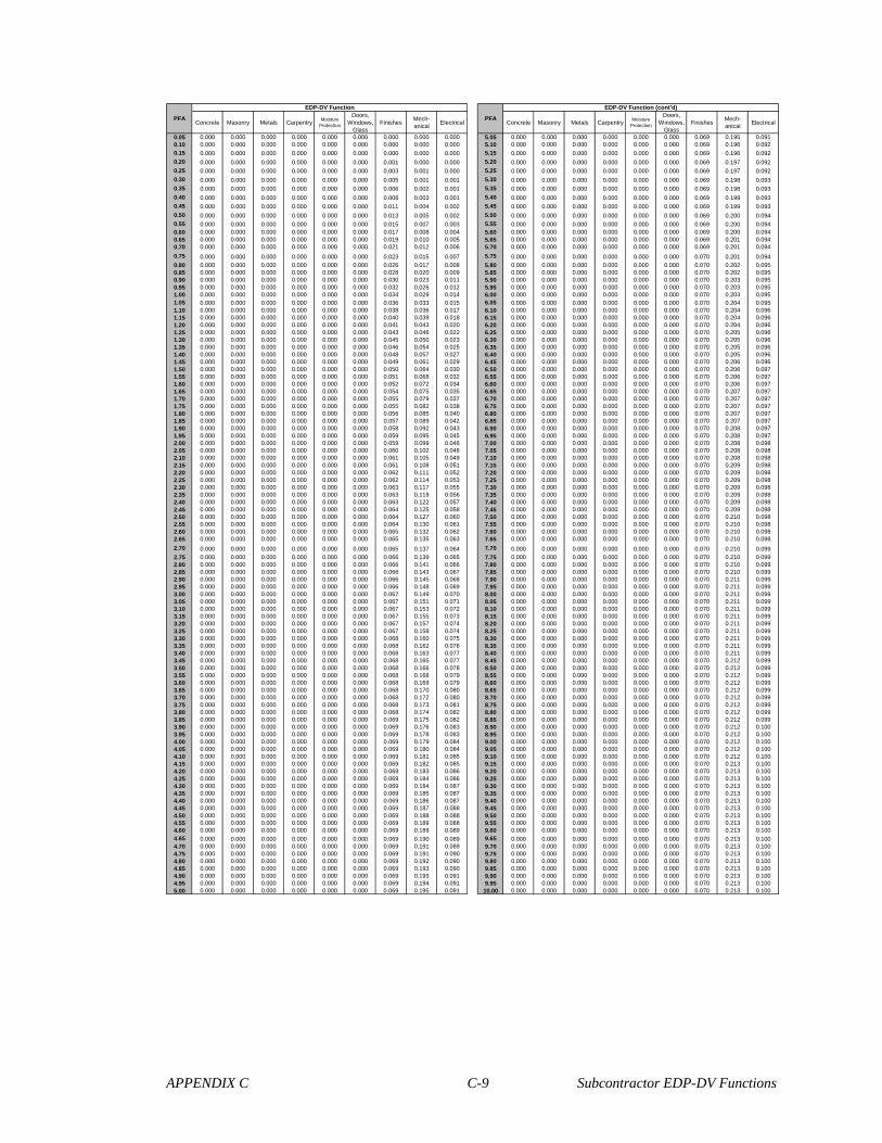
APPENDIX C C-9 Subcontractor EDP-DV Functions
Concrete Masonry Metals CarpentryMoisture
Protection
Doors, Windows,
GlassFinishes
Mech-anical
Electrical Concrete Masonry Metals CarpentryMoisture
Protection
Doors, Windows,
GlassFinishes
Mech-anical
Electrical
0.05 0.000 0.000 0.000 0.000 0.000 0.000 0.000 0.000 0.000 5.05 0.000 0.000 0.000 0.000 0.000 0.000 0.069 0.195 0.0910.10 0.000 0.000 0.000 0.000 0.000 0.000 0.000 0.000 0.000 5.10 0.000 0.000 0.000 0.000 0.000 0.000 0.069 0.196 0.092
0.15 0.000 0.000 0.000 0.000 0.000 0.000 0.000 0.000 0.000 5.15 0.000 0.000 0.000 0.000 0.000 0.000 0.069 0.196 0.092
0.20 0.000 0.000 0.000 0.000 0.000 0.000 0.001 0.000 0.000 5.20 0.000 0.000 0.000 0.000 0.000 0.000 0.069 0.197 0.092
0.25 0.000 0.000 0.000 0.000 0.000 0.000 0.003 0.001 0.000 5.25 0.000 0.000 0.000 0.000 0.000 0.000 0.069 0.197 0.092
0.30 0.000 0.000 0.000 0.000 0.000 0.000 0.005 0.001 0.001 5.30 0.000 0.000 0.000 0.000 0.000 0.000 0.069 0.198 0.093
0.35 0.000 0.000 0.000 0.000 0.000 0.000 0.006 0.002 0.001 5.35 0.000 0.000 0.000 0.000 0.000 0.000 0.069 0.198 0.093
0.40 0.000 0.000 0.000 0.000 0.000 0.000 0.008 0.003 0.001 5.40 0.000 0.000 0.000 0.000 0.000 0.000 0.069 0.199 0.093
0.45 0.000 0.000 0.000 0.000 0.000 0.000 0.011 0.004 0.002 5.45 0.000 0.000 0.000 0.000 0.000 0.000 0.069 0.199 0.093
0.50 0.000 0.000 0.000 0.000 0.000 0.000 0.013 0.005 0.002 5.50 0.000 0.000 0.000 0.000 0.000 0.000 0.069 0.200 0.094
0.55 0.000 0.000 0.000 0.000 0.000 0.000 0.015 0.007 0.003 5.55 0.000 0.000 0.000 0.000 0.000 0.000 0.069 0.200 0.0940.60 0.000 0.000 0.000 0.000 0.000 0.000 0.017 0.008 0.004 5.60 0.000 0.000 0.000 0.000 0.000 0.000 0.069 0.200 0.0940.65 0.000 0.000 0.000 0.000 0.000 0.000 0.019 0.010 0.005 5.65 0.000 0.000 0.000 0.000 0.000 0.000 0.069 0.201 0.0940.70 0.000 0.000 0.000 0.000 0.000 0.000 0.021 0.012 0.006 5.70 0.000 0.000 0.000 0.000 0.000 0.000 0.069 0.201 0.094
0.75 0.000 0.000 0.000 0.000 0.000 0.000 0.023 0.015 0.007 5.75 0.000 0.000 0.000 0.000 0.000 0.000 0.070 0.201 0.094
0.80 0.000 0.000 0.000 0.000 0.000 0.000 0.026 0.017 0.008 5.80 0.000 0.000 0.000 0.000 0.000 0.000 0.070 0.202 0.0950.85 0.000 0.000 0.000 0.000 0.000 0.000 0.028 0.020 0.009 5.85 0.000 0.000 0.000 0.000 0.000 0.000 0.070 0.202 0.0950.90 0.000 0.000 0.000 0.000 0.000 0.000 0.030 0.023 0.011 5.90 0.000 0.000 0.000 0.000 0.000 0.000 0.070 0.203 0.0950.95 0.000 0.000 0.000 0.000 0.000 0.000 0.032 0.026 0.012 5.95 0.000 0.000 0.000 0.000 0.000 0.000 0.070 0.203 0.0951.00 0.000 0.000 0.000 0.000 0.000 0.000 0.034 0.029 0.014 6.00 0.000 0.000 0.000 0.000 0.000 0.000 0.070 0.203 0.0951.05 0.000 0.000 0.000 0.000 0.000 0.000 0.036 0.033 0.015 6.05 0.000 0.000 0.000 0.000 0.000 0.000 0.070 0.204 0.0951.10 0.000 0.000 0.000 0.000 0.000 0.000 0.038 0.036 0.017 6.10 0.000 0.000 0.000 0.000 0.000 0.000 0.070 0.204 0.0961.15 0.000 0.000 0.000 0.000 0.000 0.000 0.040 0.039 0.018 6.15 0.000 0.000 0.000 0.000 0.000 0.000 0.070 0.204 0.0961.20 0.000 0.000 0.000 0.000 0.000 0.000 0.041 0.043 0.020 6.20 0.000 0.000 0.000 0.000 0.000 0.000 0.070 0.204 0.0961.25 0.000 0.000 0.000 0.000 0.000 0.000 0.043 0.046 0.022 6.25 0.000 0.000 0.000 0.000 0.000 0.000 0.070 0.205 0.0961.30 0.000 0.000 0.000 0.000 0.000 0.000 0.045 0.050 0.023 6.30 0.000 0.000 0.000 0.000 0.000 0.000 0.070 0.205 0.0961.35 0.000 0.000 0.000 0.000 0.000 0.000 0.046 0.054 0.025 6.35 0.000 0.000 0.000 0.000 0.000 0.000 0.070 0.205 0.0961.40 0.000 0.000 0.000 0.000 0.000 0.000 0.048 0.057 0.027 6.40 0.000 0.000 0.000 0.000 0.000 0.000 0.070 0.205 0.0961.45 0.000 0.000 0.000 0.000 0.000 0.000 0.049 0.061 0.029 6.45 0.000 0.000 0.000 0.000 0.000 0.000 0.070 0.206 0.0961.50 0.000 0.000 0.000 0.000 0.000 0.000 0.050 0.064 0.030 6.50 0.000 0.000 0.000 0.000 0.000 0.000 0.070 0.206 0.0971.55 0.000 0.000 0.000 0.000 0.000 0.000 0.051 0.068 0.032 6.55 0.000 0.000 0.000 0.000 0.000 0.000 0.070 0.206 0.0971.60 0.000 0.000 0.000 0.000 0.000 0.000 0.052 0.072 0.034 6.60 0.000 0.000 0.000 0.000 0.000 0.000 0.070 0.206 0.0971.65 0.000 0.000 0.000 0.000 0.000 0.000 0.054 0.075 0.035 6.65 0.000 0.000 0.000 0.000 0.000 0.000 0.070 0.207 0.0971.70 0.000 0.000 0.000 0.000 0.000 0.000 0.055 0.079 0.037 6.70 0.000 0.000 0.000 0.000 0.000 0.000 0.070 0.207 0.0971.75 0.000 0.000 0.000 0.000 0.000 0.000 0.055 0.082 0.038 6.75 0.000 0.000 0.000 0.000 0.000 0.000 0.070 0.207 0.0971.80 0.000 0.000 0.000 0.000 0.000 0.000 0.056 0.085 0.040 6.80 0.000 0.000 0.000 0.000 0.000 0.000 0.070 0.207 0.0971.85 0.000 0.000 0.000 0.000 0.000 0.000 0.057 0.089 0.042 6.85 0.000 0.000 0.000 0.000 0.000 0.000 0.070 0.207 0.0971.90 0.000 0.000 0.000 0.000 0.000 0.000 0.058 0.092 0.043 6.90 0.000 0.000 0.000 0.000 0.000 0.000 0.070 0.208 0.0971.95 0.000 0.000 0.000 0.000 0.000 0.000 0.059 0.095 0.045 6.95 0.000 0.000 0.000 0.000 0.000 0.000 0.070 0.208 0.0972.00 0.000 0.000 0.000 0.000 0.000 0.000 0.059 0.099 0.046 7.00 0.000 0.000 0.000 0.000 0.000 0.000 0.070 0.208 0.0982.05 0.000 0.000 0.000 0.000 0.000 0.000 0.060 0.102 0.048 7.05 0.000 0.000 0.000 0.000 0.000 0.000 0.070 0.208 0.0982.10 0.000 0.000 0.000 0.000 0.000 0.000 0.061 0.105 0.049 7.10 0.000 0.000 0.000 0.000 0.000 0.000 0.070 0.208 0.0982.15 0.000 0.000 0.000 0.000 0.000 0.000 0.061 0.108 0.051 7.15 0.000 0.000 0.000 0.000 0.000 0.000 0.070 0.209 0.0982.20 0.000 0.000 0.000 0.000 0.000 0.000 0.062 0.111 0.052 7.20 0.000 0.000 0.000 0.000 0.000 0.000 0.070 0.209 0.0982.25 0.000 0.000 0.000 0.000 0.000 0.000 0.062 0.114 0.053 7.25 0.000 0.000 0.000 0.000 0.000 0.000 0.070 0.209 0.0982.30 0.000 0.000 0.000 0.000 0.000 0.000 0.063 0.117 0.055 7.30 0.000 0.000 0.000 0.000 0.000 0.000 0.070 0.209 0.0982.35 0.000 0.000 0.000 0.000 0.000 0.000 0.063 0.119 0.056 7.35 0.000 0.000 0.000 0.000 0.000 0.000 0.070 0.209 0.0982.40 0.000 0.000 0.000 0.000 0.000 0.000 0.063 0.122 0.057 7.40 0.000 0.000 0.000 0.000 0.000 0.000 0.070 0.209 0.0982.45 0.000 0.000 0.000 0.000 0.000 0.000 0.064 0.125 0.058 7.45 0.000 0.000 0.000 0.000 0.000 0.000 0.070 0.209 0.0982.50 0.000 0.000 0.000 0.000 0.000 0.000 0.064 0.127 0.060 7.50 0.000 0.000 0.000 0.000 0.000 0.000 0.070 0.210 0.0982.55 0.000 0.000 0.000 0.000 0.000 0.000 0.064 0.130 0.061 7.55 0.000 0.000 0.000 0.000 0.000 0.000 0.070 0.210 0.0982.60 0.000 0.000 0.000 0.000 0.000 0.000 0.065 0.132 0.062 7.60 0.000 0.000 0.000 0.000 0.000 0.000 0.070 0.210 0.0982.65 0.000 0.000 0.000 0.000 0.000 0.000 0.065 0.135 0.063 7.65 0.000 0.000 0.000 0.000 0.000 0.000 0.070 0.210 0.098
2.70 0.000 0.000 0.000 0.000 0.000 0.000 0.065 0.137 0.064 7.70 0.000 0.000 0.000 0.000 0.000 0.000 0.070 0.210 0.099
2.75 0.000 0.000 0.000 0.000 0.000 0.000 0.066 0.139 0.065 7.75 0.000 0.000 0.000 0.000 0.000 0.000 0.070 0.210 0.0992.80 0.000 0.000 0.000 0.000 0.000 0.000 0.066 0.141 0.066 7.80 0.000 0.000 0.000 0.000 0.000 0.000 0.070 0.210 0.0992.85 0.000 0.000 0.000 0.000 0.000 0.000 0.066 0.143 0.067 7.85 0.000 0.000 0.000 0.000 0.000 0.000 0.070 0.210 0.0992.90 0.000 0.000 0.000 0.000 0.000 0.000 0.066 0.145 0.068 7.90 0.000 0.000 0.000 0.000 0.000 0.000 0.070 0.211 0.0992.95 0.000 0.000 0.000 0.000 0.000 0.000 0.066 0.148 0.069 7.95 0.000 0.000 0.000 0.000 0.000 0.000 0.070 0.211 0.0993.00 0.000 0.000 0.000 0.000 0.000 0.000 0.067 0.149 0.070 8.00 0.000 0.000 0.000 0.000 0.000 0.000 0.070 0.211 0.0993.05 0.000 0.000 0.000 0.000 0.000 0.000 0.067 0.151 0.071 8.05 0.000 0.000 0.000 0.000 0.000 0.000 0.070 0.211 0.0993.10 0.000 0.000 0.000 0.000 0.000 0.000 0.067 0.153 0.072 8.10 0.000 0.000 0.000 0.000 0.000 0.000 0.070 0.211 0.0993.15 0.000 0.000 0.000 0.000 0.000 0.000 0.067 0.155 0.073 8.15 0.000 0.000 0.000 0.000 0.000 0.000 0.070 0.211 0.0993.20 0.000 0.000 0.000 0.000 0.000 0.000 0.067 0.157 0.074 8.20 0.000 0.000 0.000 0.000 0.000 0.000 0.070 0.211 0.0993.25 0.000 0.000 0.000 0.000 0.000 0.000 0.067 0.158 0.074 8.25 0.000 0.000 0.000 0.000 0.000 0.000 0.070 0.211 0.0993.30 0.000 0.000 0.000 0.000 0.000 0.000 0.068 0.160 0.075 8.30 0.000 0.000 0.000 0.000 0.000 0.000 0.070 0.211 0.0993.35 0.000 0.000 0.000 0.000 0.000 0.000 0.068 0.162 0.076 8.35 0.000 0.000 0.000 0.000 0.000 0.000 0.070 0.211 0.0993.40 0.000 0.000 0.000 0.000 0.000 0.000 0.068 0.163 0.077 8.40 0.000 0.000 0.000 0.000 0.000 0.000 0.070 0.211 0.0993.45 0.000 0.000 0.000 0.000 0.000 0.000 0.068 0.165 0.077 8.45 0.000 0.000 0.000 0.000 0.000 0.000 0.070 0.212 0.0993.50 0.000 0.000 0.000 0.000 0.000 0.000 0.068 0.166 0.078 8.50 0.000 0.000 0.000 0.000 0.000 0.000 0.070 0.212 0.0993.55 0.000 0.000 0.000 0.000 0.000 0.000 0.068 0.168 0.079 8.55 0.000 0.000 0.000 0.000 0.000 0.000 0.070 0.212 0.0993.60 0.000 0.000 0.000 0.000 0.000 0.000 0.068 0.169 0.079 8.60 0.000 0.000 0.000 0.000 0.000 0.000 0.070 0.212 0.0993.65 0.000 0.000 0.000 0.000 0.000 0.000 0.068 0.170 0.080 8.65 0.000 0.000 0.000 0.000 0.000 0.000 0.070 0.212 0.0993.70 0.000 0.000 0.000 0.000 0.000 0.000 0.068 0.172 0.080 8.70 0.000 0.000 0.000 0.000 0.000 0.000 0.070 0.212 0.0993.75 0.000 0.000 0.000 0.000 0.000 0.000 0.068 0.173 0.081 8.75 0.000 0.000 0.000 0.000 0.000 0.000 0.070 0.212 0.0993.80 0.000 0.000 0.000 0.000 0.000 0.000 0.068 0.174 0.082 8.80 0.000 0.000 0.000 0.000 0.000 0.000 0.070 0.212 0.0993.85 0.000 0.000 0.000 0.000 0.000 0.000 0.069 0.175 0.082 8.85 0.000 0.000 0.000 0.000 0.000 0.000 0.070 0.212 0.0993.90 0.000 0.000 0.000 0.000 0.000 0.000 0.069 0.176 0.083 8.90 0.000 0.000 0.000 0.000 0.000 0.000 0.070 0.212 0.1003.95 0.000 0.000 0.000 0.000 0.000 0.000 0.069 0.178 0.083 8.95 0.000 0.000 0.000 0.000 0.000 0.000 0.070 0.212 0.1004.00 0.000 0.000 0.000 0.000 0.000 0.000 0.069 0.179 0.084 9.00 0.000 0.000 0.000 0.000 0.000 0.000 0.070 0.212 0.1004.05 0.000 0.000 0.000 0.000 0.000 0.000 0.069 0.180 0.084 9.05 0.000 0.000 0.000 0.000 0.000 0.000 0.070 0.212 0.1004.10 0.000 0.000 0.000 0.000 0.000 0.000 0.069 0.181 0.085 9.10 0.000 0.000 0.000 0.000 0.000 0.000 0.070 0.212 0.1004.15 0.000 0.000 0.000 0.000 0.000 0.000 0.069 0.182 0.085 9.15 0.000 0.000 0.000 0.000 0.000 0.000 0.070 0.213 0.1004.20 0.000 0.000 0.000 0.000 0.000 0.000 0.069 0.183 0.086 9.20 0.000 0.000 0.000 0.000 0.000 0.000 0.070 0.213 0.1004.25 0.000 0.000 0.000 0.000 0.000 0.000 0.069 0.184 0.086 9.25 0.000 0.000 0.000 0.000 0.000 0.000 0.070 0.213 0.1004.30 0.000 0.000 0.000 0.000 0.000 0.000 0.069 0.184 0.087 9.30 0.000 0.000 0.000 0.000 0.000 0.000 0.070 0.213 0.1004.35 0.000 0.000 0.000 0.000 0.000 0.000 0.069 0.185 0.087 9.35 0.000 0.000 0.000 0.000 0.000 0.000 0.070 0.213 0.1004.40 0.000 0.000 0.000 0.000 0.000 0.000 0.069 0.186 0.087 9.40 0.000 0.000 0.000 0.000 0.000 0.000 0.070 0.213 0.1004.45 0.000 0.000 0.000 0.000 0.000 0.000 0.069 0.187 0.088 9.45 0.000 0.000 0.000 0.000 0.000 0.000 0.070 0.213 0.1004.50 0.000 0.000 0.000 0.000 0.000 0.000 0.069 0.188 0.088 9.50 0.000 0.000 0.000 0.000 0.000 0.000 0.070 0.213 0.1004.55 0.000 0.000 0.000 0.000 0.000 0.000 0.069 0.189 0.088 9.55 0.000 0.000 0.000 0.000 0.000 0.000 0.070 0.213 0.1004.60 0.000 0.000 0.000 0.000 0.000 0.000 0.069 0.189 0.089 9.60 0.000 0.000 0.000 0.000 0.000 0.000 0.070 0.213 0.1004.65 0.000 0.000 0.000 0.000 0.000 0.000 0.069 0.190 0.089 9.65 0.000 0.000 0.000 0.000 0.000 0.000 0.070 0.213 0.1004.70 0.000 0.000 0.000 0.000 0.000 0.000 0.069 0.191 0.089 9.70 0.000 0.000 0.000 0.000 0.000 0.000 0.070 0.213 0.1004.75 0.000 0.000 0.000 0.000 0.000 0.000 0.069 0.191 0.090 9.75 0.000 0.000 0.000 0.000 0.000 0.000 0.070 0.213 0.1004.80 0.000 0.000 0.000 0.000 0.000 0.000 0.069 0.192 0.090 9.80 0.000 0.000 0.000 0.000 0.000 0.000 0.070 0.213 0.1004.85 0.000 0.000 0.000 0.000 0.000 0.000 0.069 0.193 0.090 9.85 0.000 0.000 0.000 0.000 0.000 0.000 0.070 0.213 0.1004.90 0.000 0.000 0.000 0.000 0.000 0.000 0.069 0.193 0.091 9.90 0.000 0.000 0.000 0.000 0.000 0.000 0.070 0.213 0.1004.95 0.000 0.000 0.000 0.000 0.000 0.000 0.069 0.194 0.091 9.95 0.000 0.000 0.000 0.000 0.000 0.000 0.070 0.213 0.1005.00 0.000 0.000 0.000 0.000 0.000 0.000 0.069 0.195 0.091 10.00 0.000 0.000 0.000 0.000 0.000 0.000 0.070 0.213 0.100
EDP-DV Function
PFA PFA
EDP-DV Function (cont'd)

APPENDIX C C-10 Subcontractor EDP-DV Functions
Subcontractor EDP-DV Functions
Building Height: Low-rise (1 to 5 stories)
Strucutral Material: Ductile reinforced-concrete
Structural System: Perimeter moment-frame
Occupancy: Office
Floor Type: Typical Floor
Functions for PFA = 0 to 5g
Functions for PFA = 0 to 10g
(Data points on following page)
0.00
0.05
0.10
0.15
0.20
0.25
0.0 2.0 4.0 6.0 8.0 10.0
PFA [g]
E( L | PFA )
Finishes
Mechanical
Electrical
0.00
0.05
0.10
0.15
0.20
0.25
0.0 1.0 2.0 3.0 4.0 5.0
PFA [g]
E( L | PFA )
Finishes
Mechanical
Electrical
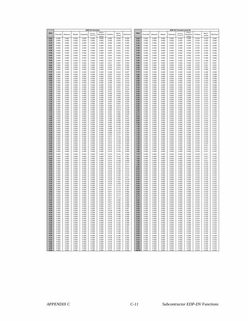
APPENDIX C C-11 Subcontractor EDP-DV Functions
Concrete Masonry Metals CarpentryMoisture
Protection
Doors, Windows,
GlassFinishes
Mech-anical
Electrical Concrete Masonry Metals CarpentryMoisture
Protection
Doors, Windows,
GlassFinishes
Mech-anical
Electrical
0.05 0.000 0.000 0.000 0.000 0.000 0.000 0.000 0.000 0.000 5.05 0.000 0.000 0.000 0.000 0.000 0.000 0.078 0.202 0.0950.10 0.000 0.000 0.000 0.000 0.000 0.000 0.000 0.000 0.000 5.10 0.000 0.000 0.000 0.000 0.000 0.000 0.078 0.202 0.095
0.15 0.000 0.000 0.000 0.000 0.000 0.000 0.000 0.000 0.000 5.15 0.000 0.000 0.000 0.000 0.000 0.000 0.078 0.203 0.095
0.20 0.000 0.000 0.000 0.000 0.000 0.000 0.001 0.000 0.000 5.20 0.000 0.000 0.000 0.000 0.000 0.000 0.078 0.203 0.095
0.25 0.000 0.000 0.000 0.000 0.000 0.000 0.003 0.001 0.000 5.25 0.000 0.000 0.000 0.000 0.000 0.000 0.078 0.204 0.096
0.30 0.000 0.000 0.000 0.000 0.000 0.000 0.005 0.001 0.001 5.30 0.000 0.000 0.000 0.000 0.000 0.000 0.078 0.204 0.096
0.35 0.000 0.000 0.000 0.000 0.000 0.000 0.007 0.002 0.001 5.35 0.000 0.000 0.000 0.000 0.000 0.000 0.078 0.205 0.096
0.40 0.000 0.000 0.000 0.000 0.000 0.000 0.010 0.003 0.001 5.40 0.000 0.000 0.000 0.000 0.000 0.000 0.078 0.205 0.096
0.45 0.000 0.000 0.000 0.000 0.000 0.000 0.012 0.004 0.002 5.45 0.000 0.000 0.000 0.000 0.000 0.000 0.078 0.206 0.096
0.50 0.000 0.000 0.000 0.000 0.000 0.000 0.014 0.005 0.003 5.50 0.000 0.000 0.000 0.000 0.000 0.000 0.078 0.206 0.097
0.55 0.000 0.000 0.000 0.000 0.000 0.000 0.017 0.007 0.003 5.55 0.000 0.000 0.000 0.000 0.000 0.000 0.078 0.207 0.0970.60 0.000 0.000 0.000 0.000 0.000 0.000 0.019 0.009 0.004 5.60 0.000 0.000 0.000 0.000 0.000 0.000 0.078 0.207 0.0970.65 0.000 0.000 0.000 0.000 0.000 0.000 0.021 0.011 0.005 5.65 0.000 0.000 0.000 0.000 0.000 0.000 0.078 0.207 0.0970.70 0.000 0.000 0.000 0.000 0.000 0.000 0.024 0.013 0.006 5.70 0.000 0.000 0.000 0.000 0.000 0.000 0.078 0.208 0.097
0.75 0.000 0.000 0.000 0.000 0.000 0.000 0.026 0.015 0.007 5.75 0.000 0.000 0.000 0.000 0.000 0.000 0.078 0.208 0.098
0.80 0.000 0.000 0.000 0.000 0.000 0.000 0.029 0.018 0.008 5.80 0.000 0.000 0.000 0.000 0.000 0.000 0.078 0.209 0.0980.85 0.000 0.000 0.000 0.000 0.000 0.000 0.031 0.021 0.010 5.85 0.000 0.000 0.000 0.000 0.000 0.000 0.078 0.209 0.0980.90 0.000 0.000 0.000 0.000 0.000 0.000 0.034 0.024 0.011 5.90 0.000 0.000 0.000 0.000 0.000 0.000 0.078 0.209 0.0980.95 0.000 0.000 0.000 0.000 0.000 0.000 0.036 0.027 0.013 5.95 0.000 0.000 0.000 0.000 0.000 0.000 0.078 0.210 0.0981.00 0.000 0.000 0.000 0.000 0.000 0.000 0.038 0.030 0.014 6.00 0.000 0.000 0.000 0.000 0.000 0.000 0.078 0.210 0.0981.05 0.000 0.000 0.000 0.000 0.000 0.000 0.041 0.034 0.016 6.05 0.000 0.000 0.000 0.000 0.000 0.000 0.078 0.210 0.0991.10 0.000 0.000 0.000 0.000 0.000 0.000 0.043 0.037 0.017 6.10 0.000 0.000 0.000 0.000 0.000 0.000 0.078 0.211 0.0991.15 0.000 0.000 0.000 0.000 0.000 0.000 0.045 0.041 0.019 6.15 0.000 0.000 0.000 0.000 0.000 0.000 0.078 0.211 0.0991.20 0.000 0.000 0.000 0.000 0.000 0.000 0.047 0.044 0.021 6.20 0.000 0.000 0.000 0.000 0.000 0.000 0.078 0.211 0.0991.25 0.000 0.000 0.000 0.000 0.000 0.000 0.049 0.048 0.022 6.25 0.000 0.000 0.000 0.000 0.000 0.000 0.078 0.211 0.0991.30 0.000 0.000 0.000 0.000 0.000 0.000 0.050 0.052 0.024 6.30 0.000 0.000 0.000 0.000 0.000 0.000 0.078 0.212 0.0991.35 0.000 0.000 0.000 0.000 0.000 0.000 0.052 0.055 0.026 6.35 0.000 0.000 0.000 0.000 0.000 0.000 0.078 0.212 0.0991.40 0.000 0.000 0.000 0.000 0.000 0.000 0.054 0.059 0.028 6.40 0.000 0.000 0.000 0.000 0.000 0.000 0.078 0.212 0.1001.45 0.000 0.000 0.000 0.000 0.000 0.000 0.055 0.063 0.029 6.45 0.000 0.000 0.000 0.000 0.000 0.000 0.078 0.213 0.1001.50 0.000 0.000 0.000 0.000 0.000 0.000 0.057 0.067 0.031 6.50 0.000 0.000 0.000 0.000 0.000 0.000 0.078 0.213 0.1001.55 0.000 0.000 0.000 0.000 0.000 0.000 0.058 0.070 0.033 6.55 0.000 0.000 0.000 0.000 0.000 0.000 0.078 0.213 0.1001.60 0.000 0.000 0.000 0.000 0.000 0.000 0.059 0.074 0.035 6.60 0.000 0.000 0.000 0.000 0.000 0.000 0.078 0.213 0.1001.65 0.000 0.000 0.000 0.000 0.000 0.000 0.060 0.078 0.036 6.65 0.000 0.000 0.000 0.000 0.000 0.000 0.078 0.213 0.1001.70 0.000 0.000 0.000 0.000 0.000 0.000 0.061 0.081 0.038 6.70 0.000 0.000 0.000 0.000 0.000 0.000 0.078 0.214 0.1001.75 0.000 0.000 0.000 0.000 0.000 0.000 0.062 0.085 0.040 6.75 0.000 0.000 0.000 0.000 0.000 0.000 0.078 0.214 0.1001.80 0.000 0.000 0.000 0.000 0.000 0.000 0.063 0.088 0.041 6.80 0.000 0.000 0.000 0.000 0.000 0.000 0.078 0.214 0.1001.85 0.000 0.000 0.000 0.000 0.000 0.000 0.064 0.092 0.043 6.85 0.000 0.000 0.000 0.000 0.000 0.000 0.078 0.214 0.1011.90 0.000 0.000 0.000 0.000 0.000 0.000 0.065 0.095 0.045 6.90 0.000 0.000 0.000 0.000 0.000 0.000 0.078 0.215 0.1011.95 0.000 0.000 0.000 0.000 0.000 0.000 0.066 0.099 0.046 6.95 0.000 0.000 0.000 0.000 0.000 0.000 0.078 0.215 0.1012.00 0.000 0.000 0.000 0.000 0.000 0.000 0.067 0.102 0.048 7.00 0.000 0.000 0.000 0.000 0.000 0.000 0.078 0.215 0.1012.05 0.000 0.000 0.000 0.000 0.000 0.000 0.068 0.105 0.049 7.05 0.000 0.000 0.000 0.000 0.000 0.000 0.078 0.215 0.1012.10 0.000 0.000 0.000 0.000 0.000 0.000 0.068 0.108 0.051 7.10 0.000 0.000 0.000 0.000 0.000 0.000 0.078 0.215 0.1012.15 0.000 0.000 0.000 0.000 0.000 0.000 0.069 0.111 0.052 7.15 0.000 0.000 0.000 0.000 0.000 0.000 0.078 0.215 0.1012.20 0.000 0.000 0.000 0.000 0.000 0.000 0.069 0.115 0.054 7.20 0.000 0.000 0.000 0.000 0.000 0.000 0.078 0.216 0.1012.25 0.000 0.000 0.000 0.000 0.000 0.000 0.070 0.117 0.055 7.25 0.000 0.000 0.000 0.000 0.000 0.000 0.078 0.216 0.1012.30 0.000 0.000 0.000 0.000 0.000 0.000 0.071 0.120 0.056 7.30 0.000 0.000 0.000 0.000 0.000 0.000 0.078 0.216 0.1012.35 0.000 0.000 0.000 0.000 0.000 0.000 0.071 0.123 0.058 7.35 0.000 0.000 0.000 0.000 0.000 0.000 0.078 0.216 0.1012.40 0.000 0.000 0.000 0.000 0.000 0.000 0.071 0.126 0.059 7.40 0.000 0.000 0.000 0.000 0.000 0.000 0.078 0.216 0.1012.45 0.000 0.000 0.000 0.000 0.000 0.000 0.072 0.129 0.060 7.45 0.000 0.000 0.000 0.000 0.000 0.000 0.078 0.216 0.1012.50 0.000 0.000 0.000 0.000 0.000 0.000 0.072 0.131 0.062 7.50 0.000 0.000 0.000 0.000 0.000 0.000 0.078 0.217 0.1022.55 0.000 0.000 0.000 0.000 0.000 0.000 0.073 0.134 0.063 7.55 0.000 0.000 0.000 0.000 0.000 0.000 0.078 0.217 0.1022.60 0.000 0.000 0.000 0.000 0.000 0.000 0.073 0.137 0.064 7.60 0.000 0.000 0.000 0.000 0.000 0.000 0.078 0.217 0.1022.65 0.000 0.000 0.000 0.000 0.000 0.000 0.073 0.139 0.065 7.65 0.000 0.000 0.000 0.000 0.000 0.000 0.078 0.217 0.102
2.70 0.000 0.000 0.000 0.000 0.000 0.000 0.074 0.141 0.066 7.70 0.000 0.000 0.000 0.000 0.000 0.000 0.078 0.217 0.102
2.75 0.000 0.000 0.000 0.000 0.000 0.000 0.074 0.144 0.067 7.75 0.000 0.000 0.000 0.000 0.000 0.000 0.078 0.217 0.1022.80 0.000 0.000 0.000 0.000 0.000 0.000 0.074 0.146 0.068 7.80 0.000 0.000 0.000 0.000 0.000 0.000 0.078 0.217 0.1022.85 0.000 0.000 0.000 0.000 0.000 0.000 0.074 0.148 0.069 7.85 0.000 0.000 0.000 0.000 0.000 0.000 0.078 0.217 0.1022.90 0.000 0.000 0.000 0.000 0.000 0.000 0.075 0.150 0.070 7.90 0.000 0.000 0.000 0.000 0.000 0.000 0.078 0.218 0.1022.95 0.000 0.000 0.000 0.000 0.000 0.000 0.075 0.152 0.071 7.95 0.000 0.000 0.000 0.000 0.000 0.000 0.078 0.218 0.1023.00 0.000 0.000 0.000 0.000 0.000 0.000 0.075 0.154 0.072 8.00 0.000 0.000 0.000 0.000 0.000 0.000 0.078 0.218 0.1023.05 0.000 0.000 0.000 0.000 0.000 0.000 0.075 0.156 0.073 8.05 0.000 0.000 0.000 0.000 0.000 0.000 0.078 0.218 0.1023.10 0.000 0.000 0.000 0.000 0.000 0.000 0.076 0.158 0.074 8.10 0.000 0.000 0.000 0.000 0.000 0.000 0.078 0.218 0.1023.15 0.000 0.000 0.000 0.000 0.000 0.000 0.076 0.160 0.075 8.15 0.000 0.000 0.000 0.000 0.000 0.000 0.078 0.218 0.1023.20 0.000 0.000 0.000 0.000 0.000 0.000 0.076 0.162 0.076 8.20 0.000 0.000 0.000 0.000 0.000 0.000 0.078 0.218 0.1023.25 0.000 0.000 0.000 0.000 0.000 0.000 0.076 0.164 0.077 8.25 0.000 0.000 0.000 0.000 0.000 0.000 0.078 0.218 0.1023.30 0.000 0.000 0.000 0.000 0.000 0.000 0.076 0.165 0.078 8.30 0.000 0.000 0.000 0.000 0.000 0.000 0.078 0.218 0.1023.35 0.000 0.000 0.000 0.000 0.000 0.000 0.076 0.167 0.078 8.35 0.000 0.000 0.000 0.000 0.000 0.000 0.078 0.218 0.1023.40 0.000 0.000 0.000 0.000 0.000 0.000 0.076 0.169 0.079 8.40 0.000 0.000 0.000 0.000 0.000 0.000 0.079 0.219 0.1023.45 0.000 0.000 0.000 0.000 0.000 0.000 0.077 0.170 0.080 8.45 0.000 0.000 0.000 0.000 0.000 0.000 0.079 0.219 0.1033.50 0.000 0.000 0.000 0.000 0.000 0.000 0.077 0.172 0.081 8.50 0.000 0.000 0.000 0.000 0.000 0.000 0.079 0.219 0.1033.55 0.000 0.000 0.000 0.000 0.000 0.000 0.077 0.173 0.081 8.55 0.000 0.000 0.000 0.000 0.000 0.000 0.079 0.219 0.1033.60 0.000 0.000 0.000 0.000 0.000 0.000 0.077 0.175 0.082 8.60 0.000 0.000 0.000 0.000 0.000 0.000 0.079 0.219 0.1033.65 0.000 0.000 0.000 0.000 0.000 0.000 0.077 0.176 0.083 8.65 0.000 0.000 0.000 0.000 0.000 0.000 0.079 0.219 0.1033.70 0.000 0.000 0.000 0.000 0.000 0.000 0.077 0.177 0.083 8.70 0.000 0.000 0.000 0.000 0.000 0.000 0.079 0.219 0.1033.75 0.000 0.000 0.000 0.000 0.000 0.000 0.077 0.179 0.084 8.75 0.000 0.000 0.000 0.000 0.000 0.000 0.079 0.219 0.1033.80 0.000 0.000 0.000 0.000 0.000 0.000 0.077 0.180 0.084 8.80 0.000 0.000 0.000 0.000 0.000 0.000 0.079 0.219 0.1033.85 0.000 0.000 0.000 0.000 0.000 0.000 0.077 0.181 0.085 8.85 0.000 0.000 0.000 0.000 0.000 0.000 0.079 0.219 0.1033.90 0.000 0.000 0.000 0.000 0.000 0.000 0.077 0.182 0.086 8.90 0.000 0.000 0.000 0.000 0.000 0.000 0.079 0.219 0.1033.95 0.000 0.000 0.000 0.000 0.000 0.000 0.077 0.183 0.086 8.95 0.000 0.000 0.000 0.000 0.000 0.000 0.079 0.219 0.1034.00 0.000 0.000 0.000 0.000 0.000 0.000 0.077 0.185 0.087 9.00 0.000 0.000 0.000 0.000 0.000 0.000 0.079 0.219 0.1034.05 0.000 0.000 0.000 0.000 0.000 0.000 0.078 0.186 0.087 9.05 0.000 0.000 0.000 0.000 0.000 0.000 0.079 0.219 0.1034.10 0.000 0.000 0.000 0.000 0.000 0.000 0.078 0.187 0.088 9.10 0.000 0.000 0.000 0.000 0.000 0.000 0.079 0.220 0.1034.15 0.000 0.000 0.000 0.000 0.000 0.000 0.078 0.188 0.088 9.15 0.000 0.000 0.000 0.000 0.000 0.000 0.079 0.220 0.1034.20 0.000 0.000 0.000 0.000 0.000 0.000 0.078 0.189 0.089 9.20 0.000 0.000 0.000 0.000 0.000 0.000 0.079 0.220 0.1034.25 0.000 0.000 0.000 0.000 0.000 0.000 0.078 0.190 0.089 9.25 0.000 0.000 0.000 0.000 0.000 0.000 0.079 0.220 0.1034.30 0.000 0.000 0.000 0.000 0.000 0.000 0.078 0.191 0.089 9.30 0.000 0.000 0.000 0.000 0.000 0.000 0.079 0.220 0.1034.35 0.000 0.000 0.000 0.000 0.000 0.000 0.078 0.192 0.090 9.35 0.000 0.000 0.000 0.000 0.000 0.000 0.079 0.220 0.1034.40 0.000 0.000 0.000 0.000 0.000 0.000 0.078 0.192 0.090 9.40 0.000 0.000 0.000 0.000 0.000 0.000 0.079 0.220 0.1034.45 0.000 0.000 0.000 0.000 0.000 0.000 0.078 0.193 0.091 9.45 0.000 0.000 0.000 0.000 0.000 0.000 0.079 0.220 0.1034.50 0.000 0.000 0.000 0.000 0.000 0.000 0.078 0.194 0.091 9.50 0.000 0.000 0.000 0.000 0.000 0.000 0.079 0.220 0.1034.55 0.000 0.000 0.000 0.000 0.000 0.000 0.078 0.195 0.091 9.55 0.000 0.000 0.000 0.000 0.000 0.000 0.079 0.220 0.1034.60 0.000 0.000 0.000 0.000 0.000 0.000 0.078 0.196 0.092 9.60 0.000 0.000 0.000 0.000 0.000 0.000 0.079 0.220 0.1034.65 0.000 0.000 0.000 0.000 0.000 0.000 0.078 0.196 0.092 9.65 0.000 0.000 0.000 0.000 0.000 0.000 0.079 0.220 0.1034.70 0.000 0.000 0.000 0.000 0.000 0.000 0.078 0.197 0.092 9.70 0.000 0.000 0.000 0.000 0.000 0.000 0.079 0.220 0.1034.75 0.000 0.000 0.000 0.000 0.000 0.000 0.078 0.198 0.093 9.75 0.000 0.000 0.000 0.000 0.000 0.000 0.079 0.220 0.1034.80 0.000 0.000 0.000 0.000 0.000 0.000 0.078 0.198 0.093 9.80 0.000 0.000 0.000 0.000 0.000 0.000 0.079 0.220 0.1034.85 0.000 0.000 0.000 0.000 0.000 0.000 0.078 0.199 0.093 9.85 0.000 0.000 0.000 0.000 0.000 0.000 0.079 0.220 0.1034.90 0.000 0.000 0.000 0.000 0.000 0.000 0.078 0.200 0.094 9.90 0.000 0.000 0.000 0.000 0.000 0.000 0.079 0.220 0.1034.95 0.000 0.000 0.000 0.000 0.000 0.000 0.078 0.200 0.094 9.95 0.000 0.000 0.000 0.000 0.000 0.000 0.079 0.220 0.1035.00 0.000 0.000 0.000 0.000 0.000 0.000 0.078 0.201 0.094 10.00 0.000 0.000 0.000 0.000 0.000 0.000 0.079 0.220 0.103
EDP-DV Function
PFA PFA
EDP-DV Function (cont'd)
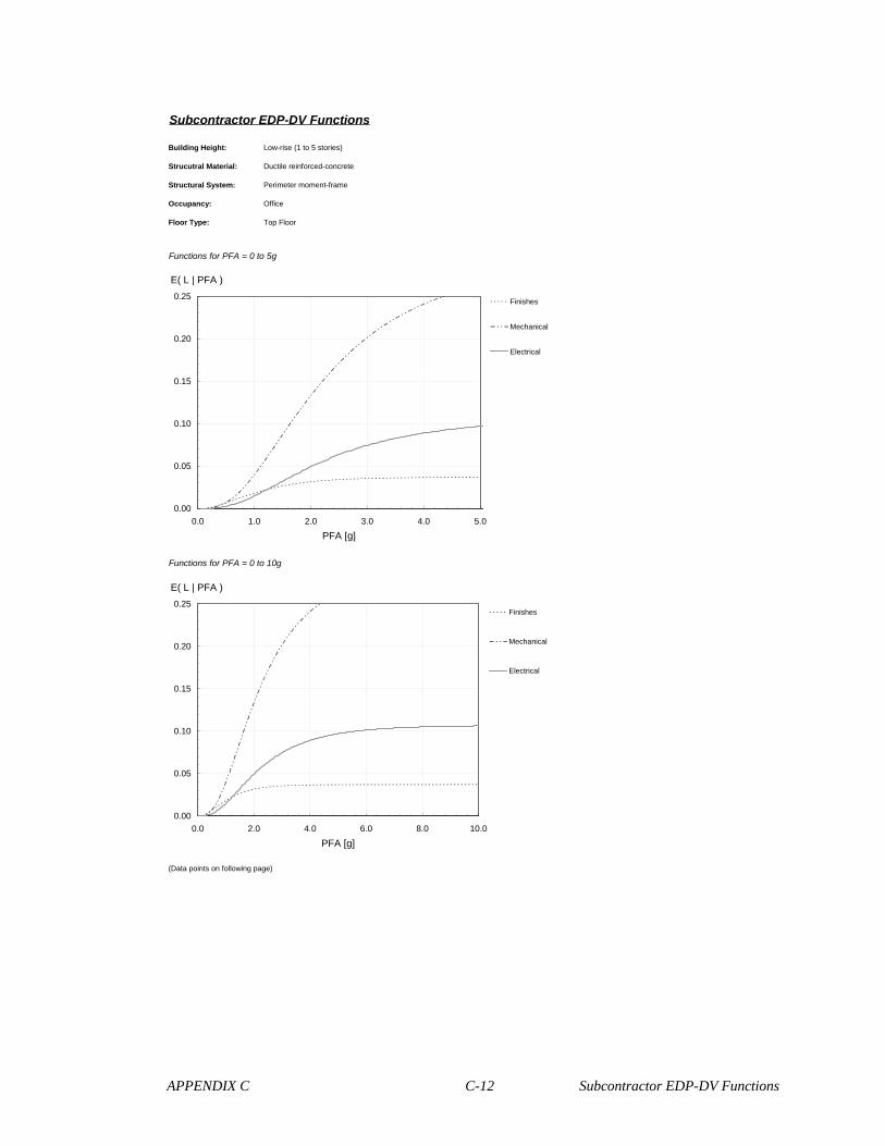
APPENDIX C C-12 Subcontractor EDP-DV Functions
Subcontractor EDP-DV Functions
Building Height: Low-rise (1 to 5 stories)
Strucutral Material: Ductile reinforced-concrete
Structural System: Perimeter moment-frame
Occupancy: Office
Floor Type: Top Floor
Functions for PFA = 0 to 5g
Functions for PFA = 0 to 10g
(Data points on following page)
0.00
0.05
0.10
0.15
0.20
0.25
0.0 2.0 4.0 6.0 8.0 10.0
PFA [g]
E( L | PFA )
Finishes
Mechanical
Electrical
0.00
0.05
0.10
0.15
0.20
0.25
0.0 1.0 2.0 3.0 4.0 5.0
PFA [g]
E( L | PFA )
Finishes
Mechanical
Electrical

APPENDIX C C-13 Subcontractor EDP-DV Functions
Concrete Masonry Metals CarpentryMoisture
Protection
Doors, Windows,
GlassFinishes
Mech-anical
Electrical Concrete Masonry Metals CarpentryMoisture
Protection
Doors, Windows,
GlassFinishes
Mech-anical
Electrical
0.05 0.000 0.000 0.000 0.000 0.000 0.000 0.000 0.000 0.000 5.05 0.000 0.000 0.000 0.000 0.000 0.000 0.037 0.263 0.0970.10 0.000 0.000 0.000 0.000 0.000 0.000 0.000 0.000 0.000 5.10 0.000 0.000 0.000 0.000 0.000 0.000 0.037 0.264 0.097
0.15 0.000 0.000 0.000 0.000 0.000 0.000 0.000 0.000 0.000 5.15 0.000 0.000 0.000 0.000 0.000 0.000 0.037 0.264 0.098
0.20 0.000 0.000 0.000 0.000 0.000 0.000 0.001 0.000 0.000 5.20 0.000 0.000 0.000 0.000 0.000 0.000 0.037 0.265 0.098
0.25 0.000 0.000 0.000 0.000 0.000 0.000 0.001 0.001 0.000 5.25 0.000 0.000 0.000 0.000 0.000 0.000 0.037 0.266 0.098
0.30 0.000 0.000 0.000 0.000 0.000 0.000 0.002 0.002 0.001 5.30 0.000 0.000 0.000 0.000 0.000 0.000 0.037 0.266 0.098
0.35 0.000 0.000 0.000 0.000 0.000 0.000 0.003 0.003 0.001 5.35 0.000 0.000 0.000 0.000 0.000 0.000 0.037 0.267 0.099
0.40 0.000 0.000 0.000 0.000 0.000 0.000 0.004 0.004 0.001 5.40 0.000 0.000 0.000 0.000 0.000 0.000 0.037 0.268 0.099
0.45 0.000 0.000 0.000 0.000 0.000 0.000 0.006 0.005 0.002 5.45 0.000 0.000 0.000 0.000 0.000 0.000 0.037 0.268 0.099
0.50 0.000 0.000 0.000 0.000 0.000 0.000 0.007 0.007 0.003 5.50 0.000 0.000 0.000 0.000 0.000 0.000 0.037 0.269 0.099
0.55 0.000 0.000 0.000 0.000 0.000 0.000 0.008 0.009 0.003 5.55 0.000 0.000 0.000 0.000 0.000 0.000 0.037 0.269 0.1000.60 0.000 0.000 0.000 0.000 0.000 0.000 0.009 0.011 0.004 5.60 0.000 0.000 0.000 0.000 0.000 0.000 0.037 0.270 0.1000.65 0.000 0.000 0.000 0.000 0.000 0.000 0.010 0.014 0.005 5.65 0.000 0.000 0.000 0.000 0.000 0.000 0.037 0.271 0.1000.70 0.000 0.000 0.000 0.000 0.000 0.000 0.011 0.017 0.006 5.70 0.000 0.000 0.000 0.000 0.000 0.000 0.037 0.271 0.100
0.75 0.000 0.000 0.000 0.000 0.000 0.000 0.012 0.020 0.007 5.75 0.000 0.000 0.000 0.000 0.000 0.000 0.037 0.272 0.100
0.80 0.000 0.000 0.000 0.000 0.000 0.000 0.014 0.023 0.009 5.80 0.000 0.000 0.000 0.000 0.000 0.000 0.037 0.272 0.1010.85 0.000 0.000 0.000 0.000 0.000 0.000 0.015 0.027 0.010 5.85 0.000 0.000 0.000 0.000 0.000 0.000 0.037 0.273 0.1010.90 0.000 0.000 0.000 0.000 0.000 0.000 0.016 0.031 0.011 5.90 0.000 0.000 0.000 0.000 0.000 0.000 0.037 0.273 0.1010.95 0.000 0.000 0.000 0.000 0.000 0.000 0.017 0.035 0.013 5.95 0.000 0.000 0.000 0.000 0.000 0.000 0.037 0.273 0.1011.00 0.000 0.000 0.000 0.000 0.000 0.000 0.018 0.039 0.015 6.00 0.000 0.000 0.000 0.000 0.000 0.000 0.037 0.274 0.1011.05 0.000 0.000 0.000 0.000 0.000 0.000 0.019 0.044 0.016 6.05 0.000 0.000 0.000 0.000 0.000 0.000 0.037 0.274 0.1011.10 0.000 0.000 0.000 0.000 0.000 0.000 0.020 0.048 0.018 6.10 0.000 0.000 0.000 0.000 0.000 0.000 0.037 0.275 0.1021.15 0.000 0.000 0.000 0.000 0.000 0.000 0.021 0.053 0.020 6.15 0.000 0.000 0.000 0.000 0.000 0.000 0.037 0.275 0.1021.20 0.000 0.000 0.000 0.000 0.000 0.000 0.022 0.058 0.021 6.20 0.000 0.000 0.000 0.000 0.000 0.000 0.037 0.276 0.1021.25 0.000 0.000 0.000 0.000 0.000 0.000 0.023 0.063 0.023 6.25 0.000 0.000 0.000 0.000 0.000 0.000 0.037 0.276 0.1021.30 0.000 0.000 0.000 0.000 0.000 0.000 0.024 0.067 0.025 6.30 0.000 0.000 0.000 0.000 0.000 0.000 0.037 0.276 0.1021.35 0.000 0.000 0.000 0.000 0.000 0.000 0.025 0.072 0.027 6.35 0.000 0.000 0.000 0.000 0.000 0.000 0.037 0.277 0.1021.40 0.000 0.000 0.000 0.000 0.000 0.000 0.025 0.077 0.028 6.40 0.000 0.000 0.000 0.000 0.000 0.000 0.037 0.277 0.1021.45 0.000 0.000 0.000 0.000 0.000 0.000 0.026 0.082 0.030 6.45 0.000 0.000 0.000 0.000 0.000 0.000 0.037 0.277 0.1021.50 0.000 0.000 0.000 0.000 0.000 0.000 0.027 0.087 0.032 6.50 0.000 0.000 0.000 0.000 0.000 0.000 0.037 0.278 0.1031.55 0.000 0.000 0.000 0.000 0.000 0.000 0.027 0.092 0.034 6.55 0.000 0.000 0.000 0.000 0.000 0.000 0.037 0.278 0.1031.60 0.000 0.000 0.000 0.000 0.000 0.000 0.028 0.096 0.036 6.60 0.000 0.000 0.000 0.000 0.000 0.000 0.037 0.278 0.1031.65 0.000 0.000 0.000 0.000 0.000 0.000 0.028 0.101 0.037 6.65 0.000 0.000 0.000 0.000 0.000 0.000 0.037 0.279 0.1031.70 0.000 0.000 0.000 0.000 0.000 0.000 0.029 0.106 0.039 6.70 0.000 0.000 0.000 0.000 0.000 0.000 0.037 0.279 0.1031.75 0.000 0.000 0.000 0.000 0.000 0.000 0.029 0.111 0.041 6.75 0.000 0.000 0.000 0.000 0.000 0.000 0.037 0.279 0.1031.80 0.000 0.000 0.000 0.000 0.000 0.000 0.030 0.115 0.043 6.80 0.000 0.000 0.000 0.000 0.000 0.000 0.037 0.279 0.1031.85 0.000 0.000 0.000 0.000 0.000 0.000 0.030 0.120 0.044 6.85 0.000 0.000 0.000 0.000 0.000 0.000 0.037 0.280 0.1031.90 0.000 0.000 0.000 0.000 0.000 0.000 0.031 0.124 0.046 6.90 0.000 0.000 0.000 0.000 0.000 0.000 0.037 0.280 0.1031.95 0.000 0.000 0.000 0.000 0.000 0.000 0.031 0.129 0.048 6.95 0.000 0.000 0.000 0.000 0.000 0.000 0.037 0.280 0.1042.00 0.000 0.000 0.000 0.000 0.000 0.000 0.032 0.133 0.049 7.00 0.000 0.000 0.000 0.000 0.000 0.000 0.037 0.280 0.1042.05 0.000 0.000 0.000 0.000 0.000 0.000 0.032 0.137 0.051 7.05 0.000 0.000 0.000 0.000 0.000 0.000 0.037 0.281 0.1042.10 0.000 0.000 0.000 0.000 0.000 0.000 0.032 0.141 0.052 7.10 0.000 0.000 0.000 0.000 0.000 0.000 0.037 0.281 0.1042.15 0.000 0.000 0.000 0.000 0.000 0.000 0.032 0.145 0.054 7.15 0.000 0.000 0.000 0.000 0.000 0.000 0.037 0.281 0.1042.20 0.000 0.000 0.000 0.000 0.000 0.000 0.033 0.149 0.055 7.20 0.000 0.000 0.000 0.000 0.000 0.000 0.037 0.281 0.1042.25 0.000 0.000 0.000 0.000 0.000 0.000 0.033 0.153 0.057 7.25 0.000 0.000 0.000 0.000 0.000 0.000 0.037 0.281 0.1042.30 0.000 0.000 0.000 0.000 0.000 0.000 0.033 0.157 0.058 7.30 0.000 0.000 0.000 0.000 0.000 0.000 0.037 0.282 0.1042.35 0.000 0.000 0.000 0.000 0.000 0.000 0.033 0.161 0.059 7.35 0.000 0.000 0.000 0.000 0.000 0.000 0.037 0.282 0.1042.40 0.000 0.000 0.000 0.000 0.000 0.000 0.034 0.164 0.061 7.40 0.000 0.000 0.000 0.000 0.000 0.000 0.037 0.282 0.1042.45 0.000 0.000 0.000 0.000 0.000 0.000 0.034 0.168 0.062 7.45 0.000 0.000 0.000 0.000 0.000 0.000 0.037 0.282 0.1042.50 0.000 0.000 0.000 0.000 0.000 0.000 0.034 0.171 0.063 7.50 0.000 0.000 0.000 0.000 0.000 0.000 0.037 0.282 0.1042.55 0.000 0.000 0.000 0.000 0.000 0.000 0.034 0.175 0.065 7.55 0.000 0.000 0.000 0.000 0.000 0.000 0.037 0.283 0.1042.60 0.000 0.000 0.000 0.000 0.000 0.000 0.034 0.178 0.066 7.60 0.000 0.000 0.000 0.000 0.000 0.000 0.037 0.283 0.1052.65 0.000 0.000 0.000 0.000 0.000 0.000 0.035 0.181 0.067 7.65 0.000 0.000 0.000 0.000 0.000 0.000 0.037 0.283 0.105
2.70 0.000 0.000 0.000 0.000 0.000 0.000 0.035 0.184 0.068 7.70 0.000 0.000 0.000 0.000 0.000 0.000 0.037 0.283 0.105
2.75 0.000 0.000 0.000 0.000 0.000 0.000 0.035 0.187 0.069 7.75 0.000 0.000 0.000 0.000 0.000 0.000 0.037 0.283 0.1052.80 0.000 0.000 0.000 0.000 0.000 0.000 0.035 0.190 0.070 7.80 0.000 0.000 0.000 0.000 0.000 0.000 0.037 0.283 0.1052.85 0.000 0.000 0.000 0.000 0.000 0.000 0.035 0.193 0.071 7.85 0.000 0.000 0.000 0.000 0.000 0.000 0.037 0.284 0.1052.90 0.000 0.000 0.000 0.000 0.000 0.000 0.035 0.196 0.072 7.90 0.000 0.000 0.000 0.000 0.000 0.000 0.037 0.284 0.1052.95 0.000 0.000 0.000 0.000 0.000 0.000 0.035 0.199 0.073 7.95 0.000 0.000 0.000 0.000 0.000 0.000 0.037 0.284 0.1053.00 0.000 0.000 0.000 0.000 0.000 0.000 0.035 0.201 0.074 8.00 0.000 0.000 0.000 0.000 0.000 0.000 0.037 0.284 0.1053.05 0.000 0.000 0.000 0.000 0.000 0.000 0.036 0.204 0.075 8.05 0.000 0.000 0.000 0.000 0.000 0.000 0.037 0.284 0.1053.10 0.000 0.000 0.000 0.000 0.000 0.000 0.036 0.207 0.076 8.10 0.000 0.000 0.000 0.000 0.000 0.000 0.037 0.284 0.1053.15 0.000 0.000 0.000 0.000 0.000 0.000 0.036 0.209 0.077 8.15 0.000 0.000 0.000 0.000 0.000 0.000 0.037 0.284 0.1053.20 0.000 0.000 0.000 0.000 0.000 0.000 0.036 0.211 0.078 8.20 0.000 0.000 0.000 0.000 0.000 0.000 0.037 0.285 0.1053.25 0.000 0.000 0.000 0.000 0.000 0.000 0.036 0.214 0.079 8.25 0.000 0.000 0.000 0.000 0.000 0.000 0.037 0.285 0.1053.30 0.000 0.000 0.000 0.000 0.000 0.000 0.036 0.216 0.080 8.30 0.000 0.000 0.000 0.000 0.000 0.000 0.037 0.285 0.1053.35 0.000 0.000 0.000 0.000 0.000 0.000 0.036 0.218 0.081 8.35 0.000 0.000 0.000 0.000 0.000 0.000 0.037 0.285 0.1053.40 0.000 0.000 0.000 0.000 0.000 0.000 0.036 0.220 0.081 8.40 0.000 0.000 0.000 0.000 0.000 0.000 0.037 0.285 0.1053.45 0.000 0.000 0.000 0.000 0.000 0.000 0.036 0.222 0.082 8.45 0.000 0.000 0.000 0.000 0.000 0.000 0.037 0.285 0.1053.50 0.000 0.000 0.000 0.000 0.000 0.000 0.036 0.224 0.083 8.50 0.000 0.000 0.000 0.000 0.000 0.000 0.037 0.285 0.1053.55 0.000 0.000 0.000 0.000 0.000 0.000 0.036 0.226 0.084 8.55 0.000 0.000 0.000 0.000 0.000 0.000 0.037 0.285 0.1053.60 0.000 0.000 0.000 0.000 0.000 0.000 0.036 0.228 0.084 8.60 0.000 0.000 0.000 0.000 0.000 0.000 0.037 0.285 0.1053.65 0.000 0.000 0.000 0.000 0.000 0.000 0.036 0.230 0.085 8.65 0.000 0.000 0.000 0.000 0.000 0.000 0.037 0.286 0.1063.70 0.000 0.000 0.000 0.000 0.000 0.000 0.036 0.231 0.086 8.70 0.000 0.000 0.000 0.000 0.000 0.000 0.037 0.286 0.1063.75 0.000 0.000 0.000 0.000 0.000 0.000 0.036 0.233 0.086 8.75 0.000 0.000 0.000 0.000 0.000 0.000 0.037 0.286 0.1063.80 0.000 0.000 0.000 0.000 0.000 0.000 0.036 0.235 0.087 8.80 0.000 0.000 0.000 0.000 0.000 0.000 0.037 0.286 0.1063.85 0.000 0.000 0.000 0.000 0.000 0.000 0.036 0.236 0.087 8.85 0.000 0.000 0.000 0.000 0.000 0.000 0.037 0.286 0.1063.90 0.000 0.000 0.000 0.000 0.000 0.000 0.036 0.238 0.088 8.90 0.000 0.000 0.000 0.000 0.000 0.000 0.037 0.286 0.1063.95 0.000 0.000 0.000 0.000 0.000 0.000 0.036 0.239 0.088 8.95 0.000 0.000 0.000 0.000 0.000 0.000 0.037 0.286 0.1064.00 0.000 0.000 0.000 0.000 0.000 0.000 0.036 0.241 0.089 9.00 0.000 0.000 0.000 0.000 0.000 0.000 0.037 0.286 0.1064.05 0.000 0.000 0.000 0.000 0.000 0.000 0.037 0.242 0.090 9.05 0.000 0.000 0.000 0.000 0.000 0.000 0.037 0.286 0.1064.10 0.000 0.000 0.000 0.000 0.000 0.000 0.037 0.244 0.090 9.10 0.000 0.000 0.000 0.000 0.000 0.000 0.037 0.286 0.1064.15 0.000 0.000 0.000 0.000 0.000 0.000 0.037 0.245 0.091 9.15 0.000 0.000 0.000 0.000 0.000 0.000 0.037 0.286 0.1064.20 0.000 0.000 0.000 0.000 0.000 0.000 0.037 0.246 0.091 9.20 0.000 0.000 0.000 0.000 0.000 0.000 0.037 0.287 0.1064.25 0.000 0.000 0.000 0.000 0.000 0.000 0.037 0.247 0.091 9.25 0.000 0.000 0.000 0.000 0.000 0.000 0.037 0.287 0.1064.30 0.000 0.000 0.000 0.000 0.000 0.000 0.037 0.249 0.092 9.30 0.000 0.000 0.000 0.000 0.000 0.000 0.037 0.287 0.1064.35 0.000 0.000 0.000 0.000 0.000 0.000 0.037 0.250 0.092 9.35 0.000 0.000 0.000 0.000 0.000 0.000 0.037 0.287 0.1064.40 0.000 0.000 0.000 0.000 0.000 0.000 0.037 0.251 0.093 9.40 0.000 0.000 0.000 0.000 0.000 0.000 0.037 0.287 0.1064.45 0.000 0.000 0.000 0.000 0.000 0.000 0.037 0.252 0.093 9.45 0.000 0.000 0.000 0.000 0.000 0.000 0.037 0.287 0.1064.50 0.000 0.000 0.000 0.000 0.000 0.000 0.037 0.253 0.094 9.50 0.000 0.000 0.000 0.000 0.000 0.000 0.037 0.287 0.1064.55 0.000 0.000 0.000 0.000 0.000 0.000 0.037 0.254 0.094 9.55 0.000 0.000 0.000 0.000 0.000 0.000 0.037 0.287 0.1064.60 0.000 0.000 0.000 0.000 0.000 0.000 0.037 0.255 0.094 9.60 0.000 0.000 0.000 0.000 0.000 0.000 0.037 0.287 0.1064.65 0.000 0.000 0.000 0.000 0.000 0.000 0.037 0.256 0.095 9.65 0.000 0.000 0.000 0.000 0.000 0.000 0.037 0.287 0.1064.70 0.000 0.000 0.000 0.000 0.000 0.000 0.037 0.257 0.095 9.70 0.000 0.000 0.000 0.000 0.000 0.000 0.037 0.287 0.1064.75 0.000 0.000 0.000 0.000 0.000 0.000 0.037 0.258 0.095 9.75 0.000 0.000 0.000 0.000 0.000 0.000 0.037 0.287 0.1064.80 0.000 0.000 0.000 0.000 0.000 0.000 0.037 0.259 0.096 9.80 0.000 0.000 0.000 0.000 0.000 0.000 0.037 0.287 0.1064.85 0.000 0.000 0.000 0.000 0.000 0.000 0.037 0.260 0.096 9.85 0.000 0.000 0.000 0.000 0.000 0.000 0.037 0.287 0.1064.90 0.000 0.000 0.000 0.000 0.000 0.000 0.037 0.261 0.096 9.90 0.000 0.000 0.000 0.000 0.000 0.000 0.037 0.287 0.1064.95 0.000 0.000 0.000 0.000 0.000 0.000 0.037 0.261 0.097 9.95 0.000 0.000 0.000 0.000 0.000 0.000 0.037 0.287 0.1065.00 0.000 0.000 0.000 0.000 0.000 0.000 0.037 0.262 0.097 10.00 0.000 0.000 0.000 0.000 0.000 0.000 0.037 0.287 0.106
EDP-DV Function
PFA PFA
EDP-DV Function (cont'd)