1

Building Large-Scale Bayesian Networks

Martin Neil 1, Norman Fenton 1 and Lars Nielsen 2

1 Risk Assessment and Decision Analysis Research (RADAR) group, Computer Science Department, Queen Mary and Westfield College, University of London and Agena Ltd, London, UK.

2 Hugin Expert A/S, Aalborg, Denmark.

Abstract

Bayesian Networks (BNs) model problems that involve uncertainty. A BN is a directed graph, whose nodes are the uncertain variables and whose edges are the causal or influential links between the variables. Associated with each node is a set of conditional probability functions that model the uncertain relationship between the node and its parents. The benefits of using BNs to model uncertain domains are well known, especially since the recent breakthroughs in algorithms and tools to implement them. However, there have been serious problems for practitioners trying to use BNs to solve realistic problems. This is because, although the tools make it possible to execute large-scale BNs efficiently, there have been no guidelines on building BNs. Specifically, practitioners face two significant barriers. The first barrier is that of specifying the graph structure such that it is a sensible model of the types of reasoning being applied. The second barrier is that of eliciting the conditional probability values. In this paper we concentrate on this first problem. Our solution is based on the notion of generally applicable “building blocks”, called idioms, which serve solution patterns. These can then in turn be combined into larger BNs, using simple combination rules and by exploiting recent ideas on modular and Object Oriented BNs (OOBNs). This approach, which has been implemented in a BN tool, can be applied in many problem domains. We use examples to illustrate how it has been applied to build large-scale BNs for predicting software safety. In the paper we review related research from the knowledge and software engineering literature to provide some context to the work and to support our argument that BN knowledge engineers require the same types of processes, methods and strategies enjoyed by systems and software engineers if they are to succeed in producing timely, quality and cost-effective BN decision support solutions.

Keywords: Bayesian Networks, Object-oriented Bayesian Networks, Idioms, Fragments, Sub-nets, safety argument, software quality.

1. Introduction

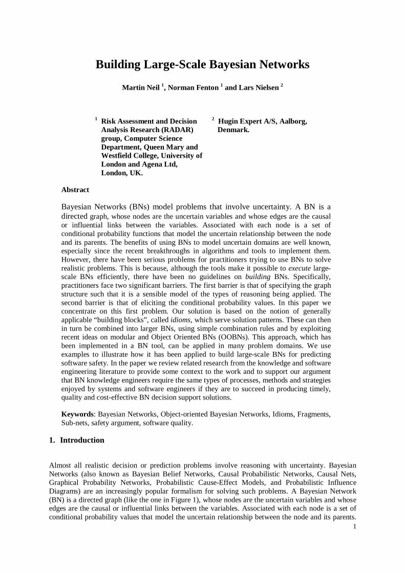
Almost all realistic decision or prediction problems involve reasoning with uncertainty. Bayesian Networks (also known as Bayesian Belief Networks, Causal Probabilistic Networks, Causal Nets, Graphical Probability Networks, Probabilistic Cause-Effect Models, and Probabilistic Influence Diagrams) are an increasingly popular formalism for solving such problems. A Bayesian Network (BN) is a directed graph (like the one in Figure 1), whose nodes are the uncertain variables and whose edges are the causal or influential links between the variables. Associated with each node is a set of conditional probability values that model the uncertain relationship between the node and its parents.

2

The underlying theory of BNs combines Bayesian probability theory and the notion of conditional independence. For introductory tutorial material on BNs see [Agena 1999, Hugin 1999].

Although Bayesian probability theory has been around for a long time it is only since the 1980s that efficient algorithms (and tools to implement them) taking advantage of conditional independence have been developed [Jensen 1996, Gilks et al 1994]. The recent explosion of interest in BNs is due to these developments, which mean that realistic size problems can now be solved. These recent developments, in our view, make BNs the best method for reasoning about uncertainty.

To date BNs have proven useful in applications such as medical diagnosis and diagnosis of mechanical failures. Their most celebrated recent use has been by Microsoft where BNs are used in the intelligent help assistants in Microsoft Office [Heckerman and Horvitz 1998]. Our own interest in applying BNs stems from the problem of predicting reliability of complex systems. Our objective was to improve predictions about these systems by incorporating diverse evidence, such as subjective judgements about the quality of the design process, along with objective data such as the test results themselves. Since 1993 we have been involved in many collaborative R&D projects in which we have built BNs for real applications ranging from predicting vehicle reliability for the UK Defence Research Agency to predicting software quality in consumer electronics [SERENE 1999a, Fenton et al 1999].

system safety

faults found intesting

testing accuracy

quality of testteam

solutioncomplexity

operationalusage

correctness ofsolution

supplier qualityintrinsic

complexity

Figure 1: Example Bayesian Network

Because of our extensive practical use of BNs we are well aware of their benefits in modelling uncertain domains. However, we are also aware of the problems. Practitioners wishing to use BNs to solve large-scale problems have faced two significant barriers that have dramatically restricted exploitation. The first barrier is that of producing the ‘right’ graph — one that it is a sensible model of the types of reasoning being applied. The second barrier occurs when eliciting the conditional probability values, from a domain expert. For a graph containing many combinations of nodes, where each may have a large number of discrete or continuous values, this is infeasible. Although there has been extensive theoretical research on BN’s there is little guidance in the literature on how to tackle these two problems of scale. In the SERENE project [SERENE 1999a] we arrived at what we feel are very good partial solutions to both problems, but in this paper we concentrate on the first problem of specifying a sensible BN graph structure. Although crucial to the implementation of BNs we do not need to make any assumptions about probability assignments to support the arguments made in this

3

paper. A detailed description of how we have addressed the probability elicitation problem is the subject of a separate paper.

The SERENE project involved several partners (CSR, Hugin, ERA Technology, Electricite de France, Tüv Hamburg and Objectif Technologie) all building BNs to model different safety assessment approaches. CSR (City University) and Hugin were the technology providers. At the same time a consultancy company, Agena Ltd, was set-up by CSR personnel to apply BNs in other real-world projects. Recently we have set-up the Risk Assessment and Decision Analysis Research (RADAR) group at Queen Mary and Westfield College, University of London, to pursue our research ideas. As a result of an analysis of many dozens of BNs we discovered that there were a small number of generally applicable “building blocks” from which all the BNs could be constructed. These building blocks, which we call “idioms”, can be combined together into objects. These can then in turn be combined into larger BNs, using simple combination rules and by exploiting recent ideas on Object Oriented BNs (OOBNs). The SERENE tool [SERENE 1999b] and method [SERENE 1999a] was constructed to implement these ideas in the domain of system safety assessment. However, we believe these ideas can be applied in many different problem domains. We believe our work is a major breakthrough for BN applications.

From a practitioner’s point of view the process of compiling and executing a BN, using the latest software tools, is relatively painless given the accuracy and speed of the current algorithms. However, the problems of building a complete BN for a particular ‘large’ problem remain i.e. how to:

• Build the graph structure;

• Define the node probability tables for each node of the graph.

Despite the critical importance the graph plays there is little guidance in the literature on how to build an appropriate graph structure for a BN. Where realistic examples have been presented in the literature they have been presented as a final result without any accompanying description of how they arrived at the particular graph. In the literature much more attention is given to the algorithmic properties of BNs rather than the method of actually building them in practice.

In Section 2 we provide an overview of the foundations of BNs and in Section 3 we review related work from the software and knowledge engineering literature on how to build BN models in practice. This provides some motivation for our ideas on the BN development process, the implementation of OOBNs in the SERENE tool and the use of idioms to enable pattern matching and reuse. These are discussed in Section 4 on building large scale BNs. The idioms are defined and described in Section 5, and some example idiom instantiations are provided for each idiom. Section 6 gives an example of how a real BN application, for system safety assessment, was constructed using idioms and objects. In Section 7 we offer some conclusions, and describe briefly our complementary work to solve the second problem of building large-scale BNs, namely defining large probability tables.

2. Bayesian networks

BNs enable reasoning under uncertainty and combine the advantages of an intuitive visual representation with a sound mathematical basis in Bayesian probability. With BNs, it is possible to articulate expert beliefs about the dependencies between different variables and to propagate consistently the impact of evidence on the probabilities of uncertain outcomes. BNs allow an injection of scientific rigour when the probability distributions associated with individual nodes are simply ‘expert opinions’.

A Bayesian network (BN) is a causal graph where the nodes represent random variables associated with a node probability table (NPT).

4

The causal graph is a directed graph where the connections between nodes are all directed edges (see Figure 1). The directed edges define causal relationships1. If there is a directed edge (link) from node A to node B, A might be said to have causal impact on B.

For example, in Figure 1 poor quality suppliers are known to accidentally introduce faults in software products (incorrectness) so in this BN there would be a link from node “supplier quality” to node “correctness of solution”. We shall talk about parents and children when referring to links. We say that an edge goes from the parent to the child.

The nodes in the BN represent random variables. A random variable has a number of states (e.g. “yes” and “no”) and a probability distribution for the states where the sum of the probabilities of all states should be 1. In this way a BN model is subject to the standard axioms of probability theory.

The conditional probability tables associated with the nodes of a BN determine the strength of the links of the graph and are used to calculate the probability distribution of each node in the BN. Specifying the conditional probability of the node given all its parents (the parent nodes having directed links to the child node) does this. In our example the node “correctness of solution” had “intrinsic complexity” and “supplier quality” as parents, the conditional probability table p(correctness of solution | supplier quality, intrinsic complexity) should be associated with node “correctness of solution”. If a node has no parents a prior probability table of this node is associated with it. This is simply a distribution function of the states of the node.

In order to reduce the number of possible combinations of node relations in the model BNs are constructed using assumptions about the conditional dependencies between nodes. In this way we can reduce the number of node combinations that we have to consider. For example, in our model, from Figure 1, the number of valid connections between nodes has been reduced, by virtue of the conditional dependence assumptions, from nine factorial to ten. Nodes that are directly dependent, either logically or by cause-effect, are linked in the graph. Nodes that are indirectly dependent on one another, but which are not directly linked, are connected through a chain of shared linked nodes. Therefore, by using domain knowledge we can produce a model that makes sense and reduces the computational power needed to solve it.

Once a BN is built it can be executed using an appropriate propagation algorithm, such as the Hugin algorithm [Jensen 1996]. This involves calculating the joint probability table for the model (probability of all combined states for all nodes) by exploiting the BN’s conditional probability structure to reduce the computational space. Even then, for large BNs that contain undirected cycles the computing power needed to calculate the joint probability table directly from the conditional probability tables is enormous. Instead, the junction tree representation is used to localise computations to those nodes in the graph that are directly related. The full BN graph is transformed into the junction tree by collapsing connected nodes into cliques and eliminating cyclic links between cliques. The key point here is that propagating the effects of observations throughout the BN can be done using only messages passed between – and local computations done within – the cliques of the junction tree rather than the full graph. The graph transformation process is computationally hard but it only needs to be produced once off-line. Propagation of the effects of new evidence in the BN is performed using Bayes’ theorem over the compiled junction tree. For full details see [Jensen 1996].

Once a BN has been compiled it can be executed and exhibits the following two key features:

1 Strictly speaking a BN is a mathematical formalism where the directed edges model conditional dependency relations. Such a definition is free from semantic connotations about the real world. However, what makes BNs so powerful as a method for knowledge representation, is that the links can often be interpreted as representations of causal knowledge about the world. This has the advantage of making BNs easier to understand and explain. Clearly, given the broad definition of conditioning, BNs can also model deterministic, statistical and analogical knowledge in a meaningful way.

5

• The effects of observations entered into one or more nodes can be propagated throughout the net, in any direction, and the marginal distributions of all nodes updated;

• Only relevant inferences can be made in the BN. The BN uses the conditional dependency structure and the current knowledge base to determine which inferences are valid.

3. Related work

In this section we begin with a brief overview of the textbook literature on building the digraph component of a BN (Section 3.1). Next, in Section 3.2, we examine the role of modules and object orientation in representing and organising a BN. Recent work on building BNs from fragments is described in Section 3.3 and finally we discuss ways of managing the process of BN construction in Section 3.4. In reviewing related work we focused on research done specifically on knowledge engineering of large BNs but also put such research in the wider systems and software engineering context because we believe that knowledge and software engineers share the same problems and challenges.

We do not review all of the tricks and tips that might help the practitioner build BNs in practice, like noisy-OR [Jensen 1996] or the partitioning of probability tables [Heckerman 1990]. As we mentioned earlier we avoid discussing the difficult problem of how to build probability tables in this paper, not because we don’t have anything to say here, but because getting the digraph structure right is a pre-requisite for meaningful elicitation of any probabilities. Probability elicitation for very large BNs can be done. The Hailfinder project [Hailfinder 1999] presents a very positive experience of probability elicitation free of the problems presented in the cognitive psychology literature [Wright and Ayton 1994].

3.1 Building the BN digraph

Much of the literature on BNs uses very simple examples to show how to build sensible digraphs for particular problems. The standard texts on BNs, Pearl [Pearl 1988] and Jensen [Jensen 1996], use examples where Mr. Holmes and Dr. Watson are involved in a series of episodes where they wish to infer the probability of icy roads, burglary and earthquakes from uncertain evidence. The earthquake example is as follows:

Mr Holmes is working at his office when he received a telephone call from Watson who tells him that Holmes’ burglar alarm has gone off. Convinced that a burglar has broken into his house, Holmes rushes into his car and heads for home. On his way he listens to the radio, and in the news it is reported that there has been a small earthquake in the area. Knowing that the earthquake has a tendency to turn the burglar alarm on, he returns to his work leaving his neighbours the pleasure of the noise. (from Jensen 1996)

6

burglary

alarm sounds

earthquake

radio report

Figure 2: A BN model for the earthquake example

Figure 2 shows the BN for this example. The nodes here are all Boolean — their states are either true or false. There are two key points to note here:

1. The example is small enough that the causal directions of the edges are obvious. A burglary causes the alarm to sound; the earthquake causes the radio station to issue a news report and also causes the alarm to sound.

2. The actual inferences made can run counter to the edge directions. From the alarm sounding Holmes inferred that a burglary had taken place and from the radio sounding he inferred that an earthquake had occurred. Only when explaining away the burglary hypothesis did Holmes reason along the edge from earthquake to alarm.

Real-life problems are rarely as small as this example — how then do we scale-up what we can learn from small, often fictitious examples, to real world prediction problems? Also, given that we could build a large BN for a real problem we need to ensure that the edge directions represented do not conflate “cause to effect" node directions with the node directions implied by the inferences we might wish to make. Figure 3 shows a simple example of this where we model the act of placing a hand through and open window to assess the temperature.

temperatureoutside

cold hand

cold hand

temperatureoutside

(a) (b)

Figure 3: Edge direction problem

In Figure 3 (a), the two nodes “temperature outside” and “cold hand” have the following conditional probability tables:

p(temperature outside), p(cold hand | temperature outside)

In Figure 3 (b), the conditional probability tables are:

7

p(temperature outside | cold hand), P(cold hand)

Mathematically there is no reason to choose one over the other in this small case you can in both cases calculate the marginal distribution for each of them correctly. However in practical situations mathematical equivalence is not the sole criterion. Here the causal relationship is modelled by (a) because the temperature outside causes one’s hand to become cold. It is also easier to think of what the prior probability distribution for the temperature outside rather than think of the prior distribution of having cold hands independent of the outside temperature.

From the perspective of probability elicitation it seems easier, though, to consider

p(temperature outside | cold hands)

rather than

p(cold hands | temperature outside)

simply because the arrow follows the direction of the inference we wish to make; we reason from the evidence available to the claim made. A BN can model both of these successfully in the sense that “cause to effect” and “effect to cause” are mathematically equivalent. However, applying uniform interpretations are critical if we are to build large networks with meaningful semantics.

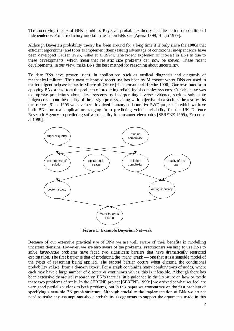
In BNs the process of determining what evidence will update which node is determined by the conditional dependency structure. The main area of guidance for building sensible structures stem from the definitions of the three types of dependency connection or “d-connection”.

In a BN three types of d-connection (dependency) topology, and how they operate, have been identified and are shown in Figure 4.

A B C

A B C

A B C

(a) - pipeline

(b) - converging

(c) - diverging

Figure 4: Pipeline, converging and diverging d-connections

The definitions of the different types of d-connection are:

8

a) Serial d-connection: Node C is conditionally dependent and B is conditionally dependent on A. Entering hard evidence at node A or C will lead to an update in the probability distribution of B. However, if we enter evidence at node B only we say that nodes A and C are conditionally independent given evidence at node B. This means that evidence at node B “blocks the pipeline”.

b) Converging d-connection: Node B is conditionally dependent on nodes A and C. Entering hard evidence at node A will update node B but will have no effect on node C. If we have entered evidence at node B then entering evidence at node A will update node C. Here nodes A and C are conditionally dependent given evidence at node B.

c) Diverging d-connection: Node A and C are conditionally dependent on node B. Entering hard evidence at node B will effect nodes A and C, but if we then enter evidence on node A it will not effect C when there is evidence at node B. Here nodes A and C are conditionally independent given evidence at node B.

By using these ideas we can postulate topologies connecting small numbers of nodes and hypothesise the effects of entering evidence at one node on another. The answer to the question “would entering data here effect the conclusion reached here, given that we know this datum over here?” might help indicate the type of d-connection at play in the expert’s reasoning. Clearly this process is very difficult to apply in practice because experts do not easily think in terms of conditional dependencies and it can only be done reasonably for small BN topologies.

3.2 Modules and Object-Orientation

The benefits of constructing software systems from components or modules are well known and the properties that modular systems must contain were articulated as early as 1972 [Parnas, 1972]. In the 1970s and early 1980s structured methods were introduced, such as Jackson-structured Design (JSD) method [Jackson 1975], to help control complexity and the intellectual process of large-systems design. Crucial concepts in the structured approach included functional decomposition and abstract data types.

In the late 1980s object-oriented (OO) methods were introduced as a way of maximising reuse of modules by ensuring that modules were well formed and their interface complexity was controlled [Booch 1993], [Rumbaugh et al 1991]. OO methods are now in widespread use, the most prominent being the Unified Modelling Language (UML) [Booch et al 1998]. OO design methods exhibit a number of desirable properties, the major ones being abstraction, inheritance and encapsulation. Abstraction allows the construction of classes of objects that are potentially more reusable and internally cohesive. Inheritance via a hierarchical organisation means that objects can inherit attributes and computational operations of parent classes. Encapsulation ensures that the methods and attributes naturally belonging to objects are self-contained and can only be accessed via their public interfaces.

In [Koller and Pfeffer, 97] an OO approach has been adopted for representing and constructing large BNs (the approach is naturally called OOBNs). Network fragments become classes, both variables (nodes) and instantiated BN fragments become objects (simple and complex) and encapsulation is implemented via interface and private variables. However, they stopped short of defining a fully OO method of inheritance via a class hierarchy and did not cover any of the more esoteric features of OO like dynamic polymorphism.

The key benefits of OOBNs to the practitioner are that both knowledge declaration and probabilistic inference are modular. Individual objects should be separately compilable and query complete. Also the OO representation specifies an organised structure for elicitation of the graph structure and navigation during use.

9

3.3 Building BNs from fragments

It is standard practice in systems and software engineering to build systems from the “bottom-up” using components or modules that when joined together, perhaps using OO methods, form the complete system [Sommerville 1992]. The bottom-up approach relies matching problems to solutions in the form of reusable programs or designs. In contrast, historically the BN literature has presented “complete”, albeit small, BNs in their entirety without describing how the complete BN came to be.

Laskey and Mahoney recognised that BN construction required a method for specifying knowledge in larger, semantically meaningful, units they called network “fragments” [Laskey and Mahoney 1997]. Before their work it was not clear explicitly how BNs might best be organised as components or modules. Laskey and Mahoney also argued that current approaches lacked a means of constructing BNs from components and ways of varying BN models from problem instance to problem instance.

Under their scheme a fragment is a set of related random variables that could be constructed and reasoned about separately from other fragments. Ideally fragments must make sense to the expert who must be able to supply some underlying motive or reason for them belonging together. Additionally fragments should formally respect the syntax and semantics of BNs. Also, in [Mahoney and Laskey 1996] they demonstrate the use of stubs to represent collections of BN nodes that have yet to be defined with the purpose of allowing early prototyping of partial BNs.

Laskey and Mahoney use OO concepts to represent and manipulate fragments. Input and resident variables are used to specify interfaces and encapsulate private data respectively. Two types of object were identified input and result fragments. Input fragments are composed together to form a result fragment. To join input fragments together an influence combination rule is needed to compute local probability distributions for the combined, or result, fragment. For example a fragment p(A | B) might be joined to p(A | C) to yield the result fragment p(A | B, C) using an influence combination rule, such as noisy-OR, to define the NPT for p(A | B, C).

Encapsulation is central to Koller and Pfeffer’s definition of an OOBN. Encapsulated objects or modules should be loosely connected and cohesive [Myers 1975]. However, despite their purported adoption of OO ideas Laskey and Mahoney scheme does not strictly adhere to this requirement. This is because different fragments can contain the same child node as a resident variable and, as a consequence of this, when creating a fragment we must know whether it shares resident nodes with other fragments in order to define the influence combination rule. Clearly this is not a problem when the influence combination rule treats all parent nodes equally irrespective of type and value, as a form of dynamic polymorphism, but such a combination rule would be difficult to conceive and implement.

3.4 Managing systems development

Large knowledge based systems, including BNs, are subject to the same forces as any other substantial engineering undertaking. The customer might not know what they want; the knowledge engineer may have difficulty understanding the domain; the tools and methods applied may be imperfect; dealing with multiple ever-changing design abstractions is difficult etc. In the end these issues, along with people, economic and organisational factors will impact on the budget, schedule and quality of the end product.

Explicit management is necessary for large BN projects. Knowledge engineers need to manage the representation and construction of BNs using methods like OOBNs and fragments. They also need processes for specifying, designing, implementing, evaluating and changing the BN system and its intermediate representations. In software engineering the choice of process centres around the management of risk [Boehm 1981]. Risky projects can be characterised by ill-understood and ambiguous requirements, inexperienced solution providers and complex technology. Incremental development, prototyping and time-boxing are recommended processes for such risky projects

10

because they attempt to resolve requirements problems early and provide some means of evaluating the solution as it progresses. The key to success here is the existence of feedback loops within the process, such as those present in the spiral model [Boehm 1981]. For more established problem domains, with fewer risks, a sequential life-cycle process is adequate. This simply involves specifying, designing, implementing and testing the solution in one sequence with few or no feedback steps. Of course, both processes are simplified extremes and most projects will experience a mixture of both in practice.

The problem of managing different levels of BN refinement and the need for a systems engineering process have been recognised [Mahoney and Laskey 1996]. Knowledge engineering is a process of discovery over time, not extraction of a perfect problem statement from an expert that can be automatically turned into a BN solution in a single step. Knowledge engineers work with the expert to decompose the system, recognise patterns at the macro and micro level [Shaw and Garland 1996] and continually change the model as the understanding of both sides’ increases.

4. Building large-scale BNs

Our approach to dealing with the problems of building large-scale BNs has been influenced by the experiences and innovations described in Section 3. We identified three main goals to improve how we build any large BN system:

1. Apply a process that explicitly manages the risks presented during development;

2. Apply a means of combining components together in such a way that complexity is easily managed;

3. Develop a means of easily identifying and constructing small, reusable, components that form the foundations of a BN.

4.1 Process model

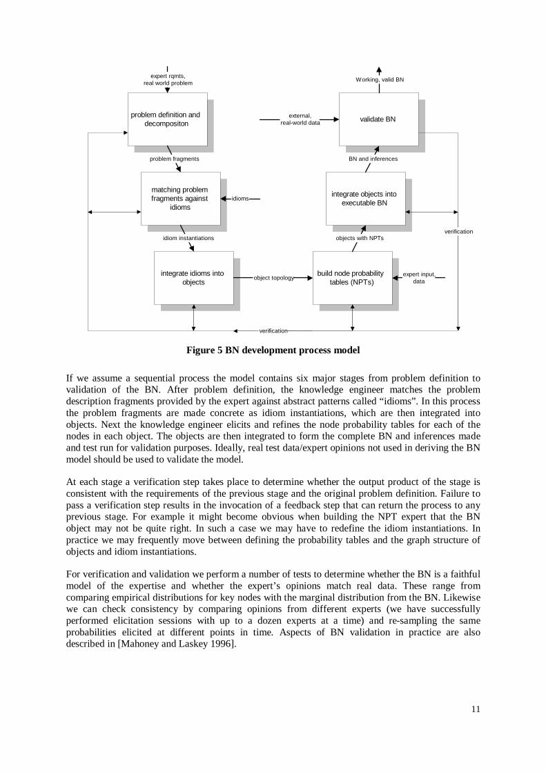
With regard to our first goal — applying a process that manages risk — we developed a derivative of the spiral model tailored for BN development. This is shown in Figure 5 where boxes represent the processes and the process inputs/outputs are shown by directed arcs labelled with the input/output names. Note that only the major stages and artefacts are shown. Note that we are describing a very simple model of BN construction. In practice the BNs we develop are embedded in larger software-based decision-support systems. Therefore in practice the BN development process is a sub-process of a larger software engineering process.

11

problem definition anddecompositon

matching problemfragments against

idioms

integrate idioms intoobjects

build node probabilitytables (NPTs)

integrate objects intoexecutable BN

validate BN

problem fragments

idiom instantiations

object topology

objects with NPTs

BN and inferences

Working, valid BNexpert rqmts,

real world problem

idioms

expert input,data

external,real-world data

verification

verification

Figure 5 BN development process model

If we assume a sequential process the model contains six major stages from problem definition to validation of the BN. After problem definition, the knowledge engineer matches the problem description fragments provided by the expert against abstract patterns called “idioms”. In this process the problem fragments are made concrete as idiom instantiations, which are then integrated into objects. Next the knowledge engineer elicits and refines the node probability tables for each of the nodes in each object. The objects are then integrated to form the complete BN and inferences made and test run for validation purposes. Ideally, real test data/expert opinions not used in deriving the BN model should be used to validate the model.

At each stage a verification step takes place to determine whether the output product of the stage is consistent with the requirements of the previous stage and the original problem definition. Failure to pass a verification step results in the invocation of a feedback step that can return the process to any previous stage. For example it might become obvious when building the NPT expert that the BN object may not be quite right. In such a case we may have to redefine the idiom instantiations. In practice we may frequently move between defining the probability tables and the graph structure of objects and idiom instantiations.

For verification and validation we perform a number of tests to determine whether the BN is a faithful model of the expertise and whether the expert’s opinions match real data. These range from comparing empirical distributions for key nodes with the marginal distribution from the BN. Likewise we can check consistency by comparing opinions from different experts (we have successfully performed elicitation sessions with up to a dozen experts at a time) and re-sampling the same probabilities elicited at different points in time. Aspects of BN validation in practice are also described in [Mahoney and Laskey 1996].

12

4.2 OOBNs using the SERENE tool

In the SERENE project a prototype software tool was developed to allow practitioners in the area of safety assessment to build modular BNs from idiom instances. The basic look and feel was based on the Hugin tool [Hugin 1999], and an OOBN approach based on the [Koller and Pfeffer, 97] framework.

The tool allows the construction of BN objects with a subset of its nodes defined to be interface nodes. The purpose of the interface nodes is to join one object instantiation with other object instantiations (object instantiations are called abstract nodes). Interface variables are divided into input and output nodes where input variables are place holders for external nodes and output nodes are visible internal nodes that can be used as parents of external nodes or as join links to input nodes.

Figure 6 demonstrates how it would be possible in the SERENE tool to create two objects (left) and then afterwards instantiate them and combine them inside a third object (right). The dashed, shaded, nodes represent input nodes while the thick lined, shaded, nodes represent output nodes. Nodes a, b and c in Object1 are input nodes. Nodes d, e and f in Object1 are output nodes.

Abstract nodes are displayed with input nodes at the top and output nodes at the bottom. We use dot (.) notation when we refer to the interface nodes of abstract nodes. For example, Abstract1.c is the lower left interface variable of object Abstract1.

a b

Private2

e

c

Private3 d

Private1

Object1

Object2

f g

h Private1

a b

e c d

Abstract1

f g

h

External2

Abstract2

External1

Object3

Figure 6: Two ‘leaf’ templates, Object1 and Object2, instantiated into abstract nodes, Abstract1 and Abstract2 (respectively), inside Object3 and then combined through their interface

variables

Looking at Object3 you will notice two different kinds of arcs. There are ordinary causal arcs from Abstract1.c and Abstract1.d to node External2. Then, there are two double line arcs from External1 to Abstract1.a and Abstract1.e to Abstract2.f. These are join links stating that the child node is a placeholder for the parent node inside the abstract node. Nodes joined together must be of the same type (discrete numeric, interval, discrete labelled, Boolean) and have same labels or intervals. For example the if the node Object1.e is a discrete numeric node with labels {0,1,2,3} then the node Object2.f must also be discrete numeric with the same labels.

13

4.3 Identifying reusable patterns as idioms

OOBNs, the use of BN fragments and a process for BN construction together only solve part of the systems engineering problem. We are still left with the challenge of actually identifying the components we might wish to combine together into BN objects. When building software objects programmers and designers recognise commonly occurring problem types or patterns that serve to guide the solution to that particular problem [Jackson 1995].

From our experience of building BNs in a range of application domains we found that experts were applying very similar types of reasoning, over subtly different prediction problems. Moreover, they often experienced the same kind of difficulties in trying to represent their ideas in the BN model. In summary these problems were in deciding:

• Which edge direction to choose;

• Whether some of the statements they wished to make were actually uncertain and if not whether they could be represented in a BN;

• What level of granularity was needed when identifying nodes in the BN;

• Whether competing models could somehow be reconciled into one BN model at all.

As a result of these experiences and the problems encountered when trying to build reasonable graph models we identified a small number of natural and reusable patterns in reasoning to help when building BNs. We call these patterns “idioms”. An idiom is defined in the Webster’s Dictionary (1913) as:

“The syntactical or structural form peculiar to any language; the genius or cast of a language.”

We use the term idiom to refer to specific BN fragments that represent very generic types of uncertain reasoning. For idioms we are interested only in the graphical structure and not in any underlying probabilities. For this reason an idiom is not a BN as such but simply the graphical part of one. We have found that using idioms speeds up the BN development process and leads to better quality BNs.

Although we believe we are the first to develop these ideas to the point where they have been exploited, the ideas are certainly not new. For example, as early as 1986 Judea Pearl recognised the importance of idioms and modularity when he remarked:

“Fragmented structures of causal organisations are constantly being assembled on the fly, as needed, from a stock of building blocks” [Pearl 1986]

The use of idioms fills a crucial gap in the literature on engineering BN systems by helping to identify the semantics and graph structure syntax of common modes of uncertain reasoning. Also, the chances of successful elicitation of probability values for NPTs from experts is greatly improved if the semantics of the idiom instantiation is well understood.

We can use idioms to reuse existing solution patterns, join idiom instantiations to create objects and with OOBNs combine objects to make systems. In every day use we have found that the knowledge engineer tends to view and apply idioms much like structured programming constructs such as IF-

14

THEN-ELSE and DO-WHILE statements [Dijkstra 1976]. We believe the same benefits accrue when when “structured” and standard idioms are employed like structured programming constructs [Dijkstra 1968].

In our view fragments, as defined by Laskey and Mahoney, constitute smaller BN building blocks than idiom instantiations. Syntactically an idiom instantiation is a combination of fragments. However, we would argue that an idiom instance is a more cohesive entity than a fragment because the idiom from which it is derived has associated semantics. A fragment can be nothing more than a loose association of random variables that are meaningful to the expert, but the semantics of the associations within a fragment need to be defined anew each time a fragment is created. Thus, the use of fragments only does not lead to reuse at the level of reasoning, only at a domain specific level.

5. Idioms

The five idioms identified are:

• Definitional/Synthesis idiom — models the synthesis or combination of many nodes into one node for the purpose of organising the BN. Also models the deterministic or uncertain definitions between variables;

• Cause-consequence idiom — models the uncertainty of an uncertain causal process with observable consequences;

• Measurement idiom — models the uncertainty about the accuracy of a measurement instrument;

• Induction idiom — models the uncertainty related to inductive reasoning based on populations of similar or exchangeable members;

• Reconciliation idiom — models the reconciliation of results from competing measurement or prediction systems.

We claim that for constructing large BNs domain knowledge engineers find it easier to use idioms to construct their BN than following textbook examples or by explicitly examining different possible d-connection structures between nodes, under different evidence scenarios. This is because the d-connection properties required for particular types of reasoning are preserved by the idioms and emerge through their use. Also, because each idiom is suited to model particular types of reasoning, it is easier to compartmentalise the BN construction process.

In the remainder of this section we define these idioms in detail. Idioms act as a library of patterns for the BN development process. Knowledge engineers simply compare their current problem, as described by the expert, with the idioms and reuse the appropriate idiom for the job. By reusing the idioms we gain the advantage of being able to identify objects that should be more cohesive and self-contained than objects that have been created without some underlying method. Also the use of idioms encourages reuse.

Idiom instantiations are idioms made concrete for a particular problem, with meaningful labels, but again without defining the probability values. Once probability values have been assigned then they become equivalent to objects in an OOBN and can be used in an OOBN using the same operations as other objects. This is covered in Section 5.

We do not claim that the idioms identified here form an exhaustive list of all of the types of reasoning that can be applied in all domains. We have identified idioms from a single, but very large domain —

15

that of systems engineering. BN developers in this domain should find these idioms useful starting points for defining sensible objects, but, since we are not claiming completeness, may decide to identify and define new idioms. However, we do believe that these idioms can be applied in domains other than systems engineering and as such could provide useful short cuts in the BN development process.

5.1 The Definitional/Synthesis Idiom

Although BNs are used primarily to model causal relationships between variables, one of the most commonly occurring class of BN fragments is not causal at all. The definitional/synthesis idiom, shown in Figure 7, models this class of BN fragments and covers each of the following cases where the synthetic node is determined by the values of its parent nodes using some combination rule.

node 1

synthetic node

node 2 node n

Figure 7: Definitional/synthesis idiom

Case 1. Definitional relationship between variables. In this case the synthetic node is defined in terms of the nodes: node1, node2, …, node n (where n be can be any integer). This does not involve uncertain inference about one thing based on knowledge of another. For example, “velocity”, V, of a moving object is defined in terms of “distance” travelled, D, and “time”, T, by the relationship, V = D/T.

distance

velocity

time

Figure 8: Instantiation of definitional/synthesis idiom for velocity example

Although D and T alone could be represented in a BN (and would give us all of the information we might need about V), it is useful to represent V in the BN along with D and T (as shown in Figure 8). For example, we might be interested in other nodes conditioned on V.

Clearly synthetic nodes, representing definitional relations, could be specified as deterministic functions where we are certain of the relationship between the concepts. Otherwise we would need to use probabilistic functions to state the degree to which some combination of parent nodes combine to define some child node. Such a probabilistic relationship would be akin to a principal components

16

model where some unobservable complex attribute is defined as a linear combination of random variables [Dillan and Goldstein 1984].

One of the first issues we face when building BNs is whether we can combine variables using some hierarchical structure using a valid organising principle. We might view some nodes as being of the same type or having the same sort and degree of influence on some other node and might then wish to combine these. A hierarchy of concepts is simply modelled as a number of synthesis/definitional idioms joined together.

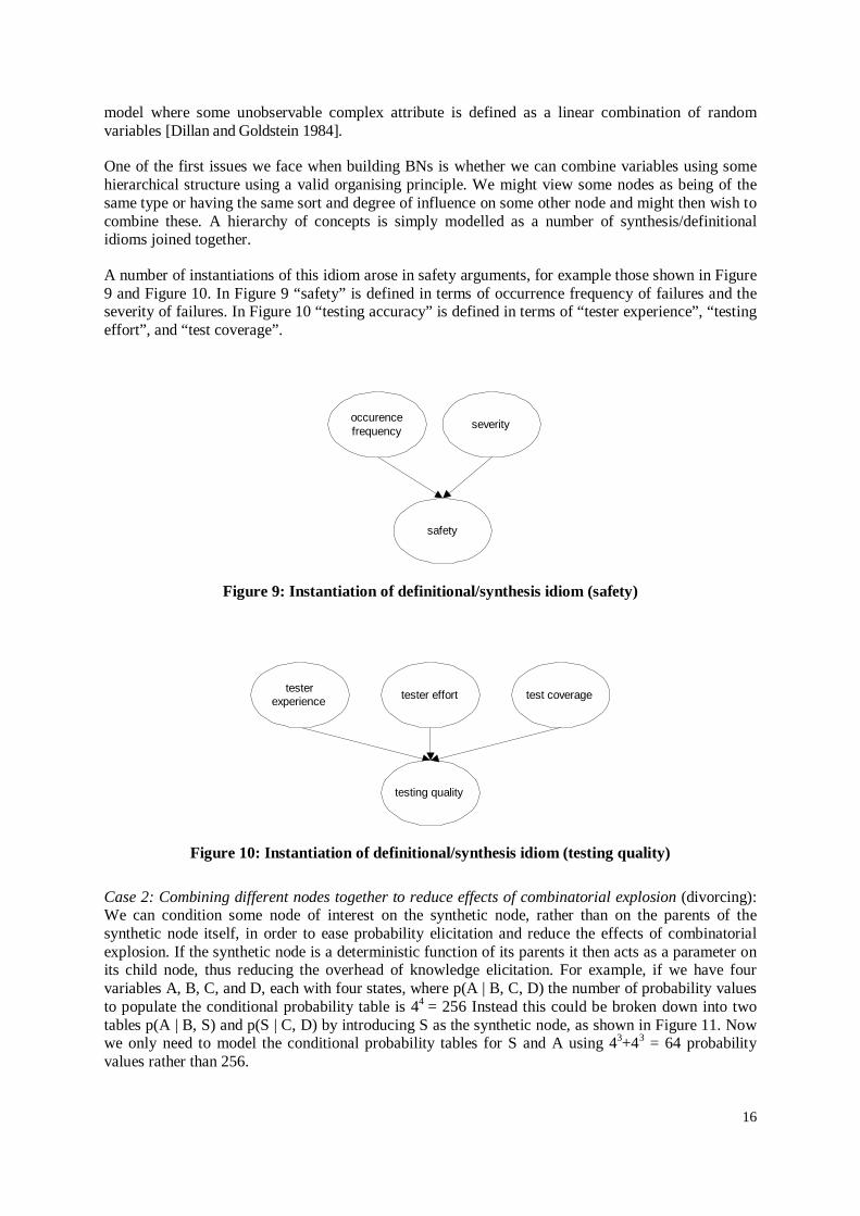
A number of instantiations of this idiom arose in safety arguments, for example those shown in Figure 9 and Figure 10. In Figure 9 “safety” is defined in terms of occurrence frequency of failures and the severity of failures. In Figure 10 “testing accuracy” is defined in terms of “tester experience”, “testing effort”, and “test coverage”.

occurencefrequency

safety

severity

Figure 9: Instantiation of definitional/synthesis idiom (safety)

testerexperience

testing quality

tester effort test coverage

Figure 10: Instantiation of definitional/synthesis idiom (testing quality)

Case 2: Combining different nodes together to reduce effects of combinatorial explosion (divorcing): We can condition some node of interest on the synthetic node, rather than on the parents of the synthetic node itself, in order to ease probability elicitation and reduce the effects of combinatorial explosion. If the synthetic node is a deterministic function of its parents it then acts as a parameter on its child node, thus reducing the overhead of knowledge elicitation. For example, if we have four variables A, B, C, and D, each with four states, where p(A | B, C, D) the number of probability values to populate the conditional probability table is 44 = 256 Instead this could be broken down into two tables p(A | B, S) and p(S | C, D) by introducing S as the synthetic node, as shown in Figure 11. Now we only need to model the conditional probability tables for S and A using 43+43 = 64 probability values rather than 256.

17

This technique of cutting down the combinatorial space using synthetic nodes has been called divorcing by [Jensen 1996]. Here the synthetic node, S, divorces the parents C and D from B.

B

A

C D

S

Figure 11: Divorcing of a definitional/synthesis idiom instantiation.(The dotted links are the “old” links and the bold links and node are new.)

Parent nodes can only be divorced from one another when their effects on the child node can be considered separately from the other non-divorced parent node(s). For a synthetic node to be valid some of its parent node state combinations must be exchangeable, and therefore equivalent, in terms of their effect on the child node. These exchangeable state combinations must also be independent of any non-divorcing parents, again in terms of their effects on the child node. In Figure 11 nodes C and D are assumed exchangeable with respect to their effects on A. So, for a given change in the state value of S it does not matter whether this was caused by a change in either C or D when we come to consider p(A | B, S). Also, when considering the joint effect of parent nodes B and S on child node A it does not matter whether the state values of node S have been determined by either node C or node D.

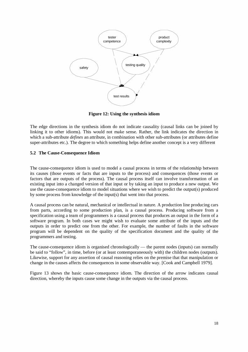
To illustrate this we can consider an example with the topology shown in Figure 11 where node A is “test results” gained from a campaign of testing, B is the “safety” of the system and C and D represent “tester competence” and “product complexity” respectively. We can create a synthetic node S “testing quality” to model the joint effects of “tester competence” and “product complexity” on the “test results”. This new BN is shown in Figure 12. Implicit in this model is the assumption that tester competence and product complexity operate together to define some synthetic notion of testing quality where, when it comes to eliciting values for p(test results | safety, testing quality), it does not matter whether poor quality testing has been caused by incompetent testers or a very complex product.

18

safety

test results

testercompetence

productcomplexity

testing quality

Figure 12: Using the synthesis idiom

The edge directions in the synthesis idiom do not indicate causality (causal links can be joined by linking it to other idioms). This would not make sense. Rather, the link indicates the direction in which a sub-attribute defines an attribute, in combination with other sub-attributes (or attributes define super-attributes etc.). The degree to which something helps define another concept is a very different

5.2 The Cause-Consequence Idiom

The cause-consequence idiom is used to model a causal process in terms of the relationship between its causes (those events or facts that are inputs to the process) and consequences (those events or factors that are outputs of the process). The causal process itself can involve transformation of an existing input into a changed version of that input or by taking an input to produce a new output. We use the cause-consequence idiom to model situations where we wish to predict the output(s) produced by some process from knowledge of the input(s) that went into that process.

A causal process can be natural, mechanical or intellectual in nature. A production line producing cars from parts, according to some production plan, is a causal process. Producing software from a specification using a team of programmers is a causal process that produces an output in the form of a software program. In both cases we might wish to evaluate some attribute of the inputs and the outputs in order to predict one from the other. For example, the number of faults in the software program will be dependent on the quality of the specification document and the quality of the programmers and testing.

The cause-consequence idiom is organised chronologically — the parent nodes (inputs) can normally be said to “follow”, in time, before (or at least contemporaneously with) the children nodes (outputs). Likewise, support for any assertion of causal reasoning relies on the premise that that manipulation or change in the causes affects the consequences in some observable way. [Cook and Campbell 1979].

Figure 13 shows the basic cause-consequence idiom. The direction of the arrow indicates causal direction, whereby the inputs cause some change in the outputs via the causal process.

19

input

output

Figure 13: The Cause-consequence Idiom

The underlying causal process is not represented, as a node, in the BN in Figure 13. It is not necessary to do so since the role of the underlying causal process, in the BN model, is represented by the conditional probability table connecting the output to the input. This information tells us everything we need to know (at least probabilistically) about the uncertain relationship between causes and consequences.

Clearly Figure 13 offers a rather simplistic model of cause and effect since most (at least interesting) phenomena will involve many contributory causes and many effects. Joining a number of cause-consequence idioms together can create more realistic models, where the idiom instantiations have a shared output or input node. Also, to help organise the resulting BN one might deploy the synthesis idiom to structure the inputs or outputs.

A simple instantiation of two cause-consequence idioms, joined by the common node “failures”, is shown in Figure 14. Here we are predicting the frequency of software failures based on knowledge about “problem difficulty” and “supplier quality”.

problem difficulty

failures

supplier qulaity

Figure 14: Two cause-consequence idiom instantiations joined (software failures)

Here the process involves a software supplier producing a product. A good quality supplier will be more likely to produce a failure-free piece of software than a poor quality supplier. However the more difficult the problem to be solved the more likely is that faults may be introduced and the software fail.

5.3 Measurement Idiom

We can use BNs to reason about the uncertainty we may have about our own judgements, those of others or the accuracy of the instruments we use to make measurements. The measurement idiom represents uncertainties we have about the process of observation. By observation we mean the act of determining the true attribute, state or characteristic of some entity. The difference between this idiom and the cause-consequence idiom is that here one node is an estimate of the other rather then representing attributes of two different entities.

20

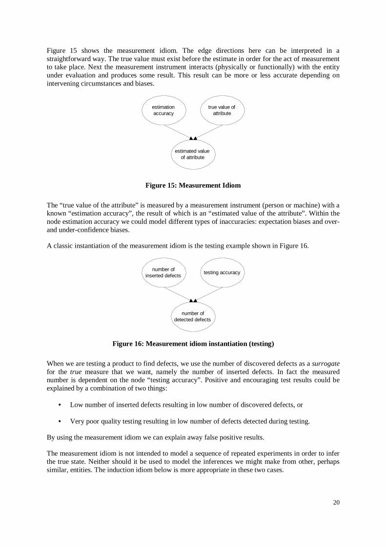
Figure 15 shows the measurement idiom. The edge directions here can be interpreted in a straightforward way. The true value must exist before the estimate in order for the act of measurement to take place. Next the measurement instrument interacts (physically or functionally) with the entity under evaluation and produces some result. This result can be more or less accurate depending on intervening circumstances and biases.

estimationaccuracy

estimated valueof attribute

true value ofattribute

Figure 15: Measurement Idiom

The “true value of the attribute” is measured by a measurement instrument (person or machine) with a known “estimation accuracy”, the result of which is an “estimated value of the attribute”. Within the node estimation accuracy we could model different types of inaccuracies: expectation biases and over- and under-confidence biases.

A classic instantiation of the measurement idiom is the testing example shown in Figure 16.

number ofinserted defects

number ofdetected defects

testing accuracy

Figure 16: Measurement idiom instantiation (testing)

When we are testing a product to find defects, we use the number of discovered defects as a surrogate for the true measure that we want, namely the number of inserted defects. In fact the measured number is dependent on the node “testing accuracy”. Positive and encouraging test results could be explained by a combination of two things:

• Low number of inserted defects resulting in low number of discovered defects, or

• Very poor quality testing resulting in low number of defects detected during testing.

By using the measurement idiom we can explain away false positive results.

The measurement idiom is not intended to model a sequence of repeated experiments in order to infer the true state. Neither should it be used to model the inferences we might make from other, perhaps similar, entities. The induction idiom below is more appropriate in these two cases.

21

5.4 Induction idiom

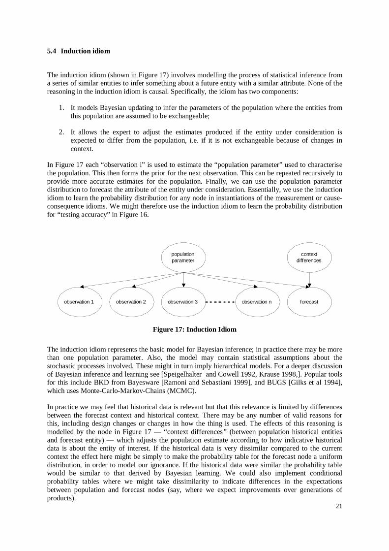
The induction idiom (shown in Figure 17) involves modelling the process of statistical inference from a series of similar entities to infer something about a future entity with a similar attribute. None of the reasoning in the induction idiom is causal. Specifically, the idiom has two components:

1. It models Bayesian updating to infer the parameters of the population where the entities from this population are assumed to be exchangeable;

2. It allows the expert to adjust the estimates produced if the entity under consideration is expected to differ from the population, i.e. if it is not exchangeable because of changes in context.

In Figure 17 each “observation i” is used to estimate the “population parameter” used to characterise the population. This then forms the prior for the next observation. This can be repeated recursively to provide more accurate estimates for the population. Finally, we can use the population parameter distribution to forecast the attribute of the entity under consideration. Essentially, we use the induction idiom to learn the probability distribution for any node in instantiations of the measurement or cause-consequence idioms. We might therefore use the induction idiom to learn the probability distribution for “testing accuracy” in Figure 16.

observation 1

populationparameter

observation 2 observation 3 observation n forecast

contextdifferences

Figure 17: Induction Idiom

The induction idiom represents the basic model for Bayesian inference; in practice there may be more than one population parameter. Also, the model may contain statistical assumptions about the stochastic processes involved. These might in turn imply hierarchical models. For a deeper discussion of Bayesian inference and learning see [Speigelhalter and Cowell 1992, Krause 1998,]. Popular tools for this include BKD from Bayesware [Ramoni and Sebastiani 1999], and BUGS [Gilks et al 1994], which uses Monte-Carlo-Markov-Chains (MCMC).

In practice we may feel that historical data is relevant but that this relevance is limited by differences between the forecast context and historical context. There may be any number of valid reasons for this, including design changes or changes in how the thing is used. The effects of this reasoning is modelled by the node in Figure 17 — “context differences” (between population historical entities and forecast entity) — which adjusts the population estimate according to how indicative historical data is about the entity of interest. If the historical data is very dissimilar compared to the current context the effect here might be simply to make the probability table for the forecast node a uniform distribution, in order to model our ignorance. If the historical data were similar the probability table would be similar to that derived by Bayesian learning. We could also implement conditional probability tables where we might take dissimilarity to indicate differences in the expectations between population and forecast nodes (say, where we expect improvements over generations of products).

22

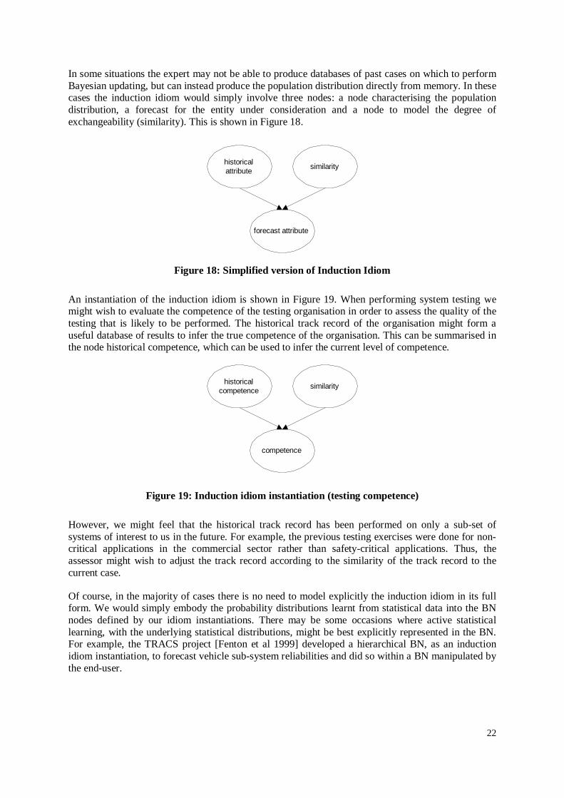
In some situations the expert may not be able to produce databases of past cases on which to perform Bayesian updating, but can instead produce the population distribution directly from memory. In these cases the induction idiom would simply involve three nodes: a node characterising the population distribution, a forecast for the entity under consideration and a node to model the degree of exchangeability (similarity). This is shown in Figure 18.

historicalattribute

forecast attribute

similarity

Figure 18: Simplified version of Induction Idiom

An instantiation of the induction idiom is shown in Figure 19. When performing system testing we might wish to evaluate the competence of the testing organisation in order to assess the quality of the testing that is likely to be performed. The historical track record of the organisation might form a useful database of results to infer the true competence of the organisation. This can be summarised in the node historical competence, which can be used to infer the current level of competence.

historicalcompetence

competence

similarity

Figure 19: Induction idiom instantiation (testing competence)

However, we might feel that the historical track record has been performed on only a sub-set of systems of interest to us in the future. For example, the previous testing exercises were done for non-critical applications in the commercial sector rather than safety-critical applications. Thus, the assessor might wish to adjust the track record according to the similarity of the track record to the current case.

Of course, in the majority of cases there is no need to model explicitly the induction idiom in its full form. We would simply embody the probability distributions learnt from statistical data into the BN nodes defined by our idiom instantiations. There may be some occasions where active statistical learning, with the underlying statistical distributions, might be best explicitly represented in the BN. For example, the TRACS project [Fenton et al 1999] developed a hierarchical BN, as an induction idiom instantiation, to forecast vehicle sub-system reliabilities and did so within a BN manipulated by the end-user.

23

5.5 Reconciliation Idiom

In building BNs we found some difficulty when attempting to model attributes that could be assigned causal probabilities in a BN, but which were also measured by collections of sub-attributes that themselves had uncertain relations with the attribute. For example, we might be interested in the effects of process quality on fault tolerance (a piece of equipment’s ability to tolerate failures in operation) and also the contribution of various fault tolerance strategies that together define fault tolerance, such as error checking and error recovery mechanisms. The challenge here is how to reconcile the equally valid statements p(fault tolerance | process quality) and p(fault tolerance | error recovery, error checking) given that p(fault tolerance | error checking, error recovery, process quality) does not make sense.

The objective of the reconciliation idiom is to reconcile independent sources of evidence about a single attribute of a single entity, where these sources of evidence have been produced by different measurement or prediction methods (i.e. other BNs). The reconciliation idiom is shown in Figure 20.

node X frommodel A

reconciliation

node X frommodel B

Figure 20: Reconciliation idiom

The node of interest, node X, is estimated by two independent procedures, model A and model B. The reconciliation node is a Boolean node. When the reconciliation node is set to ‘true’ the value of X from model A is equal to the value of X from model B. Thus, we allow the flow of evidence from model B to model A. There is, however, one proviso — should both sets of evidence prove contradictory then the inferences cannot obviously be reconciled.

The following example of a reconciliation idiom is typical of many we have come across in safety/reliability assessment. We have two models to estimate the quality of the testing performed on a piece of software:

1. Prediction from known causal factors (represented by a cause-consequence idiom instantiation);

2. Inference from sub-attributes of testing quality which when observed give a partial observation of testing quality (represented by a definitional/synthesis idiom instantiation).

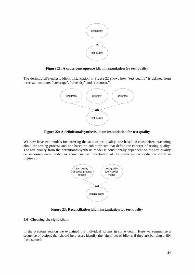
The relevant process product idiom instantiation here is shown in Figure 21 (a complex product will be less easy to test).

24

complexity

test quality

Figure 21: A cause-consequence idiom instantiation for test quality

The definitional/synthesis idiom instantiation in Figure 22 shows how “test quality” is defined from three sub-attributes “coverage”, “diversity” and “resources” .

resources

test quality

diversity coverage

Figure 22: A definitional/synthesis idiom instantiation for test quality

We now have two models for inferring the state of test quality; one based on cause effect reasoning about the testing process and one based on sub-attributes that define the concept of testing quality. The test quality from the definitional/synthesis model is conditionally dependent on the test quality cause-consequence model, as shown in the instantiation of the prediction/reconciliation idiom in Figure 23.

test quality(process-product

model)

reconciliation

test quality(definitional

model)

Figure 23: Reconciliation idiom instantiation for test quality

5.6 Choosing the right idiom

In the previous section we explained the individual idioms in some detail. Here we summarise a sequence of actions that should help users identify the ‘right’ set of idioms if they are building a BN from scratch:

25

1. Make a list of the entities and their attributes, which you believe to be of relevance to your BN.

2. Consider how the entities and attributes relate to one another. This should lead to subsets of entities and attributes grouped together.

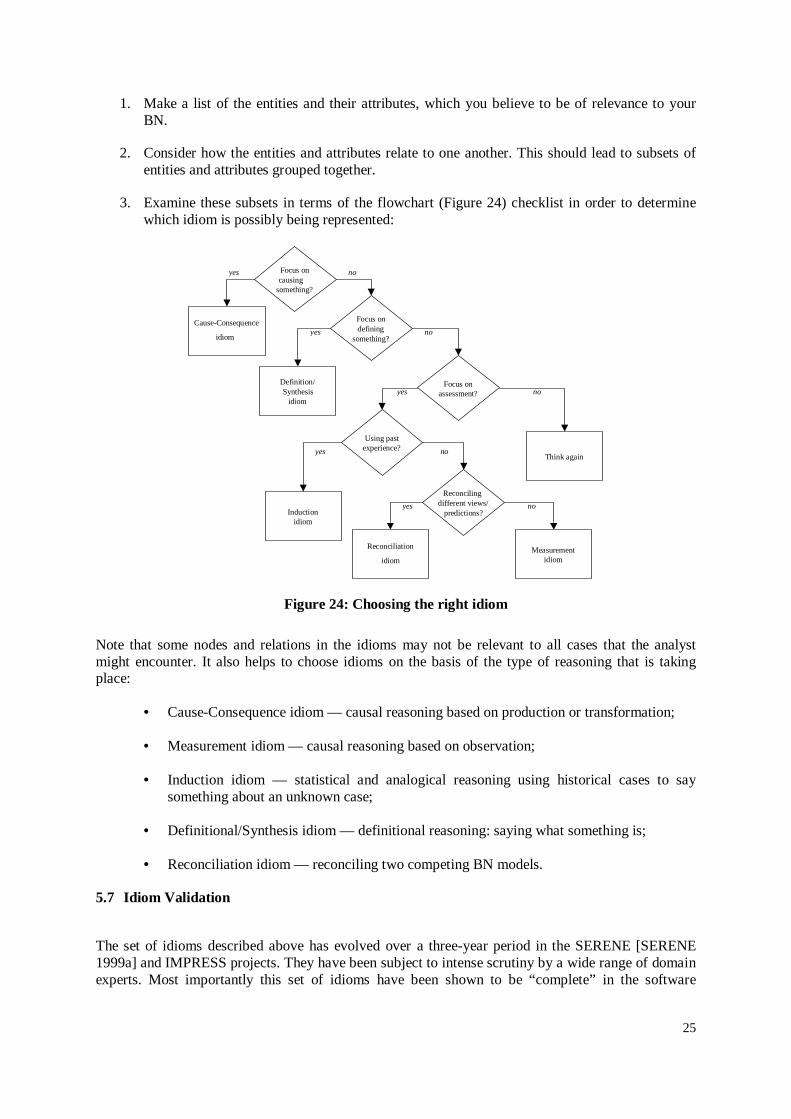
3. Examine these subsets in terms of the flowchart (Figure 24) checklist in order to determine which idiom is possibly being represented:

Focus oncausing

something?

Focus ondefining

something?

Focus onassessment?

Cause-Consequence

idiom

Measurementidiom

Definition/Synthesis

idiom

Inductionidiom

Reconciliation

idiom

Using pastexperience?

Reconcilingdifferent views/

predictions?

Think again

yes no

yes

yes

yes

yes

no

no

no

no

Figure 24: Choosing the right idiom

Note that some nodes and relations in the idioms may not be relevant to all cases that the analyst might encounter. It also helps to choose idioms on the basis of the type of reasoning that is taking place:

• Cause-Consequence idiom — causal reasoning based on production or transformation;

• Measurement idiom — causal reasoning based on observation;

• Induction idiom — statistical and analogical reasoning using historical cases to say something about an unknown case;

• Definitional/Synthesis idiom — definitional reasoning: saying what something is;

• Reconciliation idiom — reconciling two competing BN models.

5.7 Idiom Validation

The set of idioms described above has evolved over a three-year period in the SERENE [SERENE 1999a] and IMPRESS projects. They have been subject to intense scrutiny by a wide range of domain experts. Most importantly this set of idioms have been shown to be “complete” in the software

26

assessment domain in the sense that every BN we have encountered could be constructed in terms of these idioms.

To date these idioms have been applied in:

• safety argumentation for complex software-intensive systems [SERENE 1999c], [Courtois et al 1998], [Neil et al 1996], [Fenton et al 1998];

• software defect density modelling [Fenton and Neil 1999a, Fenton and Neil 1999b, Neil and Fenton 1996];

• software process improvement using statistical process control (SPC) concepts [Lewis 1998];

• vehicle reliability prediction [Fenton et al 1999].

6. Building a BN Using Idioms and Objects

Here we show how to build a fairly large BN using idioms and OOBNs. The example is a cut-down version of a real application developed by Agena Ltd. Some structural and node name changes have been made to protect confidentiality. The application involved predicting the safety risk presented by software based systems. The customer wanted the capability to:

• Predict safety early in the system life-cycle, ideally at the invitation to tender stage;

• Account for information gathered during the development process and from actual test/measurement of the documentation and intermediate products delivered;

• Evaluate the quality of results produced by independent testing organisations that would assess the systems before delivery.

The reader will recognise parts of each of the BNs presented from the idiom instantiations presented in Section 4.

The BN is organised in modules with one core module — the risk BN — and a number of satellite BNs — the severity, supplier, test quality and competence BNs. These modules are then joined together, as objects, to form the safety BN.

The example is sufficiently small to convey the ideas. We have built larger BN models in practice using the same methods but for reasons of limited space we cannot describe them here.

The example uses the SERENE tool to show how the model was constructed.

6.1 The Core Risk BN

The risk BN involves predicting risk from two main sources:

• Test results produced by an independent testing organisation;

• Knowledge of the supplier quality and the difficulty of the problem being solved by the system.

We modelled the process of independent testing using the measurement idiom —

27

p(test results | risk, test quality)

and the cause-consequence idiom —

p(test quality | complexity, competence).

The development process component was modelled using the cause-consequence idiom —

p(failures | problem difficulty, supplier quality) and p(complexity | supplier quality).

Risk is defined as the frequency of failure multiplied by the severity of failure. We modelled this using the definitional/synthesis idiom as

p(safety | severity, failures) = severity×failures.

Figure 25 shows the resulting BN module constructed from these idiom instantiations.

safety

test results

competence

test quality

complexityfailuresseverity

problem difficulty supplier quality

Figure 25: Risk BN

The nodes “severity”, “supplier quality”, “test quality” and “competence” are shared with other modular BNs and hence are shown as input or output nodes.

6.2 Satellite BNs

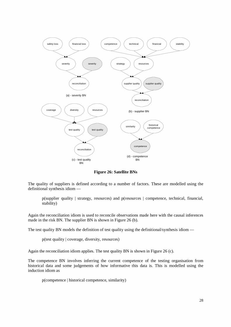
Here we describe the satellite BNs joined to the core BN. Each satellite BN is displayed in Figure 26 (a) to (d).

The first BN is the severity BN and is shown in Figure 26 (a). Here the severity of any failure event was defined from two attributes — financial loss and safety loss (harm to individuals). This was modelled using the definitional/synthesis idiom as

p(severity | safety loss, financial loss)

Also any observations made using this synthesis idiom instantiation must be reconciled with the causal prediction made in the risk BN. Hence we add a reconciliation node with an output node severity. Severity is an output node and is shared with the risk BN.

28

severity

financial losssafety loss

reconciliation

severity

(a) - severity BN

resources

technicalcompetence

reconciliation

supplier quality

financial stability

supplier quality

strategy

(b) - supplier BN

test quality

diversitycoverage

reconciliation

test quality

(c) - test qualityBN

resources

similarity

competence

historicalcompetence

(d) - competenceBN

Figure 26: Satellite BNs

The quality of suppliers is defined according to a number of factors. These are modelled using the definitional synthesis idiom —

p(supplier quality | strategy, resources) and p(resources | competence, technical, financial, stability)

Again the reconciliation idiom is used to reconcile observations made here with the causal inferences made in the risk BN. The supplier BN is shown in Figure 26 (b).

The test quality BN models the definition of test quality using the definitional/synthesis idiom —

p(test quality | coverage, diversity, resources)

Again the reconciliation idiom applies. The test quality BN is shown in Figure 26 (c).

The competence BN involves inferring the current competence of the testing organisation from historical data and some judgements of how informative this data is. This is modelled using the induction idiom as

p(competence | historical competence, similarity)

29

, as shown in Figure 26 (d). Historical competence is used to set a prior distribution on the competence node in the risk BN. It is therefore set as an input node here and as an output node in the risk BN.

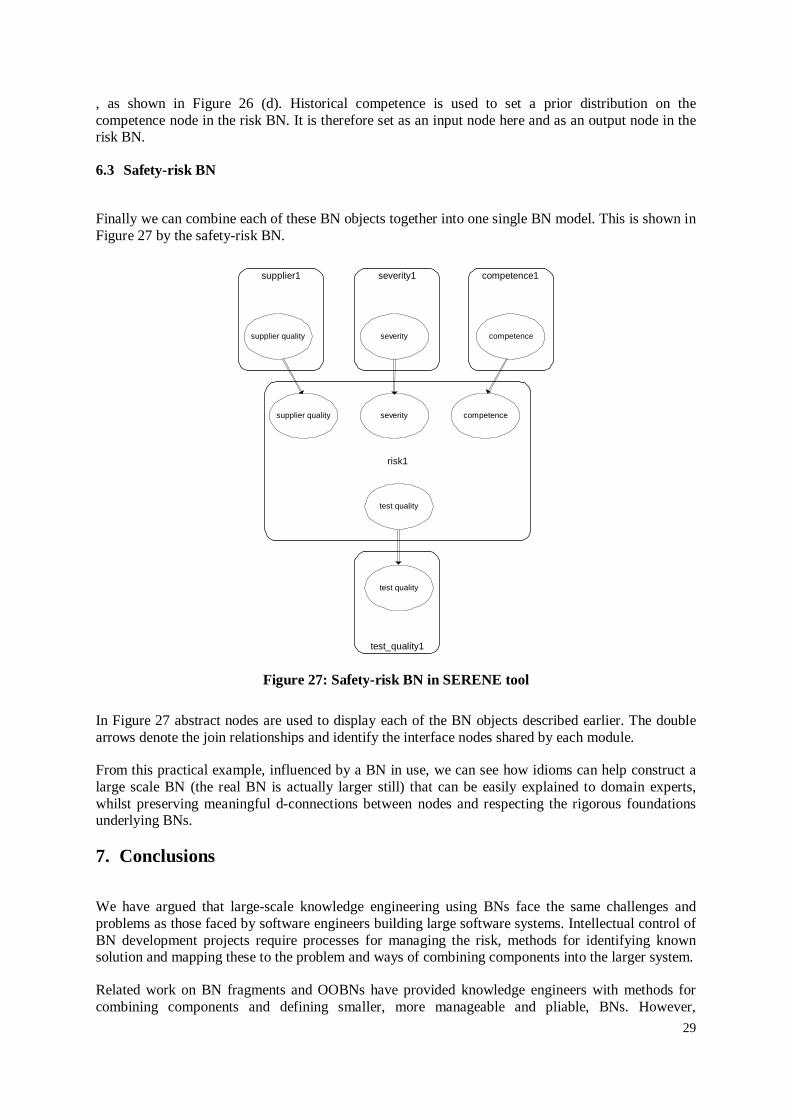
6.3 Safety-risk BN

Finally we can combine each of these BN objects together into one single BN model. This is shown in Figure 27 by the safety-risk BN.

supplier1

risk1

supplier quality severity competence

test quality

supplier quality

severity1

severity

competence1

competence

test_quality1

test quality

Figure 27: Safety-risk BN in SERENE tool

In Figure 27 abstract nodes are used to display each of the BN objects described earlier. The double arrows denote the join relationships and identify the interface nodes shared by each module.

From this practical example, influenced by a BN in use, we can see how idioms can help construct a large scale BN (the real BN is actually larger still) that can be easily explained to domain experts, whilst preserving meaningful d-connections between nodes and respecting the rigorous foundations underlying BNs.

7. Conclusions

We have argued that large-scale knowledge engineering using BNs face the same challenges and problems as those faced by software engineers building large software systems. Intellectual control of BN development projects require processes for managing the risk, methods for identifying known solution and mapping these to the problem and ways of combining components into the larger system.

Related work on BN fragments and OOBNs have provided knowledge engineers with methods for combining components and defining smaller, more manageable and pliable, BNs. However,

30

identification and reuse of patterns of inference have been lacking in past work. We have described a solution to these problems based on the notion of generally applicable “building blocks”, called idioms, which can be combined together into objects. These can then in turn be combined into larger BNs, using simple combination rules and by exploiting recent ideas on OOBNs. This approach, which has been implemented in the SERENE tool can be applied in many problem domains.

The idioms described here have been developed to help practitioners solve one of the major problems encountered when building BNs: that of specifying a sensible graph structure for a BN. Specifically the types of problems encountered in practice involve difficulties in:

• Determining sensible edge directions in the BN given that the direction of inference may run counter to causal direction;

• Applying notions of conditional and unconditional dependence to specify dependencies between nodes;

• Building the BN using a “divide and conquer” approach to manage complexity;

• Reusing experience embodied in previously encountered BN patterns.

In this paper we used an example, drawn from a real BN application, to illustrate how it has been applied to build large-scale BNs for predicting software safety. In addition to this particular application the method has been applied to safety assessment projects, as part of an extensive validation exercise done on the SERENE project, and to other commercial projects in the areas of software quality and vehicle reliability prediction. This experience has demonstrated that relative BN novices can build realistic BN topologies using idioms and OOBNs. Moreover, we are confident that the set of idioms we have defined is sufficient for building BNs in the software safety/reliability domain.

We believe our work forms a major contribution to knowledge engineering practitioners building BN applications. Indeed, we have built working BNs for real applications that we believe are much larger than any previously developed. For example, the TRACS BN [Fenton et al 1999] for a typical vehicle instance contains 350 nodes and over 100 million state combinations.

We expect future advances to come from attempts to overcome the second barrier to the use of BNs: the problem of eliciting probabilities for large conditional probability tables. Our work to date has made some headway in solving this problem through the use of statistical distributions and deterministic functions. By using the equation editor functionality available in the SERENE and Hugin tools we can automatically generate conditional probability tables. We have also been using interpolation methods to generate probability tables using quasi-deterministic rules, coupled with best and worst cases elicited from domain experts. These ideas will be the subject of another paper.

Acknowledgements

This work has been funded by the ESPRIT II project SERENE and the EPSRC project IMPRESS. We would like to thank William Marsh, Frank Jensen, Sven Vestergaard, Asif Makwana, Marc Bouissou, Gunter Gloe and Alain Rouge for their contributions to the SERENE project. We are also very grateful to the referees for their insightful comments and helpful suggestions.

References

[Agena 1999] “Bayesian Belief Nets”, Agena Ltd, Cambridge, UK. Article at http://www.agena.co.uk, 1999.

31

[Boehm 1988] B.W. Boehm. Tutorial on Software Risk Management. IEEE Press, 1988.

[Booch 1993] G. Booch. Object-oriented Analysis and Design with Applications. Benjamin/Cummings, 1993.

[Booch et al 1998] G. Booch, I. Jacobson, J. Rumbaugh. Unified Modeling Language User Guide. Addison Wesley Longman Publishing Co, 1998.

[Cook and Campbell 1979] G.F. Cook and D.T. Campbell. Quasi-Experimentation: Design & analysis for Field Settings. Rand McNally Collge Publishing Co. 1979.

[Courtois et al 1998] P.J. Courtois, N.E. Fenton, B. Littlewood, M. Neil, L. Strigini and D. Wright, “Examination of Bayesian Belief Network for Safety Assessment of Nuclear Computer-based Systems”, DeVa ESPRIT Project 20072, 3rd Year Deliverable, 1998. (Available from the Centre for Software Reliability, City University, Northampton Square, London EC1V 0HB, UK). [Dijkstra 1968] E.W. Dijkstra. “GOTO Considered Harmful”. Comm. ACM, 11, p147-148, 1968. [Dijkstra 1976] E.W Dijkstra. A Discipline of Programming. Englewood Cliffs NJ: Prentice-Hall, 1976.

[Dillan and Goldstein 1984] W. R. Dillan. and M. Goldstein. Multivariate Analysis, Methods and Applications. John E Wiley and Sons, 1984.

[Fenton and Neil 1999a] N. E. Fenton, M. Neil, “Software Metrics: Successes, Failures and New Directions”, Journal of Systems And Software. Vol 47, No.2-3, pp. 149-157, 1999.

[Fenton and Neil 1999b] N.E. Fenton and M. Neil “A Critique of Software Defect Prediction Research”. IEEE Transactions on Software Engineering, Vol. 25, No.3, May/June, 1999.

[Fenton et al 1998] N. Fenton, B. Littlewood, M. Neil, L. Strigini, A. Sutcliffe and D. Wright. “Assessing Dependability of Safety Critical Systems using Diverse Evidence”. IEE Proceedings on Software Engineering, Vol. 145, No.1, February, 1998.

[Fenton et al 1999] N.E. Fenton, M. Neil M and S. Forey. “TRACS (Transport Reliability And Calculation System) User Manual”, CSR/TRACS/D12-v1.0, 30 March 1999. (Available from the Centre for Software Reliability, City University, Northampton Square, London EC1V 0HB, UK).

[Gilks et al 1994] W. R. Gilks, A. Thomas and D. J. Spiegelhalter. “A Language and Program for Complex Bayesian Modelling. The Statistician, 43, 169-78, 1994.

[Hailfinder 1999] Decision systems Laboratory Hailfinder project. http://www.lis.pitt.edu/~dsl/hailfinder/, 1999.

[Heckerman 1990] D. Heckerman. Probabilistic similarity Networks. PhD thesis. Program in Medical Information Sciences, Stanford University, Stanford, CA. Report STAN-CS-90-1316, 1990.

[Heckerman and Horvitz 1998] D. Heckerman and E. Horvitz.. “A Bayesian Approach to Inferring a User's Needs from Free-Text Queries for Assistance”. Gregory F. Cooper and Serafín Moral (editors) Proceedings of the Fourteenth Conference on Uncertainty in Artificial Intelligence, Morgan Kaufmann Publishers, Inc., San Francisco, 1998.

[Hugin 1999] Hugin Expert A/S, Aalborg, Denmark, On-line brochure at http://www.hugin.dk,1999.

[Jackson 1975] M. Jackson. Principles of Program Design. Academia Press, 1975.

[Jackson 1995] M. Jackson. Software Requirements and Specifications: A Lexicon of Practice, Principles and Prejudices. Addison-Wesley/ACM Press, 1995.

[Jensen 1996] F. V. Jensen. An Introduction to Bayesian Networks. UCL Press, London, 1996.

[Koller and Pfeffer 1997] D. Koller and A. Pfeffer. “Object Oriented Bayesian Networks”. Proceedings of the Thirteenth Annual Conference on Uncertainty in Artificial Intelligence. August 1-3, 1997, Brown University, Providence, Rhode Island, USA. Morgan Kaufman Publishers Inc, San Francisco, 1997.

32

[Krause 1998] P. Krause, “Learning Probabilistic Networks”, The Knowledge Engineering Review, Vol. 13 No.4, 1998, pp. 321-351.

[Laskey and Mahoney 1997] K. B. Laskey and S. M. Mahoney “Network Fragments: Representing Knowledge for Constructing Probabilistic Models”. Proceedings of Thirteenth Annual Conference on uncertainty in Artificial Intelligence. Morgan Kaufman Publishers Inc., San Francisco, 1997.

[Lauritzen and Speigelhalter 1988] S.L. Lauritzen and D.J. Spiegelhalter, “Local Computations with Probabilities on Graphical Structures and their Application to Expert Systems (with discussion)”. Journal of the Royal Statistical Society Series B, Vol. 50, No 2, pp.157-224, 1988.

[Lewis 1998] N.D.C. Lewis, ''Continuous Process Improvements using Bayesian Belief Nets; The Lessons to be Learnt'', Proceedings 24th International Conference on Computers and Industrial Engineering, Brunel University, 9-11 September, 1998.

[Mahoney and Laskey 1996] S.M. Mahoney and K.B. Laskey. “Network Engineering for Complex Belief Networks”. Proceedings of Twelfth Annual Conference on Uncertainty in Artificial Intelligence. Morgan Kaufman Publishers Inc., San Francisco, 1996.

[Neil and Fenton 1996] M. Neil and N.E. Fenton, “Predicting Software Quality using Bayesian belief networks”, Proceedings of the 21st Annual Software Engineering Workshop, NASA Goddard Space Flight Centre, pp.217-230, December, 1996.

[Neil et al 1996] M. Neil, B. Littlewood and N. Fenton, “Applying Bayesian Belief Networks to Systems Dependability Assessment”. Proceedings of Safety Critical Systems Club Symposium. Published by Springer-Verlag. Leeds, 6-8 February 1996.

[Parnas 1972] Parnas D.L. ''On the criteria to be used in decomposing systems into modules'', Communications of the ACM, 15(12), 1972, 1052-1058.

[Pearl 1986] Pearl J., “Fusion, propagation, and structuring in belief networks”, Artificial Intelligence, Vol. 29, 1986.

[Pearl 1988] J. Pearl. Probabilistic Reasoning in Intelligent Systems: Networks of Plausible Inference. Morgan Kaufman, 1988.

[Pressman 1992] R.S. Pressman. Software Engineering: A Practitioner’s Approach. McGraw-Hill International, 1992.

[Ramoni and Sebastiani 1999] M. Ramoni and P. Sebastiani. “Learning Conditional Probabilities from Incomplete Data: An Experimental Comparison”, in Proceedings of the Seventh International Workshop on Artificial Intelligence and Statistics, Morgan Kaufman, San Mateo, CA, 1999.

[Rumbaugh et al 1991] J. Rumbaugh, M. Blaha, W. Premerlani, F. Eddy, W. Lorensen. Object-oriented Modeling and Design. Prentice Hall International, 1991

[SERENE 1999a] The SERENE Method Manual Version 1.0 (F), EC Project No. 22187. Project Doc. Number SERENE/5.3/CSR/3053/R/1, 1999. (Available from ERA Technology, Cleeve Road, Leatherhead, Surrey, KT22 7SA, UK).

[SERENE 1999b] The SERENE tool v1.0 available for download from http://www.hugin.dk/serene/

[SERENE 1999c] The SERENE Method Validation Report, EC Project No. 22187, Deliverable Task 5.2 , 1999. (Available from ERA Technology, Cleeve Road, Leatherhead, Surrey, KT22 7SA, UK).

[Shaw and Garland 1996] M. Shaw and D. Garland. Software Architecture,Prentice Hall, 1996

[Sommerville 1992] I. Sommerville. Software Engineering. Addison-Wesley, 1992.

[Speigelhalter and Cowell 1992] D. J. Spegelhalter and R.G. Cowell. “Learning in Probabilistic Expert Systems”, Bayesian Statistics, 4, pp. 447-465. Oxford University Press, 1992.

[Wright and Ayton 1994] G. Wright and P. Ayton (Editors). Subjective Probability. John Wiley and Sons, 1994.