Building counterexamples to generalizations for rational functions of Ritt's decomposition theorem

Journal of Algebra 303 (2006) 655–667

www.elsevier.com/locate/jalgebra

Building counterexamples to generalizations for rationalfunctions of Ritt’s decomposition theorem ✩

Jaime Gutierrez a,∗, David Sevilla b

a Departamento de Matemáticas, Estadística y Computación, Universidad de Cantabria, E-39071 Santander, Spainb Department of Computer Science and Software Engineering, University of Concordia, Montreal, Canada

Received 26 April 2005

Available online 13 July 2006

Communicated by Bruno Salvy

Abstract

The classical Ritt’s theorems state several properties of univariate polynomial decomposition. In thispaper we present new counterexamples to the First Ritt Theorem, which states the equality of length ofdecomposition chains of a polynomial, in the case of rational functions. Namely, we provide an explicitexample of a rational function with coefficients in Q and two decompositions of different length.

Another aspect is the use of some techniques that could allow for other counterexamples, namely, relat-ing groups and decompositions and using the fact that the alternating group A4 has two subgroup chains ofdifferent lengths; and we provide more information about the generalizations of another property of poly-nomial decomposition: the stability of the base field. We also present an algorithm for computing the fixinggroup of a rational function providing the complexity over the rational number field.© 2006 Elsevier Inc. All rights reserved.

Keywords: Ritt’s decomposition theorem; Rational function fields

1. Introduction

The starting point is the decomposition of polynomials and rational functions in one variable.First we will define the basic concepts of this topic.

✩ Partially supported by Spain Ministry of Science grant MTM2004-07086.* Corresponding author.

E-mail address: [email protected] (J. Gutierrez).

0021-8693/$ – see front matter © 2006 Elsevier Inc. All rights reserved.doi:10.1016/j.jalgebra.2006.06.015

656 J. Gutierrez, D. Sevilla / Journal of Algebra 303 (2006) 655–667

Definition 1. If f = g ◦h, f,g,h ∈ K(x), we call this a decomposition of f in K(x) and say thatg is a component on the left of f and h is a component on the right of f . We call a decompositiontrivial if any of the components is a unit with respect to decomposition.

Given two decompositions f = g1 ◦ h1 = g2 ◦ h2 of a rational function, we call them equiva-lent if there exists a unit u such that

h1 = u ◦ h2, g1 = g2 ◦ u−1,

where the inverse is taken with respect to composition.Given a non-constant f , we say that it is indecomposable if it is not a unit and all its decom-

positions are trivial.We define a complete decomposition of f to be f = g1 ◦ · · · ◦gr where gi is indecomposable.

The notion of equivalent complete decompositions is straightforward from the previous concepts.Given a non-constant rational function f (x) ∈ K(x) where f (x) = fN(x)/fD(x) with

fN,fD ∈ K[x] and (fN ,fD) = 1, we define the degree of f as

degf = max{degfN, degfD}.

We also define dega = 0 for each a ∈ K.

Remark 2. From now on, we will use the previous notation when we refer to the numerator anddenominator of a rational function. Unless explicitly stated, we will take the numerator to bemonic, even though multiplication by constants will not be relevant.

The first of Ritt’s theorems states that all the decomposition chains of a polynomial that sat-isfies a certain condition have the same length. Here we explore new techniques related to this,and include a counterexample in Q(x).

Another result in this fashion states that if a polynomial is indecomposable in a certain coef-ficient field, then it is also indecomposable in any extension of that field. This is also false forrational functions, see [4] and [1]. We look for bounds for the degree of the extension in whichwe need to take the coefficients if a rational function with coefficients in Q has a decomposi-tion in a larger field. In this paper we present a computational approach to this question and ourconclusions.

In Section 2 we study how to compute bounds for the minimal field that contains all thedecompositions of a given rational function. In Section 3 we introduce several definitions andproperties of groups related to rational functions, which we use in Section 4 to discuss the numberof components in the rational case. In particular, we present an algorithm for computing fixinggroup of a rational function and we provide the complexity over the rational number field. Finally,in Section 4 we present an example of a degree 12 rational function with coefficients in Q andtwo decompositions of different length; as far as we know this is the first example in Q of thiskind.

2. Extension of the coefficient field

Several algorithms for decomposing univariate rational functions are known, see, for instance,[18] and [1]. In all cases, the complexity of the algorithm grows enormously when the coefficientfield is extended. A natural question about decomposition is whether it depends on the coefficient

J. Gutierrez, D. Sevilla / Journal of Algebra 303 (2006) 655–667 657

field, that is, the existence of polynomials or rational functions that are indecomposable in K(x)

but have a decomposition in F(x) for some extension F of K. Polynomials behave well undercertain conditions, however in the rational case this is not true. We will try to shed some light onthe rational case.

Definition 3. f ∈ K[x] is tame when char K does not divide degf .

The next theorem shows that tame polynomials behave well under extension of the coefficientfield, see [8]. It is based on the concept of approximate root of a polynomial, which always existsfor tame polynomials, and is also the key to some other structural results in the tame polynomialcase.

Theorem 4. Let f ∈ K[x] be tame and F ⊇ K. Then f is indecomposable in K[x] if and only ifit is indecomposable in F[x].

The next example, presented in [1], shows that the previous result is false for rational func-tions.

Example 5. Let

f = ω3x4 − ω3x3 − 8x − 1

2ω3x4 + ω3x3 − 16x + 1,

where ω /∈ Q but ω3 ∈ Q \ {1}. It is easy to check that f is indecomposable in Q(x). However,f = f1 ◦ f2 where

f1 = x2 + (4 − ω)x − ω

2x2 + (8 + ω)x + ω, f2 = xω(xω − 2)

xω + 1.

We can pose the following general problem:

Problem 6. Given a function f ∈ K(x), compute a minimal field F such that every decompositionof f over an extension of K is equivalent to a decomposition over F.

It is clear that, by composing with units in F(x) ⊇ K(x), we can always turn a given de-composition in K(x) into one in F(x). Our goal is to minimize this, that is, to determine fieldsthat contain the smallest equivalent decompositions in the sense of having the smallest possibleextension over K.

Given a decomposition f = g(h) of a rational function in K(x), we can write a polyno-mial system of equations in the coefficients of f , g and h by equating to zero the numerator off − g(h). The system is linear in the coefficients of g. Therefore, all the coefficients of g and h

lie in some algebraic extension of K. Our goal is to find bounds for the degree of the extension[F : K] where F contains, in the sense explained above, all the decompositions of f .

One way to find a bound is by means of a result that relates decomposition and factorization.We state the main definition and theorems here, see [9] for proofs and other details.

Definition 7. A rational function f ∈ K(x) is in normal form if degfN > degfD and fN(0) = 0(thus fD(0) �= 0).


Theorem 8.

(i) Given f ∈ K(x), if degf < |K| then there exist units u, v such that u ◦ f ◦ v is in normalform.

(ii) If f ∈ K(x) is in normal form, every decomposition of f is equivalent to one where bothcomponents are in normal form.

We will analyze the complexity of finding the units u and v later.

Theorem 9. Let f = g(h) with f , g, h in normal form. Then hN divides fN and hD divides fD .

This result provides the following bound.

Theorem 10. Let f ∈ K(x) and u1, u2 be two units in K(x) such that g = u1 ◦ f ◦ u2 is innormal form. Let F be the splitting field of {gN,gD}. Then any decomposition of f in K′(x), forany K′ ⊃ K is equivalent to a decomposition in F(x).

Proof. By Theorems 8 and 9, every decomposition of g is equivalent to another one, g = h1 ◦h2,where the numerator and denominator of h2 divide those of g, thus the coefficients of that com-ponent are in F. As the coefficients of h1 are the solution of a linear system of equations whosecoefficients are polynomials in the coefficients of g and h2, they are also in F. We also haveu1, u2 ∈ K(x), therefore the corresponding decomposition of f lies in the same field. �

This bound, despite being of some interest because its generality and simplicity, is far fromoptimal. For example, for degree 4 we obtain [F : K] � 3! · 3! = 36. The following theoremcompletes Example 5.

Theorem 11. Let f ∈ Q(x) of degree 4. If f = g(h) with g,h ∈ Q(x), there exists a field K withQ ⊂ K ⊂ Q and a unit u ∈ K(x) such that g(u−1), u(h) ∈ K(x) and [K : Q] � 3.

The proof is a straightforward application of Gröbner bases and the well-known ExtensionTheorem, see, for instance, [3].

3. Fixing group and fixed field

In this section we introduce several simple notions from classical Galois theory. Let Γ (K) =AutKK(x) (we will write simply Γ if there can be no confusion about the field). The elementsof Γ (K) can be identified with the images of x under the automorphisms, that is, with Möbiustransformations (non-constant rational functions of the form (ax + b)/(cx + d)), which are alsothe units of K(x) under composition.

Definition 12.

(i) Let f ∈ K(x). We define G(f ) = {u ∈ Γ (K): f ◦ u = f }.(ii) Let H < Γ (K). We define Fix(H) = {f ∈ K(x): f ◦ u = f ∀u ∈ H }.Example 13.

(i) Let f = x2 + 1/x2 ∈ K(x). Then G(f ) = {x,−x,1/x,−1/x}.(ii) Let H = {x, ix,−x,−ix} ⊂ Γ (C). Then Fix(H) = C(x4).


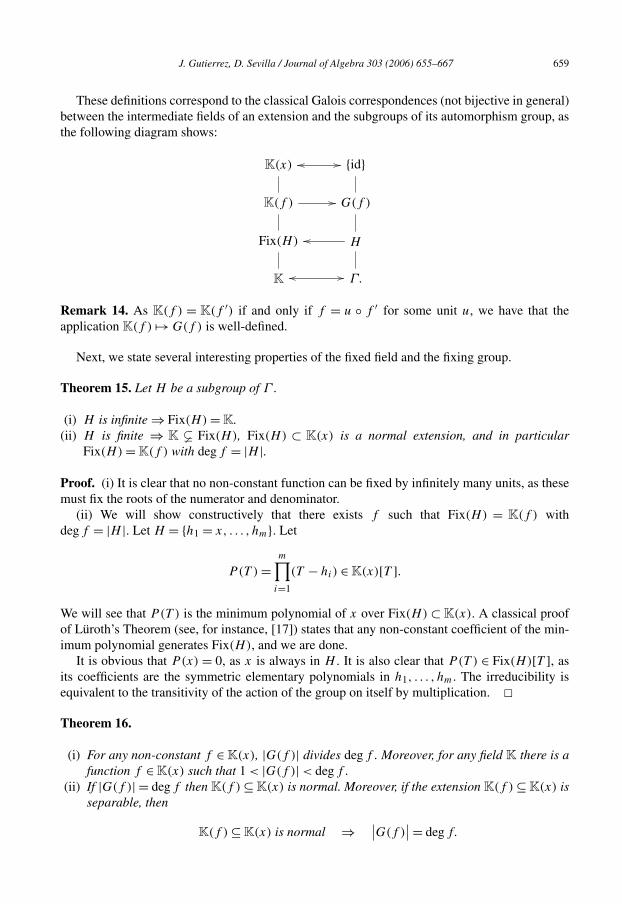
These definitions correspond to the classical Galois correspondences (not bijective in general)between the intermediate fields of an extension and the subgroups of its automorphism group, asthe following diagram shows:

K(x) {id}

K(f ) G(f )

Fix(H) H

K Γ.

Remark 14. As K(f ) = K(f ′) if and only if f = u ◦ f ′ for some unit u, we have that theapplication K(f ) �→ G(f ) is well-defined.

Next, we state several interesting properties of the fixed field and the fixing group.

Theorem 15. Let H be a subgroup of Γ .

(i) H is infinite ⇒ Fix(H) = K.(ii) H is finite ⇒ K � Fix(H), Fix(H) ⊂ K(x) is a normal extension, and in particular

Fix(H) = K(f ) with degf = |H |.

Proof. (i) It is clear that no non-constant function can be fixed by infinitely many units, as thesemust fix the roots of the numerator and denominator.

(ii) We will show constructively that there exists f such that Fix(H) = K(f ) withdegf = |H |. Let H = {h1 = x, . . . , hm}. Let

P(T ) =m∏

i=1

(T − hi) ∈ K(x)[T ].

We will see that P(T ) is the minimum polynomial of x over Fix(H) ⊂ K(x). A classical proofof Lüroth’s Theorem (see, for instance, [17]) states that any non-constant coefficient of the min-imum polynomial generates Fix(H), and we are done.

It is obvious that P(x) = 0, as x is always in H . It is also clear that P(T ) ∈ Fix(H)[T ], asits coefficients are the symmetric elementary polynomials in h1, . . . , hm. The irreducibility isequivalent to the transitivity of the action of the group on itself by multiplication. �Theorem 16.

(i) For any non-constant f ∈ K(x), |G(f )| divides degf . Moreover, for any field K there is afunction f ∈ K(x) such that 1 < |G(f )| < degf .

(ii) If |G(f )| = degf then K(f ) ⊆ K(x) is normal. Moreover, if the extension K(f ) ⊆ K(x) isseparable, then

K(f ) ⊆ K(x) is normal ⇒ ∣∣G(f )∣∣ = degf.


(iii) Given a finite subgroup H of Γ , there is a bijection between the subgroups of H and thefields between Fix(H) and K(x). Also, if Fix(H) = K(f ), there is a bijection between theright components of f (up to equivalence by units) and the subgroups of H .

Proof. (i) The field Fix(G(f )) is between K(f ) and K(x), therefore the degree of any generator,which is the same as |G(f )|, divides degf . For the second part, take for example f = x2(x−1)2,which gives G(f ) = {x,1 − x} in any coefficient field.

(ii) The elements of G(f ) are the roots of the minimum polynomial of x over K(f ) that arein K(x). If there are degf different roots, as this number equals the degree of the extension weconclude that it is normal.

If K(f ) ⊂ K(x) is separable, all the roots of the minimum polynomial of x over K(f ) aredifferent, thus if the extension is normal there are as many roots as the degree of the extension.

(iii) Due to Theorem 15, the extension Fix(H) ⊂ K(x) is normal, and the result is a conse-quence of the Fundamental Theorem of Galois. �Remark 17. K(x) is Galois over K (that is, the only rational functions fixed by Γ (K) are theconstant ones) if and only if K is infinite. Indeed, if K is infinite, for each non-constant functionf there exists a unit x + b with b ∈ K which does not leave it fixed. On the other hand, if K

is finite then Γ (K) is finite too, and the proof of Theorem 15 provides a non-constant rationalfunction that generates Fix(Γ (K)).

Algorithms for computing several aspects of Galois theory can be found in [16]. Unfor-tunately, it is not true in general that [K(x) : K(f )] = |G(f )|; there is no bijection betweenintermediate fields and subgroups of the fixing group of a given function. Anyway, we can obtainpartial results on decomposability.

Theorem 18. Let f be indecomposable.

(i) If degf is prime, then either G(f ) is cyclic of order degf , or it is trivial.(ii) If degf is composite, then G(f ) is trivial.

Proof. (i) If 1 < |G(f )| < degf , we have K(f ) � K(Fix(G(f ))) � K(x) and any generator ofK(Fix(G(f ))) is a proper component of f on the right. Therefore, G(f ) has order either 1 ordegf , and in the latter case, being prime, the group is cyclic.

(ii) Assume G(f ) is not trivial. If |G(f )| < degf , we have a contradiction as in (i). If|G(f )| = degf , as it is a composite number, there exists H � G(f ) not trivial, and again anygenerator of Fix(H) is a proper component of f on the right. �Corollary 19. If f has composite degree and G(f ) is not trivial, f is decomposable.

Now we present algorithms to efficiently compute fixed fields and fixing groups.The proof of Theorem 15 provides an algorithm to compute a generator of Fix(H) from its

elements.

Algorithm 1.

INPUT: H = {h1, . . . , hm} < Γ (K).OUTPUT: f ∈ K(x) such that Fix(H) = K(f ).


A. Let i = 1.B. Compute the ith symmetric elementary function σi(h1, . . . , hm).C. If σi(h1, . . . , hm) /∈ K, return σi(h1, . . . , hm). If it is constant, increase i and return to B.

We illustrate this algorithm with the following example.

Example 20. Let

H ={±x ,± 1

x,± i(x + 1)

x − 1,± i(x − 1)

x + 1,±x + i

x − i,±x − i

x + i

}< Γ (C).

Then

P(T ) = T 12 − x12 − 33x8 − 33x4 + 1

x2(x − 1)2(x + 1)2(x4 + 2x2 + 1)T 10 − 33T 8

+ 2x12 − 33x8 − 33x4 + 1

x2(x − 1)2(x + 1)2(x4 + 2x2 + 1)T 6 − 33T 4

− x12 − 33x8 − 33x4 + 1

x2(x − 1)2(x + 1)2(x4 + 2x2 + 1)T 2 + 1.

Thus,

Fix(H) = C

(x12 − 33x8 − 33x4 + 1

x2(x − 1)2(x + 1)2(x4 + 2x2 + 1)

).

H is isomorphic to A4. It is known that A4 has two complete subgroup chains of different lengths:

{id} ⊂ C2 ⊂ V ⊂ A4, {id} ⊂ C3 ⊂ A4.

In our case,

{x} ⊂ {±x} ⊂{±x,± 1

x

}⊂ H, {x} ⊂

{x,

x + i

x − i,i(x + 1)

x − 1

}⊂ H.

Applying our algorithm again we obtain the following field chains:

C(f ) ⊂ C

(x2 + 1

x2

)⊂ C

(x2) ⊂ C(x),

C(f ) ⊂ C

(−i(t + i)(1 + t)t

(−t + i)(−1 + t)

)⊂ C(x).

As there is a bijection in this case, the corresponding two decompositions are complete.

In order to compute the fixing group of a function f we can solve the system of polynomialequations obtained from

f

(ax + b

)= f (x).

cx + d


This can be reduced to solving two simpler systems, those given by

f (ax + b) = f (x) and f

(ax + b

x + d

)= f (x).

This method is simple but inefficient; we will describe another method that is faster in practice.We need to assume that K has sufficiently many elements. If not, we take an extension of K

and later we check which of the computed elements are in Γ (K) by solving simple systems oflinear equations.

Theorem 21. Let f ∈ K(x) of degree m in normal form and u = ax+bcx+d

such that f ◦ u = f .

(i) a �= 0 and d �= 0.(ii) fN(b/d) = 0.

(iii) If c = 0 (that is, we take u = ax + b), then fN(b) = 0 and am = 1.(iv) If c �= 0 then fD(a/c) = 0.

Proof. (i) Suppose a = 0. We can assume u = 1/(cx + d) = (1/x) ◦ (cx + d) But if we considerf (1/x), its numerator has smaller degree than its denominator. As composing on the right withcx + d does not change those degrees, it is impossible that f ◦ u = f . Also, as the inverse of u

is dx−b−cx+a

, we have d �= 0.

(ii) Let

f = amxm + · · · + a1x

bm−1xm−1 + · · · + b0.

The constant term of the numerator of f ◦ u is

ambm + am−1bm−1d + · · · + a1bdm−1 = dmfN(b/d).

As d �= 0 by (i), we have that fN(b/d) = 0. Alternatively, 0 = f (0) = (f ◦ u)(0) = f (u(0)) =f (b/d).

(iii), (iv) They are similar to the previous item. �We can use this theorem to compute the polynomial and rational elements of G(f ) separately.

Algorithm 2.

INPUT: f ∈ K(x).OUTPUT: G(f ) = {w ∈ K(x) : f ◦ w = f }.

A. Compute units u,v such that f̄ = u ◦ f ◦ v is in normal form. Let m = degf . Let L be anempty list.

B. Compute A = {α ∈ K: αm = 1}, B = {β ∈ K: f̄N (β) = 0} and C = {γ ∈ K: f̄D(γ ) = 0}.C. For each (α,β) ∈ A × B , check if f̄ (αx + β) = f̄ (x). In that case add ax + b to L.D. For each (β, γ ) ∈ B × C, let w = cγ x+β

c x+1 . Compute all values of c for which f̄ ◦ w = f̄ . Foreach solution, add the corresponding unit to L.

E. Let L = {w1, . . . ,wk}. Return {v ◦ wi ◦ v−1: i = 1, . . . , k}.


Analysis. It is clear that the cost of the algorithm heavily depends on the complexity of the bestalgorithm to compute the roots of a univariate polynomial in the given field. We analyze thebit complexity when the ground field is the rational number Q. We will use several well-knownresults about complexity, those can be consulted in the book [7].

In the following, M denotes a multiplication time, so that the product of two polynomialsin K[x] with degree at most m can be computed with at most M(m) arithmetic operations. IfK supports the Fast Fourier Transform, several known algorithms require O(n logn log logn)

arithmetic operations. We denote by l(f ) the maximum norm of f , that is, l(f ) = ‖f ‖∞ =max |ai | of a polynomial f = ∑

i aixi ∈ Z[x].

Polynomials in f,g ∈ Z[x] of degree less than m can be multiplied using O(M(m(l+ logm)))

bit operations, where l = log max(l(f ), l(g)).Now, suppose that the given polynomial f is squarefree primitive, then we can compute all

its rational roots with an expected number of T (m, log l(f )) bit operations, where

T(m, log l(f )

) = O(m log

(ml(f )

))(log2 log logm + (

log log l(f ))2 log log log l(f )

)+ m2M

(log

(ml(f )

)).

We discuss separately the algorithm steps. Let f = fN/fD , where fN,fD ∈ Z[x] and let l =log max(l(fN), l(gD)) and m = degf .

Step A. Let u ∈ Q(x) be a unit such that gN/gD = u(f ) with deggN > deggD . Such a unitalways exists:

– If degfN = degfD . Let u = 1/(x − a), where a ∈ Q verifies degfN − a degfD < degfN .– If degfN < degfD , let u = 1/x.

Now, let b ∈ Z such that gD(b) �= 0. Then hN/hD = gN(x + b)/gD(x + b) verifies hD(0) �= 0and the rational function (x −h(0))◦hN/hD is in normal form. Obviously, the complexity in thisstep is dominated on choosing b. In the worst case, we have to evaluate the integers 0,1, . . . ,m

in gD . Clearly, a complexity bound is O(M(m3l)).

Step B. Compute the set A can be done on constant time. Now, in order to compute the com-plexity, we can suppose, without loss of generality, that fN and fD are squarefree and primitive.Then the bit complexity to compute both set B and set C is T (m,ml).

Step C. A bound for the cardinal of A is 4 and m for the cardinal of B . Then, we need tocheck 4m times if f̄ (αx + β) = f̄ (x) for each (α,β) ∈ A × B . So, the complexity of this step isbounded by O(M(m4l)).

Step D. In the worst case the cardinal of B × C is m2. This step requires to compute all rationalroots of m2 polynomials h(x) given by the equation:

f̄ ◦ w = f̄ ,

for each (β, γ ) ∈ B × C, where w = cγ x+βcx+1 . A bound for the degree of h(x) is m2. The size of

the coefficients is bounded by ml, so a bound for total complexity of this step is m4T (m2, lm2).


Step E. Finally, this step requires substituting at most 2m rational functions of degree m and thecoefficients size is bounded by lm3. So, abound for the complexity is O(M(m4l)).

We can conclude that the complexity of this algorithm is dominated by that of Step D, that is,m4T (m2, lm2). Of course, a worst bound for this is O(m8l2).

The following example illustrates the above algorithm.

Example 22. Let

f = (−3x + 1 + x3)2

x(−2x − x2 + 1 + x3)(−1 + x)∈ Q(x).

We normalize f : let u = 1x−9/2 and v = 1

x− 1, then

f̄ = u ◦ f ◦ v = −4x6 − 6x5 + 32x4 − 34x3 + 14x2 − 2x

27x5 − 108x4 + 141x3 − 81x2 + 21x − 2

is in normal form.The roots of the numerator and denominator of f̄ in Q are {0,1,1/2} and {1/3,2/3}, respec-

tively. The only sixth roots of unity in Q are 1 and −1; as charQ = 0 there cannot be elementsof the form x + b in G(f̄ ). Thus, there are two polynomial candidates: −x + 1/3, −x + 2/3.A quick computation reveals that none of them fixes f̄ .

Let w = cβx+αcx+1 . As α ∈ {0,1,1/2} and β ∈ {1/3,2/3}, another quick computation shows that

G(f̄ ) ={x,

−x + 1

−3x + 2,−2x + 1

−3x + 1

}

and

G(f ) = v · G(f̄ ) · v−1 ={x,

1

1 − x,x − 1

x

}.

From this group we can compute a proper component of f as in the proof of Theorem 18,obtaining f = g(h) with

h = −3x + 1 + x3

(−1 + x)x, g = x2

x − 1.

In the next section we will use these tools to investigate the number of components of arational function.

4. Ritt’s Theorem and number of components

One of the classical Ritt’s theorems (see [13]) describes the relation among the different de-composition chains of a tame polynomial. Essentially, all the decompositions have the samelength and are related in a rather simple way.


Definition 23. A bidecomposition is a 4-tuple of polynomials f1, g1, f2, g2 such that f1 ◦ g1 =f2 ◦ g2, degf1 = degg2 and (degf1,degg1) = 1.

Theorem 24 (Ritt’s First Theorem). Let f ∈ K[x] be tame and

f = g1 ◦ · · · ◦ gr = h1 ◦ · · · ◦ hs

be two complete decomposition chains of f . Then r = s, and the sequences (degg1, . . . ,deggr),(degh1, . . . ,deghs) are permutations of each other. Moreover, there exists a finite chain of com-plete decompositions

f = f(j)

1 ◦ · · · ◦ f(j)r , j ∈ {1, . . . , k},

such that

f(1)i = gi, f

(k)i = hi, i = 1, . . . , r,

and for each j < k, there exists ij such that the j th and (j + 1)th decomposition differ only inone of these aspects:

(i) f(j)ij

◦ f(j)

ij +1 and f(j+1)ij

◦ f(j+1)

ij +1 are equivalent.

(ii) f(j)ij

◦ f(j)

ij +1 = f(j+1)ij

◦ f(j+1)

ij +1 is a bidecomposition.

Proof. See [13] for K = C, [5] for characteristic zero fields and [6,15] for the general case. �Unlike for polynomials, it is not true that all complete decompositions of a rational function

have the same length, as shown in Example 20. The paper [10] presents a detailed study of thisproblem for non-tame polynomial with coefficients over a finite field. The problem for rationalfunctions is strongly related to the open problem of the classes of rational functions which com-mute with respect to composition, see [14]. In this section we will give some ideas about therelation between complete decompositions and subgroup chains that appear by means of Galoistheory.

Now we present another degree 12 function, this time with coefficients in Q, that has twocomplete decomposition chains of different length. This function arises in the context of Mon-strous Moonshine as a rational relationship between two modular functions (see, for example, theclassical [2] for an overview of this broad topic, or Ref. [12], in Spanish, for the computations inwhich this function appears).

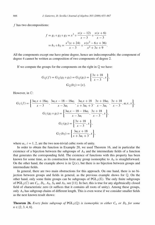
Example 25. Let f ∈ Q(x) be the following degree 12 function:

f = x3(x + 6)3(x2 − 6x + 36)3

(x − 3)3(x2 + 3x + 9)3.


f has two decompositions:

f = g1 ◦ g2 ◦ g3 = x3 ◦ x(x − 12)

x − 3◦ x(x + 6)

x − 3

= h1 ◦ h2 = x3(x + 24)

x − 3◦ x(x2 − 6x + 36)

x2 + 3x + 9.

All the components except one have prime degree, hence are indecomposable; the component ofdegree 4 cannot be written as composition of two components of degree 2.

If we compute the groups for the components on the right in Q we have:

GQ(f ) = GQ(g2 ◦ g3) = GQ(g3) ={

3x + 18

x − 3, x

},

GQ(h2) = {x}.

However, in C:

GC(f ) ={

3αix + 18αi

x − 3,

3αix − 18 − 18αi

x − 3αi

,3αix + 18

x + 3αi + 3,

3x + 18αi

x − 3αi

,3x + 18

x − 3, αix, x

},

GC(g2 ◦ g3) ={

3αix − 18 − 18αi

x − 3αi

,3x + 18

x − 3, x

},

GC(g3) ={

3x + 18

x − 3, x

},

GC(h2) ={

3αix + 18

x + 3αi + 3, x

},

where αi , i = 1,2, are the two non-trivial cubic roots of unity.In order to obtain the function in Example 20, we used Theorem 16, and in particular the

existence of a bijection between the subgroups of A4 and the intermediate fields of a functionthat generates the corresponding field. The existence of functions with this property has beenknown for some time, as its construction from any group isomorphic to A4 is straightforward.On the other hand, the example above is in Q(x), but there is no bijection between groups andintermediate fields.

In general, there are two main obstructions for this approach. On one hand, there is no bi-jection between groups and fields in general, as the previous example shows for Q. On theother hand, only some finite groups can be subgroups of PGL2(K). The only finite subgroupsof PGL2(C) are Cn, Dn, A4, S4 and A5, see [11]. In fact, this is true for any algebraically closedfield of characteristic zero (it suffices that it contains all roots of unity). Among these groups,only A4 has subgroup chains of different length. This is even worse if we consider smaller fieldsas the next known result shows:

Theorem 26. Every finite subgroup of PGL2(Q) is isomorphic to either Cn or Dn for somen ∈ {2,3,4,6}.


Indeed these all occur, unfortunately none of them has two subgroup chains of differentlengths, so no new functions can be found in this way.

5. Conclusions

In this paper we have presented several counterexamples to the generalization of the FirstRitt Theorem to rational functions. We also introduced and analyzed several concepts of Galoistheory that we expect to be interesting in providing more structural information in this topic.Also, we show a use of techniques from computational algebra results to find bounds for the sizeof a field that contains all decompositions of a given function; we expect that general propertiesof Gröbner bases can be applied to this end in order to obtain general bounds.

References

[1] C. Alonso, J. Gutierrez, T. Recio, A rational function decomposition algorithm by near-separated polynomials,J. Symbolic Comput. 19 (6) (1995) 527–544.

[2] J.H. Conway, S.P. Norton, Monstrous moonshine, Bull. London Math. Soc. 11 (1979) 308–339.[3] D. Cox, J. Little, D. O’Shea, Ideals, Varieties and Algorithms: An Introduction to Computational Algebraic Geom-

etry and Commutative Algebra, Springer-Verlag, New York, 1997.[4] F. Dorey, G. Whaples, Prime and composite polynomials, J. Algebra 28 (1974) 88–101.[5] H.T. Engström, Polynomial substitutions, Amer. J. Math. 63 (1941) 249–255.[6] M. Fried, R. MacRae, On the invariance of chains of fields, Illinois J. Math. 13 (1969) 165–171.[7] J. von zur Gathen, J. Gerhard, Modern Computer Algebra, Cambridge Univ. Press, New York, 1999.[8] J. Gutierrez, A polynomial decomposition algorithm over factorial domains, C. R. Math. Rep. Acad. Sci.

Canada 13 (2–3) (1991) 81–86.[9] J. Gutierrez, R. Rubio, D. Sevilla, Unirational fields of transcendence degree one and functional decomposition, in:

Proceedings of ISSAC 2001, London, Canada, pp. 167–174.[10] J. Gutierrez, D. Sevilla, On Ritt’s decomposition theorem in the case of finite fields, Finite Fields Appl. 12 (2006)

403–412.[11] F. Klein, The Icosahedron: And the Solution of Equations of the Fifth Degree, Dover, New York, 1956.[12] J. McKay, D. Sevilla, Application of univariate rational decomposition to Monstrous Moonshine, in: Proceedings

of EACA, 2004, pp. 289–294 (in Spanish).[13] J.F. Ritt, Prime and composite polynomials, Trans. Amer. Math. Soc. 23 (1) (1922) 51–66.[14] J.F. Ritt, Permutable rational functions, Trans. Amer. Math. Soc. 25 (3) (1923) 399–448.[15] A. Schinzel, Polynomials with Special Regard to Reducibility, Cambridge Univ. Press, New York, 2000.[16] A. Valibouze, Computation of the Galois groups of the resolvent factors for the direct and inverse Galois problems,

in: Proc. Applied Algebra, Algebraic Algorithms and Error-Correcting Codes, Paris, 1995, in: Lecture Notes inComput. Sci., vol. 948, 1995, pp. 456–468.

[17] B.L. van der Waerden, Modern Algebra, Frederick Ungar Publishing Co., New York, 1964.[18] R. Zippel, Rational function decomposition, in: Proc. ISSAC ’91, ACM Press, 1991, pp. 1–6.

Building counterexamples to generalizations for rational functions of Ritt's decomposition theorem

Documents

Transcript of Building counterexamples to generalizations for rational functions of Ritt's decomposition theorem