Building Blocks for Variational Bayesian Learning of ...
47
Journal of Machine Learning Research 8 (2007) 155-201 Submitted 11/04; Revised 12/05; Published 1/07 Building Blocks for Variational Bayesian Learning of Latent Variable Models Tapani Raiko TAPANI .RAIKO@HUT. FI Harri Valpola HARRI .VALPOLA@HUT. FI Markus Harva MARKUS.HARVA@HUT. FI Juha Karhunen J UHA.KARHUNEN@HUT. FI Adaptive Informatics Research Centre Helsinki University of Technology P.O.Box 5400, FI-02015 HUT, Espoo, Finland Editor: Michael I. Jordan Abstract We introduce standardised building blocks designed to be used with variational Bayesian learning. The blocks include Gaussian variables, summation, multiplication, nonlinearity, and delay. A large variety of latent variable models can be constructed from these blocks, including nonlinear and variance models, which are lacking from most existing variational systems. The introduced blocks are designed to fit together and to yield efficient update rules. Practical implementation of various models is easy thanks to an associated software package which derives the learning formulas au- tomatically once a specific model structure has been fixed. Variational Bayesian learning provides a cost function which is used both for updating the variables of the model and for optimising the model structure. All the computations can be carried out locally, resulting in linear computational complexity. We present experimental results on several structures, including a new hierarchical nonlinear model for variances and means. The test results demonstrate the good performance and usefulness of the introduced method. Keywords: latent variable models, variational Bayesian learning, graphical models, building blocks, Bayesian modelling, local computation 1. Introduction Various generative modelling approaches have provided powerful statistical learning methods for neural networks and graphical models during the last years. Such methods aim at finding an ap- propriate model which explains the internal structure or regularities found in the observations. It is assumed that these regularities are caused by certain latent variables (also called factors, sources, hidden variables, or hidden causes) which have generated the observed data through an unknown mapping (Bishop, 1999). In unsupervised learning, the goal is to identify both the unknown latent variables and generative mapping. The expectation-maximisation (EM) algorithm (Dempster et al., 1977) has often been used for learning latent variable models. The distribution for the latent variables is modelled, but the model parameters are found using maximum likelihood or maximum a posteriori estimators. However, with such point estimates, determination of the correct model order and overfitting are ubiquitous and often difficult problems. Therefore, full Bayesian approaches making use of the complete poste- rior distribution have recently gained a lot of attention. Exact treatment of the posterior distribution c 2007 Tapani Raiko, Harri Valpola, Markus Harva and Juha Karhunen.
Transcript of Building Blocks for Variational Bayesian Learning of ...

Journal of Machine Learning Research 8 (2007) 155-201 Submitted 11/04; Revised 12/05; Published 1/07
Building Blocks for Variational Bayesian Learning of Latent VariableModels
Tapani Raiko [email protected]
Harri Valpola [email protected]
Markus Harva [email protected]
Juha Karhunen [email protected]
Adaptive Informatics Research CentreHelsinki University of TechnologyP.O.Box 5400, FI-02015 HUT, Espoo, Finland
Editor: Michael I. Jordan
AbstractWe introduce standardised building blocks designed to be used with variational Bayesian learning.The blocks include Gaussian variables, summation, multiplication, nonlinearity, and delay. A largevariety of latent variable models can be constructed from these blocks, including nonlinear andvariance models, which are lacking from most existing variational systems. The introduced blocksare designed to fit together and to yield efficient update rules. Practical implementation of variousmodels is easy thanks to an associated software package which derives the learning formulas au-tomatically once a specific model structure has been fixed. Variational Bayesian learning providesa cost function which is used both for updating the variables of the model and for optimising themodel structure. All the computations can be carried out locally, resulting in linear computationalcomplexity. We present experimental results on several structures, including a new hierarchicalnonlinear model for variances and means. The test results demonstrate the good performance andusefulness of the introduced method.Keywords: latent variable models, variational Bayesian learning, graphical models, buildingblocks, Bayesian modelling, local computation
1. Introduction
Various generative modelling approaches have provided powerful statistical learning methods forneural networks and graphical models during the last years. Such methods aim at finding an ap-propriate model which explains the internal structure or regularities found in the observations. It isassumed that these regularities are caused by certain latent variables (also called factors, sources,hidden variables, or hidden causes) which have generated the observed data through an unknownmapping (Bishop, 1999). In unsupervised learning, the goal is to identify both the unknown latentvariables and generative mapping.
The expectation-maximisation (EM) algorithm (Dempster et al., 1977) has often been used forlearning latent variable models. The distribution for the latent variables is modelled, but the modelparameters are found using maximum likelihood or maximum a posteriori estimators. However,with such point estimates, determination of the correct model order and overfitting are ubiquitousand often difficult problems. Therefore, full Bayesian approaches making use of the complete poste-rior distribution have recently gained a lot of attention. Exact treatment of the posterior distribution
c©2007 Tapani Raiko, Harri Valpola, Markus Harva and Juha Karhunen.

RAIKO, VALPOLA, HARVA AND KARHUNEN
is intractable except in simple toy problems, and hence one must resort to suitable approximations.So-called Laplace approximation (Tierney and Kadane, 1986; Swartz and Evans, 2000) employs aGaussian approximation around the peak of the posterior distribution. However, this method stillsuffers from overfitting. In real-world problems, it often does not perform adequately, and has there-fore largely given way for better alternatives. Among them, Markov Chain Monte Carlo (MCMC)techniques (Gelfand and Smith, 1990; Geman and Geman, 1984; Swartz and Evans, 2000) are popu-lar in supervised learning tasks, providing good estimation results. Unfortunately, the computationalload is high, which restricts the use of MCMC in large scale unsupervised learning problems wherethe parameters and variables to be estimated are numerous. For instance, Rowe (2003) has a casestudy in unsupervised learning from brain imaging data. He used MCMC for a scaled down toyexample but resorted to point estimates with real data.
Variational Bayesian learning (Wallace, 1990; Hinton and van Camp, 1993; Neal and Hinton,1999; Waterhouse et al., 1996; Lappalainen and Miskin, 2000) (for an introduction, see Jordanet al., 1999; MacKay, 2003) has gained increasing attention during the last years. This is becauseit largely avoids overfitting (Honkela and Valpola, 2004), allows for estimation of the model orderand structure, and its computational load is reasonable compared to the MCMC methods. Vari-ational Bayesian learning was first employed in supervised problems (Wallace, 1990; Hinton andvan Camp, 1993; MacKay, 1995; Barber and Bishop, 1998), but it has now become popular alsoin unsupervised modelling. Recently, several authors have successfully applied such techniques tolinear factor analysis, independent component analysis (ICA) (Hyvarinen et al., 2001; Roberts andEverson, 2001; Choudrey et al., 2000; Højen-Sørensen et al., 2002), and their various extensions.These include linear independent factor analysis (Attias, 1999), several other extensions of the ba-sic linear ICA model (Attias, 2001; Chan et al., 2001; Miskin and MacKay, 2001; Roberts et al.,2004), mixture models and other graphical models (Attias, 2000; Beal and Ghahramani, 2003; Winnand Bishop, 2005), as well as MLP networks for modelling nonlinear observation mappings (Lap-palainen and Honkela, 2000; Hyvarinen et al., 2001) and nonlinear dynamics of the latent variables(source signals) (Ilin et al., 2003; Valpola and Karhunen, 2002; Valpola et al., 2003b). VariationalBayesian learning has also been applied to large discrete models (Murphy, 1999) such as sigmoidbelief networks (Jaakkola and Jordan, 1997), nonlinear belief networks (Frey and Hinton, 1999),and hidden Markov models (MacKay, 1997).
In this paper, we introduce a small number of basic blocks for building latent variable modelswhich are learned using variational Bayesian learning. The blocks have been introduced earlier intwo conference papers (Valpola et al., 2001; Harva et al., 2005) and their applications in Valpolaet al. (2003c), Honkela et al. (2003), Honkela et al. (2005), Raiko et al. (2003), Raiko (2004), andRaiko (2005). Valpola et al. (2004) studied hierarchical models for variance sources from signalprocessing point of view. This paper is the first comprehensive presentation about the block frame-work itself. Our approach is most suitable for unsupervised learning tasks which are considered inthis paper, but in principle at least, it could be applied to supervised learning, too. A wide variety offactor analysis type latent variable models can be constructed by combining the basic blocks suit-ably. Variational Bayesian learning then provides a cost function which can be used for updating thevariables as well as for optimising the model structure. The blocks are designed so as to fit togetherand yield efficient update rules. By using a maximally factorial posterior approximation, all therequired computations can be performed locally. This results in linear computational complexityas a function of the number of connections in the model. The Bayes Blocks software package byValpola et al. (2003a) is an open-source C++/Python implementation that can freely be downloaded.
156

BUILDING BLOCKS FOR VARIATIONAL BAYESIAN LEARNING
The basic building block is a Gaussian variable (node). It uses as its input values both mean andvariance. The other building blocks include addition and multiplication nodes, delay, and a Gaussianvariable followed by a nonlinearity. Several known model structures can be constructed using theseblocks. We also introduce some novel model structures by extending known linear structures usingnonlinearities and variance modelling. Examples will be presented later on in this paper.
The key idea behind developing these blocks is that after the connections between the blocks inthe chosen model have been fixed (that is, a particular model has been selected and specified), thecost function and the updating rules needed in learning can be computed automatically. The userdoes not need to understand the underlying mathematics since the derivations are done within thesoftware package. This allows for rapid prototyping. The Bayes Blocks can also be used to bringdifferent methods into a unified framework, by implementing a corresponding structure from blocksand by using results of these methods for initialisation. Different methods can then be compareddirectly using the cost function and perhaps combined to find even better models. Updates thatminimise a global cost function are guaranteed to converge, unlike algorithms such as loopy beliefpropagation (Pearl, 1988), extended Kalman smoothing (Anderson and Moore, 1979), or expecta-tion propagation (Minka, 2001).
Winn and Bishop (2005) have introduced a general purpose algorithm called variational mes-sage passing. It resembles our framework in that it uses variational Bayesian learning and factorisedapproximations. The VIBES framework allows for discrete variables but not nonlinearities or non-stationary variance. The posterior approximation does not need to be fully factorised which leadsto a more accurate model. Optimisation proceeds by cycling through each factor and revising theapproximate posterior distribution. Messages that contain certain expectations over the posteriorapproximation are sent through the network.
Beal and Ghahramani (2003); Ghahramani and Beal (2001), and Beal (2003) view variationalBayesian learning as an extension to the EM algorithm. Their algorithms apply to combinations ofdiscrete and linear Gaussian models. In the experiments, the variational Bayesian model structureselection outperformed the Bayesian information criterion (Schwarz, 1978) at relatively small com-putational cost, while being more reliable than annealed importance sampling (Neal, 2001) evenwith the number of samples so high that the computational cost is hundredfold.
A major difference of our approach compared to the related methods by Winn and Bishop (2005)and by Beal and Ghahramani (2003) is that they concentrate mainly on situations where there is ahandy conjugate prior (Gelman et al., 1995) available. This restriction makes computations easier,but on the other hand our blocks can be combined more freely, allowing richer model structures.For instance, the modelling of variance in a way described in Section 5.1, would not be possibleusing the gamma distribution for the precision parameter in the Gaussian node. The price we haveto pay for this advantage is that the minimum of the cost function must be found iteratively, whileit can be solved analytically when conjugate distributions are applied. The cost function can alwaysbe evaluated analytically in the Bayes Blocks framework as well. Note that the different approacheswould fit together.
Similar graphical models can be learned with sampling based algorithms instead of variationalBayesian learning. For instance, the BUGS software package by Spiegelhalter et al. (1995) usesGibbs sampling for Bayesian inference. It supports mixture models, nonlinearities, and nonstation-ary variance. There are also many software packages concentrated on discrete Bayesian networks.Notably, the Bayes Net toolbox by Murphy (2001) can be used for Bayesian learning and infer-ence of many types of directed graphical models using several methods. It also includes decision-
157

RAIKO, VALPOLA, HARVA AND KARHUNEN
theoretic nodes. Hence it is in this sense more general than our work. A limitation of the Bayes nettoolbox (Murphy, 2001) is that it supports latent continuous nodes only with Gaussian or conditionalGaussian distributions.
Autobayes (Gray et al., 2002) is a system that generates code for efficient implementations ofalgorithms used in Bayes networks. Currently the algorithm schemas include EM, k-means, anddiscrete model selection. This system does not yet support continuous hidden variables, nonlinear-ities, variational methods, MCMC, or temporal models. One of the greatest strengths of the codegeneration approach compared to a software library is the possibility of automatically optimisingthe code using domain information.
In the independent component analysis (ICA, see textbook by Hyvarinen et al., 2001) commu-nity, traditionally, the observation noise has not been modelled in any way. Even when it is mod-elled, the noise variance is assumed to have a constant value which is estimated from the availableobservations when required. However, more flexible variance models would be highly desirable in awide variety of situations. It is well-known that many real-world signals or data sets are nonstation-ary, being roughly stationary on fairly short intervals only. Quite often the amplitude level of a signalvaries markedly as a function of time or position, which means that its variance is nonstationary.Examples include financial data sets, speech signals, and natural images.
Recently, Parra, Spence, and Sajda (2001) have demonstrated that several higher-order statis-tical properties of natural images and signals are well explained by a stochastic model in whichan otherwise stationary Gaussian process has a nonstationary variance. Variance models are alsouseful in explaining volatility of financial time series and in detecting outliers in the data. On cer-tain conditions the nonstationarity of variance makes it possible to perform blind source separation(Hyvarinen et al., 2001; Pham and Cardoso, 2001).
Several authors have introduced hierarchical models related to those discussed in this paper.These models use subspaces of dependent features instead of single feature components. This kindof models have been proposed at least in context with independent component analysis (Cardoso,1998; Hyvarinen and Hoyer, 2000b,a; Park and Lee, 2004), and topographic or self-organising maps(Kohonen et al., 1997; Ghahramani and Hinton, 1998). A problem with these methods is that it isdifficult to learn the structure of the model or to compare different model structures.
The remainder of this paper is organised as follows. In the following section, we briefly presentbasic concepts of variational Bayesian learning. In Section 3, we introduce the building blocks(nodes), and in Section 4 we discuss variational Bayesian computations with them. In the nextsection, we show examples of different types of models which can be constructed using the buildingblocks. Section 6 deals with learning and potential problems related with it, and in Section 7 wepresent experimental results on several structures given in Section 5. This is followed by a shortdiscussion as well as conclusions in the last section of the paper.
2. Variational Bayesian Learning
In Bayesian data analysis and estimation methods (Gelman et al., 1995),all the uncertain quantitiesare modelled in terms of their joint probability density function (pdf). The key principle is to con-struct the joint posterior pdf for all the unknown quantities in a model, given the data sample. Thisposterior density contains all the relevant information on the unknown variables and parameters.
Denote by θ the set of all parameters for the model H and other unknown variables that we wishto estimate from a given data set X . The posterior probability density p(θ | X ,H ) of the parameters
158

BUILDING BLOCKS FOR VARIATIONAL BAYESIAN LEARNING
θ given the data X is obtained from Bayes rule1
p(θ | X ,H ) =p(X | θ,H )p(θ |H )
p(X |H ). (1)
Here p(X | θ,H ) is the likelihood of the parameters θ given the data X , p(θ |H ) is the prior pdf ofthese parameters, and
p(X |H ) =Z
θp(X | θ,H )p(θ |H )dθ
is a normalising term which is called the evidence. The evidence can be directly understood asthe marginal probability of the observed data X assuming the chosen model H . By evaluating theevidences p(X | Hi) for different models Hi, one can therefore choose the model which describesthe observed data with the highest probability (See Valpola and Karhunen, 2002; Bishop, 1995;MacKay, 2003, for a more complete discussion).
Variational Bayesian learning (Wallace, 1990; Hinton and van Camp, 1993; Neal and Hinton,1999; Waterhouse et al., 1996; Barber and Bishop, 1998; Lappalainen and Miskin, 2000) is a fairlyrecently introduced approximate fully Bayesian method, which has become popular. Its key ideais to approximate the exact posterior distribution p(θ | X ,H ) by another distribution q(θ) that iscomputationally easier to handle. The approximating distribution is usually chosen to be a productof several independent distributions, one for each parameter or a set of similar parameters.
Variational Bayesian learning employs the Kullback-Leibler (KL) information (divergence) be-tween two probability distributions q(v) and p(v). The KL information is defined by the cost func-tion
JKL(q ‖ p) =Z
vq(v) ln
q(v)p(v)
dv (2)
which measures the difference in the probability mass between the densities q(v) and p(v). Itsminimum value 0 is achieved when the densities q(v) and p(v) are the same.
The KL information is used to minimise the misfit between the actual posterior pdf p(θ | X ,H )and its parametric approximation q(θ). However, the exact KL information JKL(q(θ) ‖ p(θ | X ,H ))between these two densities does not yet yield a practical cost function, because the normalisingterm p(X |H ) needed in computing p(θ | X ,H ) cannot usually be evaluated.
Therefore, the cost function used in variational Bayesian learning is defined (Hinton and van Camp,1993; MacKay, 1995)
CKL = JKL(q(θ) ‖ p(θ | X ,H ))− ln p(X |H ). (3)
After slight manipulation, this yields
CKL =Z
θq(θ) ln
q(θ)
p(X ,θ |H )dθ (4)
which does not require p(X |H ) any more. The cost function CKL = Cq +Cp consists of two parts,the negative entropy Cq and the expected energy Cp:
Cq = 〈lnq(θ)〉=Z
θq(θ) lnq(θ)dθ, (5)
1. The subscripts of all pdf’s are assumed to be the same as their arguments, and are omitted for keeping the notationsimpler.
159

RAIKO, VALPOLA, HARVA AND KARHUNEN
Figure 1: The dash-lined nodes and connections can be ignored while updating the shadowed node.Left: In general, the whole Markov blanket needs to be considered. Right: A completelyfactorial posterior approximation with no multiple computational paths leads to a decou-pled problem. The nodes can be updated locally.
Cp =⟨− ln p(X ,θ |H )
⟩= −
Z
θq(θ) ln p(X ,θ |H )dθ (6)
where the shorthand notation 〈·〉 denotes expectation with respect to the approximate pdf q(θ).In addition, the cost function CKL provides a bound for the evidence p(X |H ). Since JKL(q ‖ p)
is always nonnegative, it follows directly from (3) that
CKL ≥− ln p(X |H ).
This shows that the negative of the cost function bounds the log-evidence from below.It is worth noting that variational Bayesian ensemble learning can be derived from information-
theoretic minimum description length coding as well (Hinton and van Camp, 1993). Further con-siderations on such arguments, helping to understand several common problems and certain aspectsof learning, have been presented in a recent paper (Honkela and Valpola, 2004).
The dependency structure between the parameters in our method is the same as in Bayesiannetworks (Pearl, 1988; Bishop, 2006). Variables are seen as nodes of a graph. Each variable isconditioned by its parents. The difficult part in the cost function is the expectation
⟨ln p(X ,θ |H )
⟩
which is computed over the approximation q(θ) of the posterior pdf. The logarithm splits the prod-uct of simple terms into a sum. If each of the simple terms can be computed in constant time, theoverall computational complexity is linear.
In general, the computation time is constant if the parents are independent in the posteriorpdf approximation q(θ). This condition is satisfied if the joint distribution of the parents in q(θ)decouples into the product of the approximate distributions of the parents. That is, each term in q(θ)depending on the parents depends only on one parent. The independence requirement is violatedif any variable receives inputs from a latent variable through multiple computational paths or fromtwo latent variables which are dependent in q(θ), having a non-factorisable joint distribution there.Figure 1 illustrates the flow of information in the network in these two qualitatively different cases.
Our choice for q(θ) is a multivariate Gaussian density with a diagonal covariance matrix. Eventhis crude approximation is adequate for finding the region where the mass of the actual posteriordensity is concentrated. The mean values of the components of the Gaussian approximation providereasonably good point estimates of the corresponding parameters or variables, and the respective
160

BUILDING BLOCKS FOR VARIATIONAL BAYESIAN LEARNING
−1zv
m s
As+a f(s)s(t−1)
sA,a
s
s(t)
Figure 2: First subfigure from the left: The circle represents a Gaussian node corresponding tothe latent variable s conditioned by mean m and variance exp(−v). Second subfigure:Addition and multiplication nodes are used to form an affine mapping from s to As + a.Third subfigure: A nonlinearity f is applied immediately after a Gaussian variable. Therightmost subfigure: Delay operator delays a time-dependent signal by one time unit.
variances measure the reliability of these estimates. However, occasionally the diagonal Gaussianapproximation can be too crude. This problem has been considered in context with independentcomponent analysis in Ilin and Valpola (2003), giving means to remedy the situation.
Taking into account posterior dependencies makes the posterior pdf approximation q(θ) moreaccurate, but also usually increases the computational load significantly. We have earlier consid-ered networks with multiple computational paths in several papers, for example (Lappalainen andHonkela, 2000; Valpola et al., 2002; Valpola and Karhunen, 2002; Valpola et al., 2003b). The com-putational load of variational Bayesian learning then becomes roughly quadratically proportionalto the number of unknown variables in the MLP network model used in Lappalainen and Honkela(2000), Valpola et al. (2003b), and Honkela and Valpola (2005).
The building blocks (nodes) introduced in this paper together with associated structural con-straints provide effective means for combating the drawbacks mentioned above. Using them, up-dating at each node takes place locally with no multiple paths. As a result, the computational loadscales linearly with the number of estimated quantities. The cost function and the learning formulasfor the unknown quantities to be estimated can be evaluated automatically once a specific model hasbeen selected, that is, after the connections between the blocks used in the model have been fixed.This is a very important advantage of the proposed block approach.
3. Node Types
In this section, we present different types of nodes that can be easily combined together. VariationalBayesian inference algorithm for the nodes is then discussed in Section 4.
In general, the building blocks can be divided into variable nodes, computation nodes, andconstants. Each variable node corresponds to a random variable, and it can be either observed orhidden. In this paper we present only one type of variable node, the Gaussian node, but others canbe used in the same framework. The computation nodes are the addition node, the multiplicationnode, a nonlinearity, and the delay node.
In the following, we shall refer to the inputs and outputs of the nodes. For a variable node, itsinputs are the parameters of the conditional distribution of the variable represented by that node,
161

RAIKO, VALPOLA, HARVA AND KARHUNEN
and its output is the value of the variable. For computation nodes, the output is a fixed function ofthe inputs. The symbols used for various nodes are shown in Figure 2. Addition and multiplicationnodes are not included, since they are typically combined to represent the effect of a linear transfor-mation, which has a symbol of its own. An output signal of a node can be used as input by zero ormore nodes that are called the children of that node. Constants are the only nodes that do not haveinputs. The output is a fixed value determined at creation of the node.
Nodes are often structured in vectors or matrices. Assume for example that we have a datamatrix X = [x(1),x(2), . . . ,x(T )], where t = 1,2, . . .T is called the time index of an n-dimensionalobservation vector. Note that t does not have to correspond to time in the real world, it is justthe index of the data case. In the implementation, the nodes are either vectors so that the valuesindexed by t (observations and latent variables) or scalars so that the values are constants w.r.t. t(parameters). The data X would be represented with n vector nodes. A weight matrix A has to berepresented with scalar nodes only. A scalar node can be a parent of a vector node, but not a childof a vector node in this sense. In figures and formulae, we use vectors and matrices more freely.
3.1 Gaussian Node
The Gaussian node is a variable node and the basic element in building hierarchical models. Figure 2(leftmost subfigure) shows the schematic diagram of the Gaussian node. Its output is the value ofa Gaussian random variable s, which is conditioned by the inputs m and v. Denote generally byN (x;mx,σ2
x) the probability density function of a Gaussian random variable x having the mean mx
and variance σ2x . Then the conditional probability function (cpf) of the variable s is p(s | m,v) =
N (s;m,exp(−v)). As a generative model, the Gaussian node takes its mean input m and adds to itGaussian noise (or innovation) with variance exp(−v).
Variables can be latent or observed. Observing a variable means fixing its output s to the valuein the data. Section 4 is devoted to inferring the distribution over the latent variables given theobserved variables. Inferring the distribution over variables that are independent of t is also calledlearning.
3.2 Computation Nodes
The addition and multiplication nodes are used for summing and multiplying variables. These stan-dard mathematical operations are typically used to construct linear mappings between the variables.This task is automated in the software, but in general, the nodes can be connected in other ways,too. An addition node that has n inputs denoted by s1,s2, . . . ,sn, gives the sum of its inputs as theoutput ∑n
i=1 si. Similarly, the output of a multiplication node is the product of its inputs ∏ni=1 si.
A nonlinear computation node can be used for constructing nonlinear mappings between thevariable nodes. The nonlinearity
f (s) = exp(−s2) (7)
is chosen because the required expectations can be solved analytically for it. Another implementednonlinearity for which the computations can be carried out analytically is the cut function g(s) =max(s,0). Other possible nonlinearities are discussed in Section 4.3.
162
BUILDING BLOCKS FOR VARIATIONAL BAYESIAN LEARNING
3.3 Delay Node
The delay operation can be used to model dynamics. The node operates on time-dependent signals.It transforms the inputs s(1),s(2), . . . ,s(T ) into outputs s0,s(1),s(2), . . . ,s(T − 1) where s0 is ascalar parameter that provides a starting distribution for the dynamical process. The symbol z−1
in the rightmost subfigure of Fig. 2 illustrating the delay node is the standard notation for the unitdelay in signal processing and temporal neural networks (Haykin, 1998). Models containing thedelay node are called dynamic, and the other models are called static.
4. Variational Bayesian Inference in Bayes Blocks
In this section we give equations needed for computation with the nodes introduced in Section 3.Generally speaking, each node propagates to the forward direction a distribution of its output givenits inputs. In the backward direction, the dependency of the cost function (4) of the children onthe output of their parent is propagated. These two potentials are combined to form the posteriordistribution of each variable. There is a direct analogy to Bayes rule (1): the prior (forward) and thelikelihood (backward) are combined to form the posterior distribution. We will show later on thatthe potentials in the two directions are fully determined by a few values, which consist of certainexpectations over the distribution in the forward direction, and of gradients of the cost function w.r.t.the same expectations in the backward direction.
In the following, we discuss in more detail the properties of each node. Note that the delay nodedoes not actually process the signals, it just rewires them. Therefore no formulas are needed for itsassociated the expectations and gradients.
4.1 Gaussian Node
Recall the Gaussian node in Section 3.1. The variance is parameterised using the exponential func-tion as exp(−v). This is because then the mean 〈v〉 and expected exponential 〈expv〉 of the input vsuffice for evaluating the cost function, as will be shown shortly. Consequently the cost function canbe minimised using the gradients with respect to these expectations. The gradients are computedbackwards from the children nodes, but otherwise our learning method differs clearly from standardback-propagation (e.g., Haykin, 1998).
Another important reason for using the parameterisation exp(−v) for the prior variance of aGaussian random variable s is that the posterior distribution of s then becomes approximately Gaus-sian, provided that the prior mean m of s is Gaussian, too (see for example Section 7.1 or Lap-palainen and Miskin, 2000). The conjugate prior distribution of the inverse of the prior variance ofa Gaussian random variable is the gamma distribution (Gelman et al., 1995).
p(x | µ,γ) = N(x | µ,γ−1) ,
p(γ | a,b) = Gamma(γ | a,b) =ba
Γ(a)γa−1 exp(−bγ).
Using such gamma prior pdf causes the posterior distribution to be gamma, too, which is mathe-matically convenient. However, the conjugate prior pdf of the second parameter b of the gammadistribution is something quite intractable. Hence gamma distribution is not suitable for developinghierarchical variance models. The logarithm of a gamma distributed variable is approximately Gaus-sian distributed (Gelman et al., 1995), justifying the adopted parameterisation exp(−v). However,
163

RAIKO, VALPOLA, HARVA AND KARHUNEN
it should be noted that both the gamma and exp(−v) distributions are used as prior pdfs mainlybecause they make the estimation of the posterior pdf mathematically tractable (Lappalainen andMiskin, 2000); one cannot claim that either of these choices would be correct.
4.1.1 COST FUNCTION
Recall now that we are approximating the joint posterior pdf of the random variables s, m, and vin a maximally factorial manner. It then decouples into the product of the individual distributions:q(s,m,v) = q(s)q(m)q(v). Hence s, m, and v are assumed to be statistically independent a posteriori.The posterior approximation q(s) of the Gaussian variable s is defined to be Gaussian with means and variance s: q(s) = N (s;s, s). Using these, the part Cp of the Kullback-Leibler cost functionarising from the data, defined in Eq. (6), can be computed in closed form. For the Gaussian node ofFigure 2, the cost becomes
Cs,p =−〈ln p(s|m,v)〉
=12
{〈expv〉
[(s−〈m〉)2 +Var{m}+ s
]−〈v〉+ ln2π
}(8)
The derivation is presented in Appendix B of Valpola and Karhunen (2002) using slightly differentnotation. For the observed variables, this is the only term arising from them to the cost functionCKL.
However, latent variables contribute to the cost function CKL also with the part Cq defined in Eq.(5), resulting from the expectation 〈lnq(s)〉. This term is
Cs,q =Z
sq(s) lnq(s)ds =−
12[ln(2πs)+1]
which is the negative entropy of Gaussian variable with variance s. The parameters defining theapproximation q(s) of the posterior distribution of s, namely its mean s and variance s, are to beoptimised during learning.
The output of a latent Gaussian node trivially provides the mean and the variance: 〈s〉 = s andVar{s} = s. The expected exponential can be easily shown to be (Lappalainen and Miskin, 2000;Valpola and Karhunen, 2002)
〈exps〉= exp(s+ s/2). (9)
The outputs of the nodes corresponding to the observations are known scalar values instead ofdistributions. Therefore for these nodes 〈s〉 = s, Var{s} = 0, and 〈exps〉 = exps. An importantconclusion of the considerations presented this far is that the cost function of a Gaussian nodecan be computed analytically in a closed form. This requires that the posterior approximation isGaussian and that the mean 〈m〉 and the variance Var{m} of the mean input m as well as the mean〈v〉 and the expected exponential 〈expv〉 of the variance input v can be computed. To summarise,we have shown that Gaussian nodes can be connected together and their costs can be evaluatedanalytically.
We will later on use derivatives of the cost function with respect to some expectations of itsmean and variance parents m and v as messages from children to parents. They are derived directly
164

BUILDING BLOCKS FOR VARIATIONAL BAYESIAN LEARNING
from Eq. (8), taking the form
∂Cs,p
∂〈m〉= 〈expv〉(〈m〉− s), (10)
∂Cs,p
∂Var{m}=〈expv〉
2, (11)
∂Cs,p
∂〈v〉=−
12, (12)
∂Cs,p
∂〈expv〉=
(s−〈m〉)2 +Var{m}+ s2
. (13)
4.1.2 UPDATING THE POSTERIOR DISTRIBUTION
The posterior distribution q(s) of a latent Gaussian node can be updated as follows.
1. The distribution q(s) affects the terms of the cost function Cs arising from the variable s itself,namely Cs,p and Cs,q, as well as the Cp terms of the children of s, denoted by Cch(s),p. Thegradients of the cost Cch(s),p with respect to 〈s〉, Var{s}, and 〈exps〉 are computed accordingto Equations (10–13).
2. The terms in Cp which depend on s and s can be shown (see Appendix B.2) to be of the form2
Cp = Cs,p +Cch(s),p = Ms+V [(s− scurrent)2 + s]+E 〈exps〉 , (14)
where
M =∂Cp
∂s, V =
∂Cp
∂s, and E =
∂Cp
∂〈exps〉.
3. The minimum of Cs = Cs,p + Cs,q + Cch(s),p is solved. This can be done analytically if E = 0,corresponding to the case of so-called free-form solution (see Lappalainen and Miskin, 2000,for details):
sopt = scurrent−M2V
, sopt =1
2V.
Otherwise the minimum is obtained iteratively. Iterative minimisation can be carried outefficiently using Newton’s method for the posterior mean s and a fixed-point iteration for theposterior variance s. The minimisation procedure is discussed in more detail in Appendix A.
4.2 Addition and Multiplication Nodes
Consider first the addition node. The mean, variance and expected exponential of the output of theaddition node can be evaluated in a straightforward way. Assuming that the inputs si are statistically
2. Note that constants are dropped out since they do not depend on s or s.
165

RAIKO, VALPOLA, HARVA AND KARHUNEN
independent, these expectations are respectively given by⟨
n
∑i=1
si
⟩=
n
∑i=1
〈si〉 , (15)
Var
{n
∑i=1
si
}=
n
∑i=1
Var{si} , (16)
⟨exp
(n
∑i=1
si
)⟩=
n
∏i=1
〈expsi〉 . (17)
The proof has been given in Appendix B.1.Consider then the multiplication node. Assuming independence between the inputs si, the mean
and the variance of the output take the form (see Appendix B.1)⟨
n
∏i=1
si
⟩=
n
∏i=1
〈si〉 , (18)
Var
{n
∏i=1
si
}=
n
∏i=1
[〈si〉
2 +Var{si}]−
n
∏i=1
〈si〉2 . (19)
For the multiplication node the expected exponential cannot be evaluated without knowing the exactdistribution of the inputs.
The formulas (15)–(19) are given for n inputs because of generality, but in practice we havecarried out the needed calculations pairwise. When using the general formula (19), the variancemight otherwise occasionally take a small negative value due to minor imprecisions appearing inthe computations. This problem does not arise in pairwise computations. Now, the propagation inthe forward direction is covered.
The form of the cost function propagating from children to parents is assumed to be of the form(14). This is true even in the case, where there are addition and multiplication nodes in between(see Appendix B.2 for proof). Therefore only the gradients of the cost function with respect to thedifferent expectations need to be propagated backwards to identify the whole cost function w.r.t. theparent. The required formulas are obtained in a straightforward manner from Eqs. (15)–(19). Thegradients for the addition node are:
∂C∂〈s1〉
=∂C
∂〈s1 + s2〉, (20)
∂C∂Var{s1}
=∂C
∂Var{s1 + s2}, (21)
∂C∂〈exps1〉
= 〈exps2〉∂C
∂〈exp(s1 + s2)〉. (22)
For the multiplication node, they become
∂C∂〈s1〉
= 〈s2〉∂C
∂〈s1s2〉+2Var{s2}
∂C∂Var{s1s2}
〈s1〉 , (23)
∂C∂Var{s1}
=(〈s2〉
2 +Var{s2}) ∂C
∂Var{s1s2}. (24)
166
BUILDING BLOCKS FOR VARIATIONAL BAYESIAN LEARNING
As a conclusion, addition and multiplication nodes can be added between the Gaussian nodes whosecosts still retain the form (14). Proofs can be found in Appendices B.1 and B.2.
4.3 Nonlinearity Node
A serious problem arising here is that for most nonlinear functions it is impossible to compute therequired expectations analytically. Here we describe a particular nonlinearity in detail and discussthe options for extending to other nonlinearities, for which the implementation is underway.
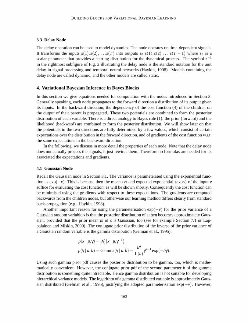
Ghahramani and Roweis have shown (1999) that for the nonlinear function f (s) = exp(−s2) inEq. (7), the mean and variance have analytical expressions, to be presented shortly, provided that ithas Gaussian input. In our graphical network structures this condition is fulfilled if we require thatthe nonlinearity must be inserted immediately after a Gaussian node. The same type of exponentialfunction (7) is frequently used in standard radial-basis function networks (Bishop, 1995; Haykin,1998; Ghahramani and Roweis, 1999), but in a different manner. There the exponential functiondepends on the Euclidean distance from a centre point, while in our case it depends on the inputvariable s directly.
The first and second moments of the function (7) with respect to the distribution q(s) are(Ghahramani and Roweis, 1999)
〈 f (s)〉= exp
(−
s2
2s+1
)(2s+1)−
12 , (25)
⟨[ f (s)]2
⟩= exp
(−
2s2
4s+1
)(4s+1)−
12 . (26)
The formula (25) provides directly the mean 〈 f (s)〉, and the variance is obtained from (25) and(26) by applying the familiar formula Var{ f (s)} =
⟨[ f (s)]2
⟩−〈 f (s)〉2. The expected exponential
〈exp f (s)〉 cannot be evaluated analytically, which limits somewhat the use of the nonlinear node.The updating of the nonlinear node following directly a Gaussian node takes place similarly as
the updating of a plain Gaussian node. The gradients of Cp with respect to 〈 f (s)〉 and Var{ f (s)}are evaluated assuming that they arise from a quadratic term. This assumption holds since thenonlinearity can only propagate to the mean of Gaussian nodes. The update formulas are given inAppendix C.
Another possibility is to use as the nonlinearity the error function f (s) =R s−∞ exp(−r2)dr, be-
cause its mean can be evaluated analytically and variance approximated from above (Frey and Hin-ton, 1999). Increasing the variance increases the value of the cost function, too, and hence it sufficesto minimise the upper bound of the cost function for finding a good solution. Frey and Hinton (1999)apply the error function in MLP (multilayer perceptron) networks (Bishop, 1995; Haykin, 1998) butin a manner different from ours.
Finally, Murphy (1999) has applied the hyperbolic tangent function f (s) = tanh(s), approxi-mating it iteratively with a Gaussian. Honkela and Valpola (2005) approximate the same sigmoidalfunction with a Gauss-Hermite quadrature. This alternative could be considered here, too. A prob-lem with it is, however, that the cost function (mean and variance) cannot be computed analytically.
4.4 Other Possible Nodes
One of the authors has recently implemented two new variable nodes (Harva, 2004; Harva et al.,2005) into the Bayes Blocks software library. They are the mixture-of-Gaussians (MoG) node and
167

RAIKO, VALPOLA, HARVA AND KARHUNEN
Node type 〈·〉 Var{·} 〈exp ·〉
Gaussian node s s (9)Addition node (15) (16) (17)Multiplication node (18) (19) -Nonlinearity (25) (25),(26) -Constant c 0 expc
Table 1: The forward messages or expectations that are provided by the output of different typesof nodes. The numbers in parentheses refer to defining equations. The multiplication andnonlinearity cannot provide the expected exponential.
the rectified Gaussian node. MoG can be used to model any sufficiently well behaving distribution(Bishop, 1995). In the independent factor analysis (IFA) method introduced in Attias (1999), a MoGdistribution was used for the sources, resulting in a probabilistic version of independent componentanalysis (ICA) (Hyvarinen et al., 2001).
The second new node type, the rectified Gaussian variable, was introduced in Miskin andMacKay (2001). By omitting negative values and retaining only positive ones of a variable whichis originally Gaussian distributed, this block allows modelling of variables having positive valuesonly. Such variables are commonplace for example in digital image processing, where the pictureelements (pixels) have always non-negative values. The cost functions and update rules of the MoGand rectified Gaussian node have been derived by Harva (2004). We postpone a more detaileddiscussion of these nodes to forthcoming papers to keep the length of this paper reasonable.
In the early conference paper (Valpola et al., 2001) where we introduced the blocks for thefirst time, two more blocks were proposed for handling discrete models and variables. One ofthem is a switch, which picks up its k-th continuous valued input signal as its output signal. Theother one is a discrete variable k, which has a soft-max prior derived from the continuous valuedinput signals ci of the node. However, we have omitted these two nodes from the present paper,because their performance has not turned out to be adequate. The reason might be that assumingposterior independence of the auxiliary Gaussian variables is too rough and that the cost functionin the soft-max case could not be computed exactly. For instance, building a mixture-of-Gaussiansfrom discrete and Gaussian variables with switches is possible, but the construction loses out to aspecialised MoG node that makes fewer assumptions. Raiko (2005) uses the soft-max node withoutswitches.
Action and utility nodes (Pearl, 1988; Murphy, 2001) would extend the library into decisiontheory and control. In addition to the messages about the variational Bayesian cost function, thenetwork would propagate messages about utility. Raiko and Tornio (2005) describe such a systemin a slightly different framework.
5. Combining the Nodes
The expectations provided by the outputs and required by the inputs of the different nodes aresummarised in Tables 1 and 2, respectively. One can see that the variance input of a Gaussian noderequires the expected exponential of the incoming signal. However, it cannot be computed for thenonlinear and multiplication nodes. Hence all the nodes cannot be combined freely.
168

BUILDING BLOCKS FOR VARIATIONAL BAYESIAN LEARNING
Input type ∂C∂〈·〉
∂C∂Var{·}
∂C∂〈exp ·〉
Mean of a Gaussian node (10) (11) 0Variance of a Gaussian node (12) 0 (13)Addendum (20) (21) (22)Factor (23) (24) 0
Table 2: The backward messages or the gradients of the cost function w.r.t. certain expectations.The numbers in parentheses refer to defining equations. The gradients of the Gaussiannode are derived from Eq. (8). The Gaussian node requires the corresponding expecta-tions from its inputs, that is, 〈m〉, Var{m}, 〈v〉, and 〈expv〉. Addition and multiplicationnodes require the same type of input expectations that they are required to provide asoutput. Communication of a nonlinearity with its Gaussian parent node is described inAppendix C.
When connecting the nodes, the following restrictions must be taken into account:
1. In general, the network has to be a directed acyclic graph (DAG). The delay nodes are anexception because the past values of any node can be the parents of any other nodes. Thisviolation is not a real one in the sense that if the structure were unfolded in time, the resultingnetwork would again be a DAG.
2. The nonlinearity must always be placed immediately after a Gaussian node. This is becausethe output expectations, Equations (25) and (26), can be computed only for Gaussian inputs.The nonlinearity also breaks the general form of the likelihood (14). This is handled by usingspecial update rules for the Gaussian followed by a nonlinearity (Appendix C).
3. The outputs of multiplication and nonlinear nodes cannot be used as variance inputs for theGaussian node. This is because the expected exponential cannot be evaluated for them. Theserestrictions are evident from Tables 1 and 2.
4. There should be only one computational path from a latent variable to a variable. A compu-tational path is a path that consists of computation nodes only. Otherwise, the independencyassumptions used in Equations (8) and (16)–(19) are violated and variational Bayesian learn-ing becomes more complicated (recall Figure 1).
Figure 3 shows examples of model structures that break each of the restrictions in turn. Thesoftware package includes a function that checks whether a given model structure is correct or not.Note that the network may contain loops, that is, the underlying undirected network can be cyclic.Note also that the second, third, and fourth restrictions can be circumvented by inserting mediatingGaussian nodes. A mediating Gaussian node that is used as the variance input of another variable,is called the variance source and it is discussed in the following.
5.1 Nonstationary Variance
In most currently used models, only the means of Gaussian nodes have hierarchical or dynamicalmodels. In many real-world situations the variance is not a constant either but it is more difficult to
169

RAIKO, VALPOLA, HARVA AND KARHUNEN
4.1. 2. 3.Figure 3: Examples of illegal model structures violating each of the restriction described in the text
in turn.
m v m
v s(t) w u(t) s(t)
Figure 4: Left: The Gaussian variable s(t) has a a constant variance exp(−v) and mean m. Right:A variance source is added for providing a non-constant variance input u(t) to the output(source) signal s(t). The variance source u(t) has a prior mean v and prior varianceexp(−w).
model it. For modelling the variance, too, we use the variance source (Valpola et al., 2004) depictedschematically in Figure 4. Variance source is a regular Gaussian node whose output u(t) is used asthe input variance of another Gaussian node. Variance source can convert prediction of the meaninto prediction of the variance, allowing to build hierarchical or dynamical models for the variance.
The output s(t) of a Gaussian node to which the variance source is attached (see the right sub-figure of Fig. 4) has in general a super-Gaussian distribution. Such a distribution is typically charac-terised by long tails and a high peak, and it is formally defined as having a positive value of kurtosis(see Hyvarinen et al. (2001) for a detailed discussion). This property has been proved by Parra et al.(2001) who showed that a nonstationary variance (amplitude) always increases the kurtosis. Theoutput signal s(t) of the stationary Gaussian variance source depicted in the left subfigure of Fig. 4is naturally Gaussian distributed with zero kurtosis. The variance source is useful in modelling nat-ural signals such as speech and images which are typically super-Gaussian, and also in modellingoutliers in the observations.
170

BUILDING BLOCKS FOR VARIATIONAL BAYESIAN LEARNING
Var{u(t)}=0Var{u(t)}=1Var{u(t)}=2
Figure 5: The distribution of s(t) is plotted when s(t)∼N (0,exp[−u(t)]) and u(t)∼N (0, ·). Notethat when Var{u(t)} = 0, the distribution of s(t) is Gaussian. This corresponds to theright subfigure of Fig. 4 when m = v = 0 and exp(−w) = 0,1,2.
5.2 Linear Independent Factor Analysis
In many instances there exist several nodes which have quite similar role in the chosen structure.Assuming that ith such node corresponds to a scalar variable yi, it is convenient to use the vector y =(y1,y2, . . . ,yn)
T to jointly denote all the corresponding scalar variables y1,y2, . . . ,yn. This notationis used in Figures 6 and 7 later on. Hence we represent the scalar source nodes corresponding to thevariables si(t) using the source vector s(t), and the scalar nodes corresponding to the observationsxi(t) using the observation vector x(t).
The addition and multiplication nodes can be used for building an affine transformation
x(t) = As(t)+a+nx(t) (27)
from the Gaussian source nodes s(t) to the Gaussian observation nodes x(t). The vector a denotesthe bias and vector nx(t) denotes the zero-mean Gaussian noise in the Gaussian node x(t). Thismodel corresponds to standard linear factor analysis (FA) assuming that the sources si(t) are mutu-ally uncorrelated; see for example, Hyvarinen et al. (2001).
If instead of Gaussianity it is assumed that each source si(t) has some non-Gaussian prior, themodel (27) describes linear independent factor analysis (IFA). Linear IFA was introduced by Attias(1999), who used variational Bayesian learning for estimating the model except for some partswhich he estimated using the expectation-maximisation (EM) algorithm. Attias used a mixture-of-Gaussians source model, but another option is to use the variance source to achieve a super-Gaussiansource model. Figure 6 depicts the model structures for linear factor analysis and independent factoranalysis.
5.3 A Hierarchical Variance Model
Figure 7 (right subfigure) presents a hierarchical model for the variance, and also shows how itcan be constructed by first learning simpler structures shown in the left and middle subfigures ofFig. 7. This is necessary, because learning a hierarchical model having different types of nodes fromscratch in a completely unsupervised manner would be too demanding a task, ending quite probablyinto an unsatisfactory local minimum.
171

RAIKO, VALPOLA, HARVA AND KARHUNEN
A
u(t) s(t)
x(t)
A
s(t)
x(t)
Figure 6: Model structures for linear factor analysis (FA) (left) and independent factor analysis(IFA) (right).
The final rightmost variance model in Fig. 7 is somewhat involved in that it contains both non-linearities and hierarchical modelling of variances. Before going into its mathematical details andinto the two simpler models in Fig. 7, we point out that we have considered in our earlier papersrelated but simpler block models. In Valpola et al. (2003c), a hierarchical nonlinear model for thedata x(t) is discussed without modelling the variance. Such a model can be applied for example tononlinear ICA or blind source separation. Experimental results (Valpola et al., 2003c) show that thisblock model performs adequately in the nonlinear BSS problem, even though the results are slightlypoorer than for our earlier computationally more demanding model (Lappalainen and Honkela,2000; Valpola et al., 2003b; Honkela and Valpola, 2005) with multiple computational paths.
In another paper (Valpola et al., 2004), we have considered hierarchical modelling of varianceusing the block approach without nonlinearities. Experimental results on biomedical MEG (mag-netoencephalography) data demonstrate the usefulness of hierarchical modelling of variances andexistence of variance sources in real-world data.
Learning starts from the simple structure shown in the left subfigure of Fig. 7. There a variancesource is attached to each Gaussian observation node. The nodes represent vectors, with u1(t) beingthe output vector of the variance source and x(t) the t th observation (data) vector. The vectors u1(t)and x(t) have the same dimension, and each component of the variance vector u1(t) models thevariance of the respective component of the observation vector x(t).
Mathematically, this simple first model obeys the equations
x(t) = a1 +nx(t), (28)
u1(t) = b1 +nu1(t). (29)
Here the vectors a1 and b1 denote the constant means (bias terms) of the data vector x(t) andthe variance variable vector u1(t), respectively. The additive “noise” vector nx(t) determines thevariances of the components of x(t). It has a Gaussian distribution with a zero mean and varianceexp[−u1(t)]:
nx(t)∼N (0,exp[−u1(t)]). (30)
More precisely, the shorthand notation N (0,exp[−u1(t)]) means that each component of nx(t) isGaussian distributed with a zero mean and variance defined by the respective component of thevector exp[−u1(t)]. The exponential function exp(·) is applied separately to each component of the
172

BUILDING BLOCKS FOR VARIATIONAL BAYESIAN LEARNING
A11B
x(t)
x(t)
u (t)
u (t)
u (t) s (t)
1
2 2
1
2
1 1
2
u (t)
B
B A
A
u (t)
2
u (t)
s (t)2
s (t)3
x(t)1
3
Figure 7: Construction of a hierarchical variance model in stages from simpler models. Left: In thebeginning, a variance source is attached to each Gaussian observation node. The nodesrepresent vectors. Middle: A layer of sources with variance sources attached to them isadded. They layers are connected through a nonlinearity and an affine mapping. Right:Another layer is added on the top to form the final hierarchical variance model.
vector −u1(t). Similarly,nu1(t)∼N (0,exp [−v1]) (31)
where the components of the vector v1 define the variances of the zero mean Gaussian variablesnu1(t).
Consider then the intermediate model shown in the middle subfigure of Fig. 7. In this secondlearning stage, a layer of sources with variance sources attached to them is added. These sources arerepresented by the source vector s2(t), and their variances are given by the respective componentsof the variance vector u2(t) quite similarly as in the left subfigure. The (vector) node between thesource vector s2(t) and the variance vector u1(t) represents an affine transformation with a trans-formation matrix A1 including a bias term. Hence the prior mean inputted to the Gaussian variancesource having the output u1(t) is of the form B1f(s2(t))+b1, where b1 is the bias vector, and f(·) isa vector of componentwise nonlinear functions (7). Quite similarly, the vector node between s2(t)and the observation vector x(t) yields as its output the affine transformation A1f(s2(t))+a1, wherea1 is a bias vector. This in turn provides the input prior mean to the Gaussian node modelling theobservation vector x(t).
The mathematical equations corresponding to the model represented graphically in the middlesubfigure of Fig. 7 are:
x(t) = A1f(s2(t))+a1 +nx(t), (32)
u1(t) = B1f(s2(t))+b1 +nu1(t), (33)
s2(t) = a2 +ns2(t), (34)
u2(t) = b2 +nu2(t). (35)
173

RAIKO, VALPOLA, HARVA AND KARHUNEN
Compared with the simplest model (28)–(29), one can observe that the source vector s2(t) of thesecond (upper) layer and the associated variance vector u2(t) are of quite similar form, given in Eqs.(34)–(35). The models (32)–(33) of the data vector x(t) and the associated variance vector u1(t) inthe first (bottom) layer differ from the simple first model (28)–(29) in that they contain additionalterms A1f(s2(t)) and B1f(s2(t)), respectively. In these terms, the nonlinear transformation f(s2(t))of the source vector s2(t) coming from the upper layer have been multiplied by the linear mixingmatrices A1 and B1. All the “noise” terms nx(t), nu1(t), ns2(t), and nu2(t) in Eqs. (32)–(35) aremodelled by similar zero mean Gaussian distributions as in Eqs. (30) and (31).
In the last stage of learning, another layer is added on the top of the network shown in themiddle subfigure of Fig. 7. The resulting structure is shown in the right subfigure. The added newlayer is quite similar as the layer added in the second stage. The prior variances represented bythe vector u3(t) model the source vector s3(t), which is turn affects via the affine transformationB2f(s3(t))+b2 to the mean of the mediating variance node u2(t). The source vector s3(t) providesalso the prior mean of the source s2(t) via the affine transformation A2f(s3(t))+a2.
The model equations (32)–(33) for the data vector x(t) and its associated variance vector u1(t)remain the same as in the intermediate model shown graphically in the middle subfigure of Fig. 7.Note that A1 and B1 are still updated. The model equations of the second and third layer sourcess2(t) and s3(t) as well as their respective variance vectors u2(t) and u3(t) in the rightmost subfigureof Fig. 7 are given by
s2(t) = A2f(s3(t))+a2 +ns2(t),
u2(t) = B2f(s3(t))+b2 +nu2(t),
s3(t) = a3 +ns3(t),
u3(t) = b3 +nu3(t).
Again, the vectors a2, b2, a3, and b3 represent the constant means (biases) in their respective models,and A2 and B2 are mixing matrices with matching dimensions. The vectors ns2(t), nu2(t), ns3(t),and nu3(t) have similar zero mean Gaussian distributions as in Eqs. (30) and (31).
It should be noted that in the resulting network the number of scalar-valued nodes (size of thelayers) can be different for different layers. Additional layers could be appended in the same manner.The final network of the right subfigure in Fig. 7 uses variance nodes in building a hierarchical modelfor both the means and variances. Without the variance sources the model would correspond to anonlinear model with latent variables in the hidden layer. As already mentioned, we have consideredsuch a nonlinear hierarchical model in Valpola et al. (2003c). Note that as latent variables of theupper layer are connected to observations through multiple hidden nodes, having computation nodesas hidden nodes would result in multiple computational paths. This type of structure was used inLappalainen and Honkela (2000), and it has a quadratic computational complexity as opposed tolinear one of the networks in Figure 7.
5.4 Linear Dynamic Models for the Sources and Variances
Sometimes it is useful to complement the linear factor analysis model
x(t) = As(t)+a+nx(t) (36)
with a recursive one-step prediction model for the source vector s(t):
s(t) = Bs(t−1)+b+ns(t). (37)
174
BUILDING BLOCKS FOR VARIATIONAL BAYESIAN LEARNING
−1z
A
B
s(t)
x(t)
−1z
A
B
u(t) s(t)
x(t)
−1z
−1z
A
u(t) s(t)
x(t)
C
Figure 8: Three model structures. A linear Gaussian state-space model (left); the same model com-plemented with a super-Gaussian innovation process for the sources (middle); and a dy-namic model for the variances of the sources which also have a recurrent dynamic model(right).
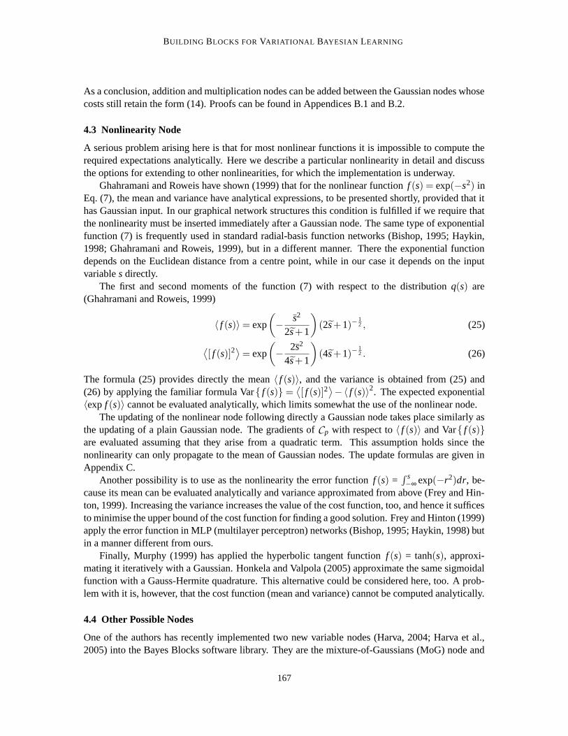
The noise term ns(t) is called the innovation process. The dynamic model of the type (36), (37) isused for example in Kalman filtering (Haykin, 1998, 2001), but other estimation algorithms can beapplied as well (Haykin, 1998). The left subfigure in Fig. 8 depicts the structure arising from Eqs.(36) and (37), built from the blocks.
A straightforward extension is to use variance sources for the sources to make the innovationprocess super-Gaussian. The variance signal u(t) characterises the innovation process of s(t), ineffect telling how much the signal differs from the predicted one but not in which direction it ischanging. The graphical model of this extension is depicted in the middle subfigure of Fig. 8.The mathematical equations describing this model can be written in a similar manner as for thehierarchical variance models in the previous subsection.
Another extension is to model the variance sources dynamically by using one-step recursiveprediction model for them:
u(t) = Cu(t−1)+ c+nu(t).
This model is depicted graphically in the rightmost subfigure of Fig. 8. In context with it, we usethe simplest possible identity dynamical mapping for s(t):
s(t) = s(t−1)+ns(t).
The latter two models introduced in this subsection will be tested experimentally later on in thispaper.
5.5 Hierarchical Priors
It is often desirable that the priors of the parameters should not be too restrictive. A common type ofa vague prior is the hierarchical prior (Gelman et al., 1995). For example the priors of the elements
175

RAIKO, VALPOLA, HARVA AND KARHUNEN
ai j of a mixing matrix A can be defined via the Gaussian distributions
p(ai j | vai ) = N (ai j;0,exp(−va
i )),
p(vai | m
va,vva) = N (vai ;mva,exp(−vva)) .
Finally, the priors of the quantities mva and vva have flat Gaussian distributions N (·;0,100)(the constants depending on the scale of the data). When going up in the hierarchy, we use the samedistribution for each column of a matrix and for each component of a vector. On the top, the numberof required constant priors is small. Thus very little information is provided and needed a priori.This kind of hierarchical priors are used in the experiments later on this paper.
6. Learning
Let us now discuss the overall learning procedure, describing also briefly how problems related withlearning can be handled.
6.1 Updating of the Network
The nodes of the network communicate with their parents and children by providing certain expec-tations in the feedforward direction (from parents to children) and gradients of the cost functionwith respect to the same expectations in the feedback direction (from children to parents). Theseexpectations and gradients are summarised in Tables 1 and 2.
The basic element for updating the network is the update of a single node assuming the restof the network fixed. For computation nodes this is simple: each time when a child node asksfor expectations and they are out of date, the computational node asks from its parents for theirexpectations and updates its own ones. And vice versa: when parents ask for gradients and theyare out of date, the node asks from its children for the gradients and updates its own ones. Theseupdates have analytical formulas given in Section 4.
For a variable node to be updated, the input expectations and output gradients need to be up-to-date. The posterior approximation q(s) can then be adjusted to minimise the cost function asexplained in Section 4. The minimisation is either analytical or iterative, depending on the situation.Signals propagating outwards from the node (the output expectations and the input gradients) of avariable node are functions of q(s) and are thus updated in the process. Each update is guaranteednot to increase the cost function.
One sweep of updating means updating each node once. The order in which this is done is notcritical for the system to work. It would not be useful to update a variable twice without updatingsome of its neighbours in between, but that does not happen with any ordering when updates aredone in sweeps. We have used an ordering where each variable node is updated only after all of itsdescendants have been updated. Basically when a variable node is updated, its input gradients andoutput expectations are labelled as outdated and they are updated only when another node asks forthat information.
It is possible to use different measures to improve the learning process. Measures for avoidinglocal minima are described in the next subsection. Another enhancement can be used for speedingup learning. The basic idea is that after some time, the parameters describing q(s) are changingfairly linearly between consecutive sweeps. Therefore a line search in that direction provides fasterlearning, as discussed in Honkela (2002); Honkela et al. (2003). We apply this line search only atevery tenth sweep for allowing the consecutive updates to become fairly linear again.
176

BUILDING BLOCKS FOR VARIATIONAL BAYESIAN LEARNING
Learning a model typically takes thousands of sweeps before convergence. The cost functiondecreases monotonically after every update. Typically this decrease gets smaller with time, but notalways monotonically. Therefore care should be taken in selecting the stopping criterion. We havechosen to stop the learning process when the decrease in the cost during the previous 200 sweeps islower than some predefined threshold.
6.2 Structural Learning and Local Minima
The chosen model has a pre-specified structure which, however, has some flexibility. The numberof nodes is not fixed in advance, but their optimal number is estimated using variational Bayesianlearning, and unnecessary connections can be pruned away.
A factorial posterior approximation, which is used in this paper, often leads to automatic prun-ing of some of the connections in the model. When there is not enough data to estimate all theparameters, some directions remain ill-determined. This causes the posterior distribution alongthose directions to be roughly equal to the prior distribution. In variational Bayesian learning with afactorial posterior approximation, the ill-determined directions tend to get aligned with the axes ofthe parameter space because then the factorial approximation is most accurate.
The pruning tendency makes it easy to use for instance sparsely connected models, becausethe learning algorithm automatically selects a small amount of well-determined parameters. Butat the early stages of learning, pruning can be harmful, because large parts of the model can getpruned away before a sensible representation has been found. This corresponds to the situationwhere the learning scheme ends up into a local minimum of the cost function (MacKay, 2001). Aposterior approximation which takes into account the posterior dependences has the advantage thatit has far less local minima than a factorial posterior approximation. It seems that Bayesian learningalgorithms which have linear time complexity cannot avoid local minima in general.
However, suitable choices of the model structure and countermeasures included in the learningscheme can alleviate the problem greatly. We have used the following means for avoiding gettingstuck into local minima:
• Learning takes place in several stages, starting from simpler structures which are learned firstbefore proceeding to more complicated hierarchic structures. An example of this techniquewas presented in Section 5.3.
• New parts of the network are initialised appropriately. One can use for instance principalcomponent analysis (PCA), independent component analysis (ICA), vector quantisation, orkernel PCA (Honkela et al., 2004). The best option depends on the application. Often it isuseful to try different methods and select the one providing the smallest value of the costfunction for the learned model. There are two ways to handle initialisation: either to fixthe sources for a while and learn the weights of the model, or to fix the weights for a whileand learn the sources corresponding to the observations. The fixed variables can be releasedgradually (Valpola et al., 2003c, Section 5.1).
• Automatic pruning is discouraged initially by omitting the term
2Var{s2}∂C
∂Var{s1s2}〈s1〉
177
RAIKO, VALPOLA, HARVA AND KARHUNEN
in the multiplication nodes (Eq. (23)). This effectively means that the mean of s1 is optimisti-cally adjusted as if there were no uncertainty about s2. In this way the cost function mayincrease at first due to overoptimism, but it may pay off later on by escaping early pruning.
• New sources si(t) (components of the source vector s(t) of a layer) are generated, and prunedsources are removed from time to time.
• The activations of the sources are reset a few times. The sources are re-adjusted to their placeswhile keeping the mapping and other parameters fixed. This often helps if some of the sourcesare stuck into a local minimum.
7. Experimental Results
The Bayes Blocks software (Valpola et al., 2003a) has been applied to several problems.
Valpola et al. (2004) considered several models of variance. The main application was theanalysis of MEG measurements from a human brain. In addition to features corresponding to brainactivity the data contained several artifacts such as muscle activity induced by the patient bitinghis teeth. Linear ICA applied to the data was able to separate the original causes to some degreebut still many dependencies remained between the sources. Hence an additional layer of so-calledvariance sources was used to find correlations between the variances of the innovation processes ofthe ordinary sources. These were able to capture phenomena related to the biting artifact as well asto rhythmic activity.
An astrophysical problem of separating young and old star populations from a set of ellipticalgalaxy spectra was studied by one of the authors in Nolan et al. (2006). Since the observed quantitieswere energies and thus positive and since the mixing process was also known to be positive, it wasnecessary for the subsequent astrophysical analysis to be feasible to include these constraints tothe model as well. The standard technique of putting a positive prior on the sources was foundto have the unfortunate technical shortcoming of inducing sparsely distributed factors, which wasdeemed inappropriate in that specific application. To get rid of the induced sparsity but to stillkeep the positivity constraint, the nonnegativity was forced by rectification nonlinearities (Harvaand Kaban, 2007). In addition to finding an astrophysically meaningful factorisation, several otherspecifications were needed to be met related to handling of missing values, measurements errorsand predictive capabilities of the model.
In Raiko (2005), a nonlinear model for relational data was applied to the analysis of the boardgame Go. The difficult part of the game state evaluation is to determine which groups of stones arelikely to get captured. A model similar to the one that will be described in Section 7.2, was built forfeatures of pairs of groups, including the probability of getting captured. When a learned model isapplied to new game states, the estimates propagate through a network of such pairs. The structureof the network is thus determined by the game state. The approach can be used for inference inrelational databases.
The following three sets of experiments are given as additional examples. The first one is adifficult toy problem that illustrates hierarchy and variance modelling, the second one studies theinference of missing values in speech spectra, and the third one has a dynamical model for imagesequences.
178

BUILDING BLOCKS FOR VARIATIONAL BAYESIAN LEARNING
Figure 9: Samples from the 1000 image patches used in the extended bars problem. The barsinclude both standard and variance bars in horizontal and vertical directions. For instance,the patch at the bottom left corner shows the activation of a standard horizontal bar abovethe horizontal variance bar in the middle.
7.1 Bars Problem
The first experimental problem studied was testing of the hierarchical nonlinear variance model inFigure 7 in an extension of the well-known bars problem (Dayan and Zemel, 1995). The data setconsisted of 1000 image patches each having 6× 6 pixels. They contained both horizontal andvertical bars. In addition to the regular bars, the problem was extended to include horizontal andvertical variance bars, characterised and manifested by their higher variance. Samples of the imagepatches used are shown in Figure 9.
The data were generated by first choosing whether vertical, horizontal, both, or neither orienta-tions were active, each with probability 1/4. Whenever an orientation is active, there is a probability1/3 for a bar in each row or column to be active. For both orientations, there are 6 regular bars, onefor each row or column, and 3 variance bars which are 2 rows or columns wide. The intensities (greylevel values) of the bars were drawn from a normalised positive exponential distribution having thepdf p(z) = exp(−z),z ≥ 0, p(z) = 0,z < 0. Regular bars are additive, and variance bars produceadditive Gaussian noise having the standard deviation of its intensity. Finally, Gaussian noise witha standard deviation 0.1 was added to each pixel.
The network was built up following the stages shown in Figure 7. It was initialised with a singlelayer with 36 nodes corresponding to the 36 dimensional data vector. The second layer of 30 nodeswas created at the sweep 20, and the third layer of 5 nodes at the sweep 100. After creating a layeronly its sources were updated for 10 sweeps, and pruning was discouraged for 50 sweeps. Newnodes were added twice, 3 to the second layer and 2 to the third layer, at sweeps 300 and 400.After that, only the sources were updated for 5 sweeps, and pruning was again discouraged for 50sweeps. The source activations were reset at the sweeps 500, 600 and 700, and only the sourceswere updated for the next 40 sweeps. Dead nodes were removed every 20 sweeps. The multistagetraining procedure was designed to avoid suboptimal local solutions, as discussed in Section 6.2.Note that a large part of the presented procedure could be automated for application to any problem.
Figure 10 demonstrates that the algorithm finds a generative model that is quite similar to thegeneration process. The two sources on the third layer correspond to the horizontal and verticalorientations and the 18 sources on the second layer correspond to the bars. Each element of the
179

RAIKO, VALPOLA, HARVA AND KARHUNEN
weight matrices is depicted as a pixel with the appropriate grey level value in Fig. 10. The pixelsof A2 and B2 are ordered similarly as the patches of A1 and B1, that is, vertical bars on the leftand horizontal bars on the right. Regular bars, present in the mixing matrix A1, are reconstructedaccurately, but the variance bars in the mixing matrix B1 exhibit some noise. The grouping ofhorizontal and vertical orientations is clearly visible in the mixing matrix A2. For instance, the firstpatch in A2 has non-zero (black) weights to all the vertical features, that is, left side pixels in A2
activate sources corresponding to the left side patches in A1 and B1.
A2 (18×2) B2 (18×2)
A1 (36×18) B1 (36×18)
Figure 10: Results of the extended bars problem: Posterior means of the weight matrices afterlearning. The sources of the second layer have been ordered for visualisation purposesaccording to the weight (mixing) matrices A2 and B2. The elements of the matriceshave been depicted as pixels having corresponding grey level values. The 18 pixels inthe weight matrices A2 and B2 correspond to the 18 patches in the weight matrices A1
and B1.
A comparison experiment with a simplified learning procedure was run to demonstrate the im-portance of local optima. The creation and pruning of layers were done as before, but other methodsfor avoiding local minima (addition of nodes, discouraging pruning and resetting of sources) weredisabled. The resulting weights can be seen in Figure 11. This time the learning ends up in a subop-timal local optimum of the cost function. One of the bars was not found (second horizontal bar fromthe bottom), some were mixed up in a same source (most variance bars share a source with a regularbar), fourth vertical bar from the left appears twice, and one of the sources just suppresses varianceeverywhere. The resulting cost function (4) is worse by 5292 compared to the main experiment.The ratio of the model evidences is thus roughly exp(5292).
Figure 12 illustrates the formation of the posterior distribution of a typical single variable. It isthe first component of the variance source u1(1) in the comparison experiment. The prior meanshere the distribution given its parents (especially s2(1) and B1) and the likelihood means the po-
180

BUILDING BLOCKS FOR VARIATIONAL BAYESIAN LEARNING
0 500 1000 15001
1.5
2
2.5
3
3.5
4x 10
4 A2 (14×2) B2 (14×2)
A1 (36×14) B1 (36×14)
Figure 11: Left: Cost function plotted against the number of learning sweeps. Solid curve is themain experiment and the dashed curve is the comparison experiment. The peaks appearwhen nodes are added. Right: The resulting weights in the comparison experiment areplotted like in Figure 10.
priorlikelihoodposteriorapproximation
Figure 12: A typical example illustrating the posterior approximation of a variance source.
tential given its children (the first component of x(1)). Assuming the posteriors of other variablesaccurate, we can plot the true posterior of this variable and compare it to the Gaussian posteriorapproximation. Their difference is only 0.007 measured by Kullback-Leibler divergence.
7.2 Missing Values in Speech Spectra
In hierarchical nonlinear factor analysis (HNFA) (Valpola et al., 2003c), there are a number of layersof Gaussian variables, the bottom-most layer corresponding to the data. There is a nonlinearity anda linear mixture mapping from each layer to all the layers below it.
HNFA resembles the model structure in Section 5.3. The model structure is depicted in the leftsubfigure of Fig. 13. Model equations are
h(t) = As(t)+a+nh(t),
x(t) = Bφ[h(t)]+Cs(t)+b+nx(t) ,
181

RAIKO, VALPOLA, HARVA AND KARHUNEN
s(t)
x(t)
h(t)
C
A
B
Generalisation4.
2.1.
3.
dimensionalityHigh
Memorisation(permuted)
Nonlinearity(patches)
Figure 13: Left: The model structure for hierarchical nonlinear factor analysis (HNFA). Right: Fourdifferent experimental settings with the speech data used for measuring different prop-erties of the algorithms.
where nh(t) and nx(t) are Gaussian noise terms and the nonlinearity φ(ξ) = exp(−ξ2) again operateson each element of its argument vector separately. Note that we have included a short-cut mappingC from sources to observations. This means that hidden nodes only need to model the deviationsfrom linearity.
HNFA is compared against three other methods. Factor analysis (FA) is a linear method de-scribed in Section 5.2. It is a special case of HNFA where the dimensionality of h(t) is zero. Non-linear factor analysis (NFA) (Lappalainen and Honkela, 2000; Honkela and Valpola, 2005) differsfrom HNFA in that it does not use mediating variables h(t):
x(t) = B tanh[As(t)+a]+b+nx(t).
Note that NFA has multiple computational paths between s(t) and x(t), which leads to a highercomputational complexity compared to HNFA.
The self-organising map SOM (Kohonen, 2001) differs most from the other methods. A rect-angular map has a number of map units with associated model vectors that are points in the dataspace. Each data point is matched to the closest map unit. The model vectors of the best-matchingunit and its neighbours in the map are moved slightly towards the data point. See Kohonen (2001);Haykin (1998) for details.
The data set consisted of speech spectrograms from several Finnish subjects. Short term spec-tra were acquired by using Fourier transformation and their dimensionality was reduced to 30 bytriangular windowing with window centres uniformly spaced on the Mel scale. It is clear that adynamic source model would give better reconstructions, but in this case the temporal informationwas left out to ease the comparison of the models. Half of the about 5000 samples were used as test
182

BUILDING BLOCKS FOR VARIATIONAL BAYESIAN LEARNING
Data with missing values Original data
HNFA reconstruction NFA reconstruction
FA reconstruction SOM reconstruction
Figure 14: Some speech data with and without missing values (Setting 1) and reconstructions byHNFA and by comparison models.
data with some missing values. Missing values were set in four different ways to measure differentproperties of the algorithms (right subfigure of Fig. 13):
1. 38 percent of the values are set to miss randomly in 4×4 patches. (Figure 14)
2. The data samples are randomly permuted before setting missing values in 4×4 patches as inSetting 1.
3. 10 percent of the values are set to miss randomly independent of any neighbours. This is aneasier setting, since simple smoothing using nearby values would give fine reconstructions.
4. The data samples are permuted and 10 percent of the values are set to miss independently ofany neighbours.
With permutation, data samples from a single spoken word end up in both training and testing data.This setting emphasises memorisation, while testing with new speech emphasises generalisation.When values are missing one by one, they could be reconstructed quite well even by linear inter-polation of their neighbours. Thus, this setting emphasises the models ability to work accurately inhigh dimensions rather than its capability of modelling nonlinear effects.
We tried to optimise each method and in the following, we describe how we got the best results.The self-organising map was run using the SOM Toolbox (Vesanto et al., 1999) with long learningtime, 2500 map units and random initialisations. In other methods, the optimisation was based onminimising the cost function or its approximation. NFA was learned for 5000 sweeps through datausing a Matlab implementation. Varying number of sources were tried out and the best ones wereused as the result. The optimal number of sources was around 12 to 15 and the size used for thehidden layer was 30. A large enough number should do, since the algorithm can effectively pruneout parts that are not needed.
In factor analysis (FA), the number of sources was 28. In hierarchical nonlinear factor analysis(HNFA), the number of sources at the top layer was varied and the best runs according to the cost
183
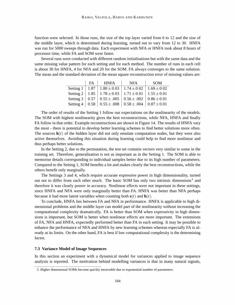
RAIKO, VALPOLA, HARVA AND KARHUNEN
function were selected. In those runs, the size of the top layer varied from 6 to 12 and the size ofthe middle layer, which is determined during learning, turned out to vary from 12 to 30. HNFAwas run for 5000 sweeps through data. Each experiment with NFA or HNFA took about 8 hours ofprocessor time, while FA and SOM were faster.
Several runs were conducted with different random initialisations but with the same data and thesame missing value pattern for each setting and for each method. The number of runs in each cellis about 30 for HNFA, 4 for NFA and 20 for the SOM. FA always converges to the same solution.The mean and the standard deviation of the mean square reconstruction error of missing values are:
FA HNFA NFA SOMSetting 1 1.87 1.80±0.03 1.74±0.02 1.69±0.02Setting 2 1.85 1.78±0.03 1.71±0.01 1.55±0.01Setting 3 0.57 0.55± .005 0.56± .002 0.86±0.01Setting 4 0.58 0.55± .008 0.58± .004 0.87±0.01
The order of results of the Setting 1 follow our expectations on the nonlinearity of the models.The SOM with highest nonlinearity gives the best reconstructions, while NFA, HNFA and finallyFA follow in that order. Example reconstructions are shown in Figure 14. The results of HNFA varythe most - there is potential to develop better learning schemes to find better solutions more often.The sources h(t) of the hidden layer did not only emulate computation nodes, but they were alsoactive themselves. Avoiding this situation during learning could help to find more nonlinear andthus perhaps better solutions.
In the Setting 2, due to the permutation, the test set contains vectors very similar to some in thetraining set. Therefore, generalisation is not as important as in the Setting 1. The SOM is able tomemorise details corresponding to individual samples better due to its high number of parameters.Compared to the Setting 1, SOM benefits a lot and makes clearly the best reconstructions, while theothers benefit only marginally.
The Settings 3 and 4, which require accurate expressive power in high dimensionality, turnedout not to differ from each other much. The basic SOM has only two intrinsic dimensions3 andtherefore it was clearly poorer in accuracy. Nonlinear effects were not important in these settings,since HNFA and NFA were only marginally better than FA. HNFA was better than NFA perhapsbecause it had more latent variables when counting both s(t) and h(t).
To conclude, HNFA lies between FA and NFA in performance. HNFA is applicable to high di-mensional problems and the middle layer can model part of the nonlinearity without increasing thecomputational complexity dramatically. FA is better than SOM when expressivity in high dimen-sions is important, but SOM is better when nonlinear effects are more important. The extensionsof FA, NFA and HNFA, expectedly performed better than FA in each setting. It may be possible toenhance the performance of NFA and HNFA by new learning schemes whereas especially FA is al-ready at its limits. On the other hand, FA is best if low computational complexity is the determiningfactor.
7.3 Variance Model of Image Sequences
In this section an experiment with a dynamical model for variances applied to image sequenceanalysis is reported. The motivation behind modelling variances is that in many natural signals,
3. Higher dimensional SOMs become quickly intractable due to exponential number of parameters.
184

BUILDING BLOCKS FOR VARIATIONAL BAYESIAN LEARNING
there exists higher order dependencies which are well characterised by correlated variances of thesignals (Parra et al., 2001). Hence we postulate that we should be able to better catch the dynamicsof a video sequence by modelling the variances of the features instead of the features themselves.This indeed is the case as will be shown.
The model considered can be summarised by the following set of equations:
x(t)∼N (As(t),diag(exp[−vx])),
s(t)∼N (s(t−1),diag(exp[−u(t)])),
u(t)∼N (Bu(t−1),diag(exp[−vu])).
We will use the acronym DynVar in referring to this model. The linear mapping A from sourcess(t) to observations x(t) is constrained to be sparse by assigning each source a circular region on theimage patch outside of which no connections are allowed. These regions are still highly overlapping.The variances u(t) of the innovation process of the sources have a linear dynamical model. It shouldbe noted that modelling the variances of the sources in this manner is impossible if one is restrictedto use conjugate priors.
The sparsity of A is crucial as the computational complexity of the learning algorithm dependson the number of connections from s(t) to x(t). The same goal could have been reached with adifferent kind of approach as well. Instead of constraining the mapping to be sparse from the verybeginning of learning it could have been allowed to be full for a number of iterations and onlyafter that pruned based on the cost function as explained in Section 6.2. But as the basis for imagesequences tends to get sparse anyway, it is a waste of computational resources to wait while mostof the weights in the linear mapping tend to zero.
For comparison purposes, we postulate another model where the dynamical relations are soughtdirectly between the sources leading to the following model equations:
x(t)∼N (As(t),diag(exp[−vx])),
s(t)∼N (Bs(t−1),diag(exp[−vs])).
We shall refer to this model as DynSrc.The data x(t) was a video image sequence (van Hateren and Ruderman, 1998) of dimensions
16×16×4000. That is, the data consisted of 4000 subsequent digital images of the size 16×16. Apart of the data set is shown in Figure 15.
Both models were learned by iterating the learning algorithm 2000 times at which stage a suffi-cient convergence was attained. The first hint of the superiority of the DynVar model was providedby the difference of the cost between the models which was 28 bits/frame (for the coding inter-pretation, see Honkela and Valpola, 2004). To further evaluate the performance of the models,we considered a simple prediction task where the next frame was predicted based on the previousones. The predictive distributions, p(x(t + 1)|x(1), ...,x(t)), for the models can be approximatelycomputed based on the posterior approximation. The means of the predictive distributions are verysimilar for both of the models. Figure 16 shows the means of the DynVar model for the same se-quence as in Figure 15. The means themselves are not very interesting, since they mainly reflectthe situation in the previous frame. However, the DynVar model provides also a rich model forthe variances. The standard deviations of its predictive distribution are shown in Figure 17. Whitestands for a large variance and black for a small one. Clearly, the model is able to increase thepredicted variance in the area of high motion activity and hence provide better predictions. We can
185

RAIKO, VALPOLA, HARVA AND KARHUNEN
offer quantitative support for this claim by computing the predictive perplexities for the models.Predictive perplexity is widely used in language modelling and it is defined as
perplexity(t) = exp
{−
1256
256
∑i=1
log p(xi(t +1)|x(1), ...,x(t))
}.
The predictive perplexities for the same sequence as in Figure 15 are shown in Figure 18. Naturallythe predictions get worse when there is movement in the video. However, DynVar model is able tohandle it much better than the compared DynSrc model. The same difference can also be directlyread by comparing the cost functions (2).
The possible applications for a model of image sequences include video compression, motiondetection, early stages of computer vision, and making hypotheses on biological vision.
8. Discussion
One of the distinctive factors between different Bayesian approaches is the type of posterior approx-imation. We have concentrated on large unsupervised learning tasks, where point estimates are tooprone to overfitting and sampling used in MCMC methods and particle filters, is often too slow. Theproblems tackled with particle filters in Doucet et al. (2001) vary from 1 to 10 in dimensionality,whereas the latent space in Section 7.3 is 128 dimensional. The variational Bayesian learning seemsto provide a good compromise between point estimates and sampling methods.
Often the posterior distribution consists of clusters or solution modes. It depends on the pos-terior approximation again, whether only one of the clusters, or all of them are modelled. In ourcase, the expectation in JKL(q ‖ p) is taken over the approximate distribution q, which in practiceleads to modelling a single mode. In expectation propagation (Minka, 2001), the Kullback-Leiblerdivergence is formed differently, leading to modelling of all the modes. Also, sampling is supposedto take place in all the modes. For the purpose of finding a single good representative of the pos-terior probability mass, the first approach should be better. In fact, the expectation over the trueposterior, also known as the Bayes estimate, is often degenerate due to symmetry. For instance infactor analysis type models, the posterior is symmetric to the permutation of factors. The numberof permutations also gives a hint of the infeasibility of accurately modelling all the modes in a high-dimensional problem. Perhaps it would be best to find one mode for the parameters, but all modesfor the time-dependent variables when feasible.
The variational Bayesian methods vary further depending on the posterior approximation. Inthis paper, all variables are assumed to be independent a posteriori. We have chosen to modelindividual distributions as Gaussians. Often different conjugate distributions are used instead, forinstance, the variance of a Gaussian variable is modelled with a Gamma distribution. Conjugatedistributions are accurate and in some sense practical, but by restricting to Gaussians, the nodes canbe connected more freely allowing for example hierarchical modelling of variances. It should benoted that the effect of assuming independencies is far more significant compared to the effect ofapproximations in modelling individual distributions.
The scope of this paper has been restricted to models which can be learned using purely localcomputations. This is possible, if the parents of each node are independent a posteriori. This canbe accomplished by using a factorial posterior approximation and by not allowing multiple compu-tational paths between variables. Purely local computations result in a computational complexitythat is linear w.r.t. the number of connections in the model. In small models, one could afford to
186

BUILDING BLOCKS FOR VARIATIONAL BAYESIAN LEARNING
Figure 15: A sequence of 80 frames from the data used in the experiment.
Figure 16: The means of the predictive distribution for the DynVar model.
187

RAIKO, VALPOLA, HARVA AND KARHUNEN
Figure 17: The standard deviations of the predictive distribution for the DynVar model.
0 10 20 30 40 50 60 70 800
5
10
15
20
25
Frame
Pre
d. P
erpl
exity
DynSrcDynVar
Figure 18: Predictive perplexities. Perplexity means that the model is as perplexed as if it werechoosing between perplexity(t) equally likely options. Low perplexity means high com-pression.
188

BUILDING BLOCKS FOR VARIATIONAL BAYESIAN LEARNING
take all the dependencies into account. In larger models, it might be desirable to model posteriordependencies within disjoint groups of variables, but to assume the groups statistically independent,as is done by Winn and Bishop (2005).
According to our experience, almost maximally factorial posterior pdf approximation q(θ) suf-fices in many cases. It seems that a good model structure is usually more important than a goodapproximation of the posterior pdf of the model. Therefore the available computation time is of-ten better invested in a larger model using a simple posterior approximation. In any case, densityestimates of continuous valued latent variables offer an important advantage over point estimates,because they are robust against overfitting and provide a cost function suitable for learning modelstructures. With variational Bayesian learning employing a factorial posterior pdf approximationq(θ) the density estimates are almost as efficient as point estimates. Moreover, latent variable mod-els often exhibit rotational and other invariances of which variational Bayesian learning can takeadvantage by choosing a solution where the factorial approximation is most accurate.
The basic algorithm for learning and inference is based on updating a variable at a time whilekeeping other variables fixed. It has the benefits of being completely local and guaranteed to con-verge. A drawback is that the flow of information through time can be slow while performinginference in a dynamical model. There are alternative inference algorithms, where updates are car-ried out in forward and backward sweeps. These include particle smoothing (Doucet et al., 2001),extended Kalman smoothing (Anderson and Moore, 1979), and expectation propagation (Minka,2001). Raiko et al. (2006) propose an algorithm that combines guaranteed convergence with fasterflow of information in variational Bayesian inference that could be applied here as well. Whenthe model needs to be learned at the same time, one needs to iterate a lot anyway, so the varia-tional Bayesian algorithm that makes small but consistent improvements at every sweep might bepreferable.
It is an important design choice that each node is updated while keeping the other nodes fixed.If new node types are added later on, there is no need to change the global learning algorithm, butit suffices to design an update rule for the new node type. Also, there is an option to update somenodes more often than others. When different parameters are coupled and cyclic updating is slow,it can be sped up by line search as described by Honkela et al. (2003). Note that all the updatesare done in order to minimise a global cost function, that is, a cost function over all the variables.Expectation propagation (Minka, 2001) updates one approximation at a time, too. An importantdifference is that there updates are done using a local cost function, that is, the local approximationis fitted to the local true posterior assuming that the rest of the approximation is accurate. This isthe reason why expectation propagation may diverge.
Large nonlinear problems often have numerous suboptimal local solutions that should be avoided.We have used many tricks to avoid them, as discussed in Section 6.2. It depends on the applicationwhich tricks work best. It is an important aspect of future work to make the procedure as simple aspossible for the user.
9. Conclusions
In this paper, we have introduced standardised nodes (blocks) for constructing generative latentvariable models. These nodes include a Gaussian node, addition, multiplication, a nonlinearityfollowing directly a Gaussian node, and a delay node. The nodes have been designed so that theyfit together, allowing construction of many types of latent variable models, including both known
189

RAIKO, VALPOLA, HARVA AND KARHUNEN
and novel structures. Constructing new prototype models is rapid since the user does not need totake care of the learning formulas. The nodes have been implemented in an open source softwarepackage called the Bayes Blocks (Valpola et al., 2003a).
The models built from these blocks are taught using variational Bayesian (ensemble) learning.This learning method essentially uses as its cost function the Kullback-Leibler information betweenthe true posterior density and its approximation. The cost function is used for updating the un-known variables in the model, but it also allows optimisation of the number of nodes in the chosenmodel type. By using a factorial posterior density approximation, all the required computations canbe carried out locally by propagating means, variances, and expected exponentials instead of fulldistributions. In this way, one can achieve a linear computational complexity with respect to thenumber of connections in the chosen model. However, initialisation to avoid premature pruning ofnodes and local minima require special attention in each application for achieving good results.
In this paper, we have tested the introduced method experimentally in three separate unsuper-vised learning problems with different types of models. The results demonstrate the good perfor-mance and usefulness of the method. First, hierarchical nonlinear factor analysis (HNFA) withvariance modelling was applied to an extension of the bars problem. The presented algorithm couldfind a model that is essentially the same as the complicated way in which the data were generated.Secondly, HNFA was used to reconstruct missing values in speech spectra. The results were con-sistently better than with linear factor analysis, and were generally best in cases requiring accuraterepresentation in high dimensionality. The third experiment was carried out using real-world videoimage data. We compared the linear dynamical model for the means and for the variances of thesources. The results demonstrate that finding strong dependencies between different sources wasconsiderably easier when the variances were modelled, too.
Acknowledgments
We thank Antti Honkela, Tomas Ostman, and Alexander Ilin for work on Bayes blocks softwarelibrary and for useful comments, and Hans van Hateren for supplying the video data (van Haterenand Ruderman, 1998) used in the experiments. This research has been funded by the EuropeanCommission project BLISS and the Finnish Centre of Excellence Programme (2000-2005) underthe project New Information Processing Principles.
Appendix A. Updating q(s) for the Gaussian Node
Here we show how to minimise the function
C (m,v) = Mm+V [(m−m0)2 + v]+E exp(m+ v/2)−
12
lnv,
where M,V ,E, and m0 are scalar constants. A unique solution exists when V > 0 and E ≥ 0. Thisproblem occurs when a Gaussian posterior with mean m and variance v is fitted to a probabilitydistribution whose logarithm has both a quadratic and exponential part resulting from Gaussian priorand log-Gamma likelihoods, respectively, and Kullback-Leibler divergence is used as the measureof the misfit.
In the special case E = 0, the minimum of C (m,v) can be found analytically and it is m =m0 −
M2V , v = 1
2V . In other cases where E > 0, minimisation is performed iteratively. At each
190

BUILDING BLOCKS FOR VARIATIONAL BAYESIAN LEARNING
iteration, one Newton iteration for the mean m and one fixed-point iteration for the variance v arecarried out as explained in more detail in the following.
A.1 Newton Iteration for the Mean m
The Newton iteration for m is obtained by
mi+1 = mi−∂C (mi,vi)/∂mi
∂2C (mi,vi)/∂m2i
= mi−M +2V (mi−m0)+E exp(m+ v/2)
2V +E exp(m+ v/2). (38)
The Newton iteration converges in one step if the second derivative remains constant. The step istoo short if the second derivative decreases and too long if the second derivative increases. Forstability, it is better to take too short than too long steps.
In this case, the second derivative always decreases if the mean m decreases and vice versa. Forstability it is therefore useful to restrict the growth of m because it is consistently over-estimated.
A.2 Fixed-Point Iteration for the Variance v
A simple fixed-point iteration rule is obtained for the variance v by solving the zero of the derivative:
0 =∂C (m,v)
∂v= V +
E2
exp(m+ v/2)−12v⇔
v =1
2V +E exp(m+ v/2)
def= g(v),
vi+1 = g(vi). (39)
In general, fixed-point iterations are stable around the solution vopt if |g′(vopt)| < 1 and convergebest when the derivative g′(vopt) is near zero. In our case g′(vi) is always negative and can be lessthan −1. In this case the solution can be an unstable fixed-point. This can be avoided by taking aweighted average of (39) and a trivial iteration vi+1 = vi:
vi+1 =ξ(vi)g(vi)+ vi
ξ(vi)+1def= f (vi). (40)
The weight ξ should be such that the derivative of f is close to zero at the optimal solution vopt
which is achieved exactly when ξ(vopt) =−g′(vopt).It holds
g′(v) =−(E/2)exp(m+ v/2)
[2V +E exp(m+ v/2)]2= g2(v)
[V −
12g(v)
]= g(v)
[V g(v)−
12
]⇒
g′(vopt) = vopt
[V vopt−
12
]⇒ ξ(vopt) = vopt
[12−V vopt
].
The last steps follow from the fact that vopt = g(vopt) and from the requirement that f ′(vopt) = 0. Wecan assume that v is close to vopt and use
ξ(v) = v
[12−V vopt
]. (41)
191

RAIKO, VALPOLA, HARVA AND KARHUNEN
Note that the iteration (39) can only yield estimates with 0 < vi+1 < 1/2V which means thatξ(vi+1) > 0. Therefore the use of ξ always shortens the step taken in (40). If the initial estimatev0 > 1/2V , we can set it to v0 = 1/2V .
There is potential for a speedup by doing a joint Newton’s iteration on both m and v at the sametime. Another option would be to allow m to be updated more often than v.
A.3 Summary of the Updating Method for q(s)
1. Set v0←min(v0,1/2V ).
2. Iterate:
(a) Solve the new estimate of the mean m from Eq. (38) under the restriction that the maxi-mum step is 4;
(b) Solve the new estimate of the variance v from Eqs. (41) and (40) under the restrictionthat the maximum step is 4.
3. Stop the iteration after the corrections become small enough, being under some suitable pre-defined threshold value.
Appendix B. Addition and Multiplication Nodes
Equations (15)–(19) for the addition and multiplication nodes are proven in the following section.Only the Equation (15) applies in general, the others assume that the incoming signals are inde-pendent a posteriori. That is, q(s1,s2, . . . ,sn) = q(s1)q(s2) . . .q(sn). Also the proof of the form ofthe cost function mostly concerns propagation through addition and multiplication nodes, so it ispresented here. Finally, the formulas of propagating the gradients of the cost function w.r.t. theexpectations are derived.
B.1 Expectations
Equation (15) follows directly from the linearity of the expectation operation, or can be provenanalogously to the proof of Equation (18):
⟨n
∏i=1
si
⟩=
Z
(n
∏i=1
si
)q(s1,s2, . . . ,sn)ds
=Z n
∏i=1
siq(si)ds =n
∏i=1
Z
siq(si)dsi =n
∏i=1
〈si〉 .
Equation (16) states that the variance of a sum of independent variables is the sum of theirvariances. This fact can be found in basic probability theory books. It can be proven with simplemanipulation by using Equations (15) and (18).
Equation (17) can be proven by applying (18) to expsi:
⟨exp
(n
∑i=1
si
)⟩=
⟨n
∏i=1
expsi
⟩=
n
∏i=1
〈expsi〉 .
192

BUILDING BLOCKS FOR VARIATIONAL BAYESIAN LEARNING
Equation (19) can be proven by applying Equation (18) to both si and s2i :
Var
{n
∏i=1
si
}=
⟨(n
∏i=1
si
)2⟩−
⟨n
∏j=1
s j
⟩2
=
⟨n
∏i=1
s2i
⟩−
(n
∏j=1
⟨s j⟩)2
=n
∏i=1
⟨s2
i
⟩−
n
∏j=1
⟨s j⟩2
=n
∏i=1
[〈si〉
2 +Var{si}]−
n
∏j=1
⟨s j⟩2
.
B.2 Form of the Cost Function
The form of the part of the cost function that an output of a node affects is shown to be of the form
Cp = M 〈·〉+V [(〈·〉−〈·〉current)2 +Var{·}]+E 〈exp ·〉+C. (42)
where 〈·〉 denotes the expectation of the quantity in question. If the output is connected directly toanother variable, this can be seen from Eq. (8) by substituting
M = 〈expv〉(〈s〉current−〈m〉),
V =12〈expv〉 ,
E = 0,
C =12
[〈expv〉
(Var{m}+ 〈m〉2−〈s〉2current
)−〈v〉+ ln2π
].
If the output is connected to multiple variables, the sum of the affected costs is of the same form.Now one has to prove that this form remains the same when the signals are fed through the additionand multiplication nodes.4
If the cost function is of the predefined form (42) for the sum s1 + s2, it has the same form fors1, when s2 is regarded as a constant. This can be shown using Eqs. (15), (16), and (17):
Cp = M 〈s1 + s2〉+V[(〈s1 + s2〉−〈s1 + s2〉current)
2 +Var{s1 + s2}]
+E 〈exp(s1 + s2)〉+C (43)
= M 〈s1〉+V[(〈s1〉−〈s1〉current)
2 +Var{s1}]
+(E 〈exps2〉)〈exps1〉+(C +M 〈s2〉+V Var{s2}) .
It can also be seen from (43) that when E = 0 for the sum s1 + s2, it is zero for the addend s1, that isE ′ = E 〈exps2〉= 0. This means that the outputs of product and nonlinear nodes can be fed throughaddition nodes.
If the cost function is of the predefined form (42) with E = 0 for the product s1s2, it is similarfor the variable s1, when the variable s2 is regarded as a constant. This can be shown using Eqs. (18)
4. Note that delay node only rewires connections so it does not affect the formulas.
193

RAIKO, VALPOLA, HARVA AND KARHUNEN
and (19):
Cp = M 〈s1s2〉+V[(〈s1s2〉−〈s1s2〉current)
2 +Var{s1s2}]+C
= (M 〈s2〉+2V Var{s2}〈s1〉current)〈s1〉
+[V(〈s2〉
2 +Var{s2})][
(〈s1〉−〈s1〉current)2 +Var{s1}
]
+(
C−V Var{s2}〈s1〉2current
).
Appendix C. Updating q(s) for the Gaussian Node Followed by a Nonlinearity
A Gaussian variable has its own terms in the cost function and it affects the cost function of itschildren. In case there is a nonlinearity attached to it, only the latter is changed. The cost functionof the children can be written in the form
Cch(s),p = M 〈 f (s)〉+V [(〈 f (s)〉−〈 f (s)〉current)2 +Var{ f (s)}]
where 〈 f (s)〉current stands for the expectation using the current posterior estimate q(s), and M and Vare constants.
The posterior q(s) = N (s;s, s) is updated to minimise the cost function. For s we get a fixedpoint iteration for the update candidate:
snew =
[〈expv〉+
4V(1−2s2 +2s
)(〈 f (s)〉− M
2V )〈 f (s)〉
(2s+1)2
−4V(1−4s2 +4s
)⟨[ f (s)]2
⟩
(4s+1)2
]−1
.
And for s we have an approximated Newton’s iteration update candidate
snew = s− snew
[〈expv〉(s−〈m〉)+4V s
((〈 f (s)〉− M
2V )〈 f (s)〉
2s+1−
⟨[ f (s)]2
⟩
4s+1
)].
These candidates guarantee a direction, in which the cost function decreases locally. As long as thecost function is about to increase in value, the step size is halved. This guarantees the convergenceto a stable point.
Appendix D. Example Where Point Estimates Fail
The following example illustrates what can go wrong with point estimates. Three dimensional datavectors x(t) are modelled with the linear factor analysis model x(t) = as(t)+ n(t), using a scalarsource signal s(t) and a Gaussian noise vector n(t) with zero mean and parameterised variancep(nk) = N (0,σ2
k). Here a is a three-dimensional weight vector.The problem is to estimate a and s(t) by maximising the likelihood p(x(t) | a,s(t)). The weight
vector a might get a value a = [1 0 0]T , while the source can just copy the values of the firstdimension of x(t), that is, s(t) = x1(t). When the reconstruction error or the noise term is evaluated:n(t) = x(t)− as(t) = [0 x2(t) x3(t)]
T , one can see that problems will arise with the first variance
194

BUILDING BLOCKS FOR VARIATIONAL BAYESIAN LEARNING
parameter σ21. The likelihood goes to infinity as σ2
1 goes to zero. The same applies to the posteriordensity, since it is basically just the likelihood multiplied by a finite factor.
The found solution is completely useless and still, it is rated as infinitely good using pointestimates. These problems are typical for models with estimates of the noise level or products.They can be sometimes avoided by fixing the noise level or using certain normalisations (Attias,2001). When the noise model is nonstationary (see Section 5.1), the problem becomes even worse,since the infinite likelihood appears if the any of the variances goes to zero.
References
B. Anderson and J. Moore. Optimal Filtering. Prentice-Hall, Englewood Cliffs, NJ, 1979.
H. Attias. ICA, graphical models and variational methods. In S. Roberts and R. Everson, editors,Independent Component Analysis: Principles and Practice, pages 95–112. Cambridge UniversityPress, 2001.
H. Attias. Independent factor analysis. Neural Computation, 11(4):803–851, 1999.
H. Attias. A variational Bayesian framework for graphical models. In T. Lee et al., editor, Advancesin Neural Information Processing Systems 12, pages 209–215, Cambridge, 2000. MIT Press.
D. Barber and C. M. Bishop. Ensemble learning in Bayesian neural networks. In C. M. Bishop,editor, Neural Networks and Machine Learning, pages 215–237. Springer, Berlin, 1998.
M. Beal. Variational Algorithms for Approximate Bayesian Inference. PhD thesis, University ofLondon, UK, 2003.
M. Beal and Z. Ghahramani. The variational Bayesian EM algorithm for incomplete data: withapplication to scoring graphical model structures. Bayesian Statistics 7, pages 453–464, 2003.
C. M. Bishop. Pattern Recognition and Machine Learning. Springer, 2006.
C. M. Bishop. Neural Networks for Pattern Recognition. Clarendon Press, 1995.
C. M. Bishop. Latent variable models. In M. I. Jordan, editor, Learning in Graphical Models, pages371–403. The MIT Press, Cambridge, MA, USA, 1999.
J.-F. Cardoso. Multidimensional independent component analysis. In Proc. IEEE Int. Conf. onAcoustics, Speech and Signal Processing (ICASSP’98), pages 1941–1944, Seattle, Washington,USA, May 12–15, 1998.
K. Chan, T.-W. Lee, and T. Sejnowski. Variational learning of clusters of undercomplete nonsym-metric independent components. In Proc. Int. Conf. on Independent Component Analysis andSignal Separation (ICA2001), pages 492–497, San Diego, USA, 2001.
R. Choudrey, W. Penny, and S. Roberts. An ensemble learning approach to independent componentanalysis. In Proc. of the IEEE Workshop on Neural Networks for Signal Processing, Sydney,Australia, December 2000, pages 435–444. IEEE Press, 2000.
195

RAIKO, VALPOLA, HARVA AND KARHUNEN
P. Dayan and R. Zemel. Competition and multiple cause models. Neural Computation, 7(3):565–579, 1995.
A. P. Dempster, N. M. Laird, and D. B. Rubin. Maximum likelihood from incomplete data via theEM algorithm. J. of the Royal Statistical Society, Series B (Methodological), 39(1):1–38, 1977.
A. Doucet, N. de Freitas, and N. J. Gordon. Sequential Monte Carlo Methods in Practice. SpringerVerlag, 2001.
B. J. Frey and G. E. Hinton. Variational learning in nonlinear Gaussian belief networks. NeuralComputation, 11(1):193–214, 1999.
A. Gelfand and A. Smith. Sampling-based approaches to calculating marginal densities. Journal ofthe American Statistical Association, 85(410):398–409, 1990.
A. Gelman, J. Carlin, H. Stern, and D. Rubin. Bayesian Data Analysis. Chapman & Hall/CRCPress, Boca Raton, Florida, 1995.
S. Geman and D. Geman. Stochastic relaxation, Gibbs distributions, and the Bayesian restorationof images. IEEE Transactions on Pattern Analysis and Machine Intelligence, 6:721–741, 1984.
Z. Ghahramani and M. Beal. Propagation algorithms for variational Bayesian learning. In T. Leen,T. Dietterich, and V. Tresp, editors, Advances in Neural Information Processing Systems 13, pages507–513. The MIT Press, Cambridge, MA, USA, 2001.
Z. Ghahramani and G. E. Hinton. Hierarchical non-linear factor analysis and topographic maps. InM. I. Jordan, M. J. Kearns, and S. A. Solla, editors, Advances in Neural Information ProcessingSystems 10, pages 486–492. The MIT Press, Cambridge, MA, USA, 1998.
Z. Ghahramani and S. Roweis. Learning nonlinear dynamical systems using an EM algorithm. InM. Kearns, S. Solla, and D. Cohn, editors, Advances in Neural Information Processing Systems11, pages 431–437. The MIT Press, Cambridge, MA, USA, 1999.
A. Gray, B. Fischer, J. Schumann, and W. Buntine. Automatic derivation of statistical algorithms:The EM family and beyond. In Advances in Neural Information Processing Systems 15, 2002.URL http://www.hiit.fi/u/buntine/nips2002.htm.
M. Harva. Hierarchical Variance Models of Image Sequences. Helsinki Univ. of Technology, Dept.of Computer Science and Eng., Espoo, Finland, March 2004. Master of Science (Dipl.Eng.)thesis. Available at http://www.cis.hut.fi/mha.
M. Harva and A. Kaban. Variational learning for rectified factor analysis. Signal Processing, 87(3):509–527, 2007.
M. Harva, T. Raiko, A. Honkela, H. Valpola, and J. Karhunen. Bayes Blocks: An implementationof the variational Bayesian building blocks framework. In Proceedings of the 21st Conference onUncertainty in Artificial Intelligence, UAI 2005, pages 259–266, Edinburgh, Scotland, July 2005.
S. Haykin, editor. Kalman Filtering and Neural Networks. Wiley, New York, 2001.
S. Haykin. Neural Networks – A Comprehensive Foundation, 2nd ed. Prentice-Hall, 1998.
196

BUILDING BLOCKS FOR VARIATIONAL BAYESIAN LEARNING
G. E. Hinton and D. van Camp. Keeping neural networks simple by minimizing the descriptionlength of the weights. In Proc. of the 6th Ann. ACM Conf. on Computational Learning Theory,pages 5–13, Santa Cruz, CA, USA, 1993.
P. Højen-Sørensen, O. Winther, and L.K. Hansen. Mean-field approaches to independent componentanalysis. Neural Computation, 14(4):889–918, 2002.
A. Honkela. Speeding up cyclic update schemes by pattern searches. In Proc. of the 9th Int. Conf.on Neural Information Processing (ICONIP’02), pages 512–516, Singapore, 2002.
A. Honkela and H. Valpola. Variational learning and bits-back coding: an information-theoreticview to Bayesian learning. IEEE Transactions on Neural Networks, 15(4):800–810, 2004.
A. Honkela and H. Valpola. Unsupervised variational Bayesian learning of nonlinear models. InL. Saul, Y. Weiss, and L. Bottou, editors, Advances in Neural Information Processing Systems17, pages 593–600. MIT Press, Cambridge, MA, USA, 2005.
A. Honkela, H. Valpola, and J. Karhunen. Accelerating cyclic update algorithms for parameterestimation by pattern searches. Neural Processing Letters, 17(2):191–203, 2003.
A. Honkela, S. Harmeling, L. Lundqvist, and H. Valpola. Using kernel PCA for initialisation ofvariational Bayesian nonlinear blind source separation method. In C. Puntonet and A. Prieto,editors, Proc. of the Fifth Int. Conf. on Independent Component Analysis and Blind Signal Sepa-ration (ICA 2004), volume 3195 of Lecture Notes in Computer Science, pages 790–797, Granada,Spain, 2004. Springer-Verlag, Berlin.
A. Honkela, T. Ostman, and R. Vigario. Empirical evidence of the linear nature of magnetoen-cephalograms. In Proc. 13th European Symposium on Artificial Neural Networks (ESANN 2005),pages 285–290, Bruges, Belgium, 2005.
A. Hyvarinen and P. Hoyer. Emergence of phase and shift invariant features by decompositionof natural images into independent feature subspaces. Neural Computation, 12(7):1705–1720,2000a.
A. Hyvarinen and P. Hoyer. Emergence of topography and complex cell properties from naturalimages using extensions of ICA. In S. A. Solla, T. K. Leen, and K.-R. Muller, editors, Advancesin Neural Information Processing Systems 12, pages 827–833. The MIT Press, Cambridge, MA,USA, 2000b.
A. Hyvarinen, J. Karhunen, and E. Oja. Independent Component Analysis. J. Wiley, 2001.
A. Ilin and H. Valpola. On the effect of the form of the posterior approximation in variationallearning of ICA models. In Proc. of the 4th Int. Symp. on Independent Component Analysis andBlind Signal Separation (ICA2003), pages 915–920, Nara, Japan, 2003.
A. Ilin, H. Valpola, and E. Oja. Nonlinear dynamical factor analysis for state change detection.IEEE Trans. on Neural Networks, 15(3):559–575, May 2003.
T. Jaakkola and M. I. Jordan. A variational approach to Bayesian logistic regression models andtheir extensions. In Proceedings of the Sixth International Workshop on Artificial Intelligenceand Statistics, Fort Lauderdale, Florida, January 1997.
197

RAIKO, VALPOLA, HARVA AND KARHUNEN
M. I. Jordan, Z. Ghahramani, T. Jaakkola, and L. Saul. An introduction to variational methods forgraphical models. In M. Jordan, editor, Learning in Graphical Models, pages 105–161. The MITPress, Cambridge, MA, USA, 1999.
T. Kohonen. Self-Organizing Maps. Springer, 3rd, extended edition, 2001.
T. Kohonen, S. Kaski, and H. Lappalainen. Self-organized formation of various invariant-featurefilters in the Adaptive-Subspace SOM. Neural Computation, 9(6):1321–1344, 1997.
H. Lappalainen and A. Honkela. Bayesian nonlinear independent component analysis by multi-layer perceptrons. In M. Girolami, editor, Advances in Independent Component Analysis, pages93–121. Springer-Verlag, Berlin, 2000.
H. Lappalainen and J. Miskin. Ensemble learning. In M. Girolami, editor, Advances in IndependentComponent Analysis, pages 75–92. Springer-Verlag, Berlin, 2000.
D. J. C. MacKay. Local minima, symmetry-breaking, and model pruning in variational free energyminimization. Available at http://www.inference.phy.cam.ac.uk/mackay/, 2001.
D. J. C. MacKay. Information Theory, Inference, and Learning Algorithms. Cambridge UniversityPress, 2003.
D. J. C. MacKay. Developments in probabilistic modelling with neural networks – ensemble learn-ing. In Neural Networks: Artificial Intelligence and Industrial Applications. Proc. of the 3rdAnnual Symposium on Neural Networks, pages 191–198, 1995.
D. J. C. MacKay. Ensemble learning for hidden Markov models. Available athttp://wol.ra.phy.cam.ac.uk/mackay/, 1997.
T. Minka. Expectation propagation for approximate Bayesian inference. In Proceedings of the 17thConference in Uncertainty in Artificial Intelligence, UAI 2001, pages 362–369, Seattle, Washing-ton, USA, 2001.
J. Miskin and D. J. C. MacKay. Ensemble learning for blind source separation. In S. Roberts andR. Everson, editors, Independent Component Analysis: Principles and Practice, pages 209–233.Cambridge University Press, 2001.
K. Murphy. The Bayes net toolbox for Matlab. Computing Science and Statistics, 33:331–350,2001.
K. Murphy. A variational approximation for Bayesian networks with discrete and continuous latentvariables. In Proc. of the 15th Annual Conf. on Uncertainty in Artificial Intelligence (UAI–99),pages 457–466, Stockholm, Sweden, 1999.
R. Neal. Annealed importance sampling. Statistics and Computing, 11(2):125–139, April 2001.
R. M. Neal and G. E. Hinton. A view of the EM algorithm that justifies incremental, sparse, andother variants. In M. I. Jordan, editor, Learning in Graphical Models, pages 355–368. The MITPress, Cambridge, MA, USA, 1999.
198

BUILDING BLOCKS FOR VARIATIONAL BAYESIAN LEARNING
L. Nolan, M. Harva, A. Kaban, and S. Raychaudhury. A data-driven Bayesian approach for findingyoung stellar populations in early-type galaxies from their UV-optical spectra. Monthly Noticesof the Royal Astronomical Society, 366(1):321–338, 2006.
H.-J. Park and T-W. Lee. A hierarchical ICA method for unsupervised learning of nonlinear de-pendencies in natural images. In C. Puntonet and A. Prieto, editors, Proc. of the 5th Int. Conf.on Independent Component Analysis and Blind Signal Separation (ICA2004), pages 1253–1261,Granada, Spain, 2004.
L. Parra, C. Spence, and P. Sajda. Higher-order statistical properties arising from the non-stationarity of natural signals. In T. Leen, T. Dietterich, and V. Tresp, editors, Advances inNeural Information Processing Systems 13, pages 786–792. The MIT Press, Cambridge, MA,USA, 2001.
J. Pearl, editor. Probabilistic Reasoning in Intelligent Systems: Networks of Plausible Inference.Morgan Kaufmann Publishers, San Francisco, California, 1988.
D.-T. Pham and J.-F. Cardoso. Blind separation of instantaneous mixtures of nonstationary sources.IEEE Trans. on Signal Processing, 49(9):1837–1848, 2001.
T. Raiko. Partially observed values. In Proc. Int. Joint Conf. on Neural Networks (IJCNN’04), pages2825–2830, Budapest, Hungary, 2004.
T. Raiko. Nonlinear relational Markov networks with an application to the game of Go. In Pro-ceedings of the International Conference on Artificial Neural Networks (ICANN 2005), pages989–996, Warsaw, Poland, September 2005.
T. Raiko and M. Tornio. Learning nonlinear state-space models for control. In Proc. Int. Joint Conf.on Neural Networks (IJCNN’05), pages 815–820, Montreal, Canada, 2005.
T. Raiko, H. Valpola, T. Ostman, and J. Karhunen. Missing values in hierarchical nonlinear fac-tor analysis. In Proc. of the Int. Conf. on Artificial Neural Networks and Neural InformationProcessing (ICANN/ICONIP 2003), pages 185–189, Istanbul, Turkey, 2003.
T. Raiko, M. Tornio, A. Honkela, and J. Karhunen. State inference in variational Bayesian non-linear state-space models. In Proceedings of the 6th International Conference on IndependentComponent Analysis and Blind Source Separation (ICA 2006), pages 222–229, Charleston, SouthCarolina, USA, March 2006.
S. Roberts and R. Everson, editors. Independent Component Analysis: Principles and Practice.Cambridge Univ. Press, 2001.
S. Roberts, E. Roussos, and R. Choudrey. Hierarchy, priors and wavelets: structure and signalmodelling using ICA. Signal Processing, 84(2):283–297, February 2004.
D. Rowe. Multivariate Bayesian Statistics: Models for Source Separation and Signal Unmixing.Chapman & Hall/CRC, Medical College of Wisconsin, 2003.
G. Schwarz. Estimating the dimension of a model. Annals of Statistics, 6:461–464, 1978.
199

RAIKO, VALPOLA, HARVA AND KARHUNEN
D. J. Spiegelhalter, A. Thomas, N. G. Best, and W. R. Gilks. BUGS: Bayesian inference usingGibbs sampling, version 0.50. Available at http://www.mrc-bsu.cam.ac.uk/bugs/, 1995.
T. Swartz and M. Evans. Approximating Integrals Via Monte Carlo and Deterministic Methods.Oxford University Press, 2000.
L. Tierney and J.B. Kadane. Accurate approximations for posterior moments and marginal densities.Journal of the American Statistical Association, 81(393):82–86, 1986.
H. Valpola and J. Karhunen. An unsupervised ensemble learning method for nonlinear dynamicstate-space models. Neural Computation, 14(11):2647–2692, 2002.
H. Valpola, T. Raiko, and J. Karhunen. Building blocks for hierarchical latent variable models.In Proc. 3rd Int. Conf. on Independent Component Analysis and Signal Separation (ICA2001),pages 710–715, San Diego, USA, 2001.
H. Valpola, A. Honkela, and J. Karhunen. An ensemble learning approach to nonlinear dynamicblind source separation using state-space models. In Proc. Int. Joint Conf. on Neural Networks(IJCNN’02), pages 460–465, Honolulu, Hawaii, USA, 2002.
H. Valpola, A. Honkela, M. Harva, A. Ilin, T. Raiko, and T. Ostman. Bayes Blocks software library,2003a. Available at http://www.cis.hut.fi/projects/bayes/software/.
H. Valpola, E. Oja, A. Ilin, A. Honkela, and J. Karhunen. Nonlinear blind source separation by vari-ational Bayesian learning. IEICE Transactions on Fundamentals of Electronics, Communicationsand Computer Sciences, E86-A(3):532–541, 2003b.
H. Valpola, T. Ostman, and J. Karhunen. Nonlinear independent factor analysis by hierarchicalmodels. In Proc. 4th Int. Symp. on Independent Component Analysis and Blind Signal Separation(ICA2003), pages 257–262, Nara, Japan, 2003c.
H. Valpola, M. Harva, and J. Karhunen. Hierarchical models of variance sources. Signal Processing,84(2):267–282, 2004.
J. H. van Hateren and D. L. Ruderman. Independent component analysis of natural image sequencesyields spatio-temporal filters similar to simple cells in primary visual cortex. Proceedings of theRoyal Society of London B, 265(1412):2315–2320, 1998.
J. Vesanto, J. Himberg, E. Alhoniemi, and J. Parhankangas. Self-organizing map in Matlab: theSOM toolbox. In Proceedings of the Matlab DSP Conference, pages 35–40, Espoo, Finland,November 1999. Available at http://www.cis.hut.fi/projects/somtoolbox/.
C. Wallace. Classification by minimum-message-length inference. In S. G. Aki, F. Fiala, and W. W.Koczkodaj, editors, Advances in Computing and Information – ICCI ’90, volume 468 of LectureNotes in Computer Science, pages 72–81. Springer, Berlin, 1990.
S. Waterhouse, D. MacKay, and T. Robinson. Bayesian methods for mixtures of experts. In D. S.Touretzky, M. C. Mozer, and M. E. Hasselmo, editors, Advances in Neural Information Process-ing Systems, volume 8, pages 351–357. The MIT Press, 1996.
200

BUILDING BLOCKS FOR VARIATIONAL BAYESIAN LEARNING
J. Winn and C. M. Bishop. Variational message passing. Journal of Machine Learning Research, 6:661–694, April 2005.
201