Buffer capacity based multipurpose hard- and software - biomath
338
UNIVERSITEIT GENT Faculteit Landbouwkundige en Toegepaste Biologische Wetenschappen Academiejaar 1999 – 2000 Buffer capacity based multipurpose hard- and software sensor for environmental applications Een op buffercapaciteit gebaseerde multifunctionele hard- en softwaresensor voor milieutoepassingen door ir. LIEVEN VAN VOOREN Thesis submitted in fulfillment of the requirements for the degree of Doctor (Ph.D.) in Applied Biological Sciences Proefschrift voorgedragen tot het bekomen van de graad van Doctor in de Toegepaste Biologische Wetenschappen op gezag van Rector: Prof. Dr. ir. J. WILLEMS Decaan: Prof. Dr. ir. O. VAN CLEEMPUT Promotor: Prof. Dr. ir. P. VANROLLEGHEM Copromotor: Prof. Dr. ir. W. VERSTRAETE
Transcript of Buffer capacity based multipurpose hard- and software - biomath

UNIVERSITEITGENT
Faculteit Landbouwkundige enToegepaste Biologische
Wetenschappen
Academiejaar 1999 – 2000
Buffer capacity based multipurpose hard- andsoftware sensor for environmental applications
Een op buffercapaciteit gebaseerdemultifunctionele hard- en softwaresensor
voor milieutoepassingen
doorir. LIEVEN VAN VOOREN
Thesis submitted in fulfillment of the requirements for the degreeof Doctor (Ph.D.) in Applied Biological Sciences
Proefschrift voorgedragen tot het bekomen van de graad vanDoctor in de Toegepaste Biologische Wetenschappen
op gezag vanRector:Prof. Dr. ir. J. WILLEMS
Decaan:Prof. Dr. ir. O. VAN CLEEMPUT
Promotor:Prof. Dr. ir. P. VANROLLEGHEM
Copromotor:Prof. Dr. ir. W. VERSTRAETE


The author and the promotors give the authorization to consult and to copy parts of thiswork for personal use only. Any other use is limited by the Laws of Copyright. Permission toreproduce any material contained in this work should be obtained from the author.
De auteur en de promotoren geven de toelating dit werk voor consultatie beschikbaar testellen en delen ervan te kopi¨eren voor persoonlijk gebruik. Elk ander gebruik valt onderde beperkingen van het auteursrecht, in het bijzonder met betrekking tot de verplichting uit-drukkelijk de bron te vermelden bij het aanhalen van resultaten uit dit werk.
Gent, april 2000
De promotor:
Prof. Dr. ir. P. Vanrolleghem
De copromotor:
Prof. Dr. ir. W. Verstraete
De auteur:
ir. Lieven Van Vooren


Woord vooraf
Het woord vooraf voor de lezer is het woord achteraf van de auteur, en de ideale gelegenheidom eens achterom te kijken, en het geleverde werk te overzien in functie van iedereen diebijgedragen heeft tot de realisatie ervan.
De eerste stappen van het onderzoek werden gezet onder de hoede van Prof. Verstraeteen Prof. Vansteenkiste. Vrij snel werd de tandem “Paul en Lieven” gevormd, en zijn wevoor de rest van die periode onder deze noemer blijven functioneren. De tandem had alsaangename eigenschap dat hij van twee walletjes kon eten, vooral als er taart geserveerd werdin de koffiepauzes: : : Willy zijn enthousiasme heeft ons toen danig ge¨ınspireerd en menigexperimenteel watertje laten doorzwemmen. De kritische opvolging door Lode, Peter en Janwerden daarin zeer gewaardeerd. Dirk gaf ons de noodzakelijke voeling met de markt en bleefsteeds geloven in de uiteindelijke toepasbaarbaarheid van het onderzoek. Ook de studentenMaarten, Ariel en Wim droegen hun steentje bij in deze periode.
Later kwam ik onder de vleugels van Prof. Ottoy en Prof. Vanrolleghem terecht, watzeer leerrijk was. De studenten Carlo, Marijke en Tolessa leverden toen nuttige bijdragen aandit proefschrift. Prof. Lessard in Quebec ben ik dankbaar omdat ik daar een aantal maandenintensief en in een aangename sfeer aan mijn proefschrift kon doorwerken. De familie Bertrandbetekende meer dan louter een ‘gastgezin’: : : Het FASTNAP project was de kroon op hetonderzoekswerk, omdat we met een groep enthousiaste mensen tot een mooi en afgewerkteindresultaat gekomen zijn. Hierbij wil ik vooral Marijke bedanken, haar gedrevenheid en inzetwaren fantastisch. Ook Nikolaj, Peter, Anton, Piet en Dick (IMAG), Dirk (Hemmis), Hans enFons (Eijkelkamp) en Toon (VLM) hebben een belangrijke bijdrage geleverd. Mijn promotor,Peter, wil ik toch heel speciaal bedanken. “Geef ze een pluim, en ze krijgen vleugels” weet hijals geen ander op zijn mensen toe te passen. Ook alle medewerkers van LME en BIOMATHzijn bedankt voor hun bijdrage in de aangename periode die ik daar beleefd heb.
De leden van de examen- en leescommissie wil ik bedanken voor het kritisch nalezenvan dit proefschrift. Ik wil ook de financi¨ele steun van het IWT en de firma’s Hemmis enEijkelkamp in deze dankbetuiging betrekken. Zonder hun bijdrage was dit werk niet tot standgekomen.
Mijn familie en vrienden wil ik bedanken voor hun steun en hun betoonde interesse voordit werk. En tenslotte, last but not least, mijn vrouw Ria en onze kinderen Sander en Daan, dieallicht blij zullen zijn voor mij dat het werk af is: : :
Gent, 5 april 2000
Lieven


Contents
List of symbols and abbreviations. . . . . . . . . . . . . . . . . . . . . . . . . . . v
1 Introduction 1
2 Chemical aspects of pH buffer capacity 52.1 The pH measurement. . . . . . . . . . . . . . . . . . . . . . . . . . . . . . . 5
2.1.1 pH fundamentals . .. . . . . . . . . . . . . . . . . . . . . . . . . . . 52.1.2 pH measurement cells . . . . . .. . . . . . . . . . . . . . . . . . . . 82.1.3 Practical pH measurements . . . .. . . . . . . . . . . . . . . . . . . . 10
2.2 Acid-base chemistry. . . . . . . . . . . . . . . . . . . . . . . . . . . . . . . 142.2.1 The dynamic nature of chemical equilibrium . .. . . . . . . . . . . . 152.2.2 Activity corrections .. . . . . . . . . . . . . . . . . . . . . . . . . . . 152.2.3 Nature and strength of acids and bases . .. . . . . . . . . . . . . . . . 182.2.4 Equilibrium calculations . . . . .. . . . . . . . . . . . . . . . . . . . 192.2.5 pH titration curve . .. . . . . . . . . . . . . . . . . . . . . . . . . . . 212.2.6 pH buffer capacity curve . . . . .. . . . . . . . . . . . . . . . . . . . 22
2.3 Dissolved organic carbon . .. . . . . . . . . . . . . . . . . . . . . . . . . . . 252.3.1 The carbonate species and their acid-base equilibria . . . . . .. . . . . 252.3.2 Alkalinity and acidity. . . . . . . . . . . . . . . . . . . . . . . . . . . 27
2.4 Metal ions in aqueous solution . . . . . .. . . . . . . . . . . . . . . . . . . . 292.4.1 Complex formation and dissociation constants .. . . . . . . . . . . . 302.4.2 Complexes with inorganic ligands. . . . . . . . . . . . . . . . . . . . 332.4.3 Complexes with organic ligands .. . . . . . . . . . . . . . . . . . . . 33
2.5 Precipitation and dissolution reactions . .. . . . . . . . . . . . . . . . . . . . 352.6 Modelling tools . . .. . . . . . . . . . . . . . . . . . . . . . . . . . . . . . . 37
3 Mathematical pH buffer capacity modelling 393.1 Introduction .. . . . . . . . . . . . . . . . . . . . . . . . . . . . . . . . . . . 393.2 Modelling titration curves . .. . . . . . . . . . . . . . . . . . . . . . . . . . . 40
3.2.1 Variable pH approach. . . . . . . . . . . . . . . . . . . . . . . . . . . 403.2.2 Fixed pH approach .. . . . . . . . . . . . . . . . . . . . . . . . . . . 423.2.3 Generalized titration curve model. . . . . . . . . . . . . . . . . . . . 43
3.3 Linear buffer capacity model. . . . . . . . . . . . . . . . . . . . . . . . . . . 443.3.1 Buffer capacity model for monoprotic acids . . . . . . . . . . . . . . . 46

ii Contents
3.3.2 Buffer capacity model for diprotic acids . . . .. . . . . . . . . . . . . 473.3.3 Buffer capacity model for triprotic acids . . . .. . . . . . . . . . . . . 483.3.4 General linear buffer capacity model . . . . . .. . . . . . . . . . . . . 493.3.5 Monoprotic approach of the general linear buffer capacity model . . . . 503.3.6 Ionic interaction effects . .. . . . . . . . . . . . . . . . . . . . . . . . 51
3.4 Non-linear symbolic buffer capacity model . . . . . .. . . . . . . . . . . . . 523.5 Non-linear tableau-method based buffer capacity model. . . . . . . . . . . . . 55
3.5.1 The tableau method for solving chemical equilibria problems .. . . . . 553.5.2 Precipitation and dissolution in equilibrium models . .. . . . . . . . . 603.5.3 Non-linear tableau-based buffer capacity model. . . . . . . . . . . . . 613.5.4 Ionic interaction effects . .. . . . . . . . . . . . . . . . . . . . . . . . 633.5.5 Precipitation and dissolution in the tableau-based approach . .. . . . . 64
3.6 Comparison of the 3 buffer capacity model approaches. . . . . . . . . . . . . 67
4 Field technologies for aquatic monitoring 694.1 On-line measurement techniques .. . . . . . . . . . . . . . . . . . . . . . . . 704.2 Nutrient sensors: State of the art .. . . . . . . . . . . . . . . . . . . . . . . . 72
4.2.1 Sample filtration .. . . . . . . . . . . . . . . . . . . . . . . . . . . . 724.2.2 Ammonium analyzers . .. . . . . . . . . . . . . . . . . . . . . . . . 744.2.3 Nitrate analyzers .. . . . . . . . . . . . . . . . . . . . . . . . . . . . 764.2.4 Phosphate analyzers . . .. . . . . . . . . . . . . . . . . . . . . . . . 80
4.3 Developments in effluent and river water monitoring .. . . . . . . . . . . . . 814.4 Titrimetric sensors and applications . . .. . . . . . . . . . . . . . . . . . . . 84
4.4.1 Data interpretation of a few specific points of a titration profile. . . . . 854.4.2 Data interpretation of the complete titration profile . .. . . . . . . . . 894.4.3 Titrimetric biosensors . .. . . . . . . . . . . . . . . . . . . . . . . . 93
5 Software developments 975.1 pH titration algorithms . .. . . . . . . . . . . . . . . . . . . . . . . . . . . . 97
5.1.1 The Dynamic Equivalence-point Titration (DET) algorithm . .. . . . . 985.1.2 Data-based titration algorithm . .. . . . . . . . . . . . . . . . . . . . 1035.1.3 Model-based titration algorithm .. . . . . . . . . . . . . . . . . . . . 1055.1.4 Combined data- and model-based titration algorithm .. . . . . . . . . 1085.1.5 Validation of the combined titration algorithm .. . . . . . . . . . . . . 112
5.2 Tableau-method based simulation software. . . . . . . . . . . . . . . . . . . . 1135.2.1 Software objectives. . . . . . . . . . . . . . . . . . . . . . . . . . . . 1135.2.2 Software implementation .. . . . . . . . . . . . . . . . . . . . . . . . 1155.2.3 Functionalities description. . . . . . . . . . . . . . . . . . . . . . . . 116
5.3 Buffer capacity optimal model builder . .. . . . . . . . . . . . . . . . . . . . 1175.3.1 Software objectives. . . . . . . . . . . . . . . . . . . . . . . . . . . . 1175.3.2 Buffer capacity calculation. . . . . . . . . . . . . . . . . . . . . . . . 1185.3.3 Non-linear function minimization. . . . . . . . . . . . . . . . . . . . 1205.3.4 Automatic buffer capacity model building . . .. . . . . . . . . . . . . 1255.3.5 Optimal buffer capacity model selection . . . .. . . . . . . . . . . . . 1315.3.6 Software implementation .. . . . . . . . . . . . . . . . . . . . . . . . 135

Contents iii
5.3.7 Functionalities description . . . .. . . . . . . . . . . . . . . . . . . . 135
6 On-line effluent and river water monitoring 1396.1 The AQMON project . . . . . . . . . . . . . . . . . . . . . . . . . . . . . . . 139
6.1.1 Project identification. . . . . . . . . . . . . . . . . . . . . . . . . . . 1396.1.2 Background of the project . . . .. . . . . . . . . . . . . . . . . . . . 139
6.2 Sensor methodologies. . . . . . . . . . . . . . . . . . . . . . . . . . . . . . . 1416.2.1 Ammonium and ortho-phosphate measurement .. . . . . . . . . . . . 1436.2.2 Short-term BOD measurement . .. . . . . . . . . . . . . . . . . . . . 1436.2.3 Nitrate measurement. . . . . . . . . . . . . . . . . . . . . . . . . . . 146
6.3 Automatic buffer capacity based sensor .. . . . . . . . . . . . . . . . . . . . 1476.3.1 Principle of the device . . . . . .. . . . . . . . . . . . . . . . . . . . 1486.3.2 Titrator reproducibility and accuracy . . .. . . . . . . . . . . . . . . . 1486.3.3 Effluent and surface water monitoring . .. . . . . . . . . . . . . . . . 151
6.4 Conclusions .. . . . . . . . . . . . . . . . . . . . . . . . . . . . . . . . . . . 162
7 Tertiary algal wastewater treatment monitoring 1657.1 Introduction .. . . . . . . . . . . . . . . . . . . . . . . . . . . . . . . . . . . 165
7.1.1 Algal wastewater treatment . . . .. . . . . . . . . . . . . . . . . . . . 1657.1.2 Alkalinity related to algal processes . . .. . . . . . . . . . . . . . . . 1667.1.3 Objectives . .. . . . . . . . . . . . . . . . . . . . . . . . . . . . . . . 167
7.2 Materials and Methods . . .. . . . . . . . . . . . . . . . . . . . . . . . . . . 1687.2.1 The algal pilot plant . . . . . . . . . . . . . . . . . . . . . . . . . . . 1687.2.2 Sampling and laboratory measurements .. . . . . . . . . . . . . . . . 1687.2.3 Titration curves . . .. . . . . . . . . . . . . . . . . . . . . . . . . . . 1687.2.4 Data processing software . . . . .. . . . . . . . . . . . . . . . . . . . 1697.2.5 Mathematical models. . . . . . . . . . . . . . . . . . . . . . . . . . . 169
7.3 Results and Discussion . . .. . . . . . . . . . . . . . . . . . . . . . . . . . . 1717.3.1 Alkalinity and IC buffer capacity .. . . . . . . . . . . . . . . . . . . . 1717.3.2 Ammonium and ortho-phosphate evaluation in grab samples .. . . . . 1757.3.3 Dynamic nutrient evolution in a 48 hour batch experiment . .. . . . . 175
7.4 Conclusions .. . . . . . . . . . . . . . . . . . . . . . . . . . . . . . . . . . . 181
8 Automatic titrimetric sensor for manure nutrients 1838.1 The FASTNAP project . . .. . . . . . . . . . . . . . . . . . . . . . . . . . . 183
8.1.1 Project identification. . . . . . . . . . . . . . . . . . . . . . . . . . . 1838.1.2 Background of the project . . . .. . . . . . . . . . . . . . . . . . . . 1848.1.3 Sensor perspectives .. . . . . . . . . . . . . . . . . . . . . . . . . . . 1868.1.4 Measurement principles . . . . .. . . . . . . . . . . . . . . . . . . . 186
8.2 Destruction of manure samples . . . . . .. . . . . . . . . . . . . . . . . . . . 1878.2.1 On-line microwave destruction of manure samples . . . . . .. . . . . 1878.2.2 On-line UV destruction of manure samples . . .. . . . . . . . . . . . 188
8.3 Automatic nitrogen and phosphorus measurements . . .. . . . . . . . . . . . 1908.4 Development of the titrimetric part of the sensor .. . . . . . . . . . . . . . . . 190
8.4.1 Introduction to animal manure destruction. . . . . . . . . . . . . . . . 191

iv Contents
8.4.2 Titration of destructed manure samples . . . .. . . . . . . . . . . . . 1928.4.3 Modification of the destruction procedure . . .. . . . . . . . . . . . . 1948.4.4 Mathematical model analysis . . .. . . . . . . . . . . . . . . . . . . . 1958.4.5 The influence of the dilution factor. . . . . . . . . . . . . . . . . . . . 2078.4.6 Experimental method validation .. . . . . . . . . . . . . . . . . . . . 2088.4.7 Development of an adequate buffer capacity model . .. . . . . . . . . 210
8.5 Laboratory validation and statistical data analysis . . .. . . . . . . . . . . . . 2168.5.1 Validation experiment . .. . . . . . . . . . . . . . . . . . . . . . . . 2168.5.2 Influences of alkaline stock solutions . . . . .. . . . . . . . . . . . . 2208.5.3 Statistical data analysis . .. . . . . . . . . . . . . . . . . . . . . . . . 232
8.6 Conclusions . . . .. . . . . . . . . . . . . . . . . . . . . . . . . . . . . . . . 236
9 Automatic pH buffer capacity model building 2399.1 Introduction . . . .. . . . . . . . . . . . . . . . . . . . . . . . . . . . . . . . 2399.2 Buffer capacity modelling of well-known samples . . .. . . . . . . . . . . . . 240
9.2.1 Materials and methods . .. . . . . . . . . . . . . . . . . . . . . . . . 2409.2.2 Evaluation of two modelling approaches with a testcase . . .. . . . . 2419.2.3 Evaluation of six model selection criteria . . .. . . . . . . . . . . . . 2479.2.4 Model building strategy .. . . . . . . . . . . . . . . . . . . . . . . . 252
9.3 Surface water and effluent applications . .. . . . . . . . . . . . . . . . . . . . 2549.3.1 Materials and methods . .. . . . . . . . . . . . . . . . . . . . . . . . 2549.3.2 Automatic model building results. . . . . . . . . . . . . . . . . . . . 2559.3.3 Conclusions. . . . . . . . . . . . . . . . . . . . . . . . . . . . . . . . 265
9.4 Algal wastewater treatment applications .. . . . . . . . . . . . . . . . . . . . 2669.4.1 Materials and methods . .. . . . . . . . . . . . . . . . . . . . . . . . 2669.4.2 Automatic model building results. . . . . . . . . . . . . . . . . . . . 2679.4.3 Conclusions. . . . . . . . . . . . . . . . . . . . . . . . . . . . . . . . 269
9.5 Destructed manure applications . .. . . . . . . . . . . . . . . . . . . . . . . . 2709.5.1 Materials and methods . .. . . . . . . . . . . . . . . . . . . . . . . . 2709.5.2 Automatic model building results. . . . . . . . . . . . . . . . . . . . 2719.5.3 Conclusions. . . . . . . . . . . . . . . . . . . . . . . . . . . . . . . . 275
9.6 Summarizing conclusions .. . . . . . . . . . . . . . . . . . . . . . . . . . . . 275
10 General discussion and conclusions 27910.1 Various buffer capacity simulation approaches . . . . .. . . . . . . . . . . . . 28010.2 Buffer capacity based hard- and software sensor . . . .. . . . . . . . . . . . . 28210.3 Nutrient measurements from buffer capacities . . . . .. . . . . . . . . . . . . 28410.4 Buffer capacity based alarm generation . .. . . . . . . . . . . . . . . . . . . . 28810.5 Automatic pH buffer capacity model building . . . . .. . . . . . . . . . . . . 28810.6 Summarized conclusions .. . . . . . . . . . . . . . . . . . . . . . . . . . . . 289
Bibliography 291
Summary – Samenvatting 317
Curriculum Vitae 321

List of symbols and abbreviations v
List of symbols and abbreviations
α : critical significance levelβ : 1. buffer capacity (eq l�1 pH�1)
2. equilibrium constant for an overall formation reactionε : residual valueγ : activity coefficientζ : correction factorη : convergence parameterθ : parameter vectorλ : first order constantσ : standard deviationai : activity of analyte ioniAIC : Akaike’s information criterionAICC : corrected Akaike’s information criterionAP : algal pilot plantAQMON : aquatic monitorBOD : biological oxygen demandBODst : short-term biological oxygen demandC : concentration (M or mmol l�1 or mg l�1)C : carbonate alkalinity (meq l�1 or mgCaCO3 l�1)CA : concentration of strong acid (used in titrations) (M)CB : concentration of strong base (used in titrations) (M)CFA : continuous flow analysisCOD : chemical oxygen demandDET : dynamic equivalence-point titrationDOC : dissolved organic carbonDON : dissolved organic nitrogenDW : dry weightEAP : effluent algal pilot plantEVC : effluent of the Valcartier plantF : Faraday constant (96484.56C mol�1)FASTNAP : fast titrimetric N and P determination in animal manureFIA : flow injection analysisFPE : final prediction errorG : Gibbs free energy (kJ mol�1)G0 : standard free energy (kJ mol�1)GD : gas diffusionGLM : general linear modelH : enthalpy (heat content) (kJ mol�1)H2CO�
3 : hypothetical species representing CO2(aq) plus H2CO3
I : ionic strength (M)IAP : ion activity productIC : inorganic carbon (mgCO2 l�1 or mmol l�1)ICP-MS : inductively coupled plasma - mass spectrometry
vi List of symbols and abbreviations
ISFET : ion selective field effect transistorK : equilibrium constant�K : equilibrium constant used for hydrolysis reactionscK : equilibrium constant expressed in terms of concentrations instead of activitiesKa : acidity constant expressed in terms of activitiescKa : acidity constant expressed in terms of concentrationsK0
a : mixed acidity constantKH : Henry’s constant (M atm�1)Ks0 : solubility constantKw : ion product of H2O, Kw = fOH�gfH+gK�
w : equilibrium constant for the water buffer,K�w = Kw=fH2Og
M : molar concentration (mol l�1)MET : monotonic equivalence-point titrationMINAS : mineral accounting system used in the NetherlandsN : 1. normality (eq l�1)
2. number of data pointsNaN : not-a-numberNEN : Dutch normalization institutep : 1. significance level of the test statistic in a statistical test
2.� log operator (used in e.g.pKa, pKw, : : : )3. number of parameters4. partial pressure (e.g.pCO2) (atm�1)
PRL : proton reference levelPCA : principal component analysisR : gas constant (8.31441J K�1 mol�1)R2 : determination coefficientr.s.d. : relative standard deviationS: entropy (kJ mol�1 K�1)s : sample standard deviationSIC : Schwartz information criterionSSE : sum of squared errors (or residuals)T : absolute temperature inK (273.15K + temperature inoC)T : total alkalinity (meq l�1 or mgCaCO3 l�1)TOC : total organic carbonTP : total phosphorusU : potential measured between the measuring and the reference electrode (V)UN : Nernst slope (V)V : volumev : reaction rateVFA : volatile fatty acidsVMM : Flemish environmental agencyVOC : volatile organic carbonX : mean value ofXzi : charge of analyte ioni (including sign)

Chapter 1
Introduction
In the field of environmental measurements, in the last decades, one increasingly tries to imple-ment on-line (field) measurements to replace off-line (laboratory) measurements. In an idealsituation, the measured data should be produced in-situ, on-line, continuously in real time andcover a wide dynamic range. The largest benefit of on-line measurements compared to off-linemeasurements is undoubtedly the possibility to use such data for control purposes. For ex-ample in wastewater treatment, on-line sensors have been demonstrated to allow considerablesavings in energy and chemical consumption [166]. On-line measurements also allow up-to-date simulation and calibration of mathematical models of treatment systems. Consequently,the benefits from computer simulation are e.g. savings in energy and chemical consumption[347], a decrease of nutrient levels in the effluent [292], and an increase of capacity of the plant[55, 56, 290]. Because the mathematical models in the field of integrated urban water systemmodelling (i.e. the combined modelling of sewers, rivers and wastewater treatment plants)become more advanced, on-line measurements become increasingly important for a better un-derstanding of fast phenomena and to support the model building and simulation [321]. Con-tinuous and on-line monitoring of aquatic streams (rivers, effluents, process waters,: : : ) canalso fulfil the function of alarm generation. In case of abrupt changes in the water quality, thenecessary actions (e.g. activate a bypass, take an extra sample for laboratory analysis,: : : ) canbe taken. For some application areas, on-line automated measurements are not developed orimplemented yet, but would be beneficial compared to the actually performed off-line labora-tory analyses. An example of this is the monitoring of the nutrients nitrogen and phosphorusin animal manure, which is one of the applications described in this work.
Despite all advantageous aspects concerning the benefits of on-line sensors, still manydifficulties and erroneous measurements are noticed during practical use of on-line sensors.Difficulties related to on-line measurements are often underestimated, and the installed on-lineequipment does not always produce the results and profits expected [246]. The successful useof on-line sensors does not only depend on the sensor itself, but also, and often most impor-tantly, on the process conditions, the sample preparation, the maintenance, calibration,: : : Thesampling system is a crucial part of the measurement system. Most nutrient analyzers requirea sample stream free of suspended solids, which necessitates the use of a membrane filter sam-pling system [250, 288]. When filtration systems are not adapted to the particular application,
2 Introduction
they suffer from limited lifetime or clogging problems [289]. Up to half of the investmentcosts for the installation of an on-line analyzer can be due to the installation of a sampling andfiltration system [250]. Another key factor is maintenance and surveillance [291, 334]. On theone hand, on-line analyzer companies often suggest maintenance intervals of 1 week, or even1 month, but practical field studies show on the other hand that for complicated on-line sensors(e.g. N and P analyzers), a daily inspection should be carried out with all on-line analyzers[250]. Therefore, on-line sensor development is a challenging field for researchers because ofits many aspects that need to be considered.
The developed sensor in this work is based on pH measurements. The pH measurementtechnology did not undergo major technical improvements in the last decades. The glass elec-trode, which already has a lifetime of more than 50 years, is still the standard in pH measure-ment [84]. A correctly implemented pH sensor is robust and suitable for field applications.However, there are a number of pitfalls and particularities related to this measurement, andthere is currently no substitute for the experienced eye of a trained technician [238]. For ex-ample, the pH analyzer accuracy in the laboratory is typically around 0.02, however, once thedevice is brought to the plant floor, this kind of accuracy is often no longer realized [238].
The hardware part of the sensor developed in this work consists of a titrator unit, capableto perform acid-base titrations of aquatic samples. A titration curve is obtained by addingsmall amounts of e.g. NaOH to the sample, and measuring the pH after each addition. Atitration curve has a typical S-shape, and can be transformed into a buffer capacity profilewith an appropriate mathematical algorithm. The results of this work are based on advanceddata processing of buffer capacity profiles. Therefore, the term ‘software sensor’ originallyintroduced in [25], is applicable to this work.
Methods and applications based on pH titrations are used in a wide variety of fields (aer-obic, anaerobic and physico-chemical wastewater treatment, food and feed applications, soilscience, microbiology, aquatic chemistry,: : : ). However, these applications mostly rely onthe off-line interpretation of titration curves, and can thus not be considered ‘sensors’. Sensorsmaking use of pH titration curves are often referred to as titrimetric sensors. Traditionally,titrimetry is used for the volumetric determination of a particular substance in solution byadding a standard solution of known volume and strength until the reaction is completed, usu-ally as indicated by a change in colour due to an indicator or by electrochemical measurements(mostly pH). However, looking into the literature, ‘titrimetry’ also includes all methods inwhich consecutive acid or base additions, followed by pH measurements, are performed.
Generally, three types of titrimetric sensors can be considered. The first category includessensors that are automated versions of traditional laboratory methods and that can automati-cally perform end-point titrations. Second, titrimetric sensors can be used to record the amountof acid and/or base required to maintain a certain pH. If these sensors are applied in bioreactorswith living cells, in which cell metabolism causes acidity changes that allow on-line determi-nation of e.g. growth kinetics, they are named ‘titrimetric biosensors’. The third categoryincludes titrator based sensors that record a partial or complete titration curve. These sensorsmostly work with only a few titration points and a simplified and robust data interpretationmethod. One of the main application fields in this area is the control of anaerobic digestionwhere bicarbonate and/or volatile fatty acids (VFA’s) can be monitored on-line with a titrimet-ric sensor. The buffer capacity based sensor developed in this work belongs to the last category,but differentiates itself from the other sensors by the fact that the whole and detailed titration

Introduction 3
profile is used for model-based interpretation (software sensing). The developed software sen-sor part of this work can be seen as the complete data interpretation of the recorded titrationcurves, to obtain useful information related to the buffers present in the sample.
An innovative aspect related to the developed hard- and software sensor in this work isthe combined measurement of several buffering components in the sample with only one andrelatively simple hardware set-up. Due to the simplicity of the hardware, the sensor is robustfor field-use, without the necessity of a complicated sampling system (e.g. filtration unit). It isa multipurpose sensor because on the one hand it is useful for the quantification of bufferingcomponents (e.g. ammonium and ortho-phosphate in an effluent), and, on the other hand, itcan be used as an alarm generator (e.g. the detection of pollutant discharges in a river). Thefollowing statement illustrates the particularities of the approach followed in this thesis: “Titra-tion is the preferred method to discontinuously determine with a high precision relatively highconcentrations of a well-known species in a pure solution. However, in this thesis, the titrationtechnique is used for continuous or on-line measurement of multiple relatively low concen-trated species with adequate precision in impure solutions” (P. Willems, Ghent University).
An important part of the research described in this thesis was performed in the frameworkof research projects in which industrial partners were involved (the AQMON project in chapter6 and the FASTNAP project in chapter 8). As a consequence, the project developments strivedfor the practical implementation and the perspectives for later commercialisation. Therefore,the research described in this thesis is interdisciplinary and practically oriented.
The outline of this thesis consists of four parts. The first part (chapters 2, 3 and 4) describesthe fundamentals and background of the research work. Chapter 2 can be seen as a summa-rizing introduction in aquatic chemistry topics related to pH buffer capacity. In later chapters,the described topics are of practical use for defining appropriate mathematical models, andexplaining the chemical phenomena taking place in the titration vessel of the developed sen-sor. Chapter 3 gives a consistent overview of three different approaches of pH buffer capacitymodelling. This overview is partially based on literature research, however, major parts neededto be adapted or further developed to fit the requirements of this work. An interesting aspectof this chapter is that not only buffer capacity models are developed for the simplest type ofchemical reactions (acid-base equilibria), but that also more complicated buffer systems (i.e.where complexation and/or precipitation reactions occur) are considered in the same frame-work. Chapter 4 presents a literature review on field technologies for on-line measurement inwastewater treatment systems, rivers and other aquatic streams. To limit the scope of this verybroad range of existing technologies, this review only highlights a number of techniques andsensors for which the applicability is similar compared to the developed buffer capacity basedsensor. More particularly, nutrient sensors, effluent and river water monitoring equipment,titrimetric sensors and titrimetric biosensors are reviewed.
The second part of this thesis (chapter 5) summarizes the main software developments.Three software projects are worked out for the purpose of this work. The first project is thedevelopment of a robust titration algorithm for constant∆pH titration. This type of titrationalgorithm is not available yet in the commonly used titrators. The developed titration algorithmis compared with a traditional end-point titration algorithm implemented in a commercial titra-tor. The second project is the development of general purpose buffer capacity simulation soft-ware. The innovative aspect is that buffer capacity profiles resulting from acid-base titrationsin which complexation and precipitation reactions are involved can be simulated. And the last

4 Introduction
but most important software project is the data processing software of experimental titrationcurves. From a particular titration curve, this software extracts information about individualbuffer systems and estimates their concentrations. Further, the same software is capable toautomatically and stepwise build buffer capacity models for titrated samples. In chapter 9, thelatter feature is evaluated for use in alarm generation or problem detection (e.g. when unex-pected buffers are found in the experimental buffer capacity profile). One can say that thissoftware is the brain of the developed buffer capacity based sensor.
The third part of this work (chapters 6, 7 and 8) is application oriented. Chapter 6 han-dles the application field of wastewater treatment effluent and river water monitoring using thebuffer capacity based sensor. The first part of this chapter describes the results of preliminaryexperiments with combined conductivity and pH titrations and the determination of nitrateand BODst, while the second part of chapter 6 focusses on ammonium and ortho-phosphatemeasurements in effluents and river waters. The application potential on this type of aquaticstreams has to be seen in a context of alarm generation. The second application (chapter 7)describes buffer capacity based monitoring of tertiary algal wastewater treatment. Besides thenutrient measurements N and P, the inorganic carbon (IC) buffer is an important buffer systemthat is considered in detail. Because this buffer is the only carbon source used by the algae,its quantification is a helpful process control input. The third application (chapter 8) considersthe on-line measurement of the nutrients N and P in destructed and diluted manure samples.The most important difference compared with the applications described in the two previouschapters is that the titrated sample is now free of organic interferences because of the destruc-tion step with H2SO4 and H2O2 prior to titration. The anorganic interferences (resulting fromcomplexation and precipitation reactions with e.g. Ca2+ or Fe3+) are handled in software. Thedriving force behind this application is the official requirement in the Netherlands to determineN and P in each individual manure transport between 2 farms. In Flanders, this requirementis not adopted yet. However, a taxation system on the production and surplus of nitrogen andphosphorus has been approved (Mestdecreet, May 11th, 1999). In this framework, increas-ing demands for analyses of N and P in animal manure and other organic streams are to beexpected in the coming years. Further, the knowledge of the nutrient concentrations in eachindividual manure transport can be used for a more adequate application of manure in view ofenvironmental hygiene and fertilisation. The purpose of this application is that nutrient mea-surements are performed automatically and in the field, preferentially prior to application ofthe manure on the soil. The developed automatic buffer capacity based sensor is evaluated forits potential as an alternative for the traditional laboratory analyses, of which the results arenow only available after five to ten working days.
The fourth part of this work (chapter 9) describes the automation of buffer capacity modelbuilding. The applications of part three of this work are reevaluated with this automated mod-elling approach. The purpose of the automation of buffer capacity model building is to ef-ficiently find an useful and adequate buffer capacity model, tailor-made for each individualsample. The application of such approach in a buffer capacity based sensor in the field allowsto automatically detect and characterize unexpected buffer systems in e.g. an effluent or a riverwater sample. This can be useful for alarm generating purposes. Finally, chapter 10 discussesand summarizes the results presented in this thesis.

Chapter 2
Chemical aspects of pH buffercapacity
The topics that are treated in this chapter are based on a number of reference works [198, 263,273] on aquatic chemistry. The aim of this chapter is to define and summarize the conceptsthat will be needed in later chapters for the development of the buffer capacity sensor.
2.1 The pH measurement
2.1.1 pH fundamentals
Definition of pH
The hydrogen ion concentration in dilute aqueous solution generally lies between 10�14 and100 mol l�1, i.e. varies over a range of several powers of ten. It is, therefore, appropriate toexpress hydrogen ion concentrations on a logarithmic scale. Sørensen suggested taking thenegative logarithm of the hydrogen ion concentration values. He named this the ‘hydrogen ex-ponent’ and introduced the term pH (pondus Hydrogenii; puissance d’Hydrog`ene). Accordingto present-day notation, the Sørensen scale, defined around 1909, would be expressed as
pcH =� logcH+ or cH+ = 10�pcH+(2.1)
Later, Sørensen realized that it was not so much the concentration of the hydrogen ionsthat was significant, but rather their activity. Only the activity can be determined by normalmethods, and this, therefore, forms the basis of the more recent definition of pH [84]:
pH� paH =� logaH+ (2.2)
The ratio of the activityaH+ over the concentrationcH+ is called the activity coefficientγH+ . Since it is only possible to take logarithms of dimensionless numbers, this definition

6 Chemical aspects of pH buffer capacity
should be written correctly:
pH� paH =� logaH+
a0H+
=� logcH+γH+
a0H+
(2.3)
Herea0H+ is the hydrogen ion activity 1mol l�1. The definition of pH retains the concen-
tration unitmol l�1 instead of converting tomol m�3 as is usual in analytical chemistry. Thedefinition of the practical pH scale was only made possible by the Debye-H¨uckel theory ofinterionic interaction, developed in 1923. Some more details about this theory can be foundin section 2.2.2. Many have attempted to replace pH by other units. In 1975 it was suggested,within the framework of the new international units, that hydrogen ion activities should beexpressed asnmol l�1 instead of in logarithmic terms. None of these suggestions has receivedeven limited acceptance [84]. One of the consequences of the logarithmic nature of the pHscale is that arithmetic mean pH and many other statistical calculations lead to substantialerrors of the true H+ ion concentration [133].
The principle of the potentiometric measurement
Potentiometry is an extremely versatile analytical method that allows rapid and simple analysis[293]. The pH measurement is a potentiometric measurement.1 The experimental set-up forpotentiometric measurements comprises a measuring and a reference electrode. An electrodeis in essence a rod of metal dipping into a solution of one of its salts. Due to the metal becom-ing charged relatively to the solution, an electric pressure (known as an electric potential andmeasured in volts) is set up between the metal and the solution [336]. The measuring electrodeprovides a potential that depends on the composition of the analysis solution. The task of thereference electrode is to supply a potential which is as independent as possible of the analysissolution. A measuring device with as high an input resistance as possible connects the twoconductors (electrodes) and allows the chain potentialU to be measured. Due to the high re-sistance, this quasi-nonelectrical measuring method does not alter the chemical composition ofthe measuring solution. A charge exchange takes place at the interphases of the electrode of agalvanic chain, leading to galvanic potentials. These cannot be determined separately, since atleast two interphases are present [6]. The measurable chain potentialU is composed of severalcomponents:
Metal A j Electrolyte 1 k Electrolyte 2 j Metal BU 0 U 00 U 000
U = U 0 + U 00 + U 000
U : potential measured between the measuring and the reference electrodeU 0 : potential of the measuring electrodeU 00 : diffusion potentialU 000 : potential of the reference electrode
1Non-potentiometric pH measurements (such as conductometric or colorimetric methods) also exist [84, 336], butare outside the scope of this work.

2.1 The pH measurement 7
In an ideal measurement system, the potential measured between the two electrodes de-pends only on the activity of the analyte ionai . This relationship is described by the Nernstequation:
U =U0+2:303RT
ziFlogai =U0+UN logai (2.4)
U : potential measured between the measuring and the reference electrodeU0 : standard potential of the electrode assembly, construction dependentR : gas constant (8.31441J K�1 mol�1)T : absolute temperature inK (273.15K + temperature inoC)zi : charge of analyte ioni (including sign)F : Faraday constant (96484.56C mol�1)ai : activity of analyte ioniUN : Nernst slope (V)2.303 : conversion factor ln to log
The Nernst slopeUN specifies the theoretical electrode slope.UN corresponds to the po-tential change caused by the change inai to the power of ten. It depends on the condition ofthe electrode assembly, the temperature and the chargez of the analyte ion. It is 59.16mV at25 oC for univalent, positively charged ions (z=+1).
In order to be able to compare the galvanic potentials of different electrodes, the standardhydrogen electrode (SHE) was introduced as an universal reference electrode. The potential ofthe SHE is by definition zero at all temperatures. The SHE consists of a platinized platinumsheet, which is immersed in a solution ofaH+ = 1:0 and surrounded by hydrogen gas at 1 bar[84].
The electrodes used throughout this work are all of the type ‘combined pH glass electrode’with a built-in Ag=AgCl reference electrode. This type of electrode is commonly used inenvironmental pH measurements. The measurable chain potentialU consists of several sourcesof potential, which are shown in Figure 2.1.U1 : potential on the outside of the membrane, dependent on the pH value of the measuring
solutionU2 : asymmetry potential, it is the potential on the glass membrane when the same solution
and conducting system exist on either side of the membrane.U2 is influenced by thethickness and production method of the glass membrane
U3 : potential on the inside of the membrane, dependent on the pH value of the inner bufferU4 : potential of the inner Ag=AgCl lead-off electrode, dependent on the Cl� activity of the
inner bufferU5 : potential of the reference electrode, dependent on the Cl� activity of the reference elec-
trolyteU6 : junction or diffusion potential
In order to measureU1, and assign a definite pH value to it, all other single potentialsU2�U6 have to be constant, but not necessarily known. The diffusion potential remains thegreatest cause of uncertainty in the practical measurement of pH [84].
Since pH standards are used for comparative determinations with other solutions, the mea-sured result always contains two diffusion potentials, which compensate each other to some

8 Chemical aspects of pH buffer capacity
U
U6
U5
Inner buffer
Referenceelectrolyte
U2
U3
U1
U4
Figure 2.1: Different sources of potential in a combination electrode [6]
extent. The residual diffusion potential can be minimized by using calibration and sample so-lutions of similar composition. In the case of acids and bases, in particular, calibration andsample solutions should be of similar pH [84].
2.1.2 pH measurement cells
Reference electrodes with liquid junction
The standard hydrogen electrode has a fundamental importance as reference standard, butready-to-use reference electrodes are preferred for practical determinations. The standard po-tentials of these electrodes are accurately known, so it is easy to recalculate the results interms of the standard hydrogen electrode. Originally the zinc amalgam electrode in saturatedzinc sulfate was used as reference electrode. In 1893 it was replaced by the mercury/calomelelectrode. Nowadays the silver/silver chloride reference system is by far the most frequentlyemployed because it is simple to prepare and very reproducible [84]. Even today the mer-cury/calomel electrode still remains one of the most important of all reference electrodes. Itsstandard potential is more reproducible and more accurately known than that of all other ref-erence electrodes. An advantage of the Ag=AgCl electrode however, is its relatively smalltemperature coefficient. Compared to the calomel electrode the Ag=AgCl electrode is largelyhysteresis-free and can be used even at high temperatures [6].
The junction is the critical part of the measuring chain because of the diffusion potential.The junction between the reference electrolyte and the sample solution should always have aresistance as low as possible, but at the same time prevent mixing of the two solutions. Thesetwo contradictory requirements have led to the design of many pieces of apparatus in whichmore or less satisfactory compromises have been made. According to different applications,the following types of junctions are used in practice: open liquid junction, ceramic plugs,

2.1 The pH measurement 9
inner gel layer
inner bufferH+ is constant
measuredsolution outer gel layerH+
H+
SiO2
SiO2
SiO2
SiO2
SiO2
SiO2
SiO2
SiO2Li+
Li+Li+
Li+Li+
Li+
Li+
Figure 2.2: Cross-section through a glass membrane [6]
sleeve junctions, metallic junctions,: : : When a reference electrode is transferred from onesample to another then, initially, the sample solution that has already diffused into the junctionstill remains within it. It takes several minutes for sufficient electrolyte to flow out to displaceall of the old sample solution. This changing diffusion potential is known as a ‘memory effect’.Reference electrodes containing thickened (gel) electrolytes are sometimes employed in orderto avoid the problem of having to supply the electrode with electrolyte solution. After sometime, however, classical gels suffer from syneresis (i.e. they demix with the exudation of waterand contraction of the gel).
None of the typical problems of classical reference electrodes, namely liquid junctioncontamination, propagation resistance, stirring errors, memory effect, electrolyte bridges, andpressure compensation, would occur if a solid-state reference electrode without a liquid junc-tion could be used. Yet, even today there is no theory for the construction of an ideal referenceelectrode without a liquid junction.
Glass electrodes
To explain the phenomenon of the development of a potential at the glass membrane of a pHelectrode, a knowledge of the structure of the gel layer is of crucial importance. The phe-nomenon can be explained through the model depicted in Figure 2.2 and the different sourcesof potentials shown in Figure 2.1
A thermodynamic equilibrium of the hydrogen ion arises at the phase boundary betweenthe measuring solution and the outer gel layer. If the activity of the hydrogen ions is differentin the two phases, hydrogen ion transport will occur. This leads to a charge at the phaseboundary, which prevents any further H+ transport. This resulting potential is responsible forthe different hydrogen ion activities in the solution and in the gel layer:
U1 =2:303RT
Flog
(aH+)solution
(aH+)outer gel layer(2.5)
The number of hydrogen ions in the gel layer is imposed by the silicic acid skeleton of the

10 Chemical aspects of pH buffer capacity
glass membrane and can be considered constant and independent of the measuring solution.The potential in the outer gel layer is transmitted to the inside of the glass membrane by
the Li+ ions found in the glass membrane, where another phase boundary potential arises:
U3 =2:303RT
Flog
(aH+)inner buffer
(aH+)inner gel layer(2.6)
The total membrane potentialU is equal to the difference of the two phase boundary po-tentialsU1 andU3:
U =2:303RT
Flog
�(aH+)solution
(aH+)outer gel layer
(aH+)inner gel layer
(aH+)inner buffer
�(2.7)
When the H+ activity is identical in the two gel layers (the ideal case) and the H+ activityof the inner electrolyte is kept constant, the following equation holds:
U = constant+2:303RT
Flog(aH+)solution (2.8)
The precise composition of membrane glasses are amongst the best kept secrets of elec-trode manufacturers. The membrane glasses in current use are always compromises for spe-cific applications. There is no such thing as a glass of universal application, which means thata careful selection of an appropriate electrode for each particular application is necessary.
2.1.3 Practical pH measurements
Accuracy and response time
The accuracy of the measured pH value depends on the maintenance of the electrode, themeasuring solution (extreme pH values, contamination, homogeneity, stirring,: : : ), the tem-perature, the pressure, the choice of electrode, the calibration buffer solutions, and many othercontrollable and uncontrollable factors [6]. In a well-equipped laboratory (25oC, 70 % rela-tive humidity, no vibration), a pH analyzer accuracy of 0.02 or 0.03 can probably be reached.However, once the device is brought to the plant floor, this kind of accuracy can no longer berealized [238]. Basically, the accuracy and reproducibility of the measured values depend onthe frequency of calibration and maintenance of the electrode. A new electrode in a standardbuffer (e.g. pH values 4, 7 or 10) has a response time of less than 5 seconds to achieve a stablereading to� 0.01 pH units. If a stable pH value is not reached over a longer period of time,the cause may be one of a wide variety of possible problems [6].
It is possible to obtain accurate estimates of pH from continuous recording field equipment[63]. In a study on an upland stream in the English Lake District, no statistically significantdifference was found between continuously recorded field data and measurements made bytaking samples and analyze them in the laboratory for pH, although, exceptionally differenceswere as high as 0.16 pH [63]. There were no problems associated with long-term drift underfield conditions, and electrodes appear to perform more reproducible after long-term immer-sion in a relatively constant medium. This study revealed that electrodes should be completelyimmersed during field measurements to avoid errors associated with differences between water

2.1 The pH measurement 11
and air temperature. Exposure of part of the electrode to a fluctuating temperature appears toincrease the underlying unidirectional drift in potential, resulting in wrong measurements [63].The leakage rate of the reference electrolyte in field situations was found to be between 1 and3 µl h�1 [63]. Therefore a polypropylene box in an elevated location on the stream bank con-taining saturated KCl as reference electrolyte, ensured a positive flow of electrolyte solutionirrespective of the stream level.
Calibration
Both the zero point, i.e., the point where the pH electrode delivers 0mV potential (generallyat pH 7) and the slope of the calibration line show manufacturing dependent tolerances andwill change after exposure to the measuring solutions [6]. The hydrogen ion concentration(thus the pH value) in a solution is temperature dependent. Therefore, it is of great importancethat the temperature curve of the buffer is known. The stability of the zero point and theslope depends on the composition of the measuring solution as well as on the temperature.It makes little sense to make general statements regarding the calibration frequency, becausecalibration needs are case dependent. The following factors directly influence the accuracy ofthe calibration as well as the pH measurement:
� buffer solutions� temperature measurement and temperature compensation (see next paragraph)� condition of the junction and the reference system (contamination, etc.)� working technique
In practical pH measurement the diffusion potential is present during both calibration andpH determination. Hence, the actual determination only considers the difference between twodiffusion potentials. This residual diffusion potential is small if the buffer and sample solutionhave similar chemical compositions. Thermal potentials can occur if parts in the measurementcircuit are different in temperature (Seebeck effect). If the necessary care for this interferenceis not taken, errors up to 0.1 pH units can be introduced in the measurement. This implies thata pH measurement system will need relatively long stabilization periods when moved fromone temperature to another. The measurement cell and the pH meter are often at differenttemperatures so that it should be ensured that the metallic junctions in the reference and glasselectrodes are symmetrical with respect to each other and that, as is normally the case, theleads are constructed of the same material (usually copper). A thermal diffusion potential alsodevelops when a temperature gradient exists within an electrolyte.
At high pH values (pH> 9), H+ ions in the gel layer are partly or completely replacedby alkali ions which lead to a measured pH value which is too high. This effect is called‘the alkaline error’ and can be minimized by using a special pH membrane glass [6, 336]. pHelectrode calibration deviation from linearity can eventually be corrected for by considering alinear bias of electrode response (slope) at low and high pH values [144].
It was assumed, for the purpose of deriving the phase boundary potentials, equations (2.5)and (2.6), that the inner and outer gel layers are equal. In reality, this is not always true, and thiseffect leads to an asymmetry potential. Asymmetry potentials are eliminated by calibration sothat they do not generally enter the measurement result. However, they vary with time and have

12 Chemical aspects of pH buffer capacity
real isothermalintersection point
theoretical isothermalintersection point
error
+mV
-mV
147
pH
T1
T2
T2 > T1
0
Uis
Figure 2.3: Calibration lines (isothermals) for 2 different temperatures and isothermal inter-section points [6]
nonreproducible temperature coefficients so that electrodes with large asymmetry potentialsare not stable [84].
Temperature compensation
The temperature influences the pH measurement through different dependent factors [6, 98]:
� temperature coefficient of the measured solution� temperature dependence of the Nernst slope� response time of the electrode� position of the isothermal intersection
Every measuring solution has a characteristic temperature and pH behaviour (temperaturecoefficient). In general, a temperature change results in a pH change (e.g. buffer/temperaturetables should be consulted when using buffer solutions for the calibration of a pH electrode).The reason for this is the temperature dependent dissociation which causes a change in[H+].This pH change is real, and not a measuring error.
An electrode would have an ideal temperature behaviour if its calibration lines (isother-mals) intersect at the zero point of the electrode (pH 7= 0 mV) for different temperatures(see Figure 2.3). The pH value is defined as� logaH+ , hence, the slope of the isothermals isequal to�UN (see equation (2.4), Nernst equation). Thus an increasing temperature results ina decreasing isothermal slope, as illustrated in Figure 2.3.
Since the overall potential of the pH electrode is composed of the sum of many single po-tentials, which all have their respective temperature dependencies, the isothermal intersection

2.1 The pH measurement 13
hardly ever coincides with the zero point of the electrode.In the last few years, the continuous development of the electrode has concentrated on
bringing the isothermal intersection and the zero point as close together as possible, since thenearer they are to pH 7 the smaller the error in the temperature compensation is. Besides, themeasuring error increases with an increasing temperature difference between the calibrationand the actual measurement. As a rule, the errors are in the order of 0.1 pH units. Contrary topopular belief, pH analyzers and transmitters do not compensate for the temperature effect onthe actual pH of the measured solutions, they only compensate for the temperature dependenceof the sensor. As already mentioned, the the real pH itself is temperature dependent, so that itis useless to report pH values without mentioning the temperature [238].
New pH technologies
In industrial environments, one often finds ‘intelligent’ pH measuring systems, especially whenthe importance of a correct measured value is high (e.g. costly production processes whichneed an accurate pH control). This ‘intelligent’ system is typically based on backup pH mea-surements of a voting system using multiple measuring loops. Usually three measurements,taken under identical conditions with the inevitable risk of a common mode of failure, areneeded (2-out-of-3) [238]. The most typical mode of failure is contamination of the elec-trodes, including malfunctioning of the reference electrode due to junction problems. As theelectrodes are in the same medium, they will all contaminate at a similar rate, and such a faultwill, hence, not be detected by the triple validation. On-line checks are by far the most im-portant diagnostic tools for on-line pH measurement [238]. Some recent developments arebased on microprocessor technology and include glass electrode breakage detection, referenceelectrode malfunctioning detection,: : : Overall, it can be stated that pH technology did notundergo major technical improvements in the last decades.
The glass electrode already has a lifetime of more than 50 years, and is still the standardin pH measurement. However, new technologies for pH measurements are presented in liter-ature. Ion-selective field effect transistors (ISFETs) have been developed and applied for pHmeasurement. The advent of ISFETs allows a considerable reduction in dimension and price ofsensor electrodes. However, the expectations raised by ISFETs have as yet not been fulfilled,in spite of intensive efforts. Ideas concerning the manifold possible applications of pH ISFETsare much further advanced than is their actual state of development [84].
Because of the possibility to miniaturize ISFET based sensors and to integrate severalISFET sensors in 1 device, this technology seems promising in clinical analysis. An integratedchemical sensor with multiple ion and gas sensors, composed of four ISFETs (pH, Na+, K+
and Cl�) [296] was realized on a 4�4mm2 chip. The purpose of this sensor was to measurein real-time blood electrolytes at the bedside of seriously ill and surgical patients. All of theISFETs show sensitivities over 50mV per decade, and a linear range between 1� 10�4 and5� 10�1 mol l�1. Despite the comparable selectivity and sensitivity between ISFETs andconventional ion-selective electrodes, there are still some problems with the short lifetime andthe low reliability noticed with this type of ISFET based sensors [296].
The pressure and temperature sensitivity of silver chloride or calomel reference electrodesas well as their reactivity towards hydrogen sulphide –the latter causes an irreversible electrodepoisoning– make sulphide bearing waters (for instance in the hypolimnion of stratified lakes,

14 Chemical aspects of pH buffer capacity
anoxic fjords or the Black Sea) difficult to access by direct electrochemical measurements [77].In view of these shortcomings, a novel in-situ device for the direct potentiometric detectionof pH, pe and pH2S values was developed, in which the conventional liquid-junction typereference cells for pH andpe measurements are avoided by using an alkali glass electrodeas a reference [77]. The probe’s main advantage lies in its high stability over large pressure,temperature and H2S gradients.
So called AIROFs (Anodic IRidium Oxide Film) also have pH sensor properties [211].Like ISFET they have a very fast response (< 0:5s), but they are sensitive to oxygen in thesolution, thus limiting their lifetime and accuracy. When the O2 concentration is constantand the AIROF is connected to an instrumentation amplifier in such a way that the electroderemains oxidized, then the use of the AIROF as an absolute pH sensor may well be possiblewith an accuracy of< 0:1 pH between pH 2 and pH 11 for many hours [211]. Its smallresponse time, large range, high sensitivity and ease of use open the possibility of using thesensor successfully as an equivalence point detector in acid-base titrations.
For on-line pH monitoring in fermenters, a fibre-optic fluorescence-based pH sensing de-vice was developed [139]. A custom-built fluorometer, designed to provide broad-band exci-tation (< 420nm) was used to monitor the emission of a pH-sensitive fluorophore 1,4-DHPN(1,4-dihidroxyphthalonitrile) in solution at two wavelengths. The pH-monitoring system wasinterfaced to the fermenter by inserting a needle connected to the optical fibre. The responsetime of this sensor was slower than a standard pH measurement, and the response was affectedby changes in ionic strength and cell concentration [139]. Since there are no known existingprotocols for immobilizing 1,4-DHPN on the distal ends of optical fibres, the fluorophore wasdirectly dissolved in the fermentation broth. This is of course a very important drawback forimplementation in other application areas, like aquatic systems.
Custom-made or modified platinum-calomel electrode systems are also used for specificpurposes like the measurement of potential changes within(Fe2+=Fe3+) : (Cr2O2�
7 =Cr3+) so-lution, for measurement of COD [35], or for H2O2 measurement used in an enzymatic biosen-sor for detection of silage effluent pollution in river water [270].
Despite all technical improvements in pH measurement systems, hard- and software en-hancements, etc. there is no substitute for the experienced eye of a trained technician, espe-cially with the aid of the comprehensive data displays provided by the new age transmitters[238]. The statement “pH measurement is not only science, but also art” (N. Bogaerts, Elsco-lab). illustrates the particularities related to pH measurements.
2.2 Acid-base chemistry
The pH and the composition of natural waters is influenced by the interactions of acids andbases. One might say that the ocean is the result of a gigantic acid-base titration; acids thathave leaked out of the interior of the earth are titrated with bases that have been set free by theweathering of primary rock. The pH of natural waters is of great significance in all chemicalreactions associated with the formation, alteration, and dissolution of minerals [273]. The pHexerts such a large effect on reactions which occur in water, that it can be thought of as amastervariable, orcontrol variable, and the concentrations of most other chemical species asresponsevariables[337].

2.2 Acid-base chemistry 15
Acid-base reactions in aqueous solutions generally proceed extremely rapidly. The half-lifeof a proton transfer reaction is below the milliseconds scale [263]. An important exception isthe reaction H2CO�
3H++HCO�3 which will be discussed in detail in section 2.3. Equilibria
characterizing hydrogen ion transfer reactions are among the simpler type of models. Metal-ion equilibria (section 2.4) and precipitation reactions (section 2.5) require more complicatedtypes of models.
2.2.1 The dynamic nature of chemical equilibrium
Let us examine the hypothetical, elementary, reversible reaction taking place at constant tem-perature [263]:
aA+bB cC+dD (2.9)
ThereactantsA andB combine to form theproductsC andD. In this example,a moles ofA combine withb moles ofB to formc moles ofC andd moles ofD. If we introduceA andBinto a suitable reaction vessel, the concentrations ofA andB decrease until they reach valuesthat do not change with time, while the concentrations ofC andD increase from zero to time-invariant levels. If we were to add only the products of the reaction,C andD, to the reactionvessel under the same experimental conditions, we would observe a decrease inC andD, andan increase inA andB. The reaction (2.9) is only at equilibrium if the ratio of concentrationsof products to reactants is the same as that attained in the previous experiment whenA andBwere initially present. The ratio is the so-called equilibrium constant,K. 2
[C]c[D]d
[A]a[B]b= K (2.10)
The unit of concentration as indicated by[�] is usuallymol l�1. From this we conclude that theequilibrium state can be approached from both directions.
When we investigate the rate at which the equilibrium condition is approached, we candeduce that the equilibrium condition is a dynamic one, not a static situation. Another wayof stating this is that a chemical reaction is at equilibrium if its forward rate of reaction,vf , isequal to the rate of the reverse reaction,vr . The equilibrium constant is thus the ratio of the rateconstants of the forward and the reverse reactions–a fact that underscores the dynamic natureof equilibrium. Some authors prefer a fully kinetic approach for describing chemical equilibria(e.g. acid-base equilibria) because of its advantages when coupling chemical equilibria modelswith other kinetic models [203].
2.2.2 Activity corrections
The theory of ideal solutions implies that there is no interaction between individual species.In real solutions, particularly solutions of ionic species in water, these conditions are not met.There are electrostatic interactions between charged ions, and the ions are generally surrounded
2Strictly speaking, the equilibrium constant is defined in terms of activity, this will be discussed in section 2.2.2.

16 Chemical aspects of pH buffer capacity
Table 2.1: Activity coefficients (γ) of individual ions [198, 251, 273]
Approximativeapplicability
Approximation Equation (Ionic Strength,M)
(1) Debye-Huckel (simplified) logγ=�Az2p
I < 10�2:3
(2) Debye-Huckel (extended) logγ=�Az2
pI
1+Bap
I< 10�1
(3) Guntelberg logγ=�Az2
pI
1+p
I< 10�1
(4) Davies logγ=�Az2
pI
1+p
I�0:3I
!< 0:5
I : ionic strength (M), I = 12 ∑Ciz2
iz : charge of the iona : adjustable parameter dependent on the size of the ion (A), see Table 2.2A= 1:82�106(εT)�3=2 whereε = dielectric constanta; A� 0:5 for water at 25oCB= 50:3(εT)�1=2; B� 0:33 for water at 25oCa The dielectric constant for water: 87.8 at 0oC; 78.3 at 25oC; 55.6 at 100oC [335].
by regions in which the water molecules are ordered in a structure somewhat different fromthat of pure water [251]. The ratio of the activity of a species to its concentration is called theactivity coefficient. The activity coefficientγA of speciesA is:
γA =fAg[A]
(2.11)
In general, activity coefficients of uncharged species are near unity in dilute solutions andrise above unity in concentrated solutions, largely because much of the water in concentratedsolutions is involved in the hydration shells of ions and less water is available to solvate un-charged species (salting-out effect). The activity coefficients of an ion in electrolyte solution(natural waters also) is usually smaller than one.
The Debye-H¨uckel theory is a model that allows activity coefficients to be calculated onthe basis of the effect ionic interactions should have on the free energy. Different equationshave been proposed for the estimation of individual activity coefficients, see Table 2.1.
In dilute solutions (I < 10�2 M), e.g. in fresh waters, calculations are usually based onthe infinite dilution activity convention and corresponding thermodynamic constants. In thesedilute electrolyte mixtures, deviations from ideal behaviour are primarily caused by long-rangeelectrostatic interactions. The Debye-H¨uckel equation or one of its extended forms (see Table2.1) is assumed to give an adequate description of these interactions and to define the propertiesof the ions. A comparative study about different equations for activity coefficients can be foundin [302]. In chapter 8, the Davies approximation is applied. However, more sophisticated

2.2 Acid-base chemistry 17
Table 2.2: Parametera for the calculation of activity coefficients
Ion diametera (A)Ion (Angstrom = 10�10m)
H+, Al3+, Fe3+ 9Mg2+ 8Ca2+, Zn2+, Cu2+, Mn2+, Fe2+ 6Pb2+, CO2�
3 5Na+, HCO�
3 , H2PO�4 , CH3COO�, SO2�
4 , HPO2�4 , PO3�
4 4K+, Ag+, NH+
4 , OH�, Cl�, ClO�4 , NO�
3 3
approaches also exist [198], but these are outside the scope of this work.Within this framework, the earlier presented equation (2.10) for the equilibrium constant
K has to be written in terms of activity instead of concentrations:
K =fCgcfDgd
fAgafBgb =[C]c[D]d
[A]a[B]bγcCγd
D
γaAγb
B
= cKγcCγd
D
γaAγb
B
(2.12)
We will assume thatfH+g is the activity used in chemical equilibrium expressions for acidsand bases. It can be replaced by an activity coefficient times a concentrationγH+ [H+]. Whenmaking a H+ measurement with a combination pH electrode and calibrating with theNationalBureau of Standardsbuffer solutions, the measurement is closest to an activity measurement,not a concentration. Only if one calibrates with a strong acid such as 10�3 M H2SO4 (whichhas according to equation (2.1) apcH = 2:7) one measures the H+ concentration with a pHmeter [251].
For water chemistry purposes, it is usually precise enough to use an approximation ofionic strength derived from a correlation with specific conductance or total dissolved solids[124, 263, 281]. Two popular expressions are:
I �= 1:65�10�5EC (2.13)
I �= 2:5�10�5TDS (2.14)
I : ionic strength (M)EC : electrical conductivity (µS cm�1)TDS : total dissolved solids (mg l�1)For neutral molecules, an empirical equation forγ can be used [198, 251, 263]:
log10γ= ks I (2.15)
whereks is the salting-out coefficient, to be determined experimentally, generally between 0.01and 0.15 [263], but often set to 0.1 [198].

18 Chemical aspects of pH buffer capacity
2.2.3 Nature and strength of acids and bases
It is known that a hydrogen ion, that is, a proton, cannot exist as a bare ion in water solution.Theoretical calculations show that a proton would strongly react with a water molecule toform a hydrated proton, a hydronium or a hydroxonium ion (H3O+). Actually, the H3O+ ionin an aqueous solution is itself associated through hydrogen bonds with a variable number ofH2O molecules:(H7O3)
+, (H9O4)+, and so on. The formula H3O+ or H+ is generally used,
however, to denote a hydrated hydrogen ion. The hydroxide ion is also strongly hydrated inaqueous solutions. Similarly, metal ions do not occur as bare metal ions but as aqua complexes(see section 2.4).
The rational measure of the strength of the acid HA relative to H2O as proton acceptor isgiven by the equilibrium constant for the proton transfer reaction
HA +H2OH3O++A� K1 (2.16)
which may be represented formally by two steps:
HA proton+A� K2 (2.17)
H2O+proton H3O+ K3 (2.18)
Because the equilibrium activity of the proton and of H3O+ are not known separately, thethermodynamic convention sets the standard free energy change∆G0 for reaction (2.18) equalto zero; that is,K3 = 1. In dealing with dilute solutions we can, because of this convention,represent the aqua hydrogen ion by H+, that is,
[H+]� [H+(aq)] = [H(H2O)+x (aq)] (2.19)
and the free energy change∆G involved in the proton reaction (2.16) may be expressed interms of the equilibrium constant of equation (2.17), the acidity constant of the acid HA,KHA.Ignoring activity coefficients, we have
K2 = K1 = K2K3 = KHA =[H+][A�]
[HA](2.20)
which upon rearrangement gives the equation of Henderson-Hasselbach:
pH= pKHA + log[A�]
[HA](2.21)
For concentrations (activities of HA and A�) in a molal (mol kg�1) �= molar (mol l�1) scale,pKHA is commonly referred to aspKa.
Self-ionization of water Because of its amphoteric properties, water undergoes auto-ionization, and the autoprotolysis reaction
H2O+H2OH3O++OH� (2.22)
has to be considered in all aqueous solutions. In dilute aqueous solutions (fH2Og = 1), the
2.2 Acid-base chemistry 19
equilibrium constant for equation (2.22) usually called the ion product of water, is
Kw = fOH�gfH3O+g � fOH�gfH+g (2.23)
At 25 oC, Kw = 1:008�10�14 or pKw = 13:997 and the pH= 7:00 corresponds to exact neu-trality in pure water ([H+] = [OH�]). The ion product of water, thus also the pH of neutralityis temperature dependent. Different equations forpKw in function of the absolute temperatureT have been developed [51, 273]:
pKw =4470:99
T�6:0875+0:01706T (2.24)
pKw =4787:3
T+7:1321logT +0:010365T�22:80 (2.25)
2.2.4 Equilibrium calculations
Because acid-base reactions in solution generally are so rapid, we can concern ourselves pri-marily with the determination of species concentrations at equilibrium. In the usual approach,we desire to know[H+], [OH�], and the concentration of the acid and its conjugate base thatresult when an acid or a base is added to the solution [263]. The mathematical modelling ofacid-base equilibria (chapter 3) will use a slightly modified approach because we will desireto know the buffer capacityβ in function of afixed pH or [H+]. Acid-base equilibrium calcu-lations are of central importance in the chemistry of natural waters and wastewater treatmentprocesses. The purpose of this section is to describe a general approach to the solution ofacid-base equilibrium problems.
Let us consider for this purpose the equations that describe a solution which results whenan acid, HA, or a salt of its conjugate base, MA (where M is a cation), is added to water [263].
Mass balances
In acid-base reactions the reacting species are conserved. When HA is added to water, the acidionizes partially or completely.
HA +H2O A�+H3O+ (2.26)
Let us assume that the system is homogeneous and closed (i.e. no species containing A canenter from, or leave to, the atmosphere, and that precipitation or dissolution of such speciescannot occur). A mass balance on all species containing A gives
Ca = [HA]+ [A�] (2.27)
whereCa is equal to the analytical concentration of HA or the number of moles of HA addedper litre. [HA] and[A�] are the molar concentrations of the acid and conjugate base in solutionat equilibrium.

20 Chemical aspects of pH buffer capacity
WhenC moles of the salt MA are added per litre, it dissociates
MA M++A� (2.28)
and the base A�, reacts with water,
A�+H2OHA+OH� (2.29)
If we assume that M+ does not form complexes with A� or other solutes, and given that MAdissociates completely, a mass balance on M and A yield respectively
Cm = [M+] (2.30)
Ca = [HA]+ [A�] (2.31)
whereCm =Ca =C.
When MA and HA both are added to a solution, equation (2.31) holds, whereCa = sum ofthe moles of HA and MA added per litre of solution.
Equilibrium relationships
The second group of equations we need to consider describe equilibrium relationships. For theexample of HA added to pure water the following equilibria are pertinent. In aqueous solution,we obtain for the dissociation of water:
Kw = fOH�gfH+g (2.32)
The dissociation of HA is described by its acidity constant:
Ka =fH+gfA�gfHAg (2.33)
or
cKa =[H+][A�]
[HA]= Ka
γHA
γH+γA�
(2.34)
A so-called mixed acidity constant is frequently used [273]:
K0a =
fH+g[A�]
[HA]= Ka
γHA
γA�
(2.35)
This convention is most useful when pH is measured according to the IUPAC convention (pH� paH) (see section 2.1), but the conjugate acid-base pair is expressed in concentrations.
2.2 Acid-base chemistry 21
3
4
5
6
7
8
9
10
11
12
0 50 100 150 200
pH
ml NaOH 0.1 N added
a
b
c
Figure 2.4: Titration curve for 1 litre of a 0.01M acetic acid solution [28]
The charge balance or electro-neutrality equation
The basis of the charge balance is that all solutions must be electrically neutral. Ions of onecharge cannot be added to, formed in, or removed from a solution without the addition, for-mation, or removal, of an equal number of ions of the opposite charge. In a solution the totalnumber of positive charges must equal the total number of negative charges.
For the example in which the salt MA is added to water, the species present are H3O+,H2O, OH�, M+, A� and HA. The electro-neutrality equation becomes:
[M+]+ [H3O+] = [OH�]+ [A�] (2.36)
2.2.5 pH titration curve
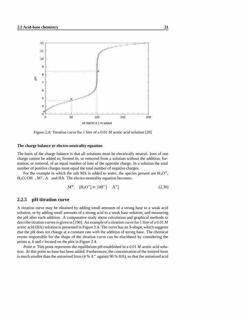
A titration curve may be obtained by adding small amounts of a strong base to a weak acidsolution, or by adding small amounts of a strong acid to a weak base solution, and measuringthe pH after each addition. A comparative study about calculation and graphical methods todescribe titration curves is given in [190]. An example of a titration curve for 1 litre of a 0.01Macetic acid (HA) solution is presented in Figure 2.4. The curve has an S-shape, which suggeststhat the pH does not change at a constant rate with the addition of strong base. The chemicalevents responsible for the shape of the titration curve can be elucidated by considering thepointsa, b andc located on the plot in Figure 2.4.
Point a: This point represents the equilibrium pH established in a 0.01M acetic acid solu-tion. At this point no base has been added. Furthermore, the concentration of the ionized formis much smaller than the unionized form (4 % A� against 96 % HA), so that the unionized acid
22 Chemical aspects of pH buffer capacity
concentration can be considered almost equal to the initial concentration. Calculation detailsof this example are given in section 3.2.1 on page 40 (e.g. initial pH, which is 3.36 in this case)
Point b: This point represents the pH established when the concentration of unionized acidequals the concentration of the ionized acid; i.e.,
[HA] = [A�] (2.37)
The validity of equation (2.37) can be substantiated by considering the Henderson-Hasselbachequation (equation (2.21)) for the acetate buffer. When the measured solution pH is equal tothe acidpKa value, equation (2.21) reduces to
log[A�]
[HA]= 0 (2.38)
which holds when[A�] = [HA]. An examination of the titration curve in the vicinity of pointb also shows that, around this point, the solution pH will show the smallest change per unit ofstrong base added. In other words, the pH buffering effect is the highest at pointb. Because ofthis effect, the useful range of a buffer system is practically around 1.5 pH units on either sideof its pKa value.
Point c: This point represents the pH established when the concentration of ionized acidapproaches the initial acid concentration, thus[A�]�= 0:01M. 3 In other words, the pH at thispoint is the equivalence-point for a 0.01M acetate salt solution. Further addition of a strongbase past pointc will result in a continued increase in pH. The limiting pH is set by the pH ofthe titrant. In Figure 2.4 it is assumed that a 0.1M NaOH (which is at pH 13) is used as thetitrant. Thus, when the effects of dilution become insignificant, the pH will approach 13.
In the previous example, only 1 monoprotic4 buffer system in an aqueous solution wasconsidered. A titration curve can also be obtained by adding small amounts of strong base toa solution, containing more than 1 buffer system, including polyprotic buffers. An example ofsuch more complex titration curve is shown in Figure 2.5. The difference with the previousexample is that the pointsa, b andc cannot be distinguished for the individual buffers on thegraph. The mathematical aspects of this type of titration curves will be handled in chapter 3.A graphical method to determine thepKa for simple titration curves is given in [189].
2.2.6 pH buffer capacity curve
The slope of a titration curve (pH versusCB or CA) is related to the tendency of the solutionat any point in the titration curve to change the pH upon addition of base or acid. The bufferintensity at any point of the titration is inversely proportional to the slope of the titration curveat that point and may be defined as [273]:
β =dCB
dpH=� dCA
dpH(2.39)
3Theoretically, even at high pH values, there is always a small fraction of the unionized acid[HA].4A monoproticconjugate acid-base pair, HA�A�, can interchange 1 proton.

2.2 Acid-base chemistry 23
3
4
5
6
7
8
9
10
11
0 10 20 30 40 50
pH
ml NaOH 0.1 N added
Figure 2.5: Titration curve for 1 litre of a more complex aqueous system containing 5mgCO2 l�1, 7 mg o-PO4-Pl�1, 15mgNH+
4 -N l�1 and 0.6meq l�1 of an unspecified soap
β : buffer intensity (eq l�1 pH�1)dCB, dCA : differential quantity of strong base or acid added (eq l�1)dpH : differential change in pH due to addition ofdC
Note thatβ is always positive.A graphical representation ofβ as a function of pH may be obtained by plotting the inverse
of the slope of the titration curve versus pH. The buffer capacity curve corresponding withthe titration curve in Figure 2.4 is shown in Figure 2.6. The point with the highest buffercapacity, excluding the water buffer is pointb, the top of the buffer capacity profile. For buffersystems withpKa values lower than 4 or higher than 10, the maximum of the bell-shaped bufferintensity profile does not necessarily correspond with thepKa value of that buffer system,due to the presence of the buffer capacity of the water solution (see an example in the nextparagraph).
The buffer capacity curve, corresponding with the titration curve in Figure 2.5 is shown inFigure 2.7. The different buffer systems that contribute to the buffer capacity curve are sepa-rately indicated on the graph. This also illustrates the additive behaviour of buffer capacities:The overall buffer capacity of the solution is the sum of buffer capacities of the different con-stituents to this solution. It can be noted on the graph that the maximum of the overall buffercapacity profile around pH 9 does not exactly correspond with thepKa of ammonium, althoughit is the most important buffer at that pH position. A mathematical model ofβ will enable tosimulate buffer capacities, and thus predict the buffer behaviour of solutions. This is the topicof chapter 3.

24 Chemical aspects of pH buffer capacity
0
2
4
6
8
10
3 4 5 6 7 8 9 10 11 12
Buf
fer
capa
city
(m
eq l-1
pH
-1)
pH
a
b
c
Figure 2.6: Buffer capacity curve for a 0.1M acetic acid solution
0
0.1
0.2
0.3
0.4
0.5
0.6
0.7
4 5 6 7 8 9 10
Buf
fer
capa
city
(m
eq l-1
pH
-1)
pH
total buffer capacity55.5 M water5 mg CO2 l-1
7 mg o-PO4-P l-1
15 mg NH4-N l-1
0.0006 M soap
Figure 2.7: Buffer capacity curve for a more complex aqueous system containing 5mgCO2 l�1,7 mg o-PO4-Pl�1, 15mgNH+
4 -N l�1 and 0.6meq l�1 of an unspecified soap

2.3 Dissolved organic carbon 25
2.3 Dissolved organic carbon
The most important acid-base system in water is often the carbonate buffer. The chemicalspecies that make up the carbonate system are gaseous CO2 (CO2(g)), aqueous or dissolvedCO2 (CO2(aq)), carbonic acid (H2CO3), bicarbonate (HCO�3 ), carbonate (CO2�3 ) and carbon-ate containing solids. Consequently, the carbonate system is the most important buffer innatural waters. In addition, individual species are of interest to us because they participate inimportant reactions other than strictly acid-base interactions [263]. Carbon dioxide is a partic-ipant in the biological processes of respiration (CO2 produced) and biosynthesis by autotrophssuch as nitrifiers or photosynthetic organisms (CO2 consumed). The dissolution of CO2 fromthe atmosphere into water or the release of CO2 from supersaturated waters involves a hetero-geneous reaction between gas and liquid phases. Similarly, the carbonate ion participates inheterogeneous reactions with solids containing carbonate, notably calcium carbonate.
2.3.1 The carbonate species and their acid-base equilibria
When we are presented with a problem involving the carbonate system, we must first make adecision concerning the nature of the system. This step is important because carbonate speciescan be involved in homogeneous solution equilibria as well as heterogeneous gas/liquid andliquid/solid equilibria [263]. The system can be treated as (ordered by increasing complexity):
� a closed system with no solid present,� an open system with no solid present,� a closed system with solid present, and� an open system with solid present.
For the moment we will neglect the equilibria between carbonate species and metal ions(see section 2.4) and the involvement of carbonate-containing solids (see section 2.5), and treatthe carbonate system as an open system with no solid present. Assuming a temperature of 25oC, the following equilibria can be considered [263]:
CO2(g)+H2OCO2(aq) K = KH = 10�1:5 M atm�1 (2.40)
CO2(aq)+H2OH2CO3 Km = 10�2:8 (2.41)
H2CO3 H++HCO�3 K†
1 = 10�3:5 (2.42)
H2CO�3 H++HCO�
3 Ka1 = 10�6:3 (2.43)
HCO�3 H++CO2�
3 Ka2 = 10�10:3 (2.44)
KH stands for Henry’s constant. From equation (2.41) it is concluded that the concentrationof hydrated carbon dioxide, CO2(aq), predominates over the concentration of carbonic acid,H2CO3:
Km = 10�2:8 =[H2CO3]
[CO2(aq)]= 1:6�10�3 (2.45)

26 Chemical aspects of pH buffer capacity
Table 2.3: Reaction rates within the carbonate system [198,273]
Reaction Forward ratevf Backward ratevr
CO2(g)+H2O CO2(aq) 6�10�9mol cm�2 s�1 a
CO2(aq)+H2OH2CO3 0.025�0.04s�1 (20�25 oC) 10�20s�1 (20�25 oC) b
CO2(aq)+OH�HCO�
3c 8:5�103M�1 s�1 2�10�4s�1 d
H2CO3 HCO�3 +H+ 1:5�107s�1 e 4:7�1010M�1 s�1
a Calculated for the situation of a typical lake.b The ratio ofvf andvr corresponds withKm (see equation (2.41)).c This reaction is kinetically insignificant at pH< 8.d The ratio ofvf andvr corresponds withKa1Kw (see equation (2.43)).e Calculated fromvr andK†
1 (see equation (2.42)).
Thus [H2CO3] is only 0.16 % of[CO2(aq)]. Because it is difficult to distinguish betweenCO2(aq) and H2CO3 by analytical procedures such as acid-base titration, a hypothetical speciesH2CO�
3 is used to represent H2CO3 plus CO2(aq). The composite equilibrium constantKa1 of
equation (2.43) is a result of the product ofKm (equation (2.41)) andK†1 (equation (2.42)). The
implications of this development are important because they point out that H2CO3 is a fairlystrong acid (K†
1 = 10�3:5), but there is very little of it in solution. This point is emphasizedbecauseKa1 is 10�6:3, a value that would give the impression that carbonic acid is a very weakacid. Carbonic acid has some of the properties of a strong acid, like the dissolution of mineralsby CO2. Throughout this text we will use the hypothetical species H2CO�
3 to represent CO2(aq)plus H2CO3. We will treat it as a diprotic acid, but we should keep in mind its true nature.
As discussed earlier (section 2.2.1), acid-base equilibria are from a kinetical point of viewextremely rapid, except for the carbonate system equilibria, and this in open as well in closedsystems. The explanation of this behaviour lies in the slow (relatively to other deprotonationreactions) rate of hydration of aqueous CO2. The hydratation of CO2(aq) leads to H2CO3
(equation (2.41)), but it may also yield H+ and HCO�3 [273]. The individual rate constantscannot be experimentally resolved and are reported simply askCO2 andkH2CO3 correspondingto the simplified scheme:
CO2(aq)+H2OkCO2
kH2CO3
H2CO3very fast H++HCO�
3 (2.46)
An overview of reported rate constants for the carbonate system is given in Table 2.3. It hasto be noted that the values in Table 2.3 are given as approximative values because they aredependent on many different factors. For the equilibrium where H2CO�
3 is involved (equation(2.43)), no rate constants are given, because this equation is a ‘pooled’ equation, where a veryfast proton exchange reaction, as well as a relatively slow hydratation/dehydratation reactionare involved. More details about these reaction rates can be found in [198, 273].

2.3 Dissolved organic carbon 27
Figure 2.8: Aqueous carbonate equilibrium; atmosphericpCO2 and 25oC; pH adjusted withstrong base or acid;CT represents the sum of the solute carbonate species; point P showsequilibrium concentrations without pH adjustments [273]
A simple system illustrating some of the characteristics of the carbonate system in naturalwaters is provided by equilibrating pure water with a gas phase (e.g. the atmosphere) contain-ing CO2 at a constant partial pressure. One may then vary the pH by the addition of strong baseor strong acid, thereby keeping the solution in equilibrium withpCO2. Figure 2.8 shows the dis-tribution of the solute species in such a system. A partial pressure of CO2 (pCO2 = 10�3:5atm)is representative for the atmosphere. When this is in equilibrium with CO2(aq), we obtain fromequations (2.40) and (2.45):
[H2CO�3]�= [CO2(aq)] = KH � pCO2 = 10�1:5�10�3:5 = 10�5 M (2.47)
2.3.2 Alkalinity and acidity
Alkalinity is a measure of the capacity of a water to neutralize strong acid. In natural watersthis capacity is attributable to bases such as HCO�
3 , CO2�3 and OH� as well as to species often

28 Chemical aspects of pH buffer capacity
present in small concentrations such as silicates, borates, ammonia, phosphates, and organicbases [263].Acidity is a measure of the capacity of a water to neutralize strong base. In naturalwaters this capacity is usually attributable to acids such as H2CO�
3 and HCO�3 and sometimesto strong acids, namely, H+ [263].
Operational definition of alkalinity
In the determination of the total alkalinity a known volume of sample is titrated with a standardsolution of a strong acid to a pH value in the approximate range of 4 to 5 and usually in therange 4.5 to 4.8. This end-point is commonly indicated by the colour change of the indicatormethyl orange; therefore the total alkalinity is often referred to as the methyl orange alkalinity.Alkalinity can be expressed asmeq l�1 or asmgCaCO3 l�1. In the latter case, one takes intoaccount that 1meqof CO2�
3 requires 2meqof H+, so that 1meql�1 = 50mgCaCO3 l�1. If weconsider first a closed system in which the alkalinity contributing species are only carbonateand OH�, then the H+ added is the stoichiometric amount required for the following reactions:
H++OH� H2O (2.48)
H++HCO�3 H2CO�
3 (2.49)
2H++CO2�3 H2CO�
3 (2.50)
The pH at the true end-point of the total alkalinity titration should be that of a solution ofH2CO�
3 and H2O. We refer to the pH of such a solution as pHCO2.For the carbonate system, we can theoretically identify two more significant pH values
that occur during the course of an alkalinity titration. These are pHHCO�
3and pHCO2�
3. They
represent, respectively, (1) the pH of a solution to which has been added the stoichiometricamount of H+ required to complete5 reaction (2.48) and the following reaction:
H++CO2�3 HCO�
3 (2.51)
and (2) the pH of a solution to which has been added the stoichiometric amount of H+ requiredto complete only reaction (2.48). The value of pHHCO�
3is about pH 8.3 while pHCO2�
3is gen-
erally between pH 10 and pH 11 and varies with the amount of carbonate buffer present. Theexperimental amount of acid required per litre of solution to lower the pH of this solution topHHCO�
3is called the carbonate alkalinity. This end-point can be determined with a pH meter
or by a colour change of the indicator phenolphthalein so that it is often referred to as the phe-nolphthalein alkalinity. The amount of acid required to reach pHCO2�
3(the caustic alkalinity)
cannot be determined readily in the laboratory because of the poorly defined end-point, causedby the masking effect of the buffering of water (i.e. the reaction H++OH�
H2O). Caustic
5Theoretically, equilibrium reactions are never completed, however, operationally a reaction is completed when anequivalence-point is reached. See also section 2.2.5.

2.4 Metal ions in aqueous solution 29
Table 2.4: End-point pH values for total alkalinity measurements [104]
Test condition End-point pH
Alkalinity 30 mgCaCO3 l�1 4.9Alkalinity 150 mgCaCO3 l�1 4.6Alkalinity 500 mgCaCO3 l�1 4.3Silicates, phosphates known/suspected 4.5Routine or automated analysis 4.5Industrial waste or complex system 4.5
alkalinity can be determined by calculation if the carbonate and the total alkalinity are known[263].
The actual values that correspond to pHCO2, pHHCO�
3and pHCO2�
3are not truly fixed values,
rather they vary with the total inorganic carbon buffer concentrationCIC in solution. If we treatthe titrations as closed systems, theCIC at the end-point will be the same as theCIC in the initialsolution. This appears to be a reasonable approach if the solution is not shaken vigorously andif the titration is conducted rapidly. Table 2.4 shows theStandard Methods[104] values for thetotal alkalinity end-points in function of the sample and itsCIC concentration.
Similar definitions and calculations concerning acidity measurements can be made. How-ever, in the scope of this work, we will mainly work with the alkalinity and not with the acidity.
2.4 Metal ions in aqueous solution
Complex formation is important in the chemistry of natural waters and wastewaters from sev-eral standpoints. Complexes modify metal species in solution, generally reducing the freemetal ion concentration so that effects and properties which depend on free metal ion con-centration are altered. These effects include such things as the modification of solubility, thetoxicity and possibly the biostimulatory properties of metals [155, 263]. Complexation equi-libria will also influence the buffer capacity, which is the reason of discussing this topic here.
In aqueous solution,free metal ions are complexed with water. The metal ions are saidto be hydrated. The interaction of these hydrated metal ions with acids and bases is a ligandexchange reaction that is commonly called hydrolysis or protolysis. These terms describe thegeneral reaction in which a proton is transferred from an acid to water, or from water to abase. This type of reaction involving hydrated metal cations occurs readily and is of extremeimportance in natural waters [263]. For example, the first step of the stepwise hydrolysis ofthe hydrated ferric ion, Fe(H2O)3+
6 can be represented by the following equation:
Fe(H2O)3+6 +OH�
Fe(H2O)5OH2++H2O (2.52)
From this equation it is easy to visualize that the hydrolysis of metal ions is a stepwise replace-ment of coordinated molecules of H2O by hydroxyl ions. The hydrolysis reaction depicted in

30 Chemical aspects of pH buffer capacity
equation (2.52) is an acid-base (proton transfer) reaction. Because of this, the pH of the solu-tion will influence the distribution of the various species, and the presence of such reactionswill influence the buffer capacity of the water. All trivalent and most divalent metal ions arecomplexed to some extent with OH� at the pH of natural waters. The alkaline earth metalshydrolyse significantly only at high pH (pH> 9).
2.4.1 Complex formation and dissociation constants
Equilibrium constants for complexes can be written in many different ways. In literature it isnot always consistent and clear what kind of constant is used and how it has to be interpreted.A minimal care has to be taken when using and interpreting values from literature. Somepopular different ways of expressing complex equilibria and some examples to illustrate theconfusions are presented here.
Equilibrium constants for complexes are usually stated for reactions written in the directionof complex formation, e.g.,
Ca2++PO3�4 CaPO�4 (2.53)
and
fCaPO�4 gfCa2+gfPO3�
4 g = 10+6:5 = stability constant (2.54)
When stated for a complex formation reaction, the equilibrium constant is called aformationor a stability constant. Conversely, if the equilibrium constant is stated for the dissociationof the complex it is called adissociationor aninstability constant. Large values of stabilityconstants indicate stable complexes.
For complexes that contain more than one ligand or central metal ion, there are two waysof writing stability constants. Stepwise formation constants are equilibrium constants for thereactions in which the central metal ion consecutively adds one ligand (symbolK). An overallformation constant is the equilibrium constant for the reaction in which the central metal ioncombines with all of the ligands necessary to form a specific complex (symbolβ) [263]. It isalso common to omit the H2O ligands when writing equations such as this one given here. Forexample Fe(H2O)5OH2+ is usually written as FeOH2+.
Furthermore, the equation (2.52) shows hydrolysis reactions as a replacement of a water ofhydration by a hydroxyl ion. Such reactions can also be written as a transfer of protons fromwaters of hydration to free water molecules to form a hydronium ion. The symbols for thestability and overall stability constants are often represented as�K and�β respectively [273].For example, the reaction (2.52) can be written as
Fe(H2O)3+6 +H2O Fe(H2O)5OH2++H3O+ (2.55)
or as
Fe(H2O)3+6 Fe(H2O)5OH2++H+ (2.56)
2.4 Metal ions in aqueous solution 31
with formation constants for equations (2.52) and (2.56) respectively:
K1 =fFe(H2O)5OH2+gfFe(H2O)3+
6 gfOH�g = 10+11:84 (2.57)
�K1 =fFe(H2O)5OH2+gfH+g
fFe(H2O)3+6 g = 10�2:16 (2.58)
Generally one can write that�K1 = K1�Kw. A consistent overview of the nomenclature usedfor complexation constants can be found in [216].
To illustrate the confusions found in aquatic chemistry literature when looking up stabilityconstants for complex formation, an example of complex formation between Ca2+ and H2PO�
4is presented. One of the popular tables found in modern aquatic chemistry textbooks is the oneoriginally presented by Morel and Hering [198] and taken over in other reference works like[273] and [251]. A major issue presented by the original authors is data consistency [198]:For example, a complex formation constant reported by one author may have been calculatedon the basis of a solubility constant that is not the same as that chosen in the compilation.Crosschecking the methods for estimating the constants from experimental data is advised.This can explain already some of the inconsistencies in literature, but there are also otherfactors that lead to wrong interpretation. For the example given here, one can find in [273]and [251] for the metal Ca2+ and the ligand PO3�4 (notated with L) (note that H2PO�
4 is notpresented as possible ligand) that the logarithm of the overall stability constant for formationof the complex CaH2L equals 21.0. With the information presented above, one may wish towrite the following equation:
Ca2++H2PO�4 CaH2PO+
4 (2.59)
with the corresponding stability constant
K1 = β1 =fCaH2PO+
4 gfCa2+gfH2PO�
4 g= 10+21:0 (2.60)
However, this is not correct, because only when consulting the table of the original authors[198], one finds that the only correct way of writing this complexation reaction is
Ca2++2H++PO3�4 CaH2PO+
4 (2.61)
with the correct corresponding stability constant
K1 = β1 =fCaH2PO+
4 gfCa2+gfH+g2fPO3�
4 g = 10+21:0 (2.62)
In an older reference [48] a reaction was found which corresponds with our example:
Ca2++H2PO�4 CaH2PO+
4 logK = 1:08 (2.63)

32 Chemical aspects of pH buffer capacity
which logically corresponds to the following equation forK1
K1 = β1 =fCaH2PO+
4 gfCa2+gfH2PO�
4 g= 10+1:08 (2.64)
When reaction (2.63) is summed with the 2 following reactions for the acid-base equilibria ofthe ortho-phosphate buffer system:
H++HPO2�4 H2PO�
4 logK = 7:2 (2.65)
H++PO3�4 HPO2�
4 logK = 12:35 (2.66)
one finds the same reaction as (2.61) and a logK value equal to 1:08+7:2+12:35= 20:62�21, thus corresponding toK1 in equation (2.62).
For the same example, another aquatic chemistry book [263] gives the following reaction(written as a dissociation instead of a formation reaction):
CaH2PO+4 Ca2++H++HPO2�
4 pK =�5:6 (2.67)
The reaction can easily be transformed into a complex formation reaction:
Ca2++H++HPO2�4 CaH2PO+
4 logK =�5:6 (2.68)
From this equation we can write
K1 = β1 =fCaH2PO+
4 gfCa2+gfH+gfHPO2�
4 g = 10�5:6 (2.69)
Summing reaction (2.68) with reaction (2.66) one finds
K1 = β1 =fCaH2PO+
4 gfCa2+gfH+g2fPO3�
4 g = 10�5:6+12:35= 10+6:75 (2.70)
The logK of equation (2.70) is not the same as the logK of equation (2.62), there is a differenceof approximately 14 log units in the two logK values, indicating that one of the 2 equationsis not correctly presented into the literature. Assuming the reference work [198] and also [48]are correct, one might eventually suggest that in [263] the author presented�K values insteadof K values, but without mentioning it into the presented equation.
This illustrative example learns that there are many different ways of writing complexationreactions, and that different notations andK values eventually represent the same complexationreaction when using extra water or ligand dissociation reactions, and that extreme caution isneeded when using values from tables in which it is not straightforward to assess what thetabulated values exactly mean.

2.4 Metal ions in aqueous solution 33
Table 2.5: Percentage distribution of complex species in average river water [263]
Complexed with (%)
Cation Concentration (M) Uncomplexed (%) OH� HCO�3 CO2�
3 SO2�4
Calcium 3:8�10�4 97 1 1 1Magnesium 3:4�10�4 97 1 1 1Sodium 2:7�10�4 100Potassium 5:9�10�5 100
2.4.2 Complexes with inorganic ligands
Natural waters contain significant concentrations of inorganic and organic ligands in additionto H2O and OH�. The predominant metal cations in typical fresh water are Na+, Ca2+ andMg2+; the major ligands are HCO�3 , Cl� and SO2�
4 . At the typical natural water pH valuesbetween 6.5 and 8.5, these metals are no strong complex formers as Al3+ and Fe3+ [263].
For complicated systems such as natural waters it is necessary to use a computer pro-gram/model to determine the degree of complexation of the various cations with the ligandsavailable. The results of a simulation study on a river water with average composition is shownin Table 2.5 [263]. This type of calculation gives us confidence in ignoring the complexes ofCa2+, Mg2+, Na+ and K+ with OH�, HCO�
3 , CO2�3 , SO2�
4 and Cl�, when dealing with freshwaters of neutral pH. Increasing the pH-value or ligand concentration (like in a titration exper-iment), may require though that complexes of these metals be taken into consideration.
2.4.3 Complexes with organic ligands
A wide variety of organic compounds in natural waters and wastewaters can act as complex-ing agents for metal ions. The nature and extent of metal ion complexation by natural waterorganics is not well defined, probably because of the poorly defined nature of these organiccompounds and also because of the staggering complexity of these multimetal, multiligandsystems [263]. Two categories of significant organic complexes in river waters are the ‘aminoacid complex’ and ‘inert humic complex’. For the most amino acid complexes, the values oflogβ1 range from 7 to 9; values of logβ2 are in the approximate range of 14 to 16. Howeverthere are again some exceptions, e.g. the amino acid cysteine, which contains an�SH group,forms an extremely strong complex with cuprous ion (Cu+) with a logβ1 value of 19.5. Humicsubstances are an extremely complex group of compounds. Because of this no single com-pound can act as a true model for this group. However, phenolic (pKa 8.5�11) and carboxylicacid (pKa 3�6) groups are common functional groups in humic substances [226].
Humic substances or humates are a mixture of poorly biodegradable decomposition prod-ucts and by-products of natural organic matter produced by plants and animals. They arenatural constituents of surface water, especially in regions with a cold climate, since low tem-perature is a condition for the formation of water-extractable humic substances [185]. Humicsubstances have been arbitrarily divided into three diverse groups of compounds on the basis

34 Chemical aspects of pH buffer capacity
of their solubility in dilute acid and dilute base.Fulvic acidsare soluble in both dilute acid(pH 1) and dilute base.Humic acidsare soluble in dilute base but are precipitated by diluteacid (pH 1).Humin is insoluble in both dilute acid and dilute base. It is the fulvic acid frac-tion that appears to be the predominant group of humic substances in natural waters. Fulvicacids appear to have lower molecular weights (200 to 10000) than humic acids; they contain ahigher percentage of oxygen and the oxygen appears to be located in a greater percentage ofcarboxyl groups. Fulvic acids, in particular, are good complexing agents for trace metals innatural waters [251]. Fulvic acid binding of trace metals is complicated. Not only is fulvic acida distribution of a wide range of molecules, it has a variety of binding sites that are affected bypH, ionic strength, and the chemistry of ions in solution.
When chemical equilibrium models are used to assess e.g. toxicity induced by free metalions, fulvic acid complexation should be taken into account [81], especially for metals withlarge logK values for metal-fulvate complexes such as Hg2+, Cu2+, Pb2+ and Cd2+. Com-plexation of metals with fulvic acid is most significant for those ions that are appreciablycomplexed with CO2�3 and OH� [251]. When chemical equilibria are used for buffer capacitymodelling, it are the metal ions with the highest concentrations that have to be considered first.Acid-base titrations of humic substances reflect the nature of the differentpKa values, hencethe ‘smeared out’ appearance of these titration curves. While no unique equivalence-points areobserved, differentpKa regions of carboxylic and phenolic groups can be discerned [273]. Ina study based on titration curves of dissolved organic carbon (DOC) in wastewater, two acid-ity constants, 5.3 and 9.5 were found to be attributed to DOC [331]. FTIR spectra suggestedthe acid sites are carboxylic and amino functional groups. In the River Vouga (Portugal), thepresence of sulphonic functional groups in the fulvic acids were found to origin from a pulpand paper mill effluent, that was discharged in that river [247]. These results highlight theimportance of the contribution of anthropogenic sources of organic matter to the compositionof humic substances from surface waters.
For describing chemical equilibria between metal ions and e.g. fulvic acid, a conditionalstability constant approach can be used [251]:
M+FAM�FA Kc =[M�FA][M][FA]
(2.71)
whereKc is the conditional stability constant at a specified pH, ionic strength, and chemicalcomposition. One does not always know the stoichiometry of the reaction in natural waters, e.g.whether 1:1 complexes (M�FA) or 1:2 complexes (FA�M�FA) are formed. The complexantis a macromolecule of organic carbon in which there are many different sites with varyingbinding energies. So, equation (2.71) simply gives a lumped-parameter conditional stabilityconstant, but it does allow intercomparisons of the relative importance of complexation amongdifferent metal ions and dissolved organic carbon (DOC) at specified conditions. Conditionalstability constants for metal-fulvic acid complexes vary in natural waters because:
� There are a range of affinities for metal ions and protons in natural organic matter result-ing in a range of stability constants.
� Conformational changes and changes in binding strength of M�FA complexes in naturalorganic matter result from electrostatic charges (ionic strength), differential and compet-itive cation binding, and, most of all, pH variations in water.

2.5 Precipitation and dissolution reactions 35
The total number of metal-titratable groups is in the range of 0.1�5 meqper gram ofcarbon, and is termed the DOC complexation capacity. DOC comprises roughly 90 % of thetotal organic carbon in surface waters, most of which is recalcitrant [294].
Rather than using a conditional complexation constant or a distribution of discrete com-plexation constants, an alternative approach is to use ax-site model, withx different ligands(sites), andx different stability constants. This approach with e.g.x = 5 can be used to de-scribe the complexation of dissolved fulvic acid and copper ions in natural water [251]. Manyinvestigators have used a two site model representing fulvic acid functional groups with acidityconstantspKa1 � 3:5 andpKa2 � 5:0 [251].
In a third approach for describing chemical equilibria between metal ions and humates, thehumates can be described by a mixture of ligands with a continuous (Gaussian) distributionof acidity or metal-binding constants [198]. Two centres ofpKa distributions in this Gaussianapproach (around pH 3 and pH 5) were found to describe the buffering capacities of humicacids fairly well [82]. In a study of the organic contribution to alkalinity in estuarine waters,it was found that humic substances have a buffer capacity around pH 4.5, pH 6.6 and pH 8.9[49]. The authors suggest that the first two groups are carboxylic acids, and group three maybe phenols or amines.
2.5 Precipitation and dissolution reactions
Precipitation and dissolution reactions are important in both natural waters [263] and watertreatment processes, more particular in e.g. phosphorus removal [72, 83, 200, 346]. Dissolu-tion of minerals is a prime factor in determining the chemical composition of natural waters.Both equilibrium considerations and the rates of reactions are important. In many instancesthe reaction rate controls the extent of reaction because insufficient time is available for equi-librium to be achieved. This will have important drawbacks when precipitation reactions willbe considered in titration experiments. A number of caveats are in order before embarking onthe study of solubility relationships in aquatic systems [198]:
1. Many precipitation-dissolution reactions are sluggish. For example, a large supersatu-ration of CaCO3 is often observed in natural waters before precipitation of the solidsactually occurs. Temperature, the presence of nucleating surfaces and biological activitycan all dramatically alter precipitation-dissolution kinetics.
2. The solid formed is often not the most stable solid thermodynamically. The evolution ofthe solid to its more stable form (e.g. through recrystallization) is usually very slow.
3. The metastable solids that are initially precipitated are often ‘non-stoichiometric’. Manynatural solids also typically contain impurities, foreign ions incorporated in the matrix.The equilibrium constants used for such solids have operational value, but probablylittle true thermodynamic significance. There is a wide variation in the reported valuesof heterogeneous equilibrium constants.
4. The formation of pure solid phases is not the only, or perhaps even the dominant, processby which many solutes are removed from the solution. For example, surface adsorptioncan remove a solute from solution much below saturation conditions for pure solids.

36 Chemical aspects of pH buffer capacity
Precipitation has generally been observed to occur in three steps:
� nucleation (homogeneous if nuclei are formed with the ions of the precipitate; or hetero-geneous if foreign particles act as nuclei),
� crystal growth, and� agglomeration and ripening of the solids.
The formation of nuclei from precipitate ions is an energy-consuming process, so solutionshave to be supersaturated, or have concentrations greater than that predicted by equilibriumwith the precipitate, before the precipitate will form from a homogeneous solution.
At the outset of any discussion on heterogeneous equilibria it is important to realize thatheterogeneous calculations only apply when there is is anexcess of the solidof interest present.If solid is absent, the equilibrium calculations are not valid for predicting solution composition;they may only be used to test whether saturation with a particular solid exists. Although ther-modynamic considerations will yield the driving force for precipitation of particular phases,their formation under a specific set of conditions may be determined much more by kineticfactors. Metastable phases may persist in supersaturated solutions [204].
The solubility product
The solubility product is the equilibrium constant that describes the reaction by which a pre-cipitate in excess dissolves in pure water to form its constituent ions [263],
AzBy(s) zAy++yBz� (2.72)
The solubility constant is defined as
Ks0 =fAy+gzfBz�gy
fAzBy(s)g(2.73)
The activity of the solid phase is taken as unity. The concentration product, or conventionalsolubility product [273], logcKs0, has the same form as the equilibrium constant except thatconcentrations of the species in solution are used instead of their activities.
log cKs0 = [Ay+]z[Bz�]y (2.74)
For the solubility of oxides and hydroxides, the symbol logc�Ks0 [273] can be used insteadof log cKs0, when the solubility equilibrium is expressed in terms of[H+] instead of[OH�].Similar as in section 2.4.1, caution is needed when values from the literature are used.
Available compilations of solubility products illustrate that values given by different au-thors for the same solubility products often differ markedly. Differences of a few orders ofmagnitude are not uncommon [273]. There are various reasons for these discrepancies, forexample the higher complexity of solubility equilibria compared to e.g. acid-base equilibria;and the presence of solubility influencing species not accounted for in theKs0.
In order to test whether a solution, or a natural water, is over- or undersaturated, the actualion activity product (IAP), may be compared withKs0 [273]. E.g. for the solidAzBy(s), the IAPequalsfAy+gzfBz�gy The state of saturation of a solution with respect to a solid is defined as:

2.6 Modelling tools 37
� IAP > Ks0: oversaturated� IAP = Ks0: equilibrium, saturated� IAP < Ks0: undersaturated
2.6 Modelling tools
For finding solutions of a ‘large’, natural water system equilibrium model, having many reac-tions and many species, hand calculations are extremely slow and essentially infeasible [273].Computers have enabled rapid computations of equilibrium composition for multicomponent,multiphase, multispecies systems [273].
Two approaches to the treatment of large systems have been developed: the Gibbs energyminimization method and the equilibrium constant approach [13, 262, 273]. Both are based ona knowledge of the chemical potentials of species under standard conditions and under actualconditions of compositions in the chemical system. In the Gibbs energy minimization ap-proach, one guesses a solution to the equilibrium problem (the free concentrations of species)and proceeds to minimizeGTOT. In the equilibrium constant approach, one guesses the freecomponent concentrations, solves the non-linear equilibrium equations for the species concen-trations, and verifies the total component material expressions or mass balances. If differentprecipitation reactions have to be considered in one model, a thermodynamic based solutionapproach is preferred, rather than an equilibrium based solution approach [177]. However, ifsome free energies for particular components are missing, the free energy methods cannot beused [13].
Chemical modelling in hydrologic systems has become an area of active research with im-mediate opportunities for application to environmental problems [24]. There are many com-puter models available for chemical equilibrium calculations. A number of these packages arereviewed in [24]. New concepts in modelling which provide innovative advancements includemodel sensitivities, sampling and analytical error, computational errors, redox and metastabil-ity, thermodynamic and kinetic data advance,: : : One of the more recent models, that hasfound wide use among environmental professionals is MINTEQA2 [10, 251]. It is freelyavailable (public domain software) and well documented. MINTEQA2 has been supportedby the U.S. Environmental Protection Agency Environmental Research Laboratory, Athens,Georgia. This package is suitable for chemical equilibrium problems in natural water (acid-base, precipitation-dissolution, complexation, surface complexation and redox reactions). It’sdatabase contains thermodynamic data for 1000 species, and can be supplemented with a userdefined thermodynamic database. Partly due to the reasons mentioned in section 2.5, precipi-tation reactions are sometimes very difficult to model with chemical speciation programs likeMINTEQA2 [176,198]. For instance, in lead precipitation tests from aqueous solutions con-taining sulphate, quasi equilibrium conditions between soluble and solid phases were achieveda few hours or days after reagents blending. Significant discrepancies were found between fil-terable lead concentrations measured in aged precipitate suspensions and solubility predictionsby MINTEQA2 [176]. Further, a flexible thermodynamic database is important to allow theuser to modify e.g.K-values, because these values are case dependent [187]. Also, it is knownthat the precision of thermodynamic data values varies from excellent to poor, so such data issubject to constant revision [85].
38 Chemical aspects of pH buffer capacity
Despite the wide experience with the MINTEQA2 thermodynamic database, this databasestill contains errors that can lead to significantly erroneous results. An example of a recentlycorrected significant error in reactions with organic ligands is illustrated with Cu�EDTA spe-ciation [257]. Two typical types of errors were discovered in the thermodynamic database ofMINTEQA2 [257]:
� Errors related to expressing the reaction in terms of MINTEQA2 components: All reac-tions in MINTEQA2 must be written as formation reactions. For solid species, the logKand∆H0, needed in MINTEQA2, may be of the opposite sign to that reported in the lit-erature (usually reported as a solubility product constant). Also both solid and dissolvedreactions obtained from the literature and their associated thermodynamic constants mayneed to be added or subtracted from other reactions as required to reformulate the reac-tion in terms of MINTEQA2 components. Similar findings of confusion in the literatureare also illustrated in section 2.4.1.
� Errors related to ionic strength and temperature correction of logK. All log equilibriumconstants in the database must be referenced to zero ionic strength and to 25oC.
A reactive solute transport model in streams, coupled to a chemical equilibrium modelbased on MINTEQA2 was used for river water modelling [243, 244]. The equilibrium sub-model considers the speciation and complexation of aqueous species, precipitation, dissolutionand sorption. The model provides a valuable tool for quantifying the nature and extent of pH-dependent processes within the context of hydrologic transport [244]. Alkaline precipitationand aging of Cu2+ in the presence of sulphate was investigated with MINTEQA2, in the frame-work of recovery of copper from industrial wastewaters and sludges [177]. A MINTEQA2model with 2 ammonia species, and respectively 21 copper or 18 nickel species was used toassess the effect of these heavy metals on nitrifying bacteria [149]. Surface complexation andprecipitation modelling using MINTEQA2 was successfully applied to describe the leachingof contaminants from weathered municipal solid waste incinerator bottom ash [187].

Chapter 3
Mathematical pH buffer capacitymodelling
3.1 Introduction
In literature, various approaches are considered to model pH buffer capacity [198, 251, 263,273]. Depending on the aim of the modelling, a different approach can be necessary. However,the majority of approaches focus on assessing the composition or species distribution (includ-ing pH) of a sample under a certain set of conditions. A simple example illustrates the types ofquestions asked: A solution contains 5mmolof acetic acid, we add 5ml of NaOH 0.1N to thissolution, what will be the pH at equilibrium? This we could call a single point analysis, thesituation of 1 equilibrium point only is considered. This problem can be extended, consideringconsecutive small additions of NaOH to our acetic acid sample, resulting in a titration profile,where pH is a function of the amount of base added. Some chemical aspects of pH titrationare presented in chapter 2, more particularly in section 2.2.5 on page 21 and section 2.2.6 onpage 22.
Two different approaches of titration curve modelling will be discussed in section 3.2. Itwill be shown that buffer capacity curve modelling is preferred over titration curve modelling.For this reason, in this chapter, buffer capacity modelling will be elaborated in more detail.
Three different approaches of buffer capacity modelling will be discussed in sections 3.3,3.4 and 3.5 respectively. To present these three methods in the same framework, in functionof the objective of this work, some modifications and extensions of the methods described inliterature will be presented here. The three different approaches are:
1. the linear buffer capacity model (section 3.3),
2. the non-linear symbolic buffer capacity model (section 3.4), and
3. the non-linear tableau-method based buffer capacity model (section 3.5).
These three approaches are classified towards increasing complexity and increasing pos-sibilities. For instance the linear method can only handle simple acid-base equilibria, the

40 Mathematical pH buffer capacity modelling
non-linear symbolic method can also handle complexation reactions, and the tableau-methodbased model can also handle precipitation reactions. In all of the following sections, the in-fluence of the ionic strength on the modelling will initially not be taken into account becausethe incorporation of activity coefficients causes a loss of clearness in the model development.For the buffer capacity models described in sections 3.3 and 3.5, separate subsections handlethe ionic strength corrections. The practical role and influence of the activity coefficients onexperimental buffer capacity curves is discussed in later chapters.
3.2 Modelling titration curves
A titration curve is the result of consecutive additions of a strong acid or base to a knownvolume of sample, followed by a measurement of pH. Here we will assume that each pHmeasurement is a result of a chemical equilibrium. In other words, the kinetic aspects of the pHchange as a result of strong acid-base addition will not be considered. This is a fair assumption,because the kinetics of acid-base reactions are extremely fast (see chapter 2), much faster thane.g. pH electrode kinetics. In the case we deal with non acid-base reactions, like precipitationreactions, the kinetic aspects will have to be reconsidered. The intuitive approach of titrationcurve modelling can be illustrated by the following question : “Given a sample with a knownbuffer composition, what will be the pH whenx meqof strong acid or base is added?”, or inmathematical notation: pH= f (x). This approach is commonly used in literature and worksfine for systems with only a few buffer systems. An alternative approach can be illustrated bythe following question: “Given a sample with a known buffer composition, what is the amountx of strong acid or base to be added to alter the pH to a preset pH value?”, or in mathematicalnotation: x = f (pH). The latter approach (fixed pH approach) will be shown superior froma mathematical point of view, and will be the basis for buffer capacity modelling. In thefollowing two sections, the two approaches will be illustrated with a simple example.
3.2.1 Variable pH approach
Suppose that we have a weak acid in solution, acetic acid, CH3COOH, 0.01M at 25oC [251].To this solution, an amount of a strong base, e.g. NaOH, is added. The concentration of basein the solution is represented byCB (mol l�1 or M). Before we answer the question “Whatwill be the pH when we add an amount of strong base?”, we can calculate the initial pH of thesolution.
The relevant equilibrium equation is defined by the acidity constantKa or often representedaspKa, 4.7 in this case.
HAc H++Ac� (3.1)
Ka =[H+][Ac�][HAc]
= 10�4:7 = 2:00�10�5 (3.2)
Other relevant equations (details in section 2.2.4 on page 19) are the equilibrium equation for

3.2 Modelling titration curves 41
the ionization of water
Kw = [OH�][H+] = 10�14 (3.3)
the mass balance on total acetate in solution
Ca = 0:01M = [Ac�]+ [HAc] (3.4)
and the charge balance or electro-neutrality equation
[H+] = [Ac�]+ [OH�] (3.5)
Equations(3.2)�(3.5) represent everything we know about the system. We have four un-known concentrations[H+], [OH�], [Ac�] and [HAc], so we only need these 4 equations tosolve for all the concentrations and the pH of the solution. Substitute (3.3) in (3.5):
[H+] = [Ac�]+Kw
[H+](3.6)
Rearrange and substitute (3.6) in the mass balance (3.4):
[HAc] = 0:01��[H+]� Kw
[H+]
�(3.7)
Lastly, substitute (3.6) for[Ac�] and equation (3.7) into the equilibrium expression, equation(3.2). We now have just one equation with one unknown, being[H+].
Ka =[H+]
�[H+]� Kw
[H+]
�0:01�
�[H+]� Kw
[H+]
� (3.8)
[H+]3+Ka[H+]2� (0:01Ka+Kw)[H+]�KaKw = 0 (3.9)
Equation (3.9) is a third degree polynomial. The easiest way to solve it algebraically is by trialand error. The Newton-Raphson method can solve this iteratively using a computer. In thisparticular example, the solution of equation (3.9) is[H+] = 4:37� 10�4 M or pH 3.36. Thetwo other solutions of equation (3.9) are negative numbers and do not have to be considered.
If we add now the strong base to the solution of which we just calculated the equilibriumpH, we will reach a new equilibrium state. The strong base is considered to be completelydissociated into Na+ and OH�. It is also noted that Na+ does not undergo any chemicalreaction with the species already present in the solution, so we can write that[Na+] = CB.From the 4 equations we wrote to completely specify our system (equations(3.2)�(3.5)), onlythe charge balance (3.5) has to be rewritten.
CB+[H+] = [Ac�]+ [OH�] (3.10)

42 Mathematical pH buffer capacity modelling
Equations (3.6), (3.7), (3.8) and (3.9) will respectively change into the following equations:
[H+] = [Ac�]+Kw
[H+]�CB (3.11)
[HAc] = 0:01��[H+]� Kw
[H+]+CB
�(3.12)
Ka =[H+]
�[H+]� Kw
[H+]+CB
�0:01�
�[H+]� Kw
[H+]+CB
� (3.13)
[H+]3+(Ka+CB)[H+]2� (0:01Ka+Kw+KaCB)[H
+]�KaKw = 0 (3.14)
One notices that the order of the polynomial describing the equilibrium pH does not changewhen a strong base is added to the solution. A completely similar approach holds for adding astrong acid, like HCl, to a solution containing buffering systems. The resulting equations arenot presented here. The preceding example was very simple. As one increases the number ofsolutes and the number of equations, the polynomials become very large, ann-degree polyno-mial. Trial-and-error solutions become impractical, and are the most important drawback ofthis approach.
3.2.2 Fixed pH approach
Basically, the fixed pH approach follows the same path as the variable pH approach, but itdiffers in the way the mathematical equations are solved. Its advantage is that it avoids theimpractical trial-and-error solution technique. Let’s retake the same example of 0.01M aceticacid in aqueous solution, and rearrange equation (3.10):
CB = [Ac�]+ [OH�]� [H+] (3.15)
Substitute[HAc] from equation (3.4) into equation (3.2) and rearrange for[Ac�]:
[Ac�] =Ka(0:01� [Ac�])
[H+](3.16)
[Ac�] =0:01Ka
[H+]+Ka(3.17)

3.2 Modelling titration curves 43
After substitution of equation (3.17) and[OH�] from equation (3.3) into equation (3.15), oneobtains an expression forCB in function of[H+].
CB =0:01Ka
[H+]+Ka+
10�14
[H+]� [H+] (3.18)
From computational point of view, equation (3.18) can easily be solved forCB when[H+]or the pH is given. There is no need for trial-and-error solutions. For more complex solutions,containing several buffer systems (monoprotic, diprotic, triprotic buffer systems), equation(3.18) will be expanded with more additive terms, but will never require complicated compu-tational techniques to solve.
A particularity of both the variable and fixed pH approach is that the amount of acid or baseneeded to obtain a∆pH change, is always calculated starting from a reference point which is theequilibrium point reached before any acid or base addition. In this example, the equilibrium pHwas 3.36 (the reference point whereCB = 0). Correspondingly, e.g. for the fixed pH approachthis means that the calculation ofCB to bring the solution to a particular pH is only applicablewhen the system was originally at pH 3.36. The reference point can easily be changed to anyother pH value by adding or subtracting a constant value toCB in both equations (3.14) and(3.18). This particularity has important drawbacks for the practical use of mathematical modelsthat are based on a titration curve. The necessity of a reference point means that measurementerrors and pH electrode calibration errors will have a pronounced effect when evaluating the‘fit’ between experimental and simulated titration profiles. The buffer capacity approach is notsuffering from this problem because it is based on derivative data instead of raw pH data. Thisis an important reason for preferring buffer capacity models instead of titration curve models.
The effect of a small pH electrode calibration error on the experimental and correspondingtheoretical titration or buffer capacity profiles is illustrated in Figure 3.1. For this purpose, the‘pseudo-experimental’ data was derived from the theoretical data by introducing a 0.08 pH off-set error and a 1 % slope error on the pH measurement. The unwanted deviation between theexperimental and the theoretical buffer capacity curves (Figure 3.1(b)) can easily be correctedfor, by allowing to vary to a small extent thepKa values of the modelled buffer systems. Forthe titration curves (Figure 3.1(a)), such similar correction is not straightforward. Moreover,allowing a small variation in thepKa values of buffer systems to be modelled is also advanta-geous to correct for other disturbing effects, like small temperature effects, small ionic strengtheffects, etc.
Comparing the 2 different approaches of titration curve modelling, one can conclude thatfrom the experimental point of view (which is adding a fixed amount of strong acid or base toa solution and measure the pH) the variable pH method is to be preferred, but from a compu-tational point of view the fixed pH approach is to be preferred.
3.2.3 Generalized titration curve model
For the sake of completeness, a generalized model for a titration curve of solutions containingmonoprotic, diprotic and triprotic buffers, based on the fixed pH approach, can be writtendown. The calculation details for this model are similar as for the corresponding buffer capacitymodel, worked out in more detail in section 3.3. Therefore, only the titration curve model

44 Mathematical pH buffer capacity modelling
3
4
5
6
7
8
9
10
11
0 10 20 30 40 50
pH
ml NaOH 0.1 N added
(a)
measuredtheoretical
0
0.1
0.2
0.3
0.4
0.5
0.6
0.7
4 5 6 7 8 9 10
Buf
fer
capa
city
(m
eq l-1
pH
-1)
pH
(b)
measuredtheoretical
Figure 3.1: Illustration of the effect of a small pH electrode calibration error on the differencebetween the experimental and theoretical titration (a) or buffer capacity (b) profiles
without the equation details is presented here.The equation (3.18) for 1 monoprotic buffer can be extended forl monoprotic (H2O buffer
not included),m diprotic andn triprotic weak acids:
CB =l
∑i(term1)i +
m
∑j(term2) j +
n
∑k
(term3)k+10�14
[H+]� [H+] (3.19)
term1 =CaKa
[H+]+Ka(3.20)
term2 =CaKa1[H+]+2Ka2
[H+]2+Ka1[H+]+Ka1Ka2(3.21)
term3 =CaKa1[H+]2+2Ka2[H+]+3Ka2Ka3
[H+]3+Ka1[H+]2+Ka1Ka2[H+]+Ka1Ka2Ka3(3.22)
In the next 3 sections, different approaches for buffer capacity models will be presented.The intuitive approach of a buffer capacity model can be formulated as “What is the buffercapacity for a particular measured pH during a simulated titration experiment?”. This corre-sponds with the ‘fixed pH approach’, which is also the preferred one for computational reasons.
3.3 Linear buffer capacity model
The term ‘linear buffer capacity model’ was chosen because in this approach the bufferingproperties of the system can be represented by a set of equations which are linear in the concen-

3.3 Linear buffer capacity model 45
trations. In case one only considers acid-base chemical equilibria (either monoprotic, diproticor triprotic weak acids, or a combination of these), a linear buffer capacity model can alwaysbe used. Non-linearities are the result of considering, among others, complexation or precipi-tation reactions, e.g. reactions between Ca2+ and OH�, or between Ca2+ and HPO2�
4 . Thesemore complicated reactions are handled in sections 3.4 and 3.5.
If we reconsider the acetic acid example of the previous section, where a concentrationCB
of NaOH is added to the solution, we can write the general equation for the buffer capacityβ(eq l�1 pH�1) (see also section 2.2.6 on page 22):
β =dCB
dpH(3.23)
The 4 basic equations completely describing the system were discussed before, and the equa-tions (3.2), (3.3), (3.4) and (3.15) from the variable and fixed pH approach will be used asstarting point for the development of the linear buffer capacity model.
A generalization that will be introduced here is the consideration of H2O as a regularmonoprotic buffer system. This will facilitate the incorporation of the water buffer systemin later software implementations. Instead of using equation (3.3), we will use the following 2equations, respectively for the mass balance and dissociation equation of the water buffer:
Cw = [H2O]+ [OH�]� [H2O] = 55:5mol l�1 (3.24)
K�w =
[H+][OH�]
[H2O]whereK�
w =Kw
[H2O](3.25)
Practically, forpKw = 14 (atT = 25oC), the correspondingpK�w = 15:74.
If we rewrite the charge balance of equation (3.15):
CB =�[H+]+ [Ac�]+ [OH�] (3.26)
then we can write for an infinitesimal addition ofCB:
dCB =�d[H+]+d[Ac�]+d[OH�] (3.27)
or in terms of buffer capacityβ:
β =dCB
dpH=�d[H+]
dpH+
d[Ac�]dpH
+d[OH�]
dpH(3.28)
The first right-hand term of equation (3.28) can be written as (usingd(logu) = 1u loge du):
�d[H+]
dpH=
d[H+]
d log[H+]= ln(10)[H+] (3.29)

46 Mathematical pH buffer capacity modelling
Using equations (3.2) and (3.4), an expression for[Ac�] yields:
[Ac�] =CaKa
[H+]+Ka(3.30)
Further, equation (3.29) can be reorganized:
dpH=� d[H+]
ln(10)[H+](3.31)
Using equations (3.30), (3.31) andddx(1u) =� 1
u2ddx(u), the second right-hand term of equation
(3.28) can be written as:
d[Ac�]dpH
=� ln(10)[H+]
d[H+]d
�CaKa
[H+]+Ka
�= ln(10)[H+]
�CaKa
([H+]+Ka)2
�(3.32)
Using the mass balances (3.4) and (3.24), together with the equilibrium equations (3.2) and(3.25), followed by differentiation as illustrated in equations (3.29) and (3.32), one can rewrite(3.28):
β = 2:303
�[H+]+CaKa
[H+]
([H+]+Ka)2 +CwK�w
[H+]
([H+]+K�w)
2
�(3.33)
Due to the generalized notations of the H2O buffer, one can notice the similarities betweenthe terms for H2O and HAc in equation (3.33).
If different monoprotic weak acids are present in the sample, the equation forβ can beextended with similar additional terms. For polyprotic acids the additional terms are somewhatmore complex. In the reminder of this section, a generalization of equation (3.33) will bedeveloped.
3.3.1 Buffer capacity model for monoprotic acids
A weak monoprotic acid (Ca mol l�1) dissolved in water will dissociate until an equilibriumbetween the acid (HA) and the dissociated base (A�) form is established.
HA H++A� (3.34)
A mathematical representation of this chemical equilibrium after addition of a strong base withconcentration in the solutionCB mol l�1, is based on 3 equations (mass balance, dissociationequation and charge balance) which were already introduced before.
Ca = [HA]+ [A�] (3.35)
Ka =[H+][A�]
[HA]pKa =� logKa (3.36)

3.3 Linear buffer capacity model 47
CB+[H+] = [OH�]+ [A�] (3.37)
As illustrated above, this set of 3 equations, together with the dissociation equation of H2Oleads to the following equation forβ:
β = 2:303[H+]
�1+CwK�
w1
([H+]+K�w)
2 +CaKa1
([H+]+Ka)2
�(3.38)
For the development of a generalβ-model, the following notation for a monoprotic weakacid HA with concentrationCa is introduced (index 1 stands for monoprotic):
term1 =CaKa1
([H+]+Ka)2 (3.39)
3.3.2 Buffer capacity model for diprotic acids
A weak diprotic acid(Ca mol l�1) dissolved in water will dissociate until an equilibrium be-tween the acid (H2A) and the dissociated base forms (HA�) and (A2�) is established.
H2A H++HA� (3.40)
HA�H++A2� (3.41)
A mathematical representation of these chemical equilibria after addition of a strong basewith concentration in the solutionCB mol l�1, is based on 4 equations (mass balance, 2 disso-ciation equations and a charge balance).
Ca = [H2A]+ [HA�]+ [A2�] (3.42)
Ka1 =[H+][HA�]
[H2A]pKa1 =� logKa1 (3.43)
Ka2 =[H+][A2�]
[HA�]pKa2 =� logKa2 (3.44)
CB+[H+] = [OH�]+ [HA�]+2[A2�] (3.45)
This set of 4 equations, together with the dissociation equation of H2O leads to the follow-ing equation forβ:
β = 2:303[H+]
�1+CwK�
w1
([H+]+K�w)
2 +CaKa1[H+]2+4Ka2[H+]+Ka1Ka2
([H+]2+Ka1[H+]+Ka1Ka2)2
�(3.46)
Similar as for a monoprotic acid, we introduce for a diprotic acid H2A with concentration

48 Mathematical pH buffer capacity modelling
Ca the following notation (index 2 stands for diprotic):
term2 =CaKa1[H+]2+4Ka2[H+]+Ka1Ka2
([H+]2+Ka1[H+]+Ka1Ka2)2 (3.47)
3.3.3 Buffer capacity model for triprotic acids
A weak triprotic acid (Ca mol l�1) dissolved in water will dissociate until an equilibrium be-tween the acid H3A and the dissociated base forms H2A�, HA2� and A3� is established.
H3A H++H2A� (3.48)
H2A� H++HA2� (3.49)
HA2� H++A3� (3.50)
A mathematical representation of these chemical equilibria after addition of a strong basewith concentration in the solutionCB mol l�1, is based on 5 equations (mass balance, 3 disso-ciation equations and a charge balance).
Ca = [H3A]+ [H2A�]+ [HA2�]+ [A3�] (3.51)
Ka1 =[H+][H2A�]
[H3A]pKa1 =� logKa1 (3.52)
Ka2 =[H+][HA2�]
[H2A�]pKa2 =� logKa2 (3.53)
Ka3 =[H+][A3�]
[HA2�]pKa3 =� logKa3 (3.54)
CB+[H+] = [OH�]+ [H2A�]+2[HA2�]+3[A3�] (3.55)
This set of 5 equations, together with the dissociation equation of H2O leads to the follow-ing equation forβ:
β = 2:303[H+]
�1+CwK�
w1
([H+]+K�w)
2
+CaKa1[H+]4+4Ka2[H+]3+(Ka1+9Ka3)Ka2[H+]2+(4[H+]+Ka2)Ka1Ka2Ka3
([H+]3+Ka1[H+]2+Ka1Ka2[H+]+Ka1Ka2Ka3)2
�(3.56)
Similar as above, we introduce for a triprotic acid H3A with concentrationCa the following

3.3 Linear buffer capacity model 49
notation (index 3 stands for triprotic):
term3 =CaKa1[H+]4+4Ka2[H+]3+(Ka1+9Ka3)Ka2[H+]2+(4[H+]+Ka2)Ka1Ka2Ka3
([H+]3+Ka1[H+]2+Ka1Ka2[H+]+Ka1Ka2Ka3)2
(3.57)
3.3.4 General linear buffer capacity model
In a water sample containing several buffering components, one can write that the total buffercapacityβ is equal to the sum (hence, the linearity) of the buffer capacityβi of the differentcomponents in the sample. Due to our general notation for the water buffer system, the H2Obuffer is considered in the same way as any other monoprotic weak acid HA. This offers anadvantage compared to mostβ models in the literature, where the H2O buffer is consideredseparately from the other monoprotic buffers.
β =n
∑i=1
βi (3.58)
Based on this additive property ofβ, one can write a general equation for the buffer capacityof a sample containingl monoprotic (including H2O), mdiprotic andn triprotic weak acids:
β = 2:303[H+]
1+
l
∑i(term1)i +
m
∑j(term2) j +
n
∑k
(term3)k
!(3.59)
Equation (3.59) is very convenient and easy to be implemented in a spreadsheet or computerprogram. Contrary to the titration curve models (section 3.2), the general buffer capacity modeldoes not contain any variable referring to the amount of strong baseCB added. This means thatthere is no need any more for a ‘reference point’ in the simulated buffer capacity profile, amajor advantage for implementation and accuracy. Further, the model presented in equation(3.59) is usable for titrations with both strong acids and strong bases.
Some authors [138, 273] present the buffer capacity model (3.59) in terms of protolysisdegree(α i), being the ratio of the concentration of the species to the total concentration. Thisapproach does not offer computational advantages above the approach presented here. In an-other approach [235–237], the buffer capacity is defined as a dimensionless value. The defi-nition of buffer capacity in section 2.2.6 is an operational definition, but it is not adequate ina mathematical treatment of e.g. ampholytes [235].1 The dimensionless definition of buffercapacity of a weak protolyte is defined as the amount in moles of strong base (or acid) addedto the solution of the protolyte, divided by the resulting increase (or decrease) in pH causedexclusively by the protolyte in question and by the amount in moles of the protolyte present.
β =� dzdpH
(3.60)
1Ampholytes are substances which have both weak acid and base functional groups, e.g. amino acids.
50 Mathematical pH buffer capacity modelling
β : buffer capacity per mole of ampholyte; dimensionlessz : valence or mean valence with sign according to charge
This buffer capacity, which is the molar buffer capacity is consequently useful in a theoreticaltreatment of individual weak protolytes. However, in practice, it is not useful since it is an in-operational definition: it cannot be measured directly [235]. What can be measured, of course,is the added buffer capacities of the protolyte, the solvent, and other solutes if present. Thisapproach offers some computational advantages for buffer systems like ampholytes, but offersno advantage above the approach presented here for the treatment of larger buffer systems (i.e.mixtures of different mono- and polyprotic weak acids).
3.3.5 Monoprotic approach of the general linear buffer capacity model
The general linear buffer capacity model can be written in an alternative way [74, 101, 299]by stating that am-protonic acid with concentrationCa is mathematically equivalent withmmonoprotic acids with each a concentrationCa. However, if one replaces am-protonic acidwith dissociation constantsKa1, Ka2, : : : Kambymmonoprotic acids with dissociation constantsK†
a1, K†a2, : : : K†
am respectively, the dissociation constants need to be altered, as presented in thefollowing scheme:
Ka1 =m
∑i=1
K†ai
Ka1Ka2 =m�1
∑i=1
m
∑j=i+1
K†aiK
†a j
...
Ka1Ka2 : : :Kam= K†a1K†
a2 : : :K†am
(3.61)
This property can be used to study amphoteric substances with small∆pK differences, e.g.to investigate stepwise and parallel dissociation schemes of ampholytes [272]. If all polyproticacids are replaced by monoprotic acids, as defined in the set of equations (3.61), then thegeneral mathematical model (3.59) can be rewritten as
β = 2:303[H+]
1+
l+2m+3n
∑i
(term†1)i
!(3.62)
in which
term†1 =CaK†
a1
([H+]+K†a)2
(3.63)
The computational advantage of equation (3.62) disappears when one realizes that for eachdi- or triprotic weak acid, one needs to solve a non-linear set of equations (3.61) in order tofind the correspondingK†
a values. Some properties of equations (3.61) are presented in [74].

3.3 Linear buffer capacity model 51
3.3.6 Ionic interaction effects
The foregoing expressions need to be examined for the effects of nonideality. We will assumethat, during titration, activity coefficients are constant over the pH range where they exertsignificant influence in the equations. The validity of this assumption will depend, of course,on experimental conditions [101].
The most convenient way to apply ionic strength corrections is the introduction of mixedacidity constants (see section 2.2.4 on page 19) in the models. A mixed acidity constant ischaracterized by H+ written as an activityfH+g, and the other species, like A� and HAwritten as concentrations[A�] and [HA]. It’s symbol isK0
a instead ofKa. A pH meter ac-tually provides the activity of the H+ ions (see section 2.1 on page 5 and section 2.2.2 onpage 15), so subsequently instead ofβ= f ([H+]; : : : ), the model can more correctly be writtenasβ= f (fH+g; : : : ). Important to note is that the mass balances and charge balance have to bewritten in terms of concentrations andnotactivities. With the above information, the correctedgeneral equation (3.59) becomes:
β = 2:303fH+g
1γH+
+l
∑i
(term01)i +
m
∑j
(term02) j +
n
∑k
(term03)k
!(3.64)
The equations forterm01, term0
2 andterm03 are derived from equations (3.39), (3.47) and (3.57)
respectively.
term01 =CaK0
a1
(fH+g+K0a)
2 (3.65)
term02 =CaK0
a1fH+g2+4K0
a2fH+g+K0a1K
0a2
(fH+g2+K0a1fH+g+K0
a1K0a2)
2 (3.66)
term03 =CaK0
a1fH+g4+4K0
a2fH+g3+(K0a1+9K0
a3)K0a2fH+g2+(4fH+g+K0
a2)K0a1K0
a2K0a3
(fH+g3+K0a1fH+g2+K0
a1K0a2fH+g+K0
a1K0a2K0
a3)2
(3.67)
The mixed acidity constantsK 0a are derived from the acidity constantsKa using the activity
coefficients for the weak acids (e.g. HA) and their dissociated bases (e.g. A�).
K0a = Ka
γHA
γA�
or pK0a = pKa� logγHA + logγA� (3.68)
Equation (3.68) is valid for monoprotic as well for polyprotic weak acids. The activity coeffi-cientsγH+ , γA� , : : : can be calculated with e.g. the Davies approximation (see section 2.2.2 onpage 15).

52 Mathematical pH buffer capacity modelling
3.4 Non-linear symbolic buffer capacity model
As already introduced in section 3.3, non-linearities are involved when reactions different fromacid-base equilibrium reactions have to be modelled. As it becomes very difficult and compli-cated to obtain an algebraic expression for the buffer capacity, a ‘symbolic solution’ approachwill be introduced here. The example that we will consider is an aquatic solution, containingphosphoric acid with concentrationCa and calcium with concentrationCCa. The chemical rele-vance of which buffers and reactions that have to be considered in aquatic samples is discussedin later chapters. The aim of this section is to develop a mathematical framework that can beused to solve non-linear chemical equilibria.
The chemical equilibria and dissociation equations for the triprotic phosphoric acid can bewritten in a similar way as presented in section 3.3:
H3PO4 H++H2PO�4 Ka1 =
[H+][H2PO�4 ]
[H3PO4]= 10�2:2 (3.69)
H2PO�4 H++HPO2�
4 Ka2 =[H+][HPO2�
4 ]
[H2PO�4 ]
= 10�7:2 (3.70)
HPO2�4 H++PO3�
4 Ka3 =[H+][PO3�
4 ]
[HPO2�4 ]
= 10�12:4 (3.71)
Up to this point, the buffer capacity of the buffer system could be described with the linearbuffer capacity equation (3.59). Now we will consider the chemical equilibria between theCa2+ and the different forms of phosphate that are present in the solution. It is importantat this point to consider all species in aqueous form. If precipitation reactions occur, thismathematical framework will not suffice. The reactions we consider are the following:
CaH2PO+4 Ca2++H2PO�
4 KCa1=[Ca2+][H2PO�
4 ]
[CaH2PO+4 ]
= 10�1:4 (3.72)
CaHPO04Ca2++HPO2�
4 KCa2=[Ca2+][HPO2�
4 ]
[CaHPO04]
= 10�2:7 (3.73)
CaPO�4 Ca2++PO3�4 KCa3=
[Ca2+][PO3�4 ]
[CaPO�4 ]= 10�6:5 (3.74)
For this system, two mass balances have to be considered:
Ca = [H3PO4]+ [H2PO�4 ]+ [HPO2�
4 ]+ [PO3�4 ]
+ [CaH2PO+4 ]+ [CaHPO0
4]+ [CaPO�4 ](3.75)
CCa= [Ca2+]+ [CaH2PO+4 ]+ [CaHPO0
4]+ [CaPO�4 ] (3.76)
The dissociation equation of water (3.25) also has to be considered to completely determinethe system. After addition of a strong base with concentration in the solutionCB mol l�1, one

3.4 Non-linear symbolic buffer capacity model 53
can write the electro-neutrality equation or the charge balance:
CB+[H+]+2[Ca2+]+ [CaH2PO+4 ] = [H2PO�
4 ]
+2[HPO2�4 ]+3[PO3�
4 ]+ [CaPO�4 ]+ [OH�] (3.77)
For a givenCa andCCa, and a particular chosen pH, the 8 equations (3.69)�(3.76) con-tain 8 unknown species concentrations, so they fully determine the system with respect to theconcentrations of the calcium and phosphate species. Further, the dissociation equation of thewater buffer (3.25) and the charge balance (3.77) can be used to calculateCB for any givenpH value. In other words, referring to section 3.2.2, we have developed a ‘fixed pH approach’model for the titration profile. However, it is the aim to develop a buffer capacity model. Forthat, we will first try to find an analytical solution forCB as a function of[H+], and then useequation (3.23) to find an analytical solution forβ as a function of pH.
Summarized, the equations (3.25) and (3.69)�(3.77) have to be solved simultaneously,where[H+] is a fixed value (fixed pH approach).
8>>>>>>>>>>>>>>>>>>>><>>>>>>>>>>>>>>>>>>>>:
[H+][OH�] = K�w[H2O]
[H+][H2PO�4 ] = Ka1[H3PO4]
[H+][HPO2�4 ] = Ka2[H2PO�
4 ]
[H+][PO3�4 ] = Ka3[HPO2�
4 ]
[Ca2+][H2PO�4 ] = KCa1[CaH2PO+
4 ]
[Ca2+][HPO2�4 ] = KCa2[CaHPO0
4]
[Ca2+][PO3�4 ] = KCa3[CaPO�4 ]
(?)(?)(?)
Ca = [H3PO4]+ [H2PO�4 ]+ [HPO2�
4 ]+ [PO3�4 ]
+[CaH2PO+4 ]+ [CaHPO0
4]+ [CaPO�4 ]CCa= [Ca2+]+ [CaH2PO+
4 ]+ [CaHPO04]+ [CaPO�4 ]
CB+[H+]+2[Ca2+]+ [CaH2PO+4 ] = [H2PO�
4 ]
+2[HPO2�4 ]+3[PO3�
4 ]+ [CaPO�4 ]+ [OH�]
(3.78)
The equations marked with a(?) are those introducing the non-linearities in the set of equa-tions (3.78). Solving such a set of non-linear equations can be done with iterative techniques.However the aim is here to find an algebraic solution for each of the unknowns in the set ofequations (3.78). Finding algebraic solutions for non-linear equations can be done with thetechnique of the ‘Groebner bases’. Symbolic software packages like REDUCE [112] and Mu-PAD [284] are equipped with the groebner package. To illustrate how this practically works,the processing of this example in REDUCE can be done with the following syntax:
f:=part(groebner({h*oh=h2o*kw,h*h2po4=h3po4*kb1,h*hpo4=h2po4*kb2,h*po4=hpo4*kb3,ca*h2po4=cah2po4*kca1,ca*hpo4=cahpo4*kca2,

54 Mathematical pH buffer capacity modelling
ca*po4=capo4*kca3,c_a=h3po4+h2po4+hpo4+po4+cah2po4+cahpo4+capo4,c_ca=ca+cah2po4+cahpo4+capo4,c_b+h+2*ca+cah2po4=h2po4+2*hpo4+3*po4+capo4+oh},
{c_b,oh,h3po4,h2po4,hpo4,po4,ca,cah2po4,cahpo4,capo4}),1);
This command will algebraically solve the set of equations between the first pair off�g,in which the unknown variables are listed in the second pair off�g. For the developmentof the buffer capacity model, only the algebraic solution forCB is required, in this case thefirst variable in the list of unknown variables. The isolation of the solution forCB from thegenerated list of solutions for all unknowns is obtained with the ‘part(: : : , 1)’ command in theexample code.
The further development of the buffer capacity model from this point on is similar with thelinear buffer capacity approach of section 3.3. Equation (3.23) can be written as :
β =dCB
dpH=� dCB
d log[H+]=� dCB
d[H+][H+] ln(10) (3.79)
As we have a symbolic solution forCB = f ([H+]), the same symbolic software package can beused to find a symbolic solution for the first derivative ofCB towards[H+].
g:=df(f,h)
This command generates a symbolic solution forg = dCBd[H+]
. Substitution of this solution inequation (3.79) results in the non-linear symbolic buffer capacity model in whichβ is expressedaseq l�1 pH�1.
β =�g[H+] ln(10) (3.80)
From a practical point of view, the solution forg will eventually need some further pro-cessing and rearrangement before it can be automatically translated into executable programcode. The advantages of the symbolic manipulation method compared to an iterative numeri-cal approach are twofold. First, the solution of the equation set (3.78) and the buffer capacitycalculation (3.79) is fully algebraic, so that potential convergence problems for iterative or nu-merical solutions are avoided. Second, the computation speed of the symbolic buffer capacitymodel is probably much faster than any iterative solution technique. The disadvantage of thesymbolic manipulation method is that for each other model (e.g. obtained by adding or re-moving chemical equilibria) the complete cycle of implementing the equations in a packagelike REDUCE, solving the equations with the groebner approach, transforming the solutioninto programmable code, compiling and linking the code into the simulation software, has tobe repeated. The calculation time is considerable high, e.g. for the illustrated example, solvedon a ‘Sun SPARCstation SLC’ workstation with 16 MBytes RAM, it took around 1 hour toobtain the programmable code. Further, our experience is that for more complicated examples(e.g. incorporation of calcium hydroxides), the calculation time increased to many hours, andthe memory limits were quickly reached. Furthermore, there is no guarantee that a symbolicsolution is found for each particular problem.

3.5 Non-linear tableau-method based buffer capacity model 55
3.5 Non-linear tableau-method based buffer capacity model
Two approaches for the treatment of ‘large’ natural water systems were introduced in sec-tion 2.6 on page 37, i.e. the Gibbs minimization method, and the equilibrium constant ap-proach. The latter approach is most commonly used in chemical software, like MINEQL orMINTEQA2 [10]. The equilibrium method, also called the ‘tableau-method’ will be presentedin the following two sections [198, 273]. In a further section, the tableau method will beadapted for its use in defining a buffer capacity model.
3.5.1 The tableau method for solving chemical equilibria problems
A systematic approach to organization of aquatic chemical equilibrium problems using thetableau format [198] will be adopted. The ‘canonical form’ entails:
1. A recipe, for example, how the system is constructed from reagents, including the molaramounts, the imposition of phases at equilibrium and the imposition of fixed activities;
2. A list of speciesat equilibrium;
3. A list of independentreactions among the species and their associated equilibrium con-stants.
Species are formed fromcomponents, “a set of chemical entities that permits a completedescription of the stoichiometry of the system” [198]. A compact and convenient way torepresent the relationship between components, species, formulae and mole balance equationsis to organize the stoichiometric data in the form of a ‘tableau’. In the following paragraph,a numerical solution technique [251] for a chemical equilibrium example will be presented.Consider the example of 0.01M acetic acid from section 3.2.1. At this point, we only considerthe chemical equilibrium of acetate in water, without any strong base or acid added to thesolution. The first thing one needs to determine in setting up a numerical solution is the numberof speciesin solution. In this case, we have four.
� Species : HAc, Ac�, OH� and H+
Second, we need to determine a minimum number of species necessary to solve the systemof equilibrium equations. These are the independent variables which are calledcomponents.There are two equilibrium equations, the acid dissociation equation (3.2) of HAc with equi-librium constantKa, and the ionization equation (3.3) of water with equilibrium constantKw.These two equilibrium expressions contain the four chemical species (two equations and fourunknowns), but we also have the mass balance (3.4) for total acetate and the charge balance(3.5), which can be substituted into equations (3.2) and (3.3) to leave us with two equations andtwo unknowns. Thus, we really only need two components (independent variables) to specifythe system. In this example HAc and H+ are chosen as components.
� Components : HAc and H+
The choice of components is arbitrary as long as they are independent components. A moreformal way of writing the rules for choosing a proper component set is [198]:

56 Mathematical pH buffer capacity modelling
1. All species can be expressed stoichiometrically as a function of the components, thestoichiometry being defined by the chemical reactions.
2. Each species has a unique stoichiometric expression as a function of the components.
A necessary, but not sufficient, condition to fulfil these requirements is that the number ofcomponents be equal to the number of species minus the number of independent reactionsconsidered to take place in the system.
Next, we need to write chemical equations for the four species in terms of the components,including the formation of the components themselves.
� Formation of HAc : HAc HAc logK1 = 0� Formation of Ac� : HAc Ac�+H+ logK2 =�4:7� Formation of OH� : H2OOH�+H+ logK3 =�14� Formation of H+ : H+
H+ logK4 = 0
The formation equations of HAc and H+ are chemically not really relevant, but they are neededas supporting equations in the matrix notation.
The chemical equations are, in reality, mass action expressions that form a set of algebraicequations for the activity of each species in terms of the components. We will assume that allactivity coefficients are 1. For our example of 0.01M HAc in H2O, the activity corrections areindeed negligible.
[HAc] = K1[HAc]1 (3.81)
[Ac�] = K2[HAc]1[H+]�1 (3.82)
[OH�] = K3[H+]�1 (3.83)
[H+] = K4[H+]1 (3.84)
These equations define the system completely, together with the mass balance equation foracetate (3.4) and the charge balance (3.5). Taking the logarithm of both sides of equations(3.81)�(3.84), we find
log[HAc] = 1 log[HAc]+ logK1 (3.85)
log[Ac�] = 1 log[HAc]�1 log[H+]+ logK2 (3.86)
log[OH�] =�1 log[H+]+ logK3 (3.87)
log[H+] = 1 log[H+]+ logK4 (3.88)
Equations (3.85)�(3.88) define a linear set of equations that can be solved using matrixalgebra. The species comprise the rows of the matrix and the components are the columns.This information is summarized in Table 3.1. For the example being considered, equations(3.85)�(3.88) can be written in matrix notation:2
664log[HAc]log[Ac�]log[OH�]log[H+]
3775=
2664
1 01 �10 �10 1
3775 ��log[HAc]log[H+]
�+
2664
0�4:7�14:0
0
3775 (3.89)

3.5 Non-linear tableau-method based buffer capacity model 57
Table 3.1: Species, components and stoichiometric matrix of the HAc example
Components
Species HAc H+ logK
HAc 1 0 0Ac� 1 �1 �4:7OH� 0 �1 �14:0H+ 0 1 0
10�2 10�7
There is one final step before solving the matrix equation. We must provide an initialestimate of the[H+] to get the program started, and we must provide the mass balance equation.The initial estimate of[H+] is in lieu of the charge balance. The manner in which we providethis information in computer packages is to specify themodeof each component, that is,whether the concentration specified is thetotal or freeconcentration. The total concentrationof acetate is 10�2M and we specify it at the bottom of the column, and the initial guess for H+
is 10�7 M.
The programs that implement the tableau method will recognize the concentrations speci-fied to be the mass balance HAc+Ac� = 0:01M and pH= 7 (initial guess). We will calculatethe distribution of species as a function of pH.
In matrix notation, we will usef�g to designate one-dimensional arrays (column vectors)and square brackets[�] for two-dimensional matrices. The stoichiometric coefficients, whichcame from the exponents of the mass action expressions, equations (3.81)�(3.84), comprisethe matrix, and all the species are expressed in terms of concentration,mol l�1, orM. In matrixnotation, we can rewrite equations (3.85)�(3.88) in a general form.
fC�g= [A]fX�g+fK�g (3.90)
fC�g : column vector of log species concentrations,n dimension[A] : matrix of stoichiometric coefficients,n�mdimensionfX�g : column vector of log component concentrations,m dimensionfK�g : column vector of log equilibrium constants,n dimensionn : the number of speciesm : the number of components
The material balance equations are determined in the computer program from the modesthat were specified and the concentrations given at the bottom. There is exactly one material

58 Mathematical pH buffer capacity modelling
balance equation for each component.
0:01=Ca = 1 [HAc]+1 [Ac�] (3.91)
10�7 = 1 [H+] (3.92)
In general, the material balance equations can also be written in matrix notation. It isthe transpose of the[A] matrix of stoichiometric coefficients times the concentration vectorfor the species, minus the total concentration of each component. This is not a logarithmicequation as is equation (3.90). The equation is cast in terms of a differential error term thatwill be calculated by the Newton-Raphson numerical solution technique until it is within anacceptable closure tolerance.
[A]TfCg�fCTOTg= fYg (3.93)
[A]T : transposed stoichiometric coefficient matrix,m�n dimensionfCg : column vector of species concentration,n dimensionfCTOTg : column vector of component total concentrations,mdimensionfYg : column vector, which is the remaining error in the material balance equations,m
dimension
For the example being considered, equation (3.93) becomes
�1 1 0 00 �1 �1 1
��
2664[HAc][Ac�][OH�][H+]
3775�
�10�2
10�7
�=
�y1
y2
�(3.94)
Note that the second equation in (3.94) is the charge balance of the system. The equilibriumproblem is solved whenfYg= 0, or whenfYg< η, the acceptable closure tolerance.
In the numerical scheme, the log concentration of each species is computed from equation(3.90) based on an initial guess for the concentration of the components. Then the error, orremainder, is estimated from equation (3.93). An iterative technique is used to find improvedvalues offXg, the component concentrations, such that the value offYg is reduced. Typically,the Newton-Raphson method is applied. Improved values forfXg, the component concentra-tion array, are found from the matrix equation
[Z]f∆Xg= fYg (3.95)
[Z] : square matrix that is the Jacobian of Y with respect toX, ∂Y∂X , m�mdimension
f∆Xg : column vector for the improvement in component concentrations,mdimension
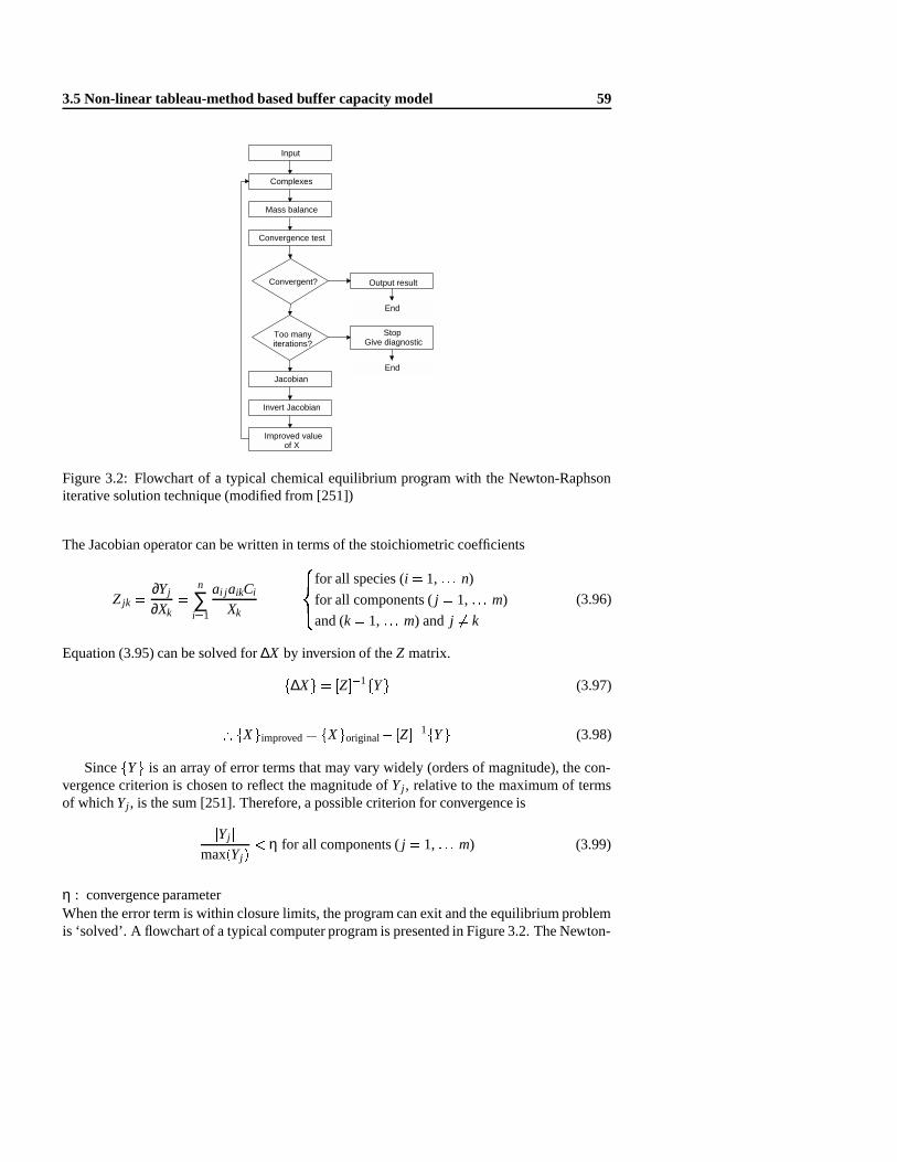
3.5 Non-linear tableau-method based buffer capacity model 59
Input
Complexes
Invert Jacobian
Convergence test
Mass balance
Improved valueof X
Output result
Jacobian
Convergent?
Too manyiterations?
StopGive diagnostic
End
End
Figure 3.2: Flowchart of a typical chemical equilibrium program with the Newton-Raphsoniterative solution technique (modified from [251])
The Jacobian operator can be written in terms of the stoichiometric coefficients
Zjk =∂Yj
∂Xk=
n
∑i=1
ai j aikCi
Xk
8><>:
for all species (i = 1, : : : n)
for all components (j = 1, : : : m)
and (k= 1, : : : m) and j 6= k
(3.96)
Equation (3.95) can be solved for∆X by inversion of theZ matrix.
f∆Xg= [Z]�1fYg (3.97)
) fXgimproved= fXgoriginal� [Z]�1fYg (3.98)
SincefYg is an array of error terms that may vary widely (orders of magnitude), the con-vergence criterion is chosen to reflect the magnitude ofYj , relative to the maximum of termsof whichYj , is the sum [251]. Therefore, a possible criterion for convergence is
jYj jmax(Yj)
< η for all components (j = 1, : : : m) (3.99)
η : convergence parameterWhen the error term is within closure limits, the program can exit and the equilibrium problemis ‘solved’. A flowchart of a typical computer program is presented in Figure 3.2. The Newton-

60 Mathematical pH buffer capacity modelling
Raphson method is one of the oldest and still most widely used numerical technique for solvinga set of nonlinear equations [262].
3.5.2 Precipitation and dissolution in equilibrium models
One of the powerful features of the tableau-based method for solving chemical problems is thepossibility to include precipitation and dissolution of species. From a chemical point of view,precipitation and dissolution reactions are conditional, they only occur if certain conditions(solubility product) are fulfilled. From a mathematical point of view, this means that suchreactions will introduce discontinuities in e.g. an algebraic model, or from a numerical pointof view the introduction ofif : : : thenstructures in the model. As a result of this, buffer capacitymodelling approaches presented in sections 3.3 and 3.4 cannot be used when one wants toinclude precipitation or dissolution reactions.
Chemical equilibrium models are quite structured in the manner that one designates precip-itation and dissolution of species. Several models [10, 198] use a format where each chemicalspecies is assigned a ‘Type’ upon data entry.
� Type I species – all the aqueous chemical species designated ascomponents.� Type II species – all other aqueous species not designated in Type I.� Type III species – all fixed species including solids designated to be present at chemical
equilibrium and not subject to complete dissolution.� Type IV species – all finite solids that are presumed to be present initially and have the
potential to be completely dissolved if the solution becomes undersaturated.� Type V species – all solids that may precipitate from solution but are presently under-
saturated.� Type VI species – all species that are excluded from mass balance calculations (e.g.
gases, electrons,: : : ).
The number of degrees of freedom of the chemical equilibrium problem is the number ofindependent variables. The Gibbs’ phase rule for computer modelling purposes is
F =C�P (3.100)
F : number of degrees of freedomC : number of chemical componentsP : number of Type III + Type IV species
By specifying Type III and Type IV species, we decrease the number of degrees of free-dom. As long asF is positive, the computer calculations will proceed. IfF is zero or less, adiagnostic will prompt the user to restructure the problem. To understand why Type III andType IV species decrease the number of degrees of freedom, consider the case of CaCO3(s)dissolution as a type IV solid.
CaCO3(s)Ca2++CO2�3 logKs0 =�8:42 (3.101)
As long as CaCO3(s) is present, the product of calcium ions and carbonate ions is fixed;they are not both independent variables, therefore we loose 1 degree of freedom. If carbonate

3.5 Non-linear tableau-method based buffer capacity model 61
anion increases, calcium ion must decrease.
[Ca2+] =10�8:42
[CO2�3 ]
(3.102)
3.5.3 Non-linear tableau-based buffer capacity model
The tableau-based method for solving chemical equilibria can be adapted and used for thesimulation of buffer capacity profiles. However, there are some slight modifications necessary.The available software is mainly focused on speciation calculations, and, although, the steptowards buffer capacity curve modelling is theoretically possible, it is not readily implementedin software like MINTEQA2 [10]. The following steps will be taken in order to develop atableau-based buffer capacity model:
1. According to sections 3.3 and 3.4, for mathematical and computational reasons, the ap-proach will be a ‘fixed pH approach’. Because the concentrations of thecomponentsareiteratively changed in the tableau-based method until a certain convergence is reached,[H+] is no longer a component, but will be treated as constant value, similar to theKvalues.
2. Because[H+] is kept fixed in the equilibrium calculations, the degrees of freedom canbe decreased with 1.
3. Leaving out[H+] as a component means also that the mass balance for this component(here, the charge balance) is not included in the iterative Newton-Raphson procedure.
4. If we assume titration with a strong base (e.g. NaOH), and the counter-ion (Na+ in thiscase) is assumed not to enter in any specified chemical reaction, the concentrationCB ispresent in only 1 equation, being the charge balance (cfr. example discussed in the set ofequations (3.78). For this reason, together with the previous point, it’s useless to includethe[Na+] with concentrationCB in the tableau.
5. When for a particular pH, the tableau method has found a chemical equilibrium solution,and found the concentrations for all species, the excluded charge balance will be usedto calculate the value ofCB, because all species in the charge balance will be known,except for[Na+] with concentrationCB.
6. OnceCB = f (pH) is established, the buffer capacityβ can be calculated. However theapproach forβ will be different from the approach in sections 3.3 and 3.4 because therelationship betweenCB and pH will be numerical in the tableau method, while it wasalgebraic or symbolic in the 2 previous approaches. In other words, the expression forβin equation (3.23) will be modified fromdCB
dpH to ∆CB∆pH.
To illustrate these six different steps to build a tableau-based buffer capacity model, thesame example of a solution containing phosphoric acid and Ca2+ of section 3.4 will be re-peated. The number of components for the approach of the conventional tableau-method wouldbe 3. But because we take a ‘fixed pH approach’, the number of independent components re-duces to 2. The components which are chosen preferentially are H3PO4 and Ca2+.

62 Mathematical pH buffer capacity modelling
Table 3.2: Species, components and stoichiometric information of the Ca2+�H3PO4 example
Components
Species H3PO4 Ca2+ H+ flogKgH3PO4 1 0 0 0H2PO�
4 1 0 �1 �2:2HPO2�
4 1 0 �2 �2:2�7:2PO3�
4 1 0 �3 �2:2�7:2�12:4Ca2+ 0 1 0 0CaH2PO+
4 1 1 �1 �2:2+1:4CaHPO0
4 1 1 �2 �2:2�7:2+2:7CaPO�4 1 1 �3 �2:2�7:2�12:4+6:5OH� 0 0 �1 �14
Ca CCa
The species, components and stoichiometric matrix information for this example is pre-sented in Table 3.2. Table 3.2 summarizes the equilibria and mass balances that were presentedin equations (3.69)�(3.76) and equation (3.25). Note that in order to write the species equilib-rium equations in function of the 2 components, substitutions of equations into other equationswas necessary in order to find the appropriateflogKg values. This is a mainly manual process,and it appears difficult to automate this for general purposes. For example, the equilibriumequation for CaH2PO+
4 is found by rewriting equations (3.69) and (3.72) respectively into:
log[CaH2PO+4 ] = log[H2PO�
4 ]+ log[Ca2+]+1:4 (3.103)
log[H2PO�4 ] = log[H3PO4]� log[H+]�2:2 (3.104)
followed by substitution of equation (3.104) into (3.103):
log[CaH2PO+4 ] = log[H3PO4]+ log[Ca2+]� log[H+]�2:2+1:4 (3.105)
The latter equation is formulated in the stoichiometric information matrix in Table 3.2. Thegeneral equation (3.90) of the tableau method needs to be extended here for buffer capacitycalculations with one term due to[H+] being excluded as a component:
fC�g= [A]fX�g+fBg log[H+]+fK�g (3.106)
fBg : column vector of stoichiometric H+ coefficients,n dimension

3.5 Non-linear tableau-method based buffer capacity model 63
Equation (3.106) together with equation (3.93) can now be solved for a particular chosenpH value with the iterative Newton-Raphson numerical solution technique, as illustrated insection 3.5.1. This will result in equilibrium concentrations for all considered species. Thebuffer capacityβ at the considered pH can be calculated with equation (3.23) if we know theconcentrationCB. CB can easily be found by rearranging equation (3.77), which was not useduntil this point.
CB = [H2PO�4 ]+2[HPO2�
4 ]+3[PO3�4 ]+ [CaPO�4 ]
+[OH�]� [H+]�2[Ca2+]� [CaH2PO+4 ] (3.107)
Unfortunately, the analytical approach of calculatingβ by taking the first derivative ofCB
towards pH, equation(3.79), cannot be taken here because the relationship betweenCB and pHis purely numerical in this tableau based approach. This forces us to use a numerical derivativeprocedure to findβ. Because of the high numerical precision that can be reached with modernsoftware and computers, a simple first derivative algorithm like the Euler algorithm will mostlysuffice.
β =dCB
dpH� ∆CB
∆pH=
CB(pH+∆pH)�CB(pH�∆pH)2∆pH
(3.108)
where∆pH is a sufficiently but not too small value, in order to obtain a correct value forβin function of pH. The illustrated example did not contain any precipitation or dissolutionreactions. However, a similar approach can be followed for systems with this kind of chemicalreactions. An extra step at the end of each iteration loop will have to be included. This will beillustrated with an example in section 3.5.5.
3.5.4 Ionic interaction effects
A similar ionic strength correction as presented for the general linear buffer capacity model(section 3.3.6) can be applied here too. The introduction of mixed acidity constantsK 0
a (seesection 2.2.4 on page 19) instead of acidity constantsKa, makes that all species can be writtenas concentrations, except for H+, that has to be written as an activity,fH+g. Because a pH me-ter delivers the H+ activity (see section 2.1 on page 5 and section 2.2.2 on page 15), the buffercapacity is expressed in function offH+g instead of[H+]. Subsequently, the stoichiometricinformation can be written in terms of concentrations for all species, and in terms of activityfor H+. However, as also noted in section 3.3.6, the mass balances and charge balance shouldbe written in terms of concentration. Therefore, the equation (3.107) has to be corrected:
CB = [H2PO�4 ]+2[HPO2�
4 ]+3[PO3�4 ]+ [CaPO�4 ]
+[OH�]� fH+gγH+
�2[Ca2+]� [CaH2PO+4 ] (3.109)
Summarized, and in general, ionic strength effects can be introduced in the tableau methodwhen the following steps are taken:
� Replace[H+] by fH+g in all equations.

64 Mathematical pH buffer capacity modelling
� UseK0a values instead ofKa values.
� Replace in the charge balancefH+g by fH+gγH+
.
3.5.5 Precipitation and dissolution in the tableau-based approach
The introduction of Type IV and Type V species (see section 3.5.2) into a chemical equi-librium model lead to mathematical discontinuities, which need a careful approach. If weconsider reaction (3.101), the corresponding equilibrium equation (3.102) is only valid as longas CaCO3(s) is present. When the solution becomes undersaturated, the equilibrium equation(3.102) is not valid any more and has to be eliminated from the model, for as long as thesolution stays undersaturated.
We will consider the example of section 3.5.3 of which the stoichiometric information ispresented in Table 3.2. We will consider a titration from low pH (e.g. pH= 4) until thepH where CaHPO4(s) with pKs0 = 6:66 starts to precipitate. Because the calculation of thebuffer capacity curve is based on simulations with increasing pH-values which are definedby the user, it is possible to verify at each simulated pH value if there is a possibility forprecipitation. This can be done by comparing the ion-product of the possible precipitate withthe solubility productKs0. In the example, Ca2+ and HPO2�
4 ions are present, so we canconsider a CaHPO4(s) precipitate.
CaHPO4(s)Ca2++HPO2�4 with pKs0 = 6:66 (3.110)
There will be no precipitation as long as[Ca2+] � [HPO2�4 ] < Ks0. From the moment the ion
product exceedsKs0, we need to take into consideration a new species, being CaHPO4(s).However, from a stoichiometric and mathematical point of view, this means that the completesystem has to be restructured.
As discussed in section 3.5.2, the number of degrees of freedom will decrease with 1 dueto the precipitate, so the amount of components also decreases with 1. Practically we willhave to set up a completely different stoichiometric matrix. The new species, components andstoichiometric matrix is presented in Table 3.3. The chemical equilibria presented in Table3.3 are the result of restructuring the original equations and write them all down in functionof H3PO4 and H+. The precipitated CaHPO4(s) is normally not considered as species becausewe cannot write down an equation expressing the concentration of precipitate. We need toconsider the precipitate to be present as long as the IAP of Ca2+ and HPO2�
4 is higher thanKs0. Often in chemical equilibria problems, solids are chosen as components if one wantsto calculate dissolution or precipitation amounts [251], but we didn’t need to do that for thisexample. The mass balance for the H3PO4 component is not straightforward, because anunknown concentration of HPO2�4 is precipitated with Ca2+. We can express that the amountof Ca2+ precipitated from the pool of calcium is equal to the amount of HPO2�
4 precipitatedfrom the pool of phosphorus.
CCa� [Ca2+]� [CaH2PO+4 ]� [CaHPO0
4]� [CaPO�4 ] =Ca� [H3PO4]
�[H2PO�4 ]� [HPO2�
4 ]� [PO3�4 ]� [CaH2PO+
4 ]� [CaHPO04]� [CaPO�4 ] (3.111)
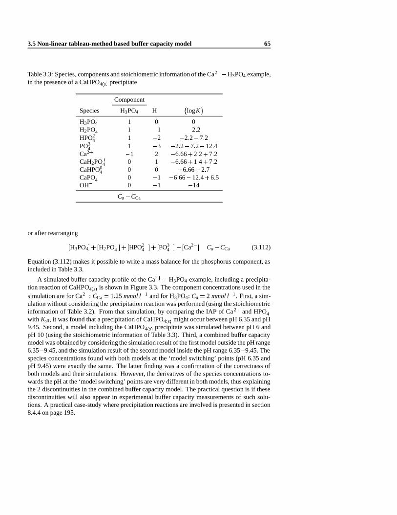
3.5 Non-linear tableau-method based buffer capacity model 65
Table 3.3: Species, components and stoichiometric information of the Ca2+�H3PO4 example,in the presence of a CaHPO4(s) precipitate
Component
Species H3PO4 H+ flogKgH3PO4 1 0 0H2PO�
4 1 �1 �2:2HPO2�
4 1 �2 �2:2�7:2PO3�
4 1 �3 �2:2�7:2�12:4Ca2+ �1 2 �6:66+2:2+7:2CaH2PO+
4 0 1 �6:66+1:4+7:2CaHPO0
4 0 0 �6:66+2:7CaPO�4 0 �1 �6:66�12:4+6:5OH� 0 �1 �14
Ca�CCa
or after rearranging
[H3PO4]+ [H2PO�4 ]+ [HPO2�
4 ]+ [PO3�4 ]� [Ca2+] =Ca�CCa (3.112)
Equation (3.112) makes it possible to write a mass balance for the phosphorus component, asincluded in Table 3.3.
A simulated buffer capacity profile of the Ca2+�H3PO4 example, including a precipita-tion reaction of CaHPO4(s) is shown in Figure 3.3. The component concentrations used in thesimulation are for Ca2+: CCa= 1:25mmol l�1 and for H3PO4: Ca = 2 mmol l�1. First, a sim-ulation without considering the precipitation reaction was performed (using the stoichiometricinformation of Table 3.2). From that simulation, by comparing the IAP of Ca2+ and HPO�4with Ks0, it was found that a precipitation of CaHPO4(s) might occur between pH 6.35 and pH9.45. Second, a model including the CaHPO4(s) precipitate was simulated between pH 6 andpH 10 (using the stoichiometric information of Table 3.3). Third, a combined buffer capacitymodel was obtained by considering the simulation result of the first model outside the pH range6.35�9.45, and the simulation result of the second model inside the pH range 6.35�9.45. Thespecies concentrations found with both models at the ‘model switching’ points (pH 6.35 andpH 9.45) were exactly the same. The latter finding was a confirmation of the correctness ofboth models and their simulations. However, the derivatives of the species concentrations to-wards the pH at the ‘model switching’ points are very different in both models, thus explainingthe 2 discontinuities in the combined buffer capacity model. The practical question is if thesediscontinuities will also appear in experimental buffer capacity measurements of such solu-tions. A practical case-study where precipitation reactions are involved is presented in section8.4.4 on page 195.
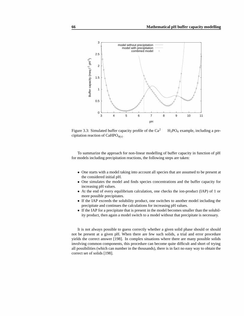
66 Mathematical pH buffer capacity modelling
0
0.5
1
1.5
2
2.5
3
3 4 5 6 7 8 9 10 11
Buf
fer
capa
city
(m
eq l-1
pH
-1)
pH
model without precipitationmodel with precipitation
combined model
Figure 3.3: Simulated buffer capacity profile of the Ca2+�H3PO4 example, including a pre-cipitation reaction of CaHPO4(s)
To summarize the approach for non-linear modelling of buffer capacity in function of pHfor models including precipitation reactions, the following steps are taken:
� One starts with a model taking into account all species that are assumed to be present atthe considered initial pH.
� One simulates the model and finds species concentrations and the buffer capacity forincreasing pH values.
� At the end of every equilibrium calculation, one checks the ion-product (IAP) of 1 ormore possible precipitates.
� If the IAP exceeds the solubility product, one switches to another model including theprecipitate and continues the calculations for increasing pH values.
� If the IAP for a precipitate that is present in the model becomes smaller than the solubil-ity product, then again a model switch to a model without that precipitate is necessary.
It is not always possible to guess correctly whether a given solid phase should or shouldnot be present at a given pH. When there are few such solids, a trial and error procedureyields the correct answer [198]. In complex situations where there are many possible solidsinvolving common components, this procedure can become quite difficult and short of tryingall possibilities (which can number in the thousands), there is in fact no easy way to obtain thecorrect set of solids [198].
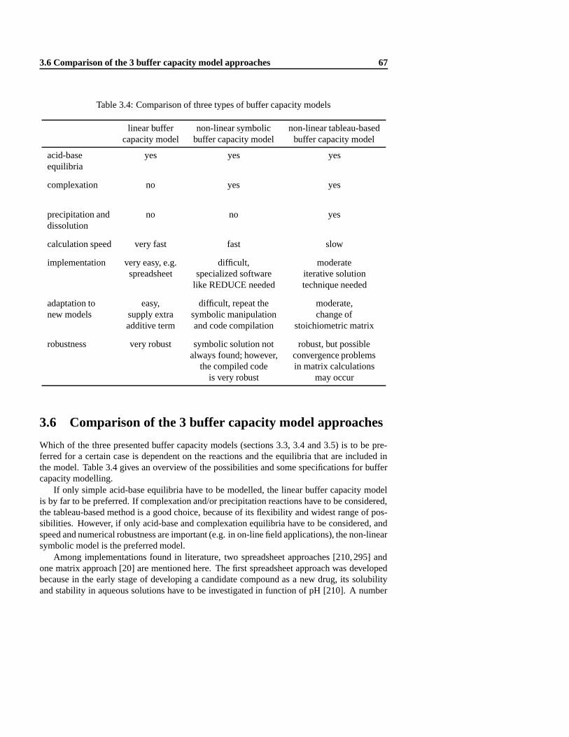
3.6 Comparison of the 3 buffer capacity model approaches 67
Table 3.4: Comparison of three types of buffer capacity models
linear buffer non-linear symbolic non-linear tableau-basedcapacity model buffer capacity model buffer capacity model
acid-base yes yes yesequilibria
complexation no yes yes
precipitation and no no yesdissolution
calculation speed very fast fast slow
implementation very easy, e.g. difficult, moderatespreadsheet specialized software iterative solution
like REDUCE needed technique needed
adaptation to easy, difficult, repeat the moderate,new models supply extra symbolic manipulation change of
additive term and code compilation stoichiometric matrix
robustness very robust symbolic solution not robust, but possiblealways found; however, convergence problems
the compiled code in matrix calculationsis very robust may occur
3.6 Comparison of the 3 buffer capacity model approaches
Which of the three presented buffer capacity models (sections 3.3, 3.4 and 3.5) is to be pre-ferred for a certain case is dependent on the reactions and the equilibria that are included inthe model. Table 3.4 gives an overview of the possibilities and some specifications for buffercapacity modelling.
If only simple acid-base equilibria have to be modelled, the linear buffer capacity modelis by far to be preferred. If complexation and/or precipitation reactions have to be considered,the tableau-based method is a good choice, because of its flexibility and widest range of pos-sibilities. However, if only acid-base and complexation equilibria have to be considered, andspeed and numerical robustness are important (e.g. in on-line field applications), the non-linearsymbolic model is the preferred model.
Among implementations found in literature, two spreadsheet approaches [210, 295] andone matrix approach [20] are mentioned here. The first spreadsheet approach was developedbecause in the early stage of developing a candidate compound as a new drug, its solubilityand stability in aqueous solutions have to be investigated in function of pH [210]. A number

68 Mathematical pH buffer capacity modelling
of methods and/or computer programs for calculation of solution pH and buffer capacity werereviewed by the authors, but these were found to be inconvenient for use in designing a buffersolution, since they ignore effects of ionic strength, do not involve effects of temperature, treatacids, bases and/or ampholytes separately, and eventually do not run on Windows which isnow widely used at workplaces. The developed program in Excel is useful for identifyingappropriate buffer solutions at various temperatures and/or ionic strengths [210]. The programis useful for prototyping, but not for simulations. One of the drawbacks for simulation appli-cations was found to be the limited possibility of Excel to deal with computational ‘loops’.The second spreadsheet application was developed for water conditioning purposes [295]. Theauthor points out that the main advantages of the use of spreadsheets for solving problems ofequilibrium chemistry are: its cheap implementation, the easy reuse, and the higher accessabil-ity for users. The disadvantage is that spreadsheets are limited to relatively simple problems.The developed spreadsheet could handle a number of topics related to the CO2�H2O system,like carbonate equilibria, construction of a lime titration curve, finding pH of a blend of twowater sources, calcium carbonate precipitation, and buffer capacity curves of inorganic carbonspecies [295].
For more complex problems in chemical equilibria, a set of FORTRAN routines (MAGIK)have been developed, which perform all of the necessary arithmetic for the solution of manytypes of complex equilibria [20]. It’s calculation engine is based on the Newton-Raphsonmethod of steepest descents (see also section 3.5), which is similar to packages presented be-fore like MINTEQA2 [10]. The main feature of the program is that it can handle titrations,contrary to many other programs, that can only handle single point equilibrium problems.More particular, MAGIK calculates species concentrations in function of a stepwise addedtitrant. The dynamic equilibria also include precipitation and dissolution. However, with achemical event such as precipitation, the concentration of one or more species will usuallysuffer an abrupt change, which is ultimately reflected as a mathematical discontinuity. Themathematical discontinuity is a situation in which not only specific variables will change dras-tically, but entire equations will no longer be valid. To overcome this problem, a possibilityto swap between 2 sets of equations was implemented in the software. A model swap is nec-essary when a precipitation reaction starts, or when the precipitate redissolves. These modelswaps must occur at the precise instant that both models overlap and where one supersedesthe other in order to get a smooth continuity of results [20]. The models and the model swap-ping condition have to be entered by the user in a subroutine, so that in case there are severalpossible precipitates/dissolutions, this approach will also be infeasible or impossible to im-plement. Eventually, off-line studies with several sets of models can help to determine whichprecipitation/dissolution reactions will occur first, and once the sequence of reactions is found,this sequence can be implemented in e.g. MAGIK [20] to obtain a full titration profile of thesystem. For each chemical equilibrium problem, a user-defined FORTRAN subroutine needsto be compiled and linked with the main program MAGIK. This is a serious drawback for fieldapplications, or in an automatic model building approach (see chapter 9).

Chapter 4
Field technologies for aquaticmonitoring
In this chapter, a literature review on technologies, practical experiences, relevance, problems,equipment, etc. related to the on-line measurements in activated sludge systems, rivers andother aquatic streams is presented. Because of the very broad range of existing technologiesand applications in this area, this literature study will only highlight these techniques andsensors for which the developed buffer capacity sensor in this work can be considered as apossible alternative. Taking this into account, the techniques that will be considered are chosenby the following criteria:
1. On-line or potential on-line application;
2. Application in wastewater effluent, river water, process water and other aquatic streams;
3. Measurement of chemical substances that directly or indirectly (after transformation intoanother chemical) induce a pH buffer capacity in the measurable range between pH 3and pH 11. More particular, ammonium, nitrate, phosphate, alkalinity and VFA’s areamong measurements that will be treated in this chapter;
4. Application measurement range in the order of magnitude of 0.1mmol l�1 for eachchemical substance. This is one of the main reasons that drinking water applications arenot discussed here, because in this area, the minimal measurable concentrations that arenecessary cannot be achieved with a buffer capacity based sensor.
Furthermore, the benefits of on-line measurements compared to off-line measurements ishighlighted in section 4.1. Existing sensors which are based on pH titration or buffer capacityprofiles will be discussed separately in section 4.4 because they can be of direct importanceto compare with the results obtained in this work. The goal of this chapter is to present aframework of existing sensors/methods, in order to make a positioning of the developed buffercapacity sensor into existing technologies.

70 Field technologies for aquatic monitoring
4.1 On-line measurement techniques
In the field of environmental measurements, in the last decades, one increasingly tries to imple-ment on-line measurements to replace off-line measurements. However, the results obtainedwith on-line measurements are sometimes unsuccessful. In cases where the expectations fromon-line measurements are high, and the difficulties related to these measurements are underesti-mated, installed on-line equipment will probably not produce the results as they were expected.This already highlights the difficulties and particularities related to on-line measurements.
The highest benefit of on-line measurements compared to off-line measurements is un-doubtedly the possibility to use this data for control purposes. In the field of biotechnologicalprocess control, better processing will come with the improvement of the biological knowl-edge and the application of automatic control [265]. In an ideal situation, the measured datashould be produced in-situ, on-line, continuously in real time and cover a wide dynamic rangein order to exploit them for process control. Aspects related to a successful implementation ofon-line sensors are discussed widely in literature [22, 127, 159, 161, 163, 265, 271, 332]. Theseaspects are related to the data reduction, database management [159, 265], data interpreta-tion [160, 161, 163], the human interface [265], maintenance and calibration related topics[161,332].
One of these application fields for on-line sensors that will be discussed in somewhat moredetails is the activated sludge wastewater treatment. The main objective of sewage treatmentwas previously to remove organic carbon compounds from the wastewater. However, the rangeof demands has greatly increased nowadays. Efforts now extend to complete elimination of ni-trogen and phosphorus [179]. At present, the most economical method for nitrogen removalseems to be biological nitrification-denitrification [26]. Until now chemical precipitation usingaluminium and iron salts and lime has been adopted in phosphate removal. However, this hasmajor disadvantages (large amount of chemicals, expensive, additional sludge,: : : ) and, con-sequently, biological phosphorus removal appears to be economically very attractive [26, 150].Alternating anaerobic/aerobic conditions of the biomass is one of the key factors triggeringoff phosphorus removal in excess of the normal assimilation (luxury uptake). The release ofo-PO4 in the anaerobic phase depends on several factors which can act separately or simulta-neously: e.g. the concentration of organic substrates and nitrates [109]. The alternating modeof operation involves that the concentrations of ammonium, nitrate and phosphate increaseand decrease periodically in the mixed liquor. By monitoring these dynamics with on-linemeasurements, the rates of nitrification, denitrification and phosphate uptake or release can bedetermined. This in turn provides valuable information for the understanding, modelling andon-line control of this process [18, 19, 128]. Besides on-line nutrient sensors for nitrate andammonium, ortho-phosphate and TOC, on-line alkalinity and turbidity measurements [256]are shown to be useful for process control purposes.
A major difficulty faced by plant operators in controlling the activated sludge process isthe inability to adequately monitor the process [271]. However, nowadays on-line sensors fordissolved oxygen, suspended solids, pH, temperature and flow are found accurate enough forcontrol purposes, under the conditions of correct use, frequent maintenance and calibrationetc. Today almost all plants are equipped with some of these sensors. A more interestingrange of instruments related to this work are the on-line nutrient sensors (e.g. ammonium,nitrate, phosphate). These sensors get a lot of attention nowadays and a lot of research and

4.1 On-line measurement techniques 71
commercialisation efforts are focused on this category of sensors. These sensors are expensiveequipment, but the benefits of these sensors can be very high, as will be illustrated with someexamples below.
On-line analyzers to monitor the effluent levels of ammonia and phosphate have been usedfor operational control of 4 nutrient removal activated sludge plants in Johannesburg [166].Savings of 1 million US dollar per year in the purchase of phosphate precipitation chemicalshave been achieved. Other authors point out two major obstacles to be considered with on-line nutrient sensors: First, that on-line measurements of ammonium, nitrate and phosphateare too unstable to be used for on-line control; Second, that no efficient control strategies aredocumented in the literature [291]. However, studies at several plants in Denmark have shownthat obstacle 1 is now overcome as these measurements are now used for direct control [291].The same study also showed that a responsible maintenance and surveillance is the key factor.Closed loop control strategies have been found efficient and robust for practical implemen-tation, and are economically favourable at most large plants with biological nutrient removal[291]. Another key factor is sample preparation. In order to obtain nutrient measurements inthe mixed liquor, most on-line apparatus need an extra membrane filtration step, because themeasurements would be disturbed by clogging in the small tubes of the nitrogen and phospho-rus monitors [292].
Data of on-line analyzers allow also up-to-date simulation using mathematical models ofthe treatment system [57, 213]. It is shown that computer simulation is a very powerful toolfor the optimization of the operation of wastewater treatment plants. Considering the bene-fits of computer simulation for plant operation, it is worth its price for medium to very largewastewater treatment plants [213]. The benefits from computer simulation are e.g. savingsin energy and chemical consumption [347], a decrease of nutrient levels in the effluent [292],and an increase of capacity of the plant [55, 56, 290]. An important point when designingand implementing a control system for wastewater treatment purposes is to make the controlsystem as simple as possible [347]. This includes the usage of simple control laws and fewsensors, which reduces the implementation and maintenance cost of the control system. Themost recent studies give promising results of upgrading treatment plants to N and/or P removalusing on-line sensors and appropriate control strategies [55, 266]. A Danish study on 14 treat-ment plants has shown that the introduction of control systems based on on-line sensors forammonia, nitrate and phosphate has resulted in a more stable effluent quality and an increasedcapacity [266]. This study also concludes that it may be better to incorporate a considerableflexibility into the design, allowing the processes to be adjusted to the time-varying operationalconditions. In another study, a simulation supported scenario analysis for the upgrading of amunicipal wastewater treatment plant was used [55]. A comparison was made between extend-ing the plant with new reactors, or re-design the existing reactors for increased performance.It was found that the most cost-effective solution was to create optimal aerobic and anoxicconditions within existing reactor volumes [55].
Despite all advantageous aspects concerning the benefits of on-line sensors, still many dif-ficulties and wrong measurements are noticed in practical use of on-line sensors. Instrumentfaults are to blame for many control problems and plant upsets, but the actual culprits often arehard to identify or are completely overlooked [246]. Unfortunately, most sensor errors maygo unrecognised, particularly if those signals are used in feedback control loops. Some typicalcauses of errors are: wrong sensor application, transmitter not properly calibrated, signal drift,

72 Field technologies for aquatic monitoring
electrical problems of wiring, shielding, grounding,: : : [246]. Another particularity related toon-line measurements for control purposes is the limitation of the measurement range of thesensors. E.g. typical values for nitrate used as set-point in the control strategy are around 1mgN l�1. The problem with this form of control is the inaccuracy of nitrate measurements inthe lower measuring range, i.e. the range used for the controlling variable. Frequent recalibra-tion and high maintenance efforts are required in such cases [164].
As the instrumentation systems become more complex, it becomes less satisfactory to dealseparately with designers, instrument manufacturers, information transfer specialists and oper-ators [334]. As a consequence of this there is e.g. a lack of process knowledge with instrumentdevelopers which can result in measurement systems which are very expensive but quicklybecome non-functional and mistrusted by operators [334]. Maintenance has always been oneof the most important functions of wastewater treatment operation. The increasing complex-ity of treatment, required standards and necessary control systems with the resultant possibleheavy costs make proper maintenance increasingly important [334]. On the one hand, on-lineanalyzer companies often suggest maintenance intervals of 1 week, or even 1 month, but onthe other hand practical field studies show that for complicated on-line sensors (e.g. N andP analyzers), a daily inspection should be carried out with all on-line analyzers [250]. Thisinspection can vary from a visual inspection to a full cleaning and calibration. In general, 20minutes per instrument and per day, including sample pre-treatment, are to be expected [250].
On-line measurements undoubtedly offer high benefits compared to off-line measurements,however, on-line measurements may not be considered as straightforward measurements. Thesuccessful use of on-line sensors does not only depend on the sensor itself, but also, and oftenmost importantly, on the process conditions, the sample preparation, the maintenance, cali-bration,: : : On-line sensor development is a challenging field for researchers because of thesemany aspects related to on-line measurements. The next section will present a number ofsensors that are related to the results of this work, being the nutrient sensors.
4.2 Nutrient sensors: State of the art
The aim of this section is to present the current situation of existing nutrient sensors for on-line environmental applications. More particular, sensors for ammonium, nitrite/nitrate andortho-phosphate will be presented. Besides the measurement principle, attention will focuson accuracy, precision, stability, maintenance requirements and common problems. Basically,the on-line analyzers make use of known laboratory measuring principles [307]. However,it is important to note that the measuring principles have often been modified (=simplified)compared to the standard laboratory method when applied to on-line analyzers [87].
4.2.1 Sample filtration
Most NH+4 , NO�
3 and PO3�4 -analyzers require a sample stream free of suspended solids, which
necessitates the use of a membrane filter sampling system [87, 250, 288, 289, 317]. Up to 46 %of the investment costs for the installation of an on-line analyzer can be due to the installationof a sampling and filtration system [250].

4.2 Nutrient sensors: State of the art 73
Figure 4.1: Diagram of a typical ultrafiltration (UF) module [89]
The sampling system is a crucial part of the measurement system. An ultrafiltration cross-filter system fed with a submerged shredding pump has been evaluated as being the most ap-propriate filter in activated sludge (influent, reactor, effluent) applications [220, 250, 288, 289,317]. The membrane filtration is carried out by means of a cross-flow filter in which a largemain flow (severalm3 h�1) is pumped vertically through the filter thus allowing a small sub-flow (approximately 3l h�1 to pass horizontally through the filter membrane. The unfilteredwastewater is returned to the plant/river. The filtered sample is distributed to the on-line meters[288, 289]. The high flow and the resulting shear forces prevent the deposit of small particleson the membrane surface [289].
In the past, other filter systems, like dialysis [220], a gauze filter equipped with a compres-sor for cleaning purposes [261], or smaller filter systems [289] have been tested but they oftensuffer from limited lifetime or clogging problems. Possible problems are case dependent (e.g.influent versus effluent). A schematic presentation of a typical sampling system is given inFigure 4.1. In practice, a set-up with two parallel ultrafiltration (UF) units (Figure 4.1) offersthe possibility to maintain a continuous sample flow to the analyzers [87, 317]. Built-in filtrateflow meters or pressure drop meters can automatically switch off the active unit and activate thespare one. Another filter control system consists of an electronic permeate weighing system,for early clogging detection [105].
The self cleaning power of the filtration unit is mostly not sufficient for continuous oper-ation. Therefore, cleaning with chemicals may be necessary at periodic intervals [250]. Au-tomatic cleaning can be obtained by an air blow or a hypochlorite chemical treatment [317].The manual maintenance frequency for an UF unit (e.g. manual cleaning) can vary from 1 dayfor wastewater influent to 2� 6 weeks for an effluent type of water [250]. The lifetime of a

74 Field technologies for aquatic monitoring
cross filter is typically 1 year [289]. The additional response time introduced by an UF unitcan vary between 3 and 20 minutes [288,289]. Typical technical problems that occur whenon-line filtration is implemented, are discussed in [96]. The authors have based their resultson a case study of a newly developed on-line river water measurement station, and concludethat considerable time is needed for the testing, calibrating, site-adaptation,: : : before reliablemeasurements can be obtained. Similar experiences were also obtained in [41, 96].
To overcome the difficulties related to sample filtration, recently on-line colorimetric sen-sors without need for a separate sampling and filtration unit have been developed [171]. Suchdevices are constructed as completely closed small containers, that are directly placed in e.g.the activated sludge aeration tank. The innovative part of this type of sensor is the particularmembrane that contacts the sludge. The membrane functions as an ion sieve with, in practice,no mass transportation of water. The thickness of the membrane is 50µmand the molecularweight cut-off of the membrane is approximately 100 Daltons. The lifetime of the membraneis tested to be well over one month, and no fouling of the membrane was observed [171]. Theprototype sensors are believed to have a big potential for further refinement, and the authorssuggest that the use of the sensors can be extended into other areas such as monitoring ofreceiving waters, sewer and drinking water systems [171]. However, no practical results inthese areas are available yet. Also, the announced commercialisation within wastewater treat-ment operation has not been established, which make us believe the initial reports were toooptimistic.
4.2.2 Ammonium analyzers
On-line ammonium analysis is mostly performed with a potentiometric (gas electrode) or acolorimetric method.
In the potentiometric or electrochemical method, the pH in the sample is raised above 11,thus converting all NH+4 to NH3. The NH3 is then measured by means of an NH3 gas sen-sitive electrode [289]. The gas electrode based ammonium analyzers are shown to have thewidest measuring range (0.1�1000mgN l�1)[250], and the shortest response time (less than8 minutes) [175, 250, 289]. Tests in nutrient removal activated sludge plants have shown thatthe electrochemical method is the more accurate and reliable [289], has the lowest reagentexpenses [289] and is free of interfering ions [175, 289, 326]. A disadvantage is that somecommercial electrode monitors lack temperature compensation capabilities [289, 326]. Someother reported problems include air building up under the electrode tip and electrode drift-ing [11]. Electrochemical methods perform better in effluents than in influents, because ofthe lower demand of chemicals and lower maintenance needs in effluents [165]. A recent de-velopment is the measurement of ammonia with a fibre optical analogue of the conventionalelectrochemical ammonia electrode [103]. Despite that no field experiences are available yet,the authors anticipate that many positive developments in this field are to be expected in theyears to come.
Colorimetric flow injection analysis (FIA) is most frequently applied for the analysis ofammonia in a diverse range of liquid samples, including those using the Berthelot reaction, inwhich ammonia reacts with phenol and hypochlorite to produce indophenol blue, and those us-ing Nessler’s reagent to form a yellow azo dye [14]. The higher chemical reagent consumption[289], the slower response time (5 to 20 minutes) [250], the sensitivity to temperature variation
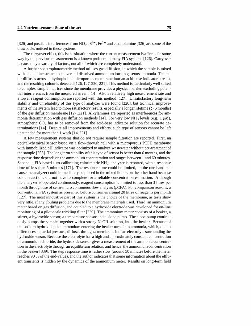
4.2 Nutrient sensors: State of the art 75
[326] and possible interferences from NO�2 , S2�, Fe3+ and ethanolamine [326] are some of the
drawbacks noticed in these systems.The carryover effect, this is the situation where the current measurement is affected in some
way by the previous measurement is a known problem in many FIA systems [126]. Carryoveris caused by a variety of factors, not all of which are completely understood.
A further spectrophotometric method utilises gas diffusion, in which the sample is mixedwith an alkaline stream to convert all dissolved ammonium ions to gaseous ammonia. The lat-ter diffuses across a hydrophobic microporous membrane into an acid-base indicator stream,and the resulting colour is detected [126,127, 220, 221]. This method is particularly well suitedto complex sample matrices since the membrane provides a physical barrier, excluding poten-tial interferences from the measured stream [14]. Also a relatively high measurement rate anda lower reagent consumption are reported with this method [127]. Unsatisfactory long-termstability and unreliability of this type of analyzer were found [220], but technical improve-ments of the system lead to more satisfactory results, especially a longer lifetime (> 6 months)of the gas diffusion membrane [127, 221]. Alkylamines are reported as interferences for am-monia determination with gas diffusion methods [14]. For very low NH3 levels (e.g. 1µM),atmospheric CO2 has to be removed from the acid-base indicator solution for accurate de-terminations [14]. Despite all improvements and efforts, such type of sensors cannot be leftunattended for more than 1 week [14, 221].
A few measurement systems that do not require sample filtration are reported. First, anoptical-chemical sensor based on a flow-through cell with a microporous PTFE membranewith immobilized pH indicator was optimized to analyze wastewater without pre-treatment ofthe sample [255]. The long term stability of this type of sensor is better than 6 months, and theresponse time depends on the ammonium concentration and ranges between 1 and 60 minutes.Second, a FIA based auto-calibrating colorimetric NH+
4 analyzer is reported, with a responsetime of less than 5 minutes [171]. The response time could be limited, on the one hand be-cause the analyzer could immediately be placed in the mixed liquor, on the other hand becausecolour reactions did not have to complete for a reliable concentration estimation. Althoughthe analyzer is operated continuously, reagent consumption is limited to less than 3 litres permonth through use of semi-micro continuous flow analysis (µCFA). For comparison reasons, aconventional FIA system as presented before consumes around 20 litres of reagents per month[127]. The most innovative part of this system is the choice of the membrane, as tests showvery little, if any, fouling problems due to the membrane materials used. Third, an ammoniummeter based on gas diffusion, and coupled to a hydroxide electrode was developed for on-linemonitoring of a pilot-scale trickling filter [339]. The ammonium meter consists of a beaker, astirrer, a hydroxide sensor, a temperature sensor and a slope pump. The slope pump continu-ously pumps the sample, together with a strong NaOH solution, into the beaker. Because ofthe sodium hydroxide, the ammonium entering the beaker turns into ammonia, which, due todifferences in partial pressure, diffuses through a membrane into an electrolyte surrounding thehydroxide sensor. Because the electrolyte has a high and approximately constant concentrationof ammonium chloride, the hydroxide sensor gives a measurement of the ammonia concentra-tion in the electrolyte through an equilibrium relation, and hence, the ammonium concentrationin the beaker [339]. The step response time is rather slow (around 50 minutes before the meterreaches 90 % of the end-value), and the author indicates that some information about the efflu-ent transients is hidden by the dynamics of the ammonium meter. Results on long-term field

76 Field technologies for aquatic monitoring
Table 4.1: Comparison of different on-line ammonium analyzers
Principle Ref. Detection Range Accuracy R.s.d. Maintenance Responselimit interval time
(mgNH+4 -N l�1) (%) (%) (weeks) (min.)
NH3 sensitive [289] 0.5�10 +4 8 1 10�15electrode [11] > 1 �28 to+178 40�120 1 10�15
[288] 0�12 �4 to�20 12�33 1[165] 0�100 < 1[326] 0.05�0.2 0�20000 1�14 1 6�12
FIA [288] 0�10 �7 to+3 2�32 1[165] 0�80 1�4[326] 0.17�0.9 0�100 0.7�18 1�4 2�21
FIA + GD unit [126] 0.5�50 1[14] 0.6 1�100 �15 1�5 1 30
optical/chemical [255] 0.01 0�14 9 1�60(no filtration)µCFA [171] 0.1 0�25 �5 3 4 < 5
experience of this type of sensor are not reported yet.Alternative methods for ammonium measurement, but at this moment only used in labora-
tory off-line analysis include a multi-component determination in which chloride and ammoniaare determined in the same sample with a single FIA system [306]; a centrifugal ammonia an-alyzer [186]; laboratory FIA systems based on the Berthelot reaction [232]; salicylate andenzymatic methods [143]. Typically these methods have low detection limits in the order ofmagnitude 1�50µgN l�1, but are not (yet) suited for on-line applications.
Comparison results of field studies with different types of ammonium sensors are presentedin Table 4.1. It can be seen that the reported values for detection limit, range, accuracy and re-peatability vary very much depending on measurement principle and the particular case study.
A detailed field test with 9 commercial ammonium sensors on the same location reporteddifferences of more than 200 % between measurements performed by the different sensorsunder test [326]. This is illustrated in Figure 4.2. An important offset difference betweendifferent sensors was noticed. The main concern was that some monitors often failed andneeded extra intervention and cleaning, multiple trials of calibration, changing of plastic pipesor other parts,: : : This field test has shown that every detail is important when installing andrunning a monitor. Particularly the filtration unit and piping are among the high maintenanceparts.
4.2.3 Nitrate analyzers
Numerous methods have been proposed for the determination of nitrate. Commercial on-line nitrate sensors are mainly based on ion-selective electrodes, colorimetric reactions or UVabsorption. Due to many interferences of other chemical species, alternative systems have been

4.2 Nutrient sensors: State of the art 77
Figure 4.2: Field test of NH+4 monitors [326]
developed for specific purposes. However the latter are often not commercialised as on-linesensor. Some of these ‘alternatives’ will be discussed here too.
The analyzers based on UV absorption are considered to be the best choice for field-use[87, 261, 289]. The advantages of this type of sensor are: A short response time (10 sec-onds), low maintenance needs and no need for chemicals [261,289]. Due to interference ofparticles with the UV absorption measurement, an ultra filter is needed for reliable operation[261]. Nitrate and nitrite are measured together, as they both absorb UV at 210nm [269]. Acalibration frequency of only once in 6 months can be sufficient [261], but in some applica-tions UV absorption NO�3 analyzers were reported to have a moving baseline, which couldbe solved by a frequent automatic zero calibration [11]. In some applications, interferencesof UV-absorbing organic matter (e.g. aromatic compounds) may influence the measurements[11, 165, 269, 288, 289]. A possible solution is the dual wavelength approach, where the strongabsorbance of nitrate in the 210nm region is measured relative to the absorbance in a regionwhere nitrate does not absorb. The wavelength 275nmcan be used to compensate for mainlyorganic interferences [104,269].
The electrochemical meters based on an ion-selective NO�3 -electrode are good because
of their low pre-treatment demand resulting in a short response time (less than 10 minutes),and their low chemical consumption [250, 289]. However the nitrate electrode is sensitive toelectrode drift [221], disturbing ions (e.g. HCO�3 ) and fouling of the electrode [261]. Chlorideand bicarbonate ions interfere when their weight ratios to NO�
3 -N are> 10 or> 5, respectively[104]. Erratic responses have been noted when the pH and ionic strength are not held constant

78 Field technologies for aquatic monitoring
in all samples and standards [104]. Another drawback of this system is the limited lifetime(2�3 months) of the expensive electrodes [261]. Sample pre-treatment, frequent automaticcalibration (including pH and ionic strength corrections) and availability of a spare electrodecan partly alleviate such problems [87].
Colorimetric NO�3 analyzers are considered to be the most accurate [165], but also have thehighest maintenance needs, making them less favourable for field-use. Some studies illustratethat these sensors are sometimes too unreliable for use as process equipment in situations whereseveral days unsupervised operation is necessary [220, 289]. Colorimetric sensors first convertNO�
3 to NO�2 . This reduction step can either be done with a Cd column [126, 220, 288, 289]
or with hydrazine [104, 171, 288]. In the following step, a yellow or red azo-dye which can bemeasured optically is formed with NO�2 . In such a way NO�2 eventually present in the sampleis measured together with NO�3 . The installation of two injection valves, one before and oneafter the Cd column, results in a double peak, which can be associated with nitrate and thesum of nitrate and nitrite [165, 221]. In order to minimize the analyzer complexity, it is notworthwhile to include this extra step in cases where NO�
2 is normally quite low [126]. Some ofthe problems of the unreliability in the field can be related to the Cd column. Suspended mattercan restrict the sample flow, oil and grease will coat the Cd column, reducing its efficiency[104]. A reliable sensor, without filtration needs was realised by placing the analyzer directlyin the measurement stream (e.g. mixed liquor) and using a membrane device that functions asan ion sieve [171] (see also section 4.2.1).
Another type of NO�3 analyzer is a flow-injection analysis system with an amperometricdetection system [269]. Nitrate is determined as nitrite after reduction in a Cd column. Theworking electrode is glassy carbon modified with a crosslinked redox polymer. Its main ad-vantages are twofold; first of all no sample pre-treatment is needed and fast sample throughputis possible. Secondly, with this measurement technique the effect of interferences is reducedconsiderably since only species with an appropriate redox potential are detected with thesepolymer modified electrodes. Only nitrite and iron could possibly interfere in the reductionprocess [269]. At this stage the sensor has been designed for the laboratory environment only.
Other continuous flow methods, but so far only used off-line, use titanium(III)chloride asreducing agent for NO�3 [9, 15]. Nitrate can be reduced to nitrite with TiCl3, and determinedspectrophotometrically as usual [9], or it can be reduced to ammonia in alkaline medium byTiCl3 [15]. In the latter method, the interference of nitrite initially present in the sample can bemasked with sulfonilic acid. A NH3 determination before and after the reduction step makesa simultaneous determination of nitrate and ammonium possible. The detection limits of thesemethods are between 3 and 20µgNO�
3 -N l�1. Despite the fact that from a technical point ofview, these methods are not more complicated than e.g. the Cd reduction method, no exampleswere found where this principle is implemented as on-line sensor.
The usual reducing agents for NO�3 are not sufficiently specific and it is normally difficultto obtain a quantitative reduction of nitrate to nitrite [34]. Methods based on enzymatic orbacterial reduction of nitrate are assumed to be more specific [34] and free from interferences[136]. However, a possible drawback and reason why these methods are not found in com-mercial sensors, is the necessity to have specialised personnel for the preparation/handling anduse of enzymatic or bacterial suspensions. Consequently, such methods are typically foundin laboratory environments instead of in the field. Although in special cases (e.g. carboniza-tion wastewater), where commercial available on-line nitrate sensors were not suitable due

4.2 Nutrient sensors: State of the art 79
to interferences, an on-line FIA system including a biological nitrate to nitrite reduction us-ing immobilizedE. coli cells combined with selective nitrite determination was implemented[196].
Basically there are two different approaches to the biological conversion of nitrate. First,there are the enzymatic methods, where the enzyme is used in purified or unpurified form (in-cluding other cell material); the enzyme can be immobilised in pellets or kept in suspension.Second, living cell methods exist where the biological nitrate conversion is mostly obtainedwith a specific bacterial strain. The latter method offers some advantages like: an increasedelectrode lifetime, regeneration of electrode response, and the elimination of tedious, time-consuming enzyme isolation and purification steps [140]. The use of bacteria would be par-ticularly superior for systems in which more than one enzymatic step along with cofactors arerequired to produce the measured product [140]. A disadvantage of living cell sensors is theirhigher sensitivity for toxic substances in the measurement solution.
Enzymatic methods which reduce nitrate into nitrite using nitrate reductase were reportedby [34, 137, 167, 196, 342]. The nitrite formed can be measured by a standard diazoting colori-metric method [34, 167, 196] or by fluorometric detection in which NADH is used as electrondonor [137]. In these methods special care has to be taken that NO�
2 is not further reducedto N2O etc. [167]. The detection limit of these methods is around 10�50 µgNO�
3 -N l�1 inlaboratory conditions [137, 167]. An on-line sensor using this method [196], in which bacterialE. coli cells were immobilized in spherical alginate beads with diameter 4�5 mmobtained alower sensitivity compared to other commercial available instruments. The detection limit wasaround 1mgNO�
3 -N l�1, which is still sufficient for most monitoring purposes. The sensorused a built-in continuous data correction to compensate for activity loss of the biologicallycatalysed reduction process [196].
An enzymatic sensor in which nitrate was reduced to nitrite (using nitrate reductase), fol-lowed by a second reduction step to ammonia (using nitrite reductase) overcame the problemthat the colorimetric NO�2 measurement method is rather complicated [136]. The ammoniaproduced is monitored, using an air-gap ion-selective electrode. A measurement range be-tween 0.7 and 140mgNO�
3 -N l�1 was obtained [136].A novel approach to the development of bioselective sensors has been the use of intact bac-
terial cells in place of isolated enzymes at the surface of a membrane electrode [140]. A poten-tiometric sensor has been devised for nitrate by coupling the bacteriumAzotobacter vinelandiiwith an ammonia gas sensing electrode [140]. The response of this sensor was found to belinear over the concentration range 0.1 to 10mgNO�
3 -N l�1. The electrode was useful for aperiod up to two weeks. The bacterial electrode must be stored in growth medium when not inuse. Another type of microbial NO�3 -electrode consists of immobilisedPseudomonas aerugi-nosaand a carbon dioxide gas-sensing probe [114]. In this system nitrate was determined bymeasuring carbon dioxide with a gas sensing probe under anaerobic conditions accompanyingan excess carbon source, ethanol in this case [114]. As carbonate interfered with the determi-nation, pre-treatment was made to remove CO2 by adjusting the pH of the sample at 4.0 andbubbling with nitrogen gas for 1 minute. The electrode was tested on samples from a wastew-ater treatment plant. The cycle time for 1 measurement was 30 minutes and the response waslinear between 5 and 50mgNO�
3 -N l�1.On-line analyzers for total nitrogen also become available [73, 141, 250]. The measurement
principle of these sensors can be based on the hot catalytic conversion of bonded nitrogen to

80 Field technologies for aquatic monitoring
Table 4.2: Comparison of different on-line and semi on-line‡ nitrate analyzers
Principle Ref. Detection Range Accuracy R.s.d. Maintenance Responselimit interval time
(mgNO�
3 -N l�1) (%) (%) (weeks) (min.)
UV absorption [250] 0.1�100 < 5[288] 0�5 �3 to+260 5�20 1[165] 0�50[289] 1�7 < 0:5 4 4 3�9[11] +47 32 1
[269]‡ 0.4 0.4�30 2�4 1.7NO�
3 selective [288] 0�10 �1 15 1electrodeColorimetric [288] 0.5�7 �10 20�24 1with Cd [165] 0�50 1 20
[126] 0.5�20 1[218] 0.1 0�4 �3 < 1[156] 1 0�25
Colorimetric [22, 171] 0.07 0�10 �10 5 4 5with hydrazineEnzymatic [196] 1NO�
3 ! NO�
2
nitrogen monoxide [250] or on in-line UV catalysed oxidation of organic nitrogen to nitrate,which is measured colorimetrically [73]. The latter method found recoveries of different ni-trogen forms between 90 and 100 %. However comprehensive practical experience is not yetavailable [250].
A comparative literature review on different nitrate analyzers is presented in Table 4.2.
4.2.4 Phosphate analyzers
The majority of on-line phosphate sensors are colorimetric methods, thus requiring a filtra-tion unit prior to the analyzer unit. As a consequence of the fact that no phosphate selectiveelectrode is available, often FIA methods are chosen for this measurement [221]. Phosphatecan either be determined as ortho-phosphate or as total phosphate. Total phosphate analysisrequires more manipulations because phosphorus compounds must be decomposed into ortho-phosphate.
Two colorimetric ortho-phosphate analysis methods are employed: the molybdenum bluemethod and the vanado-molybdate method [250]. The molybdenum blue complex is formedby the reduction of the reaction product between ortho-phosphate and ammonium molyb-date. The reducing agents that can be used include ascorbic acid [288] and stannous chloride(Tin(II)chloride) [32]. Some reducing agents are reported to have a limited lifetime so that thereagent autonomy is reduced to maximum 1 week [220]. Tin(II)chloride as reductant makesthat the wavelength maxima of the blue complex are at 690�700nmcompared with 882nmfor ascorbic acid. This offers the advantage of greater sensitivity when a solid state detector

4.3 Developments in effluent and river water monitoring 81
which uses a red light-emitting diode light source (λmax� 635nm) is used [32]. Similar to themolybdenum blue method, the vanado-molybdate method also starts with a reaction betweenortho-phosphate and ammonium molybdate to form molybdophosphoric acid. In the pres-ence of vanadium, yellow vanado-molybdophosphoric acid is formed [104]. This compoundis measured photometrically at a wavelength of usually 470nm.
Field studies have shown that automatic ortho-phosphate analyzers are more stable andreliable than ammonium or nitrate analyzers, mainly because no membranes and columns areneeded [220]. The chemical expenses for ortho-phosphate determinations are very high whichis, however, to some degree balanced by a low purchase price [289]. More recent studies [288]show that phosphate analyzers have been optimized in the last 5 years, so that its operatingcost is nowadays comparable with the operating costs of ammonium and nitrate analyzers.
Despite all technical improvements and longer autonomy of the analyzers noticed in thelast years, the weakest part of the measurement chain remains the filter system [33]. Further,the molybdenum blue colour complex can give precipitation problems on the inner walls of thetransport tubes and on the detector’s flow cell windows [126]. In such situations more frequentmanual cleaning (e.g. 0.5M HCl) is advised. The use of ascorbic acid as reductant for themolybdenum blue complex was found to be unaffected by the presence of organic phosphates,pyrophosphates and polyphosphates [39].
Besides colorimetric measurement systems, other methods are available too, like the com-bined enzymatic and amperometric FIA biosensor system [174]. This sensor contains twoimmobilised enzymes (nucleoside phosphorylase and xanthine oxidase). In a laboratory set-up, response times were less than 6 minutes. However, no on-line results with this sensor areavailable [174].
In water and wastewater systems, total phosphorus (TP) concentration is commonly usedas an indicator of water quality and as control parameter in wastewater treatment processes.On-line techniques for TP are available [30, 73, 141]. They are based on a colorimetric mea-surement of ortho-phosphate after a destruction of TP into ortho-P. The methods differ in theway the on-line destruction step is performed. Polyphosphates can be hydrolysed with acid andheat, while organophosphates can be digested with UV-catalysed persulfate oxidation [73].Others use nitric-sulphuric acid, perchloric acid or potassium peroxodisulphate as oxidisingagent [31, 141], eventually at high temperature and pressure. Other on-line digestion systemsinclude a flow-through reactor in a modified microwave oven [30] or a combined UV/thermalinduced digestion [31, 73]. The latter method can be used without sample pre-treatment priorto analysis. For separate determinations of ortho- and polyphosphates, no on-line method is re-ported, but rapid laboratory methods like anion exchange chromatography are available [132].
A comparative study of different phosphate analyzers is presented in Table 4.3. The ac-curacy and repeatability of phosphate analyzers is better than for ammonium and nitrate ana-lyzers. This can possibly be due to less interferences in the phosphate colorimetric reactions.
4.3 Developments in effluent and river water monitoring
The detection of accidental discharges of pollutants in effluents and river waters is importantto get more insight in the sources of pollution and take the necessary control actions. In this

82 Field technologies for aquatic monitoring
Table 4.3: Comparison of different on-line phosphate analyzers
Principle Ref. Detection Range Accuracy R.s.d. Maintenance Responselimit interval time
(mgPl�1) (%) (%) (weeks) (min.)
Colorimetric [22, 171] 0.2 0�10 �5 3 4 5molybdenum [126, 220] 0.5�50 1blue [250] 0.01�5 < 12
[288] 0.2�4 �1 to+23 5 1[165] variable 1 20
[32, 33] 0.05 0�25 �2:5 0.4 > 1Colorimetric [289] 0.05�1 �1 4 1 8�13vanado- [11] 3 9 1molybdate [250] 0.1�20 <12
[288] 0�4 �4 to+40 8�13 1[165] 0�15 > 1[156] 0.3 0�25
TP (including [30] 0.09 0�18 �(1�30) 2digestion step) [31] 0.15 0�18 �(1�20) 1
section, a number of methods and sensors are presented that can be used for alarm generatingpurposes. Most of the presented sensors are on-line systems, measuring non-specific sub-stances. Special attention is given to UV based sensors, because their application area is mostsimilar to the developed buffer capacity based sensor in this work.
A number of specific techniques for evaluating the biological quality of river waters havebeen developed in the past 15 years. Two categories of methods can be distinguished: First,off-line methods based, among others, on quality indices. For example, in Belgium, the BBI(Belgian Biotic Index) [193,313] is used, while in the United Kingdom, the microcomputer-based system RIVPACS (River InVertebrate Prediction And Classification System) [343,344]is used to evaluate the biological quality of rivers. Indices are useful for long-term evaluations(e.g. over a period of years), but are not suitable for on-line problem detection. The secondcategory is more interesting in the framework of this work and considers on-line biosensormethods for environmental biomonitoring and especially for the detection of water pollutants.These systems are developed in view of continuous and real-time analysis. A review and stateof the art of biosensors for environmental monitoring is given in [212]. Three categories can bedefined: biosensors using aquatic vertebrates and invertebrates (fish, microcrustacea, bivalves),cellular sensors (bacteria, yeast, microalgae [297],: : : ) and biosensors measuring an ‘affinity’response and a specific binding between enzyme/substrate or antibody/antigen [212]. Thesebiosensors can be very sensitive to specific or non-specific toxicants in low concentrations(µg l�1). Some interesting examples in the framework of this work are the following [212]:
� Ammonium sensitivity (110µgN l�1) of the fishOncorhynchus mykiss, detected byventilation after 17 minutes of exposure.
� Phosphate sensitivity (16µgPl�1) of the fishGnathonemus petersii, detected by emis-sion of electrical signals after 15 minutes of exposure.

4.3 Developments in effluent and river water monitoring 83
� Nitrate sensitivity (2mgN l�1) of immobilized bacteriaPseudomonas aeruginosa, de-tected by CO2 respiration after 15 minutes of exposure.
It should be mentioned that the first two examples are non-specific, because these fish are sen-sitive to a range of toxicants. Taking into account the sensitivity of the mentioned biosensors,they are only applicable in low-polluted rivers. Practical experiences with an automatic biosen-sor measurement station on a river in Flanders used for drinking water intake are described in[172].
On-line physico-chemical river water quality can be assessed with automated measurementstations. Dissolved oxygen, ammonia, pH, electrical conductivity, turbidity, temperature andflow were among the first determinants to be included in automatic measurements relating tothe quality of the water [274]. Although a high degree of automation can nowadays be imple-mented at the levels of measurement, maintenance, data communication and data management,the resulting data series easily inherit errors and uncertainties [41, 96].
Sensors based on UV absorption were already discussed in section 4.2.3 for the purpose ofnitrate measurement. However, this type of sensors is also used for the monitoring of organicmaterial in wastewaters and river waters. Useful correlations have been established betweenthe COD in various types of waters and the UV absorbance at 254nm[201]. Absorbance mea-surement in the UV spectrum range is very rapid and a sufficiently precise method permittinga simple automatic indication of the organic pollution extent in some types of surface waters[201]. However, some compounds (especially saturated hydrocarbons and carbohydrates), andalso urea, either do not absorb or only absorb below 200nm, and thus cannot be consideredwith UV spectrophotometry [287]. The UV absorption spectrum is dependent both on thechemical nature and concentration of their absorbing dissolved components and on the physi-cal characteristics and concentration of particulate material that induces light scattering. Thus,the UV spectrum is related to the total suspended solids and a part of the dissolved components(organic and mineral) [287]. The negative influence of particulate material on the correlationbetween e.g. the absorbance at 254nm and the COD or TOC can be reduced with the helpof measurements at a second wavelength (e.g. 380nm) [182]. A deterministic deconvolutionmethod has been applied on UV spectra [287]. In short, an UV spectrum can be consideredas a linear combination of defined spectra (reference spectra) of compounds in the water. Theacquisition of the reference spectra must be carefully carried out for a given type of water.The deconvolution method consists in finding a linear combination of reference spectra thatrestitute the real spectrum. The presence of an unknown pollutant in a sample can easily bedetected through a poor restitution, corresponding to an unusual spectrum for a wastewater ora surface water sample. The application of the latter described technique has to be seen in thesurvey of discharges in rivers and the control of wastewater treatment plants. However, notethat the spectrophotometric developments are waiting for the design of a simple field portabledevice [287].
Fluorometry-based sensors have found useful applications in the monitoring of activatedsludge processes [125, 282]. The principle of the measurement is based on the exposure ofa sample to light at a certain wavelength and subsequently the registration of resulting fluo-roscent light at another wavelength. The application in [125] is based on the property thatintracellular reduced NAD(P)H (nicotinamide adenine dinucleotide (phosphate)) fluoresces at460nmwhen the cells are irradiated by 366nm light. In a case study with an alternating ac-

84 Field technologies for aquatic monitoring
tivated sludge process, an abrupt rise in the fluorescence signal was found to occur upon thetransition from anoxic to anaerobic conditions [125]. In the same activated sludge applica-tion area, a multiple excitation–multiple emission fluorometry technique was tested [282]. Acorrelation was developed between COD-removal rate and the fluorescence signals. Stepwisemultiple regression and principal component analysis were employed for the data analysis.In another study, BOD measurements in river and effluent samples were compared with ab-sorbance and fluorescence determinations on the same samples [58]. Absorbance at 650nmshowed a moderately high, positive correlation with BOD (R2 = 0:48) for sewage effluentsamples. The use of absorbance measurements in the development of a relatively inexpensiveon-line monitor would provide an early warning system of deteriorating quality in a sewageeffluent discharge [58]. No clear association was found between the BOD of industrial ef-fluents or river waters with absorbance values at 4 wavelengths (250, 350, 400 and 650nm).Similarly, no clear association between fluorescence and BOD was observed for all samples.The only benefit of the use of fluorescence is that measurements are less influenced by sampleturbidity than are absorbance data [58]. In a recent study, effluents from sewage wastewatertreatment plants showed characteristic fluorescence signatures when excited by UV light in the240�300nmwavelength band [7]. A nice correlation between the BOD and the normalizedfluorescence intensity at 340nm (excitation wavelength 248nm) was obtained (R2 = 0:94).However, the results were obtained on only 1 selected domestic wastewater treatment plant,and the measurement conditions were optimized for that plant, which prohibits comparisonswith e.g. the results described in [58]. The authors conclude that the fluorescence techniquehas potential for use in noninvasive continuous water quality monitoring. However, the neces-sary equipment is still very expensive and bulky, and further research is still necessary beforecommercial applications are to be expected.
4.4 Titrimetric sensors and applications
Nowadays, the term ‘titrimetry’ is used in a much broader sense than it was initially defined foranalytical chemistry purposes. Originally titrimetry was used for ‘end-point’ titration methodsonly, but in the current literature one can notice that the criterion for a titrimetric sensor in-cludes all kinds of systems where consecutive acid or base additions to a sample, followedby a pH measurement, are performed. In the following paragraphs the presented sensors areselected on this broad criterion.
A titrimetric sensor basically consists of two different parts. First, there is a ‘wet’ part,including sample preparation, pH adjustment and titration. A major advantage of these systemsis that filtration of the sample is mostly not necessary. Despite the fact that this technology iswell suited for field applications, most of the titrimetric systems found in literature are basedon laboratory set-ups. Second, there is a ‘data processing’ part, the most important and diversepart. In the literature that was found on this topic, often the ‘wet part’ is limited to a few linesdescribing which titrator and which conditions were used.
It is straightforward that the data analysis of a titration experiment is the real heart of atitrimetric sensor. Some publications only discuss chemical and mathematical aspects of titra-tion data, without pointing to a specific application field. The application fields for titrimetricsensors are twofold. First, there are the on-line applications, used for process control purposes.

4.4 Titrimetric sensors and applications 85
These titrimeters often work with only a few titration points and a simplified and robust datainterpretation. One of the major application fields in this area is the control of anaerobic di-gestion where bicarbonate and/or volatile fatty acids (VFA’s) can be monitored on-line with atitrimetric sensor. Second, there are the off-line applications, where the data processing oftenis more complicated. Some of the applications like analysis of wine, cheese whey, milk, toma-toes,: : : are uniquely lab applications. However, many of these data processing techniquesdiscussed as off-line systems can possibly be adopted to field-use in other application areas.
4.4.1 Data interpretation of a few specific points of a titration profile
The determination of bicarbonate and total volatile acid concentration in anaerobic digestersis a popular application area for this type of titration sensors. These methods are based on thephysico-chemical equilibria in anaerobic digestors, which are summarized and mathematicallymodelled in [239]. The pH in a normally functioning digester is close to neutral and controlledby a buffering system that consists of bicarbonate and volatile fatty acids (VFA). Becausefluctuations of organic loading rate or other operational conditions may often cause variationof VFA concentration, VFA is a useful parameter for digester control [12]. Organic or toxicoverload in anaerobic digestors can lead to a higher acid production or to a reduced productionof methane from acetic acid. Both situations lead to an increase of VFA concentration in thereactor. Consequently, a decrease of bicarbonate alkalinity and of pH and an increase of CO2
partial pressure in the gas [241]. Depending on the buffer capacity in the digestor, the drift inpH values could be negligible until the operating conditions of the digestor are appreciably outof balance, while the variation of bicarbonate concentration becomes readily apparent at anybuffer concentration. Therefore, the potential of bicarbonate concentration both as stabilityindicator and control variable was found to be as good or better than the pH [241].
To maintain a quasi-constant pH, sufficient buffering capacity should be provided. Tradi-tionally, the alkalinity measurement (determined by titrating a sample to a pH of 4.3) is used toestimate the buffering capacity in an anaerobic digester. However, the total alkalinity includesall the bicarbonate and approximately 80 % of the volatile fatty acids [12]. Because onlybicarbonate is usable for neutralising VFA’s, total alkalinity does not represent the availablebuffering capacity in a digester. A simple, alkalimetric method is described that can be usedto determine bicarbonate and total volatile fatty acid concentrations in anaerobic digesters bya two-stage titration [12]. The sample is titrated through two stages (first to pH 5.1, then frompH 5.1 to pH 3.5), and the VFA and bicarbonate are calculated by means of equations (4.1)and (4.2) that were derived from the acid-base equilibrium equations and mass balances [12].
A1=[HCO�
3 ]([H+]2� [H+]1)
[H+]2+K1+
[VFA]([H+]2� [H+]1)
[H+]2+K2(4.1)
A2=[HCO�
3 ]([H+]3� [H+]1)
[H+]3+K1+
[VFA]([H+]3� [H+]1)
[H+]3+K2(4.2)
A1 andA2 : molar equivalents of acid consumed to the first and second end-points (M)[HCO�
3 ] : bicarbonate concentration (M)

86 Field technologies for aquatic monitoring
[VFA] : volatile fatty acid concentration (M)[H+]1;2;3 : hydrogen ion concentrations of the original sample and at the first and the second
end-points (M)K1 : first dissociation constant of carbonic acid (6:6 10�7)K2 : combined dissociation constant of the volatile fatty acids (2:4 10�5)It was found that the experimentalpKa’s for bicarbonate and VFA (considered as acetic acid)were 0.14 pH units lower than the corresponding thermodynamic dissociation constants. Theionic strength in anaerobic digestors that have a total alkalinity of 1000 to 1500mgCaCO3 l�1,is typically around 25mmol l�1. The authors indicate that this ionic strength largely explainsthe difference between the experimental and thermodynamic dissociation constants. Thismethod was evaluated in standard solutions of mixtures of bicarbonate and volatile fatty acids.The average recovery in all of the measurements is more than 96 % [12].
A further refinement of this method uses 5 pH points instead of 3 [197]. The titrimetricmethod incorporates a computer program to calculate the necessary results from a 5 pH pointacid titration experiment. The 5 pH points include the initial pH, a pH pair (pH1, pH2) locatedsymmetrically around the first dissociation constant of the inorganic carbon buffer, and a pHpair (pH3, pH4) located symmetrically around the dissociation constant of the acetate buffer.An extra benefit of this method is that errors in pH due to the residual liquid junction effects orpoor calibration can be determined and corrected. This was achieved by including an asymmet-rical pH pair as set-points around the theoreticalpKa (e.g. pH pair (pH1, pH3) located aroundthe first dissociation constant of the inorganic carbon buffer). An average standard deviationon the estimates of 5�8 % around the expected values were found [197]. The authors point outthat in anaerobic systems, weak acids/bases other than bicarbonate and VFA may be present,e.g. phosphate, ammonium, sulfide, etc. which influence the estimates derived from the 5 pHpoint titration described above. However, if their total species concentrations are measured bywet chemical methods, their presence can be taken into account readily, and their effect can beeliminated. This method was tested for measurement of HCO�
3 and VFA’s in primary sludge,settled sewage and anaerobic digester sludge (under process failure conditions) [65]. Compar-isons were made between this titrimetric method, a colorimetric method and an HPLC methodfor VFA determination [65]. The titrimetric method was found to over-predict the VFA con-tent of failed anaerobic digester samples by approximately 15 %, relative to the colorimetricmethod. No immediate explanation was found. Good recovery of VFA from spiked samplesof settled sewage in the range of 40 to 80mg l�1 as acetic acid was obtained. Using puresolutions of carbonate and acetate, the detection limits for the titrimetric method were foundto be 10mg l�1 as CaCO3 and 5mg l�1 as acetic acid [65]. Scrupulous attention to pH probemaintenance and calibration was found to be very important, particularly at low concentrationswhen the systematic pH error estimate by the computer program cannot be relied upon.
A recent study compares the 5 pH point method described above with a new 4 pH method[46]. It is shown that both methods have similar accuracy for VFA determination. The 5 pHpoint method does make an estimation of the carbonate alkalinity, whereas the 4 pH pointmethod doesn’t. From a practical point of view the 5 pH point method does not require reach-ing target pH points exactly, but allows a tolerance of� 0.1 pH units. A disadvantage of thelatter method is its necessity to handle both a strong base and a strong acid. The initial pH ofthe samples is frequently below pH 6.7 (= first target pH point in the 5 pH point procedure);thus the procedure requires a pH increase to begin with. The first target point of the 4 pH point

4.4 Titrimetric sensors and applications 87
method is at pH 5, which is so low that a base is actually never in demand [46]. In this respectthe 4 pH point method is regarded as superior, but whenever there is interest in the specificationof the carbonate alkalinity, the 5 pH point procedure is recommended.
In the same application area of anaerobic digestion, an automatic on-line titration unit forroutine or event-initiated monitoring of alkalinity, buffer capacity and VFA levels is presented[228]. The acid and base additions to the titration vessel are performed with a pump but foraccuracy reasons the amount of titrant added to the vessel is recorded by the change in weightof the titration vessel. A sequence of pH adjustment to pH> 11, acid titration, sparging and analkali backtitration are performed during which the pH and weight are recorded continuouslyand a titration curve constructed. From the acid titration curve, 4 characteristic points are usedin the calculation model for the total carbonate concentration (2 points) and the total bicar-bonate concentration (2 points). From the alkali titration curve, well chosen titration pointsare used for the VFA determination. The titrations are performed fast, because the dosing ofacid or base is done continuously and no equilibrium time is allowed for the pH measurement.A typical titration cycle takes about 15 minutes, of which 9 minutes is spent sparging. Theapplication of this sensor has to be seen as an early warning system of digester perturbations,indicating possible reactor failure. If the alkalinity is subsequently found to be below a criticalvalue, or VFA’s above a critical value, more sophisticated monitoring equipment, like hydrogenlevel monitoring, is suggested to automatically switched in [228].
If only bicarbonate has to be monitored, a number of alternatives for the described titrationmethods are available. They are based on the application of physico-chemical equilibria in gas-liquid systems. A review of the methods which can be used to determine bicarbonate alkalinityin solutions where weak acid-base couples other than the inorganic carbon buffer are presentis given in [219]. The methods which seem to be promising for automation are discussed in[240]. Bicarbonate from the sample is decomposed to carbon dioxide by strong acid additionand measured as CO2. The CO2 can be measured as a flow rate with a sensitive gas meter[108, 110, 111] or as a pressure build-up [71].
A further simplification of determination of VFA’s was realized by 1 single pH measure-ment [298]. 1 For this purpose, a fundamental relationship between pH, VFA concentrationand alkalinity in prefermenters was used. The relationship can be used to monitor prefermenterperformance (with respect to VFA production rates) from pH measurements alone, without theneed to measure VFA concentrations. The model used was based on a number of rather dan-gerous assumptions (e.g. the governing acid-base equilibrium of the system is determined bythe CO2=HCO�
3 buffer only, total alkalinity in the system remains constant,: : : ). In 4 prefer-menters studied, 70 % of the variability of VFA (as HAc) could be explained by the pH [298].
Some applications make use of Gran functions or modified Gran functions for the interpre-tation of titrimetric data [162,197, 273]. The Gran functions represent one of the first attemptsto linearize titration curves, thereby making it possible to calculate the equivalence volumes byusing several points on the titration curve instead of only the inflection point [222]. The Granfunctions for titrations of weak acids with strong base are given in equations (4.3) and (4.4).Equation (4.3) is used on the acid side of the equivalence-point, whereas equation (4.4) is usedon the alkaline side of the equivalence-point [222].
1The application of a VFA-pH model is not considered as a titrimetric method, because no addition of acid/base isinvolved.

88 Field technologies for aquatic monitoring
3
4
5
6
7
8
9
10
11
12
0 20 40 60 80 100 120 140
pH
ml NaOH 0.1 N added
(a)
0
2
4
6
8
10
12
14
16
18
20
0 20 40 60 80 100 120 140
Gra
n fu
nctio
n va
lue
Volume (ml)
(b) Gran function 1Gran function 2
Figure 4.3: Titration curve for 1 litre of a 0.01M acetic acid solution (a) and correspondingGran functions with graphical determination of the equivalence-pointVe (b)
V10(k�pH) = f (V) (4.3)
(V0+V)10(pH�k0) = f (V) (4.4)
V : volume of titrant addedV0 : volume of the sample solution before the titration is startedk andk0 : arbitrarily chosen constantsSimilar functions exist for the titration of strong acids with strong bases [222]. The use ofGran functions is illustrated in Figure 4.3 with a simple example that was introduced before(Figure 2.4 on page 21). Figure 4.3(a) shows a simulated titration curve, but with a low mea-surement point density. Figure 4.3(b) shows the calculated points with the two Gran functionsof equations (4.3) and (4.4). To make the scale of the two Gran functions in the same order ofmagnitude, the arbitrarily chosen constantsk andk0 are set to 4 and 13 respectively. Further, astraight line through the linear part of the Gran function values is constructed to find the inter-section with theV-axis atV =Ve, with Ve the equivalence volume. The Gran functions givenin equations (4.3) and (4.4) will not give a straight line for any acid. However, for moderatelyweak acids, havingpKa values in the range 5.0�8.5, more than 50 % of the function will lieon a straight line intersecting theV-axis atVe (assuming concentrations of the order of 0.01M). There is a range of acids between strong and moderately weak acids within which neitherof these simple Gran functions will yield satisfactory results and this has not been generallyrecognized [222].
The great advantage of the Gran functions is that it is not necessary to determine abso-lute [H+] values; it suffices to determine values proportional to[H+] which means that it isnot necessary to calibrate the electrode system [222]. In a publication about the use of Granfunctions on titration profiles of mixtures of two acids [223], it was found that the two acids

4.4 Titrimetric sensors and applications 89
can be separated provided the stability constants (Ka’s) of the acids differ enough. As a rule ofthumb, a difference of 4 logarithmic units is considered satisfactory for instrumental detectionof the end-point. In case theKa values of both acids are known precisely, a difference inKa of2 logarithmic units is considered minimal for separation of the 2 acids [223]. Later, by usingmore sophisticated data interpretation techniques (see section 4.4.2), a separation of 2 acidswith differences inKa much smaller than 2 logarithmic units can be obtained correctly.
Gran (1950) proposed a method for the determination of alkalinity/acidity, in which heformulated a function based on equilibrium and stoichiometric considerations, which allowsaccurate determination of the proton accepting capacity of a solution without the need of titrat-ing to an end-point [162]. This method was successfully applied for low COD determinations,where titrimetric colour end-point detection was totally inadequate [162]. The method hingeson the utilisation of a modified Gran function coupled with a potentiometric titration of di-gested test solutions with ferrous ammonium sulphate (FAS) titrant. The detection limit wasfound to be 3mgCODl�1. A possible drawback of applying this method to more complexsituations is that the stoichiometry of the buffer systems must be known and that the method isnot reliable when several buffer systems are present. Further, the Gran plot method has limitedaccuracy when the dissociation constants are low or high [36, 222]. It is possible to correctfor this problem using trial and error or an iterative technique, but this becomes computation-ally unwieldy [36]. Further, when the Gran function analysis is applied to titration data fromtypical acidified surface waters, the strong acid acidity is almost always overestimated and theweak acid acidity is underestimated. When CO2 contamination of the titrant is present, totalacidity will be overestimated [23].
4.4.2 Data interpretation of the complete titration profile
The interpretation of the complete titration or buffer capacity profile is performed in a wide va-riety of systems, especially environmental systems. Applications are found in sanitary landfillleachate [94, 248], micro-organisms growth media [305], cheese wheys [115] and cheese ho-mogenates [169], canned vegetables [66], cattle slurry [124], anaerobic digester liquid [36, 38],: : : However, most of these applications are limited to a qualitative approach, to find or to il-lustrate the most important buffer systems in the titrated sample. Mathematical modelling ofthe titration or buffer capacity curve in order to find the concentrations of the buffer systemspresent is rather limited compared to the qualitative approach, e.g. [36, 38]. The most advanceddata interpretation of buffer capacity profiles found in literature is a stepwise model buildingapproach to construct a suitable mathematical model for an unknown solution [101, 102]. Thelast mentioned category is important in the framework of this work. The following paragraphswill go into some more details on the above mentioned applications.
Sanitary landfill leachate is an important source of pollution to both surface and groundwaters [94]. More particularly, the pH of leachate determines the solubility, predominant ionicspecies, complex formation and toxicity in the aqueous solution. A simplified buffer capacitymodel was used to predict pH changes in the leachate. The model took into account: or-ganic acids (lumped together as acetic acid because the dissociation constants for the organicacids present are grouped within a∆pK of 0.1), ammonia, hydrogen sulfide and carbonicacids. Because leachate samples cannot be considered as dilute solutions, the dissociationconstants were corrected for ionic strength using the Davies equation. Off-line concentration

90 Field technologies for aquatic monitoring
measurements of the buffering components were introduced in the mathematical model andthe simulated buffer capacity curves were compared with the experimental curves. The modelwas found to be an adequate predictor of the buffer capacity in the pH range 3�10. The lackof agreement between the model and the actual buffer capacity at pH> 10 can possibly beexplained by e.g. the presence of phosphate species, precipitation of metal hydroxides, thepresence of other organic compounds like phenol,: : : The maximum buffer capacity pH waspredicted with the model within a∆pH = 0:35, and the magnitude of the buffer capacity atthis pH value was underestimated with 16 %. These results were found to be acceptable forthis application. In a similar study on titration of landfill leachate, a multicomponent chemi-cal equilibrium program SURFEQL was used to predict buffer capacity curves [248]. It wasfound that ferrous hydroxide buffering caused a sharp peak in the simulated and experimentalbuffer capacity profile. However, the quantitative agreement was inadequate and two observedbuffering systems were not predicted. Although these findings have increased the fundamen-tal understanding of leachate chemistry, the buffering capacity analysis needs to be refined inorder to improve these results [248].
Another application of the use of the complete titration profile is the buffer capacity ofcheese and cheese wheys [115, 169]. For the cheese wheys, an equation was developed to de-fine whey pH as a function of the pH at dipping (i.e. the pH at which curd is separated fromwhey), and the concentration and level of HCl or NaOH added [115]. The buffer capacity ofwhey is mainly determined by the contents of lactate and phosphate. Titration curves of 24experimental units were defined by 14�16 volumes of titrant for a total of 400 observations.A regression model was used for the whey pH in function of pH at dipping, % solids andtitrant added. A multiple linear regression model failed for this purpose, but a cubic regressionmodel gave satisfying results. At alkaline pH, the equilibration time after base addition rangedup to 1 hour, pointing to precipitation phenomena. The buffering capacity curves were notmodelled with an acid-base equilibrium model, which probably would reveal more informa-tion than a simple regression model. In the same application area, titrations were performedon Emmental cheese homogenate, to investigate the changes in acid-base buffering propertiesduring ripening [169]. The buffer capacity curves were interpreted in a qualitative way butwere not modelled. The maximum buffering occurred at pH 5 which was probably due tosolubilisation of colloidal calcium phosphate. Again the same remark holds that a more math-ematical oriented approach, e.g. with software like MINTEQA2 to incorporate precipitationphenomena, would, eventually combined with advanced data interpretation like PCA, revealmore information than a visual interpretation of the data only.
The role of the buffer system in the ammonia loss from cattle slurry by the use of acidifyingadditives was investigated by interpretation of titration and buffer capacity curves [124]. Themajor buffer components were found to be ammonium, bicarbonate and a solid phase of car-bonates. A deterministic model that simulated the slurry as an ammonium bicarbonate solutionplus a solid phase of calcium carbonate was used to fit the experimental data. Although cat-tle slurry is a complex mixture of various dissolved and solid compounds, the buffer capacitymodel described the experimental data fairly well. The model, combined with experimentaldata, was used to investigate the pH stability of the slurry in response to addition of increasinglevels of additives like HCl, superphosphate, FeCl3, Ca(NO3)2 and CaCl2 [124].
A numerical method for the determination of VFA’s using all available titration data couldresolve acetic and propionic acid components in anaerobic digester samples [36]. A titration

4.4 Titrimetric sensors and applications 91
curve linear model that includes acetate (pKa = 4:75), propionate (pKa = 4:87) and bicarbon-ate (pKa1 = 6:35; pKa2 = 10:25) was used. The set of 4 equations were simultaneously solvedusing a Gauss-Jordan matrix elimination procedure. This method was chosen because it is rela-tively efficient and not susceptible to ill-conditioned matrices. The authors point to the problemthat ill-conditioned matrices are often encountered when logarithmic data (e.g. pH) are used.Another numerical problem that must be dealt with to ensure robustness of the procedure isnegative equivalent volumes. A further computational problem arises due to the closeness ofthe dissociation constants for acetic and propionic acids. In cases where the concentration ofone or the other of these acids is relatively small, the procedure distributes the smaller acidconcentration into the larger acid concentration. For these cases, the distribution of the VFAcomponents is incorrect, but total VFA concentration is accurate. In a recent paper [38] theauthors have modified their procedure to make it more accurate by introducing the effect ofionic strength and combining the acetic and propionic acid component into a composite buffer.The latter modification simplified the total calculation procedure and resulted in a more robustmethod with less computational problems. The influence of ionic strength was found to besignificant and should be considered to yield accurate results [38]. Complications introducedby not knowing the ionic strengthI of an unknown sample, were dealt with byswampingthesample with an indifferent electrolyte at a high enough concentration to make the original sam-ple’s ionic strength and the contribution to ionic strength from the added titrant negligible. KClin a concentration of 0.1�0.2M was used for this purpose. Accurate results were obtained forall of the swamped samples, but without swamping, poor results were obtained for a number ofsamples. VFA concentrations determined with this method yielded estimates that had a meanabsolute error of 6�10 % compared to the more accurate chromatographic procedure [38].These errors were still within the acceptable range for anaerobic digester analysis. Despitethe positive results obtained with this method, a possible shortcoming of this procedure is thatthe authors do not include a model validation step (e.g. based on residual analysis on the dif-ferences between simulated and experimental data) to verify if no extra buffering componentsneed to be considered when an unknown sample is analyzed with this method.
An advanced mathematical modelling approach for titration data can be found in two pub-lications [101, 102]. The major difference with previously mentioned methods is that withouta priori information about the buffering components present in a sample, a titration or buffercapacity model is constructed for an unknown solution. The method is based on a monoproticapproach, in which titration of a polyprotic acid can be rigorously represented as a mixture ofmonoprotic acids, by replacing the thermodynamic constants with fictitious titration constants(see also section 3.3.5 on page 50). In the proposed method, titration points are fitted to aone component model, a two component model, and so on; and this is carried to the pointwhere further resolution becomes meaningless. The curve fitting is performed with linearleast-squares analysis, and the linear equations are solved with the Gauss-Newton method. Amajor advantage of Gauss-Newton is that it readily yields statistical measures of confidence inthe estimates (standard deviations and covariances). The curve fitting is performed on the firstderivative data (buffer capacity curve) rather than on the titration data (titration curve). Thecriterion to stop the model building process is based on an indicator that detects when the fittedcurve falls within the scatter range of the data. Two indicators were used: First a ‘randomness’index, that is related to the randomness in sign of the deviations of the first derivative datapoints from the fitted curve. The second index, called ‘relativeσ’, is the standard deviation of

92 Field technologies for aquatic monitoring
Figure 4.4: Curve-fitting analysis of buffer capacity data for a five-component system. Datapoints are from titration of a mixture of phosphoric and succinic acids with KOH. The solidline is the fitted curve obtained by superposition of the dashed curves for the individual com-ponents. Peaks P1, P2 and P3 are due to phosphoric acid; S1 and S2, to succinic acid [101]
the derivative data points, expressed as a relative percentage. The main reasons for using thederivative function as a basis for the search analysis are (1) a simple rule can be used to esti-matepK starting values, and (2) the two indices, randomness index and relativeσ, when usedin conjunction, provide the basis for a reliable termination criterion. The main reason theseindices provide more reliable criteria for termination than standard deviation of pH (from theprimary data analysis) is that differentiation virtually eliminates the effect of systematic errors.
An example of curve-fitting analysis of buffer capacity data for a five-component systemis shown in Figure 4.4. A consequence of the monoprotic approach is that the protonicity typeof an unknown acid cannot be determined by a curve-fitting analysis, except by inference fromfinding that two or more concentrations are not significantly different.
A limit obviously exists in the ability to resolve components in a solution by least-squaresanalysis. This will be imposed, on the one hand, by imprecision in the measurements, and,on the other, by characteristics of the solution [101]. The failure to resolve two componentspresent in a solution by curve-fitting of the composite buffer capacity curve, may be due toa smallpK separation, to a small concentration of one component relative to the other, or, ingeneral, to a combination of both factors to some degree. It was shown that data imprecision,relative concentration andpK separation are interrelated. They were used to define a criterionfor the limit of resolution, given by:
X2∆pK2� 4σpH (4.5)
X2 : the fraction of the minor component∆pK : the pK separationσpH : the standard deviation of pH for the primary data points (titration curve)

4.4 Titrimetric sensors and applications 93
Using this formula and practical examples, the authors concluded that apK separation of0.1�0.2 is borderline for most applications. On the other hand, apK separation of 0.5 or moreshould permit resolution of a component below the 10 % level of the total buffer capacity,even when experimental precision is just average [101]. In a later publication [102] the authorapplies the proposed stepwise modelling system to titration curves of different types of wine.Titrations of undiluted wine showed sluggish response and evidence that the electrode wasbeing fouled. Therefore the samples were diluted with a ‘buffered diluent’, i.e. a diluentsolution of 0.002M with respect to phosphoric, acetic, and boric acids. The reason for the useof ‘buffered diluent’ was related to the adjustment period for a glass electrode which shouldbe kept as constant as possible during the stepwise titration. Further optimizations of thetitration conditions were ionic strength adjustment to 0.1M by addition of KCl and headspaceflushing with water saturated nitrogen in a thermostatic titration cell. Further, the titration datawere corrected for the presence of 2.7 % carbonate in the titrant by using hypothetical datasubtracted from the measured data. The buffers present in the wine samples were carboxylicacids (between pH 3 and pH 6) and tannins (or phenolics) in the region between pH 9 and pH11. The contribution of the buffers from the diluent were deleted from the experimental databy subtracting these buffer capacities from the experimental data. Models ranging from 1 to 8buffering components were fitted to the data. At each step, the level of the residuals decreased,as illustrated in Figure 4.5.
Introducing an eight-component model (not shown in Figure 4.5) resulted in only an in-significant further reduction in the residuals. Thus, both the seven- and eight-component mod-els fit the data about equally well, and the fit is much better for these two models than forthose with fewer than seven components. From these data, suggested species were proposed(amino acids, fumaric acid, lactic acid, malic acid, succinic acid, tartaric acid and phenolics).Moreover, the values of the different buffers appeared to correlate with the ‘quality of wine’,but further work would be needed to support a firm conclusion to this effect. Unfortunately, themethods described in [101,102] were developed 15 years ago, and no recent literature basedon this approach was found.
4.4.3 Titrimetric biosensors
Titrimetric biosensors include sensors in which the amount of titrant required to maintain acertain pH is recorded. In these systems, cell metabolism causes acidity changes that allow on-line determination of growth kinetics [129], nitrification rate [88, 92, 180, 231], denitrificationrate [40], VFA [242], ammonium [88, 180] and nitrate [40]. A biological reactor, in whichthe pH is kept constant, and the titrant used is acid, base or growth medium, is called a ‘pH-auxostat’. In spite of its simplicity and general applicability, the information obtainable fromtitrant measurements does not seem to be widely used to obtain information about growthkinetics in batch culture [129]. However several recent sensor developments in wastewatertreatment nitrogen control [91, 181] illustrate that a ‘pH auxostat’ is a useful system to obtainvery ‘rich’ process information. These instruments open new perspectives for efficient on-linemonitoring of wastewater treatment plants.
During the last two decades, more stringent effluent standards for nutrients (N and P)imposed by legislation have in many countries led to the development of more complicatedactivated sludge process configurations specifically designed to achieve biological nutrient re-
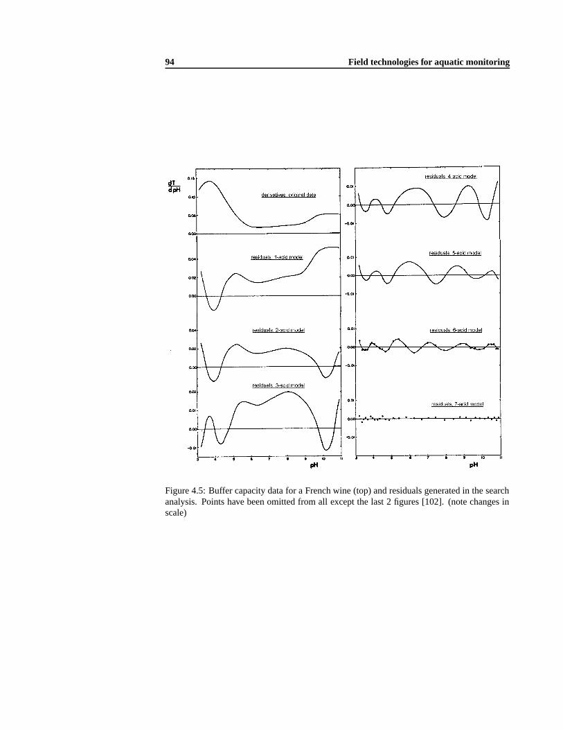
94 Field technologies for aquatic monitoring
Figure 4.5: Buffer capacity data for a French wine (top) and residuals generated in the searchanalysis. Points have been omitted from all except the last 2 figures [102]. (note changes inscale)

4.4 Titrimetric sensors and applications 95
moval [91]. Biological nitrogen removal includes hydrolysis and degradation of N-containingorganic compounds, nitrification (biological oxidation of NH+
4 to NO�3 ) and denitrification
(NO�3 reduction to N2). Monitoring the reaction rates of these processes is possible with regu-
lar sampling and laboratory analyses. These measurements are expensive, time consuming andoften not usable for on-line control. In activated sludge systems with highly varying processconditions, such as for instance in sequencing batch reactors or alternating activated sludgeplants, on-line estimation of in-situ nitrification and denitrification rates is possible based onthe data provided by on-line NH+4 and NO�3 analyzers [171] (see also section 4.2). For contin-uous flow activated sludge systems, however, batch experiments are needed to obtain similarinformation on the sludge characteristics because continuous input of influent results in datawith very little dynamics so that no clear interpretation can be made [316]. Therefore, the con-cept of adaptive in-sensor-experiments was developed [315,316]. An in-sensor-experiment istypically performed in a down-scaled bioreactor in which the full-scale process is simulated inhardware, and to which specific manipulations such as substrate additions are performed to ob-serve the dynamic response of the biological process. The experimental conditions for whichan in-sensor-experiment provides the most interesting data may vary as the conditions in thefull-scale process change. It is therefore an essential feature of measuring systems operatingaccording to the in-sensor-experiment principle to be capable to automatically adjust the exper-imental conditions in the sensor. This automated adaptation leads to the concept of the adaptivesensor [316]. Some applications based on the principle of (adaptive) in-sensor-experiments arepresented in the next paragraphs.
In similar sensors (BRAM: Biological Residual Ammonium Measuring system; ANITA:Ammonium NITrification Analyzer) the stoichiometric conversion of NH+
4 into NO�3 produc-
ing H+ is used to measure the residual ammonium concentration and the activity of the nitrifiersin an activated sludge sample [88, 92, 180]. The biosensor is made of a reactor vessel and a pHtitration unit. Activated sludge, taken from a WWTP, is transferred to the vessel. Acid or baseis added to adjust the pH to a chosen set-point. After this phase, cumulative alkali addition isrecorded to maintain the set-point pH. The slope of the linear part of the alkali addition profileis closely related to the actual NH+4 -N removal velocity, unless aerobic acidifying microbialpopulations other than nitrifiers are present [181]. The total amount of base needed is relatedto the NH+4 present. Recovery experiments in which a range of concentrations from 0.5 to 4mg NH+
4 -N l�1 was added to mixed liquors free of ammonium resulted in errors from 1 to 8% [181]. Further refinement of the sensor consisted in a pulse dosing of approximately 1.3 mgNH+
4 -N l�1 at the beginning of each measurement cycle. This enabled to measure the nitrifica-tion rate of an activated sludge sample even when almost no NH+
4 -N was initially present in thesludge sample [88]. Theoretically, the calculation of the results could be simplified by choosingthe pH set-point exactly the same as the equilibrium pH. Eventually the equilibrium pH couldbe changed by adjusting the % CO2 in the gas phase of the aeration air, but this would makethe titration system more complicated and more expensive to operate [88]. The influence ofchanges in operational factors such as pH, temperature and bicarbonate alkalinity on the NH+
4measurements has been examined [180]. An increase in the amount of bicarbonate buffer inthe mixed liquor had a considerable effect on the accuracy of the results, even for a variation of1 meq l�1, because the increase in the amount of bicarbonate buffer decreased the sensitivityof the pH sensor and therefore the accuracy of the titration. A decrease in total ammoniumwith increasing bicarbonate concentration was observed [180]. This error can be overcome by

96 Field technologies for aquatic monitoring
independent determinations of the alkalinity, allowing variable quantities of strong acid in thereaction vessel to be added. In this way, the titration system is operated at constant alkalinity[180]. With the same sensor, it was possible to estimate the volumetric nitrification capacityof the mixed liquor and the Monod half-saturation coefficient for theNitrosomonasbacteriain the sludge. These kinetic parameters are determined with an existing parameter estimationprocedure on the basis of information provided by a titration in-sensor-experiment using a ni-trifying activated sludge sample [92]. The same method was also used to quantify the effectof low concentrations of a toxic compound on the kinetic parameters of ammonium oxidizingbacteria [90]. The experimental results showed that two sludge samples reacted completelydifferent in the presence of a certain concentration of the same toxic compound.
DECADOS (DEnitrification CArbon source DOsage System) is a biosensor for denitrifi-cation control in activated sludge WWTP [40, 91, 181, 312]. It is based on two simple androbust probes (pH and ORP). The sensor provides relevant information concerning the kineticsand stoichiometry of the denitrification process and, under some conditions of the in-sensor-experiment, the concentration of nitrate [91]. The sensor is equipped with 3 pumps: acid, baseand carbon source dosage pumps. A sample of activated sludge mixed liquor is pumped intoa 1 litre vessel and the titration with the carbon source is started. The titration end-point isdetected by monitoring the Oxidation Reduction Potential (ORP) of the mixed liquor, based ona particular pattern when all nitrate is consumed (nitrate knee) [181]. The proton consumptionis measured via the acid/base addition rate of a pH controller that keeps the pH at a set-point. ApH controller is used, rather than a mere pH measurement, because this excludes the influenceof buffering components and simplifies the theoretical background of the sensor [40]. Fromthe volume of carbon source solution added, the nitrate concentration and denitrification ratecan be calculated. In case a readily biodegradable substrate is used as titrant, the volume ofthat carbon source of unknown composition that is needed per volume unit mixed liquor tocompletely remove the nitrate present can also be measured with the DECADOS.
Another denitrification based sensor is the DENICON (DENItrification CONtroller). It isbased on a titration unit similar to the one described for the BRAM system [181]. DECADOSis a closed system, while DENICON is an open system with N2 and CO2 sparging. The infor-mation provided by the DENICON is similar to that of DECADOS [181]. In the DENICON,anoxic conditions are created with a mixture of N2 and CO2 bubbled through the measuringvessel. Nitrate and sodium acetate are added to the mixed liquor in excess to the assumed max-imum required nitrate concentration in the ratio of 1 : 5 (N : CH3COO�). A modified versionof the DENICON was used to measure VFA concentration in digested anaerobic liquors asreadily biodegradable COD. A sample of the digested effluent is mixed to denitrifying micro-organisms in the presence of excess nitrate. The concentration of readily biodegradable CODis then derived from the consumption of nitrates, as measured by titration [242]. This sensormight allow for a better process control of the majority of the anaerobic reactors, which are fedon variable feed both as flow and concentration [242].

Chapter 5
Software developments
5.1 pH titration algorithms
Commercial automatic titrators have built-in algorithms for the control of a titration exper-iment. A complete titrator set-up consists of a dosing unit for the titrant, a pH meter andtitration algorithms. These titration algorithms perform tasks like
� pH measurement and pH stabilization detection,� calculation of the amount of titrant to be dosed during the titration course, and� end-point detection.
The details of titration algorithms are kept secret by the titrator developers, because of theircommercial value. Two similar titrator set-ups, with and without built-in titration algorithmshave a purchase price difference of minimume3000. In the framework of this research, only alimited number of functionalities out of the wide range of possibilities that commercial titrationalgorithms offer, are needed. Therefore the objective of this section is to develop a titrationalgorithm, capable of performing just the titration task as is needed for this work.1
The commercial titrator used throughout this work is the Metrohm Titrino 716 [168], how-ever other commercial titrators (Orion 960 Titrator Plus System and Mettler DL70 Titrator)were also evaluated and found similar concerning the capabilities of the titration algorithms.
In the following sections, first the built-in algorithms of the Titrino 716 will be presentedand discussed; then three sections follow describing alternative titration algorithms developedin the framework of this research. These alternatives will be classified into a data-based ap-proach, a model-based approach and a combined data- and model-based approach.
1It should be mentioned that the research results described in this thesis are based on titrations performed with acommercial titrator with built-in titration algorithms. The alternative titration algorithm developed in this chapter hasbeen implemented in a prototype sensor, however, only at the end of this Ph.D. study.

98 Software developments
5.1.1 The Dynamic Equivalence-point Titration (DET) algorithm
The Metrohm Titrino 716 is an advanced titrator system for laboratory use. The titration modedetermines the manner in which the titration is performed. The following titration modes canbe selected on the Titrino 716 [168]:DET : Dynamic Equivalence-point Titration. With this type of titration, the titrant is added
in differently sized volume increments: In the flat part of the curve, the increments arelarge, whereas in the steep part small increments are added. This mode is suitable formost titrations. However, the algorithm for reagent dispensing functions perfectly onlyif the curve does not deviate too much from an S-shaped profile.
MET : Monotonic Equivalence-point Titration. With this type of titration, the titrant is addedin volume increments whose size does not change throughout the entire titration. Thismode is suitable for slow titration reactions (e.g. diazotisations, coupling reactions) orfor titrations with asymmetrical curves.
SET : Set Endpoint Titration. This mode is suitable for very fast routine determinations, anddispenses continuously until the stop criterion is reached.
Throughout this work, titration curves were taken with the DET algorithm. The choice forthis algorithm was straightforward, because of the following reasons:
� The DET algorithm tends to ensure a constant measurement point density and ensures aconstant weight of all pH regions for further data processing.
� The SET algorithm does not take into account electrode kinetics and equilibration times;therefore it is not useful in the framework of this research.
� The MET algorithm with a medium volume step works too slow in the pH regions wherethe buffer capacity is high (e.g. pH< 4 or pH> 10) and works too fast in the low buffercapacity regions (e.g. pH 7), with as consequence a lack of data points in the low buffercapacity regions.
The technical details of the DET algorithm are not available for the end-user, except thatthe algorithm is sensitive to deviations from the S-shape: : : However, the available titrationparameters that can be tuned by the user illustrate the basic functioning of the algorithm. Themost important titration parameters of the DET algorithm are:
� Measurement point density (0�9): 0 is the highest density. For a value of 4 (default),experimental results show a point density that typically varies between 2 and 20 mea-surement points per pH unit. An example of a titration, with the lowest and highestpossible measurement point density in the DET algorithm, is shown in Figure 5.1.
� Minimum increment: Minimum volume to be dispensed between 2 successive titrationpoints. The DET algorithm always dispenses 3 times this volume at the beginning of thetitration.
� Titration rate: Dosing rate for increments (default = maximum).� Signal drift: Drift criterion for measured value acquisition (default 1mV min�1).� Equilibration time: Waiting time for measured pH value acquisition. It is used in com-
bination with the signal drift. The algorithm proceeds to the next point when the signaldrift criterion or the equilibration time criterion is reached (default = 60s).
� Stop pH: End pH value. The algorithm stops when the stop pH or the stop volume isreached.

5.1 pH titration algorithms 99
2
3
4
5
6
7
8
9
10
0 1 2 3 4 5 6 7 8 9 10 11 12
pH
ml NaOH 0.1 N added
5 points
9 points
(a)
2
3
4
5
6
7
8
9
10
0 1 2 3 4 5 6 7 8 9 10 11 12
pHml NaOH 0.1 N added
7 points
16 points
(b)
Figure 5.1: Lowest (a) and highest (b) measurement point density with the DET [168] algo-rithm for a titration of 10ml oxalic acid 0.1N in 150ml water with NaOH 0.1N as titrant
� Stop volume: Maximum allowed titrant volume for a complete titration.
Besides the titration parameters, there are also parameters related to equivalence-point eval-uation. In the framework of this research, equivalence-point determination was only used fortitrations of e.g. oxalic acid, for the calculation of the exact normality of the NaOH titrant.
Despite the fact that the DET algorithm gave satisfactory results throughout this work, anumber of remarks about this algorithm are given below. First, the measurement point densitycontrols only partially what we want to realize, i.e. a constant∆pH step, or in other wordsa constant number of measurement points per pH unit. This equidistant measurement pointdensity is advantageous for the further data processing, more particularly for the calculationof the buffer capacity from the titration profile, because this calculation is based on a movingwindow parabolic regression on the raw titration data. The DET algorithm gives a high orlow measurement point density in regions with respectively high or low buffer capacities. Thisoften results in too low measurement point densities in these parts of the titration curve thatare very important for the later data processing part, e.g the region around pH 7. This isclearly illustrated in Figure 5.1. Plot (a) with the lowest measurement point density realizesa density of 9 points between pH 3 and 4 (a high buffer capacity region), and only 5 pointsbetween pH 6 and 7 (a low buffer capacity region). Plot (b) with the highest measurementpoint density, realizes for the same pH regions 16 and 7 points respectively. The minimumrealized volume increment between pH 6 and pH 7 was 60µl, which is still above the minimumincrement volume, that was set to 10µl in this example. Based on this, one can concludethat the measurement point density parameter mainly controls the number of points in the highbuffer capacity region (often the less interesting part of the curve), but does not highly influencethe number of points in the low buffer capacity region. Further it is not possible with the DETalgorithm to obtain a titration curve with a constant, and user-adjustable∆pH step.
Second, the successively realized∆pH steps during the course of a titration show slow andfast changes which cannot be controlled by the user. This is illustrated in Figure 5.2. Plot(a) shows a titration curve of oxalic acid, titrated with a measurement point density of 4, the

100 Software developments
default value. Plot (b) are the calculated successive∆pH values from plot (a). The titrationcurve was taken with a well maintained pH electrode and under the best possible laboratoryconditions. The first 3 steps are steps of 10µl, the minimum dispensable volume, which is oneof the DET titration parameters presented before. Based on these 3 steps, a first relevant∆pHof 0.03 is realized. Then the titration algorithm slowly increases the∆pH to 0.1, and keeps thispH step for a number of points. After this, the titration algorithm slowly increases its pH stepsize to about 0.2 units, until the point where the equivalence-point is almost reached. Aroundthe equivalence-point, the∆pH is not stable and varies between 0.2 and 0.45. In that region,the titrator controller also reaches two times its saturation value for the minimal incrementvolume (10µl, indicated with an arrow). From this∆pH analysis, it can be concluded thatthe titration algorithm uses other rules for the titration advancement than a constant∆pH. Theprimary function of the DET algorithm is to detect and quantify end-points, and relatedKa
values (inflection points) of simple buffer systems.From Figure 5.2(b) it can be suggested that the DET titration algorithm initially proceeds
with a constant, and positive second derivative, followed by a region with second derivativeequal to 0 (in particular the region that starts after the inflection point of the oxalic acid buffer,indicated with a filled symbol on the plot). The∆pH’s in the final part of the titration curveare more irregular, and more difficult to interpret in function of the titration algorithm. Furtherthe ‘Instructions guide’ [168] mentions also something about the second derivative approach,but without any details: “The evaluation of EP’s is based on the zero crossing of the secondderivative with a Metrohm correction for the distortion of the curve from superimposed jumps”.Both the end-point andpKa value are inflection points on the titration curve, which points tothe necessity of a second derivative analysis of the titration data. From this, one can concludethat the DET algorithm is based on a second derivative analysis, in function of inflection pointdetermination, but that for the purpose of this work, a first derivative approach (constant∆pH)would be sufficient. Further, a second derivative analysis is very sensitive to data taken underunideal circumstances (e.g. noisy data). This will be illustrated in the next point.
Third, some remarks can be made when the DET titration algorithm is used in situationswhere the recorded titration curve differs from an ideal smooth, S-shaped titration curve. Sit-uations where the titration curve deviates from the ideal case are manifold:
� pH electrode related: fouled diaphragm, electrolyte level too low, electrode too slow,: : :� pH amplifier related: electrical interferences, noisy amplification, ground loops,: : :� Titrant related: contamination with e.g. CO2 in NaOH titrant.� Dosing unit related: air bubbles in the tubings,: : :� Sample related: Slow chemical reactions, exchanges with atmosphere,: : :
Two such examples are given in Figure 5.3. In this particular case, some problems existedwith the pH electrode, where the electrolyte level was no longer high enough to ensure thenecessary positive outflow of electrolyte to the solution. At first sight the electrode seemed towork correctly, so the problem related to the low electrolyte level was not noticed immediately.The plots (a)+(c) and corresponding plots for∆pH (b)+(d) illustrate 2 noisy titration curvesof oxalic acid. The DET algorithm was set to find 1 equivalence-point, and then stop thetitration (as only oxalic acid was present, it was considered that the algorithm would find only1 equivalence-point, similar as in Figure 5.2). However in both cases the algorithm stopped tooearly, far before the real equivalence-point. Plots (c) and (d) shows a situation where the∆pH

5.1 pH titration algorithms 101
2
3
4
5
6
7
8
9
10
0 1 2 3 4 5 6 7 8 9 10 11 12
pH
ml NaOH 0.1 N added
(a)
0
0.1
0.2
0.3
0.4
0.5
0 5 10 15 20 25 30 35 40 45 50 55
∆pH
Measurement point
(b)
Figure 5.2: Titration curve (a) and corresponding steps in pH for successive titration points (b)for a titration of 10ml oxalic acid 0.1N in 150ml water with NaOH 0.1N as titrant (the arrowsindicate that the minimum allowable volume was dosed; the filled symbol on the titration curvecorresponds with thepKa value of oxalic acid as determined by the DET algorithm)
is even negative. From a theoretical point of view this is not possible, because consecutivealkali additions should result in a pH increase. This phenomenon is e.g. also noticed when anair bubble from the titrant tubing is brought into the titration vessel, or when the pH electrodeis not stable yet when the pH measurement is already performed. In such cases, the DETalgorithm typically will give a too high titrant step volume for the next point in the titrationcurve. Data as shown in Figure 5.3 also create difficulties in further data processing, e.g. forthe calculation of the buffer capacity, which is based on the first derivative of the titration data.A typical problem in the calculation of derivatives is the amplification of noise present in theoriginal raw data. From these findings one can conclude that the DET algorithm is not a veryrobust algorithm for our purpose, and it can possibly fail in situations deviating from the idealsituation. This is justified by the fact that the algorithm was developed for a titrator that is usedin a laboratory environment, under perfect measurement conditions, and for equivalence-pointdetection only.
It was mentioned before that the majority of the titration curves in this research were takenin the lab with the Titrino 716 titrator and with the DET algorithm, because this titration systemwas readily available in the lab and generally gave good results. Titrations where the DETalgorithm failed were repeated again until an acceptable titration curve was obtained. Howthe DET algorithm performs on more complex samples is illustrated in Figure 5.4, which is atitration curve of a destructed and diluted manure sample, containing at least carbonate, ortho-phosphate and ammonium (see chapter 8). The DET algorithm realizes∆pH steps that varybetween 0.02 and 0.4 pH units.
The aim of this work includes the development of a field applicable on-line measuring sys-tem, and therefore alternative, tailor-made algorithms are worked out in the next three sections.Three different approaches are taken: First, an approach is proposed where the titration algo-rithm only relies on the titration points (data) which are already collected (this corresponds

102 Software developments
2
3
4
5
6
0 1 2 3 4 5 6 7 8 9 10
pH
ml NaOH 0.1 N added
(a)
2
3
4
5
0 1 2 3 4 5 6 7 8 9
pH
ml NaOH 0.1 N added
(c)
0
0.1
0.2
0.3
0 5 10 15 20 25 30 35
∆pH
Measurement point
(b)
0
0.1
0.2
0.3
0 5 10 15 20 25 30
∆pH
Measurement point
(d)
Figure 5.3: Titration curves (a)+(c) and corresponding steps in pH for successive titrationpoints (b)+(d) for a titration of 10ml oxalic acid 0.1N in 150ml water with NaOH 0.1N astitrant (an arrow indicates that even negative∆pH’s can be found in real curves)
2
3
4
5
6
7
8
9
10
11
0 0.2 0.4 0.6 0.8 1 1.2
pH
meq NaOH added
(a)
0
0.1
0.2
0.3
0.4
0 5 10 15 20 25 30 35 40 45 50 55 60
∆pH
Measurement point
(b)
Figure 5.4: Titration curve (a) and corresponding steps in pH for successive titration points (b)for a titration of a destructed and diluted animal manure with NaOH as titrant

5.1 pH titration algorithms 103
with the DET algorithm, so no a priori knowledge about the sample is used). This is the data-based approach. In the second approach, a priori knowledge about the buffer systems thatare to be expected is introduced in the titration algorithm. This approach is the model-basedapproach. The third approach is a combined data- and model-based approach. The two mostimportant criteria that were used for the algorithm development are:
� a user-defined set-point for∆pH, and� a robust algorithm that will not give irregular jumps in∆pH when the titration is not
performed under ideal conditions.
5.1.2 Data-based titration algorithm
In its simplest form the data-based approach is an algorithm that can predict the consecutivetitrant volume steps to be dispensed, in order to change the pH with the set-point∆pH. It isbased on an extrapolation of the titration curve based on the titration points realized thus far.Two approaches are presented in this section: First, a moving window regression approach,and second, a proportional-integral (PI) controller approach.
In the first approach, practically, a moving window containing thex last titration pointsis used to predict the next point. An initial titration sequence to initiate such extrapolationalgorithm is a necessity (e.g. in a similar approach the DET algorithm uses the first 3 titrationpoints that are a result of dispensing 3 times the minimal incremental volume). Two furtherquestions need to be answered in this framework:
� What is the number of titration points that will be used in the moving window?� Which mathematical algorithm will be used for the prediction of the next point?
Experimental analysis of typical titration curves has shown that in a situation in which eachtitration step is around 0:2�0:5 pH units, the ideal number of points in the moving window ismore than 2, but less than 5. Thus 3 or 4 points make a good compromise between robustnessor smoothness of the prediction (more points = more robust) and the actual dynamical responseof the pH signal (less points = better pH dynamics). In the following examples 3 points will beused for the window width.
If 3 points are used for the window width, the possible choices for the mathematical modelthat can be used for the prediction of the next point are rather limited. A linear or parabolicregression model are reasonable choices that will be further discussed. Two examples withboth a linear and parabolic regression model are given in Figure 5.5. Under ideal measurementconditions, i.e. a smooth S-shaped titration curve, the parabolic regression is superior to thelinear regression, especially in the low and high pH regions. This is illustrated in Figure 5.5(a),and can be interpreted as follows: Assume that one has titrated until point 3, and we wantto predict the next titrant volume step∆V for a chosen set-point∆pH = 0:2. The predictedvolume steps with respectively the linear and the parabolic regression are∆V1 and∆V2. It canbe seen that the linear regression line predicts a too high volume step∆V1 for the desired set-point ∆pH, whereas the parabolic regression line predicts an almost perfect volume step∆V2.In the high pH range (not shown on the figure), the linear regression predicts too small volumesteps, whereas the parabolic regression predicts correct volume steps. In the pH range 5�8,both regression types give similar results. Thus, in an ideal case, the parabolic regression is

104 Software developments
3
3.5
4
4.5
5
5.5
6 6.5 7 7.5 8
pH
ml NaOH 0.1 N added
12
3
(a)
∆V1
∆V2
set-point ∆pH = 0.2
linear regressionparabolic regression
3.5
4
4.5
5
6 6.5 7 7.5 8 8.5 9 9.5 10
pH
ml NaOH 0.1 N added
12 3
(b)
∆V1
set-point ∆pH = 0.2
linear regressionparabolic regression
Figure 5.5: Illustration of linear and parabolic regression used for the data-based titration algo-rithm. Plot (a): titration curve taken under ideal circumstances. Plot (b): non-ideal situation.Points 1, 2 and 3 are used in the regressions
the best choice. The situation is, however, completely different when titrations are performedunder non-ideal circumstances (see also section 5.1.1). Such example is given in Figure 5.5(b).Assume again that one has titrated until point 3, and we want to predict the next titrant volumestep∆V for a chosen set-point∆pH = 0:2. For the illustrated example, the titrant volumestep needed to increase the pH with the set-point∆pH cannot be predicted with the paraboliccurve. This is explained by the noisy data in that part of the titration curve, and consequently acalculated parabolic regression curve that completely fails to represent the shape of the titrationprofile. On the other hand, the linear regression over-predicts with a factor 2 the volume stepto be dispensed. Therefore, algorithms based on extrapolation of titration points fail in casethe titration curve differs from ideality. In other words these algorithms are not very robust,a disadvantage for e.g. field-use of such algorithm. This finding corresponds with what wasillustrated in section 5.1.1, because the DET algorithm is also a data-based algorithm.
In the second approach, a PI-controller is evaluated for the purpose of constant∆pH titra-tion. The PI-model in discrete notation is shown in equation (5.1).
∆V(k+1) = ∆V(k)+KC ε(k)+KC
τI
k
∑i=1
ε(i) (5.1)
k : titration point number∆V(k) : volume pulse to be dispensed at titration pointkKC : proportional control constantτI : integral control constantε : ∆pHrealized�∆pHset-point
The performance of this PI-controller was evaluated with simulation examples, and optimumvalues forKC andτI were searched. However, no optimum values were found, and no decentcontrol was realized. The non-linear behaviour of the pH in function of the volume steps of

5.1 pH titration algorithms 105
titrant added is pointed to be the reason why this type of control was not working. Thus itwas concluded that PI-control is not suited for the purpose of constant∆pH titration. This is incorrespondence with literature findings, that pH control by conventional means is very difficultbecause of the highly non-linear response of the pH value to the addition of acid or base [188].A more advanced and adaptive pH controller was successfully implemented for a pH wastew-ater neutralisation process [135]. The controller is based on a neural network, and both thenetwork structure and the related parameters (weights) are updated on-line. Another success-ful pH controller, based on fuzzy logic was found useful for pH control of laboratory reactors,waste streams,: : : [188]. The pH controller is based on fuzzy logic because it permits theinclusion of subjective knowledge, often based on experience and not on a theoretical model.The knowledge supplied to the control system includes e.g. prior experimental results. How-ever, for the purpose of titration algorithm development, there is theoretical knowledge aboutthe system available. Therefore it should be worthwhile to include this a priori knowledge inthe algorithm. Such type of titration algorithm is the topic of the next section.
5.1.3 Model-based titration algorithm
Up to this point, no a priori knowledge about the sample was used in the titration algorithm.However, in most cases, quite a lot of information about the sample to be titrated is available.Useful information can be a list of buffer systems that are to be expected, as well as a first,rough, estimation of their concentrations. As all titrations in this work are in aqueous solution,we know that the water buffer system will be the most significant buffer when the pH< 4 orpH> 10.
Therefore, in this approach, the prediction of the volume step that has to be dispensed inorder to have a change in pH equal to the desired∆pH, will be based on a mathematical model(called titration model) of a hypothetical titration curve calculated with the a priori knowledgethat is available about the sample (expected concentrations andpKa values of buffers). A majorconcern of this approach is the effect incomplete a priori information has on the titration curvethat is being recorded. For instance one may lack information concerning the buffers that arepresent, or the expected concentrations may be deviating too much from the real concentra-tions.
A specific computer program (dyntit) was developed to simulate a model-based titrationbased on 2 input files, containing a ‘real’ titration curve and a ‘titration model’ curve respec-tively. The first input file contains the data of a titration experiment conducted with the labo-ratory titrator and the DET algorithm. The second input file contains simulated titration data,based on the assumed composition of the sample to be titrated. With this software, it waspossible to investigate the effect of the ‘titration model’ on a recorded titration curve, but with-out having to conduct the model-based titration experimentally. The principle implemented indyntit is illustrated in Figure 5.6. A two-step sequence is needed for the calculation of eachtitration point withdyntit. Assume that one has titrated until pH 4, and we want to simulatethe next titrant volume step for a chosen set-point∆pH= 0:8. 2 First, the actual pH and theset-point pH (which is 4.8) are needed to calculate with the titration model curve the volume∆V to be dispensed (points (1) and (2) on Figure 5.6(a)). Second, this volume step is used to
2A more realistic set-point would be∆pH= 0:1�0:2, however, for illustration purposes a higher set-point is taken.

106 Software developments
3
3.5
4
4.5
5
5.5
6
0 1 2 3 4 5 6 7
pH
ml NaOH 0.1 N added
(a)
set-point ∆pH = 0.8
∆V(2)
(1)
3
3.5
4
4.5
5
5.5
6
0 1 2 3 4 5 6 7
pH
ml NaOH 0.1 N added
(b)
realized ∆pH = 1.27
∆V(3)
(4)
Figure 5.6: Illustration of model-based titration as implemented in the softwaredyntit. Plot(a): ‘titration model’ curve. Plot (b): ‘real’ titration curve. The numbers (1)�(4) indicate theconsecutive steps in the algorithm
calculate with the real titration curve the realized∆pH (points (3) and (4) on Figure 5.6(b)).As illustrated, linear interpolation between the real experimental data points is used for thispurpose. In this example the realized∆pH = 1:27, thus the model-based titration algorithmhas overpredicted the required titrant volume step at pH 4. The new actual pH value is now5.27, and the two-step sequence can be repeated to calculate the next point of the hypotheticalrecorded titration curve. Summarized,dyntit generates a hypothetical model-based recordedtitration curve, based on a titration model and a real experimental titration curve. Two exam-ples below will illustrate the model-based titration approach usingdyntit.
A first example is a study based on a simulated titration curve that was introduced in sec-tion 2.2.5 on page 21. This titration curve (here the ‘reality model’ because it represents the‘real’ titration curve indyntit) represents an aquatic sample containing some carbonate, ortho-phosphate, ammonium and an organic acid buffer. A simulation study was set up to investigatethe effect of a wrongly defined ‘titration model’ in terms of the model versus the real bufferconcentrations. For the simulation study, two titration models were tested: Model 1 incor-porates all buffers that are present in the ‘reality model’, but with concentrations equal to 50% of the real concentrations (except the water buffer concentration, which is always 55.5M).Model 2 is a similar model, but with concentrations equal to 200 % of the real concentrations.With these 2 titration models, and the ‘reality model’, the model-based titration algorithm wastested. The pH interval was chosen between pH 3 and pH 11, and the set-point∆pH was cho-sen at 0.1 pH units. Thus, for each simulated titration step, model 1 or model 2 were usedto predict the volume needed to increase the pH with 0.1 units, and the ‘reality model’ wasused to find the realized∆pH. The obtained simulation results are shown in Figure 5.7. Atthe beginning and at the end of the titration experiment, the model-based titration algorithm isable to maintain the set-point∆pH of 0.1 units. This is due to the water buffer which is themain buffer in the pH regions outside the pH interval 4�10, and which is correctly defined inthe titration model (55.5M). Inside the pH interval 4�10, it can be seen that if the titration
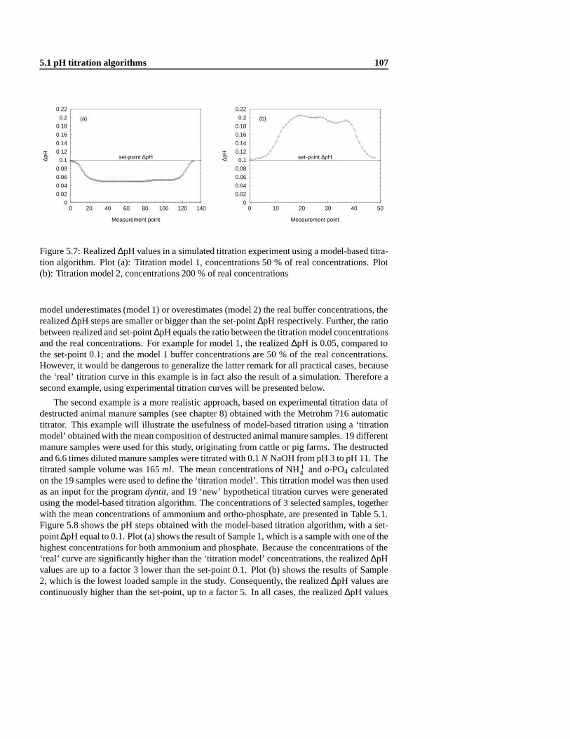
5.1 pH titration algorithms 107
0
0.02
0.04
0.06
0.08
0.1
0.12
0.14
0.16
0.18
0.2
0.22
0 20 40 60 80 100 120 140
∆pH
Measurement point
(a)
set-point ∆pH
0
0.02
0.04
0.06
0.08
0.1
0.12
0.14
0.16
0.18
0.2
0.22
0 10 20 30 40 50
∆pH
Measurement point
(b)
set-point ∆pH
Figure 5.7: Realized∆pH values in a simulated titration experiment using a model-based titra-tion algorithm. Plot (a): Titration model 1, concentrations 50 % of real concentrations. Plot(b): Titration model 2, concentrations 200 % of real concentrations
model underestimates (model 1) or overestimates (model 2) the real buffer concentrations, therealized∆pH steps are smaller or bigger than the set-point∆pH respectively. Further, the ratiobetween realized and set-point∆pH equals the ratio between the titration model concentrationsand the real concentrations. For example for model 1, the realized∆pH is 0.05, compared tothe set-point 0.1; and the model 1 buffer concentrations are 50 % of the real concentrations.However, it would be dangerous to generalize the latter remark for all practical cases, becausethe ‘real’ titration curve in this example is in fact also the result of a simulation. Therefore asecond example, using experimental titration curves will be presented below.
The second example is a more realistic approach, based on experimental titration data ofdestructed animal manure samples (see chapter 8) obtained with the Metrohm 716 automatictitrator. This example will illustrate the usefulness of model-based titration using a ‘titrationmodel’ obtained with the mean composition of destructed animal manure samples. 19 differentmanure samples were used for this study, originating from cattle or pig farms. The destructedand 6.6 times diluted manure samples were titrated with 0.1N NaOH from pH 3 to pH 11. Thetitrated sample volume was 165ml. The mean concentrations of NH+4 ando-PO4 calculatedon the 19 samples were used to define the ‘titration model’. This titration model was then usedas an input for the programdyntit, and 19 ‘new’ hypothetical titration curves were generatedusing the model-based titration algorithm. The concentrations of 3 selected samples, togetherwith the mean concentrations of ammonium and ortho-phosphate, are presented in Table 5.1.Figure 5.8 shows the pH steps obtained with the model-based titration algorithm, with a set-point∆pH equal to 0.1. Plot (a) shows the result of Sample 1, which is a sample with one of thehighest concentrations for both ammonium and phosphate. Because the concentrations of the‘real’ curve are significantly higher than the ‘titration model’ concentrations, the realized∆pHvalues are up to a factor 3 lower than the set-point 0.1. Plot (b) shows the results of Sample2, which is the lowest loaded sample in the study. Consequently, the realized∆pH values arecontinuously higher than the set-point, up to a factor 5. In all cases, the realized∆pH values

108 Software developments
Table 5.1: Concentrations of ammonium and ortho-phosphate of three selected manure sam-ples and the concentrations used in the titration model used for the evaluation of the model-based titration algorithm
Concentrations in destructed Model-basedand diluted manure samples titration results
mgNH+4 -N l�1 mg o-PO4-Pl�1
Sample 1 36.0 9.7 Figure 5.8(a)Sample 2 7.6 0.5 Figure 5.8(b)Sample 3 21.4 9.4 Figure 5.9(d)Titration Model 18.7 5.9
varied between 0.03 and 0.5, which are still acceptable in the framework of buffer capacitymodelling. When these results are compared with the results that were obtained with the DETalgorithm (see e.g. Figure 5.4), one notices that the model-based∆pH results are less noisythan the DET results.
5.1.4 Combined data- and model-based titration algorithm
A data- and a model-based titration algorithm were presented in sections 5.1.2 and 5.1.3 re-spectively. It was already suggested that the data-based algorithm is sensitive to fail whennoise or irregular jumps are encountered in the titration data. The model-based algorithm issuggested to be much more robust on this point, because the titration data that are already ob-tained arenot used for the prediction of the volume to be dispensed for a next titration point.On the other hand, the data-based algorithm is expected to keep the realized∆pH close to theset-point∆pH in different types of samples (low and high loaded samples), compared to themodel-based approach where the realized∆pH is only close to the set-point∆pH when thetitration model does not deviate too much from the ‘real’ titration curve. The question is nowif it is worthwhile to combine the 2 approaches and thus use a combined data- and model-basedtitration algorithm.
An example introduced in section 5.1.3 (Table 5.1, Sample 3) was evaluated for this pur-pose, and the results are shown in Figure 5.9. Plots (a) and (b) show the experimental titrationcurve and the corresponding pH steps as obtained with the automatic titrator in the lab, usingthe DET algorithm. Plot (c) is the application of a linear and parabolic regression method forthe data-driven prediction of the next point of the titration curve with a∆pH set-point of 0.1(see also section 5.1.2). A moving window width of 3 points gave the best results, and is shownon the graph. The parabolic regression method keeps the∆pH very close to the set-point, ex-cept for 2 peaks in the beginning and in the middle of the curve. The linear regression lineoverpredicts the volume to be dispensed in the beginning of the titration, and underpredicts thevolume to be dispensed in the last part of the titration. Similar to Figure 5.8, plot (d) representsthe ∆pH values realized when the model-based titration algorithm is used. Because the real

5.1 pH titration algorithms 109
0
0.02
0.04
0.06
0.08
0.1
0.12
0.14
0.16
0.18
0.2
0 20 40 60 80 100 120
∆pH
Measurement point
(a)
set-point ∆pH
0
0.1
0.2
0.3
0.4
0.5
0 10 20 30 40
∆pH
Measurement point
(b)
set-point ∆pH
Figure 5.8: Realized∆pH values in a simulated titration experiment using a model-based titra-tion algorithm. Plot (a): Based on an experimental titration curve of Sample 1 (high concen-trations). Plot (b): Based on an experimental titration curve of Sample 2 (low concentrations).
buffer concentrations of manure sample 3 are higher than the mean concentrations used in thetitration model, the∆pH values in plot (d) are somewhat lower than the set-point 0.1.
Based on this example, and the results from the previous sections, it can be concluded that:
� Both the data-based and the model-based algorithm give satisfying results.� The parabolic algorithm is superior to the linear one for maintaining the desired∆pH.� The model-based algorithm is less sensitive to irregular jumps in the realized∆pH.
Therefore a combined data- and model-based algorithm is suggested for a robust and accuratetitration algorithm with constant∆pH steps and with a user-defined set-point for∆pH. Theidea is to have a dual algorithm that predicts the volume to be dispensed with both approaches,and a built-in selector that can select from point to point which of the two calculated volumeswill be dispensed. A flowchart of such dual algorithm is presented at the left side of Figure5.10. The algorithm is proposed for field-use, thus it starts with some diagnostics test to verifyif the titration system is ‘ready for use’. These diagnostics can include a liquid level checkin the titration vessel, an electrode check, etc. The selector algorithm needs to be chosen infunction of the particular application. The selector can either strictly select to dispense thevolume calculated with the model-based or with the data-based approach; or it can select aweighted average of the calculated volumes obtained with both approaches. A high weight forthe model-based approach can be chosen if robustness or fail-safety are important, or a highweight for the data-based approach can be chosen if it is uncertain that the titration model isrepresentative for the titrated sample. A more complicated selector would, for instance, includea detection of a possible irregular jump for a data-based volume step, thus resulting in a lowerweight factor for the data-based approach.
A possible alternative for the selector algorithm is a sequential algorithm, with a model-based volume step, supplemented with a data-driven factor to correct the model-based volumefor previously realized∆pH’s. Such correction factor approach is illustrated at the right side ofFigure 5.10. An example is worked out in the next paragraph.
110 Software developments
2
3
4
5
6
7
8
9
10
11
0 0.2 0.4 0.6 0.8 1 1.2
pH
meq NaOH added
(a)
0
0.05
0.1
0.15
0.2
0 5 10 15 20 25 30 35 40 45 50 55 60
∆pH
Measurement point
(c)
set-point ∆pH
linear regressionparabolic regression
0
0.05
0.1
0.15
0.2
0.25
0.3
0.35
0.4
0 5 10 15 20 25 30 35 40 45 50 55 60
∆pH
Measurement point
(b)
0
0.05
0.1
0.15
0.2
0 10 20 30 40 50 60 70 80 90 100 110
∆pH
Measurement point
(d)
set-point ∆pH
Figure 5.9: Experimental titration curve (a) and corresponding steps in pH for successive titra-tion points (b) obtained with an automatic titrator using the DET algorithm. Realized∆pHvalues in a simulated titration experiment using a data-based (c) and model-based (d) titrationalgorithm based on the experimental titration curve

5.1 pH titration algorithms 111
Dispense volume
Measure pH
Run diagnostics
Run selector algorithm
Stabilizationcriterion fulfilled ?
Stop criterionfulfilled ?
End of titrationYes
Calculate volume tobe dispensed with thedata-based approach
Calculate volume tobe dispensed with the
model-based approach
Yes
No
No
Dispense volume
Measure pH
Run diagnostics
Stabilizationcriterion fulfilled ?
Stop criterionfulfilled ?
End of titrationYes
Calculate data-driven correction factor
Calculate volume tobe dispensed with the
model-based approach
Yes
No
No
Figure 5.10: Flowcharts of a combined (left side) and sequential (right side) model- and data-based titration algorithm for constant∆pH titration
A discrete first-order correction factorζ was applied to the model-based calculated volumesin order to keep the realized∆pH’s closer to the set-point∆pH.
ζ(k+1) = ζ(k)�λ ε(k) andζ(0) = 1 (5.2)
∆V(k) = ∆V(k)model� ζ(k) (5.3)
k : titration point numberζ : correction factorλ : first order constantε : ∆pHrealized�∆pHset-point
∆V(k) : volume pulse to be dispensed at titration pointk∆V(k)model : volume to be dispensed as calculated with the titration model
In equation (5.3), it can be seen that the volume pulse to be dispensed depends on a model-driven term∆V(k)model and a data-driven termζ(k). Equations (5.2) and (5.3) were imple-mented in the programdyntit (introduced in section 5.1.3) to simulate a model-based titration.The example that is presented in section 5.1.3 (Table 5.1, Sample 3) was evaluated again, andsome results are shown in Figure 5.11. The effect of the algorithm tuning parameterλ wasevaluated and for this particular example a value ofλ between 2 and 15 gave significantlybetter results compared to the results obtained without the correction factor, presented in Fig-

112 Software developments
0
0.05
0.1
0.15
0.2
0 10 20 30 40 50 60 70 80
∆pH
Measurement point
(a)
set-point ∆pH
0
0.05
0.1
0.15
0.2
0 10 20 30 40 50 60 70 80
∆pH
Measurement point
(b)
set-point ∆pH
Figure 5.11: Realized∆pH values in a simulated titration experiment using a model-basedtitration algorithm with a first-order correction factorζ. Plot (a)λ = 4. Plot (b)λ = 10
ure 5.9(d). For higherλ values the algorithm became unstable due to an overcompensatingeffect of the data-driven correction factorζ, resulting in a heavily oscillating∆pH around itsset-point.
The 19 different manure samples that were used to define the titration model (section 5.1.3),were evaluated for the effect ofλ and it was found thatλ = 4 is a safe value, in terms of stabilityof the algorithm, giving satisfying∆pH steps around the set-point∆pH. The results forλ = 4for 2 selected samples are shown in Figure 5.12. This figure can be compared with Figure 5.8,that presents the same examples, but without the correction factorζ.
The combined data- and model-based algorithm includes at least the following user-definedtitration parameters:
� Set-point∆pH: The desired increment in pH between 2 successive titration points.� Minimum increment, signal drift, equilibration time, stop volume and stop pH. These
parameters are explained in section 5.1.1.� For the model-based approach: A list of buffers, theirpKa(’s) and concentration(s).� For the data-based approach: Moving window width for the regressions.� For the selector: depending on the user-defined selector algorithm.� For the data-driven correction: First order constantλ.
5.1.5 Validation of the combined titration algorithm
The sequential model- and data-based titration algorithm developed in section 5.1.4 was eval-uated for its usefulness under more realistic conditions. A preliminary set-up for field-use wasrealized with a titration vessel, a computer controlled NaOH dosing unit, a high impedancepH amplifier and an industrial PC with the titration algorithm. Thirty destructed and dilutedmanure samples (10 pig, 10 cattle, 10 poultry) were used for the validation experiment. Themathematical titration curve model used in the titration algorithm was based on the mean com-position of respectively pig, cattle and poultry manure (see also chapter 8).

5.2 Tableau-method based simulation software 113
0
0.05
0.1
0.15
0.2
0 10 20 30 40 50 60 70 80
∆pH
Measurement point
(a)
set-point ∆pH
0
0.05
0.1
0.15
0.2
0 10 20 30 40 50 60 70 80
∆pH
Measurement point
(b)
set-point ∆pH
Figure 5.12: Realized∆pH values in a simulated titration experiment using a model-based titra-tion algorithm with a first-order correction factorζ. Plot (a): Sample 1 (high concentrations).Plot (b): Sample 2 (low concentrations).
The titration curve and the corresponding∆pH steps for 1 selected sample are shown inFigure 5.13. The results for the other samples are comparable. Despite the fact that the pHmeasurement was not very stable yet (signal noise of 3mV or 0.05 pH units), the titrationalgorithm succeeded within acceptable deviations to maintain the set-point∆pH of 0.2 duringthe complete titration, and for the 30 different tested samples. Based on these results, it isconcluded that the developed titration algorithm is sufficiently robust for field-use.
5.2 Tableau-method based simulation software
5.2.1 Software objectives
The programbctabis an acronym for “Buffer Capacity simulation using the chemical equilib-rium Tableau method”. A compact and convenient way to represent stoichiometric data of achemical equilibrium problem is in the form of a ‘tableau’ [198]. This tableau representationis treated in section 3.5 on page 55. The tableau method is used to solve chemical equilibriumproblems, including complexation and precipitation reactions. In section 3.5.3 on page 61, it isillustrated that, with some slight modifications of the original tableau concept (e.g. excludingH+ as a component), it is possible to adapt this method for buffer capacity simulation. Exten-sions to also include ionic activity corrections and precipitation reactions in the buffer capacitysimulation are presented respectively in sections 3.5.4 on page 63 and 3.5.5 on page 64.
From literature, it was found that several software programs exist for chemical equilibriumproblems. Two of them were evaluated in more detail for the purpose of buffer capacity mod-elling. The first program is MINTEQA2 [10], which has found wide use in environmentalapplication areas (see section 2.6 on page 37). The second program is MAGIK [20], which isa set of mathematical routines to solve complex chemical equilibria problems. This softwareuses similar matrix concepts as in the tableau method (see section 3.6 on page 67).

114 Software developments
3
4
5
6
7
8
9
10
11
0 2 4 6 8 10 12 14 16 18 20
pH
ml NaOH 0.1 N added
(a)
0
0.05
0.1
0.15
0.2
0.25
0.3
0.35
0.4
0 10 20 30 40
∆pH
Measurement point
(b)
set-point ∆pH
Figure 5.13: Experimental titration curve (a) and corresponding steps in pH for successivetitration points (b) obtained with the combined model- and data-based titration algorithm andwith a preliminary titration set-up for field-use
The program MINTEQA2 [10] is a speciation program. For a particular set of chemi-cal components specified by the user, MINTEQA2 will equilibrate the chemical solution to aspecified pH and/orEh, to the partial pressure of a gas phase and/or to a specified solid phasecomposition. The molality and activity of the free ions and aqueous complexes are calculated.In addition, the percent distribution of each component among the aqueous species is deter-mined. Metal adsorption submodels and the calculation of saturation indices of solid phasesare also included in the package. The program consists of a number of FORTRAN routines, ofwhich the source code is freely available for the user. The interaction with the user is via in-and output files. The problem should be entered in a specific format file, and this file is thenprocessed by the main program. The results enter in an output file. For a beginning user, it wasexperienced that it is difficult to understand and use the program when one is not very familiarwith the chemical background of the included processes. Even for a small chemical problem,one should consider all possible phenomena, even if one is not interested in those phenom-ena. The simulation of a titration experiment and the related calculation of buffer capacities isnot readily implemented. However, it should be possible to add this functionalities with somemodifications in the source code by an experienced user. It was concluded that MINTEQA2 isa very powerful program, with many features, but not well suited for the purpose of simulationof buffer capacity curves in the framework of this work.
The program MAGIK [20] is less extensive in possibilities compared to MINTEQA2.However, it can simulate titration curves for complex chemical equilibrium systems. The pro-gram is written in FORTRAN, and the source code is also available. The chemical equilibriumproblem should be entered by the user in the form of a FORTRAN subroutine. This user-defined subroutine contains the chemical equilibrium equations and the mass balances. Incase of possible precipitation reactions, a set ofif : : : thenstatements should be entered bythe user. The organization of the chemical problem in a set of FORTRAN commands is notwell-structured, compared to the tableau method. As a consequence, it is difficult to overview,

5.2 Tableau-method based simulation software 115
modify, extend or correct a chemical problem that is entered as a FORTRAN subroutine. Themain program is an implementation of what is described in section 3.5.1 on page 55, i.e. theNewton-Raphson method of steepest descents and partial derivative calculations to constructa Jacobian matrix. Buffer capacity calculations are not readily implemented in the software.A major disadvantage of this program is that for each equilibrium problem, the user-definedsource code needs to be modified, and recompiled with a FORTRAN compiler.
Based on the experiences mentioned above, it was concluded that in the framework of thisresearch, the best option was to develop a new program,bctab, to simulate acid-base titrationsand calculate buffer capacity curves. The objectives for this software are:
� A representation of the chemical problem in a tableau, which can easily be modified.� A direct output of buffer capacities in function of a user-defined pH range.� The availability of a facility to recognize pH intervals where precipitation can occur,
based on a user-defined list with possible precipitates and their solubility products.� User interaction with in- and output files only, to keep the program simple, easy-to-use
and hardware platform independent.� A possibility to integrate this software in the softwarebomb, presented in section 5.3.
Similar to the programs discussed above,bctabis based on equilibrium models. Therefore,it is assumed that the chemical system is at equilibrium at each point of the titration. Thisequilibrium assumption is important to remember because natural systems can be kineticallyconstrained.
5.2.2 Software implementation
The programbctabis developed in C++, and can be compiled on different computer platforms.For this research, a C++ compiler (GNU project C++ compiler, v2.7) on a unix workstation(SGI Origin 200) was used for the development ofbctab. The algorithm for matrix inversionwas adopted from the library ‘Numerical Recipes in C’ [229]. A PC version ofbctab(compiledwith DJGPP, DJ’s GNU Programming Platform, free C++ compiler) and a set of illustrativeexamples is also made available for other users.
The methodology ofbctabis based on an implementation of the tableau method, describedin section 3.5.3 on page 61. The criterion for convergence was slightly modified compared tothe criterion found in [251], and earlier presented in equation (3.99):
jYj jCj
< η for all components (j = 1, : : : m) (5.4)
Yj : remaining error in the material balance for componentjCj : total concentration for componentjη : convergence parameterThe buffer capacityβ is calculated from the species concentrations found with the tableaumethod, as illustrated in equation (3.108). It was first investigated and then concluded thatthe relatively simple Euler approach for the calculation of the first derivative was sufficientlyaccurate. The step value∆pH in the Euler algorithm is a user-defined value. Ionic interaction

116 Software developments
effects were implemented as described in section 3.5.4 on page 63. Therefore, an extra user-defined activity coefficientγH+ is included in the software.
5.2.3 Functionalities description
The programbctabhas an elementary user interface and is command-line driven. The neces-sary input data is supplied to the program by a specific format input file, with a fixed name‘intab’. An illustrative example of a valid ‘intab’ file is given below.
# bctab input file version 3.02 # number of components (H+ is NOT a component)9 # number of species1 # number of solubility products to be tested1 # 0 or 1 for log-file function off or on1 # activity coefficient for H+1e-07 # convergence criterion for Newton-Raphson algorithm3 # simulation start pH11 # simulation stop pH.1 # simulation step pH0.05 # internal delta pH for Euler algorithm
H3PO4 Ca(2+) H+ log_K e- CaHPO4(s)0.0019 0.0012
H3PO4 1 0 0 0 0 0Ca(2+) 0 1 0 0 2 1H2PO4- 1 0 -1 -2.2 -1 0HPO4(2-) 1 0 -2 -9.4 -2 1PO4(3-) 1 0 -3 -21.8 -3 0CaH2PO4+ 1 1 -1 -0.8 1 0CaHPO4(aq) 1 1 -2 -6.7 0 0CaPO4- 1 1 -3 -15.3 -1 0OH- 0 0 -1 -14 -1 0
0.002 0.00125 -6.66
The 10 user-defined parameters are explained in the ‘intab’ file, to make editing convenientfor the user. Lines or parts of lines starting with # are considered as comment. The tableauinformation is entered in the ‘intab’ file in a format as illustrated above. Fields can be separatedby spaces or tabs. The first column contains the labels of the species. The next columnscontain the information of the components. More particularly, in each component column,the following information is supplied: a component label, an initial value for the componentconcentration (mol l�1) used in the Newton-Raphson algorithm, the stoichiometric coefficientsand the total concentration (mol l�1). If m components are defined, then the firstm speciesshould be in the same order as the components. The tableau information finishes with a columnfor the stoichiometric coefficients in H+, and the logK values for each species. A followingcolumn with the labele�, contains the charge of each species. This information is neededin equation (3.109), for the calculation of the buffer capacity. The next columns are optionalcolumns, that contain the precipitation conditions to be tested at each pH value. In the example,

5.3 Buffer capacity optimal model builder 117
the last column should read as: Precipitation of CaHPO4(s) will occur if
1 log[Ca2+]+1log[HPO2�4 ]>�6:66 (5.5)
The command
bctab myfile
will read the ‘intab’ file, and will generate 2 or 3 new files, with the following names:myfile.sim : A two-column file with the simulation results. The first column contains the
pH values, and the second column contains the corresponding buffer capacitiesβ(meq l�1 pH�1).
myfile.spc : A multi-column file with the species concentrations and precipitation information.The first column contains the pH values, and for each species, a column with theconcentration (mol l�1) is added. And last, for each precipitate to be tested, acolumn is foreseen for the message ‘precip’, if precipitation is expected at thecorresponding pH.
myfile.log : This file is only generated when the corresponding parameter in the ‘intab’ file isset to 1. This file contains detailed iteration information of the Newton-Raphsonalgorithm and can be consulted in cases where convergence or numerical prob-lems are noticed.
Throughout this work, several illustrative stoichiometric tableaus have been developed, asinput for the programbctab. They are given in Tables 3.1, 3.2, 3.3, 8.11 and 8.13.
5.3 Buffer capacity optimal model builder
5.3.1 Software objectives
The programbombis an acronym for “Buffer capacity optimal model builder”. The three mainobjectives for this software are:
� Calculate buffer capacity curves from titration curves.� Fit mathematical models to experimental buffer capacity curves with a non-linear least
squares optimization routine. The optimized parameters are concentrations and/orpKa
values of selected buffer systems included in the mathematical buffer capacity model.� Stepwisely and automatically construct the optimal buffer capacity model for samples
with a lack of a priori knowledge about the buffers that are expected in the sample.
A literature research on advanced buffer capacity modelling software yielded rather poorresults. Some software implementations and their related applications are described in moredetail in chapters 3 and 4. The majority of available software programs were developed for onespecific application, e.g. the determination of VFA and HCO�
3 in anaerobic digesters (moreexamples in section 4.4.2 on page 89). Such programs are not portable to other applicationareas for other types of buffer systems. One important exception is the software described in[101, 102], which is also discussed in section 4.4.2 on page 89. This computer program (TI-TAN) analyzes titration data for an unknown solution, and is developed for ‘general purpose’

118 Software developments
use. However, no references more recent than 1982 about this program, its applications, orsimilar programs were found.
In two research projects related to this work (AQMON and FASTNAP, described in re-spectively chapters 6 and 8), the final goal is to develop an on-line, robust and field-usablebuffer capacity based sensor. The central part of this sensor is the data processing, which is thesoftwarebomb. Both projects are driven by commercial final goals, and need specific require-ment or criteria for the developed software, such as stability, fail-safety, reusability, robustness,: : : Therefore it was chosen throughout the software development to use only techniques andmethods that have proven to be stable and robust.
5.3.2 Buffer capacity calculation
The buffer capacityβ as a function of pH may be obtained by plotting the inverse of the slopeof the titration curve versus pH (see section 2.2.6 on page 22). Several numerical algorithmsfor derivative calculations were tested on their accuracy and robustness. These algorithms arebased on a moving window, that progresses over the experimental data points (ml, pH), andthen calculates the first derivative in the middle or midpoint of the window. A compromisehad to be found between the smoothness and the dynamical response of the first derivative.Titration curves can be considered as relatively smooth signals, thus derivative calculations areexpected to be easily done. First, a geometrical algorithm for differentiation of an experimentalfunction at a point [148] was evaluated for the purpose of this work. The approach is basedon the existence of an arc of circle through any three experimental points. It was found thata window width of 3 points is not enough to obtain smooth derivative results. Two other ap-proaches, based on least squares regression of experimental data points in the moving window,were evaluated. These approaches are a linear and parabolic regression throughn experimen-tal points, withn a user-defined window width. Both methods are implemented inbomb. Theparabolic regression with a window width of 5 points was found to give the best results. TheS-shaped titration curve is very well suited for fitting parabolic functions through a movingwindow containingn points of the experimental titration curve. This is illustrated in Figure5.14, where some examples of parabolic functions fitted to the raw titration data are shown.
For a set of data points (xi , yi), i = 1, 2,: : : n, a parabola of the form
y= a+bx+cx2 (5.6)
is fitted by the least squares method. The regression coefficientsa, b, andc are calculated bysolving the following system of linear algebraic equations:2
4 n ∑xi ∑x2i
∑xi ∑x2i ∑x3
i∑x2
i ∑x3i ∑x4
i
35 �24a
bc
35=
24 ∑yi
∑xiyi
∑x2i yi
35 (5.7)
The first implemented solution for equation (5.7) was an analytical approach (the so-calledmethod of Cramer). A symbolic solution for equation (5.7) can easily be written down andimplemented. However, accumulated roundoff errors in the solution process swamped the truesolution. This problem typically arises when a set of linear algebraic equations is almost singu-lar, or when the number of equations is too large [229]. However, in this application, the major

5.3 Buffer capacity optimal model builder 119
2
3
4
5
6
7
8
9
10
11
0 1 2 3 4 5 6 7 8 9
pH
ml NaOH 0.1 N added
Figure 5.14: Four selected parabolic regression functions fitted to experimental titration pointsin a moving window withn = 5, with the purpose of buffer capacity calculation. The filledsymbols are the midpoints of each window
cause for numerical failures was none of the two above mentioned reasons. Rather, the differ-ences in the order of magnitude of the equation coefficients (e.g.n versus∑x4
i ) was the culprit.The numerical procedure does not fail algorithmically, however, it returns a wrong solution, ascan be discovered by direct substitution back into the original equations. Therefore, anothersolution technique, which is more robust for roundoff errors, was implemented. A routine forGauss-Jordan elimination with full pivoting was adopted from the library ‘Numerical Recipesin C’ [229]. The full pivoting is important, because Gauss-Jordan elimination without pivotingis numerically unstable in the presence of roundoff errors [229].
In the programbomb, the buffer capacities are calculated as function of equidistant pHvalues. Consequently, an equally distributed weight for the buffer capacities as function of thepH is realized in the further non-linear parameter optimization. Often, in experimental titrationcurves, the less interesting pH ranges (mostly at low and high pH) contain most titration pointsas function of pH (see two examples in Figure 5.1). If no special care is taken, the parameteroptimization procedure will put more weight on the less interesting pH ranges, because thosepH ranges contain more titration points.
Practically, the buffer capacity at a particular pH is calculated by searching the nearestnneighbouring points in the titration profile, followed by the calculation of the regression coef-ficientsa, b andc with equation (5.7). Taking into account the definition of the buffer capacity(see section 2.2.6 on page 22) and the first derivativedy
dx of equation (5.6), the calculation

120 Software developments
formula forβ becomes
β =NV
���� 1b+2cx
���� (5.8)
β : buffer capacity at a particular pH (meq l�1 pH�1)b, c : parabolic regression coefficientsx : titrant volume, calculated as function of pH with equation (5.6) (ml)N : normality of the titrant (eq l�1)V : sample volume in the titration vessel (l )Note that the absolute sign in equation (5.8) ensures a correctβ for both acid and base titrations.A number of diagnostics are calculated for each buffer capacity point, including the coefficientof determination of the parabolic regression and a singular matrix detection in the Gauss-Jordan elimination method. If numerical problems are detected, an automatic and temporaryswitch from the parabolic regression algorithm to the more robust, but less accurate linearregression algorithm is included in the softwarebomb.
5.3.3 Non-linear function minimization
Finding the minimum of a multivariate functionf is a common problem in many researchfields. For example, fitting a model to a set of data points involves minimizing the deviation ofthe model’s predictions from the data points [86]. In this particular case, a mathematical buffercapacity model is fitted to a set of calculated buffer capacity data points. The sum of squarederrors define the cost function value, which is mathematically written as follows:
f (θ) =N
∑i=1
(βi � βi(θ))2 (5.9)
f (θ) : error function or cost function to be minimizedθ : parameters in the buffer capacity model that are allowed to vary (concentrations and/or
pKa values of selected buffers)N : number of buffer capacity pointsβi : experimental buffer capacity at pointiβi(θ) : simulated buffer capacity at pointiThe purpose is to find as efficiently as possible estimations ofθ that makef (θ) minimal. How-ever, the minimum can either beglobal (truly the lowest function value) orlocal (the lowestfunction value in a finite neighbourhood and not on the boundary of that neighbourhood) [229].Unfortunately, there is no perfect non-linear optimization algorithm, and consequently, findingthe global minimum for non-linear problems cannot be guaranteed [229]. A helpful visualiza-tion of a non-linear cost function is a landscape with hills and valleys [318]. The minimizationalgorithm should search now the lowest point in this landscape, but can eventually end up ina local minimum instead of the global minimum. Related to this, a property of non-linearfunction minimization is that the minimum found by the algorithm (global or local) can beinfluenced by the choice of the starting values for the parametersθ [318].
5.3 Buffer capacity optimal model builder 121
For linear problems (e.g. linear regression using least squares), the parameter estimates areeasily found by differentiating the error function with respect to each of the parameters, setthese derivatives to 0, and solve the resulting system of equations for the unknown parameters.This standard recipe, however, fails in many cases when the model function is more compli-cated. In those cases we have to resort to numerical methods that search the parameter spacein a systematic way [86].
The most intuitive minimization technique is the method of steepest descent. The mainidea is to change the current parameter estimates in the direction of the largest decrease infwith respect to the parameters. However, this method has some serious drawbacks, making itslow and inefficient [86, 229]. The only search directions used in this procedure are the onesorthogonal to the gradient at the starting point. In the case where the minimum is not located inone of those directions from the current point, the procedure typically meanders in small stepsalong a valley, instead of making large steps in the direction of the minimum. To improveconvergence, one can make use of the fact that most functions are fairly well approximated bya quadratic function near their minima. Algorithms with this property are calledquadraticallyconvergent. These algorithms can be classified by the kind of information they use to find theminimum. The first class of methods are the derivative methods. They use information onthe partial derivatives of the function. Typically, during one iteration, the matrix of secondpartial derivatives is built up and used to solve for the minimum of the quadratic function.The second class of methods are the ‘direction-set’ methods. They minimizef along a set ofdirections chosen to make the algorithm quadratically convergent. This approach is taken inBrent’s method [44], and implemented as PRAXIS [86], as will be described further in thissection. Derivative methods are generally more efficient than the direction-set methods. Onthe other hand, the direction-set methods are more general and work even when derivatives arenot available. The roundoff errors involved in the calculation of derivatives are significant, anddiminish the efficiency advantage. Furthermore, methods using derivatives do have problemsin certain cases, which makes the derivative-free methods appear more stable and robust [86].
As mentioned previously, PRAXIS is an algorithm for minimization of multi-dimensionalfunctions. It is based on a ‘direction set’ method by Powell (1964) with some modificationsby Brent [44]. Direction-set methods consist of prescriptions for updating the set of directionsas the method proceeds, attempting to come up with a set which either (i) includes some verygood directions that will take us far along narrow valleys, or else (ii) includes some numberof ‘non-interfering’ directions with the special property that minimization along one is not‘spoiled’ by subsequent minimization along another, so that interminable cycling through theset of directions can be avoided [229].
This concept of ‘non-interfering’ directions, more conventionally calledconjugate direc-tions, is worth making mathematically explicit [229]. Take some particular pointP in thep-dimensional space, as the origin of the coordinate system with coordinatesx. Then, anyfunction f can be approximated by a quadratic form using Taylor series
f (x) = f (P)+∑i
∂ f∂xi
����P
xi +12 ∑
i; j
∂2 f∂xi∂xj
����P
xixj + � � �
� c�b �x+ 12
x �A �x(5.10)

122 Software developments
where
c� f (P) b� �∇ f jP [A]i j � ∂2 f∂xi∂xj
����P
(5.11)
The matrixA whose components are the second partial derivative matrix of the function iscalled theHessian matrixof the function atP. In the approximation of equation (5.10), thegradient off is easily calculated as:
∇ f = A �x�b (5.12)
This implies that the gradient will vanish –the function will be at an extremum– at a value ofxobtained by solvingA �x = b.
Moving along some directionu, the gradient∇ f will change according toδ(∇ f ) =A �(δx).Suppose that we have moved along some directionu to a minimum and now propose to movealong some new directionv. The condition that motion alongv does not spoil our minimizationalongu is just that the change in the gradient stays perpendicular tou:
0= u �δ(∇ f ) = u �A �v (5.13)
When equation (5.13) holds for two vectorsu andv, they are said to beconjugate. Mini-mization alongp linearly independent, mutually conjugate directions will exactly provide theminimum of the quadratic form (5.10). For functionsf which are not exactly quadratic forms,this will not exactly be the minimum off ; but repeated cycles ofp line minimizations will, indue course,quadraticallyconverge to the minimum off [229]. A detailed discussion of thepraxis algorithm used in this work is given in [44, 86]. Interesting to mention is that Brent alsoincorporated some random steps into the procedure to avoid ‘local minima’ problems.
It should be noted that PRAXIS does not allow one to specify constraints on the problem.For example, it could be useful to restrict the range of values for a parameter to be optimized(e.g. all buffer concentrations should be positive, or apKa value should be between a mini-mum and maximum value). This is not a big problem, however, since constrained problems canusually be converted into unconstrained ones by parameter transformations or simple penaltyfunctions [86]. An example of a useful parameter transformation is the scaled tan function (cor-rected from [233]): The parameterpi within the interval betweenpmin,i andpmax,i is mappedto the whole real axis by the transformation:
p0i = tan
�π2
2pi � pmax,i � pmin,i
pmax,i � pmin,i
�(5.14)
The minimization with the unconstrained algorithm as described before is performed in thecoordinatesp0i and the solution in the original coordinates is obtained by the inverse transfor-mation:
pi =12(pmax,i + pmin,i)+(pmax,i � pmin,i)
arctan(p0i)π
(5.15)

5.3 Buffer capacity optimal model builder 123
which maps the real axis to the interval betweenpmin,i and pmax,i. The other approach, thepenalty or barrier function method [205], considers inequality constraints by returning an ex-tremely high cost function value for parameter values not fulfilling the constraints. Practicalexperiences showed, however, that this algorithm had problems to proceed a descending direc-tion along a constraint [233]. To overcome this problem, it is suggested to linearly increasethe ‘high cost function value’ in function of the distance that a constrained parameter driftsaway outside its boundaries. In other words, the high cost function plateau suggested in [205]is replaced by a high cost function steep hill with a positive slope. The latter method is imple-mented inbomband was found to perform without any problems.
The PRAXIS algorithm does not yield estimates of the standard deviations and the correla-tions of the optimized parameters, although this information is very useful for the interpretationof the optimized results. Confidence information of parameter estimates from measured data isan important aspect of practical identifiability of highly non-linear models [50, 158, 322, 338].In a first approach, it was attempted to use the internal matrix of search directions, which isbuilt up by PRAXIS, and calculate from this Hessian matrix the variance-covariance matrix ofthe parameter estimates.3 However, the implementation of this method was not successful,sometimes yielding unrealistic results. The reason for this can possibly be found in the way theHessian matrix is built up in PRAXIS. Direction-set methods, like PRAXIS, do not computethe Hessian but rather compute a matrix that begins as an identity matrix and is updated oneach iteration. This matrixeventuallyconverges to the inverse of the Hessian [76]. Especiallyfor constrained problems, it is expected that this approach yields problems for the calculationof the confidence information.
In a second approach, the variance-covariance matrix was calculated separately from theparameter optimization routine PRAXIS. A method proposed by [268], and extended by Nelderand Mead [205] was adopted to calculate the variance-covariance matrix around the minimum.The technique is again based on the construction of a quadratic surface around the minimum ofthe cost functionf . If (p+1) points inp dimensions are given byP0, P1, : : : Pp, then ‘half-waypoints’ Pi j = (Pi +Pj)=2, i 6= j are calculated, and a quadratic surface to the combined set of(p+1)(p+2)=2 points is fitted. The pointsPi may be taken as:
P0 = (θ1, θ2, : : : θp)
P1 = (θ1+δ1, θ2, : : : θp)
P2 = (θ1, θ2+δ2, : : : θp)
...
Pp = (θ1, θ2, : : : θp+δp)
(5.16)
θi : the estimated optimum parameter valueδi : stepsize, a user-defined small step or a step automatically chosen as function of the ma-
chine precision. In order not to exceed the parameter boundaries (constrained optimiza-tion), the step may be chosen positive or negative.
3The relationship between the Hessian matrix and the variance-covariance matrix is illustrated in the second ap-proach starting in the next paragraph.

124 Software developments
A matrix with the step sizesδi is called the direction matrixQ.
Q =
26664
δ1 0 � � � 00 δ2 � � � 0...
......
...0 0 � � � δp
37775 (5.17)
The quadratic approximation to the function in the neighbourhood of the minimum is usedagain, see equation (5.10). The coefficients of the Hessian matrixA are estimated as:
aii = 2(yi +y0�2y0i) i = 1; : : : p (5.18)
ai j = 2(yi j +y0�y0i�y0 j) i 6= j (5.19)
whereyi is the function value atPi andyi j that atPi j . The Hessian or information matrix in theoriginal coordinate system is given by4
2(Q�1)0 �A �Q�1 (5.20)
so that the variance-covariance matrix is given by
12
Q �A�1 �Q0 (5.21)
In our case, the sum of squares of residuals is minimized, and normal equal-variance inde-pendent errors are assumed, thus this matrix must be multiplied by 2σ2 [205]. As usualσ2
is estimated by SSE=(N� p), N being the total number of observations, andp the number ofparameters fitted.
The latter method was implemented inbomb. The effect of the step sizesδi was investi-gated, and it was found that the final results were not much influenced for different choicesof the δi ’s. This points to the robustness of the algorithm. In the programbomb, a stepsizeδi = 10�5 θi was implemented. The choice of the stepsize should also depend on the roundingerrors, and it is advised in [205] that the stepsize would be at least 103 times that rounding error.Further, for a number of buffer capacity models, a comparison was made between our imple-mentation and the non-linear regression algorithm of SPSS (Statistical Product and ServiceSolutions, version 7.5). The results (i.e. the optimized parameter values and the variance-covariance matrix) were, except for some small rounding errors, exactly the same. One of thedrawbacks of the implemented method from [205] is that it requires a considerable number ofadditional function evaluations [233]. However, in our particular case, the extra calculationtime necessary to run this extra algorithm is negligible compared to the overall data processingtime.
Besides PRAXIS, other optimization packages were evaluated too. Among them, the com-mercial OPTIM module within the M++ Class Library [76] was tested within thebomben-vironment. This library contains 8 well-known algorithms for parameter optimization (e.g.Newton-Raphson, conjugate gradient, steepest descent, Brent’s,: : : ). The M++ Class Library
4Note that in the original paper [205], the factor 2 was erroneously omitted [206].

5.3 Buffer capacity optimal model builder 125
needs to be linked with self-written software in C++. An attractive feature of this package isthat it allows algorithm switching during optimization. E.g. the steepest descent algorithmis insensitive to poor start values but can be slow to converge, whereas the Newton-Raphsonmethod may converge quickly but often requires good start values. This suggests that a usefuloptimization strategy might be to start with the steepest descent method, and at some point inthe optimization switch to the Newton-Raphson method. This software was performing satis-factory, and was found very flexible due to the many included features. However, M++ wasrejected for possible use in the field, because it was not robust enough. In approximately 1% of the optimization trials, the program completely crashed within the optimization module,from which it was impossible to recover and proceed with the main program. In those cases, itwas mostly sufficient to slightly change the initial conditions or some other parameter settings,to obtain a correct optimization. For field-use, however, this cannot be tolerated. User-supportwas not available to solve the problem, despite numerous attempts.
A comparative study of linear, non-linear and combined parameter optimization techniquesfor the purpose of buffer capacity optimization problems is described in [340]. A neural netbased optimization technique was found to be very performing, however, is strictly limited tolinear problems. For the linear buffer capacity model presented in equation (3.59) on page49, this neural net based technique was successfully used for problems in which only bufferconcentrations had to be estimated. However, in practical situations, it is also necessary to havethe option to estimateKa values, and those are highly non-linear parameters in the model. TheLevenberg-Marquardt algorithm [214] has the property that it separately estimates the linearand non-linear parameters. The linear parameters are estimated by linear regression, and thenon-linear parameters are estimated with a second derivative technique. In an example where4 concentrations and 1Ka value had to be estimated, the Levenberg-Marquardt algorithm wasvery performing, as only 1 parameter needed to be estimated with an iterative technique. Theother 4 parameters were estimated afterwards with linear regression. However, there are anumber of drawbacks for this algorithm. First, the choice of the initial values is quite importantnot to end up in a local minimum. Thus, the algorithm is not so robust. Second, the method isnot suited for constrained optimization. And third, the separation of the linear and non-linearparameters requires extra model manipulations, and is only possible for simple buffer capacitymodels (see section 3.3 on page 44). It is not applicable for the more complicated approachesin section 3.4 on page 52 and section 3.5 on page 55. Therefore, for the above mentionedreasons, the PRAXIS algorithm was found to be the best choice for our purposes.
5.3.4 Automatic buffer capacity model building
If there is a lack of a priori knowledge about the buffer systems that are to be expected ina titrated sample, it is not straightforward to construct and end up with a ‘satisfying’ buffercapacity model. In the initial phase of this work, the model building process was performedmanually. The fit between the experimental and the simulated buffer capacity curves wasevaluated visually, and buffer systems were added, shifted,: : : until a satisfying model wasfound. In a later phase, an automatic model building algorithm has been developed [299]and evaluated. Buffer capacity models of a large amount of experimental titration files wereautomatically built, and a number of shortcomings in the algorithm were found. Based on theseresults, the model building algorithm was modified and further developed. The final algorithm

126 Software developments
is implemented inbomband used as such in this work (see results in chapter 9). There aremajor differences between our algorithm and the algorithm described by Gordon in [101,102](see also section 4.4.2 on page 89). First, the Gordon algorithm does not allow variation on thepKa values, except for the lastly introducedpKa value and its closest neighbouringpKa value.Second, the Gordon algorithm uses a priori information about the buffers to be expected in thesample only to a minor extent. Third, the Gordon algorithm is only considering monoproticbuffer systems. And fourth, the Gordon algorithm does not use advanced model selectioncriteria.
To describe efficiently the automatic buffer capacity model building algorithm, it is neces-sary to introduce a specific terminology:
Automatic model building: Procedure in which an initial model or zero model is stepwiselymodified. This is generally a sequence of model extensions and/or model tunings.
B-buffer: A candidate buffer for model extension. Each B-buffer has a ranking number indi-cating its priority for incorporation in the buffer capacity model. It can be a known or ablind buffer.
Blank buffer: A known buffer, but without a particular attributed name.
Blind buffer: A monoprotic unknown buffer used for model extension, of which the acidityconstantKa is automatically determined in the automatic model building procedure.
Final model: Automatically selected best model using a model selection criterion.
Known buffer: A buffer of which the acidity constant(s) are exactly known or known withina minimum-maximum interval. It can be a named or a blank buffer.
Model extension: Model building subprocess in which the first ranked B-buffer is incorpo-rated in the buffer capacity model.
Model tuning: Model building subprocess in which the minimum and/or maximum bound-aries of the acidity constant of a blind buffer are modified.
Named buffer: A known buffer, with an attributed name, e.g. phosphate, ammonium,: : :
Optimization: Non-linear parameter estimation with the PRAXIS algorithm to fit the buffercapacity model to the experimental buffer capacity curve. Which concentrations and/oracidity constants of known and/or blind buffers that are to be estimated is user-defined.
Residual: Difference between the experimental and the simulated buffer capacity for a partic-ular pH value (symbolε).
Run: A sequence of consecutive positive or negative residuals in function of the pH.
Zero model: The user-defined buffer capacity model containing the a priori information ofthe buffer systems to be expected in the titrated sample. More particularly, this a prioriinformation includes the concentration range(s) and the acidity constant(s) range(s) ofone or more buffer systems.

5.3 Buffer capacity optimal model builder 127
End
Estimate parameters of zero model
Automaticmodel building ?
Run for model extension ?
Calculate residuals + runs
Model extensionpossible ?
Extend model
Model tuning ? Tune model
Estimate model parameters
Stop criterion reached ?
End
End
No
No
Yes
Yes
Yes
Yes
Yes
No
No
No
Figure 5.15: Flowchart of the automatic model building algorithm
Model building algorithm
The model building algorithm is designed for an automatic, stepwise and robust buffer capacitymodel development. The objective of the algorithm is to combine a priori information of thesample buffer composition with lack of fit information to build buffer capacity models, fit thosemodels to the experimental data and obtain concentrations of known and unknown buffers. Anoverview of the different steps in the algorithm is given in Figure 5.15.
The algorithm starts with the optimization of the zero model. If automatic model building isrequested by the user, the residuals and runs obtained with the zero model are calculated. Thisinformation is then used to define the candidate pH ranges for model extension. A numberof criteria to define the best position for model extension in the buffer capacity profile aredescribed and investigated in [299]. Among them are the number of points per run, the mean,median, mode, minimum, maximum, sum and standard deviation of the residuals within eachrun. The selection of the pH for model extension based on the highest mean or median ofthe residuals within each run gave acceptable results. However, it was experienced that ahigh number of points within each run is also important for an appropriate position for modelextension. The criterion ‘sum of residuals’ within each run combines the above mentionedcriteria. Therefore, the best candidate pH (and correspondingpKa) for model extension wasobtained when the run with the highest positive sum of residuals was selected, and within thatrun the pH with the maximum residual value [299]. This is illustrated in Figure 5.16.

128 Software developments
0
0.5
1
1.5
2
2.5
3
3 4 5 6 7 8 9 10 11
Buf
fer
capa
city
(m
eq l-1
pH
-1)
pH
(a)measuredsimulated
-0.4
-0.3
-0.2
-0.1
0
0.1
0.2
0.3
0.4
3 4 5 6 7 8 9 10 11
Res
idua
ls (
meq
l-1 p
H-1
)
pH
(b)
1 2 3 4 5 6 7
selected run formodel extension
Figure 5.16: Experimental and simulated buffer capacity curves (a) and calculated residuals(b), with indication of the runs, the best candidate run for model extension, and the best candi-date pH within that run
The runs are classified towards their priority as candidate positions for model extension.Then, the algorithm will evaluate for the best ranked run if model extension is possible atthat pH position (e.g. check if that position and its neighbourhood is not occupied by otherbuffers). If model extension is not possible at the first ranked pH position, the algorithmproceeds to the second ranked run for model extension, etc. A number of rules for modelextension are described below. When an extended model is optimized, the algorithm proceeds,if necessary, with one or several model tuning cycles. Model tuning is the process in whichthe boundaries (minimum and maximum) for acidity constants of blind buffers that have beenestimated, are moved if the estimated value is too close to one of its boundaries. The rulesfor model tuning are described and illustrated below. After each model tuning cycle, the tunedmodel is optimized again, and the tuning cycle is eventually repeated several times. Finally,after each tuning session, the model building stop criteria are calculated and evaluated. Suchcriterion can simply be to enter a maximum defined number of buffers in the model, or a moreadvanced model selection criterion based on e.g. a statistical test. These criteria are presentedin section 5.3.5.
Model extension
The basic idea of model extension is that the ranges (defined by their minimum and maximumboundaries) of all acidity constants to be estimated may never overlap with each other. Ini-tially, this ‘limitation’ was not set [299]. However, it was found that the optimization routineran sometimes into difficulties (e.g. local minima), and the final results could not always beinterpreted. A number of possible scenarios for model extension are illustrated in Figure 5.17.In short, the rules for model extension that are implemented inbombare the following:
� The blind buffers have a user-defined maximum and minimum width for their acidityconstant range. This is illustrated in scenarios 1�3 in Figure 5.17.

5.3 Buffer capacity optimal model builder 129
pHSelected run for model extension
maximumresidual
(1)
(6)
(5)
(4)
(3)
(2)
model extension not possible
known known
blindknown
blindblind
blind blind
Figure 5.17: Six different scenarios for buffer capacity model extension in the neighbourhoodof the candidate pH value. Each scenario shows the situation before and after model extension.The double arrow intervals indicate the optimization boundaries, the filled circles indicate theposition of an estimatedpKa value and the cross marks with their interval indicate the positionof the new blind buffer

130 Software developments
(1)
(3)
(2)
blind
Figure 5.18: Three different scenarios for buffer capacity model tuning. Each scenario showsthe situation before and after model tuning. The double arrow intervals indicate the optimiza-tion boundaries, the filled circles indicate the position of an estimatedpKa value and the crossmarks with their interval indicate the boundary problem and its solution
� A known buffer in the buffer capacity model always has a user-defined range which isnever changed during the automatic model building process. For example, when the userdefines an ammonium buffer with acidity constant between 9.0 and 9.4, no blind bufferwith an acidity constant in that range will enter in the model.
� If model extension with a blind buffer is suggested at a position where another blindbuffer is already present in the model, the acidity constant range of the latter blind bufferis symmetrically narrowed with a user-defined factor. However, the estimatedpKa valueof the latter blind buffer should always stay included in the narrowed interval. There-fore, the algorithm will eventually narrow the interval asymmetrically or not narrow theinterval at all. This is illustrated in scenarios 4�6 in Figure 5.17.
� The initial value for the concentration of a blind buffer is calculated as the mean of theminimum and maximum concentration defined by the user.
� If model extension with a blind buffer is not possible at the position of the first rankedcandidate run, then the algorithm proceeds with the other candidate runs. The algorithmstops if the model building stop criterion is reached, or if no more runs are available formodel extension.
Model tuning
A buffer capacity model has to be tuned when the estimated acidity constant of a blind buffer istoo close to one of its boundaries. The minimal needed boundary distance is user-defined, as afraction of the actual range of the blind buffer. As mentioned before, the boundaries of knownbuffers are never changed by the automatic model building algorithm. A number of possiblescenarios for model tuning are illustrated in Figure 5.18. In short, the rules for model tuningthat are implemented inbombare the following:
5.3 Buffer capacity optimal model builder 131
� If the estimated acidity constant of a blind buffer ‘touches’ one of its boundaries, therange is shifted (tuned) until the estimated value is centralized (if possible) within theallowed range. As mentioned earlier, it is not allowed that ranges of acidity constantsoverlap with each other. This is illustrated in scenarios 1 and 2 in Figure 5.18.
� If the range of a blind buffer cannot be shifted because it is restricted by another blindbuffer, then a new boundary value is calculated for both blind buffers. More particularly,the mean of the two estimated acidity constants is used as respectively the maximumand the minimum boundary for the two blind buffers. This is illustrated in scenario 3 inFigure 5.18.
� Several blind buffers can be tuned together in one tuning cycle. Each tuning cycle isfollowed by a parameter estimation of the tuned model. Several tuning cycles can beperformed before the algorithm proceeds to the next stage.
A specific model coding system is used to make the distinction between model extensionand model tuning within a model building process. The zero model is coded as model 0.0, andthe first model extension results in model 1.0. If model tuning cycles are performed, this willresult in model 1.1, 1.2, etc. The next model extension will result in model 2.0 etc.
5.3.5 Optimal buffer capacity model selection
When the automatic model building algorithm described in section 5.3.4 is applied, one ends upwith a set of mathematical models that have all been fitted to the experimental buffer capacitydata. The next logical step is a selection of the most appropriate model for the purpose themodel will be used for. Model structure selection techniques, also called model structurecharacterization, are widely available from literature [107, 157, 264, 319].
Choosing the best possible model for a particular problem, always induces an error that hastwo components [319]: The first component, thebias error, is due to the error between the truemodel structure and the model structure chosen from the set of candidate models with restrictedcomplexity. The second component, thevariance error, is caused by the particular realizationof the noise in the limited number of data used in the modelling process. The variance erroralso includes the effect of overparametrization: the more parameters included in the model,the more uncertain their values will be. IfN is the number of data points andp the number ofparameters in the model, the variance error typically decreases like1
N , but increases likep. Thebias error, on the other hand, will decrease asp increases, but is independent fromN [99, 319].The goal of model structure characterization will be to find the compromise between bias errorand variance error. An important principle in this framework is theparsimony principle, thatsays that out of two or more competing models which all explain the data well, the model withthe smallest number of independent parameters should be chosen [264].
The techniques and considerations that can be used for structure characterization can besplit into different categories [157]:
� A priori considerations: Certain aspects are independent of the data set and can be evalu-ated a priori, before the data have been measured. For example, the need for a carbonatebuffer in any buffer capacity model can be justified by the fact that there is always someCO2 in the titrant or headspace entering the sample during titration.

132 Software developments
� Techniques based on preliminary data analysis: These techniques are also termeda pri-ori structure characterization, and can be classified into two groups of methods. Onetype of methods is generally applicable (e.g. pattern recognition using neural networks[217]), while the other type of methods take advantage of specific features of the modelstructures present in the set of candidate models [322, 323, 325]. A major difficulty offeature-based methods is finding appropriate features, therefore only limited successfulapplications are found.
� Comparing different model structures: These techniques are also termeda posterioristructure characterization. If the computational demand for parameter estimation is high,it is clearly advantageous to apply a priori methods, since they only require estimationof the parameters of the selected model. However, if a posteriori methods show goodselection results (as is most often the case), a combined strategy can be devised in whicha priori methods are used to make up a first ranking of the different structures, after whicha posteriori methods are used to make the final selection among the model structures withhighest ranking [315].
In the framework of this research, the promising idea to use a priori structure characteriza-tion for the selection of the best buffer capacity model was investigated in more detail in [217].A pattern recognition algorithm, successfully used for e.g. the recognition of hand writtencharacters, was adapted for the recognition of the number of buffers present in a titrated sam-ple. A set of titration curves resulting from prepared samples with exact known compositionwere used to test the feature-based pattern recognition algorithm, however, without satisfyingresults. Two major conclusions could be drawn: First, it is very difficult to find appropri-ate features to distinguish titration or buffer capacity curves containing 1, 2 or more bufferswith varying concentrations. Second, for the majority of the ‘field’ samples used through-out this work, the a priori available information about the samples (e.g. presence of carbon,ortho-phosphate, ammonium, etc.) was mostly so ‘rich’ that the tested a priori structure char-acterization technique could not bring extra information. For the above mentioned reasons,it was chosen to implement inbombonly a posteriori structure characterization techniques.As mentioned earlier, a posteriori techniques require more calculation time, however, for thepurpose of this work, this aspect is not so important because the calculation requirements aremuch lower than e.g. for the non-linear differential equation models described in [315].
A number of a posteriori structure characterization techniques found in literature wereevaluated for buffer capacity model selection in [299]. Seven useful model selection criteriaare implemented inbomband are presented below. The first two criteria are statistical tests,the four next criteria include information about the model ‘complexity’ and the last criterion isa robust criterion taking into account the limitations of the parameter estimation routine.
The Run-test or testing changes of sign
Let R be the number of changes of sign in the residual sequenceε(1), ε(2), : : : ε(N), with Nthe number of data points. E.g. for the illustrated example in Figure 5.16,R is equal to 6.Under the assumption of the null hypothesisH0: ε(t) is a zero mean white noise, a test statistic

5.3 Buffer capacity optimal model builder 133
can be constructed [264]:
u=R�N=2p
N=2�!N (0, 1) (5.22)
If the residual sequence is a zero mean white noise, the test statistic is distributed as a standardnormal distribution. Hence a 95 % confidence interval foru is given byjuj � 1:96 forα = 0:05.If several models have to be compared with each other, the model with the lowest number ofparameters for whichjuj is lower thanuα is selected. A particular remark about the use ofthe number of runs for model selection, is that this method can be applied only if the processdescription is nearly perfect [320].
The F-test for comparison of model structures
Let M1 andM2 be two model structures, such thatM1 � M2 (for exampleM1 correspondsto a lower-order model thanM2). In such a case they are called hierarchical model structures[264]. Further, let SSEi denote the sum of squared errors (or residuals) in the structureMi
(i = 1, 2) and letMi havepi parameters. Although the concept is applicable for different lossfunctions, the presented F-test is based on the least squares approach. The test statistic
Fw =(SSE1�SSE2)=(p2� p1)
SSE2=(N� p2)(5.23)
is used to compare the model structuresM1 andM2. If Fw is ‘large’, one concludes that thedecrease in loss function from SSE1 to SSE2 is significant and, hence, that the model structureM2 is significantly better thanM1. On the other hand, whenFw is ‘small’, the conclusion is thatM1 andM2 are almost equivalent and according to the parsimony principle the smaller modelstructureM1 should be chosen as the more appropriate one. The selection criterion becomes:
Fw > Fα; p2�p1; N�p2 �!M2 is selected
Fw < Fα; p2�p1; N�p2 �!M1 is selected(5.24)
Akaike’s information criterion (AIC)
Another approach to model structure selection consists of using a criterion that in some waypenalizes the decrease of the loss function with increasing model complexity. A widely usedcriterion is Akaike’s information criterion [264, 319]:
AIC = N log
�SSEN
�+2p (5.25)
with SSE the sum of squared errors, andN andp as defined before. The first term in equation(5.25) decreases with increasingp (increasing complexity) while the second term penalizestoo complex (overparametrized) models. The model structure with the smallest criterion valueis selected. This selection criterion was designed for models fitted by least squares. However,Akaike-type criteria applicable to a wide variety of loss functions are also available [47].

134 Software developments
Final Prediction Error (FPE)
The FPE criterion is similar to the AIC criterion, but with a different penalizing term [264,319]:
FPE=SSEN
�1+
2pN� p
�(5.26)
The FPE criterion only holds for selection among model structures which are flexible enoughto include the true system. In a model structure selection application one will also have toconsider underparametrized model structures. For such structures, equation (5.26) loses its in-terpretation as an estimate of the ‘final prediction error’. Nevertheless, equation (5.26) can stillbe used to assess the difference between the prediction ability of various underparametrizedmodel structures [264]. FPE and AIC have been proven not to be consistent (i.e., do not guar-antee that the probability of selecting the wrong model tends to zero as the number of datapoints tends to infinity) [264]. For example, if in particularp2� p1 = 1, the risk of choosingthe larger structureM2 whenM1 is more appropriate, will asymptotically be 15.7 % [264].
Schwarz or Bayesian Information Criterion (SIC or BIC)
An example of a consistent criterion is the Schwarz Information Criterion [123, 319]:
SIC= N log
�SSEN
�+ plog(N) (5.27)
If p� 8, it can easily be seen that SIC will tend to favour models of lower complexity thanthose chosen by AIC. Discussions between the original authors of both criteria [8, 253] learnthat it is not possible as such to point to one criterion being superior to the other one. Bothcriteria are based on different assumptions, making comparisons difficult.
Corrected Akaike’s information criterion (AICC)
The AIC criterion is a biased criterion, leading to overfitting or the selection of overdimen-sioned models. Therefore, a bias corrected form of the AIC criterion was introduced [121,122]:
AICC = N log
�SSEN
�+N
1+ p=N1� (p+2)=N
(5.28)
The bias correction is of particular use when the sample size is small, or when the number ofparametersp is a moderate to large fraction of the sample sizeN [122].
Smallest SSE criterion
This very simple criterion favours the model with the lowest SSE as such. Theoretically spo-ken, this is not an equilibrated structure characterization criterion, because it does not includeany penalization term for the model complexity. However, practical experiences have learned

5.3 Buffer capacity optimal model builder 135
that for models with increasing complexity, the parameter estimation routine can run into dif-ficulties to find the real minimum of the cost function. Therefore, it can happen that a simplemodel structureM1, which is a subset of a more complex modelM2 (M1�M2), does fit better(lower SSE) than the more complex model. If such a problem remains unnoticed, it is a danger-ous situation to proceed with the automatic model building, because new blind buffers couldbe added at wrongly chosen pH values. Thus, when the smallest SSE criterion is selected, theautomatic model building process will continue until the parameter estimation routine returnsa higher SSE for a more complex model compared to a previous and simpler model. Even ifanother model selection criterion is chosen inbomb, the user will always be warned if the SSEof a more complex model is higher than the previous model, but the model building cycle willeventually proceed until the selected criterion is fulfilled.
5.3.6 Software implementation
The programbombis developed in C++, and can be compiled on different computer platforms.For this research, a C++ compiler (GNU project C++ Compiler, v2.7) on a unix workstation(SGI Origin 200) was used for the development ofbomb. The algorithm for Gauss-Jordanelimination was adopted from the library ‘Numerical Recipes in C’ [229] and the PRAXISalgorithm in C is available from the author at no cost [86]. A PC version ofbomb(compiledwith DJGPP, DJ’s GNU Programming Platform, free C++ compiler) is also available.
5.3.7 Functionalities description
The programbombhas an elementary user interface and is command-line driven. The param-eter settings and the mathematical model descriptions are supplied to the program through aspecific format input file, with a fixed name ‘in’. The titration data (ml, pH) should be storedin a file with extension ‘.dat’. An illustrative example of a valid ‘in’ file is given below.
############### BOMB version 8.0 parameter and model input file ############### * The settings are in a predefined order: do not change the order !! ## * A line of comment should start with a ’#’ (FIRST character on the line) ## Comments can also be added at the end of each line, starting with ’#’ ## * Values can be separated by tabs or spaces ##=============================================================================# Software related settings#8 # software version number#=============================================================================# Installation related settings#0.15 # volume titration vessel (l)#=============================================================================# Experimental data related settings#0.1015 # calculation factor ml -> meq for the raw titration data1 # algorithm for buffer capacity calculation (0: linear, 1: parabolic)5 # window width for the calculation of the buffer capacity (ODD !)1 # Ionic strength correction: Activity coefficient for H+#=============================================================================# General settings for simulation and optimization#1 # 0: simulate, 1: optimize, 2: only buffer capacity calculation

136 Software developments
0 # optimization routine (0: PRAXIS, 1: not available)3 # minimum of the pH simulation interval11 # maximum of the pH simulation interval.1 # pH simulation step1 # model to be used (0: not available, 1: linear model)0 # info from optimizer (0: to screen, 1: to file)10 # minimum correctly ended trials for optimizer20 # maximum allowed trials for optimizer (if NaN values are returned!)#=============================================================================# Optimization control settings#0 # controls the quantity of iteration info (0: none, 1, 2, 3: most)1.0e-8 # tolerance for precision solution4 # number of times tolerance criterion should be fulfilled to stop0.01 # steplength1 # PRAXIS internal scaling parameter (1: no scaling)1 # is the optimization problem illconditioned? (0: no, 1: yes)10000 # max number of function calls for optimization1 # confidence information calculation (0: no, 1: yes)#=============================================================================# Automatic model building settings#1 # Automatic model building (0: off, 1: on)1 # How to stop model building (0: add all B-buffers, 1: model selection)7 # Selection criterion: 1..7: AIC, AICc, SIC, FPE, Run-test, F-test, SSE0.05 # Alpha for Run-test and F-test0.005 # Boundary touch condition: touch if distance from boundary < x * range2 # Symmetrical narrowing factor for blind buffers ; should be > 14 # Maximum number of optimization cycles within 1 model building cycle0.25 # Minimum width for pKa-interval of BLIND-buffers2 # Initial and maximum width for pKa-interval of BLIND-buffers################################################################################ Model descriptions for simulation, optimization and model extension# A line contains 7 items for each model component:# * Name (MAX 15 chars), it is advised not to edit the names# * Initial value for optimization or fixed value for simulation# * Minimum: minimum boundary condition for optimization# * Maximum: maximum boundary condition for optimization# * Molecular weight: only for concentrations!# If = 0 : the concentration values are expressed as mol/l# If < > 0 : the concentration values are expressed as mg/l# * Ranking number for B-buffers that will be used for model extension# * Optimization settings for the zero model (0: fixed, 1: optimize)## NAME--------> INITIAL MIN MAX MOLW B- OPT # commentsPKA_WATER 15.744 15.62 15.82 0 0 0 # waterPKA1_CARBON 6.3 6.2 6.5 0 0 1 # carbonatePKA2_CARBON 10.3 9.5 10.5 0 0 0 # carbonatePKA1_PHOS 2.15 2.1 2.2 0 0 0 # phosphatePKA2_PHOS 6.7 6.3 6.9 0 0 1 # phosphatePKA3_PHOS 12.35 11.5 12.5 0 0 0 # phosphatePKA_AMMON 9.25 9.15 9.35 0 0 1 # ammoniumPKA_SOAP 3.8 3.0 4.0 0 0 1 # soapPKA_SULPHATE 1.99 1.98 2.0 0 0 0 # sulphatePKA_BLANK1 8 7 8 0 0 0 # monoproticPKA_BLANK2 5 5 6 0 0 0 # monoproticPKA_BLANK3 7 0 0 0 0 0 # monoproticPKA1_BLANK4 0 0 0 0 0 0 # diproticPKA2_BLANK4 0 0 0 0 0 0 # diproticPKA1_BLANK5 0 0 0 0 0 0 # diprotic

5.3 Buffer capacity optimal model builder 137
PKA2_BLANK5 0 0 0 0 0 0 # diproticPKA1_BLANK6 0 0 0 0 0 0 # triproticPKA2_BLANK6 0 0 0 0 0 0 # triproticPKA3_BLANK6 0 0 0 0 0 0 # triproticPKA_BLIND1 6 2 11 0 1 0 # blind 1PKA_BLIND2 8 2 11 0 2 0 # blind 2PKA_BLIND3 7 2 12 0 3 0 # blind 3PKA_BLIND4 7 2 12 0 4 0 # blind 4PKA_BLIND5 7 2 12 0 5 0 # blind 5PKA_BLIND6 7 2 12 0 6 0 # blind 6PKA_BLIND7 7 2 12 0 0 0 # blind 7PKA_BLIND8 7 2 12 0 0 0 # blind 8CONC_WATER 55.5 0 0 0 0 0 # water! in mol/lCONC_CARBON 1.0 0.75 5.5 44 0 1 # carbonateCONC_PHOS 10 0 25 31 0 1 # phosphateCONC_AMMON 20 0 45 14 0 1 # ammoniumCONC_SOAP 0.0001 0 0.005 0 0 1 # soapCONC_SULPHATE 0.0 0 0 0 0 0 # sulphateCONC_BLANK1 0.0 0 0 0 0 0 # monoproticCONC_BLANK2 0.0 0 0.001 0 0 0 # monoproticCONC_BLANK3 0.0 0 0.001 0 0 0 # monoproticCONC_BLANK4 0.0 0 0 0 0 0 # diproticCONC_BLANK5 0.0 0 0 0 0 0 # diproticCONC_BLANK6 0.0 0 0 0 0 0 # triproticCONC_BLIND1 0.0 0 0.001 0 1 0 # monoproticCONC_BLIND2 0.0 0 0.001 0 2 0 # monoproticCONC_BLIND3 0.0 0 0.001 0 3 0 # monoproticCONC_BLIND4 0.0 0 0.001 0 4 0 # monoproticCONC_BLIND5 0.0 0 0.001 0 5 0 # monoproticCONC_BLIND6 0.0 0 0.001 0 6 0 # monoproticCONC_BLIND7 0.0 0 0.001 0 0 0 # monoproticCONC_BLIND8 0.0 0 0.001 0 0 0 # monoprotic##############################################################################
The user-defined settings in the ‘in’ file are explained in the file itself, to make editingconvenient for the user. The command
bomb myfile.dat
will read the file ‘myfile.dat’ with the experimental titration data, and ‘in’ with the user-definedsettings. The programbombwill generate a number of new files, with the following names:myfile.bc : A two-column file with the calculated buffer capacities from the experimental
titration data. The first column contains the pH values, and the second columncontains the corresponding buffer capacitiesβ (meq l�1 pH�1).
myfile.sim : A similar two-column file with simulated buffer capacities. If optimization isrequested, then this file contains the simulated buffer capacities obtained withthe optimized model. If automatic model building is requested, then this filecontains the simulated buffer capacities of the final or selected model.
myfile.sim?? : These files are only generated when automatic model building is requested.?? equals 00, 01, 02,: : : These files contain the simulated buffer capacities ofthe different models that are created and optimized during the model buildingprocess.
myfile.log : This file contains detailed information about the simulation, optimization andmodel building processes. More particularly, it contains information about the

138 Software developments
titration data quality, simulation model summary and results, confidence in-formation, optimizer information, model building summary, model selectioncriteria, error messages, detailed warnings and final results.
myfile.lg : Short result file. For each optimization, 1 line with the optimized concentra-tions and/orpKa values is added to this file. If automatic model building isrequested, this file will contain the optimization results of the different modelsthat have been fitted to the data. If model selection is requested, the last lineentered in the .lg file are the optimization results of the final or selected model.
Throughout this work, the softwarebombwas modified, adapted, extended and made robustfor field-use. It was tested intensively, and used for all buffer capacity calculations, simulationsand optimization exercises in this work.5 In chapters 6, 7 and 8,bombis used to optimizeuser-defined models. In chapter 9,bombis used and evaluated for automatic model buildingand model selection.
5The programbombhas been used to solve around 106 parameter estimation problems, or an equivalent of around100 days processor occupation.

Chapter 6
On-line effluent and river watermonitoring
Some of the results described in this chapter were also published in [89, 310, 311].
6.1 The AQMON project
6.1.1 Project identification
The AQMON acronym stands for “Aquatic monitor”. This project was a cooperation betweenthree partners:
� Hemmis N.V., Kortrijk� Ghent University, BIOMATH department, Gent� Ghent University, Department for biochemical and microbial technology, Gent
The aim of the project was to develop an automated on-line sensor for use in water qualitymonitoring. The end-result should be applicable for the control and monitoring of effluentsof wastewater treatment plants, surface waters and internally recycled process waters withine.g. textile or food production plants. Due to the principles that are used, the methodologyis not applicable for heavily loaded waters (influents), neither for very low loaded waters likedrinking waters. The developed methodology is designed for alarm generating purposes, ratherthan for precision analytical purposes.
6.1.2 Background of the project
The Flemish physico-chemical surface water quality does not meet the required surface wa-ter quality criteria on around 90 % of around 1000 sampling points in Flanders [193]. Thechemical oxygen demand (COD), nitrogen (mainly nitrate in winter times) and phosphorus arethe most alarming parameters, as they exceed the desired criteria in 50 to 90 % of the cases.The main sources of river water pollution are summarized in Table 6.1. It is concluded that

140 On-line effluent and river water monitoring
Table 6.1: Percentage distribution of the main river water pollutants among three types ofactivities in 1998 [192]
industry agriculture households
COD 31 - 69nitrogen 14 46 40phosphorus 18 26 56
households are the major source of river water pollution, however, industrial activities andagriculture are important as well. Particularly threatening for river water quality are accidentaldischarges from industrial and agricultural activities, malfunctioning of wastewater treatmentplants and discharges of untreated wastewaters [191]. Continuous monitoring of surface watersand potentially polluting river inputs (e.g. effluents) is a promising supporting tool for a bettersupervision and control of surface water quality.
Wastewater treatment plants do not always reach the effluent discharge requirements [193].This is, among others, due to the lack of reliable on-line measurements and related adequateautomatic control. Some particularities and difficulties related to on-line measurements arepresented in section 4.1 on page 70. In the last decade, increased research towards reliable,robust, on-line measurement systems was performed, of which an overview is presented inchapter 4.
Since 1991, the quality of surface waters and effluents is expressed in ‘polluting units’.The mathematical expression for the calculation of the ‘polluting units’ considers three cat-egories of pollutants: First, the oxygen binding substances (COD and BOD) and suspendedsolids; second, the nutrients nitrogen and phosphorus; and third, the heavy metals. Within thisframework, the goal of the AQMON project is twofold. First, the development of an on-linesensor that can be used to assess several components of the ‘polluting units’. And second,the development of an automatic sensor that can be integrated in an automatic measurementnetwork, e.g. to monitor a river network.
The central idea is to develop a new instrument based on simple, reliable and robust mea-surements, with minimal maintenance requirements, with a high measurement frequency andusable in the field. The followed approach is holistic, e.g. the production of new pollutingsubstances (waste) during the measurements should be avoided.
A new idea originating from the AQMON project is ‘quality proportional sampling’. Thisis proposed as an alternative for time or flow proportional sampling, and allows to economizeon the amount of samples that should be analyzed in the laboratory. For instance, supposethat an on-line automatic sensor is continuously monitoring an aquatic stream (river, effluent,process water), and yields a more or less general ‘fingerprint’ of the water quality at everymeasurement cycle. Further, suppose that an automatic sampler, that takes samples for labo-ratory analyses, is coupled to the sensor, and can receive an activation signal from the sensor.Then a sampling strategy can be implemented, that no samples are collected if the water qual-ity ‘fingerprint’ is not significantly changing. Only if the sensor detects a change in the waterquality ‘fingerprint’, a sample is taken for laboratory analysis. In those cases where the water

6.2 Sensor methodologies 141
Figure 6.1: Scheme of the research set-up used in the initial phase of the AQMON project.From left to right: pretreatment reactor, bioreactor and titration vessel
quality changes are slow or not frequent, the quality proportional sampling strategy is expectedto be economically advantageous compared to time or flow proportional sampling, leading toa significantly lower number of laboratory analyses to be performed.
6.2 Sensor methodologies
In the initial phase of the AQMON project, a research set-up was realized, with the aim of de-veloping a sensor for ammonium, ortho-phosphate and short-term biological oxygen demand(BODst). The basic idea is a combined and advanced interpretation of relatively simple androbust measurements (e.g. pH and conductivity) to obtain more ‘upgraded’ information com-pared to the interpretation of the single measurements alone. A scheme of this set-up is shownin Figure 6.1. This set-up provided the following functionalities:
� A pretreatment reactor for pH adjustments and CO2 stripping of the raw water sample;� A bioreactor with poly-urethane foam as carrier material, with the possibility for pH
adjustments and automatic pH control;� A titration vessel for pH and conductometric acid and base titrations.
The basic measurements used in the AQMON research set-up are pH and conductivity. Theinformation that can be extracted from acid-base titrations is more or less complementary forpH and conductivity titrations. For example, sulphate can theoretically be estimated from theconductivity profile, but not from the pH buffer capacity profile. On the other hand, some ionslike ortho-phosphate can theoretically be estimated from both types of profiles which will en-hance the reliability of the final result. For example, conductometric acid-base titration based

142 On-line effluent and river water monitoring
4.3
4.4
4.5
4.6
4.7
4.8
4.9
5
5.1
0.6 0.8 1 1.2 1.4
Con
duct
ivity
(m
S)
meq NaOH added
(a)river water sample
sample + 2 mg P l-1sample + 5 mg NH4-N l-1
3
4
5
6
7
8
9
10
11
0.6 0.8 1 1.2 1.4
pH
meq NaOH added
(c)
0
50
100
150
200
250
300
4 5 6 7 8 9 10
Buf
fer
capa
city
(m
eq l-1
mS
-1)
pH
(b)
0.2
0.3
0.4
0.5
0.6
0.7
0.8
0.9
1
4 5 6 7 8 9 10
Buf
fer
capa
city
(m
eq l-1
pH
-1)
pH
(d)
Figure 6.2: Simultaneous conductivity and pH titration curves of a river water sample, and thesample supplemented with ortho-phosphate or ammonium: plots (a) and (c). Correspondingbuffer capacities shown in function of the pH: plots (b) and (d). The legend in (b), (c) and (d)is the same as in (a)
sensors are available for the determination of alkalinity and acidity [254], or the indirect as-sessment of microbial populations by the absorption of metabolic CO2 in an alkaline absorbantsolution whose conductance is monitored [215], or to monitor a well-known waste stream [60].However, none of the mentioned sensor applications apply mathematical modelling for the in-terpretation of the conductometric titration curves.
It was found to be very difficult to find a realistic mathematical model for the conduc-tometric titration profiles obtained from aquatic samples like river waters. An example of acombined pH and conductivity titration is shown in Figure 6.2. A heavily loaded river waterwas made CO2 free at low pH and titrated to high pH. The raw signals of pH and conductiv-ity, and the calculated pH and conductivity buffer capacities (respectively meq l�1 pH�1 andmeq l�1 mS�1) in function of the pH are given in Figure 6.2. The pH buffer capacity profilesclearly illustrate an increased buffer capacity around pH 7 and pH 9.5 for respectively ortho-phosphate and ammonium standard additions to the river water sample. This buffer capacityeffect could not clearly be deducted from the conductivity signal and corresponding conduc-tivity buffer capacity profile. Because the pH buffer capacity profiles were more ‘ rich’ for our
6.2 Sensor methodologies 143
purposes, and very suitable for mathematical modelling, it was decided to focus on the pHtitration profiles alone.
The initial research performed in the AQMON project was exploratory, and rather ambi-tious. An overview of the research subjects and the most relevant results are given below. Infurther stages of the project, the attention was focussed towards those topics that had the bestpotential value for field application and possible commercialisation, and of which the nec-essary research aspects could be finished within the scope of the project. These results arepresented in more detail from section 6.3 onwards.
6.2.1 Ammonium and ortho-phosphate measurement
Experiments with the research set-up given in Figure 6.1 showed good perspectives for am-monium and ortho-phosphate assessment from the buffer capacity profile. The acid and basedosing system consisted of a peristaltic pump that was continuously dispensing acid or baseinto the titration vessel. While the titration was running, the dosing speed could not be changed.A difficult compromise between dosing speed and satisfactory accuracy in the low buffer ca-pacity regions of the titration profile had to be found. The dosing accuracy of the peristalticpump was also found to be less than what should be expected from the specifications of thepump manufacturer. Despite the fact that 1 titration from pH 3 to pH 11 took around 30 min-utes, the dynamics of the pH electrode response in the low buffer capacity regions could notbe neglected, and the corresponding buffer capacity curves were not closely following the the-oretical buffer capacity model. An exception can be made for the heaviest loaded waters, thathad the best reproducibility, and were also easier to model. Illustrative buffer capacity curvesof three different Flemish surface waters (sampled in October, 1992) with various loads ofammonium and ortho-phosphate are given in Figure 6.3. The illustrated titration curves werecollected with the research set-up discussed above, and were thus not very useful for mod-elling purposes. Ortho-phosphate buffers around pH 7, while the ammonium buffer can befound around pH 9.25.
Based on the difficulties described above, it was decided that for ortho-phosphate and am-monium assessment from the buffer capacity profile, a more accurate and reproducible titrationsystem would be necessary. Therefore it was chosen to proceed the research with a commer-cial titrator (Metrohm Titrino 716 [168]). As a consequence, automatic and on-line validationswith this new titrator set-up were no longer possible and all field samples to be analyzed werethus brought to the laboratory.
6.2.2 Short-term BOD measurement
Overviews of available techniques for the measurement of BOD in aquatic streams are givenin [61, 79]. The most important drawback of the classical laboratory method for BOD20
5 isthat 5 measurement days are necessary before the result is available. On-line BOD methodshave been developed, but they are mostly limited to the monitoring of rather heavily loadedwaste streams, like influents. It was noticed in [61, 79] that there is a lack of on-line biosensormethods for quick determination of the BODst in low loaded waters like effluents or riverwaters. Thus, this particular niche was explored with the AQMON sensor set-up illustrated inFigure 6.1 [61, 79].

144 On-line effluent and river water monitoring
0
0.2
0.4
0.6
0.8
1
1.2
1.4
3 4 5 6 7 8 9 10 11
Buf
fer
capa
city
(m
eq l-1
pH
-1)
pH
HeulebeekMoerdijkvaart
Noordede
Figure 6.3: Buffer capacity curves from 3 different surface waters: Heulebeek (10.6mg o-PO4-P l�1; 3.5 mgNH+
4 -N l�1), Moerdijkvaart (1.0 mg o-PO4-P l�1; 9.6 mgNH+4 -N l�1)
and Noordede (0.5 mg o-PO4-P l�1; 1.0 mgNH+4 -N l�1)
The principle developed for the BODst measurement starts with the removal of the inor-ganic carbon (IC) buffer, by strong agitation of the sample at low pH. Next, the sample isadjusted to a pH suitable for bioreactions (e.g. pH 8) and transferred into a bioreactor filledwith poly-urethane foam colonized with a bacterial biofilm. Two complementary principlesfor BODst determination were investigated in detail. The first principle is to record the acidand/or base consumption by a pH controller while the pH is kept as constant as possible as thebioreactions proceed [61]. This work was the initiation of further research that has resultedin a number of successful sensor implementations for the monitoring of nitrification and deni-trification processes, such as BRAM and DECADOS [40, 87, 88, 91, 92, 180, 181, 312]. Thesesensors are described in more detail in section 4.4.3 on page 93. The second principle is torecord a titration curve of the sample before and after the bioreaction. This titration curve isthen transformed into a buffer capacity curve and interpreted. The disappearance of buffers,and the formation of new buffers (e.g. IC buffer) is then correlated with the BODst presentin the sample [79]. The latter principle is illustrated in Figure 6.4. 1 A complete measure-ment cycle typically needs 1 hour. A mathematical model that describes the CO2 evolution inbioreactors, related to acid-base additions is given in [208].
The most important conclusions from this study on BODst measurement can be summa-rized as follows:
1Note that the buffer capacity curves in Figure 6.4 are obtained from titration curves recorded with the new labo-ratory titrator set-up, mentioned in section 6.2.1.

6.2 Sensor methodologies 145
0
0.2
0.4
0.6
0.8
1
1.2
1.4
1.6
1.8
3 4 5 6 7 8 9 10
Buf
fer
capa
city
(m
eq l-1
pH
-1)
pH
(1)(2)
effluenteffluent + 20 mg acetate l-1
30 minutes incubation60 minutes incubation
Figure 6.4: Buffer capacity curves of an effluent supplemented with 20 mg l�1 acetate buffer,before and after bioreaction. Arrow (1) indicates the decrease of acetate; arrow (2) indicatesthe increase in IC buffer capacity
� If a readily biodegradable substrate like acetate or sugar is added to the bioreactor, thecalculated amount of CO2 that is theoretically formed corresponds quantitatively withthe IC buffer found in the buffer capacity profile. This is also illustrated in Figure 6.4.
� Effluent BOD is only partially degraded in the bioreactor due to the slow biodegradationkinetics. Thus, for practical purposes, calibrations are necessary.
� The biomass in the bioreactor requires an adaptation period of 1 to 2 weeks to a particu-lar water. Despite the fast, accurate and reproducible laboratory results with e.g. acetateadditions, the biomass response to an effluent feed pulse under field conditions is notvery reproducible. If the biomass is exposed to a high pulse load (e.g. accidental dis-charge), it takes several measurement cycles (or, equivalently, several hours) before thebiomass is at its background response level in absence of substrate, and sometimes thebackground response level is not reached at all.
� Technical problems with the research set-up (electrical, mechanical, hydraulical, : : : )made that a considerable part of the project time was used to deal with hardware prob-lems. Especially for the measurements in the field, the research set-up often failed.
In a later phase of the project, the experimental set-up was extended with an unit for UV ir-radiation of aquatic samples [79, 202]. The central idea of those experiments was that increasesand decreases of buffer systems due to the photocatalytic UV destruction of the organic ma-terial in aquatic samples would correlate with the COD or BOD. The conclusions that wereobtained from a number of experiments described in [79, 202] can be summarized as follows:
� The photocatalyst TiO2 favours the destruction of organic material with UV light, and is

146 On-line effluent and river water monitoring
not an interfering compound in the buffer capacity profile.� UV irradiation of organic components with buffer capacity (e.g. malonic acid, acetic
acid, : : : ) generates new buffering components, including IC.� Stoichiometrically, it was not possible to find an useful relationship between the original
COD of a sample and the IC measured from the buffer capacity profile of the UV irradi-ated sample. It should be noted that the reactor set-up was not completely closed, thusCO2 exchanges with the atmosphere could not be avoided.
� The two different low-pressure mercury vapour lamps that were used (monochromaticpeaks at respectively 254 and 370 nm) were not sufficiently destructive to transform e.g.effluent COD into CO2.
� Optimized conditions for UV destruction were 1 gTiO2 l�1, pH 1.5�2, 60 minutes irra-diation time and the 254 nmlamp.
� Measurements of COD in effluent samples before and after UV irradiation (in optimizedconditions) found only 10�20 % COD removal due to the UV treatment.
Combined treatments with UV and biotransformations were also investigated, albeit not indetail [79]. Despite the poor results obtained in [79, 202], the idea of using UV treatment com-bined with buffer capacity measurements in various types of aquatic samples is still suggestedto be promising, provided a high-pressure mercury vapour lamp in a completely closed reactorwould be used.
Measuring the BODst in low loaded waters, with the technology presented above, seemspossible. However, more research is required before this technology is ready for field-use.
6.2.3 Nitrate measurement
As described in section 6.1.2, also nitrate is an important component that contributes in the‘polluting units’ formula. However, nitrate as such does not have an observable effect on the pHbuffer capacity profile. A number of possible strategies for nitrate measurement based on pHbuffer capacity profiles were worked out [61, 70]. The central idea is to include an extra samplepretreatment step in the current sensor approach. This pretreatment step should transform thenitrate quantitatively into a component with measurable buffer capacity. This extra facilityshould make it possible to measure ammonium, ortho-phosphate and nitrate together from asingle buffer capacity profile.
Two reduction strategies were tested and evaluated in detail. The first strategy was basedon the reduction of NO�
3 into NH+4 . This was performed with TiCl3 in alkaline medium (based
on [15]) and with Fe0 at low pH (based on [120, 304]). The second strategy was based on areduction of NO�
3 into NO�2 . This was investigated with a microbiological method described
in [196]. Among the methods and procedures tested [61, 70], the best results were obtainedwhen nitrate was reduced to nitrite, followed by direct determination of nitrite (pKa = 3:4)from the buffer capacity profile, or indirect determination of nitrite with a selective nitritereacting chemical with a measurable buffer capacity. Good results for the nitrate reductionwere obtained with a microbiological method [61] adopted from [196]. The organism E. ColiK12 DSM 498has a high nitrate to nitrite reducing activity, but possesses no nitrite reducingactivity (see also section 4.2.3 on page 76 for more details about this method). Aniline wasfound to have an accurately measurable buffer capacity (pKa = 4:5), and having the property to

6.3 Automatic buffer capacity based sensor 147
0.1
0.2
0.3
0.4
0.5
0.6
4 5 6 7 8 9 10
Buf
fer
capa
city
(m
eq l-1
pH
-1)
pH
effluentid. + 0.4 mmol aniline l-1
id. + 0.8 mmol aniline l-1effluent + 0.14 mmol NO2 l-1
id. + 0.4 mmol aniline l-1
id. + 0.8 mmol aniline l-1effluent + 0.29 mmol NO2 l-1
id. + 0.4 mmol aniline l-1
id. + 0.8 mmol aniline l-1
Figure 6.5: Buffer capacity curves of an effluent supplemented with nitrite (0.14 and 0.28mmol l�1) and/or aniline (0.4 and 0.8 mmol l�1) with the purpose to illustrate a buffer capacityrelated measurement technique for nitrite
bind nitrite more or less selectively, with the formation of benzenediazohydroxide (pKa = 6�7) or phenol (pKa = 9:9). Figure 6.5 shows buffer capacity curves of an effluent supplementedwith nitrite and/or aniline. Around pH 4, it can be seen that nitrite itself has a measurablebuffer capacity, and that aniline reacts with nitrite with a new buffer formation. Further andmore detailed investigations are described in [70].
The nitrate measurement principle, with the technology presented above, gave acceptableresults on a number of samples. For example, nitrite standard addition experiments in effluentsamples and its measurement through aniline buffer capacity decrease yielded nitrite recoveriesbetween 70 and 110 % [70]. However, the method suffers from interferences which are notfully understood at this moment. Certainly more research is necessary before this techniqueis ready for field implementation. Further, the extra investments (bioreactor for E. Coli cells,aniline dosing system, : : : ) and the use of hazardous chemicals (aniline), make this rathercomplicated method less attractive.
6.3 Automatic buffer capacity based sensor
Based on the research results presented in section 6.2, it was decided in the framework ofthe AQMON project, to narrow the scope of the research towards the detailed interpretationof pH buffer capacity curves only. The ammonium and ortho-phosphate assessment from thebuffer capacity profile showed good potentials for field-use, and it was expected that the buffercapacity curve itself could serve as a sort of ‘fi ngerprint’ of the water quality. The AQMON

148 On-line effluent and river water monitoring
sensor is thus proposed as an automatic buffer capacity based hard- and software sensor. TheAQMON measurement principle and the research results with river waters and effluents arepresented in the following sections.
6.3.1 Principle of the device
The elementary measurement used in this sensor is a pH measurement. Successive measure-ments of pH in function of stepwise acid or base addition (with known concentration) to thesample is called a titration curve. In this application, only stepwise base addition is used.From this measured titration curve (typically around 30 to 50 points), the buffer capacity ineach point is calculated as the derivative of the amount of base needed (in meq l�1) for a pHincrease of one pH unit. The function obtained as the buffer capacity (meq l�1 pH�1) in func-tion of the pH is called the buffer capacity profile. The pH(’s) at which a certain componentgives its maximum buffer capacity is (are) called the pKa(’s) of that component. For samplescontaining several pH buffering components, the buffer capacity curve consists of the sum ofthe buffer capacities of each individual component. From the buffer capacity curve, estimatesof the different buffering components can be computed using a mathematical model. The prin-ciple of the decomposition of a complex buffer capacity curve into its components is illustratedin section 2.2.6 on page 22.
The principle of the sensor is illustrated in Figure 6.6. In the wet part, the first step is thesampling (typically 100 � 200 ml) and a pH adjustment to pH 3, followed by a short aerationof 5 minutes to strip the dissolved CO2. In the second step a dynamic titration is effected frompH 3 to pH 11. The data processing part is performed in a computer connected to the titrationapparatus. First, the titration data are filtered (smoothed, outliers removed) if necessary. Sec-ond, the buffer capacity in each point of the titration curve is calculated as the derivative of theamount of base needed for a pH increase of one pH unit. The next step is the mathematicalmodel selection followed by parameter estimation. The candidate models differ in the numberof buffering components they include. After the parameter estimation, the concentrations andeventually corresponding pKa values for the buffering components defined in the model, areobtained. Eventually, a different model can be selected if the fit is not satisfying. The mathe-matical models used describe the chemical equilibria taking place in the reaction vessel duringtitration. Models were built using different chemical reaction equilibria described in chapter 2and mathematically worked out in chapter 3.
In the final output of the sensor, a list of concentrations of buffering components is given.If certain preset values are exceeded an alarm is given and/or an automatic sampler is activatedto take a sample for further laboratory analysis. The time for 1 complete run is approximately30 minutes.
6.3.2 Titrator reproducibility and accuracy
The reproducibility of the ammonium and ortho-phosphate measurement with the researchset-up shown in Figure 6.1 was unsatisfactory (see also section 6.2.1). Therefore, the newtitration system (based on the laboratory titrator Metrohm Titrino 716 [168]) was evaluated forits reproducibility and accuracy for the assessment of ammonium and ortho-phosphate frombuffer capacity curves.

6.3 Automatic buffer capacity based sensor 149
WET
PART
DATA
PROCESSING
PART
PREPARATORY STEPS
Sampling � pH adjustment � CO2 removal
�
AUTOMATIC TITRATION
pHmeasurement
�Step alkali volume
calculation�
Alkaliaddition
�
�
DATA PREPARATION
Filtering �Buffer capacity
calculation
�
DATA INTERPRETATION
Modelselection
�Parameterestimation
� Evaluation
�
�
RESULTS & OUTPUTGENERATION
Quantificationmodel
Sampleractivation
bufferingcomponents
Alarmgeneration
Figure 6.6: Principle of the buffer capacity based AQMON sensor

150 On-line effluent and river water monitoring
Table 6.2: Standard addition experiment with the means and standard deviations of the con-centrations ammonium and ortho-phosphate estimated from the buffer capacity profiles
Ammonium (mgN l�1) Ortho-phosphate (mgP l�1)
Addition Mean Std. dev. Addition Mean Std. dev.
0 0.03 0.06 0 0.05 0.1050 50.2 0.37 12.5 11.8 0.7975 76.3 1.83 18.75 18.1 0.93
100 101 2.19 25 24.6 0.92
A two-factorial standard addition experiment was designed in which known amounts ofammonium and/or ortho-phosphate were added in 150 ml demineralized water. Samples wereadjusted to pH 3 with HCl 1 N, agitated open to the air for 20 minutes to strip off CO2 andtitrated from pH 3 to pH 11. Four different concentrations of ammonium (NH4Cl) and ortho-phosphate (KH2PO4) were used, thus resulting in 16 treatments. Each treatment was replicatedin threefold. Summarized results are given in Table 6.2. The different sources of variabilityin this experiment included: Prepared stock solution variability, manual pipetting and volumeadjustment, titrator variability and data processing variability.
Concluded from Table 6.2, the recovery for ammonium is around 101 %, or in other words,1 % overestimation compared to the amount of ammonium added. For ortho-phosphate, a re-covery around 95 % was obtained. The reproducibility or precision can be expressed as arelative standard deviation (r.s.d.), and is found around 2 and 5 % for ammonium and ortho-phosphate respectively. This standard addition experiment was performed with rather highconcentrations of ammonium and ortho-phosphate. Other, less extensive experiments, withlower concentrations of N and P were also performed, with similar results for accuracy and re-producibility (results not shown). Ortho-phosphate estimations are generally found to be lessaccurate and less reproducible compared to ammonium estimations. This is possibly due tohigher amounts of interferences present in the buffer capacity region where ortho-phosphate isbuffering. Also, ortho-phosphate is more sensitive to complexation reactions with other com-ponents, masking its buffer capacity effect. However, this should not be the case in standardaddition experiments in demineralized water.
Additions of ammonium and ortho-phosphate were also performed in river waters andeffluents. It was experimentally found that the minimum amount of ammonium and ortho-phosphate that can be successfully recovered with the titration method is respectively around0.5 mgN l�1 and 0.5 mgP l�1. These values are only indicative, because they are case de-pendent. Further, if a number of interferences related to the NaOH titrant (see section 8.5.2 onpage 220) would have been better controlled in these experiments, the accuracy, reproducibilityand detection limits can be expected to be better than reported in this section.

6.3 Automatic buffer capacity based sensor 151
6.3.3 Effluent and surface water monitoring
Materials and methods
The experiments to evaluate the performance of the buffer capacity sensor were first performedon the effluents of 26 different domestic wastewater treatment plants. Two to eleven differentsamples were analyzed per plant. The samples were collected in October 1993 and June 1994.Second, the effluent of an industrial activated sludge wastewater treatment plant of a foodcompany was monitored for 3 months (February to May 1994), with a sampling frequency of3 to 5 samples per week. This plant was in a start-up phase, so that the effluent concentrations,especially of ammonium, showed a large variation (200 to 500 mgNH+
4 -N l�1 in the beginningand between 10 and 20 mgNH+
4 -N l�1 at the end of the measurement period). Third, 118different surface waters in Flanders were sampled in September 1993. From each sample, twoor more titration curves were recorded.
All titration curves were obtained with a laboratory construction of the titration sensor.This experimental set-up consisted of a pH adjustment unit to lower the pH of the sampleto pH 2�3; an aeration unit, to strip off the carbonate buffer; and an automatic titration unit(Metrohm Titrino 716 [168]). The titration algorithm used was DET (dynamic equivalence-point titration), but in order to obtain the complete titration curve, no end-points were definedin the algorithm. Details about the titrator and its titration algorithms are given in section 5.1on page 97. A PC-XT was coupled to the titrator via RS-232 for data acquisition.
The off-line laboratory analyses of ammonium, ortho-phosphate and COD were performedby two independent, certified laboratories, respectively referred to as laboratory A and B.
The data processing of the collected titration data was performed off-line, using a unixworkstation (HP Apollo 425e or SGI Origin 200). The software bomb, described in section 5.3on page 117, was used for the titration data processing.
A mathematical buffer capacity model containing the following components was used forthe validation: water, IC, ortho-phosphate, ammonium and an undefined component (calledsoap, expressed as mol l�1) with a pKa between 4.0 and 6.0. The latter component stands for arange of substances (e.g. organic acids) that all have a buffer capacity in the range around pH5. The detailed model specifications of the buffer capacity model are given in Table 6.3.
The aim of the performed experiments was twofold. First, it is investigated how accurateand reliable the ammonium and ortho-phosphate concentrations in effluents and surface waterscan be estimated with the titrimetric sensor. Second, it is evaluated whether the buffer capacityprofiles contain particular buffers that can be used to assess e.g. the organic load of the sample,or that can be used as a functional water quality fingerprint.
Domestic wastewater effluent results and discussion
The average ammonium concentration in the domestic wastewater effluents was 11.8 � 9.1mgN l�1 for laboratory A; 11.2 � 7.8 mgN l�1 for laboratory B and 26.7 � 10.9 mgN l�1
with the titration based sensor. The average concentration for ortho-phosphate in the domesticwastewater effluents was 2.2 � 1.6 mgP l�1 for laboratory A; 2.4 � 1.6 mgP l�1 for labora-tory B and 5.6 � 3.8 mgP l�1 with the titration based sensor. Hence, for both ammonium andortho-phosphate, the titration based sensor overestimates the mean concentrations with a factor2 to 3 in comparison with the laboratory results. This can be explained by the fact that other

152 On-line effluent and river water monitoring
Table 6.3: Model specifications for a simulation interval between pH 4 and pH 10
Buffer Variable Initial guess or value Estimated? Lower limit Upper limit
Water pka water 15.74 Noconc water 55.5 mol l�1 No
IC pka1 carbon 6.37 Nopka2 carbon 10.25 Noconc carbon 2 mgCO2 l�1 Yes 0 5
o-PO4 pka1 phos 2.15 Nopka2 phos 7.21 Yes 6.5 7.4pka3 phos 12.35 Noconc phos 5 mgP l�1 Yes 0 200
NH+4 pka ammon 9.25 Yes 9 9.75
conc ammon 20 mgN l�1 Yes 0 600Soap pka soap 5 Yes 4 6
conc soap 5 10�4 mol l�1 Yes 0 0.02
buffering components than ammonium and phosphate are present in the effluents, and theyare modelled as ammonium or phosphate in the buffer capacity model. Figure 6.7 presentsscatterplots with the concentrations of ammonium and ortho-phosphate obtained with the lab-oratories A and B analyses and with the titrimetric sensor. Comparisons are made betweenthe two laboratories and between the titrimetric sensor and laboratory A or B respectively. Thedifferences between the two laboratories are remarkable (see Figure 6.7 plots (a) and (d)). Typ-ical differences between 2 and 10 mgN l�1 are noticed for ammonium, and between 0.5 and2 mgP l�1 for ortho-phosphate. This is not surprising when taking into account other studiesin which different laboratories are compared with each other [69]. Even under ideal controlledcircumstances, differences of� 10 % between laboratories for measurements in environmentalsamples of e.g. ortho-phosphate are still very acceptable. Recent so-called Aquacheck tests[62, 301] have found that the relative standard deviation (r.s.d.) of measurements of 1 samplein several laboratories is 6 % and 5 % for ammonium and ortho-phosphate respectively.
The least squares linear regression equations (see Figure 6.7 plots (b), (c), (e) and (f)) aregiven by equations (6.1)�(6.4):
NAQMON = 10:7+1:16 Nlab A (6.1)
NAQMON = 11:5+1:30 Nlab B (6.2)
PAQMON = 1:20+0:78 Plab A (6.3)
PAQMON = 1:22+0:92 Plab B (6.4)
Each regression equation has a very significant (α = 0:01) intercept and slope. The positive in-tercept is interpreted as a consequence of interfering unknown buffering components present inthe effluent samples, and estimated as respectively ammonium or ortho-phosphate. However,

6.3 Automatic buffer capacity based sensor 153
0
10
20
30
0 10 20 30
Am
mon
ium
(m
g N
l-1, l
abor
ator
y B
)
Ammonium (mg N l-1, laboratory A)
(a)
R2=0.91
0
10
20
30
40
50
60
0 10 20 30
Am
mon
ium
(m
g N
l-1, A
QM
ON
)
Ammonium (mg N l-1, laboratory A)
(b)
R2=0.87
0
10
20
30
40
50
60
0 10 20 30
Am
mon
ium
(m
g N
l-1, A
QM
ON
)
Ammonium (mg N l-1, laboratory B)
(c)
R2=0.78
0
1
2
3
4
5
6
7
8
0 1 2 3 4 5 6 7 8
Ort
ho-p
hosp
hate
(m
g P
l-1, l
abor
ator
y B
)
Ortho-phosphate (mg P l-1, laboratory A)
(d)
R2=0.94
0
1
2
3
4
5
6
7
8
9
10
0 1 2 3 4 5 6 7 8 9 10
Ort
ho-p
hosp
hate
(m
g P
l-1, A
QM
ON
)
Ortho-phosphate (mg P l-1, laboratory A)
(e)
R2=0.81
0
1
2
3
4
5
6
7
8
9
10
0 1 2 3 4 5 6 7 8 9 10
Ort
ho-p
hosp
hate
(m
g P
l-1, A
QM
ON
)
Ortho-phosphate (mg P l-1, laboratory B)
(f)
R2=0.64
Figure 6.7: Concentrations of ammonium (plots (a), (b) and (c)) and ortho-phosphate (plots(d), (e) and (f)) in 26 domestic wastewater effluents determined with standard methods inlaboratories A and B, and estimated with the titrimetric sensor. Bisection lines are plotted ontop of scatterplots (a) and (d). Linear regression lines with their 95 % model confidence andprediction intervals are plotted on top of scatterplots (b), (c), (e) and (f)

154 On-line effluent and river water monitoring
there is a different interpretation of the regression slopes for ammonium and ortho-phosphate:For ammonium, the slope is significantly (α = 0:05) higher than 1 in both regressions (labo-ratory A and B). This points to increasing concentrations of interfering buffering componentswith increasing ammonium concentrations. On the other hand, the slope for ortho-phosphateis not significantly different from 1 in the regression equation of laboratory B, but significantlylower than 1 in the regression equation of laboratory A (α = 0:05). Two possible explana-tions for this phenomenon can be formulated: First, interfering buffering components aroundthe pKa2 value of ortho-phosphate are not changing or even decrease in concentration withincreasing ortho-phosphate concentrations. Second, in samples with higher ortho-phosphateconcentrations, it is plausible that a considerable quantity of ortho-phosphate is complexedwith other substances, thus masking the ortho-phosphate buffer capacity effect around pH 7.The latter explanation or a combination of the two explanations are considered most realistic.
Nevertheless, an useful correlation between the laboratory results and the titration sensorwas obtained, as illustrated in Figure 6.7. Taking into account the residual standard deviationsof the linear regressions (4 to 5 mgN l�1 and 0.7 to 1.2 mgP l�1), compared to the standarddeviation of the paired differences between the laboratories A and B (2.8 mgN l �1 and 0.25mgP l�1), one can conclude that the variability between the two laboratories is comparable tothe variability between the titrimetric sensor and each of the laboratories. The obtained resultsshow that the buffer capacity sensor is a useful measurement system for on-line monitoringof ammonium and ortho-phosphate in domestic wastewater effluents. Because the titrimetricmeasurement methodology is undoubtedly sensitive to interferences, the sensor applicationhas in the first place to be seen in the context of an alarm generator. Field research with anautomatic and on-line titration system would be very useful to validate and work out the latterstatement.
The relationship between the ‘soap’ buffer (see Table 6.3) and the COD in the domesticwastewater effluents is illustrated in Figure 6.8. An useful determination coefficient R2 = 0:75was found between the COD and the ‘soap’ buffer concentration. In the domestic wastewatereffluents, the COD varied between 30 and 300 mgl�1, and the ‘soap’ buffer concentration is in-terpreted as a potentially useful alarm generating criterion in case of e.g. accidental dischargesin a river. It is also expected that for one particular wastewater treatment plant, the correla-tion between the ‘soap’ buffer (or eventually more extra buffers) and the COD can be moresignificant than this global approach including 26 treatment plants. The latter statement wasevaluated with the industrial effluent that was monitored for a consecutive period of 3 months.These results are presented in the next section.
Industrial wastewater effluent results and discussion
The average ammonium concentration in the effluent of the industrial wastewater treatmentplant was 115 � 92 mgN l�1 for laboratory A; 108 � 117 mgN l�1 for laboratory B and 141� 110 mgN l�1 with the titration sensor. The average concentration for ortho-phosphate in theindustrial effluent was 3.9� 1.8 mgP l�1 for laboratory A; 5.8� 2.0 mgP l�1 for laboratory Band 10.8� 4.9 mgP l�1 with the titration based sensor. A comparison of the three independentammonium analyses during the measurement period is shown in Figure 6.9. In the beginningof the measurement period the ammonium concentrations were very high because of the start-up phase of the plant. At the end of the measurement period, the ammonium concentration

6.3 Automatic buffer capacity based sensor 155
0
0.2
0.4
0.6
0.8
1
1.2
1.4
1.6
1.8
4 5 6 7 8 9 10
Buf
fer
capa
city
(m
eq l-1
pH
-1)
pH
(a)
soap component
ammonium component
low loaded effluentheavily loaded effluent
simulated
0
0.1
0.2
0.3
0.4
0 50 100 150 200 250 300
Soa
p bu
ffer
(mm
ol l-1
)Chemical oxygen demand (mg COD l-1)
(b)
R2=0.75
Figure 6.8: Experimental and simulated buffer capacity curves of respectively a low (1.8mg o-PO4-P l�1; 5.9 mgNH+
4 -N l�1; 33 mgCOD l�1) and a heavily (2.7 mg o-PO4-P l�1; 23mgNH+
4 -N l�1; 287 mgCOD l�1) loaded domestic wastewater effluent (a); Scatterplot of theCOD of 26 domestic effluents versus the concentration of the ‘soap’ buffer obtained with thebuffer capacity sensor
decreased below 10 mgNH+4 -N l�1. Over the whole period the titration sensor was able to
estimate the ammonium concentration in the effluent. The determination coefficient betweenthe titration sensor and the laboratory measurements was R2 = 0:92, almost the same value asthe determination coefficient of the ammonium concentration measured in the two independentlaboratories (R2 = 0:94).
The ortho-phosphate concentrations in the industrial effluent samples were rather low com-pared to the ammonium and COD concentrations (around 4 mgP l �1). Further, the ortho-phosphate concentrations measured in laboratories A and B showed a bad agreement (resultsnot shown, R2 = 0:65). The titrimetric estimations of ortho-phosphate did not show an use-ful correlation with the laboratory measurements. This can possibly be explained by the highCOD load in the effluent (between 150 and 1500 mgl�1), causing too many interferences withthe ortho-phosphate buffer capacity effect.
The determination coefficient between the concentration of the undefined buffering com-ponent between pH 4 and 5 (assumed to be the ‘soap’ component) and the COD in the effluentwas R2 = 0:69. This buffering component was consequently evaluated as an indicator of sud-den organic loads in the effluent, as illustrated in Figure 6.10. Figure 6.10(a) shows the buffercapacity curves of the effluent during normal operation (200 mgCOD l �1), and two unexpectedpeak loadings (800 and 1500 mgCOD l�1 respectively). The buffering components betweenpH 4 and 5 were not identified conclusively. Figure 6.10(b) illustrates the correlation betweenthe effluent COD and the ‘soap’ buffer concentration (R2 = 0:69). The two unexpected CODpeak loadings in the effluent were perfectly recognized by the increasing ‘soap’ buffer concen-tration. This illustrates that for this particular industrial effluent, the AQMON sensor is suitedfor alarm generating purposes in case of unexpected effluent COD discharge peaks.

156 On-line effluent and river water monitoring
0
100
200
300
400
500
15/02 01/03 15/03 31/03 15/04 01/05 15/05
Am
mon
ium
(m
g N
l-1)
Sequence of dates
AQMONlaboratory Alaboratory B
Figure 6.9: The ammonium concentration measured by two independent laboratories A and Band the titrimetric sensor in the effluent of an industrial wastewater treatment plant
0
5
10
15
20
25
30
2 3 4 5 6 7 8 9 10 11 12
Buf
fer
capa
city
(m
eq l-1
pH
-1)
pH
soap component
ammonium component
(a)Normal load 200 mg COD l-1
Peak load 800 mg COD l-1
Peak load 1500 mg COD l-1
0
500
1000
1500
15/02 01/03 15/03 31/03 15/04 01/05 15/050
5
10
15
Che
mic
al o
xyge
n de
man
d (m
g C
OD
l-1)
Soa
p bu
ffer
(mm
ol l-1
)Sequence of dates
(b) R2=0.69CODsoap buffer
Figure 6.10: Experimental industrial effluent buffer capacity curves of three selected days withvarious COD loadings (a); Corresponding COD and ‘soap’ buffer concentrations in functionof time (b)
6.3 Automatic buffer capacity based sensor 157
Surface water results and discussion
The average ammonium concentration in the sampled surface waters was 6.7 � 8.2 mgN l �1
for laboratory A; 6.6 � 8.6 mgN l�1 for laboratory B and 14.3 � 10.7 mgN l�1 with the titra-tion based sensor. The average concentration for ortho-phosphate in the surface waters was 2.5� 3.8 mgP l�1 for laboratory A; 3.0� 4.4 mgP l�1 for laboratory B and 3.4� 4.0 mgP l�1 withthe titration based sensor. Hence, for both ortho-phosphate and ammonium, the titration basedsensor overestimates the mean concentrations with respectively 20�30 % and 100 % in com-parison with the laboratory results. This overestimation is clearly lower than the 200�300 %overestimation in the effluent samples. This points to possibly less interferences of unmodelledbuffer components in surface waters compared to effluents. Figure 6.11 presents scatterplotsof the concentrations of ammonium and ortho-phosphate obtained with the laboratories A andB analyses and with the titrimetric sensor. Comparisons are made between the two laboratoriesand between the titrimetric sensor and laboratory A or B respectively. The analyses differencesbetween the two laboratories are similar as observed for the effluents.
The least squares linear regression equations (see Figure 6.11 plots (b), (c), (e) and (f)) aregiven by equations (6.5)�(6.8):
NAQMON = 5:95+1:24 Nlab A (6.5)
NAQMON = 6:64+1:16 Nlab B (6.6)
PAQMON = 0:87+0:99 Plab A (6.7)
PAQMON = 0:86+0:84 Plab B (6.8)
Each regression equation has a very significant (α = 0:01) intercept and slope. Similarly to theeffluents, the positive intercept is interpreted as a consequence of interfering unknown buffer-ing components present in the surface water samples, and estimated as respectively ammoniumor ortho-phosphate. However, these interferences are clearly lower than in the effluent sam-ples. For ammonium, the slope is significantly (α = 0:05) higher than 1 in both regressions(laboratory A and B). The slope for ortho-phosphate is not significantly different from 1 in theregression equation of laboratory A, but significantly lower than 1 in the regression equationof laboratory B (α = 0:05). These findings lead to the same conclusions as formulated for thedomestic wastewater effluents.
Again, an useful correlation between the laboratory results and the titration sensor wasobtained, as illustrated in Figure 6.11. Taking into account the residual standard deviationsof the linear regressions (3 to 4 mgN l�1 and 1.5 to 1.7 mgP l�1), compared to the standarddeviation of the paired differences between the laboratories A and B (1.8 mgN l �1 and 0.95mgP l�1), one can conclude that the variability between the two laboratories is comparable tothe variability between the titrimetric sensor and each of the laboratories. The results obtainedshow that the buffer capacity sensor is a potentially useful measurement system for on-linemonitoring of ammonium and ortho-phosphate in surface waters. It is expected that in case anAQMON buffer capacity sensor would be installed on-line at a particular sampling point in ariver, even better results can be obtained if local model adjustments or extra local calibrationswould be implemented. However, up to now the latter statement was not validated in the field.
Figure 6.12 illustrates the correlations between the concentration of the ‘soap’ componentfound with the titration sensor and the COD and the BOD respectively. Both correlations are
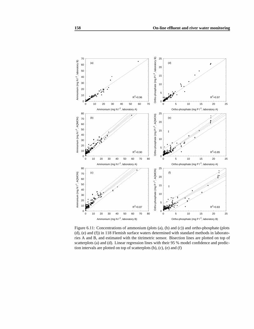
158 On-line effluent and river water monitoring
0
10
20
30
40
50
60
70
0 10 20 30 40 50 60 70
Am
mon
ium
(m
g N
l-1, l
abor
ator
y B
)
Ammonium (mg N l-1, laboratory A)
(a)
R2=0.96
0
10
20
30
40
50
60
70
80
0 10 20 30 40 50 60 70 80
Am
mon
ium
(m
g N
l-1, A
QM
ON
)
Ammonium (mg N l-1, laboratory A)
(b)
R2=0.90
0
10
20
30
40
50
60
70
80
0 10 20 30 40 50 60 70 80
Am
mon
ium
(m
g N
l-1, A
QM
ON
)
Ammonium (mg N l-1, laboratory B)
(c)
R2=0.87
0
5
10
15
20
25
0 5 10 15 20 25
Ort
ho-p
hosp
hate
(m
g P
l-1, l
abor
ator
y B
)
Ortho-phosphate (mg P l-1, laboratory A)
(d)
R2=0.97
0
5
10
15
20
25
0 5 10 15 20 25
Ort
ho-p
hosp
hate
(m
g P
l-1, A
QM
ON
)
Ortho-phosphate (mg P l-1, laboratory A)
(e)
R2=0.85
0
5
10
15
20
25
0 5 10 15 20 25
Ort
ho-p
hosp
hate
(m
g P
l-1, A
QM
ON
)
Ortho-phosphate (mg P l-1, laboratory B)
(f)
R2=0.83
Figure 6.11: Concentrations of ammonium (plots (a), (b) and (c)) and ortho-phosphate (plots(d), (e) and (f)) in 118 Flemish surface waters determined with standard methods in laborato-ries A and B, and estimated with the titrimetric sensor. Bisection lines are plotted on top ofscatterplots (a) and (d). Linear regression lines with their 95 % model confidence and predic-tion intervals are plotted on top of scatterplots (b), (c), (e) and (f)

6.3 Automatic buffer capacity based sensor 159
0
0.5
1
1.5
0 100 200 300 400 500
Soa
p bu
ffer
(mm
ol l-1
)
Chemical oxygen demand (mg COD l-1)
(a)
R2=0.89
0
0.5
1
1.5
0 50 100 150 200
Soa
p bu
ffer
(mm
ol l-1
)Biological oxygen demand (mg BOD l-1)
(b)
R2=0.48
Figure 6.12: Scatterplot of the COD (a) and BOD (b) of 118 Flemish surface waters versus theconcentration of the ‘soap’ component obtained with the buffer capacity sensor
statistically significant (α = 0:01), and the amount of ‘soap’ buffer correlates better with theCOD than with the BOD of surface water samples. It should be mentioned that the variabilityof BOD measurements between and within laboratories is much higher compared to CODmeasurements [69]. On theoretical basis, there should not be a strict relationship betweenbuffer capacities and COD (e.g. sugars have no buffer capacity, but a high COD). Nevertheless,a useful correlation between the ‘soap’ signal and the organic load of a river is established. Asdiscussed above, it is again expected that for one particular sampling point, better correlationscan be obtained when the buffer capacity model is ‘ tuned’ for that location.
Buffer capacity model evaluation
A detailed study of the buffer capacity curves of the effluents and surface waters in relationshipwith their ammonium and ortho-phosphate concentrations was performed, and some observedphenomena were related to the selected buffer capacity model and the model fit. The buffercapacity model of which the model specifications are given in Table 6.3 was fitted to all ex-perimental buffer capacity curves. The experimental and the best-fit simulated buffer capacitycurves of 6 selected surface water samples are given in Figure 6.13. The ammonium andortho-phosphate concentrations found in laboratories A and B, and with the AQMON set-uprespectively are given in Table 6.4.
Example (a) in Figure 6.13 illustrates a typical example of an almost perfect model fit,with a good estimation of ortho-phosphate, but around 80 % overestimation of ammonium.The most probable explanation is the presence of one or more extra buffer systems around pH9�10, that are modelled as ammonium.
Example (b) shows a heavily loaded river water, with a good model fit, and reliable es-timations of ammonium and ortho-phosphate. Some other heavily loaded waters (results notshown) showed a bad model fit, sometimes coupled to wrong estimations mostly of ortho-phosphate (e.g. one dark brown river water with a COD of 2500 mg l�1, had a seven timesoverestimation of ortho-phosphate compared to the laboratory measurements; this particularly
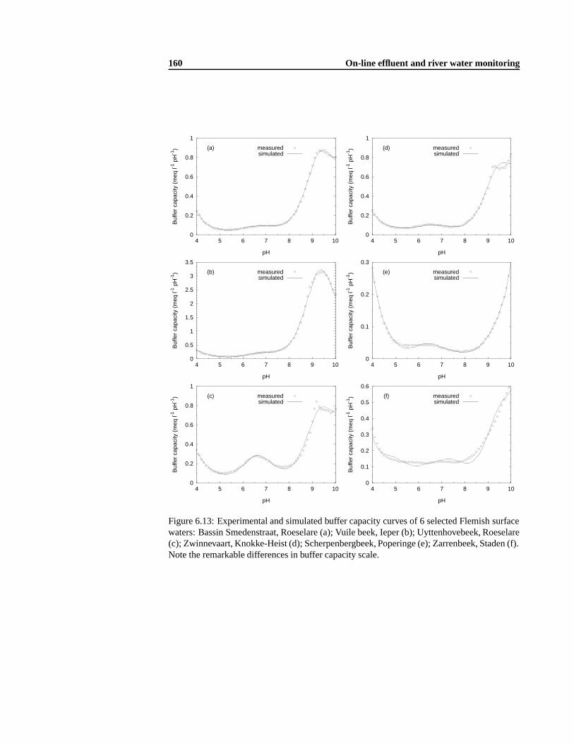
160 On-line effluent and river water monitoring
0
0.2
0.4
0.6
0.8
1
4 5 6 7 8 9 10
Buf
fer
capa
city
(m
eq l-1
pH
-1)
pH
(a) measuredsimulated
0
0.5
1
1.5
2
2.5
3
3.5
4 5 6 7 8 9 10
Buf
fer
capa
city
(m
eq l-1
pH
-1)
pH
(b) measuredsimulated
0
0.2
0.4
0.6
0.8
1
4 5 6 7 8 9 10
Buf
fer
capa
city
(m
eq l-1
pH
-1)
pH
(c) measuredsimulated
0
0.2
0.4
0.6
0.8
1
4 5 6 7 8 9 10
Buf
fer
capa
city
(m
eq l-1
pH
-1)
pH
(d) measuredsimulated
0
0.1
0.2
0.3
4 5 6 7 8 9 10
Buf
fer
capa
city
(m
eq l-1
pH
-1)
pH
(e) measuredsimulated
0
0.1
0.2
0.3
0.4
0.5
0.6
4 5 6 7 8 9 10
Buf
fer
capa
city
(m
eq l-1
pH
-1)
pH
(f) measuredsimulated
Figure 6.13: Experimental and simulated buffer capacity curves of 6 selected Flemish surfacewaters: Bassin Smedenstraat, Roeselare (a); Vuile beek, Ieper (b); Uyttenhovebeek, Roeselare(c); Zwinnevaart, Knokke-Heist (d); Scherpenbergbeek, Poperinge (e); Zarrenbeek, Staden (f).Note the remarkable differences in buffer capacity scale.

6.3 Automatic buffer capacity based sensor 161
Table 6.4: Ammonium and ortho-phosphate concentrations of 6 selected Flemish surface wa-ters determined in laboratories A and B, and with the titrimetric sensor
Figure 6.13 Ammonium (mgN l�1) Ortho-phosphate (mgP l�1)
Subplot Code a lab. A lab. B AQMON lab. A lab. B AQMON
(a) 6260 12.0 9.7 19.3 3.0 2.2 2.4(b) 9740 58.6 65.4 76.7 8.2 8.7 7.7(c) 6230 3.3 3.1 16.9 10.2 11.6 11.8(d) 260 4.5 8.1 15.2 7.2 8.8 2.6(e) 9750 0.4 0.3 1.2 0.2 0.2 0.6(f) 9270 3.0 2.6 9.0 2.8 3.7 6.2
a Identification number of the sampling point, attributed by the VMM.
extreme case corresponds with the two high outlier points in Figure 6.11(e) and (f).Example (c) illustrates a surface water with difficulties for the ammonium estimation. The
buffer capacity around the ammonium buffer had a typical unstable behaviour and the esti-mated ammonium concentration is 5 times too high compared to the laboratory results. Re-markable for this surface water is the high concentration of chlorides (> 500 mgCl l �1). Sim-ilar phenomena were observed in some other samples with high chloride concentrations.
The surface water in example (d) is located near the Northsea and has a very high amountof chlorides (2005 mgCl l�1). The concentration of ortho-phosphate estimated from the buffercapacity profile is rather exceptional because it is three times lower than the laboratory results;this particular case can easily be located as an outlier point in Figure 6.11(e) and (f). Moreover,this sample contained 260 mgCOD l�1, which was one of the highest values in the study. Pos-sibly, some ortho-phosphate remained complexed with other components during titration, andwas thus not available as a buffer around pH 7. One could suggest to introduce ionic strengthcorrections in the buffer capacity model. However, from the graph it can be concluded that itis unlikely that this would have a significant improving effect on the estimated buffer concen-trations, due to the presence of interfering buffers in the neighbourhood of ortho-phosphate.
Example (e) is obtained from a clean river water. The laboratory results indicate that bothammonium and ortho-phosphate are below 1 mg l�1. The model fit is satisfying, except thatthat there is probably an extra buffer present at pH 5.5 which is not accounted for in the buffercapacity model. A typical phenomenon observed in low loaded waters is a relatively large over-estimation of ammonium and ortho-phosphate (a factor 3 in this particular case). This couldbe explained by the higher relative amount of interferences, that are modelled as ammoniumor ortho-phosphate.
Example (f) is the most extreme example where the model fit is not satisfying. The exper-imental buffer capacity profile indicates that more buffer systems are distributed in the con-sidered pH interval, compared to the theoretical buffers included in the buffer capacity modelspecified in Table 6.3. As a consequence, the estimated concentrations of ortho-phosphate andammonium cannot be trusted.

162 On-line effluent and river water monitoring
From detailed visual explorations of the experimental and corresponding simulated buffercapacity profiles of effluents and river waters in relationship with their laboratory analyses, anumber of conclusions can be drawn:
� There is no strict relationship between the goodness of fit and the agreement betweenthe ammonium and ortho-phosphate laboratory analyses and the titrimetric results.
� Examples with a perfect model fit have often good estimations for ammonium and ortho-phosphate, but sometimes suffer from interferences present at the same pKa value of themodelled buffer systems.
� Estimated concentrations of samples with a bad model fit should be interpreted verycarefully. They are mostly suffering from extra interferences compared to well fittingexamples. It could be suggested to use a modified or extended mathematical buffercapacity model in those cases.
Among different evaluated mathematical models (i.e. fixed or variable pKa values, fixed orvariable amount of IC buffer, wide or small simulation interval), the model specified in Table6.3 was found to be the best ‘general purpose’ model. This is an important aspect for field im-plementations, because it is not always possible or realistic to set up preliminary experimentsto define the best site-specific buffer capacity model. In this framework, it was also investigatedwhether it is advantageous with respect to ammonium and ortho-phosphate assessment, to im-plement an automatic buffer capacity model builder (available in the software bombdescribedin section 5.3 on page 117). These results are presented in chapter 9.
6.4 Conclusions
The proposed titration sensor can be used for effluent and surface water monitoring of pHbuffering substances. Experiences with different types of samples have shown that the accu-racy and precision are affected by the composition of the sample. The sensor is capable ofgiving an indication of the ammonium and ortho-phosphate level in the tested effluents andsurface waters. The results in Figures 6.7 and 6.11 illustrate that the variability between thelaboratory analyses and the titrimetric estimations is comparable to the variability between thetwo independent laboratory results.
The buffer capacity at certain pKa’s is suggested to give an indication of the organic load.More particularly, the buffer capacity around pH 5 (named the ‘soap’ buffer) was found to havean useful correlation with the COD of the sample, both for surface waters and effluents.
Due to possible interferences of buffering components and the presence of unmodelledbuffering components in the effluent, this titration sensor cannot be proposed for use as ananalytical instrument. Rather it should be used as an effluent or surface water quality indicatorand detector of possible changes in the sample composition. The titration sensor is suitable forintegration in a robust and reliable automated instrument. An important advantage of the sensoris that no filtration is required. The model database can be easily extended and fully adjustedto particular requirements. The proposed buffer capacity model has been shown to be usefulfor general purposes. However, it is suggested that a site-specific tuning of the mathematicalmodel could offer some perspectives for better and more specific predictions.

6.4 Conclusions 163
The sensor can be used for alarm triggering when the buffer capacity profile changes.However, this should be further investigated and validated with field experiments. This sensorcoupled to an automatic sampler can be used for quality dependent sampling. In this casethe buffer capacity profile is used as a fingerprint for the water composition, and when thefingerprint is changing, a sample is taken for further laboratory analysis. The quality dependentsampling is superior to the time- or flow proportional sampling if such sampling strategy wouldlead to a significantly lower number of laboratory analyses to be performed.

164 On-line effluent and river water monitoring

Chapter 7
Tertiary algal wastewatertreatment monitoring
The results of this chapter were also published in [308].
7.1 Introduction
7.1.1 Algal wastewater treatment
Traditionally, the aims of wastewater treatment have been to reduce the concentration of or-ganic matter and the number of pathogens. However, in many treatment plants typical primaryand secondary treatments cannot meet the increasingly stringent requirements of water pollu-tion control. Although secondary effluents may contain low levels of BOD and COD, they stillcontain high levels of inorganic nutrients (NH+
4 , NO�3 , PO3�
4 ). These nutrients are primarilyresponsible for eutrophication of the receiving waters [147, 230].
Nowadays more and more plants adapt and/or extend their secondary treatment facilitiestowards ‘nutrient removal capacity’ [18, 128, 220], but even effluents with low concentrationsof these pollutants can have a negative impact on the environment if they are discharged in highvolume, especially if the receiving water is a rather small river. Tertiary treatment is becominga necessity to minimize the harmful impact of effluents on the environment.
Besides biological nitrogen and phosphorus removal, numerous physico-chemical treat-ments such as chemical coagulation, breakpoint chlorination, NH3-stripping, reverse osmosisand filtration have been proposed for removing nitrogen and phosphorus. However, due to costsand operational practices, these technologies are not implementable for municipal wastewatertreatment of small communities [151].
As an alternative, tertiary treatment involving micro-algae or cyanobacteria is shown tobe effective in nitrogen and phosphorus removal [147, 151]. The process is quite attractivebecause of its capacity to transform wastes into useful biomass using sunlight as an energysource. However these algal treatment systems also have some drawbacks: The generationtime of the organisms involved is long compared to bacteria; there is a necessity for sunlight;

166 Tertiary algal wastewater treatment monitoring
the active part of the biomass is small and harvesting of biomass is difficult [67, 230].In recent years, research has been conducted to overcome the problems related to algal
tertiary wastewater treatment, and to optimize the treatment process [68, 146, 151, 275, 280].The harvesting problem of the algal biomass has been solved by using organisms like thecyanobacterium Phormidium bohneri, which has the ability to form flocks that settle, thusfacilitating harvest [258].
Algal wastewater treatment processes often are discontinuous, of SBR (sequencing batchreactor) type, where one treatment cycle consists of a filling phase, an aeration phase, a settlingphase and an effluent discharge phase. Such processes need continuous monitoring of the mostimportant process variables, in order to obtain an optimal nutrient removal capacity at minimalcosts. Especially when one realizes that nutrient removal processes are often related to phasesof luxury uptake (e.g. phosphates) and phases of nutrient release, the usefulness of on-linemeasurements is obvious.
7.1.2 Alkalinity related to algal processes
The alkalinity of a water sample is defined as the amount of acid necessary to decrease the pHto a predefined end value. Two end values are considered [104]:
� End value 8.3 (only relevant if the sample pH is higher than 8.3): this is called thephenolphtalein or carbonate alkalinity (symbol C), and is a measure of the amount ofstrong bases, carbonates and alkali present in the sample.
� End value 4.5 (only relevant if the sample pH is higher than 4.5): this is called the totalalkalinity (symbol T), and is a measure of the amount of strong and weak bases (likebicarbonates).
The alkalinity can be measured in the laboratory using a recipient of known volume ofsample and a burette containing a strong acid (e.g. HCl 0.02 N). It can be expressed in meql�1
or in mgCaCO3 l�1.Alkalinity is a popular measurement used in the process control of diverse water treat-
ment processes, e.g. in activated sludge treatment [249, 256, 283] or in anaerobic wastewatertreatment [46, 71]. In practice alkalinity is often used as a practical measure of the amount ofcarbonates and bicarbonates in the water. There are some particular remarks concerning theuse of alkalinity as ‘ (bi)carbonate’ estimator:
� In cases the sample is loaded with weak acid buffering systems other than the CO2
subsystem (like ammonium, phosphates and VFA’s), these components will be includedin the alkalinity and will suggest that more (bi)carbonates are present than in reality [65].
� For the pH meter method, it is advised to choose the end value in function of the alka-linity (end-value ranging from pH 4.3 to pH 4.9 for high to low alkalinity respectively)[281]. For colour indicator methods, like the bromcresol method, the pH value 4.5 cor-responds with the inflection point on the titration curve where the colour indicator willswitch to its other state. In case the inflection point is not so sharp, or the solutioncontains strong colouring substances, the colour switch will be difficult to observe. Forthis reasons, the pH meter method is mostly preferred above the older colour indicatormethods.

7.1 Introduction 167
In the application area of wastewater treatment, modified or extended methods of the alka-linity measurement have been developed. Examples of extended methods where more than 1end value in the titration profile are considered are a three-point method [12] and a five-pointmethod [197] for the determination of bicarbonate and VFA. Methods using more than 5 pointsfor bicarbonate and VFA estimation have also been developed [36, 228]. To eliminate the ef-fect of interfering pH buffers when one is only interested in bicarbonate content, a methodwas developed where the CO2 is stripped from the sample by addition of strong acid. Thestripped CO2 can be directly measured by the volumetric [108, 111] or pressure [71] build-upof CO2. The described methods have been used in the application area of anaerobic treatment,where high concentrations of both bicarbonate and VFA’s are present [46, 65]. An overview ofmeasurement methods for CO2 and bicarbonate is given in [75, 219].
Alkalinity related techniques for bicarbonate estimation are well developed in applicationswhere CO2 is continuously generated by micro-organisms degrading organics. In these areaspossible interferences with other pH buffering components are negligible. In the area of algaltreatment, on the other hand, CO2 is consumed by the algae, resulting in relatively low or evenlimiting concentrations of bicarbonate in the water samples. Inorganic carbon (IC) is of majorimportance, because it is the only carbon source used by algae. Among the different forms ofIC (CO2(aq), HCO�
3 and CO2�3 ), only the two first ones are taken up by the algal biomass, and
thus useful as a carbon substrate [80, 97, 278]. The preference for CO2(aq) or HCO�3 uptake
is pH dependent [286] and an adaptation period to switch between the CO2(aq) and HCO�3
transport system may be required [80]. The importance of the IC buffer system in relation tophotosynthetic algal growth is widely described in literature [199, 259, 277, 279]. Therefore,the usefulness of quantifying the IC buffer for algal wastewater treatment is twofold. First,a precise knowledge of the inorganic carbon content can indicate whether the IC becomeslimiting [199], and whether IC supply is needed [259, 279]. Second, because IC is the onlycarbon source used by the algae, the rate of IC consumption under light conditions can be usedas a process and control variable, e.g. indicating a possible reactor failure if the IC consumptionis too low.
7.1.3 Objectives
The objective of this chapter is to develop a pH buffer capacity based sensor, capable of extract-ing concentrations of pH buffering components from on-line measured titration curves comingfrom the influent, effluent and reactor content of an algal pilot plant. The information thatcan be extracted from the buffer capacity profiles using mathematical modelling is evaluatedtowards its usefulness related to tertiary algal treatment processes. The relationship betweenthe alkalinity and the IC buffer capacity will be discussed, as well as the ammonium and ortho-phosphate assessment from the buffer capacity profile. In the latter case, IC, NH+
4 and o-PO4
will be incorporated in equation (3.59) on page 49 as diprotic, monoprotic and triprotic weakacids respectively. The results obtained with the buffer capacity sensor seem promising asinput to develop a control strategy, although this is not the objective of this chapter.

168 Tertiary algal wastewater treatment monitoring
7.2 Materials and Methods
7.2.1 The algal pilot plant
A pilot reactor with algal biomass, installed at the outlet of the activated sludge plant Valcartiernear Quebec city (Canada), was used for the sample collection between July 22 and August12, 1997. The activated sludge plant was treating domestic wastewater of the military baseValcartier, and received an influent flow of around 2500 m3d�1. The plant was operating inpartially nitrifying mode and the secondary effluent nitrogen was present in two forms, NH+
4and NO�
3 .The algal bioreactor with a triangular cross-section had a volume of 6 m3 and combined
aeration and mixing was obtained by means of a perforated flexible tube at the bottom of thereactor. This pilot reactor was in use for 2 years and its function was to further decrease thenutrient concentrations of the secondary effluent. The reactor was used in batch mode, in cyclesof 1 or 2 days. A cycle consisted of a filling phase (in the morning), an aeration phase of 12 or36 hours, a sedimentation phase (at night) to allow the algae to settle down, and a decantationphase (in the morning) to remove an upper liquid layer of around 75 % of the total reactorvolume. The biomass concentration in the reactor was kept between 100 and 600 mg DW l�1.
7.2.2 Sampling and laboratory measurements
Light, pH, DO and temperature were monitored continuously in the algal pilot plant. Threedifferent kinds of samples were taken for further analysis in the laboratory:
� The Effluent of the ValCartier plant (sample code EVC), being the influent of the algalpilot reactor;
� The content of the Algal Pilot (sample code AP), 3 hours after the reactor was filled andcompletely mixed by the aeration;
� The Effluent of the Algal Pilot plant (sample code EAP).
The EVC and EAP samples were taken with a peristaltic pump in the inlet and outlet of thepilot plant during filling and decantation phases respectively. The AP samples were taken asmanual grab samples. All samples were stored immediately in the fridge (4 oC) and processedin the laboratory within 1 day.
Prior to the laboratory analyses (NH+4 , NO�
3 , o-PO4), all samples were filtered on a What-man 934 AH filter, with a pore size of 1.5 µm. The analyses were conducted according toStandard Methods [104]. For the total alkalinity measurements in the laboratory, the pH metermethod was used [104].
7.2.3 Titration curves
Titrations were performed with a laboratory titrator (Metrohm Titrino 716 [168]). Data ac-quisition was performed with a 386 PC connected to the titrator. The titrated sample volumewas 100 ml, and titration took place in a completely closed magnetically stirred titration vesselcontaining a CO2 scrubber (bowed glass tube with soda lime pellets) to prevent entrance ofCO2 from the air. The headspace of the titration vessel was 150 ml. Prior to titration, the

7.2 Materials and Methods 169
refrigerated samples were equilibrated to 25 oC with a warm water bath, and they were imme-diately titrated at room temperature, which varied between 20 and 25 oC. Two different typesof titration profiles were collected:
Down titration profile: The sample as such was titrated with 0.1 N HCl from the actual pHto pH 2.5 using a monotonic end-point titration (MET) method [168], with fixed stepsof 0.05 ml. This type of titration was used for the determination of the IC buffer.
Up titration profile: The down titrated sample was strongly agitated with a magnetic stirrerfor 15 minutes to remove all CO2, while the titration vessel was open to the air. Next,the vessel was closed and the sample was titrated with 0.1 N NaOH to pH 11 using adynamic end-point titration (DET) method [168]. The difference with the MET methodis that the DET method does not take fixed volume steps, but variable volume steps(small versus big steps when the buffer capacity is low or high respectively). This typeof titration was used for the determination of ammonium and ortho-phosphate.
7.2.4 Data processing software
The software bomb, described in section 5.3 on page 117, was used for the calculation of thebuffer capacity profiles. Such a profile is the inverse of the first derivative of the titration pro-file. The calculation of the derivative was performed using a parabolic regression in a movingwindow of 5 experimental data points of the titration curve. No further smoothing algorithmswere necessary to obtain a smooth buffer capacity profile. The same software was used tofit several mathematical models to the calculated buffer capacity curve. The mathematicalmodel specifications were defined in a special input file, read by the program. The softwarewas running on an INDIGO workstation (Silicon Graphics, U.S.) and the data processing of 1experimental data file needed approximately 1 minute.
7.2.5 Mathematical models
The mathematical models used were all based on the general buffer capacity equation (3.59)on page 49. For each model used, the following considerations were taken into account:
� The pH interval used for data processing.� Which pH buffering components to be included in the model.� The initial guesses for the concentrations and pKa values.� Which concentrations and pKa values had to be adjusted in order to fit the simulation
model to the experimental data. The parameters that are to be estimated are specifiedwith a lower and upper limit (constrained optimization). The reason for optimizing pKa
values instead of keeping them fixed at the pK0a or another value is to take into account
the residual effects of temperature, ionic strength and possible electrode errors on theposition of the pKa values in the experimental buffer capacity curve.
For the down titrations a simulation interval between pH 4 and pH 7.3 was taken. Evenif the initial pH of the sample was much higher than 7.3, it was not worthwhile to extendthe simulation interval and incorporate ortho-phosphate or ammonium in the model, becausethe magnitude of the IC buffer would interfere with the other smaller buffer systems. For

170 Tertiary algal wastewater treatment monitoring
Table 7.1: Down titration model specifications for a simulation between pH 7.3 and pH 4
Buffer Variable Initial guess or value Estimated? Lower limit Upper limit
Water pka water 15.74 Noconc water 55.5 mol l�1 No
IC pka1 carbon 6.37 Yes 6 7pka2 carbon 10.25 Noconc carbon 1 meqIC l�1 Yes 0 2.5
Soap pka soap 4.8 Yes 4 5.5conc soap 5 10�5 mol l�1 Yes 0 1 10�3
the up titrations, a simulation interval between pH 4 and pH 10 was chosen. In the software,concentrations can be specified in mol l�1 or mg l�1. More detailed model specifications forthe down and up titrations are shown in Table 7.1 and Table 7.2 respectively. The ‘soap’term in the models stands for a range of components that all have a buffer capacity in therange between pH 4 an pH 5.5, e.g. numerous organic acids. The ‘blank1’ term representsan unknown buffering component around pH 10, found to be present in almost all samplesanalyzed. The reason for incorporating the ‘carbon’ component in the up titration model,despite the fact that the sample is made CO2 free, is that during up titration the CO2 initiallypresent in the headspace above the vessel, or small amounts of CO2 present in the titrant, canenter the sample and typically account for 0.07 meqIC l�1.
Furthermore, once the total concentration CIC (which is [CO2�3 ]+ [HCO�
3 ]+ [CO2(aq)]) isdetermined using the simulation model, the partitioning of these 3 forms can be calculated asfunction of the actual pH [281]. Using the mass balance and the 3 equilibrium equations forIC, the concentrations [CO2(aq)], [HCO�
3 ] and [CO2�3 ] are given by equations (7.1), (7.2) and
(7.3) respectively. Details on obtaining these equations can be found in [273, 281].
[CO2(aq)] =10�2pH
10�2pH+10�(pH+pKa1)+10�(pKa1+pKa2)CIC (7.1)
[HCO�3 ] =
1� 10�2pH +10�(pKa1+pKa2)
10�2pH+10�(pH+pKa1)+10�(pKa1+pKa2)
!CIC (7.2)
[CO2�3 ] =
1� 10�2pH+10�(pH+pKa1)
10�2pH+10�(pH+pKa1)+10�(pKa1+pKa2)
!CIC (7.3)
It is important to remark that the latter 3 equations are valid only in a completely closed andequilibrated system. As the algal reactor is an open system, the concentration of CO2(aq) isalso driven by Henry’s law [260]:

7.3 Results and Discussion 171
Table 7.2: Up titration model specifications for a simulation between pH 4 and pH 10
Buffer Variable Initial guess or value Estimated? Lower limit Upper limit
Water pka water 15.74 Noconc water 55.5 mol l�1 No
IC pka1 carbon 6.37 Nopka2 carbon 10.25 Noconc carbon 0.07 meqIC l�1 Yes 0 0.25
o-PO4 pka1 phos 2.15 Nopka2 phos 7.21 Yes 7 7.8pka3 phos 12.35 Noconc phos 3 mgP l�1 Yes 0 30
NH+4 pka ammon 9.25 Yes 9 9.5
conc ammon 2 mgN l�1 Yes 0 30Soap pka soap 4.8 Yes 4 5.5
conc soap 5 10�5 mol l�1 Yes 0 1 10�3
Blank1 pka blank1 9.6 Yes 9.4 11.5conc blank1 5 10�5 mol l�1 Yes 0 1 10�3
[CO2(aq)] = KH � pCO2(air)(7.4)
With KH = 3:4 10�2 M atm�1 (at T = 25 oC) and pCO2(air)= 3 10�4 atm, equation (7.4) leads
to an air/liquid equilibrium concentration of [CO2(aq)] = 10�5M or 0.01 meq l�1, which is avery low value. Furthermore, one has to take into account that a biological active system likeand algal system is quite seldom in equilibrium with the atmosphere [37], so careful use ofequation (7.4) is advised.
7.3 Results and Discussion
7.3.1 Alkalinity and IC buffer capacity
A random sample from the algal pilot reactor AP, taken in the morning of a sunny day wasanalyzed with the titrator and in the laboratory. A filtered and an unfiltered sample were titratedfrom the actual pH to pH 2.5 (Figure 7.1). Both samples were also analyzed on the totalalkalinity with two standard methods. From the titration curves, the corresponding buffercapacity curves (Figure 7.2) were calculated and the simulation model (equation (3.59) onpage 49 and Table 7.1) was used to quantify the concentration of the IC buffer. The best fitsimulation result for the unfiltered and filtered sample is given in Figure 7.2.
For the total alkalinity determination, the end-point pH value for the pH meter method was

172 Tertiary algal wastewater treatment monitoring
2
3
4
5
6
7
8
9
10
0 0.2 0.4 0.6 0.8 1 1.2 1.4 1.6 1.8 2
pH
ml HCl 0.12 N added
unfiltered samplefiltered sample
Figure 7.1: Titration curves of an unfiltered and filtered AP sample
0
0.1
0.2
0.3
0.4
0.5
0.6
4 5 6 7 8 9
Buf
fer
capa
city
(m
eq l-1
pH
-1)
pH
unfiltered sample
filtered sample
Figure 7.2: Measured (points) and simulated (lines) buffer capacity curves of an unfiltered andfiltered AP sample

7.3 Results and Discussion 173
Table 7.3: Alkalinity measurements and IC simulation results
Filtered sample Unfiltered samplemeq l�1 meq l�1
Total alkalinity (pH meter method [104]) 1.09 1.17
Total alkalinity from titration curve (T) 1.11 1.20Carbonate alkalinity from titration curve (C) 0.15 0.15(T�C) alkalinity from titration curve 0.96 1.05(T�2C) alkalinity from titration curve 0.81 0.90
Simulated CIC from titration curve 0.80 0.85Simulated [HCO�
3 ] using equation (7.2) 0.75 0.80
set at pH 4.5, according to the standard method [104]. This method was also applied to thetitration curves of Figure 7.1, where an interpolation between 2 successive data points was usedto make a reading of the amount of acid necessary to bring the pH to 8.3 and 4.5 respectively.For comparison reasons, the simulation results to quantify the IC buffer were also expressedas meq l�1.
The results of the alkalinity measurements and the simulation results for IC are presentedin Table 7.3. The precision of the total alkalinity measurements (both the pH meter method andfrom the titration curve), expressed as relative standard deviation (r.s.d.), was between 1 and 2%. The r.s.d. of the simulated IC concentration based on down titration profiles was 2 %. Onecan notice that the results for the filtered sample are only about 7 % lower than the unfilteredsample. This means that the alkalinity or IC buffer capacity is mainly related to the solublephase and not to the algal biomass phase. The total alkalinity with the standard pH metermethod was not significantly different from the total alkalinity calculated from the titrationcurves in Figure 7.1 (t-test; α = 0:05). An interesting feature of this experiment is found whencomparing the IC content found with the modelled buffer capacity curves and the alkalinitycalculated from the same experimental titration curve. From Table 7.3, it can be seen that thetotal alkalinity is about 40 % higher than the corresponding simulated IC concentration andthat the (T�C) alkalinity is still more than 20 % higher than the simulated IC concentration.This is the case in both the filtered and unfiltered sample. This indicates that the alkalinity ofthe sample is mainly, but not completely determined by the amount of IC.
To make a further interpretation of the different results in Table 7.3, a summarizing ta-ble with the buffers that are included in these results is presented in Table 7.4. None of themeasurements in Table 7.4 exactly represents the amount of CO2(aq) or HCO�
3 in the water,which are the only two IC species that are available to the algae. The IC obtained with thesimulation model will be the closest to the real amount of IC because interferences in the pHrange 7 or higher (ammonium, ortho-phosphate) and in the pH range of 5.5 and lower (organicacids, detergents) are excluded in the simulation method. For the sample studied, the initialpH was 9.1, and the partitioning between the 3 different carbon species was 0.2 % CO2(aq),

174 Tertiary algal wastewater treatment monitoring
Table 7.4: Different buffers that are included in the alkalinity measurements and IC simulationresults (assuming actual pH of sample > 8.3)
Measurement Buffers that are included in the measurement
Total alkalinity (T) 2CO2�3 +HCO�
3 + other buffers between actual pH and pH 4.5Carbonate alkalinity (C) CO2�
3 + other buffers between actual pH and pH 8.3(T�C) alkalinity CO2�
3 +HCO�3 + other buffers between pH 8.3 and pH 4.5
(T�2C) alkalinity HCO�3 + other buffers between pH 8.3 and pH 4.5
� other buffers between actual pH and pH 8.3
Simulated CIC CO2�3 +HCO�
3 +CO2(aq) + buffers with pKa: � pKa: of ICSimulated [HCO�
3 ] HCO�3 + other buffers with pKa: � pKa1 of IC
93.9 % HCO�3 and 5.9 % CO2�
3 , calculated with equations (7.1), (7.2) and (7.3) respectively.From this, it is concluded that the algal available carbon was mainly in the bicarbonate form.From Table 7.4, it can be concluded, that in case the only buffer in the sample is the IC buffer,then both (T�2C) and the simulated [HCO�
3 ] represent exactly the bicarbonate content. If alsoother buffer systems (ammonium, ortho-phosphate, organic acids, : : : ) are present in the sam-ple, the situation is different. On the one hand, the simulated [HCO�
3 ] will overestimate thereal bicarbonate content when extra buffers with the same pKa: as the pKa1 of IC are present.On the other hand, the bicarbonate assessment from the (T�2C) measurement will be influ-enced by a much wider range of buffers. All extra buffers between pH 8.3 and pH 4.5 (e.g.ortho-phosphate, organic acids) will lead to an overestimation of the bicarbonate content, andall extra buffers between the actual pH and pH 8.3 (e.g. ammonium) will lead to an underes-timation of the bicarbonate content. Practically, in this example, when comparing the (T�2C)to the simulated [HCO�
3 ] for bicarbonate estimation, an overestimation of the real amount ofbicarbonate by (T�2C) is minimal 8 and 12 % for the filtered and unfiltered samples respec-tively (concluded from Tables 7.3 and 7.4 together). From 36 unfiltered samples (pH between7.1 and 9.1) taken at various times in the algal reactor, it was found that the (T�2C) mea-surement always gave 4 to 22 % overestimation of the bicarbonate content compared to the[HCO�
3 ] from the simulation method. In case the IC would become more limiting in the algalreactor, or the interfering buffers would become more pronounced, the simulation method isto be preferred by far for the determination of available bicarbonate for the algae. Besides, theresult of the simulation method does not depend on the choice of the end-point (pH 4.3 to 4.9,depending on the method and alkalinity range).
For this particular case-study, an automated alkalinity measurement possibly would revealsimilar process information as the IC determination with the buffer capacity sensor. However,because the hardware and the hardware related practical difficulties (maintenance, calibration,: : : ) of an automated alkalinity measurement are very similar to this buffer capacity sensor,the main advantage of the buffer capacity sensor is that more parameters are obtained with asingle measurement device.

7.3 Results and Discussion 175
7.3.2 Ammonium and ortho-phosphate evaluation in grab samples
During a period of 14 days, samples were taken in the influent of the algal pilot reactor (EVC),in the reactor itself (AP) and in the effluent of the algal pilot plant (EAP). These samples wereanalyzed in the laboratory for NH+
4 and o-PO4. Subsamples of 100 ml were used to perform uptitrations to obtain the buffer capacity profiles. For the AP samples, containing algal biomass,2 different titration experiments were performed:
� Titration of the raw sample as such (including 100 to 600 mg DW l�1 of the algae);� Titration of the supernatant after the algae were settled.
After the titration data were collected, the data processing was performed. The repro-ducibility for repeated sampling, titrating and optimization, expressed as relative standard de-viation (r.s.d.), was less than 2 % for the ammonium concentration and less than 5 % for theortho-phosphate concentration. The results of the AP samples with or without biomass werecomparable for the ammonium prediction but different for the ortho-phosphate prediction. Forthe o-PO4, the samples with biomass gave 50 to 100 % higher values than the samples withoutthe biomass. This might indicate that a considerable amount of phosphate is related to thebiomass fraction, or that this biomass fraction contains other weak acid buffering systems thatinterfere with the titrimetric ortho-phosphate determination. The validity range of the measure-ments using this approach is case dependent (e.g. presence or absence of interfering buffers)and depends on the titration conditions (e.g. sample volume, titrant normality, measurementpoint density). Based on the experience for this particular case, the minimum validity valuesare considered around 1 mgN l�1 and 1 mgP l�1.
Using the mathematical model (equation (3.59) on page 49) and Table 7.2), a perfect fit be-tween the experimental and simulated buffer capacity curves was obtained for all experimentaldata. An illustration of the experimental data and the model fitting for 3 selected EAP samplestaken at different days is illustrated in Figure 7.3. On the graph, one can easily distinguishthe profiles of samples that are high or low in ammonium and/or phosphate concentration. Forthe samples shown in Figure 7.3, together with the other grab samples, the laboratory mea-surements of NH+
4 and o-PO4 and the concentrations estimated with the model (titrator) arepresented in Table 7.5. For the AP samples, only the results of the titration experiments withoutthe algal biomass are shown, because they correspond most closely to the laboratory procedurewhere all samples were filtered prior to analysis. Overall, the linear relationship between lab-oratory and titrator results is shown in Figures 7.4 and 7.5. The constructed linear regressionlines with their 95 % confidence intervals are comparable to the results obtained in chapter 6on secondary effluents with a similar buffer capacity sensor.
7.3.3 Dynamic nutrient evolution in a 48 hour batch experiment
A 48 hour batch experiment was set up to monitor the nutrient removal in the algal pilot plant.The experiment started with a filling phase with EVC water at 08:00 in the morning. In the first36 hours of the experiment, the aeration was activated, ensuring a completely mixed reactor.During the last 12 hours, the aeration was stopped. An automatic time-proportional samplerwas used to obtain combined samples every 3 hours. During this experiment, 19 samples weretitrated, among which the first 11 were samples from a completely mixed system (when aera-tion was activated). The last 8 samples were taken during the second night of the experiment,

176 Tertiary algal wastewater treatment monitoring
0
0.1
0.2
0.3
0.4
0.5
0.6
4 5 6 7 8 9 10
Buf
fer
capa
city
(m
eq l-1
pH
-1)
pH
July 30, 1997
August 5, 1997
August 8, 1997
Figure 7.3: Measured (points) and simulated (lines) buffer capacity curves for 3 selected EAPsamples
Table 7.5: Laboratory measurements and simulation results for all grab samples
NH+4 (mgN l�1) o-PO4 (mgP l�1)
Sample Date laboratory titrator laboratory titrator
EVC July 30, 1997 4.6 9.0 3.4 3.2August 5, 1997 21 23 3.7 3.1August 6, 1997 19.6 21 3.9 3.4August 8, 1997 15.2 18.6 4.3 3.5
EAP July 30, 1997 0.6 0.8 3.8 2.1August 5, 1997 0.8 1.0 1.2 1.2August 6, 1997 9.4 10.8 4.2 3.4August 8, 1997 12 13.4 3.9 2.9
AP August 4, 1997 2.8 2.7 3.3 2.7August 5, 1997 13.2 14.6 4.6 3.9August 6, 1997 16.9 19.5 4.3 3.6August 8, 1997 14.3 16.9 4.1 3.6August 12, 1997 13 9.3 3.2 3.0

7.3 Results and Discussion 177
0
5
10
15
20
25
0 5 10 15 20 25
NH
4 tit
rato
r (m
g N
l-1)
NH4 lab (mg N l-1)
R2=0.93
EVCEAP
AP0.68 + 1.06 NH4-N lab
95% model confidence interval
Figure 7.4: Scatterplot of laboratory and titrator ammonium results for all grab samples
0
1
2
3
4
5
0 1 2 3 4 5
o-P
O4
titra
tor
(mg
P l-1
)
o-PO4 lab (mg P l-1)
R2=0.76
EVCEAP
AP0.32 + 0.74 o-PO4-P lab
95% model confidence interval
Figure 7.5: Scatterplot of laboratory and titrator ortho-phosphate results for all grab samples
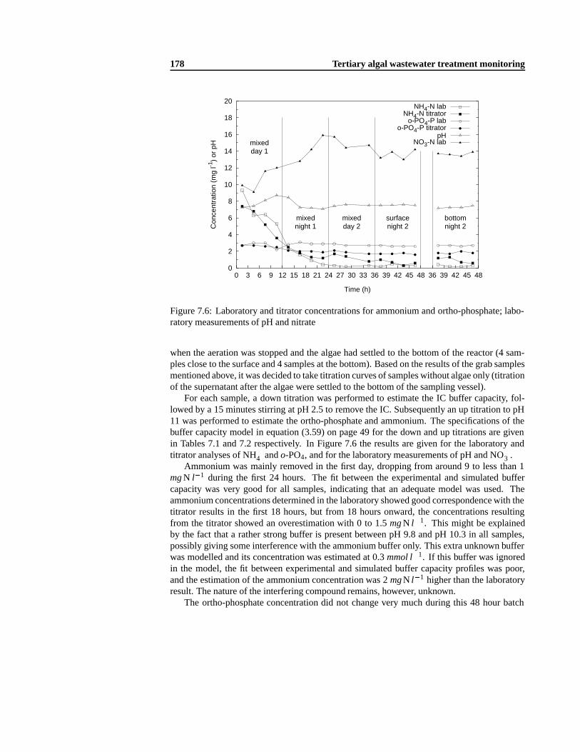
178 Tertiary algal wastewater treatment monitoring
0
2
4
6
8
10
12
14
16
18
20
0 3 6 9 12 15 18 21 24 27 30 33 36 39 42 45 48 36 39 42 45 48
Con
cent
ratio
n (m
g l-1
) or
pH
Time (h)
mixedday 1
mixednight 1
mixedday 2
surfacenight 2
bottomnight 2
NH4-N labNH4-N titrator
o-PO4-P labo-PO4-P titrator
pHNO3-N lab
Figure 7.6: Laboratory and titrator concentrations for ammonium and ortho-phosphate; labo-ratory measurements of pH and nitrate
when the aeration was stopped and the algae had settled to the bottom of the reactor (4 sam-ples close to the surface and 4 samples at the bottom). Based on the results of the grab samplesmentioned above, it was decided to take titration curves of samples without algae only (titrationof the supernatant after the algae were settled to the bottom of the sampling vessel).
For each sample, a down titration was performed to estimate the IC buffer capacity, fol-lowed by a 15 minutes stirring at pH 2.5 to remove the IC. Subsequently an up titration to pH11 was performed to estimate the ortho-phosphate and ammonium. The specifications of thebuffer capacity model in equation (3.59) on page 49 for the down and up titrations are givenin Tables 7.1 and 7.2 respectively. In Figure 7.6 the results are given for the laboratory andtitrator analyses of NH+
4 and o-PO4, and for the laboratory measurements of pH and NO�3 .
Ammonium was mainly removed in the first day, dropping from around 9 to less than 1mgN l�1 during the first 24 hours. The fit between the experimental and simulated buffercapacity was very good for all samples, indicating that an adequate model was used. Theammonium concentrations determined in the laboratory showed good correspondence with thetitrator results in the first 18 hours, but from 18 hours onward, the concentrations resultingfrom the titrator showed an overestimation with 0 to 1.5 mgN l�1. This might be explainedby the fact that a rather strong buffer is present between pH 9.8 and pH 10.3 in all samples,possibly giving some interference with the ammonium buffer only. This extra unknown bufferwas modelled and its concentration was estimated at 0.3 mmol l�1. If this buffer was ignoredin the model, the fit between experimental and simulated buffer capacity profiles was poor,and the estimation of the ammonium concentration was 2 mgN l�1 higher than the laboratoryresult. The nature of the interfering compound remains, however, unknown.
The ortho-phosphate concentration did not change very much during this 48 hour batch
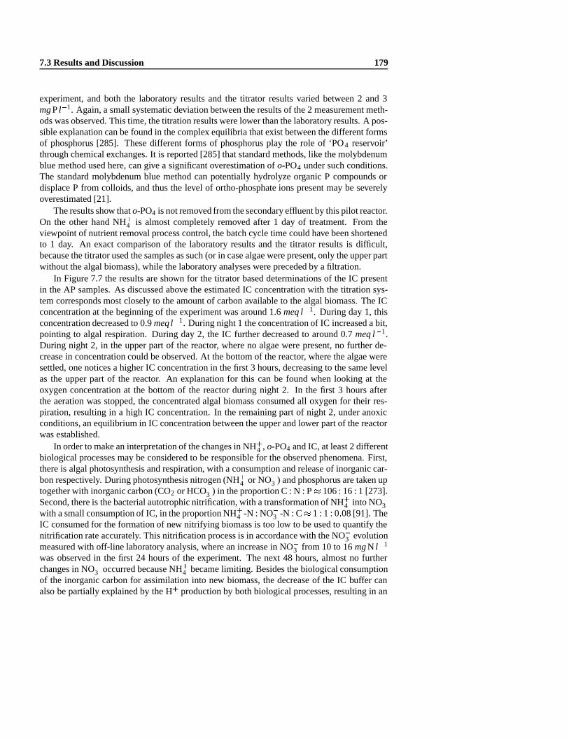
7.3 Results and Discussion 179
experiment, and both the laboratory results and the titrator results varied between 2 and 3mgP l�1. Again, a small systematic deviation between the results of the 2 measurement meth-ods was observed. This time, the titration results were lower than the laboratory results. A pos-sible explanation can be found in the complex equilibria that exist between the different formsof phosphorus [285]. These different forms of phosphorus play the role of ‘PO 4 reservoir’through chemical exchanges. It is reported [285] that standard methods, like the molybdenumblue method used here, can give a significant overestimation of o-PO4 under such conditions.The standard molybdenum blue method can potentially hydrolyze organic P compounds ordisplace P from colloids, and thus the level of ortho-phosphate ions present may be severelyoverestimated [21].
The results show that o-PO4 is not removed from the secondary effluent by this pilot reactor.On the other hand NH+
4 is almost completely removed after 1 day of treatment. From theviewpoint of nutrient removal process control, the batch cycle time could have been shortenedto 1 day. An exact comparison of the laboratory results and the titrator results is difficult,because the titrator used the samples as such (or in case algae were present, only the upper partwithout the algal biomass), while the laboratory analyses were preceded by a filtration.
In Figure 7.7 the results are shown for the titrator based determinations of the IC presentin the AP samples. As discussed above the estimated IC concentration with the titration sys-tem corresponds most closely to the amount of carbon available to the algal biomass. The ICconcentration at the beginning of the experiment was around 1.6 meq l�1. During day 1, thisconcentration decreased to 0.9 meql�1. During night 1 the concentration of IC increased a bit,pointing to algal respiration. During day 2, the IC further decreased to around 0.7 meq l�1.During night 2, in the upper part of the reactor, where no algae were present, no further de-crease in concentration could be observed. At the bottom of the reactor, where the algae weresettled, one notices a higher IC concentration in the first 3 hours, decreasing to the same levelas the upper part of the reactor. An explanation for this can be found when looking at theoxygen concentration at the bottom of the reactor during night 2. In the first 3 hours afterthe aeration was stopped, the concentrated algal biomass consumed all oxygen for their res-piration, resulting in a high IC concentration. In the remaining part of night 2, under anoxicconditions, an equilibrium in IC concentration between the upper and lower part of the reactorwas established.
In order to make an interpretation of the changes in NH+4 , o-PO4 and IC, at least 2 different
biological processes may be considered to be responsible for the observed phenomena. First,there is algal photosynthesis and respiration, with a consumption and release of inorganic car-bon respectively. During photosynthesis nitrogen (NH+
4 or NO�3 ) and phosphorus are taken up
together with inorganic carbon (CO2 or HCO�3 ) in the proportion C : N : P� 106 : 16 : 1 [273].
Second, there is the bacterial autotrophic nitrification, with a transformation of NH+4 into NO�
3with a small consumption of IC, in the proportion NH+
4 -N : NO�3 -N : C� 1 : 1 : 0:08 [91]. The
IC consumed for the formation of new nitrifying biomass is too low to be used to quantify thenitrification rate accurately. This nitrification process is in accordance with the NO�
3 evolutionmeasured with off-line laboratory analysis, where an increase in NO�
3 from 10 to 16 mgN l�1
was observed in the first 24 hours of the experiment. The next 48 hours, almost no furtherchanges in NO�
3 occurred because NH+4 became limiting. Besides the biological consumption
of the inorganic carbon for assimilation into new biomass, the decrease of the IC buffer canalso be partially explained by the H+ production by both biological processes, resulting in an

180 Tertiary algal wastewater treatment monitoring
0.5
1
1.5
2
0 3 6 9 12 15 18 21 24 27 30 33 36 39 42 45 48 36 39 42 45 48
Con
cent
ratio
n (m
eq l-1
)
Time (h)
mixed
day 1
mixed
night 1
mixed
day 2
surface
night 2
bottom
night 2
IC titrator
Figure 7.7: Titrator concentrations for inorganic carbon
alkalinity decrease [273]. On the other hand, the algal uptake of dissolved CO2 during day-time, resulted in a net pH increase from pH 7.3 to pH 8.7, as observed during the first 12 hours.The pH of all samples was between pH 7.1 and pH 8.7, meaning that the bio-available carbonwas always higher than 95 % of the quantified IC buffer system (equations (7.1) and (7.2)). Inthis case study, the IC never dropped below 0.7 meql�1, which is a rather safe value comparedto the 0.5 meq l�1 reported to be needed [199] for normal operation. From an industrial pointof view, this algal wastewater treatment appears to be a viable alternative for small communi-ties [151]. However, the pilot-plant experiments in this study have shown that especially forthe phosphate removal, the % P removed (by precipitation and/or biologically) is lower thanprevious, smaller-scale studies [146, 230]. In the viewpoint of possible eutrophication of thereceiving waters, further insights in the phosphorus removal mechanisms and further processoptimization are necessary. The role of phosphorus in the eutrophication of receiving waters iscomplex because phosphorus is a very dynamic, biologically active element [54, 59].
As the results of the titration method can be influenced by interfering buffering compo-nents, this measurement method cannot be considered to be an analytical device, replacing thestandard laboratory methods. As illustrated above, the application of this titration method hasto be seen in the context of process monitoring and alarm generation. An innovative aspect ofthe presented buffer capacity sensor, is that it gives a multivariate response (IC, NH+
4 , o-PO4)supplemented with extra information, e.g. the appearance or disappearance of extra buffersystems, that are useful for process monitoring.
Further research will focus on the implementation of a fully automatic sensor, includingautomatic buffer model selection to accommodate for (dis)appearing buffer systems. Further,an appropriate control strategy will be developed in which this device is providing the neces-sary data in due time. The time needed to perform a full measurement cycle was approximately

7.4 Conclusions 181
1 hour (down titration, up titration and data interpretation). Further optimization of the titra-tion parameters can reduce this cycle time with 10�20 minutes. The cycle time can be furtherdecreased to 20� 25 minutes if the down and up titrations are performed in parallel titrationvessels. Electrode problems were never observed during the performed experiments. Themaintenance of the titration vessel and electrode is comparable to the maintenance of a pHmeter.
7.4 Conclusions
The proposed methodology of a pH buffer capacity based measurement system was evaluatedfor its usefulness for multivariate monitoring of tertiary wastewater treatment with algae. Inwaters which are low or even limiting in IC buffer capacity (like in algal treatment plants),standard alkalinity measurements can give an overestimation of the IC buffer system, becausethe alkalinity is a general composite measurement, including all pH buffering componentsin the considered pH interval. For the samples analyzed, the (T�C) alkalinity was around20 % higher than the IC concentration obtained with the buffer capacity sensor, explainingthat other buffering components than IC are included in the (T�C) alkalinity (o-PO4, NH+
4 ,organic acids, : : : ). It is concluded that the HCO�
3 concentration assessed with the simulationmethod is preferred, rather than the (T�2C) alkalinity, when one wants to quantify the availablebicarbonate.
The NH+4 and o-PO4 assessment from the up titration profiles were comparable with the
laboratory measurements. An exact comparison of the laboratory results and titration resultswas difficult, because of the filtration step preceding laboratory analyses, and possible inter-ferences by buffer systems not accounted for in the model.
During a 48 hours batch experiment, the measured IC concentration reflected the day/nightdifference in activity of the algal biomass fairly well. The data of the titrimetric sensor showedthat there was no carbon limitation and that the treatment cycle could have been halved to 24hours, still allowing complete NH+
4 -removal. The IC reduction rate during daytime was anindicator of the biological activity.
The application of the sensor developed here has to be seen in the context of process mon-itoring and alarm generation. The developed methodology can be realistically implemented inan on-line automatic measurement system. The sensor does not need any sample filtration, amajor advantage for field-use. The chemicals used are environment friendly and inexpensive.

182 Tertiary algal wastewater treatment monitoring

Chapter 8
Automatic titrimetric sensor formanure nutrients
Some of the results of this chapter were registered in a patent [78].
8.1 The FASTNAP project
8.1.1 Project identification
The FASTNAP acronym stands for “FAST titrimetric Nitrogen And Phosphorus determinationin animal manure and other organic slurries” . The project was a cooperation between 3 Flemishand 2 Dutch partners:
� Hemmis N.V., Kortrijk� Flemish Land Agency (V.L.M.), manure bank department, Brussel� Ghent University, BIOMATH department, Gent� Eijkelkamp Agrisearch Equipment b.v., Giesbeek, The Netherlands� DLO Institute of Agricultural and Environmental Engineering (IMAG-DLO), manure
technology department, Wageningen, the Netherlands
The aim of the project was the development of an automated on-line sensor, that can beused to quantify the total amounts of nitrogen and phosphorus in animal manure and otherorganic slurries. The innovative aspect of this project is that, eventually, these measurementsshould be conducted on a driving transport vehicle for animal manure, and the results shouldbe available within 1 hour after loading the transport vehicle.
This project could only be realized with an interdisciplinary approach. Physico-chemicalanalytical and destruction techniques are combined with mathematical simulation techniquesand resulted in a combined hard- and software sensor, capable of extracting upgraded infor-mation from a pH titration profile. The use of such intelligent sensor in the application area ofanimal manure measurements is a new research topic.

184 Automatic titrimetric sensor for manure nutrients
8.1.2 Background of the project
Due to an increase of the livestock population in Flanders and the Netherlands during thelast decades, the production of animal manure has increased. Especially the number of pigsincreased drastically in the past 40 years (in the Netherlands from 3 million pigs in 1960to 14.4 million pigs in 1996) [330]. The application of large quantities of animal manure toagricultural soils created environmental problems such as leaching of nitrate to the groundwaterand eutrophication of surface waters due to surface runoff of phosphate [330].
On the first of January 1998, a mineral accounting system (MINAS) was introduced in theNetherlands to reduce excess mineral losses to the environment. MINAS obliges farmers tobalance the in- and output of nitrogen and phosphorus in manure. The introduction of MINAScreated a need for rapid and accurate determination of the nitrogen and phosphorus content inanimal manure on site [330]. In Flanders, a similar legislation exists, but it is less intensiveas the Dutch MINAS system. Some important differences between the Flemish and Dutchsituation are:
� In the Netherlands, all organic and inorganic mass flows containing nitrogen and/orphosphorus should be included accurately in the mineral bookkeeping. Mass flows con-taining nitrogen and/or phosphorus are amongst others animals, roughage, feed stuff,crops, animal products and manure. In Flanders (Mestdecreet, December 20th, 1995),the farmers have to make a bookkeeping of the volumina of manure that is transportedand they should announce beforehand to the Flemish authorities (Mestbank) each quan-tity of manure that is going to be transported from and to the farm.
� In the Netherlands, for each manure transport between 2 farms, the concentrations of ni-trogen and phosphorus need to be determined in the laboratory with official methods. InFlanders, the farmer has the choice between two declaration systems: a system where nolaboratory analyses are needed (fixed mean values for nitrogen and phosphorus contentof animal manure are used); or a system where exact concentrations, measured in thelaboratory, are used for the declaration.
� The Dutch authorities make up the accounts at the end of each year. For each surplus ofa kilogram phosphorus (as P2O5) and nitrogen, farmers have to pay e 5.00 and e 0.75respectively. In Flanders, a taxation system on the production and the surplus of ni-trogen and phosphorus has been adopted (Mestdecreet, May 11th, 1999). All nitrogenand phosphorus, originating from production of animal manure, other organic sources(compost, sludge) and chemical fertilizers is levied with e 0.022 for 1 kg of N or P2O5.Further, a supertax is imposed for each kilogram of N and P2O5 that is produced abovea production quota allotted to each individual farmer (dependent on the manure produc-tion of the farm in the past). The supertax is set to e 0.25 for 1999 and 2000, increasingto e 0.5 in 2001 and 2002, and further increasing to e 1.0 after 2002.
Depending on the farming system, manure is an important input/output flow of nitrogenand phosphorus. Livestock producers, for example, produce manure (output) and arable farm-ers use manure as fertiliser (input). To create a balanced situation, livestock producers withmineral surpluses on their own farm, have to transport animal manure to arable land of otherfarms.
Accurate determination of the quantity of transported nitrogen and phosphorus requires

8.1 The FASTNAP project 185
Figure 8.1: Representative sampling with the side tube technique [330]
weighing and sampling of each individual load [330]. Representative samples can be takenwith the side tube technique [119]. The principle of this sampling system is illustrated in Figure8.1. During loading or unloading of the manure-transporting vehicles, five samples of about150 ml each are taken and collected in a sample bottle. A completely automated version of thistechnique is on sale. The operator cannot influence the time of sampling nor the composition ofthe sample. This increases the tamperproofness of the technique. After sampling, the samplesare sent to the laboratory for analyses. After five to ten working days, the analytical results areavailable [330]. In case of direct transport and use of manure (e.g. fertilisation), farmers cannottake the results of the analyses into account for e.g. adjusting the quantity of manure appliedper unit of soil surface. This complicates an adequate use of manure in view of environmentalhygiene and fertilisation. Practice shows that farmers with arable land are not eager to usemanure from livestock producers when the mineral composition is unknown. The reason forthis is that fertilisation of arable land with a shortage of nitrogen and phosphorus can resultin poor crop yields, whereas an overuse is punished by levies because of the imbalance in themineral accounting system [330].
Summarized, in the framework described above, there is a necessity for a robust and au-tomatic sensor, that can measure the most important manure nutrients N and P. The sensorshould have the ability to be placed or mounted near the place where the manure is loaded(eventually mounted on the driving vehicle itself). Preferentially, the analyses results shouldbe available for the receiving farmer prior to the application of the transported manure on hisarable land. The measurement principle should be accurate, reliable and susceptible to officialacceptance and certification.

186 Automatic titrimetric sensor for manure nutrients
Manure transport vehicle
Sampling and subsampling
Sample destruction
Sub-sample
Concentrations N and P
Titration
Titration profile
Data processing
Destructed sample
Figure 8.2: Methodology of the FASTNAP sensor
8.1.3 Sensor perspectives
A market study revealed that the needed capacity for Flanders is around 70�100 automaticmeasuring units. In Flanders, there are about 50 big manure transportation companies, whotransport each more than 10.000 tons per year. These 50 (from a total of 500) transporterstogether realize 62.000 transports or 1.900.000 tons per year. The needed capacity for theNetherlands is about 150 automatic measuring units for 75 transporting companies with a totalof 350 vehicles for ‘ long distance’ manure transport. In the Netherlands, a total of 800.000transports of manure are registered per year.
The end-user-price for such automatic sensor is estimated to be around e 25.000. Theprice for a laboratory analysis (N and P) is around e 50, so that approximately 500 analysesper instrument are needed to pay back the investment cost.
8.1.4 Measurement principles
The sensor methodology is presented in Figure 8.2. The aim of the project is the on-linemeasurement of nitrogen and phosphorus in manure samples and this can be realized in fourconsecutive steps. Steps one and two (left side of Figure 8.2) are developed by the Dutchpartners in the project, and steps three and four (right side of Figure 8.2) are developed by theFlemish partners. In the sequel, an overview of the presented topics in this chapter is given.
The sampling of manure, with the side tube technique, is existing technology. The sub-sampling consists of a homogenization of the sample in the sample bottle (750 ml), followedby a subsampling for further analyses. Several techniques for subsampling were investigated,including pipetting arms, dispensers and pumps [328]. The sample destruction is discussed insection 8.2, where a number of techniques are summarized and compared. It was chosen touse microwave digestion with H2SO4 and H2O2 [329]. Possible techniques for on-line mea-surement of nitrogen and phosphorus in manure are presented in section 8.3. A similar titri-metric method, as presented in chapters 6 and 7, was adopted for the measurement of nitrogenand phosphorus in destructed manure samples. Ammonium and ortho-phosphate both have
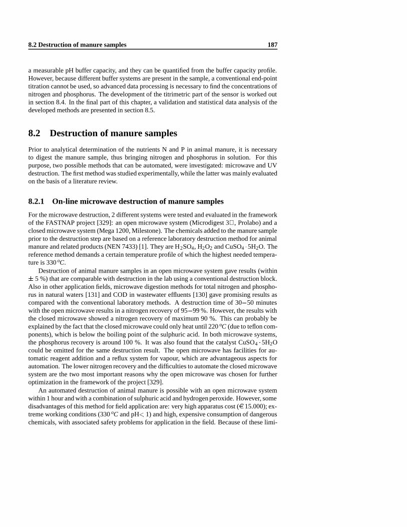
8.2 Destruction of manure samples 187
a measurable pH buffer capacity, and they can be quantified from the buffer capacity profile.However, because different buffer systems are present in the sample, a conventional end-pointtitration cannot be used, so advanced data processing is necessary to find the concentrations ofnitrogen and phosphorus. The development of the titrimetric part of the sensor is worked outin section 8.4. In the final part of this chapter, a validation and statistical data analysis of thedeveloped methods are presented in section 8.5.
8.2 Destruction of manure samples
Prior to analytical determination of the nutrients N and P in animal manure, it is necessaryto digest the manure sample, thus bringing nitrogen and phosphorus in solution. For thispurpose, two possible methods that can be automated, were investigated: microwave and UVdestruction. The first method was studied experimentally, while the latter was mainly evaluatedon the basis of a literature review.
8.2.1 On-line microwave destruction of manure samples
For the microwave destruction, 2 different systems were tested and evaluated in the frameworkof the FASTNAP project [329]: an open microwave system (Microdigest 3 , Prolabo) and aclosed microwave system (Mega 1200, Milestone). The chemicals added to the manure sampleprior to the destruction step are based on a reference laboratory destruction method for animalmanure and related products (NEN 7433) [1]. They are H2SO4, H2O2 and CuSO4 �5H2O. Thereference method demands a certain temperature profile of which the highest needed tempera-ture is 330 oC.
Destruction of animal manure samples in an open microwave system gave results (within� 5 %) that are comparable with destruction in the lab using a conventional destruction block.Also in other application fields, microwave digestion methods for total nitrogen and phospho-rus in natural waters [131] and COD in wastewater effluents [130] gave promising results ascompared with the conventional laboratory methods. A destruction time of 30�50 minuteswith the open microwave results in a nitrogen recovery of 95�99 %. However, the results withthe closed microwave showed a nitrogen recovery of maximum 90 %. This can probably beexplained by the fact that the closed microwave could only heat until 220 oC (due to teflon com-ponents), which is below the boiling point of the sulphuric acid. In both microwave systems,the phosphorus recovery is around 100 %. It was also found that the catalyst CuSO4 � 5H2Ocould be omitted for the same destruction result. The open microwave has facilities for au-tomatic reagent addition and a reflux system for vapour, which are advantageous aspects forautomation. The lower nitrogen recovery and the difficulties to automate the closed microwavesystem are the two most important reasons why the open microwave was chosen for furtheroptimization in the framework of the project [329].
An automated destruction of animal manure is possible with an open microwave systemwithin 1 hour and with a combination of sulphuric acid and hydrogen peroxide. However, somedisadvantages of this method for field application are: very high apparatus cost (e 15.000); ex-treme working conditions (330 oC and pH< 1) and high, expensive consumption of dangerouschemicals, with associated safety problems for application in the field. Because of these limi-

188 Automatic titrimetric sensor for manure nutrients
tations, an alternative destruction method based on UV-light was investigated for the purposeof manure destruction.
8.2.2 On-line UV destruction of manure samples
Literature overview of UV photodegradation applications UV destruction of organic ma-terial is applied for many different purposes: disinfection of water or wastewater [3, 154, 303],destruction of recalcitrant chemical substances (often aromatic structures) [52, 134, 245], mea-surement of nitrogen, phosphorus, : : : in water or soil solutions by photochemical decompo-sition [16, 113], etc. Photo-oxidation can enhance the biodegradability of wastewaters dueto removal of toxic pollutants [106, 153, 224], however a possible consequence of ultravioletphoto-oxidation can also be the induction of biotoxicity (e.g. algicidal effect) in treated waters[95, 252].
UV lamps can be classified by their radiation spectrum. This spectrum can be very nar-row, e.g. a monochromatic radiation at 254 nm, realized with a low-pressure mercury vapourlamp [29], or the spectrum can be very broad, e.g. a strong emission over the entire regionbetween 190 and 400 nm, realized with a high-pressure mercury vapour lamp [227]. Oxida-tion of chemicals by the UV process using low and medium pressure mercury vapour lampshinges on the generation of hydroxyl radicals [227]. Hydrogen peroxide (H2O2) is often usedin combination with low or medium pressure lamps, because the quantum yield of hydroxylradicals from hydrogen peroxide is almost 1 when the wavelength of UV light approaches 254nm. Applications based on this type of process are manyfold: UV/H2O2 treatment of indus-trial wastewater [117, 134, 194] or groundwater [152]. Sometimes the UV/H2O2 process isaccelerated by adding Fe2+ [245, 345] or ferrioxalate [245]. It is also possible to use H2O2 incombination with a catalyst (iron, graphite, activated carbon) without UV for the degradationof e.g. phenolic compounds [170]. For groundwater contaminated with volatile organic com-pounds (VOC’s), the Ultrox process (UV/H2O2/ozon) achieved VOC removals greater than 90% [152]. The oxidation of organic material with a combined persulphate/UV treatment is acommon technique used in TOC analyzers [42, 45]. A high-pressure mercury vapour lamp iseffective not only at generating hydroxyl radicals from H2O2 but also causing electronic tran-sitions in many organic molecules. Thus, this type of lamp is potentially capable of degradingorganics without the presence of a hydroxyl radical source [178, 227].
Titanium dioxide powder in aqueous solution is a well-known photocatalyst for the degra-dation of organics with solar or near-UV irradiation [27, 106, 142, 153, 195, 225]. A typicalconcentration for chemicals that can be mineralized with such treatment is around 1 mmol l�1,in a time period of 1�3 hours [184]. Full mineralization is not always possible, e.g. photocat-alytic degradation of atrazine [224]. The possible use of solar-illuminated TiO2 for the disin-fection of water is suggested [183]. By photocatalytic degradation with TiO2, dissolved organicnitrogens (DON’s) in natural waters are converted to inorganic nitrogens such as ammonium,nitrate and nitrite [276]. Other photocatalysts include magnetite and aluminium oxide [52],dyes like riboflavin [5, 333] and methylene blue [4, 5, 53], or naturally occurring substanceslike proteins [116]. Experiments with magnetite and a high-pressure mercury lamp [52] haveshown that it is possible to reduce the COD of a shale dry distillation wastewater from 2500ppmCOD to 1500 ppmCOD in 1 hour illumination time.
Photochemical decomposition of organic and inorganic phosphorus compounds into ortho-

8.2 Destruction of manure samples 189
phosphate has been developed for the determination of total phosphorus in natural and sewagewater [100, 209, 324, 348]. These methods rely on a combined strong acid (e.g. sulphuric acid)and strong UV treatment (e.g. 1000 W high pressure mercury lamp). This method is typicallyused in a range from 1�5000 µgP l�1. The determination of total nitrogen in water using on-line UV digestion is a possible alternative for the Kjeldahl method, especially for wastewatersamples with high nitrate content [145]. In this method, the organic and inorganic nitrogen isconverted into nitrate by potassium peroxodisulphate. In some cases (e.g. in the presence ofH2O2), nitrate acts like a filter and reduces the UV light intensity in the photoreactor [267].Without the addition of photocatalysts, it was found that organic nitrogen compounds are firstoxidized almost completely to nitrate which is then slowly reduced to nitrite on further irradi-ation [17].
Potential use of UV for manure destruction Based on the literature review presented aboveand some preliminary experiments, a comparative evaluation between UV and microwave de-struction of animal manure samples was made. The advantages of UV compared to microwavedigestion are:
� UV treatment can be done with cheaper equipment (e 3.000 for an UV reactor comparedto e 15.000 for a microwave oven).
� The technical construction of an UV photoreactor is more suited for automation com-pared to a microwave oven.
The disadvantages of UV compared to microwave digestion are:
� Organic nitrogen compounds are transformed into nitrate/nitrite with photo-oxidation.An oxidizing reagent (e.g. hydrogen peroxide or persulphate) is needed to transform allnitrogen containing organics (e.g. ureum) into nitrate/nitrite. It is uncertain if ammo-nium is also transformed into nitrate/nitrite.
� Organic phosphorus compounds are transformed into ortho-phosphate. However, ex-tra addition of oxidizing reagent is necessary to transform all phosphorus (includingpolyphosphates) into ortho-phosphate. Further, preliminary experiments showed thateven without UV treatment, almost 100 % recovery of phosphorus compounds from an-imal manure was realized when only sulphuric acid was added to the sample (personalcommunication, N. Walraven).
� Particulate materials are decreasing the efficiency of UV destruction due to light scat-tering. Therefore, perfect homogenization of the manure sample prior to destruction isnecessary. Also, the nutrient concentrations in animal manure are very high comparedto wastewaters and natural waters, so that a high dilution factor is required for the UVtreatment. However, this will consequently result in a lower accuracy of the N and Pmeasurements, due to the high heterogeneity of (even homogenized) animal manure.
Based on these points, it can be concluded that UV destruction is not a very strong alterna-tive for microwave digestion in the framework of this project. Especially if titrimetry is used ina further stage as measurement technique for nitrogen and phosphorus (see section 8.4), nitro-gen should be in the ammonium form for accurate quantification from a buffer capacity profile.Further, some preliminary experiments with a low pressure UV system were not very promis-ing, because of a low nitrogen recovery (personal communication, N. Walraven). Experiments

190 Automatic titrimetric sensor for manure nutrients
with a high pressure UV system could not be performed until now. In the framework of theFASTNAP project, further developments and optimizations were only based on the microwavedigestion.
8.3 Automatic nitrogen and phosphorus measurements
Before deciding on titration as the most adequate measurement technique for the automaticmanure sensor in the FASTNAP project, an exploratory study has been done to determinepotential techniques for automatic nitrogen and phosphorus determinations in manure [330,341]. In this study, the following techniques were evaluated:
� inductively coupled plasma - atomic emission spectroscopy (ICP-AES),� X-ray fluorescence (XRF),� near infrared spectroscopy (NIR), and� titrimetry.
All techniques show both advantages and disadvantages. Test measurements with an ICP-AES indicated that the phosphorus content in manure could be determined accurately [341].However, an ICP-AES is not capable of quantifying nitrogen [341]. In addition, it is a massivedevice and it is labour-intensive to operate. Further, samples must be digested before analysis.With XRF it is also impossible to quantify nitrogen. However, it should be able to measurephosphorus without sample pretreatment. NIR and titrimetry are non-proven technologies withrespect to the determination of nitrogen and phosphorus in manure. NIR has the advantage thatit is non-destructive and does not require digestion. There are examples in which nitrogen andphosphorus content in forage, food and beverage is determined with NIR [330]. Titrimetry wassuccessfully used for the determination of phosphate and ammonia in effluents, river waters andalgal treatment systems (see chapters 6 and 7). However, a disadvantage of titrimetry is thatmanure samples must be digested. The measuring time with NIR is much shorter than withtitrimetry (minutes compared to 1 hour). This puts NIR in favour of titrimetry with respect tospeed.
Based on:
� the possibility to analyze both nitrogen and phosphorus in a short amount of time, and� the successful analytical results in related research fields,
it is concluded that NIR and titrimetry are promising techniques for automatic measurementof nitrogen and phosphorus in manure samples [327, 330]. Because of the positive experi-ences with the pH buffer capacity based measurement method (see chapters 6 and 7), the lattertechnique was chosen for the further developments, which are presented in the next sections.
8.4 Development of the titrimetric part of the sensor
In this section, the different stages in the development of the titrimetric method for manuresamples are presented. First, the destruction method and its relation with the titration procedureis highlighted in sections 8.4.1, 8.4.2 and 8.4.3. A detailed simulation study with comparisons
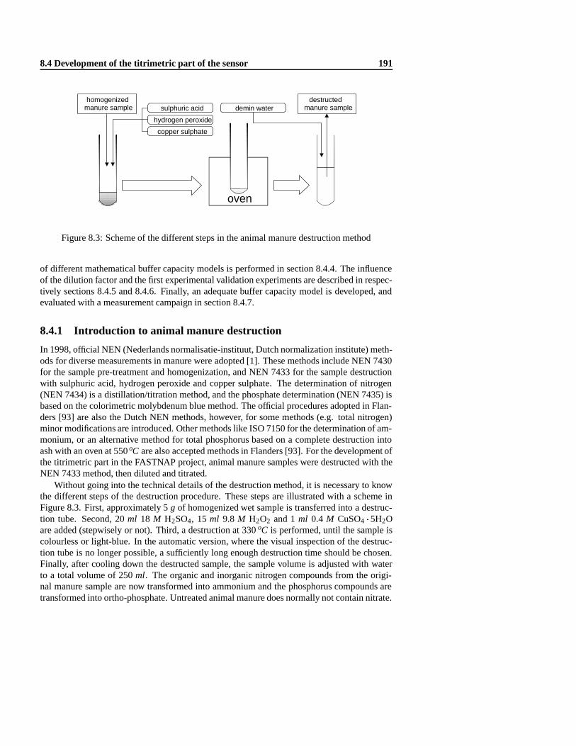
8.4 Development of the titrimetric part of the sensor 191
homogenized manure sample
destructed manure sample
oven
hydrogen peroxide
sulphuric acid
copper sulphate
demin water
Figure 8.3: Scheme of the different steps in the animal manure destruction method
of different mathematical buffer capacity models is performed in section 8.4.4. The influenceof the dilution factor and the first experimental validation experiments are described in respec-tively sections 8.4.5 and 8.4.6. Finally, an adequate buffer capacity model is developed, andevaluated with a measurement campaign in section 8.4.7.
8.4.1 Introduction to animal manure destruction
In 1998, official NEN (Nederlands normalisatie-instituut, Dutch normalization institute) meth-ods for diverse measurements in manure were adopted [1]. These methods include NEN 7430for the sample pre-treatment and homogenization, and NEN 7433 for the sample destructionwith sulphuric acid, hydrogen peroxide and copper sulphate. The determination of nitrogen(NEN 7434) is a distillation/titration method, and the phosphate determination (NEN 7435) isbased on the colorimetric molybdenum blue method. The official procedures adopted in Flan-ders [93] are also the Dutch NEN methods, however, for some methods (e.g. total nitrogen)minor modifications are introduced. Other methods like ISO 7150 for the determination of am-monium, or an alternative method for total phosphorus based on a complete destruction intoash with an oven at 550 oC are also accepted methods in Flanders [93]. For the development ofthe titrimetric part in the FASTNAP project, animal manure samples were destructed with theNEN 7433 method, then diluted and titrated.
Without going into the technical details of the destruction method, it is necessary to knowthe different steps of the destruction procedure. These steps are illustrated with a scheme inFigure 8.3. First, approximately 5 g of homogenized wet sample is transferred into a destruc-tion tube. Second, 20 ml 18 M H2SO4, 15 ml 9.8 M H2O2 and 1 ml 0.4 M CuSO4 � 5H2Oare added (stepwisely or not). Third, a destruction at 330 oC is performed, until the sample iscolourless or light-blue. In the automatic version, where the visual inspection of the destruc-tion tube is no longer possible, a sufficiently long enough destruction time should be chosen.Finally, after cooling down the destructed sample, the sample volume is adjusted with waterto a total volume of 250 ml. The organic and inorganic nitrogen compounds from the origi-nal manure sample are now transformed into ammonium and the phosphorus compounds aretransformed into ortho-phosphate. Untreated animal manure does normally not contain nitrate.

192 Automatic titrimetric sensor for manure nutrients
0
0.1
0.2
0.3
0.4
0.5
0.6
0.7
0.8
4 5 6 7 8 9 10
Buf
fer
capa
city
(m
eq l-1
pH
-1)
pH
measuredsimulated
Figure 8.4: Calculated buffer capacity points and corresponding simulation curve of a destruc-ted and 10 times diluted manure sample
However, if nitrate is present due to extra additions or treatments (e.g. aeration), a modifieddestruction method should be adopted [1, 173]. The concentrations of the added chemicals(except for H2O2 which is completely disintegrated) in the final destructed sample can be cal-culated and are 1.5 M sulphuric acid and 0.0016 M copper sulphate.
8.4.2 Titration of destructed manure samples
Experimental versus simulated buffer capacities In a first preliminary experiment, titra-tion curves of a destructed and 10 times diluted sample were recorded and interpreted. Amathematical model was used to simulate the buffer capacity curves. Prior to titration, the di-luted sample was adjusted to a pH 3 with NaOH 10 N. Figure 8.4 shows the calculated buffercapacity points from a recorded titration profile and the corresponding simulated buffer capac-ity profile. The simulation model contained: a water buffer, an IC buffer (to take into accountthe IC present in the titrant, or the headspace CO2 that eventually enters the sample duringtitration), an ortho-phosphate buffer, an ammonium buffer and a buffer around pH 3.7. A firstcomparison between laboratory and simulated concentrations is shown in Table 8.1. Figure 8.4illustrates that the simulated buffer capacity does not follow the experimental points around pH6. When additional buffers were added to the model, a better fit could not be obtained (resultsnot shown). This points to a possible phenomenon (e.g. precipitation) that is not included inthe simulation model. Further, from Table 8.1 it can be concluded that the phosphate in thetitrated sample was not found back as ortho-phosphate with the simulation model. Also, thesimulated concentration for IC is four times more than expected from calculations and previousexperiments. The extra buffer at pH 3.7 could not be explained at this stage.
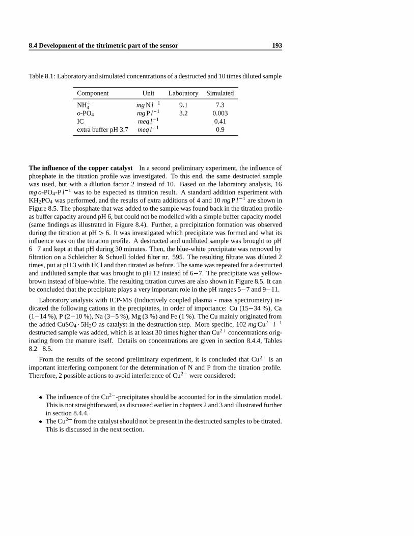
8.4 Development of the titrimetric part of the sensor 193
Table 8.1: Laboratory and simulated concentrations of a destructed and 10 times diluted sample
Component Unit Laboratory Simulated
NH+4 mgN l�1 9.1 7.3
o-PO4 mgP l�1 3.2 0.003IC meq l�1 0.41extra buffer pH 3.7 meq l�1 0.9
The influence of the copper catalyst In a second preliminary experiment, the influence ofphosphate in the titration profile was investigated. To this end, the same destructed samplewas used, but with a dilution factor 2 instead of 10. Based on the laboratory analysis, 16mg o-PO4-P l�1 was to be expected as titration result. A standard addition experiment withKH2PO4 was performed, and the results of extra additions of 4 and 10 mgP l �1 are shown inFigure 8.5. The phosphate that was added to the sample was found back in the titration profileas buffer capacity around pH 6, but could not be modelled with a simple buffer capacity model(same findings as illustrated in Figure 8.4). Further, a precipitation formation was observedduring the titration at pH > 6. It was investigated which precipitate was formed and what itsinfluence was on the titration profile. A destructed and undiluted sample was brought to pH6�7 and kept at that pH during 30 minutes. Then, the blue-white precipitate was removed byfiltration on a Schleicher & Schuell folded filter nr. 595. The resulting filtrate was diluted 2times, put at pH 3 with HCl and then titrated as before. The same was repeated for a destructedand undiluted sample that was brought to pH 12 instead of 6�7. The precipitate was yellow-brown instead of blue-white. The resulting titration curves are also shown in Figure 8.5. It canbe concluded that the precipitate plays a very important role in the pH ranges 5�7 and 9�11.
Laboratory analysis with ICP-MS (Inductively coupled plasma - mass spectrometry) in-dicated the following cations in the precipitates, in order of importance: Cu (15�34 %), Ca(1�14 %), P (2�10 %), Na (3�5 %), Mg (3 %) and Fe (1 %). The Cu mainly originated fromthe added CuSO4 � 5H2O as catalyst in the destruction step. More specific, 102 mgCu2+ l�1
destructed sample was added, which is at least 30 times higher than Cu2+ concentrations orig-inating from the manure itself. Details on concentrations are given in section 8.4.4, Tables8.2�8.5.
From the results of the second preliminary experiment, it is concluded that Cu2+ is animportant interfering component for the determination of N and P from the titration profile.Therefore, 2 possible actions to avoid interference of Cu2+ were considered:
� The influence of the Cu2+-precipitates should be accounted for in the simulation model.This is not straightforward, as discussed earlier in chapters 2 and 3 and illustrated furtherin section 8.4.4.
� The Cu2+ from the catalyst should not be present in the destructed samples to be titrated.This is discussed in the next section.

194 Automatic titrimetric sensor for manure nutrients
0
0.5
1
1.5
2
2.5
3
4 5 6 7 8 9 10
Buf
fer
capa
city
(m
eq l-1
pH
-1)
pH
sample as suchsample + 4 mg P l-1
sample + 10 mg P l-1filtrate obtained at pH 6
filtrate obtained at pH 12
Figure 8.5: Experimental buffer capacity curves of a destructed and 2 times diluted manuresample. Titration of the sample as such, the sample with standard additions of o-PO4, andfiltrates obtained at pH 6 and pH 12
8.4.3 Modification of the destruction procedure
A separate study by the Dutch partners in the FASTNAP project showed that the catalystCuSO4 �5H2O (NEN 7433) is not really necessary to obtain complete destruction. There wereno significant differences between laboratory measurements of nitrogen and phosphorus indestructed samples obtained with or without the catalyst. Therefore, it was decided to sim-plify the destruction procedure and perform all further destructions in the framework of theFASTNAP project without the copper catalyst (modified NEN 7433).
The consequences for the titrimetric measurement of the destructed manure samples with-out Cu2+ addition were twofold. First, precipitation during titration was not observed anymore (results not shown), and second, the sharp peak in the buffer capacity around pH 6 wasno longer present. When experimental buffer capacity curves were modelled with the samemodel as presented in section 8.4.2, a good fit between the experimental and simulated buffercapacity curves was obtained, but still differences between laboratory and titrimetric results inthe order of magnitude 20 % for ammonium and 100 % for phosphate were found (results notshown). Therefore, a more detailed study of the factors influencing the titrimetric nitrogen andphosphorus determination was performed, and is presented in the following sections.

8.4 Development of the titrimetric part of the sensor 195
Table 8.2: The composition of pig manure, based on 379 samples [118]
Component Unit Mean Minimum Maximum
Nitrogen mgN l�1 130 50 212Phosphorus mgP l�1 17 1 52Potassium mgK l�1 56 20 90Calcium mgCa l�1 50 7 217Magnesium mgMg l�1 18 2 36Chlorine mgCl l�1 34 12 88Sodium mgNa l�1 7 ND a 24Sulfur mgS l�1 13 ND a 25Boron mgB l�1 0.088 ND a 0.17Cadmium mgCd l�1 0.0006 ND a 0.0036Copper mgCu l�1 1.0 ND a 2.4Zinc mgZn l�1 1.0 ND a 3.5a ND: not detectable
8.4.4 Mathematical model analysis
Composition of destructed manure samples
To study which chemical phenomena influence the recorded titration curves, an insight in thecomplete composition of the destructed manure samples is necessary. With this information,and using mathematical models, a simulation study can be used to assess which reactions haveto be considered when modelling buffer capacity profiles. It should be mentioned that the mainpurpose of the buffer capacity modelling is to estimate the ammonium and ortho-phosphateconcentrations in the destructed manure samples.
A Dutch study [118] about animal manure composition was used to tabulate the mean, min-imum and maximum concentrations of measured components in animal manure. The originalresults are expressed as mg kg�1 manure, but for the purpose of this work, all values are ex-pressed as mgl�1 destructed and undiluted manure. Tables 8.2, 8.3 and 8.4 show the results forrespectively pigs, poultry and cattle. 1 Note that the concentration of sulfur originating fromthe H2SO4 added prior to the destruction step, is not included in the tables. This concentrationin the destructed samples is 1.5 M H2SO4.
A second study considered 19 different manure samples, originating from 2 mixed (pigsand cattle) farms in Flanders, taken in May 1998. The samples were analyzed for the sameelements as in the first study [118] (except for chlorine and sulfur), but supplemented with50 extra, mainly minor elements, all measured, except for nitrogen, with ICP-MS. Only thecomponents with a mean concentration higher than 0.1 mg l�1 and Cd are listed in Table 8.5.
1To convert values from l�1 destructed sample to kg�1 manure, the tabulated values should be multiplied with 50.
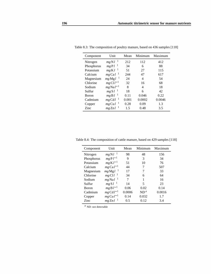
196 Automatic titrimetric sensor for manure nutrients
Table 8.3: The composition of poultry manure, based on 436 samples [118]
Component Unit Mean Minimum Maximum
Nitrogen mgN l�1 212 112 412Phosphorus mgP l�1 34 6 88Potassium mgK l�1 51 27 115Calcium mgCa l�1 244 47 617Magnesium mgMg l�1 24 4 54Chlorine mgCl l�1 32 16 68Sodium mgNa l�1 8 4 18Sulfur mgS l�1 18 6 42Boron mgB l�1 0.11 0.046 0.22Cadmium mgCd l�1 0.001 0.0002 0.0046Copper mgCu l�1 0.28 0.09 1.3Zinc mgZn l�1 1.5 0.48 3.5
Table 8.4: The composition of cattle manure, based on 429 samples [118]
Component Unit Mean Minimum Maximum
Nitrogen mgN l�1 98 48 156Phosphorus mgP l�1 9 3 34Potassium mgK l�1 51 10 76Calcium mgCa l�1 44 7 507Magnesium mgMg l�1 17 7 33Chlorine mgCl l�1 34 6 64Sodium mgNa l�1 7 1 16Sulfur mgS l�1 14 5 23Boron mgB l�1 0.06 0.02 0.14Cadmium mgCd l�1 0.0006 ND a 0.0016Copper mgCu l�1 0.14 0.032 1.7Zinc mgZn l�1 0.5 0.12 3.4a ND: not detectable

8.4 Development of the titrimetric part of the sensor 197
Table 8.5: The composition of 19 manure samples from Flemish pigs and cattle
Component Unit Mean Minimum Maximum
Nitrogen mgN l�1 128 53 241Phosphorus mgP l�1 40 4 102Potassium mgK l�1 94 42 137Calcium mgCa l�1 52 7 152Magnesium mgMg l�1 29 1 63Sodium mgNa l�1 16 3 32Boron mgB l�1 0.13 0.06 0.26Cadmium mgCd l�1 0.001 0.0003 0.002Copper mgCu l�1 0.75 0.06 4.3Zinc mgZn l�1 5 0.21 38Aluminum mgAl l�1 3 0.07 10Titanium mgTi l�1 0.11 0.004 0.3Manganese mgMn l�1 0.8 0.03 1.7Iron mgFe l�1 7 0.7 22Strontium mgSr l�1 0.14 0.02 0.4Barium mgBa l�1 0.13 ND a 0.8a ND: not detectable

198 Automatic titrimetric sensor for manure nutrients
Table 8.6: Ionic strength calculations in destructed manure samples for different dilution fac-tors and the corresponding corrections for pKa and γH+ to be included in buffer capacity models
Dilution factor
undiluted 2 times 6.6 times 10 times
SO2�4 (M) 1.5 0.75 0.227 0.15
Na+ (M) 3 1.5 0.454 0.3I (M) 4.5 2.25 0.68 0.45∆pKa H3PO4=H2PO�
4 �0:12 �0:13∆pKa H2PO�
4 =HPO2�4 �0:37 �0:4
∆pKa HPO2�4 =PO3�
4 �0:62 �0:67∆pKa H2CO�
3=HCO�3 �0:12 �0:13
∆pKa HCO�3 =CO2�
3 �0:37 �0:4∆pKa NH+
4 =NH3 +0:12 +0:13∆pKa H2O=OH� �0:12 �0:13∆pKa HSO�
4 =SO2�4 �0:37 �0:4
γH+ 0.75 0.74
Ionic strength influence
The ionic strength of the destructed manure mainly originates from the quantity of H2SO4
added to the manure prior to the destruction step, and the quantity of strong NaOH added tothe destructed sample to bring it to pH 3, prior to the titration. All other ionic substances(e.g. NH+
4 , HPO2�4 , Ca2+) are mostly far below 15 mmol l�1, before as well as during the
titration. These quantities are negligible compared to the quantities of SO2�4 and Na+ which
are respectively 1.5 and 3 M in the destructed and undiluted manure sample.Table 8.6 reports the ionic strength in function of different dilution factors. The ionic
strength is calculated with the formula for I given in Table 2.1 on page 16. Next, the activitycoefficients γ were calculated for a number of ions that need to be considered in the mathe-matical models for buffer capacity. However, only the Davies approximation (see Table 2.1on page 16) is useful, because its applicability reaches an ionic strength upper level of 0.5M. Next, the necessary calculations were done to correct the mathematical models for theinfluence of ionic strength (see section 3.3.6 on page 51 and section 3.5.4 on page 63). Thesymbol ∆pKa is used for the difference between the pK0
a (taking into account the effect of ionicstrength) and the pKa (assuming no influence of ionic strength). A ∆pKa value can be positiveor negative, depending on the considered buffer system. The ∆pKa values for some importantbuffer systems in the destructed samples, and the activity coefficient of H+ are also given in Ta-ble 8.6. Note that the latter calculations are only performed for the two highest dilution factors,because for the lower dilution factors, the ionic strength is too high for reliable calculations,even with the Davies approximation. The dilution factor 6.6 is included because this factor wasexperimentally found as the optimal dilution factor (see section 8.4.5). Therefore, the further

8.4 Development of the titrimetric part of the sensor 199
0
0.5
1
1.5
2
2.5
4 5 6 7 8 9 10 11
Buf
fer
capa
city
(m
eq l-1
pH
-1)
pH
without activity correctionwith activity correction
Figure 8.6: Simulated buffer capacity curves of a destructed and 6.6 times diluted manuresample, with and without ionic strength correction in the model
simulation examples in this section are performed with this particular dilution factor.The effect of the ionic strength correction is illustrated in Figure 8.6. The buffer capacity
curve of a destructed and 6.6 times diluted manure sample with mean concentrations for am-monium and ortho-phosphate, was simulated. A small amount of inorganic carbon (IC) (0.11mmol l�1) was also included in the model. The simulation was performed with and withoutthe ionic strength correction. No complexation or precipitation reactions were included in thismodel. It can be concluded that the ionic strength correction has a significant effect on thebuffer capacity profile, and should be considered in the mathematical models.
Complexation and precipitation
Based on the complete analysis of 19 manure samples (see Table 8.5), it was investigatedwhich complexation and precipitation reactions might have an influence on the buffer capacityprofile in the pH range between pH 3 and pH 11. This is a difficult task, in the first placebecause of the caveats related to precipitation and dissolution reactions, formulated in section2.5 on page 35. Experimental findings have shown that buffer capacity curves are not veryreproducible when precipitation reactions are involved. Further, in section 3.5.5 on page 64, itwas discussed that in systems where different possible solids involving common componentsexist, it is not straightforward to obtain the correct set of solids to be included in the math-ematical model. These aspects make the modelling of precipitation phenomena difficult andunwieldy. Complexation reactions (see section 2.4 on page 29) are equilibrium reactions thatfrom a kinetic point of view are in most cases fast or very fast. They are easy to incorporatein mathematical models for buffer capacity (e.g. with the tableau-method discussed in section

200 Automatic titrimetric sensor for manure nutrients
Table 8.7: Concentrations of different components included in the buffer capacity model withthe purpose to evaluate precipitation and complexation reactions
Component Concentration
SO2�4 0.227 mol l�1
NH+4 2.6 mmol l�1
o-PO4 0.5 mmol l�1
Ca2+ 0.58 mmol l�1
Fe3+ 0.06 mmol l�1
3.5 on page 55). However, the difficulty is that there are possibly hundreds of complexationreactions that can be considered in destructed manure. Based on the composition of destruc-ted manure (see Table 8.5), the metal cations known as complex formers are Ca2+, Mg2+,Fe3+, Al3+, Zn2+ and Cu2+. Rare complex formers, but present in high concentrations are K+
and Na+. Possible ligands in destructed manure are H2O, OH�, SO2�4 , NH3, PO3�
4 , HPO2�4 ,
H2PO�4 . During titration, some CO2 can enter in the titration vessel, thus at high pH, also
CO2�3 can be considered as a possible ligand.
With preliminary simulation tests, using the software bctab(see section 5.2 on page 113),a number of complexation and precipitation reactions were investigated for their effect on thebuffer capacity profile. With the above mentioned cations and ligands, hundreds of possiblecomplexation or precipitation reactions must be considered. Therefore, more detailed simula-tion studies were restricted to a choice of 2 cations, Ca2+ and Fe3+, that are present in ratherhigh concentrations, and that are considered to have an important influence on the buffer ca-pacity profile between pH 4 and pH 11. It was also chosen not to include carbonate equilibriaat this stage. The concentrations of the different components included in the buffer capacitymodel, for the purpose of complexation and precipitation modelling, are tabulated in Table 8.7.The concentrations are chosen as the maximum values from Table 8.5, and take into account a6.6 times dilution.
First, a number of simple chemical equilibrium reactions were considered in the mathemat-ical model, given in Table 8.8. The logK values are given at 25 oC [273], and the logK 0 values(mixed acidity constants, see section 2.2.4 on page 19) were calculated to account for ionicactivities in the model. Contrary to preliminary simulation experiments (see section 8.4.2), thesulphuric acid buffer was now included in the model. Despite the fact that H2SO4 is a strongacid, its influence on the buffer capacity is considered significant due to its high concentrationin the destructed manure. Second, also complexation reactions were included in the model.Table 8.9 summarizes the complex formation reactions and corresponding logβ values (logβvalues were taken from [273] at 25 oC). Because some reactions involve the binding of morethan 1 ligand anion, overall formation constants (symbols β and β0) and not stepwise forma-tion constants (symbol K) were used (see also section 2.4.1 on page 30). Third, a numberof precipitation reactions were investigated with the bctabsoftware. They are summarized inTable 8.10 (logKs0 were taken from [263, 273] at 25 oC). The concentration product log cKs0

8.4 Development of the titrimetric part of the sensor 201
Table 8.8: Simple chemical equilibrium reactions included in the mathematical model
Chemical reaction logK logK0
H++H2PO�4 H3PO4 2.15 2.03
H++HPO2�4 H2PO�
4 7.2 6.83H++PO3�
4 HPO2�4 12.35 11.73
H++NH3 NH+4 9.24 9.36
H++SO2�4 HSO�
4 1.99 1.62H++OH�
H2O 14 13.88
Table 8.9: Complex chemical equilibrium reactions included in the mathematical model
Chemical reaction logβ logβ0
Ca2++H2PO�4 CaH2PO+
4 1.45 0.96Ca2++HPO2�
4 CaHPO04 2.75 1.76
Ca2++PO3�4 CaPO�
4 6.5 5.01Ca2++OH�
CaOH+ 1.15 0.66Ca2++SO2�
4 CaSO04 2.31 1.32
Fe3++H2PO�4 FeH2PO2+
4 4.35 3.61Fe3++HPO2�
4 FeHPO+4 10.15 8.66
Fe3++OH� FeOH2+ 11.8 11.1
Fe3++2OH� Fe(OH)+2 22.3 21.07
Fe3++4OH� Fe(OH)�4 34.4 32.9
Fe3++SO2�4 FeSO+
4 4.0 2.51Fe3++2SO2�
4 Fe(SO4)�2 5.4 3.42
(introduced in equation (2.74) on page 36) is used for the ionic activity corrected logKs0 value,where concentrations instead of activities can be used.
Note that hydroxy-apatite (Ca5(PO4)3OH(s)) is a precipitate that is typically found in ani-mal manure. However, this reaction proceeds very slowly to an equilibrium, i.e. the solutioncan highly, and for a long time, be supersaturated before any precipitation starts (unless thereare already crystal seeds present in the solution) [263].
In a first stage, the simulation study only considered the simple and the complex chemicalequilibria. In a later phase, the precipitation reactions were evaluated. The chemical reactionsin Tables 8.8 and 8.9 need to be organized into a stoichiometric matrix and a correspondinginput file for the program bctab. This process is described and illustrated with an examplein section 3.5.3 on page 61. The species, components and stoichiometric information, repre-senting the reactions presented in Tables 8.8 and 8.9, is organized in a tableau in Table 8.11.

202 Automatic titrimetric sensor for manure nutrients
Table 8.10: Precipitation and dissolution reactions included in the mathematical model
Chemical reaction logKs0 log cKs0
Ca2++HPO2�4 CaHPO4(s) �6:65 �5:66
Ca2++2H2PO�4 Ca(H2PO4)2(s) �1:14 �0:40
Ca2++2OH� Ca(OH)2(s) �5:19 �4:45
Ca2++SO2�4 CaSO4(s) �4:62 �3:63
Fe3++PO3�4 FePO4(s) �(21:9�26:4) �(19:7�24:2)
Fe3++3OH� Fe(OH)3(s) �(38:8�42:7) �(37:3�41:2)
5Ca2++3PO3�4 +OH�
Ca5(PO4)3OH(s) �55:9 �50:0
The simulation results of 2 models, with and without the complex formation reactions, areshown in Figure 8.7. There are 3 regions in the buffer capacity profile that are influenced bythe complex formation reactions from Table 8.9. They are indicated with arrows on the graph.Extra simulations, where complex formation reactions were evaluated separately or in smallergroups, revealed the responsible reactions for the buffer capacity increases. Region (1), aroundpH 5.5, is related to iron and phosphate; region (2), around pH 8, is related to iron hydroxides;and region (3), around pH 10, is originating from calcium and phosphate. It should be notedthat, in the simulation study, the maximum concentrations of Ca2+ and Fe3+ found in a setof manure samples (see Table 8.5) were used. Thus, in real situations, the influences of thecomplex formation reactions are probably lower than illustrated in Figure 8.7.
The final purpose of the buffer capacity modelling in this application is to make an es-timation of the ortho-phosphate and ammonium concentrations in the destructed and dilutedmanure samples. Therefore, an interesting conclusion from this simulation study is that thebuffer capacities around pH 6.7 and pH 9�9.5 are influenced only to a minor extent by thecomplex formation reactions. As a consequence, a reliable estimation of ortho-phosphate andammonium is still possible, even if the exact concentrations of calcium and iron are unknown.
In a second stage, the simulation study evaluated the precipitation reactions in Table 8.10on their occurrence between pH 2 and pH 11 during the simulation of the model shown in Table8.11. The program bctabhas a built-in facility to calculate the ionic concentration product of2 or more species that can form a possible precipitate at each pH value. This concentrationproduct is then compared with the log cKs0 value, to find the state of saturation of the solutionwith respect to that solid. If the solution is oversaturated, a message for that solid is loggedin a file. The precipitates that are theoretically formed and their corresponding pH ranges, aretabulated in Table 8.12. Three possible precipitates were found under the modelled conditions.As mentioned before, the precipitation of hydroxy-apatite is most uncertain, and will not befurther considered. An interesting point is that there are no calcium precipitates formed, butonly two iron precipitates. The precipitate that is theoretically formed at first during a pHincrease is iron hydroxide. The consequences for the simulated buffer capacity profile whenFe(OH)3(s) precipitation is considered, are presented in the following paragraphs.

8.4 Development of the titrimetric part of the sensor 203
Table 8.11: Species, components and stoichiometric information for simple and complexchemical equilibrium reactions in destructed and diluted manure
Components
Species H3PO4 NH+4 HSO�
4 Ca2+ Fe3+ H+ flogKgH3PO4 1 0 0 0 0 0 0NH+
4 0 1 0 0 0 0 0HSO�
4 0 0 1 0 0 0 0Ca2+ 0 0 0 1 0 0 0Fe3+ 0 0 0 0 1 0 0H2PO�
4 1 0 0 0 0 �1 �2:03HPO2�
4 1 0 0 0 0 �2 �8:86PO3�
4 1 0 0 0 0 �3 �20:6NH3 0 1 0 0 0 �1 �9:36SO2�
4 0 0 1 0 0 �1 �1:62CaH2PO+
4 1 0 0 1 0 �1 �1:08CaHPO0
4 1 0 0 1 0 �2 �7:1CaPO�
4 1 0 0 1 0 �3 �15:6CaOH� 0 0 0 1 0 �1 �13:23CaSO0
4 0 0 1 1 0 �1 �0:3FeH2PO2+
4 1 0 0 0 1 �1 1.58FeHPO+
4 1 0 0 0 1 �2 �0:2FeOH2+ 0 0 0 0 1 �1 �2:82Fe(OH)+2 0 0 0 0 1 �2 �6:69Fe(OH)�4 0 0 0 0 1 �4 �22:6FeSO+
4 0 0 1 0 1 �1 0.89Fe(SO4)
�2 0 0 2 0 1 �2 0.18
OH� 0 0 0 0 0 �1 �13:88
C (mol l�1) 0.0005 0.0026 0.227 0.00058 6 10�5
Table 8.12: Theoretical precipitations found with the simulation model for destructed anddiluted manure between pH 2 and pH 11
Precipitate Precipitation in pH interval
FePO4(s) 3.35�8.45Fe(OH)3(s) 2.75�11Ca5(PO4)3OH(s) 7.35�11

204 Automatic titrimetric sensor for manure nutrients
0
0.5
1
1.5
2
4 5 6 7 8 9 10 11
Buf
fer
capa
city
(m
eq l-1
pH
-1)
pH
(1)
(2)
(3)without complex formations
with complex formations
Figure 8.7: Simulated buffer capacity curves of a destructed and diluted manure sample, withand without complex formation reactions in the model. Three arrows indicate a buffer capacityincrease due to the complex formation reactions
When considering precipitation reactions, the stoichiometric information has to be rewrit-ten in function of the precipitates that are considered. An example that illustrates how a pre-cipitation reaction has to be included in the stoichiometric information is given in section 3.5.5on page 64. It is mentioned there, that if more than one precipitation reaction needs to be con-sidered, a trial and error procedure may be necessary to find the correct stoichiometric matrix.And further, for each simulation pH step, the stoichiometric matrix should be reconsideredfor its validity, because the set of precipitates can change along increasing pH values. This isunwieldy for practical purposes, and therefore, it is advised to consider only a minimal numberof precipitates (1 or 2 precipitates) for buffer capacity simulation purposes. Also, as describedin section 2.5 on page 35, precipitation reactions are sluggish, slow, non-stoichiometric, : : :Thus, mathematical modelling results of such reactions during a relatively ‘ fast’ titration pro-cess (from pH 3 to pH 11 in around 30 minutes), should be interpreted with carefulness.
The Fe(OH)3(s) is considered as a type IV solid (see section 3.5.2 on page 60) in thisexample. Its presence decreases the number of degrees of freedom for solving this equilibriumproblem. More particularly, the concentration of free iron [Fe3+] is directly linked to the pHby the following reaction:
[Fe3+][OH�]3 = 10�40 or log[Fe3+] = 1:64+3log[H+] (8.1)
Thus, the stoichiometric information in Table 8.11 needs to be adjusted when Fe(OH)3(s) isinvolved. Fe3+ is not considered any more as a component, and species including Fe3+ needto be rewritten using equation (8.1). The new stoichiometric matrix is presented in Table 8.13.
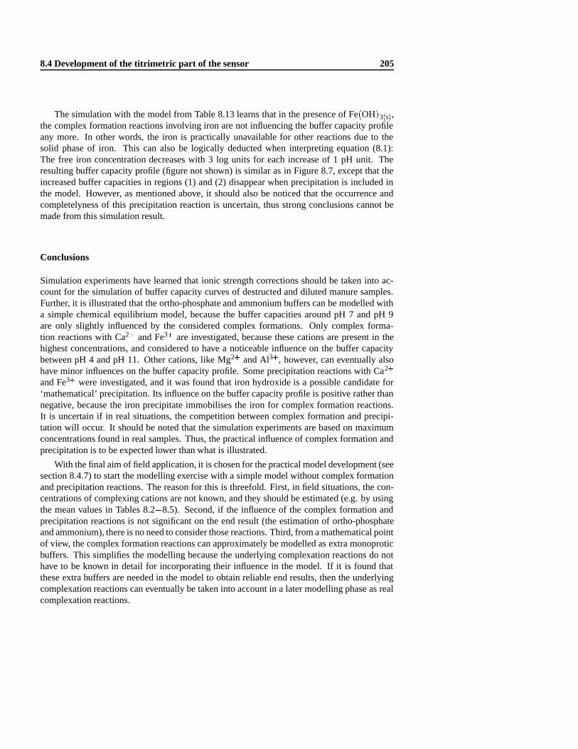
8.4 Development of the titrimetric part of the sensor 205
The simulation with the model from Table 8.13 learns that in the presence of Fe(OH)3(s),the complex formation reactions involving iron are not influencing the buffer capacity profileany more. In other words, the iron is practically unavailable for other reactions due to thesolid phase of iron. This can also be logically deducted when interpreting equation (8.1):The free iron concentration decreases with 3 log units for each increase of 1 pH unit. Theresulting buffer capacity profile (figure not shown) is similar as in Figure 8.7, except that theincreased buffer capacities in regions (1) and (2) disappear when precipitation is included inthe model. However, as mentioned above, it should also be noticed that the occurrence andcompletelyness of this precipitation reaction is uncertain, thus strong conclusions cannot bemade from this simulation result.
Conclusions
Simulation experiments have learned that ionic strength corrections should be taken into ac-count for the simulation of buffer capacity curves of destructed and diluted manure samples.Further, it is illustrated that the ortho-phosphate and ammonium buffers can be modelled witha simple chemical equilibrium model, because the buffer capacities around pH 7 and pH 9are only slightly influenced by the considered complex formations. Only complex forma-tion reactions with Ca2+ and Fe3+ are investigated, because these cations are present in thehighest concentrations, and considered to have a noticeable influence on the buffer capacitybetween pH 4 and pH 11. Other cations, like Mg2+ and Al3+, however, can eventually alsohave minor influences on the buffer capacity profile. Some precipitation reactions with Ca2+
and Fe3+ were investigated, and it was found that iron hydroxide is a possible candidate for‘mathematical’ precipitation. Its influence on the buffer capacity profile is positive rather thannegative, because the iron precipitate immobilises the iron for complex formation reactions.It is uncertain if in real situations, the competition between complex formation and precipi-tation will occur. It should be noted that the simulation experiments are based on maximumconcentrations found in real samples. Thus, the practical influence of complex formation andprecipitation is to be expected lower than what is illustrated.
With the final aim of field application, it is chosen for the practical model development (seesection 8.4.7) to start the modelling exercise with a simple model without complex formationand precipitation reactions. The reason for this is threefold. First, in field situations, the con-centrations of complexing cations are not known, and they should be estimated (e.g. by usingthe mean values in Tables 8.2�8.5). Second, if the influence of the complex formation andprecipitation reactions is not significant on the end result (the estimation of ortho-phosphateand ammonium), there is no need to consider those reactions. Third, from a mathematical pointof view, the complex formation reactions can approximately be modelled as extra monoproticbuffers. This simplifies the modelling because the underlying complexation reactions do nothave to be known in detail for incorporating their influence in the model. If it is found thatthese extra buffers are needed in the model to obtain reliable end results, then the underlyingcomplexation reactions can eventually be taken into account in a later modelling phase as realcomplexation reactions.

206 Automatic titrimetric sensor for manure nutrients
Table 8.13: Species, components and stoichiometric information for simple and complexchemical equilibrium reactions in destructed and diluted manure, in the presence of iron hy-droxide precipitate. The bold items mark the differences with Table 8.11
Components
Species H3PO4 NH+4 HSO�
4 Ca2+ H+ flogKgH3PO4 1 0 0 0 0 0NH+
4 0 1 0 0 0 0HSO�
4 0 0 1 0 0 0Ca2+ 0 0 0 1 0 0Fe3+ 0 0 0 0 3 1.64H2PO�
4 1 0 0 0 �1 �2:03HPO2�
4 1 0 0 0 �2 �8:86PO3�
4 1 0 0 0 �3 �20:6NH3 0 1 0 0 �1 �9:36SO2�
4 0 0 1 0 �1 �1:62CaH2PO+
4 1 0 0 1 �1 �1:08CaHPO0
4 1 0 0 1 �2 �7:1CaPO�
4 1 0 0 1 �3 �15:6CaOH� 0 0 0 1 �1 �13:23CaSO0
4 0 0 1 1 �1 �0:3FeH2PO2+
4 1 0 0 0 2 3.22FeHPO+
4 1 0 0 0 1 1.44FeOH2+ 0 0 0 0 2 �1.18Fe(OH)+2 0 0 0 0 1 �5.05Fe(OH)�4 0 0 0 0 �1 �20.96FeSO+
4 0 0 1 0 2 2.53Fe(SO4)
�2 0 0 2 0 1 1.82
OH� 0 0 0 0 �1 �13:88
C (mol l�1) 0.0005 0.0026 0.227 0.00058

8.4 Development of the titrimetric part of the sensor 207
Table 8.14: Titrimetric nitrogen and phosphorus determination in destructed manure for dif-ferent dilution factors. The concentrations are expressed as mg l�1 in the undiluted destructedsample
NH+4 (mgN l�1) o-PO4 (mgP l�1)
Dilution factor Mean Std. dev. Mean Std. dev.
Undiluted 208 4.6 77 4.92 � 202 3.6 71 2.73 � 197 5.6 74 4.46 � 191 6.3 74 4.415� 182 14.2 77 13.2
Laboratory 171 76
8.4.5 The influence of the dilution factor
Destructed manure samples contain 1:5 M H2SO4, and have an extremely low pH value. Priorto titration, the pH needs to be adjusted with a strong alkaline solution (e.g. NaOH 1.5 N) tobring the pH around 3. Next, a titration with NaOH 0.1 N is performed until pH 11 is reached.If destructed manure samples are titrated without dilution, a number of problems can arise.First, the alkaline consumption, NaOH 1.5 and 0.1 N in this case, would be very high. Second,the ionic strength would be very high and its effect on the activities of ions cannot be predictedany more by approximate formulas (see Table 8.6). Third, unwanted chemical reactions, likeprecipitation, can interfere with the buffer capacity measurement. On the other hand, whendestructed samples are diluted too much, the concentrations of phosphate and ammonium inthe solution become too low, and the effect of measurement noise and interferences of e.g. in-organic carbon become too large. Consequently, the variability and accuracy of the final resultwould be negatively influenced. An experiment was set up to test different dilution factors andevaluate their effects on the estimates of ortho-phosphate and ammonium concentrations.
A destructed manure sample was used to prepare 5 different dilutions, ranging from undi-luted to 15 times diluted. Each diluted series was titrated in fourfold. The laboratory analy-ses of the nitrogen and phosphorus concentrations of that sample were 171 mgN l �1 and 76mgP l�1. The ammonium and the ortho-phosphate concentrations were also estimated from theexperimental buffer capacity curves, and the results are tabulated in Table 8.14. Two examplesof experimental and corresponding simulated buffer capacity curves for respectively undilutedand 15 times diluted sample are shown in Figure 8.8.
For the undiluted samples, the experimental buffer capacity curves became irregular for pHvalues higher than 9, as illustrated in Figure 8.8(a). This can possibly be explained by slowreactions like precipitation reactions. This was also observed in the 2 times diluted sample, butno longer for the higher dilutions. Despite the irregular buffer capacity curves for the undilutedand two times diluted sample, the estimates for N and P are still reproducible, as can be seen inthe rather low standard deviations on the N and P estimates in Table 8.14. The simulated buffer

208 Automatic titrimetric sensor for manure nutrients
0
1
2
3
4
5
6
7
8
9
10
11
5 6 7 8 9 10 11
Buf
fer
capa
city
(m
eq l-1
pH
-1)
pH
(a)
measuredsimulated
0
0.2
0.4
0.6
0.8
1
1.2
1.4
1.6
1.8
5 6 7 8 9 10 11
Buf
fer
capa
city
(m
eq l-1
pH
-1)
pH
(b)
measuredsimulated
Figure 8.8: Experimental and simulated buffer capacity curves of destructed manure. Plot (a)undiluted sample. Plot (b) 15 � diluted sample. Note the difference in scale
capacity curves for the highest dilution factor (see Figure 8.8(b)) fit much better in the high pHrange, compared to the fit of the undiluted samples. However, the standard deviations obtainedthrough the 4 replicate concentration values, become too high for the highest dilution factorcompared to the lower dilution factors (see Table 8.14). The dilution factors 3 and 6 gavethe best results, because unwanted precipitations or other reactions were avoided, and stillreproducible results were obtained. Because of the corresponding lowest chemical demands,factor 6 was chosen as the ideal dilution factor for further experiments.
8.4.6 Experimental method validation
A number of experiments were set up to experimentally study some anticipated phenomenathat were already investigated with simulations in section 8.4.4. In a first stage, the influenceof sulphuric acid, ionic strength and Ca2+ were investigated. In a second stage, a standardaddition experiment with o-PO4 was performed to validate the followed approach.
Without going into the details of the the first stage experiments (full results in [300]), thereare some important conclusions to be made from these experiments. Despite the fact that sul-phuric acid is a strong acid, its influence on the buffer capacity in destructed and diluted manuresamples (e.g. 0.23 M in 6.6 times diluted sample) is clearly felt up to pH 6.5. Therefore, theHSO�
4 H++SO2�4 reaction needs to be incorporated in the buffer capacity model. Addi-
tion experiments with NaCl (up to 0.3 M) to change the ionic strength of titrated samples haveillustrated that the ∆pKa’s predicted by the Davies approximation fairly well correspond withthe observations in the buffer capacity profiles (see also Table 8.6). Addition experiments withCaCl2 (up to 150 mgCa2+ l�1) have shown that the Ca2+ did not have a significant effect onthe buffer capacity profile of destructed and diluted manure. This confirms that a simple math-ematical model (without complexation and precipitation) may be sufficient for the modellingof the buffer capacity curves of destructed manure samples.
In the second stage, a standard addition experiment with KH2PO4 on a destructed manuresample was performed. The concentrations in the sample were 117 mgN l�1 and 25 mgP l�1.

8.4 Development of the titrimetric part of the sensor 209
Table 8.15: Titrimetric nitrogen and phosphorus determination in destructed manure for dif-ferent standard additions of ortho-phosphate. The concentrations are expressed as mg l�1 indestructed and undiluted sample
Standard addition NH+4 (mgN l�1) o-PO4 (mgP l�1) o-PO4 recovery
(mgP l�1) Mean Std. dev. Mean Std. dev. (mgP l�1) (%)
0 118.9 0.57 23.2 0.614.76 119.2 0.22 27.6 0.50 4.37 929.52 119.0 0.26 31.6 0.21 8.35 8819.0 119.4 0.25 40.3 0.55 17.1 9028.6 119.4 0.55 49.2 0.31 26.0 9138.1 120.0 0.13 57.9 0.57 34.7 9147.6 120.5 0.63 67.1 0.58 43.9 92
The stock solution of KH2PO4 was tested on its concentration with a colorimetric method(Cuvette test LCK049, Dr. Lange ). Subsamples were prepared as follows: 25 ml from thedestructed manure sample was diluted with 100 ml water. Around 70 ml of NaOH 1 N wasadded manually to bring the pH of the sample to pH 3. Thus, the total sample volume wasaround 195 ml and therefore, the dilution factor was 7.8. The titrations were performed witha laboratory titrator (Metrohm Titrino 716) with the DET titration mode (details of the DETtitration algorithm can be found in section 5.1.1 on page 98). The normality of the titrant was0.1 N and the end pH value was 11. Around 10 ml of titrant was added during the titration. Thetemperature of the samples was the same as the room temperature during the experiment (24to 25 oC). Seven series of samples (blank and standard additions between 5 and 50 mgP l�1
destructed and undiluted sample, see Table 8.15) were titrated in fivefold. Contrary to theprevious and following experiments reported in this section, the NaOH stock solutions 1 Nand 0.1 N were not prepared in the laboratory with NaOH pellets and demineralized water, butwere bought as 10 litre, completely closed, plastic bags (Titripack , Merck). The reason forthis is described in detail in section 8.5.2.
The mathematical modelling of the experimental buffer capacity curves was performedin two steps. First, the ‘blank’ curves (without extra ortho-phosphate addition) were modelledand it was found that besides the ortho-phosphate and ammonium buffers, two additional smallbuffers around pH 5.1 and pH 8.4 were present. These 2 buffers were quantified as respectively0.060 and 0.095 mmol l�1 in the diluted samples. Second, another model was used, in whichthe 2 extra buffers were included as fixed buffer capacities. The second model was applied toother experimental buffer capacity curves and the amount of ortho-phosphate and ammoniumwas estimated.
The results of this standard addition experiment are given in Table 8.15. The ammoniumand ortho-phosphate concentrations estimated from the buffer capacity profiles showed a goodreproducibility, with a standard deviation around 0.5 mgl�1 for both N and P. The ammoniumconcentrations estimated from the buffer capacity profiles increased with increasing additions

210 Automatic titrimetric sensor for manure nutrients
of ortho-phosphate. This increase was small (< 2 mgN l�1), however, statistically significant(p< 0:001). The recovery of ortho-phosphate for the different standard additions was in allcases around 90 %. With a paired t-test, it was concluded that the recovered concentrations ofortho-phosphate were significantly different (p< 0:001) from the added concentrations. Thiscould point to possible other chemical reactions with ortho-phosphate, which are not includedin the model, e.g. complexation reactions. The small increases in the estimated ammoniumconcentration with increasing ortho-phosphate standard additions points to possible formationof ortho-phosphate complexes that are buffering around pH 9, and being modelled as ammo-nium instead of ortho-phosphate (see also arrow (3) in Figure 8.7).
8.4.7 Development of an adequate buffer capacity model
A measurement campaign was organized to evaluate different mathematical buffer capacitymodels. The estimated ammonium and ortho-phosphate concentrations from the buffer capac-ity profile were compared with the laboratory analyses. A most adequate model is formulated,that will be proposed for further validations and later field-use.
The manure samples were collected in May 1998 on two mixed farms (pigs and cattle) inFlanders. At very different places on both farms, 19 samples were taken. All samples weredestructed with the modified NEN 7433 method (see section 8.4.3) and analyzed in the lab forN and P. The destructed samples were titrated as follows: 25 ml of destructed sample wasdiluted with 100 ml water. Around 40 ml of NaOH 1.5 N was added manually to bring thepH of the sample to pH 3. Thus, the total sample volume was around 165 ml, correspondingwith a dilution factor 6.6. This dilution factor was chosen in correspondence with the resultsof section 8.4.5. Between the manual pH adjustment and the titration, the samples were stirredfor 20 minutes at pH 3 with a magnetic stirrer at high speed, to remove inorganic carbon(CO2) originating from the NaOH 1.5 N stock solution. The titrations were performed witha laboratory titrator (Metrohm Titrino 716) with the DET titration mode (details of the DETtitration algorithm can be found in section 5.1.1 on page 98). The normality of the titrant was0.1 N and the end pH value was 11. Around 10 ml of titrant was added during the titration.The temperature of the samples was the same as the room temperature (around 20 oC), but noextra temperature control was used during the titrations. All samples were diluted and titratedin threefold.
Two criteria were used to interpret the results obtained with different buffer capacity mod-els. First, the fit between the experimental and the simulated buffer capacity data was visu-alized and interpreted. Second, tables and scatterplots with the laboratory measurements ofnitrogen and phosphorus against the estimated concentrations from the titrimetric measure-ments were interpreted. Different mathematical models were fitted to the experimental data.The software bomb(see section 5.3 on page 117) was used for the buffer capacity calculationand modelling. An overview of the model specifications of 4 selected models is given in Table8.16. The results of 1 selected manure sample for the different models are tabulated in Ta-ble 8.17 and the corresponding experimental and simulated buffer capacity curves are shownFigure 8.9.
Model 1 is the initial model, containing the main buffer components to be expected in thedestructed and diluted manure samples. Ionic activity corrections as calculated theoretically insection 8.4.4 were applied to the zero ionic strength pKa values at 25 oC. All pKa values were

8.4 Development of the titrimetric part of the sensor 211
Table 8.16: Model specifications of 4 selected models used during the development of the mostadequate model for destructed and 6.6 times diluted manure samples. The concentrations areexpressed per volume of destructed and diluted sample. The bold items mark the differenceswith the previous model
Unit Model 1 Model 2 Model 3 Model 4
pKa H2O 15.62 15.62�15.82 15.62�15.82 15.62�15.82pKa1 IC 6.25 6.1 6.1 6.1pKa2 IC 9.88 9.85 9.85 9.85pKa1 o-PO4 2.0 1.9 1.9 1.9pKa2 o-PO4 6.84 6.7 6.7 6.7pKa3 o-PO4 12.05 11.9 11.9 11.9pKa SO2�
4 1.52 1.1 1.1 1.1
pKa NH+4 9.2�9.5 9.25�9.75 9.25�9.75 9.25�9.75
pKa blank1 4.5�5.5pKa blank2 7.5�8.4CIC mgCO2 l�1 0.75�2.2 0.75�2.2 0.75�2.2 0.75�2.2Co-PO4 mgP l�1 0�25 0�25 0�25 0�25CSO2�
4mol l�1 0.227 0.227 0.227 0.227
CNH+4
mgN l�1 0�45 0�45 0�45 0�45
Cblank1 mmol l�1 0�1Cblank2 mmol l�1 0�1
γH+ 0.75 0.75 0.75 0.75pH interval 5.6�10.5 5.6�10.5 4�10.5 5.6�10.5
Table 8.17: Simulation results of 1 selected sample for the 4 different models. The concentra-tions are expressed as mg l�1 or mmol l�1 in destructed and diluted sample
Unit Laboratory Model 1 Model 2 Model 3 Model 4
pKa H2O 15.72 15.72 15.72pKa NH+
4 9.5 9.74 9.74 9.75pKa blank1 5.18pKa blank2 7.88CIC mgCO2 l�1 1.08 2.2 0.75 2.15Co-PO4 mgP l�1 9.82 8.56 9.32 9.18 8.14CNH+
4mgN l�1 36.5 35.9 38.3 38.8 38.3
Cblank1 mmol l�1 0.12Cblank2 mmol l�1 0.063
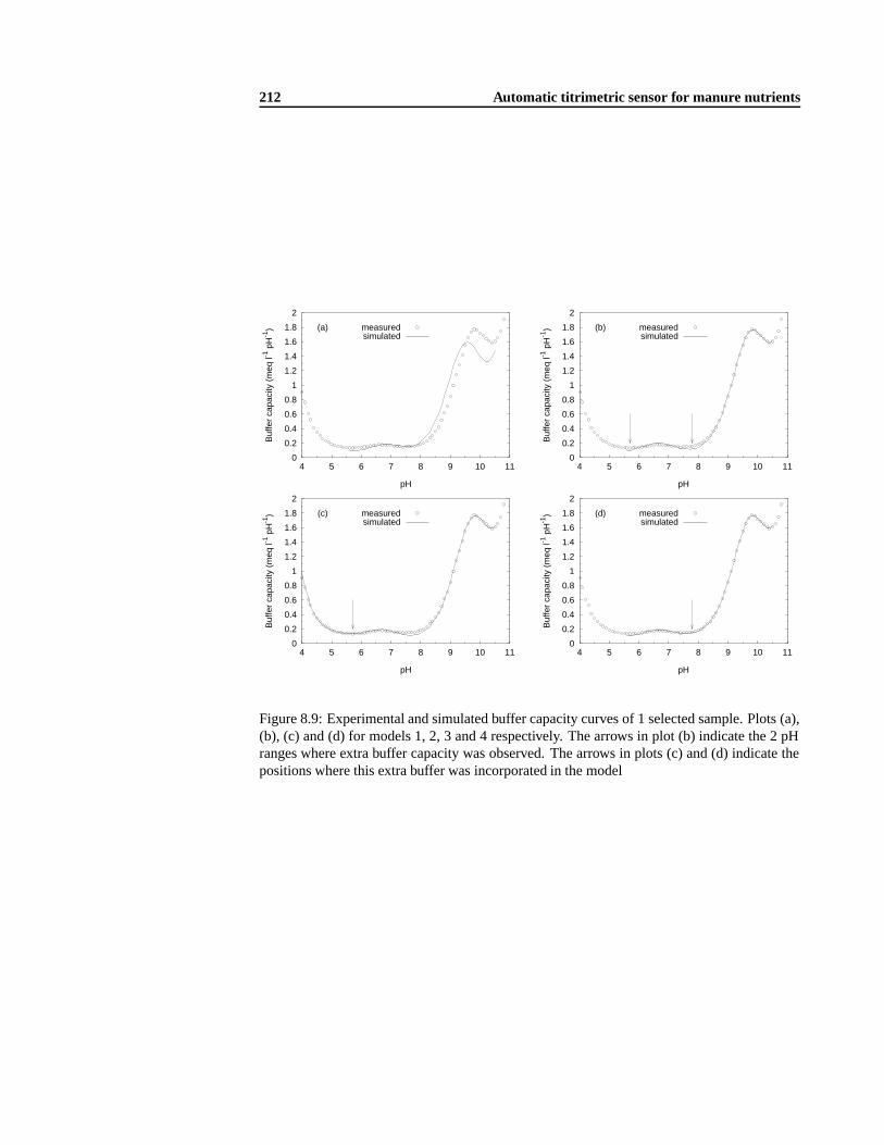
212 Automatic titrimetric sensor for manure nutrients
0
0.2
0.4
0.6
0.8
1
1.2
1.4
1.6
1.8
2
4 5 6 7 8 9 10 11
Buf
fer
capa
city
(m
eq l-1
pH
-1)
pH
(a) measuredsimulated
0
0.2
0.4
0.6
0.8
1
1.2
1.4
1.6
1.8
2
4 5 6 7 8 9 10 11
Buf
fer
capa
city
(m
eq l-1
pH
-1)
pH
(c) measuredsimulated
0
0.2
0.4
0.6
0.8
1
1.2
1.4
1.6
1.8
2
4 5 6 7 8 9 10 11
Buf
fer
capa
city
(m
eq l-1
pH
-1)
pH
(b) measuredsimulated
0
0.2
0.4
0.6
0.8
1
1.2
1.4
1.6
1.8
2
4 5 6 7 8 9 10 11
Buf
fer
capa
city
(m
eq l-1
pH
-1)
pH
(d) measuredsimulated
Figure 8.9: Experimental and simulated buffer capacity curves of 1 selected sample. Plots (a),(b), (c) and (d) for models 1, 2, 3 and 4 respectively. The arrows in plot (b) indicate the 2 pHranges where extra buffer capacity was observed. The arrows in plots (c) and (d) indicate thepositions where this extra buffer was incorporated in the model

8.4 Development of the titrimetric part of the sensor 213
kept fixed, except for the pKa of the ammonium buffer, which was allowed to vary between avalue 9.2 and 9.5. A fixed or variable pKa value for ammonium did not make much differencein the estimates of the concentrations, but a variable pKa for ammonium gave a better fitbetween the experimental and simulated buffer capacity profiles. When the pKa2 value forortho-phosphate allowed to vary, the estimations of phosphate became worse. Therefore, itwas chosen to set the pKa of ammonium as a parameter to be optimized and to keep the otherpKa’s fixed. It was experienced in chapters 6 and 7 that a small amount of inorganic carbon(IC) is found back in the buffer capacity profile. Initially, a variable amount of IC between 0and 5 mgCO2 l�1 was included in the buffer capacity model. Later, it was found, generally,that a more narrow range gives somewhat more realistic results, especially in the samples witha low phosphate concentration (< 10 mgP l�1). This can be explained by the fact that theIC buffer is located near the ortho-phosphate buffer in the buffer capacity profile, thus thosetwo buffers are more or less exchangeable with each other. Therefore, the amount of IC wasallowed to vary between 0.75 and 2.2 mgCO2 l�1 only. On the experimental buffer capacitycurves, it was noticed that some buffer capacity around pH 5 was present, which could notoriginate from the buffer components included in model 1. Because at this stage, this buffercapacity was not of interest, it was chosen to limit the pH range for the simulation from pH 5.6to pH 10.5. Generally spoken, the estimated concentrations of N and P obtained with model1 were acceptable. However, the experimental and simulated buffer capacity curves did not fitvery well. This is illustrated in Figure 8.9(a).
Model 2 is the result of manual adjustments of the ‘fi xed’ pKa values in the model, in orderto obtain a better fit and a more accurate prediction of the concentrations. The adjustmentsthat were made can be read from Table 8.16 when comparing model 1 with model 2. It canbe noticed that for all buffers (except for H2O), the adjustments of the fixed pKa values are inthe same direction as if the samples would have a higher ionic strength than the values usedfor a 6.6 times diluted sample in Table 8.6. More particular, all pKa values were decreaseda little bit, except for the NH+
4 and the H2O buffer, where the pKa’s were increased. It wasfound that the pKa of the H2O buffer influenced the quality of the NH+
4 prediction and the fitaround pH 10. The best value for the pKa of H2O was 15.69. However, because this pKa valuewas so determining for the estimated ammonium concentration, it was investigated if the resultwas still acceptable if the pKa of water was allowed to vary instead of being a fixed value. Theconclusion was that a variable pKa for water gives similar results as a fixed pKa. The advantageof a variable pKa is that biased pH measurements (e.g. due to calibration errors) and deviationsof the real pKa compared to the theoretical pKa (e.g. ionic interaction effects) can slightly be‘corrected’ in the model by allowing some extra flexibility on the considered pKa in the model.Therefore, for robustness reasons, a variable pKa was preferred. There are several explanationspossible why the theoretical pKa values did not correspond with the practical observations.There could be a calibration error or an alkaline error in the pH measurement (see section2.1.3 on page 10). Also, there can be an effect of the temperature, which was not kept at 25 oC.The pH meter did not have automatic temperature compensation, and internally kept the Nernstslope always as if the temperature of the solution was 25 oC. The theoretical pKa values thatwere used, were those tabulated at 25 oC. Finally, due to the high ionic strength in the samples(even at 6.6 times diluted), the formulas for the activity corrections (Davies approximationin this case) are at their limit of applicability. Therefore, the real ∆pKa’s can differ from thevalues calculated in Table 8.6.

214 Automatic titrimetric sensor for manure nutrients
Considering the results of the selected manure sample (see Table 8.17) and the other 18manure samples in the study (results not shown), model 2 was found to be better than model 1.The estimated concentrations CIC for the different samples varied between the minimum andmaximum boundary values (respectively 0.75 and 2.2 mgCO2 l�1). However, in around 50 %of the samples, the estimated IC concentration equalled the maximum boundary value (see alsothe example in Table 8.17). Increasing the boundary value resulted in a worse estimation ofortho-phosphate. This points to the important interfering property of IC for the quantificationof ortho-phosphate. In Figure 8.9(b), one notices that in the experimental data, some buffercapacity exists around pH 5 and pH 8 (indicated with arrows) which can not be modelledwith model 2, because no buffer systems around these pH ranges are included in the model.This phenomenon was noticed in most samples. Therefore, the two next models respectivelyincorporated an extra buffer in those two pH ranges.
Model 3 is an extension of model 2, with the incorporation of an extra monoprotic bufferin the model, whose pKa may vary between pH 4.5 and pH 5.5. The pKa and the concentrationof that buffer are estimated by fitting the model to the experimental data. The simulation pHinterval was extended, and set from pH 4 to pH 10.5. The typical result is a better fit in thepH range 4 to 7, as illustrated with the selected example in Figure 8.9(c). The estimations ofNH+
4 did not change in model 3 compared to model 2. However, the estimations of o-PO4
were slightly worse in model 3 compared to model 2. The extra buffer in model 3 was at most0.17 mmol l�1. There is a remarkable difference in the concentration of IC found with model2 compared to model 3 (see Table 8.17). In model 2, the estimated IC is at its upper limit(2.2 mgCO2 l�1), whereas in model 3, the estimated IC is at its lower limit (0.75 mgCO2 l�1).This suggests that the extra monoprotic buffer in model 3 is interfering to some extent withthe IC buffer. Also, in Figure 8.9(c), it can be noticed that around pH 8, there is some extraexperimental buffer capacity, not accounted for in the simulated buffer capacity profile.
Model 4 is an alternative extension of model 2, with an extra monoprotic buffer whosepKa may vary between pH 7.5 and pH 8.4. Again, the fit between the experimental and thesimulated data was better than in model 2, illustrated for the selected sample in Figure 8.9(d).The extra buffer in model 4 was at most 0.16 mmol l�1. The estimations of o-PO4 were sys-tematically underestimated and with a higher variability (not shown in Table 8.17) in model 4compared to model 2. Unfortunately, this extra buffering component is thus interfering withthe ortho-phosphate buffer estimations at pH 6.7.
To get more insight in the origin of the two extra buffers around pH 5 and pH 8, a correlationanalysis was performed between the data obtained with ICP-MS on those samples (see section8.4.4 and Table 8.5) and the concentrations of ‘blank1’ and ‘blank2’ obtained with models3 and 4 respectively. The Pearson correlation coefficients with their significance level aretabulated in Table 8.18. From these correlations, it can be concluded that Ca2+, Mg2+, N andP correlate best with ‘blank1’ at pH 5, and that Cu2+ and Zn2+ correlate best with ‘blank2’at pH 8. Fe3+ and Al3+ correlate very significant with both blank buffers. This is fairly wellin correspondence with the findings of the simulation study in section 8.4.4, more particularlywith what is illustrated in Figure 8.7. The ‘blank1’ and ‘blank2’ buffers exactly correspondwith the 2 regions in the buffer capacity profile influenced by complex formation reactionswith Ca2+ and Fe3+. In the simulation study, it was found that the buffer capacity in ‘blank1’was originating from iron and phosphate. In this correlation study, iron and phosphate are bothcorrelating very significant with ‘blank1’ . Further, the simulation study also revealed that the
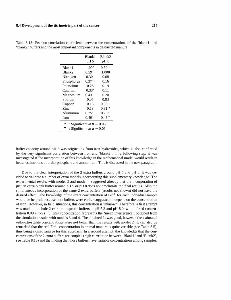
8.4 Development of the titrimetric part of the sensor 215
Table 8.18: Pearson correlation coefficients between the concentrations of the ‘blank1’ and‘blank2’ buffers and the most important components in destructed manure
Blank1 Blank2pH 5 pH 8
Blank1 1.000 0.59��
Blank2 0.59�� 1.000Nitrogen 0.30� 0.08Phosphorus 0.37�� 0.16Potassium 0.26 0.19Calcium 0.33� 0.11Magnesium 0.43�� 0.20Sodium 0.05 0.03Copper 0.18 0.53��
Zinc 0.18 0.61��
Aluminum 0.75�� 0.78��
Iron 0.40�� 0.45��
� : Significant at α = 0:05�� : Significant at α = 0:01
buffer capacity around pH 8 was originating from iron hydroxides, which is also confirmedby the very significant correlation between iron and ‘blank2’ . In a following step, it wasinvestigated if the incorporation of this knowledge in the mathematical model would result inbetter estimations of ortho-phosphate and ammonium. This is discussed in the next paragraph.
Due to the clear interpretation of the 2 extra buffers around pH 5 and pH 8, it was de-cided to validate a number of extra models incorporating this supplementary knowledge. Theexperimental results with model 3 and model 4 suggested already that the incorporation ofjust an extra blank buffer around pH 5 or pH 8 does not ameliorate the final results. Also thesimultaneous incorporation of the same 2 extra buffers (results not shown) did not have thedesired effect. The knowledge of the exact concentration of Fe3+ for each individual samplewould be helpful, because both buffers were earlier suggested to depend on the concentrationof iron. However, in field situations, this concentration is unknown. Therefore, a first attemptwas made to include 2 extra monoprotic buffers at pH 5.3 and pH 8.0, with a fixed concen-tration 0.08 mmol l�1. This concentration represents the ‘mean interference’ , obtained fromthe simulation results with models 3 and 4. The obtained fit was good, however, the estimatedortho-phosphate concentrations were not better than the results with model 2. It can also beremarked that the real Fe3+ concentration in animal manure is quite variable (see Table 8.5),thus being a disadvantage for this approach. In a second attempt, the knowledge that the con-centrations of the 2 extra buffers are coupled (high correlation between ‘Blank1’ and ‘Blank2’ ,see Table 8.18) and the finding that those buffers have variable concentrations among samples,

216 Automatic titrimetric sensor for manure nutrients
were implemented in a new model. The model contained again the 2 extra buffers at pH 5.3and pH 8.0, but with concentrations that were allowed to vary, however, with the restrictionthat both concentrations must be equal within 1 sample. The minimum boundary for the sim-ulation interval was also slightly modified from pH 5.6 to pH 5.3. The fit of this model wasexcellent, but the estimated ortho-phosphate concentrations were again systematically under-estimated. From all the studied models considering the extra buffers around pH 5 and/or pH 8,this model was found to perform the best when comparing the estimated concentrations withthe laboratory concentrations.
Besides the buffer capacity models described above, some more mathematical models wereevaluated. The other models that were studied contained the same buffer systems as describedin models 1 to 4. However, they contained different boundary values on the pKa values andconcentrations (e.g. CIC) that were allowed to vary. It was also investigated if the pKa’sof sulphate, IC and ortho-phosphate are best kept fixed or allowed to vary. Finally, model2 was found to be the most adequate model for further validations and possible field-use.A scatterplot of the laboratory analyses against the titrimetric estimations with model 2 forrespectively ammonium and ortho-phosphate are presented in Figure 8.10(a) and (b). Further,a relative error (%) was calculated to express the difference between the titrimetric and thelaboratory concentrations.
relative error (%) =Ctitrimetric�Claboratory
Claboratory�100 (8.2)
The corresponding graphs with the relative errors for ammonium and ortho-phosphate are pre-sented in Figure 8.10(c) and (d).
Figure 8.10(a) and (b) illustrates that the linearity between the 2 measurement techniquesis very good. However, the ammonium concentrations estimated from the buffer capacityprofile were in most cases overestimated compared to the corresponding laboratory measure-ments. For ortho-phosphate, only one, very low loaded sample (3.5 mgP l �1, measured inthe laboratory) was overestimated with more than 25 %. All other samples were within rel-ative differences between �2 % and +18 % for ammonium and between �15 % and +30 %for ortho-phosphate, as illustrated in Figure 8.10. Based on these results, a new experimentwas set up, to validate the ‘most adequate model’ with completely new manure samples. Thisvalidation experiment is described in the following section.
8.5 Laboratory validation and statistical data analysis
8.5.1 Validation experiment
A second measurement campaign was organized to validate the results and the most adequatemodel described in section 8.4.7. Fifty-three samples were collected in April 1999, at farmsrandomly selected in the Netherlands and Flanders. More particularly, several manure trans-portation companies have cooperated to collect samples at the most diverse places. Each sam-ple was homogenized, and two subsamples (duplo A and B) were taken. Each subsample wasdestructed and analyzed in the laboratory for N and P. All destructed samples were 6.6 timesdiluted and titrated in threefold, with the same procedures as described in section 8.4.7. In

8.5 Laboratory validation and statistical data analysis 217
0
50
100
150
200
250
300
0 50 100 150 200 250 300
Am
mon
ium
(m
g N
l-1, t
itrim
etric
)
Ammonium (mg N l-1, laboratory)
(a)
-20
-15
-10
-5
0
5
10
15
20
0 50 100 150 200 250 300
Rel
ativ
e er
ror
(%)
Ammonium (mg N l-1, laboratory)
(c)
0
10
20
30
40
50
60
70
80
0 10 20 30 40 50 60 70 80
Ort
ho-p
hosp
hate
(m
g P
l-1, t
itrim
etric
)
Ortho-phosphate (mg P l-1, laboratory)
(b)
-50
-25
0
25
50
75
100
125
150
175
200
0 10 20 30 40 50 60 70 80
Rel
ativ
e er
ror
(%)
Ortho-phosphate (mg P l-1, laboratory)
(d)
Figure 8.10: Laboratory and titrimetric analyses of ammonium (a) and ortho-phosphate (b)with the corresponding relative error of the titrimetric analyses of ammonium (c) and ortho-phosphate (d) for 19 different manure samples and using the most adequate buffer capacitymodel. The concentrations are expressed as mg l�1 destructed and undiluted sample

218 Automatic titrimetric sensor for manure nutrients
total, 318 titration curves (53 samples, 2 subsamples and 3 replicates) were recorded, in a pe-riod of 14 days. The sequence of those 318 titrations was split in 12 blocks, of which 1 blockcontained 27 different manure samples of 1 subsample (duplo A or B) and 1 replicate. Eachblock corresponded with one measurement day. With such experimental design, eventual un-controllable effects (e.g. of temperature, electrode, titrant, : : : ) could be determined with ananalysis of variance, including a block effect. The temperature in the laboratory was around22 oC, and fairly well constant due to the isolated location of the laboratory. No extra measureswere taken to keep the temperature as constant as possible, and the minimum and maximumtemperature recorded in the lab during the complete experiment was respectively 20 and 24 oC.
During this experiment, the stock solutions of NaOH 0.1 N and 1.5 N had to be preparedseveral times (6 times 1 litre for the stock of NaOH 0.1 N and at least 10 times 1 litre forthe stock of NaOH 1.5 N). These stocks were prepared with pro analyse NaOH pellets, andthe exact titre was determined with oxalic acid dihydrate ((COOH)2 � 2H2O) titrations. Thepro analyse pellets were taken from two different pots (an almost empty one and a new one)that were in use in the lab at that moment. The stock solutions were stored in dark brownglass bottles, equipped with a bowed CO2 absorption tube. Contrary to the first measurementcampaign (see section 8.4.7), the majority of destructed samples were brought to pH 3 withthe automatic titrator. Only a few samples were manually brought to pH 3, for which an olderNaOH 1.5 N stock that was standing in the lab, was used. The above rather detailed descriptionof stock solution origin, storage, etc. is necessary to introduce a prior unnoticed problem ofinterferences in the buffer capacity profiles. It was found that for almost 50 % of the samples,the reproducibility of the 3 replicates (recorded at different days, with different stock solutions)was worse than in previous experiments. The problems were related to the stock solutions, andare described and investigated in section 8.5.2. For this reason, a number of titration curveswere eliminated for further data analysis. A total of 253 titration curves were considered asacceptable and were further processed with the software bomb.
A number of mathematical models were fitted to the experimental buffer capacity curvesof this data set, and comparisons between laboratory and titrimetric measurements were made.The same methodology as applied in section 8.4.7 was used here, i.e. first trying with a simple,basic model, then extending the model with extra buffers, while at the same time also eval-uating the pKa values, i.e. whether they are best kept fixed or allowed to vary, etc. It wasconcluded that the most adequate model found in section 8.4.7 also applied as such for thenew data set. This points to the robustness of this model in different situations. A scatterplotof the laboratory analyses against the titrimetric estimations with the most adequate model forrespectively ammonium and ortho-phosphate are presented in Figure 8.11(a) and (b). The cor-responding graphs with the relative errors for ammonium and ortho-phosphate are presentedin Figure 8.11(c) and (d).
The titrimetric ammonium estimations are all lying between �7 % and +8 % relative er-ror compared to the laboratory measurements. This result is even better than what was foundin the first measurement campaign, used for the model development. The results of the titri-metric ortho-phosphate estimation are similar as in the previous experiment. For the sampleswith a laboratory ortho-phosphate concentration higher than 10 mgP l �1, a relative error be-tween �15 % and +45 % was found. However, the relative errors of the samples with a lowlaboratory ortho-phosphate concentration are unexpectedly high. More particularly, the titri-metric concentrations are systematically higher than the laboratory concentrations. The origin

8.5 Laboratory validation and statistical data analysis 219
0
50
100
150
200
250
300
0 50 100 150 200 250 300
Am
mon
ium
(m
g N
l-1, t
itrim
etric
)
Ammonium (mg N l-1, laboratory)
(a)
-20
-15
-10
-5
0
5
10
15
20
0 50 100 150 200 250 300
Rel
ativ
e er
ror
(%)
Ammonium (mg N l-1, laboratory)
(c)
0
10
20
30
40
50
60
70
80
0 10 20 30 40 50 60 70 80
Ort
ho-p
hosp
hate
(m
g P
l-1, t
itrim
etric
)
Ortho-phosphate (mg P l-1, laboratory)
(b)
-50
-25
0
25
50
75
100
125
150
175
200
0 10 20 30 40 50 60 70 80
Rel
ativ
e er
ror
(%)
Ortho-phosphate (mg P l-1, laboratory)
(d)
Figure 8.11: Laboratory and titrimetric analyses of ammonium (a) and ortho-phosphate (b)with the corresponding relative error of the titrimetric analyses of ammonium (c) and ortho-phosphate (d) using the buffer capacity model developed in section 8.4.7 (53 different manuresamples). The concentrations are expressed as mg l�1 destructed and undiluted sample

220 Automatic titrimetric sensor for manure nutrients
of these rather bad results was pointed out to be interferences originating from the NaOH stocksolutions. These are described and further investigated in section 8.5.2.
From the samples with a laboratory ortho-phosphate concentration lower than 10 mgP l �1
(12 samples from the 53), duplo A and B were titrated again. New NaOH stock solutions 0.1and 1.5 N with pellets from an almost new pot NaOH ‘pro analyse’ , were prepared at the sameday of the titrations. The other experimental conditions were the same as before. The samemathematical model was used, with one small modification. In the original model, the min-imum and maximum boundaries for the amount of inorganic carbon were respectively set to0.75 and 2.2 mgCO2 l�1. For the newly recorded titration curves, the amount of inorganic car-bon was found to be more constant than before, around 1.6 mgCO2 l�1. Therefore, the rangefor the concentration of CO2 in the model, was set between 1.3 and 1.8 mgCO2 l�1. A simi-lar scatterplot with the laboratory analyses against the titrimetric estimations for respectivelyammonium and ortho-phosphate are presented in Figure 8.12(a) and (b). The correspondinggraphs with the relative errors for ammonium and ortho-phosphate are presented in Figure8.12(c) and(d).
On the one hand, the differences between the titrimetric and laboratory ammonium con-centrations are in a similar range as noticed in the first data set of the validation experiment(compare Figure 8.12(a) and (c) with respectively Figure 8.11(a) and (c)). However, there isa tendency that in the samples containing less phosphorus, the estimations of ammonium aresystematically around 5 % lower than the corresponding laboratory values. On the other hand,a very significant increase in accuracy was reached for the titrimetric ortho-phosphate esti-mation (compare Figure 8.12(b) and (d) with respectively Figure 8.11(b) and (d) in the rangebetween 0 and 10 mgP l�1). The relative errors on P of the 12 repeated low-loaded samplesare now in the same order as the relative errors of the high-loaded samples.
A first conclusion that can be drawn from this validation experiment is that the estimatedconcentrations for N and P with the titrimetric method are in a practical useful and acceptablerange compared to the official laboratory methods. However, a more detailed statistical anal-ysis of the variability and measurement errors is necessary to formulate a more statisticallysupported conclusion. This statistical analysis is described in section 8.5.3. A second conclu-sion resulting from this validation experiment is that important interferences are originatingfrom the NaOH stock solutions. Especially in the low loaded samples, the ‘quality’ of thestock solutions is of major importance for the accuracy of the P estimations. The interferencesoriginating from the NaOH are presented and discussed in section 8.5.2.
8.5.2 Influences of alkaline stock solutions
During the validation experiment described in section 8.5.1, it was found that the reproducibil-ity of the buffer capacity profiles of several destructed and diluted manure samples, titratedwith different NaOH stock solutions, was poor. When putting all the measurement results to-gether, it was quickly recognized that the poor reproducibility was originating from the NaOHstock solutions, and not from temperature effects, calibration errors, etc. A detailed descrip-tion on how the alkaline stock solutions were prepared and stored was already given in section8.5.1.
A series of new experiments were set up, to investigate and define the origin of the poorreproducibility. A pool of 6 different destructed manure samples was made, to be able to

8.5 Laboratory validation and statistical data analysis 221
0
50
100
150
0 50 100 150
Am
mon
ium
(m
g N
l-1, t
itrim
etric
)
Ammonium (mg N l-1, laboratory)
(a)
-20
-15
-10
-5
0
5
10
15
20
0 50 100 150
Rel
ativ
e er
ror
(%)
Ammonium (mg N l-1, laboratory)
(c)
0
1
2
3
4
5
6
7
8
9
10
0 1 2 3 4 5 6 7 8 9 10
Ort
ho-p
hosp
hate
(m
g P
l-1, t
itrim
etric
)
Ortho-phosphate (mg P l-1, laboratory)
(b)
-50
-25
0
25
50
75
100
125
150
175
200
0 1 2 3 4 5 6 7 8 9 10
Rel
ativ
e er
ror
(%)
Ortho-phosphate (mg P l-1, laboratory)
(d)
Figure 8.12: Laboratory and titrimetric analyses of ammonium (a) and ortho-phosphate (b)with the corresponding relative error of the titrimetric analyses of ammonium (c) and ortho-phosphate (d) using the buffer capacity model developed in section 8.4.7 (12 repeated manuresamples). The concentrations are expressed as mg l�1 destructed and undiluted sample

222 Automatic titrimetric sensor for manure nutrients
titrate the same sample under varying conditions. The sample preparations and titrations wereperformed as described in section 8.4.7. In short, a destructed and diluted manure sample wasfirst set to pH 3 with around 40 ml of a 1.5 N NaOH stock solution. Next, the sample wasstirred for 20 minutes to remove CO2 originating from the alkaline stock solution. Last, thesample was titrated to pH 11 with around 10 ml of a 0.1 N NaOH stock solution.
The following 4 stock solutions of NaOH were used in a first series of experiments:Stock 1.5(a) : Stock solution of 1.5 N, prepared in the laboratory at the day of the measure-
ments, with pellets from a new pot ‘NaOH pro analyse’ . The solution was keptin a dark brown glass bottle, equipped with a CO2 scrubber (bowed glass tubewith soda lime pellets).
Stock 1.5(b) : Two months old stock solution of 1.5 N, kept in a closed dark brown glassbottle, but without a CO2 scrubber. This solution was earlier used for manualpH adjustments of destructed manure samples. When not in use, the bottlewas kept closed. It is noteworthy that during this period of 2 months, a brownprecipitate was formed at the bottom of the bottle.
Stock 0.1(a) : Stock solution of 0.1 N, prepared in the laboratory at the day of the measure-ments, with pellets from a new pot ‘NaOH pro analyse’ . The solution was keptin a dark brown glass bottle, equipped with a CO2 scrubber.
Stock 0.1(b) : Nine days old stock solution of 0.1 N, prepared with pellets from an older,almost empty pot ‘NaOH pro analyse’ . The solution was kept in a dark brownglass bottle, equipped with a CO2 scrubber.
In the following paragraphs, first, problems related to the 1.5 N stock solution will be pre-sented. Second, the interferences originating from the 0.1 N stock solutions will be illustrated.Third, an extra validation experiment with a new pool of destructed samples, and a possiblealternative stock solution will be discussed. And last, a number of conclusions and precautionswill be formulated.
Interferences from the 1.5 N NaOH stock solution
A comparison was made between the stock solutions 1.5(a) and 1.5(b). Three samples from thepool were prepared and titrated identically, except that for one sample, the old stock solution1.5(b) was used, and for the other two samples, the new stock solution 1.5(a) was used. Thesample pretreatment included the CO2 scrubbing prior to titration, except for one of the twolatter samples, which was not made CO2 free. The titration itself was performed with the newstock solution 0.1(a). The three corresponding buffer capacity curves are shown in Figure 8.13.
Very important differences between the buffer capacity profiles can be noticed in Figure8.13. The buffer capacity profile of the sample prepared with the old stock solution 1.5(b)is much higher than the corresponding curve with the new stock solution. It is concludedthat the extra buffer capacity is originating from the old stock solution 1.5(b). This extrabuffer capacity was modelled, and buffer concentrations of 0.16 mmol l�1 around pH 4.8,0.11 mmol l�1 around pH 8.4 and 1.1 mmol l�1 around pH 10 were found. The latter bufferconcentration is so important that under these conditions, a reliable estimation of the NH+
4buffer is impossible.
It was investigated in more detail where these extra buffer capacities could originate from.

8.5 Laboratory validation and statistical data analysis 223
0
0.5
1
1.5
4 5 6 7 8 9 10
Buf
fer
capa
city
(m
eq l-1
pH
-1)
pH
Old NaOH 1.5 N (1)New NaOH 1.5 N (1)New NaOH 1.5 N (2)
Figure 8.13: Experimental buffer capacity curves of 1 sample, prepared with an old and newNaOH 1.5 N stock solution, with (1) and without (2) CO2 scrubbing prior to titration
The small amount of brown precipitate at the bottom of the stock solution was a first indicatorthat the glass of the bottle could be the source of extra buffer capacity. The dissolution rate ofquartz (SiO2) is reported to be 10�9 mol m�2 h�1 at pH 6, and 10�7 mol m�2 h�1 at pH 11 [273].At high pH, where Si�OH surface sites are deprotonated and therefore carry negative charge,detachment of silicon appears to control overall silicate dissolution rates [43]. There is adirect proportionality between the dissolution rate of quartz and the concentration of negativelycharged surface sites at high pH. However, above pH 12, the quartz dissolution rate decreases,reflecting the saturation of all Si�O� sites [43]. The 1.5 N stock solution has a theoretical pHof more than 14, but no exact values for the dissolution rate of quartz were found for this pH.If SiO2 from the glass is entering in the stock solution, it influences the buffer capacity throughthe two following silicate weak acid/base proton exchange reactions [198]:
H2SiO3 H++HSiO�3 logK =�9:61 (8.3)
HSiO�3 H++SiO2�
3 logK =�12:71 (8.4)
It is a fair assumption that the first dissociation step of silicic acid (equation (8.3)) is responsiblefor the high buffer capacity observed around pH 10. Taking into account the volume of thetitration vessel, and the amount of stock solution 1.5(b) needed for one titration, it is calculatedthat the stock solution 1.5(b) would contain around 3 mmolSi l�1. Taking into account thedimensions of the bottle (0.04 m2 liquid-glass contact surface and 0.8 l titrant) and the standingperiod (60 days), it is calculated, under the hypothesis that only Si4+ is responsible for the extrabuffer capacity around pH 10, that the dissolution rate of SiO2 would be 4 10�5 mol m�2 h�1.
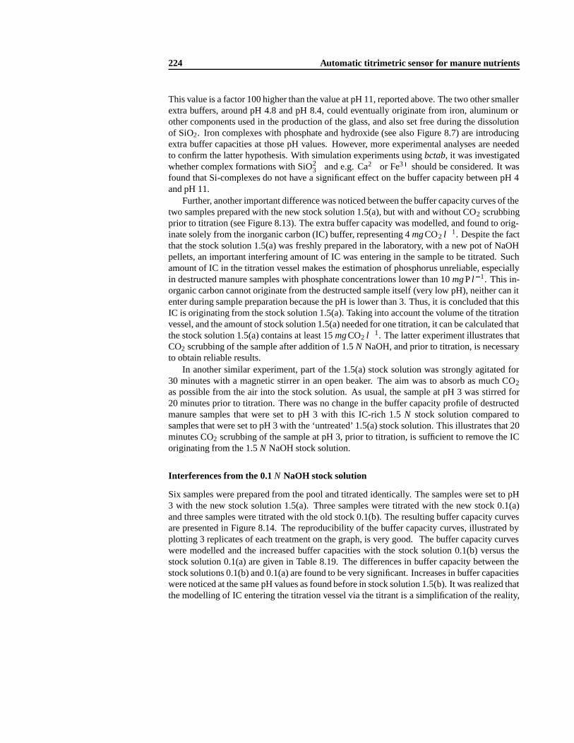
224 Automatic titrimetric sensor for manure nutrients
This value is a factor 100 higher than the value at pH 11, reported above. The two other smallerextra buffers, around pH 4.8 and pH 8.4, could eventually originate from iron, aluminum orother components used in the production of the glass, and also set free during the dissolutionof SiO2. Iron complexes with phosphate and hydroxide (see also Figure 8.7) are introducingextra buffer capacities at those pH values. However, more experimental analyses are neededto confirm the latter hypothesis. With simulation experiments using bctab, it was investigatedwhether complex formations with SiO2�
3 and e.g. Ca2+ or Fe3+ should be considered. It wasfound that Si-complexes do not have a significant effect on the buffer capacity between pH 4and pH 11.
Further, another important difference was noticed between the buffer capacity curves of thetwo samples prepared with the new stock solution 1.5(a), but with and without CO2 scrubbingprior to titration (see Figure 8.13). The extra buffer capacity was modelled, and found to orig-inate solely from the inorganic carbon (IC) buffer, representing 4 mgCO2 l�1. Despite the factthat the stock solution 1.5(a) was freshly prepared in the laboratory, with a new pot of NaOHpellets, an important interfering amount of IC was entering in the sample to be titrated. Suchamount of IC in the titration vessel makes the estimation of phosphorus unreliable, especiallyin destructed manure samples with phosphate concentrations lower than 10 mgP l�1. This in-organic carbon cannot originate from the destructed sample itself (very low pH), neither can itenter during sample preparation because the pH is lower than 3. Thus, it is concluded that thisIC is originating from the stock solution 1.5(a). Taking into account the volume of the titrationvessel, and the amount of stock solution 1.5(a) needed for one titration, it can be calculated thatthe stock solution 1.5(a) contains at least 15 mgCO2 l�1. The latter experiment illustrates thatCO2 scrubbing of the sample after addition of 1.5 N NaOH, and prior to titration, is necessaryto obtain reliable results.
In another similar experiment, part of the 1.5(a) stock solution was strongly agitated for30 minutes with a magnetic stirrer in an open beaker. The aim was to absorb as much CO2
as possible from the air into the stock solution. As usual, the sample at pH 3 was stirred for20 minutes prior to titration. There was no change in the buffer capacity profile of destructedmanure samples that were set to pH 3 with this IC-rich 1.5 N stock solution compared tosamples that were set to pH 3 with the ‘untreated’ 1.5(a) stock solution. This illustrates that 20minutes CO2 scrubbing of the sample at pH 3, prior to titration, is sufficient to remove the ICoriginating from the 1.5 N NaOH stock solution.
Interferences from the 0.1 N NaOH stock solution
Six samples were prepared from the pool and titrated identically. The samples were set to pH3 with the new stock solution 1.5(a). Three samples were titrated with the new stock 0.1(a)and three samples were titrated with the old stock 0.1(b). The resulting buffer capacity curvesare presented in Figure 8.14. The reproducibility of the buffer capacity curves, illustrated byplotting 3 replicates of each treatment on the graph, is very good. The buffer capacity curveswere modelled and the increased buffer capacities with the stock solution 0.1(b) versus thestock solution 0.1(a) are given in Table 8.19. The differences in buffer capacity between thestock solutions 0.1(b) and 0.1(a) are found to be very significant. Increases in buffer capacitieswere noticed at the same pH values as found before in stock solution 1.5(b). It was realized thatthe modelling of IC entering the titration vessel via the titrant is a simplification of the reality,

8.5 Laboratory validation and statistical data analysis 225
0
0.5
1
1.5
4 5 6 7 8 9 10
Buf
fer
capa
city
(m
eq l-1
pH
-1)
pH
Old NaOH 0.1 NNew NaOH 0.1 N
Figure 8.14: Experimental buffer capacity curves of 1 sample, titrated with an old and a newNaOH 0.1 N stock solution (a). Three replicates with each stock solution are plotted on top ofeach other
0
10
20
30
40
50
60
70
80
90
100
3 4 5 6 7 8 9 10 11
Titr
ant c
onsu
mpt
ion
(%)
pH
Figure 8.15: Typical titrant consumption profile in function of the pH for a titration with NaOHfrom pH 3 to pH 11
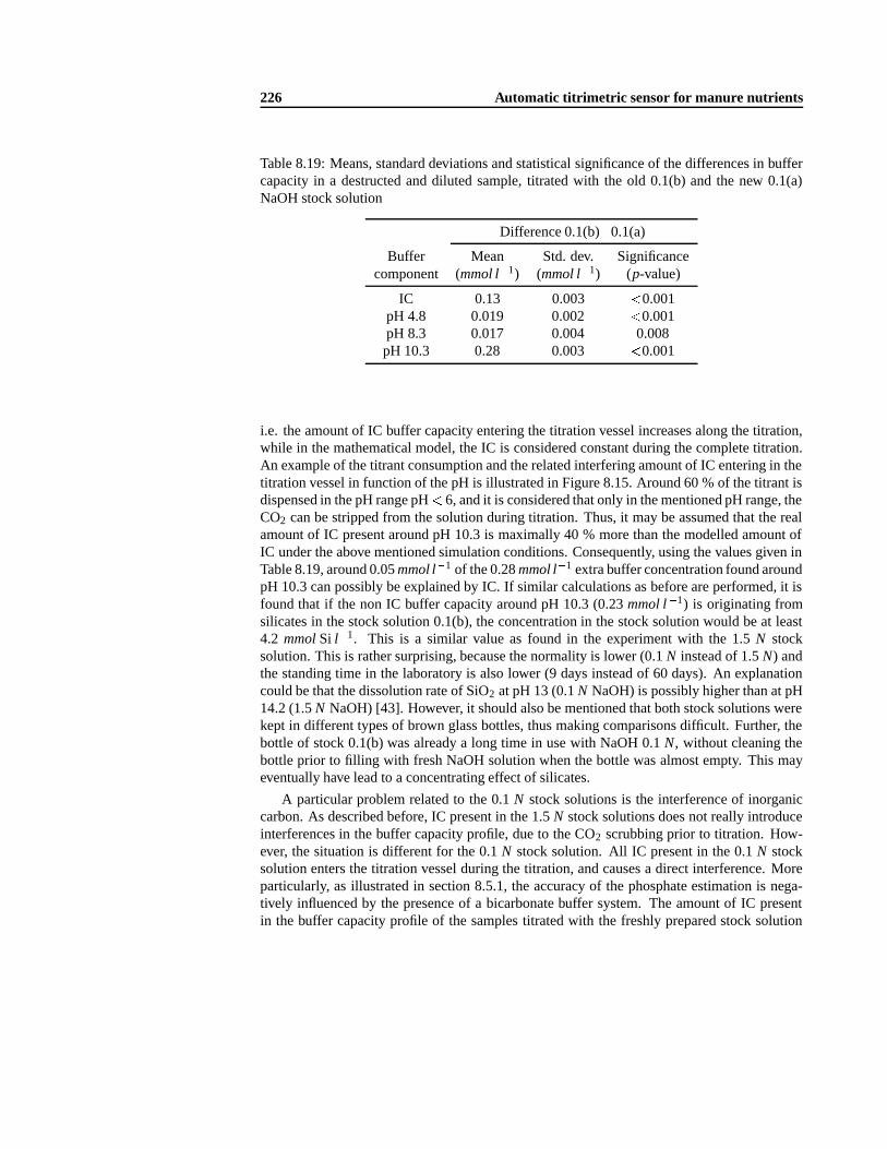
226 Automatic titrimetric sensor for manure nutrients
Table 8.19: Means, standard deviations and statistical significance of the differences in buffercapacity in a destructed and diluted sample, titrated with the old 0.1(b) and the new 0.1(a)NaOH stock solution
Difference 0.1(b)�0.1(a)
Buffer Mean Std. dev. Significancecomponent (mmol l�1) (mmol l�1) (p-value)
IC 0.13 0.003 <0.001pH 4.8 0.019 0.002 <0.001pH 8.3 0.017 0.004 0.008pH 10.3 0.28 0.003 <0.001
i.e. the amount of IC buffer capacity entering the titration vessel increases along the titration,while in the mathematical model, the IC is considered constant during the complete titration.An example of the titrant consumption and the related interfering amount of IC entering in thetitration vessel in function of the pH is illustrated in Figure 8.15. Around 60 % of the titrant isdispensed in the pH range pH < 6, and it is considered that only in the mentioned pH range, theCO2 can be stripped from the solution during titration. Thus, it may be assumed that the realamount of IC present around pH 10.3 is maximally 40 % more than the modelled amount ofIC under the above mentioned simulation conditions. Consequently, using the values given inTable 8.19, around 0.05 mmol l�1 of the 0.28 mmol l�1 extra buffer concentration found aroundpH 10.3 can possibly be explained by IC. If similar calculations as before are performed, it isfound that if the non IC buffer capacity around pH 10.3 (0.23 mmol l�1) is originating fromsilicates in the stock solution 0.1(b), the concentration in the stock solution would be at least4.2 mmolSi l�1. This is a similar value as found in the experiment with the 1.5 N stocksolution. This is rather surprising, because the normality is lower (0.1 N instead of 1.5 N) andthe standing time in the laboratory is also lower (9 days instead of 60 days). An explanationcould be that the dissolution rate of SiO2 at pH 13 (0.1 N NaOH) is possibly higher than at pH14.2 (1.5 N NaOH) [43]. However, it should also be mentioned that both stock solutions werekept in different types of brown glass bottles, thus making comparisons difficult. Further, thebottle of stock 0.1(b) was already a long time in use with NaOH 0.1 N, without cleaning thebottle prior to filling with fresh NaOH solution when the bottle was almost empty. This mayeventually have lead to a concentrating effect of silicates.
A particular problem related to the 0.1 N stock solutions is the interference of inorganiccarbon. As described before, IC present in the 1.5 N stock solutions does not really introduceinterferences in the buffer capacity profile, due to the CO2 scrubbing prior to titration. How-ever, the situation is different for the 0.1 N stock solution. All IC present in the 0.1 N stocksolution enters the titration vessel during the titration, and causes a direct interference. Moreparticularly, as illustrated in section 8.5.1, the accuracy of the phosphate estimation is nega-tively influenced by the presence of a bicarbonate buffer system. The amount of IC presentin the buffer capacity profile of the samples titrated with the freshly prepared stock solution

8.5 Laboratory validation and statistical data analysis 227
0.1(a) was modelled to be around 1:5�2 mgCO2 l�1. In a following experiment, it is verifiedif this modelled IC buffer capacity is indeed originating from CO2.
Six new titration curves were recorded with the 0.1(a) stock solution. As in the previousexperiment, all samples were prepared with the 1.5(a) stock solution, and stirred for 20 minutesprior to titration. Three different treatments, each with 2 replicates, were compared with eachother. First, a titration was performed as usual, with a closed titration vessel. Second, a titrationcurve was obtained with the titration vessel open to the air (a circular opening with a diameterof 1 cm). Third, a titration profile was recorded while N2 was continuously bubbled through thesample. There was no significant difference between the mean concentrations of IC obtainedwith the first two treatments. This indicates that it is not strictly necessary to keep the titrationvessel airtight. The amount of IC with treatment 1 and 2 was estimated to be 1.8 mgCO2 l�1.A very significant difference (p = 0:01) in IC was found between treatment 3 and the firsttwo treatments. The estimated amount of IC in treatment 3 was 1.0 mgCO2 l�1. Thus, 0.8mgCO2 l�1 from the 1.8 mgCO2 l�1 is removed by the N2 bubbling, and is considered as IC.It is uncertain if the remaining amount of buffer capacity (1 mgCO2 l�1) is originating fromIC, or resulting from other buffer systems in the same pH range of IC.
The discussed interferences (IC and non-IC) are directly related to the accuracy and pre-cision of the ammonium and ortho-phosphate estimations from the buffer capacity profile.Therefore, they should be kept as low as possible. To get more insight in these interferencesand to find possible solutions or alternatives, further experiments are presented in the nextparagraph.
Validation and alternatives
A new experiment was designed to confirm and extend the findings of the experiments previ-ously described in this section. More particularly, the objectives of this experiment are to:
� Validate whether silicate dissolution from the glass bottle containing the 0.1 N NaOHtitrant is responsible for the interfering buffer capacity found around pH 10.
� Determine whether the IC found in the buffer capacity profiles (estimated 0.8 mgCO2 l�1
in the previous experiment) is originating from the NaOH 0.1 N stock solution, or ratheroriginating from the CO2 in the headspace of the titration vessel.
� Evaluate the performance of commercially prepared NaOH solutions, stored in com-pletely closed, headspace free plastic bags (Titripack , Merck).
A new pool of destructed manure samples was made, to be able to titrate the same sampleunder varying conditions. Sample preparations and titrations were performed as before. Tobring the sample to pH 3, NaOH 1 N (Titripack ) was used. Three different stock solutionsNaOH 0.1 N were used for the titrations from pH 3 to pH 11:Stock 0.1(c) : One litre of NaOH solution was prepared with NaOH pellets from an almost
empty pot ‘NaOH pro analyse’ (the same pot as used in the previous experi-ment for solution 0.1(b)). Half of this freshly prepared solution was kept in acompletely closed glass bottle for 9 days at room temperature. After this ‘ in-cubation period’ , the bottle was connected as usual to the titrator (with CO2
scrubber) and used for the titrations.

228 Automatic titrimetric sensor for manure nutrients
Stock 0.1(d) : The other half litre of the freshly prepared NaOH was kept in a completelyclosed plastic bottle for 9 days prior to titration.
Stock 0.1(e) : A commercial NaOH 0.1 N 10 litre stock solution (Titripack , Merck).With each of these stock solutions, three different treatments, each in threefold, were ap-
plied for titrations of destructed and diluted manure samples from the pool:
� titration as usual, in a closed titration vessel,� titration while bubbling N2 through the liquid, and� titration while flowing N2 through the headspace of the vessel.
The exact titres of the stock solutions were determined with oxalic acid titrations. Despitethe fact that solution 0.1(c) and 0.1(d) should theoretically have the same titre, the normalityof solution 0.1(c) after nine days incubation in the glass bottle was 0.7 % lower than the nor-mality of the same solution kept in the plastic bottle. This difference is small, but was foundto be statistically significant (p < 0:001). Further, the buffer capacity curves obtained withthe 3 different titrant solutions were compared to confirm the hypothesis that silicates or othersubstances enter the stock solution kept in the glass bottle. Rather surprisingly, the extra buffercapacity expected around pH 10 or elsewhere was not found in the titration curves obtainedwith solution 0.1(c). When using the most adequate mathematical model (see section 8.4.7)on the titration curves obtained with N2 bubbling in the liquid, no significant differences werefound in the estimated N and P concentrations resulting from titrations with the 3 differentNaOH stock solutions (on the α = 0:01 level). This means that the earlier formulated hypoth-esis of the silicate interference is not valid here. A possible explanation could be that in theprevious experiment, stock solution 0.1(b) was the result of a longer than 9 days ‘aging period’due to the bottle refilling method used in many previous experiments. When the glass bottleof the titrant solution 0.1 N was almost empty (e.g. 10 % of the volume left), the bottle wasrefilled (without emptying and cleaning) with freshly prepared NaOH solution. Thus, stocksolution 0.1(b) was kept in a glass bottle that was continuously exposed to NaOH for at least3 weeks. It was also noticed in the past that titration curves obtained with titrant of an almostempty titrant bottle are often ‘noisy’ and not very reproducible. This points to possible con-centrating interferences at the bottom of bottle. Extra results, from longer ‘ incubation’ times,are presented further in this section.
To evaluate the origin of IC in the buffer capacity profiles, the effect of the 3 different treat-ments on the IC was investigated with an analysis of variance (GLM). First, the buffer capacitycurves of the samples with N2 bubbling in the liquid were modelled with the most adequatemathematical model (see section 8.4.7). As mentioned above, no significant differences werefound in N and P estimations obtained with the 3 different NaOH titrant solutions. Second,the estimated concentrations of N and P were kept fixed in a new model, that was fitted to the27 buffer capacity curves (3 titrant solutions, 3 treatments, 3 replicates), with the purpose of amore correct estimation of the IC. The mean IC concentrations found with this model are tab-ulated in Table 8.20. The residual standard deviation on the IC concentrations, obtained fromthe GLM analysis, was 0.15 mgCO2 l�1. From pairwise comparisons in the GLM analysis,it was concluded that there is no significant difference in IC between titrant 0.1(c) and 0.1(d).The IC found with titrant 0.1(e) was found to be significantly different from the 2 other NaOHsolutions. There was no significant interaction between the effect of the titrant solution andthe effect of the treatments. Further, among the 3 treatments, all were found to be significantly
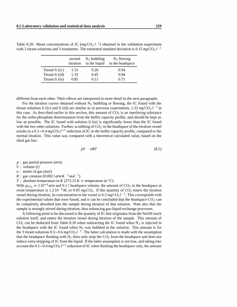
8.5 Laboratory validation and statistical data analysis 229
Table 8.20: Mean concentrations of IC (mgCO2 l�1) obtained in the validation experimentwith 3 titrant solutions and 3 treatments. The estimated standard deviation is 0.15 mgCO2 l�1
normal N2 bubbling N2 flowingtitration in the liquid in the headspace
Titrant 0.1(c) 1.33 0.26 0.94Titrant 0.1(d) 1.33 0.45 0.94Titrant 0.1(e) 0.85 0.11 0.71
different from each other. Their effects are interpreted in more detail in the next paragraphs.For the titration curves obtained without N2 bubbling or flowing, the IC found with the
titrant solutions 0.1(c) and 0.1(d) are similar as in previous experiments, 1.33 mgCO2 l�1 inthis case. As described earlier in this section, this amount of CO2 is an interfering substancefor the ortho-phosphate determination from the buffer capacity profile, and should be kept aslow as possible. The IC found with solution 0.1(e) is significantly lower than the IC foundwith the two other solutions. Further, scrubbing of CO2 in the headspace of the titration vesselresults in a 0.1�0.4 mgCO2 l�1 reduction of IC in the buffer capacity profile, compared to thenormal titration. This value was compared with a theoretical calculated value, based on theideal gas law:
pV = nRT (8.5)
p : gas partial pressure (atm)V : volume (l )n : moles of gas (mol)R : gas constant (0.082 l atm K�1 mol�1)T : absolute temperature in K (273.15 K + temperature in oC)With pCO2 = 3 10�4 atmand 0.1 l headspace volume, the amount of CO2 in the headspace atroom temperature is 1:2 10�6 M, or 0.05 mgCO2. If this quantity of CO2 enters the titrationvessel during titration, its concentration in the vessel is 0.3 mgCO2 l�1. This corresponds withthe experimental values that were found, and it can be concluded that the headspace CO2 canbe completely absorbed into the sample during titration of that solution. Note also that thesample is strongly stirred during titration, thus enhancing gas-liquid exchange processes.
A following point to be discussed is the quantity of IC that originates from the NaOH stocksolution itself, and enters the titration vessel during titration of the sample. This amount ofCO2 can be deducted from Table 8.20 when subtracting the IC found when N2 is injected inthe headspace with the IC found when N2 was bubbled in the solution. This amount is forthe 3 titrant solutions 0.5�0.6 mgCO2 l�1. The latter calculation is made with the assumptionthat the headspace flushing with N2 does only strip the CO2 from the headspace and does notinduce extra stripping of IC from the liquid. If the latter assumption is not true, and taking intoaccount the 0.1�0.4 mgCO2 l�1 reduction of IC when flushing the headspace only, the amount

230 Automatic titrimetric sensor for manure nutrients
of IC originating from the titrant is estimated to be between 0.6 and 1 mgCO2 l�1.Another finding of this experiment is that the modelled amount of IC with titrant solutions
0.1(c) and 0.1(d) is always higher than the concentration found with solution 0.1(e). Especiallyfrom the treatment with N2 bubbling in the liquid, it can be concluded that higher amountsof buffering interferences, not stripped off by N2 bubbling, are originating from the NaOHsolutions 0.1(c) and 0.1(d) compared to solution 0.1(e).
From the results described above, it can be concluded that the NaOH solution 0.1(e), i.e. thecommercial Titripack NaOH solution gives more reliable and more accurate titration resultscompared to NaOH 0.1 N solutions prepared in the lab. Because the Titripack plastic bagsare completely closed and headspace free, it is also expected that interferences are smaller andmore constant in function of time, making it easier to incorporate them in the mathematicalbuffer capacity models. There are two more advantages of this Titripack solutions that werenot mentioned before. First, these solutions have an exact titre (deviation from 0.1 N is maxi-mum 0.02 %), which eliminates the necessity to determine the normality with e.g. oxalic acidtitrations. Second, these solutions are degassed, and consequently, no air bubbles are formedon the moving piston of the titrator burette. Such air bubbles appear quickly when self preparedNaOH solutions are used (NaOH pellets and demineralized water). When such an air bubblereleases the piston, it induces a titrant dosing error. There is, however, a major price differencebetween Titripack solutions (e 8.5 per litre NaOH 0.1 N) and self prepared NaOH 0.1 N solu-tion (e 0.05 for NaOH pro analyse pellets and e 0.5 for demineralized water per litre of NaOH0.1 N). Taking into account the extra products and working hours necessary to prepare stocksolutions and determine the exact titre with e.g. oxalic acid titrations, the price difference isnot an obstruction any more. For example, to prepare 1 litre of NaOH 0.1 N and determinethe exact titre with an oxalic acid end-point titration in 4 replicates, it costs 15 minutes labour(e6) and 2 hours occupation of an automatic laboratory titrator with sample carousel (roughlyestimated at e 4).
Because it was considered important to validate the hypothesis of the silicate dissolutionin the NaOH titrant, the validation experiment was extended, and a longer incubation period(20 days) was tested with solution 0.1(c). Also, the SiO2 dissolution rate is highly temperaturedependent [43], thus part of the 0.1(d) stock solution, previously not in contact with glass,was kept at 45 oC in a closed glass bottle for 4 days. Summarizing, extra titration curves wereobtained with
� Stock 0.1(c), kept for 20 days in a closed brown glass bottle at room temperature.� Stock 0.1(d), kept for 16 days in a closed plastic bottle at room temperature, and then
transferred into a completely closed brown glass bottle at 45 oC for 4 days.
With these stock solutions, destructed and diluted samples from the pool were titrated oncenormally and in threefold while bubbling N2 in the liquid. Buffer capacity curves obtainedwith titrant solutions 0.1(e) and 0.1(d) are given in Figure 8.16. The curves obtained withsolution 0.1(c) are very similar to the curves obtained with solution 0.1(d) and are thereforenot shown in Figure 8.16.
The results were compared with the previous titration experiments, and similar buffer ca-pacity increases around pH 10 were found with both stock solutions 0.1(c) and 0.1(d). Thus, itwas concluded that an aging period of 20 days, or an aging period of 4 days at elevated temper-ature, introduces significant amounts of extra buffers into the stock solution. These increases

8.5 Laboratory validation and statistical data analysis 231
0
0.2
0.4
0.6
0.8
1
1.2
4 5 6 7 8 9 10
Buf
fer
capa
city
(m
eq l-1
pH
-1)
pH
Titripack NaOH 0.1 N (1)Self prepared NaOH 0.1 N, 20 days old (1)Self prepared NaOH 0.1 N, 20 days old (2)
Figure 8.16: Experimental buffer capacity curves of 1 sample, titrated with a Titripack andself prepared NaOH 0.1 N stock solution, with (1) and without (2) CO2 scrubbing duringtitration. For the treatments (1), three replicates with each stock solution are plotted on top ofeach other
were quantified to be around 9 10�5 M. As discussed before, part of this extra buffer capacitycan originates from IC entering continuously in the titration vessel, and not completely ac-counted for in the mathematical model. If this extra buffer capacity is originating from SiO2
dissolution, the concentration in the stock solution would be maximally 1.9 mmolSi l�1 or54 mgSi l�1. Taking into account the dimensions of the bottle (0.02 m2 liquid-glass contactsurface and 0.2 l titrant) and the standing period (20 days), it is calculated that the dissolutionrate of SiO2 would be 3:8 10�5 mol m�2 h�1. This is again the same value as found before.Finally, laboratory analyses of the amount of silicates in both stock solutions at the end of allexperiments were performed (molybdenum blue colorimetric method). These found respec-tively 52 and 67 mgSi l�1 in stock solutions 0.1(c) and 0.1(d). As an extra verification, thequantity of Si in stock solution 0.1(e) (Titripack ) was also determined, and found to be lessthan 0.5 mgSi l�1. The high quantity of Si in stock solutions 0.1(c) and 0.1(d) clearly confirmsthe hypothesis of the silicate dissolution and its interference in the buffer capacity profiles.
Conclusions
A number of conclusions and precautions with respect to the stock solutions 1.5 and 0.1 NNaOH can be summarized as follows:
� Inorganic carbon present in the NaOH stock solution 1.5 N does not interfere with theN and P estimations from the buffer capacity profile, as long as the sample is made CO2
free at pH 3 by stirring, prior to titration with NaOH 0.1 N.

232 Automatic titrimetric sensor for manure nutrients
� Very important interferences were found in ‘aged’ stock solutions 1.5 N (2 months old)and 0.1 N (9 days old, however in a bottle that was a couple of weeks in use with NaOH,without completely emptying and cleaning). The main interfering buffer was foundaround pH 10 and was quantified as 1.5�5 mmol l�1 of an extra monoprotic buffer. It ishypothesized that this extra buffer is a silicate buffer originating from SiO2 dissolutionof the glass bottle. An extra validation experiment under similar conditions, as well aslaboratory analyses of Si in ‘aged’ stock solutions clearly confirmed this hypothesis.
� Inorganic carbon buffer capacity interferes with the ortho-phosphate determination, andshould be kept as low as possible. Under normal titration conditions, the amount of ICthat can enter the solution via a 100 ml headspace is 0.3 mgCO2 l�1. The amount of ICthat enters the titration vessel via the titrant solution is around 0.5�0.6 mgCO2 l�1.
� If the interfering amount of IC would be constant, its influence can easily be corrected byaccounting this amount of IC in the mathematical buffer capacity model. Otherwise, theortho-phosphate overestimation error from the buffer capacity profile could be around0.4 mgP l�1 diluted sample or 3 mgP l�1 undiluted destructed sample.
� The titration vessel does not have to be completely closed to obtain reliable results. Nosignificant differences were found between buffer capacity profiles obtained in a closedvessel, and in an open to the air vessel (opening of 1 cm2).
� The commercial NaOH 0.1 N solution (Titripack , Merck) was evaluated and foundmore reliable (less sensitive to possible contaminations), more accurate and containingless interferences than self prepared NaOH stock solutions. A price comparison wasmade, and it was concluded that Titripack solutions are not necessarily more expensivethan self prepared stock solutions.
8.5.3 Statistical data analysis
The results of the validation experiment described in section 8.5.1 were statistically evalu-ated, and the different sources of variability were quantified and interpreted. The investigatedsources of variability are the method variability (laboratory versus titrimetric result), the du-plo variability (2 subsamples from each raw manure sample are analyzed) and the residualvariability (uncontrolled variability due to sample preparation, titration, data analysis, : : : ).
The available data for this study originates from 53 different manure samples. From eachmanure sample, 2 subsamples (or duplos) of approximately 5 g were taken. The exact weightof each subsample was recorded, because this weight factor is needed to transform the ana-lytical results from mg l�1 destructed sample to mg kg�1 manure, in which the final resultsshould be expressed. The subsample weight typically varies between 4 and 6 g, and the duplovariability can only be investigated when this weight factor is included in the statistical anal-yses. Therefore, the statistics are performed on data expressed as mg kg�1. Each subsamplewas analyzed once in the laboratory for N and P with the official NEN methods. Further, eachdestructed subsample was diluted and titrated in threefold, thus resulting in 3 independentlyestimated N and P concentrations for each subsample. Later, 20 subsamples (originating from12 samples with P < 10 mg l�1 in destructed, undiluted sample) were repeated because of theinterferences discussed in section 8.5.2. There was not enough sample left to include replicatetitrations, thus each of the 20 repeated subsamples was titrated only once.
An introductory remark that should be made prior to statistical interpretations, is that the

8.5 Laboratory validation and statistical data analysis 233
Table 8.21: Duplo and residual variability analysis obtained with two GLM’s for respectivelythe laboratory and the titrimetric data
Source of Significance Mean X Std. dev. sX r.s.d.Variable variation Method (p-value) (mg kg�1) (mg kg�1) (%)
N53 duplo laboratory 0.007 4941 14 0.3N53 duplo titrimetric 0.01 4898 21 0.4P41 duplo laboratory 0.09 1361 3.7 0.3P41 duplo titrimetric 0.001 1318 30 2.3P12 duplo laboratory 0.008 246 2.4 1.0P12 duplo titrimetric 0.13 247 15 6.1N53 residual titrimetric 4898 64 1.3P41 residual titrimetric 1318 54 4.1P12 residual titrimetric 247 37 15
data set is highly unbalanced, because no replicate analyses were available for the laboratorymeasurements compared to the threefold titrimetric measurements. Therefore, it was chosenin a first stage to assess the duplo variability on the laboratory data, and the duplo plus residualvariability on the titrimetric measurements, with two separate GLM studies. The variables thatwere investigated areN53 : Ammonium on all of the 53 samplesP41 : Ortho-phosphate on 41 samples with P > 10 mg l�1
P12 : Ortho-phosphate on 12 repeated samples with P < 10 mg l�1
The duplo effect and the sample effect were included as two random factors in the GLM.For the titrimetric data, an interaction effect sample�duplo was also included in the GLM.Summarized results are given in Table 8.21. The duplo variability, expressed as a standarddeviation, can be interpreted as follows: If many subsamples originating from 1 sample areanalyzed either in the laboratory or with the titrimeter, 95 % of the results are expected inthe interval X� 2sduplo. 2 Similarly, for the residual variability of the titrimetric measure-ment: If one subsample is titrated many times, 95 % of the results are expected in the intervalX�2sresid. Theoretically, the duplo variability is expected to be the same with both measure-ment methods. This is fairly well the case, except for P41 and P12, where the duplo standarddeviations are found to be higher in the titrimetric method. The duplo variability, expressedas r.s.d., is between 0.3 and 1 % for the laboratory measurements, which confirms that thesubsampling is a reproducible process. The titrimetric reproducibility was evaluated, and itwas found that the titrimetric variability is homogeneous along the range from low loaded tohigh loaded samples (homoscedasticity). This is also reflected when comparing the residualstandard deviation of P41 and P12. As a logical consequence, the relative error in the lowloaded P samples is higher (15 %) compared to the high loaded P samples (4.1 %). The re-
2The latter statement is somewhat simplified, because the effect of the residual variability should also beconsidered.

234 Automatic titrimetric sensor for manure nutrients
Table 8.22: Method variability analysis obtained with paired t-tests for laboratory versus titri-metric analyses results
Paired differences (lab. � titrimetric) (mg kg�1)
Variable Nbr. of pairs Sign. Mean d Std. dev. sd 95 % conf. interval of d
N53 106 <0.001 43 95 25�61P41 82 0.001 43 115 18�68P12 20 0.91 �0:97 37 �18�16
producibility of the ammonium estimation with the titrimeter is very good, 1.3 %. Such lowresidual error indicates that further optimization of the titrimetric reproducibility is not neededfor the ammonium measurement. However, the situation is different for the ortho-phosphatereproducibility. This is in correspondence with earlier experimental findings, that the buffercapacity of ortho-phosphate is much more influenced by external uncontrolled factors, in thefirst place the inorganic carbon. A quick calculation learns that a residual ortho-phosphatestandard deviation of 37 mg kg�1 manure corresponds with an ortho-phosphate concentrationin the titration vessel of 0.11 mgP l�1, or 0.004 mmol l�1. A typical amount of IC entering thetitration vessel via the headspace and the titrant is 1 mgCO2 l�1, or 0.02 mmol l�1. Hence, themolar amount of interfering IC is 5 times higher than the amount of phosphate representing theresidual standard deviation. Thus, further optimization of the titrimetric procedure, to keep theIC as low and as constant as possible, is the strategy to be followed to decrease the variabilityof the titrimetric P measurement.
In a second stage, the method variability (laboratory versus titrimetric) was investigated.Therefore, in the second stage, it was chosen to aggregate the replicate titrimetric measure-ments and calculate their means as values for a new data set. The aggregated and thus balanceddata set contains 53 samples, each with 2 subsamples (duplos), and each subsample has onelaboratory and one titrimetric N and P measurement. A GLM with 1 fixed factor (method) and2 random factors (sample and duplo) was constructed. Three main effects and three two-wayinteractions were included in the model and could be interpreted. Only for P12, the interpre-tation is simple and straightforward: None of the interactions are significant, and there are nosignificant effects of duplo and method. In other words, the P12 results of the laboratory are notstatistically different from the titrimetric results. For N53 and P41, the interpretation is morecomplicated. The interactions method�sample and method�duplo are very significant, thusmasking possible interpretation of the main effect ‘method’ . The method effect should be in-terpreted as significant through its interactions with the two random factors. In other words, itis concluded that this GLM study cannot be used to give a simple and clear answer to the ques-tion whether the laboratory and titrimetric results are significantly different from each otherfor N53 and P41.
In a third stage, another approach was followed to specifically interpret the method effect.Based on the results of the previous stage, a paired t-test was chosen as the best option to eval-uate the method effect. The summarized results of these tests are given in Table 8.22. From

8.5 Laboratory validation and statistical data analysis 235
Table 8.23: Official accreditation requirements for the measurement of nitrogen and phospho-rus in animal manure [1] compared with the obtained results
Required Obtained
Minimum measurable concentration N 150 mg kg�1 190 mg kg�1
Minimum measurable concentration P 40 mg kg�1 110 mg kg�1
Reproducibility N (0�2500 mgNkg�1) 150 mg kg�1 67 mg kg�1
Reproducibility N (> 2500 mgNkg�1) 6 % relative 1.4 % relativeReproducibility P (0�500 mgPkg�1) 40 mg kg�1 40 mg kg�1
Reproducibility P (> 500 mgPkg�1) 8 % relative 3.6 % relative
these results, it is concluded that there is a significant difference between the laboratory andtitrimetric measurements for N53 and P41. In both cases, the mean laboratory values are higherthan the titrimetric results. For the repeated samples, P12 is not significantly different for bothmethods. This can partially be explained because in the low loaded samples, the mean concen-tration for P is much lower compared to the high loaded samples, thus for the same residualvariability, it is statistically more difficult to find significant differences in the lower range. Theconfidence intervals in Table 8.22 are best suitable to interpret the difference in results betweenthe laboratory and the titrimetric measurement. E.g. if many samples are analyzed in the lab-oratory and with the titrimeter, the mean difference in ammonium concentration (laboratory�titrimetric) will be with 95 % confidence between 25 and 61 mg kg�1.
Finally, the obtained statistical results were compared with the requirements for an officialaccreditation in the Netherlands [1] for nitrogen and phosphorus measurement in animal ma-nure. These requirements include the minimum measurable concentration (expressed as threetimes the residual standard deviation sX) and the reproducibility (including the subsampling orduplo effect and the analysis effect). The obtained results are calculated from Table 8.21. Theaccreditation requirements and the obtained results are summarized in Table 8.23.
The obtained minimum measurable concentrations N and P, calculated from the residualstandard deviations of the titrimetric measurements are still higher than the required values. Es-pecially for P, the results are not fully acceptable yet. However, it should be taken into accountthat the titrimetric data used in this validation study (see section 8.5.1) were obtained withoutappropriate control and minimizations of the interferences discovered afterwards (silicates andIC). Therefore, taken into account the results obtained in section 8.5.2, it is expected that bytaking care of the described interferences, the minimum measurable concentrations for N andP will be within the requirements for accreditation. The obtained reproducibility (includingthe effects of subsampling and analysis) is already within the requirements.
A recent but unofficial comparative study among 8 different Dutch laboratories for N andP measurement in one pig manure sample has been organized by a pig farmers association [2].This small scale study showed differences between the minimum and maximum reported anal-ysis results of 24 % and 87 % for respectively N and P. A similar comparative test in Flanders(called ‘ ringtest’ ) [64] in which 30 laboratories were involved, found differences between the
236 Automatic titrimetric sensor for manure nutrients
minimum and maximum reported analysis results of 54 % and 39 % for respectively N andP. This official test was also used in an accreditation procedure to select the laboratories thatare officially allowed to perform these measurements. From these two recent studies, one canconclude that nutrient measurements in manure are sensitive to many sources of error whichare in some of the tested laboratories not completely under control yet.
8.6 Conclusions
The final goal of the FASTNAP project is to build a functional model of the device. Thishardware model should be able to demonstrate the functionality of an automatic and on-lineN and P measurement in manure samples. In the current stage of the project, the functionalmodel will be constructed on a non-driving vehicle. However, in a further post-project stage,the aim is to have measurements conducted on a driving vehicle. Within this framework, thetechniques used in the project were chosen in function of this ultimate goal. The followedmethodology can be summarized in four consecutive steps. First, a representative manuresample is taken from a transporting vehicle during loading or unloading of the vehicle. Thisis existing technology, and available on the market. This sample is homogenized and a sub-sample is taken (5 ml out of 750 ml manure). Second, the sample is destructed with the aid ofchemicals and heat (microwave oven). Third, a titration curve is recorded from pH 3 to pH 11.And last, an advanced data-processing step, based on buffer capacity modelling, is performed.The development of the latter two steps was the main topic of this chapter.
The official NEN 7433 manure destruction procedure includes the addition of CuSO4 �5H2O as a catalyst. However, this high amount of Cu2+ caused an interfering precipitationreaction with o-PO4 during titration, such that it was investigated if this catalyst is really nec-essary to obtain a complete destruction of the animal manure. It was found that this catalystcould be omitted, and therefore, all further destructions in the framework of this project wereperformed without the Cu catalyst.
Destructed manure samples contain in order of importance: sulphuric acid, ammonium,ortho-phosphate, calcium, potassium, iron, and a whole range of minor elements. The effectof ionic strength on the buffer capacity is important, and ionic activity corrections should beincluded in the mathematical models. The effect of dilution of the destructed manure sampleprior to titration was investigated. Undiluted or too much diluted destructed manure samplesgive unreliable titration results, and a dilution factor between 3 and 6 was experimentallyfound to give the best results. The effect of simple chemical equilibrium reactions can easilybe modelled, and it is also straightforward to include complexation reactions in a mathematicalmodel for buffer capacity of destructed manure. Complexation reactions with Ca2+ and Fe3+
were investigated in more detail, and it was found that iron and calcium complexes couldbe responsible for buffer capacities around pH 5, pH 8 and pH 10. It was also found thatthe buffer capacities of o-PO4 and NH+
4 (the buffers of main interest) are only influenced bythe complex formation reactions to a limited extent. Possible precipitation reactions duringtitration were also investigated with simulation studies, and a number of potential precipitateswere found. However, literature research learned that precipitation reactions are sluggish, slow,non-stoichiometric, incomplete, : : : Simulation studies with precipitation reactions includedlearned that their effect is negligible for ammonium and ortho-phosphate estimation. It was

8.6 Conclusions 237
chosen for the further model developments to exclude precipitation reactions from the models.A first measurement campaign was organized for the development of an adequate buffer
capacity model. Titrimetric N and P estimations were compared with laboratory results usingstandard NEN methods. Four selected mathematical models were compared with each other,and it was found that the best N and P estimations are obtained with a rather simple model,only including buffer capacities originating from H2O, H2SO4, IC, o-PO4 and NH+
4 . With thismodel, a lack of fit was observed due to extra experimental buffer capacity found around pH 5.5and pH 8. Referring to the simulation study, these extra buffer capacities could be attributed tothe complex formation reactions. With another model, that took those 2 extra buffers into ac-count, the estimations of o-PO4 were, however, slightly worse compared to the most adequatemodel. A correlation study between the concentrations of these extra two buffers and the con-centrations of the most important components in destructed manure confirmed the hypothesisof the complexation reactions at these two pH ranges.
A second measurement campaign (53 samples, 2 subsamples, 3 replicates) was organizedto validate the most adequate buffer capacity model. Also for the new data set the developedmodel was optimal. This points to the robustness of this model in different situations. Theammonium concentrations found with the titrimetric analyses are all between �7 and +8 %relative error compared to the laboratory measurements. The relative errors for the titrimetricortho-phosphate concentrations are between �25 and +200 % compared to the laboratorymeasurements. The highest deviations were noticed for the 20 % lowest loaded P samples(or P < 10 mg l�1). A number of interferences originating from the NaOH stock solutionswere found to be the reason of the high relative errors particularly for P. The low loaded Psamples were titrated again, using freshly prepared NaOH stock solutions, and the relativeerrors became in an acceptable range between �15 and +25 % compared to the laboratoryresults.
The influences of the alkaline stock solutions were investigated in more detail with separateexperiments to characterize and quantify the interfering buffers in the NaOH stock solutions.There are two different interfering substances that should be kept as low and constant as pos-sible. The first one is IC, found to originate from the stock solution 0.1 N and the headspaceof the titration vessel. Its quantity is typically around 1 mgCO2 l�1, and causes an impor-tant interference for the ortho-phosphate determination in case it is not known or not constant.The second interfering substance is found to originate from SiO2 dissolution from the glassbottle where the alkaline stock solution was kept. Its quantity is around 1.5 mmol l�1 in 20days old stock solutions of NaOH 0.1 N. This interfering amount of silicates interferes withthe ammonium estimation. It is concluded that commercially prepared NaOH stock solutions(Titripack , Merck) are a strong and reliable alternative to avoid interferences, both from ICand silicates. These solutions are stored in completely closed, headspace free plastic bags of10 l , and are not necessarily more expensive than self prepared stock solutions.
A detailed statistical analysis of the data obtained with the second measurement campaignwas performed to quantify and interpret the different sources of variability. It was found thatthe duplo or subsampling variability is low, pointing to reproducible subsampling. The relativeresidual standard deviation obtained with the titrimetric measurements is 1.3 % for ammonium,and between 4 and 15 % for ortho-phosphate. This indicates that further optimization of thetitrimetric reproducibility for ortho-phosphate should be considered. Especially when the inter-ferences discussed in the previous paragraph are avoided, it is expected that the reproducibility

238 Automatic titrimetric sensor for manure nutrients
and accuracy will still become better.The goal of the project was to develop an automatic technique for N and P measurements
in animal manure in the field. Taking into account some further optimizations discussed above,the analysis results with this titrimetric sensor are expected to be as reliable as the laboratoryresults. A first comparison between the obtained results and the requirements for accredita-tion was performed, and it was concluded that the developed methodology is promising forofficial acceptance. Thus, it can even be suggested to implement the titrimetric measurementtechnique in the laboratory, with a laboratory titrator, coupled to a computer, as a reliable al-ternative for the classical laboratory methods. The strongest points of the titrimetric methodare: simultaneous N and P measurement with 1 method, minor sample manipulations, N andP results within 30 minutes, low and inexpensive chemical consumption, consumption of onlyone and non-hazardous reagent (NaOH) and the possibility to measure continuously in the labwith a sample carousel coupled to the titrating unit.

Chapter 9
Automatic pH buffer capacitymodel building
Some of the results of this chapter are submitted for the conference “Watermatex 2000” [309].
9.1 Introduction
In the previous chapters, user-defined buffer capacity models were fitted to various experimen-tal buffer capacity data, with the aim to quantify the concentration of known buffer systemsdefined in the mathematical buffer capacity model. At that stage, the interpretation of thegoodness of fit of the model still was a manual process. If necessary, the mathematical modelwas extended or modified and refitted to the data. In each chapter, an adequate field-usablemodel was developed. More particularly, models were formulated for river and effluent sam-ples (chapter 6), samples from algal wastewater treatment systems (chapter 7) and destructedand diluted animal manure samples (chapter 8).
The aim of this chapter is to automate the process of buffer capacity model building, andfind an useful and adequate buffer capacity model, tailor-made for each individual sample.Such approach is expected to yield useful information in the framework of alarm generation,because for example, the appearance of unexpected buffers (e.g. pollutants) in the buffer ca-pacity profile would be automatically detected and their characteristics quantified. In situationswith a lack of a priori knowledge about the buffers present in a titrated sample, an automaticbuffer capacity model building environment can be useful to find an appropriate model for thatsample.
The tools needed for the automatic buffer capacity model development are implementedin the software bomb, which is described in detail in section 5.3 on page 117. In this context,the automatic model building algorithm (see section 5.3.4 on page 125) and the implementedbuffer capacity model selection criteria (see section 5.3.5 on page 131) are of prior importance.
In section 9.2, a number of titration curves of samples with well-known composition willbe used to evaluate the model building algorithm and the model selection criteria. Based onthese results, a model building strategy will be formulated. In sections 9.3, 9.4 and 9.5, the

240 Automatic pH buffer capacity model building
Table 9.1: Chemicals for the preparation of samples of which titration curves were collected
Chemical Code Protonicity pKa1 pKa2 pKa3
Oxalic acid oxa 2 1.23 4.19Sodium acetate ace 1 4.75Ammoniumchloride amm 1 9.20Malonic acid mal 2 2.83 5.69Sodium tripolyphosphate pho 3 2.12 a 7.21 a 12.67 a
Citric acid cit 3 3.14 4.77 6.39a Values of ortho-phosphate. The real values have to be determined experimentally.
automatic model building environment will be evaluated with titration curves presented earlierin chapters 6, 7 and 8 respectively. An important aspect that will be investigated and discussedin this chapter is the benefit of automatic model building compared to the use of fixed buffercapacity models.
9.2 Buffer capacity modelling of well-known samples
9.2.1 Materials and methods
A number of titration curves with known composition were collected in the framework of ad-equate buffer capacity model development. The titration data collection is described in [202].Initially, a manual model building algorithm was evaluated in [202]. The goodness of fit wasinterpreted visually and the ‘best’ model was compared with the ‘ theoretical’ model. Later, thismodel building algorithm was modified and automated in [299]. Also, automatic model selec-tion criteria were introduced in [299]. Finally, based on the experiences in [202, 299], somefurther modifications to the algorithm were proposed and finally implemented in the softwarebomb, presented in section 5.3 on page 117.
The database contains 146 titration curves, originating from 66 different samples, eachtitrated in two- or threefold. The chemicals that were used to prepare the samples are presentedin Table 9.1. Four different concentrations of each chemical were used for the preparation ofthe samples: 0.5, 1, 2 and 5 meq l�1. First, samples were prepared with only 1 component,and with each of the concentrations mentioned above (in total 24 samples). Second, com-binations of 2 components were made: being oxa�amm, amm�ace, oxa�ace, pho�amm,pho�ace, oxa�mal, cit�ace, pho�mal and cit�mal. Each combination was prepared in theconcentrations 1�1, 0.5�1 and 1�0.5 meq l�1 (in total 27 samples). Third, combinationsof 3 components were formed: being oxa�amm�ace and pho�amm�cit in the concentra-tions 0.5�1�0.5, 0.5�0.5�1, 1�0.5�0.5 and 1�1�1 meq l�1 (in total 8 samples). Fourth,the combination oxa�pho�amm�ace was prepared in the concentrations 1�0.5�0.5�0.5,0.5�1�0.5�0.5, 0.5�0.5�1�0.5, 0.5�0.5�0.5�1 and 1�1�1�1 meq l�1 (in total 5 sam-ples). Fifth, the combination oxa�pho�amm�ace�cit was prepared in the concentration 0.5

9.2 Buffer capacity modelling of well-known samples 241
meq l�1 for each component. Sixth, the combination oxa�pho�amm�ace�cit�mal was pre-pared in the concentration 0.5 meq l�1 for each component.
Prior to titration, the samples were adjusted to pH 2�3 with HCl 1 N, and made CO2 freeby strong agitation with a magnetic stirrer during 10 minutes. The titrated sample volume was100 ml, and the samples were titrated with NaOH 0.1 N from pH 2�3 to pH 11. The titrationcurves were obtained with a laboratory titrator (Metrohm Titrino 716 [168]). The details aboutthe titration algorithm are described in section 5.1.1 on page 98. The titration data was laterprocessed with the software bomb, described in section 5.3 on page 117.
9.2.2 Evaluation of two modelling approaches with a testcase
One of the samples cit�ace with concentrations 1�0.5 meq l�1 was selected as testcase tocompare two modelling approaches. The first approach is based on the availability of a prioriknowledge about the buffers present in the sample, while in the second approach, it is assumedthat no information about the composition of the sample is available. These two approachesare presented and compared in the following paragraphs.
A priori knowledge based buffer capacity model
The buffer capacity model that was fitted to the experimental data included the water buffer,an inorganic carbon buffer, a citric acid buffer and an acetate buffer. In the previous chapters,it was found that it can be useful to allow some flexibility on the pKa values of the consideredbuffer systems. Such flexibility corrects for small deviations of the real pKa compared to theexperimental pKa, due to measurement errors, ionic strength effects, temperature effects, : : :Therefore, the buffer capacity model was fitted twice to the experimental data, without andwith extra flexibility on the theoretical pKa values. The model specifications are summarizedin Table 9.2.
The experimental and simulated buffer capacity curves of the selected sample, respectivelywithout and with the extra flexibility on the pKa values are shown in Figure 9.1. The corre-sponding results for the estimations of the pKa values and the concentrations together withtheir standard deviations (calculated with the method of Nelder and Mead (1964), see section5.3.3 on page 120) are given in Table 9.3.
The applied buffer capacity models (a) and (b) have respectively 4 and 8 parameters to beestimated. Both models succeeded in a satisfying estimation of the concentrations of respec-tively the citric and the acetic acid buffer. As can be expected, the fit of the simulated to theexperimental buffer capacities, however, is worse for model (a) compared to model (b) (seeFigure 9.1). With model (b) the pKa1 value of the blank6 buffer and the pKa value of theblank1 buffer are estimated respectively at their maximum and minimum allowed boundaryvalue. Allowing a wider flexibility range for these pKa values resulted in slightly worse es-timated concentrations of these two buffers (results not shown). An advantage of the flexiblepKa approach compared to the fixed pKa approach is that the flexible pKa approach allows todetect more easily extra unexpected buffers (e.g. interferences) in the buffer capacity profile.E.g. for this particular example in the situation (b), it can be seen that the fitted mathematicalmodel describes the experimental data fairly well, except that between pH 8 and pH 9, there isprobably a buffer present, not accounted for in the model. On the other hand in the situation

242 Automatic pH buffer capacity model building
Table 9.2: Model specifications for a simulation interval between pH 3.5 and pH 10.5
Buffer Variable Initial guess or value Estimated? Lower limit Upper limit
Water pka water 15.74 Yes 15.70 15.82conc water 55.5 mol l�1 No
IC pka1 carbon 6.37 Nopka2 carbon 10.25 Noconc carbon 0.5 mgCO2 l�1 Yes 0 5.5
Citric pka1 blank6 3.14 No/Yes a 3.01 3.27acid pka2 blank6 4.77 No/Yes a 4.6 4.9
pka3 blank6 6.39 No/Yes a 6.2 6.52conc blank6 0.1 mmol l�1 Yes 0 1
Acetic pka blank1 4.75 No/Yes a 4.6 4.9acid conc blank1 0.1 mmol l�1 Yes 0 1a ‘Yes’ for the incorporation of extra flexibility on the considered pKa.
0
0.2
0.4
0.6
0.8
1
1.2
3 4 5 6 7 8 9 10 11
Buf
fer
capa
city
(m
eq l-1
pH
-1)
pH
(a)
SSE=0.0224
measuredsimulated
0
0.2
0.4
0.6
0.8
1
1.2
3 4 5 6 7 8 9 10 11
Buf
fer
capa
city
(m
eq l-1
pH
-1)
pH
(b)
SSE=0.00499
measuredsimulated
Figure 9.1: Experimental and simulated buffer capacity curves of a sample with well-knowncomposition. Results are shown for the buffer capacity model without (a) and with (b) extraflexibility on the pKa values of the citric and acetic acid buffer

9.2 Buffer capacity modelling of well-known samples 243
Table 9.3: Simulation results of the selected and well-known sample for the buffer capacitymodel without (a) and with (b) extra flexibility on the pKa values of the citric and the aceticacid buffer
Unit Model (a) Model (b) Expected
Estimate Std. dev. Estimate Std. dev.
pKa H2O 15.79 0.012 15.81 0.0078pKa1 blank6 3.27 0.11 3.14pKa2 blank6 4.88 0.09 4.77pKa3 blank6 6.25 0.03 6.39pKa blank1 4.60 0.07 4.75CIC mgCO2 l�1 1.69 0.72 3.03 0.49Cblank6 mmol l�1 0.35 0.016 0.33 0.014 0.33Cblank1 mmol l�1 0.56 0.023 0.55 0.039 0.5
(a), it is not clear whether extra buffers are necessary and at what pH they should be includedin order to fit the experimental buffer capacity profile more closely. Therefore, the extra bufferbetween pH 8 and pH 9 in situation (a) remains unnoticed due to the overall lack of fit. Thereis a notable difference in the estimated IC concentration (see Table 9.3). However, consideringthe standard deviations on these estimates, the difference is statistically not significant. Despitethe fact that model (b) has more degrees of freedom compared to model (a), there is not moreuncertainty in the estimates of the concentrations with model (b) (the standard deviations onthe concentrations are similar for model (a) compared to model (b)). This aspect will furtherbe investigated with other examples and more complicated models.
The above presented approach is based on the a priori knowledge that the selected samplecontains at least a monoprotic and a triprotic acid (respectively acetic and citric acid). In thenext approach, it is considered that this a priori information is not available.
Automatic model building in absence of a priori knowledge
The second modelling approach is based on the automatic model building algorithm includedin the software bomb. The selected and well-known sample is considered again, and the step-wise model building process is initiated, starting from a zero model that only contains the waterbuffer. As described in chapter 5, the stepwise model building algorithm will systematicallyadd new buffers at pH values near the run with the highest sum of residuals. When the modelbuilding process is finished, a list of blind buffers with their pKa values and concentrationshas to be interpreted by the user. 1 At this stage, an appropriate model selection criterion(e.g. AIC, Run-test, : : : ) is not considered yet. The model building process will continue untilall available blind buffers are incorporated in the model (bombcan include at most 8 blind
1For the specific automatic model building terminology, the reader is referred to section 5.3.4 on page 125.

244 Automatic pH buffer capacity model building
Table 9.4: Simulation results of a well-known sample for the automatically built buffer capac-ity models illustrated in Figure 9.2, plots (b) until (f). The concentrations are expressed asmmol l�1 and the table entries are estimate � standard deviation
Model 1.0 Model 2.0 Model 3.0 Model 4.0 Model 5.0Plot (b) Plot (c) Plot (d) Plot (e) Plot (f)
pKa blind1 4:78�0:06 4:51�0:03 4:50�0:02 4:74�0:01 4:74�0:007pKa blind2 6:08�0:06 6:08�0:05 6:24�0:01 6:22�0:008pKa blind3 9:88�0:21 9:90�0:04 9:99�0:03pKa blind4 3:50�0:05 3:50�0:03pKa blind5 8:21�0:13Cblind1 1:00�0:05 0:93�0:02 0:93�0:02 0:83�0:008 0:83�0:006Cblind2 0:47�0:02 0:47�0:02 0:40�0:004 0:40�0:003Cblind3 0:08�0:02 0:08�0:003 0:08�0:002Cblind4 0:32�0:007 0:32�0:005Cblind5 0:02�0:002
buffers) or until the situation that the algorithm cannot further extend the model (e.g. due tothe restriction in the model building algorithm that pKa ranges may never overlap with eachother, it is possible that no runs are available any more for model extension).
The stepwise model building process with the testcase is illustrated in Figure 9.2. ThepH simulation interval was set between pH 3.5 and pH 10.5 and the pKa of the water bufferwas set to 15.81, based on previous models where the pKa of water was allowed to vary. Atthe last modelling step (i.e. a sixth model extension at pH 7.1 of the fitted model shown inFigure 9.2(f)), the parameter estimation routine PRAXIS ran into a local minimum problembecause it did not find a cost function value that was lower than the previous model (which istheoretically not possible in case of correct optimization, because the less complicated modelis always a subset of the more complicated model). Apparently, the optimization problembecame overparametrized, and thus it was not useful to proceed the model building process.The simulation results with the models illustrated in Figure 9.2(b)�(f) are summarized in Table9.4.
The interpretation of the results of this example is straightforward. In the first modellingstep, a buffer with pKa = 4:78 is introduced in the model. Its final concentration is 0.83mmol l�1 (with only a small modification of the pKa to 4.74), and represents the dissociationof acetic acid. Of course, but this cannot be determined by the algorithm, it falls together withthe second dissociation step of citric acid (the theoretical concentration can be calculated as0:5+0:33= 0:83 mmol l�1). In the second step, a buffer with pKa = 6:08 is introduced, withan estimated concentration of 0.40 mmol l�1. This buffer represents the third dissociation stepof citric acid (0.33 mmol l�1) together with some extra buffer (0.07 mmol l�1, probably IC).The third buffer that is entered in the model has an estimated pKa = 9:99 and a concentrationof 0.08 mmol l�1. This is an unexpected buffer, however, with the experiences described insection 8.5.2 on page 220, it is a fair assumption that this buffer originates from interfering sil-
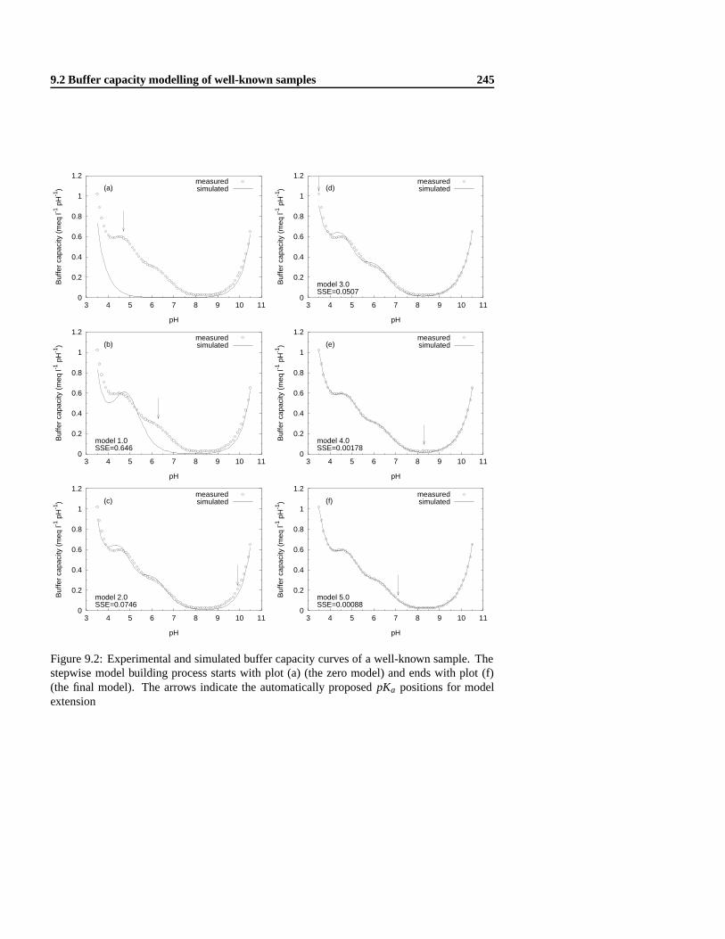
9.2 Buffer capacity modelling of well-known samples 245
0
0.2
0.4
0.6
0.8
1
1.2
3 4 5 6 7 8 9 10 11
Buf
fer
capa
city
(m
eq l-1
pH
-1)
pH
(a)measuredsimulated
0
0.2
0.4
0.6
0.8
1
1.2
3 4 5 6 7 8 9 10 11
Buf
fer
capa
city
(m
eq l-1
pH
-1)
pH
(b)
model 1.0SSE=0.646
measuredsimulated
0
0.2
0.4
0.6
0.8
1
1.2
3 4 5 6 7 8 9 10 11
Buf
fer
capa
city
(m
eq l-1
pH
-1)
pH
(c)
model 2.0SSE=0.0746
measuredsimulated
0
0.2
0.4
0.6
0.8
1
1.2
3 4 5 6 7 8 9 10 11
Buf
fer
capa
city
(m
eq l-1
pH
-1)
pH
(d)
model 3.0SSE=0.0507
measuredsimulated
0
0.2
0.4
0.6
0.8
1
1.2
3 4 5 6 7 8 9 10 11
Buf
fer
capa
city
(m
eq l-1
pH
-1)
pH
(e)
model 4.0SSE=0.00178
measuredsimulated
0
0.2
0.4
0.6
0.8
1
1.2
3 4 5 6 7 8 9 10 11
Buf
fer
capa
city
(m
eq l-1
pH
-1)
pH
(f)
model 5.0SSE=0.00088
measuredsimulated
Figure 9.2: Experimental and simulated buffer capacity curves of a well-known sample. Thestepwise model building process starts with plot (a) (the zero model) and ends with plot (f)(the final model). The arrows indicate the automatically proposed pKa positions for modelextension

246 Automatic pH buffer capacity model building
Table 9.5: Model selection criteria calculated for the consecutive models in the automaticmodel building process of the well-known testcase. The bold items mark the selected modelsbased on each considered criterion. For the last two criteria, the significance level α = 0:0001was chosen
Model 1.0 Model 2.0 Model 3.0 Model 4.0 Model 5.0 Model 6.0
AIC �330 �479 �502 �736 �782 �729AICC �256 �405 �428 �660 �705 �649FPE 0.0096 0.0012 0.00085 0.000031 0.000016 0.000035SIC �325 �470 �489 �718 �760 �701Run-test (p) < 10�6 < 10�6 0.000001 0.00013 0.00047 0.00047F-test (p) < 10�6 < 10�6 0.000003 < 10�6 < 10�6 1.00000 a
a An insignificant p-value for model 6.0 means that model 5.0 is selected.
icates entering the titration vessel through the NaOH titrant. The fourth buffer has an estimatedpKa = 3:5 and a concentration of 0.32 mmol l�1. This pKa value equals the minimum pH valueof the considered pH interval, and the model building algorithm does not allow to introducebuffers with pKa values outside the simulation interval. Therefore, the real pKa value of thatbuffer could be lower than 3.5. Its concentration indicates that this buffer is most probablythe first dissociation step of citric acid (theoretically pKa = 3:1 and 0.33 mmol l�1). The lastbuffer entered in the model is located at pH 8.21, with a very low concentration 0.02 mmol l�1.Probably, it is again a small interfering buffer, but with unknown origin. The latter buffer isnot considered very important. However, taking into account the standard deviation on the es-timate, the concentration is still significantly different from 0 (t-test, α = 0:01). As mentionedbefore, the model building process has finally tried to introduce a next buffer with pKa = 7:1(model 6.0, results not shown), but then the optimization problem became overparametrized,and the optimization algorithm failed to find an acceptable solution. Such optimization failuremostly ends up with an SSE of the current model that is higher than the SSE of the previ-ous model (which is theoretically not possible in case of correct optimization, because theless complicated model is always a subset of the more complicated model). An appropriatemessage is foreseen in the software when this happens. Further, if the optimization algorithmdoesn’ t find a correct solution, often the calculation of the variance-covariance matrix after-wards also ends up in numerical problems (e.g. Not-a-Number or NaN values). Such problemsare also logged to the user.
Although the evaluation of model selection criteria is the topic of section 9.2.3, it is usefulat this stage to summarize and interpret the different model selection criteria calculated ateach model building step for the selected testcase. More particularly, it is interesting to knowwhether the model selection criteria would stop the model building process earlier than model6.0 (which is the model that resulted in an optimization failure). The 6 model selection criteria,applied to the testcase, are summarized in Table 9.5.
If the automatic model selection was activated, all criteria would select model 5.0 as the

9.2 Buffer capacity modelling of well-known samples 247
final model, except for the Run-test, that would favour model 4.0. Of course, the latter findingcompletely depends on the choice of the critical significance level α. Also, model 6.0 endedup in a wrong optimization result, thus forcing all criteria (including the F-test) to select thesimpler model 5.0. The first four criteria (AIC, AICC, FPE and SIC) show their highest de-crease in value from model 1.0 to 2.0 and from model 3.0 to 4.0. This points to very importantincreases in model adequacy at those two stages. This is also nicely reflected in Figure 9.2. Amore detailed evaluation of the 6 model selection criteria on each of the 146 titration curves ofthe samples with well-known composition is described in section 9.2.3.
Conclusions
At this stage, a number of conclusions related to the automatic buffer capacity model buildingalgorithm can be formulated. First, the algorithm succeeds in a stepwise construction of abuffer capacity model in which the buffer systems are incorporated in order of importance.It was straightforward to relate the final result to the available a priori knowledge. Second,the results of the automatic model building revealed extra information on top of the availablea priori knowledge. More particularly, prior unknown interfering buffers at pH 8 and pH 10were detected and quantified.
Third, the standard deviations on the pKa and concentration estimates are very importantfor the interpretation. On the one hand, they are useful to statistically test if certain smallconcentrations of e.g. interfering buffers are significant; or to calculate confidence intervals onthe estimates. On the other hand, if the standard deviation becomes too high, it indicates thatthe optimization problem is overparametrized. In the testcase, the standard deviations becamesystematically lower for increasing model complexity. This strongly points to the validity ofthe more complex models. The latter conclusion was also reflected in the model selectioncriteria, that pointed to the model with 5 blind buffers as the most appropriate one. In the nextsection, the three formulated conclusions will be further evaluated with the other samples withwell-known composition.
9.2.3 Evaluation of six model selection criteria
The titration curves of the samples with well-known composition were classified in 4 groups,that are discussed separately in this section:Group 1 : 27 titration curves with 1 monoprotic buffer (oxalic acid is also considered in this
group, because of its very low pKa1 value)Group 2 : 27 titration curves with 1 di- or triprotic bufferGroup 3 : 60 titration curves with 2 buffers (mono-, di- or triprotic)Group 4 : 32 titration curves with more than 2 buffersAll titration curves were used as input data to the automatic model building environment in thesoftware bomb. It was assumed that no a priori knowledge about the buffers to be expected inthe samples was available. Consequently, the zero model only contained the water buffer. Themodel building process was repeated for each of the 6 model selection criteria. The significancelevel for the Run-test and the F-test was set to α = 0:0001.

248 Automatic pH buffer capacity model building
Summarizing frequency tables for each of the 4 groups of titration curves, with the countsof titration curves corresponding with the final (or selected) model degree 2 are given in Table9.6 for each of the 6 model selection criteria. In general, the first four criteria (AIC, AICC, PFEand SIC) select the same model as final model. However, large differences in the selected finalmodel are noticed for the Run-test and the F-test. A more detailed analysis of the selected finalmodel as function of the selected criterion, and for each of the 4 considered groups of titrationcurves is given in the next paragraphs.
In group 1, the automatic model building algorithm perfectly detects the single monoproticbuffer in the experimental buffer capacity profile, and in all cases incorporates this buffer as thefirst blind buffer in the model. The estimated concentrations were not significantly differentfrom the theoretically expected concentrations. However, the model building process does notstop at this stage in most cases, but continues with the incorporation of new blind buffers. Inorder of importance, first a buffer around pH 10 with a typical concentration of 0.1 mmol l�1,and second a buffer around pH 6.5 with a typical concentration between 0.05 and 0.1 mmol l�1
are added to the model. As discussed before, these two buffers are assumed to be silicate andinorganic carbon respectively. Their concentrations are mostly found significantly differentfrom 0. The Run-test and F-test generally stop at this stage. However, the AIC and relatedcriteria mostly extend the model with 1 or even 2 extra buffers of unknown origin (aroundpH 7 and pH 4). The concentrations of these extra buffers are very low, and sometimes notsignificantly different from 0. Practically, it is concluded that the AIC and related criteria gorather far in the model building process. In 7 out of the 27 cases, the F-test selected the modelwith only 1 buffer as the final model, thus not recognizing the silicate and/or the IC buffer.This behaviour could be attributed to an optimization problem. It was noticed that for some‘uncomplete’ models (thus models still deviating a lot from the final model), the parameterestimation routine ended in a local minimum (5 cases out of the 27) at the second modellingstep, i.e. the model with 2 blind buffers, with an SSE of the more complex model higher thanthe SSE of the simpler model. Consequently, the simpler model was selected by the F-test.The AIC and related criteria too suffered from this flaw, and as a result selected in 4 (AIC,AICC and FPE) or 5 (SIC) cases the model with 1 buffer as the final model. Only the Run-testwas not influenced by local minima problems, because this test examines only the randomnessof the residuals. As a first preliminary conclusion, the Run-test was found to perform most‘ realistically’ for this group of titration curves.
For the titration curves of group 2, similar findings as for group 1 can be formulated.The final models mostly contain, as expected, 1 or 2 supplementary buffers compared to thefinals models of group 1. For example, in 17 out of 27 cases, the Run-test selects the modelwith 4 blind buffers. These 4 buffers include 2 or 3 buffers from the added di- or triproticcomponent, and 1 or 2 interfering buffers, like silicates or IC. The AIC and related criteriaoften select a model with 5 or 6 blind buffers. This is again a higher model degree thanwhat should be considered practically. Further, these high degree models illustrate certainweaknesses in the model building algorithm. More particularly, sometimes buffers are added inthe model (interfering buffers, in small but significant concentrations), that in a later modellingstage become insignificant, because a neighbouring buffer takes over the buffer capacity of thepreviously introduced buffer. The model building algorithm does not allow to remove a buffer
2The degree of a model is here defined as the number of blind buffers incorporated in the model.

9.2 Buffer capacity modelling of well-known samples 249
Table 9.6: Frequency tables per group of titration curves, classified towards the final modeldegree and the applied model selection criterion
Group Final model Criterion for model selection
degree AIC AICC FPE SIC Run-test F-test
1 1 4 4 4 5 1 71 2 2 2 2 4 7 51 3 2 2 2 4 19 91 4 14 14 14 11 0 61 5 5 5 5 3 0 0
2 1 1 1 1 1 0 42 2 0 0 0 2 0 102 3 1 1 1 2 5 22 4 7 7 7 7 17 22 5 11 11 11 9 5 62 6 7 7 7 6 0 3
3 1 0 0 0 0 0 33 2 0 0 0 1 1 53 3 2 2 2 2 14 13 4 13 13 13 16 19 233 5 36 36 36 34 17 263 6 9 9 9 7 3 23 7 0 0 0 0 0 03 8 0 0 0 0 6 0
4 3 0 0 0 0 1 04 4 3 3 3 3 7 64 5 9 9 9 10 16 104 6 16 16 16 15 8 164 7 4 4 4 4 0 0

250 Automatic pH buffer capacity model building
from the model in case the concentration of this buffer is not significantly different from 0.It could be suggested to include this feature in the model building algorithm of the softwarebomb(e.g. based on a similar F-test based method that is also implemented in stepwise linearregression algorithms). This is further discussed in section 9.2.4. Local minima problemswith ‘uncomplete models’ , as described earlier, did occur less frequently (only 1 out of the 27cases). In groups 3 and 4, this particular problem was no longer noticed. Thus it is concludedthat only the simplest type of titration curves sometimes lead to a too low final model degreedue to an optimization problem. Again, the Run-test was found to select the most realistic finalmodel.
The titration curves of group 3 have an increased complexity, and should theoreticallycontain at least between 2 (e.g. amm�ace) and 5 (e.g. cit�mal) pKa values. For the simplesttype of combinations (e.g. the combination of a monoprotic and a diprotic buffer), the finalmodel could be interpreted perfectly: The quantified buffers corresponded with the bufferspresent, both for the pKa positions, and the respective concentrations. Again, supplementarybuffers were sometimes found around pH 10 (silicates) or elsewhere. A typical example ofone of these titration curves was described earlier in section 9.2.2. At this stage, anotherparticularity related to the model building algorithm was discovered. In the example cit�mal,the pKa2 = 5:69 of malonic acid is only 0.7 different from the pKa3 = 6:39 of citric acid. Inmost examples of this type, a blind buffer was incorporated in the model somewhere betweenthese 2 theoretical pKa values, and was accounting for both buffer systems. This points to acertain ‘ limit of resolution’ which is further discussed in the next paragraph. For the simplesttype of curves in group 3, the Run-test was slightly favoured for practical purposes. However,for the more complicated titration curves, the performance of the Run-test was not found mostappropriate in a number of situations. More particularly, for 6 out of 60 titration curves, theRun-test selected a final model with 8 blind buffers, whereas all other criteria considered only6 blind buffers as the maximum number of buffers needed in the final model. There is aclear explanation for this behaviour. The maximum number of buffers that are available inthe automatic model building algorithm is 8. Therefore, in those cases where the Run-testselected 8 blind buffers, the necessary Run-test criterion was never reached. This phenomenonoccurred only in examples with polyphosphate as one of the buffers. It can be pointed that theuncertain position of the pKa2 value of polyphosphate could be the reason why an acceptablefit was not found with the Run-test criterion. By lowering the significance level α, this problemwould partially be solved. However, this is an important limitation for field applications. Anillustrative titration example of pho�mal is given in Figure 9.3. The fitted buffer capacitymodel contains 4 blind buffers (with respectively the pKa values in order of importance 5.7,9.3, 3.5 and 6.8). A further model extension proposed at pH 8.1 results in an insignificantF-test result (p= 0:26), whereas the Run-test result is still very significant (u= �4:5 or p=0:000007). Further model extensions do not make the fit better than what is illustrated inFigure 9.3. When 6 or more blind buffers are included in the model, the optimization problembecomes overparametrized, and the parameter estimation algorithm ends up in local minima.Thus, when the Run-test criterion is selected for this particular example (with α = 0:0001), themodel building algorithm will proceed until all available blind buffers are incorporated in themodel, and will finally not find any model that fulfils the requested criterion.
The final model results of the easiest type of titration curves in group 4 (e.g. the combina-tion of 2 monoprotic buffers and a diprotic buffer) could easily be related with the buffers to be

9.2 Buffer capacity modelling of well-known samples 251
0
0.2
0.4
0.6
0.8
1
1.2
3 4 5 6 7 8 9 10 11
Buf
fer
capa
city
(m
eq l-1
pH
-1)
pH
(a)
SSE=0.00150model 4.0
measuredsimulated
-0.1
-0.05
0
0.05
0.1
3 4 5 6 7 8 9 10 11
Res
idua
ls (
meq
l-1 p
H-1
)pH
(b)
Figure 9.3: Experimental and simulated buffer capacity curves (a) and calculated residuals (b)of a sample pho�mal
expected. The F-test criterion mostly selected the same model as the AIC and related criteria.The Run-test criterion often selected models of lower complexity. The results obtained withthe F-test criterion were found to correspond most closely to the reality. The interfering bufferat pH 10 (silicates) was still detected and quantified in most cases. The ‘ limit of resolution’mentioned in the previous paragraph, was further investigated. Again, it was found that 2buffers with neighbouring pKa values are pooled together in the model building algorithm. Itwas found that the practical limit of resolution for the considered examples is between 0.5 and1 pH units. This can be related with two parameter settings of the model building algorithm(see chapter 5): The initial range 3 of a blind pKa value is chosen 1.5, and the minimal range ofa blind pKa value is set to 0.2. The intervals of the pKa values are not allowed to overlap, thusthis automatically limits the number of buffers that can enter in the model around the samepKa. However, detailed analysis of the pKa ranges that were automatically narrowed duringthe model building process showed that only in a few cases, the minimal range was used bythe algorithm. This indicates that the model building algorithm did not request to enter newblind buffers with a pKa separation of 0.5 or less compared to pKa values of previously incor-porated buffers in the model. A comparison with the Gordon algorithm described in [101, 102]was made, and the defined criterion for the limit of resolution (see equation (4.5) on page 92)was compared with the obtained results. The authors found that a minimal pKa separationof 0.1�0.2 is borderline for most applications, whereas 0.5 is a common value. However, itshould be noted that the Gordon algorithm only allows variation on the pKa value that is lastlyentered in the model, together with the neighbouring pKa value, whereas in the bombalgo-rithm, variation may be allowed on any pKa. As mentioned and illustrated in section 4.4.2 onpage 89, such approach is only useful under well controlled laboratory conditions. It can beconcluded that the limit of resolution obtained here is somewhat lower than what is described
3The range is defined as the difference between the maximum and minimum boundary value set as an interval inwhich the considered pKa value is allowed to vary.
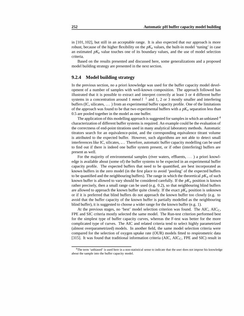
252 Automatic pH buffer capacity model building
in [101, 102], but still in an acceptable range. It is also expected that our approach is morerobust, because of the higher flexibility on the pKa values, the built-in model ‘ tuning’ in casean estimated pKa value touches one of its boundary values, and the use of model selectioncriteria.
Based on the results presented and discussed here, some generalizations and a proposedmodel building strategy are presented in the next section.
9.2.4 Model building strategy
In the previous section, no a priori knowledge was used for the buffer capacity model devel-opment of a number of samples with well-known composition. The approach followed hasillustrated that it is possible to extract and interpret correctly at least 3 or 4 different buffersystems in a concentration around 1 mmol l�1 and 1, 2 or 3 mostly smaller and interferingbuffers (IC, silicates, : : : ) from an experimental buffer capacity profile. One of the limitationsof the approach was found to be that two experimental buffers with a pKa separation less than0.5 are pooled together in the model as one buffer.
The application of this modelling approach is suggested for samples in which an unbiased 4
characterization of different buffer systems is required. An example could be the evaluation ofthe correctness of end-point titrations used in many analytical laboratory methods. Automatictitrators search for an equivalence-point, and the corresponding equivalence titrant volumeis attributed to the expected buffer. However, such algorithms are not able to detect smallinterferences like IC, silicates, : : : Therefore, automatic buffer capacity modelling can be usedto find out if there is indeed one buffer system present, or if other (interfering) buffers arepresent as well.
For the majority of environmental samples (river waters, effluents, : : : ) a priori knowl-edge is available about (some of) the buffer systems to be expected in an experimental buffercapacity profile. The expected buffers that need to be quantified, are best incorporated asknown buffers in the zero model (in the first place to avoid ‘pooling’ of the expected buffersto be quantified and the neighbouring buffers). The range in which the theoretical pKa of suchknown buffer is allowed to vary should be considered carefully. If the pKa position is knownrather precisely, then a small range can be used (e.g. 0.2), so that neighbouring blind buffersare allowed to approach the known buffer quite closely. If the exact pKa position is unknownor if it is preferred that blind buffers do not approach the known buffer too closely (e.g. toavoid that the buffer capacity of the known buffer is partially modelled as the neighbouringblind buffer), it is suggested to choose a wider range for the known buffer (e.g. 1).
At the previous stages, no ‘best’ model selection criterion was found. The AIC, AICC,FPE and SIC criteria mostly selected the same model. The Run-test criterion performed bestfor the simplest type of buffer capacity curves, whereas the F-test was better for the morecomplicated type of curves. The AIC and related criteria tend to select highly parametrized(almost overparametrized) models. In another field, the same model selection criteria werecompared for the selection of oxygen uptake rate (OUR) models fitted to respirometric data[315]. It was found that traditional information criteria (AIC, AICC, FPE and SIC) result in
4The term ‘unbiased’ is used here in a non-statistical sense to indicate that the user does not impose his knowledgeabout the sample into the buffer capacity model.

9.2 Buffer capacity modelling of well-known samples 253
overfitting of the model compared to the ‘human expert advice’ . In particular, some smalloscillations in the data were accounted for to a significant extent by flexible, more complexmodels. To the human expert, however, these phenomena seemed not essential [315]. Thelatter statement also applies to the results obtained in this work. In the next sections, onlythree model selection criteria will further be considered and evaluated, being AIC, Run-testand F-test.
If the F-test criterion is selected, an useful comparison can be made with multiple linearregression search procedures for the selection of independent variables in a multiple linearregression model. There is, however, a fundamental difference in approach between the au-tomatic buffer capacity model building procedure and multiple linear regression. In linearregression problems, the independent or exploratory variables Xi are known in advance, and asubset from the pool of a priori known Xi variables is included in the final or ‘best’ regressionmodel. With the buffer capacity model building algorithm, the buffers that are entered in themodel (cfr. the Xi) are not a priori known, but determined as function of the residual pattern ofthe previous model. The different procedures for multiple linear regression [207] are shortlyreviewed and discussed in relation with stepwise buffer capacity modelling.
� All-possible-regressions: This procedure calls for considering all possible subsets ofthe pool of potential Xi variables and identifies for detailed examination a few ‘good’subsets according to some criterion. For example with 4 exploratory variables, there arealtogether 16 subset regression models that can be formed. First, there is the regressionmodel with no Xi variables, then with one Xi variable, with two Xi variables, etc. Due tothe fundamental difference mentioned above, such approach would not be feasible forautomatic buffer capacity modelling.
� Forward stepwise regression: Essentially, this search method develops a sequence of re-gression models, at each step adding or deleting an Xi variable. It is probably the mostwidely used method and it was developed to economize on computational efforts, ascompared with the all-possible-regressions procedure. The criterion for adding or delet-ing an Xi variable is mostly an F-test. Further, two critical significance levels need tobe chosen: a minimum significance level to enter, and a maximum significance level toremove. Note that the stepwise regression algorithm allows an Xi variable, brought inthe model at an earlier stage, to be dropped subsequently if it is no longer helpful inconjunction with variables added at later stages. The current algorithm in bombdoesnot allow to remove buffers from the buffer capacity model once they are incorporated.However, as described in section 9.2.3, it happens that the concentration of a buffer in-troduced at an earlier stage becomes insignificant at later stages. Consequently, an usefulextension of the current algorithm would be to allow the removal of insignificant buffersfrom the model. On the other hand, this would make the algorithm more complicated,and certainly would require extra research to make it robust enough for field-use.
� Forward selection: This search method is a simplified version of forward stepwise re-gression, omitting the test whether a variable once entered into the model should bedropped. This corresponds best with the current algorithm in the program bomb.
� Backward elimination: The backward elimination search procedure is the opposite offorward selection. It begins with the model containing all potential Xi variables andidentifies the one with the smallest F-test value. If the significance of this value exceeds

254 Automatic pH buffer capacity model building
a maximum significance level to remove, that Xi variable is dropped. Such procedureis not foreseen in the current version of bomb, however, it should be possible in furtherresearch to extend the algorithm with a backward elimination method. Because theelimination method is simpler than the stepwise method mentioned above, it is expectedthat the robustness of the new algorithm would be similar as the current algorithm. Somestatisticians argue for backward methods over forward methods because it is useful as afirst step to look at each Xi in the regression function adjusted for all the other Xi variablesin the pool [207]. For buffer capacity modelling purposes, a backward algorithm wouldnot suffer from a particular problem described in section 9.2.3, being the selection ofa too low degree model caused by local minima problems in still very ‘uncomplete’models.
9.3 Surface water and effluent applications
9.3.1 Materials and methods
The titration curves that were used for the evaluation of the automatic buffer capacity modellingare described earlier in chapter 6, more particularly in section 6.3.3 on page 151. Summarized,421 titration curves were analyzed, originating from
� domestic wastewater effluents (26 different plants),� an industrial effluent sampled during three months, and� 118 Flemish surface waters.
The a priori knowledge that holds for all titration curves is that an ortho-phosphate buffer,an ammonium buffer and an IC buffer are to be expected. As discussed in section 9.2.4,it is considered important to use such a priori knowledge in the automatic buffer capacitymodel development. Therefore, the zero model or starting model is chosen in correspondencewith the model specifications given in Table 6.3 on page 152, except for the following twomodifications:
� The ‘soap’ buffer is not included any more. The automatic modelling algorithm hasnow the flexibility to include no, one, two or more buffer systems that account for thepreviously used ‘soap’ buffer between pH 4 and pH 6.
� The simulation interval (between pH 4 and pH 10 in the work presented in chapter 6)is now extended to an interval between pH 3.5 and pH 10.5. This offers the possibilityto take into account more potentially present buffer systems. A further extension of thesimulation interval is not advised, for two reasons. First, outside the above mentionedinterval, the water buffer capacity is masking all other buffers, and thus it is not worth-while to search for extra buffers with such low or high pKa values. Second, it was foundthat the optimization algorithm easily ends up in local minima when the simulation inter-val is set very wide, e.g. between pH 3 and pH 11. The most probable reason is that thebuffer capacities at pH 3 and pH 11 are approximately ten times higher than the buffercapacities at pH 5�7. Therefore, the optimization algorithm will focus too much on thegoodness of fit at the lowest and highest pH values, and neglect the goodness of fit in thecentral part of the buffer capacity profile, which is undoubtedly the most important part

9.3 Surface water and effluent applications 255
of the profile. For future versions of the program bomb, it is suggested to implement arelative weighing option in the cost function to overcome this problem. More particu-larly, it is proposed to use a high cost function weight in the low buffer capacity regions,and vice versa.
Based on the above described zero model, the automatic model building algorithm maystepwise enter blind buffers in the model, but not with pKa’s in the 2 pH ranges 6:5� 7:4and 9�9:75, which are the lower and upper limits for the variable pKa values of respectivelyortho-phosphate and ammonium. Other important settings for the automatic model buildingalgorithm in bombare: α = 0:0001 as the critical significance level for the Run-test and F-test,and 0.2 as the minimal range for a pKa of a blind buffer. In section 9.2.3, it was found that theAIC, AICC, FPE and SIC model selection criteria performed very similar. Therefore, in thissection, only AIC, Run-test and F-test will be evaluated and compared with each other.
In the next section, the following points will be investigated:
� What are the differences in the final model results when considering the different modelselection criteria?
� Is the automatic model building algorithm able to detect and quantify other buffers thanammonium and ortho-phosphate, and does this reveal extra information about the titratedsample?
� Is the automatic model building advantageous for ammonium and ortho-phosphate as-sessment, compared to the fixed model approach that was used in chapter 6?
9.3.2 Automatic model building results
Evaluation of three model selection criteria
Summarizing frequency tables for the surface waters (259 titration curves) and effluents (162titration curves), with the counts of titration curves corresponding with the final model degreefor each of the three model selection criteria are given in Table 9.7.
For most surface waters and effluent samples, the three model selection gave satisfyingresults. A strict comparison between the ‘selected’ model degree and the ‘ real’ model degree isnot possible, because the ‘ real’ model degree is unknown, and differs from sample to sample.Therefore, an ‘expert judgement’ was needed for each titrated sample. The AIC criterionagain tends to select higher degree models. Two typical problems were noticed. First, theRun-test criterion is not reached in 33 % of the cases, resulting in a final model in which themaximum allowable (6) blind buffers are entered in the model, whereas the other criteria haveselected a final model of lower degree. In most of these cases, the optimization algorithmends up in local minima and the variance-covariance calculation is not correctly finished dueto numerical problems. This is a serious limitation for field-use, and thus the Run-test criterionas such is found not very robust. Second, in 20 % of the cases the F-test criterion concludesthat model 1.x (zero model plus 1 blind buffer) is not significantly different from model 0.0(zero model), and therefore selects the zero model as the final model. Visual inspection of theexperimental versus the simulated buffer capacity curve shows in most of these cases that thereis still unmodelled experimental buffer capacity, and thus the F-test has selected a final modelwith a too low degree. Moreover, when the further model building steps (e.g. model 2.x or

256 Automatic pH buffer capacity model building
Table 9.7: Frequency tables of surface water and effluent samples, classified towards the finalmodel degree and the applied model selection criterion
Final model 259 surface water samples 162 effluent samples
degree AIC Run-test F-test AIC Run-test F-test
0 14 0 41 2 3 441 28 4 93 15 8 532 49 10 71 36 15 343 116 61 38 64 38 224 47 55 15 40 22 95 5 40 1 5 25 06 0 89 0 0 51 0
3.x) are performed anyway, it can happen that the F-test criterion again becomes significant forthese higher degree models. The origin of this problem can be found in the way the automaticmodel building algorithm proceeds, i.e. the algorithm can only introduce one blind buffer at atime. If the model fit of the zero model is bad at several positions of the buffer capacity profile,then the algorithm can increase the fit at only one position of the profile. Consequently, it ispossible that such a ‘small’ increase in fit by adding one blind buffer is not significant dueto lack of fit of the other positions in the buffer capacity profile, despite that a blind buffer isalways introduced at the pKa position that suits best for a model extension. 5 This particularproblem automatically disappears for more complicated models with several blind buffers.Note that the backward elimination suggestion formulated in section 9.2.4 would automaticallysolve this problem.
From this analysis, it can be concluded that the three model selection criteria have a clearlydifferent behaviour. At this moment, none of the three criteria can be proposed as the ‘best’criterion, which was also concluded in section 9.2.4. In the next paragraphs, a number ofcase studies will be presented in detail for further evaluation and interpretation of the modelselection criteria and their corresponding final models.
Surface waters
Four selected Flemish surface waters samples, that were introduced and discussed earlier (seeTable 6.4 on page 161 and Figure 6.13 on page 160), are reconsidered for detailed analysisof the automatic model building results. Summarized results are presented in Table 9.8, andthe corresponding graphs are shown in Figures 9.4, 9.5, 9.6 and 9.7. Note that the standarddeviations of the concentration estimates are calculated with the Nelder and Mead method (seesection 5.3.3 on page 120), and not from replicate samples.
The first case, shown in Figure 9.4, illustrates the two above mentioned problems with
5How this pKa position for model extension is determined is illustrated in Figure 5.16 on page 128.

9.3 Surface water and effluent applications 257
0
0.2
0.4
0.6
0.8
1
1.2
1.4
3 4 5 6 7 8 9 10 11
Buf
fer
capa
city
(m
eq l-1
pH
-1)
pH
(a)final model, F-test
model 0.0SSE=0.09943
measuredsimulated
0
0.2
0.4
0.6
0.8
1
1.2
1.4
3 4 5 6 7 8 9 10 11
Buf
fer
capa
city
(m
eq l-1
pH
-1)
pH
(b)
model 1.1SSE=0.09339
measuredsimulated
0
0.2
0.4
0.6
0.8
1
1.2
1.4
3 4 5 6 7 8 9 10 11
Buf
fer
capa
city
(m
eq l-1
pH
-1)
pH
(c)final model, AIC
model 2.0SSE=0.01947
measuredsimulated
0
0.2
0.4
0.6
0.8
1
1.2
1.4
3 4 5 6 7 8 9 10 11
Buf
fer
capa
city
(m
eq l-1
pH
-1)
pH
(d)
model 3.2SSE=0.01939
measuredsimulated
Figure 9.4: Experimental and simulated buffer capacity curves of the surface water BassinSmedenstraat, Roeselare. The stepwise model building process starts with plot (a) (the zeromodel) and ends with plot (d). The final model for each model selection criterion is indi-cated on the graph. The arrows indicate the automatically proposed pKa positions for modelextension
258 Automatic pH buffer capacity model building
0
0.5
1
1.5
2
2.5
3
3.5
3 4 5 6 7 8 9 10 11
Buf
fer
capa
city
(m
eq l-1
pH
-1)
pH
(a)
model 0.0SSE=0.29447
measuredsimulated
0
0.5
1
1.5
2
2.5
3
3.5
3 4 5 6 7 8 9 10 11
Buf
fer
capa
city
(m
eq l-1
pH
-1)
pH
(b)final model, F-test
model 1.1SSE=0.18912
measuredsimulated
0
0.5
1
1.5
2
2.5
3
3.5
3 4 5 6 7 8 9 10 11
Buf
fer
capa
city
(m
eq l-1
pH
-1)
pH
(c)
model 2.2SSE=0.14525
measuredsimulated
0
0.5
1
1.5
2
2.5
3
3.5
3 4 5 6 7 8 9 10 11
Buf
fer
capa
city
(m
eq l-1
pH
-1)
pH
(d)
model 3.2SSE=0.07486
measuredsimulated
0
0.5
1
1.5
2
2.5
3
3.5
3 4 5 6 7 8 9 10 11
Buf
fer
capa
city
(m
eq l-1
pH
-1)
pH
(e)final model, AIC & Run-test
model 4.1SSE=0.06821
measuredsimulated
Figure 9.5: Experimental and simulated buffer capacity curves of the surface water Vuile beek,Ieper. The stepwise model building process starts with plot (a) (the zero model) and ends withplot (e). The final model for each model selection criterion is indicated on the graph. Thearrows indicate the automatically proposed pKa positions for model extension

9.3 Surface water and effluent applications 259
0
0.2
0.4
0.6
0.8
1
3 4 5 6 7 8 9 10 11
Buf
fer
capa
city
(m
eq l-1
pH
-1)
pH
(a)model 0.0
SSE=0.04928measuredsimulated
0
0.2
0.4
0.6
0.8
1
3 4 5 6 7 8 9 10 11
Buf
fer
capa
city
(m
eq l-1
pH
-1)
pH
(b)final model, Run-test
model 1.0SSE=0.00354
measuredsimulated
0
0.2
0.4
0.6
0.8
1
3 4 5 6 7 8 9 10 11
Buf
fer
capa
city
(m
eq l-1
pH
-1)
pH
(c)final model, F-test
model 2.0SSE=0.00194
measuredsimulated
0
0.2
0.4
0.6
0.8
1
3 4 5 6 7 8 9 10 11
Buf
fer
capa
city
(m
eq l-1
pH
-1)
pH
(d)final model, AIC
model 3.1SSE=0.00176
measuredsimulated
Figure 9.6: Experimental and simulated buffer capacity curves of the surface water Scherpen-bergbeek, Poperinge. The stepwise model building process starts with plot (a) (the zero model)and ends with plot (d). The final model for each model selection criterion is indicated on thegraph. The arrows indicate the automatically proposed pKa positions for model extension

260 Automatic pH buffer capacity model building
0
0.2
0.4
0.6
0.8
1
1.2
3 4 5 6 7 8 9 10 11
Buf
fer
capa
city
(m
eq l-1
pH
-1)
pH
(a)
model 0.0SSE=0.30947
measuredsimulated
0
0.2
0.4
0.6
0.8
1
1.2
3 4 5 6 7 8 9 10 11
Buf
fer
capa
city
(m
eq l-1
pH
-1)
pH
(b)
model 1.2SSE=0.12672
measuredsimulated
0
0.2
0.4
0.6
0.8
1
1.2
3 4 5 6 7 8 9 10 11
Buf
fer
capa
city
(m
eq l-1
pH
-1)
pH
(c)final model, F-test
model 2.2SSE=0.08831
measuredsimulated
0
0.2
0.4
0.6
0.8
1
1.2
3 4 5 6 7 8 9 10 11
Buf
fer
capa
city
(m
eq l-1
pH
-1)
pH
(d)
model 3.0SSE=0.07221
measuredsimulated
0
0.2
0.4
0.6
0.8
1
1.2
3 4 5 6 7 8 9 10 11
Buf
fer
capa
city
(m
eq l-1
pH
-1)
pH
(e)final model, AIC
model 4.1SSE=0.00882
measuredsimulated
0
0.2
0.4
0.6
0.8
1
1.2
3 4 5 6 7 8 9 10 11
Buf
fer
capa
city
(m
eq l-1
pH
-1)
pH
(f)final model, Run-test
model 5.1SSE=0.00792
measuredsimulated
Figure 9.7: Experimental and simulated buffer capacity curves of the surface water Zarrenbeek,Staden. The stepwise model building process starts with plot (a) (the zero model) and endswith plot (f). The final model for each model selection criterion is indicated on the graph. Thearrows indicate the automatically proposed pKa positions for model extension

9.3 Surface water and effluent applications 261
Table 9.8: Ammonium and ortho-phosphate model building results for 4 selected Flemishsurface waters, compared with results previously described in chapter 6. The concentrationsare expressed as mgN l�1 or mgP l�1 and the table entries are estimate � standard deviation
Automatic model building results Results of chapter 6
Buffer Figure AIC Run-test F-test laboratorya AQMON Figure
NH+4 9.4 17:8�0:61 � 19:7�0:48 10:9�1:63 19:3�0:12 6.13(a)NH+4 9.5 72:7�1:54 72:7�1:54 77:3�0:77 62:0�4:81 76:7�0:68 6.13(b)NH+4 9.6 1:08�1:20 1:15�0:07 1:32�0:08 0:33�0:06 1:22�0:04 6.13(e)NH+4 9.7 6:29�0:44 6:34�0:37 9:82�0:79 2:80�0:28 8:98�0:40 6.13(f)
o-PO4 9.4 4:03�3:67 � 2:68�0:91 2:60�0:57 2:36�0:30 6.13(a)o-PO4 9.5 8:65�2:89 8:65�2:89 8:17�2:10 8:45�0:35 7:73�2:13 6.13(b)o-PO4 9.6 0:70�0:35 0:48�0:18 0:79�0:13 0:19�0:04 0:62�0:08 6.13(e)o-PO4 9.7 4:84�1:06 4:19�0:93 6:52�0:96 3:25�0:64 6:17�0:60 6.13(f)
a Mean and standard deviation of the laboratory A and B results in Table 6.4 on page 161.
respectively the F-test and the Run-test. The F-test selects the zero-model as the final model,although there is a clear extra buffer present at pH 4.5 (estimated in further models as a sig-nificant concentration of 0.05 mmol l�1). The second problem is the Run-test criterion, whichwas never fulfilled in this case. For models 1.x, 2.x and 3.x the test statistic for the Run-test isstill very significant (u= �4:5 or p= 0:000007), and becomes even more significant for thehigher degree models (theoretically this is not possible, however as described earlier, optimiza-tion problems are the origin of this behaviour). The AIC criterion selects model 2.0, which isprobably the best choice. A comparison of the titrimetric ammonium and ortho-phosphate es-timations with the laboratory analysis (see Table 9.8) does not clearly indicate which modelselection criterion gave the best estimations of N and P. The incorporation of an extra bufferat pH 10.5 has a positive influence on the estimated concentration of ammonium. However,the ortho-phosphate concentration estimated with model 2.0 is less reliable (very high stan-dard deviation) and less accurate than the estimate with model 0.0. Even in the model withthe highest degree, i.e. model 3.2 in Figure 9.4(d), still a visible lack of fit between pH 9 andpH 10 is noticed. This is caused by the ammonium buffer in the model, which is not perfectlyfitted, together with the restriction that the model building algorithm may not introduce blindbuffers at the pKa positions reserved for known buffers, like ammonium.
In the second example, illustrated in Figure 9.5, the F-test selects model 1.1. This is anacceptable result, because the model fit for model 2.2 is only slightly better than model 1.1.The AIC and Run-test criterion select the model with 4 blind buffers as the final model. Thetwo blind buffers at pH 8.9 and 10.2 make that the ammonium estimation is around 5 mgN l �1
lower than in e.g. model 1.1. In this particular case, this has as a result that the ammoniumestimation is closer to the laboratory value for model 4.1 compared to the result for model1.1. The estimated ortho-phosphate concentrations differ only slightly when comparing theconsecutive fitted models.

262 Automatic pH buffer capacity model building
The third selected sample, shown in Figure 9.6, is an example of a clean surface water, withlaboratory concentrations of N and P far below 1 mg l�1. The F-test and AIC criterion selectmodel 2.0 and model 3.1 respectively, which can be considered realistic models. However, theRun-test criterion selects model 1.0, which, from a practical point of view, is a model of too lowdegree. Earlier interpretations (see e.g. Figure 6.13(e)) have illustrated that at least two buffersare present in the pH range lower than 6. With the AIC and F-test criteria, two buffers in thatrange are detected, with pKa’s respectively equal to 3.5 and 5.3. The behaviour of the Run-testcriterion in this example is rather exceptional, because the Run-test more often selects modelsof too high degree (or the criterion is never reached). The final estimated concentrations ofN and P are slightly influenced by the automatically built models compared to the previouslyobtained AQMON results.
The last selected sample, illustrated in Figure 9.7, was earlier described as the most extremeexample for which the previously obtained model fit was unacceptable (see Figure 6.13(f)).Therefore, the earlier estimated concentrations of N and P could not be trusted. The automati-cally built models need at least 4 blind buffers for a reasonable model fit. This time, the F-testcriterion fails because it selects a model of too low degree. The AIC and Run-test criteria se-lect respectively model 4.1 and model 5.1, which are both considered realistic models. The Nand P concentrations estimated with the latter two mentioned models are more closely to thelaboratory data compared to the previously obtained AQMON results. This clearly illustratesthe advantage of the automatic model building in this particular case.
At the current stage, for samples of the type ‘surface water’ , it might be concluded that theAIC criterion is superior to the Run-test and F-test criterion. Although the AIC criterion some-times tends to select high degree models, it does not suffer from the two major disadvantagesof respectively the Run-test (i.e. that the criterion sometimes never fulfils) and the F-test (i.e.the selection of a too low degree model).
The ammonium and ortho-phosphate estimations resulting from automatically built buffercapacity models based on the AIC selection criterion were compared with the laboratory de-termined concentrations. This was performed for the 118 Flemish surface waters, similarly towhat is illustrated in Figure 6.11 on page 158. The only but important difference is that theresults of chapter 6 were obtained with a fixed buffer capacity model, whereas in this chapter,the results are derived from automatically built models, custom-made for each individual sam-ple. Despite the significantly better results for a number of individual samples (see also someof the selected samples above) with the automatic modelling approach, the overall comparisonbetween laboratory and titrimetric results via scatterplots was only slightly different from theresults described in chapter 6 (results not shown). In about 5 % of the samples, it was foundthat the automatically built final model did not fit sufficiently to the experimental data, due tothe selection of a model with a too low degree. This problem was already described in section9.2.3 and originates from a local minimum problem of the parameter estimation algorithm.Fortunately, the problem is well-defined, and a suggestion for an alternative algorithm (back-ward elimination) that doesn’ t suffer from this shortcoming was formulated in section 9.2.4.Also the Run-test is a reasonable alternative for these problematic cases.

9.3 Surface water and effluent applications 263
Table 9.9: Ammonium and ortho-phosphate model building results for 3 selected effluent sam-ples, compared with prior obtained results in chapter 6. The concentrations are expressed asmgN l�1 or mgP l�1 and the table entries are estimate � standard deviation
Automatic model building results Previously obtained results
Buffer Figure AIC laboratory a AQMON
NH+4 9.8(a1)�(a2) 10:8�0:42 5:89�0:02 14:9�0:19
NH+4 9.8(b1)�(b2) 17:0�0:82 16:4�3:68 23:1�0:60
NH+4 9.8(c1)�(c2) 4:87�0:94 2.03 b 8:03�0:33
o-PO4 9.8(a1)�(a2) 2:89�2:38 1:79�0:02 2:36�0:30o-PO4 9.8(b1)�(b2) 5:95�7:07 5:75�2:62 9:43�1:41o-PO4 9.8(c1)�(c2) 6:43�4:79 6:55�1:06 14:7�0:87a Mean and standard deviation of the laboratory A and B results.b There is only 1 laboratory result.
Effluents
The automatic buffer capacity model building of effluent samples gives results similar to thesurface waters. However, some new interesting phenomena were observed for the industrialeffluent samples. One domestic wastewater effluent (Hofstade, sampled at October 19, 1993)and two industrial effluent samples (sampled respectively at April 20 and 27, 1994) are selectedfor more detailed analysis and discussion. The summarized results of the selected samples aregiven in Table 9.9, and the corresponding graphs are shown in Figure 9.8.
The first example, illustrated in Figure 9.8(a) is a typical case of buffers interfering withthe ammonium estimation. Without automatic model building, the estimated ammonium con-centration was about three times higher than the measured laboratory concentration. Withautomatic model building, two interfering buffers at pH 9 and 10.5 of respectively 0.1 and 0.6mmol l�1 are recognized. As a consequence, the ammonium estimation becomes lower thanbefore, but the estimation is still almost two times higher than the laboratory concentration.This indicates that other interferences could be present at the same pKa as ammonium. Nointerfering buffers around the ortho-phosphate pKa2 are found, and, thus the estimated ortho-phosphate concentration is not significantly different compared to the previously obtained re-sults. The standard deviations on the estimates of ortho-phosphate are rather high, indicatinga high uncertainty of the estimated values. The presence of the IC buffer and blind buffers inthe neighbourhood of the ortho-phosphate buffer is pointed to as a reason for this.
The second and third example represent industrial effluent samples that were both taken inthe third month of the measurement period. As mentioned in section 6.3.3 on page 151, thewastewater treatment plant was in a start-up phase, with very high ammonium concentrations(> 200 mgN l�1) in the first two months and lower concentrations (< 20 mgN l�1) in the lastmonth of the measurement period. For the samples taken in the first two months, the fixedmodel approach (chapter 6) resulted already in an acceptable agreement between the exper-

264 Automatic pH buffer capacity model building
0
0.2
0.4
0.6
0.8
1
1.2
1.4
3 4 5 6 7 8 9 10 11
Buf
fer
capa
city
(m
eq l-1
pH
-1)
pH
(a1)
model 0.0SSE=0.13789
measuredsimulated
0
0.2
0.4
0.6
0.8
1
1.2
1.4
1.6
1.8
3 4 5 6 7 8 9 10 11
Buf
fer
capa
city
(m
eq l-1
pH
-1)
pH
(b1)
model 0.0SSE=1.21018
measuredsimulated
0
0.2
0.4
0.6
0.8
1
1.2
3 4 5 6 7 8 9 10 11
Buf
fer
capa
city
(m
eq l-1
pH
-1)
pH
(c1)
model 0.0SSE=0.64011
measuredsimulated
0
0.2
0.4
0.6
0.8
1
1.2
1.4
3 4 5 6 7 8 9 10 11
Buf
fer
capa
city
(m
eq l-1
pH
-1)
pH
(a2)final model, AIC
model 3.2SSE=0.01223
measuredsimulated
0
0.2
0.4
0.6
0.8
1
1.2
1.4
1.6
1.8
3 4 5 6 7 8 9 10 11
Buf
fer
capa
city
(m
eq l-1
pH
-1)
pH
(b2)final model, AIC
model 4.1SSE=0.09410
measuredsimulated
0
0.2
0.4
0.6
0.8
1
1.2
3 4 5 6 7 8 9 10 11
Buf
fer
capa
city
(m
eq l-1
pH
-1)
pH
(c2)final model, AIC
model 5.0SSE=0.03007
measuredsimulated
Figure 9.8: Experimental and simulated buffer capacity curves of a domestic wastewater ef-fluent (a) and an industrial effluent (b) and (c). Two plots per sample show respectively thezero model (1) and the AIC selected final model (2). The arrows indicate the automaticallyproposed pKa positions for model extension

9.3 Surface water and effluent applications 265
imental and simulated data, and the automatic modelling approach produced similar results(results not shown). However, in the third month, extra buffer systems on top of the expectedbuffers appeared in the buffer capacity profiles, resulting in the bad fixed model fit reported inchapter 6. It is in the latter period that the automatically built models are found superior com-pared to the previously used fixed model with only water, ammonium, ortho-phosphate, IC anda ‘soap’ buffer. The extra added blind buffers were not always found at the same pKa positionsfor the different samples, as illustrated in Figure 9.8(b1) and (c1). Consequently, it was foundthat the ortho-phosphate and ammonium concentrations estimated with the automatically builtmodels are much closer to the laboratory data compared to the previously obtained results (seeTable 9.9).
9.3.3 Conclusions
It has been illustrated that the application of automatically built buffer capacity models mostlyresults in similar or better estimations of ammonium and ortho-phosphate compared to fixedbuffer capacity models. For a number of selected samples (e.g. the industrial effluent samplesin the last weeks of the measurement period), the estimations with automatically built modelsare highly superior to the fixed model approach.
In general, for all samples, the agreement or correlation between the estimated ammoniumand ortho-phosphate concentrations and the laboratory concentrations was found similar for thefixed model approach compared to the automatic modelling approach. This can be explainedby the following reasons. First, buffers with pKa values that differ less than 0.5 from the pKa
value of ammonium or the pKa2 value of ortho-phosphate are modelled as respectively ammo-nium or ortho-phosphate. Both the fixed and the automatic modelling approach are influencedby such interfering buffer systems. Second, the uncertainty on the laboratory measurementsis reflected by the residual variance that was noticed between the two laboratories (see e.g.differences between laboratories A and B on Figure 6.11 on page 158). Consequently, it is notexpected that for any buffer capacity modelling approach, the obtained results would be muchbetter than what was previously illustrated.
The benefits of the automatic buffer capacity model building compared to the fixed buffercapacity modelling can be summarized as follows:
� With the automatic modelling approach, it is possible to use a wider simulation pH range(e.g. between pH 3 and pH 11), whereas with the fixed model approach, one attemptsto choose an as small as possible interval, to avoid problems of interfering buffers out-side the strict pH range of interest. A larger simulation interval allows to detect moreinterfering buffers, without a negative influence on the ammonium and ortho-phosphateestimations.
� An automatic modelling approach allows to adapt the model quickly and efficiently tochanging sample compositions. In the case of the industrial effluent, it has been shownthat the most adequate buffer capacity model at the end of the measurement period wasdifferent from the best model at the beginning of the measurement period.
� If detailed a priori knowledge about the sample composition is available, one can definethis buffer information in a ‘ rich’ zero model. If the automatic model building environ-ment does select this zero model as the final model, it ensures that the zero model is

266 Automatic pH buffer capacity model building
still valid as an adequate model. If the final model is different from the zero model, itpoints to changing buffer compositions in the sample. Further, the concentrations of am-monium and ortho-phosphate estimated with the zero and final model can be compared.If there are notable differences, it points to possible interferences in the neighbourhoodof the buffers of interest. Consequently, the estimated ammonium and ortho-phosphateconcentrations should be considered uncertain.
� Automatic buffer capacity modelling is useful for alarm generating purposes in casethere are extra buffers detected and quantified on top of the expected buffers definedin the zero model. The model building algorithm will add blind buffers in order ofimportance, and therefore the interpretation of the sequentially added buffers ‘blind1’ ,‘blind2’ , : : : is automatically performed in order of importance. The corresponding stan-dard deviations on the estimates can be used to statistically test whether the reportedconcentrations are significantly different from 0.
9.4 Algal wastewater treatment applications
9.4.1 Materials and methods
The titration curves described in chapter 7 are reconsidered for automatic buffer capacity mod-elling. The up titration profiles (from pH 2.5 to pH 11) of the algal reactor influent (samplecode EVC), the content of the algal bioreactor (sample code AP) and the effluent of the algalpilot plant (EAP) were used to validate and extend the findings of the previous section. Thedetails about the sampling, the data collection and the applied mathematical models are givenin section 7.2 on page 168.
The applied methodology is very similar to the methodology described in section 9.3.1.The zero model or starting model is chosen in correspondence with the model specificationsgiven in Table 7.2 on page 171, except for the following modifications:
� The ‘soap’ buffer and the ‘blank1’ buffer are not included in the zero model.� The simulation interval (between pH 4 and pH 10 in chapter 7) is now extended to an
interval between pH 3.5 and pH 10.5.
Based on the above description, the automatic model building algorithm may stepwise enterblind buffers in the model, but not with pKa’s in the pH ranges 7� 7:8 and 9� 9:5, whichare the lower and upper limits for the variable pKa values of respectively ortho-phosphate andammonium. All other settings for the automatic model building algorithm in bombare thesame as used in section 9.3.
There is an important particularity about the previously introduced fixed buffer capacitymodel (specifications in Table 7.2 on page 171). This model contains a ‘blank1’ buffer withpKa between 9.4 and 11.5. In the first stage of the model development, this buffer was notincluded in the model, and the ammonium estimations were systematically too high (the es-timated NH+
4 concentration was 2 mgN l�1 higher than the laboratory result). After carefulmanual interpretation of the goodness of fit on different samples, it was recognized that therewas probably an unknown buffer present with a higher pKa than the pKa of ammonium. Ina later stage, the ‘blank1’ buffer was added in the model, and the minimum and maximum

9.4 Algal wastewater treatment applications 267
Table 9.10: Frequency table of 37 algal pilot plant samples, classified towards the final modeldegree and the applied model selection criterion
Final model degree AIC Run-test F-test
0 13 0 221 12 13 82 7 18 73 5 2 04 0 2 05 0 1 06 0 1 0
allowable value for its pKa were chosen on the basis of the obtained results with a numberof samples. Finally, the extended model was tested with all available titration curves, and theestimated ammonium concentrations were found to correspond significantly better with thelaboratory determined concentrations. Later, the interfering buffer around pH 10 was sug-gested to originate from silicates, however, this was not analytically validated. Summarized,it can be concluded that quite some ‘expert’ time and knowledge were necessary to definean useful fixed buffer capacity model for the algal pilot plant application. Consequently, aninteresting point that will be investigated in the next section is whether the automatic buffercapacity modelling algorithm will be able to automatically detect and quantify the interferingbuffer around pH 10, without influencing the correctness of the ammonium estimation.
9.4.2 Automatic model building results
The three model selection criteria, being AIC, Run-test and F-test, were evaluated on all avail-able titration curves. Summarizing frequency tables with the counts of titration curves corre-sponding with final model degree for each of the three model selection criteria are given inTable 9.10. The interpretation of these results is similar as in section 9.3.2. In many cases,the F-test criterion selects a too low degree model, whereas in the majority of the samples theRun-test criterion yields the most realistic final model.
The simulation results previously obtained with the fixed buffer capacity model, and theautomatic model building results of one selected AP sample (August 4, 1997) are illustratedin Figure 9.9. The summarized results for the ortho-phosphate and ammonium estimationswith the different models are presented in Table 9.11. The automatic model building processproceeds as expected, i.e. it detects and quantifies a number of buffers which were not includedin the zero model. The first blind buffer is located at pH 5.1 and quantified as 0.1 mmol l�1.The second blind buffer is located at pH 10.5 (which is the upper limit for pKa values of blindbuffers, thus the real pKa of this buffer could be higher) and is quantified as 0.3 mmol l�1. Thethird blind buffer at pH 7.8 has a concentration of 0.09 mmol l�1, which is not significantlydifferent from 0. Thus, the model with 3 blind buffers can be considered ‘overparametrized’for this particular case.

268 Automatic pH buffer capacity model building
0
0.2
0.4
0.6
0.8
1
3 4 5 6 7 8 9 10 11
Buf
fer
capa
city
(m
eq l-1
pH
-1)
pH
(a)
fixed modelSSE=0.00078
measuredsimulated
0
0.2
0.4
0.6
0.8
1
3 4 5 6 7 8 9 10 11
Buf
fer
capa
city
(m
eq l-1
pH
-1)
pH
(b)final model, F-test
model 0.0SSE=0.10005
measuredsimulated
0
0.2
0.4
0.6
0.8
1
3 4 5 6 7 8 9 10 11
Buf
fer
capa
city
(m
eq l-1
pH
-1)
pH
(c)
model 1.0SSE=0.07843
measuredsimulated
0
0.2
0.4
0.6
0.8
1
3 4 5 6 7 8 9 10 11
Buf
fer
capa
city
(m
eq l-1
pH
-1)
pH
(d)final model, Run-test
model 2.0SSE=0.00661
measuredsimulated
0
0.2
0.4
0.6
0.8
1
3 4 5 6 7 8 9 10 11
Buf
fer
capa
city
(m
eq l-1
pH
-1)
pH
(e)final model, AIC
model 3.2SSE=0.00539
measuredsimulated
0
0.2
0.4
0.6
0.8
1
3 4 5 6 7 8 9 10 11
Buf
fer
capa
city
(m
eq l-1
pH
-1)
pH
(f)overparametrized model
model 4.0SSE=0.00665
measuredsimulated
Figure 9.9: Experimental and simulated buffer capacity curves of an AP sample. Plot (a)shows the previously obtained results (chapter 7) and plots (b)�(f) show the results obtainedwith the stepwise model building process. The arrows indicate the automatically proposed pKa
positions for model extension

9.4 Algal wastewater treatment applications 269
Table 9.11: Ammonium and ortho-phosphate model building results for the selected AP sam-ple, compared with results previously obtained in chapter 7. The concentrations are expressedas mgN l�1 or mgP l�1 and the table entries are estimate � standard deviation
Automatic model building results Previously obtained results
Buffer AIC Run-test F-test laboratory AQMON
NH+4 5:07�0:45 4:80�0:47 6:53�0:43 2.8 3:74�0:66
o-PO4 0:79�1:87 3:38�0:22 2:57�0:83 3.3 3:45�0:66
When comparing the final model degree for the different model selection criteria, one canconclude that the F-test selects a too low model degree (see also the previously describedproblem typically related to the F-test), whereas the AIC criterion selects a too high modeldegree. In this example, the Run-test practically selects the most appropriate model. Figure9.9(f) illustrates a parameter estimation problem when 4 blind buffers are entered in the model.The fitted model has a higher SSE compared to the model with only 3 blind buffers. This istheoretically not possible because the simpler model is a subset of the more complex model.In the software bomb, the user is warned for such problem.
The effect of the selected model on the ammonium and ortho-phosphate estimation is il-lustrated in Table 9.11. The ammonium estimates of the automatically built models are allhigher than the laboratory and previously obtained results. For model 0.0 (final model, F-test),the highly overestimated ammonium concentration can easily be explained because this modeldoes not include the interfering buffer around pH 10. For both other final models, the estimatedammonium is also higher than the previously obtained results, however, this could be due tothe wider simulation interval (the upper limit for simulation is pH 10.5 and not pH 10 as be-fore). The AIC selected final model completely fails to properly estimate the ortho-phosphateconcentration, because the neighbouring and insignificant blind3 buffer at pH 7.8 is interferingwith ortho-phosphate. A wider interval for the variable pKa2 of ortho-phosphate, in which noblind buffers are allowed to enter would partially solve this problem. The Run-test selectedmodel and the original fixed model produce the best estimates of ortho-phosphate.
9.4.3 Conclusions
Generally, the ammonium and ortho-phosphate concentrations estimated with the automati-cally built buffer capacity models were not very different from the results previously obtainedwith the fixed buffer capacity model. This points to the correctness and usefulness of the fixedbuffer capacity model. On top of the a priori expected buffers IC, ortho-phosphate and ammo-nium, the automatic modelling algorithm introduces two significant extra buffers around pH 5and pH 10.5. This corresponds with the two blank buffers that were already foreseen in thefixed buffer capacity model. The Run-test criterion selected in most cases the model with these2 blind buffers, which agreed best with the practical observations.
The most important benefit of the automatic modelling approach is that the algorithm de-

270 Automatic pH buffer capacity model building
tects and quantifies a priori unexpected buffers, without direct negative influence on the accu-racy of the estimated concentrations of the a priori known buffers. More particularly, the spec-ifications of the fixed buffer capacity model (chapter 7) are the result of manual interpretationsof experimental buffer capacity profiles, followed by trial and error simulation experimentswith various ranges for the simulation interval and the pKa values that are allowed to vary.The optimal settings for the fixed buffer capacity model were obtained by comparison of theestimated concentrations of ammonium and ortho-phosphate with their respective laboratoryconcentrations. This is a manual and labour intensive process, that can only be performed byan expert user. Therefore, the automatic modelling approach can take over some of the effortsneeded in the fixed model development phase. Consequently, the automatic modelling canadapt quickly to new situations or new types of samples. The task of the expert user in themodel development phase is then limited to the interpretation of the final models and eventu-ally modify a number of settings like the simulation interval, the buffers to be included in thezero model and the selection of an appropriate model selection criterion.
9.5 Destructed manure applications
9.5.1 Materials and methods
The collection and modelling of buffer capacity curves originating from destructed and dilutedmanure samples is described in chapter 8. In the framework of automatic buffer capacity modelbuilding the model development results described in section 8.4.7 on page 210 are importantto consider. A number of specific particularities about the modelling of destructed manuresamples can be summarized as follows:
� The a priori knowledge about the destructed manure samples is much higher comparedto e.g. effluent or surface water samples. The main buffers that are expected in theexperimental buffer capacity profiles are ortho-phosphate and ammonium. Inorganiccarbon and silicates are two known interfering buffers, and a number of complexationreactions with e.g. Fe3+ are responsible for extra buffer capacities around pH 5 and pH8. This a priori knowledge was intensively used in the development phase of an adequatefixed buffer capacity model in chapter 8.
� The fixed buffer capacity models that incorporated the extra buffers around pH 5 and/orpH 8 resulted in a better model fit compared to the models without these extra buffers.However, the estimated N and P were best in the simpler type of buffer capacity models(see e.g. Table 8.17 on page 211 and Figure 8.9 on page 212). This illustrates thatthe goodness of fit for this application is not the best criterion for accurately estimatedconcentrations of ammonium and ortho-phosphate.
With the information presented above, it is doubtful whether automatically built modelswill be the preferred models for practical use in the framework of accurate N and P estimations.Therefore, the benefit of automatic model building has to be seen in the context of finding‘extra’ knowledge and information on top of the estimated N and P concentrations. Therefore,the following topics will be investigated in more detail in the next section:

9.5 Destructed manure applications 271
Table 9.12: Frequency table of 253 destructed manure samples, classified towards the finalmodel degree and the applied model selection criterion
Final model degree AIC Run-test F-test
0 2 29 31 59 162 1132 42 53 913 52 8 384 98 1 8
� Can the automatic model development detect and quantify at least the two known inter-fering buffers at pH 5 and 8?
� Are the automatically built models useful to obtain confidence information on the esti-mates of N and P (e.g. interfering buffers close to ammonium or ortho-phosphate caninduce a higher standard deviation on the N and P estimates)?
� Can the automatically built final model be used for the detection of problems related tothe experimental titration conditions (e.g. the appearance of unexpected buffer systems)?
The applied model building methodology is similar as described in the previous sections.The zero model is based on the model specifications of model 2 in Table 8.16 on page 211,except for the following modifications:
� The fixed pKa2 of ortho-phosphate (which was 6.7) is now allowed to vary between 6.3and 7.1. This ensures that no blind buffers are entering in that pH range.
� The simulation interval (between pH 5.6 and pH 10.5 in chapter 8) is now between pH4 and pH 10.5.
The settings of the automatic model building algorithm are the same as used in section 9.3,except that the maximum number of blind buffers that may stepwise enter in the model is 4instead of 6. The experimental data (53 manure samples, 253 titration curves) used for theevaluation of three model selection criteria is described in section 8.5 on page 216.
9.5.2 Automatic model building results
The model selection criteria AIC, Run-test and F-test were tested with the 253 titration curves.Summarizing frequency tables with the counts of titration curves corresponding with the finalmodel degree for each of the three model selection criteria are given in Table 9.12. Theseresults are different compared to the interpretations described in previous sections. The F-testcriterion does not wrongly select the zero model as final model any more, and the Run-test nolonger suffers from the problem that this criterion never becomes fulfilled. However, especiallythe Run-test and also the F-test tend to select a too low final model degree. This problem andits possible solution are discussed later in this section. In the cases where 4 blind buffers are

272 Automatic pH buffer capacity model building
0
0.4
0.8
1.2
1.6
2
3 4 5 6 7 8 9 10 11
Buf
fer
capa
city
(m
eq l-1
pH
-1)
pH
(a)
model 0.0SSE=0.06687
measuredsimulated
0
0.4
0.8
1.2
1.6
2
3 4 5 6 7 8 9 10 11
Buf
fer
capa
city
(m
eq l-1
pH
-1)
pH
(b)
model 1.0SSE=0.01480
final model, Run-test
measuredsimulated
0
0.4
0.8
1.2
1.6
2
3 4 5 6 7 8 9 10 11
Buf
fer
capa
city
(m
eq l-1
pH
-1)
pH
(c)
model 2.1SSE=0.01011
final model, AIC & F-test
measuredsimulated
0
0.4
0.8
1.2
1.6
2
3 4 5 6 7 8 9 10 11
Buf
fer
capa
city
(m
eq l-1
pH
-1)
pH
(d)
model 3.0SSE=0.00974
measuredsimulated
Figure 9.10: Experimental and simulated buffer capacity curves of one selected manure sam-ple. The stepwise model building process starts with plot (a) (the zero model) and ends withplot (d). The final model for each model selection criterion is indicated on the graph. Thearrows indicate the automatically proposed pKa positions for model extension
entered in the final model (mostly the case with AIC), their pKa values are around 4, 5, 8 and10.
The selected sample that illustrated the buffer capacity model development in section 8.4.7on page 210 is reconsidered for the illustration of the automatic model building process. Thestepwise model building results are illustrated in Figure 9.10 and the corresponding estimatedconcentrations of ammonium and ortho-phosphate are presented in Table 9.13. First, it canbe remarked that the zero model gives the best estimates, especially of ortho-phosphate. Thisis in correspondence with the results previously obtained in chapter 8. Second, the two knowninterfering buffers around pH 5 and 8 are correctly introduced in the buffer capacity model inorder of importance (model 1.0 and model 2.1). Third, the fit of the model with 1 blind bufferis already acceptable, such that the Run-test criterion is fulfilled (u= �2:96 or p= 0:003) atthe model 1.0 stage. The AIC and F-test criterion both select the model with 2 blind buffers,which is the most realistic choice, because the buffer at pH 8 is to be expected from a theo-retical point of view, and this buffer has an estimated concentration which is still significantlydifferent from zero (α = 0:05). For this type of destructed manure samples, a better choicefor the critical significance level in the Run-test and the F-test would be α = 0:001 instead

9.5 Destructed manure applications 273
Table 9.13: Ammonium and ortho-phosphate model building results for the selected manuresample. The concentrations are expressed as mgN l�1 or mgP l�1 and the table entries areestimate � standard deviation
Buffer Model 0.0 Model 1.0 Model 2.1 Model 3.0 laboratory
NH+4 38:3�0:41 38:4�1:52 38:4�0:89 30:9�? a 36.5
o-PO4 9:62�0:52 8:11�1:47 6:83�1:33 7:44�1:34 9.82a Standard deviation cannot be calculated (NaN detected in variance-covariance matrix).
of the previously used α = 0:0001. This modification would allow that both the Run-test andthe F-test select model 2.1. Fourth, the model 3.0 is considered as an ‘overfitted’ model. Theestimated ammonium concentration is much lower and worse than with the previous models,because of the blind3 buffer introduced at pH 9.8. Fifth, the standard deviations on the param-eter estimates of ammonium and ortho-phosphate with model 2.1 (the most realistic model) aretwice the respective standard deviations with model 0.0 (the most adequate model for accurateestimation of N and P). However, it is considered ‘safer’ and more realistically to use the stan-dard deviations on the estimates with model 2.1 instead of the standard deviations with model0.0. The latter statement is justified by the fact that the most adequate fixed model neglects theinfluence of the two interfering buffers around pH 5 and pH 8 because these buffers are a prioriexcluded from the model (the only reason for this was to obtain better estimates of N and P),whereas in chapter 8 it was found that these two interfering buffers are indeed present in reality.The automatically built models incorporate these two ‘ real’ buffers and are thus considered torepresent the real number of buffers more closely compared to the fixed model.
Another aspect that was investigated is the possibility of the automatic model developmentto detect unexpected buffer capacity changes caused by e.g. the experimental titration condi-tions. A randomly selected example for this purpose is a manure sample for which a numberof replicate titration curves were recorded under various conditions. 6 Three replicates of 1sample, illustrated in Figure 9.11(a), were prepared and titrated under various conditions:Replicate 1 : Correct experimental conditionsReplicate 2 : The NaOH 0.1 N titrant solution was contaminated with IC and silicatesReplicate 3 : A stirring problem prior to titration introduced extra IC in the buffer capacity
profile, originating from the NaOH 1.5 N stock solutionEach of these replicate buffer capacity profiles was used for automatic model building with aslightly modified zero model, because the IC buffer was no longer incorporated. This allowedto investigate whether the automatic model building algorithm is able to separate the IC bufferfrom the ortho-phosphate buffer as two individual buffers. The results of the final model (withthe AIC criterion) for each of the replicates are illustrated in respectively Figure 9.11(b)�(d).Replicate 1 is modelled with 2 extra blind buffers around pH 5 and pH 8, which was earlier
6Titrant related problems (see section 8.5 on page 216) caused a bad reproducibility of the experimental buffercapacity profiles. Consequently, a number of titration curves were omitted from the validation experiment describedin chapter 8.

274 Automatic pH buffer capacity model building
0
0.2
0.4
0.6
0.8
1
1.2
1.4
1.6
3 4 5 6 7 8 9 10 11
Buf
fer
capa
city
(m
eq l-1
pH
-1)
pH
(a)replicate 1replicate 2replicate 3
0
0.2
0.4
0.6
0.8
1
1.2
1.4
1.6
3 4 5 6 7 8 9 10 11
Buf
fer
capa
city
(m
eq l-1
pH
-1)
pH
(b)final model, AIC
replicate 1model 2.0
measuredsimulated
0
0.2
0.4
0.6
0.8
1
1.2
1.4
1.6
3 4 5 6 7 8 9 10 11
Buf
fer
capa
city
(m
eq l-1
pH
-1)
pH
(c)final model, AIC
replicate 2model 3.1
measuredsimulated
0
0.2
0.4
0.6
0.8
1
1.2
1.4
1.6
3 4 5 6 7 8 9 10 11
Buf
fer
capa
city
(m
eq l-1
pH
-1)
pH
(d)final model, AIC
replicate 3model 4.0
measuredsimulated
Figure 9.11: Plot (a): Experimental buffer capacity profiles of three replicates of one destructedand diluted manure sample, under various conditions. Plots (b)�(d): The experimental andfinal model simulated buffer capacity curves of each replicate of Plot (a) respectively. Thearrows indicate the positions of the incorporated blind buffers

9.6 Summarizing conclusions 275
described as the most appropriate model for this type of samples. However, the same modelbuilding algorithm applied to replicate 2 and 3 results in final models of a higher degree (re-spectively 3 and 4 blind buffers were added). The extra modelled buffers have an estimatedconcentration significantly different from 0, except the buffer at pH 9.1 added in replicate 3.This example illustrates that extra information about the sample can potentially be obtained byapplying the automatic buffer capacity model building algorithm to the experimental data. Ifthe selected final model contains extra blind buffers between pH 9 and pH 10.5, this is a firstindication that additional interfering buffers could be present. The extra IC buffer capacityaround pH 6 in replicate 2 and 3 (first dissociation step of H2CO�
3) is not recognized as anextra buffer at that pH, but spread out over the ortho-phosphate buffer and the other neighbour-ing blind buffer. The latter finding points to an important aspect related to the interfering ICaround pH 6, i.e. the impossibility of automatic separation of the interfering IC buffer from theneighbouring ortho-phosphate buffer (the pKa separation between both buffers is only between0.1 and 1).
9.5.3 Conclusions
Due to the ample a priori knowledge that is available about the destructed manure samples,and the earlier finding (chapter 8) that the best fitting model does not yield the best N and Pestimates, the automatic model building benefits have to originate from the extra informationthat can be generated.
The automatic model building algorithm easily detects and quantifies the two most impor-tant interferences originating from complexation reactions around pH 5 and pH 8. Despite thefact that the zero model often results in the most accurate estimates of ammonium and ortho-phosphate (see results in chapter 8), it is suggested that for confidence calculations on theseestimates, it is safer to use the standard deviations from the automatically built final model. Inmost cases such final model includes one or more blind buffers compared to the zero model.
It has also been demonstrated with a randomly selected example that a potential benefitof the automatic modelling approach is the detection of problems related to the experimentaltitration conditions. If there is e.g. a titrant contamination with IC or silicates, this is reflectedin the number of blind buffers incorporated in the final model. This is an interesting propertyfor robustness and verification of the produced results in later field-use.
It was experienced that no simple model selection criterion can be considered as the ‘best’criterion. The AIC criterion was experienced most useful. However, a well-chosen modifica-tion of the critical significance level α for the Run-test and F-test would make the performanceof these tests more realistic. The α was earlier equal to 0.0001, but for this particular manureapplication it is proposed that 0.001 is a better choice.
9.6 Summarizing conclusions
The automatic model building algorithm that is implemented in the software bombhas beenapplied to many titration curves of diverse samples, with the objective to develop tailor-madebuffer capacity models. A number of shortcomings that were detected and described in the first
276 Automatic pH buffer capacity model building
development stage of this algorithm [299] are now completely solved. At present, the modelbuilding algorithm has been evaluated as robust and fail-safe.
Six different model selection criteria were evaluated for the purpose of selecting the mostappropriate model from the pool of automatically built models for each individual sample. TheAIC, AICC, FPE and SIC criteria were found to perform very similar. The Run-test and F-testcriteria often have a different behaviour compared to each other and compared to the AICand related criteria. There is no ‘best’ criterion for general purposes, because all criteria havetheir advantages and disadvantages. On the one hand, the AIC and related criteria sometimesselect overparametrized models, but on the other hand, they have the advantage of generallysatisfying performance, and being independent of a user-defined critical significance level α.The Run-test sometimes suffers from the problem that its solution criterion is not fulfilled forany of all models built, whereas the F-test sometimes selects a model with a too low modeldegree. The necessity of a user-defined α for the Run-test and the F-test has advantages anddisadvantages. The advantage is that the user has an extra tuning facility, by choosing a criticalsignificance level that best suits the practical purposes. The disadvantage is that the best choicefor α is case dependent and should be tuned in function of the application. An interestingperspective for further research could be to use a combination of the final model results withthe different model selection criteria. The final model selected by each of the criteria could beintroduced in an ‘expert system’ that can make a choice based on the pro’s and contra’s knownfor each criterion.
The benefits of automatic model building compared to a fixed model approach are differentfor various applications. In situations where the a priori knowledge about the sample is alreadyhigh (e.g. the algal and manure samples), the main benefit of the automatic model buildingis that extra information about the sample can be obtained. This includes the detection ofunexpected or interfering buffers (e.g. silicates) and the detection of experimental problems inthe titration system. The estimates of ammonium and ortho-phosphate with a fixed modellingapproach are often better compared to the automatic modelling results. However, the calculatedstandard deviations on the concentration estimates with the automatically built models aresuggested to be superior compared to the standard deviations obtained with a fixed model. Inthe other situations, where the a priori knowledge is not high (e.g. many river and effluentsamples), some spectacular increases in the accuracy of the estimated ammonium and ortho-phosphate concentrations occurred with the automatically built models compared to a fixedmodel. For some applications (e.g. the industrial effluent), a fixed model approach is not usefulbecause the buffer composition of the effluent stream can continuously change. The automaticmodelling approach is also advantageous for alarm generating purposes on e.g. river waters,because unexpected buffers are are easily detected and can be added in the buffer capacitymodel. The list of blind buffers with their respective concentrations and standard deviationscan then be used to report extra buffer systems on top of the a priori expected buffers definedin the zero model. Again, a small ‘expert system’ could be implemented to interpret theseautomatic model building results, with the purpose of alarm triggering.
For fixed model implementations, mostly a narrow simulation pH interval is chosen, infunction of the buffers to be quantified and to avoid the influences of neighbouring interferingbuffers (e.g. for the manure samples fixed model, a simulation interval between pH 5.6 and pH10.5 was chosen for this purpose). The automatic model building environment can be appliedby an expert user as a supporting tool for a quick characterisation of unknown buffer capacity

9.6 Summarizing conclusions 277
profiles. In practical situations where a fixed buffer capacity model has to be developed, apply-ing the automatic modelling approach on a number of preliminary samples can help the expertuser to define the most appropriate fixed model. The automatic modelling approach allows theuser to choose a wider pH simulation interval (e.g. from pH 3 to pH 11) in order to detect andquantify more buffer systems.
A final, concluding remark can be made about the results obtained in this chapter. Theautomatic model building approach was investigated and evaluated at the end of this Ph.D.study. More particularly, the data collected for various applications described in the previouschapters were reconsidered here for possible new applications such as alarm generation, titratorproblem detection, expert user support, etc. The obtained results point to certain benefitsresulting from the automatic model building approach, however, further research should beperformed in order to validate and confirm the preliminary results obtained in this chapter. Asan example, it would be very useful to incorporate a buffer capacity based sensor in a rivermonitoring network, while measuring other water quality variables at the same site and time.Under such conditions, the interpretation of continuously collected buffer capacity profileswould allow a more thorough evaluation of the new ideas presented in this chapter.

278 Automatic pH buffer capacity model building

Chapter 10
General discussion and conclusions
In this work, a multipurpose titrimetric sensor was developed. Initially, the aim was to de-velop an automated on-line sensor for use in water quality monitoring of rivers and effluents(AQMON project, see chapter 6). Since 1991, the quality of surface waters and effluents inFlanders is expressed in ‘polluting units’ . The mathematical expression for the calculation ofthe ‘polluting units’ considers oxygen binding substances (COD and BOD), suspended solids,nitrogen, phosphorus and heavy metals. Within this framework, the primary goal was to de-velop a sensor that is capable to quantify several components of the ‘polluting units’ with onemeasurement principle. The application of such a sensor was seen in the context of an au-tomatic measurement network (e.g. to monitor a river network). Continuous monitoring ofsurface waters and potentially polluting river inputs (e.g. effluents) is a promising support toolfor a better supervision and control of surface water quality. The initial research performedin the AQMON project was exploratory, and rather ambitious. With appropriate sample pre-treatments, research was performed to measure BODst, NO�
3 , NH+4 and o-PO4 from buffer
capacity profiles. In further stages of the project, the ambition was tuned down and the atten-tion was focussed towards those topics that had the best potential value for field application.The ammonium and ortho-phosphate assessment from the buffer capacity profile showed thebest potentials for field-use, and it was expected that the buffer capacity curve itself could serveas a kind of ‘fi ngerprint’ of the water quality. The AQMON sensor was thus proposed as anautomatic buffer capacity based multipurpose hard- and software sensor.
In a later phase, the same methodology was implemented for the monitoring of an algal ter-tiary wastewater treatment plant (see chapter 7). Besides the ortho-phosphate and ammoniummeasurements, a new and interesting aspect was that the monitoring of the inorganic carbonbuffer with the same buffer capacity based sensor offered extra information that is useful forcontrol purposes.
With the obtained experiences on rivers, effluents and the algal treatment plant, a new ap-plication area was explored and investigated, being the automatic and in the field monitoringof ortho-phosphate and ammonium in animal manure (FASTNAP project, chapter 8). The de-veloped methodology is innovative because in this application area, automatic nutrient sensorsare not available yet. The developed automatic buffer capacity based sensor was evaluated forits potential as an alternative to the traditional laboratory analyses, of which the results are only
280 General discussion and conclusions
available after five to ten working days.In this concluding chapter, a general discussion of the obtained results in relation to the
literature is given. Also, the most important conclusions with their perspectives will be pre-sented. First, the various buffer capacity simulation approaches will be discussed. Second, thedeveloped multipurpose hard- and software sensor will be discussed. The third section dealswith the realized application results, whereas the fourth section describes the applications inthe framework of alarm generation. The fifth section discusses the possibilities of automaticbuffer capacity model building. At last, a list of important conclusions is summarized.
10.1 Various buffer capacity simulation approaches
In literature, various approaches are considered to model pH buffer capacity [198, 251, 263,273]. Depending on the aim of the modelling, different approaches should be selected. How-ever, the majority of approaches focuses on assessing the composition or species distribution(including pH) of a sample under a certain set of conditions. This work, on the contrary, isfocussed on buffer capacity modelling. Therefore, some models and methods described in theliterature needed to be modified or extended for the purpose of this work. An example is the‘ tableau method’ [273] used for speciation calculations which was adopted and extended forbuffer capacity modelling. Also, the literature contains many different ways of handling buffercapacities. Some authors [138, 273] present buffer capacities in terms of protolysis degree(αi), being the ratio of the concentration of the species to the total concentration. In anotherapproach [235–237], the buffer capacity is defined as a dimensionless value. As a consequence,parts of chapter 3 are redevelopments of a number of existing models, however, presented in aconsistent framework.
In chapter 3, three different approaches of buffer capacity modelling are presented in asingle framework. The mathematical models and related methods were presented for the sim-ulation of titrations of aquatic samples with a strong acid or base. The three approaches aredescribed in a consistent framework in which simple as well as more complicated chemicalequilibria are handled. If only simple acid-base equilibria have to be modelled, the linearbuffer capacity model is by far to be preferred. If complexation and/or precipitation reactionshave to be considered, the tableau-based method is a good choice, because of its flexibility andwidest range of possibilities. However, if only acid-base and complexation equilibria have tobe considered, and speed and numerical robustness are important (e.g. in on-line field applica-tions), the non-linear symbolic model is the preferred model.
The constructive approach followed in chapter 3, illustrated with didactic examples, andsupported with the chemical background of chapter 2, should allow the reader to obtain a solidintroduction and a consistent overview of pH buffer capacity modelling. This overview waspartially based on literature research, however, major parts were adapted or further developedto fit the requirements of this work. Furthermore, a number of pitfalls and serious confusionsrelated to this subject were encountered in the literature. An important source of errors thatwas experienced is related to the many different ways equilibrium constants are presented inthe literature (K, β, �K, K0, cK, : : : ). Caution is needed when using values from tables inwhich it is not straightforward to assess what the tabulated values exactly mean. Some exam-ples in chapter 2 illustrate that popular aquatic chemistry textbooks like [263] or widely used

10.1 Various buffer capacity simulation approaches 281
software packages like MINTEQA2 [257] are sensitive to such type of errors. Consequently,when wrongly used K-values are implemented for simulation purposes, they can have a verysignificant influence on the simulation result.
Based on a literature research of existing chemical equilibrium software, it was found thatthe freely available and well documented program MINTEQA2 [10] is very popular amongenvironmental professionals. The package is suitable for equilibrium problems in natural wa-ters (acid-base, precipitation-dissolution, complexation, surface complexation and redox reac-tions). However, this package is meant as a speciation program and is not well-suited for thesimulation of buffer capacity curves resulting from titration experiments. In view of the laterfield applications, some other packages [20, 210, 295] were evaluated too, but these packageswere not found suitable for our purposes. Therefore, specific software was developed for eachof the described modelling approaches, discussed in the next paragraph.
The linear buffer capacity modelling approach was implemented in the software bomb(seechapter 5). This software was further extended as a complete data processing tool for ex-perimental titration curves, and can be considered the brain of the developed buffer capacitybased hard- and software sensor of this work. Therefore, it is further discussed in section10.2. The non-linear symbolic model approach was evaluated with some prototype softwareprograms, and found not appropriate for research purposes, however, having good potentialsfor robust field applications. The non-linear tableau-based method was implemented in thesoftware bctab, and was found very convenient for research purposes. In bctab, the chem-ical equilibrium problem has to be structured in a stoichiometric matrix and supplied to thesimulation program by means of an input file. This might require extra work to write downin advance all the equilibrium equations in function of the chosen components, however, thisstructural approach is less sensitive to conceptual errors, compared to e.g. the non-linear sym-bolic model approach. An important advantage compared to e.g. the program MAGIK [20]found in literature, is that the simulation program bctabdoesn’ t need to be compiled againfor each particular problem. The application of the developed software program bctabcan besituated as a supporting tool for students and researchers who need more insight in the buffercapacity behaviour as function of pH for simple and complicated chemical equilibrium prob-lems. A further perspective is to integrate the simulation software bctabinto the complete dataprocessing software bomb. This would allow to fit complex chemical equilibrium buffer capac-ity models to experimental data and stepwise build adequate buffer capacity models includingcomplexation and precipitation reactions.
Despite the fact that complexation and precipitation reactions can be integrated success-fully into buffer capacity models and simulated with bctab, their practical influence on theexperimental buffer capacity is not always as the models predict. More particularly, precipita-tion reactions may be determined much more by kinetic and other factors, which are not takeninto account in the equilibrium based approach that is followed in this work [198]. Indeed, itwas practically experienced in the destructed manure samples, that precipitation reactions aresluggish and non-reproducible, making it impractical to model their effect on the experimentalbuffer capacity.

282 General discussion and conclusions
10.2 Buffer capacity based hard- and software sensor
In the titrimetric sensor developed in this work, a sample is titrated with a strong base and/oracid (hardware part of the sensor), followed by the calculation of experimental buffer capac-ities, and subsequently the fitting of mathematical models to the data (software part of thesensor). An important difference compared to most existing titrimetric sensors is that no end-point detection methods are applied, and that the whole and detailed titration curve is used formathematical modelling purposes. Similar sensors found in literature mostly work with only afew titration points and a simplified data interpretation e.g. in [46, 65, 197]. The interpretationof the complete titration or buffer capacity profile is performed in a wide variety of systems,especially environmental systems, e.g. in [38, 66, 115, 124, 169, 248, 305]. However, most ofthese applications are limited to a qualitative approach, to find or to illustrate the most impor-tant buffer systems in the titrated sample. The approach developed in this work is undoubtedlymore advanced than the applications mentioned above, because of the incorporation of an extraand automatic mathematical modelling step of the complete buffer capacity profile.
The developed methodology can be realistically implemented in an on-line automatic mea-surement system. Literature research showed that sampling systems and more particularlyfiltration systems are among the weakest parts of on-line environmental sensors, especiallynutrient sensors. Most NH+
4 , NO�3 and PO3�
4 -analyzers require a sample stream free of sus-pended solids, which necessitates the use of a membrane filter sampling system [87, 250, 288,289, 317]. Up to 46 % of the investment costs for the installation of an on-line analyzer can bedue to the installation of a sampling and filtration system [250]. In the past, other filter systems,like dialysis [220], a gauze filter equipped with a compressor for cleaning purposes [261], orsmaller filter systems [289] have been tested but they often suffer from limited lifetime orclogging problems. The sensor developed in this work does not need any sample filtration, amajor advantage for field-use. Also, maintenance and surveillance are key factors in on-linemeasurements. On the one hand, on-line analyzer companies often suggest maintenance inter-vals of 1 week, or even 1 month, but practical field studies, on the other hand, show that forcomplicated on-line sensors (e.g. N and P analyzers), a daily inspection should be carried outwith all on-line analyzers [250]. This inspection can vary from a visual inspection to a fullcleaning and calibration. In general, 20 minutes per instrument and per day, including samplepre-treatment, are to be expected [250]. For the applications resulting from this research, themaintenance requirements of the titration vessel and the electrode are comparable to the main-tenance of an on-line pH sensor. The chemicals used (NaOH and HCl) are environmentallyfriendly and inexpensive.
Because of the necessity of accurately recording a complete titration profile, the maximummeasurement frequency is only around 2 measurements per hour. However, one measurementcycle results in the estimation of several variables (e.g. ammonium and ortho-phosphate),which is an important advantage compared to existing sensors. Another aspect of the developedsensor is its multipurpose functionality. On the one hand, if the sample matrix is exactly known(e.g. the destructed manure samples), the sensor has an analyzer function, capable of makingaccurate estimations of e.g. ammonium and ortho-phosphate. On the other hand, if the samplematrix is not exactly known (e.g. river waters), the sensor has to be seen in the context ofalarm generation. The latter functionality can be compared with other non-specific sensorslike UV absorbance based sensors [58, 201, 287]. Useful correlations have been established

10.2 Buffer capacity based hard- and software sensor 283
between the COD or BOD in various types of waters and the UV absorbance at 254 nm[201]or the absorbance at 650 nm[58]. The results obtained in chapter 6 show that the correlationsbetween the ‘soap’ buffer capacity and the BOD and/or COD in effluents and river waters arecomparable to the correlations found in similar samples between UV absorbances at variouswavelengths and the BOD and/or COD. The advantage of the absorbance measurements is thatthey are very rapid, however, the spectrophotometric developments are waiting for the designof a simple field portable device [287].
Commercial automatic titrators have expensive built-in dynamic algorithms for the controlof a titration experiment. The details of titration algorithms are kept secret by the titratordevelopers, because of their commercial value. In the framework of this research, only alimited number of functionalities that commercial titration algorithms offer, are needed. TheDET algorithm of Metrohm [168] was used for the collection of titration curves throughoutthis work. However, a disadvantage that was encountered is that the DET algorithm results inunnecessarily high measurement point density in the less interesting pH regions (pH < 5 andpH > 9), and a too low measurement point density in parts of the titration curve that contain themost useful information for data processing (e.g. the pH region around pH 7). An equidistantmeasurement point density is advantageous for the further data processing, more particularlyfor the calculation of the buffer capacities from the titration profile. In the literature, it wasfound that pH control by conventional means (e.g. PI control) is very difficult because ofthe highly non-linear response of the pH value to the addition of acid or base [188]. Aninnovative and combined data- and model-driven titration algorithm was developed, capableof performing the titration task as needed for the purpose of this work. The algorithm has auser-defined set-point for ∆pH and was developed to obtain an equidistant measurement pointdensity. The algorithm was implemented and validated, and was found sufficiently robust forfield-use.
The complete data processing part of the titrimetric sensor is implemented in the softwarebomb. During the development phase of this software, strong emphasis was put on the ro-bustness for field-use. For example, the parabolic regression algorithm for the calculation ofthe experimental buffer capacity switches automatically to a linear algorithm in case numeri-cal problems are detected. Further, the public domain parameter estimation routine PRAXISwas preferred over the commercial mathematical function library M++ for robustness reasons,despite the attractive features of the M++ package. Further, the variance-covariance calcula-tion of the parameter estimates is performed with a well-proven robust method developed byNelder and Mead (1964). And last, the automatic buffer capacity model building algorithmwas modified several times throughout this work in function of its later use in the field. Thesoftware bombwas tested intensively, and was used for all buffer capacity calculations, sim-ulations and optimization exercises in this work. In the literature, only one similar stepwiseapproach for building buffer capacity models for unknown solutions was found, named theGordon algorithm [101, 102]. Unfortunately, this method was developed 15 years ago, and norecent literature based on this approach was found. In this work, important progress was real-ized compared to the above mentioned older method. The old method should be considered asan off-line laboratory research tool rather than a functional part of an on-line sensor. Also, theGordon algorithm uses a priori information about the buffers to be expected in the sample onlyto a minor extent and does not use advanced model selection criteria as in the new method. Forthe Gordon algorithm, the limit of resolution for a minimal pKa separation of two buffers is

284 General discussion and conclusions
reported to be between 0.1 and 0.5 [101, 102]. In this study (chapter 9), it was experienced thattwo buffers with a pKa separation less than 0.5 are pooled together in the model as one buffer.
The developed buffer capacity based sensor also offers new perspectives for use in thelaboratory as an alternative to traditional end-point titrators. As mentioned above, these com-mercial titrators are expensive if they are equipped with a dynamic equivalence-point titrationalgorithm. However, with the methodology developed in this work, it is possible to replacesuch advanced titrator with a simple and less expensive dosing unit, coupled to a computerand using the constant ∆pH titration algorithm. As a consequence, the concentration of thetitrated species would no longer be calculated from the titrant volume required to reach anequivalence-point, but would be the result of buffer capacity modelling, in which the completetitration curve is used rather than only a few points around the equivalence-point. Further re-search should investigate what the consequences are for the accuracy and precision for suchapplications.
10.3 Nutrient measurements from buffer capacities
Standard addition experiments of ammonium and ortho-phosphate in various types of samplesshowed that the minimum amount of ammonium and ortho-phosphate that can be successfullyrecovered with the buffer capacity based sensor is around 0.5 mgN l �1 and 0.5 mgP l�1 respec-tively. These values are only indicative, because they are case dependent. In a literature reviewon a wide variety of nutrient sensors (chapter 4), it was found that the detection limit of on-lineammonium sensors is mostly lower than reported with the buffer capacity based sensor (e.g. anNH3 sensitive electrode has a detection limit of 0.05 mgN l�1). Similarly, the detection limit ofon-line ortho-phosphate analyzers was found to be lower than reported with the buffer capacitybased sensor (e.g. ortho-phosphate sensors based on the colorimetric principle typically havea detection limit between 0.05 and 0.2 mgP l�1). Based on these findings, it is concluded thatbuffer capacity based measurements of N and P are not well-suited for analytical purposes inlow concentrated samples. The reproducibility or precision of the buffer capacity based mea-surements of N and P can be expressed as a relative standard deviation (r.s.d.), and is around2 and 5 % for ammonium and ortho-phosphate respectively (chapter 6). Ortho-phosphate esti-mations are generally found to be less accurate and less reproducible compared to ammoniumestimations. This is possibly due to a higher number of interferences present in the buffer ca-pacity region where ortho-phosphate is buffering. Also, ortho-phosphate is more sensitive tocomplexation reactions with other components, potentially masking its buffer capacity effect.The reported reproducibility values (expressed as r.s.d.) in the literature of on-line ammoniumand ortho-phosphate analyzers (chapter 4) show very high variability, depending on the studyand the measurement technique. For example, r.s.d. values ranging from 0.7�120 and 1�32% are reported for ammonium and ortho-phosphate respectively. Generally spoken, the repro-ducibility obtained with the buffer capacity based sensor is very acceptable compared to thereported literature values. If a number of interferences related to the NaOH titrant (silicates andinorganic carbon) would have been better controlled in most of the experiments 1, the accuracy,reproducibility and detection limits would possibly be better than reported. A detailed com-
1Indeed, the finding of the interferences occurred only at the end of the Ph.D. study.

10.3 Nutrient measurements from buffer capacities 285
parison between self prepared NaOH titrant stock solutions and commercially prepared NaOHstock solutions was made. It was concluded that commercially prepared NaOH stock solutions(e.g. Titripack , Merck) are a strong and reliable alternative to avoid interferences, both frominorganic carbon and silicates. These solutions are stored in completely closed, headspace freeplastic bags of 10 l , and are not necessarily more expensive than self prepared stock solutions.
Generally, for the discussion of nutrient measurements (N and P) in environmental sam-ples, an important distinction has to be made between raw titrated samples (e.g. river waterand effluent samples) and destructed samples (e.g. destructed manure samples). For the firstcategory, a useful correlation was obtained between laboratory analyses and titration basedestimations of ammonium and ortho-phosphate. The results obtained show that the buffer ca-pacity based sensor is an useful measurement system for on-line monitoring of ammoniumand ortho-phosphate in effluents, river waters and algal treatment systems. For a better inter-pretation, the obtained results were compared with the between-laboratory variability and theexperiences with on-line sensors found in the literature. First, based on the river water andeffluent results in chapter 6, it was concluded that the variability between the two laboratoriesfor the same sample is comparable to the variability between the titrimetric sensor and eachof the laboratories. This conclusion is also in correspondence with recent Aquacheck tests[62, 301], where it was found that the relative standard deviation (r.s.d.) of measurements of1 sample in several laboratories is 6 % and 5 % for ammonium and ortho-phosphate respec-tively. Although the reported accuracy of commercial sensors is mostly acceptable, one shouldrealize that these specifications are not always reached in the field. A detailed field test with9 commercial ammonium sensors on the same location reported differences of more than 200% between measurements performed by the different sensors under test [326]. An importantoffset difference between different sensors was noticed. The main concern was that somemonitors often failed and needed extra intervention and cleaning, multiple trials of calibration,changing of plastic pipes or other parts, : : : This field test has shown that every detail is im-portant when installing and running a monitor. Particularly the filtration unit and piping areamong the high maintenance parts. As presented earlier in this discussion, the buffer capacitybased sensor is not very sensitive to this type of particular problems.
For applications, like anaerobic wastewater treatment [12, 46, 71] and algal wastewatertreatment [199, 259, 277, 279], the inorganic carbon (IC) buffer is an interesting process controlparameter. In waters which are low or even limiting in IC buffer capacity (like in algal treat-ment plants), standard alkalinity measurements can give an overestimation of the IC buffersystem, because the alkalinity is a general composite measurement, including all pH buffer-ing components in the considered pH interval. In the case study with the algal pilot plant,the alkalinity measurement (T�2C) could overestimate the [HCO�
3 ] buffer with up to 22 %compared to the IC from the buffer capacity based approach. For this particular case study, anautomated alkalinity measurement possibly would reveal similar process information as the ICdetermination with the buffer capacity sensor. However, because the hardware and the hard-ware related practical difficulties (maintenance, calibration, : : : ) of an automated alkalinitymeasurement are very similar to this buffer capacity sensor, the main advantage of the devel-oped sensor is that ammonium, ortho-phosphate and inorganic carbon are obtained with onesingle measurement device.
For the destructed manure samples, the interpretations of the results are different becauseorganic interferences in the samples are absent due to the destruction step prior to titration.

286 General discussion and conclusions
The effect of ionic strength on the buffer capacity had to be taken into account, however, anda dilution factor between 3 and 6 was experimentally found to give the best results. Com-plexation reactions with Ca2+ and Fe3+ were investigated in more detail, and it was foundthat iron and calcium complexes could be responsible for buffer capacities around pH 5, pH8 and pH 10. It was also found that the buffer capacities of o-PO4 and NH+
4 (the buffers ofmain interest) are only influenced to a limited extent by the complex formation reactions. Theammonium concentrations found with the titrimetric analyses are all between �7 and +8 %relative error compared to the laboratory measurements. The relative errors for the titrimet-ric ortho-phosphate concentrations are between �15 and +25 % compared to the laboratoryresults, after eliminating some important interferences that were found to originate from theNaOH stock solutions. On-line manure nutrient sensors were not found in the literature or onthe market, thus making comparisons with other systems impossible. However, a recent smallscale study [2] showed differences between the minimum and maximum reported laboratoryanalysis results of 24 % and 87 % for respectively N and P measurements in 1 pig manuresample. A similar comparative test in Flanders (called ‘ ringtest’ ) [64] in which 30 laborato-ries were involved, found differences between the minimum and maximum reported analysisresults of 54 % and 39 % for respectively N and P. This official test was also used in anaccreditation procedure to select the laboratories that are officially allowed to perform thesemeasurements. From these two recent studies, one can conclude that nutrient measurementsin manure are sensitive to many sources of error which are not completely under control yet insome of the tested laboratories. Finally, the obtained statistical results with the buffer capacitybased method were compared with the requirements for an official accreditation in the Nether-lands [1] for nitrogen and phosphorus measurement in animal manure. These requirementsinclude the minimum measurable concentration (expressed as three times the residual standarddeviation sX) and the reproducibility (including the subsampling or duplo effect and the anal-ysis effect). The obtained minimum measurable concentrations N and P, calculated from theresidual standard deviations of the titrimetric measurements are still higher than the requiredvalues. Especially for P, the results are not fully acceptable yet. However, it should be takeninto account that the titrimetric data used in this validation study (see chapter 8) were obtainedwithout appropriate control and minimizations of the interferences discovered afterwards (sil-icates and IC). Therefore, it is expected that by taking care of the described interferences, theminimum measurable concentrations for N and P will be within the requirements for accred-itation. The obtained reproducibility (including the effects of subsampling and analysis) isalready within the requirements.
From detailed analysis of the experimental and corresponding simulated buffer capacityprofiles and their relationship with laboratory analyses, a number of conclusions could bedrawn. For the undestructed samples (river waters and effluents) it is concluded that no strictrelationship exists between the goodness of fit and the agreement between the titrimetric resultsand the ammonium, respectively ortho-phosphate laboratory analyses. Examples with a perfectmodel fit often show good estimates for ammonium and ortho-phosphate, but sometimes suf-fer from interferences present at the same pKa value of the modelled buffer systems. Amongdifferent evaluated mathematical models (i.e. fixed or variable pKa values, fixed or variableamount of IC buffer, wide or small simulation interval), a best ‘general purpose’ model usefulfor domestic effluents and river waters was formulated. Similarly, for the destructed manuresamples an adequate model useful for all manure samples was developed. Remarkable is that

10.3 Nutrient measurements from buffer capacities 287
the best N and P estimations are obtained with a rather simple model, that did not take intoaccount known interferences around pH 5 and pH 8. The use of a fixed model is an importantaspect for field implementations, because it is not always possible or realistic to set up prelimi-nary experiments to define the best site-specific buffer capacity model. For the tested industrialeffluent, the ‘general purpose’ buffer capacity model of domestic effluents was not successfulfor N and P estimations, because of too many interferences present in the time-varying effluent.In this framework, it was also investigated whether it is advantageous for ammonium and ortho-phosphate assessment, to use the automatic buffer capacity model builder algorithm (availablein the software bomb). In situations where the a priori knowledge about the sample is alreadyhigh (e.g. the algal and manure samples), the estimates of ammonium and ortho-phosphate ob-tained with a fixed modelling approach are often better compared to the automatic modellingresults. In the other situations, where the a priori knowledge is not high (e.g. many river andeffluent samples), some spectacular increases in the accuracy of the estimated ammonium andortho-phosphate concentrations were achieved with the automatically built models comparedto the fixed model. For some applications (e.g. the industrial effluent), a fixed model approachis certainly not useful because the buffer composition of the effluent stream can continuouslychange.
The results obtained show that the buffer capacity sensor is a useful measurement systemfor on-line monitoring of ammonium and ortho-phosphate in effluents and river waters. Be-cause the titrimetric measurement methodology is undoubtedly sensitive to interferences, thesensor application should in the first place be seen in the context of alarm generation. Thisaspect is further discussed in section 10.4. Interesting perspectives for the buffer capacitybased sensor for the quantification of the IC buffer are noticed in recent literature, because thisparticular measurement becomes increasingly important for assessing stoichiometric carbonbalances in e.g. river water modelling [234] or trickling filter modelling and control [314].The perspectives for nutrient measurements in manure are twofold. First, increasing demandsfor nutrient measurements in animal manure (e.g. in the framework of MINAS in the Nether-lands) are to be expected in the coming years. Due to the benefit for the receiving farmer tohave the measurements available prior to application of the manure on soil, a market potentialfor on-line manure sensors is expected. Second, taking into account some further optimiza-tions discussed in this work, the analysis results with this titrimetric sensor are expected to beas reliable as the laboratory results. A first comparison between the results obtained and therequirements for accreditation was performed, and it could be concluded that the developedmethodology is promising for official acceptance. Moreover, the developed titrimetric mea-surement technique can be implemented in the laboratory, with a laboratory titrator coupled toa computer, and act as a reliable alternative for the classical laboratory methods. The strongestpoints of the titrimetric method are: simultaneous N and P measurement with 1 method, minorsample manipulations, N and P results within 30 minutes, low and inexpensive chemical con-sumption, consumption of only one and non-hazardous reagent (NaOH) and the possibility tomeasure continuously in the lab with a sample carousel coupled to the titrating unit.

288 General discussion and conclusions
10.4 Buffer capacity based alarm generation
A first possible alarm indicator found in effluents and river waters is the ‘soap’ buffer aroundpH 5. The concentration of this buffer showed an useful correlation with the COD of the sam-ple. In the industrial effluent, two unexpected COD peak loadings were perfectly recognized bythe increasing ‘soap’ buffer concentration. This illustrates that the buffer capacity based sensoris suited for alarm generating purposes in case of unexpected COD discharge peaks. However,on theoretical basis a strict relationship may not exist between buffer capacities and COD (e.g.sugars have no buffer capacity, but a high COD). The approach followed for COD estima-tion can therefore be compared with other non-specific measurement techniques for similarpurposes, like UV absorbance based sensors [201, 287] (see also discussion in section 10.2).
A new idea developed in this work is ‘quality proportional sampling’ in effluents and riverwaters. This is proposed as an alternative to time or flow proportional sampling. It is suggestedthat the buffer capacity profile is used as a fingerprint for the water composition. When the fin-gerprint is changing, an alarm is triggered and a sample is automatically taken for further lab-oratory analysis. The quality dependent sampling is superior to the time- or flow proportionalsampling if such sampling strategy would lead to a significantly lower number of laboratoryanalyses to be performed. The alarm triggering function was developed by means of the au-tomatic buffer capacity model building approach in chapter 9. The model building algorithmwill add ‘blind’ buffers in order of importance. The corresponding standard deviations onthe estimated concentrations can be used to test statistically if the reported concentrations aresignificantly different from previous concentrations or significantly different from 0. The de-veloped ‘alarm triggering’ methodology was only developed and validated with titration curvesobtained off-line. The practical implementation should be further investigated and validatedwith field experiments.
10.5 Automatic pH buffer capacity model building
Besides the application of alarm generation, the automatic buffer capacity model building ap-proach also offers a number of interesting perspectives compared to the use of fixed buffercapacity models. The approach can be applied by an expert user as a support tool for char-acterisation of unknown buffer capacity profiles or to develop an appropriate fixed model fora specific application. For a number of selected samples (e.g. the industrial effluent samplesin the last weeks of the measurement period), the estimations with automatically built modelswere highly superior to the fixed model approach, because the buffer composition was dras-tically changing during the measurement period. In retrospect a lot of time could have beengained if the automatic modeller would have been available for the development of adequatemodels for the various applications investigated in this work. Another benefit of the automaticmodelling approach is the detection of problems related to experimental titration conditions.For example, in the destructed manure titration curves, it was found that a titrant contaminationwith IC or silicates is directly reflected in the number of blind buffers incorporated in the finalmodel. This is an interesting property for robustness and verification of the produced results inlater field-use. A new application for automatic model building is the evaluation of the correct-ness of end-point titrations used in many analytical laboratory methods. Automatic titrators

10.6 Summarized conclusions 289
search for an equivalence-point, and the corresponding equivalence titrant volume is attributedto the expected buffer. However, such algorithms are not able to detect small interferences likeIC, silicates, : : : . Therefore, automatic buffer capacity modelling can be used to find out ifthere is indeed only one buffer system present, or if other (interfering) buffers are present aswell. However, further research is necessary for a practical validation of this new application.
A number of suggestions for further research suggestions on the automatic buffer capacitymodel building approach were also formulated in this work. The investigated model selectioncriteria (AIC, AICC, SIC, FPE, Run-test, F-test) all have advantages and disadvantages. Thereappeared no ‘best’ criterion for general purposes. In another field, the same model selectioncriteria were compared for the selection of oxygen uptake rate (OUR) models fitted to respiro-metric data [315]. It was found that traditional information criteria (AIC, AICC, FPE andSIC) result in overfitting of the model compared to the ‘human expert advice’ . An interestingperspective for further research could be to use a combination of the different model selectioncriteria. The final model selected with each of the criteria could be introduced in an ‘expert sys-tem’ that can make a choice based on the pro’s and contra’s known for each criterion. It wasalso experienced that automatically added buffers in the model sometimes lead to estimatedconcentrations which are not significantly different from 0. A stepwise modelling approach asused in multiple linear regression would allow to remove a buffer from the model if the con-centration of this buffer is not significantly different from 0. Finally, although the parameterestimation routine PRAXIS is very robust, it was noticed in the automatic modelling approachthat it sometimes returns local minima solutions. Further research could add supplementaryoptimization techniques to further increase the automatic model building robustness.
10.6 Summarized conclusions
Based on the discussion presented in this chapter, the following main realisations of this studycan be summarized:
� Three different approaches of buffer capacity modelling are developed and evaluated in asingle and consistent framework. This framework allows the simulation of the effects ofsimple (acid-base) as well as more complicated (complexation, precipitation) chemicalequilibria on the pH buffer capacity. Appropriate software was developed, to support theimplementation of an automatic, field-usable buffer capacity based sensor.
� A multipurpose titrimetric sensor has been developed, which can realistically be imple-mented in a robust and on-line automatic measurement system, which does not needcomplicated sample pretreatments such as filtration. An important difference comparedto most existing titrimetric sensors is that no end-point detection methods are applied,and that the whole and detailed titration curve is interpreted using mathematical models.
� Most titration curves in this work were successfully collected with a commercial titratorwith a built-in dynamic titration algorithm. However, for the purpose of the implemen-tation of the developed methodology in an automatic sensor, an innovative combineddata- and model-driven titration algorithm was developed, implemented and validated.The added value of this new titration algorithm is that it generates an equidistant pHmeasurement density, which is expected to be advantageous for the data processing.

290 General discussion and conclusions
� An automatic and robust model building algorithm was developed and implemented, ofwhich the purpose is to efficiently find an useful and adequate buffer capacity model,tailor-made for each individual sample. The two most important benefits of the au-tomatic model approach compared to the fixed model approach were: First, new anduseful buffer information about the titrated sample became available, and second, for anumber of samples, the concentration estimations with automatically built models werehighly superior to the fixed model approach.
� The first developed application is the effluent and surface water monitoring of pH buffer-ing substances. The sensor is capable to give an indication of the ammonium and ortho-phosphate level in the tested effluents and surface waters. Experiences with differenttypes of samples have shown that the accuracy and precision are affected by the com-position of the sample. Due to possible interferences of buffering components and thepresence of unmodelled buffering components in the effluent, this titration sensor cannotbe proposed for use as an analytical instrument. Rather it should be used as an effluentor surface water quality indicator and detector of possible changes in the sample com-position. The sensor can be used for alarm triggering when the buffer capacity profilechanges. However, this should be further investigated with field experiments.
� The second developed application is the monitoring of tertiary wastewater treatmentwith algae. This application has to be seen in the context of process monitoring andalarm generation. An innovative aspect of the presented buffer capacity sensor, is thatit gives a multivariate response (IC, NH+
4 , o-PO4) supplemented with extra information,e.g. the appearance or disappearance of extra buffer systems, that are useful for processmonitoring.
� The third developed application concerns the N and P measurements in destructed ani-mal manure. The most important difference compared to the previous applications is thatthe titrated sample is now free of extra buffer capacities because of the destruction stepprior to titration. Inorganic complexation reactions only influenced the buffer capacitiesof ammonium and ortho-phosphate to a limited extent. Taking into account some furtheroptimizations discussed in this work, the analysis results with this titrimetric sensor areexpected to be comparable with the laboratory results.
On the whole, this work has introduced a number of new concepts, for instance, the on-linemeasurement of animal manure nutrients and quality proportional sampling of e.g. effluentsand river waters. However, the major benefits of this work are undoubtedly the result of theinterdisciplinary approach of existing methods, technologies and necessities. More particu-larly, the traditional and well-proven titration technique was revisited and upgraded for use inadvanced mathematical modelling. This has created a number of interesting perspectives, ofwhich some new applications were developed in the field of on-line environmental measure-ments.
Bibliography
[1] Accreditatieprogramma dierlijke mest; samenstelling. Bijlage bij de regeling hoeveel-heidsbepaling dierlijke en overige organische meststoffen. Ministerie van Landbouw,Natuurbeheer en Visserij, ’s Gravenhage, 1998. pp. 38.
[2] Twijfel aan mestanalyse. Boerderij, 83(51):18, 1998.
[3] A.J. Acher and B.J. Juven. Destruction of coliforms in water and sewage water bydye-sensitized photooxidation. Appl. Environ. Microbiol., 33(5):1019–1022, 1977.
[4] A.J. Acher and I. Rosenthal. Dye-sensitized photo-oxidation – a new approach to thetreatment of organic matter in sewage effluents. Wat. Res., 11:557–562, 1977.
[5] A.J. Acher and S. Saltzman. Dye-sensitized photooxidation of bromacil in water. J.Environ. Qual., 9(2):190–194, 1980.
[6] Mettler-Toledo AG. Practice and theory of pH measurement. Urdorf, Switzerland, 1996.
[7] S.R. Ahmad and D.M. Reynolds. Monitoring of water quality using fluorescence tech-nique: Prospect of on-line process control. Wat. Res., 33(9):2069–2074, 1999.
[8] H. Akaike. A Bayesian analysis of the minimum AIC procedure. Ann. Inst. Statist.Math., 30:9–14, 1978.
[9] A. Al-Wehaid and A. Townshend. Spectrophotometric flow-injection determination ofnitrate based on reduction with titanium(iii) chloride. Anal. Chim. Acta, 186:289–294,1986.
[10] J.D. Allison, D.S. Brown, and K.J. Novo-Gradac. MINTEQA2/PRODEFA2 – A Geo-chemical Assessment Model for Environmental Systems. U.S. Environmental ProtectionAgency, Environmental Research Laboratory, Athens, 1991.
[11] K.L. Andersen and P. Wagner. Testing on-line monitors for ammonia, nitrate, ortho-phosphate and suspended solids in activated sludge sewage treatment plants. InR. Briggs, editor, Instrumentation, control and automation of water and wastewatertreatment and transport systems, pages 667–675. IAWPRC Workshop held in Yoko-hama and Kyoto, Japan, July 26 - August 3 1990, Pergamon Press, 1990.

292 Bibliography
[12] G.K. Anderson and G. Yang. Determination of bicarbonate and total volatile acid con-centration in anaerobic digesters using a simple titration. Water Environ. Res., 64(1):53–59, 1992.
[13] G.M. Anderson and D.A. Crerar. Thermodynamics in geochemistry - The equilibriummodel. Oxford University Press, New York, 1993.
[14] K.N. Andrew, P.J. Worsfold, and M. Comber. On-line flow injection monitoring ofammonia in industrial liquid effluents. Anal. Chim. Acta, 314:33–43, 1995.
[15] T. Aoki, S. Uemura, and M. Munemori. Continuous flow method for simultaneousdetermination of nitrate and ammonia in water. Environ. Sci. Technol., 20(5):515–517,1986.
[16] F.A.J. Armstrong and S. Tibbitts. Photochemical combustion of organic matter in seawater, for nitrogen, phosphorus and carbon determination. J. mar. biol. Ass. U.K.,48:143–152, 1968.
[17] F.A.J. Armstrong, P.M. Williams, and J.D.H. Strickland. Photo-oxidation of organicmatter in sea water by ultra-violet radiation, analytical and other applications. Nature,211(5048):481–484, 1966.
[18] H. Aspegren, B. Andersson, U. Nyberg, and J. la C. Jansen. Model and sensor basedoptimization of nitrogen removal at Klagshamn wastewater treatment plant. Wat. Sci.Tech., 26(5–6):1315–1323, 1992.
[19] H. Aspegren, B. Andersson, G. Olsson, and U. Jeppsson. Practical full scale experiencesof the dynamics of biological nitrogen removal. In R. Briggs, editor, Instrumentation,control and automation of water and wastewater treatment and transport systems, pages283–290. IAWPRC Workshop held in Yokohama and Kyoto, Japan, July 26 - August 31990, Pergamon Press, 1990.
[20] M. Bader. Exact computer solutions to complex problems in chemical equilibria usingmatrix mechanics methods. International Laboratory, 11:10–12, 1997.
[21] D.S. Baldwin. Reactive “organic” phosphorus revisited. Wat. Res., 32(8):2265–2270,1998.
[22] P. Balslev, A. Lynggaard-Jensen, and C. Nickelsen. Nutrient sensor based real time on-line process control of a wastewater treatment plant using recirculation. Wat. Sci. Tech.,33(1):183–192, 1996.
[23] T.E. Barnard and J.J. Bisogni Jr. Errors in Gran function analysis of titration data fordilute acidified water. Wat. Res., 19(3):393–399, 1985.
[24] R.L. Bassett and D.C. Melchior. Chemical modeling of aqueous systems - an overview.In D.C. Melchior and R.L. Bassett, editors, Chemical Modeling of Aqueous Systems 2,number 416 in ACS Symposium Series, pages 1–14, Washington, DC, 1990. AmericanChemical Society.

Bibliography 293
[25] G. Bastin and D. Dochain. On-line estimation and adaptive control of bioreactors.Elsevier, Amsterdam, 1990. 379 pp.
[26] M. Beccari and R. Ramadori. Nutrient removal from wastewaters. Chimicaoggi, 9(3),1991.
[27] M. Bekbolet and G. Ozkosemen. A preliminary investigation on the photocatalyticdegradation of a model humic acid. Wat. Sci. Tech., 33(6):189–194, 1996.
[28] L.D. Benefield, J.F. Judkins Jr., and B.L. Weand. Process chemistry for water andwastewater treatment. Prentice-Hall, Englewood Cliffs, New Jersey, 1982.
[29] F.J. Benitez, J. Beltran-Heredia, J.L. Acero, and M.L. Pinilla. Simultaneous photodegra-dation and ozonation plus UV radiation of phenolic acids - major pollutants in agro-industrial wastewaters. J. Chem. Technol. Biotechnol., 70(3):253–260, 1997.
[30] R.L. Benson, I.D. McKelvie, B.T. Hart, and I.C. Hamilton. Determination of total phos-phorus in waters and wastewaters by on-line microwave-induced digestion and flow-injection analysis. Anal. Chim. Acta, 291:233–242, 1994.
[31] R.L. Benson, I.D. McKelvie, B.T. Hart, Y.B. Truong, and I.C. Hamilton. Determinationof total phosphorus in waters and wastewaters by on-line UV/thermal induced digestionand flow injection analysis. Anal. Chim. Acta, 326:29–39, 1996.
[32] R.L. Benson, Y.B. Truong, I.D. McKelvie, and B.T. Hart. Monitoring of dissolved reac-tive phosphorus in wastewaters by flow injection analysis: Part 1. Method developmentand validation. Wat. Res., 30(9):1959–1964, 1996.
[33] R.L. Benson, Y.B. Truong, I.D. McKelvie, B.T. Hart, G.W. Bryant, and W.P. Hilkmann.Monitoring of dissolved reactive phosphorus in wastewaters by flow injection analysis:Part 2. On-line monitoring system. Wat. Res., 30(9):1965–1971, 1996.
[34] H.-U. Bergmeyer. Methods of Enzymatic Analysis. Academic Press, New York andLondon, 1965.
[35] D. Bilanovic, R.E. Loewenthal, Y. Avnimelech, and M. Green. Potentiometric measure-ment of chemical oxygen demand. Water SA, 23(4):301–309, 1997.
[36] J.J. Bisogni Jr. Measurement of volatile acid concentration in anaerobic processes byleast squares regression of overdetermined titration data. Water Environ. Res., 66(1):16–20, 1994.
[37] J.J. Bisogni Jr and S.L. Arroyo. The effect of carbon dioxide equilibrium on pH in dilutelakes. Wat. Res., 25(2):185–190, 1991.
[38] J.J. Bisogni Jr., S.W. Witzmann, and J.R. Stedinger. A simple method for determinationof volatile acid concentration with corrections for ionic strength. Water Environ. Res.,70(7):1303–1306, 1998.

294 Bibliography
[39] M. Blonda, A. Brunetti, S. Morrone, R. Ramadori, and J.W. May. Determination oforthophosphate in activated sludges from wastewater-treatment systems showing en-hanced biological phosphate removal. Wat. Res., 28(1):155–159, 1994.
[40] H. Bogaert, A. Vanderhasselt, K. Gernaey, Z. Yuan, C. Thoeye, and W. Verstraete. Newsensor based on pH effect of denitrification process. J. Environ. Eng., 123(9):884–891,1997.
[41] J. Bols, P.L.M. Goethals, J. Meirlaen, A. van Griensven, V. Vandenberghe,L. Van Vooren, N. De Pauw, P.A. Vanrolleghem, and W. Bauwens. Automated mea-surement stations for river water quality monitoring. Proceedings 13th Forum AppliedBiotechnology. Med. Fac. Landbouww. Univ. Gent, (64/5a):107–110, 1999.
[42] W. Boschmann, S. Pohl, and B. Klußendorf. TOC-bestimmung in der prozeß-analytik.In B. Bohnke, editor, Industrieabwasser vermeiden, vermindern, behandeln, pages 596–604, Aachen, May 1991. Gesellschaft zur forderung der siedlungswasserwirtschaft ander RWTH Aachen.
[43] P.V. Brady and J.V. Walther. Controls on silicate dissolution rates in neutral and basicpH solutions at 25 oC. Geochim. Cosmochim. Acta, 53:2823–2830, 1989.
[44] R.P. Brent, editor. Algorithms for minimization without derivatives. Prentice-Hall, En-glewood Cliffs, New Jersey, 1973. 195 pp.
[45] R. Briggs, J.W. Schofield, and P.A. Gorton. Instrumental methods of monitoring organicpolluton. Journal of The Institute of Water Pollution Control, (1):47–57, 1976.
[46] K. Buchauer. A comparison of two simple titration procedures to determine volatile fattyacids in influents to waste-water and sludge treatment processes. Water SA, 24(1):49–56,1998.
[47] P. Burman and D. Nolan. A general Akaike-type criterion for model selection in robustregression. Biometrika, 82(4):877–886, 1995.
[48] J.N. Butler. Ionic equilibrium - A mathematical approach. Addison-Wesley PublishingCompany, Reading, Massachusetts, 1964.
[49] W.-J. Cai, Y. Wang, and R.E. Hodson. Acid-base properties of dissolved organic matterin the estuarine waters of Georgia, USA. Geochim. Cosmochim. Acta, 62(3):473–483,1998.
[50] J. Carstensen, P. Harremoes, and H. Madsen. Statistical identification of Monod-kineticparameters from on-line measurements. Wat. Sci. Tech., 31(2):125–133, 1995.
[51] S.C. Chapra. Surface Water-Quality Modeling. The McGraw-Hill Companies, NewYork, 1997.
[52] J. Chen, W.H. Rulkens, and H. Bruning. Photochemical elimination of phenols andCOD in industrial wastewaters. Wat. Sci. Tech., 35(4):231–238, 1997.
Bibliography 295
[53] X. Chucai and L. Helin. Heterogeneous sensitized photooxidation of phenol in water.Water Treatment, 3:171–184, 1988.
[54] A. Clement, L. Somlyody, and L. Koncsos. Modeling the phosphorus retention of theKis-Balaton upper reservoir. Wat. Sci. Tech., 37(3):113–120, 1998.
[55] F. Coen, B. Vanderhaegen, I. Boonen, P.A. Vanrolleghem, and P. Van Meenen. Nitrogenremoval upgrade of a WWTP within existing reactor volumes: A simulation supportedscenario analysis. Wat. Sci. Tech., 34(3–4):339–346, 1996.
[56] F. Coen, B. Vanderhaegen, I. Boonen, P.A. Vanrolleghem, and P. Van Meenen. Improveddesign and control of industrial and municipal nutrient removal plants using dynamicmodels. Wat. Sci. Tech., 35(10):53–61, 1997.
[57] F. Coen, B. Vanderhaeghen, L. Van Eyck, and P. Van Meenen. Simulation for improveddesign and performance of activated sludge systems. case study of an industrial anda municipal WWTP. Proceedings Workshop Modelling, Monitoring and Control ofWastewater Treatment Plants. Med. Fac. Landbouww. Univ. Gent, 60:2385–2394, 1995.
[58] S.D.W. Comber, M.J. Gardner, and A.M. Gunn. Measurement of absorbance and fluo-rescence as potential alternatives to BOD. Environ. Technol., 17(7):771–776, 1996.
[59] D.L. Correll. The role of phosphorus in the eutrophication of receiving waters: A review.J. Environ. Qual., 27:261–266, 1998.
[60] P.A. Corrigan, V.E. Lyons, G.D. Barnes, and F.G. Hall. Conductivity measurementsmonitor waste streams. Environ. Sci. Technol., 4(2):116–121, 1970.
[61] M. Cumps. Ontwikkeling van een net-effekt-biosensor voor organische belasting ennitraat in oppervlaktewaters. Master’s thesis, Universiteit Gent, Coupure links 653, B-9000 Gent, 1994.
[62] R. Dams, K. Tirez, and R. Cautaerts. Verslag analytische kwaliteitskontrole op de heff-ingsparameters. Technical report, Vlaamse Milieumaatschappij – Afdeling Meetnettenen Onderzoek, 1998.
[63] W. Davison, M. Hill, C. Woof, M. Rouen, and D. Aspinall. Continuous measurement ofstream pH. Evaluation of procedures and comparison of resulting hydrogen ion budgetswith those from flow-weighted integrating samplers. Wat. Res., 28(1):161–170, 1994.
[64] N. De Brucker and P. Van Bree. Interlaboratoriumvergelijkingvoor analyse van dierlijkemest, kunstmest, water, bodem en veevoeder. Technical report, Vlaamse Instelling voorTechnologisch Onderzoek (VITO), Mol, July 1999.
[65] D.W. de Haas and N. Adam. Use of a simple titration procedure to determine H2CO3
alkalinity and volatile fatty acids for process control in waste-water treatment. WaterSA, 21(4):307–318, 1995.
[66] B. De Heyder. Acid diffusion in canned vegetables. Final report, Universidade CatolicaPortuguesa, Escola Superior de Biotecnologia, Porto, 1990.

296 Bibliography
[67] J. de la Noue and N. De Pauw. The potential of microalgal biotechnology: a review ofproduction and uses of microalgae. Biotech. Adv., 6:725–770, 1988.
[68] J. de la Noue, R. van Coillie, L. Brunel, and Y. Pouliot. Traitement des eaux useespar culture de micro-algues: Influence de la composition du milieu sur la croissance deScenedesmus sp. Annls Limnol., 25(3):197–203, 1989.
[69] H. De Schepper, P. Bauwens, and J. Van Dijck. Ringonderzoek: BOD en COD. Water,8(45):51–54, 1989.
[70] T. Deksissa Chuco. Determination of nitrate in low loaded waters. Master’s thesis,Universiteit Gent, Coupure links 653, B-9000 Gent, 1998.
[71] A.C. Di Pinto, N. Limoni, R. Passino, A. Rozzi, and M.C. Tomei. Anaerobic processcontrol by automated bicarbonate monitoring. In R. Briggs, editor, Instrumentation,control and automation of water and wastewater treatment and transport systems, pages51–59. IAWPRC Workshop held in Yokohama and Kyoto, Japan, July 26 - August 31990, Pergamon Press, 1990.
[72] E. Diamadopoulos and A. Benedek. The precipitation of phosphorus from wastewaterthrough pH variation in the presence and absence of coagulants. Wat. Res., 18(9):1175–1179, 1984.
[73] D. Diamond and N. Liao. Total nitrogen and total phosphorus in water and waste wa-ters by flow injection analysis using in-line UV digestion. International EnvironmentalTechnology, 7:12–14, 1996.
[74] H.B.F. Dixon, G.A. Clarke, S.D. Smith, and T.K. Carne. The origin of multiply sig-moid curves of pH-dependence. The partitioning of groups among titration pK values.Biochem. J., 278:279–284, 1991.
[75] N.M. Dixon and D.B. Kell. The control and measurement of CO2 during fermentations.J. Microbiol. Methods, 10:155–176, 1989.
[76] Dyad Software, Washington, U.S.A. M++ class library; OPTIM Optimization module,1991.
[77] W. Eckert, T. Frevert, and H.G. Truper. A new liquid-junction free probe for the in situdetermination of pH, pH2S and redox values. Wat. Res., 24(11):1341–1346, 1990.
[78] Eijkelkamp Agrisearch Equipment. Fastnap (ref 161404) werkwijze voor het bepalenvan het gehalte aan stikstof en/of fosfor in drijfmest, monsternemer voor het uitvoerenvan een dergelijke werkwijze. Patent submitted at Octrooibureau Vriezendorp & Gaade,Den Haag, march 2000.
[79] A.B. Estrada. Determination of biodegradable organic matter in low loaded waters.Master’s thesis, Universiteit Gent, Coupure links 653, B-9000 Gent, 1993.
[80] G.R. Findenegg. Inorganic carbon transport in microalgae. 2: Uptake of HCO�3 ions
during photosynthesis of five microalgal species. Plant Sci. Lett., 18:289–297, 1980.

Bibliography 297
[81] J.P. Frizado. Ion exchange on humic materials - a regular solution approach. In E.A.Jenne, editor, Chemical Modeling in Aqueous Systems - Speciation, Sorption, Solubility,and Kinetics, number 93 in ACS Symposium Series, pages 133–145, Washington, DC,1979. American Chemical Society.
[82] M. Fukushima, S. Tanaka, K. Hasebe, M. Taga, and H. Nakamura. Interpretation of theacid-base equilibrium of humic acid by a continuous pK distribution and electrostaticmodel. Anal. Chim. Acta, 302:365–373, 1995.
[83] K. Fytianos, E. Voudrias, and N. Raikos. Modelling of phosphorus removal from aque-ous and wastewater samples using ferric iron. Environ. Pollut., 101(1):123–130, 1998.
[84] H. Galster. pH Measurement - Fundamentals, Methods, Applications, Instrumentation.VCH Verlagsgesellschaft mbH, Weinheim, Germany, 1991.
[85] R.M. Garrels and C.L. Christ. Solutions, Minerals, and Equilibria. Harper & Row, NewYork, 1965.
[86] K.R. Gegenfurtner. PRAXIS: Brent’s algorithm for function minimization. BehaviourResearch Methods, Instruments, & Computers, 24(4):560–564, 1992.
[87] K. Gernaey. Development of sensors for on-line monitoring of nitrification in activatedsludge. PhD thesis, Universiteit Gent, Coupure links 653, B-9000 Gent, 1997.
[88] K. Gernaey, H. Bogaert, A. Massone, P. Vanrolleghem, and W. Verstraete. On-line nitri-fication monitoring in activated sludge with a titrimetric sensor. Environ. Sci. Technol.,31(8):2350–2355, 1997.
[89] K. Gernaey, H. Bogaert, P. Vanrolleghem, L. Van Vooren, and W. Verstraete. Sensorsfor nitrogen removal monitoring in wastewater treatment. In J.M. Lynch and A. Wise-man, editors, Environmental Biomonitoring - The Biotechnology Ecotoxicology Inter-face, volume 7 of Biotechnology Research series, pages 180–207. Cambridge UniversityPress, 1998.
[90] K. Gernaey, D. Maffei, P. Vanrolleghem, and W. Verstraete. Model-based interpreta-tion of titration experiments to quantify inhibitory effects on NH+
4 oxidizing bacteria inactivated sludge. J. Chem. Technol. Biotechnol., 1999.
[91] K. Gernaey, A. Vanderhasselt, H. Bogaert, P. Vanrolleghem, and W. Verstraete. Sensorsto monitor biological nitrogen removal and activated sludge settling. J. of Microbiol.Methods, 32:193–204, 1998.
[92] K. Gernaey, P. Vanrolleghem, and W. Verstraete. On-line estimation of Nitrosomaskinetic parameters in activated sludge samples using titration in-sensor-experiments.Wat. Res., 32(1):71–80, 1998.
[93] P. Geuzens, P. Van Bree, N. De Brucker, and H. Van den Broeck. Bemonsterings-en analyseprocedures voor mest, bodem en veevoeder in het kader van het Mestde-creet. Technical report, Vlaamse Instelling voor Technologisch Onderzoek (VITO),Mol, March 1999.
298 Bibliography
[94] J. Gibs, R.J. Schoenberger, and I.H. Suffet. A simplified buffer capacity model forsanitary landfill leachate. Wat. Res., 16:699–705, 1982.
[95] E.T. Gjessing and T. Kallqvist. Algicidal and chemical effect of UV-radiation of watercontaining humic substances. Wat. Res., 25(4):491–494, 1991.
[96] P. Goethals, A. van Griensven, J. Bols, N. De Pauw, P.A. Vanrolleghem, L. Van Vooren,and W. Bauwens. Automated measurement stations and water quality modelling. InProceedings 9th European Congress on Biotechnology, Brussels, Belgium, July 11–151999.
[97] J.C. Goldman, M.R. Dennett, and C.B. Riley. Inorganic carbon sources and biomassregulation in intensive microalgal cultures. Biotechnol. Bioeng., 23:995–1014, 1981.
[98] R. Gonzalez-Herrera. Temperature dependence of Eh probe equilibration times inpotable waters. In R. Briggs, editor, Instrumentation, control and automation of waterand wastewater treatment and transport systems, pages 631–637. IAWPRC Workshopheld in Yokohama and Kyoto, Japan, July 26 - August 3 1990, Pergamon Press, 1990.
[99] G.C. Goodwin, M. Gevers, and B. Ninness. Quantifying the error in estimated trans-fer functions with application to model order selection. IEEE Trans. Autom. Control,37(7):913–928, 1992.
[100] J.T.H. Goossen and J.G. Kloosterboer. Determination of phosphate in natural and wastewaters after photochemical decomposition and acid hydrolysis of organic phosphoruscompounds. Analytical Chemistry, 50(6):707–711, 1978.
[101] W.E. Gordon. Component discrimination in acid-base titration. J. Phys. Chem.,83(11):1365–1377, 1979.
[102] W.E. Gordon. Data analysis for acid-base titration of an unknown solution. Anal. Chem.,54(9):1595–1601, 1982.
[103] K.T.V. Grattan. Water quality monitoring – technological advantages and potential de-velopments in the use of fiber optic technology. Wat. Sci. Tech., 37(12):247–253, 1998.
[104] A.E. Greenberg, L.S. Clesceri, A.D. Eaton, and M.A.H. Franson. Standard methodsfor the examination of water and wastewater. American Public Health Association,Washington, 18th edition, 1992.
[105] D. Guang, D.E. Wiley, M. Hlavacek, and A.G. Fane. On-line automatic sampling forreal time monitoring of wastewaters. Wat. Res., 30(11):2651–2654, 1996.
[106] H. Gupta and S. Tanaka. Photocatalytic mineralisation of perchloroethylene using tita-nium dioxide. Wat. Sci. Tech., 31(9):47–54, 1995.
[107] F. Gustafsson and H. Hjalmarsson. Twenty-one ML estimators for model structure se-lection. Automatica, 31(10):1377–1392, 1995.

Bibliography 299
[108] A.J. Guwy, D.L. Hawkes, F.R. Hawkes, and A.G. Rozzi. Characterization of a prototypeindustrial on-line analyzer for bicarbonate/carbonate monitoring. Biotechnol. Bioeng.,44(11):1325–1330, 1994.
[109] M.C. Hascoet and M. Florentz. Influence of nitrates on biological phosphorus removalfrom wastewater. Water SA, 11(1):1–8, 1985.
[110] F.R. Hawkes, A.J. Guwy, D.L. Hawkes, and A.G. Rozzi. On-line monitoring of anaero-bic digestion: Application of a device for continuous measurement of bicarbonate alka-linity. Wat. Sci. Tech., 30(12):1–10, 1994.
[111] F.R. Hawkes, A.J. Guwy, A.G. Rozzi, and D.L. Hawkes. A new instrument for on-linemeasurement of bicarbonate alkalinity. Wat. Res., 27(1):167–170, 1993.
[112] A.C. Hearn. REDUCE user’s manual version 3.6. RAND, Santa Monica, 1995.http://www.uni-koeln.de/REDUCE/3.6/doc/reduce/.
[113] A. Henriksen. Determination of total nitrogen, phosphorus and iron in fresh water byphoto-oxidation with ultraviolet radiation. Analyst, 95:601–608, 1970.
[114] M. Hikuma, H. Matsuoka, M. Takeda, and Y. Tonooka. Microbial electrode for nitratebased on Pseudomonas aeruginosa. Biotechnology Techniques, 7(3):231–236, 1993.
[115] A.R. Hill, D.M. Irvine, and D.H. Bullock. Buffer capacity of cheese wheys. Journal ofFood science, 50:733–738, 1985.
[116] M. Hirsch and O. Hutzinger. Naturally occuring proteins from pond water sensitizehexachlorobenzene photolysis. Environ. Sci. Technol., 23(10):1306–1307, 1989.
[117] T.-F.L. Ho and J.R. Bolton. Toxicity changes during the UV treatment of pen-tachlorophenol in dilute aqueous solution. Wat. Res., 32(2):489–497, 1998.
[118] P. Hoeksma. De samenstelling van drijfmest die naar akkerbouwbedrijven wordtafgezet. 141 pp., Instituut voor Mechanisatie, Arbeid en Gebouwen (IMAG), Wagenin-gen, Nederland, 1988.
[119] P. Hoeksma, P.J.L. Derikx, N.W.M. Ogink, and G.W.M. Willems. Toetsing van het pro-totype monstername-apparatuur voor drijfmest in transportwagens. 20 pp. P96-52, DLOinstituut voor milieu- en agritechniek (IMAG-DLO), Wageningen, Nederland, 1996.
[120] C.-P. Huang, H.-W. Wang, and P.-C. Chiu. Nitrate reduction by metallic iron. Wat. Res.,32(8):2257–2264, 1998.
[121] C.M. Hurvich, R. Shumway, and C.-L. Tsai. Improved estimators of Kullback-Leibler information for autoregressive model selection in small samples. Biometrika,77(4):709–719, 1990.
[122] C.M. Hurvich and C.-L. Tsai. Regression and time series model selection in smallsamples. Biometrika, 76(2):297–307, 1989.

300 Bibliography
[123] C.M. Hurvich and C.-L. Tsai. Bias of the corrected AIC criterion for underfitted regres-sion and time series models. Biometrika, 78(3):499–509, 1991.
[124] S. Husted, L.S. Jensen, and S.S. Jørgensen. Reducing ammonia loss from cattle slurryby the use of acidifying additives: the role of the buffer system. Journal Sci. FoodAgric., 57:335–349, 1991.
[125] S. Isaacs and M. Henze. Fluorescence monitoring of an alternating activated sludgeprocess. Wat. Sci. Tech., 30(4):229–238, 1994.
[126] S. Isaacs and H. Søeberg. Flow injection analysis for on-line monitoring of a wastewatertreatment plant. In J. Van Impe, P. Vanrolleghem, and D. Iserentant, editors, Advancedinstrumentation, Data Interpretation and Control of Biotechnical processes. KluwerAcademic, 1994.
[127] S. Isaacs and H. Temmink. Experiences with automatic N and P measurements of anactivated sludge process in a research environment. Wat. Sci. Tech., 33(1):165–173,1996.
[128] S.H. Isaacs, H. Søeberg, and M. Kummel. Monitoring and control of a biologicalnutrient removal process: rate data as a source of information. Poster Presentation:IFAC/BIO5, Keystone, Colorado, 1992.
[129] J.J.L. Iversen, J.K. Thomsen, and R.P. Cox. On-line growth measurements in bioreactorsby titrating metabolic proton exchange. Appl. Microbiol. Biotechnol., 42(2-3):256–262,1994.
[130] W.F. Jardim and J.J.R. Rohwedder. Chemical oxygen demand (COD) using microwavedigestion. Wat. Res., 23(8):1069–1071, 1989.
[131] P.J. Johnes and A.L. Heathwaite. A procedure for the simultaneous determination oftotal nitrogen and total phosphorus in freshwater samples using persulphate microwavedigestion. Wat. Res., 26(10):1281–1287, 1992.
[132] D. Jolley, W. Maher, and P. Cullen. Rapid method for separating and quantify-ing orthophosphate and polyphosphates: Application to sewage samples. Wat. Res.,32(3):711–716, 1998.
[133] C. Jordan. The mean pH of mixed fresh waters. Wat. Res., 23(10):1331–1334, 1989.
[134] L.-C. Juang, D.-H. Tseng, and Yang S.-C. Treatment of petrochemical wastewater byUV/H2O2 photodecomposed system. Wat. Sci. Tech., 36(12):357–365, 1997.
[135] W.L.M.N. Karim, A.J. Morris, and E.B. Martin. Control relevant identification of apH waste water neutralisation process using adaptive radial basis function networks.Computers chem. Engng, 20:S1017–S1022, 1996.
[136] C.-H. Kiang, S.S. Kuan, and G.G. Guilbault. Enzymatic determination of nitrate: Elec-trochemical detection after reduction with nitrate reductase and nitrite reductase. Anal.Chem., 50(9):1319–1322, 1978.

Bibliography 301
[137] C.-H. Kiang, S.S. Kuan, and G.G. Guilbault. Enzymatic determination of nitrate: Flu-orometric detection after reduction with nitrate reductase. Anal. Chem., 50(9):1323–1325, 1978.
[138] D.W. King and D.R. Kester. A general approach for calculating polyprotic acid specia-tion and buffer capacity. J. Chem. Educ., 67(11):932–933, 1990.
[139] W.S. Kisaalita, P.J. Slininger, R.J. Bothast, J.F. McCarthy, and R.L. Magin. Applicationof fiber-optic fluoresence measurements to on-line pH monitoring of a pseudomonadfermentation process. Biotechnol. Prog., 7:564–569, 1991.
[140] R.K. Kobos, D.J. Rice, and D.S. Flournoy. Bacterial membrane electrode for the deter-mination of nitrate. Anal. Chem., 51(8):1122–1125, 1979.
[141] T. Korenaga, T. Takahashi, T. Moriwake, and S. Sanuki. Water quality monitoring sys-tem using a flow-through sensing device. In R. Briggs, editor, Instrumentation, controland automation of water and wastewater treatment and transport systems, pages 625–631. IAWPRC Workshop held in Yokohama and Kyoto, Japan, July 26 - August 3 1990,Pergamon Press, 1990.
[142] C. Kormann, D.W. Bahnemann, and M.R. Hoffmann. Photolysis of chloroformand other organic molecules in aqueous TiO2 suspensions. Environ. Sci. Technol.,25(3):494–500, 1991.
[143] H.A. Kramer, J.R. Moed, and H. de Haan. Nitrogen analysis in eutrophic, alkaline andpeaty waters: a comparison of different methods to analyse ammonia-nitrogen. Wat.Res., 24(2):221–224, 1990.
[144] J.R. Kramer, P. Brassard, and P.V. Collins. Automatic electrode correction in bindingsite analysis. Environ. Sci. Technol., 26(9):1844–1846, 1992.
[145] H. Kroon. Determination of nitrogen in water: comparison of a continuous-flowmethod with on-line UV digestion with the original Kjeldahl method. Anal. Chim. Acta,276:287–293, 1993.
[146] G. Laliberte, P. Lessard, J. de la Noue, and S. Sylvestre. Effect of phosphorus additionon nutrient removal from wastewater with the cyanobacterium Phormidium bohneri.Biores. Technol., 59:227–233, 1997.
[147] G. Laliberte, D. Proulx, N. De Pauw, and J. de la Noue. Algal technology in wastewatertreatment. In H. Kausch and W. Lampert, editors, Advances in Limnology - Algae andwater pollution, volume 42, pages 283–302. E. Schweizerbart’sche Verlagsbuchhand-lung, Stuttgart, 1994.
[148] A. LeDuy and J.E. Zajic. A geometrical approach for differentiation of an experimentalfunction at a point: Applied to growth and product formation. Biotechnol. Bioeng.,15:805–810, 1973.
[149] Y.-W. Lee, S.-K. Ong, and C. Sato. Effects of heavy metals on nitrifying bacteria. Wat.Sci. Tech., 36(12):69–74, 1997.

302 Bibliography
[150] P.J. Leslie. Removing phosphorus without chemicals. Kelowna’s new Bardenphowastewater treatment plant. Water and Pollution Control, pages 20–22, October 1985.
[151] P. Lessard, D. Proulx, and J. de la Noue. Nutrient removal using cynobacteria (Phormid-ium bohneri): Experimental results with a batch reactor. Wat. Sci. Tech., 30(6):365–368,1994.
[152] N. Lewis, K. Topudurti, G. Welshans, and R. Foster. A field demonstration of theUV/oxidation technology to treat ground water contaminated with VOCs. J. Air WasteManage.Assoc., 40(4):540–547, 1990.
[153] X.Z. Li and M. Zhang. Decolorization and biodegradability of dyeing wastewatertreated by a TiO2-sensitized photo-oxidation process. Wat. Sci. Tech., 34(9):49–55,1996.
[154] X.Z. Li, M. Zhang, and H. Chua. Disinfection of municipal wastewater by sensitizedphotooxidation. Wat. Sci. Tech., 33(3):111–118, 1996.
[155] C.-F. Lin and M.M. Benjamin. The effects of strongly complexing ligands on the ad-sorptive partitioning of metal ions. Wat. Res., 26(4):397–407, 1992.
[156] P. Linares, M.D.L. de Castro, and M. Valcarcel. Sequential automatic on-line determi-nation of aquiculture nutrients: phosphate and nitrate. Journal of Automatic Chemistry,14(5):173–175, 1992.
[157] L. Ljung. System Identification: Theory for the User. Prentice Hall, Englewood Cliffs,New Jersey, 1987.
[158] J.R. Lobry, L. Rosso, and J.P. Flandrois. A FORTRAN subroutine for the determinationof parameter confidence limits in non-linear models. Binary, 3:86–93, 1991.
[159] G. Locher, B. Sonnleitner, and A. Fiechter. Automatic bioprocess control. 2. Implemen-tations and practical experiences. J. Biotechnol., 19:127–144, 1991.
[160] G. Locher, B. Sonnleitner, and A. Fiechter. Automatic bioprocess control. 3. Impactson process perception. J. Biotechnol., 19:173–192, 1991.
[161] G. Locher, B. Sonnleitner, and A. Fiechter. On-line measurement in biotechnology :Exploitation, objectives and benefits. J. Biotechnol., 25:55–73, 1992.
[162] R.E. Loewenthal, D. Bilanovic, T.M. Thebe, and M. Green. Determination of low chem-ical oxygen demand using potentiometry and a modified Gran function. Water SA,23(4):293–299, 1997.
[163] J. Lohmann. Development of wastewater standards in the federal republic of Germanyand the impact on automation engineering. In R. Briggs, editor, Instrumentation, controland automation of water and wastewater treatment and transport systems, pages 401–410. IAWPRC Workshop held in Yokohama and Kyoto, Japan, July 26 - August 3 1990,Pergamon Press, 1990.

Bibliography 303
[164] J. Londong. Strategies for optimized nitrate reduction with primary denitrification. Wat.Sci. Tech., 26(5–6):1087–1096, 1992.
[165] J. Londong and P. Wachtl. Six years of practical experience with the operation of on-lineanalysers. Wat. Sci. Tech., 33(1):159–164, 1996.
[166] L.H. Lotter and A.R. Pitman. The usefulness of on-line monitoring in effecting savingsin combined biological and chemical removal of phosphorus in activated sludge plants.Wat. Sci. Tech., 28(11-12):539–548, 1993.
[167] R.H. Lowe and M.C. Gillespie. An Escherichia colistrain for use in nitrate analysis.Journal of Agricultural Food Chemistry, 23(4):783–785, 1975.
[168] Metrohm Ltd. 716 DMS Titrino, Instructions for use. Metrohm AG, Herisau, Switzer-land, August 1992.
[169] J.A. Lucey, C. Gorry, and P.F. Fox. Changes in the acid-base buffering curves duringthe ripening of Emmental cheese. Milchwissenschaft, 48(4):183–186, 1993.
[170] F. Lucking, H. Koser, M. Jank, and A. Ritter. Iron powder, graphite and activated carbonas catalysts for the oxidation of 4-chlorophenol with hydrogen peroxide in aqueoussolution. Wat. Res., 32(9):2607–2614, 1998.
[171] A. Lynggaard-Jensen, N.H. Eisum, I. Rasmussen, H.S. Jacobsen, and T. Stenstrøm.Description and test of a new generation of nutrient sensors. Wat. Sci. Tech., 33(1):25–35, 1996.
[172] H. Maeckelberghe, R. Depamelaere, H. Sluyts, and F. Van Hoof. Het automatisch meet-station op het Albertkanaal te Grobbendonk. Water, (66):168–174, 1992.
[173] S. Mahimairaja, N.S. Bolan, M.J. Hedley, and A.N. Macgregor. Evaluation of methodsof measurement of nitrogen in poultry and animal manures. Fertilizer Research, 24:141–148, 1990.
[174] K.B. Male and J.H.T. Luong. An FIA biosensor system for the determination of phos-phate. Biosensors & Bioelectronics, 6:581–587, 1991.
[175] D. Manca, J. de la Noue, J.E. Cote, and J. Turcotte. Evaluation of a gas-phase selectiveelectrode for the quantitation of ammonia in liquid piggery wastes. Intern. J. Environ.Anal. Chem., 36:55–68, 1989.
[176] D. Marani, G. Macchi, and M. Pagano. Lead precipitation in the presence of sulphateand carbonate: Testing of thermodynamic predictions. Wat. Res., 29(4):1085–1092,1995.
[177] D. Marani, J.W. Patterson, and P.R. Anderson. Alkaline precipitation and aging of theCu(II) in the presence of sulfate. Wat. Res., 29(5):1317–1326, 1995.
[178] J. March. Advanced organic chemistry: Reactions, Mechanisms, and Structure.McGRAW-HILL International Book Company, 2nd edition, 1984.

304 Bibliography
[179] J. Maschlanka. Phosphate elimination: process and control fundamentals. WastewaterInternational, pages 37–42, February 1992.
[180] A. Massone, K. Gernaey, A. Rozzi, and W. Verstraete. Measurement of ammoniumconcentration and nitrification rate by a new titrimetric biosensor. Water Environ. Res.,70(3):343–350, 1998.
[181] A.G. Massone, K. Gernaey, H. Bogaert, A. Vanderhasselt, A. Rozzi, and W. Verstraete.Biosensors for nitrogen control in wastewaters. Wat. Sci. Tech., 34(1–2):213–220, 1996.
[182] N. Matsche and Stumwohrer. UV absorption as control-parameter for biological treat-ment plants. Wat. Sci. Tech., 33(12):211–218, 1996.
[183] R.W. Matthews. Photo-oxidation of organic material in aqueous suspensions of titaniumdioxide. Wat. Res., 20(5):569–578, 1986.
[184] R.W. Matthews. Purification of water near-UV illuminated suspensions of titaniumdioxide. Wat. Res., 24(5):653–660, 1990.
[185] M.M. Mazet, J. Ayele, and I. Rigaudie. Elimination des acides humiques contenus dansl’eau par les celluloses greffees. Wat. Res., 26(4):409–417, 1992.
[186] R.F. McCurdy, R. Boss, and J. Dale. Determination of ammonia in water by centrifugalanalysis. Wat. Res., 23(6):779–784, 1989.
[187] J.A. Meima and R.N.J. Comans. Application of surface complexation/precipitationmodeling to contaminant leaching from weathered municipal solid waste incineratorbottom ash. Environ. Sci. Technol., 32(5):688–693, 1998.
[188] S. Menzl, M. Stuhler, and R. Benz. A self adaptive computer-based pH measurementand fuzzy-control system. Wat. Res., 30(4):981–991, 1996.
[189] W. Mertens. Aktiviteit / evenwichtsconstanten: Bepaal zelf de pKa en maak de aktiviteitzichtbaar. KVCV-Tijdingen, 16(1):24–35, 1989.
[190] W. Mertens. Vergelijkende studie over de verschillende methodes om de zuurgraad(pH) te berekenen en titratiecurven theoretisch te volgen. KVCV-Tijdingen, 16(3):49–65, 1989.
[191] Vlaamse Milieumaatschappij. Jaarverslag meetnet oppervlaktewater. Technical report,Bestuur Meetnetten en Onderzoek, Dienst Water, 1993.
[192] Vlaamse Milieumaatschappij. VMM Aktiviteitenverslag. Technical report, 1998.
[193] Vlaamse Milieumaatschappij. Waterkwaliteit – Lozingen in het water. Technical report,1998.
[194] M. Miller, G.M. Singer, J.D. Rosen, and R. Bartha. Sequential degradation of chlorophe-nols by photolytic and microbial treatment. Environ. Sci. Technol., 22(10):1215–1219,1988.

Bibliography 305
[195] C. Minero, V. Maurino, L. Campanella, C. Morgia, and E. Pelizzetti. Photodegradationof 2-ethoxy- and 2-butoxyethanol in the presence of semiconductor particles or organicconducting polymer. Environ. Technol. Lett., 10:301–310, 1989.
[196] W. Moerman. Improvement of the effluent quality of activated sludge treated carboniza-tion wastewater. PhD thesis, Universiteit Gent, Coupure links 653, B-9000 Gent, 1994.
[197] R.E. Moosbrugger, M.C. Wentzel, G.A. Ekama, and G.v.R. Marais. A 5 pH point titra-tion method for determining the carbonate and SCFA weak acid/bases in anaerobic sys-tems. Wat. Sci. Tech., 28(2):237–245, 1993.
[198] F.M.M. Morel and J.G. Hering. Principles and Applications of Aquatic Chemistry. JohnWiley & Sons, New York, 1993.
[199] J.-L. Mouget, A. Dakhama, M.C. Lavoie, and J. de la Noue. Algal growth enhancementby bacteria: Is consumption of photosynthetic oxygen involved? FEMS Microbiol.Ecol., 18:35–44, 1995.
[200] T. Moutin, J.Y. Gal, H. El Halouani, B. Picot, and J. Bontoux. Decrease of phosphateconcentration in a high rate pond by precipitation of calcium phosphate: Theoreticaland experimental results. Wat. Res., 26(11):1445–1450, 1992.
[201] M. Mrkva. Evaluation of correlations between absorbance at 254 nm and COD of riverwaters. Wat. Res., 17:231–235, 1983.
[202] C. Mussche. Validatie en uitbreiding van een pH gebaseerde sensor voor laagbelastewaters. Master’s thesis, Universiteit Gent, Coupure links 653, B-9000 Gent, 1997.
[203] E.V. Musvoto, M.C. Wentzel, R.E. Loewenthal, and G.A. Ekama. Kinetic-based modelfor mixed weak acid/base systems. Water SA, 23(4):311–322, 1997.
[204] G.H. Nancollas, Z. Amjad, and P. Koutsoukos. Calcium phosphates - speciation, solu-bility and kinetic considerations. In E.A. Jenne, editor, Chemical Modeling in AqueousSystems - Speciation, Sorption, Solubility, and Kinetics, number 93 in ACS SymposiumSeries, pages 475–497, Washington, DC, 1979. American Chemical Society.
[205] J.A. Nelder and R. Mead. A simplex method for function minimization. The ComputerJournal, 7:308–313, 1964.
[206] J.A. Nelder and R. Mead. A simplex method for function minimization: Errata. TheComputer Journal, 8:27, 1965.
[207] J. Neter, M.H. Kutner, C.J. Nachtsheim, and W. Wasserman. Applied linear statisticalmodels. Irwin, London, 4th edition, 1990.
[208] H.J. Noorman, G.C.A. Luijkx, K.Ch.A.M. Luyben, and J.J. Heijnen. Modeling andexperimental validation of carbon dioxide evolution in alkalophilic cultures. Biotechnol.Bioeng., 39:1069–1079, 1992.

306 Bibliography
[209] G. Ogner. Digestion of plants and organic soils using nitric acid, hydrogen peroxide andUV irradiation. Commun. in Soil Sci. Plant Anal., 14(10):937–943, 1983.
[210] H. Okamoto, K. Mori, K. Ohtsuka, H. Ohuchi, and H. Ishii. Theory and computerprograms for calculating solution pH, buffer formula, and buffer capacity for multiplecomponent system at a given ionic strength and temperature. Pharmaceutical Research,14(3):299–302, 1997.
[211] W. Olthuis, M.A.M. Robben, P. Bergveld, M. Bos, and W.E. Van Der Linden. pH sensorproperties of electrochemically grown iridium oxide. Sensors and Actuators B, 2:247–256, 1990.
[212] D. Osbild, M. Babut, and P. Vasseur. Review - state of the art: Biosensors for envi-ronmental monitoring and water control. Revue des Sciences de l’Eau, 8(4):505–538,1995.
[213] R. Otterpohl, T. Rolfs, and J. Londong. Optimizing operation of wastewater treatmentplants by offline and online computer simulation. Wat. Sci. Tech., 30(2):165–174, 1994.
[214] J.P. Ottoy and G.C. Vansteenkiste. A computer program for non-linear curve fitting.Adv. Eng. Software, 3(2):55–61, 1981.
[215] J.D. Owens, D.S. Thomas, P.S. Thompson, and J.W. Timmerman. Indirect conduc-timetry: a novel approach to the conductimetric enumeration of microbial populations.Letters in Applied Microbiology, 9:245–249, 1989.
[216] J.F. Pankow. Aquatic Chemistry Concepts. Lewis Publishers, Chelsea, Michigan, 1991.
[217] J.R. Parker. Model based multi-agent object classification. PhD thesis, Faculty of Sci-ences, University Gent, Belgium, 1998.
[218] J.J. Pauer, H.R. van Vliet, and J.F. Staden. The automated determination of nitrate inwater. Water SA, 16(2):105–108, 1990.
[219] A. Pauss, A. Rozzi, M.J. Ledrut, H. Naveau, and E.J. Nyns. Bicarbonate determinationin complex acid-base solutions by a back-titration method. Environ. Technol., 11:469–476, 1990.
[220] K.M. Pedersen, M. Kummel, and H. Søeberg. Monitoring and control of biologicalremoval of phosphorus and nitrogen by flow-injection analysers in a municipal pilot-scale waste-water treatment plant. Anal. Chim. Acta, 238:191–199, 1990.
[221] K.M. Pedersen, M. Kummel, and H. Søeberg. A real time measurment system foran activated sludge wastewater treatment plant. In R. Briggs, editor, Instrumentation,control and automation of water and wastewater treatment and transport systems, pages171–178. IAWPRC Workshop held in Yokohama and Kyoto, Japan, July 26 - August 31990, Pergamon Press, 1990.

Bibliography 307
[222] L. Pehrsson, F. Ingman, and A. Johansson. Acid-base titrations by stepwise additionsof equal volumes of titrant with special reference to automatic titrations – 1 Theory,discussion of the Gran functions, the Hofstee method and two proposed methods forcalculating equivalence volumes. Talanta, 23:769–780, 1976.
[223] L. Pehrsson, F. Ingman, and A. Johansson. Acid-base titrations by stepwise additionsof equal volumes of titrant with special reference to automatic titrations – 2 Theory oftitration of mixtures of acids, polyprotic acids, acids in mixture with weak bases, andampholytes. Talanta, 23:781–788, 1976.
[224] E. Pelizzetti, V. Maurino, C. Minero, V. Carlin, E. Pramauro, O. Zerbinati, andM. Tosato. Photocatalic degradation of atrazine and other s-triazine herbicides. En-viron. Sci. Technol., 24:1559–1565, 1990.
[225] E. Pelizzetti, C. Minero, V. Maurino, A. Sclafani, H. Hidaka, and N. Serpone. Pho-tocatalytic degradation of nonylphenol ethoxylated surfactants. Environ. Sci. Technol.,23(11):1380–1385, 1989.
[226] E.M. Perdue. Solution thermochemistry of humic substances - acid-base equilibria ofriver water humic substances. In E.A. Jenne, editor, Chemical Modeling in AqueousSystems - Speciation, Sorption, Solubility, and Kinetics, number 93 in ACS SymposiumSeries, pages 99–114, Washington, DC, 1979. American Chemical Society.
[227] D. Peterson, D. Watson, and W. Winterlin. Destruction of pesticides and their for-mulations in water using short wavelength UV light. Bull. Environ. Contam. Toxicol.,44(5):744–750, 1990.
[228] G.E. Powell and D.B. Archer. On-line titration method for monitoring buffer capacityand total volatile fatty acid levels in anaerobic digesters. Biotechnol. Bioeng., 33:570–577, 1989.
[229] W.H. Press, S.A. Teukolsky, W.T. Vetterling, and B.P. Flannery, editors. NumericalRecipes in C. The art of scientific computing. Cambridge University Press, Cambridge,United Kingdom, 2th edition, 1995.
[230] D. Proulx, P. Lessard, and J. de la Noue. Traitement tertiaire d’un effluent domestiquesecondaire par culture intensive de la cyanobacterie Phormidium bohneri. Environ.Technol., 15:449–458, 1994.
[231] R. Ramadori, A. Rozzi, and V. Tandoi. An automated system for monitoring the kineticsof biological oxidation of ammonia. Wat. Res., 14:1555–1557, 1980.
[232] C. Ranger. Determination of low level nutrients in environmental water samples usingflow injection analysis. Int. Environ. Technol., pages 21–23, 1993.
[233] P. Reichert. Concepts underlying a computer program for the identification and simula-tion of aquatic systems. Number 7 in Schriftenreihe der EAWAG. Swiss Federal Institutefor Environmental Science and Technology (EAWAG), Dubendorf, Switzerland, 1994.

308 Bibliography
[234] P. Reichert. River water quality model no. 1: case study ii. oxygen and nitrogen con-version processes in the river Glatt. Submitted to the IWA World congress in Paris,2000.
[235] H. Rilbe. On the use of dimension-less parameters in acid-base theory: 1. The buffercapacity of simple ampholyte solutions. Electrophoresis, 13(11):811–816, 1992.
[236] H. Rilbe. On the use of dimensionless parameters in acid-base theory: 2. The molarbuffer capacities of bivalent weak acids and bases. Electrophoresis, 14(3):202–204,1993.
[237] H. Rilbe. On the use of dimensionless parameters in acid-base theory: 3. The molarbuffer capacity of trivalent protolytes. Electrophoresis, 14(7):591–596, 1993.
[238] W.S. Rovira, G. Kalis, and A. Fowler. Water and wastewater monitoring and analysis:state of the art in on-line accurate pH measurement. Journal A, 33(3):50–62, 1992.
[239] A. Rozzi. Physico-chemical equilibria in anaerobic digesters. In R. Buvet, M.F. Fox, andD.J. Picken, editors, Biomethane, Production and Uses, pages 79–94. Turret-Wheatland,Rickmansworth, 1984.
[240] A. Rozzi. Alkalinity considerations with respect to anaerobic digesters. Proceedings 5thForum Applied Biotechnology. Med. Fac. Landbouww. Rijksuniv. Gent, 56:1499–1514,1991.
[241] A. Rozzi, A.C. Di Pinto, and A. Brunetti. Anaerobic process control by bicarbonatemonitoring. Environ. Technol. Lett., 6(594–601), 1985.
[242] A. Rozzi, A. Massone, and M. Antonelli. A VFA measuring biosensor based on nitratereduction. Wat. Sci. Tech., 36(6-7):183–189, 1997.
[243] R.L. Runkel, K.E. Bencala, R.E. Broshears, and S.C. Chapra. Reactive solute trans-port in streams 1. Development of an equilibrium-based model. Water Resour. Res.,32(2):409–418, 1996.
[244] R.L. Runkel, D.M. McKnight, and K.E. Bencala. Reactive solute transport in streams 2.Simulation of a pH modification experiment. Water Resour. Res., 32(2):419–430, 1996.
[245] A. Safarzadeh-Amiri, J.R. Bolton, and S.R. Cater. Ferrioxalate-mediated photodegra-dation of organic pollutants in contaminated water. Wat. Res., 31(4):787–798, 1997.
[246] F.F. Sanders. Watch out for instrument errors. Chemical Engineering Progress, pages62–66, July 1995.
[247] E.B.H. Santos and A.C. Duarte. The influence of pulp and paper mill effluents on thecomposition of the humic fraction of aquatic organic matter. Wat. Res., 32(3):597–608,1998.
[248] D.E. Sawyers and S.K. Dentel. Anoxic, zero-headspace titrations of landfill leachate.Wat. Sci. Tech., 26(9–11):2265–2268, 1992.

Bibliography 309
[249] S.N. Scearce, R.W. Benninger, A.S. Weber, and J.H. Sherrard. Prediction of alkalinitychanges in the activated sludge process. J. Water Pollut. Control Fed., 52(2):399–405,1980.
[250] S. Schlegel and P. Baumann. Requirements with respect to on-line analyzers for N andP. Wat. Sci. Tech., 33(1):139–146, 1996.
[251] J.L. Schnoor. Environmental modeling - Fate and transport of pollutants in water, air,and soil. John Wiley & Sons, New York, 1996.
[252] H.Fr. Schroder. Non-biodegradable wastewater compounds treated by ozone orozone/UV-conversion monitoring by substance-specific analysis and biotoxicity testing.Wat. Sci. Tech., 33(6):331–338, 1996.
[253] G. Schwarz. Estimating the dimension of a model. Ann. Statist., 6(2):461–464, 1978.
[254] I. Sekerka and J.F. Lechner. Determination of alkalinity and acidity of water by conduc-tometric acid-base titration. J. Assoc. off. Anal. chem., 67(5):893–895, 1984.
[255] W. Sellien, R. Czolk, J. Reichert, and H.J. Ache. Development of an optical-chemicalsensor for the detection of ammonium ions. Anal. Chim. Acta, 269:83–88, 1992.
[256] D. Sen, C.W. Randall, and T.J. Grizzard. Alkalinity and turbidity measurements as feed-back controls to improve perfomance of a biological nitrogen and phosphorus removalsystem. In R. Briggs, editor, Instrumentation, control and automation of water andwastewater treatment and transport systems, pages 291–298. IAWPRC Workshop heldin Yokohama and Kyoto, Japan, July 26 - August 3 1990, Pergamon Press, 1990.
[257] S.M. Serkiz, J.D. Allison, E.M. Perdue, H.E. Allen, and D.S. Brown. Correcting errorsin the thermodynamic database for the equilibrium speciation model MINTEQA2. Wat.Res., 30(8):1930–1933, 1996.
[258] J.B. Serodes, E. Walsh, O. Goulet, J. de la Noue, and C. Lescelleur. Tertiary treatment ofmunicipal wastewater using bioflocculating micro-algae. Can. J. Civ. Eng., 18:940–944,1991.
[259] J. Sevrin-Reyssac, S. Sylvestre, and J. de la Noue. Stimulation de la production demicroalgues et de la depollution pendant l’hiver par des apports de gaz carbonique etune elevation de la temperature. Comptes rendus de l’academie d’agriculture de France,79(7):77–92, 1993.
[260] L. Sigg, W. Stumm, and P. Behra. Chimie des milieux aquatiques - chimie des eauxnaturelles et des interfaces dans l’environnement. Masson, Paris, 1992.
[261] M. Sikow and J. Pursiainen. Use and maintenance of on-line measurements atSuomenoja wastewater plant. In Proceedings IAWQ Specialized Conference on Sen-sors in Waste Water Technology, Copenhagen, Denmark, October 1995. IAWQ.
[262] W.R. Smith and R.W. Missen. Chemical Reaction Equilibrium Analysis: Theory andAlgorithms. John Wiley & Sons, New York, 1982.

310 Bibliography
[263] V.L. Snoeyink and D. Jenkins. Water Chemistry. John Wiley & Sons, New York, 1980.
[264] T. Soderstrom and P. Stoica. Model validation and model structure determination. InSystem Identification, chapter 11, pages 422–467. Prentice Hall, Englewood Cliffs, NewJersey, 1989.
[265] B. Sonnleitner, G. Locher, and A. Fiechter. Automatic bioprocess control. 1. A generalconcept. J. Biotechnol., 19:1–18, 1991.
[266] J. Sørensen, J. Andersen, K. Andreasen, and K. Hald. Experience with the upgradingof 14 treatment plants to N & P removal in the municipality of Aarhus. Wat. Sci. Tech.,37(9):201–208, 1998.
[267] M. Sorensen and F.H. Frimmel. Photochemical degradation of hydrophilic xenobi-otics in the UV/H2O2 process: Influence of nitrate on the degradation rate of EDTA,2-amino-1-naphthalenesulfonate, diphenyl-4-sulfonate and 4,4’ -diaminostilbene-2,2’ -disulfonate. Wat. Res., 31(11):2885–2891, 1997.
[268] W. Spendley, G.R. Hext, and F.R. Himsworth. Sequential application of simplex designsin optimisation and evolutionary operation. Technometrics, 4(4):441–461, 1962.
[269] M.A. Stanley, J. Maxwell, M. Forrestal, A.P. Doherty, B.D. MacCraith, D. Diamond,and J.G. Vos. Comparison of the analytical capabilities of an amperometric and anoptical sensor for the determination of nitrate in river and well water. Anal. Chim. Acta,299:81–90, 1994.
[270] S.K. Stephens, I.E. Tothill, P.J. Warner, and A.P.F. Turner. Detection of silage effluentpollution in river water using biosensors. Wat. Res., 31(1):41–48, 1997.
[271] J.P. Stephenson, E.G. Luxon, B.A. Monaghan, and R.G. Gillespie. Evaluation of instru-ments for continuous activated sludge monitoring. Wat. Sci. Tech., 13:721–728, 1981.
[272] A.V. Stoyanov and P.G. Righetti. Can amphoteric substances with very small (or neg-ative) ∆pK differences exist and what properties would their water solutions exhibit?Electrophoresis, 19(2):187–191, 1998.
[273] W. Stumm and J.J. Morgan. Aquatic chemistry - Chemical equilibria and rates in natu-ral waters. John Wiley & Sons, New York, 1996.
[274] C.J. Swinnerton, D.J. Palmer, and P.N. Williams. “Sherlock” : An integrated approachto pollution monitoring. In J. Bau, J.P.L. Ferreira, J.D. Henriques, and J. de Oliveira Ra-poso, editors, Integrated approaches to water pollution problems, pages 115–121. Else-vier Applied Science, 1992.
[275] S. Sylvestre, P. Lessard, and J. de la Noue. Performance d’un photobioreacteur utilisantla cyanobacterie Phormidium bohneripour l’enlevement de l’azote et du phosphore.Environ. Technol., 17:697–706, 1996.

Bibliography 311
[276] K. Takeda and K. Fujiwara. Characteristics on the determination of dissolved organicnitrogen compounds in natural waters using titanium dioxide and platinized titaniumdioxide mediated photocatalytic degradation. Wat. Res., 30(2):323–330, 1996.
[277] P. Talbot and J. de la Noue. Tertiary treatment of wastewater with Phormidium bohneri(schmidle) under various light and temperature conditions. Wat. Res., 27(1):153–159,1993.
[278] P. Talbot, M.P. Gortares, R.W. Lencki, and J. de la Noue. Absorption of CO2 in al-gal mass culture systems: A different characterization approach. Biotechnol. Bioeng.,37:834–842, 1991.
[279] P. Talbot, R.W. Lencki, and J. de la Noue. Carbon dioxide absorption characterizationof a bioreactor for biomass production of Phormidium bohneri: Comparative study ofthree types of diffuser. J. Appl. Phycol., 2:341–350, 1990.
[280] P. Talbot, J.-M. Thebault, A. Dauta, and J. de la Noue. A comparative study and mathe-matical modeling of temperature, light and growth of three microalgae potentially usefulfor wastewater treatment. Wat. Res., 25(4):465–472, 1991.
[281] M. Tardat-Henry and J.-P. Beaudry. Chimie des eaux. Les editions le Griffon d’argile,Sainte-Foy (Quebec), Canada, 1992.
[282] B. Tartakovsky, L.A. Lishman, and R.L. Legge. Application of multi-wavelengthfluorometry for monitoring wastewater treatment process dynamics. Wat. Res.,30(12):2941–2948, 1996.
[283] B. Teichgraber. Alkalinity and pH-control in activated sludge plants with nitrification.In R. Briggs, editor, Instrumentation, control and automation of water and wastewatertreatment and transport systems, pages 179–185. IAWPRC Workshop held in Yoko-hama and Kyoto, Japan, July 26 - August 3 1990, Pergamon Press, 1990.
[284] The MuPAD Group, Benno Fuchssteiner et al. MuPAD User’s Manual - MuPAD Version1.2.2. John Wiley and sons, Chichester, New York, first edition, March 1996.
[285] J.-M. Thebault. Representation of phosphorus in lake ecosystem models. Annls Limnol.,31(2):143–149, 1995.
[286] J. Thielmann, N.E. Tolbert, A. Goyal, and H. Senger. Two systems for concentratingCO2 and bicarbonate during photosynthesis by Scenedesmus. Plant Physiol., 92:622–629, 1990.
[287] O. Thomas, F. Theraulaz, C. Agnel, and S. Suryani. Advanced UV examination ofwastewater. Environ. Technol., 17:251–261, 1996.
[288] H.A. Thomsen and K. Kisbye. N and P on-line meters: Requirements, maintenance andstability. Wat. Sci. Tech., 33(1):147–157, 1996.

312 Bibliography
[289] H.A. Thomsen and M.K. Nielsen. Practical experience with on-line measurments ofNH4, NO3, PO4, redox, MLSS and SS in advanced activated sluge plants. In Colloquium“The City and the Water”, pages 1–11. Hydrotop 92, 8-10 April 1992.
[290] D.E. Thornberg, M. Nielsen, and J. Eriksson. Upgrading of Boras wastewater treatmentplant based on intelligent process and operation control. Wat. Sci. Tech., 37(9):57–63,1998.
[291] D.E. Thornberg, M.K. Nielsen, and K.L. Andersen. Nutrient removal: On-line mea-surements and control strategies. Wat. Sci. Tech., 28(11-12):549–560, 1993.
[292] D.E. Thornberg and H.A. Thomsen. Interaction between computer simulations andcontrol using on-line nitrogen measurements. Wat. Sci. Tech., 30(4):199–206, 1994.
[293] U. Tinner. Electrodes in potentiometry. Metrohm AG, Herisau, Switzerland, 1989.
[294] L. Tranvik and S. Kokalj. Decreased biodegradability of algal DOC due to interactiveeffects of UV radiation and humic matter. Aquat. Microb. Ecol., 14(3):301–307, 1998.
[295] R.R. Trussell. Spreadsheet water conditioning. Spreadsheets are a powerful tool forsolving water chemistry problems. Journal AWWA, 90(6):70–81, 1998.
[296] K. Tsukada, Y. Miyahara, Y. Shibata, and H. Miyagi. An integrated chemical sensorwith multiple ion and gas sensors. Sensors and Actuators B, 2:291–295, 1990.
[297] H. Twist, A.C. Edwards, and G.A. Codd. Algal growth responses to waters of con-trasting tributaries of the river Dee, North-East Scotland. Wat. Res., 32(8):2471–2479,1998.
[298] E. v. Munch and P.F. Greenfield. Estimating VFA concentrations in prefermenters bymeasuring pH. Wat. Res., 32(8):2431–2441, 1998.
[299] M. Van De Steene. Modelgebaseerde on-line alarmgenerator voor laagbelaste waters.Master’s thesis, Universiteit Gent, Coupure links 653, B-9000 Gent, 1998.
[300] M. Van De Steene, L. Van Vooren, and P. Vanrolleghem. Eindverslag FASTNAP projekt.Technical report, BIOMATH, Universiteit Gent, December 1999.
[301] H. Van den Broeck. Meetonzekerheid: Een slag in het water? KVCV sectie milieu &veiligheid, November 1999.
[302] P. Van der Meeren, J. Vanderdeelen, and L. Baert. Vergelijkingen voor de berekeningvan aktiviteitskoefficienten: een vrije keuze? KVCV-Tijdingen, 13(3), 1986.
[303] A.J. Van Der Veer and C.E. Zagt. Het ontwerp van een UV-reactor. H2O, 30(26):806–810, 1997.
[304] K. Van Hecke, O. Van Cleemput, and L. Baert. Chemo-denitrification of nitrate-pollutedwater. Environ. Pollut., 63:261–274, 1990.

Bibliography 313
[305] A. Van Molle. Implementatie van een digitale pH-regelaar als net-effect sensor vanbiotechnologische processen. Master’s thesis, Universiteit Gent, Coupure links 653,B-9000 Gent, 1985.
[306] J.F. van Staden. Simultaneous flow-injection analysis for two components with on-linedialysis and gas diffusion in series: Determination of chloride and ammonia nitrogen inindustrial effluent water. Anal. Chim. Acta, 261:453–459, 1992.
[307] J. van Tuijen and J. van Konijnenburg. On-line meetapparatuur voor emissiegegevens.MilieuMarkt, pages 47–55, January/February 1993.
[308] L. Van Vooren, P. Lessard, J.-P. Ottoy, and P.A. Vanrolleghem. pH buffer capacity basedmonitoring of algal wastewater treatment. Environ. Technol., 20:547–561, 1999.
[309] L. Van Vooren, M. Van De Steene, J.-P. Ottoy, and P.A. Vanrolleghem. Automaticbuffer capacity model building for the purpose of water quality monitoring. Submittedfor WATERMATEX 2000 conference, 2000.
[310] L. Van Vooren and P. Willems. Chemische en mikrobiologische monitoring van dewaterkwaliteit. deel 2. Net-effekt sensor voor oppervlaktewater monitoring. In Verhan-delingen van de Fac. L & TBW, pages 6/1–4, Gent, Belgium, December 1992. Post-Universitaire Onderwijsdag, Universiteit Gent.
[311] L. Van Vooren, P. Willems, J.P. Ottoy, G.C. Vansteenkiste, and W. Verstraete. Automatedbuffer capacity based sensor for effluent quality monitoring. Wat. Sci. Tech., 33(1):81–87, 1996.
[312] A. Vanderhasselt. Decados: een nieuwe sensor voor nitraatverwijdering. Het Inge-nieursblad, (8–9):26–30, 1996.
[313] G. Vanhooren. Gebruik van een globale biologische index ter bepaling van de biotoop-en de waterkwaliteit van de oppervlaktewateren. Water, (45):45–50, 1989.
[314] H. Vanhooren, D. Demey, I. Vannijvel, and P.A. Vanrolleghem. Monitoring and mod-elling an industrial trickling filter using on-line off-gas analysis and respirometry. Sub-mitted to ISEB 4, Noordwijkerhout, April 10–12, 2000.
[315] P. Vanrolleghem. On-line modelling of activated sludge processes: Development of anadaptive sensor. PhD thesis, Universiteit Gent, Coupure links 653, B-9000 Gent, 1994.
[316] P. Vanrolleghem and F. Coen. Optimal design of in-sensor-experiments for on-line mod-elling of nitrogen removal processes. Wat. Sci. Tech., 31(2):149–160, 1995.
[317] P. Vanrolleghem and W. Verstraete. On-line monitoring equipment for wastewater treat-ment processes: state of the art. In Studiedag Optimalisatie van waterzuiveringsinstal-laties door proceskontrole en -sturing, pages 1–22, Gent, Belgium, 1993. TI-KVIV.
[318] P.A. Vanrolleghem, B. De Clercq, M. Devisscher, J. Meirlaen, and H. Vanhooren. Kur-sus Bioprocesregeling. Universiteit Gent, Coupure links 653, B-9000 Gent, 1998.

314 Bibliography
[319] P.A. Vanrolleghem and D. Dochain. Bioprocess model identification. In J.F. Van Impe,P.A. Vanrolleghem, and D. Iserentant, editors, Advanced instrumentation, Data in-terpretation, and Control of biotechnological processes, chapter 10, pages 251–318.Kluwer Academic Publishers, Dordrecht, The Netherlands, 1998.
[320] P.A. Vanrolleghem, Z. Kong, and F. Coen. Full-scale on-line assessment of toxicwastewaters causing change in biodegradation model structure and parameters. Wat.Sci. Tech., 33(2):163–175, 1996.
[321] P.A. Vanrolleghem, W. Schilling, W. Rauch, P. Krebs, and H. Aalderink. Setting upmeasuring campaigns for integrated wastewater modelling. Wat. Sci. Tech., 39(4):257–268, 1999.
[322] P.A. Vanrolleghem, M. Van Daele, and D. Dochain. Practical identifiability of a bioki-netic model of activated sludge respiration. Wat. Res., 29(11):2561–2570, 1995.
[323] G.C. Vansteenkiste, J. Spriet, and J. Bens. Structure characterization for system model-ing in uncertain environments. In B.P. Zeigler, M.S. Elzas, G.J. Klir, and T.I. Oren, edi-tors, Methodology in systems modelling and simulation, pages 789–303. North-HollandPublishing Company, 1979.
[324] M.D.R. Vaz, A.C. Edwards, and C.A. Shand. Determination of dissolved organic phos-phorus in soil solutions by an improved automated photo-oxidation procedure. Talanta,39(11):1479–1487, 1992.
[325] L. Vermeersch, B. Kroes, and P. Vanrolleghem. Feature-based model identification ofnonlinear biotechnological processes. Ecol. modelling, 75/76:629–640, 1994.
[326] H. Wacheux, J.-L. Million, C. Guillo, and E. Alves. NH4 automatic analysers forWWTP: Evaluation test at laboratory and field level. Wat. Sci. Tech., 33(1):193–201,1996.
[327] N. Walraven. Verslag van het bezoek aan ANALYTICA te Munchen. 10 pp. P98-57, DLO instituut voor milieu- en agritechniek (IMAG-DLO), Wageningen, Nederland,1998.
[328] N. Walraven and P.J.L. Derikx. Sub-bemonstering van drijfmest: een inventarisatievan mogelijke technieken. 13 pp. P98-79, DLO instituut voor milieu- en agritechniek(IMAG-DLO), Wageningen, Nederland, 1998.
[329] N. Walraven, P.J.L. Derikx, N.W.M. Ogink, and J.H. Slangen. Magnetrondestructie vandierlijke mest voor de bepaling van stikstof en fosfor. 13 pp. P98-71, DLO instituut voormilieu- en agritechniek (IMAG-DLO), Wageningen, Nederland, 1998.
[330] N. Walraven, H.C. Willers, P.J.L. Derikx, J.H. Slangen, and N.W.M. Ogink. Perspec-tives for on-line measurement of manure composition. In Dutch-Japanese Workshop onPrecision Dairy Farming, pages 109–119, Wageningen, The Netherlands, September1998.

Bibliography 315
[331] J. Wang, C.P. Huang, H.E. Allen, L.R. Takiyama, I. Poesponegoro, H. Poesponegoro,and D. Pirestani. Acid characteristics of dissolved organic matter in wastewater. WaterEnviron. Res., 70(5):1041–1048, 1998.
[332] J.B. Watts, K. Evans, and A. Molloy. A wastewater/water process monitoring systemallowing operational control – developed by an operational manager. In R. Briggs,editor, Instrumentation, control and automation of water and wastewater treatment andtransport systems, pages 143–154. IAWPRC Workshop held in Yokohama and Kyoto,Japan, July 26 - August 3 1990, Pergamon Press, 1990.
[333] R.J. Watts, V.D. Adams, and E.J. Middlebrooks. Dissolved oxygen requirements for theindirect photolysis treatment of two refractory herbicides. J. Environ. Qual., 17(4):723–729, 1988.
[334] W.F. Watts, J.B.and Garber. Instrument and system maintenance: A design and oper-ational necessity. In B. Jank and IAWQ Program committee, editors, Instrumentation,control and automation of water & wastewater treatment and transportation systems,pages 328–337. IAWQ, June 1993.
[335] R.C. Weast and M.J. Astle, editors. CRC Handbook of chemistry and physics. CRCPress inc., Florida, U.S.A., 60th edition, 1981.
[336] R.B. Webber. The book of pH. George Newnes Limited, London, 1957.
[337] W.J. Weber Jr. and F.A. DiGiano. Process Dynamics in Environmental Systems. JohnWiley & Sons, New York, 1996.
[338] S.R. Weijers, J.J. Kok, H.A. Preisig, A. Buunen, and T.W.M. Wouda. Parameter iden-tifiability in the IAWQ model no. 1 for modelling activated sludge plants for enhancednitrogen removal. Computers chem. Engng, 20:S1455–S1460, 1996.
[339] T. Wik. Modelling dynamics of nitrifying trickling filters and ammonium meters.Proceedings 11th Forum Applied Biotechnology. Med. Fac. Landbouww. Univ. Gent,62:1641–1648, 1997.
[340] W. Willems. Neurale technieken bij parameterschatting van biologische processen.Master’s thesis, Universiteit Gent, Coupure links 653, B-9000 Gent, 1993.
[341] H.C. Willers, N. Walraven, P.J.L. Derikx, and J.H. Slangen. On-line meten van P en Nin mest: een inventarisatie van vier analysetechnieken. 11 pp. P98-19, DLO instituutvoor milieu- en agritechniek (IMAG-DLO), Wageningen, Nederland, 1998.
[342] I. Willner, E. Katz, and N. Lapidot. Bioelectrocatalysed reduction of nitrate utilizingpolythiophene bipyridinium enzyme electrodes. Bioelectrochemistry and Bioenergetics,29:29–45, 1992.
[343] J.F. Wright, P.D. Armitage, M.T. Furse, and D. Moss. Prediction of invertebrate com-munities using stream measurements. Regulated Rivers: Research and Management,4:147–155, 1989.

316 Bibliography
[344] J.F. Wright, M.T. Furse, and P.D. Armitage. RIVPACS - a technique for evaluating thebiological quality of rivers in the U.K. European Water Pollution Control, 3(4):15–25,1993.
[345] M. Yang, J. Hu, and K. Ito. Characteristics of Fe2+/H2O2/UV oxidization process.Environ. Technol., 19(2):183–191, 1998.
[346] S. Yeoman, T. Stephenson, J.N. Lester, and R. Perry. Biotechnology for phosphorusremoval during wastewater treatment. Biotech. Adv., 4:13–26, 1986.
[347] Z. Yuan, Bogaert H., P.A. Vanrolleghem, C. Thoeye, G.C. Vansteenkiste, and W. Ver-straete. Control of external carbon addition to predenitrifying systems. J. Environ. Eng.,123:1080–1086, 1997.
[348] L. Zaiyou and W. Limin. Determination of total phosphorus in water by photochemicaldecomposition with ultraviolet irradiation. Talanta, 33(1):98–100, 1986.

Summary
In this work, a multipurpose titrimetric sensor was developed. The hardware part of the sen-sor developed in this work consists of a titrator unit, capable to perform acid-base titrationsof aquatic samples. A titration curve has a typical S-shape, and can be transformed into abuffer capacity profile with an appropriate mathematical algorithm. The software sensor partof this work can be seen as the complete data interpretation of the recorded titration curves.The developed hard- and software sensor differentiates itself from most existing sensors by thefact that the whole and detailed titration profile is used for model-based interpretation. It is amultipurpose sensor because, on the one hand, it is useful for the quantification of bufferingcomponents (e.g. ammonium and ortho-phosphate in effluents or in destructed animal ma-nure samples), and, on the other hand, it can be used as an alarm generator or early warningsystem (e.g. the detection of accidental pollutant discharges in rivers). An important part ofthe research described in this thesis was performed in the framework of research projects inwhich industrial partners were involved. Therefore, the research described in this thesis isinterdisciplinary and practically oriented.
The first part of the thesis describes the fundamentals and the background of the researchwork. The constructive approach, illustrated with didactic examples should allow the readerto obtain a solid introduction and a consistent overview of pH buffer capacity modelling. Thisoverview was partially based on literature research, however, major parts were adapted or fur-ther developed to fit the requirements of this work. Furthermore, in the literature a number ofpitfalls and serious confusions related to this subject were pointed out. An interesting aspect isthat not only buffer capacity models were developed for the simplest type of chemical reactions(acid-base equilibria), but that also more complicated buffer systems (i.e. where complexationand/or precipitation reactions occur) could be considered in the same framework. Appropriatesimulation software was developed for each of the presented approaches. Further, a literaturereview on field technologies for on-line measurement in wastewater treatment systems, riversand other aquatic streams is presented.
The second part of the thesis summarizes the main software developments. A commercialautomatic titrator with a built-in dynamic titration algorithm was used to collect the experimen-tal titration curves. Using this algorithm, some disadvantages were encountered, and thereforea combined data- and model-driven titration algorithm was developed, capable of performingthe titration task as needed for the purpose of this work. A dosing system, coupled to a com-puter and using the developed algorithm also offers perspectives for use in the laboratory as analternative for traditional end-point titrators. The complete data processing part of the titrimet-ric sensor is implemented in the software bomb(buffer capacity optimal model builder), with

318 Summary
strong emphasis on the robustness for field-use. From a particular titration curve, this soft-ware extracts information about individual buffer systems and estimates their concentrations.Further, the same software is capable to automatically build buffer capacity models.
The third part of this work is application oriented. Three on-line (field) application areasfor the developed sensor were investigated in detail: effluent and river water monitoring, algalwastewater treatment monitoring and animal manure nutrient measurements. The minimumamount of ammonium and ortho-phosphate that can be successfully recovered with the buffercapacity based sensor is around 0.5 mgN l�1 and 0.5 mgP l�1 respectively. These values areonly indicative, because they are case dependent. The results obtained show that the buffercapacity based sensor is an useful measurement system for on-line monitoring of ammoniumand ortho-phosphate in effluents, river waters and algal wastewater treatment systems. Becausethe titrimetric measurement methodology is undoubtedly sensitive to interferences, the sensorapplication should in the first place be seen in the context of alarm generation. In an algalwastewater treatment plant, the inorganic carbon buffer could accurately be assessed with thedeveloped sensor, and this measurement was interpreted as an useful control input. The simul-taneous measurement of ammonium, ortho-phosphate and inorganic carbon with one singledevice was experienced as an important advantage of the developed methodology.
The on-line measurement of nitrogen and phosphorus in animal manure is a new applica-tion area, for which the developed sensor was evaluated. In Flanders, a taxation system onthe production and surplus of nitrogen and phosphorus has been approved (Mestdecreet, May11th, 1999). In this framework, increasing demands for analyses of N and P in animal ma-nure and other organic streams are to be expected in the coming years. The most importantdifference compared to the other applications is that the titrated sample is now free of organicinterferences because of a destruction step with H2SO4 and H2O2 prior to titration. Complex-ation reactions with Ca2+ and Fe3+ were modelled and pointed to be responsible for extrabuffer capacities around pH 5, pH 8 and pH 10. It was also found that the buffer capacitiesof o-PO4 and NH+
4 (the buffers of main interest) are only influenced to a limited extent by thecomplex formation reactions. Taking into account some further optimizations discussed in thiswork, the analysis results with this titrimetric sensor are expected to be comparable with thelaboratory results. The strongest points of the titrimetric method are: Simultaneous N and Pmeasurement with one method, minor sample manipulations, N and P results within 30 min-utes, low and inexpensive chemical consumption, consumption of only one and non-hazardousreagent (NaOH).
The fourth part of this work describes the automation of buffer capacity model building, ofwhich the purpose is to efficiently find an useful and adequate buffer capacity model, tailor-made for each individual sample. This methodology supports a new idea developed in thiswork, being ‘quality proportional sampling’ in effluents and river waters. This is proposed asan alternative to time or flow proportional sampling. It is suggested that the buffer capacityprofile is used as a fingerprint for the water composition. When the fingerprint is changing,an alarm is triggered and a sample is automatically taken for further laboratory analysis. Fora number of selected samples (e.g. industrial effluent samples), the estimations with auto-matically built models were highly superior to the fixed model approach, because the buffercomposition was drastically changing during the measurement period. Other benefits of the au-tomatic modelling approach are its usefulness for titrator problem detection and its applicationas a support tool for the characterization of unknown buffer capacity profiles.

SamenvattingIn dit werk werd een multifunctionele titrimetrische sensor ontwikkeld. De hardware vandeze sensor bestaat uit een titratie-eenheid, die zuur-base titraties van aquatische stalen kanverrichten. Een titratiecurve heeft een typische S-vorm, en kan mits een gepast mathema-tisch algoritme omgezet worden in een buffercapaciteitsprofiel. Het softwaregedeelte van ditwerk omhelst de volledige data-interpretatie van de opgenomen titratiecurves. De ontwikkeldehard- en softwaresensor differentieert zich van bestaande sensoren doordat het volledige engedetailleerde titratieprofiel geınterpreteerd wordt met een modelgebaseerde aanpak. Het iseen multifunctionele sensor omdat hij ten eerste nuttig is voor het quantificeren van bufferendecomponenten (bv. ammonium en ortho-fosfaat in effluenten of gedestrueerde dierlijke mest),en ten tweede, omdat hij gebruikt kan worden als een alarmgenerator (bv. het detecteren vanaccidentele lozingen in rivieren). Een aanzienlijk deel van het onderzoek is uitgevoerd in func-tie van onderzoeksprojecten waarin industriele partners betrokken waren. Als gevolg hiervanis het in dit werk beschreven onderzoek interdisciplinair en praktisch georienteerd.
Het eerste deel van dit proefschrift beschrijft de fundamenten en de achtergrond van hetonderzoekswerk. De opbouwende aanpak, geıllustreerd met didactische voorbeelden, stelt delezer in staat een degelijke introductie en een consistent overzicht van het modelleren vanpH-buffercapaciteit te verwerven. Dit overzicht is gedeeltelijk opgebouwd rond literatuuron-derzoek, doch er moesten belangrijke gedeeltes gemodifieerd of verder ontwikkeld wordenteneinde te voldoen aan de vereisten van dit werk. Tevens werden er in de literatuur hier-omtrent een aantal verwarringen ontrafeld. Een interessant aspect is dat niet alleen buffer-capaciteitsmodellen voor eenvoudige systemen (zuur-base evenwichten) ontwikkeld werden,maar dat ook meer gecompliceerde systemen (complexaties en/of neerslagreacties) in dit raam-werk behandeld konden worden. Voor elk van de beschreven methodes werd aangepaste si-mulatiesoftware ontwikkeld. Er wordt ook een literatuuroverzicht van on-line meettechniekengegeven voor afvalwaterbehandelingssystemen, rivieren en andere aquatische stromen.
Het tweede deel van dit proefschrift vat de belangrijkste software-ontwikkelingen samen.Er werd een commerciele titrator met een ingebouwd dynamisch titratie-algoritme gebruiktom de experimentele titratiecurves op te nemen. Met deze opstelling werden een aantal nade-len vastgesteld, en daarom werd een gecombineerd data- en modelgebaseerd algoritme ont-wikkeld, dat beter geschikt was in functie van dit werk. Een doseereenheid, gekoppeld aan eencomputer, en gebruik makend van het ontwikkelde titratie-algoritme biedt ook interessante mo-gelijkheden tot gebruik in het laboratorium als alternatief voor de traditionele eindpuntstitra-toren. Het volledige dataverwerkingsgedeelte van de titrimetrische sensor is geımplementeerdin de software bomb(optimaal buffercapaciteitsmodel bouwer), met een sterke nadruk op derobuustheid voor gebruik in het veld. Deze software kan uit een titratiecurve informatie extra-heren over de individuele buffersystemen, en hun respectievelijke concentraties schatten. Met

320 Samenvatting
dezelfde software kunnen ook automatisch buffercapaciteitsmodellen gebouwd worden.Het derde deel van dit proefschrift is toepassingsgericht. Er werden drie on-line (ten velde)
toepassingen voor de ontwikkelde sensor in detail bestudeerd: het bewaken van effluentenen rivierwaters, het meten van nutrienten in tertiaire waterzuiveringssystemen gebaseerd opalgen, en het meten van nutrienten in gedestrueerde dierlijke mest. De kleinste concentratiesaan ammonium en ortho-fosfaat die succesvol konden bepaald worden, liggen respectievelijkrond 0.5 mgN l�1 en 0.5 mgP l�1. Deze waarden zijn slechts indicatief, omdat ze sterk situatie-afhankelijk zijn. De resultaten toonden aan dat de op buffercapaciteit gebaseerde sensor eennuttig meetsysteem is voor het on-line bewaken van ammonium en ortho-fosfaat in effluenten,rivieren en op algen gebaseerde waterzuiveringssystemen. Omdat de gebruikte meetmethodo-logie ongetwijfeld gevoelig is aan interferenties, kadert het toepassingsdomein van deze sensorin de eerste plaats binnen de context van alarmgeneratie. In een pilootreactor met algen konde concentratie aan inorganische koolstof accuraat geschat worden met de ontwikkelde sensor,en deze meting werd nuttig beschouwd voor controledoeleinden. De simultane meting vanammonium, ortho-fosfaat en inorganische koolstof met een en hetzelfde apparaat werd als eenbelangrijk voordeel voor de ontwikkelde methodologie bevonden.
De on-line meting van stikstof en fosfor in dierlijke mest is een nieuw toepassingsdomeinwaarvoor de ontwikkelde sensor geevalueerd werd. In Vlaanderen werd een taxatiesysteemop de produktie en overschotten van stikstof en fosfor ingevoerd (Mestdecreet, 11 mei 1999).In dit raamwerk worden toenemende behoeften voor analyses van N en P in dierlijke mesten andere organische stromen verwacht. Het belangrijkste verschil vergeleken met de vorigetoepassingen is dat het getitreerde staal vrij is van organische interferenties wegens de destruc-tiestap met H2SO4 en H2O2 voor de titratie. Complexatiereacties met Ca2+ en Fe3+ werdengemodelleerd en verantwoordelijk geacht voor extra buffercapaciteiten rond pH 5, pH 8 en pH10. Er werd ook gevonden dat de buffercapaciteiten van o-PO4 en NH+
4 (de buffers van be-lang) slechts miniem beınvloed werden door deze complexatiereacties. Rekening houdend meteen aantal verdere optimalisaties besproken in dit werk, wordt verwacht dat de titrimetrischemetingen de vergelijking met de laboratoriumresultaten kunnen doorstaan. De sterkste pun-ten van de titrimetrische methode zijn: simultane N- en P-meting met een methode, weinigmanipulaties van de stalen, N- en P-metingen binnen de 30 minuten, een laag en goedkoopchemicalienverbruik, en het gebruik van slechts een en vrij ongevaarlijk reagens (NaOH).
Het vierde deel van dit proefschrift tenslotte beschrijft de automatisering van het bouwenvan buffercapaciteitsmodellen. De doelstelling hierbij is om op efficiente wijze een bruikbaaren adequaat buffercapaciteitsmodel te bouwen, dat aangepast is aan een individueel staal. Dezemethodologie onderbouwt een nieuw idee dat ontwikkeld werd in de werk, nl. ‘kwaliteits-afhankelijke staalname’ in rivieren en effluenten. Dit wordt voorgesteld als een alternatief voortijds- of debietsproportionele monstername. Er wordt hierbij aangenomen dat een bufferca-paciteitsprofiel gebruikt kan worden als een soort van vingerafdruk van de waterkwaliteit. Alsde vingerafdruk wijzigt, wordt een alarm geactiveerd, en wordt automatisch een staal genomenvoor verdere analyse in het laboratorium. Voor een aantal geselekteerde stalen (bv. indus-trieel effluent) waren de schattingen met de automatisch gebouwde buffercapaciteitsmodellenduidelijk superieur vergeleken met de schattingen via een vast model, omdat de buffersamen-stelling drastisch wijzigde tijdens de uitgevoerde meetcampagne. Andere voordelen van deautomatische modelaanpak zijn de mogelijkheid om titratorproblemen te detecteren en de on-dersteuning bij het karakteriseren van onbekende buffercapaciteitsprofielen.

Curriculum Vitae
Lieven Van VoorenGeboren te Assenede op 9 augustus 1967Gehuwd met Ria Perneel op 18 juli 1992Vader van Sander (geboren op 23 juli 1994) en Daan (geboren op 10 januari 1997)
Persoonlijk adres:Rijschootstraat 239940 ErtveldeTel: (09) 344 75 09Werkadres:Universiteit Gent (U.G.)Faculteit Landbouwkundige en Toegepaste Biologische WetenschappenVakgroep Toegepaste Wiskunde, Biometrie en ProcesregelingCoupure links 653, 9000 GentTel: (09) 264 59 33Fax: (09) 223 49 41E-mail: [email protected]
Studies
� Secondair onderwijs (1979-1985)St.-Laurensinstituut, ZelzateWetenschappelijke A
� Hoger onderwijs (1985-1990)Universiteit GentFaculteit Landbouwkundige en Toegepaste Biologische WetenschappenCoupure links 653, 9000 Gent
� Kandidaat landbouwkundig ir. (1987)Grote onderscheiding
� Landbouwkundig ir. – biotechnologie (1990)

322
Keuzevakken: systeemsimulatie en radio-agrologieAfstudeerwerk: Computersimulatie van het aktief slib waterzuiveringsproces metde RODTOX als biosensorPromotoren:Prof. W. Verstraete – Laboratorium voor Microbiele EcologieProf. G. Vansteenkiste – Seminarie voor Toegepaste Wiskunde en BiometrieGrote onderscheiding
Militaire dienst
Van 1 augustus 1990 tot 31 juli 1991Assistent leerstoel Toegepaste ScheikundeKoninklijke Militaire School – BrusselWerk:Retrospectieve identifikatie van zenuwgassen en pesticiden in menselijk serumGaschromatografie
Beroepsactiviteiten
� Van 1 november 1990 tot 31 juni 1991Repetitor organische scheikunde, fysica en dieetleerSTUDIDAC, St. Pietersplein 44, 9000 Gent, tel: (09) 220 15 62
� Van 15 september 1991 tot 31 maart 1994Onderzoeksassistent op een VLIM-projekt(Vlaams Impulsprogramma voor Milieutechnologie)Ontwikkeling van een sensor voor de bepaling van de oppervlaktewaterkwaliteitUniversiteit Gent (U.G.)Faculteit Landbouwkundige en Toegepaste Biologische WetenschappenLaboratorium voor Microbiele Ekologie, tel: (09) 264 59 76Seminarie voor Toegepaste Wiskunde en Biometrie, tel: (09) 264 59 32Coupure links 653, 9000 GentHEMMIS NV, Leopold III-laan 2, 8500 Kortrijk, tel: (056) 37 26 37
� Vanaf 1 april 1994Assistent aan de Vakgroep Toegepaste Wiskunde, Biometrie en ProcesregelingUniversiteit GentBegeleidende en sturende rol bij extern gefinancierde onderzoeksprojecten:
� Van 1 april 1994 tot 1 oktober 1994: Ontwikkeling van een sensor voor de bepalingvan de oppervlaktewaterkwaliteit
� Van 15 november 1995 tot 15 november 1996: Gebruik van statistische metho-den voor doorgedreven interpretatie van data uit de meetdatabank van de VMM(Vlaamse Milieumaatschappij)
� Van 1 januari 1998 tot 1 januari 2000: FASTNAP: Snelle bepaling van stikstof enfosfor in mengmest

323
Buitenlandse werkzaamheden in dienstverband:
� Van 9 mei 1994 tot 11 mei 1994: Nancy (Frankrijk), EG-COST682 working groupmeeting “Fullscale activated sludge database”
� Van 30 mei 1995 tot 4 juni 1995: Lyngby (Denemarken) en Lund (Zweden), werk-bezoek “Ontwikkeling van een databank voor volschalige aktief slib installaties”
� Van 5 juni 1995 tot 11 juni 1995: Cracow (Polen), TEMPUS lesgever statistiek inM.Sc. “European Food and Beverage Quality Management”
� Van 2 mei 1997 tot 4 mei 1997: Wiesbaden (Duitsland), volgen van kursus “Gen-eralised linear models and multivariate responses”
� Van 20 juli 1997 tot 24 augustus 1997 en van 1 augustus 1998 tot 1 december 1998:Quebec (Canada), onderzoeker in het kader van “ Internationale wetenschappe-lijke en technologische samenwerking Quebec–Vlaanderen” , gefinancierd door deVlaamse gemeenschap
Extra verworvenheden:
� Verantwoordelijke in een onderzoekslaboratorium� Ontwikkeling van milieu-sensoren in een commercieel kader� Begeleiden van thesisstudenten en project-onderzoekers� Lesgeven in post-academische opleidingsprogramma’s (praktijkstatistiek)� Geven van presentaties op symposia, congressen enz.� Statistische consultancy voor bedrijven en onderzoekers� Aanvragen en opvolgen van nationale en internationale projecten
Talenkennis
Nederlands, Engels en Frans: vlotDuits: elementair
Diverse
� Laureaat K.VIV-studentenprijs 1990� Laureaat Studieprijs Water 1990 - W.E.L. vzw� Lesgever ‘Praktijkgerichte statistiek’ , Instituut Permanente Vorming, Faculteit Toegepas-
te Wetenschappen, Gent, 1998–2000� Mede-indiener van het patent FASTNAP (ref 161404) “Werkwijze voor het bepalen van
het gehalte aan stikstof en/of fosfor in drijfmest, monsternemer voor het uitvoeren vaneen dergelijke werkwijze” (Octrooibureau Vriezendorp & Gaade, Den Haag)

324
Publikaties
J. Bols, P.L.M. Goethals, J. Meirlaen, A. van Griensven, V. Vandenberghe, L. Van Vooren,N. De Pauw, P.A. Vanrolleghem, and W. Bauwens. Automated measurement stations forriver water quality monitoring. Proceedings 13th Forum Applied Biotechnology. Med. Fac.Landbouww. Univ. Gent, 64/5a:107–110, 1999.
W.N. Camargo, L. Van Vooren, and P. Sorgeloos. Effects of lunar cycles on artemia densitysampling in hypersaline environments. In preparation, 2000.
L.A. Danneels, H.J. De Cuyper, G.G. Vanderstraeten, D.C. Cambier, C.K. Goemaere, andL. Van Vooren. Electronically processed EMG and lumbar paravertebral muscle function.Accepted in Clinical Biomechanics, 1999.
L.A. Danneels, H.J. De Cuyper, G.G. Vanderstraeten, D.C. Cambier, C.K. Goemaere, andL. Van Vooren. Natural lifting movements evaluated electronically: a subdivision between themultifundus and the iliocostalis lumborum. Submitted to Manual Therapy, 1999.
K. Gernaey, H. Bogaert, P. Vanrolleghem, L. Van Vooren, and W. Verstraete. Sensors fornitrogen removal monitoring in wastewater treatment. In J.M. Lynch and A. Wiseman, edi-tors, Environmental Biomonitoring - The Biotechnology Ecotoxicology Interface, volume 7 ofBiotechnology Research series, pages 180–207. Cambridge University Press, 1998.
P. Goethals, A. van Griensven, J. Bols, N. De Pauw, P.A. Vanrolleghem, L. Van Vooren, andW. Bauwens. Automated measurement stations and water quality modelling. In Proceedings9th European Congress on Biotechnology, Brussels, Belgium, July 11–15 1999.
C. Hellinga, P. Vanrolleghem, and L. Van Vooren. Meten en regelen in de praktijk gebracht -verslag congres ‘sensors in waste water technology’ . H2O, 30(4):122–125, 1997.
I. Kersters, L. Van Vooren, G. Huys, P. Janssen, K. Kersters, and W. Verstraete. Influenceof temperature and process technology on the occurrence of Aeromonasspecies and hygienicindicator organisms in drinking water production plants. Microbial Ecology, 30:203–218,1995.
I. Kersters, L. Van Vooren, L. Verschuere, L. Vauterin, A. Wouters, J. Mergaert, J. Swings, andW. Verstraete. Utility of the Biolog system for the characterization of heterotrophic microbialcommunities. System. Appl. Microbiol., 20:439–447, 1997.
I. Kersters, L. Van Vooren, L. Verschuere, L. Vauterin, J. Wouters, J. Mergaert, W. Verstraete,and J. Swings. Characterisation of heterotrophic microbial communities by means of the Bi-olog system. In Substrate use tests for characterisation of microbial communities in terrestrialecosystems, poster, Innsbruck, Austria, October 16-18 1996. University of Innsbruck, Instituteof Microbiology.

325
J.-P. Ottoy, Van Vooren L., Willems P., Van Welden D., Vanrolleghem P.A., and Thierens K.Opzet, verwerking en interpretatie van dierproeven. Statistische basistechnieken. In Pro-ceedings TI-KVIV Studiedag Opzet, Verwerking en Interpretatie van Dierproeven, pages 1–37,Gontrode, Belgium, May 1995. KVIV.
O. Thas, L. Van Vooren, and J.-P. Ottoy. Graphical models: Applicability and software. InProceeding of the 6th HARMA workshop, pages 33–48, Berlin, Germany, September, 20 1996.HARMA Workshop.
O. Thas, L. Van Vooren, and J.-P. Ottoy. Modellen voor categorische data. In Verhandelingenvan de Fac. L & TBW, pages 5/1–38, Gent, Belgium, December 1996. Post-UniversitaireOnderwijsdag, Universiteit Gent.
O. Thas, L. Van Vooren, and J.-P. Ottoy. Selection of nonparametric methods for monotonictrend detection in water quality. In Proceeding of the 5th HARMA workshop, Bari, Italy,February 23 1996. HARMA Workshop.
O. Thas, L. Van Vooren, and J.P. Ottoy. Nonparametric test performance for trends in waterquality with sampling design applications. JAWRA, 34(2):347–357, 1998.
O. Thas, P. Vanrolleghem, B. Kops, L. Van Vooren, and J.P. Ottoy. Extreme value statistics:Potential benefits in water quality management. Wat. Sci. Tech., 36(5):133–140, 1997.
M. Van De Steene, L. Van Vooren, O. Thas, and J.P. Ottoy. GLM procedure in SPSS voor Win-dows. Faculteit Landbouwkundige en Toegepaste Biologische Wetenschappen, UniversiteitGent, 1998. 72 pp.
H. Van de Werf, G. Genouw, L. Van Vooren, and W. Verstraete. The determination of activemicrobial biomass by the respiration simulation method. In Kassem Alef and Paolo Nannipieri,editors, Methods in Applied Soil Microbiology and Biochemistry, chapter 8, pages 405–408.Academic Press Ltd., London, U.K., 1995.
L. Van Vooren, N. Huyghe, O. Thas, and J.-P. Ottoy. Inleiding tot SPSS voor Windows. Fac-ulteit Landbouwkundige en Toegepaste Biologische Wetenschappen, Universiteit Gent, 1998.193 pp.
L. Van Vooren, P. Lessard, J.-P. Ottoy, and P.A. Vanrolleghem. pH buffer capacity basedmonitoring of algal wastewater treatment. Environ. Technol., 20:547–561, 1999.
L. Van Vooren, M. Van De Steene, J.-P. Ottoy, and P.A. Vanrolleghem. Automatic buffer capac-ity model building for the purpose of water quality monitoring. Submitted for WATERMATEX2000 conference, Gent, 2000.
L. Van Vooren, W. Verstraete, and G.C. Vansteenkiste. Dynamisch computermodel van hetaktief slib waterzuiveringsproces. Water, 64:72–80, 1992.
326
L. Van Vooren and P. Willems. Chemische en mikrobiologische monitoring van de waterk-waliteit. deel 2. Net-effekt sensor voor oppervlaktewater monitoring. In Verhandelingen vande Fac. L & TBW, pages 6/1–4, Gent, Belgium, December 1992. Post-Universitaire Onderwi-jsdag, Universiteit Gent.
L. Van Vooren and P. Willems. Analyse van organische stoffen: groepsparameters. In Mi-lieumetingen: uitvoering en interpretatie, Antwerpen, Belgium, March 1993. Vlomitech kur-sus, KVIV.
L. Van Vooren, P. Willems, J.P. Ottoy, G.C. Vansteenkiste, and W. Verstraete. Automatedbuffer capacity based sensor for effluent quality monitoring. Wat. Sci. Tech., 33(1):81–87,1996.
L. Verschuere, V. Fievez, L. Van Vooren, I. Kersters, and W. Verstraete. Biolog profilesof model microbial communities: single point analysis vs. kinetic profiles. In Substrateuse tests for characterisation of microbial communities in terrestrial ecosystems, page poster,Innsbruck, Austria, October 16-18 1996. University of Innsbruck, Institute of Microbiology.
L. Verschuere, V. Fievez, L. Van Vooren, G. Rombaut, and W. Verstraete. Modeling the colordevelopment in Biolog microtiter plates by the gompertz function. Syst. Appl. Microbiol.,21:609–617, 1998.
L. Verschuere, V. Fievez, L. Van Vooren, and W. Verstraete. The contribution of individualpopulations to the Biolog pattern of micriobial communities. FEMS Microbiol. Ecol., 24:353–362, 1997.
P. Willems and L. Van Vooren. Chemische en mikrobiologische monitoring van de waterk-waliteit. deel 1. Algemene metodes. In Verhandelingen van de Fac. L & TBW, pages 5/1–12,Gent, Belgium, December 1992. Post-Universitaire Onderwijsdag, Universiteit Gent.
P. Willems, L. Van Vooren, and J.-P. Ottoy. Inleiding tot het Internet. Faculteit Land-bouwkundige en Toegepaste Biologische Wetenschappen, Universiteit Gent, 1995. 75 pp.