Buckling of a Beam - Universiteit Leiden

Buckling of a BeamThe force-engineering strain curve

BACHELOR THESIS

J.J. Lugthart

Supervisors:Prof.dr. M. van Hecke and Dr. V. Rottschafer

November 7, 2013

Leiden Institute of Physics and Mathematisch Instituut,Leiden University

Abstract

In this thesis we study the buckling of rubber beams. Buckling is the event where abeam spontaneously bends from straight to curved under a compressive load. Thebuckling of configurations of one or more rubber beams are analysed theoretically.We deduce a model which describes this buckling for a beam if we apply a force onit. The model describes the deflection of the beam with respect to the straight linebetween the ends of the beam. Also it describes the relation between the force andthe distance between the two ends of the beam, the force-strain curve.

The model uses Hooke’s law and the balance of the force and bending momentof the beam. It consists of a ordinary differential equation for the deflection and arelation that can be used to calculate the force-strain curve before and shortly afterbuckling.

After we deduce this model, we use it to calculate the deflection and the force-strain curves for some specific configurations made of rubber beams with differentboundary conditions. We first consider a single, hinged beam with or without arotational spring attached to its endpoint. Next, configurations with more beams aretreated. In particular, a configuration of two orthogonal beams and a configurationof many beams is analysed.

The force-strain curve for a single, hinged beam consists of two parts, one steeppart that corresponds to when the beam is still straight and one part with a smallerslope that corresponds to a buckled beam. If a spring or a second beam, perpen-dicular to the first beam, is added, the force-strain curve is similar to the case of ahinged beam. Only the buckling load and the slope after buckling increase. For alarge network of beams there appears a peak in the curve at the moment of buckling.

i

Contents

Preface v

1 Introduction 11.1 Compression of a piece of rubber . . . . . . . . . . . . . . . . . . . . 1

1.1.1 Hooke’s law . . . . . . . . . . . . . . . . . . . . . . . . . . . . 11.2 Buckling of a beam . . . . . . . . . . . . . . . . . . . . . . . . . . . . 3

1.2.1 Buckling load . . . . . . . . . . . . . . . . . . . . . . . . . . . 41.2.2 Engineering strain . . . . . . . . . . . . . . . . . . . . . . . . 41.2.3 Schematic representation . . . . . . . . . . . . . . . . . . . . 5

1.3 Experiments . . . . . . . . . . . . . . . . . . . . . . . . . . . . . . . . 6

2 Theory of the buckling of a beam 72.1 Moment of the beam . . . . . . . . . . . . . . . . . . . . . . . . . . . 7

2.1.1 Bending moment . . . . . . . . . . . . . . . . . . . . . . . . . 72.1.2 Calculating the moment . . . . . . . . . . . . . . . . . . . . . 8

2.2 Second moment of area . . . . . . . . . . . . . . . . . . . . . . . . . 122.3 Euler–Bernoulli, force and moment balance . . . . . . . . . . . . . . 13

2.3.1 Force and moment balance . . . . . . . . . . . . . . . . . . . 132.3.2 General solution of the differential equation . . . . . . . . . . 14

2.4 The force-strain curve . . . . . . . . . . . . . . . . . . . . . . . . . . 152.4.1 Straight regime . . . . . . . . . . . . . . . . . . . . . . . . . . 152.4.2 Buckled regime . . . . . . . . . . . . . . . . . . . . . . . . . . 152.4.3 Boundary between the two regimes . . . . . . . . . . . . . . . 16

3 Configurations with a single beam 193.1 Hinged beam . . . . . . . . . . . . . . . . . . . . . . . . . . . . . . . 19

3.1.1 Solving the differential equation . . . . . . . . . . . . . . . . 193.1.2 Force-engineering strain curve . . . . . . . . . . . . . . . . . . 203.1.3 Relative force . . . . . . . . . . . . . . . . . . . . . . . . . . . 21

3.2 Hinged beam with rotational spring . . . . . . . . . . . . . . . . . . 233.2.1 Boundary conditions . . . . . . . . . . . . . . . . . . . . . . . 233.2.2 Solving the differential equation . . . . . . . . . . . . . . . . 24

ii

CONTENTS

3.2.3 Relative force-engineering strain curve . . . . . . . . . . . . . 253.2.4 The buckling load and the slope of the force-engineering strain

curve after buckling . . . . . . . . . . . . . . . . . . . . . . . 27

4 Configurations with more beams 314.1 Two beams configuration . . . . . . . . . . . . . . . . . . . . . . . . 31

4.1.1 Formulas for the deflections of the beams for a given angle. . 314.1.2 The length of the beams . . . . . . . . . . . . . . . . . . . . . 334.1.3 Momentum balance . . . . . . . . . . . . . . . . . . . . . . . 354.1.4 Force-engineering strain curve . . . . . . . . . . . . . . . . . . 35

4.2 Network with many beams . . . . . . . . . . . . . . . . . . . . . . . 37

5 Discussion 41

6 Conclusions 436.1 General results from the model . . . . . . . . . . . . . . . . . . . . . 436.2 Force-engineering strain curve for specific configurations . . . . . . . 43

A The slope for a single beam with a spring after buckling 45A.1 Limits for the spring constant to zero and infinity . . . . . . . . . . . 46

B List of notation used 49

Bibliography 51

iii

CONTENTS

iv

Chapter 0

Preface

Rubber is a widely used material because of its extensibility. It can be compressedby applying force to it. For more compression a larger force is needed. In thisthesis we will treat the relationship between the compression and the applied forcetheoretically. Actual experiments are done by other researchers of the research group“Complex Media”, a part of the Leiden Institute of Physics. The experimental dataand all photos are used with the permission of two researchers of this group, Dr. C.Coulais and E.J. Vegter, BSc.

Section 1.1 treats Hooke’s law. In section 1.2 we take a piece that is long andslender, called a beam, see figure 1a. The beam is placed vertical. If an increasing

(a) A photo of a beam of 5centimetres long. The pinkpart is the beam and theblue part is made of stifferrubber and is used to fastenthe beam.

0 0.05 0.1 0.15 0.2 0.25 0.3 0.35−0.2

0

0.2

0.4

0.6

0.8

1

1.2

∆l

L0

P(N

)

(b) A force-compression curve of a single beam. Onthe horizontal axis the compression and on the verti-cal axis the force in Newton. In the steep part where∆lL0

/ 0.03, the beam is only compressed, the second

part where ∆lL0

' 0.03, is after buckling, where the beamis compressing and bending.

Figure 1: A single beam and the force-compression curve of the beam.

force is applied to the top of the beam, the beam is not only compressed, but thebeam will buckle at some moment. Buckling is the event where a beam spontaneously

v

bends from straight to curved. In our case, the ends do not move horizontally.Questions that arise are: “At which force will the beam buckle?”, “What is therelation between the compression and the force?” and “How important is the waythe ends of the beam are fastened, i.e. the boundary conditions of the beam?” Thesequestions are formulated in mathematical way in section 1.2, and the main goal ofthis thesis is to answer these questions.

Experiments of E.J. Vegter give curves where the force is plotted against theamount of compression, the force-compression curves, for beams such as shown infigure 1a, see figure 1b. For a definition of the compression see equation (1.2.1)and for more information about how these measurements are done, we refer thereader to section 1.3. Note that figure 1b contains of two parts, one steep part forapproximately ∆l

L0/ 0.03 and one part with a smaller slope for ∆l

L0' 0.03. These

correspond to two regimes, the straight and the buckled regime, respectively.

In chapter 2 we develop a model that describes how we can calculate the deflec-tion and the force-compression curve of a beam. The model consists of a ordinarydifferential equation for the deflection. The differential equation for the deflectionis time-independent, because we study only the steady states. The model consistsalso of an extra relation that comes from the boundary conditions that is used tocalculate the force-strain curve before and shortly after buckling.

After we have developed this model it is used in chapter 3 to get the force-compression curve for a single beam with different boundary conditions.

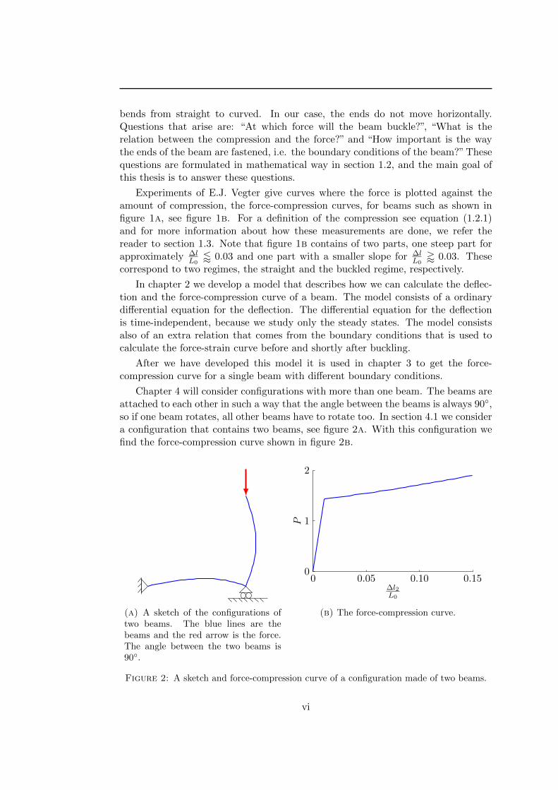
Chapter 4 will consider configurations with more than one beam. The beams areattached to each other in such a way that the angle between the beams is always 90◦,so if one beam rotates, all other beams have to rotate too. In section 4.1 we considera configuration that contains two beams, see figure 2a. With this configuration wefind the force-compression curve shown in figure 2b.

(a) A sketch of the configurations oftwo beams. The blue lines are thebeams and the red arrow is the force.The angle between the two beams is90◦.

0 0.05 0.10 0.15∆l2L0

P

0

1

2

(b) The force-compression curve.

Figure 2: A sketch and force-compression curve of a configuration made of two beams.

vi

CHAPTER 0. PREFACE

In section 4.2 we consider rubber networks with holes, as in figure 3a. But a piece

(a) A network of rubber of around11.5 by 10 centimetres.

0 5 10 15 200

10

20

30

∆l (mm)

P (N)

(b) A force-compression curve of a rubber net-work. For a detailed explanation see figure 4.5.

Figure 3: A photo of a rubber network and the corresponding force-compression curve.

of rubber with holes is not obviously a configuration of many beams. However, if wedo not look at the holes but at the rubber between the holes we can approximatethese thin pieces by beams. The larger blocks are the connections between thebeams. The experimental data of the force-compression curve is shown in figure 3b.For an explanation of the two different curves and the arrows, we refer the readerto section 4.2. In particular, we will compare the force-compression curve to that ofa single beam.

Chapter 5 and 6 contain the discussion and the conclusion.

vii

Chapter 1

Introduction

1.1 Compression of a piece of rubber

In this section, we will investigate a piece of rubber with length L0, and with con-stant cross-section over the entire length with a cross-section area A0, as shown infigure 1.1a. When a normal force N is applied at the ends, perpendicular to thecross-section, the piece of rubber shrinks. Let L be the new length after applyinga force and ∆L = L0 − L the deformation of the length between the uncompressedand the compressed piece, see figure 1.1b.

∆L

A0

L0

(a) A piece of rubber with length L0

and cross-section A0, over the entirelength.

A0

L

∆L

N

(b) The compressed piece, N is thenormal force perpendicular to thecross-section. L is the compressedlength and ∆L is the deformation.

Figure 1.1: A piece of rubber. After applying a normal force N , the piece is compressed.

The rest of section 1.1 describes this relation between the normal force and thedeformation, and parametrize the spatial scales of the piece rubber.

1.1.1 Hooke’s law

The physicist Hooke (1635-1703) described that for a spring the force is linear tothe compression. This relation is known as Hooke’s law. This theory is described inmore detail in the book [TG70]. This first order linear approximation of the relationbetween the compression and the force is very accurate for a spring, and also for a

1

1.1. COMPRESSION OF A PIECE OF RUBBER

lot of other materials. Every material where this first order linear approximationof the response to an applied force is accurate are called linear-elastic or Hookean.This approximation works only for forces that are not too large, because a materialcan not be stretched infinitely long, or compress to zero length. Rubber appears tobe a Hookean material, so the relation between N and ∆L is linear:

N ∝ ∆L. (1.1.1)

Two equal pieces placed behind each other become both ∆L shorter when the sameforce as above is applied, the total deformation is two times larger. In general wesee that the normal force is linear in the strain, ∆L

L0:

N ∝∆L

L0. (1.1.2)

The proportionality constant is now independent of the length of the piece. However,two pieces placed beside each other get both half of the force. In this case both piecesdeform half as much as first. Or more general using the stress N

A0, instead of the

force gives a proportionality constant independent of the area:

N

A0∝

∆L

L0. (1.1.3)

Here the proportionality constant is independent of all the spatial scales of the pieceof rubber. We define the hardness of any material, the Young’s modulus, E, as thestress per strain.

E ≡ N

A0

/∆L

L0. (1.1.4)

Using the Young’s modulus we get:

N

A0= E

∆L

L0. (1.1.5)

This relation between the stress and the strain is known as the generalized Hooke’slaw.

In this thesis the force is used instead of the stress, so we rewrite (1.1.5) to:

N = EA0∆L

L0. (1.1.6)

Equation (1.1.6) is an important result that tells us how some pieces of rubberresponded to a force. The condition that the force is not large is not a problembecause in this thesis the forces will be small.

Rather than considering the whole piece of rubber we can look to an infinitesimalpiece. Looking to the rate of change of the length at a single point, defined as thelocal strain, ε, and to stress, σ, at a point. The compression and the force can be

2

CHAPTER 1. INTRODUCTION

expressed by the local strain and the stress by integrating over the length or thecross-section of the beam:

∆L =

∫ L

0εdx, (1.1.7)

N =

∫∫A0

σdA0. (1.1.8)

For such an infinitesimal piece equation (1.1.5) becomes

σ = Eε, (1.1.9)

and relation (1.1.9) is the local Hooke’s law.

1.2 Buckling of a beam

In the previous section the response of a thick piece of rubber to a force is described.It becomes much more interesting when we look to a thin piece. In this thesis arectangular cuboid piece is used. The height, h, is small in comparison with thelength, L0, and the width, b. This piece is called a beam, see figure 1.2a.

L0h

b

xz

y

(a) A rubber beam with length L0,height h and width b, where h is rel-ative small in comparison with L0

and b.

Begin point

End point

Ll

h

b

xz

y

P

(b) The compressed, buckled beam, Pis the force parallel to the x-axis. Lis the compressed length and l the dis-tance between the ends of the beam.

Figure 1.2: Sketch of a beam. After applying a force P , the piece is compressed andbuckled.

For a force P parallel to the x-axis we expect that by increasing the force, thebeam is not only compressing, but that the beam will buckle at some moment.

As in the previous section, L is the length of the beam. This is the real lengthtaking into account the curvature. The distance between the two ends of the beamwe call l. See the sketch in figure 1.2b. Note that if the beam is not buckled, L andl are equal, and after buckling it holds that L > l.

The buckling of the beam is an interesting phenomenon. Engineers want to knowat which force a steel beam will buckle. This property indicates how strong a steelbuilding is, for when a supporting beam buckles the building collapses.

A second thing is the changing of the response of force in a beam. Because ofthe difference on a straight and a buckled beam, maybe (rubber) beams can be usedto make car bumpers, which are normally hard, but soft on impact.

3

1.2. BUCKLING OF A BEAM

1.2.1 Buckling load

We are interested in the question at what force the beam buckles. We will call thisforce the buckling load, Pc. How to define this force? If you press very careful it ispossible to compress the beam more and more without buckling of the beam. Thisis similar to balancing a ball on the top of a hill. Most of the time the ball will rolldown, because the potential energy decreases if the ball rolls to the foot of the hill.For a force that is larger than the buckling load, a straight beam has a potentialenergy that is larger than for a buckled beam, so the beam buckles. Figure 1.3gives a sketch of the potential energy for a force that is smaller than the bucklingload, 1.3a, and for a force that is larger than the buckling load, 1.3b.

Epo

Deflection

(a) The energy landscape for aforce smaller than the bucklingload. The only steady state is abeam without deflection and this isstable one.

Epo

Deflection

(b) The energy landscape for aforce larger than the buckling load.There are three steady states. Theunstable one is the straight beam,and for the stable state the beam isbuckled.

Figure 1.3: The energy landscape before and after buckling. The dots are the steadystates, the stable states in green and the unstable in red.

For a beam it holds that if the force is lower than the buckling load there is onlyone possible situation, the straight one. If the force is larger than the buckling loadthere are three possible situations, a straight and two buckled situations. The beamcan buckle to the positive and to negative z-direction. Because of symmetry thereare no differences in the potential energy between this two buckled situations.

This observation about the bifurcation allows us to define the buckling load asthe force at the bifurcation point. At a lower force there is one steady situation,by a larger force there are three steady situations. The beam buckles because thepotential energy of the buckled situations is lower than that of the straight one.

1.2.2 Engineering strain

In section 1.1 we have seen that the strain is a useful quantity. But for a buckledbeam we want to look to the distance between the ends of the beam instead of thelength of the beam. In analogy with the strain we will define the ‘engineering strain’as the decrease of the distance between the two ends divided by the length of the

4

CHAPTER 1. INTRODUCTION

uncompressed beam:

Engineering strain =∆l

L0=L0 − lL0

. (1.2.1)

We have already seen in the preface that the graph of the force versus the com-pression, or after scaling the engineering strain, contains two parts. One of thereasons why the slope after buckling is much smaller than before buckling is becauseafter buckling the engineering strain increase more than the strain. We will abbre-viate the force-engineering strain curve to ‘f-s curve’, note that the ‘s’ mains theengineering strain and not the strain.

Note that we can express l in ∆lL0

by inverting relation (1.2.1):

l = L0 − L0∆l

L0= L0

(1− ∆l

L0

). (1.2.2)

1.2.3 Schematic representation

The rest of the thesis we will represent the beam schematically. For this, it isnecessary to know in which directions the beam buckles. The beam will buckle inthe direction where the minimum force is required.

The second moment of area tells how hard it is to bend the beam. This secondmoment of area depends on the direction in which the beam is buckled. In section 2.2we will show that for buckling in the z-direction the second moment of area is thesmallest. This because the width is larger than the height. So the beam will bucklein the z-direction.

We can create a schematic representation of the beam. The beam buckles inthe z-direction so the y-coordinate is not interesting for investigation, and so wecan restrict ourselves to the xz-plane. Secondly we will look at the z-coordinate ofthe middle between the bottom and top of the beam for all x-values. We can nowmodel the beam as an one dimensional line in the xz-plane, see figure 1.4. We will

Begin point

End pointl

xz

y

(a) A three dimensional beam, theblue line is the middle of the beam.

w

z

x0 l

(b) A schematic representation ofthe beam. The blue line is the mid-dle of the beam. w(x) is the deflec-tion of the beam at the point x.

Figure 1.4: From a three dimensional beam to the schematic representation in the xz-plane, where for all x-values we have w(x) as the z-value of the middle of the beam.

describe the z-coordinate of the beam as function of x, where x ∈ [0, l]. We call thisz-coordinate the deflection of the beam, w(x). Note that if the beam is not buckledwe have w(x) = 0 for all x.

5

1.3. EXPERIMENTS

1.3 Experiments

The experimental data used in this thesis, are produced by other researchers ofthe research group “Complex Media”. The experiments are done using an accuratecompression machine from the Instron 5965-series, shown in figure 1.5. It can slowly

Figure 1.5: The Instron 5960-series. The sample is compressed by the Instron controller.The Instron is used to measure the f-s curves.

compress the beam and measure the force. Because the compression is slow thebeam is always in equilibrium (quasi-steady state), so there is no time dependence.

Photos of a beam and a network that we use are shown in figure 1.6.

(a) A front view of asingle beam.

(b) A photo of a network what we use. The beamsare the parts of rubber between the holes.

Figure 1.6: Two pictures of rubber configurations.

6

Chapter 2

Theory of the buckling of a beam

In this chapter we will deduce a model that describes the deflection and the f-scurve of a beam. The model uses the bending moment of the beam, the force andmoment balance of a beam in equilibrium and the fact that the stable situation isthat situation where the potential energy is minimal.

A important approximation that we make is that the deflection and its derivativeare small. This limits the use of the model in such a way that we can only use itbefore and short after buckling. A second condition will be that the beam is thin.

2.1 Moment of the beam

A bended beam has a tendency to bend back to a straight beam. The quantity thattells how strong this tendency is, is called the bending moment of the beam, or themoment.

First we will describe how we can calculate the moment in general and why abended beam has moment, and after that we will calculate the moment of a beamas function of the deflection using the curvature of the deflection w.

2.1.1 Bending moment

Suppose we have a lever with a rotation point R and an arm r. Applying a forceP at the endpoint of the arm Q, perpendicular to this arm, gives the tendency torotate, see figure 2.1a. The moment M is equal to the product of the force and thearm:

M = Pr. (2.1.1)

In a more general case the force is distributed over an area. In this case therotation is around a rotation axis, called R. This is shown in figure 2.1b. σ is thestress, the force density, and r the distance between an infinitesimal area dA andthe line. We can calculate the moment by integrating the stress times the distanceover the whole area:

M =

∫∫AσrdA. (2.1.2)

7

2.1. MOMENT OF THE BEAM

r

R

P

Q

M

(a) A lever with a rotation point R andan arm r. There is a force P at theendpoint Q, perpendicular to this armr. In this case we have M = Pr.

A

R

M

dA

r

σ

(b) An area A that rotate around theline R. The stress σ is orthogonal tothe area A. For the moment we have:M =

∫∫AσrdA.

Figure 2.1: The moment for a point and for an area by applying a force.

In our case the beam is in equilibrium, so the moment that comes from theapplied force have to be compensated by the beam itself. We therefore find for themoment of the beam:

Mbeam = −∫∫

AσrdA. (2.1.3)

To see why a bended beam has a moment we will take a look at figure 2.2. Thebeam has a height h, so if it is bent the inside is shorter than the outside, s1 < s2.A consequence of this is that the inside is under more compression than the outside.

L

s2

s1

hInside

Outside

σ

M

z

x

Figure 2.2: A front view of a bended beam. Since that the inside bend is shorter than theoutside bend we have s1 < L < s2. This causes that the stress on the inside is larger thanon the outside. If the beam is in equilibrium there is a moment of the beam to compensatethis.

From the local Hooke’s low (1.1.9) it follows that the stress at the inside is largerthan at the outside. So the stress is not distributed equally over the cross-section,and this difference gives a moment, which the beam has to compensate.

2.1.2 Calculating the moment

The hard part of this subsection is to calculate the difference in the strain betweenthe in- and outside bend. Ones we know this,we can use Hooke’s law, (1.1.9), to getthe stress.

8

CHAPTER 2. THEORY OF THE BUCKLING OF A BEAM

For an arc the length is known if the radius ρ and the angle in radians θ of thearc:

s = ρθ. (2.1.4)

Let us assume that the beam is curved as an arc, as shown in figure 2.3, with ρ theradius at the middle of the beam and r the distance from a point to the middle ofthe beam.

s(r)r

θ

ρ

Figure 2.3: A circular beam. ρ is the radius and s(r) is the arc length, r from the middleof the beam.

If we call the strain which is caused by the bending εb(r) we get:

εb(r) =s(0)− s(r)

s(0)=ρθ − (ρ+ r)θ

ρθ= −r

ρ. (2.1.5)

There is only one problem, a whole buckled beam does not have the shape of anarc. If we look at a short piece of the beam, we can approximate the shape of thatpart of the beam with a circle, just like that we can approximate it with the theoremof Taylor. This is done for point X in figure 2.4. For the point Y it will appearsthat a straight line is the best approximation, i.e. a circle with infinite radius.

The radius of the circle that fits the curve the best is called the radius of curva-ture. Instead of the radius of curvature we will use the reciprocal of it, the curvaturek = 1

ρ . k can be interpreted as the sharpness of the bend in the curve. For a straightline the curvature is zero.

We can calculate k using (2.1.4). If we take the limit where the arc length s goesto zero and look to how much the angle changes with respect to a change of the arclength we get:

k ≡ dθ

ds=

1

ρ. (2.1.6)

9

2.1. MOMENT OF THE BEAM

ρ

Xk = 1

ρ

Yk = 0

Figure 2.4: The curvature of a curve at two points. For one point there fits a circle withradius ρ, and for the other point a straight line.

Now we will calculate k at a point with x-coordinate x as a function of w(x):

k(x) =dθ

ds

∣∣∣∣x=x

=dθ

dx

∣∣∣∣x=x

dx

ds

∣∣∣∣x=x

=dθ

dx

∣∣∣∣x=x

(ds

dx

∣∣∣∣x=x

)−1

. (2.1.7)

The angle can be calculated using the tangent:

θ = arctan

(dy

dx

)= arctan(wx), (2.1.8)

Where we have used the subscript notation of the derivative: dwdx = wx. So this

gives:

dθ

dx=d arctan(wx)

dx=

1

1 + w2x

wxx. (2.1.9)

For dsdx we can use the theorem of Pythagoras:

ds2 = dx2 + dy2. (2.1.10)

And this implies: (ds

dx

)2

= 1 + w2x. (2.1.11)

And so

ds

dx=√

1 + w2x (2.1.12)

Substituting (2.1.9) and (2.1.12) in (2.1.7) gives:

k(x) =1

1 + wx(x)2wxx(x)

1√1 + wx(x)2

(2.1.13)

=wxx(x)

(1 + wx(x)2)3/2(2.1.14)

10


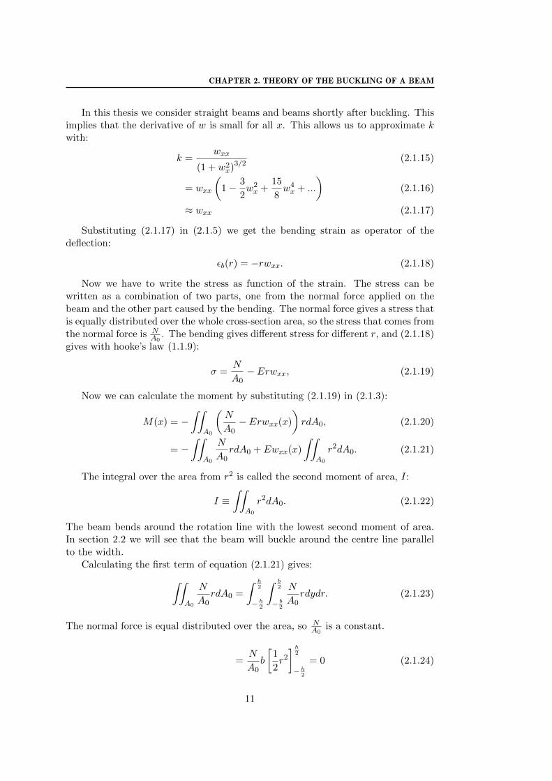
In this thesis we consider straight beams and beams shortly after buckling. Thisimplies that the derivative of w is small for all x. This allows us to approximate kwith:

k =wxx

(1 + w2x)3/2

(2.1.15)

= wxx

(1− 3

2w2x +

15

8w4x + ...

)(2.1.16)

≈ wxx (2.1.17)

Substituting (2.1.17) in (2.1.5) we get the bending strain as operator of thedeflection:

εb(r) = −rwxx. (2.1.18)

Now we have to write the stress as function of the strain. The stress can bewritten as a combination of two parts, one from the normal force applied on thebeam and the other part caused by the bending. The normal force gives a stress thatis equally distributed over the whole cross-section area, so the stress that comes fromthe normal force is N

A0. The bending gives different stress for different r, and (2.1.18)

gives with hooke’s law (1.1.9):

σ =N

A0− Erwxx, (2.1.19)

Now we can calculate the moment by substituting (2.1.19) in (2.1.3):

M(x) = −∫∫

A0

(N

A0− Erwxx(x)

)rdA0, (2.1.20)

= −∫∫

A0

N

A0rdA0 + Ewxx(x)

∫∫A0

r2dA0. (2.1.21)

The integral over the area from r2 is called the second moment of area, I:

I ≡∫∫

A0

r2dA0. (2.1.22)

The beam bends around the rotation line with the lowest second moment of area.In section 2.2 we will see that the beam will buckle around the centre line parallelto the width.

Calculating the first term of equation (2.1.21) gives:∫∫A0

N

A0rdA0 =

∫ h2

−h2

∫ b2

− b2

N

A0rdydr. (2.1.23)

The normal force is equal distributed over the area, so NA0

is a constant.

=N

A0b

[1

2r2

]h2

−h2

= 0 (2.1.24)

11

2.2. SECOND MOMENT OF AREA

Substituting the definition of I, (2.1.22), gives:

M(x) = EIwxx(x), (2.1.25)

We will use equation (2.1.25) to get the differential equation in the model of Euler-Bernoulli in section 2.3 and for the boundary conditions to solve the differentialequation.

2.2 Second moment of area

The second moment of area depends on the rotation line. This section tells us forwhich rotation line the second moment of area is minimal.

The beam will bend in the way that the second moment of area is as small aspossible. The second moment is the integral of r2, and for r2 it holds that:

1. it is always non-negative,

2. decreasing for r smaller than zero,

3. increasing for r larger than zero.

And so for a minimal second moment of area the rotation line is the line where allthe point of the area are as close as possible by that line. For a rectangle piece thisgives that the rotation line is the in the middle of two parallel sides of the rectangle,for R parallel to the width it gives figure 2.5:

h

12h

b

R

Figure 2.5: A rectangle with height h and width b. The rotation line R is in the middleat height 1

2h.

The second moment of area corresponding to the case of figure 2.5 is called Ihbecause the bending is in the h direction. Ib corresponds to the case where the areais turned a quarter.

Calculating Ih gives:

Ih =

∫∫A0

r2dA0 =

∫ h2

−h2

∫ b2

− b2

r2dydz = b

[1

3r3

]h2

−h2

=1

12bh3. (2.2.1)

Ib works at the same way and gives:

Ib =1

12hb3. (2.2.2)

12


And so we get:

IhIb

=h2

b2=

(h

b

)2

. (2.2.3)

For the beam we assume that h is smaller than b, so we get:

Ih < Ib. (2.2.4)

Altogether we know that Ih is the smallest second moment of area, so the beamwill bend around the h direction. And so the bending is in the xz-plane.

2.3 Euler–Bernoulli, force and moment balance

Euler and Bernoulli have developed a theory for buckled beams using the balance ofthe force and the moment. The beam is in equilibrium so the net force and momenthave to be zero. For the moment balance we use the result of section 2.1. This givesa differential equation for the deflection w, as we will show in subsection 2.3.1.

2.3.1 Force and moment balance

This subsection is closely analogous to the first chapter of the book [BC10], wherethe derivation of the differential equation is calculated in a more general setting.

Let’s take a beam like the one in figure 2.6. Let P0, V0 and M0 are the horizontalforce, the vertical force and the moment at the endpoint of the beam respectively.P (x), V (x) and M(x) are the forces and moment as a function of x.

wP0

PV

V0

M0

Mx

Figure 2.6: A beam where at x = 0 we apply the horizontal and vertical forces P0 and V0

and a moment M0. For every x value there are P , V , and M . These forces and momentshave to be balanced.

The beam is in equilibrium, so the net force and moment are zero. The balanceof the forces is quite easy:

P (x) = P0, (2.3.1)

V (x) = V0. (2.3.2)

So this implies that the horizontal and the vertical force are constant:

Px(x) = 0, (2.3.3)

Vx(x) = 0. (2.3.4)

13

2.3. EULER–BERNOULLI, FORCE AND MOMENT BALANCE

For the balance of the moment we have to take both the moment and the forcesinto account. The forces play a role because the forces have an arm to the rotationpoint, so they give a moment too. Let’s look at a rotation around the begin point ofthe beam by x = 0. The forces P0 and V0 have no arm with respect to the rotationpoint so they do not give a moment. For the vertical force V (x) for general x thelength of the arm is x, and for P (x) the length of the arm is w(x). So together withthe moment M0 and M(x) it gives:

M(x) + P (x)w(x) + V (x)x−M0 = 0. (2.3.5)

P (x) is a constant, so we will write P instead. There are two unknown constantsin this equation, M0 and V (x) = V0. We will differentiate equation (2.3.5) twiceto remove the constants. This increases the order of our differential equation. Theadvance is that we now can use other boundary conditions than V0 and M0 too.Differentiating twice gives:

Mxx(x) + Pwxx(x) = 0. (2.3.6)

Now we can substitute the equation for the moment, (2.1.25), found in section 2.1,to get:

[EIwxx(x)]xx + P (x)wxx(x) = 0. (2.3.7)

E and I are constants, so we get:

EIwxxxx(x) + Pwxx(x) = 0. (2.3.8)

This is the fourth order differential equation that describes the deflection of thebeam. To reduce the writing we introduce the constant k, defined through k2 ≡ P

EI :

wxxxx + k2wxx = 0, (2.3.9)

k2 ≡ P

EI. (2.3.10)

2.3.2 General solution of the differential equation

A brief look to (2.3.9) tells us that the fourth order differential equation reduces toa second order equation if we introduce v as the second derivative of w:

v ≡ wxx. (2.3.11)

Substituting v in equation (2.3.9) gives a very well known second order differentialequation:

vxx + k2v = 0. (2.3.12)

If k is not zero, or equivalently if P > 0, the solution is:

v(x) = A sin(kx) + B cos(kx). (2.3.13)

14


Now we can integrate (2.3.13) twice to get w, this adds a linear and a constant term:

w(x) = A sin(kx) +B cos(kx) + Cx+D, if P 6= 0. (2.3.14)

Sometimes there is no pressing force P . In that case the solution of (2.3.9) is a thirddegree polynomial:

w(x) = ax3 + bx2 + cx+ d, if P = 0. (2.3.15)

In (2.3.14) we see that k is not only a constant which reduces writing, but thatk can be interpreted as the wave number, so a larger force gives more waves in thedeflection of the beam.

2.4 The force-strain curve

Now that we know the differential equation that describes the deflection of the beamfor a given force it is time to calculate the f-s curve. We will see that a non-zerodeflection is only possible if the force and the engineering strain are related to eachother in a special way. This relation is the key to the f-s curve.

2.4.1 Straight regime

For a straight beam the deflection is zero, w = 0. The straight beam satisfies thedifferential equation (2.3.8) for all P because both sides will equal zero, and generallyw = 0 satisfies the boundary conditions too.

In the straight regime the slope can be calculated by using (1.1.6). This formulaappliers because the beam is straight, L = l, and so ∆L

L0= ∆l

L0, and because the fact

that the normal force is parallel to the x-axis. The second observation gives thatthe normal force N is equal to the force P . Substituting this two things in (1.1.6)gives:

P straight = EA0∆l

L0. (2.4.1)

So for the straight regime the f-s curve is a line through the origin.

2.4.2 Buckled regime

For a buckled beam, we can solve differential equation (2.3.9), by using the generalsolution for non-zero force, (2.3.14). We have to calculate the four constants for somegiven boundary conditions. There are four constants, so we need four boundaryconditions. For example a beam whose ends are mounted on hinges and the hingeson the x-axis. This gives a beam where the deflection and the moment are zero atthe ends: w(0) = w(l) = M(0) = M(l) = 0. This is elaborated in section 3.1. Thisboundary conditions with (2.3.14) gives a system of four equations.

If we now solve this system the trivial solution where the beam is a straight line,w = 0, is always allowed and for some specific wave numbers there is also a non-zero

15

2.4. THE FORCE-STRAIN CURVE

solution. By these k’s the last boundary conditions is always satisfied and there isno unique solution.

For a buckled beam, k has to be one of these specific numbers. The specificvalues of k depend on l, so this gives a relation between k and l. If we change l,k has to be changes in such a way that the relation is still true. Rewriting thisequation between k and l using the definitions of k (2.3.10), and the engineeringstrain (1.2.1) gives a relation between the force and the engineering strain. This willgive the f-s curve for a buckled beam.

2.4.3 Boundary between the two regimes

Now we have two f-s curves, one for the straight regime and one for the buckledregime. For a hinged beam in section 3.1 the curves are shown in figure 2.7, the greenand the blue lines correspond to the straight and the buckled regime respectively.

0 0.05 0.1 0.15∆lL0

P

((

∆lL0

)

c, Pc

)

Pe

Figure 2.7: The f-s curve of a hinged beam. Here the green line corresponds to the straightregime and the blue line corresponds to the buckled regime. The red point is the momentwhere the beam buckles.

In physical systems with multiple possible configurations the most stable situa-tion is that situation with the lowest potential energy. The potential energy can bycalculated by integrating the force over the distance over which the endpoint of thebeam has moved:

Epo =

∫ ∆l

0Pdx. (2.4.2)

So the lowest potential energy implies that the force was minimal during the wholecompression. For small engineering strain the force from the straight regime is the

16


lowest, and for large engineering strain the force for the buckled regime. The pointwhere the two forces are equal is the point where the beam becomes buckled, thered point in figure 2.7. The corresponding force is the buckling load Pc.

And for the general f-s curve we get:

P = min{P straight, P buckled

}. (2.4.3)

The slope of P straight is much larger than the slope of P buckled. This implies thatP buckled(0) is a good approximation of the buckling load.

17

2.4. THE FORCE-STRAIN CURVE

18

Chapter 3

Configurations with a single beam

In this chapter we will start to address the main goal of this thesis. The model that isdeduced in chapter 2 can be used to calculate the f-s curves for several configurations.The difference between the situations is the way in which the ends of the beam arefastened to the press, represented by different boundary conditions.

In the first section we will treat a beam fastened with two hinges, such that theends of the beam can rotate freely. In the second section a rotational spring is addedat one end. We will see that this increases the buckling load.

3.1 Hinged beam

A schematic overview of a hinged beam is given in figure 3.1. The hinges are depictedas triangles.

x-axis0 l

P

Figure 3.1: Sketch of hinged beam. The deflection on the ends is zero, but both ends canrotate freely.

3.1.1 Solving the differential equation

To solve the differential equation for chapter 2, given in (2.3.9), it is needed to writethe boundary conditions in terms of w. For a hinged beam, figure 3.1, the hingesare placed on the x-axis and fastened on the ends of the beam, so the deflections atthe ends are zero:

w(0) = w(l) = 0. (3.1.1)

19

3.1. HINGED BEAM

A hinge can rotate, so the moment on the endpoints is zero. From equation (2.1.25)it follows that

EIwxx(0) = EIwxx(l) = 0. (3.1.2)

So:

wxx(0) = wxx(l) = 0. (3.1.3)

Now the boundary conditions are known, it is possible to solve (2.3.14) with theboundary conditions (3.1.1) and (3.1.3). For x = 0:

w = A sin(kx) +B cos(kx) + Cx+Dw(0) = wxx(0) = 0

}⇒ w = A sin(kx) + Cx. (3.1.4)

And at x = l we get:

w = A sin(kx) + Cxw(l) = 0

}⇒ w = A

(sin(kx)− sin(kl)

lx

). (3.1.5)

The last boundary condition gives:

0 =

[A

(sin(kx)− sin(kl)

lx

)]xx

∣∣∣∣x=l

= −k2A sin(kl). (3.1.6)

Since we apply a force k is not zero and equation (3.1.6) implies

A = 0 or sin(kl) = 0. (3.1.7)

If A = 0 the deflections reduces to w(x) = 0. But then the beam is not buckled. Withother words, for a buckled beam is A non-zero. From that we get that sin(kl) = 0,so kl = nπ with n ∈ Z. If n = 0 we get w = A sin(0) = 0, so for the same reason aswhy A differs from zero, n differs from zero.

The minus sign of n can be absorbed in A, so without lose of generalization wecan take n ∈ N = {1, 2, ...}. In conclusion, the deflection is:

w(x) = A sin (kx) , (3.1.8)

k =nπ

lwith n ∈ N. (3.1.9)

Note that the A in formula (3.1.8) is undetermined. In some similar problemscalculating a higher order of w using perturbation theorem gives more informationabout an undetermined constant. In this thesis this is not done.

3.1.2 Force-engineering strain curve

For the straight regime there is found that the f-s curve is given by (2.4.1). Forthe buckled regime the f-s curve can be calculated with the relation between k and

20

CHAPTER 3. CONFIGURATIONS WITH A SINGLE BEAM

l given in equation (3.1.9) to derive the f-s curve. We use equations (2.3.10) and(1.2.2) to eliminate k and l to get:

P buckled = EI

nπ

L0

(1− ∆l

L0

)2

= EI

(π

L0

)2(

n

1− ∆lL0

)2

. (3.1.10)

Equation (3.1.10) gives the force as a function of the engineering strain, but thereis a dependence on the number n. The number n indicates the mode of the beam,if n is equal to one the beam is in the first mode, n = 2 gives the second mode, andso on. The first three modes are plotted in figure 3.2.

0 l

Figure 3.2: The first three modes of a beam, the blue line is the first mode where n = 1,the red line the second mode and the green line is the third mode.

Now the question is: ‘With mode is seen in in an experiment?’ In section 2.4there is noted that the most stable configuration is those with the lowest potentialenergy and this implies that the beam is in the configuration corresponding to thelowest force. For the case of the modes of the beam this implies that the beam prefersto be in the lowest mode. Taking n equal to one gives the formula in (3.1.11).

P buckled = EI

(π

L0

)2 1(1− ∆l

L0

)2 . (3.1.11)

This formula is sketched as the blue line in figure 3.3, the green line is the f-s curvefor a straight beam and the red point the buckling point.

Substituting the force for a straight beam (2.4.1), and that for a buckled beam (3.1.11)in equation (2.4.3) gives the f-s curve before and after buckling:

P = min

EA0∆l

L0, EI

(π

L0

)2 1(1− ∆l

L0

)2

. (3.1.12)

3.1.3 Relative force

It is useful to scale the force such that all beams buckle around the same value, evenif the beams have different dimensions or are made of rubber with different Young’smodulus. An approximation of the buckling load is used to scale the force.

The slope before buckling is much larger than after buckling, so the force for abuckled beam with engineering strain zero is a good approximation for the bucklingload:

Pc ≈ P buckled(0). (3.1.13)

21

3.1. HINGED BEAM

0 0.05 0.1 0.15∆lL0

P

((

∆lL0

)

c, Pc

)

Pe

Figure 3.3: The f-s curve of a hinged beam, where the green line is the straight regime,and the blue one the buckled regime. The red point is the buckling point and Pe is the Eulerload of this beam.

This approximation is called Euler load,

Pe ≡ P buckled(0) = EI

(π

L0

)2

. (3.1.14)

We now define the relative force as the force divided by the Euler load:

Pr ≡P

Pe. (3.1.15)

Using the definition of the relative force we get for the straight regime:

P straightr =

EA0∆lL0

EI(πL0

)2 =A0

I

(L0

π

)2 ∆l

L0. (3.1.16)

For the buckled regime we find:

P buckledr =

EI(πL0

)21(

1−∆lL0

)2

EI(πL0

)2 =1(

1− ∆lL0

)2 . (3.1.17)

Note that after this scaling the relative force is independent of the Young’s modulusand in the buckled regime the force does not depend on the dimensions of the beam.

22


Short after buckling is the engineering strain small, so a Taylor approximationof P buckled

r gives the slope of the relative force-engineering strain curve (rf-s curve)after buckling:

P buckledr ≈ 1 + 2

∆l

L0. (3.1.18)

So the slope of the rf-s curve is 2 after buckling.

Sometimes it is useful to write k as function of the relative force. We see that:

k2 =P

EI=PrPeEI

=PrEI

(πL0

)2

EI= Pr

(π

L0

)2

, (3.1.19)

or

k =π

L0

√Pr. (3.1.20)

3.2 Hinged beam with rotational spring

In this section a rotational spring is added to the configuration of section 3.1. Arotational spring gives a moment against the rotation that is proportional to therotational angle. See the sketch in figure 3.4. The spring is represented by the spiraland θ is the angle of the beam with the x-axis at x = l. The spring is placed at thepoint x = l because this gives an easier formula for w(x) later, but x = 0 would givethe same f-s curve.

x-axis0 l

Pθ

Figure 3.4: Sketch of hinged beam with a rotational spring to one endpoint of the beam.The deflections on the ends are zero. The spring applies a momentum which causes that thebeam buckles at a larger force.

3.2.1 Boundary conditions

At both endpoints the deflection is zero because of the hinges,

w(0) = w(l) = 0. (3.2.1)

At x = 0 we know that the moment of the beam is zero because of the hinge,M(0) = 0. Equation (2.1.25) gives:

wxx(0) = 0. (3.2.2)

23

3.2. HINGED BEAM WITH ROTATIONAL SPRING

The spring applies a moment at the point x = l. The moment is proportional to theangle θ with the spring constant µ:

Mspring = −µθ. (3.2.3)

It holds that θ = arctan(−wx(l)). The deformations are small, so the linear approx-imation of the tangent is accurate.

Mspring ≈ −µ · −wx(l) = µwx(l). (3.2.4)

The moment of the beam has to balance this moment of the spring, so:

Mbeam = −µwx(l). (3.2.5)

Substituting the moment of the beam, (2.1.25), gives:

EIwxx(l) = −µwx(l), (3.2.6)

or

wxx(l) = − µ

EIwx(l). (3.2.7)

Defining the dimensionless quantity µ ≡ µL0

EI gives

wxx(l) = − µ

L0wx(l). (3.2.8)

This µ can be interpreted as the strength of the spring compared to the strength ofthe beam. In the rest of this section µ is called the spring constant instead of µ.

And (3.2.8) is the fourth boundary condition.

3.2.2 Solving the differential equation

We have to solve the differential equation wxxxx + k2wxx = 0 for this boundaryconditions. There is a force P so we can use the general solution given in equa-tion (2.3.14). Three of the four boundary conditions are the same as in section 3.1,this gives with (3.1.5):

w = A

(sin(kx)− sin(kl)

lx

). (3.2.9)

The last boundary condition, (3.2.8), gives:[A

(sin(kx)− sin(kl)

lx

)]xx

∣∣∣∣x=l

= − µ

L0

[A

(sin(kx)− sin(kl)

lx

)]x

∣∣∣∣x=l

. (3.2.10)

24


After some calculations this reduces to:

A = 0 or tan(kl) =kl

1 + k2lL0µ

. (3.2.11)

And for a buckled beam it holds that A 6= 0 and k > 0, so the solution for thedeflection is:

w = A

(sin(kx)− sin(kl)

lx

). (3.2.12)

Where k and l such that the following relation holds:

tan(kl) =kl

1 + k2lL0µ

. (3.2.13)

3.2.3 Relative force-engineering strain curve

With a spring, the force is not only depending on the engineering strain, but alsoon µ. To exhibit the underlying µ-dependence for the force an upper index (µ) isadded: P (µ). If µ is equal to zero the spring has no effect and the situation is thatof the hinged beam in section 3.1. So P (0) = P hinged. This gives that P (0)(0) = Pe

and for the relative force, P(µ)r

(∆lL0

), we have P

(0)r (0) = 1.

Equation (3.2.13) is a relation between k and l. Which can not be solved ana-lytical. We will consider the limit cases where the spring constant becomes zero orinfinity and later we will solve it numerical. In the limit µ→ 0 the relation (3.2.13)must simplify to the relation for a hinged beam. For the limit µ→∞ the endpointof the beam can not rotate, and the endpoint of the beam has to be tangent to thex-axis.

The limit for µ to zero

Looking at the right hand side (r.h.s.) of (3.2.13) if µ goes to zero we see that:

limµ↓0

kl

1 + k2lL0µ

= 0, (3.2.14)

and we get

tan(kl) = 0. (3.2.15)

And because tan(α) = sin(α)cos(α) , this implies

sin(kl) = 0, (3.2.16)

and (3.2.16) is equal to (3.1.7), so relation (3.2.13) reduces to the case for a hingedbeam. And with equation (3.1.17):

P (0)r

(∆l

L0

)= P hinged

r

(∆l

L0

)=

1(1− ∆l

L0

)2 . (3.2.17)

25


The limit for µ to infinity

For the limit µ to infinity, the r.h.s. of equation (3.2.13) reduces to:

limµ→∞

kl

1 + k2lL0µ

= kl, (3.2.18)

and so

tan(kl) = kl. (3.2.19)

Calculating wx(l), using (3.2.19) gives:

wx(l) =

[A

(sin(kx)− sin(kl)

lx

)]x

∣∣∣∣x=l

, (3.2.20)

= A

(k cos(kl)− sin(kl)

l

), (3.2.21)

= Acos(kl)

l(kl − tan(kl)) , (3.2.22)

= 0. (3.2.23)

So in this case the derivative at x = l is zero so the endpoint of the beam will betangent to the x-axis.

A second thing is that for µ → ∞ relation (3.2.13) reduces to a relation of klrather than a relation of k and l. So solving tan(α) = α gives k = α

l . tan(α) = α hasinfinity many solutions, but as for the hinged beam in section 3.1 the first non-zerosolution is the one that is seen in the experiments, and is called C,numerically wefind that C = 4.4934..., and so

k =C

l. (3.2.24)

The equations (1.2.2) and (3.1.20) give for the rf-s curve:

P (∞)r

(∆l

L0

)=

(C

π

)2 1(1− ∆l

L0

)2 . (3.2.25)

This differs only by a factor(Cπ

)2from Pr for a hinged beam:

=

(C

π

)2

P hingedr

(∆l

L0

)(3.2.26)

= 2.0457... · P hingedr

(∆l

L0

). (3.2.27)

So the buckling load and the slope after buckling for a beam with an infinitely strongspring are around 2 times as large as the buckling load for a hinged beam.

26


General µ

For general µ a numerical approximation is needed. To get the rf-s curve, firstequation (3.2.13) is written in terms of the engineering strain and the relative forceby using (1.2.2) and (3.1.20):

tan

(π

√P

(µ)r

(1− ∆l

L0

))=

π

√P

(µ)r

(1− ∆l

L0

)1 + π2

µ P(µ)r

(1− ∆l

L0

) . (3.2.28)

In figure 3.5 relation (3.2.28) is plotted for ∆lL0

= 0.05 and µ = 20. The blue line isthe l.h.s. and the green line is the r.h.s. The red dots are the intersections of thistwo lines and so the solutions of relation (3.2.28).

0 2 4 6 8 10 12 14 16 18 20 22−3

−2

−1

0

1

2

3

4

Pr

tan

(

π√

Pr

(

1−∆l

L0

))

π√

Pr

(

1−∆l

L0

)

1+π2

µPr

(

1−∆l

L0

)

Solutions

Figure 3.5: Graph of the l.h.s. of (3.2.28) in blue, and the r.h.s. in green. The intersectionsare shown in red.

Taking the first non-zero solution for a fixed spring constant µ and several valuesof the engineering strain ∆l

L0gives the rf-s curves for that specific spring constant.

For four µ values this curve is plotted in figure 3.6.

Now the relation between P(µ)r and ∆l

L0, and so between k and l, is known, it

can be used to calculate the deflection of the beam as function of x given in equa-tion (3.2.12). The result is shone in figure 3.7. The limit cases are the blue and thepurple lines. The blue line for µ = 0 gives a perfect sine, and the purple line forµ =∞ with wx(l) = 0.

3.2.4 The buckling load and the slope of the force-engineering strain curveafter buckling

An approximation of the buckling load is the intersection of the rf-s curve is figure 3.6

with the Pr-axis, with other words P(µ)r (0). This approximation as function of mu

is plotted as the blue line in figure 3.8.

27


0 0.05 0.1 0.150

0.5

1

1.5

2

2.5

∆l

L0

Pr

µ = ∞

µ = 10

µ = 2

µ = 0

Figure 3.6: The rf-s curves for a hinged beam with rotational springs of different strength.The blue, green, red and purple lines are with a strength of respectively 0, 2, 10 and ∞.

0 10 20 30 40 50 60 700.5

1

1.5

2

2.5

3

3.5

4

µ

P(µ)r (0)

P(µ)r

′

(0)

Figure 3.8: The blue line is the relative buckling load as function of µ. The green line isthe slope of the rf-s curve after buckling. If the beam is hinged, i.e. µ is zero, the relativebuckling load is one and the slope is two. For positive µ the relative buckling load and theslope increase.

If µ is zero, the buckling load is equal to the Euler load, so P(0)r (0) = 1. For µ

larger than zero the relative buckling load increases.

For the slope of the rf-s curve after buckling the theorem of implicit differentiationis used. This is done for equation (3.2.28) in appendix A. A plot of the slope of the

rf-s curve at zero strain as function of µ, P(µ)r

′(0), is given by the green line in

figure 3.8. If µ = 0, the slope equals 2, agreeing which our result from section 3.1,

28


0 1 2 3 4 50

0.25

0.5

0.75

1

x

w

µ = ∞

µ = 10

µ = 2

µ = 0

Figure 3.7: w(x) for different spring constants. The blue, green, red and purple lines arewith a constant of respectively 0, 2, 10 and ∞. For µ = 0 it is a sine and for µ = ∞ theslope is zero at the end.

for larger µ the slope is steeper.The relative force is the force scaled with the Euler load, an approximation of

the buckling load for a hinged beam. Now the buckling load is a function of µ, another scaling is the scaling with the approximation of the buckling load of a hingedbeam with a spring with spring constant µ:

P (µ)r

(∆l

L0

)=P (µ)

(∆lL0

)P (µ)(0)

, (3.2.29)

instead of

P (µ)r

(∆l

L0

)=P (µ)

(∆lL0

)Pe

=P (µ)

(∆lL0

)P (0)(0)

. (3.2.30)

If the force is scaled in this way the f-s curve becomes figure 3.9. Because of the

fact that P(∞)r

(∆lL0

)is a multiple of P

(0)r

(∆lL0

), this two lines collapse. The lines for

µ ∈ (0,∞) are lower than the lines for µ equal to zero or infinity.It appears that this rescaling has the nice property that the slope after buckling

is around 2 for all µ. A graph of the slope after buckling with this rescaling is givenin figure 3.10. Here f(µ) is the rescaled slope after buckling as function of µ:

f(µ) ≡ P(µ)r

′(0)

P(µ)r (0)

. (3.2.31)

The limits of f(µ) for µ to zero or to infinity are 2. For the calculations we referthe reader to appendix A.1. For µ ∈ (0,∞), f(µ) is smaller than two.

29


0 0.05 0.1 0.150.9

1

1.1

1.2

1.3

1.4

∆l

L0

P(µ

)r

P(∞)r

P(10)r

P(2)r

P(0)r

Figure 3.9: The rescaled f-s curves of a hinged beam with a rotational spring. The curvesfor µ = 0 and for µ = ∞ coincide. The slopes for µ equal to 2 and 10 are lower than theslopes for µ equal to zero or infinity.

0 10 20 30 40 50 60 701.75

1.8

1.85

1.9

1.95

2

µ

f(µ)

limµ→∞

f (µ) = 2

Figure 3.10: The slope of the f-s curve versus µ short after buckling, if the force is scaledwith P (µ)(0). If µ = 0 or µ =∞ the slope is 2, and for µ ∈ (0,∞) it is smaller than 2.

30

Chapter 4

Configurations with more beams

In this chapter we will consider configurations with two or more beams. The beamsare attached to each other in such a way that the angle between the beams is 90◦,so if the end of a beam rotates the beams that are attached to that beam have torotate with it. In the experiments the angle between the beams is fixed becausethe beams are connected to small cubes of rubber. These cubes are hard to bendbecause they are thick and short. So the beams will bend instead of the cubes andthe angle remains 90◦.

In section 4.1 we will discuss a configuration that contains two beams and insection 4.2 we will investigate a network containing several beams.

4.1 Two beams configuration

The configuration has a horizontal and a vertical beam, respectively beam 1 andbeam 2, see figure 4.1. A force P is pressing on the top of beam 1. The begin pointof beam 1 has the freedom to move horizontally. We expect that the buckling loadis larger than that of a single hinged beam, because beam 1 works like the springdescribed in section 3.2.

The angle between the x1-axis and beam 1 at x1 = l1 will be denoted with θ.Since the angle between the two beams is 90◦ the angle between the x2-axis andbeam 2 at x2 = l2 is also θ.

Instead of decreasing l and then calculating the corresponding k, as we have donein chapter 3, we will calculate a pair k, l2 for a given value of the angle θ in thissection. This gives a point in the rf-s plane. We will do this for different values ofθ, and all these points together will give us an rf-s curve.

4.1.1 Formulas for the deflections of the beams for a given angle.

Beam 1

There is no force acting on beam 1, so with (2.3.15) we get:

w1(x1) = ax31 + bx2

1 + cx1 + d (4.1.1)

31

4.1. TWO BEAMS CONFIGURATION

Beam 1

w1 = 0

Beam 2

w2 = 0

θθ

x1-axis0 l1

x2-axis

l2

0

P

Figure 4.1: Sketch of the two beams. l1 and l2 are the distances between the two end ofrespectively beam 1 and beam 2. θ is angle between the beams and the axes at the endpointsof the beams. The begin point of beam 1 can move freely in the horizontal direction, sothere is no horizontal force on beam 1.

The boundary conditions at x1 = 0 are w1(0) = 0; w1x1x1(0) = 0, so:

w1(0) = 0w1x1x1

(0) = 0

}⇒ b = d = 0. (4.1.2)

This gives: w1(x1) = ax31 + cx1. The boundary conditions at x1 = l1 are w1(l1) = 0

and w1x1(l1) = − arctan(θ) ≈ −θ for small θ:

w1(l1) = 0⇒ al31 + cl1 = 0w1x1

(l1) = −θ ⇒ 3al21 + c = −θ

}⇒ a = − θ

2l21, c =

θ

2. (4.1.3)

Altogether we have:

w1(x1) = − θ

2l21x3

1 +θ

2x1 =

θ

2x1

(1−

(x1

l1

)2). (4.1.4)

Beam 2

There is a force acting on beam 2, so (2.3.14) gives:

w2(x2) = A sin(kx2) +B cos(kx2) + Cx2 +D. (4.1.5)

The four boundary conditions are:

w2(0) = w2(l) = w2x2x2(0) = 0, (4.1.6)

w2x2(l) = − arctan(θ) ≈ −θ. (4.1.7)

32

CHAPTER 4. CONFIGURATIONS WITH MORE BEAMS

The first three boundary conditions are the same as for the hinged beam in sec-tion 3.1, so we can use result (3.1.5):

w2(x2) = A

(sin(kx2)− sin(kl2)

l2x2

). (4.1.8)

The fourth boundary condition gives:

w2x2(l2) = −θ ⇒ A = − θ

k cos(kl2)− sin(kl2)l2

. (4.1.9)

If we combine (4.1.8) and (4.1.9) we get the result for the deflection of beam 2:

w2(x2) = A


l2x2

), (4.1.10)

with

A = − θ


. (4.1.11)

4.1.2 The length of the beams

We can get more information about the deflection of the beams if we know thelength of them, i.e. L1 and L2. To calculate the length of the beams we will deducea general formula for the length of a beam as function of its deflecting. After thatwe will substitute the deflections of beam 1 and 2 in this general formula to get thelength of the beams.

General beam length

Let w(x) be the deflection of a beam between zero and l. For the length L we have:

L =

∫ds =

∫ l

0

ds

dxdx. (4.1.12)

Using the expression of dsdx that we get in section 2.1, (2.1.12), gives:

L =

∫ l

0

√1 + w2

xdx. (4.1.13)

Using the first order Taylor approximation of the square root, assuming that wx issmall, gives:

L ≈∫ l

01 +

1

2w2xdx, (4.1.14)

= l +1

2

∫ l

0w2xdx. (4.1.15)

33


The length of beam 1

For beam 1 there is no force to compress the beam, so we have L1 = L0. Now usingformula (4.1.4), we get:

L0 = L1 = l1 +1

2

∫ l1

0

([− θ

2l21x3

1 +θ

2x1

]x1

)2

dx1. (4.1.16)

After expanding the brackets and computing the integral we find:

l1 =L0

1 + θ2

10

. (4.1.17)

The length of beam 2

Equation (4.1.15) together with equation (4.1.10) gives:

L2 = l2 +1

2

∫ l2

0

([A


l2x2

)]x2

)2

dx2. (4.1.18)

We compute this integral and find:

L2 = l2 +1

8

A2

l2

(−2 + 2k2l22 + 2 cos(2kl2) + kl2 sin(2kl2)

). (4.1.19)

Now we have a relation between L2 and l2, but we don’t know L2. However, we canapproximate L2 using the force P and L0. We know L2 if we know the normal force.Formula (1.1.6): N = EA0

∆LL0

gives

L2 = L0

(1− N

EA0

). (4.1.20)

For small deflections the normal force is by approximation equal to the force P .

L2 ≈ L0

(1− P

EA0

). (4.1.21)

If we now use (2.3.10), the definition of k, we get for L2

L2 = L0

(1− I

A0k2

). (4.1.22)

Now combing (4.1.19) and (4.1.22), we get a relation for l2:

L0

(1− I

A0k2

)= l2 +

1

8

A2

l2

(−2 + 2k2l22 + 2 cos(2kl2) + kl2 sin(2kl2)

). (4.1.23)

34


4.1.3 Momentum balance

The point (l1, l2) is hinged, so there is no net momentum,

M1(l1) +M2(l2) = 0. (4.1.24)

For the momentum we know from (2.1.25) that M(x) = EIwxx(x). This gives forM1 and M2:

M1(l1)

EI=

[− θ

2l21x3

1 +θ

2x1

]x1x1

∣∣∣∣∣x1=l1

= −3θ

l1(4.1.25)

M2(l2)

EI=

[A


l2x2

)]x2x2

∣∣∣∣∣x2=l2

(4.1.26)

= −Ak2 sin(kl2) (4.1.27)

Balancing of the moment gives:

A =−3θ

l1k2 sin(kl2)(4.1.28)

4.1.4 Force-engineering strain curve

Beam 2 can be compressed without affecting beam 1, so all formulas in the straightregime are equal to those for a single beam computed in section 2.4.1. From this wefind the green line shown in figure 4.2.

For the buckled regime we will find a pair of k and l2 for different values of θ.For this we need a system of two equations as there are two unknowns, k and l2.From equations (4.1.11) and (4.1.28) we get:

A = − θ


A = −3θl1k2 sin(kl2)

⇒ k cos(kl2)− sin(kl2)

(1

l2+l1k

2

3

)= 0. (4.1.29)

Rewriting equation (4.1.29) gives a relation similar as in (3.2.19):

tan(kl2) =l2k

1 + 13 l1l2k

2. (4.1.30)

And this gives some values for k for given values of l1 and l2. By substituting (4.1.17)into (4.1.30) we can remove the l1 dependence:

tan(kl2) = l2k

/1 +

1

3

L0

1 + θ10

l2k2 . (4.1.31)

And we can use the equations (4.1.11) and (4.1.23) to get another relation be-tween k, θ and l2,(

l2 − L0

(1− I

A0k2

))(8l2

(k cos(kl2)− sin(kl2)

l2

)2)

+

θ2(−2 + 2k2l22 + 2 cos(2kl2) + kl2 sin(2kl2)

)= 0. (4.1.32)

35


Combining (4.1.31) and (4.1.32) gives the following system:tan(kl2) =l2k

/1 + 1

3L0

1+ θ10

l2k2

0 =(l2 − L0

(1− I

A0k2))(

8l2

(k cos(kl2)− sin(kl2)

l2

)2)

+θ2(−2 + 2k2l22 + 2 cos(2kl2) + kl2 sin(2kl2)

) (4.1.33)

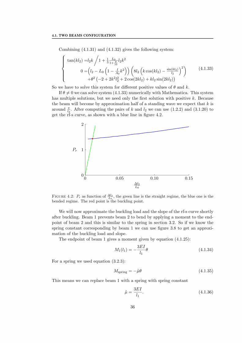
So we have to solve this system for different positive values of θ and k.If θ 6= 0 we can solve system (4.1.33) numerically with Mathematica. This system

has multiple solutions, but we need only the first solution with positive k. Becausethe beam will become by approximation half of a standing wave we expect that k isaround π

l2. After computing the pairs of k and l2 we can use (1.2.2) and (3.1.20) to

get the rf-s curve, as shown with a blue line in figure 4.2.

0 0.05 0.10 0.15∆l2L0

Pr

0

1

2

Figure 4.2: Pr as function of ∆l2L0

, the green line is the straight regime, the blue one is thebended regime. The red point is the buckling point.

We will now approximate the buckling load and the slope of the rf-s curve shortlyafter buckling. Beam 1 prevents beam 2 to bend by applying a moment to the end-point of beam 2 and this is similar to the spring in section 3.2. So if we know thespring constant corresponding by beam 1 we can use figure 3.8 to get an approxi-mation of the buckling load and slope.

The endpoint of beam 1 gives a moment given by equation (4.1.25):

M1(l1) = −3EI

l1θ (4.1.34)

For a spring we used equation (3.2.3):

Mspring = −µθ (4.1.35)

This means we can replace beam 1 with a spring with spring constant

µ =3EI

l1. (4.1.36)

36


Using the same definition of µ as in section 3.2: µ ≡ µL0

EI gives

µ =3L0

l1. (4.1.37)

Equation (4.1.17) gives us l1 as function of θ and L0. Using this we get:

µ = 3 +3

10θ2. (4.1.38)

So beam 1 is like a spring where the spring constant increases if the angle increases.At the moment of buckling the angle is zero, so we get

µ = 3. (4.1.39)

And now we can use figure 3.8 to get the approximation of the buckling load andslope. For µ = 3 we find that the buckling load is equal to 1.41 and the slope of therelative force-stain curve equal to 2.47.

4.2 Network with many beams

We will now consider a configuration consisting of one piece of rubber of about 10by 10 centimetres with 99 holes in it, as shown in figure 4.3a.

(a) A piece of rubber with 99 holes in it. (b) The network after buckling.

Figure 4.3: The network made from one piece of rubber with holes, before and afterbuckling.

But a piece of rubber with holes is not obviously a configuration of many beams.However, if we do not look at the holes but at the rubber between the holes wecan approximate these thin pieces by beams. The larger blocks are the connectionsbetween the beams, see figure 4.4.

37

4.2. NETWORK WITH MANY BEAMS

Figure 4.4: The network with holes, and the approximation with blue beams between theholes and the blocks of rubber to connect them.

The experimental data of the f-s curve of the compression of the network is shownin figure 4.5. Both the compression and the release are measured.

0 5 10 15 200

10

20

30

∆l (mm)

P (N)

Figure 4.5: A f-s curve of a large network. Increasing the engineering strain gives theupper line with a peak. Releasing the network gives the bottom line without a peak.

The first part of the graph is very flat, this is because the press was too high atthe beginning. The steep part is the compressing of the horizontal beams, like inthe case of the single beam. At the moment that one beam buckles, its neighbourshave to buckle too, and so all the beams will buckle at the same moment, seefigure 4.3b. This moment corresponds with the peak in the graph. Directly afterthe first buckling the forces decreases. After the returning point the force is alwayslower than before and there is only a small peak, the straight regime is almost thesame.

The two striking things are the peak and the absence of the peak at the return.The peak appears always, so it is not the unstable branch in the bifurcation. It is

38


local stable and at the return the configuration is on a other stable branch with alower force. The peak might be caused by the blocks of rubber, by the fact thatthere are many beams or some other cause.

39

4.2. NETWORK WITH MANY BEAMS

40

Chapter 5

Discussion

The model that we have deduced in this thesis describes three observables, the f-scurve before buckling, the buckling load and the f-s curve after buckling.

The linear approximation of the response of the force on the strain, given inequation (2.4.1), is accurate. Because of this, the approximation of the f-s curve isaccurate for the straight regime. Equation (2.4.1) is, after all, the only thing thathas been used for the straight regime.

The estimation of the buckling load is accurate. The extra relation between theforce and the engineering strain which comes from the model, is indeed satisfied atthe buckling moment.

The results for the f-s curve after buckling do not agree with experiments. Usingthe same relation that we used to calculate the buckling load, we get for the rf-scurve a slope of around two. In experiments on the other hand the slope is less thana half. So the relation between the force and the engineering strain is not valid afterthe moment of buckling itself.

Also directly after buckling the slope of the calculated rf-s curve is too large. Itis not clear why this relation does not hold for a buckled beam. An option is thatthe neglected higher orders of w changes this relation in such a way that the slopeafter buckling decreases.

41

Chapter 6

Conclusions

In this thesis we have deduced a model to describe the buckling load, the deflectionand the force-engineering strain curve for a slender, rubber beam. If we apply aforce on a rubber beam, the beam will compress. For a larger force the beam willbuckle.

6.1 General results from the model

For a small force the configuration of a straight beam is stable. For a large force thestraight beam is an unstable configuration and a bended, or buckled, beam is thestable configuration. This is described by a pitchfork bifurcation with the force asbifurcation parameter. The buckling load of the beam is defined as the bifurcationpoint.

The buckling of beams is described by the following ordinary differential equationfor the deflection of the beam:

wxxxx+k2wxx = 0, (6.1.1)

k2 =P

EI, (6.1.2)

with the general solution:

w(x) = A sin(kx) +B cos(kx) + Cx+D. (6.1.3)

In addition, we derive a relation that can be used to calculate the force-strain curvebefore and shortly after buckling. This relation follows from the boundary condi-tions.

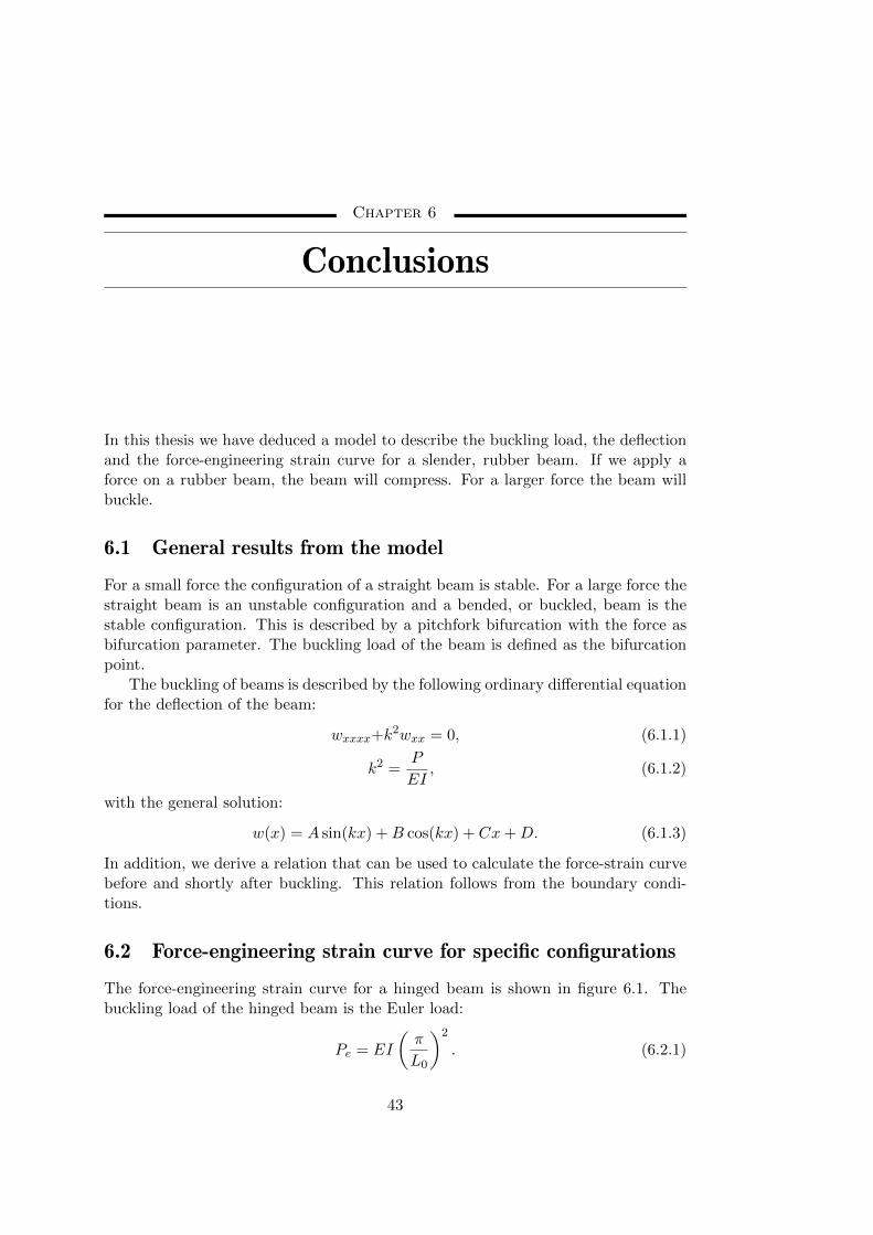
6.2 Force-engineering strain curve for specific configurations

The force-engineering strain curve for a hinged beam is shown in figure 6.1. Thebuckling load of the hinged beam is the Euler load:

Pe = EI

(π

L0

)2

. (6.2.1)

43

6.2. FORCE-ENGINEERING STRAIN CURVE FOR SPECIFIC CONFIGURATIONS

0 0.05 0.1 0.15∆lL0

P

((

∆lL0

)

c, Pc

)

Pe

Figure 6.1: The force-engineering strain curve of a hinged beam, where the green line isthe straight regime, and the blue one the buckled regime. The red point is the bucklingpoint and Pe is the Euler load of this beam.

If we scale the force with the Euler load we get the relative force. The slope of therelative force-engineering strain curve after buckling is equal to 2.

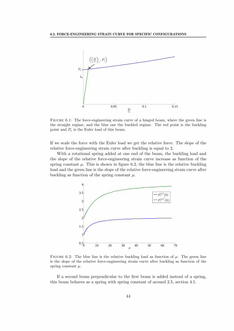
With a rotational spring added at one end of the beam, the buckling load andthe slope of the relative force-engineering strain curve increase as function of thespring constant µ. This is shown in figure 6.2, the blue line is the relative bucklingload and the green line is the slope of the relative force-engineering strain curve afterbuckling as function of the spring constant µ.

0 10 20 30 40 50 60 700.5

1

1.5

2

2.5

3

3.5

4

µ

P(µ)r (0)

P(µ)r

′

(0)

Figure 6.2: The blue line is the relative buckling load as function of µ. The green lineis the slope of the relative force-engineering strain curve after buckling as function of thespring constant µ.

If a second beam perpendicular to the first beam is added instead of a spring,this beam behaves as a spring with spring constant of around 2.5, section 4.1.

44

Appendix A

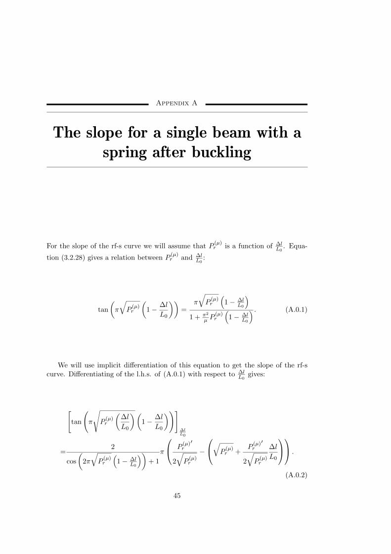
The slope for a single beam with aspring after buckling

For the slope of the rf-s curve we will assume that P(µ)r is a function of ∆l

L0. Equa-

tion (3.2.28) gives a relation between P(µ)r and ∆l

L0:

tan

(π

√P

(µ)r

(1− ∆l

L0

))=

π

√P

(µ)r

(1− ∆l

L0

)1 + π2

µ P(µ)r

(1− ∆l

L0

) . (A.0.1)

We will use implicit differentiation of this equation to get the slope of the rf-scurve. Differentiating of the l.h.s. of (A.0.1) with respect to ∆l

L0gives:

[tan

(π

√P

(µ)r

(∆l

L0

)(1− ∆l

L0

))]∆lL0

=2

cos

(2π

√P

(µ)r

(1− ∆l

L0

))+ 1

π

P(µ)r

′

2

√P

(µ)r

−

√P (µ)r +

P(µ)r

′

2

√P

(µ)r

∆l

L0

.

(A.0.2)

45

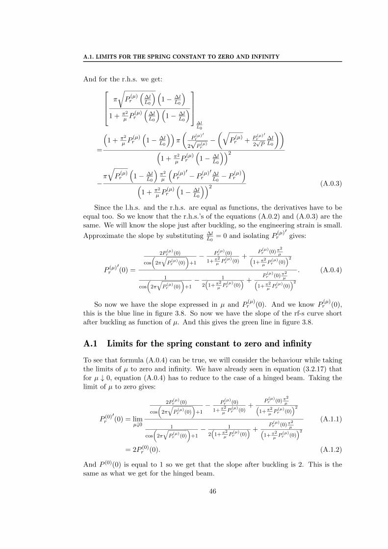
A.1. LIMITS FOR THE SPRING CONSTANT TO ZERO AND INFINITY

And for the r.h.s. we get: π

√P

(µ)r

(∆lL0

)(1− ∆l

L0

)1 + π2

µ P(µ)r

(∆lL0

)(1− ∆l

L0

)

∆lL0

=

(1 + π2

µ P(µ)r

(1− ∆l

L0

))π

(P

(µ)r

′

2√P

(µ)r

−(√

P(µ)r + P

(µ)r

′

2√P

∆lL0

))(

1 + π2

µ P(µ)r

(1− ∆l

L0

))2

−π

√P

(µ)r

(1− ∆l

L0

)π2

µ

(P

(µ)r

′− P (µ)

r

′∆lL0− P (µ)

r

)(

1 + π2

µ P(µ)r

(1− ∆l

L0

))2 (A.0.3)

Since the l.h.s. and the r.h.s. are equal as functions, the derivatives have to beequal too. So we know that the r.h.s.’s of the equations (A.0.2) and (A.0.3) are thesame. We will know the slope just after buckling, so the engineering strain is small.

Approximate the slope by substituting ∆lL0

= 0 and isolating P(µ)r

′gives:

P (µ)r

′(0) =

2P(µ)r (0)

cos

(2π

√P

(µ)r (0)

)+1− P

(µ)r (0)

1+π2

µP

(µ)r (0)

+P

(µ)r (0)π

2

µ(1+π2

µP

(µ)r (0)

)2

1

cos

(2π

√P

(µ)r (0)

)+1− 1

2(

1+π2

µP

(µ)r (0)

) +P

(µ)r (0)π

2

µ(1+π2

µP

(µ)r (0)

)2

. (A.0.4)

So now we have the slope expressed in µ and P(µ)r (0). And we know P

(µ)r (0),

this is the blue line in figure 3.8. So now we have the slope of the rf-s curve shortafter buckling as function of µ. And this gives the green line in figure 3.8.

A.1 Limits for the spring constant to zero and infinity

To see that formula (A.0.4) can be true, we will consider the behaviour while takingthe limits of µ to zero and infinity. We have already seen in equation (3.2.17) thatfor µ ↓ 0, equation (A.0.4) has to reduce to the case of a hinged beam. Taking thelimit of µ to zero gives:

P (0)r

′(0) = lim

µ↓0

2P(µ)r (0)

cos

(2π

√P

(µ)r (0)

)+1− P

(µ)r (0)

1+π2

µP

(µ)r (0)

+P

(µ)r (0)π

2

µ(1+π2

µP

(µ)r (0)

)2

1

cos

(2π

√P

(µ)r (0)

)+1− 1

2(

1+π2

µP

(µ)r (0)

) +P

(µ)r (0)π

2

µ(1+π2

µP

(µ)r (0)

)2

(A.1.1)

= 2P (0)r (0). (A.1.2)

And P (0)(0) is equal to 1 so we get that the slope after buckling is 2. This is thesame as what we get for the hinged beam.

46

CHAPTER A. THE SLOPE FOR A SINGLE BEAM WITH A SPRING AFTER BUCKLING

For the limit of µ to infinity we know that the the force only differs a factorof approximately 2.04 with respect to the hinged beam, see (3.2.27). So for thedifferentiation we get:

P (∞)r

′(0) =

[(C

π

)2

P hingedr

]′(0) (A.1.3)

=

(C

π

)2

P hingedr

′(0) = 2

(C

π

)2

. (A.1.4)

And for P(∞)r (0) we have:

P (∞)r (0) =

(C

π

)2

P hingedr (0) =

(C

π

)2

. (A.1.5)

And so the slope is two times as large as the relative buckling load. And indeed, ifwe take the limit for µ→∞ we get:

P (∞)r

′(0) = lim

µ→∞

2P(µ)r (0)

cos

(2π

√P

(µ)r (0)

)+1− P

(µ)r (0)

1+π2

µP

(µ)r (0)

+P

(µ)r (0)π

2

µ(1+π2

µP

(µ)r (0)

)2

1

cos

(2π

√P

(µ)r (0)

)+1− 1

2(

1+π2

µP

(µ)r (0)

) +P

(µ)r (0)π

2

µ(1+π2

µP

(µ)r (0)

)2

(A.1.6)

= 2P (∞)r (0). (A.1.7)

47

A.1. LIMITS FOR THE SPRING CONSTANT TO ZERO AND INFINITY

48

Appendix B

List of notation used

Symbol Meaning Calculation

wwwwwwDimensions of the beam

L0 Inertial lengthL Compressed lengthl Distance between the two endsh Heightb Widthw Deflectionr Distance to the middle line of the beamA0 Cross-section (area) A0=h · bI Second moment of area I=

∫∫A0r2dA0

wwwwwwStrain∆LL0

Strain ∆LL0

=L0−LL0

∆lL0

Engineering strain ∆lL0

=L0−lL0(

∆lL0

)c

Critical engineering strain

ε Local strainεb Local strain caused by the bending εb=−rwxx

wwwwwwForces

N Normal forceP ForcePc Buckling load

Pe Euler load Pe=EI(πL0

)2

Pr Relative force Pr=PPe

σ Stress σ= NA0− Erwxx

M Moment M=EIwxxwwwwwwGeneral

E Young’s modulus E= NA0

/∆LL0

µ spring constant µ= µL0

EI

49

Bibliography

[BC10] Zdenek P Bazant and Luigi Cedolin. Stability of structures: elastic, inelastic,fracture and damage theories. World Scientific Publishing Company, 2010.

[TG70] SP Timoshenko and JN Goodier. Theory of elasticity 3rd edition, 1970.

51

Buckling of a Beam - Universiteit Leiden

Documents

Transcript of Buckling of a Beam - Universiteit Leiden