REPORT OF INVESTIGATION NO. 23 1954

STATE OF ILLINOIS

WILLIAM G. STRATTON, Governor

Bubbler System Instrumentation For

Water Level Measurement

by Gerald H. Nelson

DEPARTMENT OF REGISTRATION AND EDUCATION VERA M. BINKS, Director

STATE WATER SURVEY DIVISION A. M. BUSWELL, Chief

URBANA, ILLINOIS

(Printed by the authority of the State of Illinois)

REPORT OF INVESTIGATION NO. 23 1954

STATE OF ILLINOIS

WILLIAM G. STRATTON, Governor

Bubbler System Instrumentation For

Water Level Measurement

by

Gerald H. Nelson

DEPARTMENT OF REGISTRATION AND EDUCATION VERA M. BINKS, Director

STATE WATER SURVEY DIVISION A. M. BUSWELL, Chief

URBANA, ILLINOIS

(Printed by the authority of the State of Illinois)

TABLE OF CONTENTS

Page ABSTRACT 1

ACKNOWLEDGMENT 1

INTRODUCTION 2

BUBBLER SYSTEM 4

Introduction and Description of Basic Components 4 Discussion of General Principle of Operation 4 Laboratory Studies for Development of Adapted Bubbler System 6

Flow Control 6 Equipment and Procedure 7 Results 8

Evaluation of Effective Bubble Pressure 9 Equipment and Procedure 9 Results .. 10

Frictional and Deformational Characteristics of Plastic Airline Tubing 10 Equipment and Procedure . 11 Results 11

Laboratory and Field Studies on Adapted Bubbler System 13 Description of Equipment Developed 13

Static Accuracy Tests 13

Equipment and Procedure 15 Analysis of Data 15 Results 16

Field Test 17 Equipment and Procedure 17 Analysis of Data 17 Results 20

Laboratory Tests of Field Methods of Water Level Measurement 20

Procedure 20 Results 20

CONCLUSIONS AND RECOMMENDATIONS 21 APPENDIX I: Calculation of Approximate Data Corrections 23

Assumptions 23 Required Data 23

Typical Data: Field Setup 23 Typical Data: Laboratory Setup.. 23

Correction of Field Data 23

(B + C) (WCO 2 ) : The Pressure Exerted by Vertical Column of CO2 in the Airline .. 23

Assumptions 23 Procedure and Example 23

hL: Airline Frictional Head Loss 25

Assumptions 25 Procedure and Example 25

B(wa i r): Pressure Exerted by a Vertical Column of Air in the Casing Be­tween the Datum and the Water Surface 26

Assumptions 26 Procedure and Example 26

Pb: Effective Bubbler Pressure 26 Summary 26

Correction of Laboratory Data 26

(D + E) (wCO2): Pressure Exerted by a Vertical Column of CO2 in the Airline 26

Assumptions 26 Example 27

hL: Frictional Head Loss 27

Assumptions 27 Example 27

(D + F) (wCO2): Pressure Exerted by Vertical Column of CO2 in the Pres­sure line 27

Assumptions 27 Example 27

Pb: Effective Bubble Pressure 27 Summary 27

APPENDIX II: Other Sources of Bubbler System Error 28

APPENDIX III: List of Symbols 30

1

ABSTRACT

To meet the frequent needs of engineers of the Illinois State Water Survey for a portable automatic water-level measuring instrument, a method for precise measurement of water levels in observation wells, utilizing bubbler system instrumentation, has been developed for well production tests. Since no summary of the possible sources of error in bubbler systems was found in the literature, these were investigated and the various forces affecting the accuracy of bubbler systems are discussed in this report.

The material presented herein may be adapted to develop instrumentation for measuring liquid levels (or specific weights) for a number of industrial, chemical or hydrologic applications where basic data-gathering accuracy is of primary importance. A procedure based

This Report of Investigation describes all significant research work and derived results from a project carried out by the staff of the Illinois State Water Survey Division's Hydraulic Laboratory Section pursuant to a request from the Groundwater Section. Laboratory work on this project was done under the supervision of H. E. Hudson, Jr., Head of the Engineering Subdivision. A preliminary exploration of the problem was carried on by R. E. Roberts in the summer of 1952. The author

on approximate formulas derived from hydrostatics was worked out for computing the required corrections to bubbler system data. Other field methods of water level measurement used by Survey engineers for production-test, water-level measurement were also checked to determine the accuracy obtainable. A laboratory com­parison of bubbler system instrumentation with methods now in use showed the measurement errors, using the bubbler system, to be one-fourth to one-tenth those obtained with the usual field measuring devices. Field trial of the bubbler system gave favorable results. The linear accuracy of bubbler system data analyzed by the equations presented herein was found to be almost entire­ly dependent upon the accuracy of the pressure - indicating device used to measure airline pressure.

wishes to acknowledge the contributions of Donald H. Schnepper, Professor V. T. Chow, and Professor J. C. Guillou, members of the University of Illinois Civil Engineering Department and also J. C. Buchta and Dr. Max Suter for technical review of this report and many valuable suggestions. Mr. G. A. Flom and Mrs. J. L. Abu-Lughod drafted the figures which appear in this report and Ray A. Schuster assisted with the editorial work.

ACKNOWLEDGMENT

2

INTRODUCTION

Since 1895, the Illinois State Water Survey has pro­vided services and conducted research for the citizens of the State of Illinois. The Groundwater Section of the Survey's Engineering Subdivision has, as one of its functions, the responsibility to encourage and observe pumping tests on municipal and private water wells in the state. Over 1300 pumping tests have been com­pleted to date under the direction of the Survey.

The data taken during these pumping tests are an­alyzed by the Survey staff and sent to the engineer in­volved, to waterworks personnel and the State Depart­ment of Health, so that they may readily determine the yield potential of the aquifer tested. Except for state-owned property, the Survey does not evaluate the data for the well owner; rather it provides aid in securing the basic data and presenting it in a form that may be easily used by the engineer in charge, who is acquainted with the immediate problems on location.

A pumping test is the everyday name for a "well production test." When a new well has been drilled for a municipality, city officials are naturally interested in knowing how good the well is. This knowledge is neces­sary to determine what size pump will be required, where to set the bowls, and what to expect in the way of long­

time yield from the water-producing formation. A pump­ing test is usually conducted to secure data to help answer these questions.

A pump is temporarily set in place. Preferably, pump­ing is continued at a constant rate for several hours, pos­sibly even three or four days, depending on the case. The discharge from the well is maintained at a constant rate, usually by a valve-orifice arrangement, and the distance to water is recorded at known times throughout the test. The difference between the non-pumping level and the pumping level is called the drawdown.

Notice in Figure 1 that a simple bubbler system is being used to measure the water level in the pumped well. The hand pump forces air down through the airline. The air under pressure displaces water that would nor­mally fill the airline. As water is displaced, the pressure

. increases until air bubbles out of the bottom of the air­line. -A gage with a scale of pressure values marked off in "ft of water" may be used to measure airline pres­sure. The maximum reading on the pressure gage indi­cates to a first approximation the "head of water" over the bottom of the airline. If the length of the airline is known, the distance from the top of the casing to the water level may be determined by subtraction. This type

FIG. 1- TYPICAL FIELD SETUP FOR WELL PRODUCTION TEST USING MANUAL BUBBLER SYSTEM IN PUMPED WELL.

3

of water level measurement instrumentation came into general use about 1930. It frequently forms part of the permanent installation in the well and gives readings that are usually of reasonable accuracy.

When sufficient clearance exists around the pump column pipe or when levels are being observed in an open observation well, other methods are frequently used. Their principles of operation may be classified into three main divisions: (1) electrical, (2) direct, and (3) float.

1. All electrical methods require an electrical cir­cuit which is activated by contact of a probe with water which contains dissolved minerals. The presence of dis­solved minerals between two contact points makes the well water a semi-conductant and a galvanometer or light circuit is activated when the probe touches the wa­ter. Examples of this method are battery-powered single and double-wire drop lines. A recent advancement in electrical water level measurement is the electrolytic or self-activating method. A short rod of magnesium is fixed to the end of a steel tape orwatertight lightweight con­duit. When the rod touches the water, current flows through a galvanometer to indicate the presence of a completed circuit.

2. The direct methods may use a weighted steel tape with water-level-indicating compound, a long graduated wooden pole, or even a weighted chalk line.

3. Frequently, floats are also used to indicate water levels. They are usually used in conjunction with re­corders. If a recorder is not available or if extreme ac­curacy is not important, a float is sometimes fastened to a steel tape or marked line to accomplish the same purpose.

There are several other methods for measuring water levels, such as float or probe-activated sensing and sonic devices, which will not be discussed here. The methods previously mentioned are the most used at present. It would seem logical to determine the usefulness of the "old standby" methods before resorting to additional refinements.

An examination of the literature failed to disclose any study of the precision to be expected from various methods of water level measurements. The airline method for use in wells is given in a number of publica­tions as an approximate method for determining water level. The continuous gas-purge bubbler method for water level determination is described in standard engineering reference publications, and there is an ex­tensive commercial literature on the subject. However none of the published information on continuous gas-purge liquid-level measurement methods summed up the possible sources of error in bubbler systems using continuous gas flow.

A program was therefore set up to study water level measurement methods for pumping tests. Methods and equipment currently used by the State Water Survey were studied. Considerable time was spent on the development of bubbler system instrumentation, since its principle of operation is not readily apparent. One of the final objectives of the study was to determine the magnitude of error to be expected with a given method while measuring the distance to a static or

very slowly moving level. From a practical standpoint it would be desirable, upon the conclusion of this study, to be able to write accuracy specifications for water-level measuring devices for use in the field for produc­tion tests. It then would be possible to compare the accuracy of a given method, as determined by lab­oratory tests, with these specifications and judge the method's usefulness. This is very difficult for a number of reasons.

For example, it would be desirable to state that the water level measuring device must indicate the true level to within, say 0.5 per cent (this figure is for ex­planation only) of the linear value of the maximum drawdown. This, in effect, makes the linear value of allowable error dependent upon the drawdown. The drawdown value may range between two or three inches for remote observation wells to several hundred feet for a pumped well drilled in bedrock. One of the main purposes of a production test is to determine how much drawdown results from a given pumping rate. Therefore, it is impossible to know beforehand how much drawdown will result. The engineer conducting the test is there­fore faced with the unique problem of not knowing what linear accuracy he needs until he is through with his work. For reasons of economy, production tests are usually conducted only once.

Another way to write the specifications would be to state that the method under consideration must be more accurate than any we have at present. This is ambiguous since portability, self-recording features, and economy must be considered, in addition to precision. Accuracy is one of the factors that can be evaluated readily by laboratory tests and error analysis. This was done for Survey-owned instruments and the results are presented in Table 2. These results do not fully indicate the useful­ness of the instruments tested since other features (economy, portability, etc.) do not show in these figures.

A temporary "rule of thumb" standard has been set up by the Groundwater Engineers of the Survey. Their desire is to be able to read the scale of the indicating or recording device to the nearest 0.01 ft. In a majority of the field tests conducted, linear error values of 0.03 to 0.05 ft would have an indistinguishable effect on the analysis of the results.

Occasionally, however, engineers are called upon to measure water levels in small diameter observation holes located a great distance from the pumped well. Water levels in such wells recede less than two feet as a result of test pumping programs, and an error of 0.01 feet would be smaller than occurs with conventional field engineering equipment. Such an error would amount to 1 part in 200, which conies within the usual specifica­tions of high-quality pressure-indicating instruments. More precision than 0.01 feet does not seem to be warranted by the analytical techniques available for correlating the data. Other factors that cause minor variances, such as barometric effects, require the ap­plication of corrections which are not to be trusted for a precision greater than 0.01 feet. It was therefore sought to develop bubbler system instrumentation to the point where it is theoretically possible to obtain the maximum linear error of 0.01 feet.

4

BUBBLER SYSTEM

Introduction and Description of Basic Components

Although industrial concerns may use direct or elec­trical methods for measuring liquid levels, they have found bubbler system (or air-purge) instrumentation advantageous when liquid level measurements must be taken from many scattered storage tanks. An industrial application of the bubbler system method is shown in Figure 2.

FIG. 2-INDUSTRIAL APPLICATION OF BUBBLER SYSTEM INSTRU-MENTATION TO MEASURE TANK LEVELS.

As may be noted from Figure 2, three components are necessary for a bubbler system setup: (1) a flow con­trol device, (2) an instrument to measure pressure, and (3) an airline and instrument tubing. The flow control device is merely a metering device which can maintain a known rate of gas flow down the airline. When the bottom of the airline can be observed, the rate of flow is usually adjusted so that ten to fifteen bubbles form per minute. A pressure-sensing instrument is required to indicate the airline pressure. Air is commonly used to purge the liquid out of the airline. Obviously, the gage pressure at the airline nozzle is due to the hydrostatic head of liquid above this elevation. If the pressure dif­ference between the nozzle elevation and the recorder is negligible, the pressure recorder or gage reading is a measure of the water level above the bottom of the airline. The pressure recorder may be located on the control panel of the instrument room along with other similar instruments and the operator can tell at a glance what is going on in his section of the plant.

This method may also be used to determine the density or specific gravity of liquid chemicals during their manufacture. In this case, as shown in Figure 3, two airlines are used. The pressure recorder actually registers the difference in pressure between two levels but may also record the specific gravity of the fluid if the scale is graduated properly. The Peoria Laboratory Subdivision of the Survey is now using a modified bubbler system to measure liquid levels in two head tanks connected to a venturi meter that meters silt-laden raw river water. Besides these applications, the system has also been used to measure liquid levels in tanks, sewer lines, rivers, etc.

The above description of a basic bubbler system ap­plication is rather simplified. This simplification is justified when small changes of level are to be measured.

If large ranges are to be measured the factors causing the discrepancy between observed and true values should be investigated to correct the pressure recorder reading so that a reasonable linear value of error is realized.

The figures and diagrams used in the remainder of this report, as well as the examples cited, will be con­cerned with the immediate problem of measuring water levels in wells. The subject matter is general however, and can be applied to any situation desired.

Discussion of General Principle of Operation

In order to clarify some of the factors, not readily apparent, which affect the accuracy of the bubbler system, a field setup using carbon dioxide as the purge gas is illustrated in Figure 4. Two parts of the equip­ment shown are not commonly used and are described in detail later: the electromagnet to hold the bubbler nozzle against the steel casing at a given elevation, and the carbon dioxide bottled gas cylinder and pressure reducer. However, these modifications do not affect the general principle of operation.

FIG. 3-INDUSTRIAL APPLICATION OF BUBBLER SYSTEM INSTRU­MENTATION TO MEASURE SPECIFIC GRAVITY.

Assuming static conditions of water level, a manom­eter type equation of pressures may be devised involving the known and unknown parameters:

Where: Pa = atmospheric pressure,

A, B, and C are distances measured in feet,

A and (B + C) are known, (used in conjunction with F igure 4 and the analysis of field data),

(wa i r) = specific weight of air in lbs/ft3 at known atmospheric pressure and tem­perature conditions,

(wH2O) = actual specific weight of water at a known temperature in lb/ft,3

(wCO2) = specific weight of carbon dioxide gas

under known temperature andpressure conditions expressed in lb/ft,3

Pb = the effective pressure required to make a bubble form and break away at the nozzle elevation (expressed in ft of water),

hL = frictional head loss in the airline ex­pressed in ft of water, and

Pr = pressure recorder reading in ft of water.

Equation 1 may be derived from well-known prin­ciples of hydrostatics. It is necessary to assume an arbitrary sign convention such as: (+) when the pres­sure is increased in the direction of travel around the bubbler system circuit and ( - ) when the pressure is decreasing in the direction of travel. The pressure at the datum is atmospheric (Pa). The pressure at the water surface inside the well is [ P a + B(w a i r ) ] . The pressure in the water at the bubbler nozzle is [P a + B(wair) + C(wH2O) ]. The remaining terms in Equation (1) may be written in a similar manner by moving up the airline to the pressure recorder and finally back to the datum. By canceling Pa and assuming A = 0 (the pressure recorder

5

FIG. 4-SCHEMATIC OF FIELD SETUP USING ADAPTED BUBBLER SYSTEM.

6

is usually situated at the datum), it is possible to solve for C(wH2O) directly:

From equation (2) it is possible to solve for the sub­mergence of the nozzle (C) by either multiplying the entire equation by 1/(wH2O) or by originally expressing all pressures in "ft of water." Therefore, if C can be calculated, the distance from the datum to the water level may be found by subtracting C from the known (B + C) measurement. Since the elevation of the top of the casing is known, the elevation of the water in the well can be determined directly by subtraction. The problem then reduces to the evaluation of unknowns in Equation (2). As a first approximation, the unknown C (in ft) may be assumed to equal the pressure recorder reading expressed in ft of water if the magnitude of the other corrections is small percentage-wise. This as­sumption gives us a means of calculating the unknown terms in Equation (2) to their first approximation. For convenience all values in Equation (2) except the pres­sure recorder reading P r and C ( W H 2 O ) have been termed corrections.

The B(wair) correction may be calculated from pro­cedures outline in Appendix I and the Pb, correction will be explained in detail later (Page 9). However, the hL, and (B + C) (wCO2) corrections need further con­sideration at this t ime. According to Kemler,1 the latter corrections are interrelated if the airline flow is con­sidered from a theoretical standpoint.

If we consider flow down the airline starting at the pressure recorder junction and assume isothermal flow and negligible kinetic energy:

where dL is an increment of length measured down the airline,

dh = total head loss over this increment,

V = velocity through increment or velocity of flow in ft/sec,

f = Darcy-Weisbach friction factor for increment, and

d = airline diameter in ft. This differential equation cannot be integrated directly since V, the velocity, is also a variable. However, it is possible1 to separate it and by suitable substitution and integration obtain:

1Kemler, E. A., "A Study of the Data on the Flow of Fluids in P i p e s , " Trans. A.S.M.E., Hydraulics Division, Vol. 55, No. 10, August 31 , 1933, p. 20.

e = base of natural logarithms, 2.718 . . . ,

a = airline cross-sectional area, in ft2,

P1 = pressure at top of airline, in lb/ft2 ,

P2 = pressure at nozzle, in lb/ft2,

w1 = specific weight of the gas at the top of the airline in lb/ft3,

W = flow rate of gas in lbs/sec,

g = local acceleration of gravity in English units,

L = length of the airline in ft, and

µ= absolute or dynamic viscosity of the purge gas at a known temperature.

As shown in its simplest form, Equation (4) is difficult to solve for P2 and is only as correct as the assumptions used in its derivation. Neglecting kinetic energy is a reasonable assumption. For example, the maximum air­line velocity head encountered in this study (CO2 gas at a maximum flow rate of 6.45 x 10 - 6 lbs/sec, atmos­pheric airline pressure and airline diameter of 0.01077 ft) equalled about 1.1 x 10 - 6 ft of water. Equation (4) was derived for a straight vertical airline and its accuracy is also almost entirely dependent upon the constancy of both C1 and C 2 . These conditions are usually not found in the field. In an attempt to obtain a workable correc­tion formula, it was decided to assume that the velocity term in Equation (3) was, for all practical purposes, a constant. Then it would be possible to integrate directly. Laboratory tests, which are described later, established that highly satisfactory results could be obtained by calculating hL and (B + C) (wCO2), separately, instead of using Equation (4). Methods for the calculation of these corrections are presented in Appendix I.

One more correction must be evaluated before Equa­tion (2) can be solved for C(WH 2 O)- This correction is Pb, the effective bubble pressure. Laboratory tests (de­scribed below) were conducted to evaluate this unknown, empirically, for the particular nozzle shape used.

Laboratory Studies for Development of Adapted Bubbler System

Flow Control

To evaluate the hL correction, the flow rate must be known. Three different types of commercial flow-control devices were secured and tested. In addition, two glass capillary tubes were constructed and tested.

7

Equipment ancPProcedure: The liquid displacement method is almost universally accepted as a standard of gas flow measurement.2 This method was employed in the calibration of the flow control devices tested. The con­struction and setup in the laboratory is shown in Figure 5. Using this device, the rates of flow under various dif­ferential pressure conditions, were measured.

FIG. 5 - LABORATORY SETUP OF GAS FLOW MEASUREMENT UNIT.

A schematic sketch of the essential components of this gas measurement calibration unit is shown in Figure 6.

FIG. 6-SCHEMATIC OF POSITIVE DISPLACEMENT METHOD OF GAS FLOW MEASUREMENT.

2Westmoreland, J. C., "Metering Gas F low" , Instrumentation, Vol. 6, No. 4, First Quarter 1953, p. 27.

To insure saturation, gas was allowed to bubble through the displacement liquid (water) for several hours prior to starting the tests. At the start of each test, valve A was opened and the storage tank was elevated, forcing the water level in the glass cylinder to rise above the top etch mark. Valve A was then closed, forcing gas to flow into the glass measurement cylinder. As the gas depressed the water level in the glass cylinder, the storage tank was lowered manually so that level 1 was maintained at the same elevation as level 2. The time required for level 2 to travel between the two etch marks on the glass cylinder was recorded. (This amounted to catching 0.031610 ft3 of the gas at atmospheric pres­sure in a known time.) Both gas temperature and barom­etric pressure were recorded during the calibration. The specific weight of the gas was computed from the ideal gas law, pv = nRT, and the calibration results were reported graphically.

Three types of commercial flow-regulating instru­ments and two glass capillaries were calibrated using the above method of gas measurement as the primary standard. The commercial instruments were individually mounted and levelled in position as shown in Figure 5. The discharge line from each of these instruments was connected to the intake of the gas measurement unit. The intake line pressure for the flow control instrument was maintained at a known pressure by a welding pres­sure regulator. Both air and carbon dioxide were used in the calibration of the commercial instruments.

Figure 7 shows a capillary tube constructed by "flame pulling" of one-quarter inch thick-walled glass tubing. A considerable amount of care was exercised in handling the capillary to avoid breakage during coiling. A brace between the two end sections was provided to add to the structural soundness. The capillary was then mounted inside a protective housing constructed of two-inch pipe fittings. The ends of the capillary were fitted with drilled-out plastic pipe bulkhead unions packed with string and non-hardening gasket material. A metal to glass joint was obtained which could stand 300 psi at a temperature of 120°F without leakage.

FIG. 7 - T Y P I C A L GLASS CAPILLARY TUBE.

The setup for calibration of these capillary tubes is shown in Figure 8. To the right of the box containing the carbon dioxide cylinder and regulators is a constant-temperature water bath. A mercury manometer is located directly in front of the bath. The gas flow liquid displacement meter is located in the background.

Figure 9, a sketch of the equipment, will aid in understanding its operation.

8

ratings and the actual flow rate were observed for all the equipment tested. This would be important if the flow-control devices were to be used for industrial ap­plication without initial calibration. All of the com­mercial devices tested have one feature in common-a valve for regulating flow. This valve is the main con­striction that causes a pressure loss. Because of the ex­tremely small rate of flow and nearly-closed setting, any tampering with this valve causes a high percentage change of actual flow. An attempt was made to elim­inate this objectionable feature by removing the valve handles and sealing the valve shafts so that they were tamper-proof. Even this did not prove satisfactory. The slightest amount of shock or temperature change of the packing caused a change in flow. Day to day variation in flow was found to be as much as ± 5 per cent with a fixed valve setting.

Since these instruments are calibrated to indicate air flow rates, the results of the tests with CO2 are not given here. The following table summarizes the results of the testing:

Maximum Range of Construction Rated Capac- Errors,

Instrument Material ity, scfh Per Cent

A Plastic 0.4 90-300 B Plastic 0.2 100-140

C Glass 0.2 0- 26

None of these instruments had linear relationships be­tween factory calibration and actual flow rate. In ad­dition, they were insensitive, so that it was extremely difficult to reproduce results with them. The above data represent averages of not less than four runs at each setting. Errors in use would therefore be larger than the figures given.

The results obtained by calibration of capillary tubes were much superior to those obtained with commercial flow-control devices. Capillary No. 1 was calibrated only for the range of temperature and pressure conditions expected in the laboratory. It was short in length, ap­proximately two inches, and the capillary was of very small diameter. This calibration was used in calculating hL for the static accuracy tests conducted in the lab­oratory. Capillary No.2 was calibrated for temperature and pressure conditions expected in the field. Its length of constriction was approximately 12 inches and it had a larger diameter than capillary No. 1. The more ex­tensive calibration of capillary No. 2 covered pressures from 40 to 100 psi differential and temperatures from 32° to 110°F.

Each plotted point on Figure 10 represents the aver­age of two sets of data taken at a known bath tempera­ture at different times during the day's run. As a further check, data were taken several days later at a pressure differential of 100 psi and at arbitrary bath temperatures. The deviation from the original calibration did not ex­ceed a one per cent error in flow rate.

FIG. 8-LABORATORY SETUP FOR THE CALIBRATION OF CAP­ILLARY TUBES 1 AND 2.

FIG. 9 - SCHEMATIC DIAGRAM OF EQUIPMENT USED FOR THE CALIBRATION OF GLASS CAPILLARY TUBES.

During the tests on both capillary tubes, the pressure regulator at the carbon dioxide cylinder was set at a measured constant value. Smaller capillary tubes were also constructed and placed in the discharge line down­stream from the main flow control capillary. These tubes were used only during the laboratory calibration tests and their only function was to impress a measured back pressure on the tube being calibrated. About five feet of plastic tubing was coiled in the bath upstream from the capillary being calibrated to insure equilibrium between bath and gas temperature.

Readings were taken on the mercury manometer, bath thermometer and liquid displacement meter, and the results, corrected for actual atmospheric pressure, were reported graphically.

For each of the two capillary tubes calibrated, read­ings were taken over a three-day period. High differen­tial pressure readings were taken the first day (see Figure 10), medium the second day, and low the third day. For each plotted point on the calibration curve, approximately one hour was required to bring the water bath to a desired constant temperature either by the addition of ice or hot water.

Results: Commercial flow-control devices made by three different manufacturers were calibrated. The re­sults with the commercial instruments tested were not encouraging. Deviations between the manufacturer's

9

FIG. 10-ESTIMATED ISOTHERMAL DISCHARGE CURVES FOR CAPILLARY NUMBER 2 WITH CO2 FLOW AND 100 PSI

ENTRANCE PRESSURE.

Although the time required to calibrate capillary tubes for a particular industrial or laboratory application seems prohibitive, the substantial increase in accuracy may be worth the cost involved when precise measure­ment and control of gas are required.

Evaluation of Effective Bubble Pressure The value of the Pb correction must be determined

before a solution of Equation (2) can be completed. For the purposes of this report, the "effective bubble pres­sure" is defined as a head loss that occurs as the gas flows out of the nozzle into the surrounding water in the form of bubbles. The main cause of this head loss is the work required to overcome surface tension during the formation of bubbles. This work (or energy) is lost as the bubble breaks away. Obviously, the energy to form bubbles must come from inside the airline. If this cor­rection were neglected, an excessive reading on the air­line pressure recorder would result.

The maximum value of Pb, may be calculated using standard reference marks such as that of Adam.3 For the nozzle shape and dimensions described in Figure 12 a calculation of maximum Pb was made assuming a zero contact angle and a "spherical" bubble shape. The calculated value lies between 0.009 and 0.010 ft of water.

3Adam, N, K., The Physics and Chemistry of Surfaces, Second Edition, Oxford University Press , England, 1938, Page 372.

Equipment and Procedure: The laboratory setup for evaluation of Pb is shown in Figure 11. Figure 12 is a sketch showing the essential parts of the equipment. A brass bubbler nozzle (identical to the one used in the static accuracy tests) was mounted under water in a pressurized glass jar. The distance (y) from the bubbler tip to the water surface was measured by sighting through the glass walls of the jar to a steel tape mounted on the nozzle. Well pressure was simulated by discharging gas down the laboratory well airline. Pressures between 0 and 40 ft of water could be maintained by regulating the level in the laboratory well (see Page 15). The pressure drop (h) across the jug was measured on the water ma­nometer, where h = y + Pb = losses. If losses are neg­lected, h = y + Pb. The velocity head through the tubing was calculated to be approximately 6.0 x 1 0 - 3 ft of CO2, using maximum discharge of capillary No. 1. Neg­lect of frictional losses was deemed expedient. Pb may therefore be calculated from the known y and h readings and the above formula.

FIG. 11 - LABORATORY SETUP FOR THE EVALUATION OF THE EFFECTIVE BUBBLE PRESSURE.

FIG. 12-DIAGRAM OF EQUIPMENT USED TO EVALUATE EFFEC­TIVE BUBBLE PRESSURE.

Laboratory tests demonstrated a fallacy in the above reasoning. Pb reached a maximum value an instant be­fore each bubble broke away from the nozzle and reached a corresponding minimum following the break. Maximum and minimum readings were therefore taken on the water manometer. As a separate and distinct run, several

10

photographs were taken at various discharge pressures to catch the bubble just before the break and measure its maximum size. Such a photograph isshown in Figure 13.

FIG. 13 - TYPICAL BUBBLE FORMATION: Discharge pressure 35.786 ft of H2O Maximum bubble pressure 0.016 ft of H2O Minimum bubble pressure 0.012 ft of H2O Maximum bubble height 0.012 ft

Results: As expected, the value of Pb varied with both time and pressure. The bubble pressure varied be­tween 0.012 and 0.016 ft of water. Its value depended on the size of the bubble at the particular instant of measurement. Maximum and minimum bubble pressure (in ft of H2O) and the maximum bubble height (ft) are plotted against the pressure at the bubble (analogous to the nozzle submergence) in Figure 14.

No exact theoretical analysis of results as shown in Figure 14 was attempted. However, the existence of a bubble pressure was substantiated for the conditions cited. The value of Pb for use in Equation (2) lay between 0.012 and 0.016 ft of water and may be dependent upon the rate of bubble formation. The use of an average value of 0.014 would be satisfactory if one considers the range of possible error (±0.002 ft of water) to be neg­ligible. A slightly better approximation could be ob­tained if the maximum bubble height curve is used to represent Pb. This was done for laboratory and field tests. Either procedure would be justified.

The observed value of the maximum bubble pressure of water does not agree well with the calculated values of 0.009-0.010 ft of water. The assumption of spherical

Pressure Variation due to Bubble Formation (ft.) FIG. 14 - RESULTS OF LABORATORY TESTS FOR EVALUATION OF

EFFECTIVE BUBBLE PRESSURE.

shape and zero wetting angle are certainly not fulfilled (see Figure 13). Therefore, results obtained from this calculation are not applicable in this case. The radius of the nozzle is much larger and of a different shape than is commonly used with this method to determine surface tension at a liquid-gas interface. The nozzle shape and size shown in Figure 12 are not a particularly suitable design even though they serve to demonstrate the principles involved. If the nozzle were ideally con­structed and if the water could always be of known purity, maximum bubble effect could be calculated from information contained in reference works on phys­ical chemistry.(3) NO attempt was made to evaluate the change in the value of Pb due to the effects of water temperature on surface tension, tipping of the bubbler nozzle, or changing flow rates. The accuracy of possible measurement did not appear to warrant such refinement. However, the laboratory tests established the magnitude of Pb, for the nozzle described. Its approximate effect will therefore be taken into account in the analysis of laboratory and field data.

Frictional and Deformational Characteristics of Plastic Airline Tubing

A limited study was initiated to investigate the fric­tional and deformational characteristics of a relatively new type of polyethylene instrument tubing now on the market. The description of the tests conducted and the results obtained are presented here as a service to organ­izations and laboratories who desire to extend this work.

11

The tests on the frictional characteristics reached a Reynolds Number of approximately 1.3 × 104: the max­imum value expected for field and laboratory tests on the adapted bubbler system with commercial flow con­trol. It was later decided that calibrated capillary tubes should be used as a more accurate means of flow control. This decision limited the flow entirely to the laminar range and the value of 64/R was used for the Darcy-Weisbach friction factor.

known temperature and reweighed. From the differen­tial weight and the known length, the average diameter was computed. Known pressures were applied to the water filled tubing. Scale readings were taken as soon as an apparent equilibrium condition was attained fol­lowing the addition of an increment of pressure, usually within one minute. The diameter was computed from the total differential weight, obtained by subtracting the scale reading at a given pressure from the zero pressure reading. The results are shown in Figure 15.

The frictional characteristics of the proposed airline tubing were investigated by use of the laboratory setup shown in Figure 16. One hundred feet of tubing was fastened to a horizontal supporting framework in the main laboratory area. Slanting piezometer leads were extended from the upstream to the downstream ends of the tubing, and the pressure differential, with a known flow of water, was measured with a mercury manometer. Friction factors were computed for the Darcy-Weisbach formula and plotted against Reynolds Number (R). The assumption of a constant diameter was made.

FIG. 16 - LABORATORY SETUP FOR THE EVALUATION OF FRIC­TIONAL CHARACTERISTIC OF PLASTIC AIRLINE TUBING.

Results: As may be noted from Figure 15, within the range of pressures impressed, the changes in diameter of the plastic tubing tested were negligible. Undoubtedly, actual field temperature and continuance of stress would affect deformation considerably. The laboratory tests were conducted merely to show the approximate effect of increasing pressures on the diameter. A percentage change of the magnitude encountered would have a negligible effect on the final calculated value of head loss. Therefore, the assumption of rigid pipe was made.

The results of the test to determine the frictional characteristics of the plastic tubing are shown in Fig­ure 17. Tests were conducted in the upper region of the laminar range as a further check on the equipment. The results obtained are almost identical to the expected theoretical curve, f = 64/R. A sharp break from laminar to turbulent flow occurred at a Reynolds Number of 2000, indicating the presence of some initial disturbing rough­ness. The portion of the transition range shown is char­acteristic of moderately smooth pipe, but this study

Percentage Change In Diameter FIG. 15-RELATION BETWEEN DIAMETER AND PRESSURE FOR

ONE-QUARTER INCH O.D. PLASTIC AIRLINE TUBING. The deformational tests were conducted for a pressure

range of 0 to 107 ft of water at a temperature of 80°F. This test was not intended to be complete. It was con­ducted merely to indicate the approximate effect of pressure on airline diameter, as a means of determining the suitability of the tubing for well airline material. If the percentage change in diameter is small, the use of an average diameter would be justified in future head loss calculations. If, however, the diameter changes significantly with pressure, exact calculation of the head loss correction would become extremely involved.

Equipment and Procedure: One hundred feet of new plastic tubing was used for the deformation tests. The tubing was first weighed dry on a triple-beam-balance (sensitivity - 0.1 gram) and then filled with water of

4Stevens, J. C, "Error in Float-Operated Dev ice s , " Data Book, Fourth Edition, p. 33.

FIG. 17 - FRICTIONAL CHARACTERISTICS OF PLASTIC AIRLINE TUBING.

13

would have to be extended to higher values of R for a complete analysis. The results as shown cover the ex­pected range of flow for one quarter inch O.D. plastic airline material.

Laboratory and Field Studies on Adapted Bubbler System

Description of the Equipment Developed

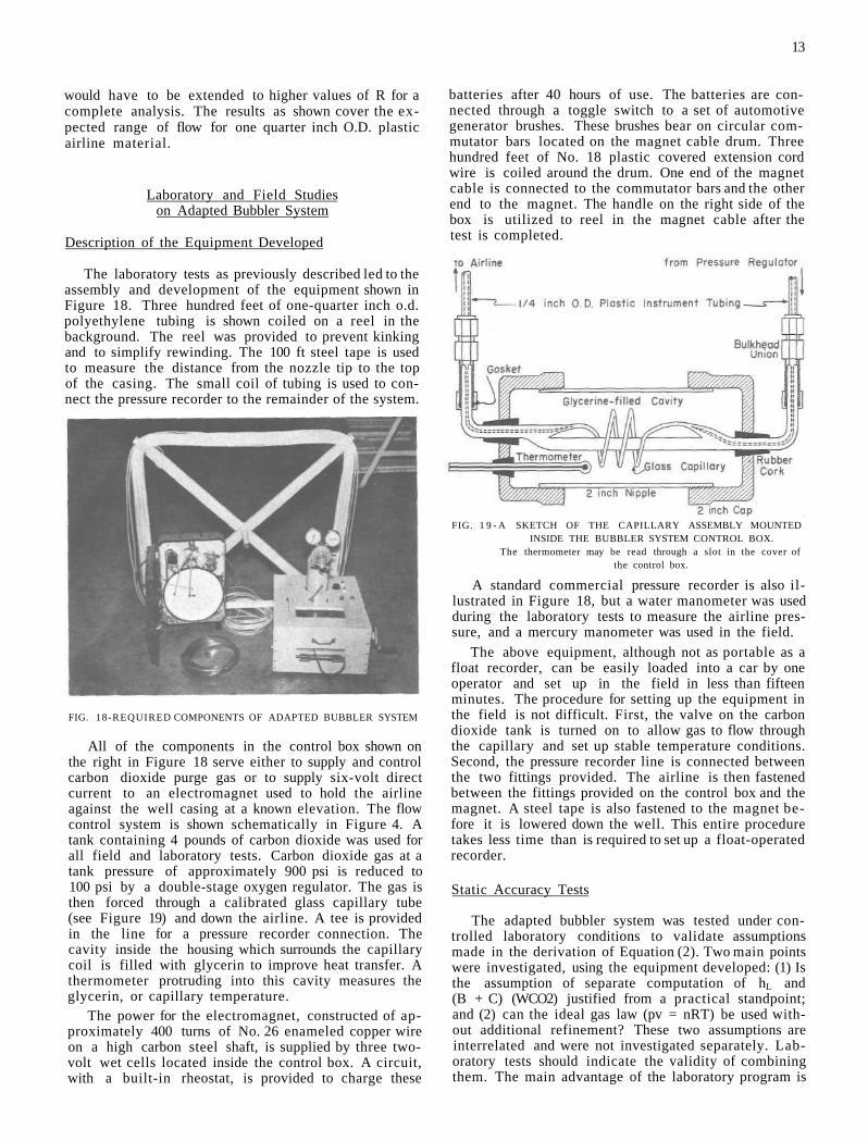
The laboratory tests as previously described led to the assembly and development of the equipment shown in Figure 18. Three hundred feet of one-quarter inch o.d. polyethylene tubing is shown coiled on a reel in the background. The reel was provided to prevent kinking and to simplify rewinding. The 100 ft steel tape is used to measure the distance from the nozzle tip to the top of the casing. The small coil of tubing is used to con­nect the pressure recorder to the remainder of the system.

FIG. 18-REQUIRED COMPONENTS OF ADAPTED BUBBLER SYSTEM

All of the components in the control box shown on the right in Figure 18 serve either to supply and control carbon dioxide purge gas or to supply six-volt direct current to an electromagnet used to hold the airline against the well casing at a known elevation. The flow control system is shown schematically in Figure 4. A tank containing 4 pounds of carbon dioxide was used for all field and laboratory tests. Carbon dioxide gas at a tank pressure of approximately 900 psi is reduced to 100 psi by a double-stage oxygen regulator. The gas is then forced through a calibrated glass capillary tube (see Figure 19) and down the airline. A tee is provided in the line for a pressure recorder connection. The cavity inside the housing which surrounds the capillary coil is filled with glycerin to improve heat transfer. A thermometer protruding into this cavity measures the glycerin, or capillary temperature.

The power for the electromagnet, constructed of ap­proximately 400 turns of No. 26 enameled copper wire on a high carbon steel shaft, is supplied by three two-volt wet cells located inside the control box. A circuit, with a built-in rheostat, is provided to charge these

batteries after 40 hours of use. The batteries are con­nected through a toggle switch to a set of automotive generator brushes. These brushes bear on circular com­mutator bars located on the magnet cable drum. Three hundred feet of No. 18 plastic covered extension cord wire is coiled around the drum. One end of the magnet cable is connected to the commutator bars and the other end to the magnet. The handle on the right side of the box is utilized to reel in the magnet cable after the test is completed.

FIG. 1 9 - A SKETCH OF THE CAPILLARY ASSEMBLY MOUNTED INSIDE THE BUBBLER SYSTEM CONTROL BOX.

The thermometer may be read through a slot in the cover of the control box.

A standard commercial pressure recorder is also il­lustrated in Figure 18, but a water manometer was used during the laboratory tests to measure the airline pres­sure, and a mercury manometer was used in the field.

The above equipment, although not as portable as a float recorder, can be easily loaded into a car by one operator and set up in the field in less than fifteen minutes. The procedure for setting up the equipment in the field is not difficult. First, the valve on the carbon dioxide tank is turned on to allow gas to flow through the capillary and set up stable temperature conditions. Second, the pressure recorder line is connected between the two fittings provided. The airline is then fastened between the fittings provided on the control box and the magnet. A steel tape is also fastened to the magnet be­fore it is lowered down the well. This entire procedure takes less time than is required to set up a float-operated recorder.

Static Accuracy Tests

The adapted bubbler system was tested under con­trolled laboratory conditions to validate assumptions made in the derivation of Equation (2). Two main points were investigated, using the equipment developed: (1) Is the assumption of separate computation of hL and (B + C) (WCO2) justified from a practical standpoint; and (2) can the ideal gas law (pv = nRT) be used with­out additional refinement? These two assumptions are interrelated and were not investigated separately. Lab­oratory tests should indicate the validity of combining them. The main advantage of the laboratory program is

14

15

the accurate measurement of the airline pressure and true water level (see Figure 20). The atmospheric-elevation correction, B(wair) was also eliminated from consideration. The chances of error in observation and calculation were substantially reduced by these pro­cedures.

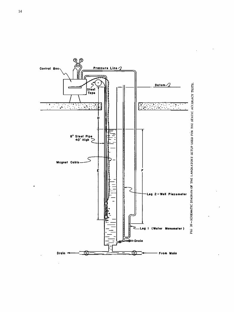
Equipment and Procedure: Figure 20 is a schematic diagram of the apparatus used for the laboratory tests. The laboratory well was constructed by joining two 20-ft lengths of eight-inch spiral weld pipe. The well was located in the hydraulic laboratory shaft which ex­tends vertically from the main laboratory area to the penthouse on top of the three-story Water Resources Building. The penthouse also contains a constant-head skimming-weir tank capable of handling 12,000 gpm.

The laboratory well was fitted with a piezometer to indicate the primary standard water level. This piezom­eter was constructed of three-eighths inch Tygon tubing mounted with a steel tape. A power hoist (3000 lbs ca­pacity) was fitted with a boatswain's chair to allow an observer to take readings over the entire 40-ft length of the piezometer. The method used in reading the well piezometer is shown in Figure 21.

The nozzle, with steel tape, airline, and magnet cable attached, was lowered into the well at the begin­ning of each test. When it reached the desired position, the magnet was activated, thereby maintaining a known elevation throughout the test. The distance (D + E) in Figure 20 was measured by a steel tape to ±0.002 ft. The steel tapes used for manometer and the airline were periodically checked with the University of Illinois' permanent post markers and temperature corrected for laboratory conditions.

Recommended tension was applied during the tests. The pressure line that would normally go to a pressure re­corder (see Figure 4 - field setup) was directed back down the laboratory shaft to the lower leg of a water manometer (Leg 1). The total maximum error in read­ing both legs of the water manometer was estimated to be ±0.003 ft.

The pressure regulator on the carbon dioxide jug was set at 46 psi, the value used in the calibration of capil­lary No. 1. Pertinent temperatures (see Table 1) were noted and recorded. Tests were conducted by recording levels indicated by Legs 1 and 2 of the water manometer as the laboratory well level was raised or lowered in approximately three-foot increments. Sufficient time, as determined by trials, was allowed before taking ma­nometer leg readings, to insure airline flow equilibrium. Once the operating characteristics and physical dimen­sions of the equipment had been substantiated, all the calculations for the analysis of data were based on read­ings taken on Legs 1 and 2, the measured distance (D + E), and laboratory temperature conditions.

Analysis of Data: The temperatures recorded during the static accuracy tests are given in Table 1. One test was conducted each day for six consecutive days. During this period the water used was unusually uniform in temperature.

FIG. 21-TAKING READINGSON LEG 2 OF THE LABORATORY WELL PIEZOMETER.

TABLE 1

Data Sheet

Number

Airline Temp.

°F

Pressure Line

Temp. °F

Capillary Temp.

°F

Well Water

Temp. °F

Airline Length

Number of Loops in Airline at Datum

36 37 39 40 41 42

80.0 77.0 78.0 77.0 76.4 80.7

80.0 74.0 78.0 77.0 76.4 80.0

80.0 77.0 79.4 76.5 76.8 82.5

55.0 55.0 55.0 55.0 55.0 55.0

200.0 200.0 50.0 50.0 50.0 50.0

15 30

None None None None

In order to analyse laboratory data, another equation similar to Equation (2) was written. Referring to Fig­ure 20, and again setting up an equation of pressures written from the datum down through the water to the bubbler nozzle, up the airline to the pressure line, down Leg 1 of the water manometer and finally up Leg 2 to the datum:

All of the above pressures may be expressed in feet of water by dividing Equation (5) by the specific weight of water. To find the resulting total error, the data were analysed by comparing the observed deviations

16

with the computed corrections

If the algebraic sum of the computed corrections was greater than the observed deviation for a given reading, the error (difference) was said to be negative, since the bubbler system would indicate a greater distance to water than actually occurred (the measured water level was below the true level). The converse would be true for positive errors.

The head loss (hL and (D + E) (WCO2) corrections were computed separately, rather than by Equation (4), which combines their effects. Methods and procedures for the calculation of all the computed corrections are given in Appendix I.

Results: The results derived from laboratory tests are presented in two parts: (1) results obtained with com­mercial instruments and procedures, and (2) results ob­tained with the adapted bubbler system.

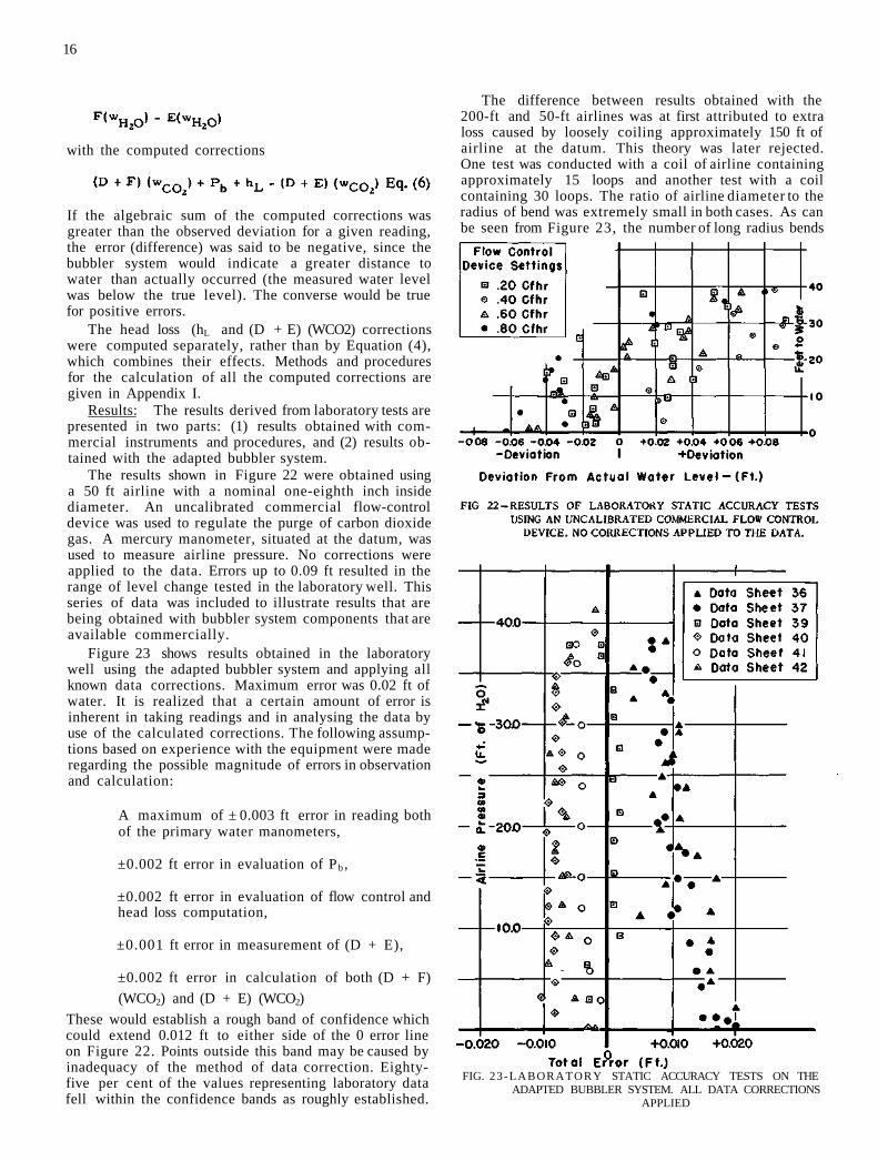
The results shown in Figure 22 were obtained using a 50 ft airline with a nominal one-eighth inch inside diameter. An uncalibrated commercial flow-control device was used to regulate the purge of carbon dioxide gas. A mercury manometer, situated at the datum, was used to measure airline pressure. No corrections were applied to the data. Errors up to 0.09 ft resulted in the range of level change tested in the laboratory well. This series of data was included to illustrate results that are being obtained with bubbler system components that are available commercially.

Figure 23 shows results obtained in the laboratory well using the adapted bubbler system and applying all known data corrections. Maximum error was 0.02 ft of water. It is realized that a certain amount of error is inherent in taking readings and in analysing the data by use of the calculated corrections. The following assump­tions based on experience with the equipment were made regarding the possible magnitude of errors in observation and calculation:

A maximum of ± 0.003 ft error in reading both of the primary water manometers,

±0.002 ft error in evaluation of Pb ,

±0.002 ft error in evaluation of flow control and head loss computation,

±0.001 ft error in measurement of (D + E),

±0.002 ft error in calculation of both (D + F) (WCO2) and (D + E) (WCO2)

These would establish a rough band of confidence which could extend 0.012 ft to either side of the 0 error line on Figure 22. Points outside this band may be caused by inadequacy of the method of data correction. Eighty-five per cent of the values representing laboratory data fell within the confidence bands as roughly established.

The difference between results obtained with the 200-ft and 50-ft airlines was at first attributed to extra loss caused by loosely coiling approximately 150 ft of airline at the datum. This theory was later rejected. One test was conducted with a coil of airline containing approximately 15 loops and another test with a coil containing 30 loops. The ratio of airline diameter to the radius of bend was extremely small in both cases. As can be seen from Figure 23, the number of long radius bends

FIG. 23-LABORATORY STATIC ACCURACY TESTS ON THE ADAPTED BUBBLER SYSTEM. ALL DATA CORRECTIONS

APPLIED

17

in the airline at the datum elevation did not seem to affect the results obtained with the 200-ft airline.

It appears that more accurate corrections were ob­tained when the airline pressure was high. This is in part evidenced by the tendency of plotted points to con­verge toward the ordinate at high airline pressures. To illustrate this, 100 per cent of the points fall within the confidence band when the airline pressure is above 25 ft of water. On the basis of these data, it is believed that if the adapted bubbler system (200-ft airline) and a pressure indicating device accurate to 0.010 ft of water were used to measure water levels during production tests, results to approximately ±0.020 ft of water could be expected.

Field Test

The initial object of the field test program was to verify assumptions made in the calculation of the B(wair) correction for Equation (2). This correction was purpose­ly eliminated from the laboratory setup. In order to validate completely the exactness of the correction, it would be necessary to measure airline pressures in the field as accurately as was done with the 40-ft laboratory water manometer. Obviously, this could not be accom­plished in the field. The best readily-available sub­stitute was a double-leg glass-tube mercury manometer. This manometer was constructed with an etched lucite slide so that the level of the top of the meniscus could be read on the manometer scale. No magnification was used, nor were parallox-preventing methods employed. The manometer scale was a steel tape graduated in feet and hundredths. The manometer was tested in the lab­oratory by comparing its indicated pressure with the pressure indicated by a 40-ft plastic tube water manom­eter. The mercury manometer readings were corrected for temperature and also for the pressure effect of a vertical column of air extending from the manometer to the top of the upper water level. An average error of 0.019 ft with a standard deviation of 0.022 ft resulted. By use of the laboratory data collected for the bubbler system with 200-ft airline and the results reported above for a separate test on the mercury manometer, a 0.031 ft mean error, 0.022 ft standard deviation, and a 0.067 ft, 95 per cent accuracy limit was computed for the com­bination. It was assumed that bubbler system and ma­nometer errors were independent. These computed values should then resemble results obtained by a field setup with the same equipment if the B(wair) correction is valid. In the field, unfortunately, primary standard measurements of the true water levels are not available. A float operated water stage recorder was used and the assumption was made that it indicated the true level. It was therefore impossible to obtain a precise check on the B(wair) correction, but field tests would indicate its approximate validity within the limits of error expected with the equipment used.

Equipment and Procedure: The bubbler system was tested under actual field conditions on an eight-inch observation well during a production test conducted at the village of Gridley, Illinois. An eight-inch pumped well (No. 3) located 826 ft from the observation well, had recently been constructed to augment the municipal

water supply. The observation well (No. 1) was located inside a brick waterworks building about 30 ft from another city well (No. 2). City well No. 2 was shut off six hours prior to and during the production test.

FIG. 2 4 - F I E L D SETUP OF THE ADAPTED BUBBLER SYSTEM AND FLOAT OPERATED RECORDER ON OBSERVATION WELL

NO. 1 DURING GRIDLEY PRODUCTION TEST.

The actual setup on observation well No. 1 is shown in Figure 24. The bubbler system setup may be sche­matically represented by Figure 4, except that a mer­cury manometer (not shown in Figure 24) was used to measure Pr. A temperature recorder with a gas-filled extension bulb was used to measure air temperature in the well 20 ft below the top of the casing. Water and well air temperatures were assumed equal to this in­dicated temperature. A Stevens Type F recorder with a four-inch copper float, beaded cable, and 12-hour time scale was also set up on the observation well to measure the water level. Times were measured by stopwatch and marked directly on the float recorder chart. Readings were taken on both legs of the bubbler-system mercury manometer, and capillary and room temperatures were read at definite times during both the recession and the recovery. A microbarograph was used to record barom­etric pressures during the test. The float-operated re­corder was "zeroed in" periodically during the test by steel tape with indicator compound. The distance to the bubbler nozzle was measured as described above by steel tape attached to it.

Analysis of Data: Uncorrected water level readings recorded during the Gridley test were first taken off the float-operated recorder charts to the nearest thousandth of a foot and corrected as suggested in the manufacturer's operational handbook.3 The situation under which the float recorder was operated must be considered. The handbook states that errors may be due to (1) float lag, (2) line shift, (3) submergence of the counterpoise, (4) temperature, and (5) humidity. For conditions at the Gridley test the original measurement by which the re­corder was "zeroed in" was another possible source of error.

(1) Float lag includes play between moving parts plus water level change required to start initial movement

18

of the instrument. If the recorder pen could be set on the true level during a rising stage, it would indicate true level (as far as the float lag correction is concerned) for all rising stages. (2) When the stage rises some of the line passes over the recorder pulley. This addition to the counterpoise side causes the float to ride higher out of the water. The correction is proportional to the amount of line that has passed over the pulley since the last true reading. The maximum line shift correction for the Gridley test amounted to 0.01 ft. (3) If the counterpoise becomes submerged the correction for line shift is af­fected. This condition did not exist during the Gridley test. (4) Changes in temperature affect the length of the float cable. Therefore, the temperature change must be known since the time of the last true reading. Well temperatures were unusually constant over the period of the production test. Well air temperature was recorded and found to be 53°F continually during the Gridley test. (5) Correction for the effect of humidity on the size of the recording paper was not considered. In a most ex­treme case the paper may expand or contract as much as two per cent. Readings of the true level must be known during the test to determine this effect unless special procedures and recording papers are used. Even then, this correction is usually negligible. Humidity changes at Gridley appeared to be very small.

In the above, the complete correction of float record­er data is primarily dependent upon at least one accurate measurement of the true distance from the datum to the water level in the well. The so-called true distance from the top of the casing to the water level in the well was measured with a steel tape. The tape had been pre­viously checked against permanent post markers. Water-level-indicating compound was used on the tape and the ten measurements of true level assumed were corrected for actual well air temperature. The data obtained from the float recorder cannot be more accurate than steel tape measurements of the true distance to water. It is not possible to determine how accurately each tape measurement was made in the field; however, a liberal estimate of error would be ±0.01 ft.

Bubbler system data taken during the Gridley test were analysed by application of Equation (2). The pro­cedure for calculating corrections is given in Appendix I. The manometer differential, in feet of mercury, was first converted to feet of water. The conversion factor for this process is the ratio of the specific weight of mer­cury to the specific weight of the well water. The tem­perature of the mercury and the well water must be known and used in determining both specific weights. The mercury temperature varied with time; therefore, the conversion factor also varied with time. A graph of the conversion factors was plotted as shown in Figure 25, based on room temperature data and tables5 of the spe­cific gravity of mercury and water at known tempera­ture. The value of Pb in Equation (2) was found by multiplying the feet of mercury differential by the ap­propriate conversion factor, obtained from Figure 25, at given times during the test.

The distance (B + C), measured by steel tape, was

5Lange, N. A., Handbook of Chemistry, Seventh Edition, Handbook Publishers Inc., Sandusky, Ohio, 1949, pp. 1385-1387.

FIG. 25-MANOMETER CONVERSION FACTORS FOR THE GRIDLEY TEST.

also temperature corrected to obtain the true distance. The data corrections were then calculated for known conditions at various times during both the recession and recovery. The results were algebraically summed and plotted against corresponding times. Figure 26 shows the summation of the corrections to be applied to all bubbler system data for this test.

The procedure of calculating only a sufficient number of data corrections to obtain a graph of the type shown in Figure 26 reduces considerably the number of calcula­tions required. Airline pressure or any other appropriate scale could be substituted for the abscissa of Figure 26, depending on the proposed use of the bubbler system. However, for water level measurement during production tests, the use of time as a scale for the correction graph is convenient, since it is one of the independent vari­ables of the test that can be readily and accurately measured without significant error.

FIG. 26-SUMMATION OF DATA CORRECTIONS FOR ANALYSIS OF BUBBLER SYSTEM DATA FOR THE GRIDLEY TEST.

For further simplicity when extreme accuracy is not required, perhaps only two or three points would have to be calculated and plotted to obtain an approximate cor­rection graph similar to the type shown in Figure 26. Another possibility, expedient in some cases, would be to "zero in" the bubbler system at the beginning of the test (as is done for float-operated recorders) and assume that the summation of the corrections remains constant. Under circumstances such as were present for the Gridley test, maximum error would have been 0.07 ft if this procedure were followed. One should be careful, how­ever, to obtain all data necessary for complete correction if a more detailed analysis is later required.

FIG. 27 - RESULTS OF PRODUCTION TEST AND COMPARISON OF DATA OBTAINED FROM ADAPTED BUBBLER SYSTEM AND FLOAT-OPERATED RECORDER.

20

Results: The final results of the field test program are shown in Figure 27. As can be observed, the dif­ference in results obtained with the float-recorder and the corrected bubbler system appeared indistinguishable. However, observation of a large-scale plotting of this graph, produced for analysis of field data, revealed cer­tain differences. Such a graph was used to compare data from both the corrected bubbler system and the float recorder. Readings of deviation (difference between the levels indicated by corrected float recorder and bubbler system, in feet at a given time) were taken from this graph for analysis. For this comparison, the float record­er was assumed to indicate the true level.

The magnitude and number of the deviations were then analysed statistically. A mean error (average error)

of 0.024 ft resulted between the bubbler system and the float-operated recorder. A standard deviation of 0.032 ft about the mean error and a 0.076 ft 95 per cent ac­curacy limit were also found." The above values com­pare favorably with results predicted by laboratory tests (see Table 2) for the bubbler system (200 ft airline) and the mercury manometer combination. The standard de­viation determined by field data was found to be larger than the laboratory value. This is reasonable since a float recorder with a certain amount of uncorrectable error was used as the primary standard in the field. The data indicate that, within the accuracy available in the field, the assumptions made for calculating B(wair) were satisfactory.

LABORATORY TESTS OF FIELD METHODS OF WATER LEVEL MEASUREMENT

Four field methods used by the Survey were tested in the laboratory well to determine the accuracy obtained in the field. Equipment for these four methods is illus­trated in Figure 28. The instruments were taken directly from field use and were not modified significantly. New markers were placed on the single-wire and double-wire drop lines as is routinely done before field use. There­fore, any stretching of the drop lines that occurred during the laboratory tests would also occur during field tests. The steel tapes were also taken directly from field serv­ice and were assumed to be true length. These procedures were followed to find the error actually resulting in the field with field equipment rather than to determine max­imum possible laboratory accuracy with equipment in perfect condition.

Procedure

The four field methods were tested in the 40-ft, eight-inch laboratory well previously described on page 44. Leg 2 of the well piezometer (Fig. 20) indicated the true primary standard water level in the well. The read­ing on the piezometer tape corresponding to the datum elevation (top of. casing) was determined by a surveyor's level to 0.001 ft. Measurements were taken of the dis­tance from the top of the casing to water using the above methods and different observers. The actual distance to water was computed by subtracting the Leg 2 reading from the tape reading which corresponds to the datum elevation. The true level was then compared with the level indicated by each method and the difference (error) was computed for each set of data.

Results

The results of the laboratory investigations, using the various methods of water level measurement, and also field results obtained with the bubbler system are pre­sented in Table 2. The numerical values of deviations (in ft) for water level readings taken with a given opera­tor and method were analysed statistically.6 Ninety-five per cent accuracy limits are listed in Table 2. These values mean that 95 per cent of the measurements taken in the field lay within the limit stated.

FIG. 28 - COMMON FIELD METHOD OF WATER LEVEL MEASURE­MENTS THAT WERE TESTED IN THE LABORATORY WELL.

6Bell, H. E., "Statist ical Estimation of Accuracy Limits for Various Methods of Measuring Water Levels in Wells", Hydraulic Laboratory Section, Unpublished Progress Report, Illinois State Water Survey Fi les , June 1953.

21

Method Mean Error (ft)

Standard Deviation

about Mean Error

(ft)

95% Accuracy

Limits (ft)

FIELD METHODS 0.041 0 0198 0.074 Single Wire Drop Line — Flat Brass Probe (all data combined) 0.035 0.0119 0 055

1st observer (3 runs) 0.029 0.0130 0.050

10-27-52 11- 7-52 11- 7-52

0.054 0.017 0.011

0.0196 0.0060 0 0084

0.086 0.027 0.025

2nd observer (2 runs) 0 031 0.0059 0.041

11- 7-52 11- 7-52

0.032 0.030

0 0059 0.0060

0.042 0.040

3rd observer (2 runs) 0.040 0.0111 0.058

10-31-52 10-31-52

0.042 0.033

0.0107 0.0118

0.060 0.055

4th observer 5th observer

0.038 0.045

0.0100 0.0188

0.054 0.076

Two Wire Drop Line-Sharp Interior Probe

1st observer 0.091 0.0418 0.160

CONCLUSIONS AND RECOMMENDATIONS

The various water level measurement methods tested in the laboratory well have been tabulated in Table 3 in order of decreasing accuracy. The bubbler system was found to be the most accurate method tested in the lab­oratory. However, it must be remembered that a more precise procedure was followed in measuring airline pressures in the laboratory than would be possible in the field. The laboratory tests with the bubbler system were conducted primarily to verify assumptions made in the derivation of the data correction formulas.

TABLE 3

Method 95 Per Cent Accuracy Limits (Ft). (All Lab­

oratory Data Combined)

1. Bubbler System 0.014 2. Single wire drop line 0.055 3. Steel tape with indicator compound 0.06,7 4 Steel tape with 4-inch float 0.105 5. Two-wire drop line—sharp interior probe. 0.160

The steel tape with 4-inch copper float method was found to be in considerable error. This was due to the inability of the operator to "feel" the weight of the tape and float and to judge the right tension to main­tain during a reading.

The two-wire drop line method was subject to me­chanical difficulties, and the results reported for it are probably not conclusive. The drop line wire stretched considerably due to its weight and the electrical probe

used seemed insensitive. The electrical connections were not waterproof, causing shorts and resultant untrue readings. Operators have reported that this also occurs in the field.

As noted from Table 2, the variation in 95 per cent accuracy limits between different observers using the same method was also investigated. Five different ob­servers measured water levels in the laboratory well with the single-wire drop line. Observers 1 and 5 were inexperienced with the use of the equipment. As addi­tional tests were conducted, they became more profi­cient with a resulting increase in accuracy. The remaining three observers were acquainted with the use of the equipment in the field. These three observers all attained about the same degree of accuracy. Statistical analysis indicated that the difference in error values found between operators using the same method was not significant when compared with the difference in error values found between different methods.6

Every attempt was made during the laboratory tests of the field methods to duplicate field conditions and procedure. Observers who were familiar with the field use of the equipment conducted the tests in the lab­oratory following their own particular procedure. In general, the tests in the laboratory indicated a greater degree of inaccuracy than had been expected. Most of the error is believed to lie not with the equipment, but with the way in which it was used. A method such as the adapted bubbler system could eliminate many chances

TABLE 2 - ACCURACY LIMITS FOR THE VARIOUS METHODS

Method Mean Error (ft)

Standard Deviation

about ' Mean Error

(ft)

95% Accuracy

Limits <ft)

Steel Tape with Float

1st observer 0.053 0.0314 0.105 Steel Tape with

Indicator Compound

2nd observer 0.023 0.0267 0.067

MERCURY MANOMETER 0.019 0.022 0.055 BUBBLER SYSTEM

(All laboratory data) 0.008 0.0035 0 014 200 ft airline 0 012 0.0041 0.018

50 ft airline 0.006 0.0031 0.011

*BUBBLER SYSTEM

(200 ft airline) and Mercury Manometer (Laboratory) 0.031 0.022 0 067

BUBBLER SYSTEM

(200 ft airline) and Mercury Manometer (Field) 0.024 0.032 0.076

* Computed values by assumption of independence of manometer and bubbler system (200 ft airline) errors.

22

for observational error and would be advantageous in this respect.

The results obtained in the field with the adapted bubbler system were found to be comparable in accuracy to those obtained with a float-operated recorder, even though a mercury manometer, with inherent inaccuracy (see Table 2) was used to indicate airline pressure. At this time, the possible accuracy of bubbler-system in­strumentation to measure water levels during production tests appears to be almost entirely dependent upon the means used to measure or record airline pressures.

One important purpose of this paper is to point out and investigate the considerations that are important for accurate measurement of levels utilizing bubbler system instrumentation. Such a method has definite application for measuring water levels in small diameter or ob­structed test hole observation wells. The time consumed in evaluating the pressure corrections seems great, but the effort may be justified if a high degree of precision is required.

The work completed to date (1954) and described by this paper has been guided so that the results are most applicable and useful to groundwater engineers of the State Water Survey Division. This, however, does not preclude the use of this information for other applica­

tions. For example, the same procedures would also apply to the design and data correction of bubbler-system stream-gaging installations. The author believes that such a method of water level measurement could be used extensively in stream-gaging work for several reasons. The level changes to be measured are generally small and do not fluctuate rapidly. It might then be possible to use a high-grade non-portable commercial pressure recorder which could attain the necessary ac­curacy. The gas flow rate could be cut down consider­ably to make monthly or even less frequent maintenance possible. One disadvantage would be the additional office time required to correct the basic data, but this disadvantage might be overcome in at least three ways: (1) the simplest solution would be to omit correcting the data if the station could be designed so that errors would compensate; (2) a set of standard correction graphs could be worked up, or (3) precautions could be taken to design the scales of the recording instruments so that the data would be precorrected. Obviously, the one big advantage of bubbler system instrumentation for stream-gaging would be economy in initial construction. Ex­pensive still-well structures for float operated recorders would not be required. The difficulties occurring in the operating of still wells and connections to the stream would also be eliminated.

23

APPENDIX I

This Appendix deals with the detailed computation of corrections for bubbler system data. The assumptions preparatory to calculation are listed for clarity and an illustrative example is given for the calculation of each correction. In each of the parts of this Appendix which deals with the calculation of an individual data correc­tion, a series of letters follows a paragraph of heading entitled "Assumptions." Each of these letters refers to a corresponding assumption in the following master list.

Assumptions

A. Kinetic energy of flow is negligible.

B. The variation of pressure along the airline is small enough that the specific weight of gas may be assumed constant.

C. The airline pressure for the determination of the specific weight of the gas in the airline is equal to the pressure recorder or gage reading. (For analysis of field data.)

D. The airline pressure for the determination of the specific weight of the gas in the airline is equal to submergence of the nozzle. (For analysis of laboratory data.)

E. The temperature of the gas inside the airline is equal to the temperature of the surrounding air or water.

F. The temperature of the gas inside the pressure line is equal to the laboratory air temperature. (For analysis of laboratory data.)

G. pv = nRT

H. The frictional head loss value calculated for a known length of straight horizontal airline is ap­plicable to the same length of vertical airlines.

I. A change in atmospheric pressure has a negli­gible effect on the calibration of the flow control device.

J . The pressure gage or recorder is located at the datum elevation.

K. The pressure, in ft of water, on the CO2 gas in­side the pressure line is equal to the Leg 2 read­ing minus the Leg 1 reading. (For analysis of laboratory data.)

Required Data

The required field and laboratory data for calculation of corrections are here listed. The values were taken from laboratory and field tests and are used in the follow­ing illustrative examples.

Typical Data: Field Set-up (See Figure 4)

Airline length 200 ft

Airline diameter (average) 0.010770 ft

Well water temperature 53°F Air temperature at datum (also mercury temperature) 76.4°F

. 29.051 inches Barometric pressure

of mercury Capillary temperature 77°F Distance to nozzle (B + C) 97.591 ft

26.486 ft Pressure gage or recorder reading of H2O

Typical Data: Laboratory Set-up (See Figure 20)

Airline length 50 ft Airline diameter (average) 0.010858 ft Well water temperature 55°F

Well air temperature 78.0°F Pressure line temperature 78.0°F Capillary temperature 79.4°F

28.925 inches Barometric pressure

of mercury Distance to nozzle (D + E) 37.867 ft Leg 1 reading 1.720 ft Leg 2 reading 20.197 ft

Datum steel tape reading 29.625 ft

Correction of Field Data

(B + C) (wCO2): The Pressure Exerted by Vertical Col­umn of CO2 in Airline

Assumptions: B, C, E, I, and J.

Procedure and Example: Table 4 will aid in future calculation of the data corrections. The listed values were calculated using assumption G and a known value of the specific weight of carbon dioxide gas at a tem­perature of 0°C. From assumption G,

(WCO2) =specific weight of CO2 at known tempera­ture and pressure in lbs/ft3,

(wCO2)o=specific weight of CO2 under a standard condition of temperature, pressure and grav­itation in lbs/ft3,

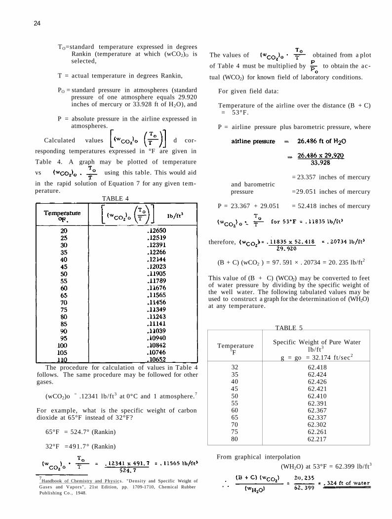
24

TO=standard temperature expressed in degrees Rankin (temperature at which (wCO2)O is selected,

T = actual temperature in degrees Rankin,

PO = standard pressure in atmospheres (standard pressure of one atmosphere equals 29.920 inches of mercury or 33.928 ft of H2O), and

P = absolute pressure in the airline expressed in atmospheres.

Calculated values o f a n d cor­responding temperatures expressed in °F are given in Table 4. A graph may be plotted of temperature vs using this table. This would aid

in the rapid solution of Equation 7 for any given tem­perature.

TABLE 4

The procedure for calculation of values in Table 4 follows. The same procedure may be followed for other gases.

(wCO2)o = .12341 lb/ft3 at 0°C and 1 atmosphere.7

For example, what is the specific weight of carbon dioxide at 65°F instead of 32°F?

65°F = 524.7° (Rankin)

32°F =491.7° (Rankin)

7Handbook of Chemistry and Physics . "Densi ty and Specific Weight of Gases and Vapors" , 21st Edition, pp. 1709-1710, Chemical Rubber Publishing Co., 1948.

The values of obtained from a plot

of Table 4 must be multiplied by to obtain the ac­

tual (WCO2) for known field of laboratory conditions.

For given field data:

Temperature of the airline over the distance (B + C) = 53°F.

P = airline pressure plus barometric pressure, where

= 23.357 inches of mercury and barometric pressure =29.051 inches of mercury

P = 23.367 + 29.051 = 52.418 inches of mercury

therefore,

(B + C) (wCO2 ) = 97. 591 × . 20734 = 20. 235 lb/ft2

This value of (B + C) (WCO2) may be converted to feet of water pressure by dividing by the specific weight of the well water. The following tabulated values may be used to construct a graph for the determination of (WH2O) at any temperature.

TABLE 5

Temperature OF

Specific Weight of Pure Water lb/ft3

g = go = 32.174 ft/sec2

32 62.418 35 62.424 40 62.426 45 62.421 50 62.410 55 62.391 60 62.367 65 62.337 70 62.302 75 62.261 80 62.217

From graphical interpolation (WH2O) at 53°F = 62.399 lb/ft3

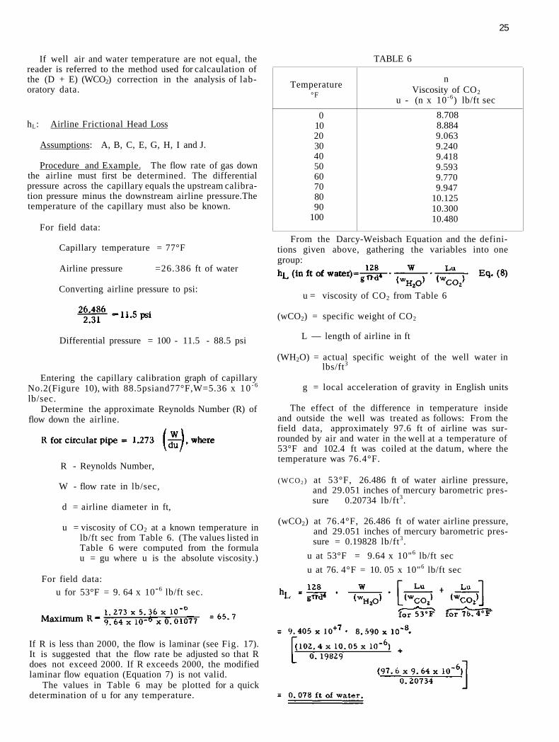
25

If well air and water temperature are not equal, the reader is referred to the method used for calcaulation of the (D + E) (WCO2) correction in the analysis of lab­oratory data.

hL: Airline Frictional Head Loss

Assumptions: A, B, C, E, G, H, I and J.

Procedure and Example. The flow rate of gas down the airline must first be determined. The differential pressure across the capillary equals the upstream calibra­tion pressure minus the downstream airline pressure.The temperature of the capillary must also be known.

For field data:

Capillary temperature = 77°F

Airline pressure =26.386 ft of water

Converting airline pressure to psi:

Differential pressure = 100 - 11.5 - 88.5 psi

Entering the capillary calibration graph of capillary No.2(Figure 10), with 88.5psiand77°F,W=5.36 x 10 - 6

lb/sec. Determine the approximate Reynolds Number (R) of

flow down the airline.

TABLE 6

Temperature °F

n Viscosity of CO2

u - (n x 10 -6) lb/ft sec 0

10 20 30 40 50 60 70 80 90

100

8.708 8.884 9.063 9.240 9.418 9.593 9.770 9.947

10.125 10.300 10.480

u = viscosity of CO2 from Table 6

(wCO2) = specific weight of CO2

L — length of airline in ft

(WH2O) = actual specific weight of the well water in lbs/ft3

g = local acceleration of gravity in English units

The effect of the difference in temperature inside and outside the well was treated as follows: From the field data, approximately 97.6 ft of airline was sur­rounded by air and water in the well at a temperature of 53°F and 102.4 ft was coiled at the datum, where the temperature was 76.4°F.

(WCO 2 ) at 53°F, 26.486 ft of water airline pressure, and 29.051 inches of mercury barometric pres­sure 0.20734 lb/ft3.

(wCO2) at 76.4°F, 26.486 ft of water airline pressure, and 29.051 inches of mercury barometric pres­sure = 0.19828 lb/ft3.

u at 53°F = 9.64 x 10"6 lb/ft sec u at 76. 4°F = 10. 05 x 10"6 lb/ft sec

R - Reynolds Number,

W - flow rate in lb/sec,

d = airline diameter in ft,

u = viscosity of CO2 at a known temperature in lb/ft sec from Table 6. (The values listed in Table 6 were computed from the formula u = gu where u is the absolute viscosity.)

For field data: u for 53°F = 9. 64 x 10-6 lb/ft sec.

If R is less than 2000, the flow is laminar (see Fig. 17). It is suggested that the flow rate be adjusted so that R does not exceed 2000. If R exceeds 2000, the modified laminar flow equation (Equation 7) is not valid.

The values in Table 6 may be plotted for a quick determination of u for any temperature.

From the Darcy-Weisbach Equation and the defini-tions given above, gathering the variables into one group:

26

B(wai r): Pressure Exerted by a Vertical Column of Air in the Casing Between the Datum and the Water Surface

Assumptions: B and J.

Procedure and Example: The B(wair) correction is the pressure difference in the air between the datum and the well water surface. The distance B is unknown, but it may be approximated by assuming that the pressure reading (Pr) is the true measure of the water level above the airline nozzle. This assumption is justified when calculating the B(wair) correction.

(w a i r) may be calculated from the following relation:8

(w a i r)= specific weight of air in the well in pounds per cubic foot.

Z = barometric pressure in inches of mer­cury

t = well air temperature in °F

X = moisture content of air in well (grains per pound of dry air)

For normal field ranges of barometric pressure, the moisture content of the air can be read directly from a psychrometric chart if the wet bulb temperature can be determined. The assumption was made that the air inside the well casing was saturated, thereby eliminating the need for measurement of the wet bulb temperature. For saturated air, the following values of X may be used to construct a graph of temperature vs moisture content of saturated air.

TABLE 7

X Well Temperature Grains of Moisture

°F per pound of dry air (Saturated air)

30 24 40 36 50 54 60 78 70 110 80 156 85 184

For field data, the approximate distance to water is

(B + C) - Pr or 97.591 - 26.486 = 71.105 ft.

B = 71.105 ft.

Well temperature - 53°F, X = 60, and Z = 29.051 inches of

mercury

Pb: Effective Bubble Pressure

The effective bubble pressure was evaluated by use of a graph plotted from laboratory test data shown in Figure 17. This graph is applicable only for the partic­ular nozzle shape described. Pb must lie somewhere be­tween 0.012 and 0.016 ft of water. The maximum bubble height curve was assumed to represent Pb.

The approximate pressure at bubble = P r .

For field data: Pressure at bubble =26.486 ft of H2O.

From Figure 17, Pb = 0.013 ft of H2O

Summary

All of the corrections in Equation (2) have now been evaluated, and converted to equivalent feet of water pressure. Pr is also expressed in feet of water. We may now apply Equation (2).

C(ft) = Pr + algebraic summation of corrections.

B(ft) - (B + C) - C.

For field data: C =26.486-0.078+0.324-0.084-0.013

=26.486+0.149 =26.635 ft

B=97.591-26.635 =70.956 ft

The corrected distance from the datum to the water sur­face inside the well is 70.956 ft.

Correction of Laboratory Data

The following will be limited to the analysis of a typical set of laboratory data. Th is will serve to dem­onstrate the procedures that were followed to secure results plotted on Figure 23.

(D + E) (wCO2): Pressure Exerted by a Vertical Column of CO2 in the Airline

Assumptions: D, E, G and J.

27

Example: Absolute pressure on CO2 in airline = (D + E) - D = barometric pressure:

= 16.261 + 28 .925 = 45.186 inches of m e r c u r y .

= 0. 106 ft of water

hL: Factional Head Loss

Assumptions: A, B, D, E, G, H and I. Example:

Capillary temperature - 7 9 . 4 ° F .

Airline pressure — 18.439 ft of water.

Capillary differential = upstream calibration pressure - 'downstream airline pressure.

From graph of calibration of Capillary No. 1,

W = 6 .03 x 10-6 l b / s e c .

(WCO2 ) for 55°F well water temp and air l ine p r e s s u r e = 0. 17807 lb/ft3 .

(wCO2 ) for 78 °F well a i r temp and a i r l ine p r e s s u r e = 0. 17040 lb/ft3 .

u for 55°F = 9. 68 x 1 0 - 6 lb/f t sec .

u for 78°F = 10. 08 x 1 0 - 6 lb / f t sec . E = 18. 44 ft, (50-E) = 31. 56 ft.

= 0. 025 ft of water

(D+F)(wCO 2 ) : Pressure Exerted by Vertical Column of CO 2 i n the Pressure Line.

Assumptions: B, F , G , J and K.

Example:

F = 20.197 - 1.720 = 18.477 ft.

D = 19.428 ft.

(D + F) =37.905 ft.

Pressure line temperature = 78°F.

= 16.294 +28.925 =45.219 inches of mercury.

Pb: Effective Bubble Pressure

Airline submergence — 18.439 ft of water — pressure at bubble.

From Figure 17, Pb = 0.014 ft of water

Summary

The computed corrections have been evaluated and con­verted to equivalent ft of water pressure.

(F - E) = 18.477 - 18.439 = 0.038 ft.

Computed corrections = 0.104 x 0.014 + 0.025-0.106 = 0.037 ft.

Error = 0.038 - 0.037= +0.001 ft.

28

APPENDIX II

OTHER SOURCES OF BUBBLER SYSTEM ERROR

This report deals in part with the development of the principle of bubbler system instrumentation and the cor­rection of data for "theoretical" errors. There are, how­ever, several other sources of error which affect the over-all accuracy of the system.

The most obvious source is error in the measurement of airline pressure at the datum. Manufacturers usually specify the accuracy of pressure-measuring devices as a percentage of the full-scale reading or by stating that any given reading is accurate to within one part in 100, 1000, 2000, etc. For example, if a recorder, accurate to one per cent (1 part in 100), were used to measure pressures in a 100-foot range, any given reading might be in error as much as one foot. It would be impossible to measure to 0.01 ft in a 100 ft range with a one per cent recorder. It is possible, however, to measure to 0.01 ft with a one per cent recorder in a one foot range. Laboratory tests indicate that the bubbler system, in­dependent of a pressure-indicating device, is accurate to within 0.014 ft for 95 per cent of the readings within any reasonable range. The choice of a suitable pressure recorder to go with this system is then a function of how much linear error is permissible. If the linear value of permissible error is several times larger than the sum­mation of the data corrections, these corrections may be disregarded. For example, it would be inconsistent to apply data corrections in the order of 0.2 ft to data that was only "good" to 0.5 ft originally.

The steel tape used to measure the distance from the datum to the bubbler nozzle is also a source of error. A 100-foot steel tape is 100 ft long only at a given temperature and tension. One hundred foot tapes that have been kinked or stretched or have been poorly manufactured are rarely 100.00 ft long at field tem­perature or tension. In order to determine the distance to the bubbler nozzle to within 0.01 ft, a tape must be used which has been recently checked against an ac­cepted standard under the same tension to be used in the field. The temperature must be known when the tape is being checked so that the field results can be "temperature corrected" for expansion or contraction. Information may be found in any book on surveying on procedures that are used for correcting steel tape mea­surements. Even when extreme precautions are taken, it is doubtful if measurements can be taken any closer than 0.005 ft in a 100-foot range.

In order to measure elevations with the bubbler sys­tem the specific gravity of the fluid must be known (see Figure 2). Note that in Table 5 the values of the specific weight are for pure water at a given tempera­ture and under the influence of the standard gravita­tional acceleration 32.174 ft/sec2 . Therefore, at least two other factors besides temperatures affect the specific weight of water as listed in Table 5: the total dissolved solids in the water and also the local acceleration of gravity.

Gravitational acceleration in Illinois ranges between 32.152 ft/sec2 (St. Louis) to 32.161 ft/sec2 (Chicago)

with 32.157 ft/sec2 at Urbana. The values of the specific weight of fresh water given in Table 5 should be mul­tiplied by g/go to obtain a specific weight of water which is corrected for gravitational effects. The total error caused by using values directly from Table 5 will be proportional to the submergence of the nozzle. For a 100-foot submergence the error could amount to 0.054 ft at Urbana. If a mercury manometer is used to measure airline pressure the gravitational effect need not be considered since the conversion factor from "feet of mercury" to "feet of water" is merely the ratio of the weight of a volume of mercury to the weight of an equal volume of water. Local variation in " g " from the standard value will also cause the values in Tables 4 and 6 to be slightly in error, but if these values are used in calculating the data corrections the linear error will be small since the corrections themselves are small in comparison to the water depth being measured.

Dissolved substances in the water, either mineral or gaseous, add to the specific weight. The amount of linear error when measuring water levels will be propor­tional to the submergence of the nozzle. If, for example, the fresh water in Table 5 contains 500 ppm total dis­solved minerals and 50 ppm dissolved gases, the linear error for a 100-foot submergence would be of the order of 0.05 ft. If extreme accuracy is required, the specific weight of the well water should be corrected from min­eral analysis data. An average over-all correction for the mineral content of the well water was determined to be 0.018 ft for the Gridley test. This additional cor­rection was not applied to the data reported in Figure 27 since it is only about 12 per cent of the summation of all the other corrections. There is considerable doubt whether this additional correction would be significant when compared to the float-operated recorder and the mercury manometer errors. If this correction had been. applied, the bubbler system and float recorder results would have been in even closer agreement.

In the laboratory test described previously, the data were not corrected for either gravitational effect or for dissolved minerals since the airline pressure was mea­sured in terms of the water being measured in the lab­oratory well.

If high velocities in the well were present moving either towards or away from the nozzle discharge area, an additional correction for a velocity head would be necessary. This error is caused by the Pitot effect. Velocities causing a measurable head are generally not present in an observation well and seldom in a pumped well unless the nozzle is located very near the pump intake. Reasonable effort should be made to locate the nozzle out of turbulent regions that usually occur at the pump intake.

In order to estimate the order of magnitude of errors caused by incorrect measurement (or complete disregard) of temperature it is necessary to break the discussion into parts. The specific weight of the well water is also a function of temperature. In Illinois, approximately

29

95 per cent of the wells tested have temperatures be­tween 50°F and 60°F. If an average value of 55°F were used throughout, a linear error of 0.028 ft would result with a 100-foot submergence and a 5°F error in temperature measurement. In general, every attempt should be made to measure well water temperature to the nearest degree if the nozzle submergence is between 50 and 100 ft and to the nearest two or three degrees if the nozzle submergence is less than 50 ft. If a mercury manometer is used to measure airline pressure the tem­perature of the air surrounding it must be known quite accurately (to the nearest degree). The specific weight of mercury is extremely sensitive to temperature. For example, a linear error of 0.049 ft would result with a 5° temperature error and a 100-foot submergence. In converting the mercury differential to "feet of water" it is imperative that the conversion factor be computed as the ratio of the actual specific weight of the mercury at its temperature to the actual specific weight of the water at its temperature.

Errors in temperature measurement also cause errors in the calculated values of the data corrections since viscosity and specific weight of the gas in the airline and also the capillary discharge are functions of tem­perature. It is difficult to make general statements

regarding the accuracy to which temperature measure­ments must be taken in this case. As a result of pre­liminary calculations made with the equipment used for the laboratory and field tests, an error of 5°F would not affect the accuracy of the calculated corrections significantly.

The calculated value of the hL, correction is subject to three sources of error other than gas density and vis­cosity: the weight discharge, the airline length, and the airline diameter. If the flow in the airline is laminar, the head loss value is directly proportional to the weight discharge and airline length and inversely proportional to the fourth power of the diameter. Therefore, per­centage errors in measurement of either the airline length or the flow rate will cause an identical percentage error in measurement of the head loss value. If a given percentage error is made in the measurement of the airline diameter the resultant percentage error in the head loss value may be as much as four times the original error. The amount of linear error resultant from a given percentage error will, of course, depend upon the magnitude of the head loss value. Therefore, if W (the flow rate) can be reduced to a small value, the linear effect of errors in measurement of temperature, specific weight, diameter and length will also be small and may be disregarded for simplicity.

30

APPENDIX III

LIST OF SYMBOLS

A,B,and C are distances measured in feet, A and (B + C) are known (used in conjunction with Figure 4 and the analysis of field data)

a = airline cross-sectional area, in ft2

C1 and C2 = constants in Equation (4)

D, E, and F are distances measured in ft where (D -+ E) is known (used in conjunction with Fig­ure 20 and the analysis of laboratory data)

d = airline diameter in ft

dh = total head loss over increment of airline length

dL = an increment of length measured down the airline

e = the base of natural logarithms, 2 . 7 1 8 . . . .

f = Darcy-Weisbach friction factor for incre­ment

g = local acceleration of gravity in English units

gO = standard acceleration of gravity 32.174 ft/sec2

S/gO = gravitational correction

h = manometer differential in ft of water evaluation of Pb test, page 28)

hL = frictional head loss in the airline ex­pressed in ft of water

L = length of airline in ft

P = absolute pressure in the airline expressed in atmospheres

Pa = atmospheric pressure

Pb = the effective pressure required to make a bubble form and break away at the nozzle elevation (expressed in ft of H2O)

PO = standard pressure in atmosphere (standard pressure of atmosphere equals 29.920 inches of mercury or 33.928 ft of H2O

Pr = pressure recorder reading in ft of water

pv = nRT: the ideal gas law, where p = absolute pressure, v = volume, T = absolute tem­perature, and nR is a constant depending upon the nature and weight density of the gas

P1 = pressure at top of airline, in lb/ft2

P2 = pressure at nozzle, in lb/ft2

R = Reynolds number

T = actual temperature in degrees Rankin

TO = standard temperature expressed in degrees Rankin (temperature at which (wCO2)O is selected).

t = well air temperature in °F

u = viscosity of CO2 at known temperature in lb/ft sec from Table 6. (The values listed in Table 6 were computed from the formu­la u = g p where p is the absolute vis­cosity)

u = absolute or dynamic viscosity of the purge gas at a known temperature.

V = velocity through increment or velocity of flow in ft/sec

W = flow rate of gas in lbs/sec

w1 = specific weight of the gas at the top of the airline in lb/ft3

(wa i r) = specific weight of air in lbs/ft3 at known atmospheric pressure and temperature con­ditions

(WCO 2 ) = specific weight of carbon dioxide gas un­der known temperature and pressure con­ditions expressed in lbs/ft3

(wCO2) = specific weight of CO2 under standard con­ditions of temperature, pressure, and gravi­tation in lbs/ft3

(wH2O) = actual specific weight of water at a known temperature in lbs/ft3

X = moisture content of air in well (grains per pound of dry air)

y = distance from bubbler nozzle to water sur­face (evaluation of Pb test, page 28)

Z = barometric pressure in inches of mercury

STATE OF ILLINOIS Department of Registration and Education

STATE WATER SURVEY DIVISION Urbana, Illinois

REPORTS OF INVESTIGATIONS

No. 1. Temperature and Turbidity of Some River Waters in Illinois. By Max Suter (1948).

No. 2. Groundwater Resources in Winnebago County, with Specific Reference to Conditions at Rockford. By H. F. Smith and T. E. Larson (1948).

No. 3. Radar and Rainfall. By G. E. Stout and F. A. Huff (1949). Out of print. No. 4. The Silt Problem of Spring Lake, Macomb, Illinois. By J. B. Stall, L. C.

Gottschalk, A. A. Klingebiel, E. L. Sauer, and E. E. DeTurk (1949). Out of print.

No. 5. Infiltration of Soils in the Peoria Area. By G. A. Stauffer (1949). No. 6. Groundwater Resources in Champaign County. By H. F. Smith (1950). No. 7. The Silting of Ridge Lake, Fox Ridge State Park, Charleston, Illinois. By

J. B. Stall, L. C. Gottschalk, A. A. Klingebiel, E. L. Sauer and S. W. Mel-sted (1951). Out of print.

No. 8. The Silting of Lake Chautauqua, Havana, Illinois, by J. B. Stall and S. W. Melsted (1951).

No. 9. The Silting of Carbondale Reservoir, Carbondale, Illinois. By B. O. Lar­son, A. A. Klingebiel, E. L. Sauer, S. W. Melsted, and R. C. Hay (1951). Out of print.

No. 10. The Silting of Lake Bracken, Galesburg, Illinois. By B. 0. Larson, A. A. Klingebiel, E. L. Sauer, and S. W. Melsted (1951).

No. 11. Irrigation in Illinois. By W. J. Roberts (1951). No. 12. The Silting of West Frankfort Reservoir, West Frankfort, Illinois. By J. B.

Stall, A. A. Klingebiel, S. W. Melsted and E. L. Sauer (1951). No. 13. Studies of Thunderstorm Rainfall with Dense Raingage Networks and

Radar (1951). Out of print. No. 14. The Storm of July 8, 1951 in North Central Illinois. (1952). No. 15. The Silting of Lake Calhoun, Galva, Illinois. By J. B. Stall, A. A. Klinge­

biel, S. A. Melsted and E. L. Sauer (1952). No. 16. The Silting of Lake Springfield, Springfield, Illinois. By J. B. Stall, L. C.

Gottschalk, and H. M. Smith (1952). No. 17. Preliminary Investigation of Groundwater Resources in the American Bot­

tom. By Jack Bruin and H. F. Smith (1953). No. 18. The Silting of Lake Carthage, Carthage, Illinois. By J. B. Stall, G. R. Hall,

S. W. Melsted, and E. L. Sauer (1953). No. 19. Rainfall-Radar Studies of 1951. By G. E. Stout, J. C. Neill, and G. W.

Farnsworth (1953). No. 20. Precipitation Measurements Study by John C. Kurtyka (1953). No. 21. Analysis of 1952 Radar and Raingage Data by J. C. Neill (1953). No. 22. Study of an Illinois Tornado Using Radar, Synoptic Weather and Field

Survey Data. By F. A. Huff, H. W. Hiser and S. G. Bigler (1954).