Btp Report

Game-theoretic analysis of 2-vendorbasic-commodity markets

May 13, 2009

B.Tech. Project Stage - II Report

Submitted in partial fulfillment of the requirements

for the degree of

Bachelor of Technology

by

Pushkar Agrawal

Roll No: 05005035

under the guidance of

Prof. Milind Sohoni

Department of Computer Science and Engineering

Indian Institute of Technology, Bombay

Mumbai

1

Acknowledgment

I am very thankful to my guide, Prof. Milind Sohoni, for his guidance and the motivation heprovided during the course of this project making this a great learning experience.

3

Contents

I Introduction 7

II Game Theory: Background 9

1 Strategic form games 10

1.1 Nash Equilibrium . . . . . . . . . . . . . . . . . . . . . . . . . . . . . . . . . . . . 11

III Problem Statement 15

2 Motivation: Economic relevance 15

3 Game-theoretic formulation 16

4 Overview of the analysis 17

IV Non-cooperative Analysis 19

5 Pure strategy equilibria 19

6 Randomized strategy equilibria 25

6.1 Payoff function and Bezier surfaces . . . . . . . . . . . . . . . . . . . . . . . . . . 27

6.2 Existence of mixed strategy equilibrium . . . . . . . . . . . . . . . . . . . . . . . 29

6.3 A trivial mixed strategy equilibrium . . . . . . . . . . . . . . . . . . . . . . . . . 35

6.4 Mixed strategy segmentation in the market . . . . . . . . . . . . . . . . . . . . . 36

6.4.1 Condition 1 . . . . . . . . . . . . . . . . . . . . . . . . . . . . . . . . . . . 36

6.4.2 Condition 2 . . . . . . . . . . . . . . . . . . . . . . . . . . . . . . . . . . . 49

6.5 Prices in segmentation . . . . . . . . . . . . . . . . . . . . . . . . . . . . . . . . . 54

V Conclusion and Future Work 64

VI References 65

5

Part I

IntroductionSince times immemorial there have been economic disparities in the societies which lead tounequal purchasing powers of the fortunate and the less fortunate ones. However, both classesof the society consume certain basic commodities like milk, rice, loom etc. which do not haveany intrinsic monetary price of their own at which their trade should occur. The selling priceof such commodities are decided by the demand of the buyers, the price they are willing to payand the profit-maximizing motives of the seller.

Thus, in a society where there is a fixed price for the basic commodities, there will always be asection of the society to which this price will not be affordable and will be consequently affectedeven though there may be an excess supply of the commodity which could have been sold tothe less formulate ones but was not because of the decided selling price. Thus, advocating thecontinuance of more than one marketplace for such commodities becomes important so thatall economic sections of the society can afford to get hold of the basic commodities. As theNobel Prize winning economist Amartya Sen has argued, the reason for most of the faminesdid not lie in the shortage of food but in its distribution system, a study of the effect of morethan one marketplaces for the same commodity in an economically disparate society may giveus insights into the strategic behavior (of the buyers) to be considered while designing bettermarket mechanisms.

In this report, we shall analyze the decision making situation faced by the unequal sections ofthe society when they have the option of going to two identical vendors.

7

Part II

Game Theory: BackgroundGame theory is the study of strategic interactions between rational and intelligent decisionmakers or players capable of performing actions that affect everyone’s welfare.

Game theoretic analysis involves conceiving a problem as a situation or a game in which thereare two or more individuals or players. Each individual is capable of performing some actions.The benefit or the payoff received by any player is a function of the actions of all. As an example,consider a situation in which you and your friend want to buy a painting for themselves at ashop. The shopkeeper sells the painting to one who offers the most. In this game, you andyour friend are the players and your actions are the different bids you would place. The resultof your bids (actions) depends on your friend’s bids (actions) also.

Game theoretic analysis assumes that the players be rational and intelligent. What do wemean by “rationality” ? Nobel laureate Robert J. Aumann [3], in his prize lecture defines it as:

"A person’s behavior is rational if it is in his best interest, given his informa-tion"

Mathematically, one can say that a rational player should act in a way so as to maximize hisexpected payoff being measured on some utility scale. A utility scale can be thought of as aquantitative characterization of a players’ preferences for the outcomes of the game. That is,an outcome with utility 1 is preferable over an outcome with utility 0.5 . It must be noted thatthese utility numbers do not carry any meaning in them. They only indicate the preferences ofthe players over the outcomes. As long as the preferences are properly depicted, these valuescan be anything. John von Neumann and Oskar Morganstern proved the theorem - that for anyrational decision maker there exists some way of assigning utility numbers to various possibleoutcomes that he cares about such that he would always choose the option that maximizes hisexpected utility - called the expected utility maximization theorem. So, mathematically, rationalbehavior means maximizing expected utility.

What do we mean by “intelligence” ? A player is said to be intelligent if he knows abouteverything about the game what a game-theoretic analyst knows about the game, he can analyzeand conclude what ever any great game theorist can analyze about the game. The assumptionof intelligent player requires that the players should be able to anticipate the implications drawnfrom the game theoretic analysis of the game they are in.

We shall now study about modeling a conflict situation as a game.

9

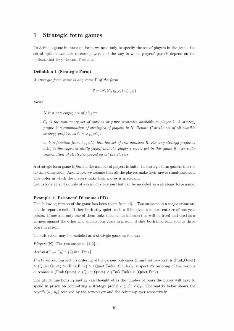
1 Strategic form games

To define a game in strategic form, we need only to specify the set of players in the game, theset of options available to each player, and the way in which players’ payoffs depend on theoptions that they choose. Formally,

Definition 1 (Strategic Form)

A strategic form game is any game Γ of the form

Γ = (N, (Ci)i∈N , (ui)i∈N )

where

- N is a non-empty set of players.

- Ci is the non-empty set of options or pure strategies available to player i. A strategyprofile is a combination of strategies of players in N. Denote C as the set of all possiblestrategy profiles, so C = ×j∈NCj.

- ui is a function from ×j∈NCj into the set of real numbers R. For any strategy profile c,ui(c) is the expected utility payoff that the player i would get in this game if c were thecombination of strategies played by all the players.

A strategic form game is finite if the number of players is finite. In strategic form games, there isno time dimension. And hence, we assume that all the players make their moves simultaneously.The order in which the players make their moves is irrelevant.Let us look at an example of a conflict situation that can be modeled as a strategic form game.

Example 1: Prisoners’ Dilemma (PD)The following version of the game has been taken from [4]. Two suspects in a major crime areheld in separate cells. If they both stay quiet, each will be given a minor sentence of one yearprison. If one and only one of them finks (acts as an informer) he will be freed and used as awitness against the other who spends four years in prison. If they both fink, each spends threeyears in prison.

This situation may be modeled as a strategic game as follows:

Players(N): The two suspects {1,2}.

Actions(C1= C2) : {Quiet, Fink}.

Preferences: Suspect 1’s ordering of the various outcomes (from best to worst) is (Fink,Quiet)> (Quiet,Quiet) > (Fink,Fink) > (Quiet,Fink). Similarly, suspect 2’s ordering of the variousoutcomes is (Fink,Quiet) < (Quiet,Quiet) < (Fink,Fink) < (Quiet,Fink).

The utility functions u1 and u2 can thought of as the number of years the player will have tospend in prison on committing a strategy profile c ∈ C1 × C2. The matrix below shows thepayoffs (u1, u2) received by the row-player and the column-player respectively.

10

Suspect 2

Quiet FinkSuspect 1 Quiet 2,2 0,3

Fink 3,0 1,1

The Prisoner’s Dilemma models a situation in which there are gains from cooperation but eachplayer has an incentive to free ride whatever the other player does.

Example 2: Bach or Stravinsky (BOS)The following version of the game has been taken from [4]. Two people wish to go out together(call them husband and wife). Two concerts are available: one of music by Bach and other byStravinsky. One person prefers Bach and the other person prefers Stravinsky. If they go todifferent concerts, each of them is equally unhappy listening to the music of either composer.

This situation may be modeled as a strategic game as follows:

Players(N): The two suspects {Husband, Wife}.

Actions(C1= C2) : {Bach, Stravinsky}.

Preferences: Husband’s ordering of the various outcomes (assuming he prefers Bach) is (Bach,Bach) > (Stravinsky,Stravinsky) > (Bach, Stravinsky) = (Stravinsky, Bach). Similarly, sus-pect 2’s ordering of the various outcomes is (Stravinsky,Stravinsky) > (Bach, Bach) > (Bach,Stravinsky) = (Stravinsky, Bach).

The matrix below shows the payoffs (u1, u2) received by the row-player and the column-playerrespectively.

Wife

Bach StravinskyHusband Bach 2,1 0,0

Stravinsky 0,0 1,2

1.1 Nash Equilibrium

Given a game in strategic form, we are interested in finding out what would rational playersdo in the scenario presented by the game. A player’s best action (or strategy) depends on theother players’ actions also. So, when choosing an action, a player must also take into accountthe actions that would be chosen by his opponents. That is, he should form beliefs about theother players’ actions. A solution concept that incorporates the two facts - (i) the players arerational (expected utility maximizers) and (ii) the beliefs of one player about the actions ofother players are correct in the sense that beliefs of two players about actions of a third playerare the same - is that of Nash Equilibrium.

Informally, a Nash equilibrium of a game is a strategy profile s such that no player i can bebetter off by deviating from the strategy si listed for him in s given that the other players j(j 6= i) adhere to their strategies sj as listed in s.

Before defining Nash equilibrium of a strategic form game, we shall study some terminology. Wehave already seen what do we mean by pure strategy so, let us define randomized strategy

11

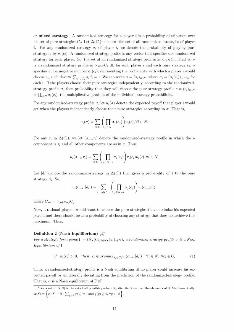
or mixed strategy. A randomized strategy for a player i is a probability distribution overhis set of pure strategies Ci. Let ∆(Ci)1 denotes the set of all randomized strategies of playeri. For any randomized strategy σi of player i, we denote the probability of playing purestrategy ci by σi(ci). A randomized strategy profile is any vector that specifies one randomizedstrategy for each player. So, the set of all randomized strategy profiles is ×i∈NCi. That is, σis a randomized strategy profile in ×i∈NCi iff, for each player i and each pure strategy ci, σspecifies a non negative number σi(ci), representing the probability with which a player i wouldchoose ci, such that ∀i

∑di∈Ci σidi = 1.We can write σ = (σi)i∈N , where σi = (σi(ci))ci∈Ci for

each i. If the players choose their pure strategies independently, according to the randomized-strategy profile σ, then probability that they will choose the pure-strategy profile c = (ci)i∈Nis∏i∈N σi(ci), the multiplicative product of the individual strategy probabilities.

For any randomized-strategy profile σ, let ui(σ) denote the expected payoff that player i wouldget when the players independently choose their pure strategies according to σ. That is,

ui(σ) =∑c∈C

( ∏j∈N

σj(cj)

)ui(c),∀i ∈ N.

For any τi in ∆(Ci), we let (σ−i,τi) denote the randomized-strategy profile in which the i-component is τi and all other components are as in σ. Thus,

ui(σ−i, τi) =∑c∈C

( ∏j∈N−i

σj(cj)

)τi(ci)ui(c),∀i ∈ N.

Let [di] denote the randomized-strategy in ∆(Ci) that gives a probability of 1 to the purestrategy di. So,

ui(σ−i, [di]) =∑

c−i∈C−i

( ∏j∈N−i

σj(cj)

)ui(c−i, di).

where C−i = ×j∈N−jCj .

Now, a rational player i would want to choose the pure strategies that maximize his expectedpayoff, and there should be zero probability of choosing any strategy that does not achieve thismaximum. Thus,

Definition 2 (Nash Equillibrium) [3]For a strategic form game Γ = (N, (Ci)i∈N , (ui)i∈N ), a randomized-strategy profile σ is a NashEquillibrium of Γ

if σi(ci) > 0, then ci ∈ argmaxdi∈Ciui(σ−i, [di]) ∀i ∈ N, ∀ci ∈ Ci (1)

Thus, a randomized-strategy profile is a Nash equilibrium iff no player could increase his ex-pected payoff by unilaterally deviating from the prediction of the randomized-strategy profile.That is, σ is a Nash equilibrium of Γ iff

1For a set S, ∆(S) is the set of all possible probability distributions over the elements of S. Mathematically,

∆(S) ={q : S → R |

∑y∈S q (y) = 1 and q (y) ≥ 0, ∀y ∈ S

}.

12

ui(σ) ≥ ui(σ−i, τi), ∀i ∈ N, ∀τi ∈ ∆(Ci). (2)

An equilibrium strategy profile that consists of pure strategies only is called an equilibrium inpure strategies.

We will now see a theorem that guarantees existence of Nash equilibrium.

Theorem 3 (Existence of Nash Equillibrium) [3]For a finite game Γ = (N, (Ci)i∈N , (ui)i∈N ) in strategic form, there exists at least one equillib-rium in ×i∈N∆(Ci).

Randomized strategies are required to prove this existence theorem because many games haveno equilibria in pure strategies.

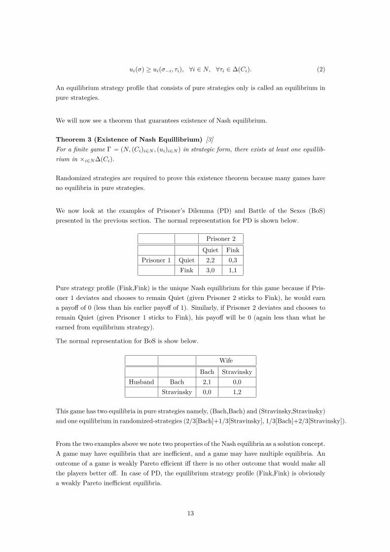
We now look at the examples of Prisoner’s Dilemma (PD) and Battle of the Sexes (BoS)presented in the previous section. The normal representation for PD is shown below.

Prisoner 2

Quiet FinkPrisoner 1 Quiet 2,2 0,3

Fink 3,0 1,1

Pure strategy profile (Fink,Fink) is the unique Nash equilibrium for this game because if Pris-oner 1 deviates and chooses to remain Quiet (given Prisoner 2 sticks to Fink), he would earna payoff of 0 (less than his earlier payoff of 1). Similarly, if Prisoner 2 deviates and chooses toremain Quiet (given Prisoner 1 sticks to Fink), his payoff will be 0 (again less than what heearned from equilibrium strategy).

The normal representation for BoS is show below.

Wife

Bach StravinskyHusband Bach 2,1 0,0

Stravinsky 0,0 1,2

This game has two equilibria in pure strategies namely, (Bach,Bach) and (Stravinsky,Stravinsky)and one equilibrium in randomized-strategies (2/3[Bach]+1/3[Stravinsky], 1/3[Bach]+2/3[Stravinsky]).

From the two examples above we note two properties of the Nash equilibria as a solution concept.A game may have equilibria that are inefficient, and a game may have multiple equilibria. Anoutcome of a game is weakly Pareto efficient iff there is no other outcome that would make allthe players better off. In case of PD, the equilibrium strategy profile (Fink,Fink) is obviouslya weakly Pareto inefficient equilibria.

13

Part III

Problem Statement

2 Motivation: Economic relevance

Consider an example of a milk vendor.

Ramesh owns a cow which gives 10 litre of milk every morning. Each night, village men cometo Ramesh and submit their bids, each of which consists of the amount of milk wanted the nextmorning and the price he is willing to pay. Ramesh looks at the bids and comes up with a pricewhich maximizes the profit he can earn by selling some or all of the milk. Let the following bethe list of the villagers with their bids (arranged in increasing order of their affordable price)that arrive on a typical night at Ramesh’s.

Villager Quantity-Demanded (q) Price affordable (p) Profit to Ramesh by selling at price p

M112 Rs. 2 Rs. 13

M2 1 Rs. 2 Rs. 12M3 1 Rs. 3 Rs. 25M4

12 Rs. 4 Rs. 24

M5 1 Rs. 9 Rs. 31 12

M6 1 12 Rs. 11 Rs. 27 1

2M7

12 Rs. 12 Rs. 12

M812 Rs. 14 Rs. 7

The price announced by Ramesh will be Rs. 9 as it gives the maximum profit = Rs. 3112 . All

the villagers bidding a price ≥ Rs. 9 will get the amount of milk they requested. M1 to M4

get nothing. The total milk sold is equal to (that purchased by M5 to M8) is 3 12 litre and the

rest 6 12 litre is wasted. This implies that even though there is an amount of commodity left

unsold and going wasted, there is a section of people who a deprived of its purchase due to themarket/distribution mechanism employed.

If there were an identical vendor in the village, say Ramesh’s cousin - Dinesh, then the villagerswho were denied of purchase at Ramesh’s can get the milk at Dinesh’s.. The price here wouldbe Rs. 2 (considering only M1 to M4) - making all the remaining villagers eligible for purchase.

So, what we see in the above example is that that the presence of two identical vendors madeall the villagers able to make a purchase despite the differences in their affordability.

But this is jut one realization of the buyers’ behavior out of the many possible ones and toadvocate the establishment of a second vendor requires guarantees that this buyer behavioris the most likely one and the one which is the best for each buyer. Establishment of suchguarantees requires that we somehow prove this behavior to be an equilibrium of this milkmarket with two vendors.

15

This report endeavors to establish such guarantees by performing a game-theoretic analysis ofthis situation and proves that the buyer behavior, pointed out above, is a Nash equilibrium -the natural order - of the situation.

Hence, we begin our analysis in earnest.

3 Game-theoretic formulation

Consider a scenario in which there are two types of buyers, rich (R) and poor (P) who want topurchase one unit of the same commodity (say, milk). There are two vendors V1 and V2 withquantities Q1 and Q2 of that commodity. The rich type of buyer bids a price of pR (in lightof the above example, pR can be seen to be the minimum price a rich can stoop to pay) and apoor type of buyer bids a price of pP (< pR) (again, in light of the above example, pP can beseen to be the maximum price a poor can dare to pay). The buyers submit their bids (or theprice they can afford to pay for that commodity) to either of the two vendors and wait for theselling price to be announced. Both the vendors look at the bids received and announce a pricethat maximizes their individual profit (= quantity_sold × selling_price). The vendors do notvalue their commodities at all, that is, there is no manufacturing cost involved. All the buyerswho can afford the price announced by their chosen vendor get a payoff which is equal to thefraction of their demand met, otherwise they get a nil payoff. If quantity available to sell is lessthan the demand faced, equal fractions of the quantity are distributed among all the eligiblebuyers.We now formally model the game in strategic form. Let Γ =

(N ∪M, (Ci)i∈N∪M , (ui)i∈N∪M

)be the strategic form game where:

• N is the set of poor buyers. |N | = n,

• M is the set of rich buyers. |M | = m,

• The set of moves for every buyer is Ci = {0, 1}∀i ∈ N ∪M , where move 0 correspondsto choosing to go to V1 and move 1 corresponds to choosing to go to V2. Apart from thechoice between the two vendors, the rich type of buyer (viz. i ∈ M) bids a price of pRand a poor type of buyer (viz. j ∈ N) bids a price of pP (< pR). Also, both types of thebuyers demand one unit of the commodity.

• The utility function ui : {0, 1}n+m → [0, 1] is the fraction of commodity obtained bybuyer i.

Let p (0 ≤ p ≤ n) poor and r (0 ≤ r ≤ m) rich buyers go to vendor Vk (kε {1, 2}) and let xk(p, r)and yk(p, r) be the payoffs earned by poor and rich buyers respectively, after Vk announces hisselling price. Then, the profit made by Vk by selling at pP (the price affordable to poor) ismin {Qk, p+ r} × pP . And the profit made by Vk by selling at pR ( price not affordable topoor) is min {Qk, r} × pR. Thus, for min {Qk, p+ r} × pP ≥min {Qk, r} × pR, poor and richearn the same non zero payoff equal to the fraction min{Qk,p+r}

p+r , otherwise, poor earn a payoffof zero and rich earn a payoff of min{Qk,r}

r . Let Xk and Yk be the pure strategy payoff matriceswith the (i, j)− th entry corresponding to the payoff earned by poor and rich respectively when

16

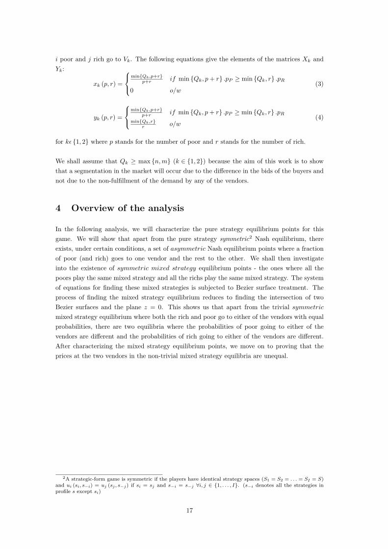
i poor and j rich go to Vk. The following equations give the elements of the matrices Xk andYk:

xk (p, r) =

min{Qk,p+r}

p+r if min {Qk, p+ r} .pP ≥ min {Qk, r} .pR0 o/w

(3)

yk (p, r) =

min{Qk,p+r}

p+r if min {Qk, p+ r} .pP ≥ min {Qk, r} .pRmin{Qk,r}

r o/w(4)

for kε {1, 2} where p stands for the number of poor and r stands for the number of rich.

We shall assume that Qk ≥ max {n,m} (k ∈ {1, 2}) because the aim of this work is to showthat a segmentation in the market will occur due to the difference in the bids of the buyers andnot due to the non-fulfillment of the demand by any of the vendors.

4 Overview of the analysis

In the following analysis, we will characterize the pure strategy equilibrium points for thisgame. We will show that apart from the pure strategy symmetric2 Nash equilibrium, thereexists, under certain conditions, a set of asymmetric Nash equilibrium points where a fractionof poor (and rich) goes to one vendor and the rest to the other. We shall then investigateinto the existence of symmetric mixed strategy equilibrium points - the ones where all thepoors play the same mixed strategy and all the richs play the same mixed strategy. The systemof equations for finding these mixed strategies is subjected to Bezier surface treatment. Theprocess of finding the mixed strategy equilibrium reduces to finding the intersection of twoBezier surfaces and the plane z = 0. This shows us that apart from the trivial symmetricmixed strategy equilibrium where both the rich and poor go to either of the vendors with equalprobabilities, there are two equilibria where the probabilities of poor going to either of thevendors are different and the probabilities of rich going to either of the vendors are different.After characterizing the mixed strategy equilibrium points, we move on to proving that theprices at the two vendors in the non-trivial mixed strategy equilibria are unequal.

2A strategic-form game is symmetric if the players have identical strategy spaces (S1 = S2 = . . . = SI = S)and ui (si, s−i) = uj (sj , s−j) if si = sj and s−i = s−j ∀i, j ∈ {1, . . . , I}. (s−i denotes all the strategies inprofile s except si)

17

Part IV

Non-cooperative Analysis

5 Pure strategy equilibria

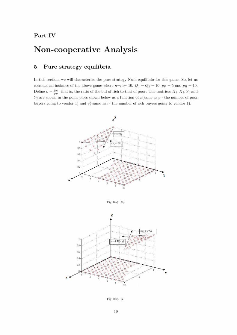
In this section, we will characterize the pure strategy Nash equilibria for this game. So, let usconsider an instance of the above game where n=m= 10. Q1 = Q2 = 10, pP = 5 and pR = 10.Define k = pR

pP, that is, the ratio of the bid of rich to that of poor. The matrices X1, X2, Y1 and

Y2 are shown in the point plots shown below as a function of x(same as p - the number of poorbuyers going to vendor 1) and y( same as r- the number of rich buyers going to vendor 1).

Fig 1(a). X1

Fig 1(b). X2

19

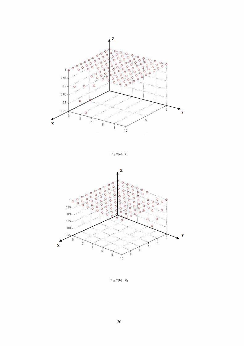
Fig 2(a). Y1

Fig 2(b). Y2

20

Two trivial Nash equilibria exist for the game. Firstly, the one in which all the poor go toV1and all the rich go to V2 and secondly, the one in which all the poor go to V2 and all the richgo to V1.

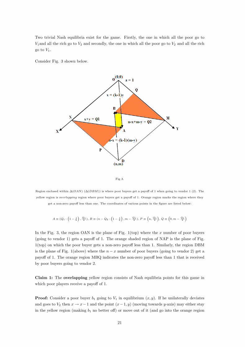
Consider Fig. 3 shown below.

Fig 3.

Region enclosed within ∆(OAN) (∆(DBM)) is where poor buyers get a payoff of 1 when going to vendor 1 (2). The

yellow region is overlapping region where poor buyers get a payoff of 1. Orange region marks the region where they

get a non-zero payoff less than one. The coordinates of various points in the figure are listed below:

A ≡ (Q1 ·(1− 1

k

),Q1k ), B ≡ (n−Q2 ·

(1− 1

k

),m− Q1

k ), P ≡(n,

Q1k

), Q ≡

(0,m− Q1

k

)In the Fig. 3, the region OAN is the plane of Fig. 1(top) where the x number of poor buyers(going to vendor 1) gets a payoff of 1. The orange shaded region of NAP is the plane of Fig.1(top) on which the poor buyer gets a non-zero payoff less than 1. Similarly, the region DBMis the plane of Fig. 1(above) where the n− x number of poor buyers (going to vendor 2) get apayoff of 1. The orange region MBQ indicates the non-zero payoff less than 1 that is receivedby poor buyers going to vendor 2.

Claim 1: The overlapping yellow region consists of Nash equilibria points for this game inwhich poor players receive a payoff of 1.

Proof: Consider a poor buyer b1 going to V1 in equilibrium (x, y). If he unilaterally deviatesand goes to V2 then x→ x−1 and the point (x−1, y) (moving towards y-axis) may either stayin the yellow region (making b1 no better off) or move out of it (and go into the orange region

21

making b1 worse off). Similarly, if any buyer b2 going to V2 unilaterally deviates and goes to V1,then x→ x+ 1 and the point (x+ 1, y) is either in the yellow region (making b2 no better off)or go into the orange region (making b2 worse off). Hence, points in the yellow (overlapping)region are Nash equilibrium points for this game.

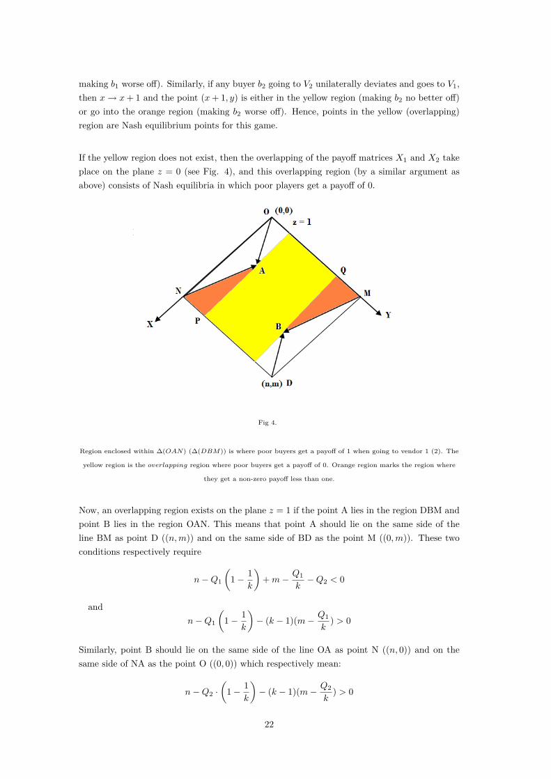
If the yellow region does not exist, then the overlapping of the payoff matrices X1 and X2 takeplace on the plane z = 0 (see Fig. 4), and this overlapping region (by a similar argument asabove) consists of Nash equilibria in which poor players get a payoff of 0.

Fig 4.

Region enclosed within ∆(OAN) (∆(DBM)) is where poor buyers get a payoff of 1 when going to vendor 1 (2). The

yellow region is the overlapping region where poor buyers get a payoff of 0. Orange region marks the region where

they get a non-zero payoff less than one.

Now, an overlapping region exists on the plane z = 1 if the point A lies in the region DBM andpoint B lies in the region OAN. This means that point A should lie on the same side of theline BM as point D ((n,m)) and on the same side of BD as the point M ((0,m)). These twoconditions respectively require

n−Q1

(1− 1

k

)+m− Q1

k−Q2 < 0

andn−Q1

(1− 1

k

)− (k − 1)(m− Q1

k) > 0

Similarly, point B should lie on the same side of the line OA as point N ((n, 0)) and on thesame side of NA as the point O ((0, 0)) which respectively mean:

n−Q2 ·(

1− 1k

)− (k − 1)(m− Q2

k) > 0

22

andn−Q2

(1− 1

k

)+m− Q2

k−Q1 < 0

These give us the conditions:k ≤ m+ n

m(5)

m+ n ≤ Q1 +Q2 (6)

So, the Nash equilibria of the above game are listed as follows:-

1. All poor buyers going to V1 and all rich buyers going to V2,

2. All poor buyers going to V2 and all rich buyers going to V1,

3. If the parameters of the game (viz. m,n, k,Q1, Q2) satisfy equations (3) and (4), thenall the points

(x, y) ε {(x, y) | x ≥ (k − 1)y, x+ y ≤ Q1, n− x ≥ (k − 1)(m− y) and n− x+m− y ≤ Q2 }

else all the points

(x, y)ε{

(x, y) | Q1k≤ y ≤ m− Q2

k

}.

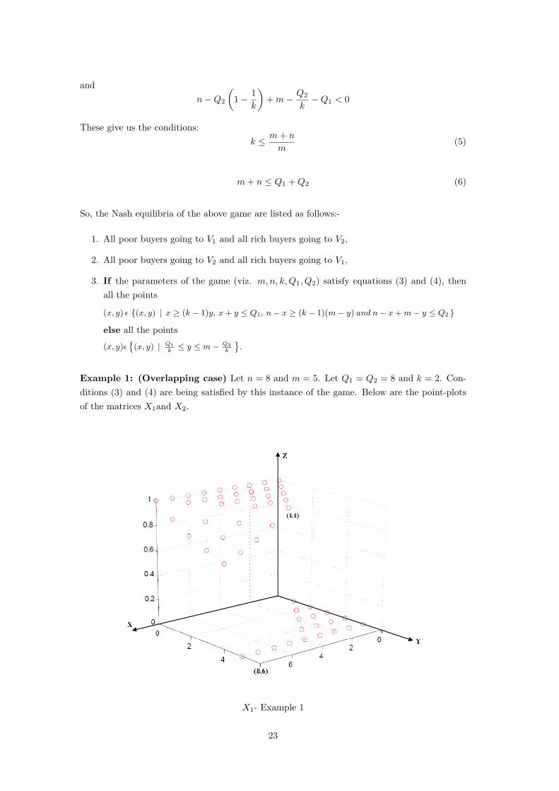
Example 1: (Overlapping case) Let n = 8 and m = 5. Let Q1 = Q2 = 8 and k = 2. Con-ditions (3) and (4) are being satisfied by this instance of the game. Below are the point-plotsof the matrices X1and X2.

X1- Example 1

23

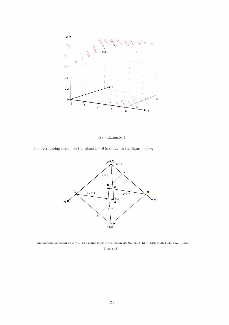
X2 - Example 1

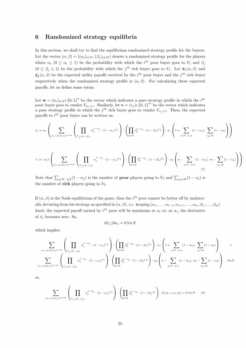
The overlapping region on the plane z = 0 is shown in the figure below:

The overlapping region on z = 0. The points lying in the region ACBD are {(4,1), (4,2), (4,3), (4,4), (5,2) (5,3),

(3,2), (3,3)}

24

6 Randomized strategy equilibria

In this section, we shall try to find the equilibrium randomized strategy profile for the buyers.Let the vector (α, β) = ((αi)i∈N , (βj)j∈M ) denote a randomized strategy profile for the playerswhere αi (0 ≤ αi ≤ 1) be the probability with which the ith poor buyer goes to V1 and βj

(0 ≤ βj ≤ 1) be the probability with which the jth rich buyer goes to V1. Let xi (α, β) andyj (α, β) be the expected utility payoffs received by the ith poor buyer and the jth rich buyerrespectively when the randomized strategy profile is (α, β). For calculating these expectedpayoffs, let us define some terms.

Let w = (wi)iεN ε {0, 1}n be the vector which indicates a pure strategy profile in which the ithpoor buyer goes to vendor Vwi+1. Similarly, let v = (vj)ε {0, 1}m be the vector which indicatesa pure strategy profile in which the jth rich buyer goes to vendor Vvj+1. Then, the expectedpayoffs to ith poor buyer can be written as:

xi = αi·

∑(w,v)ε{0,1}n+m

∏wjεN−{i}

α1−wjj

· (1− αj)wj

·(∏kεM

β1−vkk

· (1− βk)vk

)· x1

1 +∑

jεN−{i}

(1− wj),∑vkεM

(1− vk)

+ (1−αi)·

∑(w,v)ε{0,1}n+m

∏wjεN−{i}

α1−wjj

· (1− αj)wj

·(∏kεM

β1−vkk

· (1− βk)vk

)· x2

n−∑

jεN−{i}

(1− wj), m−∑vkεM

(1− vk)

(7)

Note that∑jεN−{i}(1− wj) is the number of poor players going to V1 and

∑vkεM

(1− vk) isthe number of rich players going to V1.

If (α, β) is the Nash equilibrium of the game, then the ith poor cannot be better off by unilater-ally deviating from his strategy as specified in (α, β), i.e. keeping (α1, . . . , αi−1, αi+1, . . . , αn, β1, . . . , βm)fixed, the expected payoff earned by ith poor will be maximum at αi or, at αi, the derivativeof xi becomes zero. So,

∂xi/∂αi = 0∀iεN

which implies:

∑(w,v)ε{0,1}n+m

∏wjεN−{i}

α1−wjj

· (1− αj)wj

·(∏kεM

β1−vkk

· (1− βk)vk

)· x1

1 +∑

jεN−{i}

(1− wj),∑vkεM

(1− vk)

=

∑(w,v)ε{0,1}n+m

∏wjεN−{i}

α1−wjj

· (1− αj)wj

·(∏kεM

β1−vkk

· (1− βk)vk

)· x2

n−∑

jεN−{i}


(1− vk)

∀iεN

or,

∑(w,v)ε{0,1}n+m

∏wjεN−{i}

α1−wjj

· (1− αj)wj

·(∏kεM

β1−vkk

· (1− βk)vk

)· Ti(w, v, n,m) = 0 ∀iεN (9)

25

where

Ti(w, v, n,m) = x1

1 +∑

jεN−{i}

(1− wj),∑vkεM

(1− vk)

− x2

n−∑

jεN−{i}


(1− vk)

Similarly, writing the expected payoff for the jth rich buyer and performing the above similaranalysis, we will get:

∑(w,v)ε{0,1}n+m

∏wjεN

α1−wjj

· (1− αj)wj

·( ∏kεM−{i}

β1−vkk

· (1− βk)vk

)· Si(w, v, n,m) = 0 ∀iεM (10)

where

Si(w, v, n,m) = y1

∑jεN

(1− wj), 1 +∑

vkεM−{i}

(1− vk)

− y2

n−∑jεN

(1− wj), m−∑

vkεM−{i}

(1− vk)

We shall analyze the existence of symmetric equilibria in a sense that all the poor play the samestrategy in equilibrium and all the rich play the same strategy in equilibrium. For this, we letall the αi’s to be equal to, say, α and all the βj ’s to be equal to, say, β. As a result, one canwrite the equations (9) and (10) as:

n−1∑p=0

m∑r=0

(n− 1p

)· αp · (1− α)n−p−1 ·

(mr

)· βr · (1− β)m−r · (x1 (p+ 1, r)− x2 (n− p,m− r)) = 0 (11)

and

n∑p=0

m−1∑r=0

(np

)· αp · (1− α)n−p ·

(m− 1r

)· βr · (1− β)m−r−1 · (y1 (p, r − 1)− y2 (n− p,m− r)) = 0 (12)

respectively.

In the above equations, α and β are scalars.

Note that there is a reason as to why we wrote the payoff function of the buyers as a functionof there mixed strategy profile where all αi’s and βj ’s were unequal because differentiating thepayoff function which is a function of α (α being the equal probability of all poor choosing V1

in equilibrium) would mean that we are checking whether the deviation of whole of the team ofpoor from the current equilibrium point lead to any better payoff for all - which is essentiallyanalyzing the grand coalition of all the poor and which is not what we intend to do. Since wewish to find the equilibrium mixed strategy which is individually best for all the poor (and forthe rich) and which is symmetric3 for poor and for rich, we take the above approach.

3a symmetric equilibrium is an equilibrium where both players use the same strategy (possibly mixed) in theequilibrium.

26

6.1 Payoff function and Bezier surfaces

Let us now look at how the equations (11) and (12) can be solved for α and β.

Identifying the expression(mr

)·βr · (1− β)m−r as the Bernstein polynomial Bmr (β), one can

re-write the equations (11) and (12) as:

n−1∑p=0

m∑r=0

Bn−1p (α) ·Bmr (β) · (x1 (p+ 1, r)− x2 (n− p,m− r)) = 0 (13)

n∑p=0

m−1∑r=0

Bnp (α) ·Bm−1r (β) · (y1 (p, r + 1)− y2 (n− p,m− r)) = 0 (14)

respectively. The solution (α, β) to the above two equations will give us a Nash equilibrium inrandomized strategies.

The above two equations have a very well known form, namely the Bezier surface, whichhas been extensively studied in the curve approximation literature of mathematics. A tensorproduct bezier surface of degrees (m,n) given by (m+ 1)× (n+ 1) matrix P of control pointsis defined as f : I2 → R3 (where I ≡ [0, 1]) such that:

f(u, v) =m∑i=0

n∑j=0

P [i, j] ·Bmi (u) ·Bmj (v)

We shall now define some terms to fit the Equations (13) and (14) into the framework of beziersurfaces.

Let gn−1,m : [0, 1]2 → R and hn,m−1 : [0, 1]2 → R be two functions and let Gn−1,m :{0, . . . , n− 1} × {0, . . . ,m} → [0, 1] and Hn,m−1 : {0, . . . , n} × {0, . . . ,m− 1} → [0, 1] betwo matrices with entries defined as:

Gn−1,m[i, j] = gn−1,m( i

n− 1,j

m) = x1 (i+ 1, j)− x2 (n− i,m− j) (15)

andHn,m−1[i, j] = hn,m−1(

i

n,

j

m− 1) = y1 (i, j + 1)− y2 (n− i,m− j) (16)

then, the equations (13) and (14) can be written as:

gn−1,m(α, β) =n−1∑p=0

m∑r=0

Bn−1p (α) ·Bmr (β) · gn−1,m

(p

n− 1,r

m

)= 0

or,

gn−1,m(α, β) =n−1∑p=0

m∑r=0

Bn−1p (α) ·Bmr (β) ·Gn−1,m[p, r] = 0 (17)

and

27

hn,m−1(α, β) =n∑p=0

m−1∑r=0

Bnp (α) ·Bm−1r (β) · hn,m−1

(p

n,

r

m− 1

)= 0

or,

hn,m−1(α, β) =n∑p=0

m−1∑r=0

Bnp (α) ·Bm−1r (β) ·Hn,m−1[p, r] = 0 (18)

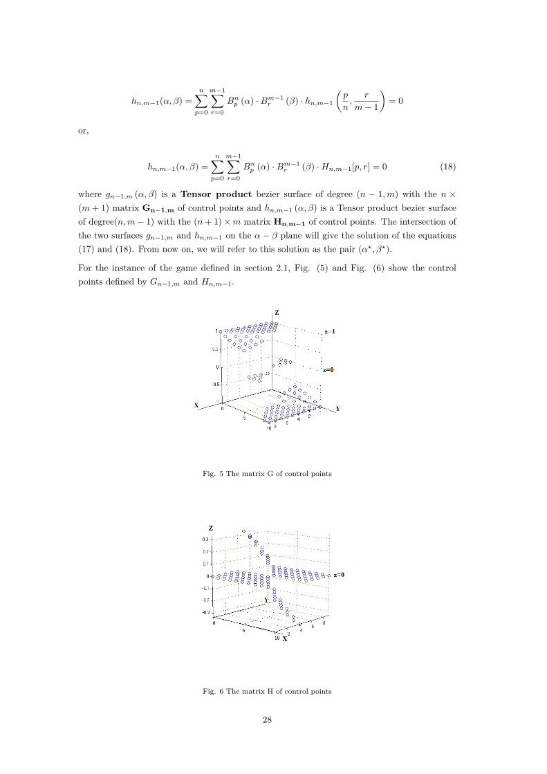
where gn−1,m (α, β) is a Tensor product bezier surface of degree (n − 1,m) with the n ×(m+ 1) matrix Gn−1,m of control points and hn,m−1 (α, β) is a Tensor product bezier surfaceof degree(n,m− 1) with the (n+ 1)×m matrix Hn,m−1 of control points. The intersection ofthe two surfaces gn−1,m and hn,m−1 on the α− β plane will give the solution of the equations(17) and (18). From now on, we will refer to this solution as the pair (α?, β?).

For the instance of the game defined in section 2.1, Fig. (5) and Fig. (6) show the controlpoints defined by Gn−1,m and Hn,m−1.

Fig. 5 The matrix G of control points

Fig. 6 The matrix H of control points

28

6.2 Existence of mixed strategy equilibrium

In this section, we shall investigate into the existence of a solution to the system of Equations(17) and (18).

As we know, a tensor product bezier surface of degrees (m,n) given by (m+1)× (n+1) matrixP of control points is defined as f : I2 → R3 such that:

f(u, v) =m∑i=0

n∑j=0

P [i, j] ·Bmi (u) ·Bmj (v)

We now examine some of the properties of the tensor-product surfaces [2]. Firstly, at u = 0,we have Bmi (u) = 0 for i > 0, and thus C(0, ∗) =

∑nj=0 P [0, j]Bnj (v). Thus this isoparametric

curve is a bezier curve with control points given by the first (or rather 0-th) row of the matrixP. Similarly, C(1, ∗),C(∗, 0) and C(∗, 1) are all bezier and their control points are easily workedout to be the last row, first column, and last column, respectively, of P.

The general isoparametric curve is only a bit more interesting: For a fixed u0 ∈ R, we have

f(u0, v) =n∑j=0

(m∑i=0

P [i, j] ·Bmi (u0)) ·Bmj (v)

In other words, the curve is a bezier curve in v of degree n, with the (n + 1) control points,(q0(u0), . . . , qn(u0)), with qj itself following a bezier curve in u of degree m with control points(P [0, j], . . . , P [m, j]). Thus, we may say that the tensor-product surface is obtained as a fam-ily of bezier curves whose control points move together along ‘rails’ defined by bezier curvesthemselves. Fig. 7 shows the isoparametric curves on a bezier surface.

Fig. 7 Tensor-product Bezier surface ans its isoparametric curves

We shall now visualize the isoparametric curves parallel to Y − Z plane for gn−1,m. For allc ∈

{0, 1

n−1 ,2

n−1 , . . . , 1}, the plane x = c contains the control points (qr (c))r∈{0,1,...,m} defined

as qr(c) =∑n−1i=0 B

n−1i (c) · Gn−1,m[i, r]. These control points define the isoparametric curve

gn−1,m(c, β) (0≤ β ≤ 1). These control points are shown in Fig. 8 for the same game instanceas in section 2.1.

29

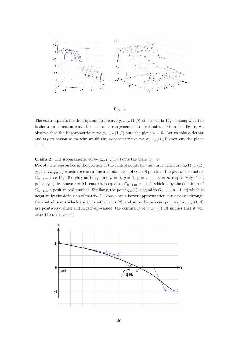
Fig. 8

The control points for the isoparametric curve gn−1,m(1, β) are shown in Fig. 9 along with thebezier approximation curve for such an arrangement of control points. From this figure, weobserve that the isoparametric curve gn−1,m(1, β) cuts the plane z = 0. Let us take a detourand try to reason as to why would the isoparametric curve gn−1,m(1, β) even cut the planez = 0.

Claim 2: The isoparametric curve gn−1,m(1, β) cuts the plane z = 0.Proof: The reason lies in the position of the control points for this curve which are q0(1), q1(1),q2(1), . . ., qm(1) which are each a linear combination of control points in the plot of the matrixGn−1,m (see Fig. 5) lying on the planes y = 0, y = 1, y = 2, . . ., y = m respectively. Thepoint q0(1) lies above z = 0 because it is equal to Gn−1,m[n− 1, 0] which is by the definition ofGn−1,m a positive real number. Similarly, the point qm(1) is equal to Gn−1,m[n−1,m] which isnegative by the definition of matrix G. Now, since a bezier approximation curve passes throughthe control points which are at its either ends [2], and since the two end points of gn−1,m(1, β)are positively-valued and negatively-valued, the continuity of gn−1,m(1, β) implies that it willcross the plane z = 0.

30

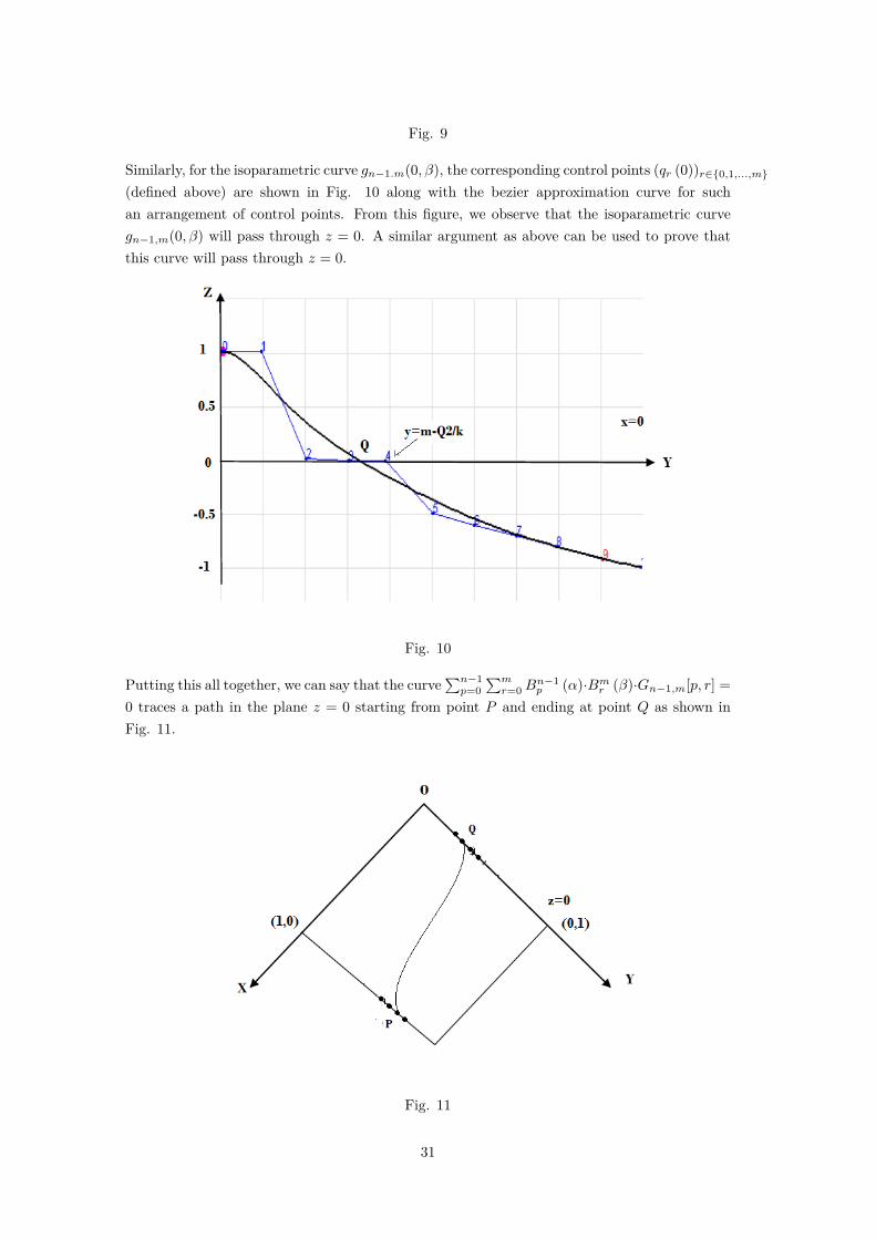
Fig. 9

Similarly, for the isoparametric curve gn−1.m(0, β), the corresponding control points (qr (0))r∈{0,1,...,m}(defined above) are shown in Fig. 10 along with the bezier approximation curve for suchan arrangement of control points. From this figure, we observe that the isoparametric curvegn−1,m(0, β) will pass through z = 0. A similar argument as above can be used to prove thatthis curve will pass through z = 0.

Fig. 10

Putting this all together, we can say that the curve∑n−1p=0

∑mr=0B

n−1p (α)·Bmr (β)·Gn−1,m[p, r] =

0 traces a path in the plane z = 0 starting from point P and ending at point Q as shown inFig. 11.

Fig. 11

31

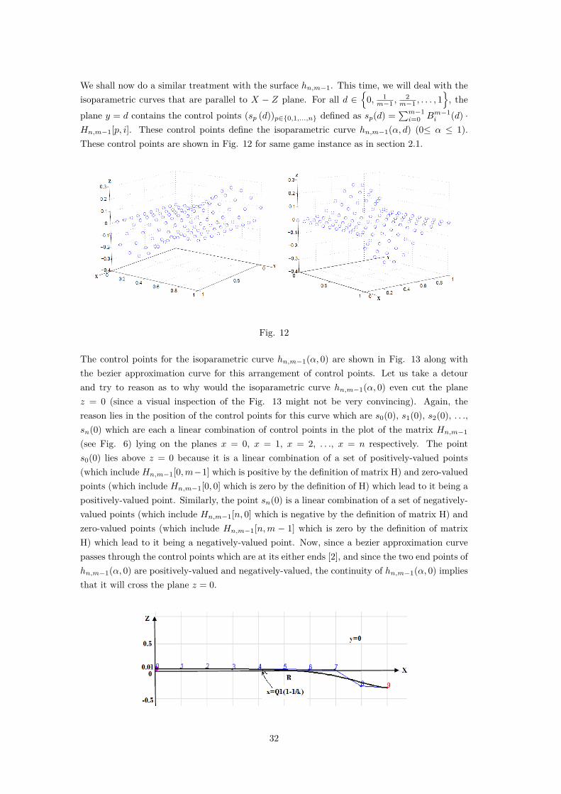
We shall now do a similar treatment with the surface hn,m−1. This time, we will deal with theisoparametric curves that are parallel to X − Z plane. For all d ∈

{0, 1

m−1 ,2

m−1 , . . . , 1}, the

plane y = d contains the control points (sp (d))p∈{0,1,...,n} defined as sp(d) =∑m−1i=0 Bm−1

i (d) ·Hn,m−1[p, i]. These control points define the isoparametric curve hn,m−1(α, d) (0≤ α ≤ 1).These control points are shown in Fig. 12 for same game instance as in section 2.1.

Fig. 12

The control points for the isoparametric curve hn,m−1(α, 0) are shown in Fig. 13 along withthe bezier approximation curve for this arrangement of control points. Let us take a detourand try to reason as to why would the isoparametric curve hn,m−1(α, 0) even cut the planez = 0 (since a visual inspection of the Fig. 13 might not be very convincing). Again, thereason lies in the position of the control points for this curve which are s0(0), s1(0), s2(0), . . .,sn(0) which are each a linear combination of control points in the plot of the matrix Hn,m−1

(see Fig. 6) lying on the planes x = 0, x = 1, x = 2, . . ., x = n respectively. The points0(0) lies above z = 0 because it is a linear combination of a set of positively-valued points(which include Hn,m−1[0,m−1] which is positive by the definition of matrix H) and zero-valuedpoints (which include Hn,m−1[0, 0] which is zero by the definition of H) which lead to it being apositively-valued point. Similarly, the point sn(0) is a linear combination of a set of negatively-valued points (which include Hn,m−1[n, 0] which is negative by the definition of matrix H) andzero-valued points (which include Hn,m−1[n,m − 1] which is zero by the definition of matrixH) which lead to it being a negatively-valued point. Now, since a bezier approximation curvepasses through the control points which are at its either ends [2], and since the two end points ofhn,m−1(α, 0) are positively-valued and negatively-valued, the continuity of hn,m−1(α, 0) impliesthat it will cross the plane z = 0.

32

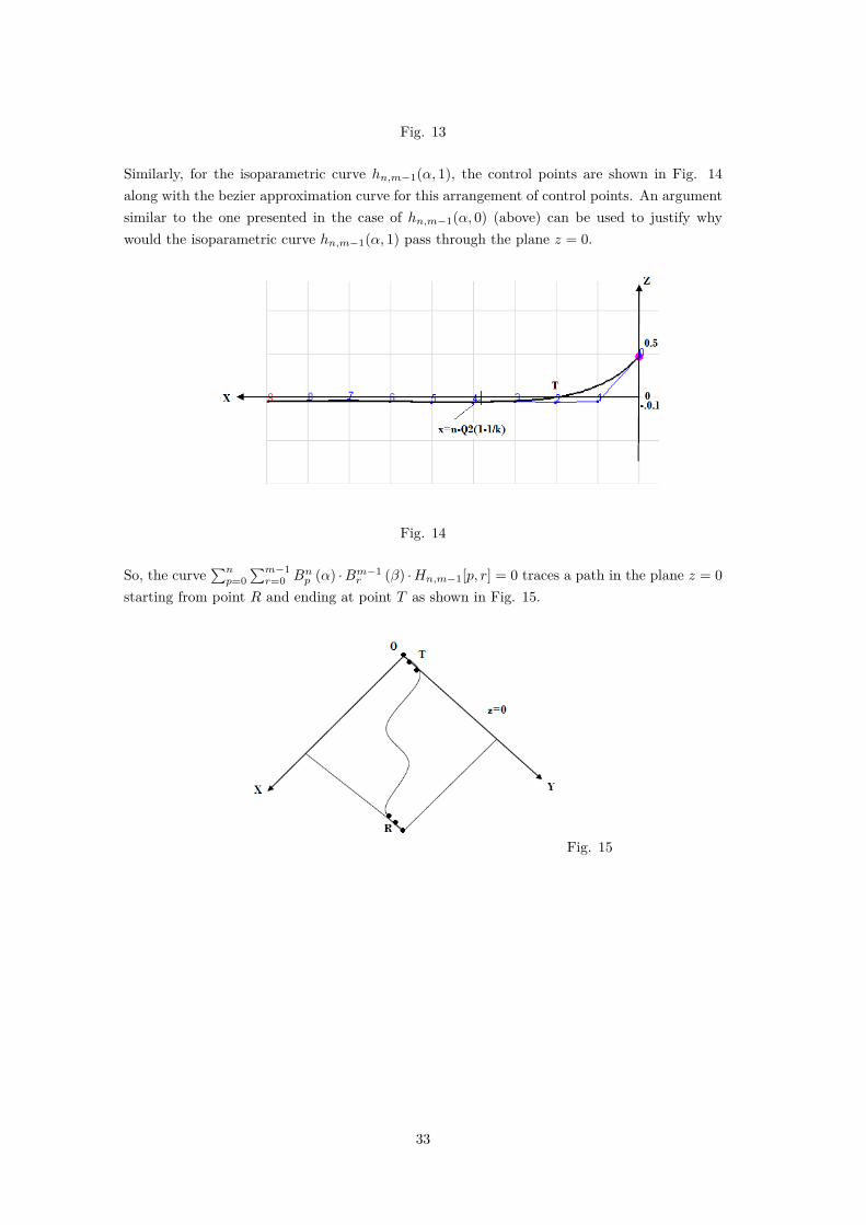
Fig. 13

Similarly, for the isoparametric curve hn,m−1(α, 1), the control points are shown in Fig. 14along with the bezier approximation curve for this arrangement of control points. An argumentsimilar to the one presented in the case of hn,m−1(α, 0) (above) can be used to justify whywould the isoparametric curve hn,m−1(α, 1) pass through the plane z = 0.

Fig. 14

So, the curve∑np=0

∑m−1r=0 Bnp (α) ·Bm−1

r (β) ·Hn,m−1[p, r] = 0 traces a path in the plane z = 0starting from point R and ending at point T as shown in Fig. 15.

Fig. 15

33

Fig. 16 shows all the results of the above analysis

Fig. 16

Claim 3: In the figure above (Fig. 16) , the two curves, one with end-points P and Q (call itC1) and the other with end-points R and T (call it C2), will intersect.

Proof: The curve C1 divides the unit square into two closed parts. The two end points of thecurve C2 lie in the either of the two partitions. So, C2 being continuous will trace a path inz = 0 which will have to move from one partition to another. The point at which C2 crossesthe boundary of these partitions will be its point of intersection with C1 also.

Notice that in the preceding analysis, we have proved that the two curves gn−1,m and hn,m−1

have their end points on the lines x = 0,x = 1 and y = 0,y = 1 respectively due to this theyhave a unique solution. Thus, there exists a solution to the randomized strategy equilibriumin which all the poor buyers choose between the two vendors with the same probability α? andall the rich buyers choose between the two vendors with the same probability β?.

34

6.3 A trivial mixed strategy equilibrium

From now on, we shall consider the two vendors to be identical in the sense that they bothhave the same quantity of commodity (viz. Q1 = Q2 = Q⇒ X1 = X2 and Y1 = Y2).

Till now, we have proved the existence of a randomized strategy for the game. A moment’sreflection will make it clear that α = 1

2 and β = 12 is a point of intersection of gn−1,m (α, β) = 0

and hn,m−1 (α, β) = 0. Below is a formal proof for this.

Claim: α = 12 and β = 1

2 is a solution to the system of Equations (17) and (18).

Proof: Substituting α = 12 and β = 1

2 in Equation (17), we get:

n−1∑p=0

m∑r=0

Bn−1p

(12

)·Bmr

(12

)·G[p, r] = gn−1,m

(12,12

)

=(

12

)n+m−1·n−1∑p=0

m∑r=0

(n− 1r

)·(m

r

)· (x (p+ 1, r)− x (n− p,m− r))

=(

12

)n+m−1

∑mr=0

(n−1

0)·(mr

)· (x (1, r)− x (n,m− r))

+∑mr=0

(n−1

1)·(mr

)· (x (2, r)− x (n− 1,m− r))

+...

+∑mr=0

(n−1n−2)·(mr

)· (x (n− 1, r)− x (2,m− r))

+∑mr=0

(n−1n−1)·(mr

)· (x (n, r)− x (1,m− r))

(19)

The jth summation and the (n− 1− j)th summation (0 ≤ j ≤ n− 1) in the above summationof summations add up to zero as shown below:

m∑r=0

(n− 1j

)·(mr

)· (x (j + 1, r)− x (n− j,m− r)) +

m∑r=0

( n− 1n− 1− j

)·(mr

)· (x (n− j, r)− x (j + 1,m− r))

=(n−1j

)·{∑m

r=0

(mr

)· (x (j + 1, r)− x (n− j,m− r)) +

∑m

r=0

(mr

)· (x (n− j, r)− x (j + 1,m− r))

} (as(n−1j

)=(n−1n−1−j

))

=(n− 1

j

)·

[ (m0

)· (x (j + 1, 0)− x (n− j,m)) +

(m1

)· (x (j + 1, 0)− x (n− j,m− 1)) + . . .+

(mm

)· (x (j + 1,m)− x (n− j, 0))(

m0

)· (x (n− j, 0)− x (j + 1,m)) +

(m1

)· (x (n− j, 0)− x (j + 1,m− 1)) + . . .+

(mm

)· (x (n− j,m)− x (j + 1, 0))

]

=(n− 1

j

)· [0 + 0 + 0 + . . .+ 0] (as

(mz

)=( m

m− z

))

In the above summation of summation (equation (19)), if there is a single middle term then itdoes not have an additive inverse in the expression. This would happen if the number of termsis odd i.e. n is odd. The middle term will be corresponding to j = n−1

2 and will be

m∑r=0

(m

r

)·(n− 1n−1

2

)·((

n+ 12

, r

)−(n+ 1

2,m− r

))

35

or,

=(n− 1n−1

2

)·

[ (m0)·(x(n+1

2 , 0)− x

(n+1

2 ,m))

+(m1)·(x(n+1

2 , 0)− x

(n+1

2 ,m− 1))

+ . . .(mm−1

)·(x(n+1

2 ,m− 1)− x

(n+1

2 , 1))

+(mm

)·(x(n+1

2 ,m)− x

(n+1

2 , 0)) ]

= 0(as

(m

r

)=(

m

m− r

))so, the summation of the summation (equation (19)) vanishes. Hence, gn−1,m

( 12 ,

12)

= 0.

Similarly, substituting α = 12 and β = 1

2 in Equation (18) and simplifying on the above lineswe can shown that hn,m−1

( 12 ,

12)

= 0. Hence, (α?, β?) =( 1

2 ,12)is a randomized strategy Nash

equilibrium in which both the rich and poor players choose to go to either of the vendors withequal probability of 1

2 .

6.4 Mixed strategy segmentation in the market

Segmentation in a market is a situation where:

• A set of buyers prefer a particular vendor more than an other vendor and the remainingbuyers prefer the latter more than the former, and

• the trading prices at the vendors are also different.

To prove the first requirement of segmentation we need to prove that there are two moresolutions to gn−1,m (α, β) = 0 and hn,m−1 (α, β) = 0 (henceforth referred to as g = 0 and h = 0respectively) other than α = 1

2 and β = 12 . So, let us try to find out the shapes of the curves

g = 0 and h = 0 which will lead to three points of intersection.

6.4.1 Condition 1

Consider the plot of X[p, r] (the payoff received by the poor players going to V1 when p-poorand r-rich go to vendor V2) and −X[n − p,m − r] (the negative of the payoff received by thepoor players going to V1 when (n−p)-poor and (m−r)-rich go to vendor V2). Notice the pointsA and B in Figure 17. We shall show that the shape of the curves g = 0 and h = 0 are guidedby the “relative positions” of points A and B.

36

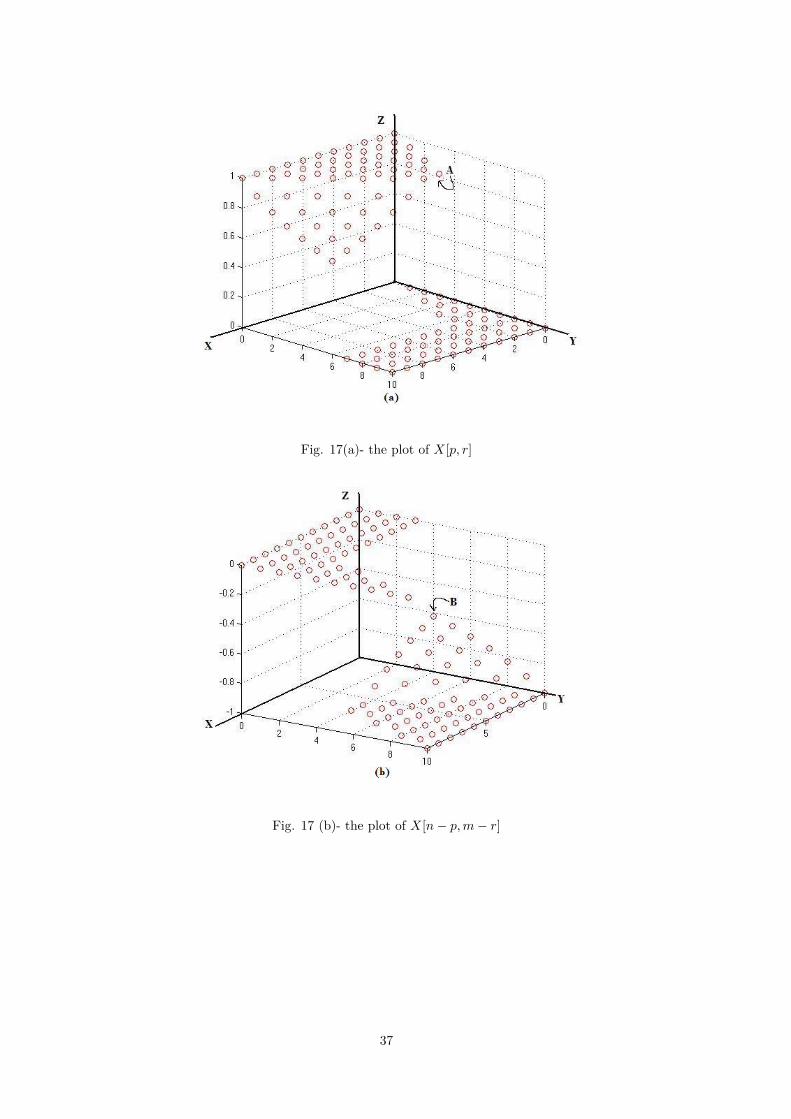
Fig. 17(a)- the plot of X[p, r]

Fig. 17 (b)- the plot of X[n− p,m− r]

37

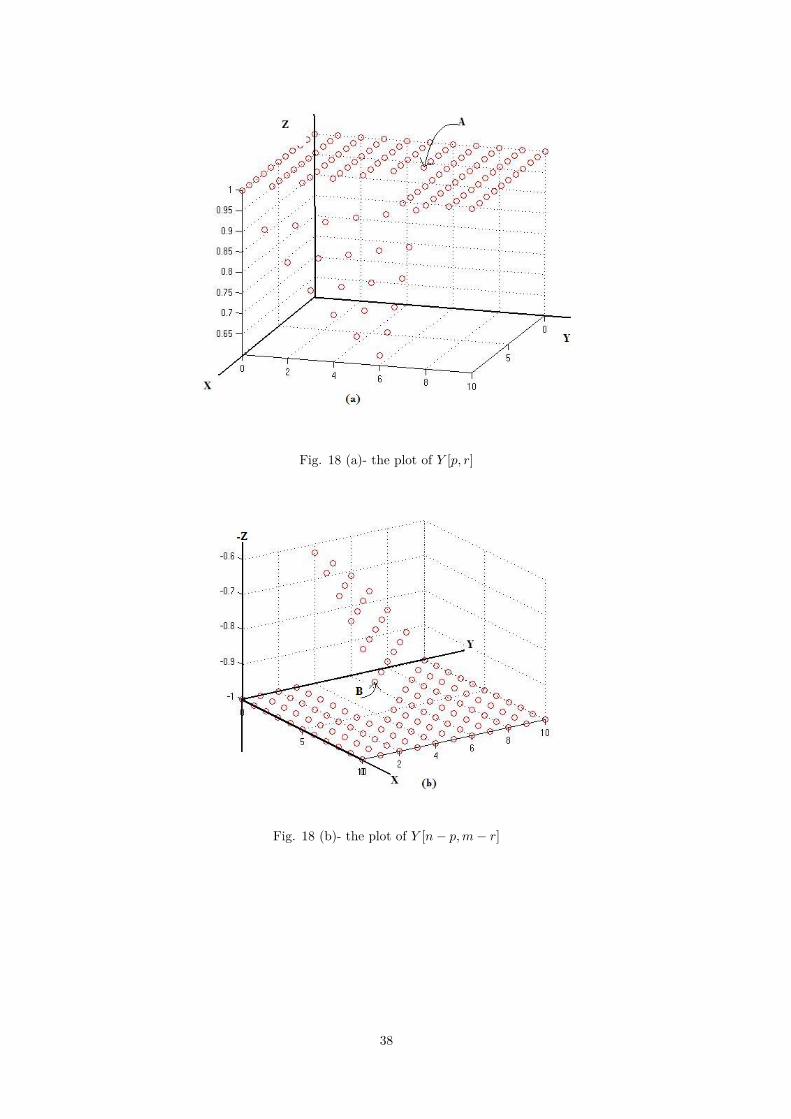
Fig. 18 (a)- the plot of Y [p, r]

Fig. 18 (b)- the plot of Y [n− p,m− r]

38

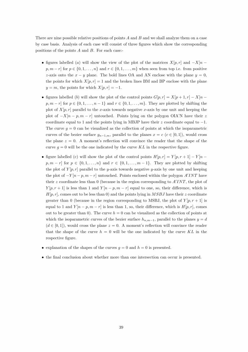
There are nine possible relative positions of points A and B and we shall analyze them on a caseby case basis. Analysis of each case will consist of three figures which show the correspondingpositions of the points A and B. For each case:-

• figures labelled (a) will show the view of the plot of the matrices X[p, r] and −X[n −p,m− r] for p ∈ {0, 1, . . . , n} and r ∈ {0, 1, . . . ,m} when seen from top i.e. from positivez-axis onto the x − y plane. The bold lines OA and AN enclose with the plane y = 0,the points for which X[p, r] = 1 and the broken lines BM and BP enclose with the planey = m, the points for which X[p, r] = −1.

• figures labelled (b) will show the plot of the control points G[p, r] = X[p+ 1, r]−X[n−p,m− r] for p ∈ {0, 1, . . . , n− 1} and r ∈ {0, 1, . . . ,m}. They are plotted by shifting theplot of X[p, r] parallel to the x-axis towards negative x-axis by one unit and keeping theplot of −X[n − p,m − r] untouched. Points lying on the polygon OIA’N have their zcoordinate equal to 1 and the points lying in MBJP have their z coordinate equal to −1.The curve g = 0 can be visualized as the collection of points at which the isoparametriccurves of the bezier surface gn−1,m, parallel to the planes x = c (c ∈ [0, 1]), would crossthe plane z = 0. A moment’s reflection will convince the reader that the shape of thecurve g = 0 will be the one indicated by the curve KL in the respective figure.

• figure labelled (c) will show the plot of the control points H[p, r] = Y [p, r + 1] − Y [n −p,m − r] for p ∈ {0, 1, . . . , n} and r ∈ {0, 1, . . . ,m− 1}. They are plotted by shiftingthe plot of Y [p, r] parallel to the y-axis towards negative y-axis by one unit and keepingthe plot of −Y [n− p,m− r] untouched. Points enclosed within the polygon A′INT havetheir z coordinate less than 0 (because in the region corresponding to A′INT , the plot ofY [p, r + 1] is less than 1 and Y [n − p,m − r] equal to one, so, their difference, which isH[p, r], comes out to be less than 0) and the points lying inMSBJ have their z coordinategreater than 0 (because in the region corresponding to MSBJ, the plot of Y [p, r + 1] isequal to 1 and Y [n− p,m− r] is less than 1, so, their difference, which is H[p, r], comesout to be greater than 0). The curve h = 0 can be visualized as the collection of points atwhich the isoparametric curves of the bezier surface hn,m−1, parallel to the planes y = d

(d ∈ [0, 1]), would cross the plane z = 0. A moment’s reflection will convince the readerthat the shape of the curve h = 0 will be the one indicated by the curve KL in therespective figure.

• explanation of the shapes of the curves g = 0 and h = 0 is presented.

• the final conclusion about whether more than one intersection can occur is presented.

39

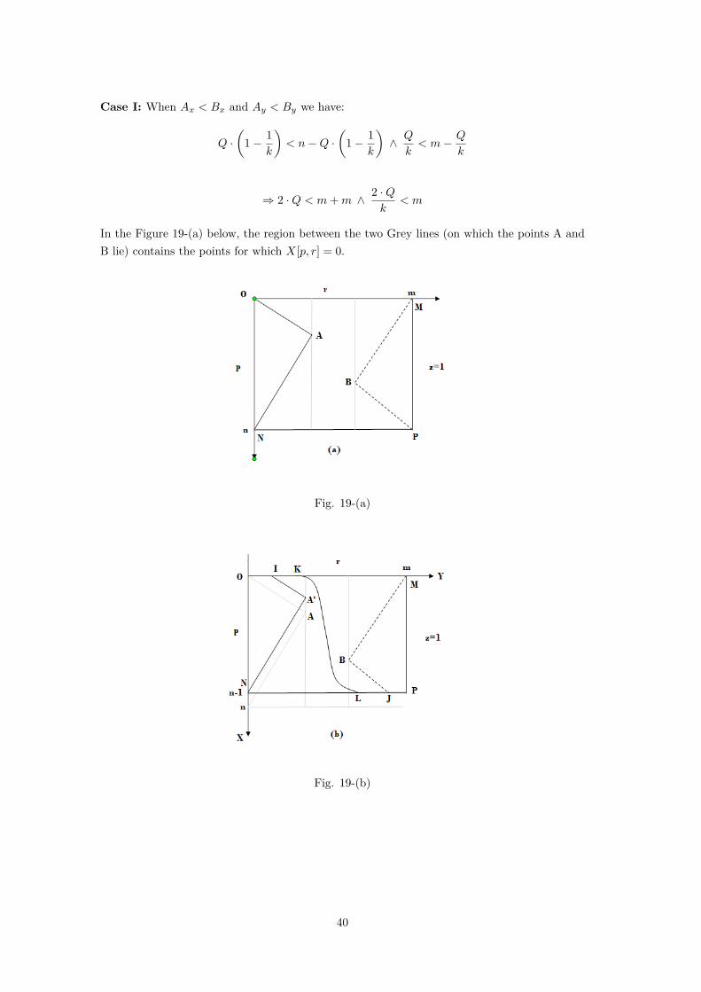
Case I: When Ax < Bx and Ay < By we have:

Q ·(

1− 1k

)< n−Q ·

(1− 1

k

)∧ Q

k< m− Q

k

⇒ 2 ·Q < m+m ∧ 2 ·Qk

< m

In the Figure 19-(a) below, the region between the two Grey lines (on which the points A andB lie) contains the points for which X[p, r] = 0.

Fig. 19-(a)

Fig. 19-(b)

40

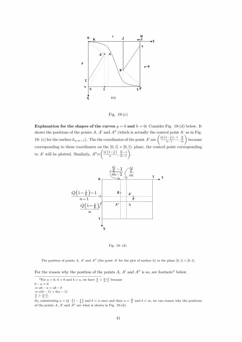
Fig. 19-(c)

Explanation for the shapes of the curves g = 0 and h = 0: Consider Fig. 19-(d) below. Itshows the positions of the points A, A′ and A′′ (which is actually the control point A’ as in Fig.

19- (c) for the surface hn,m−1). The the coordinates of the pointA′ are(Q·(1− 1

k )−1n−1 ,

Qk

m

)because

corresponding to these coordinates on the [0, 1]× [0, 1]- plane, the control point corresponding

to A′ will be plotted. Similarly, A′′≡(Q·(1− 1

k )n ,

Qk −1m−1

).

Fig. 19- (d)

The position of points A, A′ and A′′ (the point A′ for the plot of surface h) in the plane [0, 1]× [0, 1].

For the reason why the position of the points A, A′ and A′′ is so, see footnote4 below.4For a > 0, b > 0 and b > a, we have a

b> a−1b−1 because

b− a > 0⇒ ab− a > ab− b⇒ a(b− 1) > b(a− 1)ab> a−1b−1 .

So, substituting a = Q ·(1− 1

k

)and b = n once and then a = Q

kand b = m, we can reason why the positions

of the points A, A′ and A′′ are what is shown in Fig. 19-(d).

41

The curve g = 0 passes through two points: one on the y-axis (not the origin O), which can bejustified by the general plot of gn−1,m (0, β) in Fig. 10, and the other on the line x = Q·(1− 1

k )−1n−1

and between A′ and the line y = 1, say P . The curve h = 0 passes through the origin O anda point on the line y =

Qk −1m−1 and between the point A′′ and y- axis, say Q. Since the curves

g = 0 and h = 0 are increasing functions (because of the arrangement of the control points),they will not intersect till they are traversed up to the points A′ and A′′. And as we knowthat h = 0 and g = 0 intersect at

( 12 ,

12), the two curves will further not intersect till the reach( 1

2 ,12). A similar argument can be given for the fact that the two curves g = 0 and h = 0 will

not intersect in the region{(x, y) | 12 ≤ x ≤ 1 ∧ 1

2 ≤ y ≤ 1}in the current case.

Conclusion: The curves g = 0 and h = 0 do not intersect at any point other than( 1

2 ,12)in

the current case.

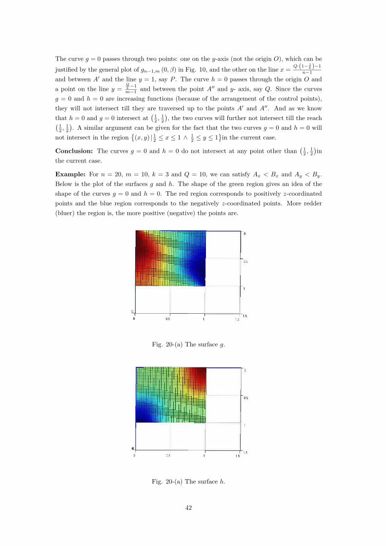
Example: For n = 20, m = 10, k = 3 and Q = 10, we can satisfy Ax < Bx and Ay < By.Below is the plot of the surfaces g and h. The shape of the green region gives an idea of theshape of the curves g = 0 and h = 0. The red region corresponds to positively z-coordinatedpoints and the blue region corresponds to the negatively z-coordinated points. More redder(bluer) the region is, the more positive (negative) the points are.

Fig. 20-(a) The surface g.

Fig. 20-(a) The surface h.

42

The next five cases (listed below) are very much similar to the Case I and reader can easilyverify using examples that the curves g = 0 and h = 0 will not intersect at any point otherthan

( 12 ,

12)in the these cases.

Case II: When Ax = Bx and Ay < By

Case III: When Ax > Bx and Ay < By

Case IV: When Ax < Bx and Ay = By

Case V: When Ax = Bx and Ay = By

Case VI: When Ax > Bx and Ay = By

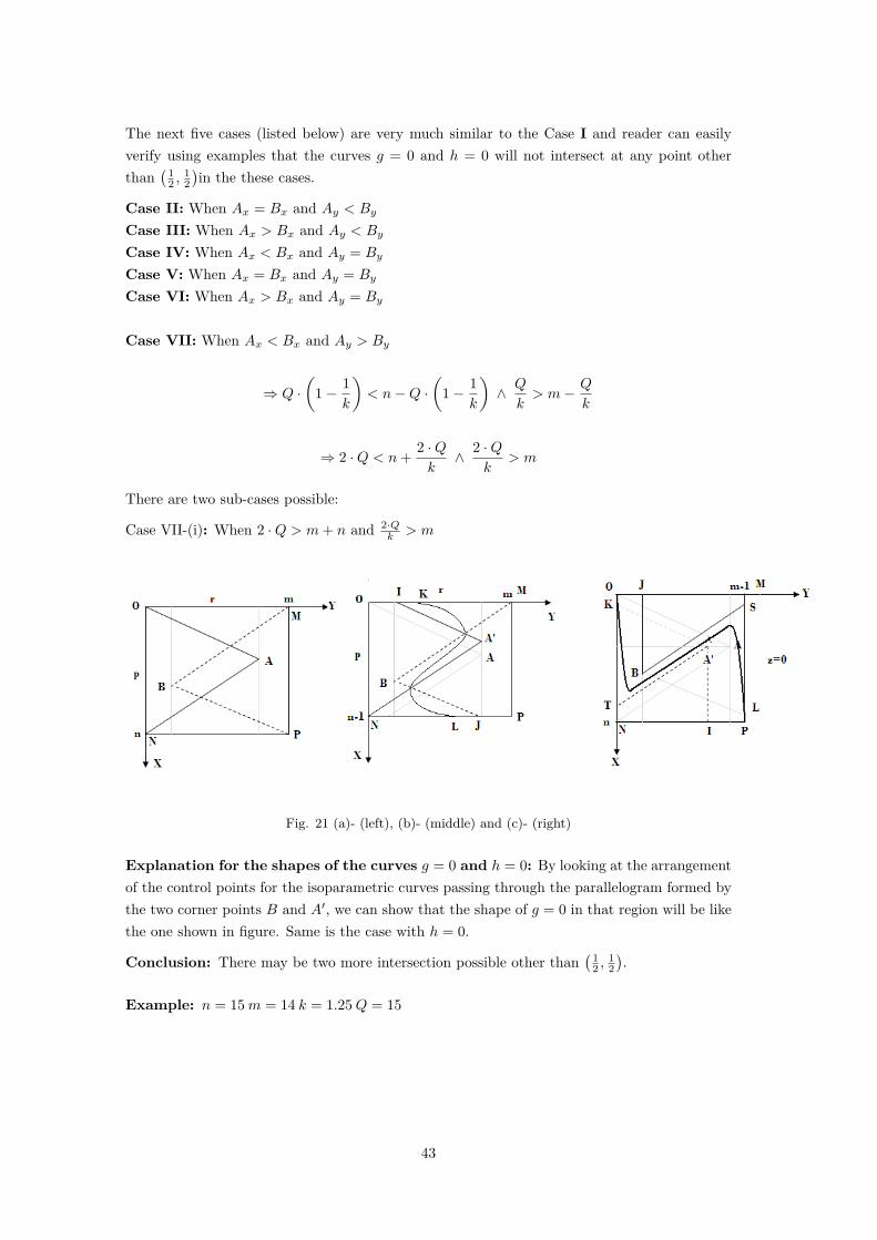
Case VII: When Ax < Bx and Ay > By

⇒ Q ·(

1− 1k

)< n−Q ·

(1− 1

k

)∧ Q

k> m− Q

k

⇒ 2 ·Q < n+ 2 ·Qk∧ 2 ·Q

k> m

There are two sub-cases possible:

Case VII-(i): When 2 ·Q > m+ n and 2·Qk > m

Fig. 21 (a)- (left), (b)- (middle) and (c)- (right)

Explanation for the shapes of the curves g = 0 and h = 0: By looking at the arrangementof the control points for the isoparametric curves passing through the parallelogram formed bythe two corner points B and A′, we can show that the shape of g = 0 in that region will be likethe one shown in figure. Same is the case with h = 0.

Conclusion: There may be two more intersection possible other than( 1

2 ,12).

Example: n = 15m = 14 k = 1.25Q = 15

43

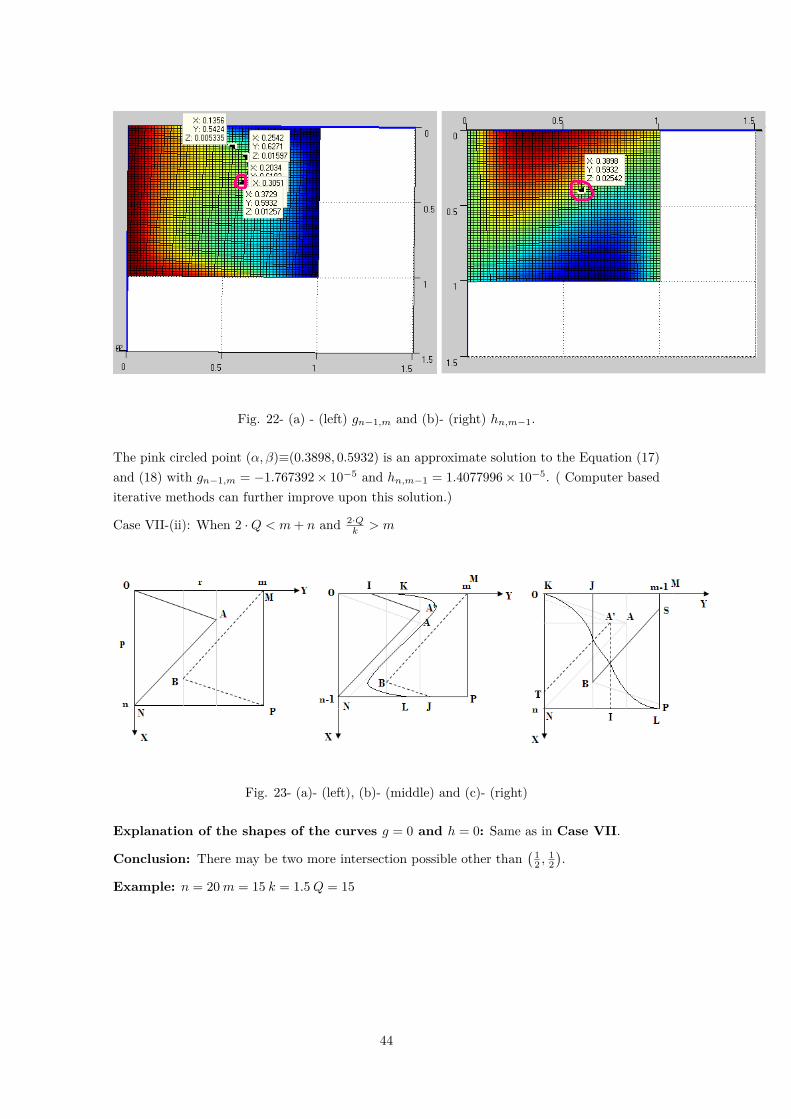
Fig. 22- (a) - (left) gn−1,m and (b)- (right) hn,m−1.

The pink circled point (α, β)≡(0.3898, 0.5932) is an approximate solution to the Equation (17)and (18) with gn−1,m = −1.767392× 10−5 and hn,m−1 = 1.4077996× 10−5. ( Computer basediterative methods can further improve upon this solution.)

Case VII-(ii): When 2 ·Q < m+ n and 2·Qk > m

Fig. 23- (a)- (left), (b)- (middle) and (c)- (right)

Explanation of the shapes of the curves g = 0 and h = 0: Same as in Case VII.


2 ,12).

Example: n = 20m = 15 k = 1.5Q = 15

44

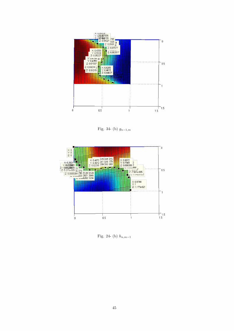
Fig. 34- (b) gn−1,m

Fig. 24- (b) hn,m−1

45

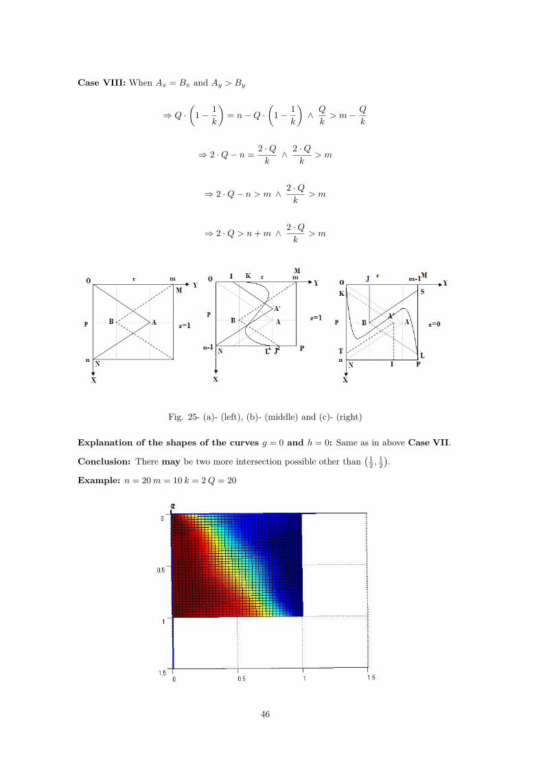
Case VIII: When Ax = Bx and Ay > By

⇒ Q ·(

1− 1k

)= n−Q ·

(1− 1

k

)∧ Q

k> m− Q

k

⇒ 2 ·Q− n = 2 ·Qk∧ 2 ·Q

k> m

⇒ 2 ·Q− n > m ∧ 2 ·Qk

> m

⇒ 2 ·Q > n+m ∧ 2 ·Qk

> m


Explanation of the shapes of the curves g = 0 and h = 0: Same as in above Case VII.


2 ,12).

Example: n = 20m = 10 k = 2Q = 20

46

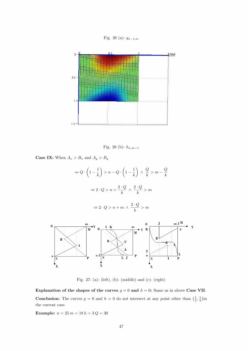
Fig. 26 (a)- gn−1,m

Fig. 26 (b)- hn,m−1

Case IX: When Ax > Bx and Ay > By

⇒ Q ·(

1− 1k

)> n−Q ·

(1− 1

k

)∧ Q

k> m− Q

k

⇒ 2 ·Q > n+ 2 ·Qk∧ 2 ·Q

k> m

⇒ 2 ·Q > n+m ∧ 2 ·Qk

> m


Explanation of the shapes of the curves g = 0 and h = 0: Same as in above Case VII.

Conclusion: The curves g = 0 and h = 0 do not intersect at any point other than( 1

2 ,12)in

the current case.

Example: n = 25m = 18 k = 3Q = 30

47

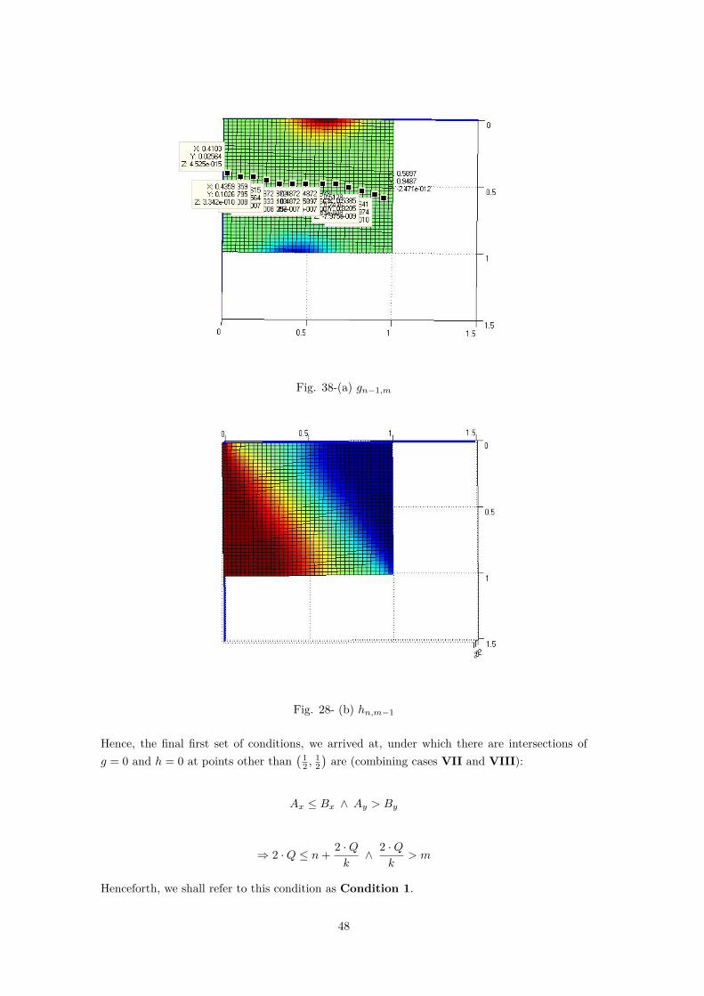
Fig. 38-(a) gn−1,m

Fig. 28- (b) hn,m−1

Hence, the final first set of conditions, we arrived at, under which there are intersections ofg = 0 and h = 0 at points other than

( 12 ,

12)are (combining cases VII and VIII):

Ax ≤ Bx ∧ Ay > By

⇒ 2 ·Q ≤ n+ 2 ·Qk∧ 2 ·Q

k> m

Henceforth, we shall refer to this condition as Condition 1.

48

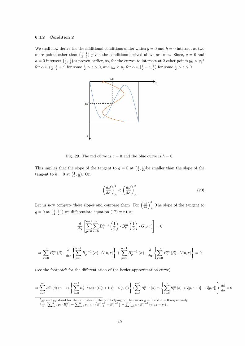
6.4.2 Condition 2

We shall now derive the the additional conditions under which g = 0 and h = 0 intersect at twomore points other than

( 12 ,

12)given the conditions derived above are met. Since, g = 0 and

h = 0 intersect( 1

2 ,12)as proven earlier, so, for the curves to intersect at 2 other points yh > yg

5

for α ∈ ( 12 ,

12 + ε] for some 1

2 > ε > 0, and yh < yg for α ∈ [ 12 − ε,12 ) for some 1

2 > ε > 0.

Fig. 29. The red curve is g = 0 and the blue curve is h = 0.

This implies that the slope of the tangent to g = 0 at( 1

2 ,12)be smaller than the slope of the

tangent to h = 0 at( 1

2 ,12). Or:

(dβ

dα

)gA

<

(dβ

dα

)hA

(20)

Let us now compute these slopes and compare them. For(dβdα

)gA

(the slope of the tangent tog = 0 at

( 12 ,

12)) we differentiate equation (17) w.r.t α:

d

dα

[n−1∑p=0

m∑r=0

Bn−1p

(12

)·Bmr

(12

)·G[p, r]

]= 0

⇒m∑r=0

Bmr (β) · ddα

{n−1∑p=0

Bn−1p (α) ·G[p, r]

}+n−1∑p=0

Bn−1p (α) · d

dα

{m∑r=0

Bmr (β) ·G[p, r]

}= 0

(see the footnote6 for the differentiation of the bezier approximation curve)

⇒m∑r=0

Bmr (β)·(n− 1)·

{n−2∑p=0

Bn−2p (α) · (G[p+ 1, r]−G[p, r])

}+n−1∑p=0

Bn−1p (α)·m·

{m∑r=0

Bmr (β) · (G[p, r + 1]−G[p, r])

}·dβ

dα= 0

5yg and yh stand for the ordinates of the points lying on the curves g = 0 and h = 0 respectively.6 ddx

[∑n

i=0 pi ·Bni

]=∑n

i=0 pi · n ·(Bn−1i−1 −B

n−1i

)=∑n

i=0 n ·Bn−1i (pi+1 − pi) .

49

⇒ (n− 1)·m∑r=0

n−2∑p=0

Bn−2p (α)·Bmr (β)·(G[p+ 1, r]−G[p, r])+m·

n−1∑p=0

m−1∑r=0

Bn−1p (α)·Bm−1

r (β)·(G[p, r + 1]−G[p, r]))·dβ

dα= 0

Substituting α = 12 and β = 1

2 in the above expression gives:

(n− 1)·m∑r=0

n−2∑p=0

(m

r

)·(n− 2p

)·(G[p+ 1, r]−G[p, r])+m·

n−1∑p=0

m−1∑r=0

(n− 1p

)·(m− 1r

)·(G[p, r + 1]−G[p, r]))·dβ

dα= 0

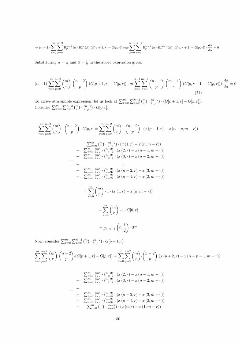
(21)

To arrive at a simple expression, let us look at∑mr=0

∑n−2p=0

(mr

)·(n−2p

)· (G[p+ 1, r]−G[p, r]).

Consider∑mr=0

∑n−2p=0

(mr

)·(n−2p

)·G[p, r]:

m∑r=0

n−2∑p=0

(m

r

)·(n− 2p

)·G[p, r] =

m∑r=0

n−2∑p=0

(m

r

)·(n− 2p

)· (x (p+ 1, r)− x (n− p,m− r))

=

∑mr=0

(mr

)·(n−2

0)· (x (1, r)− x (n,m− r))

+∑mr=0

(mr

)·(n−2

1)· (x (2, r)− x (n− 1,m− r))

+∑mr=0

(mr

)·(n−2

2)· (x (3, r)− x (n− 2,m− r))

+...

+∑mr=0

(mr

)·(n−2n−3)· (x (n− 2, r)− x (3,m− r))

+∑mr=0

(mr

)·(n−2n−2)· (x (n− 1, r)− x (2,m− r))

=m∑r=0

(m

r

)· 1 · (x (1, r)− x (n,m− r))

=m∑r=0

(m

r

)· 1 ·G[0, r]

= gn,m−1

(0, 1

2

)· 2m

Now, consider∑mr=0

∑n−2p=0

(mr

)·(n−2p

)·G[p+ 1, r]:

m∑r=0

n−2∑p=0

(m

r

)·(n− 2p

)·(G[p+ 1, r]−G[p, r]) =

m∑r=0

n−2∑p=0

(m

r

)·(n− 2p

)·(x (p+ 2, r)− x (n− p− 1,m− r))

=

∑mr=0

(mr

)·(n−2

0)· (x (2, r)− x (n− 1,m− r))

+∑mr=0

(mr

)·(n−2

1)· (x (3, r)− x (n− 2,m− r))

+...

+∑mr=0

(mr

)·(n−2n−4)· (x (n− 2, r)− x (3,m− r))

+∑mr=0

(mr

)·(n−2n−3)· (x (n− 1, r)− x (2,m− r))

+∑mr=0

(mr

)·(n−2n−2)· (x (n, r)− x (1,m− r))

50

=m∑r=0

(m

r

)· 1 · (x (n, r)− x (1,m− r))

=m∑r=0

(m

r

)· 1 ·G[n− 1, r]

= gn,m−1

(1, 1

2

)· 2m

Now, since∑mr=0

(mr

)· 1 · (x (1, r)− x (n,m− r)) +

∑mr=0

(mr

)· 1 · (x (n, r)− x (1,m− r)) = 0,

we have:

∑mr=0

(mr

)· 1 · (x (n, r)− x (1,m− r)) +

∑mr=0

(mr

)· 1 · (x (1, r)− x (n,m− r))

= −2 ·∑mr=0

(mr

)· 1 · (x (1, r)− x (1n,m− r))

= −2 · gn−1,m

(0, 1

2

)· 2m

⇒m∑r=0

n−2∑p=0

(m

r

)·(n− 2p

)· (G[p+ 1, r]−G[p, r]) = −2 · gn−1,m

(0, 1

2

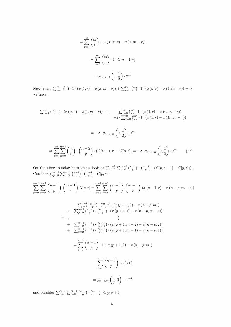
)· 2m (22)

On the above similar lines let us look at∑n−1p=0

∑m−1r=0

(n−1p

)·(m−1r

)· (G[p, r + 1]−G[p, r])).

Consider∑n−1p=0

∑m−1r=0

(n−1p

)·(m−1r

)·G[p, r]:

n−1∑p=0

m−1∑r=0

(n− 1p

)·(m− 1r

)·G[p, r] =

n−1∑p=0

m−1∑r=0

(n− 1p

)·(m− 1r

)·(x (p+ 1, r)− x (n− p,m− r))

=

∑n−1p=0

(n−1p

)·(m−1

0)· (x (p+ 1, 0)− x (n− p,m))

+∑n−1p=0

(n−1p

)·(m−1

1)· (x (p+ 1, 1)− x (n− p,m− 1))

+...

+∑n−1p=0

(n−1p

)·(m−1m−2

)· (x (p+ 1,m− 2)− x (n− p, 2))

+∑n−1p=0

(n−1p

)·(m−1m−1

)· (x (p+ 1,m− 1)− x (n− p, 1))

=n−1∑p=0

(n− 1p

)· 1 · (x (p+ 1, 0)− x (n− p,m))

=n−1∑p=0

(n− 1p

)·G[p, 0]

= gn−1,m

(12, 0)· 2n−1

and consider∑n−1p=0

∑m−1r=0

(n−1p

)·(m−1r

)·G[p, r + 1]:

51

n−1∑p=0

m−1∑r=0

(n− 1p

)·(m− 1r

)·G[p, r+1] =

n−1∑p=0

m−1∑r=0

(n− 1p

)·(m− 1r

)·(x (p+ 1, r + 1)− x (n− p,m− r − 1))

=

∑n−1p=0

(n−1p

)·(m−1

0)· (x (p+ 1, 1)− x (n− p,m− 1))

+∑n−1p=0

(n−1p

)·(m−1

1)· (x (p+ 1, 2)− x (n− p,m− 2))

+...

+∑n−1p=0

(n−1p

)·(m−1m−2

)· (x (p+ 1,m− 1)− x (n− p, 1))

+∑n−1p=0

(n−1p

)·(m−1m−1

)· (x (p+ 1,m)− x (n− p, 0))

=n−1∑p=0

(n− 1p

)· 1 · (x (p+ 1,m)− x (n− p, 0))

=n−1∑p=0

(n− 1p

)·G[p,m]

= gn−1,m

(12, 1)· 2n−1

Now, since∑n−1p=0

(n−1p

)·1·(x (p+ 1,m)− x (n− p, 0))+

∑n−1p=0

(n−1p

)·1·(x (p+ 1, 0)− x (n− p,m)) =

0

⇒∑n−1p=0

(n−1p

)· 1 · (x (p+ 1,m)− x (n− p, 0)) −

∑n−1p=0

(n−1p

)· 1 · (x (p+ 1, 0)− x (n− p,m))

= −2 ·∑n−1p=0

(n−1p

)· 1 · (x (p+ 1, 0)− x (n− p,m))

or,

n−1∑p=0

m−1∑r=0

(n− 1p

)·(m− 1r

)·(G[p, r + 1]−G[p, r])) = −2·

n−1∑p=0

(n− 1p

)·1·(x (p+ 1, 0)− x (n− p,m))

= −2 · gn−1,m

(12, 0)· 2n−1

⇒n−1∑p=0

m−1∑r=0

(n− 1p

)·(m− 1r

)· (G[p, r + 1]−G[p, r])) = −2 · gn−1,m

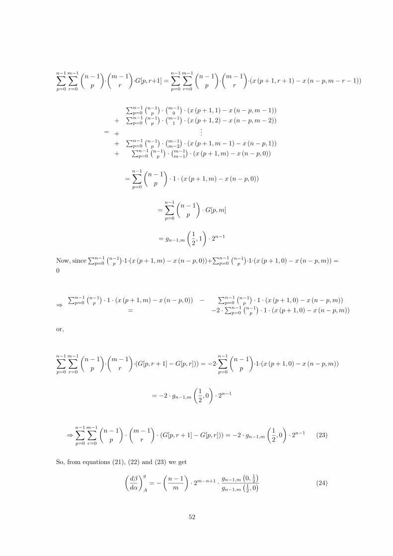
(12, 0)· 2n−1 (23)

So, from equations (21), (22) and (23) we get(dβ

dα

)gA

= −(n− 1m

)· 2m−n+1 ·

gn−1,m(0, 1

2)

gn−1,m( 1

2 , 0) (24)

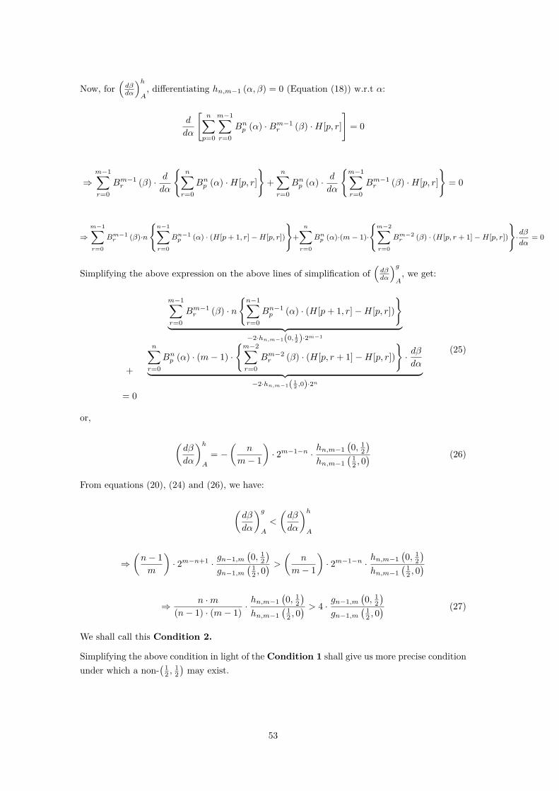
52

Now, for(dβdα

)hA, differentiating hn,m−1 (α, β) = 0 (Equation (18)) w.r.t α:

d

dα

[n∑p=0

m−1∑r=0

Bnp (α) ·Bm−1r (β) ·H[p, r]

]= 0

⇒m−1∑r=0

Bm−1r (β) · d

dα

{n∑r=0

Bnp (α) ·H[p, r]

}+

n∑r=0

Bnp (α) · ddα

{m−1∑r=0

Bm−1r (β) ·H[p, r]

}= 0

⇒m−1∑r=0

Bm−1r (β)·n

{n−1∑r=0

Bn−1p (α) · (H[p+ 1, r]−H[p, r])

}+n∑r=0

Bnp (α)·(m− 1)·

{m−2∑r=0

Bm−2r (β) · (H[p, r + 1]−H[p, r])

}·dβ

dα= 0

Simplifying the above expression on the above lines of simplification of(dβdα

)gA, we get:

m−1∑r=0

Bm−1r (β) · n

{n−1∑r=0

Bn−1p (α) · (H[p+ 1, r]−H[p, r])

}︸︷︷︸

−2·hn,m−1(0, 12 )·2m−1

+

n∑r=0

Bnp (α) · (m− 1) ·

{m−2∑r=0

Bm−2r (β) · (H[p, r + 1]−H[p, r])

}· dβdα︸︷︷︸

−2·hn,m−1( 12 ,0)·2n

= 0

(25)

or,

(dβ

dα

)hA

= −(

n

m− 1

)· 2m−1−n ·

hn,m−1(0, 1

2)

hn,m−1( 1

2 , 0) (26)

From equations (20), (24) and (26), we have:

(dβ

dα

)gA

<

(dβ

dα

)hA

⇒(n− 1m

)· 2m−n+1 ·

gn−1,m(0, 1

2)

gn−1,m( 1

2 , 0) > ( n

m− 1

)· 2m−1−n ·

hn,m−1(0, 1

2)

hn,m−1( 1

2 , 0)

⇒ n ·m(n− 1) · (m− 1)

·hn,m−1

(0, 1

2)

hn,m−1( 1

2 , 0) > 4 ·

gn−1,m(0, 1

2)

gn−1,m( 1

2 , 0) (27)

We shall call this Condition 2.

Simplifying the above condition in light of the Condition 1 shall give us more precise conditionunder which a non-

( 12 ,

12)may exist.

53

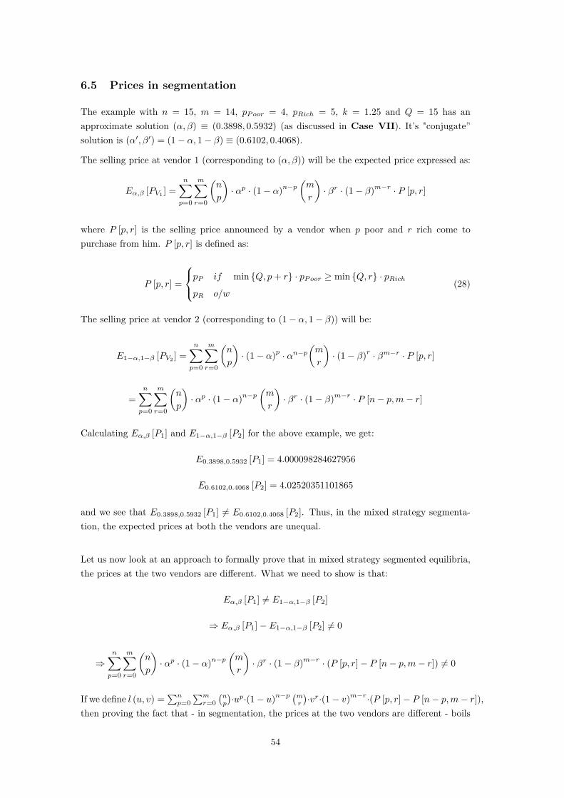
6.5 Prices in segmentation

The example with n = 15, m = 14, pPoor = 4, pRich = 5, k = 1.25 and Q = 15 has anapproximate solution (α, β) ≡ (0.3898, 0.5932) (as discussed in Case VII). It’s "conjugate”solution is (α′, β′) = (1− α, 1− β) ≡ (0.6102, 0.4068).

The selling price at vendor 1 (corresponding to (α, β)) will be the expected price expressed as:

Eα,β [PV1 ] =n∑p=0

m∑r=0

(n

p

)· αp · (1− α)n−p

(m

r

)· βr · (1− β)m−r · P [p, r]

where P [p, r] is the selling price announced by a vendor when p poor and r rich come topurchase from him. P [p, r] is defined as:

P [p, r] =

pP if min {Q, p+ r} · pPoor ≥ min {Q, r} · pRichpR o/w

(28)

The selling price at vendor 2 (corresponding to (1− α, 1− β)) will be:

E1−α,1−β [PV2 ] =n∑p=0

m∑r=0

(n

p

)· (1− α)p · αn−p

(m

r

)· (1− β)r · βm−r · P [p, r]

=n∑p=0

m∑r=0

(n

p

)· αp · (1− α)n−p

(m

r

)· βr · (1− β)m−r · P [n− p,m− r]

Calculating Eα,β [P1] and E1−α,1−β [P2] for the above example, we get:

E0.3898,0.5932 [P1] = 4.000098284627956

E0.6102,0.4068 [P2] = 4.02520351101865

and we see that E0.3898,0.5932 [P1] 6= E0.6102,0.4068 [P2]. Thus, in the mixed strategy segmenta-tion, the expected prices at both the vendors are unequal.

Let us now look at an approach to formally prove that in mixed strategy segmented equilibria,the prices at the two vendors are different. What we need to show is that:

Eα,β [P1] 6= E1−α,1−β [P2]

⇒ Eα,β [P1]− E1−α,1−β [P2] 6= 0

⇒n∑p=0

m∑r=0

(n

p

)· αp · (1− α)n−p

(m

r

)· βr · (1− β)m−r · (P [p, r]− P [n− p,m− r]) 6= 0

If we define l (u, v) =∑np=0

∑mr=0

(np

)·up·(1− u)n−p

(mr

)·vr·(1− v)m−r·(P [p, r]− P [n− p,m− r]),

then proving the fact that - in segmentation, the prices at the two vendors are different - boils

54

down to proving that l (α1, β1) 6= 0. Notice that l (α1, β1) is again a bezier surface with controlpoints J [p, r] = P [p, r]− P [n− p,m− r] (0 ≤ p ≤ n and 0 ≤ r ≤ m).

It can be shown by direct substitution that l( 12 ,

12 ) = 0. Also, under the conditions in which we

expect segmentation to occur, a typical plot of control points looks like:-

Fig. 30.

In the regions OVU, UMSN and SWH, J = 0. The region containing ” + ” sign contains positive J(= pR − pP )

and the region containing ”− ” sign contains the negative J(= pP − pR). The red lines AG and CE are x = 12

and y = 12 respectively.

For the example considered above (i.e. under the conditions in which we expect segmentationto occur), the plot of the control points J [p, r] and the bezier surface l (α, β) are shown below:

Fig. 31 The control points J [p, r]

55

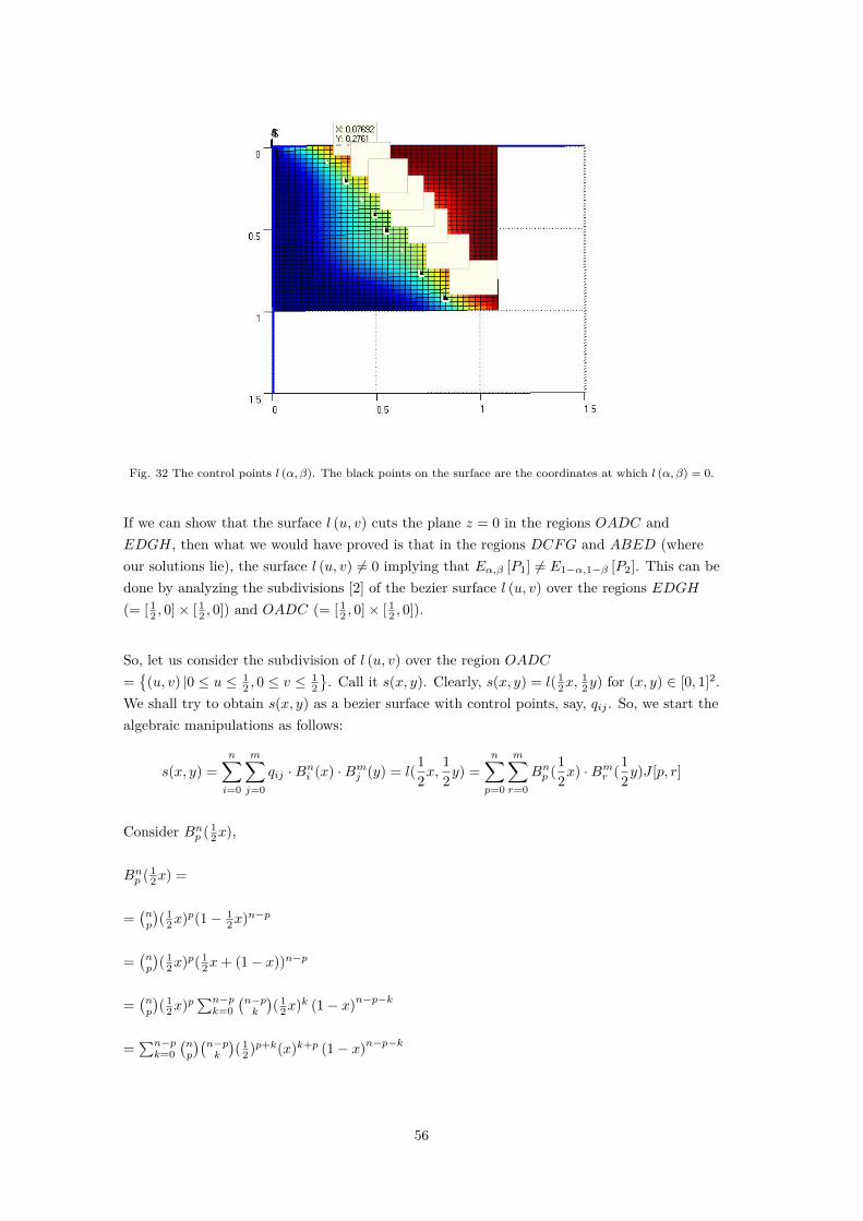
Fig. 32 The control points l (α, β). The black points on the surface are the coordinates at which l (α, β) = 0.

If we can show that the surface l (u, v) cuts the plane z = 0 in the regions OADC andEDGH, then what we would have proved is that in the regions DCFG and ABED (whereour solutions lie), the surface l (u, v) 6= 0 implying that Eα,β [P1] 6= E1−α,1−β [P2]. This can bedone by analyzing the subdivisions [2] of the bezier surface l (u, v) over the regions EDGH(= [ 12 , 0]× [ 12 , 0]) and OADC (= [ 12 , 0]× [ 12 , 0]).

So, let us consider the subdivision of l (u, v) over the region OADC={(u, v) |0 ≤ u ≤ 1

2 , 0 ≤ v ≤12}. Call it s(x, y). Clearly, s(x, y) = l( 1

2x,12y) for (x, y) ∈ [0, 1]2.

We shall try to obtain s(x, y) as a bezier surface with control points, say, qij . So, we start thealgebraic manipulations as follows:

s(x, y) =n∑i=0

m∑j=0

qij ·Bni (x) ·Bmj (y) = l(12x,

12y) =

n∑p=0

m∑r=0

Bnp (12x) ·Bmr (1

2y)J [p, r]

Consider Bnp ( 12x),

Bnp ( 12x) =

=(np

)( 12x)

p(1− 12x)

n−p

=(np

)( 12x)

p( 12x+ (1− x))n−p

=(np

)( 12x)

p∑n−pk=0

(n−pk

)( 12x)

k (1− x)n−p−k

=∑n−pk=0

(np

)(n−pk

)( 12 )p+k(x)k+p (1− x)n−p−k

56

Now, since(np

)(n−pk

)=(p+kp

)(np+k), we get

∑n−pk=0

(np

)(n−pk

)( 12 )p+k(x)k+p (1− x)n−p−k =

∑n−pk=0

(p+kp

)(np+k)( 12 )p+k(x)k+p (1− x)n−p−k

=∑n−pk=0 B

p+kp ( 1

2 )Bnp+k(x)

⇒ Bnp ( 12x) =

∑n−pk=0 B

p+kp ( 1

2 )Bnp+k(x)

Similarly, Bmr ( 12y) =

∑m−rl=0 Br+lr ( 1

2 )Bml+r(y)

So,

s(x, y) =n∑i=0

m∑j=0

qij ·Bni (x)·Bmj (y) = l(12x,

12y) =

n∑p=0

m∑r=0

J [p, r]·

(n−p∑k=0

Bp+kp (12)Bnp+k(x)

)·

(m−r∑l=0

Br+lr (12)Bml+r(y)

)

Let p+ k = i and l + r = j.

⇒n∑i=0

m∑j=0

qij ·Bni (x) ·Bmj (y) =n∑p=0

m∑r=0

J [p, r] ·

n∑i=p

Bip(12)Bni (x)

· m∑j=r

Bjr(12)Bmj (y)

⇒n∑i=0

m∑j=0

qij ·Bni (x) ·Bmj (y) =n∑i=0

m∑j=0

(i∑

p=0

j∑r=0

J [p, r] ·Bip(12) ·Bjr(

12)

)·Bni (x) ·Bmj (y)

So, s(x, y) =∑ni=0∑mj=0 qij ·Bni (x) ·Bmj (y) with qij =

∑ip=0

∑jr=0 J [p, r] ·Bip( 1

2 ) ·Bjr( 12 ) .

Let us look at the isoparametric curve s(0, y):

s(0, y) =m∑j=0

q0jBmj (y)

with

q0j =(

12

)j j∑r=0

J [0, r] ·(j

r

)

Now, all the points J [0, r] = P [0, r]−P [n,m−r] are either equal to 0 or greater than 0 becauseJ [0, r] = pR and J [n,m− r] = pP or pR depending on whether the profit earned by the selleris maximum when selling at pP to n + m − r buyers or when selling at pR to m − r buyers.Hence, the control points q0j are all non-negative, so the isoparametric curve s(0, y) liesabove the plane z = 0.

57

Considering the isoparametric curve s(1, y):

s(1, y) =m∑j=0

qnjBmj (y)

with

qnj =(

12

)n+j n∑p=0

j∑r=0

J [p, r] ·(n

p

)(j

r

)

Look at qn0 =( 1

2)n∑n

p=0 J [p, 0] ·(np

). J [p, 0] = P [p, 0]− P [n− p,m] is equal to 0 or less than

0 because J [p, 0] = pP ∀p and J [n− p,m] = pP or pR depending on whether the profit earnedby the seller is maximum when selling at pP to n − p +m buyers or when selling at pR to mbuyers. So, qn0 < 0.

Look at qnm =( 1

2)n+j∑n

p=0∑mr=0 J [p, r] ·

(np

)(mr

)= l( 1

2 ,12)

= 0 that can be verified by directsubstitution followed by simplification.

Now, look at 2 · qn(j+1) − qnj ∀j.0 ≤ j ≤ m− 1:

qn(j+1) =(

12

)n+j+1 n∑p=0

j+1∑r=0

J [p, r] ·(n

p

)(j + 1r

)

qnj =(

12

)n+j n∑p=0

j∑r=0

J [p, r] ·(n

p

)(j

r

)

2 · qn(j+1) − qnj =(

12

)n+j{

n∑p=0

j+1∑r=0

J [p, r] ·(n

p

)(j + 1r

)−

n∑p=0

j∑r=0

J [p, r] ·(n

p

)(j

r

)}

=(

12

)n+j{

n∑p=0

j∑r=0

J [p, r] ·(n

p

)((j + 1r

)−(j

r

))+

n∑p=0

J [p, j + 1] ·(n

p

)(j + 1j + 1

)}

Now, since(n+1r

)−(nr

)=(nr−1), we get:

2 · qn(j+1) − qnj =(

12

)n+j{

n∑p=0

j∑r=0

J [p, r] ·(n

p

)·(

j

r − 1

)+

n∑p=0

J [p, j + 1] ·(n

p

)(j

j

)}

Let r − 1 = t.Then,

2 · qn(j+1) − qnj =(

12

)n+j{

n∑p=0

j−1∑t=0

J [p, t+ 1] ·(n

p

)·(j

t

)+

n∑p=0

J [p, j + 1] ·(n

p

)}

=(

12

)n+j{

n∑p=0

j∑t=0

J [p, t+ 1] ·(n

p

)·(j

t

)}

58

Now, since J [p, t] ≤ J [p, t+ 1] ∀p.∀t, we get:

(12

)n+j n∑p=0

j∑r=0

J [p, r](n

p

)(j

r

)≤(

12

)n+j n∑p=0

j∑r=0

r

j + 1J [p, r + 1]

(n

p

)(j

r

)

⇒ qnj ≤ 2 · qn(j+1) − qnj

⇒ qnj ≤ qn(j+1)

Putting j = m− 1, we get:

qn(m−1) ≤ qnm

and since qnm = 0, we have qn(m−1) ≤ 0. And similarly, qnj ≤ 0 ∀j.0 ≤ j ≤ m.

Therefore, the isoparametric curve s(1, y), whose control points qnj are all less than zero,lies below the plane z = 0.

Now, considering the isoparametric curve s(x, 0).

s(x, 0) =n∑i=0

qi0Bni (x)

with

qi0 =(

12

)i i∑p=0

J [p, 0] ·(i

p

)

Now, all the points J [p, 0] = P [p, 0] − P [n − p,m] are either equal to 0 or less than 0 becauseJ [p, 0] = pP and J [n− p,m] = pP or pR depending on whether the profit earned by the selleris maximum when selling at pP to n− p+m buyers or when selling at pR to m buyers. Hence,the control points qi0 are all negative, so the isoparametric curve s(x, 0) lies below theplane z = 0.

At last, considering the isoparametric curve s(x, 1).

s(x, 1) =n∑i=0

qimBni (x)

with

qim =(

12

)i+m i∑p=0

m∑r=0

J [p, r] ·(i

p

)(m

r

)

On the similar lines as in the case of s(x, 1) (with a litter difference that J [p+1, r] ≤ J [p, r]∀p.∀r,we can show that qim > 0 ∀i.0 ≤ i ≤ n − 1 with qnm = 0. Hence, the isoparametric curves(x, 1) lies above the plane z = 0.

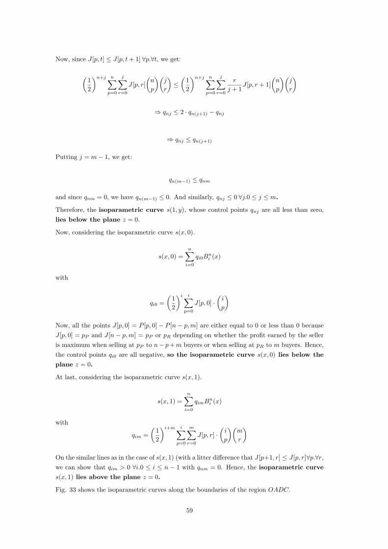
Fig. 33 shows the isoparametric curves along the boundaries of the region OADC.

59

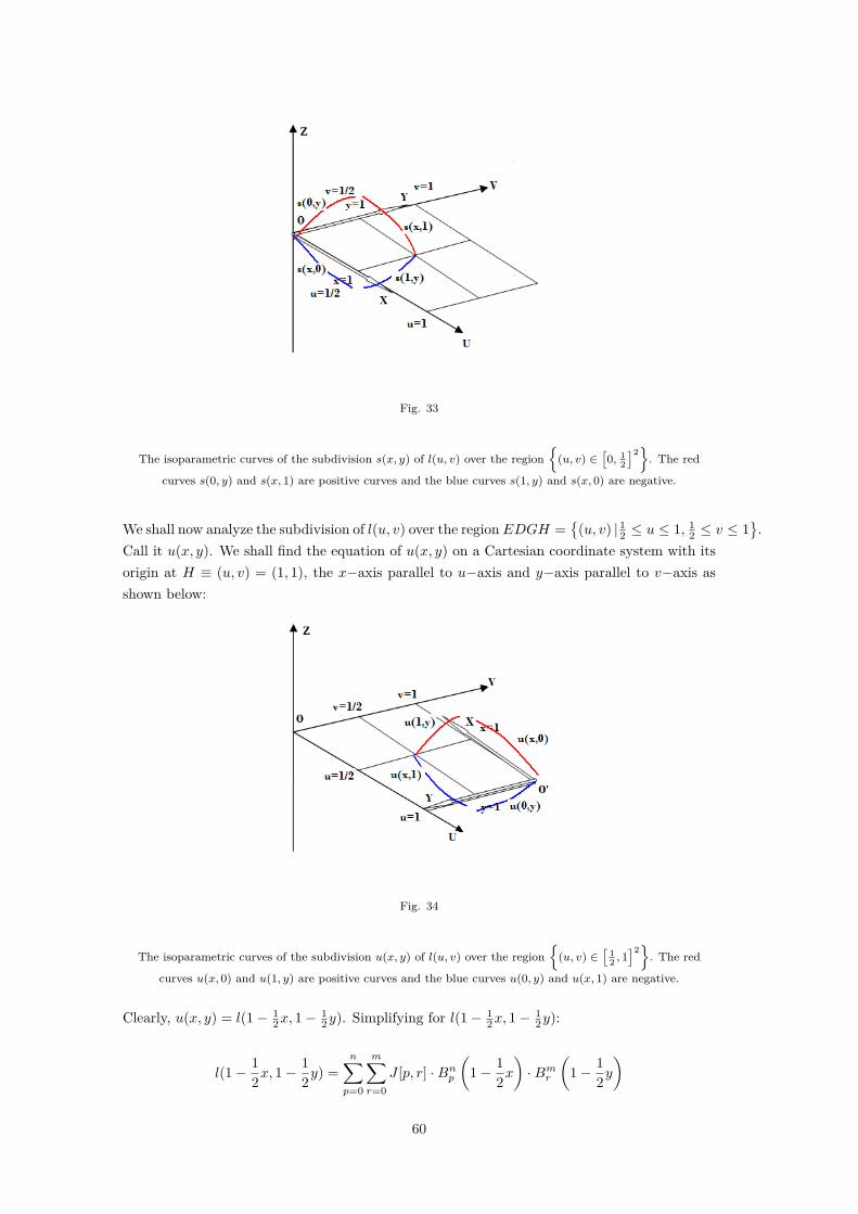
Fig. 33

The isoparametric curves of the subdivision s(x, y) of l(u, v) over the region{

(u, v) ∈[0, 1

2

]2}. The red

curves s(0, y) and s(x, 1) are positive curves and the blue curves s(1, y) and s(x, 0) are negative.

We shall now analyze the subdivision of l(u, v) over the region EDGH ={(u, v) | 12 ≤ u ≤ 1, 1

2 ≤ v ≤ 1}.

Call it u(x, y). We shall find the equation of u(x, y) on a Cartesian coordinate system with itsorigin at H ≡ (u, v) = (1, 1), the x−axis parallel to u−axis and y−axis parallel to v−axis asshown below:

Fig. 34

The isoparametric curves of the subdivision u(x, y) of l(u, v) over the region{

(u, v) ∈[

12 , 1]2}. The red

curves u(x, 0) and u(1, y) are positive curves and the blue curves u(0, y) and u(x, 1) are negative.

Clearly, u(x, y) = l(1− 12x, 1−

12y). Simplifying for l(1− 1

2x, 1−12y):

l(1− 12x, 1− 1

2y) =

n∑p=0

m∑r=0

J [p, r] ·Bnp(

1− 12x

)·Bmr

(1− 1

2y

)

60

=n∑p=0

m∑r=0

J [p, r] ·(n

p

)(1− 1

2x

)p·(

12x

)n−p(m

r

)(1− 1

2y

)r (12y

)m−r

Replacing n− p by p and m− r by r and adjusting the summations, we get:

l(1−12x, 1−1

2y) =

0∑p=n

0∑r=m

J [n−p,m−r]·(

n

n− p

)(1− 1

2x

)n−p·(

12x

)p(m

m− r

)(1− 1

2y

)m−r (12y

)r

As J [p, r] = P [p, r] − P [n − p,m − r] = − (J [n− p,m− r]− J [p, r]) = −J [n − p,m − r], wehave:

l(1−12x, 1−

12y) = −

0∑p=n

0∑r=m

J[p, r]·(np

)(1−

12x

)n−p·(

12x

)p (mr

)(1−

12y

)m−r ( 12y

)r= −

0∑p=n

0∑r=m

J[p, r]Bnp

(12x

)·Bmr

(12y

)

⇒ l(1− 12x, 1− 1

2y) = u(x, y) = −s(x, y)

Now, u(0, y) = −s(0, y) ⇒ u(0, y) lies below the plane z = 0.

u(1, y) = −s(1, y) ⇒ u(1, y) lies above the plane z = 0.

u(x, 0) = −s(x, 0) ⇒ u(x, 0) lies above the plane z = 0.

u(x, 1) = −s(0, y) ⇒ u(x, 1) lies below the plane z = 0.

Fig. 34 shows the isoparametric curves along the boundaries of the region EDGH.

Let us also analyze the isoparametric curves of l(u, v) along the boundaries of the unit squareOBHF (Fig. 30) for the sake of completeness.

l(u, v) =n∑p=0

m∑r=0

J [p, r] ·Bnp (u) ·Bmr (v)

Consider l(0, v):

l(0, v) =n∑p=0

m∑r=0

J [p, r] ·Bnp (0) ·Bmr (v)

⇒ l(0, v) =m∑r=0

J [0, r] ·Bmr (v)

J [0, r] = P [0, r] − P [n,m − r] is either positive or zero because J [0, r] = pR ∀r. So, as thecontrol points of the bezier curve l(0, v) are all non-negative, the curve l(0, v) lies above theplane z = 0.

Consider l(1, v):

61

l(1, v) =n∑p=0

m∑r=0

J [p, r] ·Bnp (1) ·Bmr (v)

⇒ l(1, v) =m∑r=0

J [n, r] ·Bmr (v)

J [n, r] = P [n, r]−P [0,m− r] is either negative or zero because J [0,m− r] = pR ∀r and J [n, r]may be pP or pR. So, as the control points of the bezier curve l(1, v) are all non-positive, thecurve l(0, v) lies below the plane z = 0.

Consider l(u, 0):

l(u, 0) =n∑p=0

m∑r=0

J [p, r] ·Bnp (u) ·Bmr (0)

⇒ l(u, 0) =n∑p=0

J [p, 0] ·Bnp (u)

J [p, 0] = P [p, 0]−P [n− p,m] is either negative or zero because J [p, 0] = pP ∀p and J [n− p,m]may be pP or pR. So, as the control points of the bezier curve l(u, 0) are all non-positive, thecurve l(u, 0) lies below the plane z = 0.

Consider l(u, 1):

l(u, 1) =n∑p=0

m∑r=0

J [p, r] ·Bnp (u) ·Bmr (1)

⇒ l(u, 1) =n∑p=0

J [p,m] ·Bnp (u)

J [p,m] = P [p,m]−P [n− p, 0] is either positive or zero because J [n− p, 0] = pP ∀p and J [p,m]may be pP or pR. So, as the control points of the bezier curve l(u, 1) are all non-negative, thecurve l(u, 1) lies above the plane z = 0.

Fig. 35 shows the isoparametric curves of l(u, v) along the boundaries of the region OBHF .

62

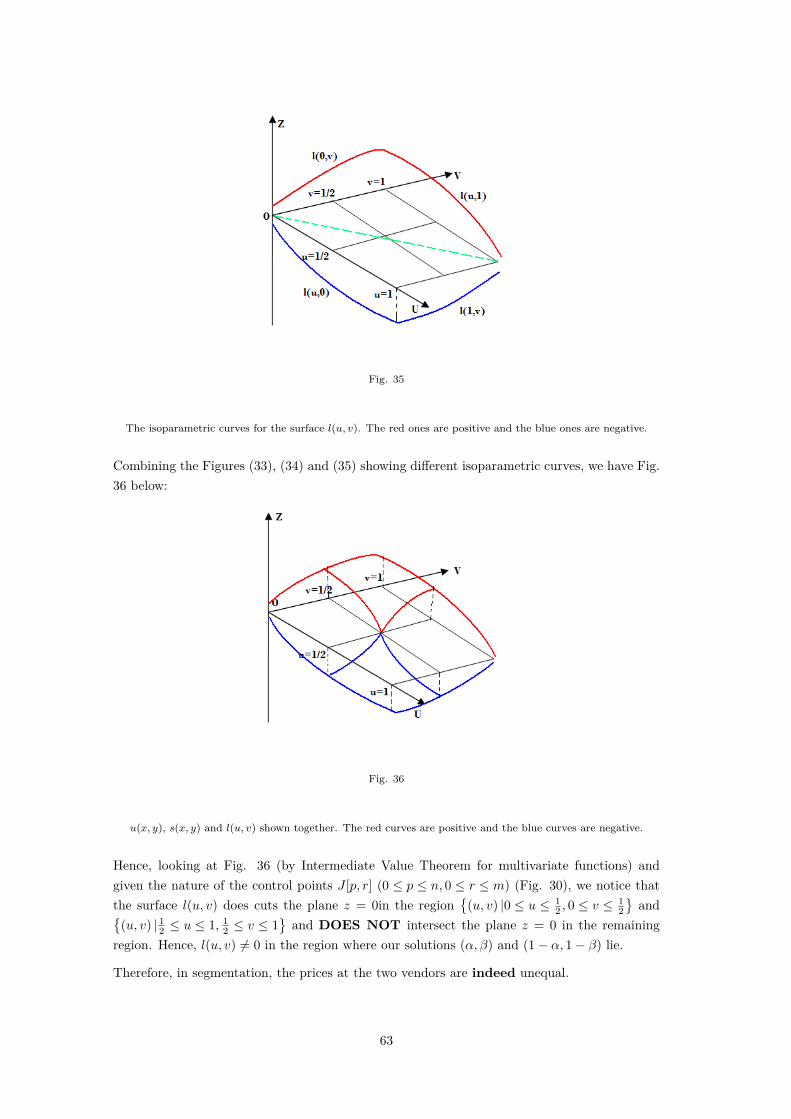
Fig. 35

The isoparametric curves for the surface l(u, v). The red ones are positive and the blue ones are negative.

Combining the Figures (33), (34) and (35) showing different isoparametric curves, we have Fig.36 below:

Fig. 36

u(x, y), s(x, y) and l(u, v) shown together. The red curves are positive and the blue curves are negative.

Hence, looking at Fig. 36 (by Intermediate Value Theorem for multivariate functions) andgiven the nature of the control points J [p, r] (0 ≤ p ≤ n, 0 ≤ r ≤ m) (Fig. 30), we notice thatthe surface l(u, v) does cuts the plane z = 0in the region

{(u, v) |0 ≤ u ≤ 1

2 , 0 ≤ v ≤12}and{

(u, v) | 12 ≤ u ≤ 1, 12 ≤ v ≤ 1

}and DOES NOT intersect the plane z = 0 in the remaining

region. Hence, l(u, v) 6= 0 in the region where our solutions (α, β) and (1− α, 1− β) lie.

Therefore, in segmentation, the prices at the two vendors are indeed unequal.

63

Part V

Conclusion and Future WorkIn the above analysis of the game, we computed the pure strategy and mixed strategy Nashequilibria. We have shown that in a randomized strategy equilibrium, all the poor buyers choosebetween the two vendors with the same probability and all the rich buyers choose between thetwo vendors with the same probability (other than the one of poor’s) leading to the conclusionthat there are situations under which segmentation in the market can take place even if there aretwo identical vendors. We also proved the inequality of prices at the two vendors in equilibrium.

Cooperative analysis of this game can be undertaken as a part of future research to study theeffect of coalition formation between the buyers.

64

Part VI

References[1] “Game Theory - Analysis of Conflict” by Roger B. Myerson, Harvard University Presspaperback edition, 1997.

[2] Lecture Notes for the course CADG 2006 (http://www.cse.iitb.ac.in/~sohoni/336/main.ps)by M. Sohoni, Computer Science and Engineering, IIT Bombay.

[3] War and Peace, Nobel Prize lecture. December 8, 2005 by Robert J. Aumann, Center forthe Study of Rationality, and Department of Mathematics, The Hebrew University, Jerusalem,Israel.

[4] Introduction to Game Theory by Martin J. Osborne ISBN-13: 978-0-19-568158-1.

65

Btp Report

Documents

Transcript of Btp Report