BSP-Based Support Vector Regression Machine Parallel Framework

BSP-Based Support Vector Regression Machine Parallel Framework

Hong Zhang

School of Computer Engineering and Science

Shanghai University

149 YanChang Road, ZhaBei District

Shanghai, 200072, P.R. China

E-mail: [email protected]

Yongmei Lei

School of Computer Engineering and Science

Shanghai University,

149 YanChang Road, ZhaBei District

Shanghai, 200072, P.R. China

E-mail: [email protected]

In this paper, we investigate the distributed parallel Support Vector Machine training strategy, and then propose a

BSP-Based Support Vector Regression Machine Parallel Framework which can implement the most of distributed

Support Vector Regression Machine algorithms. The major difference in these algorithms is the network topology

among distributed nodes. Therefore, we adopt the Bulk Synchronous Parallel model to solve the strongly connected

graph problem in exchanging support vectors among distributed nodes. In addition, we introduce the dynamic

algorithms which can change the strongly connected graph among SVR distributed nodes in every BSP’s super-step.

The performance of this framework has been analyzed and evaluated with KDD99 data and four DPSVR

algorithms on the high-performance computer. The results prove that the framework can implement the most of

distributed SVR algorithms and keep the performance of original algorithms.

Keywords: parallel computing; bulk synchronous parallel; support vector regression machine (SVR); regression

prediction.

1. Introduction

In modern learning theory, time efficiency and the

accuracy of results are always the goals to pursue. With

the coming of big data era, traditional support vector

regression machine (SVR) [1] training algorithms take a

lot of time. In order to improve learning speed of SVR

under large-scale data and keep global optimal,

distributed parallel learning technology is an inevitable

way. So the distributed parallel support vector

regression machine (DPSVR) training algorithms

appear. However, since the DPSVR training problem is

a stochastic problem, there is no perfect algorithm to

solve the general problem.

Support vector machine (SVM)[2] is supervised

learning model that analyzes data and recognizes

patterns. Owing to its good quality to solve the problem

of high dimensional model construction with limited

samples and its capability of generalization, SVM is

widely used for classification and regression analysis. In

1996, SVR was proposed by Vapnik, and it has

important theoretical significance and application value

for function fitting problem. But there exists a

constrained quadratic programming problem to be

solved, the drawback of SVM is the complexity of

implementation.

A lot of speedup implementations of the quadratic

programming algorithm for SVM have been proposed

International Journal of Networked and Distributed Computing, Vol. 1, No. 3 (August 2013), 134-143

Published by Atlantis Press Copyright: the authors

134

willieb

Typewritten Text

Received 16 April 2013

willieb

Typewritten Text

Accepted 15 June 2013

willieb

Typewritten Text

willieb

Typewritten Text

Hong Zhang, Yongmei Lei

such as chunking [3] and Sequential Minimal

Optimization [4].

Another effective solution is parallel training

strategy. Parallel training strategy is more suitable for

SVM, by splitting the problems into smaller sub-

problems. There are two kinds of parallel training

strategy: task parallel and data parallel. Task parallel

mainly splits the matrix in quadratic programming

algorithm to parallel process [5]. The data parallel splits

the training set and it is easy to be used in distributed

applications. Therefore, the data parallel SVM also has

been known as distributed parallel support vector

machine (DPSVM).

Some DPSVM algorithms [6][7] which find SVs in

local processing nodes and gather them in a master data

processing node to form a new SVM training dataset to

produce training model. But their solutions are local

optimum, not global optimum. Caragea[8] improved

this algorithm by allowing the master data processing

node to send SVs back to the distributed data processing

nodes and do it repeatedly to achieve the global

optimum. Then, for the sake of accelerating DPSVM,

Graf [9] had come up with an algorithm that

implemented distributed nodes into cascade top–down

network topology, namely, cascade SVM. This

algorithm increases the number of SVM sub-problem to

be processed, but it reduces the average processing scale

of these problems. In general, the cascade SVM is the

fastest DPSVM algorithm. However, some researchers

[10][11] improved this structure to obtain more

satisfying results in specified cases. And the basic idea

of these improved algorithms is to change the network

topology among distributed nodes. In 2008, Yumao Lu

[12] proved that the global optimal of DPSVM can be

achieved iteratively if and only if its network topology

is strongly connected graph.

Since there is no perfect DPSVR algorithm to solve

the general problem, a parallel framework which can

implement the most of DPSVR algorithms is a good

solution to speed up to solve the general SVR problem.

Therefore, in order to find the parallel framework, a

parallel model should be introduced to solve the

problem of communication along the network topology.

Malewicz[13], in Google, proposed a framework for

processing large graphs that is expressive and easy to

program. The framework is called Pregel which is

inspired by Bulk Synchronous Parallel (BSP) model

[14].

By integrating SVR theory and DPSVM evolution

process with the BSP model, we propose a BSP-Based

Support Vector Regression Machine Parallel

Framework. It can implement the most of DPSVM

algorithms.

This paper is organized as follows. Support vector

regression problem is introduced and formulated in Sect

2. In sect 3, there is a brief introduction of Bulk

Synchronous Parallel model. Then we would present

BSP-Based Support Vector Regression Machine

Parallel Framework in Sect 4, followed by our

experiments and results in Sect 5. We discuss some

issues and conclude this paper in Sect 6.

2. Brief View of Support Vector Regression

The main characteristic of SVR is that instead of

minimizing the observed training error, SVR attempts to

minimize the generalized error bound to achieve

generalized performance [15]. The generalized error

bound is combination of the training error and a

regularization term which controls the complexity of the

hypothesis space.

Compared to the statistical regression procedures,

SVR shows strong robustness in the regression problem

by introducing insensitive loss function. The model

produced by SVR depends on a subset of the training

data, because the cost function for building the model

ignores any training data close to the model prediction

within a threshold ε.

2.1. Linear Support Vector Regression

Consider the problem [16][17] of approximating the

following data set:

1 1{(x , y ),..., (x , y )},x ,n

l lD R y R (1)

With a linear function:

(x) , , ,bf w x b w X R (2)

where <,> denotes the dot product and binary group (x , y )i i represents a training sample of the training set D,

and parameter l represents the size of the training set. In

ε-SVR, the goal is to search for an optimal linear fitting

function f(x) that estimates the values of output

variables with deviations less than or equal to ε from the

actual training data. The optimal regression function [18]

is:

Minimize 2

1

*(ξ ξ1

|| w | )|2

l

i

i iC

(3)


135


Subject to

i i

*

i i

*

i i

y , b ξ

, b y ξ

ξ ,ξ 0

w x

w x

i

i (4)

Where ξ i and *ξ i are relaxation variables introduced to

satisfy constraints on the function. Therefore, SVR fits a

function to the given data by not only minimizing the

training error but also by penalizing complex fitting

functions. This penalty is acceptable only if the fitting

error is larger than ε. The ε-insensitivity loss

function ,i iy f x x

is defined by:

ε

y x ,x max 0, y x , x εi i i if f (5)

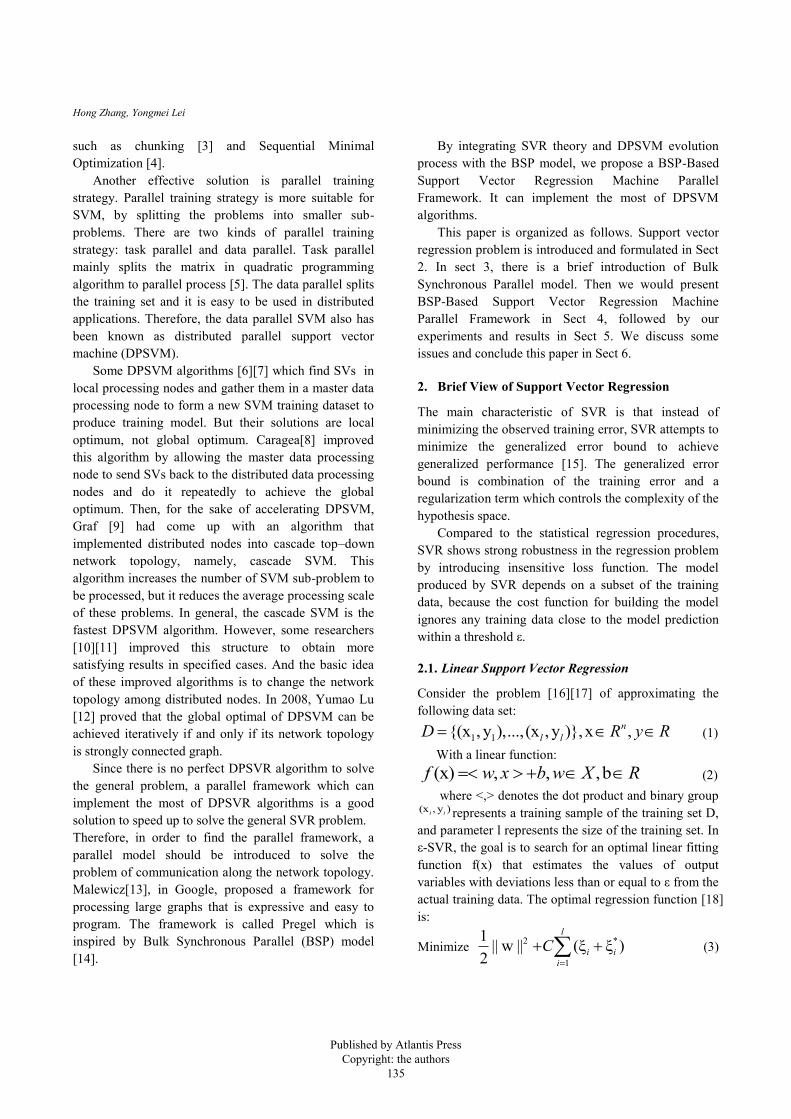
As presented in Figure 1, the ε-insensitive loss

function can be visualized as a tube equivalent to the

approximation accuracy that surrounds the training data.

The primal function, namely the optimization problem

given by (3) can be solved more easily in its dual

formulation. The key idea is to construct a Lagrange

function from the objective function and constraints by

introducing a dual set of variables. The new dual

objective function can be formulated as follows:

2

1 1

* *

1 1

*

* *

ξ ξ α ε ξ , b1

( ) ( )2

( ) ( )α ε ξ , b

l l

i

i i

l l

i i i i

i

i i i i

i i

i

i

y w x

y w x

L w C

i

i

(6)

Where L is the Lagrange function and i ,*

i , αi and *αi are non-negative Lagrange multipliers. The partial

derivatives of L with respect to the primal variables (w,

b, ξ i , *ξ i ) vanish at the optimum (actually a saddle

point).

l

*

i i

i 1

Lα α 0

b

(7)

l

*

i i i

i 1

Lw α α x 0

w

(8)

i i

i

LC α η 0

ξ

(9)

* *

i i*

i

LC α η 0

ξ

(10)

Substituting (7), (8), (9) and (10) into (6) generates

the following dual optimization problem:

* *

, 1

* *

1 1

1α α α α x x

2

ε α α y α α

l

i i j j i

i

j

l l

i i i i i

j

i i

Maximize

(11)

Subject to

*

1

*,

α α 0

α α 0,

l

i i

i

i

i C

(12)

After solving the dual problem the optimal decision

can be obtained:

*

1

x α α <x , x> bi i i

i

l

f

(13)

Equation (13) is called the support vector expansion.

Computation of b is done by exploiting the KKT

conditions which state that the product between dual

variables and constraints vanishes at the optimal

solution. This lead to:

i i i i

* *

i i i i

α ξ ε y w, x b 0

α ξ ε y w, x b 0

(14)

And

i i

* *

i i

C α ξ 0

C α ξ 0

(15)

Based on (14) and (15), it can be concluded that only

samples (x , y )i i with *

i C lie outside the ε-

insensitive tube. Furthermore, * 0i i shows that a set

of dual variables * i i are never both nonzero. And for

the *

(0,C)i , *

0i , the second term in (14) must

vanish.

Based on (11), the Lagrange multipliers may be

nonzero if ,i iy f x x which indicates that all Lagrange

multipliers inside the ε-tube vanish. On the other hand,

the second term in formulas (14) is nonzero for ,i iy f x x , which implies that the multipliers have to

be zero to satisfy the KKT conditions. This

demonstrates that the SVR uses only a fraction of the

training data to express the original data and

approximate the target function [15].

Fig. 1. Soft margin loss setting for a linear SVR[18].


136


2.2. Nonlinear Support Vector Regression

As for the nonlinear regression problem, they are more

common and useful in practical application. The key

and fundamental idea to solve this problem is to use the

kernel function. Kernel functions can project the data

into a higher dimensional feature space to improve the

capability of the linear machine to represent the

nonlinear relationship that exists in the original input

space. Furthermore using the kernel function also can

get rid of the complexity of dot product operation in

high dimensional space. This leads to the following

optimization problem to determine the flattest function

in the feature space:

* *

, 1

* *

1 1

1α α α α K(x x

2

ε α α

)

y α α

i j

i

l

i i j j i j

l l

i i i

i

i i

Maximize

(16)

Subject to

*

1

*,

α α 0

α α 0,

l

i i

i

i

i C

(17)

The corresponding optimal decision function of (9)

is shown as follows:

*

1

x α α K(x , x) bl

i i i

i

f

(18)

A function can be used as a kernel function if and

only if it satisfies the Mercer’s condition.

From the above, we can see that SVR problem is a

constrained quadratic programming problem. It is rather

slow and computationally expensive for quadratic

programming to converge to a solution. Therefore, we

should introduce a parallel model to accelerate the

computational procedure and the model should have the

ability to process the network topology among

distributed parallel nodes.

3. Bulk Synchronous Parallel Model

The BSP [19] model provides a simple framework for

the design and programming of all kinds of general

purpose parallel systems. Algorithms designed for such

a model should be relatively easy to analyze and result

in predictable, portable and efficient programs.

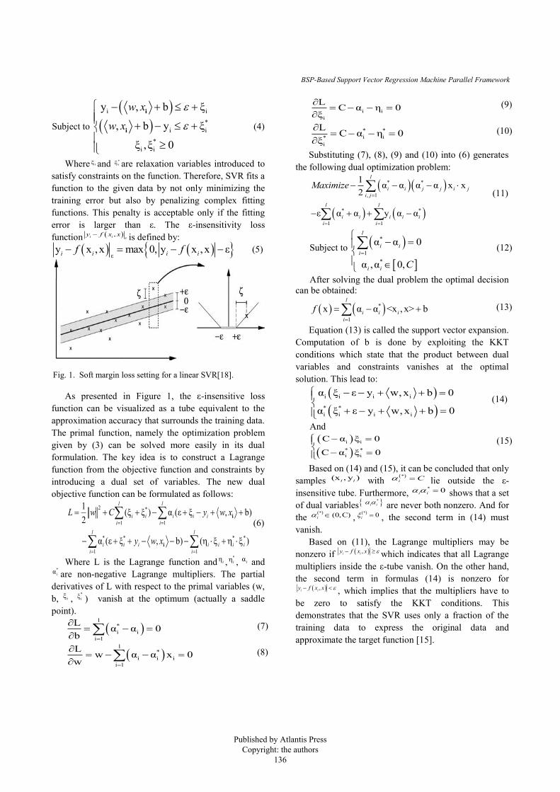
A BSP computation proceeds in a series of global super-

steps. A super-step consists of three components, as the

figure shows below:

Concurrent computation: several computations take

place on every participating processor. Each

process only uses values stored in the local memory

of the processor. The computations are independent

in the sense that they occur asynchronously of all

the others.

Communication: The processes exchange data

between themselves. This exchange takes the form

of one-sided Put and Get calls, rather than two-

sided Send and Receive calls.

Barrier synchronization: When a process reaches

the barrier, it waits until all other processes have

finished their communication actions.

The concept and idea of super-step in BSP model

inspired us to take the BSP model into DPSVR.

Because of the DPSVR algorithms using feedbacks

to get global optimal, the communication network

topology can be regarded as strong connected graph. So

the BSP model solves the communication problem in

our framework.

4. BSP-Based Support Vector Regression

Machine Framework

4.1. Framework Description

For the purpose of improving learning speed of SVR

problem and overcoming the training difficulties under

large-scale data, distributed parallel learning technology

is an inevitable way. Simultaneously, because of the

DPSVR algorithms which get global optimal using

feedback and iteration, the communication network

topology can be regarded as a strong connected graph.

Therefore, the BSP model is adopted to solve the

communication problem in DPSVR algorithms.

Consequently, we proposed this framework on the basis

of the SVR algorithm, strong connected graph theory

and the BSP model.

The framework could solve most of DPSVR

algorithms, such as cascade SVR algorithm [8][9][10],

gather SVR algorithm [7]. What’s more, it can solve

Fig. 2. Three components of a super-step[20].


137


other DPSVR algorithms as long as the communication

network topology of the algorithm among distributed

nodes is a strong connected graph. The same as BSP

model, our framework consists of a lot of super-steps.

The concept of super-step in our framework is a unit

of parallel iteration. It also contains three steps. First

step, we use parallel training algorithm which based on

data space decomposition to train SVR sub-problems in

several nodes. Then, we pass the result set of SVs to

some other nodes along the edge of strong connected

graph. At last, we compare the difference between the

SVs generated by super-step n and the SVs from super-

step n-1 with a given value in each node. If the

difference is less than the given value, we would judge

that the node votes for halt. The framework adopts the

master-slave model to collect all of the halt information

to judge whether the whole task is finished or needs a

next super step.

The framework takes the training samples and graph

of network topology among the nodes as the input. In

order to achieve initial training samples load balancing,

we use rolling iterative strategy to divide the whole of

training sample set.

If the graph input is a dynamic change, the user need

implement the dynamic graph-change API. The

dynamic graph need contain a loop to cyculate in order

to guarantee the graph being a strong connected graph.

And the number of super-step in a loop period is used in

deciding whether the task is finished or not. It will be

shown with cascade SVM algorithm in Sect 5. The

static strong connected graph can be seen as a special

dynamic strong connected graph which the loop period

of super-step is 1. The advantage of dynamic strong

connected graph is that it can reduce the number of

processing nodes. Take the example of 3-tier cascade

SVR algorithm, it would take 15 nodes to process in

static strong connected graph, but it only needs 8 nodes

in dynamic version. It has been shown as follows:

4.2. Strategy of Implementation Framework

The BSP-Based Support Vector Regression Machine

Parallel Framework is made up of master node and

slave nodes. Each node is responsible for training the

corresponding sub-task, passing the SVs derived from

the sub-task and judging local task whether halt or not.

And the regression model will be generated by the

master node when master node collects the whole

judging results and decides to terminate the task. The

processing steps of framework are defined as follows:

Step1: Masker node gets the input data including

training samples and the graph of network topology

among the distributed nodes (static or dynamic);

Step2: Each node reads corresponding training

samples;

Step3: Each node reads the graph of network

topology and dynamic changes the strong

connected graph if it is necessary;

Step4: Each node generates the corresponding

training sub-data;

Step5: Each node trains sub-data and obtains final

decision function and support vectors;

Step6: Each node delivers the SVs along the edge

of strong connected graph;

Step7: Each node gathers the SVs from other nodes.

Step8: Each node eliminates repetition SVs, and the

remaining SVs would be added to next super-step

training sub-data;

Step9: Each node judges whether halt or not

according to difference between the SVs generated

at this time and last time.

Step10: Masker node gathers the halt information

from all nodes and decides if the task is finished or

not. If not, go to Step 3 to do next super step;

Step11: Master node would generate regression

model if the task is finished.

The step 1 and step 2 are the initialization of the

framework. The step 3 to step 9 constitute a super step,

each super-step is a parallel computing process. After

each super-step, the parallel framework will judge

whether the result of this super-step is the global

optimum.

And, compared to the time complexity of computing

sub-task 3 3( / )O N M , the time complexity of

communication among distributed nodes O(NM) is

much more less. N is the size of training set, M is the

number of computing nodes. In general, N is far more

than M. So the framework could keep the performance

of original algorithms when training set is in large scale.

The flow diagram of framework is showed below:

0 2 3 4 5 6 71

0 2 4 6

0 4

0

0 2 3 4 5 6 71

8 9 10 11

12 13

14

Dynamic cascade DPSVR

topology graph

Static cascade DPSVR topology graph

Fig. 3. Static cascade DPSVR and Dynamic cascade DPSVR

topology graph.


138


5. Experiment and Analysis

5.1. Experiments Description

The framework is implemented by C, C++ and MPI

parallel library, and we employ four kinds of cross-

compiler including g++, gcc, mpic++, mpicc [21][22].

The experiment data is from KDD99 [23], KDD99 are

the safety audit datasets announced by Columbia

University IDS laboratory led by professor Stolfo,

which is from 1998 MITLL IDS datasets, and only

include network traffic data. Since the KDD99 original

dataset is too large (734MB) [23], considering the

convenience of the experiment, [7][22] has selected part

of datasets as experiment data from the original KDD99.

Here, we use one datasets of them to experiment. The

dataset details show in Table 1.

Table 1. Experimental Dataset.

Dataset

Name

The Total

Number of

Records

The Number

of Normal

Records

The Number

of Abnormal

Records

The Size

of Dataset

Dataset 190578 69865 120713 19.4 MB

Experiment is implemented by two steps:

Step1: Parallel training datasets Dataset in different

number of nodes and different algorithms, then we

can obtain corresponding regression model;

Step2: Test each above-mentioned regression

model by using testing dataset Dataset and give the

corresponding testing result of each model;

The graphs of network topology in algorithm used in

the experiment are ring graph, full connected graph,

gather graph, cascade graph. Taking 8 nodes as example,

the graphs shows below:

Dynamic change the strong

connected graph


connected graph……


connected graph

Computing sub-task

Computing sub-task

……Computing

sub-task

Obtain support vectors

Obtain support vectors

……Obtain support

vectors

Gather support vectors

Gather support

vectors……

Gather support

vectors

SVs SVs SVsSVs SVs SVs SVsSVs

Eliminate repetition SVs

Eliminate repetition SVs

……Eliminate

repetition SVs

Judge halt Judge halt …… Judge halt

Master node P0 decide if the task is finished or not?

Generate regression model

Yes


connected graph




connected graph

nonono no

The training samples and strong connected graph as

input

The average distribution of sample set


connected graph




connected graph

Master node P0 decide if the task is finished or not?

Generate regression model

Yes

nonono no

…… …… …… ……

Super Step 1 ~ N-1

Super Step N

Super Step N+1

Node P0

generating sub-data

Node P1

generating sub-data ……Node Pn-1

generating sub-data

Fig. 4. BSP-Based Support Vector Regression Machine

Framework.

2

6

4

5

3

7

0

1

Fig. 6. Ring topology graph.

1 2 3 4

5670

Fig. 5. Ring topology graph.


139


Moreover, we present the expansibility and the

dynamic changeability of our parallel framework in

gather topology graph and cascade topology graph. It

provides the graph-change API for changing the graph

dynamic with the number of super-step. The graph has

been expressed in programming language in the form of

adjacency matrix. The value equals 1 in adjacency

matrix position (i, j) means that node i would transmit

SVs to node j in this super-step. Take the example of 8

nodes cascade topology graph. In super-step 1, the

adjacency matrix of cascade topology graph is:

1

1 0 0 0 0 0 0 0

1 0 0 0 0 0 0 0

0 0 1 0 0 0 0 0

0 0 1 0 0 0 0 0

0 0 0 0 1 0 0 0

0 0 0 0 1 0 0 0

0 0 0 0 0 0 1 0

0 0 0 0 0 0 1 0

C

And, in the super-step 2, the adjacency matrix of cascade topology graph has changed to:

2

1 0 0 0 0 0 0 0

0 0 0 0 0 0 0 0

1 0 0 0 0 0 0 0

0 0 0 0 0 0 0 0

0 0 0 0 1 0 0 0

0 0 0 0 0 0 0 0

0 0 0 0 1 0 0 0

0 0 0 0 0 0 0 0

C

Then, in the super-step 3, the adjacency matrix of

cascade topology graph has changed to:

3

1 0 0 0 0 0 0 0

0 0 0 0 0 0 0 0

0 0 0 0 0 0 0 0

0 0 0 0 0 0 0 0

0 0 0 0 1 0 0 0

0 0 0 0 0 0 0 0

0 0 0 0 0 0 0 0

0 0 0 0 0 0 0 0

C

In the super-step 4, the adjacency matrix of cascade

topology graph has changed to:

4

1 1 1 1 1 1 1 1

0 0 0 0 0 0 0 0

0 0 0 0 0 0 0 0

0 0 0 0 0 0 0 0

0 0 0 0 0 0 0 0

0 0 0 0 0 0 0 0

0 0 0 0 0 0 0 0

0 0 0 0 0 0 0 0

C

After reached and finished 4C and it will go back to 1C , it will loop this procedure.

5.2. Experiments Results and Analysis

In our study, we get the training time in the learning

process through BSP-Based Support Vector Regression

Machine Framework. According to the training dataset

shown in Table 1, Table 2 gives final training results

and the corresponding testing results of Step 2. In the

experiments we choose Radial Basis Function kernel

and set the parameters as follows. We set Penalty

parameter C=1, kernel parameter σ=0.1 and Tolerance

parameter ε=0.1[6]. In order to evaluate the

performance of tests quantitatively evaluation indicators

are defined as follows:

Detection Precision (DT): the correct number of

detected records / the total number of records;

False Positive (FP): the number of records which

are normal records being mistaken abnormal

records / the number of normal records;

0 2 3 4 5 6 7

0

1

Fig. 7. Gather topology graph (dynamic).

0 2 3 4 5 6 71

0 2 4 6

0 4

0

Fig. 8. Cascade topology graph (dynamic).


140


False Negative (FN): the number of records which

are abnormal records being mistaken normal

records / the number of abnormal records.

Super-step N: the number of super-step has been

executed during the training problem.

The normal records are these normal TCP

connection records. And the abnormal records are those

network attack records.

Results of the experiments demonstrate that the

BSP-Based Support Vector Regression Machine

Parallel Framework can implement most of DPSVR

algorithms and have the ability to dynamically change

the network topology. It is also proved that the

framework has strong extensibility, and it is easy to

program and test for new DPSVR algorithms.

Table 2. Performances of training set Dataset s:/seconds

Nodes Algorithm Type Training Time /s DT FP FN Super-Step N

1 Serial 667.75 0.9833 0.0017 0.0253 1

4 Ring graph 650.17 0.9850 0.0019 0.0256 4

4 Full connected graph 328.88 0.9833 0.0017 0.0253 2

4 Gather graph 350.15 0.9833 0.0017 0.0253 3

4 Cascade graph 351.74 0.9833 0.0017 0.0245 4

8 Ring graph 942.07 0.9825 0.0018 0.0266 8


8 Gather graph 269.38 0.9833 0.0017 0.0253 3

8 Cascade graph 268.55 0.9827 0.0017 0.0263 5

12 Ring graph 1172.24 0.9823 0.0017 0.0269 12


12 Gather graph 258.47 0.9835 0.0018 0.0250 3

12 Cascade graph 196.04 0.9828 0.0018 0.0260 5

Table 2 shows that the result is global optimum

when the input graph is strong connect graph. Because

ring graph algorithm need to travel the whole graph, it

performs less well in figure 9. And other algorithms

have reduced the training time as the number of nodes

increasing. The cost time of one super-step depends on

Fig. 10. Training time per super-step of 4 algorithms.

Fig. 9. Training time of 4 algorithms..


141


the maximum time from all nodes. Therefore, in full

connected graph SVR algorithm and gather graph SVR

algorithm the SVs from all nodes will be added to one

node at a super-step, the scale of training data in one

node may be much bigger than the initial data.

Consequently, the full connected graph SVR algorithm

and gather graph SVR algorithm perform worse than

cascade SVR algorithm in our dataset. And, the figure

10 about training time per super-step also demonstrates

it. With the number of nodes increasing, the training

time does not decrease notably. It is also because of the

training data from other nodes is equal or more than the

initial local training data. This indicated that the parallel

number of computing nodes is not the more the better.

The number may be related to the ratio between the size

of training set and the size of result SVs, the way that

training set distributed, and so on.

6. Discussion and Conclusions

Above all, we have proposed a BSP-Based Support

Vector Regression Machine Parallel Framework that is

able to solve large-scale SVR training problems and it is

free to choose appropriate DPSVR algorithm. Only if

the graph input is a strong connect graph, the framework

will output the global optimum. What’s more, we have

implemented the API of graph-change to dynamic

change the graph. It would be used to load balancing

and other expansion.

The results of experiment prove that our framework

could adapt to most of DPSVR algorithms. Meanwhile,

it could get the high precision in the regression and keep

a good speedup of original algorithm.

Furthermore, from the experiment result, we can

comprehend that the time efficiency about DPSVR

algorithm is related to the number of super-step and the

maximum time in every super-step. The number of

super-step depends on the strategy to terminate the task

and the condition to halt in each node. The problem of

maximum time in every super-step is about load

balancing.

Even though there is no perfectly DPSVR algorithm

to solve the general SVR problem, we have the

possibility to use this parallel framework to dynamically

solve the general problem.

Since the DPSVR algorithm’s time efficiency is in

relation to the maximum time cost in every super-step

and the number of super-step, our further research is

going to investigate the load balancing between the

super steps. For example, the framework running

cascade algorithm will choose appropriate nodes and

quantity to merge. In addition, we will explore the

relationship between the appropriate number of nodes

and the ratio between the size of training set and the size

of result SVs.

Acknowledgements

This work is supported in part by Innovation Research

program of Shanghai Municipal Education Commission

under Grant 12ZZ094, and High-tech R&D Program of

China under Grant 2009AA012201, and Shanghai

Academic Leading Discipline Project J50103.

References

1. V.Vapnik, S.Golowich, A Smola. Support Vector Method

For Function Approximate on Regression Estimation and

signal Processing Advances in Neural Information

Processing Systems. 1997.

2. V.Vapnik. The Nature of Statistical Learning Theory [M].

New York: Springer-Verlag, 1999.

3. Osuna E, Freund R, Girosi F. “An improved training

algorithm for support vector machine,” Proceedings of

IEEE Neural Networks for Signal Processing, Amelia

Island, 1997.

4. Plat, J., “Sequential Minimal Optimisation: a fast

algorithm for training support vector machines”, Techn.

Rep.MSR-TR-98-14, Microsoft Research, 1998.

5. G. Zanghirati and L. Zanni, “A parallel solver for large

quadratic programs in training support vector machines,”

Parallel Comput., vol. 29, pp. 535–551, 2003.

6. N. Syed, H. Liu, and K. Sung, “Incremental learning with

support vector machines,” in Proc. 5th ACM SIGKDD

Int. Conf. Knowl. Disc. Data Mining, San Diego, CA,

1999.

7. Lei Yong-mei, Yan Yu, Chen Shao-jun. Parallel Training

Strategy Based on Support Vector Regression Machine,

Dependable Computing, 2009 15th IEEE Pacific Rim

International Symposium on Dependable Computing,

2009, pp.159-164.

8. C. Caragea, D. Caragea, and V. Honavar, “Learning

support vector machine classifiers from distributed data

sources,” in Proc. 20th Nat. Conf. Artif. Intell. Student

Abstract Poster Program, Pittsburgh, PA, 2005, pp.

1602–1603.

9. H. P. Graf, E. Cosatto, L. Bottou, I. Durdanovic, and V.

Vapnik, “Parallel support vector machines: The cascade

SVM,” in Proc. 18th Annu. Conf. Neural Inf. Process.

Systems, Vancouver, BC, Canada, 2004, pp. 521–528.

10. Jing Yang, “An Improved Cascade SVM Training

Algorithm with Crossed Feedbacks,” Computer and

Computational Sciences, vol.2, pp.735-738, 2006


142


11. Zhongwei Li, “A Support Vector Machine training

Algorithm based on Cascade Structure”, Innovative

Computing, Information and Control, vol.3, pp.440-443,

2006.

12. Yumao Lu, Vwani Roychowdhury, Lieven

Vandenberghe, “Distributed Parallel Support Vector

Machines in Strongly Connected Networks,” IEEE

Transactions on Neural Networks, vol. 19, no.7 pp.1167-

1178, July 2008

13. G. Malewicz, M. H. Austern, A. J. Bik, J. C. Dehnert, I.

Horn, N. Leiser, and G. Czajkowski, “Pregel: a system

for large-scale graph processing,” in Proceedings of the

2010 international conference on Management of data,

ser. SIGMOD ’10. New York, NY, USA: ACM, pp.135–

146, 2010.

14. Leslie G. Valiant, “A Bridging Model for Parallel

Computation,” Comm. ACM vol.33, no.8, pp.103-111,

1990

15. D. Basak, S. Pal, D.C. Patranabis “Support vector

regression,” Neural Information Processing—Letters and

Reviews, vol.11, no.10, pp.203–224, 2007

16. Wang Dingcheng, Fang Tingjian, Tang Yi, Ma Yongjun.

Review of Support Vector Machines Regression Theory

and Control [J], Pattern Recognition and Artificial

Intelligence, vol.16, no.2, pp.192-197, 2003.

17. A.F. Al-Anazi, I.D. Gates. Support vector regression for

porosity prediction in a heterogeneous reservoir: A

comparative study[J], Computers & Geosciences,vol.36,

no.12, pp.1494-1503, 2010

18. ALEX J. SMOLA,BERNHARD SCHOELKOPf.A

tutorial on support vector regression[J], Statistics and

Computing, vol.14, no.3, pp.199-222, 2004

19. W.F. McColl Scalability, portability and predictability:

The BSP approach to parallel programming Future

Generation Computer Systems, vol.12, pp. 265–272,

1996

20. http://en.wikipedia.org/wiki/Bulk_synchronous_parallel

21. Zhi-Hui DU, San-Li LI. Parallel programming

technology in high-performance computing- MPI parallel

programming, the first edition. BeiJing: Tsinghua

University Press, ISBN 7-302-04566-6/ TP.2703, August

2001

22. Ronggang Jia, Yongmei Lei, Gaozhao Chen, Xuening

Fan. “Parallel Predicting Algorithm Based on Support

Vector Regression Machine,” Computer and Information

Science (ICIS), 2012 IEEE/ACIS 11th International

Conference on Computer and Information Science (ICIS),

pp.488-493, 2012

23. Zhang Xin-you, Zeng Hua-shen, Jia Lei. Research of

intrusion detection system dataset-KDD CUP99 [J],

Computer Engineering and Design, vol.31, no.22,

pp.4809-4816, 2010

24. http://kdd.ics.uci.edu/databases/kddcup99/kddcup99.html


143

BSP-Based Support Vector Regression Machine Parallel Framework

Documents

Transcript of BSP-Based Support Vector Regression Machine Parallel Framework