Brownian trading excursions and avalanches

Friedrich Hubalek∗ Paul Kruhner† Thorsten Rheinlander‡

January 5, 2017

We study a parsimonious but non-trivial model of the latent limit orderbook where orders get placed with a fixed displacement from a center priceprocess, i.e. some process in-between best bid and best ask, and get executedwhenever this center price reaches their level. This mechanism corresponds tothe fundamental solution of the stochastic heat equation with multiplicativenoise for the relative order volume distribution. We classify various typesof trades, and introduce the trading excursion process which is a Poissonpoint process. This allows to derive the Laplace transforms of the timesto various trading events under the corresponding intensity measure. As amain application, we study the distribution of order avalanches, i.e. a seriesof order executions not interrupted by more than an ε-time interval, whichmoreover generalizes recent results about Parisian options.

1 Introduction

The main object of interest in this study is to develop a parsimonious model of the limitorder book (LOB) for financial assets, where price level and number of orders away fromthe best bid/ask prices are recorded. We refer to [CJP15] for an overview of marketmicrostructure trading.

Quite a few articles on the LOB, starting amongst others with Kruk [Kru03], areinvestigating the limiting behavior of some discretely modeled dynamics. Cont and deLarrard [CdL13] model the dynamics of best bid and ask quotes as two interacting

∗Financial and Actuarial Mathematics, Vienna University of Technology, Wiedner Haupt-straße 8/ 105-1, 1040 Vienna, Austria. phone +43-1-58801-10511 fax +43-1-58801-9-105199(fhubalek@fam.tuwien.ac.at)

†Financial and Actuarial Mathematics, Vienna University of Technology, Wiedner Haupt-straße 8/ 105-1, 1040 Vienna, Austria. phone +43-1-58801-10552 fax +43-1-58801-9-10552(paulkrue@fam.tuwien.ac.at)

‡Financial and Actuarial Mathematics, Vienna University of Technology, Wiedner Haupt-straße 8/ 105-1, 1040 Vienna, Austria. phone +43-1-58801-10550 fax +43-1-58801-9-10550(rheinlan@fam.tuwien.ac.at)

1

arX

iv:1

701.

0099

3v1

[q-

fin.

MF]

4 J

an 2

017

queues. Their structural model combines high frequency price dynamics with the or-der flow, and a Markovian jump-diffusion process in the positive orthant is reached asscaling limit. Horst et al. [BHQ14] derive a functional limit theorem where the limits ofthe standing buy and sell volume densities are described by two linear stochastic par-tial differential equations, which are coupled with a two-dimensional reflected Brownianmotion that is the limit of the best bid and ask price processes, whereas Abergel andJedidi [AJ13] consider the volume of the LOB at different distances to the best ask priceand determine a diffusion limit for the mid price. Delattre et al. [DRR13] study theefficient price which is a price market practitioners could agree upon and its statisticalestimation. The placing of orders is captured by Osterrieder [Ost06] in a marked pointprocess model, so that the order book is modeled by several measure valued processes.

Our study is quite different to the aforementioned works. For the point of focus, weconsider a latent order book model, see [TLD+11], which contains the orders of low-frequency traders, whereas high frequency orders which get typically cancelled after avery short time span are not recorded. As we are in particular interested how limitorders get intrinsically executed, we do not allow for any other mechanism besides thatthe center price, which we model as a Brownian motion, hits the level where the limitorders are placed. Here orders get issued relative to the actual center price according tosome universal aggregated volume density function.

Expanding formally the relative order volume distribution via Ito’s formula, it resultsthat this volume distribution solves a stochastic heat equation with multiplicative noise,which will be studied in a subsequent paper [HKR17b]. Here we are interested in thefundamental solution, which corresponds to order placement according to a Dirac mea-sure on some level µ away from the best bid or ask price. This leads to an approachable,but nonetheless highly non-trivial model of limit order executions. We do not make anyclaims that our model is realistic, but it should be understood as a parsimonious modelwhich can later be extended in various directions, like more sophisticated models for theorder arrival process as well as for the center price.

In this context, we discuss in detail and classify various types of trading times whichcan be characterized via doubly reflected Brownian motion. There are two basic execu-tion mechanisms for the ask side of the book (which one can then subdivide further):a Type I trade occurs whenever the price maximum increases, whereas a Type II tradeis triggered after a downfall by more than the displacement followed by an equal surgeof the center price. We then study excursions to the next trading time. The tradingexcursion process is a Poisson point process, for which the intensity measure is known.This allows us to calculate the Laplace transforms under the intensity measure of thetimes to various types of trades in terms of hypberbolic functions.

A major application of these results is the study of order execution avalanches, i.e. aseries of order executions not interrupted by more than an ε-time interval. One has toallow for a small time window where orders do not get executed due to the fact thatBrownian motion has no point of increase. Here we drew some inspiration from the paperStapleton and Christensen [SC06] about avalanches which is in the spirit of the theoryof self-organized criticality. We derive the Laplace transform of the general avalanchelength of order execution in our model, which improves over several known results in the

2

context of Parisian options before, in particular by Dassios and Wu [DW15] as well asGauthier [Gau02]. A similar result for simple avalanches (not containing Type II trades)has been proved by Dudok de Wit [DdW13] by a different method in a limit order bookframework.

The structure of the paper is as follows: In the next section, we introduce our latentlimit order book model, in particular the order placement and execution mechanisms.Section 3 contains the classification of various types of trading times, followed by ananalysis of the order book with Dirac-type placement. In Section 5 the central idea oftrading excursions is introduced, which leads in Section 6 to the hyperbolic functiontable regarding Laplace transforms of the times to various trading events. As our mainapplication, we derive in Section 7 the Laplace transform of the order avalanche length.

2 A Brownian motion model for the limit order book

As in [RY99, Sec.XII.2, p.480] we shall work with the canonical version W of Brownianmotion on the Wiener space (W,F , P ). This means W is the space of continuousfunctions w : R+ → R with w(0) = 0, equipped with the locally uniform topology, Pis the Wiener measure, F is the Borel σ-field of W completed with respect to P , andWt(w) = w(t) for t ≥ 0 and w ∈W.

We denote by Lat : a ∈ R, t ∈ R+ a bicontinuous modification of the family of localtimes of W , see [RY99, Thm.VI.1.7, p.225].

We assume that orders arrive with density one in every infinitesimal time interval dt,model the center price process W as a Brownian motion, and denote by F = (Ft)t≥0 itsaugmented filtration. This ‘center price’ is just thought to lie in between best bid andask, see below for the precise order execution mechanism at best bid/ask.

2.1 Absolutely continuous order placement

Let V (t, x) denote the order volume at time t ≥ 0 and level x ∈ R. The placement ofnew limit orders is governed by some integrable function g : R \ 0 → R+. An intuitivedescription of the dynamics is as follows:

• During an infinitesimal time interval dt, it is assumed that new limit orders arecreated at every level Wt + x with volume density g(x)dx,

• limit orders at level x are executed once the center price hits the correspondinglevel, i.e. when Wt = x,

• there will be no order withdrawal.

For a rigorous definition let us denote by

σ(t, x) := sups ∈ [0, t] : Ws = x or s = 0 (1)

3

the last exit time of W from level x before time t. Consider now a time t ≥ 0 and alevel x ∈ R. At time σ(t, x) all orders at level x are executed. The volume V (t, x) ismade up from new orders placed during the time interval (σ(t, x), t] and thus we define

V (t, x) :=

∫ t

σ(t,x)g(x−Ws) ds. (2)

Note that order execution is included in (2) since the integral gets void once W reachesthe level x, capturing the aforementioned execution mechanism. In particular V (t,Wt) =0 for all t ≥ 0.

We distinguish the bid order book and the ask order book processes, which we defineas

V (t, x) := V (t, x)Ix≤Wt , V (t, x) := V (t, x)Ix≥Wt . (3)

Obviously1 we have V (t, x) = V (t, x) + V (t, x).

Definition 1. The best ask process α is given by

α(t) := infx ∈ R : V (t, x) > 0, t > 0 (4)

and the best bid process β is given by

β(t) := supx ∈ R : V (t, x) > 0, t > 0 (5)

Remark 2. It is shown in Hubalek, Kruhner and Rheinlander [HKR17b] that the relativevolume random field v (t, x) := V (t, x+Wt) is a weak solution (in an appropriate sense)of the SPDE

dv(t, x) =

(1

2∂2xv(t, x) + g(x)

)dt+ ∂xv(t, x)dWt, (6)

v(0, x) = 0, v(t, 0) = 0, ∀(t, x) ∈ R+ × R, (7)

and V can be expressed in terms of Brownian local time Ly at the level y as

V (t, x) =

∫R

(Lx−yt − Lx−yσ(t,x)

)g(y)dy, (8)

which follows from (2) by the occupation times formula, cf. [RY99, Corollary VI.1.6].

2.2 General order placement

In view of (8), we propose for a finite Borel measure G with G(0) = 0 the order bookprocess

V (t, x) =

∫R

(Lx−yt − Lx−yσ(t,x)

)G(dy). (9)

1We have V (t, x) ≥ 0 and V (t, x) ≥ 0. Some authors, for example [CST10, Sec.1.1, p.550] distinguishthe bid and ask side of the order book by attaching a negative sign to the bid volume.

4

The decomposition into bid and ask (3) and the definitions for best bid and ask (4)and (5) apply unchanged also to the model with general order placement.

Of particular importance for the analysis is the case when order placements are notabsolutely continuous, but occur only at a fixed distance µ > 0 from the center. Thiscorresponds to choosing

G(dx) = δ−µ(dx) + δµ(dx), (10)

with δ±µ denoting the Dirac distribution at ±µ, and leads to

V (t, x) = Lx+µt − Lx+µ

σ(t,x), V (t, x) = Lx−µt − Lx−µσ(t,x), (11)

where Lxt denotes the Brownian local time at level x.These definitions can be motivated by the analogous notions for the discrete order

book model from [HKR17a], which can be studied by elementary counting of singleorders of size one.

While this basic model is a gross simplification, it nevertheless gives some insight aboutthe classification of trading times, and leads to new mathematical results regarding orderavalanches which have been studied before in the context of Parisian options, see [DW15].Moreover, (11) can be considered as fundamental solution or Green’s function for theSPDE (6) with general order placement intensity g.

3 Trading times – definition and classification

In this section we start with a pathwise analysis of trading times on the Wiener space.For this we consider a fixed w ∈W that admits a continuous local time function L, i.e.L : [0,∞) × R → R+ such that

∫ t0 1w(s)∈Ads =

∫A L

xt dx for any Borel set A ∈ B(R),

t ≥ 0.

Remark 3. To emphasize the pathwise nature of the results in this section we shouldwrite Lxt (w) instead of Lxt and similarily V (t, x, w), V (t, x, w) etc., but for better read-ability we omit the w in the notation.

We define in complete analogy to Equation (11), but now for the single path w,

V (t, x) := Lx+µt − Lx+µ

σ(t,x), V (t, x) := Lx−µt − Lx−µσ(t,x), (12)

α(t) := infx > w(t) : V (t, x) > 0 and β(t) := supx < w(t) : V (t, x) > 0 for t > 0,x ∈ R.

The trading times are exactly the times when the path w hits the best ask α, resp.the best bid β.

Definition 4. We define the set of ask trading times Θ and the set of bid trading timesΘ by

Θ := t ≥ 0 : w(t) = α(t), Θ := t ≥ 0 : w(t) = β(t). (13)

Remark 5. In the following we shall focus on the ask side and simply write Θ for Θ.The corresponding definitions and results for the bid side are completely analogous.

5

To classify trading times let us introduce the last and next trading time.

Definition 6. The last trading time before t is

Υ(t) := sups ∈ [0, t) : s ∈ Θ or s = 0, (14)

the next trading time after t is

Ξ(t) := infs ∈ (t,∞) : s ∈ Θ or s =∞. (15)

We start classifying different trades into those trades where the best ask increases(Type I) and those where the best ask decreases (Type II). By convention we considerthe first trade to be of Type II.

Definition 7. The set of Type I trades is defined by

ΘI := t ∈ Θ : α(Υ(t)) ≤ α(t),Υ(t) 6= 0 (16)

the set of Type II trades is

ΘII := t ∈ Θ : α(Υ(t)) > α(t) or Υ(t) = 0.

Schematic illustrations for a Type I resp. Type II trade are given in Fig. 2 resp. inFig. 5.

For a finer classification, we distinguish the cases where trades accumulate (a) beforeand after t, (b) before but not after t, (c) after but not before t, and (d) isolated trades.Thus a priory we have eight types.

Definition 8.

ΘIa := t ∈ ΘI : Υ(t) = t = Ξ(t),ΘIb := t ∈ ΘI : Υ(t) = t < Ξ(t),ΘIc := t ∈ ΘI : Υ(t) < t = Ξ(t),ΘId := t ∈ ΘI : Υ(t) < t < Ξ(t),

ΘIIa := t ∈ ΘII : Υ(t) = t = Ξ(t),ΘIIb := t ∈ ΘII : Υ(t) = t < Ξ(t),ΘIIc := t ∈ ΘII : Υ(t) < t = Ξ(t) andΘIId := t ∈ ΘII : Υ(t) < t < Ξ(t).

(17)

However, we shall see in Proposition 9 that Type IIa and Type IIb trades do not exist,and, then again in a stochastic setup, in Proposition 20 that the probability for isolatedtrades (i.e. Type Id and Type IId) is zero. The only trades that do occur with positiveprobability are Type Ia, Type Ib, Type Ic, and Type IIc.

A schematic illustration for various types of trades is given in Fig. 1 on page 7.

Proposition 9. Type II trades do not accumulate from the left, i.e., we have ΘIIa = ∅and ΘIIb = ∅ for all w ∈W.

Proof. Let t ∈ ΘII and assume that Υ(t) = t. Then α (Υ(t)) = α (t) and hence t /∈ ΘII.Therefore, t ∈ ΘIIc ∪ΘIId .

6

Remark 10. Note that if w0 = 0, and the order book is initially empty, then the firsttrade will be a Type II trade by definition. Moreover, all Type II trades afterwardshappen at levels below or equal the last trading level, whereas Type I trades happen atlevels higher than the last trade. After the first trade, we have the following successionof trades: at first, there are in every ε-interval infinitely many Type Ia trades, until adownward excursion from α, i.e. an upward excursion of α−W from zero.

W0

W0 + µ

W0 − µ

Ask

Bid

II

Ia

II

Ib

Ia

Ic

Ib

Ia

II

Ib Id

II

Ib

II

Wt

αt

Figure 1: A schematic illustration of different types of trading times

We introduce an alternative representation for the best ask process α. This will beused in the next sections for characterising the time to next trade in a probabilistic way.Denote by

w∗(s, t) := sup w(r) : r ∈ [s, t] , w∗(s, t) := inf w(r) : r ∈ [s, t] (18)

the running maximum respectively minimum of the path w in the interval [s, t].

Definition 11. Let

Γs := inft ≥ s : w(t) = w∗(s, t) + µ, Ψs := inft ≥ s : w(t) = w∗(s, t)− µ (19)

7

and define for any n ≥ 0 the times τ0 := 0 and

τn+1 :=

∞ τn =∞Γτn n even, tn <∞Ψτn otherwise.

(20)

We start with a small observation for the time-points τn, n ∈ N.

Lemma 12. The sequence (τn)n∈N is strictly increasing until reaching ∞ and it has nofinite accumulation point.

Proof. Let n ∈ N such that τn 6= ∞. By continuity of w there is η > 0 such that|w(t)−w(τn)| < µ/2 for any t ∈ [τn, τn + η]. Then, w∗(τn, τn + η)−w∗(τn, τn + η) < µand hence Ψτn ,Γτn > τn + η. Consequently, τn+1 > τn + η.

Now assume by contradiction that τn t for some t ∈ (0,∞). By continuity of w,there is η > 0 such that |w(t)−w(s)| < µ/2 for any s ∈ [t−η, t]. Moreover, there is n ∈ Nsuch that |τn − t| ≤ η and hence we have t > τn+1 > τn + η ≥ t. A contradiction.

We can now identify the behavior of the best ask process α in terms of the times(τn)n≥0.

Proposition 13. We have

α(t) =

w∗(τn, t) + µ; τn ≤ t < τn+1, n even

w∗(τn, t); τn ≤ t < τn+1, n odd.

for any t > 0. Moreover, α is a continuous function of finite variation which is non-increasing on t : ∃n ∈ N : τn ≤ t < τn+1, n even and non-decreasing on the compli-ment.

Proof. Define

γ(t) :=

w∗(τn, t) + µ; τn ≤ t < τn+1, n even

w∗(τn, t); τn ≤ t < τn+1, n odd.

for any t > 0. We first show that γ is continuous. Clearly, γ is cadlag and it is continuousoutside τn : n ≥ 0 by definition. Let n ≥ 1 with τn 6=∞.

Case 1: n is even. By definition we have τn = Ψτn−1 and hence w(τn) + µ =w∗(τn−1, τn).

γ(τn−) = limtτn

γ(t) = limtτn

w∗(τn−1, t) = w∗(τn−1, τn)

= w(τn) + µ = w∗(τn, τn) + µ = γ(τn).

Case 2: n is odd. This is proved analogously like the even case.Thus γ is a continuous function. Next we show that α = γ. Now, let t ∈ (τ0, τ1].

Then, γ(t) = w∗(t0, t) + µ and w(s) : s ∈ [0, t] = [w∗(0, t), w∗(0, t)]. Hence Lut > 0 for

8

Lebesgue almost any u ∈ [w∗(0, t), w∗(0, t)] and Lut = 0 for any u ∈ R\[w∗(0, t), w∗(0, t)].

Consequently,

α(t) = infx > w(t) : V (t, x) > 0 = w∗(0, t) + µ = γ(t).

Now let

I := n ∈ N : ∀t ∈ (τn, τn+1] : α(t) = γ(t).Let n ∈ I ∪ 0 and t ∈ [τn+1, τn+2].

Case 1: n + 1 is even. Then, γ(t) = w∗(τn+1, t) and w(t) ≤ w∗(τn+1, τn+2) + µ bydefinition of γ and τn+2. Consequently,

w∗(τn+1, τn+2) = w∗(τ1, τ2) + µ

and hence

V (t, x) =(V (τn+1, x) + Lx−µt − Lx−µτn+1

)1w∗(τn+1,t)<x ≥ V (τn+1, x)1w∗(τn+1,t)<x.

Lemma 41 yields α(t) = w∗(τn+1, t) = γ(t).Case 2: n+ 1 is odd. This works similar and we get n+ 1 ∈ I.By induction N = I ∪ 0 which yields the claim.

Corollary 14. τ1 is the first (ask) trade and τ2n−1 denotes the n-th Type II trade (inthe ask order book) for any n ∈ N.

In view of this corollary we define, for mathematical convenience, the first trade to beof Type II.

Proof. The first statement is immediate from the definition and the second statementfollow immediately from Proposition 13.

Remark 15. In this section we have not used any specific properties of Brownian mo-tion. In fact, we solely argued from the existence of a continuous occupation densitywhich exists a.s. for many processes.

Let X be any continuous semimartingale such that its quadratic variation is given by[X,X](t) =

∫ t0 c(X(s))ds where c : R→ (0,∞) is a continuous function. [RY99, VI.1.7]

yields that it has local time L which is continuous in time and cadlag in its space variable.[RY99, Corollary VI.1.6] yields that for any Borel set A ∈ B(R) we have∫ t

01X(s)∈Ads =

∫ t

0

1X(s)∈A

c(X(s))d[X,X](s) =

∫A

Lxtc(x)

dx

and, hence, X has occupation density ρtx =Lxtc(x) , x ∈ R, t ≥ 0. In particular, if its local

time posses a continuous version, then so does its occupation density.For more details on occupation densities see [GH80].

Remark 16. Throughout this section we worked with the specific Dirac order placement.However, a close inspection of the arguments reveals that this is not strictly necessaryto obtain the preceeding results. If orders are placed with respect to some measure Ginstead, as in Equation (9), and 0 /∈ supp(G), then defining µ := inf supp(G|B(R+))allows to obtain the same results as presented in this section as long as µ > 0.

9

4 Analysis of the Brownian order book with Dirac orderplacement

4.1 Characterizing trading times via a doubly reflected Brownian motion

We return to our stochastic setup as in Section 2.1. Our aim is now to characterizetrading times via a doubly reflected Brownian motion. The results from the precedingsection hold almost surely by the occupation times formula [RY99, Theorem VI.1.6] and[RY99, Theorem VI.1.7].

Remark 17. Firstly, we observe that (τn)n≥0 from Definition 11 is an increasing se-quence of stopping times.

Up to here we have essentially gathered pathwise properties which do not rely onthe specific structure of the Brownian motion except for the continuous sample pathproperty and the existence of a continuous occupation density. This, however, holds formany other processes as well, cf. [Pro04, Theorem IV.76, Corollary IV.2]. For the restof this section we consider features of trading times which appear to be more specific tothe Brownian motion.

Definition 18. Let µ > 0. A [0, µ]-valued stochastic process X is called a doublyreflected Brownian motion if

f(X(t))−∫ t

0

1

2f ′′(X(s))ds, t ≥ 0

is a martingale for any twice continuously differentiable function f : [0, µ] → R withf ′(0) = 0 = f ′(µ).

Recall that [EK86, Theorems 8.1.1, 4.5.4] yield that such a process exist and [EK86,Theorem 4.4.1] yields that its process law is uniquely determined by its initial distributionPX(0).

Theorem 19. The process α−W is a doubly reflected Brownian motion on the interval[0, µ] with (α−W )(0) = µ. Moreover, we have Θ = t : (α−W )(t) = 0.

Clearly, W − β is another doubly reflected Brownian motion on the interval [0, µ] andΘ = t : (W − β)(t) = 0.

Proof. Let f : [0, µ] → R be a twice continuously differentiable function with f ′(0) =0 = f ′(µ) and define R := W − α. Let

I :=

n ∈ N :E

[f(R(τn + 1))− 1

2

∫ τn+1

τnf ′′(R(s))ds

∣∣∣Fη] = f(R(η))−∫ ητn

12f′′(R(s))ds

for any stopping time η ∈ [τn, τn+1]

10

Let n ∈ N be even and define X(t) := W (t+τn)−W (τn) and X∗(t) := inft ≥ 0 : X(t).Then X is a Brownian motion which is independent of Fτn and Proposition 13 yieldsthat R(η + τn) = R(τn) − X(η) + X∗(η) for any random time η which is bounded by∆τn := τn+1− τn. Moreover, the law of X∗−X coincides with the law of −|B| for someBrownian motion B, which follows from a well-known result of Levy, see for example[RY99, Thm.VI.2.3, p.240], and hence

f(R(τn) + (X∗ −X)∆τn(t)) +

∫ t∧∆τn

0

1

2f ′′(R(τn) + (X∗ −X)(s))ds, t ≥ 0

is a martingale. Hence, n ∈ I. For odd n ∈ N similar arguments show that n ∈ I andthus I = N. The tower property yields that (R(t)−

∫ t0

12f′′(R(s))ds)t≥0 is a martingale

and hence R is an [0, µ]-valued process with [R](t) = [W ](t) = t and reflecting boundariesand hence a doubly reflected Brownian motion, cf. [EK86, p. 366].

Next we show that there are no isolated trades, i.e. there are no trades of Type Id orType IId.

Corollary 20. We have no isolated trades, i.e., P (ΘId ∪ ΘIId = ∅) = 1. In particular,we have

P (ΘII = ΘIIc) = 1.

Proof. By Theorem 19 we have to show that a doubly reflected Brownian motion on [0, µ]has P -a.s. no isolated zeros. Using the construction in [KS91], Section 2.8.C, we see thatthis is equivalent to show that a standard Brownian motion has P -a.s. no isolated timesin the set 2zµ : z ∈ Z. This is a consequence of [KS91], Theorem 9.6, Chapter 2.

4.2 Stopping times and trading times

So far we have defined trading times pathwise: t ∈ R+ is a trading time for w ∈ W ifw(t) = α(t, w). We say a random time τ is a trading time, if Wτ = α(τ) a.s. Next, wewill give some examples of trading times which are also stopping times and we will showthat a stopping time which is a trading time is not of Type Ib.

Lemma 21. Let τ be a stopping time such that P (τ ∈ Θ) = 1. Then Ξ(τ) = τ P -a.s.In particular, P (τ ∈ ΘIb) = 0.

Proof. Let ε > 0 and define B(t) := W (t + τ) −W (τ), t ≥ 0. Then, B is a standardBrownian motion. Let σε be the time where B attains its maximum on [0, ε]. Then, σεis measurable and B(σε) > 0 P -a.s. Hence τ + σε is a trading time and, consequently,P (Ξ(τ) = τ) = 1.

Corollary 14 together with Remark 17 reveals that the Type II trades can be enu-merated by stopping times. Lemma 21 shows that the Type Ib trades are not stoppingtimes. This leaves the question whether stopping times can be of Type Ia or Type Ic,which is, indeed, the case.

First entry times of high levels are actually Type Ia trades.

11

Example 22. Let x > µ and γx := inft ≥ 0 : w(t) = x. Then we have

P (γx is a Type Ia trade) = 1.

Proof. By Proposition 13 we have α(t) ≤ w∗(0, t) and clearly w(t) ≤ α(t) for anyt ∈ [τ1,∞). Since

τ1 = inft > 0 : w(t) = w∗(0, t)− µwe have w∗(0, τ1) ≤ µ. Hence, we have τ1 ≤ γx. Thus we get

w∗(0, γx) = x = w(γx) ≤ α(γx) ≤ w∗(0, αx).

and hence γx ∈ Θ.Let ε ∈ (0, γx). Then, there is sε ∈ (γx − ε, γx) such that w(sε) = w∗(0, sε) > µ.

Hence, α(sε) = w(sε) and we have sε ∈ Θ. This implies that Υ(γx) = γx. Lemma 21yields that Ξ(γx) = γx P -a.s. Hence, γx ∈ ΘIa P -a.s.

Example 23. There is a stopping time η such that

P (η is a Type Ic trade) = 1.

Proof. For a stopping time η define the new stopping times

γ0(η) := inft ≥ η : (α−W )(t) = 0,γ1(η) := inft ≥ η : (α−W )(t) = µ/2,γ2(η) := inft ≥ η : (α−W )(t) ∈ 0, µ.

Clearly, γj(η) is P -a.s. finite for any finite stopping time η, j = 0, 1, 2. Moreover,

P ((α−W )(γ2(γ1(η))) = 0) = 1/2

by symmetry and the Markov property for any stopping time η. We have

A(η) := γ2(γ1(γ0(η))) : (α−W )(γ2(γ1(γ0(η)))) = 0 ⊆ ΘIc

for any finite stopping time η.Define η0 := τ2 where τ2 is given in Definition 11. Observe that w(τ2) 6= α(τ2).

Define recursively

ηn+1 :=

ηn if α(ηn) = w(ηn),

γ2(γ1(γ0(ηn))) otherwise.

Then, (ηn)n∈N converges P -a.s. in finitely many steps. Denote η∞ := limn→∞ ηn.Clearly, α(η∞) = w(η∞) P -a.s. Moreover, denote η− := ηsupn∈N:ηn 6=η∞. Then,we have γ2(γ1(γ0(η−))) = η∞. Consequently,

P (η∞ ∈ ΘIIc) = 1.

12

5 Trading excursions

5.1 The trading excursion process

Theorem 19 shows that trading times correspond to the zeroes of the Markov processesX and Y defined by

X = α−W, Y = W − β. (21)

This allows to study trading times by using excursion theory. Let us recapitulate brieflythe terminology and notation of excursion theory, for background and more details werefer the reader to [RY99, Ch.XII] and [Blu92].

For w ∈W defineR(w) = inft > 0 : w(t) = 0. (22)

Let U+ denote all nonnegative functions w such that 0 < R(w) < ∞, let δ denote thefunction that is identically zero, and set U+

δ = U+ ∪ δ, and let U+δ denote the trace of

the Borel σ-field on W in U+δ .

First we note that X is a continuous semi-martingale, namely doubly reflected Brow-nian motion on [0, µ]. Thus it admits a local time at zero that satifies the Tanakaformula,

Lt(X) = |Xt| − |X0| −∫ t

0sgn(Xs)dXs, t ≥ 0. (23)

Consider the inverse local time process,

τ s(X) = inft ≥ 0 : Lt(X) ≥ s, s > 0. (24)

Definition 24. The trading excursion process for the ask-side is the process (es, s > 0),i.e. the zero-excursion process for X. The trading excursion process for the bid-side isthe process (es, s > 0) i.e. the zero-excursion process for Y .

This means, that e and e are defined on Ω×R+ and take values in U+δ as follows, see

[RY99, Def.XII.2.1, p.480]:

1. If ∆τ s(X) > 0, then es(w) is the map

r 7→ es(r, w) = I[r≤∆τs(w)]Xτs−(w)+r(w), (25)

2. if ∆τ s(X) = 0, then es(w) = δ.

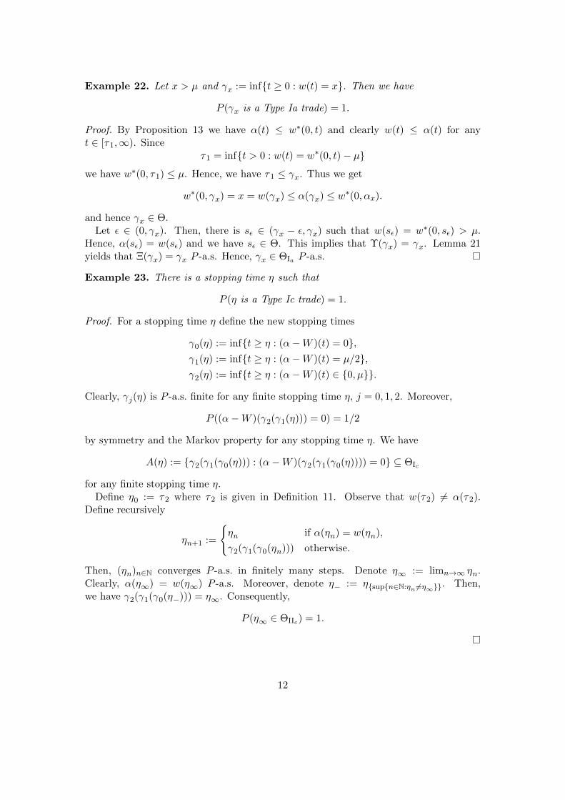
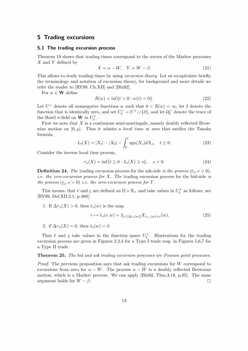
Thus e and e take values in the function space U+δ . Illustrations for the trading

excursion process are given in Figures 2,3,4 for a Type I trade resp. in Figures 5,6,7 fora Type II trade.

Theorem 25. The bid and ask trading excursion processes are Poisson point processes.

Proof. The previous proposition says that ask trading excursions for W correspond toexcursions from zero for α − W . The process α − W is a doubly reflected Brownianmotion, which is a Markov process. We can apply [Blu92, Thm.3.18, p.95]. The sameargument holds for W − β.

13

τs− τs

Figure 2: Ask trade of Type I

Figure 3: Corresponding path of α−W

Figure 4: Corresponding excursion es

14

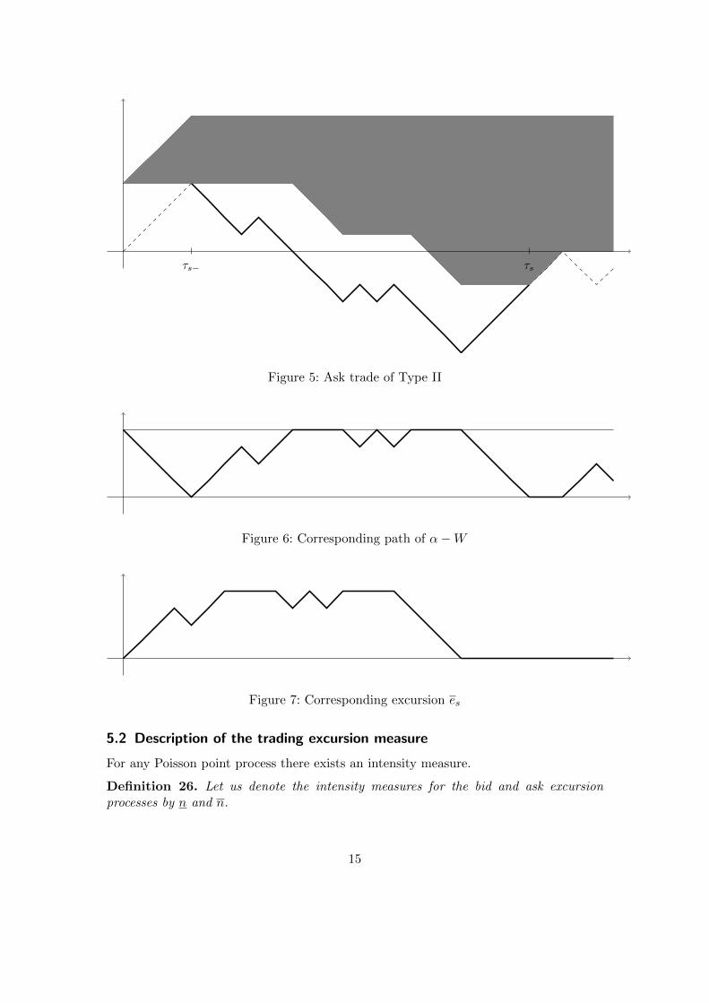
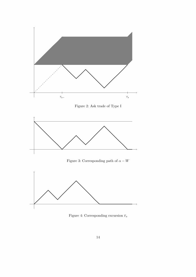
τs− τs

Figure 5: Ask trade of Type II

Figure 6: Corresponding path of α−W

Figure 7: Corresponding excursion es

5.2 Description of the trading excursion measure

For any Poisson point process there exists an intensity measure.

Definition 26. Let us denote the intensity measures for the bid and ask excursionprocesses by n and n.

15

The measures n and n are σ-finite measures on U+δ , and satisfy

n(Γ) =1

tE[NΓ

t ], n(Γ) =1

tE[N

Γt ], t > 0, (26)

whereNΓt =

∑0<s<t

IΓ(es), NΓt =

∑0<s<t

IΓ(es), Γ ∈ U+δ . (27)

Remark 27. In the following we focus on n because n = n.

Let us recall a convenient notation from Williams [Wil91, Sec.5.0, p.49], for the integralof a measurable function F : U+

δ :→ R with respect to the measure n and a set Γ ∈ U+δ ,

n(F ) =

∫F (u)n(du), n(F ; Γ) =

∫ΓF (u)n(du). (28)

For better readability, we shall also write n[F ] and n[F ; Γ] instead of n(F ) and n(F ; Γ)when the expressions for F or Γ are more involved. Furthermore, let us introduce forx > 0 and u ∈ C(R+;R) the hitting time

Tx(u) = inft > 0 : u(t) = x. (29)

We can now give a description of the trading excursion measure that is inspired byWilliams’ description of the Ito measure. Pick three independent processes, namely twoBES3(0) processes ρ and ρ, and a standard Brownian motion b (a BES3(0) processes is aprocess whose law coincides with the law of |B| where B is a three dimensional standardBrownian motion starting in zero.). For all x ∈ (0, µ) we define a process Zx by

Zx =

ρt 0 ≤ t ≤ Tx(ρ),x− ρt−Tx(ρ) Tx(ρ) < t ≤ Tx(ρ) + Tx(ρ),

0 t > Tx(ρ) + Tx(ρ),

(30)

and we define

Zµ =

ρt 0 ≤ t ≤ Tµ(ρ),µ− |bt−Tµ(ρ)| Tµ(ρ) < t ≤ Tµ(ρ) + Tµ(|b|),0 t > Tµ(ρ) + Tµ(|b|).

(31)

Let us introduce length R and height H for excursions u ∈ U+δ by

R(u) = inft > 0 : u(t) = 0, H(u) = supu(t) : 0 ≤ t ≤ R(u), (32)

andRI(u) = R(u)IH(u)<µ, RII(u) = R(u)IH(u)≥µ. (33)

So, RI(u) is the length of a trading excursion that ends with a Type Ic trade, and zerootherwise, whereas RII(u) is the length of a trading excursion that ends with a Type IItrade, and zero otherwise.

16

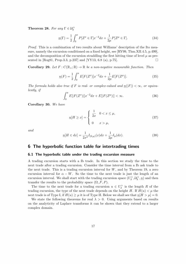
Theorem 28. For any Γ ∈ U+δ

n(Γ) =1

2

∫ µ

0P [Zx ∈ Γ]x−2dx+

1

2µP [Zµ ∈ Γ]. (34)

Proof. This is a combination of two results about Williams’ description of the Ito mea-sure, namely the excursion conditioned on a fixed height, see [RY99, Thm.XII.4.5, p.499],and the decomposition of the excursion straddling the first hitting time of level µ as pre-sented in [Rog81, Prop.3.3, p.237] and [YY13, 6.8 (a), p.75].

Corollary 29. Let F : C(R+;R)→ R be a non-negative measurable function. Then

n(F ) =1

2

∫ µ

0E[F (Zx)]x−2dx+

1

2µE[F (Zµ)]. (35)

The formula holds also true if F is real- or complex-valued and n(|F |) <∞, or equiva-lently, if ∫ µ

0E[|F (Zx)|]x−2dx+ E[|F (Zµ)|] <∞. (36)

Corollary 30. We have

n[H ≥ x] =

1

2x0 < x ≤ µ,

0 x > µ,

(37)

and

n[H ∈ dx] =1

2x2I(0,µ)(x)dx+

1

2µδµ(dx). (38)

6 The hyperbolic function table for intertrading times

6.1 The hyperbolic table under the trading excursion measure

A trading excursion starts with a Ib trade. In this section we study the time to thenext trade after a trading excursion. Consider the time interval from a Ib ask trade tothe next trade. This is a trading excursion interval for W , and by Theorem 19, a zeroexcursion interval for α − W . So the time to the next trade is just the length of anexcursion interval. We shall start with the trading excursion space (U+

δ ,U+δ , n) and then

transfer the results to the probability space (Ω,F , P ).The time to the next trade for a trading excursion u ∈ U+

δ is the length R of thetrading excursion, the type of the next trade depends on the height H. If H(u) < µ thenext trade is of Type I, if H(u) ≥ µ it is of Type II. Below we shall see that n[H > µ] = 0.

We state the following theorems for real λ > 0. Using arguments based on resultson the analyticity of Laplace transforms it can be shown that they extend to a largercomplex domain.

17

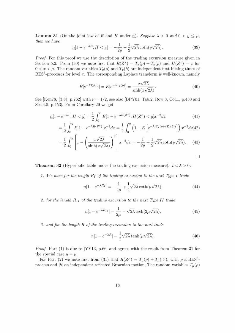
Lemma 31 (On the joint law of R and H under n). Suppose λ > 0 and 0 < y ≤ µ,then we have

n[1− e−λR;H < y] = − 1

2y+

1

2

√2λ coth(y

√2λ). (39)

Proof. For this proof we use the description of the trading excursion measure given inSection 5.2. From (30) we note first that R(Zx) = Tx(ρ) + Tx(ρ) and H(Zx) = x for0 < x < µ. The random variables Tx(ρ) and Tx(ρ) are independent first hitting times ofBES3-processes for level x. The corresponding Laplace transform is well-known, namely

E[e−λTx(ρ)] = E[e−λTx(ρ)] =x√

2λ

sinh(x√

2λ). (40)

See [Ken78, (3.8), p.762] with ν = 1/2, see also [BPY01, Tab.2, Row 3, Col.1, p.450 andSec.4.5, p.453]. From Corollary 29 we get

n[1− e−λT ;H < y] =1

2

∫ µ

0E[1− e−λR(Zx);H(Zx) < y]x−2dx (41)

=1

2

∫ y

0E[1− e−λR(Zx)]x−2dx =

1

2

∫ y

0

(1− E

[e−λ(Tx(ρ)+Tx(ρ))

])x−2dx(42)

=1

2

∫ y

0

1−(

x√

2λ

sinh(x√

2λ)

)2x−2dx = − 1

2y+

1

2

√2λ coth(y

√2λ). (43)

Theorem 32 (Hyperbolic table under the trading excursion measure). Let λ > 0.

1. We have for the length RI of the trading excursion to the next Type I trade

n[1− e−λRI ] = − 1

2µ+

1

2

√2λ coth(µ

√2λ), (44)

2. for the length RII of the trading excursion to the next Type II trade

n[1− e−λRII ] =1

2µ−√

2λ csch(2µ√

2λ), (45)

3. and for the length R of the trading excursion to the next trade

n[1− e−λR] =1

2

√2λ tanh(µ

√2λ). (46)

Proof. Part (1) is due to [YY13, p.66] and agrees with the result from Theorem 31 forthe special case y = µ.

For Part (2) we note first from (31) that R(Zµ) = Tµ(ρ) + Tµ(|b|), with ρ a BES3-process and |b| an independent reflected Brownian motion, The random variables Tµ(ρ)

18

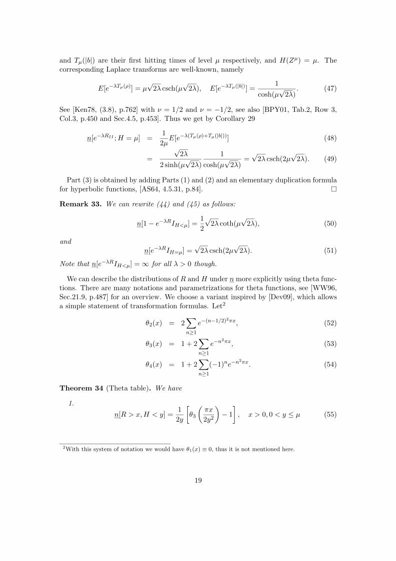
and Tµ(|b|) are their first hitting times of level µ respectively, and H(Zµ) = µ. Thecorresponding Laplace transforms are well-known, namely

E[e−λTµ(ρ)] = µ√

2λ csch(µ√

2λ), E[e−λTµ(|b|)] =1

cosh(µ√

2λ). (47)

See [Ken78, (3.8), p.762] with ν = 1/2 and ν = −1/2, see also [BPY01, Tab.2, Row 3,Col.3, p.450 and Sec.4.5, p.453]. Thus we get by Corollary 29

n[e−λRII ;H = µ] =1

2µE[e−λ(Tµ(ρ)+Tµ(|b|))] (48)

=

√2λ

2 sinh(µ√

2λ)

1

cosh(µ√

2λ)=√

2λ csch(2µ√

2λ). (49)

Part (3) is obtained by adding Parts (1) and (2) and an elementary duplication formulafor hyperbolic functions, [AS64, 4.5.31, p.84].

Remark 33. We can rewrite (44) and (45) as follows:

n[1− e−λRIH<µ] =1

2

√2λ coth(µ

√2λ), (50)

andn[e−λRIH=µ] =

√2λ csch(2µ

√2λ). (51)

Note that n[e−λRIH<µ] =∞ for all λ > 0 though.

We can describe the distributions of R and H under n more explicitly using theta func-tions. There are many notations and parametrizations for theta functions, see [WW96,Sec.21.9, p.487] for an overview. We choose a variant inspired by [Dev09], which allowsa simple statement of transformation formulas. Let2

θ2(x) = 2∑n≥1

e−(n−1/2)2πx, (52)

θ3(x) = 1 + 2∑n≥1

e−n2πx, (53)

θ4(x) = 1 + 2∑n≥1

(−1)ne−n2πx. (54)

Theorem 34 (Theta table). We have

1.

n[R > x,H < y] =1

2y

[θ3

(πx

2y2

)− 1

], x > 0, 0 < y ≤ µ (55)

2With this system of notation we would have θ1(x) ≡ 0, thus it is not mentioned here.

19

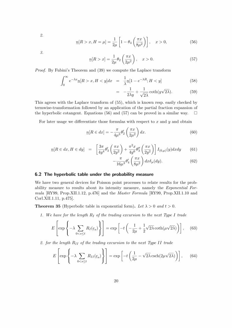
2.

n[R > x,H = µ] =1

2µ

[1− θ4

(πx

8µ2

)], x > 0, (56)

3.

n[R > x] =1

2µθ2

(πx

2µ2

), x > 0. (57)

Proof. By Fubini’s Theorem and (39) we compute the Laplace transform∫ ∞0

e−λxn[R > x,H < y]dx =1

λn[1− e−λR;H < y] (58)

= − 1

2λy+

1√2λ

coth(y√

2λ). (59)

This agrees with the Laplace transform of (55), which is known resp. easily checked bytermwise-transformation followed by an application of the partial fraction expansion ofthe hyperbolic cotangent. Equations (56) and (57) can be proved in a similar way.

For later usage we differentiate those formulas with respect to x and y and obtain

n[R ∈ dx] = − π

4µ3θ′2

(πx

2µ2

)dx. (60)

n[R ∈ dx,H ∈ dy] =

[3π

4y4θ′3

(πx

2y2

)+π2x

4y6θ′′3

(πx

2y2

)]I(0,µ)(y)dxdy (61)

− π

16µ3θ′4

(πx

8µ2

)dxδµ(dy). (62)

6.2 The hyperbolic table under the probability measure

We have two general devices for Poisson point processes to relate results for the prob-ability measure to results about its intensity measure, namely the Exponential For-mula [RY99, Prop.XII.1.12, p.476] and the Master Formula [RY99, Prop.XII.1.10 andCorl.XII.1.11, p.475].

Theorem 35 (Hyperbolic table in exponential form). Let λ > 0 and t > 0.

1. We have for the length RI of the trading excursion to the next Type I trade

E

exp

−λ ∑0<s≤t

RI(es)

= exp

[−t(− 1

2µ+

1

2

√2λ coth(µ

√2λ)

)], (63)

2. for the length RII of the trading excursion to the next Type II trade

E

exp

−λ ∑0<s≤t

RII(es)

= exp

[−t(

1

2µ−√

2λ csch(2µ√

2λ)

)], (64)

20

3. and for the length R of the trading excursion to the next trade

E

exp

−λ ∑0<s≤t

R(es)

= exp

[−t(

1

2

√2λ tanh(µ

√2λ)

)]. (65)

Proof. This follows from the exponential formula with f(s, u) = λRI(u), f(s, u) =λRII(u), f(s, u) = λR(u) and Theorem 32 above.

Remark 36. The sums on the left hand sides are summing over excursions until thelocal time reaches the level t, which corresponds to real time τ t.

Corollary 37 (Hyperbolic table in additive form). Suppose λ > 0 and t > 0.

1. We have for the length RI of the trading excursion to the next Type I trade

E

∑0<s≤t

(1− e−λRI(es)

) = t

[− 1

2µ+

1

2

√2λ coth(µ

√2λ)

]. (66)

2. We have for the time to the next trade T assuming it is Type II

E

∑0<s≤t

(1− e−λRII(es)

) = t

[1

2µ−√

2λ csch(2µ√

2λ)

]. (67)

3. We have for the time to the next trade T

E

∑0<s≤t

(1− e−λR(es)

) = t

[1

2

√2λ tanh(µ

√2λ)

]. (68)

Proof. This follows from the master formula [RY99, XII.1.10] with f(s, u) = 1−e−λRI(u),f(s, u) = 1− e−λRII(u), f(s, u) = 1− e−λR(u) respectively and Theorem 32 above.

7 Laplace transform for the avalanche length

Orders in the LOB get executed via avalanches. In other words, limit orders may ac-cumulate on some levels, and when the price process crosses those values, we will see asudden decrease of the number of orders. We take record if there is no order executionin a time period lasting longer than ε > 0.

Recall from Definitions 4 and 6 that Θ denotes the set of all trading times, Υ(t) (resp.Ξ) denotes the time of last trade before (resp. next trade after) time t.

21

Definition 38. Let

a ∈ Θ, Υ(a) ≤ (a− ε)+, b ∈ Θ, Ξ(b) ≥ b+ ε, (69)

Ξ(t) ≤ t+ ε ∀t ∈ (a, b). (70)

An ε-avalanche is defined as the process Wt : a ≤ t ≤ b. We call a and b start and endof the avalanche. The corresponding ε-avalanche length is b− a.

There is a sequence of stopping times (T an )n≥1 enumerating the start of avalanches,and a sequence of honest times (T en)n≥1 enumerating the end of avalanches (for thecompleted filtration). We are interested into the distribution of the avalanche length forwhich we will rely on the hyperbolic table of the distribution of intertrading times.

Theorem 39. Let T be a stopping time starting an ε-avalanche and Aε be the corre-sponding avalanche length. Then we have the Laplace transform

E[e−λA

ε]

=H(ε)

H(ε) +∫ ε

0 (1− e−λx)h(x)dx. (71)

where

H(ε) =1

2µθ2

(πε

2µ2

), h(x) = − π

4µ3θ′2

(πx

2µ2

). (72)

Proof. Let e denote the trading excursion process for the ask side. We have seen that itis a Poisson point process with intensity measure n. Let R denote the excursion lengthfunctional. Set

Xs =∑

0≤r≤sR(er), s ≥ 0. (73)

By Theorem 35 and Theorem 34 we see that X is a Levy process with Levy measure

νX(dx) = n(dx) = h(x)dx, x > 0. (74)

For ε > 0 we can write X = J + Y with

Ys =∑

0≤r≤s∆XsI∆Xs>ε, Js = Xs − Ys, s ≥ 0. (75)

Then J and Y are two independent Levy processes with Levy measures

νJ(dx) = Ix≤εh(x)dx, νY (dx) = Ix>εh(x)dx, x > 0. (76)

Let S = infs ≥ 0 : ∆Ys > 0. This is the first jump time of a compound Poissonprocess with Levy measure νY and thus exponential with parameter β given by

β = νY (R+) = n[R > ε] = H(ε). (77)

The Levy-Khintchine formula for the cumulant of J says

κ(λ) =

∫ ∞0

(e−λx − 1)νJ(dx). (78)

22

A straight integration gives

κ(λ) = −∫ ε

0(1− e−λx)h(x)dx. (79)

The full avalanche length is A = JS . By independence we obtain the Laplace transform

E[e−λA] =

∫ ∞0

eκ(λ)sβe−βsds =β

β − κ(λ)(80)

and combining this with the results above yields the result.

Remark 40. Let us ignore Type II trades, and assume that orders are only executed as inthe Type I case. Dassios and Wu [DW15] derive the Laplace transform of the avalanchelength Lε in the context of Parisian options. The same formula can be inferred (Dudokde Wit [DdW13]) from the Levy measure of the subordinator consisting of Brownianpassage times. It results that

E[e−λL

ε]

=1

√λεπerf

(√λε)

+ e−λε, (81)

which can be proven in a completely analogous way by choosing h (x) = x−3/2/√

2π, whichis the density of the excursion length T under the Ito measure n, instead of function h. Inthis case the integral in the denominator can be evaluated in terms of the error functionby some elementary computations.

8 Technical remarks, discussions and proofs

8.1 Depth of the order book after the first trade

The next lemma states that the limit order book has an order depth of at least µ afterthe first trade τ1 has happened. Here, we work under the same assumptions as in Section3.

Lemma 41. τ1 is the first trade and for any t ≥ τ1 there is a closed set Kt which is aLebesgue null-set such that

(α(t), α(t) + µ)\Kt ⊆ x ∈ R : V (t, x) > 0 ⊆ (α(t),∞).

Proof. The last inclusion is trivial.For t ∈ [0, τ1] we have V (t, x) = 0 for any x < w∗(0, τ1) +µ and, hence, the first trade

does not take place in [0, τ1). Moreover, we have

w(t) : t ∈ [0, τ1] = [w∗(0, τ1), w∗(0, τ1)] = [w∗(0, τ1), w∗(0, τ1) + µ].

Consequently, L·τ1 has support [w∗(0, τ1), w∗(0, τ1) + µ]. Let

Kτ1 := x ∈ [w∗(0, τ1), w∗(0, τ1)+µ] : Lxτ1 = 0 = x ∈ [w∗(0, τ1), w∗(0, τ1)+µ] : Lx−µτ1 = 0.

23

Then, Kτ1 is closed by continuity of the occupation density and it is a Lebesgue null-set.Clearly, we have

x : V (τ1, x) > 0 = x : Lx−µτ1 > 0 = [w∗(0, τ1), w∗(0, τ1) + µ]\Kτ1 .

The first claim follows.Let T ∈ [τ1,∞] be maximal such that for any t ∈ [τ1, T ) the claim holds. Assume

by contradiction that T < ∞. By continuity of w the claim holds at time T . Again bycontinuity there is δ > 0 such that w∗(T, T + δ) < w∗(T, T + δ). We have

V (t, x) = V (T, x)1σT,t(x)=T + Lx−µt − Lx−µσT,t(x)

where σT,t(x) := infs ∈ [T, t] : w(s) = x or s = T for any x ∈ R, t ∈ [T, T + δ]. Forx > w∗(T, t) we have σT,t(x) = T and hence

V (t, x) = V (T, x) + Lx−µt − Lx−µT

and for x ≤ w∗(T, t) we have V (t, x) = 0. Thus,

x : V (t, x) > 0 = x > w∗(T, t) : V (T, x) > 0 ∪ x ∈ R : Lx−µt − Lx−µT > 0.

This clearly contradicts the maximality of T . Thus T = ∞. The second claim follows.

8.2 Proper trades

The condition for τ to be a trading time of the path w means that the order book is notvoid in any sufficiently small interval (w(τ), w (τ) + ε). This does not necessarily implythat an actual trade takes place at τ . In fact, if the order book is initially empty, then

τ := inf t > 0 : w(t)− infw(s) : s ∈ (0, t) = µ

is the time of the first trade and, if additionally Linfw(s):s∈(0,t)τ = 0 (which happens if

the occupation density is continuous), then V (τ−, α(τ)) = 0, i.e. the limit order bookhas orders only right above the level α(τ). However, this phenomenon is somewhat anartifact of working in continuous time, and for the purposes of the current study it isquite sensible to include such times as well under the label ‘trading times’. In fact,a proper trade takes place at time τ > 0 iff V (τ−, w(τ)) > 0 (and then, as always,V (τ , w(τ)) = 0).

Note, whenever the order volume can be described by a continuous function then thevolume at the best bid and ask will be zero.

Finally, we want to identify the proper trades. First, we need to know that the limitorder book has at least an order depth of µ starting from the first trading time τ1.

Lemma 42. Let η be a random time with η ≥ τ1 where τ1 is defined in Definition 11.Then we have

(α(η), α(η) + µ) ⊆ x ∈ R : V (η, x) > 0 P -a.s.

24

Proof. We have

τ1 = inft > 0 : W∗(0, t) + µ = W ∗(0, t),V (t, x) = Lx−µt − Lx−µσt(x),

x ∈ R : Lx−µt > 0 = (W∗(0, t) + µ,W ∗(0, t) + µ), P -a.s..

Thus, we get

x ∈ R : V (τ1, x) > 0 = W ∗(0, τ1),W ∗(0, τ1) + µ = (α(τ1), α(τ1) + µ) P -a.s.

Thus, for a random time η ≥ τ1 we have

x ∈ R : V (η, x) > 0 ⊇ (α(η), α(η) + µ) P -a.s.

The next proposition identifies the proper trades exactly as the trades of Type Ia andType Ib.

Proposition 43. Let Θ! := t > 0 : V (t−, w(t)) > 0. Then

P (Θ! = ΘIa ∪ΘIb) = 1.

In other words, a proper trade takes place if and only if a trade of Type Ia or Type Ibtakes place.

Proof. Let t ∈ Θ!. Let δ > 0 such that V (t − ε, w(t)) > 0 for any ε ∈ (0, δ). Now letε ∈ (0, δ). Lemma 42 yields that α(t− ε) < w(t). Thus, there is tε ∈ (t− ε, t) such thatα(tε) = w(tε). Hence, we have tε ∈ Θ. Consequently, we have Υ(t) = t which impliest ∈ ΘIa ∪ΘIb .

Now, let t ∈ ΘIa ∪ ΘIb . Proposition 13 yields that there is t0 ∈ [0, t] such thatα(s) = w∗(t0, s) for any s ∈ [t0, t]. Since t /∈ ΘII we have t0 < t. Hence, there ist1 ∈ [t0, t) such that α(t1) + µ > α(t). Lemma 42 yields that V (t1, x) > 0 for anyx ∈ (α(t1), α(t1) + µ) ⊇ [α(t), α(t1) + µ). Consequently, we have V (s, x) > 0 for anys ∈ [t1, t), x ∈ [α(t), α(t1)+µ). This implies that V (t−, w(t)) = V (t−, α(t)) > 0. Hence,t ∈ Θ!.

References

[AJ13] Frederic Abergel and Aymen Jedidi. A mathematical approach to orderbook modeling. International Journal of Theoretical and Applied Finance,16(5):1350025 (40 pages), 2013.

[AS64] Milton Abramowitz and Irene A. Stegun. Handbook of Mathematical Func-tions with Formulas, Graphs, and Mathematical Tables, volume 55 of NationalBureau of Standards Applied Mathematics Series. For sale by the Superin-tendent of Documents, U.S. Government Printing Office, Washington, D.C.,1964.

25

[BHQ14] Christian Bayer, Ulrich Horst, and Jinniao Qiu. A functional limit theoremfor limit order books with state dependent price dynamics. ArXiv e-prints,May 2014.

[Blu92] Robert M. Blumenthal. Excursions of Markov Processes. Birkhauser BostonInc., Boston, MA, 1992.

[BPY01] Philippe Biane, Jim Pitman, and Marc Yor. Probability laws related to theJacobi theta and Riemann zeta functions, and Brownian excursions. Bulletinof the American Mathematical Society, 38(4):435–465, 2001.

[CdL13] Rama Cont and Adrien de Larrard. Price dynamics in a Markovian limitorder market. SIAM Journal on Financial Mathematics, 4(1):1–25, 2013.

[CJP15] Alvaro Cartea, Sebastian Jaimungal, and Jose Penalva. Algorithmic andHigh-Frequency Trading. Cambridge University Press, 2015.

[CST10] Rama Cont, Sasha Stoikov, and Rishi Talreja. A stochastic model for orderbook dynamics. Operations Research, 58(3):549–563, 2010.

[DdW13] Laurent Dudok de Wit. Liquidity Risks Based on the Limit Order Book.Master thesis, TU Wien and EPFL, 2013.

[Dev09] Luc Devroye. On exact simulation algorithms for some distributions relatedto Jacobi theta functions. Statistics & Probability Letters, 79(21):2251–2259,2009.

[DRR13] Sylvain Delattre, Christian Y. Robert, and Mathieu Rosenbaum. Estimatingthe efficient price from the order flow: a Brownian Cox process approach.Stochastic Processes and their Applications, 123(7):2603–2619, 2013.

[DW15] Angelos Dassios and Shanle Wu. Two-side Parisian option with single barrier.Preprint, LSE, Statistics, 2015.

[EK86] Stewart N. Ethier and Thomas G. Kurtz. Markov Processes. John Wiley &Sons, Inc., New York, 1986. Characterization and Convergence.

[Gau02] Laurent Gauthier. Options Reelles et Options Exotiques, une Approche Prob-abiliste. These pour le doctorat, Universite Pantheon-Sorbonne, Paris I,November 2002.

[GH80] Donald Geman and Joseph Horowitz. Occupation densities. The Annals ofProbability, 8(1):1–67, 1980.

[HKR17a] Friedrich Hubalek, Paul Kruhner, and Thorsten Rheinlander. The discreteLOB draft. Work in progress, TU Wien, 2017.

[HKR17b] Friedrich Hubalek, Paul Kruhner, and Thorsten Rheinlander. The SPDE-LOB draft. Work in progress, TU Wien, 2017.

26

[Ken78] John Kent. Some probabilistic properties of Bessel functions. The Annals ofProbability, 6(5):760–770, 1978.

[Kru03] Lukasz Kruk. Functional limit theorems for a simple auction. Mathematicsof Operations Research, 28(4):716–751, 2003.

[KS91] Ioannis Karatzas and Steven E. Shreve. Brownian Motion and StochasticCalculus. Springer-Verlag, New York, second edition, 1991.

[Ost06] Jorg Osterrieder. Arbitrage, Market Microstructure and the Limit OrderBook. PhD thesis, ETH Zurich, 2006.

[Pro04] Philip E. Protter. Stochastic Integration and Differential Equations. Springer-Verlag, Berlin, second edition, 2004.

[Rog81] L. C. G. Rogers. Williams’ characterisation of the Brownian excursion law:proof and applications. In Seminar on Probability, XV (Univ. Strasbourg,Strasbourg, 1979/1980), volume 850 of Lecture Notes in Math., pages 227–250. Springer, Berlin-New York, 1981.

[RY99] Daniel Revuz and Marc Yor. Continuous martingales and Brownian motion.Springer-Verlag, Berlin, third edition, 1999.

[SC06] Matthew Stapleton and Kim Christensen. One-dimensional directed sand-pile models and the area under a Brownian curve. Journal of Physics. A.Mathematical and General, 39(29):9107–9126, 2006.

[TLD+11] B. Toth, Y. Lemperiere, C. Derembleand, J. De Lataillade, J. Kockelkoren,and J.-P. Bouchaud. Anomalous price impact and the critical nature of liq-uidity in financial markets. Phys. Rev. X, 1(2):021006, 2011.

[Wil91] David Williams. Probability with Martingales. Cambridge University Press,Cambridge, 1991.

[WW96] Edmund T. Whittaker and George N. Watson. A Course of Modern Analysis.Cambridge University Press, Cambridge, 1996. Reprint of the fourth (1927)edition.

[YY13] Ju-Yi Yen and Marc Yor. Local Times and Excursion Theory for BrownianMotion, volume 2088 of Lecture Notes in Mathematics. Springer, 2013. Atale of Wiener and Ito measures.

27