Brownian Bridge Vectorial Simulation

J. Beleza Sousa, M. L. Esquıvel, R. M. Gaspar

February 28, 2012

Abstract

The iterative simulation of the Brownian bridge is well known. Inthis paper we present a vectorial simulation alternative. The vecto-rial alternative is based on Gaussian processes for machine learningregression and is suitable for interpreted programming languages im-plementations.

We extend the vectorial simulation to other Gaussian processes,namely, sequences of Brownian bridges, path dependent geometricBrownian motion and path dependent Ornstein-Ulenbeck mean re-version process.

1 Introduction

Interpreted programming languages like Sage, Octave, Mathematica andMatlab are important frameworks in nowadays research and development.

In these programming languages it is crucial to use vectorial algorithmsinstead of iterative ones in order to achieve the execution speeds of compiledlanguages. This is because vectorial operations are typically supported bybuilt-in functions which are implemented by optimized machine code.

The iterative simulation of the Brownian bridge is well known [3][1]. Inthis paper we present a vectorial simulation alternative. The vectorial alter-native is based on Gaussian processes for machine learning regression and issuitable for interpreted programming languages implementations.

We extend the vectorial simulation to other Gaussian processes, namely,sequences of Brownian bridges, path dependent geometric Brownian motionand path dependent Ornstein-Ulenbeck mean reversion process.

1

We illustrate the flexibility of the vectorial simulation by creating a 2DWiener process representation of a Norbert Wiener photograph.

2 Brownian bridge iterative simulation

A Brownian bridge is a standard Brownian motion W conditioned to W (1) =0. The Brownian bridge condition W (1) = 0 can be generalized to other timeinstants greater than zero and to other values besides zero.

The standard Brownian motion W , defined in R+0 , is also called a Wiener

process [2] and has the following properties:

1. W (0) = 0;

2. W has independent increments, i.e. if r < s ≤ t < u then W (u)−W (t)and W (s)−W (r) are independent random variables;

3. For s < t the random variable W (t)−W (s) has the Gaussian distribu-tion N (0,

√t− s);

4. W has continuous trajectories.

In addition, the Wiener process is a Gaussian process with mean functionm(t) and covariance function cov(s, t):

m(t) = 0, (1)

cov(s, t) = min(s, t). (2)

In order to illustrate the iterative simulation of a Brownian bridge tra-jectory B, consider that at some step we have 0 < u < s < t < 1, B(u) = α,B(t) = β and we want to simulate the value B(s) [3]. Given the Wiener pro-cess properties, the random vector [B(u)B(s)B(t)]T is Gaussian with meanvector and covariance matrix: B(u)

B(s)B(t)

∼ N 0

00

, u u uu s su s t

(3)

Therefore the conditional distribution B(s)|B(u), B(t) is given by:

2

B(s)|B(u), B(t) ∼ N(

(t− s)α + (s− u)β

t− u,(s− u)(t− s)

t− u

)(4)

Thus, the value B(s) is simulated by:

B(s) =(t− s)α + (s− u)β

t− u+

√(s− u)(t− s)

t− uZ, (5)

where Z ∼ N (0, 1) is an increment independent of all Z values previouslyused in the simulation.

Finally, the iterative simulation of a Brownian bridge trajectory consistsof starting with u = 0, t = 1, B(0) = 0, B(1) = 0 and iteratively filling atrajectory sample at time s (between u and t) with Equation 5, then movingone of the end points to the simulated sample and repeating the process untilall samples trajectory are filled.

Figure 1 shows a sequence of 500 simulated independent GaussianN (0, 1)increments (white noise), and the corresponding simulated Wiener processand Brownian bridge trajectories (sampled uniformly 500 times between zeroand one). The Brownian bridge trajectory was simulated by the iterativeprocedure above.

3 Gaussian processes for machine learning

The goal of Gaussian processes for machine learning regression is to find thenon linear unknown mapping y = f(x), from data (X,y), using Gaussiandistributions over functions [4]:

GP ∼ N (m(x), cov(x1,x2)). (6)

The pair (X,y) is the training set. The matrix X collects a set of nvectors x where the value y = f(x) was observed. The corresponding yvalues are collected in vector y.

The set of vectors x? where the values y? = f(x?) were not observed, iscollected in matrix X?. The matrix X? is the test set.

The regression function is the mean function of the process defined by allthe trajectories of the process of Equation 6 that passes through the trainingset. The regression confidence is the corresponding covariance function.

3

0.2 0.4 0.6 0.8 1.0

-4-3-2-1

123

HaL

0.2 0.4 0.6 0.8 1.0

0.2

0.4

0.6

0.8

HbL

0.2 0.4 0.6 0.8 1.0

0.2

0.4

0.6

0.8HcL

Figure 1: Simulated trajectories of: (a) white noise; (b) the correspondingWiener process; (c) the corresponding Brownian bridge.

4

As presented in the previous section, the Wiener process is a scalar Gaus-sian process

W ∼ N (m(t), cov(s, t)) (7)

where m(t) is given by Equation 1 and cov(s, t) by Equation 2.In this case the mapping f is the scalar mapping y = f(t), where y is

the value of W at time t. This reduces the training set to the pair of vectors(t,y), and the test set to vector t?.

Since the process is Gaussian [4][yy?

]∼ N

([mm?

],

[K K?

KT? K??

])(8)

and

p(y?|t?, t,y) ∼ N(m? + KT

? K−1(y −m),K?? −KT? K−1K?

)(9)

where m and m? are mean vectors of train and test sets, K is the train setcovariance matrix, K? the train-test covariance matrix and K?? the test setcovariance matrix.

The conditional distribution

p(y?|t?, t,y) (10)

corresponds to the posterior process on the data

GPD ∼ N (mD(t), covD(s, t)) (11)

wheremD(t) = m(t) + KT

t,tK−1(y −m) (12)

andcovD(s, t) = cov(s, t)−KT

t,sK−1Kt,t (13)

where Kt,t is a covariance vector between every training instant and t.Equation 12 is the regression function while Equation 13 is the regres-

sion confidence. Equations 12 and 13 are the central equations of Gaussianprocesses for machine learning regression.

Figure 2 shows an example of Gaussian processes for machine learningregression with the Wiener process.

5

æ

æ

æ

æ

0.2 0.4 0.6 0.8 1.00.0

0.2

0.4

0.6

0.8

HaL

ææ

ææ

0.2 0.4 0.6 0.8 1.0

-1.0

-0.5

0.5

1.0

HbL

æ

æ

æ

æ

0.2 0.4 0.6 0.8 1.0-0.2

0.20.40.60.81.0

HcL

0.2 0.4 0.6 0.8 1.0-0.5

0.5

1.0

1.5HdL

Figure 2: Gaussian processes for machine learning regression with the Wienerprocess: (a) training set; (b) regression function, two standard deviationconfidence regression band (gray) and the not conditioned, mean centered,two standard deviation band (light gray); (c) training set trajectory; (d)simulated Wiener process trajectories passing through the training set.

6

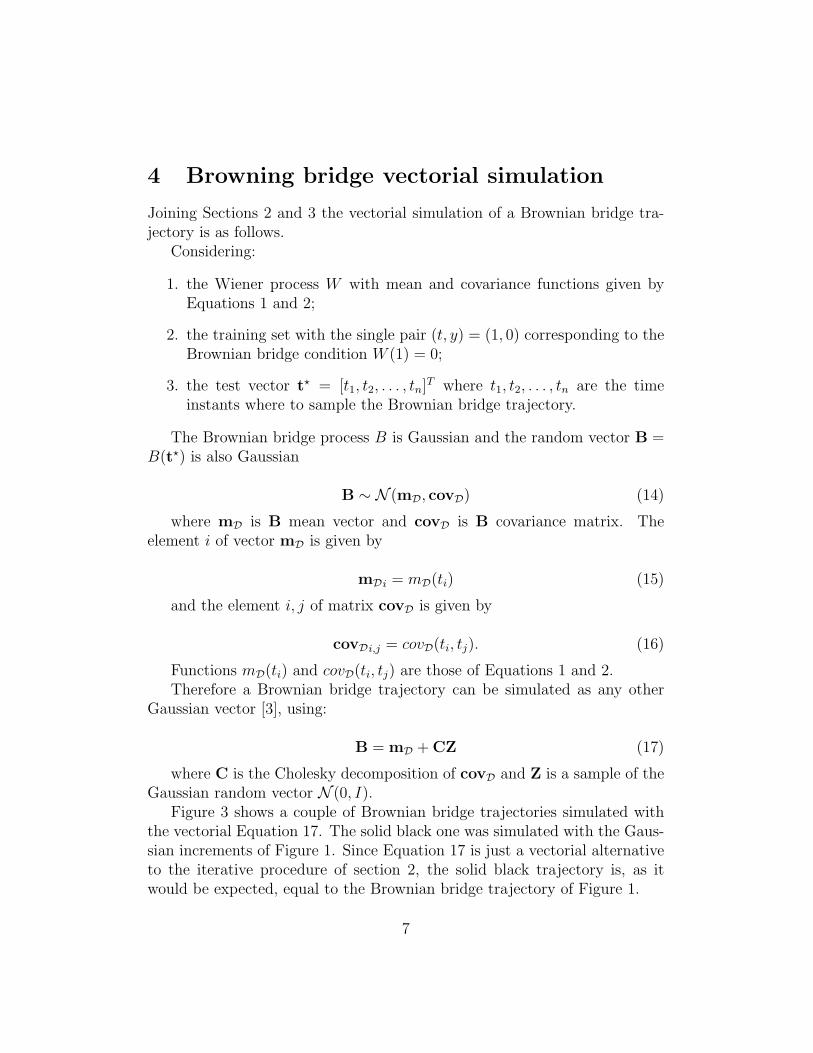
4 Browning bridge vectorial simulation

Joining Sections 2 and 3 the vectorial simulation of a Brownian bridge tra-jectory is as follows.

Considering:

1. the Wiener process W with mean and covariance functions given byEquations 1 and 2;

2. the training set with the single pair (t, y) = (1, 0) corresponding to theBrownian bridge condition W (1) = 0;

3. the test vector t? = [t1, t2, . . . , tn]T where t1, t2, . . . , tn are the timeinstants where to sample the Brownian bridge trajectory.

The Brownian bridge process B is Gaussian and the random vector B =B(t?) is also Gaussian

B ∼ N (mD, covD) (14)

where mD is B mean vector and covD is B covariance matrix. Theelement i of vector mD is given by

mDi = mD(ti) (15)

and the element i, j of matrix covD is given by

covDi,j = covD(ti, tj). (16)

Functions mD(ti) and covD(ti, tj) are those of Equations 1 and 2.Therefore a Brownian bridge trajectory can be simulated as any other

Gaussian vector [3], using:

B = mD + CZ (17)

where C is the Cholesky decomposition of covD and Z is a sample of theGaussian random vector N (0, I).

Figure 3 shows a couple of Brownian bridge trajectories simulated withthe vectorial Equation 17. The solid black one was simulated with the Gaus-sian increments of Figure 1. Since Equation 17 is just a vectorial alternativeto the iterative procedure of section 2, the solid black trajectory is, as itwould be expected, equal to the Brownian bridge trajectory of Figure 1.

7

ææ0.2 0.4 0.6 0.8 1.0

-1.0

-0.5

0.0

0.5

1.0

1.5HaL

ææ0.2 0.4 0.6 0.8 1.0

-1.0

-0.5

0.5

1.0

HbL

0.2 0.4 0.6 0.8 1.0

-1.0

-0.5

0.0

0.5

1.0

1.5HcL

Figure 3: Brownian bridge trajectories simulated with the vectorial Equation17: (a) training set; (b) regression function, two standard deviation confi-dence regression band (gray) and the not conditioned, mean centered, twostandard deviation band (light gray); (c) Brownian bridge trajectories.

8

(a) System

CPU Intel Core2 CPU 6300 1.86GHzMemory 4GB

OS Linux x86 (32bit)Language Mathematica 8.0.4.0

(b) Task

Simulation Brownian bridge trajectoriesNumber of trajectories 1000

Number of samples per trajectory 1000 (uniformly)

(c) Execution Times (in seconds)

Iterative 32.31sVectorial 3.49s

Table 1: Iterative and vectorial execution times comparison.

5 Execution time comparison

In order to compare the execution times of the iterative Brownian bridgesimulation procedure of Section 2 and the vectorial procedure of Section 4under an interpreted language framework, we implemented both using theMathematica 8 language [5] and tested the two alternatives on the task ofgenerating 1000 Brownian bridges sampled uniformly 1000 times.

Table 1 describes: (a) the execution system; (b) the task; (c) the executiontimes of both alternatives.

As it would be expected, the Brownian bridge vectorial simulation withthe Mathematica 8 language is faster than the iterative alternative. In theparticular case tested, approximately 10 times faster. As mentioned before,this is because vectorial operations are supported by built-in functions whichare implemented by optimized machine code.

9

6 Extensions

It is clear by the Brownian bridge vectorial construction that the simulationprocedure can be naturally extended in the following 3 ways:

1. considering a condition different from W (1) = 0 (either in the timeinstant and its value);

2. considering more than one conditions (sequences of bridges);

3. considering other Gaussian processes besides the Wiener process (con-sidering mean and covariance functions different from the Wiener pro-cess ones).

The first two ways were already illustrated by Figure 2(d) where therewere a total of four conditions, different from the Brownian bridge condition.

Regarding the third way Figures 4 and 5 illustrate the same example ofFigure 2, but now for geometric Brownian motion and Ornstein-Ulenbeckmean reversion process. We choose this two processes for their importancein modelling stock prices and interest rates, respectively. The simulationprocedure is the same of the example in Figure 2, except that the appropriatemean and covariance functions are used.

In the geometric Brownian motion case, the simulation was done for theunderlying log normal process, which is a Gaussian process with mean andcovariance functions given by:

m(t) =

(µ− σ2

2

)t (18)

and

cov(s, t) = σ2 min(s, t) (19)

where µ is the drift and σ the volatility. The geometric Brownian mo-tion trajectories were obtained by taking the exponential of the log normalones and multiplying by the process initial value x0. The values used in thesimulation examples of Figure 4 were: x0 = 0.5; µ = 1.0 and σ = 1.0.

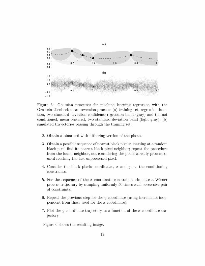
In the Ornstein-Ulenbeck mean reversion process case, the mean andcovariance functions are given by:

m(t) = x0e−kt + θ(1− e−kt) (20)

10

ææ

ææ

0.2 0.4 0.6 0.8 1.0

0.5

1.0

1.5

2.0

2.5HaL

0.2 0.4 0.6 0.8 1.0

0.2

0.4

0.6

0.8

1.0HbL

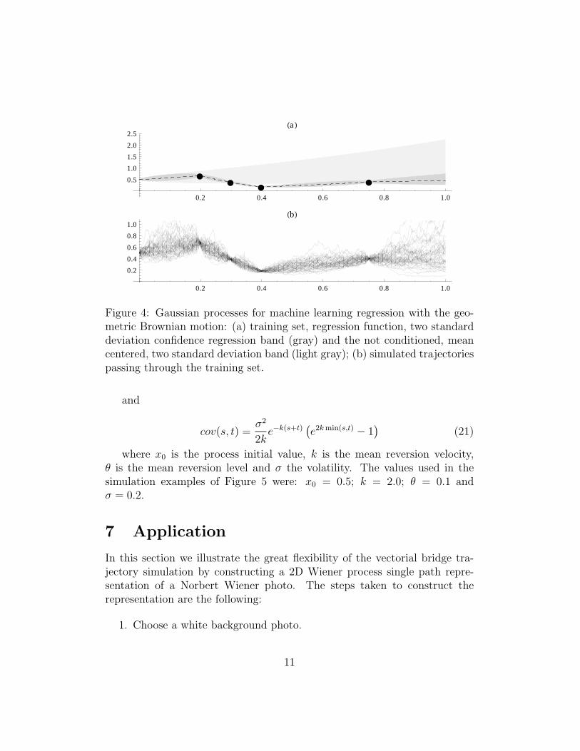
Figure 4: Gaussian processes for machine learning regression with the geo-metric Brownian motion: (a) training set, regression function, two standarddeviation confidence regression band (gray) and the not conditioned, meancentered, two standard deviation band (light gray); (b) simulated trajectoriespassing through the training set.

and

cov(s, t) =σ2

2ke−k(s+t)

(e2k min(s,t) − 1

)(21)

where x0 is the process initial value, k is the mean reversion velocity,θ is the mean reversion level and σ the volatility. The values used in thesimulation examples of Figure 5 were: x0 = 0.5; k = 2.0; θ = 0.1 andσ = 0.2.

7 Application

In this section we illustrate the great flexibility of the vectorial bridge tra-jectory simulation by constructing a 2D Wiener process single path repre-sentation of a Norbert Wiener photo. The steps taken to construct therepresentation are the following:

1. Choose a white background photo.

11

æ

æ

æ

æ

0.2 0.4 0.6 0.8 1.0

-0.4-0.2

0.20.40.60.8

HaL

0.2 0.4 0.6 0.8 1.0

-1.0

-0.5

0.5

1.0

1.5HbL

Figure 5: Gaussian processes for machine learning regression with theOrnstein-Ulenbeck mean reversion process: (a) training set, regression func-tion, two standard deviation confidence regression band (gray) and the notconditioned, mean centered, two standard deviation band (light gray); (b)simulated trajectories passing through the training set.

2. Obtain a binarized with dithering version of the photo.

3. Obtain a possible sequence of nearest black pixels: starting at a randomblack pixel find its nearest black pixel neighbor; repeat the procedurefrom the found neighbor, not considering the pixels already processed,until reaching the last unprocessed pixel.

4. Consider the black pixels coordinates, x and y, as the conditioningconstraints.

5. For the sequence of the x coordinate constraints, simulate a Wienerprocess trajectory by sampling uniformly 50 times each successive pairof constraints.

6. Repeat the previous step for the y coordinate (using increments inde-pendent from those used for the x coordinate).

7. Plot the y coordinate trajectory as a function of the x coordinate tra-jectory.

Figure 6 shows the resulting image.

12

Figure 6: 2D Wiener process single path representation of a Norbert Wienerphoto.

13

8 Conclusions

The contribution of the present paper is twofold:

1. it presents a vectorial alternative to the iterative simulation of Brown-ian bridge trajectories which is relevant regarding the execution speedof interpreted programming languages implementations;

2. it extends in a natural way the vectorial alternative to the class ofpath dependent Gaussian processes leading to a trajectories simulationvectorial framework of those processes.

References

[1] Quantlib - a free/open-source library for quantitative finance, 2012.

[2] Tomas Bjork. Arbitrage Theory in Continuous Time. Oxford UniversityPress, 2nd edition, 2004.

[3] Paul Glasserman. Monte Carlo Methods in Financial Engineering(Stochastic Modelling and Applied Probability) (v. 53). Springer, 2003.

[4] Carl E. Rasmussen and Christopher K. I. Williams. Gaussian Processesfor Machine Learning (Adaptive Computation and Machine Learning se-ries). The MIT Press, 2005.

[5] Inc. Wolfram Research. Mathematica edition: Version 8.0.4.0, 2011.

14