BROWN UNIVERSITY Department of Computer Science

Master's Project CS-89-M6

"Raster Algorithms for 2D Primitives"

by Dilip Da Silva

RASTER ALGORITHMS FOR 2D PRIMITIVES

submitted by

Dilip Da Silva

In partial fulfillmen t of the requirements for the Master of Science Degree

in Computer Science

Brown University May 1989

Andries van Dam, advisor

ABSTRACT

This thesis presents a coherent and uniform method for drawing single pixel outlines. These methods can be easily extended to scan more complex (thick and filled) primitives. Methods to clip both simple and complex primitives, consistent with the drawing methods discussed, are also presented. To achieve this aim, a comprehensive overview and discussion of modern algorithms to scan-convert 2D primitives such as lines, circles, standard ellipses, and general ellipses is included. In addition to the presentation of commonly known algorithms, this thesis also presents new and original algorithms to solve some problems inherent to existing algorithms.

TABLE OF CONTENTS

SUBJECT PAGE

ABSTRACT ,......................................................................... 1

I. INTRODUCTION 1

II. SCAN-CONVERSION 1

A. SINGLE-PIXEL OUTLINES 1 1. Scan-converting Lines 2 2. Scan-converting Circles 7 3. Scan-converting Standard Ellipses 1 3 4. Scan-converting General Ellipses 2 5

B. FILLED PRIMITIVES 3 5 1. Calculating Representation of Filled Primitive .. 3 5 2. Fill Patterns 3 5 3. Tiling 3 6

C. THICK PRIMITIVES 3 6 1. Replicating Pixels 3 6 2. Filling Areas Between Boundaries 3 7 3. Tracing The Outline With A Pen Tip 4 0 4. Thick Polyline Approximation 4 0 5. Patterned Thick Primitives 4 1 6. Border Styles 4 1

III. CLIPPING 4 3 A. CLIPPING LINES 4 4

1. Cohen Sutherland Algorithm 4 4 2. Nicholl, Lee and Nicholl Algorithm 4 9 3. Drawing The Clipped Line 5 2

B. CLIPPING CIRCLES 5 5

SUBJECT PAGE

11

C. CLIPPING STANDARD ELLIPSES

D. CLIPPING GENERAL ELLIPSES

E. CLIPPING THICK AND FILLED PRIMITIVES

F. CLIPPING TO WINDOWS THAT ARE NOT RECTANGLES

IV. SUMMARY

5 8

5 9

5 9

6 0

6 1

REFERENCES...................................... . i v

111

I. INTRODUCTION

This thesis presents a coherent and uniform method for drawing single pixel outlines. These methods can be easily extended to scan more complex (thick and filled) primitives. Methods to clip both simple and complex primitives, consistent with the drawing methods discussed, are also presented. To achieve this aim, a comprehensive overview and discussion of modern algorithms to scan-convert 2D primitives such as lines, circles, standard ellipses, and general ellipses is included. Among the algorithms are those to scan-convert single-pixel outlines of primitives, to draw thick and filled representations of primitives, and to clip primitives. In addition to the presentation of commonly known algorithms, this thesis also presents new and original algorithms to solve some problems inherent to existing algorithms. The discussion of scan-converting single-pixel outlines of primitives, for example, combines commonly known methods with the technique of partial differences. In the case of standard ellipses, this combination produces an algorithm that is more efficient than any published to date. This algorithm also solves a problem presented by previously published algorithms wherein drawing thin, long standard ellipses truncates the ends of the ellipse. Another important contribution is an algorithm that handles a II cases of general ellipses, including thin ellipses. Also presented are various techniques for drawing thick and filled primitives, including techniques that extend commonly known algorithms for drawing single-pixel outlines of primitives. The final discussion in this thesis focuses on methods for clipping all 2-D primitives under study.

II. SCAN-CONVERSION

A. SINGLE-PIXEL OUTLINES

Lines, circles and ellipses are useful 2D pnmltIves that are commonly invoked in rapid succession by interactive graphics applications. Hence, algorithms to scan-convert these primitives have to create visually pleasing images as well as be efficient. The basic task of scan converting a primitive involves selecting the appropriate pixels that approximate the continuous mathematical representation of the primitive on a fixed integer grid. In approximating the primitive, we need to choose a meaningful measure of error and then try to minimize the error. We start out using the value of the function as a means of deciding how close a pixel is to the primitive. This method·

I

works well for lines and circles, but is unreliable when used with ellipses. A better method, called the midpoint method, indicates on which side of the primitive the midpoint between two pixels lies and limits the distance between the pixel chosen and the primitive to one half the distance between two pixels. We shall use this method as a basis for the circle, standard ellipse and general ellipse algorithms.

Fig. 1. Pixel, P. surrounded by 8 adjacent pixels

In order to make the scan-conversion algorithms efficient, we avoid floating point arithmetic, and use incremental techniques to minimize the calculations required for each pixel plotted. The basic strategy of incremental scan-conversion algorithms is to choose the next pixel from the previously chosen pixel by determining which of the adjacent pixels lies closest to the curve being drawn. Figure 1 illustrates a pixel, P, surrounded by its 8 adjacent pixels, where the pixels are named by their relative geographical location. However, the choice of the next pixel can be reduced to only a pair of adjacent pixels depending on which octant the slope of the curve is in at the currently selected pixel. We define within which octant the slope of a curve lies by the slope of the curve and the direction in which we are tracking the primitive. If, for example, we are tracking a line with a slope of 1/2 and we are tracking the line from left to right, then we define the slope of the line to lie within the first octant. For the case when the slope of the curve lies in the first octant, the choice of the next pixel is reduced to the pair, E and NE. Furthermore, the calculations used to determine the closer pixel of the pair can be done incrementally. That is, the calculations done to choose the current pixel can be used to simplify the calculations for the choice of the next pixel.

1. Scan-converting Lines

The task of scan-converting a line involves selecting the pixels that best approximate the equation of the line,

f(x,y) = y - mx - b = 0 (L 1)

2

where m is the slope and b is the y-intersect. For simplicity, assume that the end points of the line segment fall on integer coordinates and that the slope of the line lies in the first octant, where x ~ y > O. Symmetry can be used to draw lines in other octants. Since the slope of a line m is constant, the choice of the next pixel in an incremental algorithm is always chosen from the same pair of pixels adjacent to the currently chosen pixel. In the case of a line with a slope in the first octant, the choice of pixels is between E and NE.

NE NE

(Xi,Yi) E Fig. 2a. Pixel P is currently Fig. 2b. Determining which selected and next pixel is pixel, E or NE, is closer to the chosen from E or NE. line.

The selection process at each pixel is illustrated in figure 2a. At the i th step pixel P has been determined to be closest to the line and we now want to decide whether pixel NE or pixel E should be chosen next. Some method is necessary to select which pixel, NE or E lies closer to the line. In figure 2b, the distances from the pixels, NE and E, to the line are denoted by ne' and e', respectively. By similar triangles, the ratio of ne' to e' is the same as the ratio of ne to e and hence the distances ne and e can be used as accurate indicators of which pixel, NE or E is closer to the line.

Bresenham's algorithm [BRES65] calculates the smaller of the distances, ne and e, using only integer arithmetic. The algorithm uses a decision variable d which at each step is proportional to the difference between ne and e. If d = e - ne > 0 then ne < e and pixel NE is closer and is set, otherwise e < ne and pixel E is set. Figure 2b

i thillustrates the step where pixel P at coordinate (xi,Yi) has been determined to be closest to the line and we now want to decide whether pixel ~E or pixel E should be chosen. From examination of

3

figure 2b, the distance ne is the Y coordinate, Yi + 1, of the pixel NE minus the Y coordinate of the line when the x coordinate is Xi + 1. The distance e is the Y coordinate of the line when the x coordinate is Xi + 1 minus the Y coordinate, Yi, of the pixel E. The distance, e and ne, are given by the following equations.

ne = Yi + 1 - m(xi + 1) - b (L2)

e = m(xi + 1) + b - Yi (L3)

Thus, e - ne = 2mxi - 2Yi + 2m + 2b - 1 (L4)

Assuming we are drawing a line from starting point (xs,Ys) to ending point (Xf,Yf), where both end points fall on integer coordinates and Xs ~ xf, then m = dy/dx, where dy = Yf - Ys and dx = Xf - xs' Also, using (xs,Ys) to solve for b in (Ll), b = Ys - mx s' After substituting dy/dx for m and Ys - mx s for b, in (L4), we have

Multiplying both sides by dx, we have

dx(e-ne) = 2xidy- 2Yidx + 2dy + 2Ysdx- 2dyx s - dx. (L5)

Since dx is positive, it does not change the sign of (e - ne) so we can use dx(e-ne) as the decision variable to determine which pixel should be the next pixel chosen. In addition, since all the terms on the right hand side of (L5) are integers, the decision variable can be calculated using only integer arithmetic. Therefore

(L6)

The equation of the decision variable can be further simplified by calculating it in terms of the previous decision variable di. Subtracting 1 from each index gives:

d i = 2xi_l dy- 2Yi-l dx + 2dy + 2Ysdx- 2dyx s - dx.

Subtracting di from d i+ 1 gives:

4

In the case of the pair of pixels, NE and E, we know that Xi = xi-l + 1. Hence

if di ~ 0 then pixel NE is chosen so Yi = Yi-l + 1 and

di+1 = di + 2dy - 2d x (L7)

if di < 0 then pixel E is chosen so Yi = Yi-l and

di+l = di + 2dy (L8)

Since the line starts out at (xs,Ys)' from (L6)

dl = 2dy - dx. (L9)

procedure LINE (Xs, Ys, Xf, Yf : integer) var dx, dy, const1, const2, ct, x, y integer;

begin dx := Xf - Xs; dy := yf - Ys; d := 2 * dy - dx; initial d from (L9)

const1 := 2 * dy; increment from (L8)

const2 := 2 * (dy - dx); increment from (L7) x : = Xs; y := Ys; setpixe1 (x, y) ; while x < X f do begin

x = x + 1; if d < 0 then ( choose pixel E )

d := d + const1 e1ae ( choose pixel NE )

begin y = y + 1; d := d + const2

end setpixel(x,y)

end {while} end

Fig. 3. Algorithm for drawing lines in the first octant

From the derivation above we have an incremental algorithm for drawing a line using minimal integer arithmetic per point plotted (see figure 3). This algorithm draws the bestfit approximation to a line. Another way of looking at the derivation of Bresenham's algorithm would be to examine the function of the line f(x,Y) = Y - mx - b. In the case of non-vertical lines, the function is positive for

5

coordinates above the line and negative for coordinates below the line. The line is defined by the points at which the function evaluates to zero. Since the function is linear, the evaluation of the function at any point is linearly related to the distance the point is from the line. Therefore, in figure 2b, if we compared the absolute value of the function at pixel NE with that at pixel E, the smaller value would be associated with the closer pixel. On examination of (L2), (L3), and (L4), this is exactly the situation in Bresenham's algorithm. However, this method does not extend well to non-linear functions like ellipses, where the value of the function of an ellipse increases more rapidly outside the ellipse than it decreases inside, hence becoming an unreliable indicator of distance from the curve. Therefore we shall describe a different method that does extend well to such non-linear functions. Piueway [PITT67] was the first to use this method and Van Aken [VANA84] later referred to it as the midpoint method. In order to choose the next pixel from a pair of adjacent pixels, instead of comparing the values of the function at the two pixels, this method evaluates the function at the midpoint between the two pixels. It then uses the value of the function at the midpoint to tell which side of the midpoint the function passes hence indicating which of the two pixels lies closer to the function.

Therefore, in the case of the line, instead of comparing the value of the function at pixel NE and at pixel E, the function is evaluated at the midpoint between pixel NE and pixel E. If the function evaluated at the midpoint is negative, then the line passes above the midpoint and pixel NE is closer. Conversely, if the function at the midpoint is positive then the line passes below the midpoint and pixel E is closer. If the midpoint falls exactly on the line, then both pixels, E and NE, are 1/2 the distance between two pixels from the line and either pixel can be chosen as the closer pixel. Using the same techniques as before, the algorithm can be written incrementally. A derivation of this algorithm was published by Van Aken and Novak [VANA85] and the resulting algorithm is exactly the same as Bresenham's algorithm.

In the case of lines that do not start and end at integer coordinate points, the starting pixel, (xs,Ys), is the rounded value of the starting coordinate point and the decision variable is initialized at (x s+l,ys+1/2). However, the algorithm has to implemented using floating point arithmetic since the values of dx and dy in (L6) may not be integers.

6

2. Scan-converting Circles

Scan-converting circles involves selecting the pixels that best approximate the equation of a circle.

f(x,y) = x2 + y2 - R2 = 0 (Cl)

represents a circle with radius R centered at the ongm. To simplify the algorithm we shall assume the circle is centered at the origin and shall draw only the arc of the circle that lies in the first octant. Other octants can be drawn trivially using symmetry and circles centered elsewhere can be drawn using a simple translation. Since only the arc in the first octant is considered and the slope of the arc stays within the third octant, the choice of the next pixel in an incremental algorithm is always reduced to the pair of pixels, Nand NW, relative to the currently chosen pixel.

I

~

~

I

I

\

i \

I I I

t

i I

~ NWi\ N

1\ (Xi,Yi)

I

mid P

point It.

I I

Fig. 4. Pixel P is currently selected and the next pixel is chosen from N or NW.

In figure 4, if pixel P has been determined to be the closest to the circle, we can use the midpoint method to determine whether pixel N or NW should be the next pixel set. The function f(x,y) given in (el) is negative for points inside the circle and positive for points outside the circle. The circle is defined by the points at which the function evaluates to zero. If the function at the midpoint between NW and N is negative, then the midpoint is situated inside the circle so pixel N is closer to the circle and should be set. On the other hand, if the

7

function at the midpoint is positive, then the midpoint is situated outside the circle so pixel NW is closer and should be set. In figure 4, the midpoint is inside the circle so pixel N should be the next pixel selected.

If P is located at (Xi, Yi) then the decision variable, which is the function of the circle evaluated at the midpoint between pixel NW and pixel N becomes

d = f( xi -1/2, Yi + 1) = ( Xi -1/2)2 + ( Yi + 1)2 - R2

In order to calculate the decision variable incrementally, instead of using the same techniques that we used for the line algorithm we shall use partial differences [PRAT85). If we define the partial difference Fn as

Fn(x,y) = F(x,y+l) - F(x,y),

where the subscript, n, represents a partial increment by one unit in the north direction, then every time we increment the evaluation point (xp, yp) of the function, F, by one in the positive y direction, to calculate the new value of the F at (xp' yp +1), we only have to add the value of Fn at (xp, yp) to the value of the F at (xp ' yp)' That is F(xp, yp+l) = F(xp' yp) + Fn(x p, yp). In the case of the equation of a circle,

Fn(x,y) = [x2 + (y+l)2 - R2] - [x2 + y2 - R2] = 2y + 1

Since the function of a circle is a second order function, the functions that define the first partial differences cannot be higher than first order functions. Consequently, the calculations needed to evaluate the partial differences are usually simpler than the calculations needed to evaluate the function itself. So we can evaluate the function at a partial increment from the current evaluation point by simply calculating the partial difference and adding it to the current value of the function. Furthermore, to simplify the calculations needed to evaluate the partial differences, we can again use partial differences. In the case of the first partial difference Fn, we define F u_ asu

8

where the second n in the subscript represents a partial increment of the evaluation point by one unit in the north direction. If the evaluation point, (xp' yp), of Fn is incremented by one in the y direction, we can calculate the new value of Fn at (xp' yp +1) by simply adding F _ to the previous value of Fn. Therefore, the newn n value of the function, F, at (xp,yp+1) can be calculated using the values of F and Fn at (xp' yp)' and then the new value of Fn at (xp' yp+1) can be calculated using the value of Fn and Fn_n at (xp' yp)' That is,

F = F + Fn Fn = Fn + Fn n

In the case of a circle, since the first partial differences, like Fn, are no higher than first order functions, the second partial differences, like F _ n, can be no higher than zero order functions. That is, then functions that define the second partial differences are all constants and hence do not have to be updated when the evaluation point changes. In the case of a circle,

Fn_n(x,y) = [2(y+l) + 1] - [2y + 1] = 2

As described above, we can define the other partial differences for partial increments in other directions. The partial difference Fnw ' for example, would represent an increment by one unit in the north direction and one unit in the west direction. In order to draw the arc of the circle that lies in the first octant, we initially set the current pixel, P, to the pixel at (R,O) (assume integer radii), which is the intersection of the circle with the positive x-axis. We then calculate the associated decision variable, d, at the midpoint between the pixel Nand NW. That is at the coordinate point (R-l/2,1). In addition, the values of Fn and Fnw have to be initialized at the same point, (R­1/2,1), as the initial decision variable. In order to decide which pixel, N or NW, is the next pixel chosen, we use the sign of the decision variable. If d < 0, then the midpoint is inside the circle and pixel N is chosen. In this case, the current pixel moves to the pixel N and so the corresponding evaluation point of the decision variable changes by one unit in the north direction. Using partial differences, we can updatf:; the decision variable by adding to it the current value of Fn ,

and then update the value of Fn by adding to it Fn_n. In addition, F n w has to be updated, so its value corresponds to the new

9

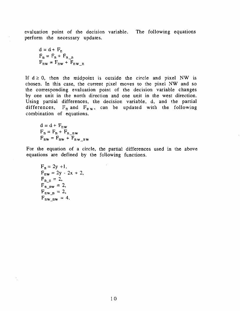
evaluation point of the decision variable. The following equations perform the necessary updates.

d =d+ Fn Fn =Fn + Fn_ n Fnw = Fnw + Fnw n

If d ~ 0, then the midpoint is outside the circle and pixel NW is chosen. In this case, the current pixel moves to the pixel NW and so the corresponding evaluation point of the decision variable changes by one unit in the north direction and one unit in the west direction. Using partial differences, the decision variable, d, and the partial differences, Fn and Fn w, can be updated with the following combination of equations.

d =d + Fnw Fn =Fn + Fn _nw

=Fnw Fnw + Fnw nw

For the equation of a circle, the partial differences used 10 the above equations are defined by the following functions.

Fn = 2y +1, Fnw = 2y - 2x + 2,

Fn_n = 2, F n_nw = 2, F nw_n = 2,

= 4.F nw_nw

10

procedure CIRCLE (R : real) var x, y : integer;

d, Fn, Fn_n, Fn_nw, Fnw, Fnw_n, begin

x := ROUND(R); y := 0: Fn := 3; Fn_n := 2; Fnw := 5 - 2 * x; Fnw n ;= 2; d := x * x - x + 5/4 - R * -R; while x >­ y do begin

setpixel (x, y) : y =­ y + 1; if d < 0 then

begin d := d + Fn; Fn := Fn + Fn_n; Fnw := Fnw + Fnw_n;

end el••

begi.n x - x-I; d := d + Fnw; Fn := Fn + Fn_nw; Fnw := Fnw + Fnw_nw;

end end (while)

end

Fnw_nw: real;

Fn_nw := 2; Fnw nw := 4: ( initial d from (C3) )

( choose pixel N )

{ choose pixel NW )

Fig. Sa. Algorithm to draw the arc of a circle (real radii) that lies in the first octant.

If R is an integer, then setting the current pixel to the pixel at (R,O), the values of d, Fn , and Fnw , are initialized at the coordinate point (R- 1/2,1). The initial value of d is

d1 = 5/4 - R (C2)

If R is not an integer, then setting the current pixel to the pixel at (Xo,O), where Xo is the rounded value of R, the values of d, Fn , and F nw , are initialized at the coordinate point ( Xo- 1/2,1). The initial value of d is

(C3)

The algorithm for real values is presented in figure 5a. If we restrict R to only integer values, then the algorithm can be implemented using only integer arithmetic. Using the initial decision variable d1

from (C2), we can substitute the new decision variable, h = d - 1/4 in the algorithm to eliminate the 5/4 fractional term in the initialization of d. The initial value of h will now be h = 1 - R. However, the comparison d < 0 will become h < -1/4. Since h can only take on integer values, the comparison h < 0 will have the same effect. The integer version of the algorithm is listed in figure 5b.

1 1

Fn_n := 2; Fnw_n := 2;

y ;= 0;

end end

procedure CIRCLE (R ; inteqer) var x, y, h, Fn, Fn_n, Fn_nw,

beqin x ;= R: Fn ;= 3; Fnw ;= 5 - 2 * R; h := 1 - R: while x >­ y do beqin

setpixel (x, y) :

y = y + 1: if h < 0 then

beqin d ;= d + Fn; Fn ;= Fn + Fn_n: Fnw ;= Fnw + Fnw_n:

end e18e

beqin x = x - 1; d := d + Fnw; Fn ;= Fn + Fn_nw; Fnw := Fnw + Fnw_nw:

end {while}

{ choose pixel NW }

{ choose pixel N }

Fn_nw ;= 2; Fnw_nw := 4; { initial d from (C2) }

Fig. 5b. Algorithm to draw the arc of a circle (integer radii only) that lies in the first octant.

It is interesting to note that if we used Bresenham's method to derive' the algorithm for a circle, we would arrive at the same algorithm with only the initialization of d being different. In the case of integer radii the initial value of d would be 3/2 - R instead of 5/4 - R. However, using the same kind of transformations as above, we can derive exactly the same algorithm. Therefore, in the case of integer radii, both algorithms draw exactly the same circle. In addition, Bresenham [BRES77] showed that in the ca~e of integer radii his algorithm draws the bestfit approximation to the circle.

McIlroy [McIL83] extensively examined the bestfit nature of Bresenham's circle algorithm and showed that In the case where the square of the circle's radius is an integer, Bresenham's algorithm draws the bestfit approximation to the circle. Although this may not be true for a circle algorithm that uses the midpoint method, the attraction of the midpoint method is that by definition the linear error of the curve drawn is bounded by 1/2. That is, the minimum distance between any pixel selected and the curve is never greater than half the distance between two pixels. Therefore, although the midpoint algorithm might not draw the bestfit approximation to a

1 2

b

circle In the case of real radii, the error will always be bounded by 1/2.

An optimization of the algorithm can be performed by noticing that for the arc of a circle in the first octant, pixel N is selected more often than pixel NW. This can be shown using simple geometry. If instead of using the partial differences, Fn and Fn w, we use Fn and Fw ' where Fw = -2x + 1. Then when pixel N is selected, the decision variable can be updated with the following sequence of equations.

d = d+ Fn Fn = Fn + Fn n

We do not have to update Fw because Fw_n = O. When pixel NW is selected, the decision variable is updated with the following set of equations.

d = d+ Fn + Fw

F n = Fn + Fn_nw Fw = Fw + Fw_nw

Therefore, only 2 additions are performed when pixel N is chosen, while 4 additions are performed when pixel NW is chosen. By shifting the computation ftom pixel N, which is chosen more frequently, to pixel NW, the average number of additions performed per pixel is reduced, producing a slightly faster algorithm.

3. Scan-Converting Standard Ellipses

Standard ellipses are the class of ellipses that are symmetric about the x and y axes.

y

a -_-:-ia r------+------+-- x

~-b

Fig. 6. A standard ellipse

1 3

They are described by the equation

(El)

where 2a is the diameter along the x axis and 2b is the diameter along the y axis. Again, to simplify the algorithm, we shall only draw the arc of the ellipse that lies in the first quadrant since other quadrants can be drawn trivially by symmetry. Also standard ellipses centered elsewhere can be drawn using a simple translation. The algorithm presented here is original in that it combines the approaches used by Van Aken[VANA84] and Kappel [KAPP85] along with using the technique of partial differences

Since the slope of the arc of the ellipse in the first quadrant changes continuously from one end of octant 3 to the other end of octant 4, we can divide the arc into two regions such that the slope in region 1 stays within octant 3 and the slope in region 2 stays within octant 4 (see figure 7). Thus for each region, the choice of the next pixel in an incremental algorithm is reduced to the same pair of pixels. In the case of region 1 the choice of pixels is between Nand NW, and in the case of region 2 the choice of pixels is between NW and W. The curve in each region can then be dr.awn using the same techniques that were used for the circle algorithm. However. we still need to determine when region 1 ends and region 2 begins.

y tangent

slope =-1

b t---__ ~

I component

-j--------------.L.-_xa

Fig. 7. Dividing the arc of the ellipse into two regions

14

Since the gradient of a curve at a point P on the curve is orthogonal to the tangent to the curve at p. we can use the gradient to determine when region 1 ends and region 2 begins. The boundary between the two regions is the point at which the slope of the curve is -lor equivalently. when the i and j components of the gradient are of equal magnitude.

grad f(x,y) = af/ax i + af/ay j = 2b2x i + 2a2y j

Therefore. by comparing the magnitudes of the two components, we can determine when we have left region 1 and entered region 2.

The function f(x.y) given in (E 1) is negative for points inside the ellipse and positive for points outside the ellipse. The ellipse is defined by the points at which the function evaluates to zero. In region 1, (figure 8a) if the current pixel P is located at (xit Yi), then the decision variable for region 1, d1, which is the function of the ellipse evaluated at the midpoint between pixel NW and pixel N, becomes

Region 1 Region 2

NNW

(Xi,Yi)

p w

I

NW

iexi,Yi)

i

Fig. 8a. Pixel P is currently Fig. 8b. Pixel P is currently selected and the next pixel selected and the next pixel is chosen from N or NW is chosen from NW or W

Again. we can use partial differences to calculate the rlecision variable incrementally. For region 1. the choice of pixels is between t-.'W and N. If d 1 < O. then the midpoint between NW and N is inside the ellipse and pixel N is chosen. Using the techniques for partial differences as developed for the circle algorithm, the difference

1 5

variable, dl, and the partial differences, Fn and Fnw , are updated as follows.

dl = dl + Fn Fn = Fn + Fn_n Fnw = Fnw + Fnw n

Otherwise, if dl ~ 0, pixel NW IS chosen and the difference variable is updated as follows:

dl = dl + Fnw Fn = Fn + Fn_nw Fnw = Fnw + Fnw nw

In region 2, the choice of pixels is between NW and W (figure 8b) and the decision variable for region 2, d2, is evaluated at the midpoint between NW and W. If d2 < 0, then the midpoint between NW and W is inside the ellipse and pixel NW is chosen. The difference variable, d2, and the partial differences, Fnw and Fw , are updated as follows.

d2 = d2 + Fnw Fw = Fw + Fw_nw Fnw = Fnw + Fnw nw

Otherwise, if d2 ~ 0, pixel W is chosen and the difference variable is updated as follows:

d2 = d2 + Fw Fw=Fw+Fw_w Fnw = Fnw + Fnw w

As for the case of circles, the function of a standard ellipse is a second order function. So the first partial differences are no higher than first order functions and the second partial differences are constants. For the equation of an ellipse, the partial differences used in the above equations are defined by the following functions.

= 2a2y + a2 , (E2)

= 2a2y + a2 - 2b2 x + b2 ,

= -2b2 x + b2 ,

1 6

Fn _ = 2a2,n

Fn_ = 2a2,nw F nw _n = 2a2 , Fnw _nw = 2a2 + 2b2, Fnw _w = 2b2, Fw_ = 2b2,nw Fw_ = 2b2,w

In region 1, we also have to compare the i and j components of the gradient to determine when we have entered region 2. The algorithm remains in region 1 while the magnitude of the j component is less than the magnitude of the i component. That is, while 2a2y < 2b2x. Fortunately, instead of computing the i and j components of the gradient, we can use the already calculated value of Fnw to determine when we have entered region 2. From the function of Fn w

in (E2), we notice that the inequality Pnw < a2+ b2 , is the same as the

inequality 2a2y < 2b2x.

When we leave region 1 and enter region 2 the decision variable changes from being evaluated at the midpoint between NW and N to being evaluated at the midpoint between NW and W. In order to simplify the computation involved in calculating from scratch the initial value of the decision variable, d2, for region 2, we can use value of the decision variable, d1, from the last step in region 1. The difference between the function evaluated at the midpoint, (xp,yp), between NW and N, and the midpoint, (xp-1/2,yp-l/2), between NW and W is given by:

Therefore, we can calculate the initial value of d2, which corresponds to f(x p-1/2,yp-1/2), from the value of d1, which corresponds to f(xp'yp)' as follows:

d2 = d1 - b2xp + b2/4 - a2 xp + a2 /4

Also, Fw and Fnw have to be initialized at (xp-l/2,Yp-1/2), the initial evaluation point of d2. Using (E2), the initial values of F and Fn ww are

17

Fw = -2b2xp + 2b2 ,

and Fnw = 2a2 yp - 2b2xp + 2b2,

In terms of the algorithm's variables, d2, Fw and Fn w , can be calculated with the following sequence of equations.

Fw = Fnw - Fn + b2

d2 =dl + ( Fw + Fw - Fn - Fn + b2 + 3a2)/4

Fnw = Fnw - a2 + b2

It is important to note that the location that the algorithm compares the i and j components of the gradient is at the location of the decision variable. If we used only the comparison of the two components to decide when region 2 was entered, we would sometimes enter region 2 early. Hence causing a pixel to be selected whose minimum distance from the curve may be greater than 1/2 the distance between two pixels.

Region 2

separating regions

Region 1

Fig. 9. Pixel P is currently selected with dl being evaluated in region 2. If a region change is made, so d2 is evaluated between NW and W. then erroneously NW will be the next pixel selected.

In figure 9, pixel P is currently selected, and the evaluation point of dl is in region 2, indicating a change in regions. The decision variable, d2, would then be initialized at the midpoint between NW and W, and the choice of the next pixel would be between NW and

18

W. However, if dl, which is the midpoint between Nand NW, is inside the eliipse, then the ellipse will pass above both Nand NW and, as in figure 9, it may pass more than 1/2 a unit distance above NW. Then using the criteria for region 2, we would erroneously select NW, a pixel that may be more than 1/2 a unit distance from the ellipse. This situation can be rectified by including a check to determine whether dl is inside the ellipse. Using the or operator, this check is done only after the test, (Fnw < a2+ b2), to compare the two components of the gradient fails. In figure 9, if dl were outside the ellipse, it may still pass above both NW and W. However, in this case, it can be shown that the ellipse cannot pass more than 1/2 a unit distance above NW and so will be less than 1/2 a unit distance from the ellipse.

The algorithm is started at (XO,O), where Xo is the rounded value of a, the intersection of the ellipse with the positive x-axis. The initial values of the decision variable, dl, Fnw ' and Fn , are calculated at the point (Xo-1/2, 1).

19

Fn nw .= a2Sq;

Fnw w "= b2Sq;

bSq; region 1 }

ELLIPSE (a, b : real) x, y : integer; dl, d2, aSq, bSq, a2Sq, b2Sq, aS~bSq, Fn, Fnw, Fw, Fn_n, Fn_nw, Fnw_n, Fnw_nw, Fnw_w, Fw_w, Fw nw : reaJ.;

begin x := ROUND (a) ; y := 0; aSq := a * a; bSq := b * b; a2Sq := aSq + aSq; b2Sq := bSq + bSq; aS~bSq := aSq + bSq; Fn :- a2Sq + aSq; Fn_n :~ a2Sq; Fnw := a2Sq + aSq - b2Sq * x + b2Sq; Fnw_n :- a2Sq; Fnw_nw :- a2Sq + b2Sq; Fw nw :", b2Sq; Fw w := b2Sq; dl-:- bSq * (x - 1/2) * (x - ::.12) + aSq - aSq * while (Fnw < aS~bSq) or (dl < 0) do begin

setpixel (x, y) ;

y - y + 1; if dl < 0 then ( choose pixel N )

begin dl := dl + Fn; Fn := Fn + Fn n; Fnw :- Fnw + Fnw n

end else ( choose pixel NW

begin x :- x - 1; dl := dl + Fnw; Fn := Fn + Fn nw; Fnw := Fnw + Fnw nw

end end (while)

procedure var

Fw : = Fnw - Fn + bSq; { change regions d2 := dl + (Fw + Fw - Fn - Fn + a~bSq + a2Sq)/4; Fnw :- Fnw + bSq - aSq;

while x ~ 0 do begin setpixel (x, y) ; x := x - 1; if d2 < 0 then

begin y := y + 1; d2 := d2 + Fnw; Fw := Fw + Fw_nw; Fnw .- Fnw + Fnw nw

end else

begin d2 := d2 + Fw; Fw := Fw + Fw w; Fnw := Fnw + Fnw w

end end (while)

end

( region 2 )

( choose pixel NW

( choose pixel W )

)

)

Fig. 10. Algorithm to draw the arc of an ellipse (real a and b) that 1ies in the fi rst quadrant

20

The complete algorithm is presented in figure 10. This algorithm is based on Van Aken's [VANA84] midpoint method algorithm but uses Kappel's [KAPP85] technique of using the gradient to determine a change in regions. It algorithm is an improvement over Van Aken's algorithm because unlike his algorithm, in order to determine a change in regions, it does not have to incrementally keep track of the decision variable for region 2 while traversing region 1. Kappel used the gradient to determine a change in regions, hence avoiding the additional arithmetic Van Aken's algorithm used to keep track of the decision variable for region 2 while traversing region 1. However, because his algorithm calculates the gradient at the nearest pixel, it sometimes enters region 2 one pixel too late. Hence causing a pixel to be selected whose distance from the curve may not be bounded by 1/2 the distance between two pixels. In addition, since his algorithm is incremental, the error caused by one pixel being displaced is propagated, causing other pixels to be selected whose distance from the curve may not be bounded by 1/2. Although, the algorithm in this paper, has more initialization overhead than Van Aken's algorithm, it uses fewer additions per pixel than both Kappel's and Van Aken's algorithms. Therefore, the efficiency of this algorithm becomes more evident for large ellipses.

Kappel Van Aken This paper

-I:

.S: 01) e.>

0::

N

NW

3

5

4

8

3

3

("l

I: .S: eo e.>

0::

NW

W

5

3

5

3

3

3

Fig. 11. Comparison of additions performed to keep track of decision variable for each pixel plotted.

In the case of integer a and b, the algorithm can be implemented using only integer arithmetic. The initial value of dl becomes

d11 = b2(-a + 1/4) + a2

2 1

procedure ELLIPSE (a, b : inteqer) var x, y, dl, d2, aSq, bSq, a2Sq, b2Sq, a4Sq, b4Sq,

a8Sq, b8Sq, a4S~b4Sq, Fn, Fnw, Fw, Fn_n, Fn_nw, Fnw_n, Fnw_nw, Fnw_w, Fw_w, Fw nw i.nteger;

beqin x :=- a: y := 0; aSq := a * a; a2Sq := aSq + aSq; a4Sq := a2Sq + a2Sq; bSq := b * b; b2Sq := bSq + bSq; b4Sq := b4Sq + b4Sq; a8Sq := a4Sq + a4Sq; b8Sq := b4Sq + b4Sq; a4~b4Sq := a4Sq + b4Sq; Fn := a8Sq + a4Sq; Fn_n:= a8Sq; Fn nw := a8Sq; Fnw := a8Sq + a4Sq - b8Sq * a + b8Sq; Fnw n : = a8Sq; Fnw nw := a8Sq + b8Sq; Fnw w := b8Sq; Fw_~w : = b8Sq; Fw_w := b8Sq; dl := bSq - b4Sq * a + a4Sq; while (Fnw < a4S~b4Sq) or (dl < 0) do begin region 1 }

setpixel (x, y); y ~ y + 1; if dl < 0 then { choose pixel N }

beqin dl := dl + Fn; Fn := Fn + Fn_n; Fnw := Fnw + Fnw n

end else { choose pixel NW }

beqin x := x-I; d1 := d1 + Fnw;

Fn := Fn + Fn_nw; Fnw := Fnw + Fnw_nw

end end {while}

Fw := Fnw - Fn + b4Sq; { change regions d2 := dl + (Fw + Fw - Fn - Fn + a4S~b4Sq + a8Sq)/4; Fnw := Fnw + b4Sq - a4Sq;

while x ~ 0 do beqin region 2 } setpixel (x, y) ;

x := x-I; if d2 < 0 then choose pixel NW

beqi.n y := y + 1; d2 := d2 + Fnw; Fw := Fw + Fw_nw; Fnw := Fnw + Fnw nw

end else { choose pixel W } beqin

d2 := d.2 + Fw; Fw := Fw + Fw_w; Fnw := Fnw + Fnw 'II

end end {while}

end

Fig. 12. Algorithm to draw the arc of an ellipse (integer a and b) that lies in the first quadrant

Using program transformations [SPR082], we can eliminate the 1/4 fraction by multiplying the above equation by 4. The new decision variable will then be 4 times the old decision variable. Therefore all

22

the equations used to calculate the old decision variable need to be transformed by multiplying them by 4. The integer version of the algorithm is presented in figure 12. While initializing d2, we perform an integer division by 4. We do not loose any precision by this division since the numerator consists of integer variables that are all multiples of 4. In fact, we could perform the division by doing a right shift by 2 bits.

1. Decision variable crosses ellipse 2. Region 1 exits when y value of current causing region 2 to be entered prematurely pixel equals b (top of ellipse)

\ y.

I /'" I~ I I

i ~V""i/

i : ­

I l.D cisior variable C:o~ses el ipse.

Ho\\ ~ver, ! Iince I camp<:pent 0 gradi~nt

is ne alive . I 1 . : r jot exi ~.regIo", IS

Also wher lcomponen isnel alive pixe Nis (~osenJ

I It

I I

! I I

I !I I

1\ /1\ ecision variable 1\ i

2. 1\Ulial

for lregior 2 I \I

I I I :

V I !

3.Ne t pixel chose~has /' T

It-(;oo dinatd less tl an ze 10 i

-endipg region 21 bop

.;t;.

I

I I

.1 I !

I I

Fig. l3a. Thin ellipse where decision Fig. 13b. Same ellipse, but i variable crosses ellipse causing ellipse to component of gradient is used so that be truncated tracking of ellipse is not truncated.

It is interesting to note that in the case of thin vertical ellipses, where the sides of the ellipse taper to less than a one pixel width, the algorithm truncates the ellipse. This is caused by the decision variable in region 1 jumping across the whole width of the ellipse and being evaluated on the opposite side. When this happens, the component of the gradient becomes negative and region 2 is entered prematurely. However, no pixels are selected while the algorithm is in the region 2 loop. Since the decision variable is on the opposite side of the ellipse, the x coordinate of the current pixel is equal to zero and after one iteration, the region 2 loop is exited (see figure 13a). This problem also occurs in both, Van Aken's and Kappel's

23

i

ellipse algorithms. We can rectify the situation in our algorithm by making the following changes to the algorithm in figure 10. Replace the test in the first while loop with

while ((Fnw < aS~bSq) or (dl < 0) or ((Fnw - Fn > bSq) and (y < b)))

and in the same while loop, replace the test condition for the if clause with

if ((dl < 0) or (Fnw - Fn > bSq))

If the decision variable has jumped across the ellipse, the i component of the gradient will be negative and hence will be less than the j component, which is positive, causing the test, (Fnw < a2+ b2 ), to fail. However, the test, (Fnw - Fn > b2 ), which has the same effect as comparing the i component of the gradient against zero, will be true, indicating that the i component is negative and that we are still in region 1 (see figure 13b). In the case of thin vertical ellipses, where the width of the ellipse is less than one pixel wide, the change in regions occurs at the top of the ellipse, close to where the ellipse intersects the positive y-axis. Therefore we will continue to track region 1 while the y coordinate of the current pixel is less than b, the intersection of the ellipse with the positive y-axis. The change in the condition clause of the if statement, forces the choice of pixel N if the i component is negative. Otherwise, the algorithm would pick pixels that would form a diagonal line crossing the y-axis into the second quadrant. Since the or operator is used to include the additional test for the while condition clause, it is only made when the region 1 loop is complete, or in the case of thin ellipses when the decision variable jumps across the ellipse. The additional test in the if clause is made only when dl is greater than zero, which on the average occurs less than half the time.

As in the case of the circle algorithm, we can again obtain a performance optimization of the algorithm by taking advantage of the fact that in region 2, pixel W is chosen more often than pixel NW. By using the partial differences , Fn and Fw instead of Fn and Fnw ' we can shift one addition for the computation done for pixel W, to the computation done for pixel NW, her.ce reducing the average computation per pixel plotted. We cannot take advantage of the corresponding change in region 1 because we would not have the value of Fnw to determine the change in regions. Hence, we would

24

have to use some other means to determine a change III reglOns, thereby increasing the computation.

4. Scan-converting General Ellipses

General ellipses are ellipses that do not have to be symmetric about the x and y axis. That is, they include all classes of ellipses, standard ellipses and standard ellipses that are rotated an arbitrary angle about their center. Although it is intuitively easier to define a general ellipse as a standard ellipse that is rotated an arbitrary angle, in order to derive the equation of a general ellipse, we shall present the mathematical definition of an ellipse. Given two points, Fl and F2, called the focal points of the ellipse, the ellipse is the set of points (x,y) such that the sum of the distances from (x,y) to the two focal points is equal to the constant 2a (figure 14a).

yy

-+-----------x

--+----f----I----X

L1 +L2=2a

Fig. 14a. General ellipse Fig. 14b. General ellipse centered at the origin centered at an arbitrary point

In the case of standard ellipses, the two focal points lie centered on the x-axis, and the a in the constant 2a is the same as that in (E1). Using simple geometry, we can derive the equation of a general ellipse that is centered at an arbitrary point. The equation is

f(x,y) = Ax2 + Bxy + Cy2 + Ex + Fy + D = 0, (Gl)

where the coefficients, A through F, are calculated using the focal points and the constant 2a. Equation (G 1) actually defines all conic sections, including parabolas and hyperbolas, where the values of the coefficients determine the conic section. To simplify the algorithm, we shall only draw general ellipses that are centered at the origin, since general ellipses centered elsewhere can be drawn using a

25

simple translation. In the case of general ellipses centered at the origin, the coefficients E and F equal zero, so the function becomes

f(x,y) = Ax2 + Bxy + Cy2 + D =O. (G2)

Also, in this case, the focal points are symmetrically located about the x- and y-axis. That is, if the focal point Fl is located at the coordinate point (Xr,Y r) then the other focal point, F2, will be located at (-Xr,-Yr) (figure 14b). Using the mathematical definition of the ellipse, the coefficients in (02) are defined in terms of the coordinate point of one of the focal points and the constant a.

A = a2 - X~ (G3) B = -2XrYr

2C = a - Y~ D = a2( X~ + Y~ - a2 )

I component

Fig. 15. Ellipse divided into 8 regions.

26

To further simplify the algorithm, we shall only draw the arc of the ellipse where the slope of the ellipse lies in the third through sixth octants. The other half of the ellipse can be trivially drawn by symmetry. Analogous to standard ellipses, we can divide the ellipse into eight regions, where we shall only draw the half-arc that includes the first four regions. The first four regions are defined such that the slope of the arc in region 1 stays within octant 3, the slope in region 2 stays within octant 4, the slope in region 3 stays within octant 5 and the slope in region 4 stays within octant 6 (see figure 15). Thus for each region, the choice of the next pixel in an incremental algorithm is reduced to the same pair of pixels. In region 1, for example, the choice of the next pixel is between Nand NW.

As for the case of standard ellipses, we can use the gradient to determine the boundaries between regions. The gradient of (G2) is given by

grad f(x,y) = af/ax i + af/ay j = (2Ax + By)i + (2Cy + Bx)j

The magnitudes of the i and j components can then be used to determine the boundary between two regions. The boundary between region 1 and region 2, for example, is the point at which the slope of the curve is -lor equivalently, when the i and j components of the gradient are equal and positive. Likewise, the boundary between region 2 and region 3 is the point at which the slope of the curve is horizontal or when the i component is zero and the j component is positive. Similarly, we can determine the boundaries between the other regions. Instead of comparing the magnitudes of the two components to determine a change in regions, as we did in the case of standard ellipses, we shall calculate the coordinate points of the boundaries between regions and compare the coordinate point of the current pixel against the boundary point to determine a change of regions. In region 1, for example, the choice of the next pixel is between Nand NW, and in either case the y-value of the current pixel increases by one. Therefore, we can determine when region 2 has been entered by comparing the y-value of the current pixel against the y-value of the boundary coordinate point. In order to determine the coordinate point of the boundary between region 1 and region 2, we calculate the inter~.ection between the line, 2Ax + By = 2Cy + Bx, determined by setting the i and j components of the gradient to each other, and the equation (G2) of the ellipse. However, the line, 2Ax + By = 2Cy + Bx, which passes through the origin, intersects the ellipse at two symmetrically located points. The point

27

that is the boundary between reglOn 1 and region 2 is the one at which both the i and j components are positive. The other point is the boundary between region 5 and region 6, where both the i and j components are negative. Therefore, by checking the sign of one of the components, we can determine which intersection point is the coordinate point of the boundary between region I and region 2. In a similar manner, we can calculate the coordinate points at the boundaries between the other regions. We also have to calculate the coordinate point of the boundary between region 8 and region 1, since this is the first pixel of region 1 and the starting point of the algorithm. In the algorithm, the coordinate points of the boundaries are named as in figure 15.

In order to describe a general ellipse in the most intuitive manner, we shall describe it as a rotated standard ellipse. Therefore, the parameters to our algorithm shall be the a and b parameters that describe a standard ellipse and an angle of rotation, theta. In a standard ellipse the focal points are located at (c,O) and (-c,O), where c 2 = a2 - b2. The focal points of the new ellipse are calculated by rotating the focal points, (c,O) and (-c,O), theta degrees. This is done by using a rotation matrix or equivalently sines and cosines. Once a focal point of the rotated ellipse is calculated, we can calculate the values of the coefficients to (0.2) and then the coordinate points of the boundaries between regions. When checking for a change in regions, instead of comparing the current pixel against the real value of the coordinate point at the boundary between regions, we shall use the rounded integer value of the coordinate point. This speeds up the algorithm, since an integer comparison is faster than a real comparison. As in the algorithm for standard ellipses, we shall use the method of partial differences to incrementally keep track of the decision variable. Also, when changing regions, we shall use the decision variable from the previous region to simplify the calculations needed to initialize the new decision variable.

In the case of thin ellipses, where the sides of the ellipse taper to less than one unit length, the decision variable may jump across the ellipse causing a streak of pixels to be selected that cross the ellipse and keep going until the boundary condition for the region is met (figure 16a). In order to rectify this problem, we can use the gradient of F, the function of the ellipse, to determine whether the decision variable has jumped across the ellipse. While selecting pixels in region 1, for example, in order for the decision variable to cross the ellipse and be located in either regions 3, 4, 5 or 6, it has to

28

i

have also crossed the line that passes from the boundary between region 2 and region 3 through the origin to the boundary between region 6 and region 7 (figure 16b). This line is determined by setting the i component of the gradient to zero. That is, 2Ax + By = O. When the decision variable is in regions 1, 2, 7, or 8, the value of the component is positive. When it crosses over into regions 3, 4, 5 or 6, the value of the i component becomes negative. The line is defined by the points at which the i component is zero. Therefore, by determining the sign of the i component at the evaluation point of the decision variable, we can determine if it has jumped across the ellipse. While the same test the ellipse.

selecting pixels in to determine if the

region 4, decision

by vari

symmetry, able has ju

we mped

can ac

use ross

line passing from boundary between re

2 and 3 to bOlmdary between r egions 6 gions and ~

1\ I ,\

\ \ \

I \ \ I,I

Ii \ \

I I ,I i\ \

I

I II

i i

\ I I \ I

II 1\,iI

I I

\\\

,

\\~

\\ \ !I

\' 'II \~\ 1 I

I ~\' I 1I

iII

I \\ ! \\,

Fig. 16a. Thin ellipse with major axis in Fig. 16b. Same ellipse, but if decision octant 3. While tracking region I, the variable crosses ellipse while tracking decision variable crosses ellipse causing region 1, pixel N is chosen to bring streak of pixels to be selected that are on decision variable closer or back to side opposite side of ellipse. being tracked.

Similarly, in regions 2 and 3, in order for the decision variable to cross the ellipse, it has to cross the line defined by setting the j component of the gradient to zero. When the algorithm determines that the decision variable has crossed the ellipse, it has to choose the pixel that is closer to the side of the ellipse it is tracking. While

29

selecting pixels in region 1, in order for the decision variable to jump across the ellipse, the ellipse has to be a thin ellipse and its major axis has to have a slope in the third octant. The major axis is the axis along which the width of the ellipse is the widest. In region 1 the choice of the next pixel is between Nand NW. When the deci~ion

variable is on the opposite side of the ellipse, pixel N will always be closer to the side of the ellipse the algorithm is tracking. In fact, choosing pixel N will tend to correct the problem of the decision variable being located on the opposite side of the ellipse by bringing the decision variable closer to or back to the side of the ellipse that is being tracked (figure 16b). In the case of the other regions, we can similarly determine which pixel to choose when the decision variable crosses the ellipse.

The first partial differences that are used in the algorithm are given by:

= 2Cy + Bx + C, (04) = 2Cy + Bx + C - 2Ax - By + A - B, = -2Ax - By + A, = -2Ax - By + A - 2Cy - Bx + C + B = -2Cy - Bx + C,

Again, as in the case of standard ellipses, the first partial differences are all first order functions, and so the second partial differences are all constants. The necessary second partial differences can be calculated from the equations above. Instead of keeping track of the appropriate component of the gradient to determine if the decision variable has crossed the ellipse, we can fortunately use the first partial differences. In region 1, for example, the choice of the next pixel is between Nand NW and so we have to keep track of the values of the first partial differences, Fn and Fn w' In order to determine if the i component of the gradient is less than zero, that is 2Ax + By < 0, we can use the comparison Fn - < -A + B. In the Fnw same manner, in the other regions we can avoid the computations needed to keep track of the appropriate component of the gradient by using the available partial differences.

The complete algorithm is presented in figure 17. The algorithm is original in that it combines existing methods. It uses the midpoint method to choose pixels while using the gradient technique to determine a change of regions. The technique of using the gradient to

30

solve the problem of thin ellipses, where pixels cross the ellipse, was originally suggested by Pratt[PRAT85]. The algorithm uses floating point arithmetic because the coefficients of the ellipse function are floating point numbers. One way to make the coefficients of the ellipse function integers, would be to restrict the focal points and the constant a to integer values. However, when a particular ellipse is rotated, in order to draw the new ellipse, the focal points have to be rounded to the nearest integer value, causing a slightly different ellipse to be drawn. Another method to speed up the algorithm would be to approximate the floating point values with integer values so that each of the inner loops for the regions consist of only integer arithmetic.

As in the case of standard ellipses, we could have used the comparison of the two components of the gradient to determine a change in regions. This would have eliminated the computations needed to calculate the three coordinate points of the boundaries between regions and we could avoid calculating the components of the gradient by using the available partial differences. However, in order to handle thin ellipses, the test condition to exit each region would be more complex. While tracking region 1, for example, the test condition for the while loop becomes

while «Fnw < (A-B+C» or (dl < 0) or «Fn - Fnw < cross!) and (y < Ytop»)

The first test, (Fnw < (A-B+C), in the while loop tests whether the decision variable has crossed the line that passes from the origin through the boundary point between region 1 and region 2. That is, it tests whether the j component of the gradient is not greater than the i component of the gradient. The second test, (dl < 0), is used only when the first test indicates a change in regions that is too early. This is similar to the test used for standard ellipses. The final test is used in the case of thin ellipses to determine if the decision variable has crossed the ellipse. If the decision variable has jumped across the ellipse, then the width of the ellipse at the point of the current pixel has to be less than one unit length. Therefore, the rest of region 1 is represented by a line and the end of region 1 coincides with the end of the line or the top of the ellipse. The top of the ellipse, Ytop, is calculated by first using the larger of the parameters, a and b, and the angle of rotation to represent the ellipse as a line segment and then calculate the top end point of the line segment.

3 1

The reason for not presenting this method as the algorithm of choice, instead of the method used in the algorithm in figure 17, is that in a small class of thin rotated ellipses, the comparison of the two components of the gradient is not an accurate indicator of a change in regions. This is caused by the fact that a change in regions using the comparison method is determined only when the decision variable jumps across the line that passes from the origin through the boundary between the regions. In a class of thin rotated ellipses, this dividing line between regions can be slopped such that the decision variable crosses the line a number of pixels too late. However, even this problem can be solved with additional tests in the test condition for the while loop. But then by increasing the arithmetic in the inner loops of the algorithm, we increase the arithmetic per pixel plotted, erasing the benefits obtained from not having to calculate the boundary points between regions.

32

procedure GENERAL_ELLIPSE (a, b, theta : real) var x, y, X:V, 'tV, YR, XH, XL : integer;

aSq,Xf,Yf,XfSq,YfSq,A,B,C,D,A2,B2,C2,B_2,kl,k2,k3,k4, Fn,Fnw,Fw,Fsw,Fs,Fn n,Fn nw,Fnw n,Fnw nW,Fw w,Fw nw,Fnw w,

Fw sw, Fsw w, Fsw sw,Fs ;;Fs ;;',Fsw ;; dl, d2-; d3, d4-; Xinit., Yinit-; XV~Yv,Xr,Yr,Xh,Yh,Xl.Yl,cr~ssl,c;;ss2,cross3,cross4real;

begin aSq := a * a; c :- sqrt(aSq - b * b) focal point to standard ellipse } Xf = c * cos (theta); focal point rotated theta degrees Yf = c * sin(theta); XfSq = Xi * Xf; YfSq = Yf * Yf;

A := aSq - XfSq; { Coefficients to (G2) } B := -2 * Xf * Yf;

C aSq - YfSq; D := aSq * (YfSq - A);

A2 :- A + A; B2 := B + B; C2 := C + c;

kl := -B/C2; { boundary point bet reg 8 and 1 } Xv :- sqrt( -D/(A + B*kl + C*kl*kl) ) ;

if (Xv < 0) then Xv := -Xv; Yv "= kl * Xv;

k2 .- -B/A2; { boundary point bet reg 2 and 3 } Yh :- sqrt( -D/(A*k2*k2 + B*k2 + C) ); if (Yh < O) then Yh := -Yh;

Xh .= k2 * Yh;

k3 .= (A2 - B)/(C2 - B); { boundary point bet reg 1 and 2 } Xr := sqrt( -D/(A + B*k3 + C*k3*k3) ); Yr := k3 * Xr;

if (Xr < Yr*kl) then Yr := -Yr;

k4 := (-A2 - B)/(C2 + B); { boundary point bet reg 3 and 4 } Xl :- sqrt( -D/(A + B*k4 + C*k4*k4) ); Yl :- k4 * Xl;

if (Xl> Yl*kl) than Xl := -Xl;

x:v .- ROUND (Xv) ; YV : = ROUND (Yv) ; { rounded boundary points } YR ROUND (Yr) ; XH "= ROUND (Xh); XL .= ROUND (Xl};

x := XIJ; { starting pixel } y := W;

Xinit :- x - 0.5; { initial evaluation point of decision variable } Yinit := y + 1;

Fn := C2*Yinit + B*Xinit + C; { initial Fn, Fnw and dl } Fnw = Fn - A2*Xinit - B*Yinit + A - B; dl := (A*Xinit*Xinit) + (B*Xinit*Yinit) + (C*Yinit*Yinit) + D;

{initialization of second order part.ial differences } Fn n "= C2; Fn nw := Fnw n "= C2 - B; Fnw nw .- A2 - B2 + C2;

Fw w := A2; Fw nw := Fnw w := A2 - B; Fsw_sw := A2 + B2 + C2; Fs s := C2; Fw sw := Fsw w := A2 + B; Fs sw := Fsw s .- C2 + B;-

(constants used in determining ~f decision variable has crossed ellipse } crossl ;= B - A; cross2:= A - B + C; cross3:= A + B + C; cross4:= A + B;

Fig. 17. Algorithm to draw half arc of general ellipse

33

while (y < YR) do begin { ----------------- REGION 1 ------------------ } setpixel (x, y) ; y := y + 1; if (d1 < 0) or (Fn - Fnw < cross1) than

beqin d1 := d1 + Fn; Fn:= Fn + Fn_n; Fnw := Fnw + Fnw_n;

end elae beqin

x := x - 1; d1 := d1 + Fnw; Fn := Fn + Fn_nw; Fnw := Fnw + Fnw_nw;

end and { ------------------------------------------------------------------- ­

{ Change Regions Fw :~ Fnw - Fn + A + B + B_2; Fnw := Fnw + A - C; d2 := d1 + (Fw - Fn + C)/2 + (A + C)/4 - A; while (x > XH) do beqin (----------------- REGION 2 ----------------- ­

setpixel{x,y); x := x - 1: if (d2 < 0) or (Fnw - Fw < cross2) than

beqin y := y + 1; d2 := d2 + Fnw; Fw:= Fw + Fw_nw: Fnw := Fnw + Fnw_nw;

end elae beqin

d2 := d2 + Fw; Fw:= Fw + Fw_w; Fnw := Fnw + Fnw_w; end

and { ------------------------------------------------------------------- ­{ Change Regions

d3 := d2 + Fw - Fnw + C2 - B; Fw := Fw + B; Fsw = Fw - Fnw + Fw + C2 + C2 - B; while (x < XL) do beqin {---------------- REGION 3 ----------------- ­

setpixel (x, y) ; x := x - 1; if (d3 < 0) or (Faw - Fw > cross3) then

beqin d3 :~ d3 + Fw; Fw:2 Fw + Fw_W; Fsw :~ Fsw + Fsw_w;

end elae beqin

y := y - 1; d3 :~ d3 + Faw; Fw:= Fw + Fw_aw; Fsw := Faw + Faw_aw;

end and ( ------------------------------------------------------------------- ­

{ Change Regions } Fs := Fsw - Fw - B; d4 := d3 - Faw/2 + Fa + A - (A + C - 8)/4; Fsw := Fsw + C - A; Fs := Fs + C - B_2: 'N := -'N; while (y > YV) do beqin ( ---------------- REGION 4 ------------------ }

setpixel (x, y) ; y := y - 1; if (d4 < 0) or (Fsw - Fs < cross4) then

beqin x := x - 1; d4 := d4 + Fsw; Fsw := Fsw + Fsw_sw;

end elae beqin

d1 := d1 + Fs; Fsw := Fsw + Faw_a; end

end ( ------------------------------------------------------------------- ­setpixel (x, y) ;

end { end GENERAL ELLIPSE f

Fig. 17. cont.

34

B. FILLED PRIMITIVES

The algorithms presented m the prevIOUS sections only draw single­pixel outlines of primitives. However, algorithms to draw filled primitives have many uses in 2D graphics applications. These algorithms can be divided into two tasks: calculating the pixels that form the filled primitive, and deciding with what value to fill each pixel.

1. Calculating Representation of Filled Primitive

The algorithms to scan-convert single-pixel outlines can be easily extended to draw filled primitives. Determining which pixels to fill involves intersecting successive row of pixels with the single-pixel outline to calculate the spans of adjacent pixels in each row that lie inside the filled primitive. Therefore, for the intersection of the primitive with a particular row, a span is characterized by a start pixel, which is the leftmost pixel of the single-pixel outline within the row, and an end pixel, which is the rightmost pixel of the single-pixel outline within the row. To draw the filled primitive, we fill each span that represents the primitive.

2. Fill Patterns

Once we have determined the spans that represent the filled pnmltlve, we can fill the spans with either a solid color or a pattern. Filling the primitive with a solid color involves simply setting each pixel within a span to the same color. However, filling the primitive with a pattern raises a number of issues. In the simplest case, the pattern is a bitmap, where this bitmap is repeated over the primitive. Calculating the value of a pixel within a span, involves first calculating the corresponding scanline within the bitmap that repeats over the span, and then calculating the corresponding bit within that scanline of the bitmap that represents the pixel to the colored. If we are using the bitmap as an opaque pattern, a 1 in the bitmap represent shading the pixel with the foreground color, and a 0 represents shading the pixel with the background color. On the other hand, if we use the bitmap as a transparent pattern, then only when the bit is aI, do we shade the pixel with the foreground color. An important issue in using patterns is how the pattern repeats over the primitive. That is, we need to know where the pattern is anchored to determine how the pattern repeats over the primitive or equivalently, which bit in the pattern corresponds to the pixel to be colored. One technique is to anchor the pattern to the primitive.

35

That is, the top-left pixel of the pattern is anchored to a particular pixel of the primitive. The advantage of this technique is that when we move the primitive, the pattern moves with the primitive. However, every time a primitive is drawn, we have to specify an anchor point. A second technique anchors the primitive to the window in which the primitive is being drawn. The disadvantage of this technique is that if the primitive is moved, the pattern does not move with the primitive. An interesting feature of this method is that primitives that are painted with the same pattern overlap and abut without any discontinuities in each primitives pattern.

3. Tiling

Instead of using a bitmap as a pattern, we can use a tile pixmap to tile the primitive. Here, we use the same technique as in patterns to index into the pixmap. However, instead of setting the pixel to be colored to either the foreground or background color, we set its color to the color of the corresponding pixel in the tile pixmap. In the case of a monochrome display, tiling is the same as using an opaque pattern, where the tile is a bitmap.

C. THICK PRIMITIVES

Thick primitives can be drawn using either of four methods. The first method is a crude approximation that replicates pixels in each column (or row) during scan conversion. The second method draws two copies of the primitive a thickness t apart and fills in the spans between the inner and outer boundaries. The third method traces the cross-section of the pen tip along the single-pixel outline of the primitive. The fourth method approximates primitives by polylines and then uses a thick line for each polyline segment.

1. Replicating Pixels

Here, instead of drawing one pixel per iteration of the inner loop of the scan-conversion algorithm, we draw multiple pixels. In the scan­conversion algorithm, if the choice of the next pixel is between two pixels that lie in the same column, for example E and NE, then we draw a stroke of pixels that lie in the column of the next pixel chosen and is centered on that pixel. Similarly, if the choice of the next pixel is between two pixels that line in the same row, the pixels are duplicated in rows. The thickness of the line is specified by the number of pixels replicated at each iteration of the inner loop. The advantage of this method is that it is very efficient. However, it does not produce the most visually pleasing thick primitives. In the case

36

of lines, the end points of the lines are restricted to vertical or horizontal edges. Furthermore, lines that are horizontal and vertical have a different true thickness from lines at an angle, where the true thickness of the primitive is defined as the distance between its boundaries perpendicular to the tangent of the primitive. This visual discrepancy becomes more apparent when we draw a circle or ellipse where the slope of the curve varies continuously. When drawing an ellipse, for example, the ellipse will appear thin where the slope of the ellipse is horizontal or vertical and will appe'ar thick where the slope of the ellipse is a diagonal.

2. Filling Areas Between Boundaries

This method draws a thick primitive as the approximation of the area that lies between the boundaries formed by stepping a distance t/2 on either side of the zero-width curve that is defined by the mathematical equation of the primitive. The strength of this method is that it is based on the intuitively correct definition of a thick primitive. However, when using this method, the extended boundaries of the thick primitives are not easily described by using only integer arithmetic. In the case of a line, a thick line is really the area enclosed by a rectangle or a rotated rectangle. Even if the end points of the line fall on integer coordinate points and the thickness, t, of the line is an integer, the end points of the bounding lines that define the thick line may not fall on integer coordinates. And since floating point arithmetic is needed to draw lines with end points that do not fall on integer coordinates, we need to use floating point arithmetic to select the pixels that define the bounding lines of a thick line. Therefore, in order to draw a thick line, we have to calculate the pixels that form the bounding lines of the thick line, and then, as in the case of filled primitives, use these pixels to calculate the spans form the thick line.

37

Arra

repr

]

Scanline from StanLeft to StopRight

Scanline from StartLeft to StopLeft and from StartRight to StopRight

]

Scanline from StartLeft to StopRight

I I I ~~ m

~«:

y entry ":~ , ~r~

:esenting Scanline - ,,<l ~ -::; , f!l: ....~

StanLeft _P""' ~

.. .. -­ ., ..... l- I-StopLeft ... ,....

--e l- I­ ~ f-' ...

StanRight -l,....-p :::: I-

StopRight - ID ~ W. ~'lS ~ W­ I f~ ~ ,:<:I ~

: r,il .....

~

.~ F~ ~:

Fig. 18. Thick circle with radius 8 and thickness 4, displaying scanline representation

In the case of a circle, a thick circle is the area enclosed by two concentric bounding circles. If the thick circle is defined by a radius R and a thickness t, then the inner bounding circle has a radius R-t/2 and the outer bounding circle has a radius R+t/2. Therefore, in order to draw the thick border of a circle, we scan-convert the single-pixel outlines of the inner and outer bounding circles. The pixels that represent these outlines are then used to calculate the spans that form the thick boundary. In fact, we only need calculate the spans that form on octant of the thick circle and then by symmetry calculate the spans that form the other octants.

A simple technique for calculating the spans of thick circles to use the pixels that form the inner and outer concentric circles to fill an array of entries that represent the scanlines that form the border of the thick circle. Figure 18 illustrates a circle with a radius of 8 and a thickness of 4, where the inner concentric circle has a radius of 6 and the outer concentric circle has a radius of 10. As illustrated, each array entry, representing a scanline, contains x-values of the start and stop pixels of the left border of the circle and the x-values of the start and stop pixels of the right border. The single-pixel outline of the outer concentric circle is used to fill in the values of StartLeft and StopRight. and the single-pixel outline of the inner concentric circle is used to fill in the values of StopLeft and StartRight. The array of

38

entries representing the scanlines are then used to draw the thick border of the circle, as illustrated in figure 18.

Fig. 19. Filled border of thick circle

Figure 19 illustrates the same thick circle as in figure 18, but with the area between the inner and outer concentric circles shaded. The pixels that form outer and inner concentric circles are shaded differently only for illustrative purposes. The thick border of the circle, therefore includes the pixels that form the inner and outer concentric circles, in addition to the pixels that lie in between the two concentric circles. If both, t/2 and R, are integers then the integer version of the circle algorithm can be used to select the pixels that form the bounding curves of a thick circle.

Unfortunately, in the case of standard ellipses, the bounding curves that are formed by moving a distance t/2 on either side of the curve of the ellipse are not concentric ellipses. However, concentric ellipses may be used to approximate a thick ellipse since the functions that define the actual bounding curves are 8th order functions [SALM96] and the task of selecting the pixels that outline these curves is computationally expensive. Therefore, to draw a standard ellipse with thickness t and with dimensions a and b, as defined in the section on standard ellipses, we need to calculate the pixels that form the area between the two bounding concentric ellipses where the inner bounding ellipse has dimensions a-t/2 and b-t/2, and the outer bounding ellipse has dimensions a+t/2 and b+t/2. Again, as in the case of thick circles, the task of drawing a thick ellipse can be accomplished by using an array of entries that encode the scanlines

39

that form the thick ellipse. The limit as the width of the ellipse goes to zero is the case where the outer and inner concentric ellipses coincide with the zero-width curve of the ellipse. Therefore, as the width goes to zero, the pixels selected for the thick ellipse are the same pixels as those selected for the single-pixel outline of the ellipse. Using this method precludes the situation where if we define a zero-width ellipse as not being visible (no pixels selected), then drawing an ellipse with a thin width may appear as an outline of the ellipse with gaps of pixels missing.

Since general ellipses are defined as standard ellipses that are rotated an arbitrary angle, in order to draw a thick general ellipse, the bounding concentric ellipses that define the thick standard ellipse are rotated and the pixels that lie between the two rotated bounding ellipses represent the thick general ellipse. Again, as in the case of thick standard ellipses, the task of drawing a thick ellipse can be accomplished by using an array of entries that encode the scanlines that form the thick general ellipse.

3. Tracing The Outline With The Pen Tip

This method uses a pen tip to trace the outline of the pnmlt1Ve. That is, a particular point of the pen tip follows the path of the single-pixel outline of the primitive. We can use pen tips of any shape, however circular pen tips produce the most visually pleasing thick primitives. The brute-force algorithm for drawing thick primitives using this method, is to draw the pen tip at each pixel of the single-pixel outline. However, since the pen tip overlaps at adjacent pixels, we will be setting pixels more than once. A better technique is to use the spans of the pen tip at each pixel of the single-pixel outline to compute the spans that form the thick primitive. This technique can be made more efficient by not using certain spans of the pen tip depending on the slope of the primitive and the shape of the pen tip. When a circular pen tip is used, this method produces the most accurate thick primitives. Also, this method is easily extensible to any primitive, including primitives with sharp corners.

4. Thick Polyline Approximation

All primitives can be "piecewise linearly" approximated by computing points on the boundary and then connecting these points with line segments to from a polyline. In order to closely approximate the primitive where the slope of the primitive varies

40

rapidly, the points must be calculated such that the points are closer together, and hence the line segments are smaller. Ellipses and circles, which are a class of ellipses, can be represented as two equations (one for the x and the other for the y value of the points that form the ellipse) that are each ratios of parametric polynomials [LIEN87]. This representation lends itself readily to such a piecewise­linear approximation of the ellipse. In order to draw the thick primitive, the individual line segments are then drawn as rectangles with specified thickness. Here however, the end points of the lines have to be joined smoothly.

Again, as in the case of all raster drawing algorithms, the choice of which definition of thick primitives to use and the choice of which algorithmic approximations to use between the speed of the resulting appearance of the primitive.

are dictated algorithm

by and

the trade-offs the visual

5. Patterned Thick Primitives

Once we have calculated the spans that represent the thick border of the primitive, as in the case of filled primitives, we can pattern or tile the spans that represent the border. In fact, we can draw filled primitives with thick borders, where the border is painted with one pattern and the region inside the border is painted with another pattern.

6. Border Styles

Another useful feature of 2D graphics applications, is the ability to draw primitives with various line styles. That is, using dashes to draw the border of the primitive. In the case of the single-pixel outline of a line, we can incorporate a mask of bits that describes the dashed style into Bresenham's line algorithm. Figure 20 illustrates using Bresenham's line algorithm for drawing dashed lines in the first octant.

41

procedure LINE(Xs,Ys,Xf,Yf, mask: integer) var dx, dy, const1, const2, d, x, y : integer;

begin dx := Xf - Xs; dy := Yf - Ys; d := 2 * dy - dx: const1 := 2 * dy; const2 := 2 * (dy - dx): x := Xs; y := Ys: if (low order bit of mask is a 1) than

setpixel (x, y) ; while x < Xf do begin

x - x + 1: if d < 0 then choose pixel E

d := d + const1 el.e choose pixel NE

begin y = y + 1: d := d + const2

end Rotate Right(rnask); ( rotate mask one bit to right)

-{ shifting low order bit into high order bit position if (low order bit of mask is a 1) then

setpixel(x,y); end {whilel

end

Fig. 20. Algorithm for drawing lines in the first octant

In the case of circles and ellipses, we can incorporate a similar mask into the scan-conversion routines to draw these primitives. However, since as in the case of a circle, only the pixels that form an octant of the circle are calculated and then the pixels for the other octants are drawn by symmetry, we have to draw the pixels in an order that is continuous around the circle. Otherwise, at the boundaries between octants, the dashed style may break down.

In the case of thick primitives, we can extend this method only if we use the pen tip method to draw a primitive. However, doing this does not produce visually pleasing dashed primitives. In the case of thick lines, a thick dashed line is really a number of filled rectangles or rotated rectangles that are spaced in a regular manner. Therefore, in order to draw a thick dashed line, we have to scan-convert one repeatable unit of filled rectangles depending on the dashed style, and then draw the line by simply translating this repeatable unit for the length of the line. If we are using the polyline approximation to draw· primitives, then we can use the dashed lines to draw the dashed polyline approximation. However, the dashes must be continuous from one segment to the next.

42

III. CLIPPING

Window ,----------:;.,.L-----,

,.,'" ,,,,

, ,, ,

",'" ",'"

Application ",'" '"

, " ~'"

Fig. 21. Clipping primitives to the application window

Another concern of raster drawing algorithms is that when a windowing system is employed, the primitives that are drawn by an application have to be clipped to the window that belongs to that application. In addition, the application's window may be obscured by several other windows requiring the primitive to be clipped to several rectangular areas. Therefore, in order for a primitive to be drawn in only the visible portions of the application's window, it may have to be clipped to several rectangular areas. There are several approaches to clipping. One approach to clipping is to perform the clipping in the drawing algorithm right before a pixel is set. In the case of an unobscured window, clipping is done only to the bounding rectangle of the window. Therefore, before a pixel is set, its coordinates are compared against the bounding rectangle of the window. If the pixel lies inside the window then it is set and if it lies outside the window it is not set. The comparison of a pixel located at (x,y) and a clip rectangle can be done by the following simple s tatemen1.

if ( (x ~ clip.left) and (x ~ clip. right) (y ~ clip.bottom) and (y ~ clip.top)

then setpixel(x,y);

In using this approach, the drawing algorithm still calculates all the pixels that represent tne primitive, but only sets those pixels that lie in the visible portion of the window.

43

In the case of multiple clip rectangles, we could perform the above comparison for every clip rectangle. However, the speed of the drawing algorithm would decrease as the number of clip rectangles increased. A better solution would be to keep a list of visible and invisible rectangles. When the current pixel goes outside the current clip rectangle, then the list would be traversed to find the new clip rectangle in which the current pixel lies. In addition, a flag would indicate if the current clip rectangle is visible or invisible and if it is visible then the current pixel should be set.

Although this approach is simple, it is inefficient when most or all of the primitive is located outside the window. This inefficiency arises because we calculate all the pixels that represent the primitive and then clip each pixel to the clip rectangle. A better approach would be to determine the visible and invisible sections of the primitive and then only draw the visible sections. Therefore, in order to clip a primitive, we need to calculate the end points of the sections that are visible and then be able to draw those sections.

A. CLIPPING LINES

In the case of line segments, the intersection of a line segment with the clip window can produce at most one line se"gment. Figure 22 illustrates a number of line segments that are clipped to a window.

.' ,..__.._.._.\t--:-=---..:.;..'-''-''-''-"-"----,

.' ..........

Application '. ' . ........Window ".

··,··

··· ···

I

,·,,· I I

Fig. 22. Clipping lines to the application window

1. Cohen-Sutherland Algorithm

In order to clip a line to a window, we then only have to calculate the end points of the visible segment and then draw the visible line segment. Cohen and Sutherland [NEWM79] developed an algorithm

44

that efficiently calculates these end points. The algorithm first determines if the line is completely inside the window, in which case we already have the end points of the visible segment, or if the line can be trivially rejected by checking if both end points lie on the outside halfplane of any edge of the window, in which case the line is completely outside the window. If neither of the above cases is true, then it divides the line into two segments such that one segment can be trivially rejected. It then proceeds to clip the remaining segment by applying the above two tests, and so on. This is repeated until the remaining segment is completely inside the window or can be trivially rejected.

outside halfpl~-:-1 ~outside halfplane of left edge of Right edge

\

outside halfplane 1000 1010 l-ofTOP edge

1001

Tovedge

Window :xl~ QQ'13 ~ 0001 0000 0010.:= II

.3 ~ II

Bonomedge Toutside halfplane

0110 of Bottom edge 0101 0100

Fig. 23. Extending edges of window to divide plane of window into 9 regions

In order to test whether the line is completely inside the window or lies in the outside halfplane of an edge, the edges of the window are extended to divide the plane of the window into nine regions (see figure 23). Each region is assigned a 4-bit code, where the code is determined by within which outside halfplane of the edges the region lies. The 4 bits in the code are assigned the following meaning:

First bit: outside halfplane of left edge. (left of left edge) Second bit: outside halfplane of right edge. (right of right edge) Third bit: outside halfplane of bottom edge. (below bottom edge) Fourth bit: outside halfplane of top edge. (above top edge).

45

Since the regIOn that lies above and to the left of the window, for example, lies in the outside halfplane of the left edge and in the outside halfplane of the top edge, it is assigned a code of 1001. Each end point of the line is then assigned the code of the region in which it lies. We can now use the codes of the end points to determine if the line lies completely inside the window or in the outside halfplane of an edge. From figure 23, it is clear that if both 4-bit codes of the end points are zero then the line lies completely inside the window. However, if both end points lie in the outside halfplane of a particular edge, then the codes for both end points will contain a set bit in the location that represents the outside halfplane of the edge. Therefore, if the logical and of the codes of the end points is not zero, then both end points must lie in the outside halfplane of one of the edges and hence the line can be trivially rejected.

D

Top edge

Window

,-------~~--------~---------------

Fig. 24. Subdividing line to determine visible segment

If the line is not completely inside the window or cannot be trivially rejected, we have to subdivide the line into two segments such that one segment can be thrown away. This is accomplished by using an edge the line crosses to cut the line into two segments. Then, the section that lies in the outside halfplane of the edge is thrown away. The line segment AD in figure 24, for example, crosses two edges, the top edge and the left edge. If we use the left edge to cut the line, we can then throwaway the segment CD that lies in the outside halfplane of thB left edge. We now have to apply the inside window and trivial rejection tests to the new line AC. The line still fails both tests. Since the line only crosses the top edge, we use the top edge to cut the line into two segments AB and BC. The segment BC is in the

46

outside halfplane of the top edge and hence is thrown away. Finally, the remaining segment AB is found to lie completely inside the window and is the segment that is drawn. We can determine which edges the line crosses by examining the 4-bit codes of the end points. If one end point is in the outside halfplane of the left edge, and the line failed the trivial rejection tests, then the other point has to lie on the inside halfplane of the left edge. So the line must cross the left edge. Therefore, if a line has failed the trivial rejection tests, then the bits that are set in the codes of its end points represent the edges the line crosses. However, if an end point is inside the window, we cannot use it to determine which edges the line crosses. Hence, we must use the code of an end point that is outside the window or equivalently, the code of an end point that is not zero. The full algorithm is presented in figure 25. The codes are defined as sets, for illustrative purposes.

Although this algorithm appears efficient, it is not the most efficient algorithm to clip lines. One problem with the algorithm is that every time it clips the line to the edge of the window, it recalculates the slope, m, of the line. However, this can be rectified by adding a test to check if the slope has already been calculated and only calculating it if it has not already been calculated. Another problem that is inherent in the algorithm is that the order of the edges it clips the line against makes a difference to the number of edges it clips against. That is, sometimes it clips the line to edges that it does not really have to clip against. In the line segment AD in figure 24, for example, if we first clipped the line against the left edge, then we would again have to clip it against the top edge. However, if we first clipped the line against the top edge, the remaining segment AB would be completely inside the window and we would not have to clip the line against any other edge. Therefore, in this case, clipping the line against the left edge is not really necessary.

47

var xLeft,xRight,yBottom,yTop : real: {clip rectangle of window}

procedur8 CLIP LINE(Xl,Yl,X2,Y2 : real} type edge-- (LEFT,RIGHT,BOTTOM,TOP);

code - set of edge: var Cl,C2,Cout code; x,y: real: accept,done boolean

procedur8 ENCODE(x,y real; var C : code}: begin

C := []; if x < xLeft then C := [LEFT] el.e if x > xRight then C := [RIGHT]; if x < yBottom then C := C + [BOTTOM] al.e if x > yTop then C := C + [TOP]

end

beqin ENOODE(Xl,Yl,Cl}; ENCODE(X2,Y2,C2); repeat

if (Cl = []) and (C2 = []) then {Line is inside window} beqin

accept := true: {trivially accept line} done := trua

end al.e if (Cl * C2) <> 1:] then (logical intersection of codes)

done := true (trivially reject line}

el.e (failed both tests} beqin

if Cl <> [] then (pick code of an end point} Gout := Cl: {than is outside clip recti

el.e Cout := C2;

if LEFT in Cout then begin (crosses left edge) x := xLeft; y := Yl + (Y2 - Yl) * (xLeft - Xl)!(X2 -Xl):

end el.e if RIGHT in Cout then begin (crosses right edge}

x :- xRight; y :- Yl + (Y2 - Yl) * (xRight - Xl)!(X2 -Xl);

end el.e if BOTTOM in Cout then begin {crosses bottom edge}

y :... yBottom; x :- Xl + (X2 -Xl) * (yBottom - Xl)!(Y2 - Yl);

end el.e beqin {crosses top edge} y := yTop: x := Xl + (X2 -Xl) * (yTop - Xl)!(Y2 - Yl):

end:

if Cout = Cl then Xl .= x: Yl "- y; ENCODE(Xl,Yl,Cl):

el.e X2 .= x; Y2 := y; ENCODE(X2,Y2,C2);

end until done;

if accept then DrawLine(Xl,Yl,X2,Y2): end

Fig. 25. Cohen-Sutherland Line-Clipping algorithm

48

2. Nicholl-Lee-Nicholl Algorithm

Nicholl, Lee and Nicholl [NICH87] developed a line clipping algorithm that avoids computing intersection points which are not end points of the final visible line segment and hence uses fewer arithmetic operations than the algorithm in figure 25. The algorithm works as follows. As before, the edges of the window are extended to divide the plane of the window into nine regions. There are three types of regions, corner regions, side regions and the region that is the window. We pick one end point, pI, of the line, and depending on within which type of region the end point lies, it subdivides the plane of the window as illustrated in figure 26.

Pl

LB

L

T

R

B

Pl L

LT i

LB:

LR

PI 10Cllled in corner region PI 10CIIled in window region PIIOCllled in side region

Fig. 26. Subdivision of the plane of the window depending on the type of region in which pI is located

The subdivisions are determined by dividing all positions of the end point, p2, such that each subdivision corresponds to intersections of the line with the same boundaries of the clip rectangle. In figure 26, the letters L,R,T and B stand for the left, right, top and bottom borders of the clip rectangle. In addition, any region that is bounded by solid lines and is labeled with a letter or a letters represents the subdivision where if p2 were located in that region, the line would cross the border(s) of the clip rectangle that the label indicates. If p2 is located in a subdivision that is not labeled, then we do not need to calculate any intersection points. That is, the line is either completely outside or completely inside the clip rectangle. Therefore, the algorithm first determines within which of the 9 regions the end point pI lies, and then depending on that region it determines the location of p2 among the appropriate subdivisions. The algorithm incrementally determines the subdivision within which p2 is located, by eliminating subdivisions that are easier to check to home in on

49

the correct subdivision. Once we have determined within which subdivision p2 is located, we can determine which borders of the window to clip against. In this way, only the necessary intersection points are calculated.

The algorithm in figure 27 illustrates the calculations of the intersection points when pI is in the top-left corner region. Note that the calculations (topproduct, leftproduct, etc.) performed for eliminating the easier subdivisions are reused to simplify the calculations for subdivisions that are not as easy to check. In addition, these calculations are also used again if we need to calculate any intersection points. By symmetry, we can derive the calculations of the intersection points when pI is in any of the other corner regions. We can also similarly derive the calculations if pI is located in a side region or the window region. Nicholl, Lee and Nicholl describe the computations for each type of region. Instead of deriving the calculations for each region that is of the same type, they use geometrical transformations and use the calculations for one of the regions in that type. If pI lies in the bottom-left corner region, for example, then we can use the calculations for the top-left corner region in figure 27 by reflecting both the line and the clip rectangle

\ about the x-axis and then using the fact that the reflected location of pI lies in the top-left corner region. When the final end points of the line are calculated, these end points are reflected back across the x­axis to give the end points (if any) of the line to be drawn.

var xLeft,xRight,yBottom,yTop : real; {clip rectangle of window}

procedur. CLIP_LINE (Xl,Yl,X2,Y2 : real) beqin

i~ Xl < xLeft than LeftColumn(Xl,Yl,X2,Y2,display) {-------->} el.e if Xl > xRight then RightColumn( ... ) {right column} el.e CenterColumn( ... ) {center column}

end

procedure LeftColumn(Xl,Yl,X2,Y2 : real; var display:boolean); beqin

if X2 < xLeft than display := fal.e; {Trivial reject} el.e if Yl > yTop than

TopLeftCorner(Xl,Yl,X2,Y2,display) {-------->} el.e if Yl < yBottom then BotLeftCorner( ... ); {bot-Left corner} el.e LeftSide( ... ) {Left Side}

end

Fig. 27. Nicholl-Lee-Nicholl Algorithm to clip line if pI lies in top left comer

50

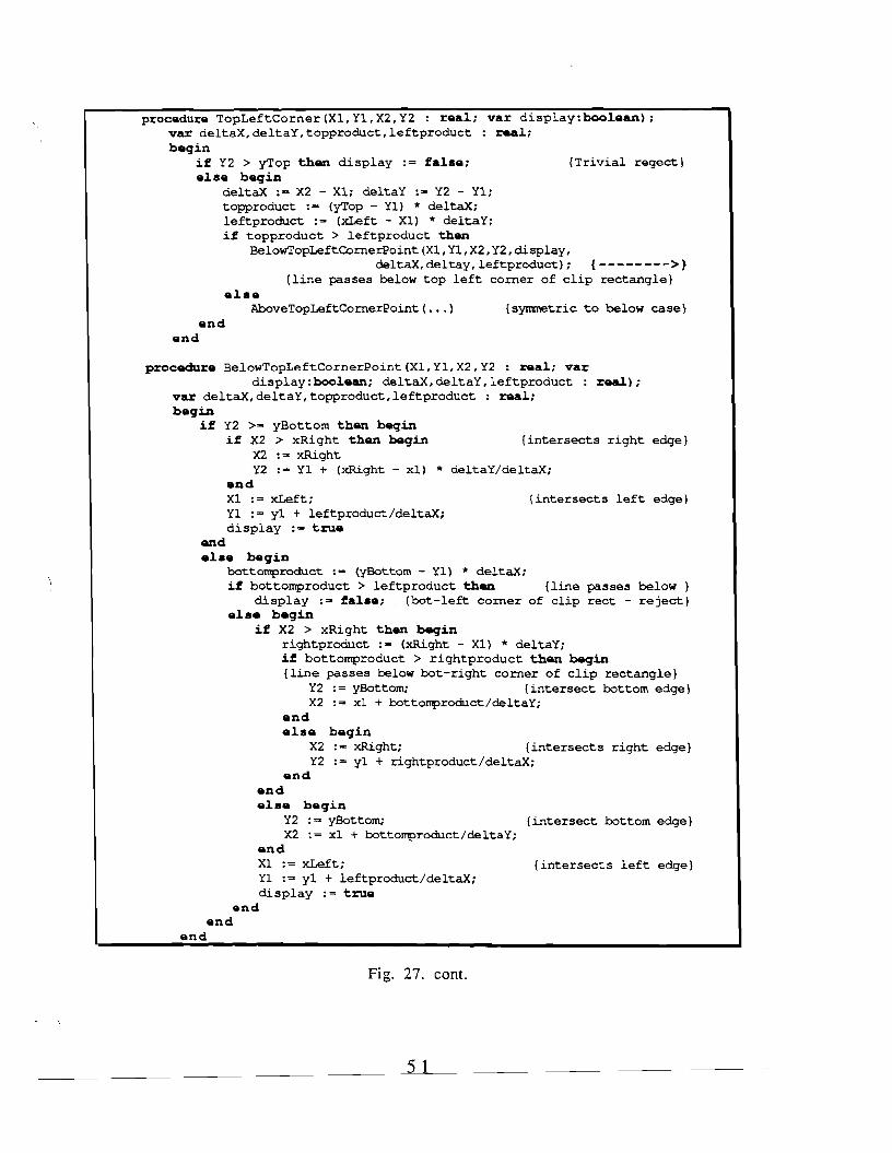
procedure TopLeftCorner(Xl,Yl,X2,Y2 : rea~: var display:boo~e&n):

var deltaX,deltaY,topproduct,leftproduct : rea~:

beqin if Y2 > yTop then display := fa~ae: (Trivial regect} e~ae beqin

deltaX :- X2 - Xl: deltaY :- Y2 - Yl: topproduct :- (yTop - Yl) * deltaX: leftproduct :- (xLeft - Xl) * deltaY: if topproduct > leftproduct then

BelowTopLeftCornerPoint(Xl,Yl,X2,Y2,display, deltaX,deltay, leftproduct): {-------->}

(line passes below top left corner of clip rectangle} e~ae

AboveTopLeftCornerPoint( ... ) {symmetric to below case} end

end

procedure BelowTopLeftCornerPoint(Xl,Yl,X2,Y2 : rea~; var display:boo~ean: deltaX,deltaY,leftproduct real):

var deltaX,deltaY,topproduct,leftproduct : rea~:

beqin if Y2 >- yBottom then beqin

if X2 > xRight then beqin {intersects right edge} X2 := xRight Y2 := Yl + (xRight - xl) * deltaY/deltaX;

end Xl := xLeft; {intersects left edge} Yl : = yl + leftproduct/deltaX; display :- true

end e~.e beqin

bottomproduct :- (yBottom - Yl) * deltaX; if bottomproduct > leftproduct then {line passes below }

display :- fal.e: {bot-left corner of clip rect - reject} e~ae beqin

if X2 > xRight then beqin rightproduct :- (xRight - Xl) * deltaY; if bottomproduct > rightproduct then beqin {line passes below bot-right corner of clip rectangle}

Y2 := yBottom; {intersect bottom edge} X2 := xl + bottomproduct/deltaY;

end e~ae beqin

X2 := xRight; (intersects right edge} Y2 := yl + rightproduct/deltaX;

end end e~.e beqin

Y2 := yBottom; (intersect bottom edge} X2 := xl + bottomproduct/deltaY;

end Xl := xLeft; (intersects left edge} Yl := yl + leftproduct/deltaX; display := true

and end

end

Fig. 27. cont.

5 1

3. Drawing The Clipped Line

Once we _have determined the end points of the visible line segment, we then have to draw the visible segment. The pixels selected to draw the line have to be exactly the same as the pixels that represent the original unclipped line. That is, if the window grows, and the whole line becomes visible, the section that becomes visible has to be drawn so it abuts the previous visible segment correctly. In addition, if the line is erased later, we cannot undraw pixels that are different from those originally set. The algorithms of the previous sections describe clipping a line to a clip rectangle and produce the end points of the segment that lies within the clip rectangle. If these end points have been clipped by one of the edges of the clip rectangle, then the end points can have real coordinates. We are faced with two problems: starting the line algorithm at a clipped (real) end point, and making sure we draw all the pixels from the original line that lie within the clip rectangle.

For a line with a slope in the first octant, for example, the line algorithm has to choose the next pixel from the pixels E and NE. It does this by choosing the pixel that lies closer to the line. We can accomplish the same result by taking the y-value of the line at the x­value of the two pixels, E and NE, and rounding it to determine the next pixel. Therefore, all the pixels that form a line can be calculated. by using the rounded y-value of the line for each integer x-value that spans the line. If a line with a slope in the first octant is clipped by the left edge, then the intersection of the line with the edge has an integer x coordinate, xleft, and a real y coordinate, (mxleft + b). And the pixel at the left edge (xleft, ROUND(mxleft + b)) is one of the pixels of the original unclipped line. If we start our incremental line algorithm at a pixel that lies on the original line and initialize the decision variable correctly, then all the other pixels selected for the rest of the line will be the same pixels that form the original unclipped line. In order to initialize the decision variable for a line with a slope in the first octant, if the first pixel is (xp,yp), then we simply calculate the decision variable at the midpoint between the pixels E and NE or equivalently at (xp+l,yp+l/2).

The second problem of making sure we draw all the pixels of the unclipped line that lie inside the clip rectangle is not evident when a line with a slope in the first octant is clipped by only vertical edges.

52

However, when the same line is clipped by a horizontal edge, there may be multiple pixels that form the line along the horizontal edge. (see figure 28). When we clip the line, the clipped end point has a real x coordinate, (ybot - b)/m, and an integer y coordinate, ybot. Although we can show that the pixel at (ROUND«ybot - b)/m), ybot) is a pixel that lies on the original unclipped line, this pixel may not be the leftmost pixel of the span of pixels shown. From the figure and the midpoint method, it is clear that the leftmost pixel is the one that lies just above the place on the grid where the line first crosses above the midpoint y = ybot - 1/2. Therefore, we simply find the intersection of the line with the line ybot - 1/2 and take the ceiling of the x-value. That is, we start the algorithm at (CEILING(ybot - 1/2 -b)/m), ybot). We run into the same problem if the line is clipped by the top edge, however, in this case we are calculating the ending pixel of the line. Here we clip the line to ytop + 1/2 and the ending pixel is the FLOOR of the intersection points x-value.

ClipLeft

ClipBottom

(Xs.Ys)

Fig 28. line with a slope in the first octant that is clipped by a horizontal edge

To summarize, if we are clipping a line with a slope in the first octant against the clip rectangle (ClipTop, ClipLeft, ClipBottom, ClipRight), then we use one of the clipping algorithms presented in the previous section and clip the line against the clip rectangle (ClipTop + 1/2, ClipLeft, Clipbottom - 1/2, ClipRight). The clipping algorithm returns the real-valued start point (Xs,Ys) and the real-valued end point (Xe,Ye) of the clipped line. The starting pixel (XS,YS) and the x coordinate of the ending pixel XE are calculated as follows:

XS := CSILING(Xs); YS := ~OUND(Ys);

XE := "LOOR(Xe};

53

We only need the x coordinate of the ending pixel to calculate how many pixels to draw. By symmetry, we can solve the same problem that occurs when lines with a slope in the second octant are clipped by the left and right clip edges. In this case, we clip the line against the clip rectangle (ClipTop, ClipLeft - 1/2, ClipBottom, ClipRight + 1/2). The starting pixel (XS,YS) and the y coordinate of the ending pixel YE are calculated as follows:

XS := ROUND(Xs); YS := CEILING1Ys); YE := FLOOR(Ye);

If all the end points of lines are restricted to integer values, then we can use the inner loop of the algorithm in figure 3 to select the pixels for the rest of the line. However, in order to calculate the initial decision variable with the constants, dx and dy, we have to use the end points of the original unclipped line. Again, the pixels selected will be exactly the same pixels that would represent the original unclipped line. The algorithm to draw the visible portion of a line with integer end points and with a slope in the first octant is given in figure 29.

var begin

dx := Xf - Xs; dy := Yf - Ys; const1 := 2 * dy; const2 := 2 * (dy - dx); x :- CEILING(xs); y : = ROUND (ys) ; Xend : = FLOOR (xf) ; d := 2*dy*(x - Xs) - 2*dx(y - ~s);

setpixel (x, y) ; while x < Xend do begin

x = x + 1; if d < 0 then

d := d + const1 el.e

begin y = y + 1; d := d + const2

end setpixel(x,y)

end {while} end

procedure LlNE(Xs,Ys,Xf,Yf: integer; xs,ys,xf,yf : real;)

dx, dy, const1. const2. d,

choose pixel NE

choose pixel E

{end points of original line} {end points of clipped line}

x, y, Xend: integer;

Fig. 29. Algorithm for drawing the visible portion of lines with a slope In the first octant and with integer end points.

54

---------

B. CLIPPING CIRCLES

In the case of circles the task of clipping a circle is more complex because the primitive could intersect the window at more than two points causing multiple segments to be visible. In order to clip a circle, we first should check if the bounding square of the circle intersects the clip rectangle. If the bounding square is completely inside the clip rectangle, then the whole circle is visible. On the other hand, if the bounding square is completely outside the clip rectangle, then the circle is outside the window and is not visible. If the bounding square partially intersects the clip rectangle, then the circle mayor may not be partially visible. Once we have determined that the bounding square partially intersects the clip rectangle, we can continue clipping the circle by dividing the circle into quadrants, where each quadrant is bounded by a square. We then check if the bounding squares of the quadrants intersect the clip rectangle. If the bounding square of a quadrant lies completely inside the clip rectangle, then the curve of the circle that lies in that quadrant is completely visible and hence is drawn. If you recall, the algorithm to draw a circle only calculates the pixels for one octant and we have to use symmetry to plot the pixels in the other octants. If the bounding square of a quadrant lies completely outside the clip' rectangle, then the curve of the circle that lies in that quadrant is outside the window and hence does not have to be drawn.

Bounding square of circle Bounding square of quadrant

2: ,------------~ o :__\ .t R

..J2R:r----,fiC--i

R '--""'---'- - - - ­ I Bounding

,----------- , rectangles : : ~ of octants[2

Fig. 30. Bounding box of circle, quadrant and octant

If the bounding square of the quadrant partially intersects the clip rectangle, we can further divide the curve of the circle that lies in the quadrant into octants (see figure 30) and then intersect the

55

bounding rectangles of the octants with the clip rectangle to determine if the curve in the bounding rectangle is completely visible or not. Finally, if the bounding rectangle of an octant partially intersects the clip rectangle, we can then draw the curve in the bounding rectangle by clipping each pixel to the clip rectangle. If the circle is very large, clipping each pixel of the curve that lies in the bounding rectangle of an octant may be expensive. A better method is to find the pixels that are the end points of the visible section of the circle in the octant and draw the pixels from one end point to the other. When we clip the bounding rectangle of an octant against the clip rectangle, we can also determine which edges of the clip rectangle intersect the bounding rectangle of the octant. We then intersect these edges with the curve of the circle to determine the intersection points of the edge with the circle. The intersection, for example, of the left edge of the clip rectangle, which is defined by the equation x = xLeft, with a circle centered at the point (Xc,Yc), which is defined by the equation (x-Xc)2 + (y-Yc)2 - R2 = 0 is calculated by substituting xLeft for x in the equation of the circle and solving for y. That is,

x = xLeft

and y =-Yc ± -VR2 - (xLeft + Xc)2.

If the term in the square root is negative, then the edge does not intersect the circle. However, since we are only checking edges that intersect the bounding rectangle of the curve in the octant, the edge has to intersect the circle and it can intersect the circle at at most two points. We then check each intersection point, to see if it lies on the boundary of the clip rect and within the bounding rectangle of the octant. In addition, since an edge can intersect the curve of a circle in an octant at only one point, if we find that the first intersection point satisfies these conditions, then we do not have to check the other point.

Furthermore, since only at most two borders of the clip rectangle can intersect the curve in the octant, once we have found two intersection points, we do not have to check the remaining edges. Figure 31 illustrates how to calculate the end points of the visible section of the curve in an octant. If we have a representation of the pixels that form an octant of the circle in memory I we can then use the end points to determine which pixels to set. That is, if only one border of the clip rectangle intersects the curve in the octant, we

56

determine the nearest pixel to the intersection point and then plot all the pixels of the curve in the octant that are in the inside halfplane of the edge. On the other hand, if two borders intersect the curve, then we determine the nearest pixel to one intersection point and plot all the pixels of the the octant that are in the inside halfplane of both edges. If no borders intersect the curve then we do not plot any pixels. In using. this method, we only calculate the pixels that form an octant of the curve when some or all of the circle is visible in the window, and we only have to perform these calculations once. If we do not have a representation of the pixels that form an octant in memory, we can calculate the pixels that only form the visible section of the octant.

, left boundary clip rect :

3. use intersection of clip rect "-.... points that are endpoints of

(Xl.Yl) visible section ofintersection

~~~--.--------------------~--------~ curve to draw thepoints of left m, ~ edge and circle visible section. <Xb.Yb)edge " bounding reet :

of octant : :'

""" ---~'!~'

"'-., ... _~-_ .... ", ~I E (D:"

2. if intersection point is on boundary of clip 1. Left and bottom edges of clip

reet and within bounding reet of octant then reet intersect bounding reet of

it is an endpoint of visible section of curve. octant

Fig. 31. Calculating the end points of the visible section of an octant of the circle that panially intersects the clip rect.

For the specific example of figure 31, the algorithm to draw the visible section is given in figure 32. Note that when a vertical edge clips the first octant of the circle, there may be multiple pixels that form the circle and lie along the vertical edge. We have to make sure that all the pixels of the original unclipped circle that are within the clip rectangle are drawn. This situation is the same as that when a line with a slope in the second octant is clipped by a vertical edge. Using the same reasoning as in the case of clipped lines, for the example in figure 31, we can solve this problem by intersecting the circle the the clip edge xLeft - 1/2 instead of xLeft. The y-value of the last pixel within the clip rectangle is then FLOOR of the y-value of the intersection point. We therefore, modify the clip rectangle by changing the left edge to xLeft - 1/2 and changing the right edge to xRight + 1/2. (Xb,Yb) and (XI,YI) are the intersection points of the

57

curve in the octant with the bottom and left edges of the modified clip rectangle, respectively. The algorithm is started at the pixel (XB,YB), which is the rounded value of (Xb,Yb) and the decision variable and partial differences are initialized at (XB-l/2,YB+l). The algorithm stops when the y-value of the current pixel equals the FLOOR ofYl.

procedure CIRCLE (R, Xb,Yb,Xl,Yl: rea~)

var x, y, Yend: integer; d, Fn, Fn_n, Fn_nw, Fnw, Fnw_n, Fnw_nw, xinit,

begin x :- ROUND (Xb) ; y : = ROUND (Yb) ; Yend :- FLOOR (Yl); xinit :- x - 1/2; yinit :- y + 1; Fn := 2* (yinit) + 1; Fn_n :- 2; Fnw := 2*yinit - 2*xinit + 2; Fnw_n:= 2; d :- xinit*xinit - yinit*yinit - R * R; whi~e y <- Yend do begin

setpixel(x,y}; y - y + 1; if d < 0 then

begin d :- d + Fn; Fn := Fn + Fn_n; Fnw :- Fnw + Fnw_n;

end el..

b.gin x = x - 1; d := d + Fnw; Fn := Fn + Fn_nw; Fnw := Fnw + Fnw_nw;

end end {while}

end

yinit: real;

Fn_nw := 2; Fnw nw := 4

{ choose pixel N }

{ choose pixel NW }

Fig. 32. Algorithm to draw the visible section of curve in figure 31

C. CLIPPING STANDARD ELLIPSES

In the case of standard ellipses, we can use the same method as for circles. The bounding rectangle of the ellipse is defined by the constants, a and b, from the equation of the ellipse. However, since a standard ellipse is symmetric by quadrants, we can only divide the bounding rectangle of the ellipse to the level of quadrants. As in the case of octants for a circle, when a quadrant partially intersects the clip rectangle, we can use the edges of the clip rectangle to calculate the intersection points of the border of the clip rectangle with the curve in the quadrant. These points can then be used to determine which pixels of the curve in the quadrant should be set.

58

D. CLIPPING GENERAL ELLIPSES

In the case of general ellipses, the bounding rectangle is defined by the terms Yh and Xv from figure 15. Since all general ellipses are not symmetric by quadrants, we cannot further divide the bounding rectangle into quadrants. However, since we can calculate the end points of regions, as in the algorithm to scan-convert general ellipses, we can divide the bounding rectangle of a general ellipse into rectangles, where each rectangle bounds the curve of the ellipse in one region. In the case of thin general ellipses, it is possible for a bounding rectangle of one region to overlap the bounding rectangle of another region. Therefore, when the bounding rectangle of the general ellipse partially intersects the clip rectangle, we then intersect each of the bounding rectangles of the regions against the clip rectangle. When a bounding rectangle of a region only partially intersects the clip rectangle, then we have to determine the intersection points of the curve in the region with the borders of the clip rectangle. If any or all of the curve in that region is visible, then we have to plot the pixels that form the visible section. One approach is to calculate all the pixels that form the region, and then use the intersection points to determine which pixels to plot. Another approach would be to calculate only the pixels that form the segment of the curve that is visible. This can be accomplished by calculating the nearest pixel to an end point and then correctly initializing decision variable. However care must be taken to fine tune algorithm so exactly the same pixels are selected as would selected if the whole unclipped ellipse were drawn.

the the be

E. CLIPPING THICK AND FILLED PRIMITIVES

In order to clip a thick or filled primitive, we can first use the bounding rectangle of the primitive to determine if the primitive is completely visible or if it is completely outside the clip rectangle and can be trivially rejected. If the bounding rectangle partially intersects the clip rectangle, then we need some means of clipping the primitive. The approaches used for clipping the single-pixel outlines of primitives do not extend well to thick and filled primitives because we do not have simple equations that define the thick primitives. Since both thick and filled primitives are first reduced to spans and then the spans are drawn, we can clip the primitive by simply clipping each span against the clip rectangle. Figure 33 illustrates a thick circle clipped to a window.

59

* ;i: :i: ::: ::: ::: ::: :::

::: :::

::: ::: ::: ::: :;. :::

::: ::: ::: ::: ::: ::: ::: :::

::: ::: ::: :;: ::: :::

::: :::

::: :;: :;: :5:

Fig. 33. Thick circle clipped to window by clipping each scanline of the thick circle to the window

An interesting observation is that thick primitives are really regions that are represented by spans. Therefore, if we have a span representation of any arbitrary region, we can clip the region to a

) clip rectangle by simply clipping each of the spans to the clip rectangle.

F. CLIPPING To WINDOWS THAT ARE NOT RECTANGLES

The ability to define windows as circles, ellipses, or arbitrary regions is sometimes a useful feature in 2D graphics. Moreover, using these windows requires the ability to clip primitives to them. By using a representation of spans to define a window, we can define windows of any arbitrary shape, including windows with holes in them and windows consisting of distinct separate regions. In order to clip a primitive to the window, we have to first represent the primitive using spans. This is not a problem for thick primitives and filled primitives, since in order to draw them we already use a span representation. In the case of a single-pixel outline of a primitive, we can either use representation of a thick primitive with a width of zero, or calculate the span representation from the single-pixel outline of the primitive. The primitive is then clipped to the window by clipping each scanline of the primitive to the corresponding spans of the window. In fact, if we have a span representation of any arbitrary region, we can use that representation to clip the region against a window that is also defined by some other arbitrary region.

60

In addition, when using regions to define windows or pnmltiveS, we can use the bounding rectangle of the region to initially trivially accept or reject a primitive by intersecting the bounding rectangle of the primitive with the bounding rectangle of the window. The bounding rectangle of a region can be calculated by finding the smallest rectangle that encloses the region. The left edge of the bounding rectangle, for example, can be found by searching for the left-most pixel of the region.

IV. SUMMARY

In choosing 2D algorithms, we must determine the trade-offs between efficiency of the algorithm and the visual appearance of the primitive. We have presented algorithms to scan-covert lines, circles, standard ellipses, and general ellipses. In addition, we have presented techniques to draw thick and filled primitives, as well as methods to clip all primitives under study. Several original algorithms were presented in addition to the discussion of previously published algorithms, thus forming a comprehensive body of algorithms to draw simple 2D primitives. Although we cover basic techniques, we do not address in detail many areas of scan­conversion, such as line styles and join styles. Also, we discuss only discrete approximations to primitives. A logical extension of this thesis would address the issue of anti-aliasing primitives.

61

REFERENCES

Bresenham, J. E. Algorithm for computer control of a digital plotter. IBM Syst. J. 4, 1 (1965), 25-30.

Bresenham, J. E. A linear algorithm for incremental digital displat of digital arcs. Commun. ACM 20, 2 (Feb. 1977), 100-106.

Greco, R. J., Writing Device Drivers for Simple Frame Buffers. SIGGRAPH '88 course #11 notes.

Kappel, M. R. An ellipse-drawing algorithm for raster displays. Fundamental Algorithms for Computer Graphics, NATO ASI Series, Springer-Verlag, Berlin, 1985, 257-280.

McIlroy, M. D. Best Approximate Circles on Integer Grids. ACM Transactions on Graphics, 2, 4, (Oct 1983), 237-263

Newman, W. M. and Sproull R. F. Principles of Interactive ,lmputer Graphics, 2nd ed., McGraw-Hill, New York,

1979.

Nicholl, T. M., Lee, D. T., and Nicholl, R. A., An efficient algorithm for 2-D line clipping : Its development and anaylsis. ACM SIGGRAPH, 21, 4, 1987, 253- 262.

Pitteway, M. Algorithm for drawing ellipses or hyperbolae with a digital plotter. Comput. J. 10, 3 (Nov. 1967), 282-289.

Pitteway,· M.L.V., and Watkinson, DJ., Bresenham's algorithm with Grey Scale. Commun. ACM 23, II, (Nov. 1980), 625 -626.

Pratt, V. Techniques for Conic Splines. ACM SIGGRAPH 19, 3, 1985, 151-159.

Salmon, G., A Treatise on Conic Sections, Longmans, Green, & Co., 10th edition, London 1896.

iv

SPR082 Sproull R. F. Using program transformations to derive line-drawing algorithms. ACM Transactions on Graphics,!, 4, (Oct. 1982), 259-273.

VANA84 Van Aken 1. R. An efficient ellipse-drawing algorithm. IEEE CG&A, (Sep 1984), 24-35.

VANA85 Van Aken J. R. and Novak M. Curve-drawing algorithms for raster displays. ACM Transactions on Graphics, 4, 2, (Apr 1985), 147-169.

v