Broadband Matched-field Source Localization

Broadband matched-field source localization

Evan K. Westwood

Applied Research Laboratories, The University of Texas at A ustin, P.O. Box 8029, Austin, Texas 78713-8029

(Received 30 July 1991; accepted for publication 8 January 1992)

A straightforward algorithm for broadband matched-field source localizaton is developed and subsequently applied to experimental data. For the two-receiver case, the algorithm involves correlating modeled and measured cross spectra and summing coherently over frequency. The extension to the multiple-receiver case is to perform the two-receiver algorithm on each pair of hydrophones and sum the complex results coherently. The frequency band over which the summation is made may be chosen to maximize the signal-to-noise ratio. Using an acoustic propagation model based on ray theory to produce modeled cross spectra, the broadband localization scheme is applied to an experimental dataset in which a pseudorandom noise source was towed past a bottom-moored vertical array in a deep-ocean environment. Localization is successful out to the maximum range of 43 km. The effects on the source localization of varying such parameters as the number of phones, bandwidth, and receiver aperture are examined. It is found that matching the autospectra as well as the cross spectra significantly degrades the localization, and that coherent summation over both frequency and phone pairs is superior to incoherent summation.

PACS numbers: 43.60.Gk, 43.30.Cq, 43.30.Wi

INTRODUCTION

The purpose of matched-field processing in the present context is to localize sources of acoustic energy in undersea environments. The general method involves constructing a set of modeled acoustic fields at an array of receivers, where each field is produced by a source at a particular location in the ocean environment. The acoustic fields measured at the

array are then "matched" against the set of modeled fields. If the ocean environment is well understood and the propagation model used to produce the set of modeled fields is accurate, a good match between the measured and modeled fields will be found when the modeled source location coincides with the actual source location. The mathematical methods

used to match the fields include the conventional linear

(Bartlett) method and the high-resolution maximum likeli- hood method, along with numerous variations on these methods.

The majority of previous work in the area of matched- field processing involves matching the acoustic fields at a single frequency. A review of the literature on this subject is beyond the scope of the present article, but Refs. 1, 2, and the references therein provide a thorough background.

In the area of broadband source localization, most previous work involves methods that operate in the time domain. The earliest "matched-signal" work, which can be viewed as a predecessor to the more recent "matched-field" work, was done by Parvulescu 3 and Parvulescu and Clay, 4 in which an impulse was transmitted by a source in a given environment, the resulting time series was recorded at a receiver, and the time-reversed time series was re-transmitted through the source. Both laboratory 3 and ocean 4 experiments indicated that the received signal reached a peak when the source and receiver were at their original positions, rather than at any other positions.

More recently, Clay 5 has re-examined the matched filter concept as a time-domain matched-field method. Instead of measuring the impulse response of the laboratory or ocean environment, a propagation model is used topredict the impulse response for a number of source positions. The time- domain matching method is then used to localize the source. In Ref. 5 Clay also extends the method to multiple receivers by cross correlating the matched-field outputs from pairs of receivers. Applications of the methods to experimental data measured in rigid-walled wedges and flat waveguides appear in Refs. 6 and 7. In Ref. 8, Hodgkiss and Brienzo successfully apply the method to short-range shot data in deep water. In Ref. 9, Frazer and Pecholcs propose generalizations to the matched filter algorithm by considering different norms.

In the present work we develop a broadband matched- field algorithm that operates in the frequency domain. For a two-receiver array, measured cross spectra are formed and cross correlated against modeled cross spectra for a variety of assumed source positions. The cross-correlation or "matching" procedure involves multiplying a measured cross spectrum by the complex conjugate of a modeled cross spectrum and coherently summing the resulting complex function over the desired band of frequencies. For an N- element array, the results of pairwise-matclhed cross spectra are summed coherently over the N(N -- 1 )/2 receiver pairs. The magnitude of the matched-field outp-t is expected to reach a maximum when the modeled source position coincides with the actual source position. In this article, we apply the method to an experimental dataset and plot the matched- field output versus recording time and modeled range (for an assumed source depth).

Although developed independently of the time-domain methods summarized above, the frequency-domain method is similar to the multiple-receiver method of Ref. 5 in that cross correlations are performed. Rather than taking the

2777 J. Acoust. Soc. Am. 91 (5), May 1992 0001-4966/92/052777-13500.80 •) 1992 Acoustical Society of America 2777

Downloaded 23 Jun 2010 to 128.252.144.247. Redistribution subject to ASA license or copyright; see http://asadl.org/journals/doc/ASALIB-home/info/terms.jsp

maximum of the cross correlation in the time domain, however, we sum coherently over the desired band in the frequency domain. The band may be chosen so as to maximize the signal-to-noise ratio. The method we use is also similar to the linear matched-field (Bartlett) beam former employed in single-frequency, continuous wave (cw) applications. A dis- tinction is that we only match the cross spectra and do not use the autospectra, which is equivalent to using only the upper triangular terms (not including the diagonal terms) of the cross-spectral matrix (CSM) instead of the entire CSM. The extension of our method beyond the cw case is that we sum coherently over frequency.

In Sec. I we present the broadband source localization algorithm in mathematical terms. In Sec. II the experiment to which we have applied the localization method is described. We also examine characteristics of the acoustic

propagation that occurred during the experiment with the help of a ray model and present comparisons between simulated and measured Iofargrams. In Sec. IlI we present the results of a six-receiver source localization that uses a fre-

quency band of 40 Hz. The effects of factors such as number of receivers, bandwidth, and aperture on the localization results are studied in Sec. IV. We also investigate the effects of including the autospectra in the matching process and of summing incoherently rather than coherently. Section V summarizes our results and states our conclusions.

I. BROADBAND SOURCE LOCALIZATION ALGORITHM

In this section we present the algorithm we use for broadband source localization. Starting with the two-receiver case, let the measured time series be denoted by d• (t) and d2(t). The source location and time series are unknown. The received spectra D• (jr) and D z f/r) are obtained by taking the Fourier transform of the time series. The measured cross

spectrum is then formed by

D,2Cf) = D,(f)D z*( f), (1)

where * denotes complex conjugation. The "data" cross spectrum D•z (f) is then matched against a series of modeled cross spectra that are produced by a broadband propagation model. In the case of the ray model that we use in this article, the modeled transfer functions M• (f) and M• f f) are computed directly. The modeled cross spectra are computed as a function of source position.in the ocean environment, para- metrized by the subscript (n):

M,z•,) (J) = M•,) (flM •*•,) ( J3. (2)

Localization, as a function of modeled source position (n), is then performed by correlating the data and modeled cross spectra and summing coherently m over frequency:

L,z,., = • D,•(j•NI•2(., (J) I (Km. )-', (3) where B denotes a frequency band that can be chosen so as to maximize the signal-to-noise ratio (SNR) of the desired source, and the normalization factor Kin.> is chosen such that a maximum ofLm. • = 1 occurs when Die(f) is propor- tional to M•z(, • (f):

Extension of the method to an array of N elements is straightforward: The two-receiver algorithm is performed on each of the N(N-- 1 )/2 pairs of hydrophones, and the results are summed together coherently:

œ,.,: o n bqM,.> U3 I q:p+l B

(5)

where we choose the normalization factor, which again makes unity the maximum correlation possible, to be

½ I q=p+ 1

In practice, the kequency band B may be chosen to be a finite set ofkequency intervals in order to maximize the SNR. For plotting or imaging, we conyea the source localization quantity to a logarithmic scale:

L{,• = 10 logmL½,>. (7)

Note that in the above •gorithm, no knowledge of the source spectrum is assume: The modeled cross spectra •e formed kom transfer functions, which may be thought of as the received spectra due to a flat source spectrum. If we assume that the source spectrum S• is known, the modeled spectra at receivers 1 and 2 would be S•M• and S•Mz•, respectively, and the modeled cross spectrum of Eq. (2) would become

M,a(,, • = •M•½,, •. (8)

Therefore, when the magnitude of the source s•ctrum IS•l is known or can be estimated, each occurrence of Mm½,• • in •s. (5) and (6) may be multiplied by IS• I z- Knowledge of the phase of the source spectrum is not re- quire&

Before applying the broadband source l•alization method to experimental data, it is worthwhile to note the relationship between the algorithm given by •s. (5) and (6) and the conventional linear matched-field algorithm (see, for example, Refs. I and 2). The most obvious difference is that the usual fomulation of the linear matched-field

algorithm is for a single kequency (or an average over a narrow band of kequencies). A second important difference is that in linear match•-field processing, the second summations in both Eqs. (5) and (6) are token over q = 1, N instead of q =p + I,N. If we introduce the notion of an N X N "matched cross-spectral matrix," defined as having its p•h element equal to D•Mm{,•, then in our algorithm summations are performed over the upper triangle of the matrix (not including the diagonal elements), whereas in the liner matched-field algorithm summations are performed over the entire matrix. A comparison between the two methods is given in Sec. I%

2778 J. Acoust. Soc. Am., Vol. 91, No. 5, May 1992 Evan K. Westwood: Broadband matched-field source localization 2778


Z

29.0

74.5

74.5 74

74

LONGITUDE -dcg W

73.5

3(1.o

29.5

29.0

73.5

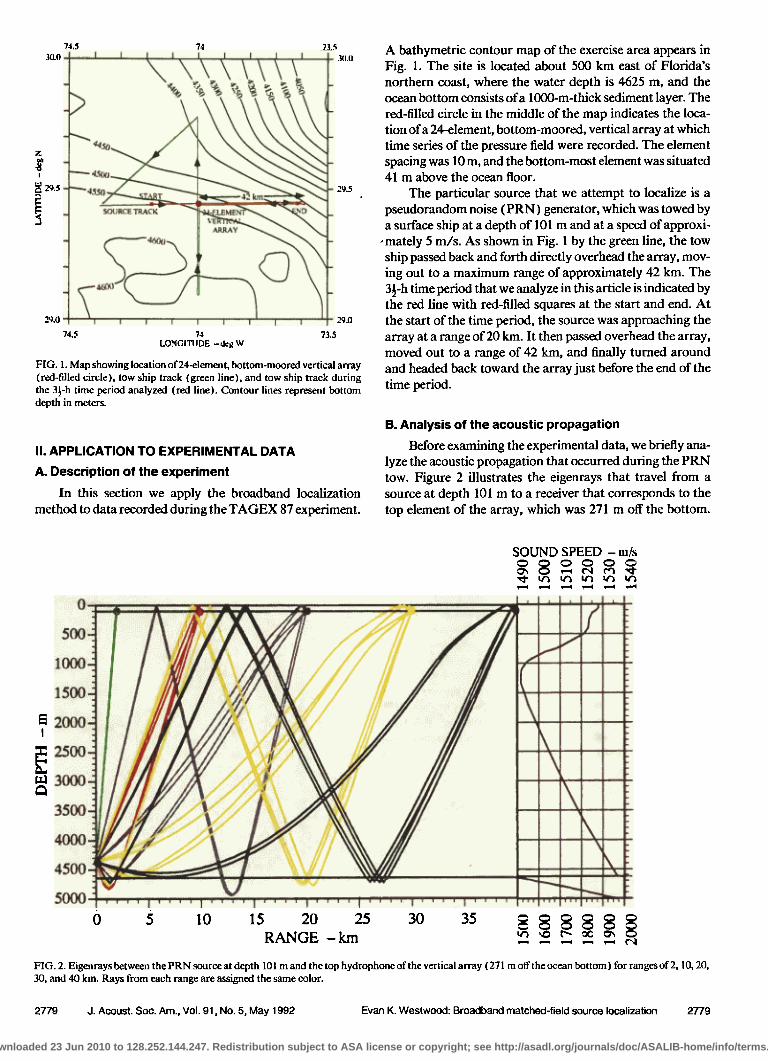
FIG. 1. Map showing location of24-element, bottom-moored vertical array (red-filled circle), tow ship track (green line), and tow ship track during the 3«-h time period analyzed (red line). Contour lines represent bottom depth in meters.

II. APPLICATION TO EXPERIMENTAL DATA

A. Description of the experiment

In this section we apply the broadband localization method to data recorded during the TAGEX 87 experiment.

A bathymetric contour map of the exercise area appears in Fig. 1. The site is located about 500 km east of Florida's northern coast, where the water depth is 4625 m, and the ocean bottom consists ofa 1000-m-thick sediment layer. The red-filled circle in the middle of the map indicates the location of a 24-element, bottom-moored, vertical array at which time series of the pressure field were recorded. The element spacing was 10 m, and the bottom-most element was situated 41 m above the ocean floor.

The particular source that we attempt to localize is a pseudorandom noise (PRN) generator, which was towed by a surface ship at a depth of 101 m and at a speed of approxi-

-mately 5 m/s. As shown in Fig. 1 by the green line, the tow ship passed back and forth directly overhead the array, moving out to a maximum range of approximately 42 km. The 3«-h time period that we analyze in this article is indicated by the red line with red-filled squares at the start and end. At the start of the time period, the source was approaching the array at a range of 20 km. It then passed overhead the array, moved out to a range of 42 kin, and finally turned around and headed back toward the array just before the end of the time period.

B. Analysis of the acoustic propagation

Before examining the experimental data, we briefly analyze the acoustic propagation that occurred during the PRN tow. Figure 2 illustrates the eigenrays that travel from a source at depth 101 m to a receiver that corresponds to the top element of the array, which was 271 m off the bottom.

SOUND SPEED - nt/s

.... I .... I .... I .... I .... [ •'" ' ' I .... I ......... ? ..........

1000-

1500-

2000-

m 3000-

3500-

4000-

4500 -

5O00

0 5 10 15 20 25 30 35 g • g g g • RANGE-krn • • •" •c •,

FIG. 2. Eigenrays between the PRN source at depth 101 m and the top hydrophone of the vertical array (271 m off the ocean bottom) for ranges of 2, 10, 20, 30, and 40 kin. Rays from each range are assigned the same color.

2779 J. Acoust. Sec. Am., Vol. 91, No. 5, May 1992 Evan K. Westwood: Broadband matched-field source localization 2779


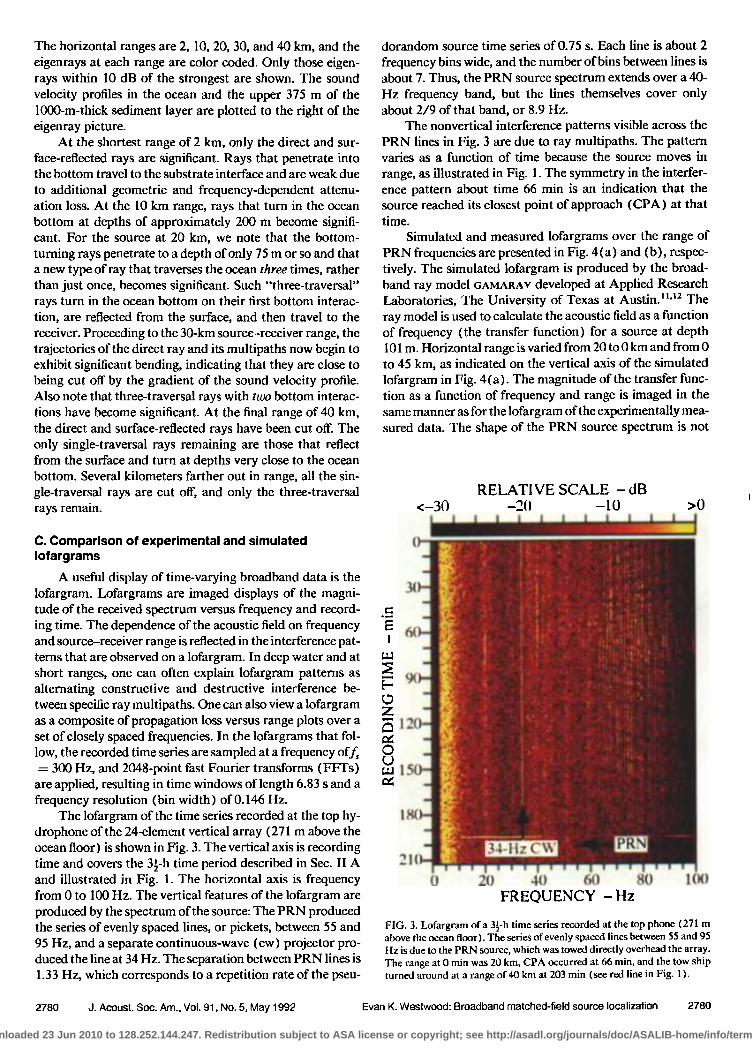
The horizontal ranges are 2, 10, 20, 30, and 40 km, and the eigenrays at each range are color coded. Only those eigenrays within I0 dB of the strongest are shown. The sound velocity profiles in the ocean and the upper 375 m of the 1000-m-thick sediment layer are plotted to the right of the eigenray picture.

At the shortest range of 2 km, only the direct and surface-reflected rays are significant. Rays that penetrate into the bottom travel to the substrate interface and are weak due

to additional geometric and frequency-dependent attenu- ation loss. At the 10 km range, rays that turn in the ocean bottom at depths of approximately 200 m become significant. For the source at 20 km, we note that the bottom- turning rays penetrate to a depth of only 75 m or so and that a new type of ray that traverses the ocean three times, rather than just once, becomes significant. Such "three-traversal" rays turn in the ocean bottom on their first bottom interac- tion, are reflected from the surface, and then travel to the receiver. Proceeding to the 30-km source-receiver range, the trajectories of the direct ray and its multipaths now begin to exhibit significant bending, indicating that they are close to being cut off by the gradient of the sound velocity profile. Also note that three-traversal rays with two bottom interac- tions have become significant. At the final range of 40 km, the direct and surface-reflected rays have been cut off. The only single-traversal rays remaining are those that reflect from the surface and turn at depths very close to the ocean bottom. Several kilometers farther out in range, all the single-traversal rays are cut off, and only the three-traversal rays remain.

dorandom source time series of 0.75 s. Each line is about 2

frequency bins wide, and the number of bins between lines is about 7. Thus, the PRN source spectrum extends over a 40- Hz frequency band, but the lines themselves cover only about 2/9 of that band, or 8.9 Hz.

The nonvertical interference patterns visible across the PRN lines in Fig. 3 are due to ray multipaths. The pattern varies as a function of time because the source moves in

range, as illustrated in Fig. 1. The symmetry in the interference pattern about time 66 rain is an indication that the source reached its closest point of approach (CPA) at that time.

Simulated and measured 1ofargrams over the range of PRN frequencies are presented in Fig. 4(a) and (b), respectively. The simulated 1ofargram is produced by the broadband ray model GAMARAY developed at Applied Research Laboratories, The University of Texas at Austin. ll'•2 The ray model is used to calculate the acoustic field as a function of frequency (the transfer function) for a source at depth 101 m. Horizontal range is varied from 20 to 0 km and from 0 to 45 km, as indicated on the vertical axis of the simulated 1ofargram in Fig. 4(a). The magnitude of the transfer function as a function of frequency and range is imaged in the same manner as for the lofargram of the experimentally measured data. The shape of the PRN source spectrum is not

RELATIVE SCALE - dB <-30 -20 -10 >0

C. Comparison of experimental and simulated Iofargrams

A useful display of time-varying broadband data is the 1ofargram. Lofargrams are imaged displays of the magnitude of the received spectrum versus frequency and recording time. The dependence of the acoustic field on frequency and source-receiver range is reflected in the interference patterns that are observed on a 1ofargram. In deep water and at short ranges, one can often explain lofargram patterns as alternating constructive and destructive interference between specific ray multipaths. One can also view a lofargram as a composite of propagation loss versus range plots over a set of closely spaced frequencies. In the lofargrams that follow, the recorded time series are sampled at a frequency off, ---- 300 Hz, and 2048-point fast Fourier transforms (FFTs) are applied, resulting in time windows of length 6.83 s and a frequency resolution (bin width) of 0.146 Hz.

The 1ofargram of the time series recorded at the top hydrophone of the 24-element vertical array (271 m above the ocean floor) is shown in Fig. 3. The vertical axis is recording time and covers the 37h time period described in Sec. II A and illustrated in Fig. 1. The horizontal axis is frequency from 0 to 100 Hz. The vertical features of the 1ofargram are produced by the spectrum of the source: The PRN produced the series of evenly spaced lines, or pickets, between 55 and 95 Hz, and a separate continuous-wave (cw) projector produced the line at 34 Hz. The separation between PRN lines is 1.33 Hz, which corresponds to a repetition rate of the pseu-

30 : •

E 60 :;' I t

90

120 .,•

150

180

21(I

I I

.',.

,'•., • . PRN 0 21) 40 60 80 I(X)

FREOUENCY - Hz

FIG. 3. Lofargram ofa 3«-h time series recorded at the top phone (271 m above the ocean floor). The series of evenly spaced lines between 55 and 95 Hz is due to the PRN source, which was towed directly overhead the array. The range at 0 min was 20 km, CPA occurred at 66 rain, and the tow ship turned around at a range of 40 km at 203 rain (see red line in Fig. I ).



2(}

10

E

rolo

Z

2O

3O

4O

(a) (b)

I 'l'l I . t

ß I

I

it

'. 0

• ' 30 ! II i

II ,! ..

J I. •j' ß J' B

i

i

l"'J, I .

' I , 150 .!

!

180

J I 60 70 80 90 60 70 80 90

FREQUENCY - Hz FREQUENCY - Hz

210

FIG. 4. Comparison of (a) simulated and (b) experimental Iofargrams at the top phone over the frequency band 55-95 Hz. The broadband ray model used to produce the simulated Iofargram may be used to identify the ray paths that contribute to the interference structure as a function of range. The color scale covers 30 dB in (a) and 20 dB in (b).

included in the simulated 1ofargram in order to show the interference patterns more clearly.

A comparison between the two 1ofargrams in Fig. 4 re- veals considerable similarity. The origin of the changing interference patterns as a function ofrange (time) is explained by the eigenray analysis given in Sec. IIB. The simplest pattern occurs at ranges less than 8 km: A Lloyd's mirror pattern is produced by the direct and surface-reflected rays. The bottom-refracting rays are focused at the receiver when the source is at ranges near 10 kin. Three-traversal rays add to the more complex pattern starting around 15 kin. Between 35 and 40 km the single-traversal rays are gradually cut off, leaving only the three-traversal rays. The good agreement between the 1ofargrams in Fig. 4 indicates that the environ- mental parameters of the experimental area have been well estimated and that the ray model results are accurate.

Before proceeding to the source localization results, we estimate the signal-to-noise ratio (SNR) during the PRN passage by comparing the received level of the source lines with the received level between the source lines (see Fig. 4).

Near CPA and in the center of the 55-95-Hz band, the aver-

age line level is on the order of 17 dB above the average level between lines. When the source is close to 40 km in range (at times 180-200 min), the line level is about 5 dB above the between-line level. To take into account the fact that the

signal only exists over 2/9 of the 55-95-Hz frequency band and thus obtain the average SNR over the band, one would subtract -- 101og,o(2/9) = 6.5 dB from those numbers.

III. RESULTS OF BROADBAND SOURCE

LOCALIZATION

The broadband source localization algorithm described in Sec. I and given by Eqs. (5) and (6) is applied to the same 3•-h time period of the PRN tow described in the previous section and illustrated in Fig. 1. Six of the 24 receivers (numbers 1, 2, 4, 10, 15, and 24, as counted from the bottom of the array u) are used, and coherent summations are made over a frequency band orb = 55-95 Hz. Figure 5 shows the localization as a function of range. (Note that due to the



<-10

3O

6O

90

120

150

RELAT! VE SCALE - dB -8 -6 -4 -2 0

resulting in a total of 342 FFTs during the 3•-h time period. The computation time on a single computational element (CE) of an Alliant FX/8 computer is on the order of 15 min.

The localization of Fig. 5 is successful, as indicated by the generally clear trace that shows the source-receiver range varying as a function of recording time: At time 0 the range is 20 km, the CPA at 0 range occurs at 66 rain, and the maximum range of 42.5 km is attained at 206 min. The localization even reflects the fact that the ship made a 180 • turn at the end of the time period and began to approach the array again.

The localization trace of Fig. 5 is faintest when the source is between 32 and 40 kin. The apparent reason is that over this range interval the single-traversal rays are gradually being cut off (see Sec. IIB), and the signal field becomes weaker than at short ranges (see lofargram in Fig. 4). As a function of array element position, the bottom element loses a given ray first and the top element loses it last. From the time the bottom element loses the ray to the time the top element loses it, the source has traveled about 5 km (note the curvature of the single-traversal rays at range 40 km in Fig.

180

30

210

0 1 (! 2(! 30 40 RANGE - km

FIG. 5. Broadband source localization using Eq. (5) of the 3«-h segment of the PRN tow. The six hydrophones used are numbers I, 2, 4, 10, 15, and 24, as counted from the bottom of the 24-element vertical array. Cross spectra are matched over a frequency band B = 55-95 Hz. The color table shown at the top has a dynamic range of I 0 dB, and values have been normalized such that the maximum in the entire image is 0 dB. The localization indicates that the source started at range 20 kin, passed overhead the array at time 66 rain, and turned around at range 43 km near the end of the time period.

azimuthal symmetry of the array and the assumed environment, no bearing estimate can be obtained.) The color table used to image the localization values is shown at the top of the figure and covers 10 dB. The largest 1ocalizaiton value L [see Eq. (7) ] of the entire image is normalized to 0 dB, and the other values scaled accordingly. The modeled source depth of 101 m is constant. The horizontal axis consists of 151 modeled ranges, from 0 to 45 km in increments of 300 m. The recorded time series are sampled at 300 Hz, and 2048- point FFTs are performed. The processing of the data results in 8 FFTs per minute, but in order to reduce computation time, only one-fifth of the FFTs are used in the localization,

60

9O

120

150

180

210

0 10 20 30 40 RANGE -km

FIG. 6. Localization obtained by normalizing each row separately to have a maximum value of 0 riB.



2). The lack of similar ray arrivals across the vertical extent of the array may contribute to the disruption in localization. Another factor is that the ray model's field computations may not be as accurate at ranges where rays turn at the receiver depth as at other ranges.

Another feature of Fig. 5 is the false localization that occurs at times 170-210 min. The false trace varies from 10

to 15 km, while the true trace varies from 32 to 43 km. The origin of the false localization is that direct rays arriving at the receivers from a source at 10 km produce a nearly identical acoustic field as do the three-traversal rays from a source at 32 km. The similarity in rays can be clearly seen from Fig. 2, in which the red one-traversal rays from I0 km and the yellow three-traversal i'ays from 30 km are almost collocat- ed. (The similarity in fields is also responsible for the weaker false trace at ranges 36-45 km at times 110-120 min, when the source is actually at ranges 12-16 km.) The direct rays that exist at 30 km should make the field distinct from the

field produced by the source at 10 km, but, as explained in the previous paragraph, the direct rays disappear as the

source moves beyond 30 km. One would expect that using hydrophones close to the top of the array might help reduce the false localizations because the direct rays are received at longer ranges.

Figure 6 shows the same localization as in Fig. 5, except that each row of the display has been individually normalized to a maximum of 0 dB. This procedure is equivalent to renormalizing the matched filter output at the end of each recording time period. The result is that the localization trace has been sharpened up at recording times greater than 170 min, when the source range exceeds 32 km. The cost of the sharper "mainlobe" is the rise in the "sidelobes" at other ranges, especially the false localization at ranges between 10 and 15 km. The row normalizatoin procedure may be desir- able in practical applications because it allows the color imaging process to adapt to the weaker localizations one would expect at longer ranges.

The above results indicate that the localization works

well in range. However, we would also like to study how well the algorithm is able to discriminate between submerged

0

(a) (b)

3O

6O

90

120

150

18o

210

0 10 20 30 40 0 1 I! 20 30 40 RANGE - km RPuNG E - km

FIG. 7. Localization obtained when an incorrect source depth of 6 m is used to compute the simulated cross spectra. Compared to the localization that uses the correct depth of I01 m in Fig. 5, the main lobe is less sharp and slightly lower in level, and some sidelobes have increased in level.



sources, such as the 101-m-deep PRN, and surface ships, the effective depth of which is assumed to be 6 m. (Except for slight adjustments in the ray arrival times, the eigenray arrival structure for depth 6 m is basically the same as that shown in Fig. 2 for depth I01 m.) Figure 7 shows localizations of the PRN data that are matched to the incorrect

source depth of 6 m. The image in Fig. 7(a) uses the same normalization and color table as the original 101-m localization of Fig. 5. Although a clear trace is present in Fig. 7(a), the trace is not as bright and sharp as that in Fig. 5, and most of the sidelobes are slightly higher. In particular, the localization trace between 20 and 30 km is considerably weaker. Figure 7 (b) uses the same row normalization procedure as is used in Fig. 6. Again, a clear trace is present, but the trace is noticeably fuzzier, and the sidelobes, especially at short ranges, are higher. In summary, assumption of an incorrect source depth of 6-m results in a false localization of the actual 101-m deep source, but the 6-m localization trace is somewhat inferior to that at 101 m in terms of sharpness and sidelobe level.

IV. FACTORS AFFECTING LOCALIZATION

In this section we examine several factors that affect the success of the broadband source localization. In the localiza-

tions that follow, the correct source depth of 101 m is used to produce the simulated data against which the experimental data are matched. The vertical axes of the localizations run

from the CPA time of 66 rain to the end of the original 3«-h time period, 213 min. The color tables, identical to the one

shown in Fig. 5, cover 10 dB and are normalized so that the maximum in the entire image is 0 dB. Finally, every sixth FFT of the experimental data has been used in the localizations, resulting in 196 data points along the vertical axes.

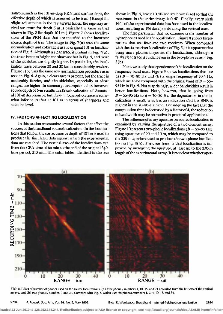
The first parameter that we examine is the number of hydrophones used in the localization. Figure 8 shows localizations that use four and two receivers. When compared with the six-receiver localization of Fig. 5, it is apparent that using more phones improves the localization, although a fairly clear trace is evident even in the two-phone case of Fig. 8(b).

Next, we study the dependence of the localization on the frequency band used. Figure 9 shows localizations that use (a) B = 70-80 Hz and (b) a single frequency of 70.4 Hz, which are to be compared with the original band ofB = 55- 95 Hz in Fig. 5. Not surprisingly, wider bandwidths result in better localizations. Note, however, that in going from B = 55-95 Hz to B = 70-80 Hz, the degradation in the localization is small, which is an indication that the SNR is highest in the 70-80-Hz band. Considering the fact that the computation time is decreased by a factor of 4, the reduction in bandwidth may be attractive in practical applications.

The influence of array aperture on source localization is examined by varying the aperture of a two-element array. Figure 10 presents two-phone localizations (B = 55-95 Hz) using apertures of 90 and I0 m, which may be compared to the 230-m aperture used to produce the two-phone localization in Fig. 8(b). The clear trend is that localization is improved by increasing the aperture, at least up to the 230-m length of the experimental array. It is not clear whether aper-

7O

9O

11o

130

150

170

a b

190

210

0 10 20 30 40 0 10 20 30 40 RANGE - km RANGE -km

FIG. 8. Effect of number of phones used on the source localizations: (a) four phones, numbers 1, 10, 15, and 24 (counted from the bottom of the vertical array), and (b) two phones, numbers 1 and 24. Compare with Fig. 5, which uses six phones, numbers I, 2, 4, 10, 15, and 24.



a 7O

90

• llO

•' 130

Z

• 150

ca 170

190

210 , • •

0 10 20 30 40 0 10 20 30 40 RANGE -km RANGE - km

FIG. 9. Effect of bandwidth on the source localizations for six-phone cases: (a) B = 70-80 Hz, and (b} single frequency of 70.4 Hz. Compare with Fig. 5, which uses B = 55-95 Hz.

tures spanning significant fractions of the water column would further improve the localization, or whether less similar ray paths and loss ofcoherency would degrade the localization.

Finally, we examine factors concerning the broadband source localization algorithm itself. First, the effect of matching the experimental and modeled autospectra, as well as the cross spectra, is considered. The mathematical formu-

9O

110

130

150

170

a b)

190-

210 •

0 10 20 30 40 0 10 20 30 40 RANGE - km RANGE -km

FIG. 10. Effect of aperture on the source localizations for two-phone cases (B = 55-95 Hz): (a} phones 15 and 24 (aperture of 90 m }, and (b} phones I and 2 (aperture of 10 m). Compare with Fig. 8{b}, which uses phones I and 24 (aperture of 230 m).



a 70

90

110

130

150

170

190

210

1

I I I

0 10 20 30 40 0 10 RANGE - km

20 3O 40 RANGE - kin

FIG. 11. Effect of matching the autospectra as well as the cross spectra (equivalent to including the diagonal terms of the matched cross-spectral matrix ): (a) six-phone case (compare to Fig. 5), and (b) two-phone case [compare to Fig. 8(b) ].

la for implementing such an algorithm is the same as that given by Eqs. (5) and (6) except that the second summation in each equation is taken over q = p,N instead of q = p + 1, N. Figure 11 shows localizations that include the autospet-

tra in the matching algorithm for (a) the six-phone case, to be compared with Fig. 5, and (b) the two-phone case, to be compared with Fig. 8(b). Interestingly, the result in both cases is a significant degradation in the localization. In par-

a) (b) 70

90

Ill0

[- 130

Z

• 150

0

m 170

190 - -

210 _

0 10 20 30 40 (! 10 20 30 40 RANGE -km RANGE -km

FIG. 12. Six-phone localization results using all elements of the cross-spectral matrix (equivalent to conventional matched-field processing): (a) Broadband case, B = 55-95 Hz (compare to Fig. 5), and (b) cw case, B ---- 70.4 Hz [compare to Fig. 9(b) ].

2786 d. Acoust. Sec. Am., VoL 91, No. 5, May 1992 Evan K. Westwood: Broadband matched-field source localization 2786


ticular, while the localization trace is still quite clear, the surrounding regions of the image are broadly raised by an average level of 6.7 and 5.3 dB in the six- and two-phone cases, respectively. In addition to the degraded results, inclu- sion of the autospectra terms requires more computation:

The number of phone pairs to match increases from N(N-- 1)/2 to (N-t- 1)N/2, which translates to an increases from 15 to 21 pairs in the six-phone case and from 1 to 3 pairs in the two-phone case.

A second variation on the algorithm that involves use of

7O

90

110

130

Z

•150 o

• 170

b

190

210

0

70

10 20 30 40 RANGE - km

0 10 20 30 40 RANGE - km

90

110

130

15O

170

190

210 ] , • , 0

I m I • I m I J I m I m I

l0 20 30 40 RANGE -km

FIG. 13. Dependence of localization on type of summations used in Eq. (5): (a) incoherent summation over frequency, coherent summation over phone pairs, (b) incoherent summation over phone pairs, coherent summation over frequency, and (c) incoherent summations over both frequency and phone pairs. See Fig. 5 for the results of coherent summation over both frequency and phone pairs.



the autospectra is to perform summations over the entire matched cross-spectral matrix, which, as discussed at the end of Sec. I, is equivalent in the cw case to the linear matched field method. The method involves taking the second summations in both Eqs. (5) and (6) over q = 1, N instead of q = p + 1, N. Moving the summation over the frequency band B in Eq. (5) to the outside and using the fact that the lower triangle of the CSM is the complex conjugate of the upper triangle, the localization quantity for this algorithm may be written

L(,,•= •p_• • Dpq(.l•Mp*q(n)(j• (K(,,,) -• lq=l

= 2 Re[D,, (f)M,,o, , • ] p Iq=p+l

Note that both terms inside the summations of Eq. (9) are real numbers. In contrast, Eq. (5) contains a coherent summation of complex numbers.

Figure 12 shows six-phone localization results using the entire matched CSM for (a) the broadband (B = 55-95 Hz) case, and (b) the cw (B = 70.4 Hz) case. In the broadband case, the results using the entire CSM are significantly more ambiguous than those obtained using the original algorithm (see Fig. 5). In addition, the computation time re- quired to produce Fig. 12(a) was 31 min, compared to 8.5 rain for a comparable localization using the original algorithm. In the narrowband case, however, of Fig. 12(b), the results are somewhat less ambiguous than those obtained using the original algorithm [ see Fig. 9 (b) ]. Two-phone localizations reveal the same interesting pattern: the "matched cross-spectra" method of Eq. (5) is considerably better in the broadband case, but the conventional matched field method is slightly better in the cw case.

The final algorithimic factor we investigate is the method for performing the summations over frequency and phone pairs in Eqs. (5) and (6). In the original algorithm the complex numbers are summed coherently, but an alter- nate method is to take the magnitude of the complex numbers before adding them together. We refer to such a summation as "incoherent" because the phase of the complex numbers is discarded. The following equations are used for (a) incoherent summation over frequency, coherent summation over phone pairs; (b) coherent summation over frequency, incoherent summation over phone pairs, and (c) incoherent summation over frequency, incoherent summation over phone:

p Iq=p+l

(10a)

(•Ob)

1 q=p+ I

(10c)

Figure 13 illustrates the effect of incoherent summation. We observe that the localization using Eq. (10a) in Fig. 13(a) is slightly better than that using Eq. (10b) in Fig. 13 (b), but both are significantly more ambiguous than the totally coherent method [Eq. (5) ] used in Fig. 5. The localization in Fig. 13 (c) using the totally incoherent method of Eq. (10c) exhibits the severest degradation of all the methods. Clearly, the best results are obtained from coherent summations over both frequency and phone pairs.

V. CONCLUSIONS

In this article we have developed a method for broadband source localization and presented results of its application to experimental data. The method is straightforward and easily implemented. It consists of matching measured and modeled cross spectra and coherently adding the "cross- correlated" cross spectra over frequency and hydrophone pairs to obtain the localization quantity. In practical applications, the frequency band over which the summations are performed may be chosen so as to maximize the signal-to- noise ratio.

The source localization method has been applied to an experiment in which a broadband pseudorandom noise generator was towed past a bottom-moored vertical array in deep water. The localization (modeled range versus recording time) using six of the 24 phones and a frequency band of 55-95 Hz exhibited a clear trace that corresponded well to the estimated source track. The depth resolution of the localization method in this particular case is not as good as the range resolution, but a noticeable degradation in the localization is observed when the source depth is modeled as 6 m instead of the correct 101 m.

Not surprisingly, the quality of the source localizations improved as more phones are used, the frequency band over which the cross spectra are matched is increased, and the aperture (in two-phone localizations) is widened. It is also found that coherent summation of the complex numbers over both frequency and phone pairs is superior to incoherent summation.

An interesting and important observation from the experimental localizations is that matching the autospectra in addition to the cross spectra resulted in a significant degradation in the localization. The success of the localization

apparently relies on the coherent addition in the complex plane of the off-diagonal cross-spectral terms. Since the diagonal autospectra terms represent positive real numbers in the complex summation, it appears that they add no infor- mation to the localization and actually serve to overpower the more sensitive off-diagonal terms. Another interesting finding was that in the broadband case our matched cross- spectra method gave better localizations than the straightforward extension of conventional matched-field processing, but in the cw case our method resulted in slightly poorer localizations.

Broadband matched-field processing is an attractive al- ternative to cw processing when the source of interest has broadband components. In order to achieve a given capabili- ty to localize a source, it appears that one may deploy a large array and use a single frequency, or deploy a small array and



use multiple frequencies. The most obvious advantage of the broadband approach is the savings in the hardware cost of additional hydrophones. Another possible advantage is that errors in temporal sampling are usually much less than errors resulting from imperfect knowledge of receiver position. In other words, increasing the bandwidth used in a given matched-field application does not introduce errors because the sampling rate is well known and consistent across hydrophones. In contrast, increasing the number of hydrophones can lead to additional errors due to receiver position uncer- tainty.

This article has presented an extension of the linear matched-field algorithm to the broadband case. We believe that extension of the more complex high-resolution cw matched-field algorithms to broadband applications is a worthwhile area for future research.

ACKNOWLEDGMENTS

This work was supported by Naval Ocean Systems Cen- ter, contract N0039-91-C-0082-1-9-1. The author wishes to thank Dr. Robert A. Koch, Mr. Jonathan Pickett, and Dr. Steven K. Mitchell for their helpful comments and discus- sions regarding this work.

•H. Schmidt, A. B. Baggeroer, W. A. Kuperman, and E. K. Seheer, "Envi- ronmentally tolerant beamforming for high-resolution matched-field pro-

cessing: Deterministic mismatch," $. Acoust. Soc. Am. 88, 1851-1862 (1990).

-•P. M. Velardo, "Robust matched-field source localization," Master's Ihe- sis, Massachusetts Instit ute of Technology (1989).

3A. Parvulescu, "Signal detection in a multipath medium by M.E.S.S. processing," J. Acoust. Soc. Am. 33, 1674 (1961).

SA. Parvulescu and C. S. Clay, "Reproducibility of signal transmissions in the ocean," Radio Eng. Electron. 29, 223-228 (1965).

•C. S. Clay, "Optimum time domain signal transmission and source location in a waveguide," J. Acoust. Soc. Am. 81, 660-664 (1987).

6S. Li and C. S. Clay, "Optimum time domain signal transmission and source location in a waveguide: Experiments in an ideal wedge waveguide," J. Acoust. Soc. Am. 82, 1409-1417 (1987).

?C. S. Clay and S. Li, "Optimum time domain signal transmission and source location in a waveguide: Matched filter and aleconvolution experiments," J. Aeoust. Soc. Am. 83, 1377-1383 (1988).

aW. S. Hodgkiss and R. K. Brienzo, "Broadband source detection and range/depth localization via full-wavefield (matched-field) processing." in Proc. ICASSP-90, 2743-2747 (April 1990).

qL. N. Frazier and P. 1. Pecholcs, "Single-hydrophone localization," J. AcousL Soc. Am. 88, 995-1002 (1990).

ruby "coherent" we mean that the phases of the complex numbers to be summed are not discarded. "Incoherent" summation involves taking the magnitude of the complex numbers before summing.

•E. K. West wood •,nd P. J. Vidmar, "Eigenray finding and time series simulation in a layered-bottom ocean," J. Acoust. Soc. Am. 81, 912-924 ( 1987}.

'•'E. K. Westwood and C. T. Tindie, "Shallow water time series simulation using ray theory," J. Acoust. Soe. Am. 81, 1752-1761 { 1987}.

•Given the 10-m spacing of the original 24-element array, the interelement spacing among the six receivers may be computed as 10, 20, 60, 50, and 90 m.

2789 d. Acoust. Soc. Am., Vol. 91, No. 5, May 1992 Evan K. Westwood: Broadband matched-field source localization 2789


Broadband Matched-field Source Localization

Documents

Transcript of Broadband Matched-field Source Localization