Bristol MSc Time Series Econometrics, Spring 2015

Univariate time series processes, moments, stationarity

Overview

• Moving average processes• Autogregressive processes• MA representation of autoregressive processes• Computing first and second moments, means,

variances, autocovariances, autocorrelations• Stationarity, strong and weak, ergodicity• The lag operator, lag polynomials, invertibility.• Mostly from Hamilton (1994), but see also

Cochrane’s monograph on time series.

Aim

• These univariate concepts needed in multivariate analysis

• Moment calculation a building block in forming the likelihood of time series data, and therefore estimation

• Foundational tools in descriptive time series modelling.

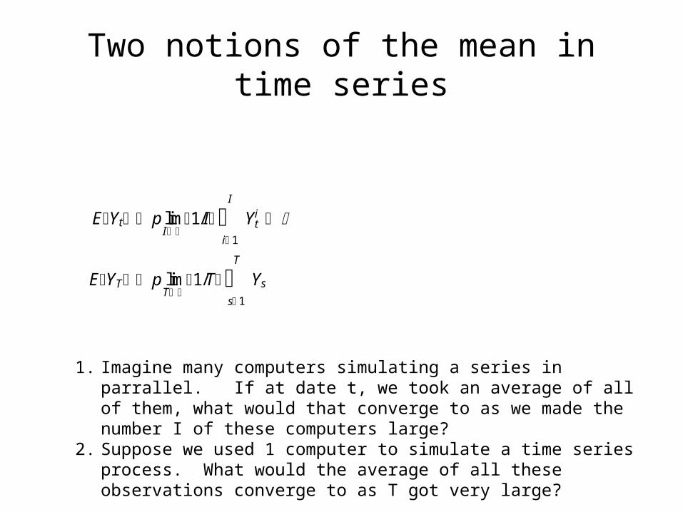
Two notions of the mean in time series

EYt p limI

1/I i 1

I

Yti

EYT p limT

1/T s 1

T

Ys

1. Imagine many computers simulating a series in parrallel. If at date t, we took an average of all of them, what would that converge to as we made the number I of these computers large?

2. Suppose we used 1 computer to simulate a time series process. What would the average of all these observations converge to as T got very large?

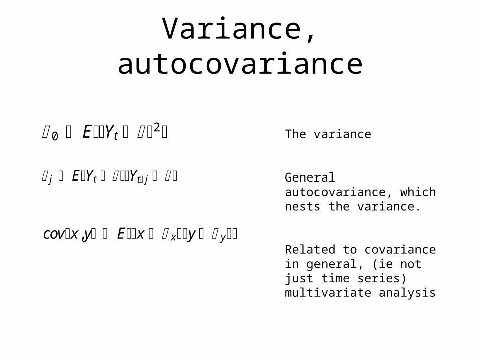
Variance, autocovariance

0 EYt 2

j EYt Yt j

covx,y Ex xy y

The variance

General autocovariance, which nests the variance.

Related to covariance in general, (ie not just time series) multivariate analysis

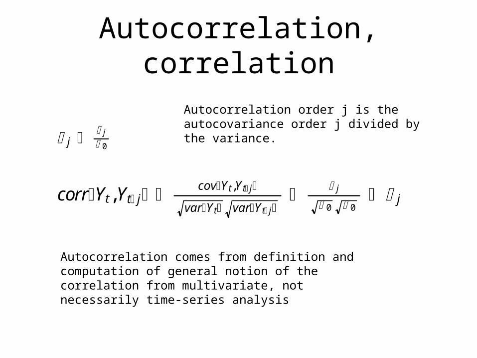
Autocorrelation, correlation

j j 0

corrYt,Yt j covY t,Y t j

varY t varY t j j

0 0 j

Autocorrelation order j is the autocovariance order j divided by the variance.

Autocorrelation comes from definition and computation of general notion of the correlation from multivariate, not necessarily time-series analysis

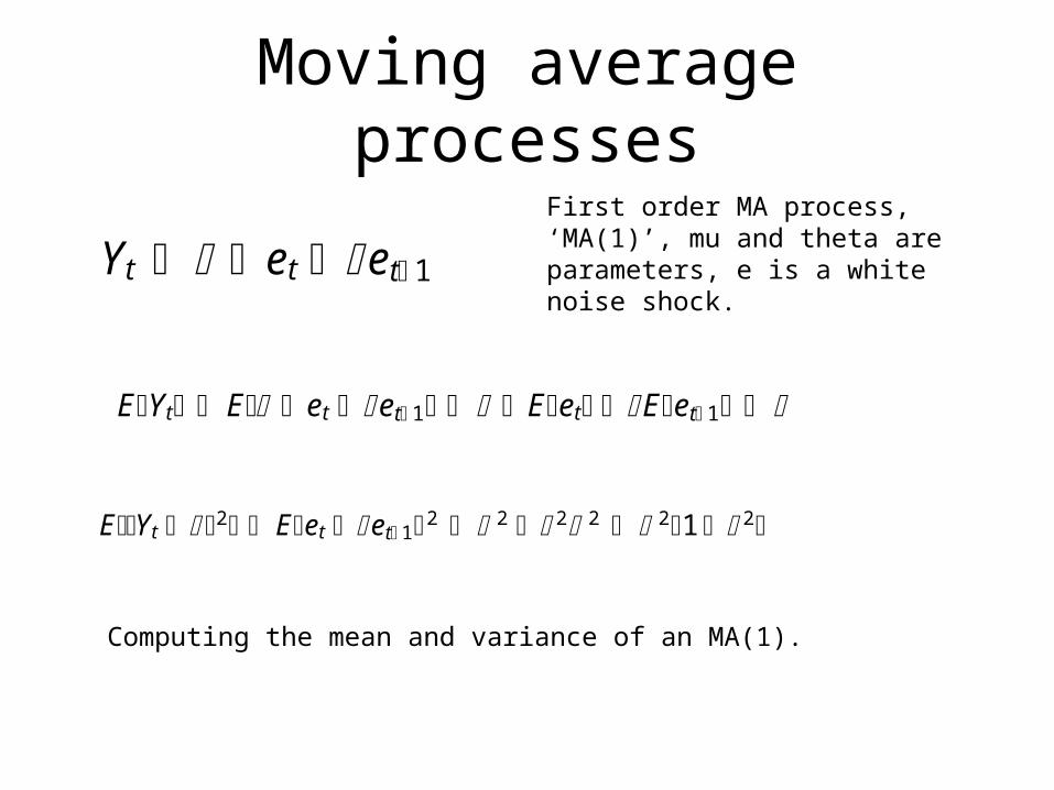
Moving average processes

Yt et et 1

EYt E et et 1 Eet Eet 1

EYt 2 Eet et 12 2 2 2 21 2

First order MA process, ‘MA(1)’, mu and theta are parameters, e is a white noise shock.

Computing the mean and variance of an MA(1).

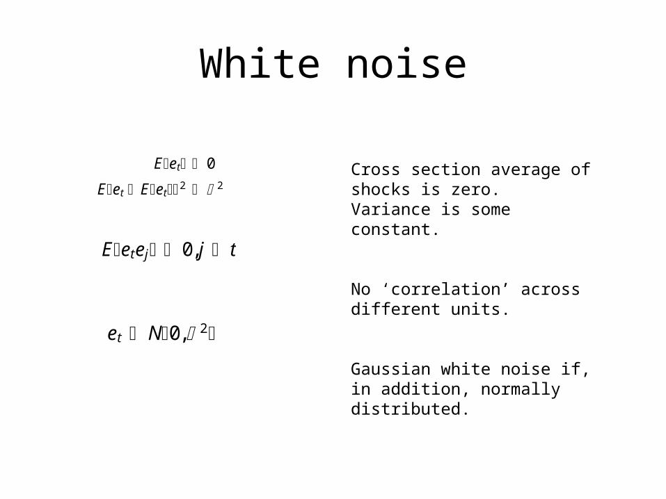
White noise

Eet 0

Eet Eet2 2

Eetej 0, j t

et N0, 2

Cross section average of shocks is zero. Variance is some constant.

No ‘correlation’ across different units.

Gaussian white noise if, in addition, normally distributed.

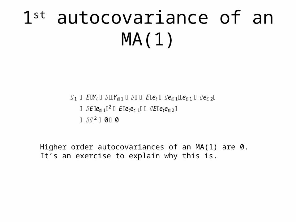
1st autocovariance of an MA(1)

1 EYt Yt 1 Eet et 1et 1 et 2

Eet 12 Eetet 1 Eetet 2

2 0 0

Higher order autocovariances of an MA(1) are 0. It’s an exercise to explain why this is.

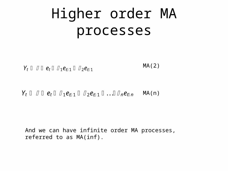
Higher order MA processes

Yt et 1et 1 2et 1

Yt et 1et 1 2et 1 . . . net n

MA(2)

MA(n)

And we can have infinite order MA processes, referred to as MA(inf).

Why ‘moving average’ process?

• The RHS is an ‘average’ [actually a weighted sum]

• And it is a sum whose coverage or window ‘moves’ as the time indicator grows.

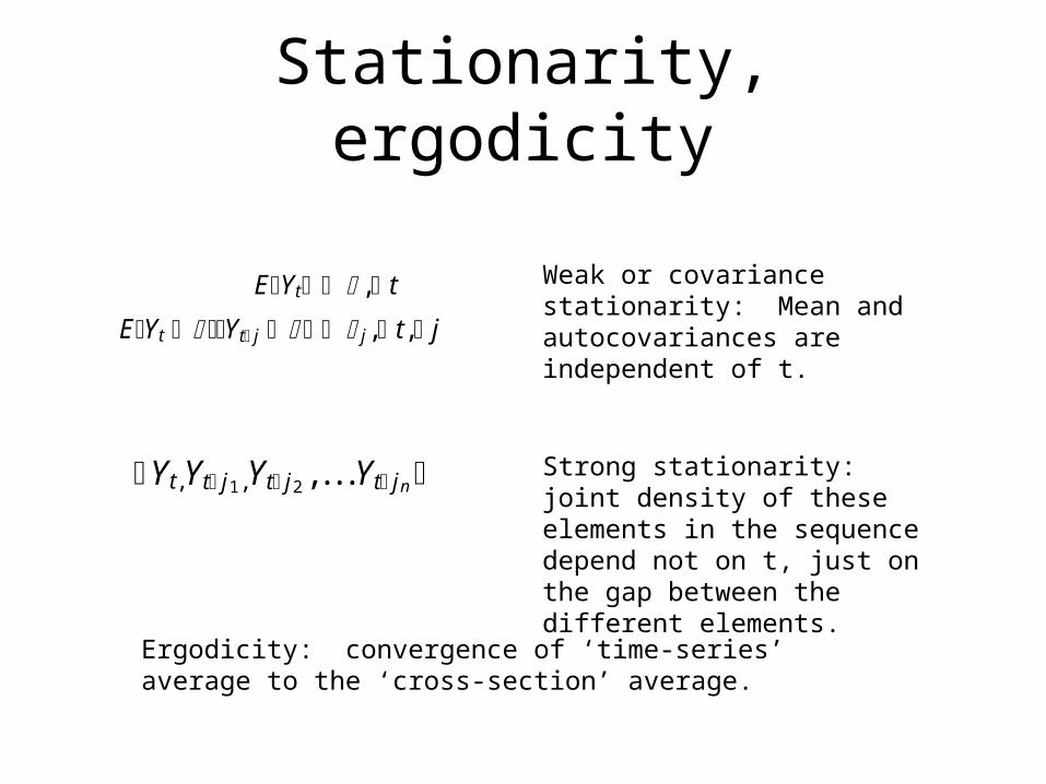
Stationarity, ergodicity

EYt , t

EYt Yt j j, t, j

Weak or covariance stationarity: Mean and autocovariances are independent of t.

Yt,Yt j1,Yt j2 , . . .Yt jn Strong stationarity: joint density of these elements in the sequence depend not on t, just on the gap between the different elements.

Ergodicity: convergence of ‘time-series’ average to the ‘cross-section’ average.

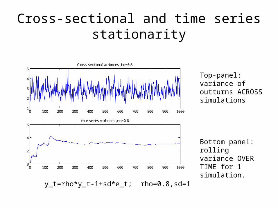
Cross-sectional and time series stationarity

0 100 200 300 400 500 600 700 800 900 10001

2

3

4

5Cross-sectional variances,rho=0.8

0 100 200 300 400 500 600 700 800 900 10000

2

4

6time-series variances,rho=0.8

y_t=rho*y_t-1+sd*e_t; rho=0.8,sd=1

Top-panel: variance of outturns ACROSS simulations

Bottom panel: rolling variance OVER TIME for 1 simulation.

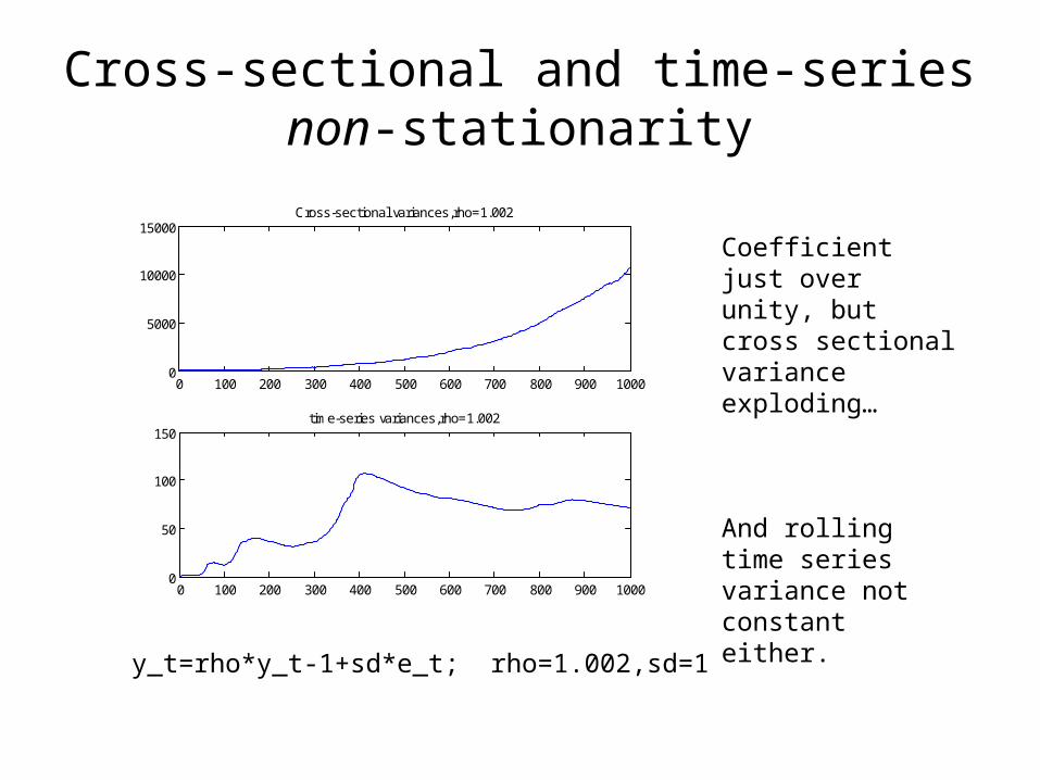
Cross-sectional and time-series non-stationarity

0 100 200 300 400 500 600 700 800 900 10000

5000

10000

15000Cross-sectional variances,rho=1.002

0 100 200 300 400 500 600 700 800 900 10000

50

100

150time-series variances,rho=1.002

y_t=rho*y_t-1+sd*e_t; rho=1.002,sd=1

Coefficient just over unity, but cross sectional variance exploding…

And rolling time series variance not constant either.

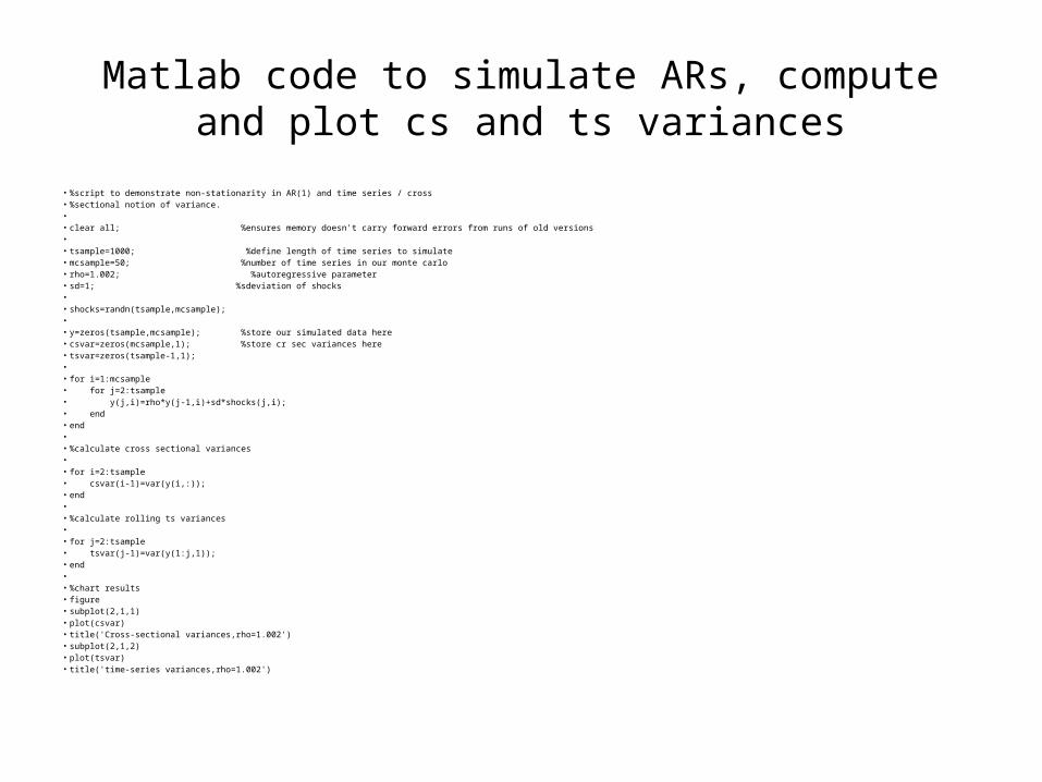
Matlab code to simulate ARs, compute and plot cs and ts variances

• %script to demonstrate non-stationarity in AR(1) and time series / cross• %sectional notion of variance.• • clear all; %ensures memory doesn't carry forward errors from runs of old versions• • tsample=1000; %define length of time series to simulate• mcsample=50; %number of time series in our monte carlo• rho=1.002; %autoregressive parameter• sd=1; %sdeviation of shocks• • shocks=randn(tsample,mcsample);• • y=zeros(tsample,mcsample); %store our simulated data here• csvar=zeros(mcsample,1); %store cr sec variances here• tsvar=zeros(tsample-1,1);• • for i=1:mcsample• for j=2:tsample• y(j,i)=rho*y(j-1,i)+sd*shocks(j,i);• end• end• • %calculate cross sectional variances• • for i=2:tsample• csvar(i-1)=var(y(i,:));• end• • %calculate rolling ts variances• • for j=2:tsample• tsvar(j-1)=var(y(1:j,1));• end• • %chart results• figure• subplot(2,1,1)• plot(csvar)• title('Cross-sectional variances,rho=1.002')• subplot(2,1,2)• plot(tsvar)• title('time-series variances,rho=1.002')

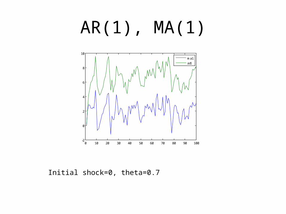
AR(1), MA(1)

0 10 20 30 40 50 60 70 80 90 100-2

0

2

4

6

8

10

ma1

ar1

Initial shock=0, theta=0.7

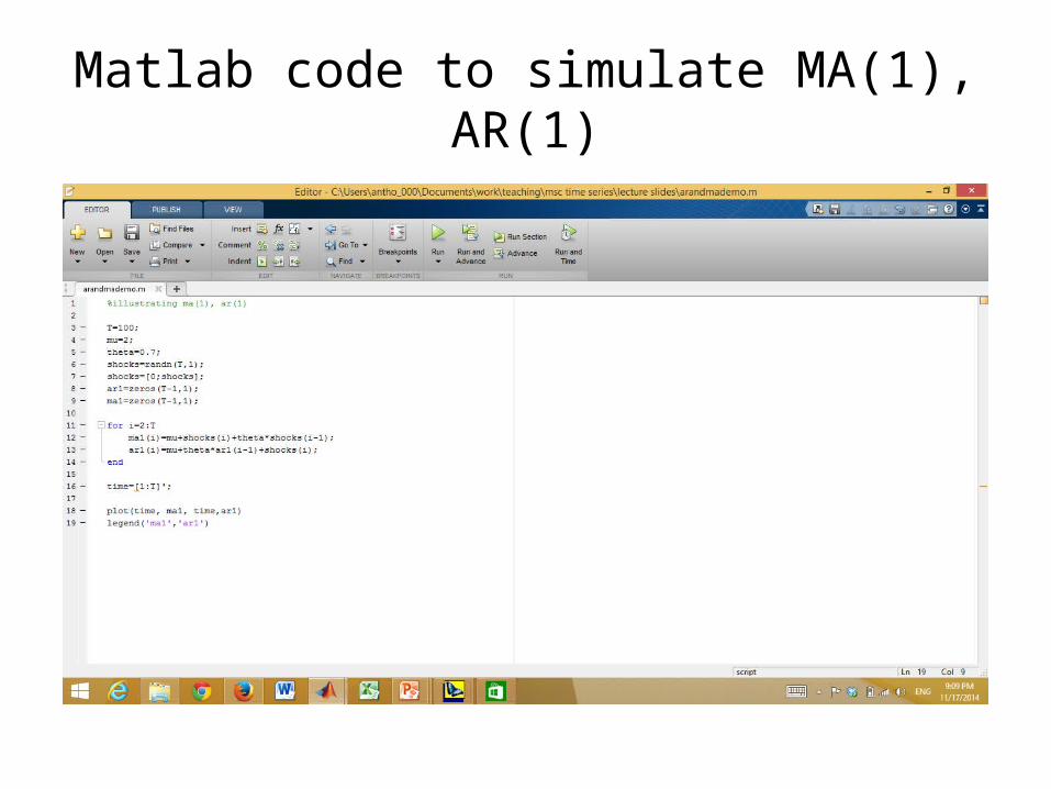
Matlab code to simulate MA(1), AR(1)

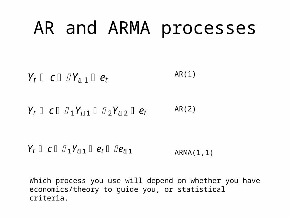
AR and ARMA processes

Yt c Yt 1 et

Yt c 1Yt 1 2Yt 2 et

Yt c 1Yt 1 et et 1

AR(1)

AR(2)

ARMA(1,1)

Which process you use will depend on whether you have economics/theory to guide you, or statistical criteria.

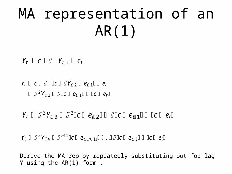
MA representation of an AR(1)

Yt c Yt 1 et

Yt c c Yt 2 et 1 et 2Yt 2 c et 1 c et

Yt 3Yt 3 2c et 2 c et 1 c et

Yt nYt n n 1c et n 1 . . c et 1 c et

Derive the MA rep by repeatedly substituting out for lag Y using the AR(1) form..

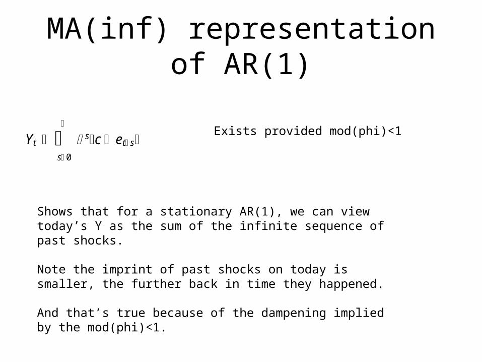
MA(inf) representation of AR(1)

Yt s 0

sc et sExists provided mod(phi)<1

Shows that for a stationary AR(1), we can view today’s Y as the sum of the infinite sequence of past shocks.

Note the imprint of past shocks on today is smaller, the further back in time they happened.

And that’s true because of the dampening implied by the mod(phi)<1.

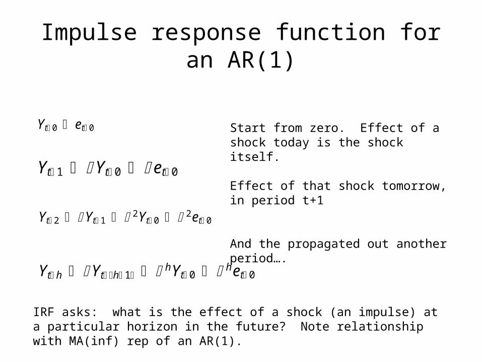
Impulse response function for an AR(1)

Yt 0 et 0

Yt 1 Yt 0 et 0

Yt 2 Yt 1 2Yt 0 2et 0

Yt h Yt h 1 hYt 0 het 0

Start from zero. Effect of a shock today is the shock itself.

Effect of that shock tomorrow, in period t+1

And the propagated out another period….

IRF asks: what is the effect of a shock (an impulse) at a particular horizon in the future? Note relationship with MA(inf) rep of an AR(1).

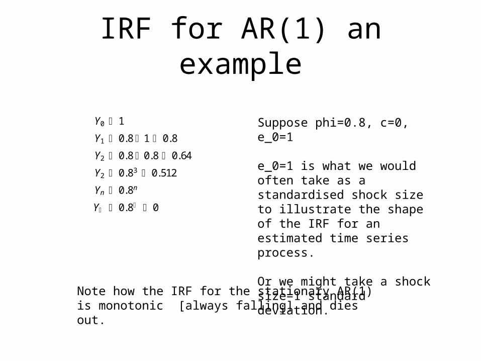
IRF for AR(1) an example

Y0 1

Y1 0.8 1 0.8

Y2 0.8 0.8 0.64

Y2 0.83 0.512

Yn 0.8n

Y 0.8 0

Suppose phi=0.8, c=0, e_0=1

e_0=1 is what we would often take as a standardised shock size to illustrate the shape of the IRF for an estimated time series process.

Or we might take a shock size=1 standard deviation.

Note how the IRF for the stationary AR(1) is monotonic [always falling] and dies out.

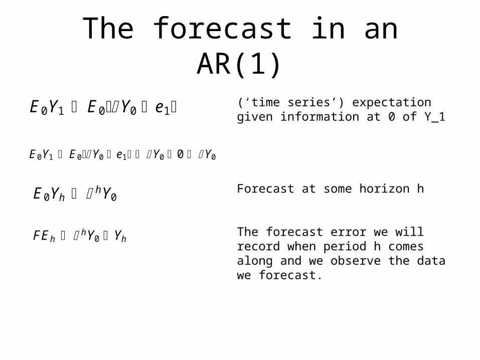
The forecast in an AR(1)

E0Y1 E0 Y0 e1

E0Y1 E0 Y0 e1 Y0 0 Y0

E0Yh hY0

FEh hY0 Yh

(‘time series’) expectation given information at 0 of Y_1

Forecast at some horizon h

The forecast error we will record when period h comes along and we observe the data we forecast.

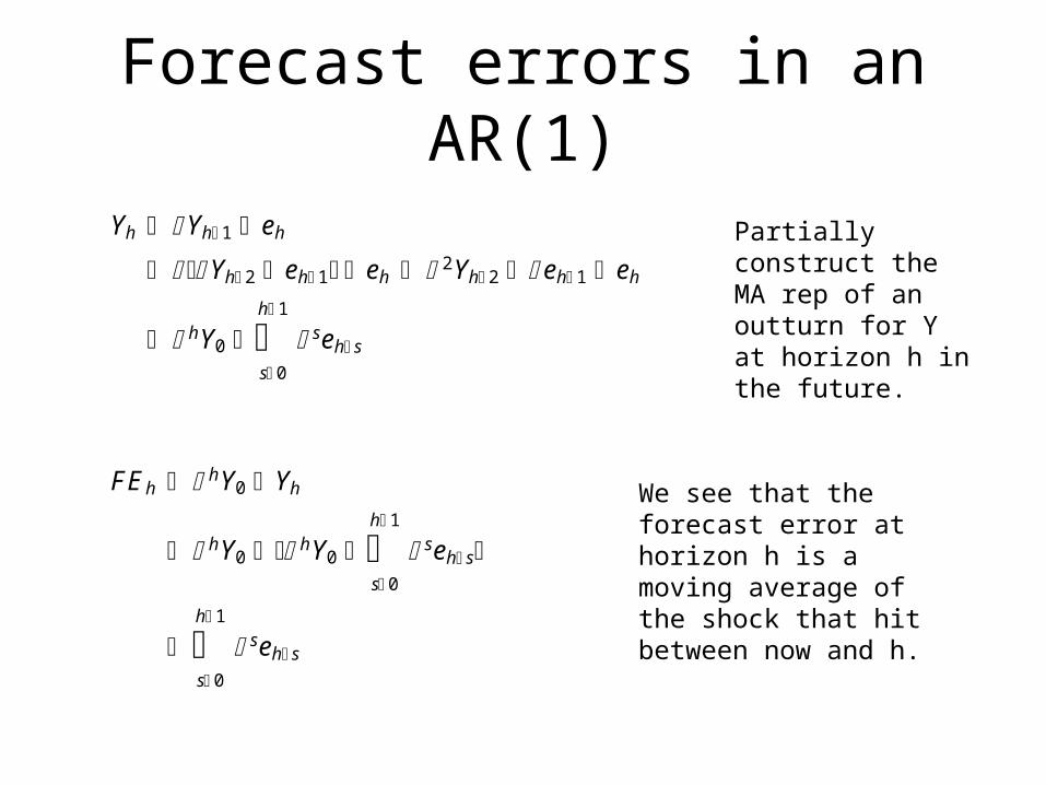
Forecast errors in an AR(1)

Yh Yh 1 eh Yh 2 eh 1 eh 2Yh 2 eh 1 eh

hY0 s 0

h 1

seh s

FEh hY0 Yh

hY0 hY0 s 0

h 1

seh s

s 0

h 1

seh s

Partially construct the MA rep of an outturn for Y at horizon h in the future.

We see that the forecast error at horizon h is a moving average of the shock that hit between now and h.

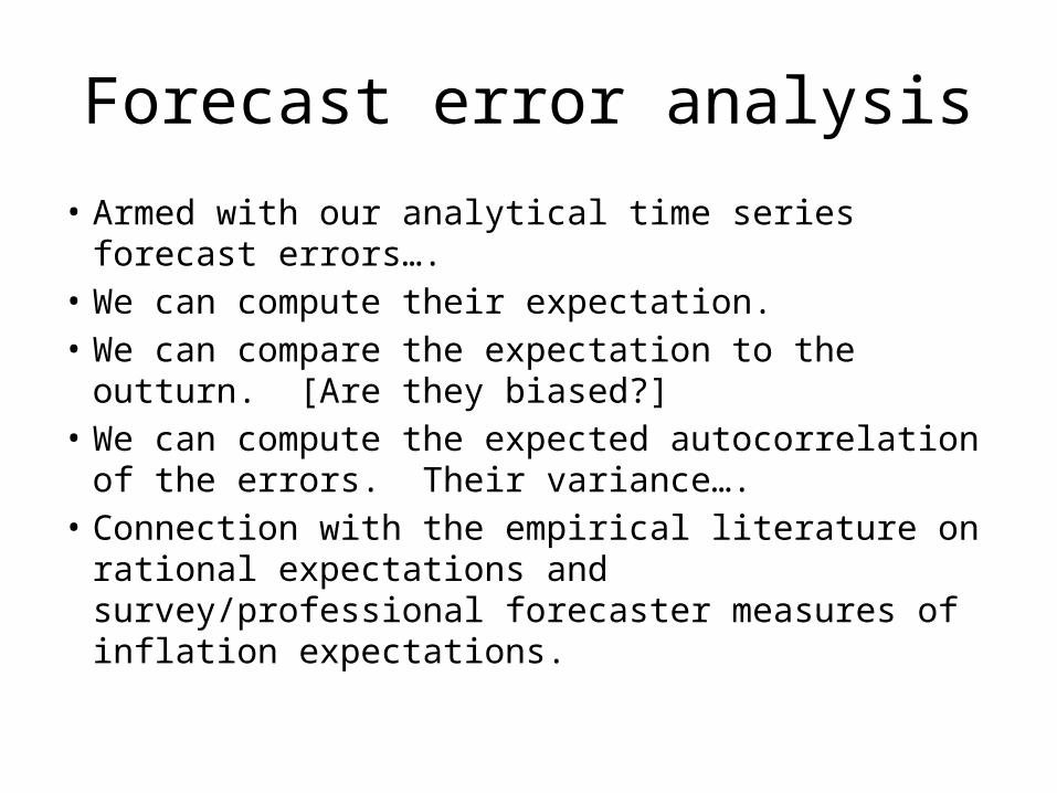
Forecast error analysis

• Armed with our analytical time series forecast errors….

• We can compute their expectation.• We can compare the expectation to the outturn.

[Are they biased?]• We can compute the expected autocorrelation of

the errors. Their variance….• Connection with the empirical literature on rational

expectations and survey/professional forecaster measures of inflation expectations.

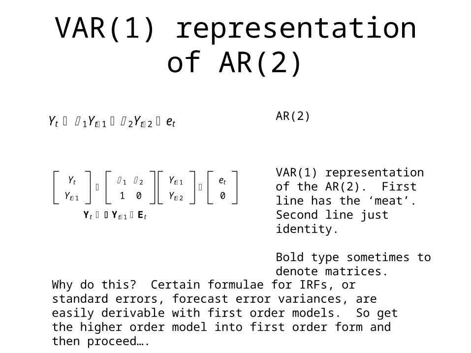
VAR(1) representation of AR(2)

Yt 1Yt 1 2Yt 2 et

Yt

Yt 1

1 21 0

Yt 1

Yt 2

et

0

Yt Yt 1 Et

AR(2)

VAR(1) representation of the AR(2). First line has the ‘meat’. Second line just identity.

Bold type sometimes to denote matrices.

Why do this? Certain formulae for IRFs, or standard errors, forecast error variances, are easily derivable with first order models. So get the higher order model into first order form and then proceed….

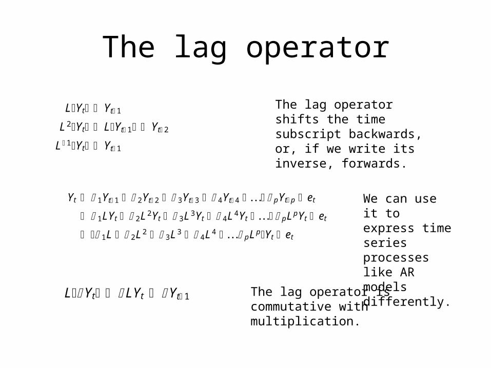
The lag operator

LYt Yt 1L2Yt LYt 1 Yt 2L 1Yt Yt 1

L Yt LYt Yt 1

The lag operator shifts the time subscript backwards, or, if we write its inverse, forwards.

We can use it to express time series processes like AR models differently.

The lag operator is commutative with multiplication.

Yt 1Yt 1 2Yt 2 3Yt 3 4Yt 4 . . . pYt p et

1LYt 2L2Yt 3L3Yt 4L4Yt . . . pLpYt et 1L 2L2 3L3 4L4 . . . pLpYt et

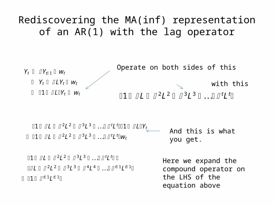
Rediscovering the MA(inf) representation of an AR(1) with the lag operator

Yt Yt 1 w t Yt LYt w t 1 LYt w t 1 L 2L2 3L3 . . . tL t

1 L 2L2 3L3 . . . tL t1 LYt 1 L 2L2 3L3 . . . tL tw t

1 L 2L2 3L3 . . . tL t

L 2L2 3L3 4L4 . . . t 1L t 1

1 t 1L t 1

Operate on both sides of this

with this

And this is what you get.

Here we expand the compound operator on the LHS of the equation above

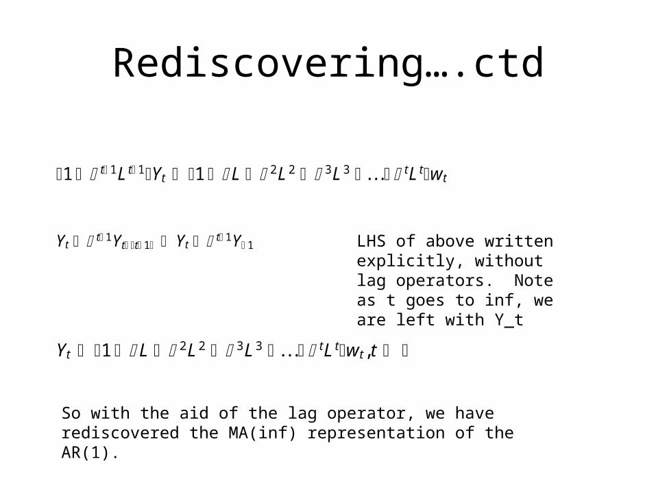
Rediscovering….ctd

1 t 1L t 1Yt 1 L 2L2 3L3 . . . tL tw t

Yt t 1Yt t 1 Yt t 1Y 1 LHS of above written explicitly, without lag operators. Note as t goes to inf, we are left with Y_t

Yt 1 L 2L2 3L3 . . . tL tw t, t

So with the aid of the lag operator, we have rediscovered the MA(inf) representation of the AR(1).

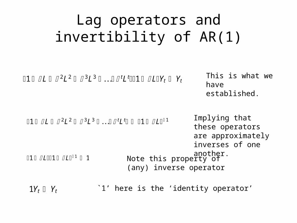
Lag operators and invertibility of AR(1)

1 L 2L2 3L3 . . . tL t1 LYt Yt

1 L 2L2 3L3 . . . tL t 1 L 1

1 L1 L 1 1

1Yt Yt

This is what we have established.

Implying that these operators are approximately inverses of one another.

Note this property of (any) inverse operator

`1’ here is the ‘identity operator’

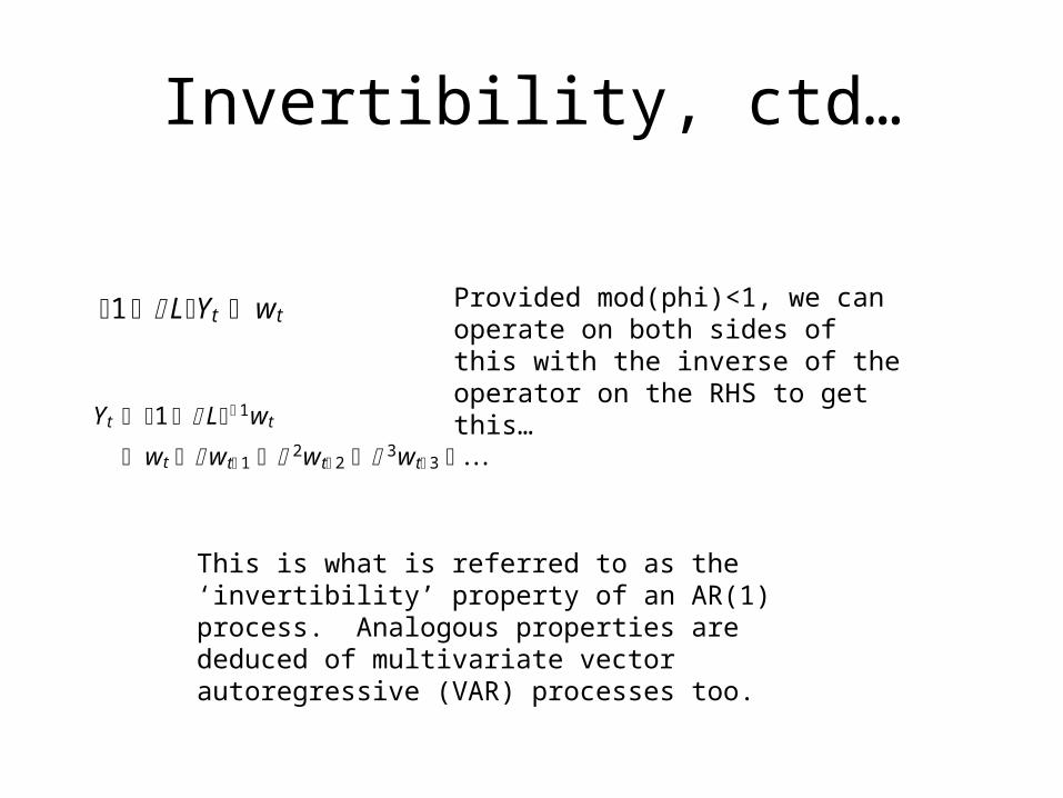
Invertibility, ctd…

1 LYt w t

Yt 1 L 1w t

w t w t 1 2w t 2 3w t 3 . . .

Provided mod(phi)<1, we can operate on both sides of this with the inverse of the operator on the RHS to get this…

This is what is referred to as the ‘invertibility’ property of an AR(1) process. Analogous properties are deduced of multivariate vector autoregressive (VAR) processes too.

Computing mean and variance of AR(2)

• More involved than for the AR(1)• Introduces likelihood computation for more

complex processes• Introduces recursive nature of

autocovariances and its usefulness• NB: it will simply be an exercise to do this for

an AR(1) process.

Mean of an AR(2)

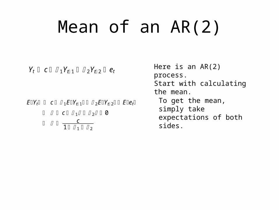
Yt c 1Yt 1 2Yt 2 et

EYt c 1EYt 1 2EYt 2 Eet

c 1 2 0

c1 1 2

Here is an AR(2) process.Start with calculating the mean.

To get the mean, simply take expectations of both sides.

Variance of an AR(2)

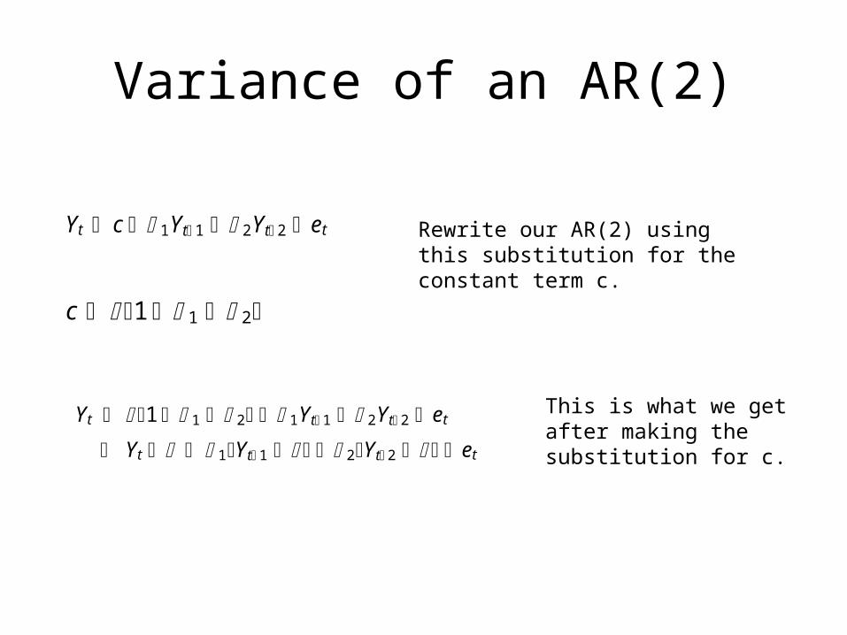
Yt c 1Yt 1 2Yt 2 et

c 1 1 2

Yt 1 1 2 1Yt 1 2Yt 2 et Yt 1Yt 1 2Yt 2 et

Rewrite our AR(2) using this substitution for the constant term c.

This is what we get after making the substitution for c.

Variance of an AR(2)

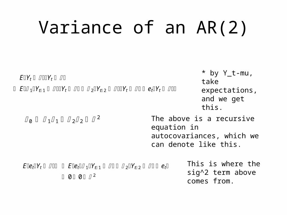
EYt Yt

E 1Yt 1 Yt 2Yt 2 Yt etYt

* by Y_t-mu, take expectations, and we get this.

0 1 1 2 2 2 The above is a recursive equation in autocovariances, which we can denote like this.

EetYt Eet 1Yt 1 2Yt 2 et

0 0 2This is where the sig^2 term above comes from.

Variance of an AR(2)

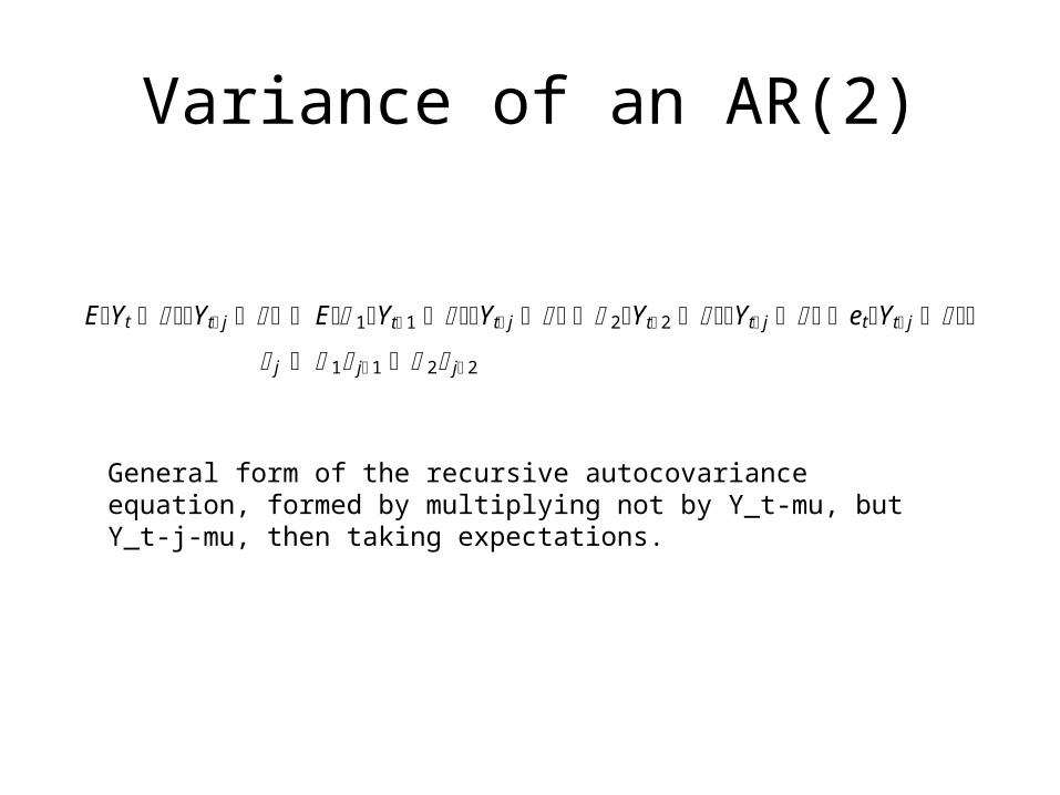
EYt Yt j E 1Yt 1 Yt j 2Yt 2 Yt j etYt j

j 1 j 1 2 j 2

General form of the recursive autocovariance equation, formed by multiplying not by Y_t-mu, but Y_t-j-mu, then taking expectations.

Variance of an AR(2)

j 0 1

j 1 0 2

j 2 0

j 1 j 1 2 j 2

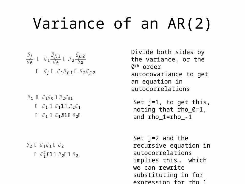
Divide both sides by the variance, or the 0th order autocovariance to get an equation in autocorrelations

1 1 0 2 1

1 11 2 1 1 1 /1 2

Set j=1, to get this, noting that rho_0=1, and rho_1=rho_-1

2 1 1 2 12 /1 2 2

Set j=2 and the recursive equation in autocorrelations implies this… which we can rewrite substituting in for expression for rho_1

Variance of an MA(2)

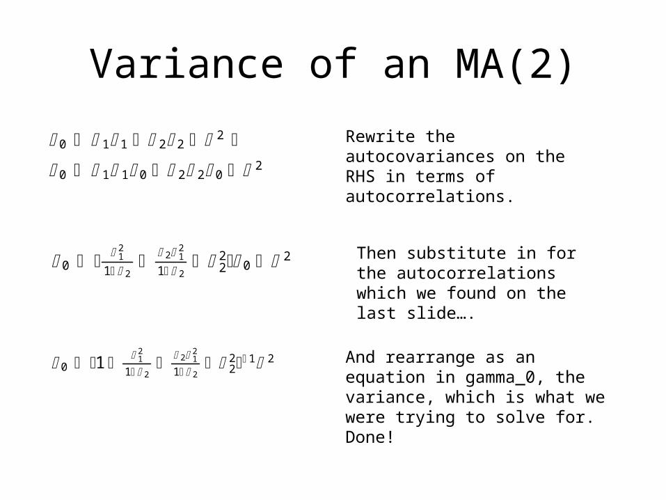
0 1 1 2 2 2

0 1 1 0 2 2 0 2Rewrite the autocovariances on the RHS in terms of autocorrelations.

0 12

1 2 2 1

2

1 2 22 0 2 Then substitute in for the

autocorrelations which we found on the last slide….

0 1 12

1 2 2 1

2

1 2 22 1 2 And rearrange as an equation in

gamma_0, the variance, which is what we were trying to solve for. Done!

Recap

• Moving average processes• Autoregressive processes• ARMA processes• Methods for computing first and second moments

of these• Impulse response• Forecast, forecast errors• MA(infinity) representation of an AR(1)• Lag operators, polynomials in the lag operator