Bright OB stars in the Galaxy - arXivBright OB stars in the Galaxy II. Wind variability in O...
22
arXiv:astro-ph/0505613v1 31 May 2005 Bright OB stars in the Galaxy II. Wind variability in O supergiants as traced by Hα N. Markova 1 , J. Puls 2 , S. Scuderi 3 , and H. Markov 1 1 Institute of Astronomy, Bulgarian National Astronomical Observatory, P.O. Box 136, 4700 Smoljan, Bulgaria e-mail: [email protected] 2 Universit¨ ats-Sternwarte, Scheinerstrasse 1, D-81679 M¨ unchen, Germany e-mail: [email protected] 3 Osservatorio Astrofisico di Catania, Viale A. Doria 6, I-95125, Catania, Italy e-mail: [email protected] Received; Accepted Abstract. In this study we investigate the line-profile variability (lpv) of Hα for a large sample of O-type supergiants (15 objects between O4 and O9.7), in an objective, statistically rigorous manner. We employed the Temporal Variance Spectrum (TVS) analysis, developed by Fullerton, Gies & Bolton (1996) for the case of photospheric absorption lines and modified by us to take into account the effects of wind emission. By means of a comparative analysis we were able to put a number of constraints on the properties of this variability – quantified in terms of a mean and a newly defined fractional amplitude of deviations – as a function of stellar and wind parameters. The results of our analysis show that all the stars in the sample show evidence of significant lpv in Hα , mostly dominated by processes in the wind. The variations occur between zero and 0.3 v∞ (i.e., below ∼ 1.5 R⋆ ), in good agreement with the results from similar studies. A comparison between the observations and corresponding line-profile simulations indicates that for stars with intermediate wind densities the properties of the Hα variability can be explained by simple models, consisting of coherent or broken shells (blobs) uniformly distributed over the wind volume, with an intrinsic scatter in the maximum density contrast of about a factor of two. For stars at lower and higher wind densities, on the other hand, we found certain inconsistencies between the observations and our predictions, most importantly concerning the mean amplitude and the symmetry properties of the TVS. This disagreement might be explained with the presence of coherent large-scale structures (e.g., CIRs), partly confined in a volume close to the star. Interpreted in terms of a variable mass-loss rate, the observed variations of Hα indicate changes of ±4% with respect to the mean value of ˙ M for stars with stronger winds and of ± 16% for stars with weaker winds. The effect of these variations on the corresponding wind momenta is rather insignificant (less than 0.16 dex), increasing only the local scatter without affecting the main concept of the Wind Momentum Luminosity Relationship. Key words. stars: early type – stars: mass loss – stars: winds, outflows – stars: activity – methods: data analysis 1. Introduction The basic philosophy underlying present day hot star model atmospheres contains the assumption of a globally stationary and spherically symmetric stellar wind with a smooth density stratification. Although these models are generally quite successful in describing the overall wind properties, there are theoretical considerations, supported by numerous observational evidences, which indicate that hot stars winds are very far from being smooth and sta- tionary. Send offprint requests to : N. Markova, e-mail: [email protected] The most common approach used to study wind vari- ability in optical and UV domains is to follow line-profile variability (lpv) of one or several spectral lines, formed in different regions, in order to determine relevant time- scales and variability patterns and thus to obtain some insight into the nature and the physical origin of the vari- ations. This kind of surveys requires long sets of stellar spectra with high S/N ratio and high temporal resolu- tion, which implies that only few objects have been in- vestigated so far. Through such investigations clear evi- dence for the presence of large-scale time-dependent wind perturbations (e.g., in the form of Discrete Absorption Components, DACs) was found in UV (Prinja et al. 1992; Massa et al. 1995; Prinja et al. 1996; Kaper et al.
Transcript of Bright OB stars in the Galaxy - arXivBright OB stars in the Galaxy II. Wind variability in O...

arX
iv:a
stro
-ph/
0505
613v
1 3
1 M
ay 2
005
Astronomy & Astrophysics manuscript no. paper June 24, 2018(DOI: will be inserted by hand later)
Bright OB stars in the Galaxy
II. Wind variability in O supergiants as traced by Hα
N. Markova1, J. Puls2, S. Scuderi3, and H. Markov1
1 Institute of Astronomy, Bulgarian National Astronomical Observatory, P.O. Box 136, 4700 Smoljan, Bulgariae-mail: [email protected]
2 Universitats-Sternwarte, Scheinerstrasse 1, D-81679 Munchen, Germanye-mail: [email protected]
3 Osservatorio Astrofisico di Catania, Viale A. Doria 6, I-95125, Catania, Italye-mail: [email protected]
Received; Accepted
Abstract. In this study we investigate the line-profile variability (lpv) of Hα for a large sample of O-type supergiants(15 objects between O4 and O9.7), in an objective, statistically rigorous manner. We employed the TemporalVariance Spectrum (TVS) analysis, developed by Fullerton, Gies & Bolton (1996) for the case of photosphericabsorption lines and modified by us to take into account the effects of wind emission. By means of a comparativeanalysis we were able to put a number of constraints on the properties of this variability – quantified in termsof a mean and a newly defined fractional amplitude of deviations – as a function of stellar and wind parameters.The results of our analysis show that all the stars in the sample show evidence of significant lpv in Hα , mostlydominated by processes in the wind. The variations occur between zero and 0.3 v∞ (i.e., below ∼ 1.5 R⋆ ), in goodagreement with the results from similar studies.A comparison between the observations and corresponding line-profile simulations indicates that for stars withintermediate wind densities the properties of the Hα variability can be explained by simple models, consistingof coherent or broken shells (blobs) uniformly distributed over the wind volume, with an intrinsic scatter in themaximum density contrast of about a factor of two. For stars at lower and higher wind densities, on the otherhand, we found certain inconsistencies between the observations and our predictions, most importantly concerningthe mean amplitude and the symmetry properties of the TVS. This disagreement might be explained with thepresence of coherent large-scale structures (e.g., CIRs), partly confined in a volume close to the star.Interpreted in terms of a variable mass-loss rate, the observed variations of Hα indicate changes of ±4% withrespect to the mean value of M for stars with stronger winds and of ± 16% for stars with weaker winds. The effectof these variations on the corresponding wind momenta is rather insignificant (less than 0.16 dex), increasing onlythe local scatter without affecting the main concept of the Wind Momentum Luminosity Relationship.
Key words. stars: early type – stars: mass loss – stars: winds, outflows – stars: activity – methods: data analysis
1. Introduction
The basic philosophy underlying present day hot starmodel atmospheres contains the assumption of a globallystationary and spherically symmetric stellar wind with asmooth density stratification. Although these models aregenerally quite successful in describing the overall windproperties, there are theoretical considerations, supportedby numerous observational evidences, which indicate thathot stars winds are very far from being smooth and sta-tionary.
Send offprint requests to: N. Markova,e-mail: [email protected]
The most common approach used to study wind vari-ability in optical and UV domains is to follow line-profilevariability (lpv) of one or several spectral lines, formedin different regions, in order to determine relevant time-scales and variability patterns and thus to obtain someinsight into the nature and the physical origin of the vari-ations. This kind of surveys requires long sets of stellarspectra with high S/N ratio and high temporal resolu-tion, which implies that only few objects have been in-vestigated so far. Through such investigations clear evi-dence for the presence of large-scale time-dependent windperturbations (e.g., in the form of Discrete AbsorptionComponents, DACs) was found in UV (Prinja et al.1992; Massa et al. 1995; Prinja et al. 1996; Kaper et al.

2 Markova et al.: Wind variability in O stars
1999; Prinja et al. 2002) and optical (Fullerton et al. 1992;Prinja & Fullerton 1994; Rauw et al. 2001; Prinja et al.2001; Markova 2002) spectra of many O and early Bstars. Since DACs have been observed in WR stars(Prinja & Smith 1992) and in an LBV (Markova 1986)as well, they are thought to be a fundamental property ofradiative driven stellar winds.
Another source of lpv in hot stars winds aresmall-scale structures (clumps) which are believedto result from strong instabilities in the wind it-self (Owocki, Castor & Rybicki 1988; Feldmeier 1995;Owocki & Puls 1999). While the clumped nature of WRwinds was unambiguously proven by observations, thepresence of clumps in O-star winds has so far re-lied on indirect evidence only (Crowther et al. 2002;Bianchi & Garcia 2002; Markova et al. 2004).
Wind structures and temporal variability are amongthe most important physical processes that may sig-nificantly modify the mass loss rates derived fromobservations. Since accurate mass loss rates are cru-cial for evolutionary studies (e.g., Meynet et al. 1994)and for extra-galactic distance determinations (via theWind Momentum Luminosity Relationship (WLR), cf.Kudritzki & Puls 2000), it is particularly important toknow to what extent the outcome of these studies mightbe influenced by uncertainties in M due to the effects ofwind structures and variability. Indeed, Kudritzki (1999)has noted that wind variability is not expected to affectthe concept of the WLR significantly. However, this sug-gestion is based on results obtained via a detailed investi-gation of one object alone, while similar data for a largenumber of stars of different spectral types and luminosityclasses are needed to resolve the problem adequately.
Following the outlined reasoning, a project to studythe effects of wind structure and variability in Galactic O-type stars has been recently started by our group. Whilein a previous paper (Markova et al. 2004, Paper I) we havedealt with problems concerning the WLR and the effects ofwind clumping, in the present one we address the questionof wind variability as traced by Hα and the dependence (ifany) of the properties of this variability on fundamentalstellar and wind parameters. In particular, in Sect. 2 wedescribe the observational material and its reduction. InSect. 3 we outline the method used to detect and analyzethe Hα lpv. In Sect. 4, 5 and 7 the results of our analy-sis are presented in detail while in Sect. 6 the outcomesof some simple 1- and 2-D simulations are described. InSect. 8 we summarize the major results and give somecomments and conclusions.
2. Observations and data reduction
Our sample consists of 15 Galactic supergiants with spec-tral classes from O4 to O9.7, all drawn from the list ofstars analyzed by Markova et al. (2004) in terms of theirmass-loss and wind momentum rates. Table 1 lists theobjects along with some of their stellar and wind parame-
ters, as used in the present study. All data are taken fromPaper I.
A total of 82 high-quality Hα spectra (R =15 000) of the sample stars were collected between1997 and 1999. The observations were obtained atthe Coude focus of the 2m RCC telescope atthe National Astronomical Observatory (Bulgaria) us-ing an ELECTRON CCD (520×580,22×24µ) and aPHOTOMETRIC CCD (1024×1024,24µ).1 For all starsbut one the S/N ratio, averaged within each spectraltime series, lies between 150 to 250, while in the case ofHD 190429 it is ∼100.
The temporal sampling of the data for each target isnot systematic but random, with typical values of theminimum and maximum time intervals between succes-sive spectra of 1 to 2 and 7 to 8 months, respectively. Inseveral cases observations with a time-resolution of 1 to 5days are also available, but in none of these cases these ob-servations dominate the corresponding time series. Thus,we expect the results of our survey to be sensitive to vari-ations which occur on a time-scale which is significantlylarger than the corresponding wind flow time (of the orderof a couple of hours).
More information about the observational materialand its reduction can be found in Markova & Valchev(2000) and in Paper I. In particular, to reduce the obser-vations we have followed a standard procedure (developedin IDL) which includes: bias subtraction, flat-fielding, cos-mic ray hits removal, wavelength calibration, correctionfor heliocentric radial velocity, water vapor lines removaland re-binning to a step size of 0.2 A per pixel.
3. Methodology and measurements
Since we were going to study a large number of objectsand since in many cases our observations were not sys-tematic but with large temporal gaps in between, fromthe onset of this investigation on we recognized that ourability to characterize the wind variability of individualtargets would be restricted, e.g., we would not be able todetermine time-scales and variability patterns. Moreover,to work effectively, we would need to employ some simpleand fast method both to detect and quantify lpv and toconstrain the properties of this variability as a functionof fundamental stellar and wind parameters of the samplestars.
Fullerton, Gies & Bolton (1996) have developed a verysensitive and rigorous method to handle lpv that is poorlysampled in time. This method, called Temporal VarianceSpectrum (TVS) analysis, was proven to be a powerfultool to detect and compare lpv of pure absorption profiles.
1 The use of different detectors is not expected to bias thehomogeneity of our sample because the noise characteristicsof these two devices are practically the same. The root-mean-square (rms) read-out noise of the ELECTRON CCD is 3 elec-trons per pixel (i.e 1.5 ADU with 2 electrons per ADU) whilethe rms read-out noise of the PHOTOMETRIC CCD is 3.3electrons per pixel (2.7 ADU with 1.21 electrons per ADU).

Markova et al.: Wind variability in O stars 3
Table 1. Stellar and wind parameters of the sample stars used in the present study. All data are taken fromMarkova et al. (2004).
Object Sp vsys Teff R⋆ log g YHe logL v sin i v∞ β
HD 190 429A O4If+ -36 39 200 20.8 3.65 0.14 5.97 135 2 400 0.95HD 16 691 O4If -51 39 200 19.8 3.65 0.10 5.92 140 2 300 0.96HD 14 947 O5If -56 37 700 25.6 3.56 0.20 6.08 133 2 300 0.98HD 210 839 O6If -71 36 200 23.0 3.48 0.10 5.91 214 2 200 1.00HD 192 639 O7Ib(f) -7 34 700 17.2 3.39 0.20 5.59 110 2 150 1.09HD 17 603 O7.5Ib(f) -40 34 000 25.2 3.35 0.12 5.88 110 1 900 1.05HD 24 912 O7.5I(f) 59 34 000 25.2 3.35 0.15 5.88 204 2 400 0.78HD 225 160 O8Ib(f) -40 33 000 22.4 3.31 0.12 5.73 125 1 600 0.85HD 338 926 O8.5Ib -9 32 500 22.7 3.27 0.12 5.72 80 2 000 1.00HD 210 809 O9Iab -90 31 700 19.6 3.23 0.14 5.54 100 2 100 0.91HD 188 209 O9.5Iab -16 31 000 19.6 3.19 0.12 5.51 87 1 650 0.90BD+56 739 O9.5Ib -5 31 000 19.6 3.19 0.12 5.51 80 2 000 0.85HD 209 975 O9.5Ib -18 31 000 19.2 3.19 0.10 5.49 90 2 050 0.80HD 218 915 O9.5Iab -84 31 000 19.6 3.19 0.12 5.51 80 2 000 0.95HD 18 409 O9.7Ib -51 30 600 15.7 3.17 0.14 5.29 110 1 750 0.70
However, its potential with respect to profiles influencedby wind emission has not been tested systematically so far.Although the application of the TVS technique to detectlpv in emission lines does not seem to pose serious prob-lems (e.g., Kaufer et al. 1996; Kaper et al. 1997; Markova2002), its implication for the objectives of a comparativeanalysis (e.g. to compare the strength of lpv in differentlines or different stars) certainly needs to be carefully in-vestigated.
To study the Hα variability of the stars in our samplewe modified the main philosophy of the TVS analysis inorder to take into account the effect of wind emission.
To compute the TV S of Hα as a function of veloc-ity across the line and to determine the velocity widthover which significant variability occurs, ∆V , we followedFullerton, Gies & Bolton (1996) but assumed that thenoise is dominated by photon noise.2 In this case, the TV Sfor the pixels in column j (i.e., at wavelength/velocity j)is calculated from
TV Sj =
N∑
i
w(i)(Sij − Sj)2
Sij(N − 1)(1)
where Sj is the weighted mean spectrum for the j-th pixel,averaged over a time series of N spectra, and given by
Sj =
∑Ni Sijwi
N. (2)
with the weighting factors, wi, given by
wi =( σ0
σic
)2(3)
where
σ0 =
(
1
N
N∑
i
σ−2ic
)−1
(4)
2 This assumption seems to be justified because we rely onCoude spectra of relatively high quality.
and σic is the value of the noise in the i-th spectrum,averaged over a certain number of continuum pixels (40in our case).
The RMS deviations (RMS = TV S0.5) as a functionof velocity across Hα for the time series of each target areshown in the top panels of Figures 1 to 3. The level of de-viations in the continuum, σ0, is represented by a dashedline, while the threshold of significant lpv, fixed at thecorresponding 99% confidence level of the σ2
0χ2N−1 distri-
bution, is marked with a dashed-dotted line. We want tostress here that although our implementation is in terms ofTV S0.5, hereafter we shall continue to refer to the “TVS”and the “TVS analysis”, respectively.3
To localize the Hα lpv in velocity space we used the“blue” and “red” velocity limits of significant variability,vb and vr, introduced by Fullerton, Gies & Bolton (1996).The measurements have been performed interactively tofix the positions of the two points where the TVS crossesthe horizontal line representing the threshold of significantlpv. The accuracy of these measurements depends on thequality of the data used and on the strength of lpv. Forexample, in the limiting case of a strong lpv (i.e., a TVSwith large amplitudes and steep spectral gradients) the ac-curacy of the individual measurements might be as goodas ±20 km s−1 . Alternatively, in the case of a weak lpv(e.g., with amplitudes just above the threshold of signif-icant variability) the determination of the velocity limitsmight become so uncertain that different positions of al-most similar probability may exist for each limit. In theselatter cases and in order to assess the effects of such un-certainties on the outcomes of our analysis, we provide
3 Root mean square deviations have been used instead ofthe TVS itself since the former quantity scales linearly withthe size of the deviations. Thus, it is more appropriate for adirect comparison of the strength of lpv in various stars (seealso Fullerton et al.).

4 Markova et al.: Wind variability in O stars
two couples of estimates for vb and vr. These two sets ofvalues, expressed in km s−1 , are listed in Column 6 ofTable 2 as a first and a second entry. We consider the firstentry as the more reliable one and will refer to it as the“conservative case”.
As a by-product of the measurement of vb and vr, weobtain the total velocity width over which significant vari-ability in Hα occurs, ∆V = (vr − vb). In order to findsome constraints on the distribution of the lpv in physi-cal space, we furthermore determined the radial distancermax, where v(r = rmax) = vb, assuming that the windvelocity obeys a standard law of the form
v(r) = v∞(
1− bR⋆
r
)β, (5)
b = 1−(vmin
v∞
)1/β, (6)
with β and v∞ from Table 1 and vmin = 1.0 km s−1 . Theobtained estimates of rmax, expressed in units of R⋆ , aregiven in Column 7 of Table 2. We are aware of the factthat emission variability is difficult to localize and couldin principle be due to the net effect of fluctuations thatoccur in different locations under different conditions andtherefore consider these estimates as upper limits only.
To quantify and compare lpv,Fullerton, Gies & Bolton (1996) have introduced twoparameters, called mean and fractional amplitude ofdeviations, Alpv and alpv. In the following we will referto these quantities as to AF and aF (with “F” referringto Fullerton). The first parameter is expressed in unitsof the normalized continuum flux, while the second oneis a dimensionless quantity. The authors define thesequantities as follows:
AF =1
∆V
∫ vr
vb
TV S0.5j dv (7)
aF =100
∫ vrvb
(
TV Sj − σ20
)0.5dv
∫ vrvb
∣
∣Sj − 1∣
∣ dv(8)
The above expressions imply the following. First, themean amplitude of deviations is independent of profiletype and thus can be used for evaluating the statisticalsignificance of lpv both in absorption and in emission pro-files. Second, the fractional amplitude depends (via thedenominator) on the strength of the underlying spectralfeature but does not make any difference between profilesin absorption and in emission. Particularly, it becomes anon-monotonic function of wind strength, with a maxi-mum in those regions where the wind-emission has (moreor less) completely filled in the photospheric absorption,i.e., where the net equivalent width within [vb, vr] is closeto zero. Therefore, this quantity is inappropriate for inves-tigating profiles which are influenced by wind emission ofdifferent extent. Actually, this problem has already beenoutlined by Fullerton et al.
In order to optimize the fractional amplitude to ac-count for the systematic difference in the strength of
Hα as a function of wind strength, we decided to nor-malize the integral over the TVS to a quantity which wecalled “Fractional Emission Equivalent Width” (FEEW).With this new definition of the fractional amplitude, nowdenoted by aN to distinguish it from Fullerton’s parame-ter aF, this quantity is a measure of the observed degree ofvariability per unit fractional wind emission. “Fractional”refers here to the observed range of significant variability,[vb, vr]. Formally, aN is given by4
aN =100
∫ vrvb
(
TV Sj − σ20
)0.5dv
∫ vrvb
(
Sj − 1)
dv −∫ vrvb
(Sphotj − 1) dv
(9)
The first term in the denominator of Eq.9 represents thefractional equivalent width of the observed profile (posi-tive for emission and negative for absorption), while thesecond one gives the fractional equivalent width of thephotospheric component of Hα (always negative). In total,the denominator thus gives the fractional wind emission(always positive). A further discussion of aN is given inSect. 6.
The mean amplitude, as defined by Eq. 7, on the otherhand, does not seem to pose any problem concerning anassessement of the statistical significance of variabilityacross Hα. In their original study, Fullerton et al. havenoted that this quantity cannot serve as a comparativetool because it does not account for differences in thestrength of the underlaying absorption feature. In con-trast, in the case of Hα from O-type supergiants the meanamplitude might depend on the wind strength5 and mighttherefore become of interest as well, in order to examineand to compare the wind variability in stars of variousspectral types. Motivated by this possibility we re-definedthe mean amplitude to account (partially) for differencesin the overall quality (i.e., in S/N) of the time series of thesample stars, by subtracting σ2
0 from the TVS,
AN =100
∆V
∫ vr
vb
(
TV Sj − σ20
)0.5dv. (10)
The photospheric profiles of Hα required to derive the val-ues of aN have been selected from a grid of plane-parallelmodels in dependence of the particular stellar parameters(Table 1, see also Paper I). Note that the (relative) uncer-tainty of the denominator becomes rather large in thosecases where the wind-emission is only marginal, since inthis case the errors introduced by uncertainties in the stel-lar parameters (affecting the actual choice of the photo-spheric profiles) become significant.
To estimate the uncertainty in aN we followedFullerton, Gies & Bolton (1996) but used a re-formulation(derived by A. Fullerton, priv. com.) of their Eq. 16.
4 In this expression, we have accounted only for uncertaintiescaused by photon noise while the error due to small differencesin the continuum level of individual spectra in a given timeseries is neglected.
5 E.g., the numerator in Eq. 7 is expected to react on winddensity (the higher the density the larger the emitting volume).

Markova et al.: Wind variability in O stars 5
Additionally, we assumed that the errors in both σ0 andFEEW are negligible and that the accuracy of the devi-ations for each pixel j within Hα is identical and equalsσ0.
6 Under these circumstances, standard error propaga-tion gives:
σ(aN ) = σ0
100∆v
FEEW
[
1
2(N − 1)
]0.5
×
×
n∑
j
1TV Sj
σ2
0
− 1
0.5
(11)
where j runs over all the pixels between vb and vr, whileN and ∆v denote the number of spectra in the time seriesand the discretized integration step, respectively. In ourcase ∆v ∼ 9 km s−1 (not to be confused with the totalvelocity width ∆V !).
The factor of 100 appearing in Eqs. 8 to 11 converts thecorresponding quantities to a percentage. The estimates ofσ0, AN and aN ± σ(aN)) for each sample star are listed inTable 2, Columns 5, 13 and 14, respectively.
To assess the contribution of changes in Hα linestrength to the lpv detected by the TVS analysis, we es-timated the mean value of the net wind emission, Wem,by subtracting the equivalent width (EW) of the photo-spheric profile, Wphot, from the EW of the time-averagedobserved profiles.
The observed equivalent widths were measured by in-tegrating the line flux between limits which were set in-teractively, judging by eye the extension of the emis-sion/absorption wings. These limits did not change for agiven star but could vary for different stars. The internalprecision of individual EW measurements, estimated inthe way described in Markova & Valchev (2000), is betterthan 10%. The EW of the photospheric component wascalculated by integrating over the appropriate syntheticprofile. The Wem estimates and their (standard) error aregiven in Column 8 of Tab. 2, together with the EW of thephotospheric components.
Since in O-type supergiants Hα originates from pro-cesses taking place in the wind and in the photosphere,contributions from absorption lpv to the observed lpvmight be expected (via the photospheric components ofHα and Heii λ6560 ). To investigate this possibility weconsulted the literature (particular references are givenbelow) concerning the presence of absorption lpv in oursample. In addition and as a secondary criterion, we usedthe TVS of the Heii λ6527 absorption line located at about1650 km s−1 blue-wards of Hα. In those cases where the re-sults of our TVS analysis of Heii λ6527did not agree withthe results from the literature, the latter were adopted.7
6 The latter assumption is justified since we rely on Coudespectra of relatively high signal to noise ratio.
7 Such inconsistencies may occur because the temporal sam-pling of our observations is not well-suited for studying lpv onshort time scales (e.g., hours) which seem to be typical for ab-sorption lpv in O-type stars (Fullerton, Gies & Bolton 1996).
To obtain constraints on the variability of mass-lossrates, for each star we determined lower and upper limitsfor M . This has been done by fitting those Hα profileswhich display the smallest and the largest wind emissionpresent in the given time-series, by means of syntheticprofiles. These have been calculated using stellar and windparameters from Table 1 and employing the same methodas used in Paper I. The accuracy of the M determinationsequals ±20% for stars with Hα in emission and ±30% forstars with Hα in absorption (Markova et al. 2004). Theestimates of M min and M max as well as the amplitude ofthe M variability (given in percent of M min) are listed inColumns 9 to 11 of Table 2.
To quantify the wind strength we finally calculated the“mean wind density”, < ρ >, using data given in Table 1and Table 2 (Column 12), by means of
< ρ >=M
4π(1.4R⋆)2v∞, (12)
i.e., we considered the density at a typical location of1.4 R⋆ .
4. TVS analysis of Hα line-profile variability
4.1. Stars of early spectral types
Within our sample, the O4/5 supergiants HD 190429A,HD 16 691 and HD 14 947 constitute the group with thehighest effective temperature. Their Hα profiles, displayedin Fig 1, appear to be completely in emission and consistof a well-developed emission core superimposed onto rel-atively strong and extended emission wings. The profilesare slightly asymmetric with a red wing being steeper thanthe blue one and a peak emission red-shifted with respectto the stellar rest frame.
For all stars, the mean amplitudes of deviations aresignificant at the 99% confidence level, indicating genuinelpv in Hα. Whereas for HD 190429A and HD 16 691 thevariations in Hα are distributed preferentially on the blueside of the emission peak, for HD 14 947 they extend al-most symmetrically with respect to it. For HD 190429Atwo values for vr are provided, because of the rather smallamplitudes of deviations at the red edge of the TVS.
Since the TVS analysis does not show evidence for sig-nificant lpv in Heii λ6527 (see upper panels of Fig. 1), wesuggest that the variations observed in Hα are mostly (ifnot completely) due to processes in the wind. In the partic-ular case of HD 190429A, this assumption is supported byresults reported by Fullerton, Gies & Bolton (1996), indi-cating that the photospheric Civλ5801 line of this stardoes not show signatures of noticeable lpv.
Our measurements indicate that in each of the starsconsidered here the observed lpv in Hα has been accom-panied by real (i.e., extending the measurement errors of10%) variations in the equivalent width. In terms of theadopted model these variations in the Hα line strengthcan be reproduced by variations in M ranging from 8%(HD 190429A) to 10% (HD 14947).
6 Markova et al.: Wind variability in O stars
Fig. 1. Stars of early spectral type (O4/5). Upper part of each panel:Mean Hα profiles (thick line) and RMS deviationsas a function of velocity across the line. Middle part of each panel: Time-series of observed Hα profiles. Lower part ofeach panel: Hα profiles with maximum and minimum wind emission in the time series. Velocity scale centered at thecorresponding systemic velocity.
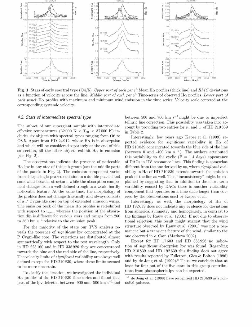
4.2. Stars of intermediate spectral type
The subset of our supergiant sample with intermediateeffective temperatures (32 000 K < Teff < 37 000 K) in-cludes six objects with spectral types ranging from O6 toO8.5. Apart from HD 24912, whose Hα is in absorptionand which will be considered separately at the end of thissubsection, all the other objects exhibit Hα in emission(see Fig. 2).
The observations indicate the presence of noticeableHα lpv in any star of this sub-group (see the middle partsof the panels in Fig. 2). The emission component variesfrom sharp, single-peaked emission to a double-peaked andsomewhat broader structure, while the absorption compo-nent changes from a well-defined trough to a weak, hardlynoticeable feature. At the same time, the morphology ofthe profiles does not change drastically and always consistsof a P Cygni-like core on top of extended emission wings.The emission peak of the mean Hα profiles is red-shiftedwith respect to vsys , whereas the position of the absorp-tion dip is different for various stars and ranges from 260to 360 km s−1 relative to the emission peak.
For the majority of the stars our TVS analysis re-veals the presence of significant lpv concentrated at theP Cygni-like core. The variations are distributed almostsymmetrically with respect to the rest wavelength. Onlyin HD 225 160 and in HD 338 926 they are concentratedtowards the blue and the red side of the line, respectively.The velocity limits of significant variability are always welldefined except for HD 210839, where these limits seemedto be more uncertain.
To clarify the situation, we investigated the individualHα profiles of the HD 210839 time-series and found thatpart of the lpv detected between -900 and -500 km s−1 and
between 500 and 700 km s−1might be due to imperfecttelluric line correction. This possibility was taken into ac-count by providing two entries for vb and vr of HD 210839in Table 2.
Interestingly, few years ago Kaper et al. (1999) re-ported evidence for significant variability in Hα ofHD 210839 concentrated towards the blue side of the line(between 0 and -400 km s−1 ). The authors attributedthis variability to the cyclic (P = 1.4 days) appearanceof DACs in UV resonance lines. This finding is somewhatdifferent from the one derived by us, where significant vari-ability in Hα of HD 210839 extends towards the emissionpeak of the line as well. This “inconsistency” might be ex-plained by suggesting that in addition to the short-termvariability caused by DACs there is another variabilitycomponent that operates on a time scale longer than cov-ered by the observations used by Kaper et al.
Interestingly as well, the morphology of Hα ofHD 192639 does not indicate any evidence for deviationsfrom spherical symmetry and homogeneity, in contrast tothe findings by Rauw et al. (2001). If not due to observa-tional selection, this result might suggest that the windstructure observed by Rauw et al. (2001) was not a per-manent but a transient feature of the wind, similar to theone observed in α Cam (Markova 2002).
Except for HD 17603 and HD 338926 no indica-tion of significant absorption lpv was found. RegardingHD 210839 and HD 192 639 this finding does not agreewith results reported by Fullerton, Gies & Bolton (1996)and by de Jong et al. (1999).8 Thus, we conclude that atleast for four out of the five stars in this group contribu-tions from photospheric lpv can be expected.
8 de Jong et al. (1999) have recognized HD 210 839 as a non-radial pulsator.

Markova et al.: Wind variability in O stars 7
Fig. 2. As Fig. 1, but for stars of intermediate spectral type (O6 to O8.5).
For all stars a genuine variability in the equivalentwidth of Hα has been found. Neglecting the possible con-tribution from absorption lpv (if present) we found thatthe (rather extreme) variations in the Hα net wind emis-sion can be accounted for by a 12% (HD 225 160) to 44%(HD 210839) variation in M .
HD 24 912 (ξ Per) was observed once in 1997, three timesin 1998 and once in 1999. The Hα profiles (lower-rightpanel of Fig. 2) appear completely in absorption, in con-trast to the profiles of the other sample stars of similarspectral type. The red wing is steeper than the blue oneand the absorption dip is blue-shifted with respect to thestellar rest frame. Profiles with similar signatures are typi-cal for stars with weaker winds where the Hα photosphericabsorption is partly filled in by wind emission.
The TVS of Hα consists of a blue-shifted, single-peaked component plus a double-peaked structure withmaximum amplitudes concentrated at the absorption core
and at the red extension of the profile. In an absorp-tion profile, a double-peaked TVS might indicate thepresence of radial velocity variability caused by pulsa-tions (Fullerton, Gies & Bolton 1996). Indeed, our mea-surements show that the velocity of the absorption coreof Hα varies around a mean value of -43±13km s−1 9.Since the position of the absorption dip does not seemto depend on the line strength (i.e., on the strength ofthe wind emission) we suggest that the observed radialvelocity variability is mostly (if not completely) due tochanges in the stellar photosphere and probably causedby pulsations (de Jong et al. 1999, 2001).
In addition to this, another variability componentseems to be present in HD 24 912, as indicated by theblue-shifted, single-peaked feature in the Hα TVS, locatedbetween -200 and -450 km s−1 . This velocity interval issimilar to the interval of the 2-d period variation estab-
9 The uncertainty in individual radial velocity measurementsequals to ±4.5 km s−1 , i.e., half the bin step of 0.2 A.

8 Markova et al.: Wind variability in O stars
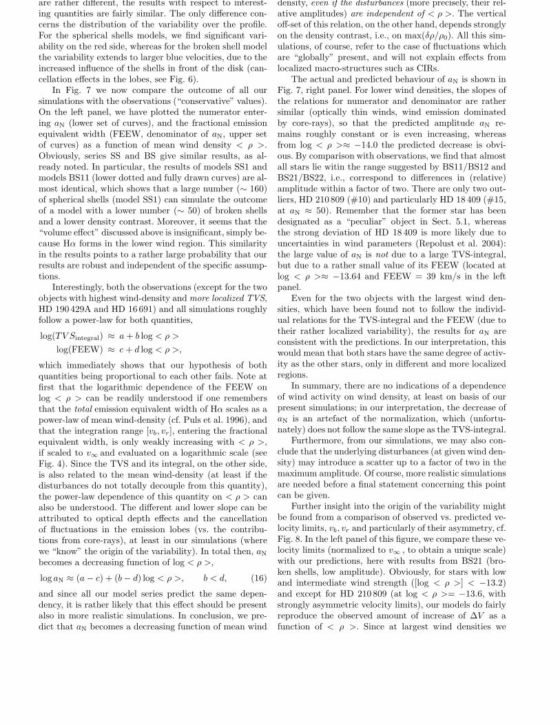
Fig. 3. As Fig. 1/2, but for stars of later spectral type (O9 to O9.7). Note the single-peaked, blue-shifted absorptionprofiles observed in HD 188209 in June, 1997 and February, 1998. Profiles with similar shape have not been observedby Israelian et al. (2000) throughout their long-term monitoring campaign. Note also the P Cygni-like profile observedin HD 18 409 in June, 1998. This profile is completely different from the rest of the time series and indicates a strongincrease in density in the innermost wind region.
lished by Kaper et al. (1997) and by de Jong et al. (2001),and both findings might have the same origin.
The EW of Hα varies between 1.3 and 1.8 A, ingood agreement with the limits derived by Kaper et al.(1997). Interpreted as due to variations in the mean winddensity, these limits comply with a ±16% variation inM , which is smaller than the error of the individualM estimates (±25%, Markova et al. 2004) and thus in-significant. Again, this finding is consistent with corre-sponding results from Kaper et al. (1997). Based on simul-taneous UV and optical observations of ξ Per, the latterauthors suggested that the EW variability of Hα is causedby the presence of large-scale, time-dependent structuresin the wind.
In summary, we conclude that the variability we haveobserved in ξ Per is a mixture of variations originatingboth from the photosphere (caused by non-radial pulsa-tions) and from the wind (presumably connected to theappearance of DACs).
4.3. Stars of late spectral type
The subset of sample stars of late spectral type (O9 toO9.7, Teff < 32 000 K) includes 6 objects. Five of themshow Hα profiles with similar morphology whereas an-other one - HD 210809 - exhibits a multitude of differentlyshaped Hα profiles and will be considered separately at theend of this subsection.

Markova et al.: Wind variability in O stars 9
The Hα profiles of HD 188209, BD+56 739,HD 209 975, HD 218 915 and HD 18 409 appear in ab-sorption, partly filled in by wind emission (see Fig. 3).The shape of the profiles can vary, from star to star andfor a given star as a function of time, from double-peakedabsorption with a central reversal peaked at the stellarrest frame to an asymmetric, blue-shifted absorption fea-ture, with the red wing being steeper than the blue one.Hα profiles with similar signatures have been found inearly B-type supergiants as well, e.g., Ebbets (1982).
No indication of extended emission wings has beenfound in this subgroup, except for BD +56739. This ob-ject shows weak, but clearly visible emission wings extend-ing to about ±1200 km s−1 , suggesting a relatively strongwind.10
All stars show evidence of real lpv in Hα. For partof the sample stars, the deviations are distributed almostsymmetrically with respect to the stellar rest frame, withmaximum amplitudes concentrated almost at the centralreversal, whereas for others (e.g. HD 209975), the varia-tions are stronger blueward from the rest wavelength. Inthe particular case of HD 209975 this blue-to-red asym-metry of the TVS might be explained by bluewards mi-grating DACs (Kaper et al. 1997). Two entries are givenfor HD 18409, since the blue velocity limit for significantHα variability is somewhat uncertain.
For none of the stars in this group we found evidenceof significant variability in the Heii λ6527 absorptionline. This finding is consistent with the results reportedby Fullerton, Gies & Bolton (1996) for the two starsin common, HD 188209 and HD 209 975. In contrast,Israelian et al. (2000) have reported evidence of quasi-periodic absorption lpv (with P = 6.4d) for HD 188209.Since the data-set used by Israelian et al. (2000) ismuch more extended than the one used by us and byFullerton, Gies & Bolton (1996), we consider their resultas more reliable. Thus we assume that in five out of thesix stars the observed variability in Hα is dominated bychanges in the wind and that only in HD 188209 a con-tribution from photospheric lpv is to be expected.
Our measurements show that the main source of lpvin Hα are changes in equivalent width. For all stars theM variations needed to account for the extreme changesdetected in Wem exceed the error of individual determina-tions and are therefore considered as real. As an example,for HD 188209 we derived upper and lower limits of 1.5and 1.75 x10⁻⁶M⊙ per year, respectively, in full agreementwith the estimates reported by Israelian et al. (2000).
HD 210 809. The individual spectra, shown in the mid-dle part of the corresponding plot in Fig. 3, indicate thepresence of dramatic lpv in Hα. The profiles change froma relatively weak absorption trough with a flat core viaan ordinary/reverse P Cygni-like feature to a triple emis-sion structure. In addition, strong emission wings extend-
10 Weak emission wings (±900 km s−1 ) might be present alsoin HD 209 975.
ing to ∼1500 km s−1 are clearly visible. Line profile vari-ability with similar signatures has been discussed as anindication of long-lived, large-scale wind density pertur-bation(s), which co-rotate with the star, giving rise to ad-ditional line emission at various frequencies (Rauw et al.2001, and references therein).
As might be expected from the observations, the dis-tribution of lpv in Hα is asymmetric with respect to therest wavelength, with maximum amplitudes concentratedat the P Cygni-like core. The smaller amplitude devia-tions located between 600 and 900 km s−1 are caused bythe appearance of a bump on the red emission wing in theJune 1998 line profile.
From the TVS of Heii λ6527 , we found no indication ofsignificant photospheric lpv, suggesting that the observedvariations in Hα are caused by changes in the wind.
Although the observations give clear evidence for de-viations from spherical symmetry, we applied our line-synthesis code (based on a spherical model) to find con-straints on the mass-loss rate variability of the star.Fitting particularly the first and the last profile of thetime series by model calculations, we found that the ex-treme variations in Wem can be reproduced by variationsof ±20% in M .
5. Hα line-profile variability as a function of
stellar and wind parameters
In order to obtain further clues concerning the origin ofwind variability (as traced by Hα) in O supergiants, weexamined various correlations between line profile param-eters and parameters of the TVS of Hα, on the one hand,and fundamental stellar and wind parameters of the sam-ple stars, on the other. To search for such correlations, weused the Spearman rank-order correlation test, described,for example, by Press et al. (1992). The main advantageof this test is that in addition to the correlation coeffi-cient (more precisely, the linear correlation coefficient ofranks) it also calculates the statistical significance of thiscorrelation (expressed as the two-sided significance of itsdeviation from zero), without any assumption concerningthe distribution of uncertainties in the individual quanti-ties.
5.1. Hα profile shape as a function of spectral type
An inspection of the mean Hα profiles of the sample stars(all supergiants!), displayed in Figures 1 to 3, shows thatthese profiles evolve as a function of spectral type froma slightly asymmetric emission with a peak value red-shifted with respect to vsys , via an emission feature witha P Cygni-like core, to a feature in absorption (with orwithout central emission reversal). In stars of early andintermediate spectral type extended emission wings canbe seen, while in stars of late spectral type the presenceof such wings is rare.
There are two stars that deviate from this behaviour,HD 24 912 and HD 210809. The former one exhibits a

10 Markova et al.: Wind variability in O stars
pure absorption profile instead of a P Cygni-like profile(see Fig. 2). Consequently, its Hα line resembles muchmore those profiles from luminosity class III than fromluminosity class I objects of the same spectral type. Aswe have already pointed out in Paper I, the parametersof HD 24 912 are somewhat insecure due to the uncertaindistance - HD 24 912 is not a member of PerOB2 but arunaway star (Gies 1987). Thus it is rather likely that thediscrepancy in profile shape is due to an erroneous (re-)assignment in luminosity class (Herrero et al. 1992) andsuggest that the original value as assigned by Walborn(1973), luminosity class III, is more appropriate (see alsoRepolust et al. 2004).
The second outlier, HD 210809, shows a P Cygni-like profile instead of an absorption profile partly filledin by wind emission. This is the only star in the sam-ple for which our observations suggest a strong devia-tion from spherical symmetry. From the similarity to theHα and Heii 4686 time-series of HD 192639 observedand discussed by Rauw et al. (2001) (single and doublepeak structure in emission), we speculate that also herea “confined co-rotating wind” is present. This interpreta-tion, if correct, would explain the “peculiar” shape of themean Hα profile derived by us. Hereafter, we will refer toHD 24 912 and HD 210 809 as to “peculiar” stars.
The observed evolution of Hα in O-supergiants withspectral type (actually with Teff ) is in fair agreementwith results from theoretical line-profile computations per-formed in terms of NLTE, spherically symmetric, smoothstellar wind models, although the strength of the observedP Cygni-like core cannot be reproduced in most cases (e.g.,Repolust et al. 2004).11 The main drivers of this evolu-tion are: decreasing line emission caused by decreasingwind density (since M decreases with decreasing Teff andlogL/L⊙ , see Vink et al. 2000) and decreasing contribu-tion of the Heii λ6560blend. (In contrast, purely pho-tospheric Hα profiles of a given luminosity class do notchange significantly as a function of Teff , because in thistemperature regime the photospheric ionization fractionof neutral hydrogen remains fairly constant.) Outliers canoccur either as a result of strong deviations from spheri-cal symmetry and homogeneity in the wind (due to, e.g.,fast rotation, CIRs, clumps) or as a result of an erro-neous spectral type/luminosity class classification or un-certain/wrong parameters.
5.2. Red-shifted emission-peaks
Our observations suggest that the position of the emissionpeak of the Hα profiles of O supergiants depends on thestrength of the wind: for stars with weaker winds (Hα inabsorption with/without central reversal) this peak is cen-
11 This problem has not been solved satisfactorily so far. Inparticular, it is still unclear if the blue-shifted absorption coreis solely related to the Heii blend or other effects (clumps,deviations from 1-D geometry) have to be accounted for addi-tionally.
tered almost at the rest wavelength, whereas for stars withstronger winds (Hα in emission) it is red-shifted instead.This observation is supported by results of the correlationanalysis, which shows that the velovity of the emissionpeak,ve correlates significantly with < ρ >, (.79/0.0007)and in addition with Teff (.82/0.0003).12
Hereafter, numbers in brackets denote the Spearmanrank correlation coefficient and the two-sided significanceof its deviations from zero. Since the latter quantity mea-sures the probability to derive a given correlation coeffi-cient from uncorrelated data, smaller values mean highersignificance of the correlation.
Red-shifted emission peaks have been observed in UVresonance lines of O-type stars, where this finding (in par-allel with the presence of an extended absorption trough)can been explained in terms of “micro-turbulence” effects,with vmicro of the order of 0.1 v∞ (e.g., Hamann 1980 andreferences therein, Groenewegen & Lamers 1989). On afirst glance, the phenomenon seen in Hα seems to be some-what similar. In contrast to the situation for UV resonancelines, however, our Hα profile simulations meet no prob-lem in reproducing the red-shifted peak, even if the shiftis large, without any inclusion of micro-turbulence. Thiscan be seen clearly by comparing theoretical profiles withobservations, e.g., Markova et al. (2004); Repolust et al.(2004). A closer inspection of the profile formation pro-cess reveals that the apparent shift of the emission peakresults (at least in our simulations) from the interactionbetween the red-side of the Stark-broadened photosphericprofile and the wind emission. Let us note that we do notexclude the presence of micro-turbulence but that we sim-ply do not need it to reproduce the observed amount ofve.
5.3. Properties of the TVS as a function of stellar and
wind parameters
Before investigating the properties of the Hα TVS for oursample stars, let us point out that all results outlined be-low refer to the “conservative case” (see Sect. 3). Althoughthe “non-conservative” data have not been analyzed in de-tail, they are included in the corresponding plots and wewill comment on their influence on the final outcome.
5.3.1. Distribution of Hα line-profile variability in
velocity space
In Figure 4 we show the blue and red velocity limits (leftpanel, dashed) and the velocity width ∆V (absolute value,right panel) of Hα lpv as a function of the mean winddensity. Thick vertical lines correspond to the projectedrotational speed, ±v sin i. Asterisks refer to the conser-vative estimates for ∆V , while diamonds mark the non-
12 In this particular case and because of the reasons outlinedabove, the “peculiar” stars HD 210 809 and HD 24 912 havebeen discarded from the correlation analysis.

Markova et al.: Wind variability in O stars 11
Fig. 4. Blue and red velocity limits (left panel) and velocity width (right panel) of significant lpv in Hα, as a functionof mean wind density of the sample stars. Thick vertical lines denote the corresponding projected rotational velocity,±v sin i. Asterisks refer to the conservative estimates for ∆V , while diamonds mark the non-conservative ones.
Table 2. Hα line profile and variability parameters. N denotes the number of available spectra. ve is the velocityof the emission peak while vb, vr are the “blue” and “red” velocity limits of significant variability. All velocity dataare measured with respect to the stellar rest frame and given in km s−1 . σ0 is the standardized dispersion of thecorresponding time-series. rmax (expressed in R⋆ ) denotes the upper limit in physical space where significant variationsin Hα are present. Wem is the mean equivalent width of net wind emission and its standard deviation, both givenin A. Wphot is the equivalent width of the photospheric component. M min and M max (in 10−6 M⊙ /yr) denote the
corresponding limits if the observed variability is attributed to variations in M alone, while ∆M is the amplitude ofthis variability expressed in percents of M min. < ρ > is the mean wind density (Eq. 12), and AN and aN are the meanand the fractional amplitudes (Eqs. 10 and 9), respectively.
Object # N lpv(a) ve σ0*100. [ vb, vr] rmax Wem/Wphot M min M max ∆M log < ρ > AN aN
HD 190 429 1 9 no 210 0.93 [ -491, 234] 1.23 10.99±0.63/3.23 13.0 14.0 8% 13.16 2.24 6.07± 0.03[-491, 363] 2.09 5.73±0.03
HD 16 691 2 3 no 223 0.51 [ -448, 266] 1.22 10.87±0.81/3.23 12.0 13.0 8% 13.13 2.89 7.17± 0.02HD 14 947 3 4 no 82 0.50 [ -704, 747] 1.43 9.35±0.90/3.24 14.5 16.0 10% 13.27 1.90 7.84± 0.02HD 210 839 4 11 yes 220 0.67 [ -633, 478] 1.40 4.74±0.55/3.00 6.8 9.8 44% 13.42 1.92 11.63± 0.03
[-838, 665] 1.61 1.73 12.95±0.04HD 192 639 5 7 no 140 0.67 [ -393, 460] 1.27 6.15±0.52/3.02 4.7 5.4 16% 13.38 3.36 13.77± 0.03HD 17 603 6 7 yes 210 0.60 [ -373, 619] 1.27 4.04±0.49/2.84 5.5 7.2 31% 13.56 1.87 12.49± 0.05HD 24 912 7 5 yes -50 0.40 [ -419, 309] 1.12 1.36±0.14/2.85 4.5 5.2 16% 13.77 1.09 15.32± 0.14HD 225 160 8 4 no 140 0.46 [ -491, 384] 1.33 4.51±1.04/2.62 5.1 5.7 12% 13.45 3.21 15.61± 0.02HD 338 926 9 3 yes 140 0.44 [ -352, 362] 1.21 4.54±0.38/2.61 4.5 5.4 20% 13.59 2.48 11.78± 0.03HD 210 809 10 5 no 10 0.63 [ -336, 909] 1.15 3.63±0.63/2.59 3.2 4.5 41% 13.60 2.77 24.11± 0.05HD 188 209 11 6 yes -6 0.72 [ -176, 144] 1.09 1.56±0.19/2.18 1.5 1.8 17% 13.87 2.67 16.37± 0.08BD+56 739 12 3 no 13 0.69 [ -295, 96] 1.12 1.78±0.31/2.18 2.1 2.5 19% 13.80 2.84 24.66± 0.72HD 209 975 13 4 no 26 0.48 [ -277, 220] 1.09 1.36±0.29/2.18 1.5 1.9 27% 13.92 1.90 20.85± 0.10HD 218 915 14 6 no -8 0.70 [ -149, 206] 1.07 1.81±0.24/2.18 1.6 2.0 25% 13.91 2.51 17.14± 0.10HD 18 409 15 5 no 3 0.70 [ -274, 268] 1.08 1.40±0.47/2.17 1.5 2.2 47% 13.64 3.39 47.18± 0.11
conservative cases. In combination with the results de-scribed in Sect. 4, these figures indicate that:
i) for all stars the Hα lpv extends beyond the limits de-termined by stellar rotation and thus must be linkedto the wind;
ii) in most of our sample stars the variations occur eithersymmetrically (within the error) with respect to therest wavelength or with a weak blue-to-red asymmetry.For two objects, HD 17 603 and HD 210809, the TVShas a noticeable red-to-blue asymmetry, while in other
two stars, HD 190429A and HD 16 691, the variationsare stronger and more extended bluewards of the restwavelength.
iii) the velocity width for significant variability in Hα islarger in stronger winds than in weaker ones. Thereare two stars that deviate from this rule: HD 190429Aand HD 16 691 which exhibit variations over a veloc-ity interval that is considerably smaller than expectedfrom the strength of their winds.

12 Markova et al.: Wind variability in O stars
Fig. 5. Examples of significant correlations between the fractional amplitude of deviations, aN, as defined in the presentstudy, and stellar and wind parameters of the sample stars. Distributions of the mean amplitude AN are shown forcomparison. Asterisks refer to the conservative estimates, while diamonds mark the non-conservative ones. Positionsof the two “peculiar” stars are denoted by ‘P’.
Further analysis of the velocity data listed in Table 2shows that in all sample stars significant lpv in Hα occursbelow 0.3 v∞ . Converted to physical space, this yields anupper limit of roughly 1.5 R⋆ for the observed variability.Additionally, we found a significant correlation betweenrmax and log < ρ >, (0.87/0.00001). This result as wellas the possible dependence between ∆V and log < ρ >(0.62±0.01) are readily understood in terms of an increas-ing wind volume which contributes to the Hα emission, asa function of wind density.
We are aware of the fact that due to observationalselection effects and other uncertainties affecting the de-termination of the velocity limits, the results describedabove might be questioned. However, note that: (i) theprobability to obtain a symmetric TVS for a star with astrongly asymmetric wind, using snapshot observations,is very low; (ii) the established correlations between ∆Vand log < ρ > (right panel of Figure 4) and betweenrmax and log < ρ > are both physically reasonable, whichin turn supports the reliability of the limits determinedby us; (iii) although the limits and hence ∆V changeswhen non-conservative instead of conservative estimates
are considered, the final outcome does not change (seeFigure 4 and Table 2).
Thus, we assume that the velocity limits determinedhere do not seem to be strongly biased by either observa-tional selection or uncertainties in the measured quanti-ties. (But see also the next sub-section.)
If a good temporal resolution of the variability time-scale is provided, the velocity distribution of lpv in Hα willallow to obtain significant information about the wind ge-ometry (Harries 2000). On the other hand, and as we shallshow later on (see Sect 6), even in the case of snapshotobservations some hints about wind structures can be de-rived.
5.3.2. Mean and fractional amplitudes of deviations as
a function of stellar and wind parameters
Our TVS analysis shows that the mean amplitude of devi-ations always exceeds the corresponding threshold for sig-nificant variability, indicating genuine variability in Hα.The actual values of AN range between 1 and 4 percent ofthe continuum flux, without any clear evidence for depen-dence on stellar and wind parameters of the sample stars.

Markova et al.: Wind variability in O stars 13
This result is illustrated in the upper left panel of Fig. 5,where the estimates for AN are shown vs. log < ρ >.
This independence of AN on log < ρ > can have atwofold interpretation: First, if the mean amplitude is areasonable measure for wind variability, then the windvariability is actually more or less independent on wind-strength. Second, the mean amplitude is not the appro-priate tool to compare the strengths of Hα lpv.
Leaving aside these two possibilities, let us first con-sider the following problem. If we assume that the sourcesof observable variability are distributed over a certain vol-ume which increases as a function of mean wind den-sity (as it is suggested from the increase of rmax withlog < ρ >), then one should expect that also AN shouldincrease with mean density, since the numerator of thisquantity (the integral over (TV S − σ2
0)0.5) increases as a
function of the emitting volume, whereas the denominatorcorresponds to an (increasing) 1-D quantity only. The factthat the observed mean amplitude is actually independenton log < ρ > shows that such a simple model is not suf-ficient to explain the observations. We will come back tothis point again in Sect. 6.
In contrast to the established independence of themean amplitude on wind density, our analysis showsthe presence of a negative correlation between the frac-tional amplitude of deviations, aN, and a number of stel-lar/wind parameters. Scatter plots for the strongest cor-relations, with Teff (0.92/0.000001) and with log < ρ >(0.80/0.0003), are illustrated in Fig. 5. In particular, thedecrease of aN with increasing log < ρ > suggests thatthe observed variability per unit fractional net emission issmaller in denser winds than in thinner ones.
The reliability of the derived values of the mean andfractional amplitudes has been checked in two ways: first,we examined the stability of the results against effectscaused by observational selection and other uncertaintiesin the measured quantities; second, we checked the va-lidity of the assumptions underlying our definitions of AN
and aN.In particular, to clarify to what extent these quanti-
ties (and again ∆V ) might be influenced by observationalselection effects, we proceeded as follows:
i) For the two stars with longest time series we reducedthe number of spectra by about 30% while keeping thetwo most “extreme” profiles. The effect of this datamanipulation on the TVS parameters was found to beinsignificant.
ii) For the stars with longer time series (N > 6) we re-moved: (a) the spectrum with minimum Hα emission;(b) the spectrum with maximum Hα emission and (c)the two spectra with minimum and maximum windemission and re-calculated the TVS. In all the threecases the new estimates of σ0 and ∆V turned out tobe quite similar to the original ones: the establisheddifferences were less than a few percent. At the sametime the TVS amplitudes changed by less than 10 per-cent for stars with Hα in emission and by about 15
to 20 percent for stars with Hα in (partly re-filled)absorption. The effect of these changes was again in-significant concerning the final results for ∆V , AN andaN.
Let us finally point out that the estimates of the TVSparameters are expected to depend strongly on the qual-ity of the data used (i.e., on σ0). To simulate higherS/N (about two times higher than the original values) wesmoothed the spectra in each time series, using a boxcaraverage with a width of 4 pixels, and analyzed them inthe same way as the original spectral series. Interestingly,while the effect of this data manipulation on the estimatesof ∆V was surprisingly small (less than ±12 percent ofthe original values), the reaction of the TVS amplitudesturned out to be quite strong: both AN and aN, averagedover the whole sample, decreased by 37 and 33 percent,respectively, compared to their original values.13 Most im-portantly, however, the new estimates of ∆V , AN and aNwere found to obey similar dependences on log < ρ > asimplied by the original data set.14
Summarizing we conclude that the derived indepen-dence of AN on stellar and wind parameters as well asthe negative correlations between these parameters andaN cannot be explained in terms of either observationalselection or uncertainties in the measured quantities.
6. Simulations of lpv in Hα
In order to account for the systematic difference in thestrength of Hα as a function of spectral type/mean winddensity, in Sect. 3 we optimized the fractional amplitudeof deviations by normalizing the integral over the TVS toa quantity which we called fractional emission equivalentwidth, FEEW (see Eq. 9).
The parameter aN defined in this way is thus a mea-sure for the observed variability (represented by the cor-responding TVS) per unit fractional wind emission andhas been used in the previous section to investigate thedependence of the observed variability on wind density.The results obtained might be interpreted as an indica-tion that denser winds are less active than thinner winds,a finding which would give firm constraints on present hy-drodynamical simulations.
Note, however, that (i) our definition of aN implicitlyassumes that the TVS amplitude is proportional to thecorresponding amount of wind-emission and that (ii) thisassumption has not been checked so far. In particular, ifthis assumption was justified, the derived values of aNwould provide a robust measure for the “observed” degreeof wind-variability, as it is true for the photospheric lpv’sdescribed in terms of aF.
13 Part of this decrease might be due to the fact that thecontribution of higher frequency variability (if any) has beenreduced by smoothing.14 This result might no longer be true if large differences inthe quality, i.e., in the standardized dispersion of the spectraltime-series, σ0, were present (the requirement of homogeneity).

14 Markova et al.: Wind variability in O stars
Table 3. Summary of simple 1-D simulations. Models de-noted by“SS” refer to spherical shells, models denoted by“BS” to broken shells, respectively.
Series properties max(δρ/ρ0)
SS1 δv = 0.5vth(H) ±0.7SS2 δv = 1.0vth(H) ±0.7BS11 δm = const, ∆p(core) = 0.1 R⋆ ±0.35BS12 δm = const, ∆p(core) = 0.1 R⋆ ±0.7BS21 δm = const, ∆p(core) = R⋆ ±0.35BS22 δm = const, ∆p(core) = R⋆ ±0.7SS3 δm = const ±0.35
6.1. 1-D model simulations
Thus, a test of our hypothesis is urgently required. Ideally,such a test would make use of at least 2-D models of insta-ble winds, since the assumption of 1-D shells most proba-bly overestimates the actual degree of variability.
Since 2-D simulations involving a consistent physicaldescription are just at their beginning (Dessart & Owocki2003) and since, to our knowledge, even for somewhatsimpler multi-dimensional models no investigation con-cerning the dependence on wind parameters is available(Sect. 6.2), we have proceeded in the following way.
We have constructed a large number of very simplewind-models with variable Hα wind emission, in completeanalogy to our stationary description (Paper I). The re-sulting profiles (10 per model) have been analyzed in thesame way as the observed ones, i.e., by means of the TVS-analysis as described in Sect. 3. To allow for a directcomparison with results from our observations, we haveadded artificial Gaussian noise to the synthesized profiles(S/N = 200, which is a typical value), and have re-sampledthe synthetic output onto constant wavelength bins corre-sponding to an average resolution of 15 000.
In order to account for the effects of wind disturbancesof different size and density contrast in different geome-tries, we calculated various series of models: three consist-ing of spherical shells (series SS) and four consisting ofbroken shells (i.e., clumps, series BS1 and BS2). A sum-mary of the various models and their designation is givenin Table 3.
All simulations are based on our (quiet) model forHD 188209 with M = 1.6·10−6M⊙/yr (cf. Paper I). In or-der to investigate the reaction of the TVS of the syntheticprofiles as a function of wind-strength we calculated, foreach model series, 9 different models, with ∆ log M ≈0.1, particularly at 0.8, 1.25, 1.6, 2.0, 2.5, 3.2, 4.0, 5.0 and10.0 ·10−6M⊙/yr. In this way, profile shapes varying frompure absorption via P Cygni type to pure emission havebeen obtained, covering all “observed” mean wind densi-ties.
In all these models, only the density was allowed tobe variable, whereas the velocity field and thus the NLTEdeparture coefficients (as a function of velocity) have beenkept at their original value.
In a first step (series SS1/SS2), we used the most sim-plistic approach of disturbing the density, namely we var-ied this quantity in a random way as a function of ra-dius only, i.e., we assumed spherical shells. This step, al-though rather unrealistic, has been performed particularlyto check the stability of results from somewhat more “so-phisticated” models (series BS1/BS2), which are describedbelow.
The variations are defined in such a way as to allowfor both positive and negative disturbances around the“quiet” model, in order to preserve the mean profile. Wedivided the wind into shells of equidistant velocity range,δvshell, where
δvshell = c · vth(H), c = 0.5, 1 (13)
with vth(H) the thermal velocity of hydrogen. The differ-ent multipliers c define two different series, SS1 and SS2,respectively. Inside each of the shells, the density has beenperturbed by a maximum amplitude of ±70%,
ρ = ρ0(1 + δρ/ρ0), δρ/ρ0 = −0.7 + 1.4 · RAN, (14)
with ρ0 the stationary density and ran a random numberuniformly drawn from the interval [0,1]. The specific max-imum amplitudes (for series SS, but also for series BS, seebelow) have been chosen in such a way that the resultingTVS-integrals and FEEWs are (roughly) consistent withthe observed values. Lower maximum amplitudes wouldresult in a too low degree of variability, and higher onesin too large values.
Note that the density contrast has been assumed tobe constant within each of the shells, i.e., the number ofdrawn variables is given by the total number of shells,which is of the order of 80 for v∞ = 1650 km/s and c =1. Note also that only the wind has been allowed to bevariable, i.e., we considered perturbations only outside thesonic point, located roughly at 20 km s−1 .
In this way then, different and random amplitudeswithin the maximum range δρ/ρ0 ∈ [−0.7, 0.7] are createdfor each individual shell. To allow for a temporal variabil-ity of the resulting profiles at “random” observation times(remember that our observations are typically separatedby much more that one wind flow time) we performed,for each model, 10 simulations with different initializationof ran and different locations of the contributing shells.The resulting 10 different profiles have been analyzed sub-sequently by means of the TVS method (an example isgiven in Fig. 6).
Model series SS suffers from (at least) two major prob-lems. At first, the assumption of spherical shells mightamplify the lpv at all frequencies, since, especially in thewind lobes, there is only a weak chance that fluctuationswill cancel out due to statistical effects. Second, our simu-lations define equal amplitudes of disturbance inside shellsof equidistant range in velocity space. Accounting for therather steep increase in velocity inside and the flat veloc-ity field outside, this means that the contributing volumeper shell is strongly increasing with radius, which mightgive too much weight to disturbances in the outer wind.

Markova et al.: Wind variability in O stars 15
Fig. 7. Left panel: “Observed” values of the numerator entering aN (TVSintegral, asterisks) and of the fractionalemission equivalent width (denominator of aN, crosses), compared with simulated quantities, as a function of meanwind density log < ρ >. The dotted curves correspond to the simulations with spherical shells and constant δv spacing(SS1/SS2), and the other curves to the somewhat more realistic simulations accounting for broken shells and constantδm, BS11/BS12 (fully drawn) and BS21/BS22 (dashed). Note that inside each series of simulations the maximumamplitude of density-fluctuations, δρ/ρ0, is identical, i.e., independent on wind density. Right panel: As left, but forthe fractional amplitude aN (in %). The object numbers correspond to the entries given in Table 2.In both panels, the special symbols correspond to the data resulting from our TVS-analysis of the 3-D models presentedby Harries (2000), cf. Sect. 6.2 (diamonds: spiral structure; triangles: clumpy structure).
Fig. 6. As Fig. 1, but for synthetic profiles correspond-ing to model BS11 (broken shells, low amplitude) ofHD 188 209, at M = 2.5 · 10−6M⊙/yr (see text).
To “cure” both problems, we have calculated four ad-ditional model series, which should be more realistic thanthe above ones. At first, the spherical symmetry is bro-
ken by the following modification.15 For the core-rays, weassume coherent shells (blobs), either of a relatively smalllateral extent, ∆p ≈ R⋆/10 (series BS1) or of a larger ex-tent, ∆p = R⋆ (series BS2). For each of the non-core rays(distributed roughly logarithmically), on the other hand,we assume different locations of the density variations perray, to simulate the presence of broken shells. The lattermodification results in a lower TVS particularly in the redpart of the profiles, due to cancellation effects. Note thatwe have convinced ourselves that different distributions ofnon-core rays gave very similar results.
In order to avoid the volume effect, instead of assumingδρ/ρ0 as random, however constant per shell of thicknessδv = const, we now require that the random perturbationsshould occur in shells of equal mass,
δmshell = 4πr2ρdr, (15)
with roughly 50 (broken) shells per model. Inside eachbroken δm shell, the density fluctuations are evaluatedas above. For each of our simulations BS1 and BS2, wehave used two different values for the maximum ampli-tude, max(δρ/ρ0) = ±0.35 and ±0.7 (BS11/BS21 andBS12/BS22, respectively), which gives a fair consistencywith the range of observed variability.
Before we discuss the results in detail, let us alreadypoint out here the major outcome. Although the assump-tions inherent to the various model series (SS vs. BS)15 Remember that the radiative transfer is performed in theusual p−z geometry, with impact parameter p and height overequator z. The so-called core rays are defined by p ≤ R⋆, andthe non-core rays passing both hemispheres of the wind lobesby p > R⋆.
16 Markova et al.: Wind variability in O stars
are rather different, the results with respect to interest-ing quantities are fairly similar. The only difference con-cerns the distribution of the variability over the profile.For the spherical shells models, we find significant vari-ability on the red side, whereas for the broken shell modelthe variability extends to larger blue velocities, due to theincreased influence of the shells in front of the disk (can-cellation effects in the lobes, see Fig. 6).
In Fig. 7 we now compare the outcome of all oursimulations with the observations (“conservative” values).On the left panel, we have plotted the numerator enter-ing aN (lower set of curves), and the fractional emissionequivalent width (FEEW, denominator of aN, upper setof curves) as a function of mean wind density < ρ >.Obviously, series SS and BS give similar results, as al-ready noted. In particular, the results of models SS1 andmodels BS11 (lower dotted and fully drawn curves) are al-most identical, which shows that a large number (∼ 160)of spherical shells (model SS1) can simulate the outcomeof a model with a lower number (∼ 50) of broken shellsand a lower density contrast. Moreover, it seems that the“volume effect” discussed above is insignificant, simply be-cause Hα forms in the lower wind region. This similarityin the results points to a rather large probability that ourresults are robust and independent of the specific assump-tions.
Interestingly, both the observations (except for the twoobjects with highest wind-density andmore localized TVS,HD 190429A and HD 16 691) and all simulations roughlyfollow a power-law for both quantities,
log(TV Sintegral) ≈ a+ b log < ρ >
log(FEEW) ≈ c+ d log < ρ >,
which immediately shows that our hypothesis of bothquantities being proportional to each other fails. Note atfirst that the logarithmic dependence of the FEEW onlog < ρ > can be readily understood if one remembersthat the total emission equivalent width of Hα scales as apower-law of mean wind-density (cf. Puls et al. 1996), andthat the integration range [vb, vr], entering the fractionalequivalent width, is only weakly increasing with < ρ >,if scaled to v∞ and evaluated on a logarithmic scale (seeFig. 4). Since the TVS and its integral, on the other side,is also related to the mean wind-density (at least if thedisturbances do not totally decouple from this quantity),the power-law dependence of this quantity on < ρ > canalso be understood. The different and lower slope can beattributed to optical depth effects and the cancellationof fluctuations in the emission lobes (vs. the contribu-tions from core-rays), at least in our simulations (wherewe “know” the origin of the variability). In total then, aNbecomes a decreasing function of log < ρ >,
log aN ≈ (a− c) + (b− d) log < ρ >, b < d, (16)
and since all our model series predict the same depen-dency, it is rather likely that this effect should be presentalso in more realistic simulations. In conclusion, we pre-dict that aN becomes a decreasing function of mean wind
density, even if the disturbances (more precisely, their rel-ative amplitudes) are independent of < ρ >. The verticaloff-set of this relation, on the other hand, depends stronglyon the density contrast, i.e., on max(δρ/ρ0). All this sim-ulations, of course, refer to the case of fluctuations whichare “globally” present, and will not explain effects fromlocalized macro-structures such as CIRs.
The actual and predicted behaviour of aN is shown inFig. 7, right panel. For lower wind densities, the slopes ofthe relations for numerator and denominator are rathersimilar (optically thin winds, wind emission dominatedby core-rays), so that the predicted amplitude aN re-mains roughly constant or is even increasing, whereasfrom log < ρ >≈ −14.0 the predicted decrease is obvi-ous. By comparison with observations, we find that almostall stars lie witin the range suggested by BS11/BS12 andBS21/BS22, i.e., correspond to differences in (relative)amplitude within a factor of two. There are only two out-liers, HD 210809 (#10) and particularly HD 18 409 (#15,at aN ≈ 50). Remember that the former star has beendesignated as a “peculiar” object in Sect. 5.1, whereasthe strong deviation of HD 18 409 is more likely due touncertainties in wind parameters (Repolust et al. 2004):the large value of aN is not due to a large TVS-integral,but due to a rather small value of its FEEW (located atlog < ρ >≈ −13.64 and FEEW = 39 km/s in the leftpanel.
Even for the two objects with the largest wind den-sities, which have been found not to follow the individ-ual relations for the TVS-integral and the FEEW (due totheir rather localized variability), the results for aN areconsistent with the predictions. In our interpretation, thiswould mean that both stars have the same degree of activ-ity as the other stars, only in different and more localizedregions.
In summary, there are no indications of a dependenceof wind activity on wind density, at least on basis of ourpresent simulations; in our interpretation, the decrease ofaN is an artefact of the normalization, which (unfortu-nately) does not follow the same slope as the TVS-integral.
Furthermore, from our simulations, we may also con-clude that the underlying disturbances (at given wind den-sity) may introduce a scatter up to a factor of two in themaximum amplitude. Of course, more realistic simulationsare needed before a final statement concerning this pointcan be given.
Further insight into the origin of the variability mightbe found from a comparison of observed vs. predicted ve-locity limits, vb, vr and particularly of their asymmetry, cf.Fig. 8. In the left panel of this figure, we compare these ve-locity limits (normalized to v∞ , to obtain a unique scale)with our predictions, here with results from BS21 (bro-ken shells, low amplitude). Obviously, for stars with lowand intermediate wind strength ([log < ρ >] < −13.2)and except for HD 210 809 (at log < ρ >= −13.6, withstrongly asymmetric velocity limits), our models do fairlyreproduce the observed amount of increase of ∆V as afunction of < ρ >. Since at largest wind densities we

Markova et al.: Wind variability in O stars 17
Fig. 8. Left panel: Observed blue and red velocity limits, vb, vr (conservative and non-conservative values) in units ofv∞ , as a function of mean wind-density, compared with results from simulation BS21 (dashed).Right panel: Observed asymmetry, (vr − |vb|)/(vr + |vb|) (conservative values, black dots), compared with simulations(asterisks: BS21, squares: BS11, crosses: SS3). The object numbers correspond to the entries given in Table 2. Thediamond and triangle refer to the data resulting from our TVS-analysis of the 3-D spiral and clumpy model presentedby Harries (2000), cf. Sect. 6.2.
have only two objects in our sample, it is not clear atpresent whether their discrepant behaviour is peculiar ornot. Thus, except for the outliers, it might be concludedthat the observed variability results from effects which arepresent everywhere in the wind, in accordance with ourmodels. This conclusion seems to be also supported bythe fact that HD 210 809 deviates from our predictions:for this star our observations have suggested the presenceof large-scale wind disturbances which are localized ratherthan uniformly distributed over the wind volume.
The right panel of Fig. 8, however, shows also theshortcomings of our models. Plotted is the asymmetry ofvb, vr by means of the expression (vr−|vb|)/(vr+|vb|) (neg-ative values correspond to blue-to-red, positive values tored-to-blue asymmetries, respectively). Let us firstly dis-cuss the “theoretical” predictions. We have plotted the re-sults for model series BS21 (asterisks), BS11 (squares) andfor a model which has been constructed additionally forthis comparison, namely a model with spherical shells andδm = const(SS3, crosses). All three models have the samemaximum amplitude, max(δρ/ρ0) = ±0.35. Not surpris-ingly, the last model shows the least asymmetry, whereasmodel BS21 shows the largest one, due to the large lateralextent of the assumed broken shells in front of the stellardisk. Note that most models show a blue-to-red asymme-try, even those with spherical shells, whereas in no case aredwards asymmetry is found. This predicition, of course,results from cancellation effects in the lobes, comparedto the situation for core-rays. For large wind-densities,all models converge to small or even negligible asymme-try, because of the increasing influence of the lobes. Formodel SS3 (spherical shells), symmetry is reached earliest,roughly at log < ρ >= −13.5.
With respect to the observations, the situation is asfollows. At low and intermediate wind densities, only four
objects display a significant asymmetry, mostly to the red,where the highest degree is found for HD 210809 (#10,see above). The majority of stars, however, show eithera small degree of asymmetry (both to the blue and tothe red) or behave symmetrically. The predictions of se-ries SS3 are closest to this behaviour. Let us point outalready here that a symmetric TVS at low wind densitiescan be alternatively explained by models with co-rotatingstructures (e.g., CIRs), as will be discussed later on. Forthe two stars with larger wind densities, the predictionsdefinitely deviate from what has been observed.
In Sect. 5.3.2 it turned out that the mean amplitude ofdeviations, AN, seems to be uncorrelated with mean winddensity, at least for our sample. We speculated that if thesources of wind variability were (uniformly) distributedover the contributing wind volume, one should see a pos-itive correlation. By means of our simple models, we cancheck this conjecture now and may find additional con-straints on the origin of wind variability.
Fig. 9 shows the behaviour of the simulated meanamplitude as a function of mean wind density, for se-ries BS11/BS12, series BS21/BS22 and SS3, respectively.Actually, AN is strongly correlated with < ρ >, where thevertical offset is a function of (relative) amplitude δρ/ρ0.On a first glance, we might conclude that the observedvalues are again (i.e., as we have found for aN) consistentwith the models, if we allow for a variation in amplitudeof roughly a factor of two.
A closer inspection, on the other hand, reveals thatat least for two low density objects (HD 188209, #11and HD 218915, #14) there is the following problem. Themean amplitudes of these objects are consistent with oursimulations with larger δρ/ρ0 (BS22). Concerning the frac-tional amplitudes, aN, however, they are consistent with

18 Markova et al.: Wind variability in O stars
Fig. 10. As Fig. 1, however for the time-series of synthetic Hα profiles from ζ Pup as calculated by Harries (2000),using two different 3-D models for the wind morphology. Left panel: wind with co-rotating, one-armed spiral densityenhancement; right panel: clumped wind. Note the different distributions of the corresponding TVS.
Fig. 9. “Observed” values of the mean amplitude of devi-ations, AN (conservative values) compared with simulatedquantities, as a function of mean wind density log < ρ >.The bold curves correspond to series BS11/BS12, thedashed curves to series BS21/BS22 and the dotted curveto series SS3 (spherical shells, low amplitude), respec-tively. Each series shows a positive correlation with meanwind density. The object numbers correspond to the en-tries given in Table 2.
our simulations for lower δρ/ρ0 (BS21, cf. Fig. 7), which
in turn produce a much too large bluewards asymmetryin the TVS (Fig. 8). Remarkably, one of these objects(HD 218915, #14) even suffers from an observed red-to-blue asymmetry.
Thus, from the comparison of mean amplitudes and asym-metry in the velocity limits we find a number of indicationsthat at least two (from 3) low and the high density ob-jects cannot be explained by our simple models consistingof density fluctuations distributed everywhere in the wind.If we return to our original TVS analysis (Figs. 3 and 1),the primary sources for these inconsistency can be clearlyidentified: (i) the strong variability of a central reversalat zero rest velocity, which gives rise to a rather largeTVS within a narrow, symmetric velocity range for starsof weaker winds and (ii) the rather small extent of the ob-served variability, preferentially bluewards of the emissionpeak for stars of stronger winds.
In our models, a large variation at rest wavelength can-not be reproduced, at least if we allow for fluctuations ofboth positive and negative amplitude. Such a behaviourmight be explained by radially extended, coherent struc-tures in front of the disk, which would mimic a certainglobal increase of mass-loss by bringing the innermost partof Hα into emission. That our models can never repro-duce a (strongly) localized variability has been discussedalready above.

Markova et al.: Wind variability in O stars 19
6.2. 3D model simulations
Recently, Harries (2000) has published results for 3-D line-profile simulations of Hα for ζ Pup, performed by means ofhis Monte Carlo stellar wind radiative transfer code. Twodistinct models for the wind morphology have been consid-ered: one with a co-rotating (one-armed) spiral structureand another one consisting of a clumpy wind. In the firstcase the author examined the effect of one spiral stream-line of enhanced density on Hα, while in the latter onehe considered random blobs propagating throughout thewind.
In order to obtain an impression to what extent theoutcome of our model analysis might be influenced by thefact that we consider 1-D instead of more realistic 3-Dmodels, we analyzed the two different sets of syntheticprofiles derived by Harries (kindly made available to usby the author), in the same way as for the time-series ofour sample stars and for our own simulations. The corre-sponding results are shown in Fig. 10.
Apart from the impressive sequence of synthetic pro-files which allows to easily follow any evolution of windstructure in time a number of interesting features are no-ticeable.
In the first place, the distributions of amplitudes forthe two models are rather different: in the one-armed spi-ral model, the derived TVS is double-peaked and sym-metric with respect to the stellar rest frame, while in theclumped model it is single peaked with maximum am-plitudes concentrated on the blue. In addition, for theclumped model the velocity range of significant vari-ability shows a clear blue-to-red asymmetry (vb=-1670,vr=1440 km s−1 ) while for the spiral model it is almostsymmetrical with respect to the rest wavelength (vb=-2010, vr=2050 km s−1 ).
Interestingly, also the parameters derived from theTVS analysis of the spectra for the 3-D clumped modelare quite similar to the ones we have derived in terms ofour 1-D broken shell (i.e., clumpy) models (see Figures 7and 8), whereas the small differences might explained bythe fact that the spectra from the 3-D simulations are freeof noise, in contrast to the spectra from our 1-D models.
These findings suggest that at least in the case of aclumpy wind the TVS signatures do not or little dependon the specific model, and that the results of our simple1-D simulations are comparable to those from more real-istic simulations. A final conclusion concerning this pointcan be drawn only, of course, when a larger set of 3-D sim-ulations for a variety of wind parameters, will performed.
From the point of view of the observations, on the otherhand, the above finding means also that the probabilityto obtain a symmetric TVS of Hα will be very low if thewind is clumpy, even if using snapshot observations.
7. Spectral variability and the Wind Momentum
Luminosity Relationship
The most extreme case of snapshot observations occurswhen performing a spectral analysis, since usually onlyone spectrum (or two consecutive ones) is/are available.Because of the spectral variability inherent to the objectsunder discussion, these individual data might be not veryrepresentative. In the following, we shall investigate thispoint with respect to derived mass-loss rates, with specialemphasis on the question in how far the Wind MomentumLuminosity Relationship (WLR) of Galactic O-type starsis influenced.
To this end we assume (i) that the observed variabil-ity of Hα is only due to processes in the wind (i.e., thecontribution of absorption lpv is neglected) and (ii) thatthis variability is interpreted in terms of a variable mass-loss rate. Note that the latter assumption is inherent to atypical spectrum analysis, since due to the scarcity of theavailable data-set(s) a particular mass-loss rate is derived,which of course might be not representative.
Following this philosophy, we derived upper and lowerlimits of the mass-loss rate for all our sample stars, fromthe two most extreme spectra present in the time-series,and calculated the corresponding limits for the modifiedwind-momentum rate. Due to the adopted simplifications(standard model, no clumping) the obtained values ofM might be overestimated.
The mass-loss rate estimates listed in Table 2 showthat the observed variations in M range from ±4% of themean value, for stars with stronger winds, to ±16% forstars with weaker winds. Since the accuracy of our de-terminations also depends on the strength of the wind- ±20%, for stars with Hα in emission, and ±30%, forstars with pure absorption profiles (Markova et al. 2004)- we conclude that the observed variability of M does notexceed the errors of individual determinations and thusis not significant. This result seems somewhat astonish-ing, especially in those cases when drastic changes in theHα profile shape have been observed. Note, however, thatfor not too low wind densities small changes in M give riseto large changes both in the profile shape and in the EW(Puls et al. 1996).
The derived amplitudes of the M variability have beenused to cast constraints on the variability of the cor-responding wind momentum rates. The results indicatethat wind variability affects the momentum rates by lessthan 0.16 dex, which is smaller than the error of individ-ual estimates (0.30 dex, Markova et al. 2004) and thusis insignificant again. In addition, and as it can be seenfrom Figure 11, the uncertainty caused by wind variabilitydoes not provide any clue to resolve the problem concern-ing the WLR of Galactic O-type stars being a functionof luminosity class (Puls et al. 2003; Repolust et al. 2004;Markova et al. 2004).
Finally, we would like to note that the assumption of ahomogeneous and spherically symmetric wind (underlyingour analysis) is in some obvious contrast with the presence

20 Markova et al.: Wind variability in O stars
Fig. 11. WLR for our sample of Galactic O-type stars.Error bars display the influence of Hα lpv (interpreted interms of M ) on the modified wind-momenta.
of large-scale perturbations in the winds of some of our tar-gets, which have been suggested by different investigatorson various occasions (see Sect. 4). Consequently, problemsmay occur when trying to fit the Hα profiles with modelcalculations. Exemplary is the case of HD 210839, wherewe failed to obtain a good fit for a number of profiles ofthe time series.
8. Summary, discussion and conclusions
Although line-profile variability of Hα in O-type super-giants has been known for a relatively long time (e.g.,Rosendhal 1973; Conti & Frost 1977), our survey is thefirst where this variability is detected and quantified inan objective and statistically rigorous manner for a largesample of stars. By means of a comparative analysis wefurthermore were able to put a number of constraints onthe properties of this variability as a function of stellarand wind parameters.
The main results of our survey can be summarized asfollows:
To study the wind variability in O supergiants, astraced by Hα, we employed the TVS analysis, originallydeveloped by Fullerton, Gies & Bolton (1996), howevermodified in such a way as to account for the effects ofwind emission of various strength on the observed pro-files. As already predicted by these authors, the so-calledfractional amplitude of deviations, which serves as a mea-sure for absorption lpv, cannot serve as an indicator forthe strength of wind variability. Instead, we introducedand used a new TVS parameter, aN, which measures thecontribution of unit wind emission to the variability de-tected by the corresponding TVS.
By means of this quantity we found that the observedvariability of Hα per unit wind emission is a moderatelydecreasing function of mean wind density. This resultmight be interpreted as an indication that stronger windsare less active than weaker ones. However, at least on the
basis of our present, simplistic line-profile simulations, thishypothesis cannot be supported.
All sample stars show evidence of significant line-profile variations in Hα with mean amplitudes AN be-tween 1 and 4% of the continuum strength. Since ab-sorption lpv seems to be common among O-type stars(Fullerton, Gies & Bolton 1996), these amplitudes can inprinciple be due to a combination of variations gener-ated both in the photosphere and in the wind. However,our analysis indicate that even at lower wind densities(log < ρ >≈ −14) contributions from wind effects haveto be accounted for, and that for a number of stars windvariability is actually the dominating source.
In their original study, Fullerton et al. concluded thatthe mean amplitude of deviations is an inappropriatequantity to compare lpv in different lines of various starsbecause it does not account for the strength of the under-lying feature. Although true for the case of absorption lpv,this conclusion has to be somewhat modified with respectto our investigations. By means of simple line-profile sim-ulations, the mean amplitude of deviations in Hα (definedby Eq. 10) has been predicted to be an increasing func-tion of mean wind density, at least in those cases wherethe disturbances in density were present everywhere inthe wind. Interestingly, this prediction is not supportedby our observations which gave no evidence of any cor-relation between mean amplitude and density. Moreover,it turned out that a comparison of observed mean andfractional amplitude with corresponding simulated quan-tities give different information, because of the differentinfluence of either the contributing velocity range of sig-nificant variability or the contributing net wind emission,respectively. In so far, both quantities (i.e., fractional andmean amplitude) deserve their own right and have to bereproduced simultaneously by future models which claimto explain the observed variability.
Fullerton, Gies & Bolton (1996) have found that thedistribution of variability within an absorption profile canprovide information about the cause of the variations, e.g.,radial or non-radial pulsations. By means of a series ofmodels with different wind morphology we showed thatthe TVS analysis of Hα can also give some insight intothe structure of the wind, at least of its lower part wherethis line forms. Both models with spherically symmetricand with broken shells produce an Hα TVS with a blue-to-red asymmetry, if the structures are distributed uni-formly over the contributing wind volume and as long asthe wind-density is not too large. The only difference inthe outcome of the two kinds of models is the actual de-gree of the asymmetry: at the same mean density, shellmodels produce less asymmetry than those with brokenshells (i.e., blobs). Moreover, this result does not seem todepend on whether snapshots or systematic simulationshave been used. Note, however, that an asymmetric large-scale, long-lived co-rotating structure will always producea symmetric TVS if the whole period of rotation is coveredby observations.
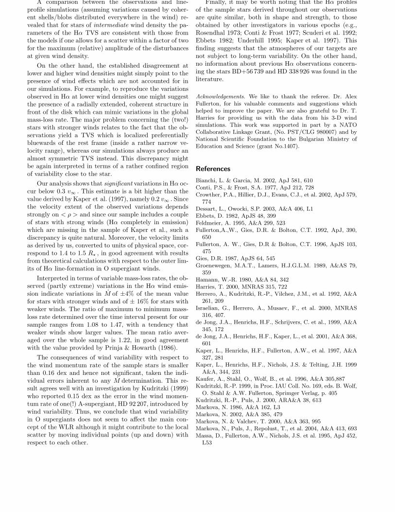
Markova et al.: Wind variability in O stars 21
A comparison between the observations and line-profile simulations (assuming variations caused by coher-ent shells/blobs distributed everywhere in the wind) re-vealed that for stars of intermediate wind density the pa-rameters of the Hα TVS are consistent with those fromthe models if one allows for a scatter within a factor of twofor the maximum (relative) amplitude of the disturbancesat given wind density.
On the other hand, the established disagreement atlower and higher wind densities might simply point to thepresence of wind effects which are not accounted for inour simulations. For example, to reproduce the variationsobserved in Hα at lower wind densities one might suggestthe presence of a radially extended, coherent structure infront of the disk which can mimic variations in the globalmass-loss rate. The major problem concerning the (two!)stars with stronger winds relates to the fact that the ob-servations yield a TVS which is localized preferentiallybluewards of the rest frame (inside a rather narrow ve-locity range), whereas our simulations always produce analmost symmetric TVS instead. This discrepancy mightbe again interpreted in terms of a rather confined regionof variability close to the star.
Our analysis shows that significant variations in Hα oc-cur below 0.3 v∞ . This estimate is a bit higher than thevalue derived by Kaper et al. (1997), namely 0.2 v∞ . Sincethe velocity extent of the observed variations dependsstrongly on < ρ > and since our sample includes a coupleof stars with strong winds (Hα completely in emission)which are missing in the sample of Kaper et al., such adiscrepancy is quite natural. Moreover, the velocity limitsas derived by us, converted to units of physical space, cor-respond to 1.4 to 1.5 R⋆ , in good agreement with resultsfrom theoretical calculations with respect to the outer lim-its of Hα line-formation in O supergiant winds.
Interpreted in terms of variable mass-loss rates, the ob-served (partly extreme) variations in the Hα wind emis-sion indicate variations in M of ±4% of the mean valuefor stars with stronger winds and of ± 16% for stars withweaker winds. The ratio of maximum to minimum mass-loss rate determined over the time interval present for oursample ranges from 1.08 to 1.47, with a tendency thatweaker winds show larger values. The mean ratio aver-aged over the whole sample is 1.22, in good agreementwith the value provided by Prinja & Howarth (1986).
The consequences of wind variability with respect tothe wind momentum rate of the sample stars is smallerthan 0.16 dex and hence not significant, taken the indi-vidual errors inherent to any M determination. This re-sult agrees well with an investigation by Kudritzki (1999)who reported 0.15 dex as the error in the wind momen-tum rate of one(!) A-supergiant, HD 92 207, introduced bywind variability. Thus, we conclude that wind variabilityin O supergiants does not seem to affect the main con-cept of the WLR although it might contribute to the localscatter by moving individual points (up and down) withrespect to each other.
Finally, it may be worth noting that the Hα profilesof the sample stars derived throughout our observationsare quite similar, both in shape and strength, to thoseobtained by other investigators in various epochs (e.g.,Rosendhal 1973; Conti & Frost 1977; Scuderi et al. 1992;Ebbets 1982; Underhill 1995; Kaper et al. 1997). Thisfinding suggests that the atmospheres of our targets arenot subject to long-term variability. On the other hand,no information about previous Hα observations concern-ing the stars BD+56739 and HD 338926 was found in theliterature.
Acknowledgements. We like to thank the referee. Dr. AlexFullerton, for his valuable comments and suggestions whichhelped to improve the paper. We are also grateful to Dr. T.Harries for providing us with the data from his 3-D windsimulations. This work was supported in part by a NATOCollaborative Linkage Grant, (No. PST/CLG 980007) and byNational Scientific Foundation to the Bulgarian Ministry ofEducation and Science (grant No.1407).
References
Bianchi, L. & Garcia, M. 2002, ApJ 581, 610Conti, P.S., & Frost, S.A. 1977, ApJ 212, 728Crowther, P.A., Hillier, D.J., Evans, C.J., et al. 2002, ApJ 579,
774Dessart, L., Owocki, S.P. 2003, A&A 406, L1Ebbets, D. 1982, ApJS 48, 399Feldmeier, A. 1995, A&A 299, 523Fullerton,A.,W., Gies, D.R. & Bolton, C.T. 1992, ApJ, 390,
650Fullerton, A. W., Gies, D.R & Bolton, C.T. 1996, ApJS 103,
475Gies, D.R. 1987, ApJS 64, 545Groenewegen, M.A.T., Lamers, H.J.G.L.M. 1989, A&AS 79,
359Hamann, W.-R. 1980, A&A 84, 342Harries, T. 2000, MNRAS 315, 722Herrero, A., Kudritzki, R.-P., Vilchez, J.M., et al. 1992, A&A
261, 209Israelian, G., Herrero, A., Musaev, F., et al. 2000, MNRAS
316, 407.de Jong, J.A., Henrichs, H.F., Schrijvers, C. et al., 1999, A&A
345, 172de Jong, J.A., Henrichs, H.F., Kaper, L., et al. 2001, A&A 368,
601Kaper, L., Henrichs, H.F., Fullerton, A.W., et al. 1997, A&A
327, 281Kaper, L., Henrichs, H.F., Nichols, J.S. & Telting, J.H. 1999
A&A, 344, 231Kaufer, A., Stahl, O., Wolf, B., et al. 1996, A&A 305,887Kudritzki, R.-P. 1999, in Proc. IAU Coll. No. 169, eds. B. Wolf,
O. Stahl & A.W. Fullerton, Sprimger Verlag, p. 405Kudritzki, R.-P., Puls, J. 2000, ARA&A 38, 613Markova, N. 1986, A&A 162, L3Markova, N. 2002, A&A 385, 479Markova, N. & Valchev, T. 2000, A&A 363, 995Markova, N., Puls, J., Repolust, T., et al. 2004, A&A 413, 693Massa, D., Fullerton, A.W., Nichols, J.S. et al. 1995, ApJ 452,
L53

22 Markova et al.: Wind variability in O stars
Meynet, G., Maeder, A., Schaller, G. et al. 1994, A&AS 103,97
Owocki, S.P. & Puls, J. 1999, ApJ 510, 355Owocki, S.P., Castor,J.I. & Rybicki, G.B. 1988, ApJ 335, 914Press, W.H., Flannery, B.P.,Teukolsky, S.A. et al. 1992,
Numerical Recipes: The Art of Scientific Computing (2ndedition), Cambridge: Cambridge Univ. Press, p. 634f.
Prinja, R.K. & Howarth, I.D. 1986, ApJS 61, 357Prinja, R.K. & Smith,L.J. 1992, A&A 266, 377Prinja, R.K. & Fullerton, A. 1994, ApJ, 426, 345Prinja, R.K., Balona,L.A., Bolton, C.T. et al. 1992, ApJ 390,
266Prinja, R.K., Fullerton, A.W. & Crowther, P.A. 1996, A&A
311, 264Prinja, R.K., Stahl, O., Kaufer, A. et al. 2001, A&A 367, 891Prinja, R.K., Massa, D. & Fullerton, A.W. 2002, A&A 388,
587Puls, J., Kudritzki, R.-P., Herrero, A., et al. 1996, A&A 305,
171Puls, J., Repolust, T., Hoffmann, T., et al. 2002, in Proc. IAU
Symp. No. 212, eds. K.A. van der Hucht, A. Herrero & C.Esteban, ASP Conf. Ser, p. 61
Rauw, G. , Morrison, N.D., Vreux, J.-M. et al. 2001, A&A 366,585
Repolust, T., Puls, J., Herrero, A. 2004, A&A 415, 349Rosendhal, J.F. 1973, ApJ 186, 909Scuderi, S., Bonanno, G. , Di Benedetto, R. et al. 1992, ApJ
392, 201Underhill, A.B., 1995, ApJS 100, 433Vink, J.S., de Koter, A., Lamers, H.J.G.L.M. 2000, A&A 362,
295Walborn, N. R. 1973, AJ, 78. 1067