Bridging the gap from ocean models to population...

Progress in Oceanography 84 (2010) 69–84

Contents lists available at ScienceDirect

Progress in Oceanography

journal homepage: www.elsevier .com/ locate /pocean

Bridging the gap from ocean models to population dynamics of large marinepredators: A model of mid-trophic functional groups

Patrick Lehodey a,*, Raghu Murtugudde b, Inna Senina a

a MEMMS (Marine Ecosystems Modeling and Monitoring by Satellites), CLS, Space Oceanography Division, 8-10 rue Hermes, 31520 Ramonville, Franceb ESSIC, Earth Science System Interdisciplinary Center, University of Maryland, USA

a r t i c l e i n f o

Article history:Available online 17 September 2009

0079-6611/$ - see front matter � 2009 Elsevier Ltd. Adoi:10.1016/j.pocean.2009.09.008

* Corresponding author. Tel.: +33 561 393 770; faxE-mail address: [email protected] (P. Lehodey).

a b s t r a c t

The modeling of mid-trophic organisms of the pelagic ecosystem is a critical step in linking the coupledphysical–biogeochemical models to population dynamics of large pelagic predators. Here, we provide anexample of a modeling approach with definitions of several pelagic mid-trophic functional groups. Thisapplication includes six different groups characterized by their vertical behavior, i.e., occurrence of dielmigration between epipelagic, mesopelagic and bathypelagic layers. Parameterization of the dynamics ofthese components is based on a temperature-linked time development relationship. Estimated parametersof this relationship are close to those predicted by a model based on a theoretical description of the alloca-tion of metabolic energy at the cellular level, and that predicts a species metabolic rate in terms of its bodymass and temperature. Then, a simple energy transfer from primary production is used, justified by the exis-tence of constant slopes in log–log biomass size spectrum relationships. Recruitment, ageing, mortality andpassive transport with horizontal currents, taking into account vertical behavior of organisms, are modeledby a system of advection–diffusion-reaction equations. Temperature and currents averaged in each verticallayer are provided independently by an Ocean General Circulation Model and used to drive the mid-trophiclevel (MTL) model. Simulation outputs are presented for the tropical Pacific Ocean to illustrate how differenttemperature and oceanic circulation conditions result in spatial and temporal lags between regions of highprimary production and regions of aggregation of mid-trophic biomass. Predicted biomasses are comparedagainst available data. Data requirements to evaluate outputs of these types of models are discussed, as wellas the prospects that they offer both for ecosystem models of lower and upper trophic levels.

� 2009 Elsevier Ltd. All rights reserved.

1. Introduction

The level of information, both in terms of understanding andobservations, for the physical and biogeochemical components ofthe pelagic ecosystem is now sufficient to make realistic basin-scale simulations of ocean physics and lower trophic (phytoplank-ton) level biology. On the other hand, the information is still verylimited for the intermediate or mid-trophic levels (micronekton).Yet, the modeling of these components is essential for understand-ing the dynamics of their predators that are most often heavilyexploited species. Pressing management issues require rapiddevelopments in understanding and prediction of the changesoccurring in these populations under the pressures of both fishingand climate change. Thus, it is a primary condition to develop anew generation of ecosystem models for the study and manage-ment of these exploited marine resources whose exploitation at-tracts increasing concerns on their sustainability or even a risk ofextinction in some cases.

ll rights reserved.

: +33 561 393 782.

Given these pressing issues, the modeling approach certainlyrequires realism and pragmatism, especially if we use ‘‘ecosystem”in its whole sense that is including both the physical environmentand the set of all living organisms and their interactions in spaceand time, with each other and with their environment. There isan obvious huge gap between the recent achievements in physicaloceanography, with the development of ocean general circulationmodels (OGCMs), and our capacity to model the incredible com-plexity of the marine life. Though less advanced in understandingand representation of underlying mechanisms, the new generationof biogeochemical models (BGCM) appears also mature enough tocapture the global features (spatio-temporal, seasonal-to-interan-nual and multi-decadal variability) of the components of the car-bon cycle. Of course, there is still a vast field of research forincluding increasing complexity of processes, in particular overthe continental slopes, shelf-breaks, and coastal areas, but at leastthere is a simplified and coherent vision of these biogeochemicalcomponents, and the coupling between OGCM and BGCM(OGCBM) is now a common practice. In addition, for both typesof models, there exist synoptic (satellite-derived) and in situ obser-vations allowing model evaluation and data assimilation.

http://dx.doi.org/10.1016/j.pocean.2009.09.008

mailto:[email protected]

http://www.sciencedirect.com/science/journal/00796611

http://www.elsevier.com/locate/pocean

70 P. Lehodey et al. / Progress in Oceanography 84 (2010) 69–84

The situation is remarkably different as soon as we move up astep in this great ecosystem picture, i.e. for zooplankton and moreparticularly the mid-trophic levels that constitute forage organ-isms of predator species; the latter being frequently exploited mar-ine resources. The challenge proposed here is to model thesecomponents of the marine ecosystem despite the very limitedknowledge and observation available, thus using an approach assimple as possible, but that can be coupled nonetheless, to theother components (OGCBM) without loosing the benefit of the bet-ter insights and detailed modeling possibility they offer. Thismeans that the new modeled components have to be spatially-ex-plicit and at least constrained by their bio-physical environmentpredicted by the OGCBM, if not fully coupled to investigate poten-tial biological feedbacks.

Given the diversity of species and interactions in the food webstructure, the approaches for modeling ecosystem ecology relymainly on the energetic view as stated by Lindeman (1942),describing the ecosystem as a flow of energy through a networkfrom the first trophic level (primary producers) to the consumersgroups. The question is how to define these groups. In its simplestexpression, it would be a chain of discrete trophic levels, as in atrophic pyramid. The concept then can be extended to a largernumber of groups producing an increasingly complex networkwith potential interactions between one group and all the others,and requiring the introduction of a continuous representation oftrophic levels.

This approach of trophic flow models has been proposed andused for investigating different marine ecosystems (Christensenand Pauly, 1992) but it becomes limited by the extensive numberof parameters exponentially increasing with the number of groupsdefined to represent the network. The parameterization of the tro-phic network in such models becomes an unrealistic static viewwhen considering the plasticity of organisms and their aptitudeto switch from one prey (or group of prey) to another. Besides,most of oceanic large predators are opportunistic feeders with avery large spectrum of prey species. In addition, the definition ofgroups by trophic levels may be problematic since organisms canoccupy many different trophic levels over their life.

A second approach is then to consider the size spectrum in theecosystem. The size was effectively identified as a fundamental cri-terion that structures the ecosystem, especially the marine ecosys-tem. The size of an organism largely determines its function in theecosystem: it controls the diet based (roughly) on prey–predatorsize relationships; there is an obvious size-abundance relationship,the smaller organisms being the most abundant (Elton, 1927); andfinally metabolism and turnover also appear linked to it. These lat-ter relationships have been investigated for long and seen in multi-ple empirical observations. Kleiber (1932) was the first to provide asurprising result by showing that an animal’s metabolic rate is pro-portional to its body mass raised to the power of 3=4. Since then, scal-ing laws based on exponents in which the denominator is amultiple of four have been proposed in various ways. Empirical dataalso suggest allometric relationships between abundance per unitarea and body size (or weight) both in terrestrial and marine sys-tems (e.g., Sheldon et al., 1972; Kerr, 1974; Enquist et al., 1998; Bel-grano et al., 2002), or similarly between weight of organisms andthe growth rate of their population (Fenchel, 1974; Savage et al.,2004). It follows from these findings that abundance at a given size(weight) or ‘‘size window” is constrained by rates of energy supply,thus leading to macroecological properties. Therefore, abundanceor biomass-body size (weight) relationships have been used to de-scribe the energy flow in biomass size spectrum in different ecosys-tems which interestingly showed similar slopes in log–logrelationships (Dickie, 1976; Boudreau and Dickie, 1992).

Underlying mechanisms that can explain these scaling laws areobviously of critical significance for ecological modeling. Platt and

Denman (1978) proposed a first attempt to understand the sizestructure of pelagic ecosystems under energetic balances. Theydemonstrated that ‘‘the trophic structure of an ecosystem is con-trolled in some way by the magnitudes of various physiological ratesof the component organisms” (Platt, 1985), thus establishing theallometric basis that structures the marine ecosystems. More re-cently, a theory known as the Metabolic Theory of Ecology (MTE)has been proposed by Brown et al. (2004) to describe how the met-abolic rate of individual organisms varies with body mass and tem-perature. Another approach proposed previously by Kooijman(1986) was based on a model of dynamics energy budget (DEB).Though based on similar principles (e.g., the van Hoff-Arrheniusequation), the approaches are different and debated (Van der Meer,2006), and will require much work and experimentation beforeproviding the kind of unifying conceptual frameworks needed formodeling the ecosystem based on molecular principles.

Nevertheless, scaling laws like allometric relationships are nowsufficiently well established to be used as a practical modeling ap-proach especially since critical issues like climate change or man-agement of (over) exploited marine species require the rapiddevelopment (e.g., in the coming 5–10 years) of ‘‘Minimum Realis-tic Models” (MRM) as defined by Butterworth and Plaganyi (2004),i.e. ‘‘with the underlying concept to restrict the model developed tothose species most likely to have important interactions with the spe-cies of interest”.

In this paper, one pathway is presented as an alternative to thesize spectrum approach that combines energetic and functional ap-proaches, to model the mid-trophic level organisms of marine eco-systems. Instead of describing the full size spectrum of the marineecosystem, we propose to model several functional groups for a gi-ven size or weight window, corresponding to the biomass of forageorganisms of large oceanic predators, i.e. roughly the micronekton.Rather than considering size, this approach is based on the temper-ature-linked development time of the organisms and the turnoverof their multi-species population functional groups. The bio-phys-ical forcing provided by one OGCBM is used to produce a simula-tion of the mid-trophic functional components. Then the interestof representing these new functional groups as a link for investi-gating and modeling the dynamics of fish populations is discussed.

2. Modelling approach

2.1. Conceptual model of the mid-trophic functional groups

Oceanic micronekton includes a myriad of species providingforage for larger predators. They can be roughly characterized bya size spectrum in the range of 2–20 cm dominated by crustaceans,fish, and cephalopods. Gelatinous organisms like jellyfish are alsolikely an underestimated important component of micronektonin the functioning of the system but apparently have a limitednumber of predators. One distinctive characteristic of most of theseorganisms is to perform diel vertical migrations, moving betweendeep layers during the day to the surface layer at night. This evo-lutionary adaptation likely decreases the predation pressure dur-ing the day in the upper layer though predators also haveadapted their behavior under the same constraints, i.e. finding foodand avoiding bigger predators. But the essential result is that theflow of energy generated by autotrophic organisms in the euphoticlayer is transferred to the deeper meso- and bathy-pelagic layersthrough these daily migrations. Acoustic and micronekton sam-pling studies indicate that most of the micronekton biomass occu-pies the meso- and bathy-pelagic layer. Therefore, according toLegand et al. (1972), and Grandperrin (1975), about 90% of the bio-mass of macroplankton and micronekton in the tropical PacificOcean is typically concentrated in the 0–500 m upper layer during

P. Lehodey et al. / Progress in Oceanography 84 (2010) 69–84 71

the night and 50% in the 0–100 m layer, however, only 10% remainsin the first 200 m during the day. Similarly, Hidaka et al. (2003)found a factor 10 between day and night biomass of micronektonin the upper 200 m of the western tropical Pacific Ocean. Predatorsof these mid-trophic organisms have evolved to prey upon thesespecies, i.e., either they chase the prey species migrating in thelayer they inhabit, or they make temporary excursions in the layerswhere these species remain. Through evolution, the predators havethus developed sensory, morphological and physiological adapta-tions allowing them to exploit cold, dark and sometimes oxygendepleted deep layers. Hence, vertical movements appear to be akey process in structuring the ocean ecosystem, and therefore anessential mechanism that has to be accounted for when designinga functional view of the system.

Following this idea, and based on existing knowledge (c.f. a re-view in Appendix A), a simple conceptual model of the mid-trophiclevel components can be proposed with six functional groups inthree vertical layers: epipelagic, mesopelagic and bathypelagic(Fig. 1). The pelagic micronekton is divided into epipelagic, meso-pelagic and bathypelagic groups, the last two groups subdividedinto vertically migrant and non-migrant species. Since light inten-sity is likely a major factor that controls diel vertical migrations ofmeso- and bathy-pelagic organisms, the euphotic depth is a logicaland convenient way to define the vertical boundaries of the threelayers. Preliminary examinations of predicted euphotic depthsfrom biogeochemical models indicate that using the euphoticdepth as the boundary for the epipelagic layer and defining theboundary between meso- and bathy-pelagic layers by three timesthe euphotic depth would produce values similar to those definedfrom biological observations, e.g., between 50 and 150 m for epipe-lagic and 150 and 450 m for mesopelagic layers in the eastern andwestern tropical Pacific Ocean respectively.

2.2. Spatio-temporal dynamics of functional groups

Here, micronekton functional groups are considered as singlepopulations composed of different species, and then modeledusing the same equations as for single population model (see pre-vious references in Lehodey et al., 1998; Lehodey, 2001), with con-tinuous mortality and recruitment (e.g., Ricker, 1975). Instead ofhaving different age classes (cohorts) of the same species, thereare different age classes of many different species, the mathemat-ical solution being the same (Allen, 1971).

The concept of this model dynamics was illustrated as follows(Lehodey, 2004a): ‘‘at any time, anywhere in the ocean, there is amixing of all kinds of eggs, cells, etc. that are the germs of the fu-ture organisms of the pelagic food web. In some places and at some

EDay Length (DL) as a function of

latitude and date

E’n

day

night sunset, sunrise

Epipelagic layer

surface1 2 3 4 5 6

Mesopelagic layer

Bathy pelagic layer

PP

Fig. 1. Conceptual model of the mid-trophic components in the pelagic ecosystem.Daily vertical distribution patterns of the micronekton in the pelagic ecosystem: (1)epipelagic; (2) migrant mesopelagic; (3) non-migrant mesopelagic; (4) migrantbathy-pelagic; (5) highly migrant bathypelagic; and (6) non-migrant bathypelagic.The part of energy (E) transferred from primary production (PP) to intermediatetrophic levels is redistributed (E0n) through the different components.

times, the input of nutrients into the euphotic zone allows an al-most immediate development of phytoplankton (primary produc-tion P) that is the input source into the forage population model (F).This new production allows the development of a new ‘‘cohort” oforganisms, i.e., true zooplankton like copepods as well as all larvaeof fish and other larger organisms (meroplankton). The organismshaving a longer lifespan and a larger growth potential (larvae andjuvenile of fish, squids, shrimps, etc.) feed at the expense of theorganisms with a shorter lifespan and a lower growth potential(phytoplankton, zooplankton). As the water masses are maturing,they are advected with these organisms (but a part of them canalso diffuse away due to the diffusion of water and their own ran-dom movements) and the currents create fronts of convergencewhere forage is aggregated. Of course these dynamics occur as acontinuous process in time and space. Following this time-trophiccontinuum concept, the species [for a given cohort] should disap-pear selectively in the order of their trophic level related to theirtime of development”. At the time (tr) they are entering(�recruited in) the forage population F (biomass), the survivalorganisms – the amount of which is linked to the energy efficiencycoefficient E – provide the forage production (F0).

In this approach there is no size structure in functional groupsbut accumulation of biomass (after a given recruitment time tr)through an energy efficiency coefficient E with primary produc-tion as the source. However, these functional groups can be con-sidered as body size ‘‘windows” of the full size spectrum of themarine system. Given the lack of detailed information concerningthe consumption rates and the links between zooplankton andmicronekton groups, it was in fact an easy and feasible way atthis stage to implement ecological transfer from primary produc-tion to micronekton groups (see Appendix B). This representationappears sufficient for developing new modeling approaches andapplications to population dynamics of exploited species (see Sec-tion 5).

The spatial dynamics are considered and described with anadvection–diffusion equation using horizontal currents for theadvective terms and a diffusion coefficient (q = 10,000 m2 s�1)incorporating both diffusion of water and random movement oforganisms. During the time that a mid-trophic functional groupis occupying its day or night layer, it is transported by the cur-rents averaged through corresponding layers. The time spent inone or the other layer is calculated from the day length equationas a function of the latitude and the Julian day (see Appendix C).

2.3. Parameterization of the turnover of the functional groups

The turnover of mid-trophic functional groups is controlled bythe parameter k (mortality coefficient) and the parameter tr thatis the minimum age to be recruited in the mid-trophic functionalpopulation. The maximum lifespan defined as the time necessaryto see the population reduced to a determined level (e.g., x = 1%or 5%) is tmax = �1/k Ln(x) + tr (Lehodey, 2001). The turnover of apopulation is usually defined as the generation time or the averageage at maturity tm of the individuals in the population, hence it isuseful to search for a relation between age at maturity and themean age of population that could help in the parameterizationof k. Indeed, age at maturity and lifespan are important criteriain population dynamics and it has been empirically demonstratedin a study by Froese and Binohlan (2000) that they are both linkedfollowing a log–log linear relationship (Eq. (1)).

logðtmaxÞ ¼ 0:5496þ 0:957 logðtmÞ ð1Þ

By substituting tmax by its definition above, we obtain equation:

t0:957m ¼ � lnðxÞ

100:5496 � kþ 1

100:5496 � tr ð2Þ

y = -0.1252x + 7.6541R2 = 0.8834

0123456789

0 4 8 12 16 20 24 28

Tc / (1+ (Tc/273))

Ln(t m

)

CephalopodCrustaceanFish

0

300

600

900

1200

1500

1800

2100

2400

Tc (°C)

t d (d

ay)

0

300

600

900

1200

1500

1800

2100

2400

0 4 8 12 16 20 24 28 32

Tc / (1+ (Tc/273))

t d (d

ay)

1/ λ

t m = 1/3 tr + 1/ λ

t r = 1/4 t m

Fig. 2. Age at maturity of species (tm) in relation to their average habitattemperature (ambient temperature Tc). Observations derived from the literatureare used to estimate the coefficients of the exponential decreasing functionspredicting the turnover of mid-trophic groups (see text for explanation). Coeffi-cients are estimated from a log-linear regression. For each Class of species,observations are sorted by decreasing average habitat temperature. Cephalopods:Bathypolypus arcticus1, Octopus doeini1, Illex illecebrosus1, Loligo vulgaris1, Loligoforbesi1, Loligo opalescens1, Sepioteuthis lessoniana1, Ommastrephes bartramii4,Euprymna scolopes1, Idiosepius pygmaeus1, Sepioteuthis lessoniana2, Sepioteuthislessoniana3, Loliolus noctiluca5, Loligo chinensis5, Idiodepius pygmaeus5, Sepiellainermis1, Sepioteuthis lessoniana1. Crustaceans: Pandalus borealis6, Pandalus borealis6,Pandalus borealis6, Pandalus borealis6, Pandalus borealis6, Metherytrops micropht-alma7, Pandalus borealis6, Pandalus borealis6, Euphausia superba8, Pandalus borealis6,Euphausia pacifica8, Thysanopoda tricuspidata9, T. monocantha9, T. aequalis9, Nema-toscelis tenella9, Euphausia diomedae9, Euphausia eximia8, Nycthiphanes simplex8. Fish:Mallotus villosus10, Leuroglossus schmidti11, Stenobrachius leucopsarus11, Clupeaharrengus12, Clupea pallasi13, Clupea harrengus14, Engraulis encrasicolus15, Sardinopsmelanostictus16, Scomber japonicus17, Engraulis capensis18, Engraulis encrasicolus19,Engraulis ringens18, Sardinops sagax18, Engraulis mordax18, Engraulis japonicus20,Vinciguerria Nimbarria21, Encrasicholina punctifer22. References: 1Wood and O’Dor(2000); 2Jackson and Moltschaniwskyj (2002); 3Forsythe et al. (2001); 4Ichii et al.(2004); 5Jackson and Choat (1992); 6Hansen and Aschan (2000); 7Ikeda (1992);8Siegel (2000); 9Roger (1971); 10Carscadden et al. (1997); 11Abookire et al. (2002);12Alheit and Hagen (1997); 13Hunter and Wada (1993); 14Reid et al. (1999);15Samsun et al. (2004); 16Hunter and Wada (1993); 17Prager and MacCall (1988);18Schwartzlose et al. (1999); 19Allain (2005); 20Takahashi and Watanabe (2004);21Stéquert et al. (2003); 22Dalzell (1993).


Given the range of standard error of the original regression (Fro-ese and Binohlan, 2000), and taking x = 0.05, Eq. (2) can be simpli-fied into Eq. (3):

tm ¼ 1=kþ 1=3 tr ð3Þ

As useful as this relationship can be, it would be more satisfyingto deduce a formal relationship between mortality k and tm from atheoretical basis. The dynamic energy budget (Kooijman, 1986) orthe Metabolic Theory of Ecology (Brown et al., 2004) may offersuch a theoretical framework. At the population level, turnover islinked to biological rates of individual organisms and then relieson the metabolic rates at which these organisms use and transformenergy and materials (e.g., Platt, 1985; Savage et al., 2004). Theserates obey the thermodynamic laws, i.e., the physical and chemicalprinciples that govern the transformation of energy and materials,and while the metabolism is linked to the size of organisms, thetime needed to reach a given size (weight) is constrained by theambient temperature.

Gillooly et al. (2002), following the work of West et al. (1997,2001), describe the allocation of metabolic energy at the cellularlevel, having developed a model that predicts a linear relationshipbetween the natural logarithm of a mass-corrected developmenttime (t/m1/4) and the ambient temperature at which the develop-ment stage occurs (Tc in �C), or to be more precise, the term Tc/(1 + (Tc/273)). They illustrated the capacity of the model to predicthow size and temperature affect embryonic development time ofaquatic ectotherms (fish, amphibians, aquatic insects, and zoo-plankton) and birds, as well as the post-embryonic to maturitydevelopment time of zooplankton species. Their model predictsapproximately universal straight line with the slope, a ¼ �E=kT2

0

with E the activation energy for metabolic reactions, k the Boltz-mann’s constant and T0 = 273 K. Because both the slope and inter-cept depend on fundamental cellular properties, they do not varysignificantly across taxa. With E = 0.6 eV (an average of the ob-served range 0.2–1.2 eV), the model predicts a = �0.09 per �C,while values obtained by regression from different data sets arein the range of �(0.11–0.14) (Gillooly et al., 2002).

Similarly, we have investigated the relationship between age atmaturity of mid-trophic species and their ambient temperature.Unfortunately it is very difficult to obtain from the literature thethree variables needed, i.e. the age at maturity tm, the body mass atmaturity m and the ambient temperature Tc. We were able howeverto compile a dataset of tm and Tc for mid-trophic species of the maintaxa of ocean mid-trophic groups, i.e., crustaceans, fish and squid.Parameters were estimated from a log-linear regression (Eq. (4);Fig. 2) that gives a good fit to the data (Nobs = 45; R2 = 0.889).

LnðtmÞ ¼ 7:654� 0:125ðTc=ð1þ ðTc=273ÞÞÞ ð4Þ

To be fully comparable with the model proposed by Gillooly andco-authors, observations of time of development to age at maturityfor these species (Fig. 2) should be also corrected relatively to themass factor (m1/4). Nevertheless, it is clear that these results sug-gest that Gillooly et al.,’s model could be effectively extended tothese other taxa, at least concerning the development time untilthe onset of maturity during which the energy is devoted togrowth and somatic maintenance only. The slope (�0.125) andthe intercept (7.654) that we obtained are in the range of whathas been obtained with other datasets (Gillooly et al., 2002).

Finally, substituting 1/k + 1/3 tr for tm into Eq. (4), we obtain aparameterization of k linked to the ambient temperature and tr

(Fig. 2). The parameterization of tr itself would require a detailedstudy to compile a dataset of time of development, i.e., age, andambient temperature for organisms to reach the minimum size ofthe modeled mid-trophic functional groups. Indeed, a relationshipof temperature-linked time of development to reach a minimumweight would be more accurate. On the basis of a few observations

from tuna diets, we have fixed to 1 g the minimum weight of themid-trophic groups, e.g., this is the average weight of pelagic crabmegalopa that are eaten in large number by yellowfin tuna off east-ern Australia (J. Young, personal communications, CSIRO). Marineorganisms reach this minimum weight in much less than 1 monthin warm waters (>28 �C); a good example is given by tuna larvae thatcan reach 5 cm after only 1 month in the Pacific warm pool. In colderwater (10–15 �C) like in the upwelling systems of the Humboldt, Cal-ifornia or Benguela, growth studies of anchovy, sardines and otherClupeidae suggest a value of tr above 2 months (Palomares et al.,1987). Finally in very cold water (<5 �C) it may require more than10 months to reach this minimum weight. In sub-antarctic waters(2–5 �C) for example, pteropods, a small but important prey species


of Pacific salmon, is adult after 1 year (Kobayashi, 1974). Since thereis no reason to have a different slope in the temperature relationshipfor tr, we used tr = 1/4 tm to match these very scarce observations(Fig. 2). This simple definition leads to a maximum value of2109 days and 527 days for 1/k and tr respectively at Tc = 0 �C andthe same exponential coefficient (�0.125).

3. Model configuration and forcing data set

The model domain covers the Pacific Ocean with a grid extend-ing from 65�N to 50�S at 1� �month resolution. To drive the inter-mediate trophic functional groups, we used physical andbiogeochemical forcing data sets derived from a coupled physi-cal–biogeochemical model.

The Ocean General Circulation Model (OGCM) is based on a re-duced gravity, primitive equation, r-coordinate model coupled toan advective atmospheric mixed layer model (Murtugudde et al.,1996). Numerous studies on tropical ocean variability, tropical-subtropical interactions, physical–biological feedbacks, and cou-pled ecosystem variability have been reported demonstrating themodel’s ability to capture the sub-seasonal to interannual variabil-ity of the dynamics and thermodynamics in the tropics (e.g., Chenet al., 1994; Murtugudde et al., 2002, 2004).

A biogeochemical model has been fully coupled to the OGCM de-scribed above and tested in the three tropical oceans (Christian et al.,2002; Christian and Murtugudde, 2003; Wiggert et al., 2006). Thismodel consists of nine components: two size-classes each (largeand small) of phytoplankton, zooplankton and detritus, and threenutrient pools: ammonium, nitrate, and iron. The incorporation ofiron into the ecosystem model is of vital importance for improvingthe prediction of the ecosystem response as iron has been identified

Fig. 3. Comparison between observed (top) chlorophyll concentration (CZCS satellite) andand El Niño phases in the western equatorial Pacific (September 1981 and December 19

as an important element controlling phytoplankton growth and bio-mass in large regions of the world’s oceans (Coale et al., 1996; Mar-tin, 1990; Martin et al., 1994). This model works well in reproducingecosystem dynamics and biogeochemical fields at seasonal to inter-annual time scales (Wang et al., 2005, 2006a,b), though the variabil-ity of primary production is underestimated, a tendency observed inall biogeochemical models (R. Feely, 2005, personal communica-tions). Figs. 3 and 4 illustrate the ability of the model to capturethe interannual and decadal variability in the primary productionin the tropical, extra-tropical, and mid-latitude regions.

For simplicity in this first application, temperature and horizon-tal current variables were averaged in three vertical layers (seeAppendix C for details), with fixed depths rather than based on var-iable euphotic depths: epipelagic (0–100 m), mesopelagic (100–400 m) and bathypelagic (400–1000 m). The primary productionwas integrated through 0–400 m. The period of simulationspanned 1948–2004 period. A monthly climatology was createdfor all forcing variables as a monthly means computed over allyears of simulation, and used for the spin-up to build up the bio-mass of the different functional groups and to reach equilibrium,i.e., practically, after a number of time steps P (tr,max + 1/kmax).Though the simulation domain covered the full Pacific basin, wewill focus our analysis on the tropical (30�N–30�S) region.

4. Results

4.1. Simulation outputs

The distribution in the epipelagic layer during the day is themost contrasted, due to higher temperature (faster turnover) andstronger environmental variability in this layer than in the deeper

predicted primary production (ESSIC NPZD model, mmol C m�2 d�1) during La Niña82 respectively).

-3

-2

-1

0

1

2

J-48

J-54

J-60

J-66

J-72

J-78

J-84

J-90

J-96

J-02

SOI

405060708090100110120

PP

SOI EEP

-3

-2

-1

0

1

2

J-48

J-54

J-60

J-66

J-72

J-78

J-84

J-90

J-96

J-02

SOI (

reve

rsed

axi

s)

10

20

30

40

50

60

70

PP

SOI FWP

-3

-2

-1

0

1

2

3

J-48

J-54

J-60

J-66

J-72

J-78

J-84

J-90

J-96

J-02

PDO

0

20

40

60

80

100

120

PP

PDO KUREX-3

-2

-1

0

1

2

3

J-48

J-54

J-60

J-66

J-72

J-78

J-84

J-90

J-96

J-02

PDO

20

25

30

35

40

45

50

PP

PDO GOA

Fig. 4. Predicted time series of average total primary production (black curves, in mmol C m�2 d�1) in four different geographical boxes superimposed over the southernOscillation or the Pacific Decadal oscillation indices (SOI and PDO respectively, grey shaded curves). EEP: Eastern equatorial Pacific, 10�N–10�S; 140�W–100�W. FWP: FarWestern Pacific, 15�N–5�S; 125�E–160�E. KUREX: Kuroshio Extension, 40�N–30�N; 140�E–170�E. GOA: Gulf of Alaska, 62�N–50�N;160�W–130�W.


layers. On average, there is a latitudinal shift of maximum concen-tration that appears in the equatorial region on each side of theequator (Fig. 5). The maximum of biomass in the surface layer dur-ing the day occurs in the eastern Pacific in association with thecoastal Peruvian upwelling and in the west in the shallow watersof the Papua New Guinea-Indonesia and Philippine waters, wherein addition to high primary productivity levels, most of the energyis transferred to the upper layer since there are no bathy- andmeso-pelagic layers. When comparing the biomass distributionin the different layers, there is an obvious contrast between foragebiomass in the epi- and bathy-pelagic layers during the day (Fig. 5),most of the biomass being concentrated in the deepest layer(Fig. 6). The average spatial distribution of bathypelagic biomassis more diffuse with a contrast between a rich cold-tongue associ-ated with the equatorial upwelling and merging in the east withthe highly productive coastal upwelling along the Peruvian coastand lower biomass on each side in the central gyres.

The contrasts in spatial distribution are also associated withtime lags in the turnover of the mid-trophic components. Forexample, low and high peaks in primary production are propagatedwith a delay of �2 months in the epipelagic component in theequatorial east Pacific, but because of the cold temperature inthe deep layer, the lag increases to 12–14 months for the bathype-lagic group (Fig. 5). These differences can lead to opposite peaks inthe fluctuation of epipelagic and bathypelagic groups (Fig. 5) andcomplex spatial heterogeneity due to redistribution by oceaniccirculation.

In addition to their own internal dynamics, the mid-trophic com-ponents are affected by the interannual and longer time scale vari-ability of climate and the environment, through changes intemperature, currents and primary production. These changes arereproduced by the physical–biogeochemical model (Fig. 4) and theeffects on mid-trophic components illustrated in Fig. 6, where bio-mass time series of the six mid-trophic components are providedfor the equatorial box 5�N–5�S; 120�W–100�W. With different timelags, all components are affected by ENSO-related interannualvariability (e.g. El Niño events of 1972–1973, 1982–1983 and1997–1998, and La Niña events of 1988–1989 and 1999–2000).The amplitude of ENSO-related fluctuations decreases through the

mid-trophic groups in relation with the proportion of time spent inthe upper layers, i.e. that groups with higher turnovers and low bio-mass over production ratio are more affected than groups with lowerturnovers and high B/P ratios (Fig. 6). Considering all the mid-trophicgroups together, the sum of their anomalies relatively to the meanbiomass of each group is correlated to the Southern Oscillation Index(SOI) with a maximum coefficient of correlation (r = 0.64) for a timelag of 6 months. Interestingly, frequency of the ENSO signal issmoothed through the different mid-trophic groups, leading to dec-adal periods dominated by positive (1950–1977) or negative (1978–1999) anomalies, the last one being positive and starting in 2000.This cascade of ENSO influences through the mid-trophic levelsneeds further validation against observations even though thereare only sparse observations.

On the spatial scale, the ENSO variability, characterized by largechanges in surface circulation, temperature distribution and pri-mary production (Fig. 3), strongly affects the forage biomass distri-bution in the tropical regions (Fig. 7). For example, at the end of thelast strong El Niño event of 1997–1998, the simulation predicts aninteresting asymmetric distribution of epipelagic biomass relativeto the equator with an enhanced biomass west of the Dateline,and conversely a more strongly depleted southern subtropicalgyre. This pattern is observed both for day and night distributions(Fig. 7) with in addition a substantial increase of biomass at nightin the eastern Pacific Ocean. At night, the biomass in the upperlayer increases by a factor 6–10 due to migration of meso- andbathy-pelagic components (Fig. 7).

4.2. Evaluation

Despite the wide spatio-temporal distribution and huge abun-dance of mid-trophic level organisms and their major influenceon top predator distribution and population dynamics, they arestill one of the less known components of pelagic ecosystems.The first source of observation that can be used for the parameter-ization of the model and the evaluation of its outputs are biomassestimates from different micronekton sampling cruises. Becausetime and cost constraints, as well as difficulty inherent to net sam-pling techniques (e.g. to collect the most agile organisms such as

80

100

120

140

160

J-66

J-66

J-67

J-67

J-68

J-68

J-69

J-69

J-70

J-70

J-71

J-71

J-72

J-72

Prim

ary

prod

.

0.2

0.3

0.4

Epip

elag

ic b

iom

PP epi

80

100

120

140

160

J-66

J-66

J-67

J-67

J-68

J-68

J-69

J-69

J-70

J-70

J-71

J-71

J-72

J-72

Prim

ary

prod

.

3.0

3.2

3.4

3.6Ba

thyp

elag

ic b

iom

PP bathy

Fig. 5. Average spatial distribution over all the time series (1948–2004) of purely epipelagic (a) and bathypelagic (b) groups. Due to difference in the habitat temperatures,turnover rates of mid-trophic populations are different. The average biomass time series of epipelagic (c) and bathypelagic (d) components for the box 5�N–5�S; 120�W–100�W (identified on the maps) indicate a lag with primary production of about 2 months for epipelagic group and 12–14 months for bathypelagic group. Primary productionis in mmol C m�2 d�1 and biomass unit for mid-trophic groups in g WW m�2.


squids), these sparse observations provide only part of the picture.Nevertheless, they are essential data providing a first order esti-mate of the absolute biomass of micronekton in the water column.For example, the EASTROPAC cruises in 1967–1968 (Blackburn andLaurs, 1972) provided distributions of micronekton in the easternequatorial Pacific Ocean (EPO) in the upper 200 m showing anincrease in biomass between day and night from �1–8 to10–20 ml/1000 m3, and still some higher concentration near thecoast of Peru. Assuming a conversion of 1 g per ml and since theepipelagic layer here is 100 m, this leads to value of 0.1–0.8 and1–2 g WW m�2 for day and night respectively, which is consistentwith the model outputs (Fig. 7).

On the other side of the basin, Hidaka et al. (2003) sampled in thewarm pool, north of Papua New Guinea (0�N–10�N; 140�E–150�E)during a cruise in January–February 1998. They calculated that the

micronekton biomass in the upper 200 m was in general<1 mg WW m�3 (0.01–0.7 mg WW m�3) during the day, with afew exception when large schools of epipelagic anchovy wereencountered (max. value 23.3 mg WW m�3), and increased to arange of 3–38.8 mg WW m�3 at night. Here, after converting tog WW m�2 for a 100 m epipelagic layer (i.e., multiplying by 100 mand dividing by 1000 mg), we obtain a range of 0.001–0.07 and0.3–3.88 g WW m�2 for day and night respectively that are in thesame order of predicted values as shown on Fig. 7(a and b).

With the development of acoustic techniques and surveys, theuse of micronekton net sampling has become a useful method tocalibrate and standardize the biomass integration from the acous-tic signal. However, the simulated migrant pelagic biomass in-cludes all type of organisms while acoustic data frequently targetone group of species, e.g., mesopelagic fishes (McClatchie and

0123456789

10

J-48

J-52

J-56

J-60

J-64

J-68

J-72

J-76

J-80

J-84

J-88

J-92

J-96

J-00

J-04

Biom

ass

(g m

-2) epi

mmesomesohmbathymbathybathy

-2.5

-2.0

-1.5

-1.0

-0.5

0.0

0.5

1.0

1.5

J-48

J-51

J-54

J-57

J-60

J-63

J-66

J-69

J-72

J-75

J-78

J-81

J-84

J-87

J-90

J-93

J-96

J-99

J-02

Biom

ass

anom

aly

(g m

-2)

-4

-3

-2

-1

0

1

2

3

SOI

bathy mbathyhmbathy mesommeso epi

Fig. 6. Time series of total biomass (in g WW m�2) and anomaly in biomass (difference to the average of the time series) for the six mid-trophic functional groups predicted inthe box 5�N–5�S; 120�W–100�W (c.f. map in Fig. 5). Southern Oscillation Index (SOI) is superimposed (dotted line) on the anomaly time series.


Dunford, 2003). Thus, these surveys provide a useful but still roughevaluation and require careful calibration. Nonetheless, acousticstudies offer the considerable advantage of potentially providinglong time series of data. As an illustration of the interest of acousticmonitoring for model evaluation, we compared the backscatter sig-nal of ADCP (Acoustic Doppler Current Profiler) that was deployedon the TAO-TRITON array of oceanographic buoys at two locationson the Equator, at 165�E and 170�W, with primary production andbiomass of mid-trophic components in the epipelagic layer atnight, both predicted from the simulation above (Fig. 8). ADCPbackscatter signal is linked to the biomass of macrozooplankton(roughly >1 cm) and micronekton and thus is an abundance indexof the mid-trophic organisms. The comparison shows that fluctua-tions of the ADCP time series are delayed by approximately2 months relative to the predicted primary production. This is acoherent result given the expected delay between primary and sec-ondary/tertiary production. Conversely, these fluctuations matchvery well those of the predicted mid-trophic biomass suggestingthat the model captures the important spatio-temporal dynamicsof these groups.

We will continue, for the evaluation of the model outputs, tocompile more of these direct and indirect measures of mid-trophicbiomass. Furthermore, we will search for an approach to use longtime series of acoustic profiles to be processed and directly assim-ilated in the model for parameter optimisation. This will requireidentifying the functional groups in the echograms and to extractthe corresponding part of the signal.

5. Discussion

Organisms occupying the mid-trophic level either temporarilyor permanently during their life can be both prey of larger preda-tors but also predators of smaller organisms, including eggs, larvae

and small-size juveniles of marine pelagic species. Therefore, theycan potentially control the dynamics of all marine species throughdifferent mechanisms, which can produce complex results, wheninteracting in a dynamic system.

First, mid-trophic organisms are prey of large oceanic species thatare essentially opportunistic omnivorous predators. Most of theselarge predators are in the upper layer during the night, while duringthe day species have evolved to exploit different vertical layers. If weconsider the schematic view of the pelagic system with three verticallayers: epi-, meso- and bathy-pelagic, as used to describe the mid-trophic components in the present study, it is relatively easy toroughly classify different vertical behavior types of top predatorsaccording to their ability to explore the deeper layers. Thus, bothhorizontal and vertical distributions of prey fields are certainly keyfactors to understand the spatio-temporal dynamics of the large oce-anic predator species, and the modelling approach presented hereoffers an ideal framework for developing new generation of spa-tially-explicit population dynamic models of exploited oceanic pre-dators of micronekton.

One example of coupling a fish population dynamic model tothis suite of models representing ocean physics to lower andmid-trophic levels is the spatial ecosystem and populationsdynamics model SEAPODYM (Lehodey et al., 2003, 2008). It usesthe functional mid-trophic components above for constrainingthe spatial dynamics of predators (e.g., tuna) and the food compe-tition between the predator species. The model also includes adescription of multiple fisheries and then predicts spatio-temporaldistributions of catch, catch rates, and length-frequencies. Thus, itbecomes possible to use fishing data for model parameters optimi-sation and test if the mechanisms included into the deterministicmodel can be justified from available data (Senina et al., 2008).At the difference of standard statistical population dynamicmodels, such spatially-explicit models driven by environmental

Fig. 7. Interannual variability of micronekton biomass in the epipelagic layer (0–100 m) during day and night. The ENSO impact is shown with the distribution of foragebiomass (in g WW m�2) during January–February 1998 in the final stage of the 1997–1998 El Niño event and at the end of the following La Niña event in January–February2000.


mechanisms provide the ability to perform hindcast and forecastsimulations, forced by reanalyses or projections of environmentalvariables, and thereby to explore long-term scale variability dueto interannual and decadal climate variability or impacts of globalwarming.

While adult large oceanic species are likely searching for con-centrations of mid-trophic organisms to feed, they should try toavoid them for spawning to increase the chance of their own larvaeto survive and to be then recruited into the adult population.

Understanding the recruitment mechanisms in marine specieshas been and still is one of the most important research fields infishery sciences. Briefly, the key mechanisms include the problemof starvation, especially since the larval phase appears as a criticalperiod (Hjort, 1914). Cushing (1975) thus introduced the conceptof match-mismatch between spawning and presence of food forlarvae, to explain recruitment variability. The temperature thatinfluences growth rates, and thus the duration of this critical lifeperiod, is also of primary importance. Considering the dynamic

Equator – 165o 071–rotauqEE oW

800

840

880

920

960

J-00

D-0

0J-

01

D-0

1J-

02

D-0

2J-

03

D-0

3

J-04

D-0

4

Bac

ksca

tter

0

30

60

90

120

Prim

ary

prod

Obs. ADCP backscatterPred. Primary prod.

820

860

900

940

980

1020

J-00

D-0

0

J-01

D-0

1

J-02

D-0

2

J-03

D-0

3J-

04

D-0

4

Bac

ksca

tter

0

40

80

120

160

200

Pred

icte

d bi

omas

s

Obs. ADCP BackscatterPred. Primary Prod

820

860

900

940

980

J-00

D-0

0

J-01

D-0

1

J-02

D-0

2J-

03

D-0

3

J-04

D-0

4

Bac

ksca

tter

0.2

0.4

0.6

0.8

1.0

1.2

1.4Pr

edic

ted

biom

ass

Obs. ADCP BackscatterPred. epipelagic biomass (night)

820

860

900

940

980

1020

J-00

D-0

0J-

01

D-0

1

J-02

D-0

2

J-03

D-0

3

J-04

D-0

4

Bac

ksca

tter

0.80.91.01.11.21.31.41.51.6

Pred

icte

d bi

omas

s

Obs. ADCP BackscatterPredicted epipelagic biomass (night)

Fig. 8. Comparison of the average time series of ADCP backscatter intensity data at night of the TAO moorings on the Equator at 165�E and 170�W with model predictedprimary production (mmol C m�2 day�1) and biomass of mid-trophic components present in the epipelagic layer at night (g m�2). ADCP data kindly provided by PatriciaPlimpton and Michael McPhaden of NOAA/PMEL (Plimpton et al., 2004). Data from the different deployments have been adjusted without formal calibration but instrumentaldifference observed from one deployment to the next one were low (max �5 dB) comparatively to the natural variability (M.H. Radenac, personal communications).


oceanic environment, advection becomes an issue since oceaniccirculation can create retention or dispersion in favorable or unfa-vorable zones (Parrish et al., 1983). Surprisingly, there are very fewstudies that investigate the relationship between recruitment andthe predation of larvae. One reason is likely the difficulty ofsampling the predators of larvae (i.e. the mid-trophic biomassessentially) comparatively to the sampling of their prey (phyto-and zooplankton). A realistic modelling of the mid-trophic biomasswould certainly help in investigating the role of predation in larvalsurvival, and could also assist in the preparation of researchcruises.

A key issue for the coming years will be to compile all availableinformation allowing to evaluate and to calibrate this type of mid-trophic models based on functional groups or other approaches,e.g., a continuous size spectrum (Maury et al., 2007). But new toolsare also needed, based on existing technology for large-scalemonitoring of these mid-trophic level organisms. Ultimately, col-lected data should be used for parameters optimization and dataassimilation. A recent workshop1 initiated by the CLIOTOP pro-gramme discussed the observational needs for addressing this criti-cal lack of information. The purpose of this meeting was to identifythe requirements for addressing the first phase of development of ageneric automated acoustic sampler of the open ocean mid-trophicorganisms (the MAAS) in the perspective of a second phase devotedto its large-scale deployment on drifter networks. Aimed to improve

1 ‘‘Designing an Ocean Mid-trophic Automatic Acoustic Sampler (MAAS)” work-shop, Sète, France, January 15–18, 2007. The report is available on the CLIOTOP website (http://www.globec.org/regional/).

and validate mid-trophic models, the acoustic observations providedby the MAAS were listed in the order of difficulty to achieve:

1. the vertical distribution of the biomass and the depth of the dif-ferent biological layers including their daily vertical migrations,

2. the relative abundance indices for each depth layer,3. the absolute abundance indices for the depth layers,4. rough taxonomic group identifications in the depth layers (e.g.:

myctophids, crustaceans, cephalopods, jellyfish, etc.),5. the size distribution of biomass within the depth layers.

The use of acoustic data has often been criticized due to thedifficulty of getting reliable estimates of absolute biomass andidentification of taxonomic groups with this technology. How-ever, a consistent estimation of relative distribution of biomassin the vertical layers seems a realistic objective that can beachieved. This would offer critical information for model parame-terization, as relative changes in day and night biomass values ineach vertical layer provide information to aid the parameteriza-tion of energy efficiency coefficients in different oceanic regions,in particular through data assimilation techniques. Stable isotopeanalyses are the other valuable source of information to assessenergy transfer from primary production to upper trophic levels(Jennings et al., 2002) including the mid-trophic groups, and areparticularly well suited for comparisons with model outputsbased on carbon or nitrogen cycles.

It is worth noting that even without absolute estimates, relativespatio-temporal distributions of mid-trophic biomass have a largerange of applications, from investigating horizontal and verticalbehaviors and habitats of large predators of these mid-trophic level

http://www.globec.org/regional/


species to the coupling with spatial population dynamics of thesesame species, based on relative rather than quantitative mecha-nisms. For example, the match/mismatch between spawning andpresence of food for larvae can be combined in a model with thelarval predation effect by the use of a ratio between food (zoo-plankton) and predators (mid-trophic organisms) of larvae (e.g.,see an application in Lehodey et al., 2008).

With an increasing amount of data for model parameterizationit will become possible to envisage the full coupling of the mid-tro-phic functional groups to the biogeochemical model, i.e., to param-eterize the transfer from zooplankton and detritus groups in oneway and the flux of mid-trophic groups to the detritus componentin the other way. A proper parameterization will be stronglydependent on the availability of the acoustic data. The main advan-tage of such coupling could be for the biogeochemical modelling,where a more realistic spatio-temporal variability of zooplanktonmortality rate could be expected, since it would be linked to thebiomass of predicted mid-trophic components.

Finally, unexpected applications can originate from the model-ling of mid-trophic components. One example is the study of bio-logical turbulence in the sea. This stimulating idea has beenregenerated recently by the measured contribution of krill turbu-lence in an inlet of British Columbia (Kunze et al., 2006), whichshowed local increases by 3–4 orders of magnitude. These mea-surements bring new interest on more theoretical findings byHuntley and Zhou (2004) who calculated the rate of turbulent ki-netic energy production by various species encompassing a largerange of size (from krill to tuna and whales). A significant large-scale biological feedback on the ocean turbulence due to the ver-tical migration of the huge biomass of meso- and bathy-pelagicorganisms would be a fundamental discovery and is thus worthexploring. Numerical simulations combining an estimate of thebiomass of these organisms and their potential production of tur-bulent kinetic energy (TKE) – e.g., following Huntley and Zhou(2004) approach – could provide a first insight on the potentiallarge-scale effect of animal-induced turbulence in the ocean. Thisadditional TKE production term could then be simply added inthe TKE budget that governs vertical mixing (e.g., Gaspar et al.,1990). Then, in situations where biological production signifi-cantly augments the TKE level, the simulated vertical mixing willbe enhanced. This will generally induce an increased injection ofcold, nutrient-rich, water from the pycnocline into the euphoticlayer which could, in turn, yield an enhanced primary productionand, ultimately, an increased mass of turbulence-producingorganisms. The importance of such retroactions can certainly beexplored using the type of simple mid-trophic model presentedhere.

In conclusion, the present modeling approach proposed tobridge the gap from ocean models to population dynamics of largepredators is likely one of the most simple that can be proposed,with strengths and weaknesses as for any other approach. It cer-tainly requires an important effort of evaluation and parameteriza-tion, but at least the minimum number of required parametersmakes this effort possible even in the context of limitedobservations.

Acknowledgments

The authors would like to thank IGBP programs GLOBEC andIMBER as well as the Network of Excellence EUR-OCEANS of theEuropean Union’s 6th Framework Program for funding the sympo-sium on ‘‘Parameterization of Trophic Interactions in EcosystemModelling”, Cadiz, March 2007, and the meeting conveners for

the invitation to participate. This work was supported by the Euro-pean-funded Pacific Regional Oceanic and Coastal Fisheries Devel-opment Programme (PROCFish) of the Oceanic FisheriesProgramme of the Secretariat of the Pacific Community, New Cale-donia, and the Marine Ecosystems Modeling and Monitoring by Sa-tellite section in CLS, France. It has also beneficiated of a researchGrant (#651438) from the JIMAR-Pelagic Fisheries Research Pro-gram of the University of Hawaii at Manoa, USA. The authors thankMichael Mc Phaden and Patricia Plimpton from the NOAA/PMELand Marie-Hélène Radenac from IRD for kindly providing ADCPdata and assisting in their analysis. We also thank the anonymousreviewers who contributed to a significant improvement of the ori-ginal manuscript.

Appendix A. Taxonomic classification based on the definition offunctional components

Based on several seminal works carried out in the Pacific Oceanby Blackburn (1968), Granperrin (1975), King and Iversen (1962),Legand et al. (1972), Roger (1971), and Vinogradov (1981), the pe-lagic micronekton has been divided into epipelagic, mesopelagicand bathypelagic groups, the last two groups being subdivided intomigrant and non-migrant species. These groups include organismsof the main taxa (Table A-1): fish, crustacean, cephalopods and thegelatinous filter feeders.

Appendix B. Parameterization of energy efficiency coefficients

B.1. Total energy efficiency coefficient

Similar slopes in log–log biomass-body size (weight) relation-ships observed in different ecosystems (Dickie, 1976; Boudreauand Dickie, 1992) suggest that a simple parameterization can beused to define the energy transfer from primary production toupper trophic components, at least when they are not impactedby a too high external (fishing) forcing and include a sufficientdiversity of organisms, allowing to compensate for species variabil-ity inside the ecological ‘‘size window” group. Considering theproperty of these biomass size spectra, it is not surprising that Iver-son (1990), while compiling data in environments ranging fromoceanic to coastal waters, calculated that for an average 2.5 trophictransfers from phytoplankton to carnivorous fish and squids (typ-ically micronekton species) the annual production F 0yr of these mid-trophic groups can be described according to a simple equation(Eq. (1)) based on annual primary production P0yr , either from Ctransfer efficiency of total primary production or N transfer effi-ciency of new primary production.

F 0yr ¼ P0yrE2:5 � c ðB1Þ

When new primary production is used, E appears to be a con-stant value (0.28), while it varies between 0.1 in oceanic environ-ment and 0.2 in coastal environment for total primaryproduction. These relationships have been used for the parameter-ization of energy transfer in our mid-trophic model. When usingtotal primary production, we choose a value of 0.1 for the presentbasin-scale simulation. Coefficient c is used to convert betweenunits of N or C respectively to grams of fish wet weight.

For P in mmol C, c = 12 � 10�3 (g C) � 2.4 � 3.3 = 0.0948, with2.4 the ratio between fish dry weight (g) and carbon (g) and 3.3the ratio between fish wet weight (g) and fish dry weight (g) (fromVinogradov, cited in Iverson, 1990).

Table A-1Mid-trophic species and taxa of the tropical Pacific Ocean classified by vertical migrant or non-migrant components, based on King and Iversen (1962), Roger (1971), Legand et al.(1972), Blackburn and Laurs (1972), Grandperrin (1975), and Repelin (1978).

Epipelagic layerCrustaceans: Small size (<20 mm) euphausids (e.g., Stylocheiron carinatum, Euphausia tenera, S. affine)

Larvae of crabs, shrimps, and stomatopodsPelagic adult decapods (in particular, the pelagic phase of the red crab (Pleurocondes planipes) is very abundant in the Eastern Pacific and representsan important source of food for skipjack)Almost all amphipods of the family Phronimidae

Fish: Engraulidae (anchovies) – The oceanic anchovy (Enchrasicholinus punctifer) seems to be a key species in the epipelagic food chain in the warmpool asit is growing very quickly (mature after 3–5 months) and can become very abundant after episodic blooms of phytoplanktonClupeidae (herrings, sardines)Exocaetidae (flyingfish)Small Carangidae (scads)All juvenile stages of large-size species (Bramidae, Coryphaenidae, Thunnidae, etc.)

Cephalopods: Larval and juvenile stages of cephalopodsSmall-size squids of the family Onychoteuthidae (Onychoteuthis banksi, Onychia spp.)

Mesopelagic layer (migrant)Crustaceans: Phronima sedentaria – one of the species in the Phronimidae that does not stay in the epipelagic layer at dayCephalopods: Enoploteuthidae

Mesopelagic layer (permanent)Crustaceans: Relatively few permanent species, like some euphausids (Nematoscelis tenella, Stylocheiron maximum, S abbreviatum, S longicorn)

Bathypelagic layer (migrant)Crustaceans: Euphausids (Nematoscelis microps, N. gracilis, Thynasopoda pectinata, T. rnonacantha T. orientalis and N. flexipes)

Deep shrimps of the PeneidaeFish: Melamphaidae (Scopelogadus mizolepis, Scopelogadus sp.)

Myctophidae (Lampanyctus niger)Gonostomatidae (Gonostoma atlanticum, G. elongatum)Chauliodidae (Chauliodus sloani)Percichthyidae (Howella sp.)Stomiatidae

Bathypelagic layer (highly migrant)Crustaceans: Many euphausids (Euphausia diomedae, Thysanopoda tricuspidata, T. aequalis, E. paragibba)

Deep shrimps of the family SergestidaeFish: Myctophidae (Ceratoscopelus warmingi, Diaphus elucens, D. bracycephalus, D. lucidus, D. mollis, Notolychnus valdiviae, Lobianchia gemellari)

AstronesthidaeMelanostomiatidaeNemichthyidaeIdiacanthidae (Idiacanthus sp.)Melamphaeidae (Melamphaes sp.)Gonostomatidae (Vinciguerria nimbaria)

Bathypelagic layer (permanent)Crustaceans: Euphausids (Nematoscelis boopis, Thysanopoda cristata, Bentheuphausia amplyops)

Deep shrimps (Mysidaceae, Caridae)Fish: Gonostomatidae (genus Cyclothone: C. alba and C. microdon, Margrethia obtusirostra)

Myctophidae (Taaningichthys sp., Diaphus anderseni)Sternoptychidae (Sternoptyx diaphana)Trichiuridae (Benthodesmus tenuis)Scopelarchidae (Scopelarchus guntheri)Maurolicidae (Valenciennelus tripunctulatus)

Cephalopods: CranchidaeChiroteuthidaeMastigoteuthidaeHistioteuthidaeEnoploteuthidae


For P in mmol N, c = 14 � 10�3 (g N) � 2.4 � 3.3 � 3.6 = 0.3992,with 3.6 the ratio between carbon and nitrogen in fish (fromVinogradov, cited in Iverson, 1990).

B.2. Energy matrix coefficients

Coefficients of the energy matrix were estimated in severalphases. First, a simple model with a single mid-trophic (forage)population integrating the biomass over all the vertical structurewas used (Lehodey et al., 1998, 2003; Lehodey, 2001) with pre-dicted fields from two different coupled physical–biogeochemicalmodels: the carbon-based biogeochemical model used in the pres-ent study, and a nitrogen-based model (Chai et al., 2002; Dugdaleet al., 2002). Interestingly, the comparison of average forage bio-mass predicted from these two different model configurations gave

remarkably similar results, both in absolute values and in fluctua-tions in different equatorial geographical boxes (Lehodey, 2004b).

Then, a 2-layer 3-component model was tested. In the absenceof information on the level of energy transfer from primary pro-duction to each of the three components, a first simulation wasrun based on the 1-layer 1-component parameterization withequal part transferred to each component (i.e. 1/3, 1/3, 1/3). Re-sults were compared to a few observations found in the literature(Lehodey, 2004b), e.g., the night and day distribution of micronek-ton in the eastern equatorial Pacific in the upper 200 m as observedduring EASTROPAC cruises in 1967–1968 (Blackburn and Laurs,1972), leading to a new parameterization of 1/6 (epi), 3/6 (migrant)and 2/6 (deep).

Finally, simulations were run with the 3-layer 6-componentmodel. Again the coefficient values were split between the newcomponents and refined according to the same observations. In

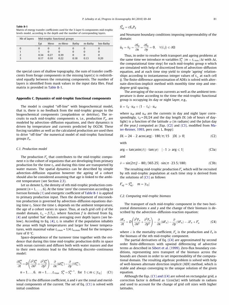
Table B-1Matrix of energy transfer coefficients used for the 3-layer 6-components mid-trophiclevels model, according to the depth and the number of corresponding layers.

Nb of layers Mid-trophic functional groups

Epi Meso m-Meso Bathy m-Bathy hm-Bathy

0 0 0 0 0 0 01 1 0 0 0 0 02 0.34 0.27 0.39 0 0 03 0.17 0.10 0.22 0.18 0.13 0.20


the special cases of shallow topography, the sum of transfer coeffi-cients from forage components in the missing layer(s) is redistrib-uted equally between the remaining components. The number oflayers is identified from mask values in the input data files. Finalmatrix is provided in Table B-1.

Appendix C. Dynamics of mid-trophic functional components

The model is coupled ‘‘off-line” with biogeochemical model,that is, there is no feedback from the mid-trophic groups to thebiogeochemical components (zooplankton or detritus). The re-cruits to each mid-trophic components n, i.e., production F 0n, aremodeled by advection–diffusion equations, and their dynamics isdriven by temperature and currents predicted by OGCM. Theseforcing variables as well as the calculated production are used thento drive ‘‘off-line” the numerical model of mid-trophic functionalgroups Fn.

C.1. Production model

The production F 0n that contributes to the mid-trophic compo-nent n is the cohort of organisms that are developing from primaryproduction for the time tr, and during this time are transported bywater masses. The spatial dynamics can be described by simpleadvection–diffusion equation however the ageing of a cohortshould also be considered assuming that age is linked to the ambi-ent temperature (see Section 2.3).

Let us denote Sn the density of nth mid-trophic production com-ponent (n = 1, . . . , 6). At the time ‘zero’ the conversion according toIverson formula (1) and energetic coefficient of Table B-1 is appliedto primary production input. Then the development of micronek-ton production is governed by advection–diffusion equations dur-ing time tr. Since the time tr depends on the ambient temperature,the age of a cohort varies in space. Thus, at each grid cell ij of themodel domain, trij

¼ f ðT ijÞ, where function f is derived from Eq.(4) and symbol ‘hat’ denotes averaging over depth layers (see be-low). According to Eq. (4), tr is smaller if the population inhabitsthe areas with high temperatures and larger for lower tempera-tures, with maximal value tr,max = 1/4 tm,max fixed for the tempera-ture of 0 �C.

Space-dependence of the turnover time together with the evi-dence that during this time mid-trophic production drifts in spacewith ocean currents and diffuses both with water masses and dueto their own motions lead to the following discrete–continuousmodel:

@Smn

@t¼D

@2Smn

@x2 þ@2Sm

n

@y2

!� @

@xðuSm

n Þ�@

@yðmSm

n Þ;

n¼1; . . . ;6; m¼1; . . . ;tr max Smn ¼ Sm�1

n ; for 16m6 btrijc ðC1Þ

where D is the diffusion coefficient, u and v are the zonal and merid-ional components of the current. The set of Eq. (C1) is solved withinitial condition

S0nij ¼ cEnPij

and Neumann boundary conditions imposing impermeability of thedomain:

uij ¼ vij ¼@Sij

@x¼ @Sij

@y¼ 0; 8ði; jÞ 2 @X

Thus, in order to resolve both transport and ageing problems atthe same time we introduce m variables Sm

n ðm ¼ tr max=Dt with Dt,the computational time step) for each mid-trophic group n whichare simulated with help of discretized form of advection–diffusionequation, and at each time step yield to simple ‘ageing’ relation-ships according to instantaneous integer values of trij

at each cellij. The finite-difference approximation of ADEs is solved with alter-nate-direction-implicit method with monthly time step and one-degree grid spacing.

The averaging of the ocean currents as well as the ambient tem-perature is done according to the time the mid-trophic functionalgroup is occupying its day or night layer, e.g.,

u ¼ sd � udl þ ð1� sdÞ � unl

where udl and unl are the currents in day and night layer corre-spondingly, sd = DL/24 and the day length DL (nb of hours of day-light) is a function of the latitude u (in radians) and the Julian dayof the year J computed as (Eqs. (C2) and (C3), modified from Ma-ier-Reimer, 1993, pers com. L. Bopp):

DL ¼ 24� 2 acosðargÞ � 180=p=15 ½DL P 0� ðC2Þ

with

arg ¼ tanðasinðdÞÞ � tanðuÞ ½�1 P arg 6 1� ðC3aÞ

and

d ¼ sin½2pðJ � 80Þ=365:25� � sinðp � 23:5=180Þ ðC3bÞ

The resulting mid-trophic production F 0n which will be recruitedby nth mid-trophic population at each time step is derived fromthe solutions of (C1) as follows

F 0nij ¼ Smnij; m ¼ ½trij�

C.2. Computing mid-trophic biomass

The transport of each mid-trophic component in the two hori-zontal dimensions x and y and the change of their biomass is de-scribed by the advection–diffusion-reaction equation:

@Fn

@t¼ D

@2Fn

@x2 þ@2Fn

@y2

!� @

@xðuFnÞ �

@

@yðvFnÞ � kFn þ F 0n ðC4Þ

where k is the mortality coefficient, F 0n is the production and Fn isthe biomass of the nth mid-trophic component.

The partial derivatives of Eq. (C4) are approximated by secondorder finite-differences with upwind differencing of advectiveterms as described in Sibert et al. (1999). Zero-flux boundary con-ditions, representing zero transport of the biomass across thebounds are chosen in order to set impermeability of the computa-tional domain. The resulting algebraic problem is solved with helpof well-known alternate direction implicit (ADI) method, which isstable and always converging to the unique solution of the givenequation.

Although the Eqs. (C1) and (C4) are solved on rectangular grid, acorrection factor is defined as 1/cos(lat) with latitude in radiansand used to account for the change of grid cell sizes with higherlatitudes.


Appendix D. Time of development at maturity and ambient temperature

Species
Taxa AmbientT(�C)
Age atmaturity (d)

Reference

Illex illecebrosus
Cephalopod 12.6 365 Wood and O’Dor (2000) Loligo vulgaris Cephalopod 14.0 245 Wood and O’Dor (2000) Loligo forbesi Cephalopod 14.0 365 Wood and O’Dor (2000) Loligo opalescens Cephalopod 16.0 184 Wood and O’Dor (2000) Ommastrephes bartramii Cephalopod 23 310 Ichii et al. (2004) Euprymna scolopes Cephalopod 23.0 80 Wood and O’Dor (2000) Idiosepius pygmaeus Cephalopod 25.2 50 Wood and O’Dor (2000) Sepioteuthis lessoniana Cephalopod 26.2 150 Forsythe et al. (2001) and Jackson and
Moltschaniwskyj (2002)
Sepioteuthis lessoniana Cephalopod 27 110 Forsythe et al. (2001) Tropical squids (Loliolus noctiluca, Loligo chinensis, Idiodepius
pygmaeus)
Cephalopod 28 120 Jackson and Choat (1992)
Sepiella inermis
Cephalopod 30.0 90 Wood and O’Dor (2000) Sepioteuthis lessoniana Cephalopod 30.0 90 Wood and O’Dor (2000) Sepioteuthis lessoniana Cephalopod 20.6 192 Forsythe et al. (2001) Pandalus borealis Crustacean 0 2009 Hansen and Aschan (2000) Pandalus borealis Crustacean 0 2191 Hansen and Aschan (2000) Pandalus borealis Crustacean 1 2557 Hansen and Aschan (2000) Pandalus borealis Crustacean 1.4 2191 Hansen and Aschan (2000) Pandalus borealis Crustacean 1.7 2009 Hansen and Aschan (2000) Pandalus borealis Crustacean 2.5 2557 Hansen and Aschan (2000) Pandalus borealis Crustacean 4 1826 Hansen and Aschan (2000) Pandalus borealis Crustacean 4.5 1095 Hansen and Aschan (2000) Nycthiphanes simplex Crustacean 24 60 Siegel (2000) Euphausia superba Crustacean 4 1095 Siegel (2000) Euphausia eximia Crustacean 18 210 Siegel (2000) Euphausia pacifica Crustacean 12 365 Siegel (2000) Metherytrops microphtalma Crustacean 2 912.5 Ikeda (1992) Thysanopoda tricuspidata, T. monocantha, T. aequalis,
Nematoscelis tenella, Euphausia diomedae
Crustacean 17 300 Roger (1971)
Mallotus villosus
Fish 4 1095 Carscadden et al. (1997) Leuroglossus schmidti Fish 5 730 Abookire et al. (2002) Stenobrachius leucopsarus Fish 5 1460 Abookire et al. (2002) Clupea harrengus Fish 8 1095 Reid et al. (1999) Clupea harrengus Fish 5 1278 Alheit and Hagen (1997) and Corten
(1999)
Engraulis ringens Fish 14 450 Schwartzlose et al. (1999) Engraulis japonicus Fish 16 300 Takahashi and Watanabe (2004) Engraulis mordax Fish 15 365 Schwartzlose et al. (1999) Engraulis capensis Fish 13 360 Schwartzlose et al. (1999) Engraulis encrasicolus Fish 10 400 Samsun et al. (2004) Engraulis encrasicolus Fish 13 365 Allain (2005) Sardinops melanostictus Fish 12 700 Hunter and Wada (1993) Sardinops sagax Fish 14 730 Schwartzlose et al. (1999) Encrasicholina punctifer Fish 30 120 Dalzell (1993) Vinciguerria Nimbarria Fish 28 120 Stéquert et al. (2003) Scomber japonicus Fish 12 730 Prager and MacCall (1988) Clupea pallasi Fish 7 1095 Hunter and Wada (1993)
References

Abookire, A.A., Piatt, J.F., Speckman, S.G., 2002. A nearsurface, daytime occurrence oftwo mesopelagic fish species (Stenobrachius leucopsarus and Leuroglossusschmidti) in a glacial fjord. Fishery Bulletin 100, 376–380.

Alheit, J., Hagen, E., 1997. Long-term climate forcing of European herring andsardine populations. Fisheries Oceanography 6 (2), 130–139.

Allain, G. (2005). Modélisation biophysique pour la prévision du recrutement.Couplage stochastique d’un modèle individu-centré de croissance larvaire avecun modèle hydrodynamique 3D pour développer un indice de recrutement del’anchois dans le golfe de Gascogne. Thèse de doctorat. Ecole NationaleSupérieure Agronomique de Rennes. France. 183 pp.

Allen, K.R., 1971. Relation between production and biomass. Journal of the FisheriesResearch Board of Canada 28, 1573–1581.

Belgrano, A., Allen, A.P., Enquist, B.J., Gillooly, J.F., 2002. Allometric scaling ofmaximum population density: a common rule for marine phytoplankton andterrestrial plants. Ecology Letters 5, 611–613.

Blackburn, M., 1968. Micronekton of the eastern tropical Pacific Ocean: familycomposition, distribution, abundance, and relations to tuna. Fishery Bulletin US67, 71–115.

Blackburn, M., Laurs, M.R., 1972. Distribution of Forage of skipjack Tuna (Euthynnuspelamis) in the Eastern Tropical Pacific. NOAA No. SSRF-649.

Boudreau, P.R., Dickie, L.M., 1992. Biomass spectra of aquatic ecosystems in relationto fisheries yield. Canadian Journal of Fisheries and Aquatic Sciences 46, 614–623.

Brown, J.H., Gilooly, J.F., Allen, A.P., Savage, V.M., West, G., 2004. Toward a metabolictheory of ecology. Ecology 85, 1771–1789.

Butterworth, D.S., Plaganyi, E.E., 2004. A brief introduction to some approaches tomultispecies/ecosystem modeling in the context of their possible application inthe management of South African fisheries. African Journal of Marine Science26, 53–61.

Carscadden, J., Nakashima, B.S., Frank, K.T., 1997. Effects of fish length andtemperature on the timing of peak spawning in capelin (Mallotus villosus).Canadian Journal of Fisheries and Aquatic Sciences 54, 781–787.


Chai, F., Dugdale, R.C., Peng, T.-H., Wilkerson, F.P., Barber, R.T., 2002. One-dimensional ecosystem model of the equatorial Pacific upwelling system, partI: model development and silicon and nitrogen cycle. Deep Sea Research II 49,2713–2745.

Chen, D., Rothstein, L.M., Busalacchi, A.J., 1994. A hybrid vertical mixing scheme andits application to tropical ocean models. Journal of Physical Oceanography 24,2156–2179.

Christensen, V., Pauly, D., 1992. Ecopath II – a software for balancing steady-stateecosystem models and calculating network characteristics. EcologicalModelling 61, 169–185.

Christian, J., Verschell, M., Murtugudde, R., Busalacchi, A., McClain, C., 2002.Biogeochemical modeling of the tropical Pacific Ocean I: Seasonal andinterannual variability. Deep Sea Research II 49, 509–543.

Christian, J.R., Murtugudde, R., 2003. Tropical Atlantic variability in a coupledphysical–biogeochemical ocean model. Deep Sea Research II 50 (22–26), 2947–2969.

Coale, K.H., Johnson, K.S., Fitzwater 16 co-authors, S.E., 1996. A massivephytoplankton bloom induced by an ecosystem-scale iron fertilizationexperiment in the equatorial Pacific Ocean. Nature 383, 495–501.

Corten, A., 1999. The reappearance of spawning Atlantic herring (Clupea harengus)on Aberdean Bank (North Sea) in 1983 and its relationship to environmentalconditions. Canadian Journal of Fisheries and Aquatic Sciences 56, 2051–2061.

Cushing, D.H., 1975. Marine Ecology and Fisheries. Cambridge Univ. Press,Cambridge, England. 278 p..

Dalzell, P.J., 1993. Small pelagic fishes. In: Wright, A., Hill, L. (Eds.), NearshoreMarine Resources of the South Pacific. IPS, Suva, FFA, Honiara, ICOD, Canada, pp.97–133.

Dickie, L.M., 1976. Predation, yield and ecological efficiency in aquatic food chains.Journal of the Fisheries Research Board of Canada 33, 313–316.

Dugdale, R.C., Barber, F., Chai, F., Peng, T.H., Wilkerson, F.P., 2002. One dimensionalecosystem model of the equatorial Pacific upwelling system, part II: sensitivityanalysis and comparison with JGOFS EqPac data. Deep Sea Research II 49 (13–14):2746–2762.

Elton, C., 1927. Animal Ecology. Macmillan, New York, NY. 207 pp.Enquist, B.J., Brown, J.H., West, G.B., 1998. Allometric scaling of plant energetics and

population density. Nature 395, 163–165.Fenchel, T., 1974. Intrinsic rate of natural increase: the relationship with body size.

Oecologia 14, 317–326.Forsythe, J.W., Walsh, L.S., Turk, P.E., Lee, P.G., 2001. Impact of temperature on

juvenile growth and age at first egg-laying of the Pacific reef squid Sepioteuthislessoniana reared in captivity. Marine Biology 138, 103–112.

Froese, R., Binohlan, C., 2000. Empirical relationships to estimate asymptotic length,length at first maturity and length at maximum yield per recruit in fishes, witha simple method to evaluate length frequency data. Journal of Fish Biology 56,758–773.

Gaspar, P., Grégoris, Y., Lefevre, J.M., 1990. A simple eddy-kinetic energy model forsimulations of the oceanic vertical mixing: tests at station Papa and long-termupper Ocean study site. Journal of Geophysical Research-Oceans 95, 16179–16193.

Gillooly, J.F., Charnov, E.L., West, G.B., Savage, V.M., Brown, J.H., 2002. Effects of sizeand temperature on developmental time. Nature 417, 70–73.

Grandperrin, R., 1975. Structures trophiques aboutissant aux thons de longueslignes dans le Pacifique sud-ouest tropical. Thèse de Doctorat, Université deMarseille.

Hansen, H.O., Aschan, M., 2000. Growth, size and age-at-maturity of shrimp,Pandalus borealis, at Svalbard, related to environmental parameters. Journal ofNorthwestern Atlantic Fisheries Science 27, 83–91.

Hidaka, K., Kawaguchi, K., Tanabe, T., Takahashi, M., Kubodera, T., 2003. Biomass andtaxonomic composition of micronekton in the western tropical–subtropicalPacific. Fisheries Oceanography 12 (2), 112–125.

Hjort, J., 1914. Fluctuations in the great fisheries of northern Europe. Rapp. P.-V.Reun. Cons. Int. Explor. Mer 20,1–227.

Hunter, J.R., Wada, T. (Eds.), 1993. PICES Scientific Report No. 1. Part 1. CoastalPelagic Fishes. Publish. North Pacific Marine Science Organisation (PICES), 131pp.

Huntley, M.E., Zhou, M., 2004. Influence of animals on turbulence in the sea. MarineEcology Progress Series 273, 65–79.

Ichii, T., Mahapatra, K., Sakai, M., Inagake, D., Yoshihiro, O., 2004. Differing body sizebetween the autumn and the winter–spring cohorts of neon flying squid(Ommastrephes bartramii) related to the oceanographic regime in the NorthPacific: a hypothesis. Fisheries Oceanography 13 (5), 295–309.

Ikeda, T., 1992. Growth and life history of the mesopelagic mysid Meterythropsmicrophthalma in the southern Japan Sea. Journal of Plankton Research 14 (12),1767–1779.

Iverson, R.L., 1990. Control of marine fish production. Limnology Oceanography 35,1593–1604.

Jackson, G.D., Choat, J.H., 1992. Growth in tropical cephalopods: an analysis basedon statolith microstructure. Canadian Journal of Fishery and Aquatic Sciences49, 218–228.

Jackson, G.D., Moltschaniwskyj, N.A., 2002. Spatial and temporal variation in growthrates and maturity in the Indo-Pacific squid Sepioteuthis lessoniana(Cephalopoda: Loliginidae). Marine Biology 140, 747–754.

Jennings, S., Warr, K.J., Mackinson, S., 2002. Use of size-based production and stableisotope analyses to predict trophic transfer efficiencies and predator–prey bodymass ratios in food webs. Marine Ecology Progress Series 240, 11–20.

Kerr, S.R., 1974. Theory of size distribution in ecological communities. JournalFisheries Research Board of Canada 31, 1859–1862.

King, J.E., Iversen, R.T.B., 1962. Midwater trawling for forage organisms in thecentral Pacific, 1951–1956. Fishery Bulletin US 210, 271–321.

Kleiber, M., 1932. Body size and metabolism. Hilgardia 6, 315–353.Kobayashi, H.A., 1974. Growth cycle and related vertical distribution of the

Thecosomatous Pteropod Spiratella (‘‘Limacina”) helicina in the central ArcticOcean. Marine Biology 26, 295–301.

Kooijman, S.A.L.M., 1986. Energy budgets can explain body size relations. Journal ofTheoretical Biology 121, 269–282.

Kunze, E., Dower, J.F., Beveridge, I., Dewey, R., Bartlett, K.P., 2006. Observations ofbiologically generated turbulence in a coastal inlet. Science 313 (5794), 1768–1770.

Legand, M., Bourret, P., Fourmanoir, R., Grandperrin, R., Gueredrat, J.A., Michel, A.,Rancurel, P., Repelin, R., Roger, C., 1972. Relations trophiques et distributionsverticales en milieu pélagique dans l’Océan Pacifique intertropical. CahierORSTOM. Série Océanographique 10 (4), 303–393.

Lehodey, P., Andre, J.-M., Bertignac, M., Hampton, J., Stoens, A., Menkes, C., Memery,L., Grima, N., 1998. Predicting skipjack tuna forage distributions in theequatorial Pacific using a coupled dynamical bio-geochemical model.Fisheries Oceanography 7 (3/4), 317–325.

Lehodey, P., Chai, F., Hampton, J., 2003. Modeling climate-related variability of tunapopulations from a coupled ocean-biogeochemical-populations dynamicsmodel. Fisheries Oceanography 12 (4), 483–494.

Lehodey, P., 2001. The pelagic ecosystem of the tropical Pacific Ocean: dynamicspatial modeling and biological consequences of ENSO. Progress inOceanography 49, 439–468.

Lehodey, P., 2004a. Climate and fisheries: an insight from the Pacific Ocean. In:Stenseth, N.C., Ottersen, G., Hurrel, J., Belgrano, A. (Eds.), Ecological Effects ofClimate Variations in the North Atlantic. Oxford University press, pp. 137–146.

Lehodey, P., 2004b. A spatial ecosystem and populations dynamics model(SEAPODYM) for tuna and associated oceanic top-predator species: part I –lower and intermediate trophic components. In: 17th Meeting of the StandingCommittee on Tuna and Billfish, Majuro, Republic of Marshall Islands, 9–18Aug. 2004, Oceanic Fisheries Programme, Secretariat of the Pacific Community,Noumea, New Caledonia, SCTB Working Paper: ECO-1. 26 pp.

Lehodey, P., Senina, I., Murtugudde, R., 2008. A spatial ecosystem and populationsdynamics model (SEAPODYM) – modeling of tuna and tuna-like populations.Progress in Oceanography 78, 304–318.

Lindeman, R.L., 1942. The trophic-dynamic aspect of ecology. Ecology 23, 399–418.McClatchie, S., Dunford, A., 2003. First estimate of the biomass of vertically

migrating mesopelagic fish off New Zealand. Deep Sea Research I 50, 1263–1281.

Maier-Reimer, E., 1993. Geochemical cycles in an ocean general circulation model.Preindustrial tracer distributions. Global Biogeochemical Cycles 7, 645–677.

Martin, J.H., Coale, K.H., Johnson, K.S., Fitzwater 40 authors, S.E., 1994. Testing theiron hypothesis in ecosystem of the equatorial Pacific Ocean. Nature 371, 123–129.

Martin, J.H., 1990. Glacial–interglacial CO2 change: the iron hypothesis.Paleoceanography 5 (1), 1–13.

Maury, O., Faugeras, B., Shina, Y.-J., Poggialeb, J.-C., Ben Aria, T., Marsac, F., 2007.Modeling environmental effects on the size-structured energy flow throughmarine ecosystems. Part 1: the model. Progress in Oceanography 74, 479–499.

Murtugudde, R., Beauchamp, J., McClain, C., Lewis, M., Busalacchi, A.J., 2002. Effectsof penetrative radiation on the upper tropical ocean circulation. Journal ofClimate 15, 470–486.

Murtugudde, R., Seager, R., Busalacchi, A., 1996. Simulation of the tropical oceanswith an ocean GCM coupled to an atmospheric mixed layer model. Journal ofClimate 9, 1795–1815.

Murtugudde, R.G., Wang, L., Hackert, E., Beauchamp, J., Christian, J.R., Busalacchi,A.J., 2004. Remote sensing of the Indo-Pacific region: Ocean color, sea level,winds, and SSTs. International Journal of Remote Sensing 25 (7–8), 1423–1435.

Palomares, M.L., Muck, P., Mendo, J., Chuman, E., Gomez, O., Pauly, D., 1987. Growthof the Peruvian anchoveta (Engraulis ringens), 1953 to 1982. In: Pauly, D.,Tsukayama, I. (Eds.), The Peruvian Anchoveta and its Upwelling Ecosystems:Three Decades of Change, vol. 15. pp 117-141.

Parrish, R.H., Bakun, A., Husby, D.M., Nelson, C.S., 1983. Comparative climatology ofselected environmental processes in relation to eastern boundary currentpelagic fish reproduction. FAO Fisheries Report 293 (3), 731–777 (Proc. TheExpert Consultation to Examine Changes in Abundance and SpeciesComposition of Neritic Fish Resources, San JoseÂ, Costa Rica).

Platt, T., Denman, K.L., 1978. The structure of the pelagic marine ecosystems. Rapp.P.-V. Réunion Du Conseil International pour l’Exploration de la Mer 173, 60–65.

Platt, T., 1985. Structure of the marine ecosystem: its allometric basis. CanadianBulletin of Fisheries and Aquatic Sciences 213, 55–64.

Plimpton, P.E., Freitag, H.P., McPhaden, M.J., 2004. Processing of Subsurface ADCPData in the Equatorial Pacific. /NOAA Tech. Mem./OAR PMEL-125. 41 pp.

Prager, M.H., MacCall, A.D., 1988. Revised estimates of historical spawning biomassof the Pacific mackerel, Scomber japonicus. CalCOFI Reports 29, 81–90.

Reid, R.N., Cargnelli, L.M., Griesbach, S.J., Packer, D.B., Johnson, D.L., Zetlin, C.A.,Morse, W.W., Berrien, P.L., 1999. Essential Fish Habitat Source Document:Atlantic Herring, Clupea harengus, Life History and Habitat Characteristics. USNOAA Technical Memorandum NMFS NE-126. 56 pp.

Repelin, R., 1978. Les amphipodes pélagiques du Pacifique occidental et central:biologie, écologie et relations trophiques avec la faune ichthyologique. Travauxet Documents de l’ORSTOM 86. 381 pp.


Ricker, W.E., 1975. Computation and interpretation of biological statistics of fishpopulations. Bulletin of Fisheries Research Board Canada. 191. 382 pp.

Roger, C., 1971. Les euphausiacés du Pacifique équatorial et sud tropical. Thèse deDoctorat, Université de Provence – ORSTOM.

Samsun, O., Samsun, N., Karamollaoglu, A.C., 2004. Age, growth, mortality rates ofthe European anchovy (Engraulis encrasicolus, L. 1758) Off the Turkish Black Seacoast. Turkish Journal of Veterinary and Animal Science 28, 901–910.

Savage, V.M., Gilllooly, J.F., Brown, J.H., West, G.B., Charnov, E.L., 2004. Effect of bodysize and temperature on population growth. The American Naturalist 163 (3),429–441.

Schwartzlose, R.A., Alheit, J., Bakun, A., Baumgartner 17 authors, T.R., 1999.Worldwide large-scale fluctuations of sardine and anchovy populations. SouthAfrican Journal of Marine Sciences 21, 89–347.

Senina, I., Sibert, J., Lehodey, P., 2008. Parameter estimation for basin-scaleecosystem-linked population models of large pelagic predators: application toskipjack tuna. Progress in Oceanography 78, 319–335.

Sheldon, R.W., Prakash, A., Sutcliffe Jr., W.H., 1972. The size distribution of particlesin the Ocean. Limnology Oceanography 17, 327–340.

Sibert, J.R., Hampton, J., Fournier, D.A., Brills, P.J., 1999. An advection–diffusion-reaction model for the estimation of fish movement parameters from taggingdata, with application to skipjack tuna (Katsuwonus pelamis). Canadian Journalof Fisheries and Aquatic Sciences 56, 925–938.

Siegel, V., 2000. Krill (Euphausiacea) life history and aspects of population dynamics.Canadian Journal of Fishery and Aquatic Sciences 57 (Suppl. 3), 130–150.

Stéquert, B., Ménard, F., Marchal, E., 2003. Reproductive biology of Vinciguerrianimbaria in the equatorial waters of the eastern Atlantic Ocean. Journal of FishBiology 62, 1116–1136.

Takahashi, M., Watanabe, Y., 2004. Growth rate-dependent recruitment of Japaneseanchovy Engraulis japonicus in the Kuroshio–Oyashio transitional waters.Marine Ecology Progress Series 266, 227–238.

Van der Meer, J., 2006. Metabolic theories in ecology. Trends in ecology andevolution 21 (3), 136–140.

Vinogradov, M.E., 1981. Ecosystems of equatorial upwellings. In: Longhurst, A.R.(Ed.), Analysis of Marine Ecosystems. Academic Press, pp. 69–93.

Wang, X., Christian, J.R., Murtugudde, R., Busalacchi, A.J., 2005. Ecosystem dynamicsand export production in the central and eastern equatorial Pacific: a modelingstudy of impact of ENSO. Geophysical Research Letter 32, L2608.

Wang, X., Christian, J.R., Murtugudde, R., Busalacchi, A.J., 2006a. Spatial andtemporal variability of the surface water pCO2 and air–sea CO2 flux in theequatorial Pacific during 1980–2003: a basin-scale carbon cycle model.Geophysical Research Letter 111, C07S04.

Wang, X., Christian, J.R., Murtugudde, R., Busalacchi, A.J., 2006b. Spatial andtemporal variability in new production in the equatorial Pacific during 1980–2003: physical and biogeochemical controls. Deep Sea Research II 53, 677–697.

West, G.B., Brown, J.H., Enquist, B.J., 1997. A general model for the origin ofallometric scaling laws in biology. Science 276, 122–126.

West, G.B., Brown, J.H., Enquist, B.J., 2001. A general model for ontogenic growth.Nature 413, 628–631.

Wiggert, J.D., Murtugudde, R., Christian, J.R., 2006. Annual ecosystem variability inthe tropical Indian Ocean: results of a coupled bio-physical ocean generalcirculation model. Deep Sea Research 53, 644–676.

Wood, J.B., O’Dor, R.K., 2000. Do larger cephalopods live longer? Effects oftemperature and phylogeny on interspecific comparisons of age and size atmaturity. Marine Biology 136, 91–99.

Bridging the gap from ocean models to population...

Documents

Transcript of Bridging the gap from ocean models to population...