HAL Id: hal-02515637https://hal-normandie-univ.archives-ouvertes.fr/hal-02515637

Preprint submitted on 23 Mar 2020

HAL is a multi-disciplinary open accessarchive for the deposit and dissemination of sci-entific research documents, whether they are pub-lished or not. The documents may come fromteaching and research institutions in France orabroad, or from public or private research centers.

L’archive ouverte pluridisciplinaire HAL, estdestinée au dépôt et à la diffusion de documentsscientifiques de niveau recherche, publiés ou non,émanant des établissements d’enseignement et derecherche français ou étrangers, des laboratoirespublics ou privés.

Bridging the Gap Between Spectral and SpatialDomains in Graph Neural Networks

Muhammet Balcilar, Guillaume Renton, Pierre Héroux, Benoît Gaüzère,Sébastien Adam, Paul Honeine

To cite this version:Muhammet Balcilar, Guillaume Renton, Pierre Héroux, Benoît Gaüzère, Sébastien Adam, et al..Bridging the Gap Between Spectral and Spatial Domains in Graph Neural Networks. 2020. �hal-02515637�

PREPRINT 1

Bridging the Gap Between Spectral and SpatialDomains in Graph Neural Networks

Muhammet Balcilar, Guillaume Renton, Pierre Heroux, Benoit Gauzere, Sebastien Adam,and Paul Honeine

Abstract—This paper aims at revisiting Graph Convolutional Neural Networks by bridging the gap between spectral and spatial designof graph convolutions. We theoretically demonstrate some equivalence of the graph convolution process regardless it is designed in thespatial or the spectral domain. The obtained general framework allows to lead a spectral analysis of the most popular ConvGNNs,explaining their performance and showing their limits. Moreover, the proposed framework is used to design new convolutions inspectral domain with a custom frequency profile while applying them in the spatial domain. We also propose a generalization of thedepthwise separable convolution framework for graph convolutional networks, what allows to decrease the total number of trainableparameters by keeping the capacity of the model. To the best of our knowledge, such a framework has never been used in the GNNsliterature. Our proposals are evaluated on both transductive and inductive graph learning problems. Obtained results show therelevance of the proposed method and provide one of the first experimental evidence of transferability of spectral filter coefficients fromone graph to another.

Index Terms—Graph Convolutional Neural Networks, Spectral Graph Filter.

F

1 INTRODUCTION

O VER the past decade, Deep Learning, and more specif-ically Convolutional Neural Networks (CNNs) and

Recurrent Neural Networks (RNNs), had a strong impactin various applications of machine learning, such as imagerecognition [1] and speech analysis [2]. These successeshave mostly been achieved on sequences or images, i.e. ondata defined on grid structures which benefit from linearalgebra operations in Euclidean spaces. However, there aremany domains where data (e.g. social networks, molecules,knowledge graph) cannot be trivially encoded into an Eu-clidean domain, but can be naturally represented as graphs.

This explains the recent challenge tackled by the machinelearning community which consists in transposing the deeplearning paradigm into the world of graphs. The objectiveis to revisit Neural Networks to operate on graph data,in order to benefit from the representation learning ability.In this context, many Graph Neural Networks (GNNs)have been recently proposed in the literature of geometriclearning [3], [4], [5], [6]. GNNs are Neural Networks thatrely on the computation of hidden representations of nodesusing information carried by the whole graph. In contrastto conventional Neural Network, where the architecture ofthe network is related to the known and invariant topologyof the data (e.g. a 2-D grid for images), the node features ofGNNs are propagated according to the graph topology.

Among GNNs, Convolutional GNNs (ConvGNNs) aimto mimic the simple and efficient solution provided by CNNto extract features through a weight-sharing strategy alongthe presented data. In images, a convolution relies on thecomputation of a weighted sum of neighbor’s features andweight-sharing is possible thanks to the neighbor relative

• All the authors are with Normandie Univ, UNIROUEN, UNIHAVRE,INSA Rouen, LITIS, 76000 Rouen, France.E-mail: muhammetbalcilar@gmail.com

positions. With graph-structured data, designing such aconvolution process is not straightforward. First, there is avariable and unbounded number of neighbors, avoiding theuse of a fixed sized window to compute the convolution.Second, no order exists on node neighborhood. As a conse-quence, one may first redefine the convolution operator todesign a ConvGNN.

As in images, a graph convolution process correspondsto the multiplication of a convolution kernel with the cor-responding node feature vectors, followed by a sum or amean rule. In the literature, there are some instances oftrainable and non-trainable convolution kernels for graphs.Regardless if the convolution kernels are trainable or not,and according to the convolution theorem, two strategieshave been investigated to design filter kernels, based eitheron the spectral or the spatial domains.

Spectral-based convolution filters are defined from agraph signal processing point of view. In a nutshell, a basis isdefined by the eigendecomposition of the graph Laplacianmatrix. This allows to define the graph Fourier transform,and thus the graph filtering operators. The original formof the spectral graph convolution (non-parametric) can bedefined by a function of frequency (eigenvalues). Therefore,this method can theoretically extract information on anyfrequency. However, despite the solid mathematical founda-tions borrowed from the signal processing literature, suchapproaches suffer from (i) a large computational burdeninduced by the forward/inverse graph Fourier transform,(ii) being spatially non-localized and (iii) the transferabilityproblem, i.e., filters designed using a given graph cannotbe applied on other graphs. To alleviate these issues, someapproaches based on parameterization using B-spline [7],Chebyshev polynomials [8] and Cayley polynomials [9]have been proposed. However, these approaches cannotuse custom designed frequency response convolution, but

PREPRINT 2

only the one determined by B-spline, Chebyshev or Cay-ley polynomials. That means these methods cannot extractinformation on some custom band.

The second strategy is the spatial-based convolution,which is an extension of the conventional Euclidean convo-lution (e.g. 2D convolution in CNN), by aggregating nodesneighborhood information. Such convolutions have beenvery attractive due to their less computational complexity,their localized property and their transferability. Spatial-designed graph convolutions have to be a function of somespatial properties of graphs, such as adjacency, Laplacian ordegree matrix combined with feature of connected nodes,and edge features. However, since they are designed in thespatial domain, their spectral behavior is not taken intoaccount. We will show in the following that most of theexisting spatial-designed convolutions are essentially low-pass filters. As a consequence, they do not have the ability toextract useful information on high frequency or some certainfrequency bands. Yet, considering high-frequency informa-tion may be intuitively useful for some real-world problemswhere information localized on particular nodes have astrong influence on graph’s property. For instance, molec-ular toxicity can be induced by some pharmacophores, i.e.,particular subparts of molecule, which can consist in onlyone atom. Using only low-pass filters on such moleculeswill diffuse this discriminant information within the wholegraph whereas a high-pass filter may help to highlight thisuseful difference.

ContributionsIn this paper, we bridge the gap between spectral and spatialdomains for ConvGNNs. Our first contribution consistsin demonstrating the equivalence of convolution processesregardless if they are designed in the spatial or the spec-tral domain. Taking advantage of this result, our secondcontribution is to provide a spectral analysis of existinggraph convolutions for four popular ConvGNNs, knownas GCN [10], ChebNet [8], CayleyNet [9] and Graph At-tention Networks (GAT) [11]. Using these results, our thirdcontribution is to design new convolutions in the spectraldomain with a custom frequency profile that provides abetter convolution process. In this context, we also proposea spectral-designed multi-convolution method under thedepthwise separable convolution framework. To the best ofour knowledge, such a framework has never been used inthe GNNs literature. It allows to decrease the total numberof trainable parameters by keeping the variability capacityof the model at a maximum level.

Our proposal is assessed on both transductive and in-ductive learning problems [12]. In both settings, we showthe relevance of the proposed method on well-known publicbenchmark datasets. Especially, the success of the proposedmethod on inductive problems provides one of the firstexperimental evidence of transferability of spectral filtercoefficients from one graph to another.

The remainder of this paper is organized as follows. InSection 2, we introduce ConvGNNs and we review exist-ing approaches. Then, Section 3 describes the three maincontributions mentioned above. Section 4 presents a seriesof experiments and results which validate our propositions.Finally, Section 5 is dedicated to the conclusion.

2 CONVGNN: PROBLEM STATEMENT AND STATEOF THE ART

2.1 Graph Learning Problems

Let G be a set of graphs, where each graph G(k) has nknodes and an arbitrary number of edges. Node-to-nodeconnectivity in G(k) is given by the adjacency matrix A(k).For unweighted graphs, A(k) ∈ {0, 1}nk×nk , while forweighted graphs, A(k) ∈ Rnk×nk . In this paper, we considerundirected attributed graphs. Hence, A(k) is symmetric andfeatures are defined on nodes by X(k) ∈ Rnk×f0 , with f0the length of feature vectors.

In the literature, there are three different types of learn-ing problems on graphs. The first one is the single graphnode classification or regression problem. In this case, G isreduced to a single graph denoted G, with n nodes. Some ofthe nodes are labeled for training and the task is to predictthe labels of unlabeled nodes. For a classification problem,the output would be represented by Y ∈ {0, 1}n×nc , i.e., aone-hot class encoding of the nc possible classes for eachnode. For a node regression problem, the output wouldbe Y ∈ Rn. The second type of problems is multi-graphnode classification or regression problem. In such cases,the output is defined as a set of Y(k) ∈ {0, 1}nk×nc forclassification or Y(k) ∈ Rnk for regression. The last typeis the entire graph classification or regression problem, inwhich case the output must be Y(k) ∈ {0, 1}nc or Y(k) ∈ Rfor classification and regression problems, respectively.

Problems of the first type are transductive problems,while problems of the two last types are inductive since testdata are completely unknown during training.

2.2 Literature review

For reviewing ConvGNNs, we use the classical “spectral vs.spatial” dichotomy [13]. Beyond, we propose for this reviewa third category called Spectral-Rooted Spatial Convolutionswhich gathers recent and efficient methods that take theirfoundations in the spectral domain, but apply them in thespatial one, without computing the graph Fourier transform.

2.2.1 Spectral ConvGNNSpectral ConvGNNs rely on the spectral graph theory [14].In this framework, signal on graphs are filtered using eigen-decomposition of graph Laplacian [15]. A graph Laplacianis defined by L = D − A (or L = I − D−1/2AD−1/2 forthe normalized version), where A is the adjacency matrix,D ∈ Rnk×nk is the diagonal degree matrix with entriesDi,i =

∑j Aj,i and I is the identity matrix. Since the

Laplacian is positive semidefinite, it can be decomposedinto L = UΣUT where U is the eigenvectors matrix andΣ = diag(λ) where λ denotes the vector of the positiveeigenvalues. The graph Fourier transform of any unidimen-sional signal on graph is defined by xft = U>x and its in-verse is given by x = Uxft. By transposing the convolutiontheorem to graphs, the spectral filtering in the frequencydomain can be defined by

xfiltered = U diag(z(λ))U>x, (1)

where z(λ) is the desired filter function applied to theeigenvalues λ. As a consequence, a graph convolution layer

PREPRINT 3

in spectral domain can be written by a sum of filtered signalsfollowed by an activation function as in [7], namely

H(l+1)j = σ

(fl∑i=1

U diag(Fi,j,l)U>H

(l)i

), (2)

for all j ∈ {1, . . . , fl+1}. Here, σ is the activation functionsuch as RELU (REctified Linear Unit), H(l)

i is the i-th featurevector of the l-th layer, Fi,j,l ∈ Rn is the correspondingweight vector whose size is the number of eigenvectors (alson, the number of nodes). A spectral ConvGNN based on (2)seeks to tune the trainable parameters Fi,j,l, as proposedin [16] for the single-graph problem. A first drawback is thenecessity of Fourier and inverse Fourier transform by matrixmultiplication ofU andUT . Another drawback occurs whengeneralizing the approach to multi-graph learning prob-lems. Indeed, the k-th element of the vector Fi,j,l weightsthe contribution of the k-th eigenvector to the output. Thoseweights are not shareable between graphs of different sizes,which means a different length of Fi,j,l is needed. Moreover,even though the graphs have the same number of nodes,their eigenvalues will be different if their structures differ.As a consequence, a given weight Fi,j,l may correspond todifferent eigenvalues in different graphs.

To overcome these issues, a few spatially-localized filtershave been defined such as cubic B-spline parameterization[7] and polynomial parameterization [8]. With such ap-proaches, trainable parameters are defined by:

Fi,j,l = B[W

(l,1)i,j , . . . ,W

(l,S)i,j

]>, (3)

where B ∈ Rn×S is the initial designed matrix and W (l,s)

is the trainable matrix for the l-th layer’s s-th convolu-tion kernel, W (l,s)

i,j is the (i, j)-th entry of W (l,s) and S isthe desired number of convolution kernels. Each columnin B is designed as a function of eigenvalues, namelyBi,j = (zj(λi)). In the polynomial case, each column of B ispower of eigenvalues starting at 0-th and ending at (S− 1)-th power. In the cubic B-spline case, the B matrix encodesthe cubic B-spline coefficients [7]. A very recent ConvGNNnamed CayleyNet parameterizes trainable coefficients byFi,j,l = [gi,j,l(λ1, h), ..., gi,j,l(λn, h)]>, where h is a scaleparameter to be learned, λn is the n-th eigenvalue, and gis a spectral filter function defined as follows in [9]:

g(λ, h) = c0 + 2Re

(r∑

k=1

ck

(hλ− ihλ+ i

)k)(4)

where i2 = −1, Re(·) is the function returning the real part,c0 is a real trainable coefficient, and for k = 1, . . . , r, ck arethe complex trainable coefficients. The CayleyNet parame-terization takes also the form (3), as shown in Appendix B.

2.2.2 Spatial ConvGNNSpatial ConvGNNs can be generalized as propagation ofnode features to the neighborhood nodes followed by ac-tivation function, of the form

H(l+1) = σ(∑

s

C(s)H(l)W (l,s)), (5)

where H(l) ∈ Rn×fl is the l-th layer’s feature matrixwith n nodes and fl features, s indexes the convolution

Fig. 1. Schematic of the GCN layer defined in (5). The graph has 12nodes and 12 edges. Each node has a 2-length feature vector H(l)

1 andH

(l)2 represented by colors. The second layer has a 3-length feature

vector, denoted H(l+1)1 , H(l+1)

2 and H(l+1)3 . Two convolution kernels

C(1) and C(2) are used. This architecture has 12 trainable parameters,omitting biases.

kernels, C(s) is the convolution kernel that defines how thenode features are propagated to the neighborhood nodes,W (l,s) ∈ Rfl×fl+1 is the trainable weight matrix that mapsthe fl-dimensional features into fl+1 dimensions. Fig. 1provides a detailed schematic of graph convolution layer ona sample graph signal. The selection of convolution kernelsdefines the method in the literature. The vanilla versionuses a single convolution kernel with C = A + I . Such aspatial ConvGNN has an effect of low-pass filtering, since itapplies the same coefficients to all neighbors and to the nodeitself. High-pass filters can be obtained by differentiatingthe weight matrices used to compute neighbors and self-contributions [17]. In such a case, the convolution process isgiven by C(1) = A and C(2) = I .

Some solutions have been proposed to overcome thelimitations of using only low-pass and high-pass filters.If nodes have discrete labels (unless the node’s degreecan be used as discrete feature), weights can be sharedby the neighbors whose labels are the same [18]. Anothermethod consists in defining an ordering on nodes includedwithin the receptive field of convolution, and sharing thecoefficients according to this reordering [19]. The reorderingprocess is called canonical node reordering. A similar shar-ing approach, based on reordered neighbors, was presentedin [20]. The difference is that the reordering is computedaccording to the absolute correlation of features to the centernode. A different spatial-designed method proposed in [21]considers a diffusion process on the graph using randomwalks. This allows to induce variability on output signal byapplying random walks of different lengths to the differentfeatures.

All aforementioned spatial graph convolutions use fixed-design matrices C(s) and variability is induced by W (l,s)

in (5). Other methods use trainable convolution kernels inorder to make the convolutions more productive in termsof output signal frequency profiles, such as graph attentionnetworks [11], [22], MoNet [23] and SplineCNN [24]. Theattention mechanism tunes each element of the convolution

PREPRINT 4

kernel of the l-th layer C(l,s), which is defined as a functionof connected nodes features and some trainable parameter

C(l,s)i,j = f

(H

(l)i , H

(l)j ,W

(l,s)AT

), (6)

where H(l)i ∈ Rfl is the i-th node’s feature vector for

layer l, W (l,s)AT encodes the trainable parameter of the s-

th convolution kernel for layer l and f is some element-wise function to be selected. In this case, since convolutionkernels are learned through the W (l,s)

AT of (6), the trainableparameters W (l,s) of (5) can be defined as the identity ma-trix, or other trainable parameters that may be shared withW

(l,s)AT . The most influential attention mechanism applied on

graph data, called GAT [11], uses multi-attention weights(denoted as multi-support convolution kernels), with

f(H

(l)i , H

(l)j ,W

(l,s)AT

)=softmaxj

(σ(a[WH

(l)i ||WH

(l)j ])

),

(7)where two linear transformations are considered by ele-ments of general trainable parameter set W (l,s)

AT = {a,W},with a being a weight vector. The operator || is the con-catenation operator, σ corresponds to the LeakyReLU func-tion [25] and softmaxj is the normalized exponential func-tion that uses all neighbors of i-th node to normalize edge ofi-th to j-th node. In convolution layer’s output calculation(5), GAT proposes to use the same parameters W. The mainlimitation of this method is the use of a very small context,limited to the features of the pair of nodes, to determinethe intensity of the attention. Dual-Primal Graph CNN(DPGCNN) [26] extends this approach by defining attentionusing new features computed from the neighborhood ofeach node of the pair, hence using a larger context.

Since the methods mentioned above are defined in thespatial domain, they do not provide any analysis of theirfrequency spectrum of filters. Moreover, their frequencyresponses will be different for different graphs. Besides, theyneed more multi-support (attention or sub-layer weights) toproduce high variability output, which drastically increasesthe number of trainable parameters of the model.

2.2.3 Spectral-rooted Spatial ConvolutionsAs said before, some methods have recently been proposedto get rid of the computation burden of graph Fourier andinverse graph Fourier transforms, while still taking theirfoundations in the spectral domain. These solutions rely onthe approximation of a spectral graph convolution proposedin [27], based on the Chebyshev polynomial expansionof the scaled graph Laplacian. Accordingly, the first twoChebyshev kernels are C(1) = I and C(2) = 2L/λmax − Iand the remaining kernels are defined by

C(k) = 2C(2)C(k−1) − C(k−2). (8)

Researchers have shown that any desired filter can be writ-ten as a linear combination of these kernels [27]. ChebNet isthe first method that used these kernels in ConvGNN [8].

One major extension and simplification of the Cheby-shev polynomial expansion method is Graph ConvolutionNetwork (GCN) [10]. GCN uses the subtraction of thesecond Chebyshev kernels from the first one under theassumption of λmax = 2 and L is the normalized graph

Laplacian. However, instead of using this subtracted kernel,they used re-normalization trick and defined the final singlekernel by:

C = D−1/2AD−1/2, (9)

with Di,i =∑j Ai,j and A = (A + I) the adjacency ma-

trix with added self-connections. This approach influencedmany other contributions. The method described in [28]directly uses this convolution but changes the network ar-chitecture by adding a fully connected layer as the last layer.The MixHop algorithm [29] uses the 2nd or 3rd powers ofthe same convolution.

The methods described in this section are quite differentfrom pure spatial and pure spectral convolutions. Theyare not designed by using eigenvalues, but are implicitlydesigned as a function of structural information (adjacency,Laplacian) and perform convolution in spatial domain ashow all spatial convolutions do. However, their frequencyprofiles are stable for different arbitrary graphs as howspectral convolutions do. This aspect will be theoreticallyand experimentally illustrated in the following sections.

3 BRIDGING SPATIAL AND SPECTRAL CONVGNNThis section presents the main theoretical contributions ofthis paper. First, we provide a theoretical analysis demon-strating that parameterized spectral ConvGNNs can be im-plemented as spatial ConvGNNs when they use a fixedfrequency profile matrix B. Then, using this result, somestate-of-the-art GNNs described in the previous section areanalyzed from a spectral point of view. This analysis providea better understanding on these convolutions and revealtheir problematic sides. Finally, we propose a new methodthat fully exploits spectral graph convolution capabilities,called Depthwise Separable Graph Convolution Network.

3.1 Theoretical analysisTheorem 1. Spectral ConvGNN parameterized with fixed fre-quency profiles matrix B of entries Bi,j = zj(λi), defined as

H(l+1)j =σ

( fl∑i=1

U diag(B[W

(l,1)i,j , . . . ,W

(l,S)i,j

]>)U>H

(l)i

),

(10)is a particular case of spatial ConvGNN, defined as

H(l+1) = σ(∑

s

C(s)H(l)W (l,s)), (11)

with the convolution kernel set to

C(s) = U diag(zs(λ))U>, (12)

where the columns of U are the eigenvectors of the studiedgraph, σ is the activation function, H(l) ∈ Rn×fl is the l-thlayer’s feature matrix with fl features, H(l)

i is the i-th column ofH(l), B ∈ Rn×S is an apriori designed matrix for each graph’seigenvalues, and zs(λ) is the s-th column of B. Both W (l,s) andS are defined in (3).

Proof: First, let us expand the matrix B and rewrite itas the sum of its columns, denoted z1(λ), . . . ,zS(λ) ∈ Rn:

H(l+1)j = σ

(fl∑i=1

U diag( S∑s=1

W(l,s)i,j zs(λ)

)U>H

(l)i

). (13)

PREPRINT 5

Now, we distribute U and U> over the inner summation:

H(l+1)j = σ

(S∑s=1

fl∑i=1

U diag(W

(l,s)i,j zs(λ)

)U>H

(l)i

). (14)

Then, we take out the scalars W (l,s)i,j of the diag operator:

H(l+1)j = σ

(S∑s=1

fl∑i=1

W(l,s)i,j U diag(zs(λ))U>H

(l)i

). (15)

Let us define a convolution operator C(s) ∈ Rn×n as:

C(s) = U diag(zs(λ))U>. (16)

Using (15) and (16), we have thus:

H(l+1)j = σ

(fl∑i=1

S∑s=1

W(l,s)i,j C(s)H

(l)i

). (17)

Then, each term of the sum over s corresponds to a matrixH(l+1) ∈ Rn×fl+1 with

H(l+1) = σ(C(1)H(l)W (l,1) + · · ·+ C(S)H(l)W (l,S)

),

(18)with H(l) = [H

(l)1 , . . . ,H

(l)fl

]. We get by grouping the terms:

H(l+1) = σ

(S∑s=1

C(s)H(l)W (l,s)

), (19)

which corresponds to (11). Therefore, (10) corresponds to(11) with C(s) defined as (16).

This theorem is general, since it covers many well-known spectral ConvGNNs, such as non-parametric spec-tral graph convolution [16], polynomial parameterization[8], cubic B-spline parameterization [7] and CayleyNet [9].

From Theorem 1, designing a graph convolution eitherin spatial or in spectral domain is equivalent. Therefore,Fourier calculations are not necessary when convolutionsare parameterized by an initially designed matrix B. Usingthat relation, it is not difficult to show the spatial equiva-lence of non-parametric spectral graph convolution definedin (2). It can be written in spatial domain with B = I in (3).It thus corresponds to (11) where each convolution kernel isdefined by C(s) = UsU

>s , where Us is the s-th eigenvector.

3.2 Spectral Analysis of Existing Graph ConvolutionsThis section aims at providing a deeper understandingof the graph convolution process through an analysis ofexisting GNNs in the spectral domain. To the best of ourknowledge, no one has led such an analysis concerninggraph convolutions in the literature. In this section, we showhow it can be done on four well-known graph convolutions:ChebNet [8], CayleyNet [9], GCN [10] and GAT [11]. Thisanalysis is led using the following corollary of Theorem 1.

Corollary 1.1. The frequency profile of any given graph convo-lution kernel C(s) can be defined in spectral domain by the vector

zs(λ) = diag−1(U>C(s)U). (20)

Proof: By using (12) from Theorem 1, we can obtaina spatial convolution kernel C(s) whose frequency profileis zs(λ). Since the eigenvector matrix is orthonormal (i.e.,U−1 = U>), we can extract zs(λ), which yields (20).

Fig. 2. Standard frequency profiles of first 5 Chebyshev convolutions.

We denote the matrix zs = U>C(s)U as the full fre-quency profile of the convolution kernel C(s), and zs(λ) =diag(zs) as the standard frequency profile of the convolutionkernel. The full frequency profile includes all eigenvector-to-eigenvector pairs contributions. Standard frequency profilejust includes each eigenvector’s self-contribution.

To show the frequency profiles of some well-knowngraph convolutions, we used three graphs. The first onecorresponds to a 1D signal encoded as a regular circular linegraph with 1001 nodes. The second and third ones are theCora and Citeseer reference datasets, which consist of onesingle graph with respectively 2708 and 3327 nodes [12].Basically, each node of these graphs is labeled by a vector,and edges are unlabeled and undirected. These two graphswill be described in details in Section 4.

ChebNet

After computing the kernels of ChebNet by (8), Corollary 1.1can be used to obtain their frequency profiles. As shownin Appendix A, the first two kernel frequency profiles ofChebNet are z1(λ) = 1 and z2(λ) = 2λ/λmax − 1, where1 is the vector of ones. Since λmax = 2 for all three graphs,we get z2(λ) = λ − 1. The third one and following kernelfrequency profiles can also be computed using zk(λ) =2z2(λ)zk−1(λ) − zk−2(λ), leading to z3(λ) = λ2 − 4λ + 1for example for the third kernel. The resulting 5 frequencyprofiles are shown in Fig. 2 (in absolute value). Since thefull frequency profiles consist of zeros outside the diagonal,they are not illustrated.

Analyzing the frequency profile of ChebNet, one canargue that the convolutions mostly cover the spectrum.However, none of the kernels focuses on some certainparts of the spectrum. As an example, the second kernel ismostly a low-pass and high-pass filter and stops the middleband, while the third one passes very high, very low andmiddle bands, but stops almost first and third quarter of thespectrum. Therefore, if the relation between input-output

PREPRINT 6

Fig. 3. Standard frequency profiles of first 7 CayleyNet convolutions.

pairs can be figured out by just a low-pass, high-pass orsome specific band-pass filter, a high number of convolutionkernels is needed. However, in the literature, only 2 or 3kernels are generally used for experiments [8], [10].

CayleyNet

CayleyNet uses spectral graph convolutions whose fre-quency profiles can be changed by scaling eigenvalues [9].The frequency profile is defined by a complex rationalfunction of eigenvalues, scaled by a trainable parameter hin (4). As proven in Appendix B, CayleyNet can be definedthrough the frequency profile matrixB. Using this represen-tation, CayletNet can be seen as multi-kernel convolutionswith real-valued trainable coefficients. According to thisanalysis, CayleyNet uses 2r + 1 graph convolution kernels,with r being the number of complex coefficients [9]. Thefirst 7 kernel’s frequency profiles are illustrated in Fig. 3.The scale parameter h affects the x-axis scaling but does notchange the global shape. When h = 1, frequency profilescan be defined within the range [0, 2] (because λmax = 2 inall three test graphs). If h = 1.5, the frequency profile can bedefined till 1.5λmax = 3 in Fig. 3 and rescale axis label from[0, 3] to [0, 2] in original range.

Learning the scaling of eigenvalues may seem advan-tageous. However, it induces extra computational cost inorder to calculate the new convolution kernel. To limit thiscost, an approximation is computed using a fixed numberof Jacobi iterations [9]. In addition, similarly to ChebNet,CayleyNet does not have any band specific convolutions,even when considering different scaling factors.

GCN

As for ChebNet, a theoretical analysis of frequency pro-files of GCN convolution is carried out in Appendix C. Itshows that GCN frequency profile can be approximatedaccording to z (λ) ≈ 1 − λd/(d + 1), where d is theaverage node degree. Therefore, the cut-off frequency ofthe GCN convolution is λcut ≈ (1 + d)/d. Theoretically, ifall nodes degree are different, standard frequency profile

(a) Standard frequency profiles (b) Full frequency profile on 1Dregular line graph

(c) Full frequency profile on Cora (d) Full frequency profile on Cite-seer

Fig. 4. Frequency profiles of GCN on different graphs.

will not be smooth and will include some perturbations. Inaddition, full frequency profile will be composed of non-zero components.

Analyzing experimentally the behavior of GCN [10] inthe spectral domain first implies to compute the convolutionkernel as given in (9). Then, the spectral representationof the obtained convolution matrix can be back-calculatedusing Corollary 1.1. This result leads to the frequency pro-files illustrated in Fig. 4 for the three different graphs. Thethree standard frequency profiles have almost the same low-pass filter shape corresponding to a function composed of adecreasing part on the three first quarters of the eigenvaluesrange, followed by an increasing part on the remainingrange. This observation is coherent with the theoretical anal-ysis. Hence, kernels used in GCN are transferable across thethree graphs at hand. In Fig. 4, the cut-off frequency of the1-D linear circular graph is exactly 1.5, while it is about 1.35for Citeseer. This observation can be explained by the factthat when considering a 1-D linear circular graph, all nodeshave a degree equal to 2, hence λcut = 1.5. Since the averagenode degree in Citeseer is 2.77, therefore λcut ≈ 1.36.

Concerning the full frequency profiles, there is no con-tribution outside the diagonal for the regular line graph(Fig. 4 b). Conversely, some off-diagonal values are not nullfor Citeseer and Cora. Again, this observation confirms thetheoretical analysis.

Since GCN frequency profile does not cover the wholespectrum, such an approach is not able to learn relationsthat can be represented by high-pass or band-pass filtering.Hence, even though it gives very good results on a singlegraph node classification problem in [10], it may fail forproblems where discriminant information lies in particularfrequency bands. Therefore, such an approach can be con-sidered as problem specific.

PREPRINT 7

GAT

Graph attention networks (GATs) rely on trainable convolu-tions kernels [11]. For this reason, frequency profiles cannotbe directly computed similarly to GCN or ChebNet ones.Thus, instead of back-calculating the kernels, we performsimulations and evaluate the potential kernels of attentionmechanism for given graphs. Hence, we show the frequencyprofiles of those simulated potential kernels.

In [11], 8 different attention heads are used. Assumingthat each attention head matrix is a convolution kernel,multi-attention systems can be seen as multi-kernel convo-lutions. The difference is that convolution kernels are not apriori defined but are functions of node feature vectors andtrainable parameters a and W; see (7). To show the potentialoutput of GATs on the Cora graph (1433 features for eachnode), we produce 250 random pairs of W ∈ R1433×8 anda ∈ R16×1, which correspond to the convolution kernelstrained by GATs. The σ function in (7) is a LeakyReLUactivation with a 0.2 negative slope as in [11].

The mean and standard deviation of the frequency pro-files for these simulated GAT kernels are shown in Fig. 5.As one can see, the mean standard frequency profile has asimilar shape as those of GCN (Fig. 4). However, variationson the frequency profile induce more variations on outputsignal when compared to GCN.

The full frequency profile is not symmetric. According toFig. 5, variations are mostly on the right side of the diagonalin the full frequency profile. This is related to the fact thatthese convolution kernels are not symmetric. However, thevariation on frequency profile might not be sufficient inproblems that need some specific band-pass filters.

Discussion

This section has shown that most influential graph convo-lutions [10], [11] operate as low-pass filters. Interestingly,while being restricted to low-pass filters, they still obtainstate-of-the-art performance on particular node classifica-tion problems such as Cora and Citeseer [12]. These resultson these particular problems are induced by the nature ofthe graphs to be processed. Indeed, citation network prob-lems are inherently low-pass filtering problems, similarly toimage segmentation problems, which are efficiently tackledby low-pass filtering.

It is worth noting that, if we use enough convolutionkernels, the frequency response of ChebNet kernels [8] cov-ers nearly all frequency profiles. However, these frequencyresponses are not specific to special bands of frequency.It means that they can act as high-pass filters, but not asGabor-like special band-pass filters.

As a conclusion, we claim that graph convolutions pre-sented in this section are problem specific and not problemagnostic. Experiments conducted in Section 4 provide em-pirical results to validate the theoretical analysis conductedin this section.

3.3 Depthwise Separable Graph Convolutions

Instead of designing the spatial convolution kernels C(s) of(5) by functions of graph adjacency and/or graph Laplacian,we propose in this section to use S convolution kernels that

have custom-designed standard frequency profiles. Thesedesigned frequency profiles are a function of eigenvalues,such as [z1(λ), . . . ,zS(λ)]. In this proposal, the number ofkernels and their frequency profiles are hyperparameters.Then, we can back-calculate corresponding spatial convolu-tion matrices using (12) in Theorem 1.

To obtain problem-agnostic graph convolutions, the sumof all designed convolutions’ frequency profiles has to covermost of the possible spectrum and each kernel’s frequencyprofile must focus on some certain ranges of frequencies. Asa didactic example, we show in Fig. 6 an example of desiredspectral convolutions frequency profiles for S = 3 and itsapplication on two different graphs.

In order to figure out arbitrary relations of input-outputpairs, multiple convolution kernels have to be efficientlydesigned. However, increasing the number S of convolutionkernels increases the number of trainable parameters lin-early. Hence, the total number of multi-support ConvGNNis given by S

∑Li=0 fifi+1 where L is the number of layers

and fi is the feature length of the i-th layer.To overcome this issue, we propose to use Depthwise

Separable Graph Convolution Network (DSGCN). Depth-wise Separable Convolution framework has already beenused in computer vision problems to reduce the model sizeand its complexity [30], [31]. To the best of our knowledge,depthwise separable graph convolution has never been pro-posed in the literature.

Instead of filtering all input features for each outputfeature, DSGCN consists in filtering each input feature once.Then, filtered signals are merged into the desired numberof output features through 1×1 convolutions with differentcontribution coefficients. Detailed illustration of the pro-posed depthwise separable graph convolution process ispresented in Fig. 7.

Mathematically, forward calculation of each layer ofDSGCN is defined by:

H(l+1) = σ

(( S∑s=1

w(s,l) � (C(s)H(l)))W (l)

). (21)

In this expression, the notation � denotes the element-wise multiplication operator. Note that there is only onetrainable matrix W in each layer. Other trainable variablesw(s,l) ∈ R1×fl encode feature contributions for each con-volution kernel and layer. The number of trainable param-eters for this case becomes

∑Li=0 Sfi + fifi+1. Previously,

adding a new kernel increases the number of parameters by∑Li=0 fifi+1. Using separable convolutions, this number is

only increased by∑Li=0 fi. This modification is particularly

interesting when the number of features is high. On theother hand, the variability of the model also decreases. If thedata has a smaller number of features, using this approachmight not be optimal.

4 EXPERIMENTAL EVALUATION

In this section, we describe the experiments carried out toevaluate the proposed approach on both transductive andinductive problems. In the first case, we target a single graphnode classification task while in the second case, both multi-graph node classification task and entire graph classification

PREPRINT 8

0 0.2 0.4 0.6 0.8 1 1.2 1.4 1.6 1.8 20

0.2

0.4

0.6

0.8

1

1.2

1.4

(a) Standard frequency profile (b) Mean of full frequency profile (c) Standard deviation of full frequency profile

Fig. 5. Frequency profiles of randomly generated 250 GAT convolutions using Cora graph.

0

0.5

1

0 1 2 3 4 5 6

0

0.5

1

0 1 2 3 4 5 6

0

0.5

1

0 1 2 3 4 5 6

0

0.5

1

0 1 2 3 4 5 6

0

0.5

1

0 1 2 3 4 5 6

0

0.5

1

0 1 2 3 4 5 6

Fig. 6. Three designed convolution kernel frequency profiles as a func-tion of graph eigenvalues (λ) of two sample graphs G(i) and G(j) byz1(λ) = λ

6,z2(λ) = 1 − |λ−3|

3and z3(λ) = 1 − λ

6. There are three

shared coefficients. Each coefficient encodes the contribution of corre-sponding frequency profiles. First row refers mostly to high frequencies,middle row to middle frequencies and last row to low frequencies.

Fig. 7. Detailed schematic of Depthwise Separable Graph ConvolutionLayer. Each node has a 2-length feature vector, indicated as H(l)

1 andH

(l)2 with values represented by colors. The following layer has a 3-

length feature vector, denoted H(l+1)1 , H(l+1)

2 and H(l+1)3 . Here, two

convolution kernels are used, denoted by C(1) and C(2). Convolutedsignals are multiplied by trainable weight w and are summed to obtaininterlayer signals. To obtain the 3 next layer features, a weighted sum iscomputed using the other trainable parameter W .

task are considered (see Section 2.1). For all the experiments,we compare our algorithm to state-of-the-art approaches.

TABLE 1Summary of the transductive datasets used in our experiments.

Each dataset consists of one single graph

Cora Citeseer PubMed

# Nodes 2708 3327 19717# Edges 5429 4732 44338# Features 1433 3703 500# Classes 7 6 3# Training Nodes 140 120 60# Validation Nodes 500 500 500# Test Nodes 1000 1000 1000

4.1 Transductive Learning Problem4.1.1 DatasetsExperiments on transductive problems were led on thethree datasets summarized in TABLE 1. These datasets arewell-known paper citation graphs. Each node correspondsto a paper. If one paper cites another one, there is anunlabeled and undirected edge between the correspondingnodes. Binary features on the nodes indicate the presence ofspecific keywords in the corresponding paper. The task is toattribute a class to each node (i.e., paper) of the graph usingfor training the graph itself and a very limited number oflabeled nodes. Labeled data ratio is 5.1%, 3.6% and 0.3% forCora, Citeseer and PubMed respectively. We use predefinedtrain, validation and test sets as defined in [12] and followthe test procedure of [10], [11] for fair comparisons.

4.1.2 ModelsTo evaluate the performance of convolutions designed inthe spectral domain independently from the architecturedesign, a single hidden layer is used for all models, asin [10] for GCN. This choice, even sub-optimal, enables adeep understanding of the convolution kernels. For theseevaluations, a set of convolution kernels is experimented:

• A low-pass filter defined by z1(λ) = (1 − λ/λmax)η

where η impacts the cut-off frequency• A high-pass filter defined by z2(λ) = λ/λmax

• Three band-pass filters defined by:

– z3(λ) = exp(−γ(0.25λmax − λ)2)– z4(λ) = exp(−γ(0.5λmax − λ)2)– z5(λ) = exp(−γ(0.75λmax − λ)2)

• An all-pass filter defined by z6(λ) = 1

PREPRINT 9

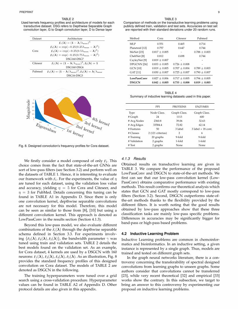
TABLE 2Used kernels frequency profiles and architecture of models for each

transductive dataset. DSG refers to Depthwise Separable Graphconvolution layer, G to Graph convolution layer, D to Dense layer

Dataset Architecture

z1(λ) = (1− λ/λmax)5

z3(λ) = exp(−0.25(0.25λmax − λ)2)

Cora z4(λ) = exp(−0.25(0.5λmax − λ)2)

z5(λ) = exp(−0.25(0.75λmax − λ)2)

DSG160-DSG7

Citeseer z1(λ) = (1− λ/λmax)5, z6(λ) = 1

DSG160-DSG6

Pubmed z1(λ) = (1− λ/λmax)3, z2(λ) = λ/λmax

DSG16-DSG3

Fig. 8. Designed convolution’s frequency profiles for Cora dataset.

We firstly consider a model composed of only z1. Thischoice comes from the fact that state-of-the-art GNNs aresort of low-pass filters (see Section 3.2) and perform well onthe datasets of TABLE 1. Hence, it is interesting to evaluateour framework with z1. For the experiments, the value of ηare tuned for each dataset, using the validation loss valueand accuracy, yielding η = 5 for Cora and Citeseer, andη = 3 for PubMed. Details concerning this tuning can befound in TABLE A1 in Appendix D. Since there is onlyone convolution kernel, depthwise separable convolutionsare not necessary for this model. Therefore, this modelcan be seen as similar to those from [8], [10] but using adifferent convolution kernel. This approach is denoted asLowPassConv in the results section (Section 4.1.3).

Beyond this low-pass model, we also evaluate differentcombinations of the zi(λ) through the depthwise separableschema defined in Section 3.3. For experiments involv-ing {z3(λ),z4(λ),z5(λ)}, the bandwidth parameter γ wastuned using train and validation sets. TABLE 2 details thebest models found on the validation set. As an example,for Cora dataset, 4 kernels are used by a DSGCN with 160neurons: z1(λ), z3(λ), z4(λ), z5(λ). As an illustration, Fig. 8provides the standard frequency profiles of this designedconvolution on Cora dataset. The models of TABLE 2 aredenoted as DSGCN in the following.

The training hyperparameters were tuned over a gridsearch using a cross-validation procedure. Hyperparametervalues can be found in TABLE A2 of Appendix D. Otherprotocol details are also given in this appendix.

TABLE 3Comparison of methods on the transductive learning problems usingpublicly defined train, validation and test sets. Accuracies on test setare reported with their standard deviations under 20 random runs.

Method Cora Citeseer Pubmed

MLP 0.551 0.465 0.714Planetoid [12] 0.757 0.647 0.744MoNet [23] 0.817 ± 0.005 - 0.788 ± 0.003ChebNet [8] 0.812 0.698 0.744CayleyNet [9] 0.819 ± 0.007 - -DPGCNN [26] 0.833 ± 0.005 0.726 ± 0.008 -GCN [10] 0.819 ± 0.005 0.707 ± 0.004 0.789 ± 0.003GAT [11] 0.830 ± 0.007 0.725 ± 0.007 0.790 ± 0.007

LowPassConv 0.827 ± 0.006 0.717 ± 0.005 0.794 ± 0.005DSGCN 0.842 ± 0.005 0.733 ± 0.008 0.819 ± 0.003

TABLE 4Summary of inductive learning datasets used in this paper.

PPI PROTEINS ENZYMES

Type Node Class. Graph Class. Graph Class.# Graph 24 1113 600# Avg.Nodes 2360.8 39.06 32.63# Avg.Edges 33584.4 72.82 62.14# Features 50 3 label 3 label + 18 cont.# Classes 2 (121 criterias) 2 6# Training 20 graphs 9-fold 9-fold# Validation 2 graphs 1-fold 1-fold# Test 2 graphs None None

4.1.3 ResultsObtained results on transductive learning are given inTABLE 3. We compare the performance of the proposedLowPassConv and DSGCN to state-of-the-art methods. Wefirst can see that our low-pass convolution kernel (Low-PassConv) obtains comparative performance with existingmethods. This result confirms our theoretical analysis whichstates that GCN and GAT mostly correspond to low-passfilters (Section 3.2). Second, DSGCN outperforms state-of-the-art methods thanks to the flexibility provided by thedifferent filters. It is worth noting that the good resultsobtained by low-pass approaches show that these threeclassification tasks are mainly low-pass specific problems.Differences in accuracies may be significantly bigger forband-pass or high-pass based problems.

4.2 Inductive Learning Problem

Inductive Learning problems are common in chemoinfor-matics and bioinformatics. In an inductive setting, a giveninstance is represented by a single graph. Thus, models aretrained and tested on different graph sets.

In the graph neural networks literature, there is a con-troversy concerning the transferability of spectral designedconvolutions from learning graphs to unseen graphs. Someauthors consider that convolutions cannot be transferred[23], while very recent theoretical [32] and empirical [33]works show the contrary. In this subsection, we target tobring an answer to this controversy by experimenting ourproposal on inductive learning problems.

PREPRINT 10

4.2.1 DatasetsInductive experiments are led on 3 datasets (see TABLE 4for a summary): a multi-graph node classification datasetcalled Protein-to-Protein Interaction (PPI) [34] and on twograph classification datasets called PROTEINS and EN-ZYMES [35]. The protocols used for the evaluations arethose defined in [11] for PPI and [36], [37], [38], [39] forPROTEINS and ENZYMES datasets.

The PPI dataset is a multi-label node classification prob-lem on multi-graphs. Each node has to be classified eitherTrue or False for 121 different criteria. All the nodes aredescribed by a 50-length continuous feature vector. ThePPI dataset includes 24 graphs, with a train/validation/teststandard splitting.

The PROTEINS and ENZYMES datasets are graph clas-sification datasets. There are 2 classes in PROTEINS and 6classes in ENZYMES. In PROTEINS dataset, there are threedifferent types of nodes and one continuous feature. But wedo not use this continuous feature on nodes. In ENZYMESdataset, there are 18 continuous node features and three dif-ferent kinds of node types. In the literature, some methodsuse all provided continuous node features while others useonly node label. This is why ENZYMES results are givenusing either all features (denoted by ENZYMES-allfeat) oronly node labels (denoted by ENZYMES-label).

Since there is no standard train, validation and testsets split for PROTEINS and ENZYMES, the results aregiven using a 10-fold cross-validation (CV) strategy under afixed predefined epoch number. The CV only uses trainingand validation set. Specifically, after obtaining 10 validationcurves corresponding to 10 folds, we first take average ofvalidation curves across the 10 folds and then select the sin-gle epoch that achieved the maximum averaged validationaccuracy. This procedure is repeated 20 times with randomseeds and random division of dataset. Mean accuracy andstandard deviation are reported. This is the same protocolthan [36], [37], [38], [39].

4.2.2 ModelsFor PPI, 7 depthwise graph convolution layers compose themodel. Each layer has 800 neurons, except the output layerwhich has 121 neurons, each one classifying the node eitherTrue or False. All layers use a ReLU activation except theoutput layer, which is linear. No dropout or regularizationof the binary cross-entropy loss function is used. All graphconvolutions use three spectral designed convolutions: alow-pass convolution given by z1(λ) = exp(−λ/10), ahigh-pass one given by z2(λ) = λ/λmax and an all-passfilter given by z3(λ) = 1.

For graph classification problems (PROTEINS and EN-ZYMES), depthwise graph convolution layers are notneeded since these datasets have a reduced number offeatures. Thus, it is tractable to use all multi-support graphconvolution layers instead of the depthwise schema. In thesecases, our models firstly consist of a series of graph convo-lution layers. Then, a global pooling (i.e., graph readout) isapplied in order to aggregate extracted features at graphlevel. For this pooling, we use a concatenation of meanand max global pooling operator, as used in [37]. Finally,a dense layer (except for ENZYMES-label) is applied, beforethe output layer as in [39].

TABLE 5Kernels frequency profiles and model architecture for each inductivedataset. meanmax refers to global mean and max pooling layer.

Same legend as TABLE 2.

Dataset Architecture

z1(λ) = exp(−λ/10)PPI z2(λ) = λ/λmax, z3(λ) = 1

DSG800-DSG800-DSG800-DSG800-DSG800-DSG800-DSG121

PROTEINS z1(λ) = 1− λ/λmax, z2(λ) = λ/λmax

G200-G200-meanmax-D100-D2

z1(λ) = 1, z2(λ) = λs − 1

ENZYMES-label z3(λ) = 2λ2s − 4λs + 1, λs = 2λ/λmax

G200-G200-G200-G200-meanmax-D6

z1(λ) = 1, z2(λ) = exp(−λ2)

ENZYMES-allfeat z3(λ) = exp(−(λ− 0.5λmax)2)

z4(λ) = exp(−(λ− λmax)2)

G200-G200-meanmax-D100-D6

TABLE 6Comparison of methods on inductive learning problems using publiclydefined data split for PPI dataset and 10-fold CV for PROTEINS andENZYMES datasets. PPI results are the test set results reported by

micro-F1 metric percentage. Others are CV results reported byaccuracy percentage. Results denoted by ∗ were reproduced from

original source codes but denoted feature set.

Method PPI PROTEINS ENZYMESAll Features Node Label Node Label All Features

GraphSAGE [22] 76.8 - - -GAT [11] 97.3 ± 0.20 - - -GaAN [40] 98.7 ± 0.20 - - -Hierarchical [37] - 75.46 64.17 -Diffpool [36] - 76.30 62.50 66.66∗

ChebNet [33] - 75.50 ± 0.40 58.00 ± 1.40 -Multigraph [33] - 76.50 ± 0.40 61.70 ± 1.30 68.00 ± 0.83GIN [39] - 76.20 ± 0.86 - -GFN [38] - 76.56 ± 0.30∗ 60.23 ± 0.92∗ 70.17 ± 0.86

MLP (C(1) = I) 46.2 ± 0.56 74.03 ± 0.92 27.83 ± 2.51 76.11 ± 0.87GCN (9) 59.2 ± 0.52 75.12 ± 0.82 51.33 ± 1.23 75.16 ± 0.65DSGCN 99.09 ± 0.03 77.28 ± 0.38 65.13 ± 0.65 78.39 ± 0.63

All details about the architecture and designed convolu-tions can be found in TABLE 5. The hyperparameters usedin best models can be found on TABLE A2 in Appendix D.

4.2.3 ResultsTABLE 6 compares the results obtained by the modelsdescribed above and state-of-the-art methods. A comparisonwith the same models but without graph information, aMulti-Layer Perceptron (MLP) that corresponds to C(1) = Iis also provided to discuss if structural data include in-formation or not. To the best of our knowledge, such ananalysis is not provided in the literature. Finally, resultsobtained by the same architecture with GCN kernel is alsoprovided.

As one can see in TABLE 6, the proposed method obtainscompetitive results on inductive datasets. For PPI, DSGCNclearly outperforms state-of-the-art methods with the sameprotocol, reaching a micro-F1 percentage of 99.09 and an ac-curacy of 99.45%. For this dataset, MLP accuracy is low since

PREPRINT 11

the percentage of micro-F1 is 46.2 (random classifier’s micro-F1 being 39.6%). This means that the problem includessignificant structural information. Using the GCN kernel,which operates as low-pass convolution (see Section 3.2),the accuracy increases to 0.592, but again not comparablewith state-of-the-art accuracy.

For the PROTEINS dataset, one can see that MLP (C(1) =I) reaches an accuracy that is quite comparable with state-of-the-art GNN methods. Hence, MLP reaches a 74.03%validation accuracy while the proposed DSGCN reaches77.28%, which is the best performance among GNNs. Thismeans that PROTEINS problem includes very few structuralinformation to be exploited by GNNs.

ENZYMES dataset results are very interesting in order tounderstand the importance of continuous features and theirprocessing through different convolutions. As one can seein TABLE 6, there are important differences of performancebetween the results on ENZYMES-label and ENZYMES-allfeat. When node labels are used alone, without features,MLP accuracy is very poor and nearly acts as a randomclassifier. When using all features, MLP outperforms GCNand even some state-of-the-art methods. A first explanationis that methods are generally optimized for just node labelbut not for continuous features. Another one is that thecontinuous features already include information related tothe graph structure since they are experimentally measured.Hence, their values are characteristic of the node whenit is included in the given graph. Since GCN is just alow-pass filter, it removes some important information onhigher frequency and decreases the accuracy. Thanks to themultiple convolutions proposed in this paper, our GNN DS-GCN clearly outperforms other methods on the ENZYMESdataset.

5 CONCLUSION

The success of convolutions in neural network stronglydepends on the capability of defined convolution kernelson producing outputs as different as possible. While thishas been widely investigated for CNNs, there has not beenany study for ConvGNNs with graph convolution, to thebest of our knowledge. This paper proposed to fill this gap,by examining the graph convolutions as custom frequencyprofiles and taking advantage of using optimized multi-frequency profile convolutions. By this way, we significantlyincreased the performance on reference datasets.

Nevertheless, the proposed approach has some draw-backs. First, it needs eigenvalues and eigenvectors of thegraph Laplacian. If the graph has more than 20k nodes,computing these values is not tractable. Second, we didnot propose yet any automatic procedure to select thebest frequency profile of convolution. Hence, the proposedapproach needs expertise to find the appropriate graphkernels. Third, although our theoretic complexity is thesame than GCN or ChebNet, in practice our convolutionsare more dense than GCN, which makes it slower in practicesince it cannot take advantage of sparse matrix multipli-cations. Last, if edge type can be handled by designingconvolution for each type, the proposed method does nothandle continuous edge features and directed edges.

Our future work will target the automatic design ofgraph convolutions in spectral domain. It may be done byunsupervised manner as preprocessing step. Another futurework will be on handling given continuous edge featuresand directed edge in our framework. Also, we have a planto design convolution frequencies not by function of eigen-values but through linear combination of Chebyshev kernelsin order to skip the necessity of eigenvalue calculations.

ACKNOWLEDGMENTS

This work was partially supported by the ANR grant APi(ANR-18-CE23-0014), the Normandy Region project AGACand the PAUSE Program.

REFERENCES

[1] A. Krizhevsky, I. Sutskever, and G. E. Hinton, “Imagenet classifi-cation with deep convolutional neural networks,” in NIPS, 2012.

[2] A. Graves, A.-r. Mohamed, and G. Hinton, “Speech recognitionwith deep recurrent neural networks,” in 2013 IEEE internationalconference on acoustics, speech and signal processing. IEEE, 2013, pp.6645–6649.

[3] F. Scarselli, M. Gori, A. C. Tsoi, M. Hagenbuchner, and G. Mon-fardini, “The graph neural network model,” IEEE Transactions onNeural Networks, vol. 20, no. 1, pp. 61–80, December 2009.

[4] J. Gilmer, S. S. Schoenholz, P. F. Riley, O. Vinyal, and G. E. Dahl,“Neural message passing from quantum chemistry,” in Proceedingsof the International Conference on Machine Learning, 2017.

[5] M. M. Bronstein, J. Bruna, Y. LeCun, A. Szlam, and P. Van-dergheynst, “Geometric deep learning: Going beyond euclideandata,” IEEE Signal Processing Magazine, vol. 34, no. 4, pp. 18–42,July 2017.

[6] Z. Wu, S. Pan, F. Chen, G. Long, C. Zhang, and P. S. Yu, “Acomprehensive survey on graph neural networks,” arXiv preprintarXiv:1901.00596, 2019.

[7] J. Bruna, W. Zaremba, A. Szlam, and Y. LeCun, “Spectral net-works and locally connected networks on graphs,” arXiv preprintarXiv:1312.6203, 2013.

[8] M. Defferrard, X. Bresson, and P. Vandergheynst, “Convolutionalneural networks on graphs with fast localized spectral filtering,”in Advances in Neural Information Processing Systems, 2016, pp.3844–3852.

[9] R. Levie, F. Monti, X. Bresson, and M. M. Bronstein, “Cayleynets:Graph convolutional neural networks with complex rational spec-tral filters,” IEEE Transactions on Signal Processing, vol. 67, no. 1,pp. 97–109, Jan 2019.

[10] T. N. Kipf and M. Welling, “Semi-supervised classification withgraph convolutional networks,” in International Conference onLearning Representations (ICLR), 2017.

[11] P. Velickovic, G. Cucurull, A. Casanova, A. Romero, P. Lio, andY. Bengio, “Graph attention networks,” in International Conferenceon Learning Representations (ICLR), 2018.

[12] Z. Yang, W. W. Cohen, and R. Salakhutdinov, “Revisiting semi-supervised learning with graph embeddings,” in Proceedings of the33rd International Conference on International Conference on MachineLearning, ICML’16, 2016.

[13] Z. Wu, S. Pan, F. Chen, G. Long, C. Zhang, and P. S. Yu, “Acomprehensive survey on graph neural networks,” arXiv preprintarXiv:1901.00596, 2019.

[14] F. Chung, Spectral graph theory. American Mathematical Society,1997.

[15] D. I. Shuman, S. K. Narang, P. Frossard, A. Ortega, and P. Van-dergheynst, “The emerging field of signal processing on graphs:Extending high-dimensional data analysis to networks and otherirregular domains,” IEEE signal processing magazine, vol. 30, no. 3,pp. 83–98, 2013.

[16] M. Henaff, J. Bruna, and Y. LeCun, “Deep convolutional networkson graph-structured data,” arXiv preprint arXiv:1506.05163, 2015.

[17] S. Kearnes, K. McCloskey, M. Berndl, V. Pande, and P. Riley,“Molecular graph convolutions: moving beyond fingerprints,”Journal of computer-aided molecular design, vol. 30, no. 8, pp. 595–608, 2016.

PREPRINT 12

[18] D. K. Duvenaud, D. Maclaurin, J. Iparraguirre, R. Bombarell,T. Hirzel, A. Aspuru-Guzik, and R. P. Adams, “Convolutional net-works on graphs for learning molecular fingerprints,” in Advancesin Neural Information Processing Systems, 2015, pp. 2224–2232.

[19] M. Niepert, M. Ahmed, and K. Kutzkov, “Learning convolutionalneural networks for graphs,” in Proceedings of the InternationalConference on Machine Learning, 2016, pp. 2014–2023.

[20] Y. Hechtlinger, P. Chakravarti, and J. Qui, “A generalization ofconvolutional neuralnetworks to graph-structured data,” arXivpreprint arXiv:1704.08165, 2017.

[21] J. Atwood and D. Towsley, “Diffusion-convolutional neural net-works,” in Advances in Neural Information Processing Systems, 2016,pp. 1993–2001.

[22] W. Hamilton, Z. Ying, and J. Leskovec, “Inductive representationlearning on large graphs,” in Advances in Neural Information Pro-cessing Systems, 2017, pp. 1024–1034.

[23] F. Monti, D. Boscaini, J. Masci, E. Rodola, J. Svoboda, and M. M.Bronstein, “Geometric deep learning on graphs and manifoldsusing mixture model cnns,” in Proceedings of the IEEE Conferenceon Computer Vision and Pattern Recognition, 2017, pp. 5115–5124.

[24] M. Fey, J. Eric Lenssen, F. Weichert, and H. Muller, “Splinecnn:Fast geometric deep learning with continuous b-spline kernels,”in Proceedings of the IEEE Conference on Computer Vision and PatternRecognition, 2018, pp. 869–877.

[25] B. Xu, N. Wang, T. Chen, and M. Li, “Empirical evaluationof rectified activations in convolutional network,” arXiv preprintarXiv:1505.00853, 2015.

[26] F. Monti, O. Shchur, A. Bojchevski, O. Litany, S. Gunnemann, andM. M. Bronstein, “Dual-primal graph convolutional networks,”2018.

[27] D. K. Hammond, P. Vandergheynst, and R. Gribonval, “Waveletson graphs via spectral graph theory,” Applied and ComputationalHarmonic Analysis, vol. 30, no. 2, pp. 129–150, 2011.

[28] M. Zhang, Z. Cui, M. Neumann, and Y. Chen, “An end-to-enddeep learning architecture for graph classification,” in Thirty-Second AAAI Conference on Artificial Intelligence, 2018.

[29] S. Abu-El-Haija, B. Perozzi, A. Kapoor, H. Harutyunyan,N. Alipourfard, K. Lerman, G. V. Steeg, and A. Galstyan, “Mixhop:Higher-order graph convolution architectures via sparsified neigh-borhood mixing,” in International Conference on Machine Learning(ICML), 2019.

[30] F. Chollet, “Xception: Deep learning with depthwise separableconvolutions,” in Proceedings of the IEEE conference on computervision and pattern recognition, 2017, pp. 1251–1258.

[31] M. Sandler, A. G. Howard, M. Zhu, A. Zhmoginov, and L. Chen,“Mobilenetv2: Inverted residuals and linear bottlenecks,” in 2018IEEE Conference on Computer Vision and Pattern Recognition, CVPR2018, Salt Lake City, UT, USA, June 18-22, 2018. IEEE ComputerSociety, 2018, pp. 4510–4520.

[32] R. Levie, E. Isufi, and G. Kutyniok, “On the transferability ofspectral graph filters,” arXiv preprint arXiv:1901.10524, 2019.

[33] B. Knyazev, X. Lin, M. R. Amer, and G. W. Taylor, “Spectralmultigraph networks for discovering and fusing relationships inmolecules,” arXiv preprint arXiv:1811.09595, 2018.

[34] M. Zitnik and J. Leskovec, “Predicting multicellular functionthrough multi-layer tissue networks,” Bioinformatics, vol. 33,no. 14, pp. i190–i198, 2017.

[35] K. Kersting, N. M. Kriege, C. Morris, P. Mutzel, and M. Neu-mann, “Benchmark data sets for graph kernels,” 2016, http://graphkernels.cs.tu-dortmund.de.

[36] Z. Ying, J. You, C. Morris, X. Ren, W. Hamilton, and J. Leskovec,“Hierarchical graph representation learning with differentiablepooling,” in Advances in Neural Information Processing Systems,2018, pp. 4800–4810.

[37] C. Cangea, P. Velickovic, N. Jovanovic, T. Kipf, and P. Lio,“Towards sparse hierarchical graph classifiers,” arXiv preprintarXiv:1811.01287, 2018.

[38] Y. S. Ting Chen, Song Bian, “Dissecting graph neural networks ongraph classification,” CoRR, vol. abs/1905.04579, 2019.

[39] K. Xu, W. Hu, J. Leskovec, and S. Jegelka, “How powerful aregraph neural networks?” in International Conference on LearningRepresentations, 2019.

[40] J. Zhang, X. Shi, J. Xie, H. Ma, I. King, and D.-Y. Yeung, “Gaan:Gated attention networks for learning on large and spatiotemporalgraphs,” in Conference on Uncertainty in Artificial Intelligence, UAI,2018.

Muhammet Balcilar is a postdoctoral re-searcher at LITIS Lab, University of Rouen Nor-mandy. He received his B.S., M.S. and Ph.D. de-grees in Computer Engineering from Yıldız Tech-nical University, Istanbul in 2005, 2007 and 2013respectively. Machine Learning, Image Process-ing and Robotics are the major research areasof the researcher.

Guillaume Renton started his PHD at the Litislaboratory in the university of Rouen in 2017.His research interest are machine learning,deep neural network and their applications overgraphs.

Pierre Heroux obtained his PhD from the Uni-versity of Rouen in 2001. Since 2001, he isan assistant professor in the Learning Teamof LITIS at University of Rouen. His currentresearch interests include the development ofpattern recognition methods for graphs with afocus on subgraph isomorphism, integer linearprogramming for the computation/approximationof graph edit distance and metric learning ongraphs by means of deep architectures.

Benoit Gauzere obtained his phD from Univer-sity of Caen in 2013 on the definition of graphkernels for chemoinformatics. Since 2015, he’san assistant professor in the App team of INSARouen Normandie and LITIS lab.

Sebastien Adam is full Professor at the LITISlab in Rouen, Normandy University, France. Hisdomains of interest are at the merging of ma-chine learning and graph-based pattern recogni-tion with applications in document image analy-sis.

Paul Honeine (M’07) obtained in 2007 his Ph.D.degree in Systems Optimisation and Securityfrom the University of Technology of Troyes,France, and was a Postdoctoral Research as-sociate with the Systems Modeling and De-pendability Laboratory, from 2007 to 2008. FromSeptember 2008 till August 2015, he was an as-sistant Professor at the University of Technologyof Troyes, France. Since September 2015, he isfull professor at the LITIS Lab of the Universityof Rouen (Normandie Universite), France.

PREPRINT 13

Bridging the Gap Between Spectral and Spatial Domains in Graph Neural Networks

Muhammet Balcilar, et al.

APPENDIX ATHEORETICAL ANALYSIS OF CHEBYSHEV KERNELSFREQUENCY PROFILE

In this appendix, we provide the expressions of the full andstandard frequency profiles of the Chebyshev convolutionkernels.

Theorem A.1. The frequency profile of the first Chebyshevconvolution kernel for any undirected arbitrary graph defined byC(1) = I can be defined by

z1(λ) = 1, (22)

where 1 denotes the vector of ones of appropriate size.

Proof: When the identity matrix is used as convolu-tion kernel, it just directly transmits the inputs to the outputswithout any modification. This process is called all-passfilter. Mathematically, we can calculate the full frequencyprofile for kernel I by using Corollary 1.1, namely

z1 = U>IU = U>U = I, (23)

since the eigenvectors are orthonormal. Therefore, we canparameterize the diagonal of the full frequency profile by λand reach the standard frequency profile as follows:

z1(λ) = diag(I) = 1. (24)

Theorem A.2. The frequency profile of the second Chebyshevconvolution kernel for any undirected arbitrary graph given byC(2) = 2L/λmax − I can be defined by

z2(λ) =2λ

λmax− 1. (25)

Proof: We can compute the C(2) kernel full frequencyprofile using Corollary 1.1:

z2 = U>(

2

λmaxL− I

)U. (26)

Since U>IU = I , (26) can be rearranged as

z2 =2

λmaxU>LU − I. (27)

Since λ = [λ1, . . . , λn] are the eigenvalues of the graphLaplacian L, those must conform to the following condition:

LU = U diag(λ); (28)U>LU = diag(λ). (29)

Replacing (29) into (27), we get

z2 =2

λmaxdiag(λ)− I. (30)

This full frequency profile consists of two parts, a diagonalmatrix and the negative identity matrix. Therefore, we can

parameterize the full frequency matrix diagonal to show thestandard frequency profile as follows:

z2(λ) = diag(z2) =2λ

λmax− 1. (31)

Theorem A.3. The frequency profile of third and followingsChebyshev convolution kernels for any undirected arbitrary graphcan be defined by

zk = 2z2zk−1 −zk−2, (32)

and their standard frequency profiles by

zk(λ) = 2z2(λ)zk−1(λ)−zk−2(λ). (33)

Proof: Given the third and following Chebyshev ker-nels defined by C(k) = 2C(2)C(k−1) − C(k−2) and usingCorollary 1.1, the corresponding frequency profile is

zk = U>(

2C(2)C(k−1) − C(k−2))U. (34)

By expanding (34), we get

zk = 2U>C(2)C(k−1)U − U>C(k−2)U. (35)

Since UU> = I , we can insert the product UU> into (35).Thus, we have

zk = 2U>C(2)UU>C(k−1)U − U>C(k−2)U (36)

zk = 2(U>C(2)U

)(U>C(k−1)U

)− U>C(k−2)U. (37)

Since zk′ = U>C(k′)U for any k′, it follows that (37) and(32) are identical.

Hence z1 and z2 are diagonal matrices, and the rest ofthe kernels frequency profiles become diagonal matrices in(32). Therefore, we can write the corresponding standardfrequency profiles of third and followings Chebyshev con-volution kernels as follows:

zk(λ) = 2z2(λ)zk−1(λ)−zk−2(λ). (38)

APPENDIX BTHEORETICAL ANALYSIS OF CAYLEYNET FRE-QUENCY PROFILE

CayleyNet uses in (2) the weight vector parametrizationFi,j,l = [gi,j,l(λ1, h), ..., gi,j,l(λn, h)]>, where the functiong(·, ·) is defined in [9] by

g(λ, h) = c0 + 2Re

(r∑

k=1

ck

(hλ− ıhλ+ i

)k), (39)

where i2 = −1, Re(·) is the function that returns the realpart of a given complex number, c0 is a trainable real coef-ficient, and c1, . . . , cr are complex trainable coefficients. We

PREPRINT 14

can write hλ − i in Euler form by√h2λ2 + 1.ei atan2(−1,hλ)

and for hλ + i by√h2λ2 + 1.ei atan2(1,hλ). By this substitu-

tion, (39) becomes

g(λ, h) = c0 + 2Re

(r∑

k=1

ckeik(atan2(−1,hλ)−atan2(1,hλ))

).

(40)where atan2(y, x) is the inverse tangent function, whichfinds the angle (in range of [−π, π]) of a point given its y andx coordinates. For further simplification, let us introduce theθ(·) function defined by

θ(x) = atan2(−1, x)− atan2(1, x). (41)

Since the cks are complex numbers, we can write them asa sum of real and imaginary parts, ck = ak/2 + ibk/2 (thescale factor 2 is added for convenience). Thus, (40) can berewritten as follows:

g(λ, h) = c0 +Re

(r∑

k=1

(ak + ibk)eikθ(hλ)

). (42)

We can replace eikθ(hλ) with its polar coordinate equiva-lence form cos(kθ(hλ)) + i sin(kθ(hλ)). When we removethe imaginary components because of Re(·) function, (42)becomes

g(λ, h) = c0 +r∑

k=1

ak cos(kθ(hλ))− bk sin(kθ(hλ)). (43)

In this definition, there is no complex coefficient, but onlyreal coefficients (c0, ak and bk for k = 1, . . . , r) to be tunedby training. By using the form in (43), we can parametrizeCayleyNet by the parametrization matrix B ∈ Rn×2r+1, asin (3), by

[g(λ0, h), . . . , g(λn, h)]> = B[c0, a1, b1, . . . , ar, br]>. (44)

The s-th column vector of matrix B, denotes Bs, must fulfillthe following conditions:

Bs = zs(λ) =

1 if s = 1cos( s2θ(hλ)) if s ∈ {2, 4, . . . , 2r}− sin( s−12 θ(hλ)) if s ∈ {3, 5, . . . , 2r + 1}

(45)We can see CayleyNet as a spectral graph convolution thatuses 2r + 1 convolution kernels. The first kernel is anall-pass filter, and the frequency profiles of remaining 2rkernels (zs(λ)) are created using sine and cosine functions,with a parameter h used to scale the eigenvalues in (45).Considering (12) in Theorem 1, we can write CayleyNet’sconvolutions (C(s)) in spatial domain. CayleyNet includesthe tuning of this scaling parameter in the training pipeline.Note that because of the function definition in (41), θ(hλ) isnot linear in λ. Therefore, zs cannot be a perfect sinusoidalin λs.

APPENDIX CTHEORETICAL ANALYSIS OF GCN FREQUENCYPROFILE

In this appendix, we study the GCN and its convolutionkernel. We start by deriving the expression of its frequencyprofile.

Theorem C.1. The frequency profile of GCN convolution kernelis defined by

CGCN = D−1/2AD−1/2, (46)

and can be written as

zGCN (λ) = 1− p

p+ 1λ, (47)

where λ is the eigenvalues of the normalized graph Laplacian andthe given graph is an undirected regular graph whose node degreesare all equal to p.

Proof: Since Di,i =∑j Ai,j and A = (A+ I), we can

rewrite (46) as:

CGCN = (D + I)−1/2(A+ I)(D + I)−1/2. (48)

Under the assumption that all node degrees are equal to p,we can write the diagonal degree matrix by D = pI . Then,(48) can be rewritten as

CGCN = ((p+ 1)I)−1/2(A+ I)((p+ 1)I)−1/2, (49)

which is equivalent to

CGCN =A+ I

p+ 1. (50)

Using Corollary 1.1, we can express the frequency profile ofCGCN in matrix form by

zGCN =1

p+ 1U>AU +

1

p+ 1I. (51)

Since λ = [λ1, . . . , λn] are the eigenvalues of the normalizedgraph Laplacian L = I−D−1/2AD−1/2, they must conformto the following condition:(

I −D−1/2AD−1/2)U = U diag(λ). (52)

According to D = pI , it conforms to D−1/2AD−1/2 = A/p.Thus, (52) can be written as

U − AU

p= U diag(λ). (53)

Then AU is expressed as

AU = pU − pU diag(λ) (54)

Replacing AU in (51), we obtain

zGCN =1

p+ 1U> (pU − pU diag(λ)) +

1

p+ 1I. (55)

Since U>U = I , then we have

zGCN =pI − p diag(λ) + I

p+ 1. (56)

This expression can be simplified to

zGCN = I − p

p+ 1diag(λ), (57)

which is equal to the matrix form defined in (47) sincezGCN (λ) = diag(zGCN ).

This demonstration shows that the GCN frequency pro-file acts as a low-pass filter. When the given graph is acircular undirected graph, all node degrees are equal top = 2, leading to a frequency profile defined by 1 − 2λ/3.Since the normalized graph Laplacian eigenvalues are in the

PREPRINT 15

range [0, 2], the filter magnitude linearly decreases until thethird quarter of the spectrum (cut-off frequency) where itreaches zero. Then it linearly increases until the end of thespectrum. This explains the shape of the frequency profile ofGCN convolutions for 1D regular graph observed in Fig. 4.

However, this conclusion cannot explain the perturba-tions on the GCN frequency profile. To analyse this point,we relax the assumption D = pI and rewrite (48) as

CGCN = (D + I)−1 + (D + I)−1/2A(D + I)−1/2. (58)

We can see that the GCN kernel consists of two parts,CGCN = c1 +c2, where first part is given by c1 = (D+I)−1

and the second one is c2 = (D + I)−1/2A(D + I)−1/2.For the second part (c2), we can write it using the

element-wise multiplication operator � (Hadamard multi-plication)

c2 = A�√1/(d+ 1) ·

√1/(d+ 1)

>, (59)

where d is the column degree vector d = diag(D) and thedivision and square-root are also element-wise (Hadamard)operations. With the same notation, we can rewrite theChebyshev second kernel, assuming that λmax = 2,

C(2) = −A�√1/d ·

√1/d

>. (60)

The two expressions (59) and (60) show that negative c2 isan approximation of the second Chebyshev kernel if vectord consists of same values, as it was assumed in Theorem C.1.When the vector d is composed of different values, the twomatrices

√1/d.

√1/d

>and

√1/(d+ 1).

√1/(d+ 1)

>are

not proportional for each coordinate (i.e., entry). To obtainc2 from C(2), we need to use different coefficients for eachcoordinate of the kernel. If the difference between nodedegrees is important, these coefficients have the strong in-fluence, and c2 may be very different from C(2). Conversely,if the node degrees are quite uniform, these coefficientsmay be neglected. This phenomenon is the first cause ofperturbation on GCN frequency profile.

The first part (c1) of the GCN kernel in (58) is moreinteresting. Actually, it is a diagonal matrix that showsthe contribution of each node in the convolution process.Instead of looking for some approximations of known fre-quency profiles such as those of Chebyshev kernels, we canwrite its frequency profile directly. Using Corollary 1.1, wecan express the frequency profile of c1 in matrix form by

zc1 = (U>c1 U), (61)

where U is the eigenvectors matrix. By taking advantage ofhaving a diagonal kernel c1, we can express each componentof full frequency profile as

zc1(i, j) =n∑k=1

(1

1 + dkUi,kUj,k

), (62)

where n is the number of nodes in the graph, dk is degree ofthe k-th node, Ui,k is the k-th element of i-th eigenvector. Aseigenvectors Ui and Uj are orthogonal for i 6= j, their scalarproduct is null. However, in (62), the weighting coefficient

11+dk

is not constant over all the dimensions of the eigen-vectors. Therefore, there is no guarantee that zc1(i, j) is null.

This is another reason that explains that the GCN frequencyprofile has many non-zero elements outside of the diagonal.

In addition, it is also clear that the standard frequencyprofile of c1 (diagonal of zc1 , i.e., zc1(i, i) in (62)) is notsmooth. Indeed, the diagonal elements of zc1 can be writtenas a weighted sum of squared eigenvalues elements, whichagain is weighted by 1/(1 + dk). If the latter is constantfor all k, the sum of squared eigenvectors elements has tobe 1 since the eigenvectors have unit L2-norm. But in thegeneral case where 1/(1 + dk) are not necessarily constantover all the dimensions of eigenvectors, the diagonal of thematrix may have some perturbations. This point constitutesanother explanation on the fact that the GCN standardfrequency profile is not smooth.

On the other hand, under the assumption that the nodedegrees distribution is uniform, we can derive the followingapproximation:

p ≈ d =1

n

n∑k=1

dk. (63)

We can then write an approximation of the GCN frequencyprofile as a function of the average node degree by replacingp with d in (54) and obtain the final approximation:

zGCN (λ) ≈ 1− d

d+ 1λ. (64)

We can theoretically show the cut-off frequency where GCNkernel’s frequency profile reach 0 by

λcut ≈d+ 1

d. (65)

APPENDIX DAPPLICATION DETAILS

This section presents some additional details on the experi-mental settings and parameter tuning.

In the experiments of transductive learning problems,we tuned single convolution low-pass filter’s parameter η inz1(λ) = (1 − λ/λmax)η . TABLE A1 shows searching spaceof η and their loss and accuracy performance over differentdatasets. One can see that we decided to use η = 5 forCora and Citeseer, and η = 3 for PubMed dataset where itmaximizes the validation set performance.

TABLE A1Minimum validation set loss value and maximum validation set

accuracy over different low-pass filters.

Convolution Cora Citeseer PubMedz1(λ) Loss Acc Loss Acc Loss Acc

(1− λ/λmax)1 1.116 80.4 1.12 73.0 0.654 77.1(1− λ/λmax)3 0.745 81.8 1.02 72.6 0.572 81.1(1− λ/λmax)5 0.705 81.8 1.02 73.8 0.592 80.5(1− λ/λmax)10 0.752 81.2 1.01 72.2 - -(1− λ/λmax)20 0.792 80.8 1.01 71.2 - -

In depthwise separable graph convolution layer, theinitialization of the trainable parameters w(s,l) affects theperformance. If designed convolutions are supposed tohave equal effect on the model, these parameters can be

PREPRINT 16

TABLE A2Used hyperparameters.

Hyperparameters Cora Citeseer PubMed PPI PROTEINS ENZYMES-label ENZYMES-allfeatHidden Activations ReLU ReLU ReLU ReLU ReLU ReLU ReLUOutput Activation Linear Linear ReLU Linear Linear Linear LinearHidden Biases False False False True False False FalseOutput Bias True True False True True True TrueInput Dropout 0.75 0.75 0.25 0 0 0.1 0.1Kernel Dropout 0.75 0.75 0 0 0 0.1 0.1Weight Decay 3e-4 3e-4 5e-4 0 0 1e-4 1e-4Weight Decay on DSG 3e-3 3e-3 5e-3 0 - - -Learning Coeff 0.01 0.01 0.01 0.01 0.0005 0.001 0.001Batch Size 1 1 1 1 333 180 180Epoch 400 100 250 500 100 500 500

initialized randomly. But, if one is supposed to have moreeffect on the model, the important convolution kernel’scorrespondence weights can be initialized by 1, the restof them initialized by 0. In our model, we assumed thefirst kernel is always the most important kernel. Thus, weinitialized the first kernel’s depthwise separable weights asw(1,l) = 1, and the rest of the kernel’s depthwise separableweights w(s,l) = 0 when s > 1. In this way, the model startstraining as there is only kernel, which is supposed to be themost important one.

The used hyperparameters in our experiments are pre-sented in Table A2. We applied softmax to the outputof the models and calculate cross entropy loss functionfor all problems expect PPI dataset. Since PPI is two classclassification problem and we coded output by one neuron,we applied tansig to the output of the PPI model and usedbinary cross entropy as loss function. In our models we didnot consider any regularization on the bias parameter, butwe applied the L2-loss to the trainable weights. In the depth-wise separable layer, there are two different kinds of weightswhere additional one is depthwise weights. That is why inTABLE A2, there is two different weight decays. We alwaysused ReLU activation on the hidden layers and the Linearfor output layers. The table also provides if bias values areused in the hidden and output layers. In our model, weused two different types of dropout: the dropout applied onthe inputs of the layer as usually used in the literature, andthe dropout applied on the convolution kernel, which wasfirst used in [11] according to the best of our knowledge.Since Cora, Citeseer and PubMed datasets consist of onesingle graph, batch size is 1 for these problems. For the PPIdataset of only 24 graphs, we still prefer to update the modelfor each training graph. But for PROTEINS and ENZYMESdatasets, we update the model 3 times in each epoch. Sincein PROTEINS there are 1113 graphs and in each fold thereare 1000 graphs in the train set, we used a 333 batch size.As the same in ENZYMES there is 540 graphs in each trainfold, we used a 180 batch size to update the model 3 timesin a single epoch. We used the Adam optimization and afixed learning-coefficient in all models. The used learningcoefficient and the maximum epoch number can be foundin the Table A2.