
Breach, Remedies and Dispute Settlement in Trade … Remedies and Dispute Settlement in Trade...
55
Breach, Remedies and Dispute Settlement in Trade Agreements ∗ Giovanni Maggi Yale University and NBER Robert W. Staiger Stanford University and NBER March 2009 (Preliminary) Abstract We analyze the optimal design of legal remedies for breach in the context of inter- national trade agreements. Our formal analysis delivers sharp normative conclusions concerning the appropriate remedy for breach and optimal institutional design in light of features of the underlying economic and contracting environment. And our analysis also delivers novel positive predictions regarding when disputes arise in equilibrium, and how the disputes are resolved. ∗ We thank Chad Bown, Petros C. Mavroidis and participants in the Stanford Seminar on Dispute Settlement for very helpful comments.
Transcript of Breach, Remedies and Dispute Settlement in Trade … Remedies and Dispute Settlement in Trade...

Breach, Remedies and Dispute Settlement inTrade Agreements∗
Giovanni Maggi
Yale University and NBER
Robert W. Staiger
Stanford University and NBER
March 2009 (Preliminary)
Abstract
We analyze the optimal design of legal remedies for breach in the context of inter-
national trade agreements. Our formal analysis delivers sharp normative conclusions
concerning the appropriate remedy for breach and optimal institutional design in light
of features of the underlying economic and contracting environment. And our analysis
also delivers novel positive predictions regarding when disputes arise in equilibrium, and
how the disputes are resolved.
∗We thank Chad Bown, Petros C. Mavroidis and participants in the Stanford Seminar on Dispute Settlementfor very helpful comments.

1. Introduction
When governments make international commitments, what should be the legal remedy for
breach under their agreement? Should a government who is harmed by the breach be able to
demand specific performance of the commitment under the law, or simply the payment of dam-
ages for the harm done? In this paper we address these questions as they arise in the context
of international trade agreements. Our analysis delivers normative conclusions concerning the
appropriate remedy for breach and optimal institutional design in light of features of the un-
derlying economic and contracting environment, and it delivers a rich set of positive predictions
regarding when disputes arise in equilibrium and how the disputes are resolved.
We pay particular attention to the World Trade Organization (WTO) and the General
Agreement on Tariffs and Trade (GATT), its predecessor agreement. While this is a natural
institution on which to focus, given its prominence in the world trading system, we emphasize
that our analysis applies to international trade agreements more generally — and indeed even
to agreements outside the trade policy area.
In the WTO (and GATT before it), the central international commitments made by gov-
ernments relate to market access,1 and answers to the questions posed above help to define the
nature of the entitlements over access to foreign markets that governments can secure for their
exporters by contracting with other governments. Two related issues can be identified. A first
issue concerns the design of dispute settlement procedures and the mandate of the Dispute Set-
tlement Body (DSB). When the terms of the contract are breached, should the DSB if invoked
be asked to enforce contract performance? Or should it rather be asked to specify a level of
damages and allow a choice between performance or a damage payment and breach? A second
issue concerns the design of escape clauses built in to the terms of the contract itself: When
should an escape clause be made available, and what should a government be legally obliged to
pay in order to exercise it?
Behind these issues lies the important possibility that governments may bargain to settle
their differences without recourse to a DSB ruling: in this case the legal rules and remedies will
not directly determine the outcome, but they will indirectly impact the outcome by shaping
what governments can expect if their attempts at settlement fail. And in the presence of
transaction costs, these legal rules and remedies can have important efficiency consequences
1The only WTO commitments that do not derive their purpose from market access concerns are those related
to intellectual property rights protection and found in the TRIPs agreement.
1
even when bargaining and settlement is the dominant outcome.
Analogous questions and issues have been extensively studied in a domestic context as they
relate to the actions of private agents in two related literatures in law and economics. A funda-
mental question in the literature concerned with domestic contracts (see, for example, Schwartz,
1979, Ulen, 1984, and Shavell, 2006) is when contracting parties would want specific perfor-
mance and when they would instead prefer damage payments as a remedy for contract breach.
There is also a vast literature (see, for example, Calabresi and Melamed, 1972, and Kaplow
and Shavell, 1996) that is concerned with the related question of when property rules, under
which an entitlement can only be removed from its holder through a voluntary transaction,
are preferred to liability rules, whereby the entitlement can be removed from its holder for the
payment of objectively determined damages.
In the domestic context that is the focus of these literatures, the transaction costs that
underlie the efficiency consequences of the choice of legal rules are typically associated with
private information or other bargaining frictions. Such frictions are surely present as well in
international bargaining, but in the international context there is an additional feature that
is particularly salient and that distinguishes the international environment from its domestic
counterpart: in the international government-to-government setting, there generally do not ex-
ist efficient transfer mechanisms that can be used to make damage payments, either to settle
disputes or to compensate for the exercise of escape clauses. In the GATT/WTO, the typ-
ical means by which one government achieves compensation for the harm done by another
government’s actions is through “counter-retaliation,” that is, by raising its own tariffs above
previously negotiated levels. Such compensation mechanisms entail important inefficiencies
(deadweight loss) that, while plausibly absent in the domestic private agent context, introduce
a novel transaction cost in the international context through which the choice of legal rules and
remedies can have efficiency consequences.2
A major point of departure of our model is precisely this difference between the domestic
private agent setting and the international government-to-government setting. In particular, we
2Other possible means of compensation are a reduction of trade barriers in other sectors by the breaching
government, or changes in non-trade policies. Both of these mechanisms are likely to entail deadweight losses.
Even with cash transfers between governments, which are extremely rare in the context of the settlement of trade
disputes (see note 4), the revenue must still be collected, and unless lump-sum tax instruments are available to
governments these transfer mechanisms will have efficiency costs too. Our point here is simply that, unlike in
the domestic privet-agent context, the transfer mechanisms available to governments will often entail important
efficiency costs (see, however, note 6).
2

consider a setting where governments, operating in the presence of ex-ante uncertainty about
the joint benefits of free trade (which could be positive or negative, due to the possible presence
of political-economy factors), contract over trade policy and define a mandate for the DSB in
the event that contract disputes should arise ex post, once uncertainty has been resolved and
trade policies are chosen. We assume that transfers between governments are costly and that the
marginal cost of transfers is (weakly) increasing in the magnitude of the transfer. And finally, to
highlight the implications of costly transfers, we abstract from the ex-post bargaining frictions
that are typically emphasized in the domestic context.
We consider agreements that specify a baseline commitment to free trade but allow the
importing government to escape (breach) this commitment by compensating the exporter with
a certain amount of damages. If the level of damages is set either at zero or at a level so high
that the importing government would never choose to breach, then we may interpret this as a
property rule in which either the entitlement to protect is assigned to the importing government
or the entitlement to free trade is assigned to the exporting government. Alternatively, if
damages are set at an intermediate level, then we may interpret this as a liability rule.3
We assume that the DSB, if invoked, observes a noisy signal of the joint benefits of free
trade, which we interpret as a DSB investigation. Based on this imperfect information, the DSB
issues a ruling which is summarized by a level of damages that must be paid by the importing
government if it wishes to breach its commitment to free trade. At the time when the DSB
can be invoked, the governments are uncertain about the outcome of the DSB investigation
and hence about the DSB ruling. Importantly, if a DSB ruling is reached, the governments can
renegotiate the ruling; this is a further possibility for renegotiation and settlement, in addition
to the possibility before any DSB ruling which we already mentioned.
These two features of our model — the possibility that governments negotiate an early set-
tlement under uncertainty about the DSB ruling, and the possibility of renegotiating a DSB
ruling — constitute another important point of departure from the law-and-economics litera-
ture we discussed above. Allowing the governments to be uncertain about the DSB ruling is
important in our setting because, as will become clear, this allows for the possibility that gov-
3There are two equivalent interpretations of our formalization of damages for breach. The first one is that
breach damages are specified explicitly in the contract, so that the contract in effect specifies a menu of choices
for the importing government (choosing free trade, or choosing protection and paying damages to the exporter).
The second one is that the contract specifies a rigid free commitment, but the DSB is given a mandate to
require the payment of damages in case of breach. As we discuss in section 2.2, both of these interpretations
are relevant for the GATT/WTO.
3

ernments may not settle early; and as a consequence, the model generates a variety of positive
predictions regarding when governments settle early or a dispute arises in equilibrium, and how
the disputes are resolved. Moreover, the model generates predictions about the circumstances
under which a DSB ruling is renegotiated in equilibrium. This is in contrast with much of the
law-and-economics literature, where governments always settle early in equilibrium.
We start by considering the benchmark case in which the DSB receives no information ex
post (or the signal observed by the DSB is uninformative). We find that a property rule, which
either demands strict performance or permits complete discretion in the choice of trade policy,
tends to be optimal when ex-ante uncertainty is low. By contrast, when ex-ante uncertainty
is high, we find that a liability rule, with a damage remedy which permits contract breach to
occur in equilibrium, tends to be optimal.
We also find that increasing the cost of transfers has effects which are qualitatively similar
to decreasing the degree of ex-ante uncertainty. For this reason, a property rule is optimal if
the cost of transfers is sufficiently high, while a liability rule is optimal if the cost of transfers
is sufficiently low. Put in this way, and recalling that the cost of transfers plays the role of
transaction costs in our model, our results imply that a property rule tends to be preferred to a
liability rule when transaction costs are high. This contrasts with the findings in the law-and-
economics literature that liability rules tend to be preferable to property rules when transaction
costs are high (Calabresi and Melamed, 1972, and Kaplow and Shavell, 1996). Moreover, in the
circumstances where a liability rule is optimal, we find that it is never optimal to set damages
high enough to make the exporter “whole,” again contrary to the presumption in the law-and-
economics literature. Our results differ from these earlier findings because of our focus on the
cost of transfers as a transaction cost, a focus that as we have explained above distinguishes
the international government-to-government context from its domestic counterpart.
We then consider the more general case in which the DSB observes a noisy signal ex post
about the joint benefits of free trade. In this case, if ex-ante uncertainty about the joint benefits
of free trade is small, a property rule tends to be optimal, with the assignment of entitlements
contingent on the signal received by the DSB; and if ex-ante uncertainty is sufficiently large, a
liability rule is optimal, with the DSB (weakly) reducing the level of damages when it receives
a signal that the joint benefits from free trade are small or negative. We relate these findings
to the WTO Agreement on Safeguards, and suggest that they may be helpful in interpreting
the WTO rules on compensation for escape clause actions.
4

We also establish that, if the noise in the DSB signal is sufficiently small (in an appropriate
sense), a property rule is optimal, with the assignment of entitlements contingent on the signal.
The strict preference for a property rule in this case again reflects our focus on the cost of
transfers, and in particular the benefits of avoiding (costly) ex-post compensation from an ex-
ante efficiency perspective. This finding suggests that, as the accuracy of DSB rulings increases,
the optimal institutional arrangement should tend to move away from liability rules toward
property rules. If one is willing to believe that the accuracy of DSB rulings has increased over
time, then our model predicts a gradual shift from liability rules to property rules in connection
with the evolution from GATT to the WTO. Whether or not this has been the case in reality
is not obvious: we discuss the differing views of legal scholars (Hippler Bello, 1996, Jackson,
1997, Schwartz and Sykes, 2002) on this point.
Next we turn to the positive implications of our model, and consider when disputes arise in
equilibrium and how disputes are resolved. We find that early settlement of disputes is more
likely when there is more uncertainty at the time of contracting about the future joint benefits
from free trade; that early settlement occurs when the joint benefits of free trade turn out to be
either very high or very low; and that the DSB is invoked and a ruling is issued when the joint
benefits of free trade turn out to lie in an intermediate range. We also find that the probability
of early settlement is non-monotonic in the accuracy of DSB rulings, reaching a maximum when
this accuracy is at an intermediate level.
As we noted above, DSB rulings may be renegotiated in equilibrium, and our model gen-
erates further positive predictions in this regard. We find that, conditional on the DSB being
invoked, the ruling is implemented when the DSB receives information that the joint benefits of
free trade are either very high or very low, and consequently sets a very high or very low level
of damages. On the other hand, the DSB ruling is renegotiated if the realized signal, and hence
the level of damages set by the DSB, lies in an intermediate range. An interesting corollary of
this finding is that renegotiation of DSB rulings need not reflect a “bad” (inaccurate) ruling.
Finally, we consider the possibility that the cost of transfers differs across the two countries,
and we interpret as a developing country the country whose cost of granting transfers is higher.
We find that early settlements tend to implement free trade when the developing country is the
respondent (importing country), while they tend to implement protection when the developed
country is the respondent. Thus, there is a tendency for developed countries to impose more
protection as a result of early settlements than is the case for developing countries. We also find
5
that, conditional on the developed country (developing country) being the respondent, the DSB
tends to be invoked and a ruling issued when free trade (protection) is the first-best policy. As
a consequence, there is a pro-trade (anti-trade) selection bias in DSB rulings when a developed
country (developing country) is the respondent.
The last step of our analysis is to consider a more general class of contracts, which allows
not only for a “stick” (payment of damages to the exporter) associated with import protection,
but also for a “carrot” (compensation from the exporter) associated with free trade. We show
that, if uncertainty about the joint benefits of free trade is sufficiently small or the cost of
transfers is sufficiently large, there is no gain from using a carrot in addition to the stick; but if
uncertainty is large or the cost of transfers is small, then it is optimal to introduce a carrot in
the contract. While this finding can be viewed from a normative perspective, we also discuss
possible positive interpretations. In any event, whether or not it is optimal to include a carrot
in the contract, our earlier results regarding the comparison between liability and property rules
and the optimal damages for breach continue to hold.
Beyond the literature we have already mentioned, there are a number of additional papers
that are related to ours. Like us, Beshkar (2008a,b) considers the possibility of efficient breach
in a setting with import protection, non-verifiable political pressures and costly transfers, but
his model differs significantly from ours in a number of important ways: most significantly, he
does not allow for the possibility of renegotiation and settlement, which is a central focus of
our analysis. Similarly, Howse and Staiger (2005) are concerned with the circumstances under
which the GATT/WTO reciprocity rule might be interpreted as facilitating efficient breach, but
they do not consider the possibility of settlement either. Bagwell and Staiger (2005), Martin
and Vergote (2008) and Bagwell (2009) all consider models with import protection and privately
observed political pressures, but they do not consider the role of a court (DSB) or issues related
to renegotiation/settlement in trade disputes, and focus instead on self-enforcement issues (from
which we abstract). Park (2009) does consider the role of the DSB in a setting with privately
observed political pressures, but the DSB is formalized as a device that automatically turns
private signals into public signals, without any filing decisions by governments, and hence his
model cannot make a distinction between renegotiation/settlement and the triggering of DSB
rulings. Finally, our paper is also related to Maggi and Staiger (2008). But that paper has
a very different focus: it abstracts from issues of costly transfers and settlement to highlight
instead issues associated with vagueness/interpretation, the role of legal precedent and the role
6
of litigation costs, none of which are considered here.
The rest of the paper proceeds as follows. The next section lays out the basic model. Section
3 presents our normative analysis. Section 4 presents the positive analysis. Section 5 extends
the analysis to a broader class of contracts. Section 6 concludes. Proofs not contained in the
body of the paper are in the Appendix.
2. The Basic Model
In this section we present the basic model. We begin by describing the economic environment
and the problem that governments confront. We then describe the contracting options and the
potential role of a dispute settlement body. Finally, we close this section with a characterization
of the bargaining frontier in the presence of costly transfers.
2.1. The economic environment and the problem faced by governments
We focus on a single industry in which the Home country is the importer and the Foreign country
is the exporter. The government of the importing country chooses a binary level of trade policy
intervention for the industry, which we denote by ∈ : “Free Trade” or “Protection.”Our assumption of a binary policy instrument helps to keep our analysis tractable, and can
be interpreted as reflecting the indivisibilities associated with the non-tariff policy choices that
are typically the focus of trade disputes. Finally, we assume that the exporting government is
passive in this industry.
At the time that the Home government makes its trade policy choice, a transfer may also
be exchanged between the governments, but at a cost. Here we seek to capture the feature
that cash transfers between governments are seldom used as a means of settling trade disputes,
while indirect (non-cash) transfers, such as tariff adjustments in other sectors or even non-trade
policy adjustments, are more easily available.4 To allow for this possibility in a tractable way,
4The resolution of GATT/WTO disputes has, with one exception, never involved cash transfers (the one
exception to date is the US-Copyright case; see WTO, 2007, pp. 283-286). However, in the context of a trade
dispute countries do sometimes achieve the indirect payment of compensation through the WTO “self-help”
method of counter-retaliation in other sectors. And WTO disputes that are settled by a “mutually agreed
solution” under Article 3.6 of the WTO Dispute Settlement Understanding may involve a variety of indirect
transfer mechanisms. The modeling of the cost of transfers in our formal analysis is meant to capture these
circumstances. It is also sometimes possible for an importing government to use the revenue created by the
protective measure in question to compensate the harmed exporter government, as when the implied quota rents
are allocated to the exporters under a voluntary export restraint arrangement. Our formal analysis would also
apply in this circumstance, provided that there is some cost associated with administering such arrangments
7

we let denote a (positive or negative) transfer from Home to Foreign, and we let () denote
the deadweight loss associated with the transfer level . We assume that () is (weakly) convex,
with the natural features that (0) = 0 and that () is decreasing for 0 and increasing for
0. We also assume that () is smooth everywhere except possibly at = 0 (this allows for
the possibility of a linear cost function, which we feature in section 3.2). Finally, without loss
of generality we assume that the deadweight loss () is borne by the importer.
We denote the importing government’s payoff by
( ) = ( )− − () (2.1)
where ( ) is the importing government’s valuation of the domestic surplus associated with
policy in the sector under consideration. We have in mind that ( ) corresponds to a weighted
sum of producer surplus, consumer surplus and revenue from trade policy intervention, with the
weights possibly reflecting political economy concerns (as in, e.g., Baldwin, 1987, and Grossman
and Helpman, 1994). As we noted above, the exporting government is passive in this industry;
its payoff is therefore
∗( ) = ∗( ) + (2.2)
where ∗( ) is the exporting government’s valuation of the foreign surplus associated with
policy .
Using (2.1) and (2.2), the joint payoff of the two governments is denoted as Ω and given by
Ω( ) = ( ) + ∗( )− () (2.3)
We assume that Home always gains from protection, and we denote this gain as
≡ ( )− ( ) 0
This gain may be interpreted as arising from some combination of terms-of-trade and political
considerations. On the other hand, we assume that Foreign always loses from protection, and
we denote this negative gain as
∗ ≡ ∗( )− ∗( ) 0
The joint (positive or negative) gain from protection is then Γ ≡ +∗. With these definitions,
we can think of four basic parameters (in addition to the transfer cost function ()) that
and/or their revenue implications are insufficient to appropriately compensate the exporter government.
8

characterize the economic environment: Home’s valuation of the policy (( )) and its
gain from protection (), and Foreign’s valuation of the policy (∗( )) and its negative
gain from protection (∗).
In this simple economic environment, the “first best” (joint-surplus maximizing) outcome is
then easily described: if Γ 0 (or |∗|), the first best is = and = 0, and if Γ 0 (or
|∗|), the first best is = and = 0. Notice that always equals zero under the first
best, because transfers are costly to execute. For future use, we denote by Ω the first-best
joint payoff level.
We think of Γ as a variable about which governments are initially uncertain. For simplicity
we assume that ∗ is fixed and known to all, so that all the uncertainty in Γ originates from
. We denote by () the ex-ante distribution of the key contingency , and by [min max] its
support. We assume that this distribution is known to both governments, and we assume that
both governments observe ex-post (we discuss the role of our informational assumptions in
the Conclusion). Finally, to make things interesting, we assume that the value = |∗| is inthe interior of the support of , so that the first-best is in some states (when |∗|, andhence Γ 0) and in some states (when |∗|, and hence Γ 0).
If transfers across bargaining parties were costless (no deadweight loss), then there would
be no transaction costs in the model, and governments could always achieve the first-best joint
payoff level Ω in every state of the world by engaging in ex-post (i.e., after observing )
negotiations over policies and (costless) transfers.5 Costly transfers introduce a transaction
cost that, as we have indicated above, seems especially relevant in the context of international
dispute resolution. In this environment, Ω can not be achieved in general, but ex-ante
joint surplus may be enhanced by writing a contract ex ante (before the state of the world
is realized), and defining a role for a Dispute Settlement Body (DSB) in the event that
contract disputes arise ex post. We may then ask the normative question: What is the best
(ex-ante-joint-surplus maximizing) contract/DSB combination (i.e., What is the best design
for an international trade “institution”)?6 And we may also ask the positive question: When
5We abstract from issues of enforcement here and simply assume that bargaining outcomes between the two
governments are enforced.6There are three ways to justify this emphasis on the maximization of the governments’ ex-ante joint surplus.
One possibility is to allow for costless ex-ante transfers, i.e., transfers at the time the institution is created. This
justification is not in contradiction with our assumption of costly ex-post transfers, if it is interpreted as reflecting
the notion that the cost of transfers can be substantially eliminated in an ex-ante setting such as a GATT/WTO
negotiating round where many issues are on the table at once (see, for example, the discussion in Hoekman
and Kostecki, 1995, Ch. 3). A second possibility would be to keep the single-sector model and introduce a veil
9

do disputes arise in equilibrium under various institutional design choices, and how are the
disputes resolved (e.g., early settlement, implemented DSB ruling, renegotiation of the DSB
ruling)?
Regarding the information possessed by the DSB, we assume that, like the governments, it
knows ∗ and the ex-ante distribution () of . But while the governments observe ex-post,
the DSB does not (i.e. is not verifiable); the DSB can only observe a noisy signal of (denoted
) if invoked.7
We may now describe the timing of events. The game is as follows:
stage 0. Governments write the contract and define the role of the DSB.
stage 1. The state is realized and observed by the governments.
stage 2. The importer can propose a change in the contract. The exporter either accepts the
proposal or files with the DSB.
stage 3. If invoked, the DSB observes a signal of and issues a ruling.
stage 4. The importer can propose a deviation from the ruling. The exporter either accepts the
proposal (so that the DSB ruling is not enforced) or demands enforcement of the ruling.
stage 5. Trades occur and payoffs are realized.
Note that we allow ex-post renegotiation of the initial contract (in stage 2) as well as
renegotiation of the DSB ruling (in stage 4); and we assume that the importer makes take-or-
leave offers. Opportunities for renegotiation are central to our analysis, and as we have indicated
above and describe further below, they are an important feature of the dispute resolution process
for international trade agreements such as the GATT/WTO. Indeed, as reflected in the game
above, the critical role played by the DSB lies precisely in defining the disagreement point
provided by the legal system should ex-post negotiations between the two governments fail;
and it is these opportunities for governments to “bargain in the shadow of the law” that form
of ignorance, so that ex-ante there is uncertainty over which of the two governments will be the importer and
which the exporter. And a third possibility would be to introduce a second mirror-image sector.7Our informational assumptions are thus similar to those in Maggi and Staiger (2008). There we introduce
a state vector , and and ∗ are functions of , in order to explore a number of questions that we abstractfrom in this paper.
10

the heart of our analysis of contract/DSB design.8 By contrast, the assumption of take-or-leave
offers makes our analysis easier, but it is not critical for our results.
2.2. The contracting options and the role of the DSB
We next describe the contracting options and the role of the DSB. Given that is not verifiable,
the contractual options are rather limited. Of course, governments can write a rigid contract, or leave discretion over trade policy. But in addition to these possibilities, there is
another possibility, which can indirectly achieve desirable contingent outcomes: amenu contract
that allows the importer to choose between (i) setting and (ii) setting and compensating
the exporter with a payment . In the language of the law-and-economics literature, this is a
contract that specifies a baseline commitment ( ) but allows the importer to escape or breach
this commitment by paying a certain amount of damages.
Note that the rigid contract is a special case of a menu contract, where the damages are set at a prohibitively high (or infinite) level; we will often refer to this contract as one
that requires strict performance under all circumstances, or in short, a “performance contract.”
Moreover, discretion is also a special case of a menu contract where the level of damages is zero
( = 0). Thus, the level of damages summarizes the contractual choice: as goes from
zero to prohibitive, the menu contract spans all the possibilities, ranging from discretion to a
contract that stipulates (non-prohibitive) damages to a strict performance contract. When we
analyze the optimal contract, we will simply choose the optimal level of .
Observe as well that setting damages at either zero or a prohibitive level amounts to estab-
lishing a property rule, in which as a legal matter the right to protect is granted to the importer
(when damages are set to zero) or the right to free trade is granted to the exporter (when
damages are set at a prohibitive level). And setting damages strictly between zero and the
prohibitive level amounts to establishing a liability rule. Therefore, in what follows we will also
draw links between our results and the relevant law-and-economics literature that is concerned
with the choice between property rules and liability rules.
8This phrase appeared in the title of a paper written by Mnookin and Kornhauser (1979). Like us, those
authors were “...concerned primarily with the impact of the legal system on negotiations and bargaining that
occur outside the courtroom.” (p. 950, emphasis in the original). Mnookin and Kornhauser (p. 950, note 1)
also quote from Hart and Sacks (1958): “Every society necessarily assigns many kinds of questions to private
decision, and then backs up the private decision, if it has been duly made, when and if it is challenged before
officials...”. The game we analyze depicts a formal structure that is akin to the institutional setting described
by Hart and Sacks.
11

Finally, if is imperfectly verifiable, in the sense that the DSB can observe a noisy signal
of , say , then we can consider a wider class of contracts, where can be contingent on .
Given the () schedule specified by the contract, if the DSB is invoked, it will estimate the
damages due to the exporter conditional on its information. In this case, deriving the optimal
contract will boil down to choosing the optimal schedule ().
There are two interpretations of the optimization problem we have just outlined. The
first, more direct interpretation is that governments design a contract that specifies a baseline
commitment to free trade but includes an explicit escape clause. Some WTO contracts/clauses
take this form, for example negotiated tariff commitments and the associated GATT Article
XIX Escape Clause and/or Article XXVIII renegotiation provisions.9 Given this interpretation,
we may ask what is the appropriate remedy for breach (i.e., violation of the negotiated tariff
binding) that should be included in the contract: the answer here is relevant for the design
of explicit escape clause provisions. Under this interpretation a DSB ruling simply enforces
contract performance (i.e., ensures that the importing government either selects or abides
by the contractually specified escape clause and pays or ()).
A second interpretation of the formalism outlined above is that governments design an
institution consisting of two parts: (i) a rigid contract with no contractually specifiedmeans of escape; and (ii) a mandate for the DSB, which instructs the DSB to enforce a certain
remedy for breach. The breach remedy is described by the payment which the importing
government must pay the exporting government in case of breach. If damages are prohibitive in
all states of the world, we say that the DSB, if invoked, enforces contract performance. At the
opposite extreme, if = 0, so that the DSB permits breach at zero cost, the outcome is the
same as with full discretion, just as under the previous interpretation. Again, if the DSB can
observe a noisy signal of , then we allow the damages to be contingent on . In the WTO,
many contractual commitments are best described as rigid (e.g., the national treatment/non-
discrimination obligations).10 And we may then ask what is the appropriate remedy for breach
of contract that should be made available by the WTO DSB: the answer is relevant for the
mandate/design of the DSB.
9The non-violation nullification-or-impairment clause of the GATT can also be interpreted along the lines of
an escape clause, as it permits countries to in effect breach their negotiated market access commitments with
unanticipated changes in domestic policies and pay damages to injured parties as a remedy.10Rigidity is of course a matter of degree. For example, no WTO obligation is completely rigid, since there
are general exceptions (e.g., GATT Article XX) that can apply to any obligation under certain circumstances.
12

Our analysis applies equally well under either of these interpretations, i.e., whether the
breach remedy is specified in the contract or rather in the DSB mandate. (In a richer model,
one could imagine both coexisting, with specific breach possibilities specified in specific clauses
and more general breach possibilities available more widely and determined by the mandate of
the DSB). In either case, the level of the breach remedy is important for the same reason: it
serves to define the disagreement point provided by the legal system should ex-post negotiations
between the two governments fail.
Finally, recall that we have assumed for simplicity that the DSB knows the harm that
contract breach would cause the exporting government, namely |∗|. Based on the standardcase for efficient breach, it might then be thought that this assumption ensures that a liability
rule will be optimal, because damages could simply be set at the level of harm |∗| and theimporting government would be able to breach whenever it was willing to pay this level of
damages to “buy out” the exporting government. But it must be remembered that paying
damages ex-post is costly in our model, and so it is not clear from an ex-ante perspective that
this would be an efficient arrangement; indeed, as we have emphasized, the cost of transfers
is the key feature that distinguishes the economic environment that we consider from the
standard economic environment considered in analyses of domestic dispute resolution. And as
will become apparent, this feature leads to very different implications relative to its domestic
counterpart.
2.3. The ex-post Pareto frontier with costly transfers
We complete our description of the basic model by describing how the ex-post Pareto frontier
varies with the realized state of the world . After is observed by the governments (i.e.,
after stage 1), this frontier is pinned down, and it describes the set of feasible payoffs for the
negotiations in both stages 2 and 4. The nature of the ex-post Pareto frontier therefore plays
a key role in what follows.
To describe the ex-post frontier, we partition the possible realizations of into four con-
tiguous intervals (or “regions”) as rises from its lower bound: Region I (Γ 0), where the
efficiency gains from are large; Region II (Γ ≤ 0), where the efficiency gains from are
moderate to small; Region III (Γ ≥ 0), where the efficiency gains from are small to moderate;
and Region IV (Γ 0), where the efficiency gains from are large. The border between
Regions II and III is defined where Γ = 0 and hence where takes the value = |∗|. The
13

particular values of that define the border between Regions I and II and the border between
Regions III and IV will be determined by the particular properties of the transfer cost function
(). For purposes of illustration we focus for now on the case for which 0(0) = 0.
With the importer’s payoff ( ) on the vertical axis and the exporter’s payoff ∗( ) on
the horizontal axis, Figure 1 depicts the ex-post Pareto frontier for a representative realization
in each of Regions I through IV. For each region, the Pareto frontier corresponds to the outer
envelope of two concave sub-frontiers, one passing through point (and associated with =
and various levels of ), the other passing through point (and associated with = and
various levels of ): the concavity of each sub-frontier reflects the convexity of the transfer cost
function (). Recalling our assumption that the value = |∗| is in the interior of the supportof , it follows that Regions II and III are non-empty. By contrast, Regions I and/or IV are
relevant only if the support of is sufficiently large.
The top left panel of Figure 1 depicts the ex-post frontier for Region I. Here, the efficiency
gains from are large, and as a consequence, achieving the frontier always requires = ;
moreover, in Region I the frontier is concave, reflecting the mounting inefficiency associated with
greater transfers as we move away (in either direction) from point (where = ( 0) and
∗ = ∗( 0)). The bottom right panel of Figure 1 depicts the ex-post frontier for Region IV.
Here the efficiency gains from are large, and so achieving the frontier always requires = ;
and again, in Region IV the frontier is concave, reflecting the mounting inefficiency associated
with greater transfers as we move away (in either direction) from point (where = ( 0)
and ∗ = ∗( 0)).
Now consider the top right panel of Figure 1, which depicts the ex-post frontier for Region II.
Here, the efficiency gains from are relatively small, and as a consequence Pareto efficiency
requires = for points on the frontier that favor the exporter, but it requires =
for points on the frontier that favor the importer; and the frontier is piece-wise concave but
globally non-concave, because both the policy and the transfer change as we move along the
frontier. The lower left panel of Figure 1 depicts the ex-post frontier for Region III. Here,
is inefficient, but the efficiency gains from are relatively small, and as a consequence Pareto
efficiency requires = for points on the frontier that favor the importer, but it requires
= for points on the frontier that favor the exporter; and as with Region II and for the
same reason, the frontier is not concave.
The features of the ex-post frontier across Regions I through IV that we just described
14

will play a pivotal role in the analysis. For example, as we have noted, Regions I and IV
are relevant only if the support of is sufficiently large, and as should now be apparent, the
bargaining environment in Regions I and IV is very different from that in Regions II and III;
as a consequence, the degree of uncertainty over will turn out to be a key determinant of
the optimal breach remedy. Also, as can be seen by inspection of Figure 1 and as we explain
further below, making the support of larger while holding other parameters constant has
effects which are qualitatively similar to making the cost of transfers smaller while holding
other parameters (including the support of ) constant; hence, the cost of transfers will also be
pivotal in determining the optimal breach remedy.
For now it suffices to observe that, for any realized , whether bargaining will succeed or
fail in a given (i.e., stage 2 or stage 4) negotiation — and if it succeeds, what joint surplus
the agreement will deliver — is determined by the features of the relevant ex-post frontier and
the position of the disagreement point for the negotiation. And as we have observed, the
disagreement point is shaped by the level of damages . With these preliminary observations
behind us, we now turn to a complete analysis of the game, beginning in the next section with
normative issues.
3. Normative Analysis
We start with normative analysis, and ask what level of damages is optimal. We begin by
considering the benchmark case in which the DSB receives no information ex post, and hence
damages are simply a number.
3.1. Benchmark case: the DSB receives no information ex post
We suppose first that the DSB receives no signal and hence damages are simply a number .
For a given , we solve the game by backward induction, and then determine the optimal
as the one that maximizes ex-ante joint surplus.
The backward induction analysis is simplified considerably by observing that, in this bench-
mark case where is a fixed number, the outcome of the stage-4 bargain must be the same as
the outcome of the stage-2 bargain. Intuitively, we have assumed that governments adopt an
efficient bargaining process (with the specific and simple form of a take-or-leave offer), and so
the outcome of the stage-4 subgame will be on the Pareto frontier for any . Now consider what
15

happens at stage 2 when governments — having observed — negotiate in anticipation of what
would happen if the exporter invoked the DSB. Note that at this stage there is no uncertainty
from the governments’ point of view, since is already known and there is no uncertainty in the
DSB decision (since is a fixed number). We can think of the stage-4 subgame outcome as the
threat point for the negotiation at stage 2. But then, since this threat point is on the Pareto
frontier, there is no possible Pareto improvement that governments can achieve at stage 2 over
the threat point. It follows immediately that the equilibrium outcome of the stage-2 bargain is
the same as that of the stage-4 bargain. For this reason, in our analysis of this benchmark case
we will often refer to “the” bargain without specifying the stage in which the bargain occurs.
In light of the preceding observation, to determine the optimal we just need to derive
the equilibrium joint surplus of the stage-4 bargain as a function of , take the expectation
of this joint surplus over (which yields the ex-ante joint surplus as viewed from stage 0),
and optimize . Here we will develop the basic intuition for our results, relegating the formal
proofs to the Appendix. For purposes of illustration we continue to focus for now on the case
where 0(0) = 0.
Given that is the first-best policy in Regions I and II while is the first-best policy
in Regions III and IV, it might be expected that efficiency calls for a high value of when
lies in Regions I or II, and for a low value of when is in Regions III or IV. And given this
expectation, it would seem natural that the optimal level of would then be somewhere in
the middle (i.e., a liability rule would be best) provided only that there was some uncertainty
over whether the realized will lie in Regions I/II or Regions III/IV (which is ensured by
our assumption that the value = |∗| is in the interior of the support of ). But thingsare more complicated, in part because as we have noted the ex-post frontier can be non-
concave (Regions II and III), and in part because the importer has two distinct choices under
disagreement ( with no transfer or with transfer ), only one of which will be “active”
under the circumstances (i.e., the choice that is preferred by the importer given the realized ).
Let us examine how the outcome of the bargain depends on for a realized in each of
Regions I through IV. Figure 2 depicts how the outcome of the bargain is affected by the level
of for a realized in Regions II and III, and tracks how joint surplus Ω varies with in
each region. For Region II, the bold portion of the frontier in the top left panel of Figure 2
depicts the range of bargaining outcomes that are induced by varying . To confirm this, the
first step is to determine the disagreement point as a function of . In Region II, for small
16
(between zero and the point labelled ), if negotiations failed the importer would choose to set
= and pay damages (rather than with no transfer); this is a disagreement point on
the frontier, and so the negotiation yields = and = . For intermediate (between the
points and ), if negotiations failed the importer would still choose to set = and pay
damages ; but this is now a disagreement point inside the frontier, and so the negotiations
lead to a choice of = and = − |∗| 0 (a transfer from the exporter), and the DSB
ruling is therefore renegotiated.11 Finally, for at or beyond the critical “prohibitive” level at
, if negotiations failed the importer would choose to set = and pay zero damages; this
is a disagreement point on the frontier, and so the negotiations yield = and = 0. An
analogous interpretation applies for Region III as depicted in the bottom left panel of Figure 2.
Let () and () denote the levels of associated respectively with points
and for the realized . The top right and bottom right panels of Figure 2 depict how joint
surplus Ω varies with in Regions II and III, respectively. Notice for each region that Ω is
non-monotonic in . Note also that Ω = 0 at = 0, reflecting the fact that = 0 at
= 0 and that 0(0) = 0. And note finally that () |∗| for all in Regions II and III.These pictures suggest a key observation: if the support of around = |∗| is sufficiently
small, so that Γ can never be very far from zero, then only Regions II and III are relevant,
and the expected joint surplus is maximized by adopting a property rule which either permits
discretion ( = 0) or requires strict performance in all states of the world ( ≥ ≡max∈[minmax]
()); in other words, adopting a liability rule and permitting contract
breach under some circumstances ( ∈ (0 )) is never optimal. To see this more clearly,focus first on the case = |∗|, which marks the border between Regions II and III: as Figure 3clearly indicates, a liability rule in which ∈ (0 ) can never be optimal. Next considervalues of that are slightly lower or slightly higher than |∗|. Let us ask: Can it be desirable toincrease slightly from zero? From inspection of Figure 2, it is clear that a slight increase of
from zero reduces joint surplus for each in the support, and hence cannot be optimal. Next
let us ask whether it can be desirable to decrease slightly from : Figure 2 makes clear
that this maneuver cannot increase joint surplus for any in the support (and will decrease
it for some ). Thus it is intuitive that a liability rule cannot be optimal in the case of small
11The particular level of to which the governments renegotiate ( = − |∗|) reflects our assumption thatthe importing government makes a take-or-leave offer to the exporting government. Alternative bargaining
assumptions, such as Nash bargaining, would alter the level of in a straightforward manner, but would not
change our basic results.
17

support of ; this intuition is confirmed by Proposition 1(i) below.
The forces underlying this observation are simple. If the (positive or negative) joint value
associated with contract performance is never very far from zero, so that the “efficiency stakes”
associated with the contract are small regardless of the realized state of the world, then it
will be more important from an efficiency standpoint to avoid costly transfers as part of ex-
post renegotiation than to get the “right” contract performance choice in each state. Hence, a
property rule, which either requires strict performance or permits discretion, and which thereby
provides a disagreement point from which private settlement occurs without the use of costly
transfers in these circumstances, will be optimal.
We turn next to the case of large uncertainty, in which Regions I and IV now also become
relevant. Figure 4 depicts the same information for Regions I and IV that Figure 2 depicts
for Regions II and III. For Region I, the bold portion of the frontier in the top left panel of
Figure 4 depicts the range of bargaining outcomes that are induced by varying . For this
region, the bargaining outcome always entails = ; but as rises from zero, the outcome
moves from left to right along the bold portion of the frontier up to the prohibitive level of
corresponding to point . For between zero and this prohibitive level, if negotiations failed
the importer would choose to set = and pay damages ; this is a point inside the frontier,
and so the negotiation leads to a choice of = and = − |∗| 0, and the DSB rulingis therefore renegotiated. For at or beyond this prohibitive level, if negotiations failed the
importer would choose to set = and pay zero damages; this is a point on the frontier,
and so the negotiation yields = and = 0. The top right panel of Figure 4 depicts how Ω
varies with in Region I. Notice that Ω is increasing in and maximized at ≥ (),
and that Ω 0 at = 0, reflecting the fact that 0 at = 0. Notice also that
() |∗| for all in Region I.The bottom panels of Figure 4 depict the same information for Region IV. In this region, as
the bottom left panel indicates, the outcome always entails = ; but as rises from zero, the
outcome moves from left to right along the bold portion of the frontier up to a prohibitive level
of corresponding to point . For between zero and this prohibitive level, if negotiations
failed the importer would choose to set = and pay damages ; this is a point on the
frontier, and so negotiations implement the DSB ruling = and = . For at or beyond
this prohibitive level, if negotiations failed the importer would choose to set = and pay
zero damages; this is a point inside the frontier, and so the negotiations lead to = and
18

, and the DSB ruling is renegotiated. The bottom right panel depicts how Ω varies with
in Region IV. Notice that Ω is (weakly) decreasing in and maximized at = 0, and
that Ω = 0 at = 0, reflecting the fact that = 0 at = 0 and that 0(0) = 0. Notice
also that () |∗| for all in Region IV.Together, Figures 2 and 4 suggest a second key observation: if uncertainty about is large
so that Regions I through IV are all relevant, then the expected joint surplus is maximized by
adopting a liability rule and permitting contract breach in some circumstances. To see this,
note that when uncertainty about is large, the expected joint surplus cannot be maximized
by requiring strict performance in all states of the world ( ≥ ), because as we have
observed, () |∗| for all in Region IV, while () |∗| for all in RegionsI-III, and hence as the bottom right panel of Figure 4 indicates, joint surplus may be raised for
realizations of in Region IV by reducing slightly below |∗| and thereby permitting breachunder some circumstances, while joint surplus in Regions I through III remain unaffected by
this maneuver. Nor can the joint surplus be maximized by permitting discretion ( = 0),
because as the top right panel in Figure 4 indicates, joint surplus may be raised for realizations
of in Region I by increasing slightly above zero and thereby requiring some payment for
breach, while joint surplus in Regions II-IV are unaffected (to the first order) by this maneuver.
The forces underlying this second observation are also simple. If it is possible that the joint
value associated with contract performance could be sufficiently negative (as in Region IV)
so that the importer could fully compensate the exporter with the (costly) transfer = |∗|and still prefer contract breach over strict performance, then it is beneficial from an efficiency
standpoint to permit breach in these states of the world. And if it is possible that the joint
value associated with contract performance could be sufficiently positive (as in Region I) so
that in the absence of an ex-ante contract the two governments would still find it worthwhile to
negotiate ex post to combined with the payment of a transfer = −|∗| (a transfer from theexporter), then it is beneficial from an efficiency standpoint to stipulate the payment of at least
some positive damages for breach, because this would reduce actual breach payments where
these payments are large (Region I) and therefore have high (first-order) efficiency costs, while
it would increase actual breach payments where these payments are initially zero (Regions II,
III and IV) and therefore have small (second-order) efficiency costs.
We next observe that increasing the cost of transfers has similar qualitative effects for
the desirability of property versus liability rules as does decreasing the support of . More
19

specifically, fix the support of and consider increasing () for all 6= 0 (while preserving
the properties of () that we have assumed). Then it is clear by inspection of Figure 1 that
Regions II and III expand, while Regions I and IV contract, and at some point Regions I and
IV will disappear. Conversely, if we decrease the cost of transfers while fixing the support of
, Figure 1 indicates that Regions I and IV expand, while Regions II and III contract. Thus,
applying the same logic as in the above reasoning, we can conclude that a property rule will be
optimal if the cost of transfers is sufficiently high, while with sufficiently low cost of transfers
it is optimal to adopt a liability rule and permit contract breach in some circumstances.
With the intuition for the results developed above, we are now ready to state our formal
proposition, which is proved in the Appendix. We return now to our general transfer-cost
function (which does not impose 0(0) = 0) and we let 0+(0) denote the right derivative of ()
at zero (recall that we allow to be non-differentiable at zero). Then we have:
Proposition 1. Suppose the DSB receives no information ex post. Then: (i) If the support of
is sufficiently small, or the cost of transfers is sufficiently high, the optimum is either = 0
or ≥ : permitting contract breach is not optimal (i.e. a property rule is optimal). (ii)
If the support of is sufficiently large, or the cost of transfers is sufficiently small, the optimum
involves a non-prohibitive level of damages; and if moreover 0+(0) is sufficiently small, then
0 |∗| : permitting contract breach is optimal (i.e. a liability rule is optimal).
Proof: See the Appendix.
The broad intuition behind Proposition 1 is the following. If uncertainty is low and the joint
benefits of free trade are never very far from zero, then the overriding efficiency concern is to
avoid costly transfers; getting the correct policy choice in each state of the world is secondary.
For this reason, a property rule, which generates a disagreement point from which settlement
occurs without the use of transfers in these circumstances, will be optimal. On the other hand,
if uncertainty is high, so that the joint benefits of free trade can be highly negative or highly
positive, then the stakes associated with the policy choice are high, and it is then important to
permit breach in some states of the world. Permitting breach by setting a positive but relatively
low level of damages involves an efficiency cost, because transfers will occur in equilibrium for
some states, but if small transfers have second-order efficiency costs, these costs are outweighed
by the benefits of inducing the correct policy choice; and hence in these circumstances, a liability
20
rule is optimal. Finally, as we remarked above, increasing the cost of transfers has implications
which are qualitatively similar to decreasing the support of , hence the mirror-image nature
of the result.
Our result that a property rule tends to be preferred to a liability rule when the cost
of transfers is high stands in contrast with the finding in the law-and-economics literature
that liability rules tend to be preferable to property rules when transaction costs are high
(Calabresi and Melamed, 1972, and Kaplow and Shavell, 1996). Our result differs from this
earlier finding because of our focus on the cost of transfers as a transaction cost, a focus that
as we have explained earlier distinguishes dispute settlement in an international context from
the settlement of purely domestic disputes. To gain further intuition about this difference in
results, recall that transaction costs in Calabresi and Melamed (1972) and Kaplow and Shavell
(1996) take the form of bargaining frictions (the bargain fails with a certain probability); this
type of transaction costs penalizes property rules more than liability rules because property
rules induce more bargaining in equilibrium. In our setting, on the other hand, the presence
of a transfer cost penalizes a liability rule more than a property rule because a liability rule
induces more transfers in equilibrium.12
We complete our discussion of this benchmark case with two comments. First, we have stated
Proposition 1 in terms of variation in the support of as our measure of ex-ante uncertainty.
If uncertainty about is small in the sense of small variance but with a large support, then the
optimum will not be exactly a property rule, but the result will hold in an approximate sense,
so the qualitative insight goes through.
And second, it should be emphasized that, if uncertainty in is large (case (ii)), the op-
timal is lower than the level that makes the exporter “whole,” i.e. |∗|. This qualifies thepresumption, often made in the law-and-economics literature (e.g., Kaplow and Shavell, 1996),
that the efficient level of breach damages is the one that makes the exporter whole, and this
qualification arises even under the conditions that are most favorable to this argument, namely
that ∗ is common knowledge; at the same time, the source of this qualification comes from our
assumption of costly ex-post transfers, and so it is a qualification that applies with particular
force in the context of international dispute resolution. Simply put, in the WTO context, the
damages paid for breach will often take the form of counter-retaliation on the part of the in-
12Recall that a property rule induces transfers in equilibrium only if falls in region I or IV (i.e. takes very
low or very high values), whereas a liability rule induces transfers in equilibrium for any value of
21

jured party, and this is an inefficient means of compensation that, from an ex-ante perspective,
should not be permitted to be utilized to such an extent that the injured party is made whole.
3.2. Noisy DSB investigations
We now turn to the more general case where the DSB, if invoked, can conduct an investigation
which yields a noisy signal of . In this case, damages can be conditioned on the signal, but
not on the true state of the world. We let () denote the schedule of damages.
Notice that, unlike the benchmark case considered in the previous section, when governments
bargain in stage 2 they face some uncertainty over what would happen if the exporter invoked
the DSB, because that depends through () on the signal that the DSB receives if and when
it is invoked. Hence, the backward induction analysis required to solve the game in the case
of noisy DSB investigations is more involved than in the benchmark case. For tractability here
we impose a linear cost of transfers: () = · ||. The reason the analysis is simplified whenthe cost of transfers takes a linear form is that, as we establish below, the problem of finding
the () schedule that maximizes the ex-ante joint surplus is equivalent to a simpler problem,
namely finding the () that maximizes the expected joint surplus as viewed from stage 4,
when the realized is unknown, but conditional on observing a signal . With a nonlinear
cost of transfers, this equivalence need not hold, and the problem is more complex. We leave
the analysis of the more general case for future research (but we believe that the qualitative
insights of the analysis developed below will continue to hold).
To state this result, we let (|) denote the distribution of given the signal , we letΩ4(
) denote the joint payoff in the stage-4 subgame for a given and realized , and
finally we define the expected joint surplus as viewed from stage 4, when the realized is
unknown, but conditional on observing a signal , as
[Ω4(|)] =
ZΩ4(
)(|)
We may now state:
Lemma 1. If () = · ||, then the ex-ante optimal () maximizes [Ω4(|)].
Proof: See the Appendix.
Armed with Lemma 1, we can now characterize the qualitative properties of the optimal
(). To proceed, we focus on the large uncertainty case and assume that the joint distribution
22

of and has full support, that is [0∞)× [0∞), and naturally we assume that is positivelycorrelated with .13 Also, letting (|) denote the cumulative distribution function of giventhe signal , we impose the mild condition that (|) → 0 for |∗| as → ∞.14 Thefollowing proposition states the properties of the optimal ():
Proposition 2. Suppose the support of is full. Then the optimal () has the following
properties: (i) (0) |∗|; (ii) () = 0 for sufficiently high; and (iii) If2 ln(|)
0,
() is continuous and (weakly) decreasing. The condition2 ln(|)
0 is satisfied if and
are jointly normal (with truncation at zero).
Proof: See the Appendix.
According to Proposition 2, the level of damages should be (weakly) lower when is high,
i.e., when the DSB receives a signal that the level of joint surplus associated with is small
or negative. We will turn in the next section to consider the positive implications of the model
in detail, but it is interesting to consider here a possible interpretation of the WTO Agreement
on Safeguards in light of this feature.
The WTO Agreement on Safeguards attempts to clarify the circumstances under which
WTO members can exercise the GATT Article XIX Escape Clause and temporarily reimpose
trade protection in response to injury caused by rising imports on products where they have
previously negotiated market access commitments. Article 8.3 of the Agreement specifies that
no compensation need be paid by the importing government for 3 years when reimposing pro-
tection, provided that the injury is due to an absolute increase in imports; whereas if injury
is due to an increase in imports relative to domestic production, trade protection can still be
reimposed but the importing government must compensate the impacted exporters from the
start.15 Arguably, it may be that when injury occurs and imports have risen in an absolute
sense rather than relative to domestic production, trade volumes are more likely to be causing
the injury, and hence the joint surplus associated with performance of the contract is more
likely to be small or negative; and if the DSB receives a signal that this is indeed the case,
13If the support of is sufficiently small, or the cost of transfers is sufficiently high, then as in part (i) of
Proposition 1 the optimum is either = 0 or ≥ , with the choice corresponding to the former if the
observed signal is above a critical level and corresponding to the latter if the signal is below a critical level.14This is actually stronger than we need. We only need that the probability that lies in Region I goes to
zero as →∞.15In both cases, this compensation may take the form of the temporary withdrawal of equivalent concessions
by the exporter.
23

then Proposition 2 would suggest that the level of damages should be reduced, in line with the
provision of Article 8.3 in this case.16
We note that the condition2 ln(|)
0 in Proposition 2(iii) holds for the normal distri-
bution (truncated at zero), but it need not hold for other distributions, in which case ()
could be increasing over some range. In any case, our qualitative results in the remainder of
the paper do not depend on this feature.
We conclude this section with a result concerning the role of the noise in the DSB information
for the optimal (): if the DSB information is sufficiently precise, in the sense that the support
of (around the true value of ) is sufficiently small, then it is not hard to show that it is optimal
to adopt a contingent property rule, as the following proposition states:
Proposition 3. (i) If the signal is sufficiently precise, in the sense that the support of
around the true value of is sufficiently small, then the optimum is a property rule (contingent
on ). (ii) In the extreme case where the DSB observes the true value of (i.e., the signal is
perfect), the optimum is: = 0 if |∗| and ≥ if |∗|.
The intuition for this result is straightforward: if the support of is small, there are only
three possibilities depending on the realized : (a) if is low enough, it is certain that Γ 0,
and hence it is optimal to assign a property rule to the exporter (by imposing a prohibitive );
(b) if is high enough, it is certain that Γ 0, and hence it is optimal to assign a property
rule to the importer (by setting = 0); and (c) if is close enough to |∗|, both Γ 0 and
Γ 0 are possible, but it is certain that lies in Region II or III, and hence we can apply the
logic of Proposition 1(i) to conclude that a property rule must be optimal. Which property
rule is optimal will depend on the realization of , and in the extreme case of a perfect signal,
of course it is optimal to set = 0 if |∗| and ≥ if |∗|.The finding reported in part (ii) of Proposition 3, though not surprising in the context of
our model, stands in interesting contrast with one of the conclusions reached by Kaplow and
Shavell (1996). They find that, if the court has perfect information ex post, liability rules and
16Our suggestion that injury caused by increased imports is more likely to be present when the increase in
imports is absolute — and that an escape clause action is then more likely to be jointly desireable from an ex-ante
perspective in this circumstance — is broadly consistent with the interpretation advanced by Schwartz and Sykes
(2002) for the change in rules governing safeguard actions. Commenting on the concern that a nation might
abuse its right to use the escape clause, they observe, “The new, partial exemption from the compensation
requirement for the first 3 years of an escape clause measure suggests a judgement by the WTO membership
that oversight by the strengthened dispute resolution process can adequately police abuse of such measures and
that a compensation requirement is no longer essential to keep the member nations ‘honest’.” (p. 186).
24

property rules are equivalent (and both can implement the first best).17 Again, the reason for
the difference in results lies in the different nature of transaction costs. Bargaining frictions do
not constitute a problem if the court has perfect information, both under a property rule and
under a liability rule. On the other hand, if the court has perfect information but transfers
are costly, the first best can be implemented with a property rule but not with a liability rule,
because under the latter, transfers will occur in equilibrium for at least some values of .
Propositions 2 and 3 together suggest that as the accuracy of DSB rulings increases, the
optimal institutional arrangement should move away from liability rules which provide for
breach and the payment of damages in some circumstances, toward property rules in which
parties are obligated to perform and cannot simply buy their way out of the legal commitment
with the payment of damages. If one accepts that the accuracy of legal rulings has increased
from the time of GATT’s inception to the creation of the WTO, then we may ask whether or
not the evolution from GATT to the WTO has indeed been in the direction away from liability
rules and toward property rules.
Here opinions differ among legal scholars. On the one hand, Jackson (1997, pp. 62-63)
expresses the view that, while the early GATT years were ambiguous on this point, “...by the
last two decades of the GATT’s history..., the GATT contracting parties were treating the results
of an adopted panel report as legally binding...,” and that the WTO “...clearly establishes a
preference for an obligation to perform the recommendation...” (emphasis in the original). This
view seems broadly consistent with the direction suggested by our normative results under the
assumption that the accuracy of legal rulings in the GATT/WTO has increased over time.
On the other hand, Hippler Bello (1996) and Schwartz and Sykes (2002) view the changes in
the DSB that were introduced with the creation of the WTO differently. According to Schwartz
and Sykes, the GATTwas devised to operate according to a liability rule that permitted efficient
breach, where the penalty for breach in practice took the form of unilateral retaliation, but in
the GATT’s final years unilateral retaliation became excessive and discouraged efficient breach.
The changes in the DSB that were introduced with the creation of the WTO were motivated,
according to Schwartz and Sykes, by a need to reduce the penalty for breach, thus returning
the system to one based squarely on liability rules.18
17See their Propositions 1 and 3. They obtain this result in the two opposite cases in which (i) bargaining
frictions are extreme, so that parties cannot bargain at all, and (ii) there are no bargaining frictions. They do
not consider the case of perfectly informed courts for intermediate bargaining frictions.18As Schwartz and Sykes (p. 201) put it, “What the new system really adds is the opportunity for the losing
25

We do not take a stand here on the merits of these two opposing views of the workings of
the WTO system on this point. Rather, we simply note that the normative implications of our
model suggest circumstances under which a preference for one system or the other should arise.
4. Positive Implications
In this section, we consider in detail a number of the positive implications of our model. To
this end, we first link more directly the various stages of our game with the stages of a WTO
dispute.
4.1. The stages of WTO disputes
Broadly speaking, the key steps in a WTO dispute are as follows. In a first phase, the com-
plainant must request consultations with the respondent. If consultations fail to settle the
dispute within 60 days of the request, then the complainant may request that a Panel be es-
tablished. In a second phase, the Panel gathers information on the dispute and issues a ruling
which may be appealed to the Appellate Body, leading to a final ruling. And in a third phase,
governments may engage in negotiations over the extent and modalities of compliance with the
DSB ruling (with a “compliance panel” available in case of further disagreements).
Below we seek to develop the positive predictions of our model, and at a broad level match
these predictions to the various possible outcomes under WTO-like contracts and dispute set-
tlement procedures. To this end we now offer interpretations of model outcomes in terms of
observable outcomes of the WTO dispute settlement procedures.
Let us consider first the interpretation of stages 2 and 3 in our model. Given that the WTO
DSB requires that governments “consult” prior to requesting that a formal dispute Panel be
formed for the purpose of issuing a ruling, it is natural to think of the consultation phase of the
WTO dispute settlement process as being reflected in a stage 2 negotiation. The interpretation
of stage 3 of our model seems equally straightforward: it is natural to think of a stage-3 ruling
by the DSB as corresponding to the issuance of the Panel/Appellate Body final ruling.
Finally, we turn to the interpretation of stage 4, and in particular the difference between
the outcome where the DSB ruling is implemented and the outcome where the DSB ruling is
renegotiated. In the former case, the DSB ruling defines a disagreement point for the subsequent
disputant to ‘buy out’ of the violation at a price set by an arbitrator who has examined carefully the question
of what sanctions are substantially equivalent to the harm done by the violation.”
26

negotiations which is on the Pareto frontier, and so there is nothing to gain from renegotiating
the DSB ruling. In the latter case, the DSB ruling defines a disagreement point that is inside the
Pareto frontier, and so in this case renegotiations take place: in particular, the DSB announces
a breach payment under which (i) the home country would prefer to choose and make the
DSB-mandated breach payment rather than the alternative of with no payment, but (ii)
the home country would prefer a third alternative to the two choices under the DSB ruling,
namely, a policy of combined with a payment from the exporter. In this light, it seems
natural to interpret a renegotiation that occurs in stage-4 as corresponding to a settlement in
which the appropriate level of compensation is worked out between the disputants prior to the
importer agreeing to bring its policies into compliance by adopting .19
4.2. Positive predictions from the basic model
Having described the broad link from our model outcomes to stages of WTO disputes, we now
return to the model, and present our formal analysis of the model’s positive implications. There
are three possible model outcomes to consider: (i) Early Settlement, which occurs when the
importer’s offer at stage 2 is accepted; (ii) DSB is Invoked and the DSB Ruling is Implemented ;
and (iii) DSB is Invoked but the DSB Ruling is Renegotiated.20
We focus in this and the next subsection on the more general case in which the DSB can
observe a noisy signal of . Also, we focus on the case of linear cost of transfers, which delivers
sharper predictions. Finally, we assume that the condition2 ln(|)
0 stated in Proposition
2(iii) is satisfied, so that the optimal () is decreasing, but this is only to fix ideas; the essence
of the results below would be preserved even if () were not decreasing.
A first observation is that, for realizations in Regions I and IV governments settle early,
while for realizations in Regions II and III governments go all the way to a DSB ruling. With
19A good illustration of what we have in mind here is provided by the compliance settlement for the U.S.-EU
“Banana” dispute in the WTO (see USTR, 2001). In reaching a settlement for this dispute, the EU (respondent)
stated on April 11, 2001, when the dispute was settled/resolved, that it would come into compliance with the
DSB ruling, but not fully until January 1, 2006. Hence, during this intervening period, the United States (a
claimant) — by accepting the EU’s non-to-partial compliance over this period — essentially allowed the EU to
take some compensation (by being able to unilaterally deviate from its WTO commitment over this period) in
exchange for the promise by the EU to fully comply by January 1, 2006. We thank Chad Bown for pointing us
to this dispute as a suggestive illustration of our model result.20By construction, in our model governments always engage in stage-2 “consultations,” and for this reason, we
focus on the model’s predictions concerning early settlement and renegotiation of DSB rulings. Our model could
be extended to consider the issue of whether or not governments initiate consultations; a natural possibility in
this regard would be to introduce a cost of consultation. We leave this extension to future research.
27

this observation, we may state:
Remark 1. Early settlement occurs if is very low or very high, while a DSB ruling occurs
in equilibrium for intermediate values of .
The arguments that establish the first part of this Remark are straightforward. Extreme
values of correspond to Regions I and IV, and in these regions stage-2 uncertainty about the
DSB’s signal realization (and hence level of damages) does not place the disagreement point
above the Pareto frontier, as the top left and bottom right panels of Figure 5 confirm: as a result,
governments have no reason to seek a ruling. Intuitively, when the joint surplus associated with
is either very large and positive or very large and negative, the equilibrium policy choice
will be independent of the level of damages determined by the DSB, and so governments have
nothing to gain by letting their dispute proceed to a DSB ruling.
More subtle is the reason why the DSB is invoked in equilibrium for intermediate values
of . First observe that intermediate values of correspond to Regions II and III, where the
joint surplus associated with may be positive or negative but it is moderate in size. For
this reason, equilibrium policy does depend on the level of damages determined by the DSB,
and as a consequence the Pareto frontier is convex, as the top right and bottom left panels of
Figure 5 confirm.
The next step is to understand why a convex frontier leads to a DSB ruling in equilibrium.
Graphically, given stage-2 uncertainty about the DSB’s signal realization (and hence level of
damages), the disagreement point is above the stage-2 Pareto frontier, as the top right and
bottom left panels of Figure 5 confirm, and hence the importer prefers to trigger a DSB ruling
rather than settle early. To gain a more direct intuition for this insight, consider the extreme
case in which is infinite, so that transfers are not feasible. Then the frontier is made of two
points, and , and any payoff combination between those two points is not feasible. In this
case, invoking the DSB brings about an (expected) payoff combination that lies between points
and , due to the random nature of the DSB ruling; and since this is the disagreement point,
there is no scope for early settlement. In essence, then, the role of the DSB ruling is analogous
to that of a transfer, in that it makes feasible certain intermediate payoff combinations that
would not otherwise be feasible.
It is also worth pointing out that the prediction that disputes ever proceed to a ruling (i.e.,
“go to court”) — and hence the ability to make positive statements about when early settlement
28

is likely to occur — distinguishes our model from much of the law-and-economics literature
concerned with liability rules versus property rules. For example, Kaplow and Shavell (1996)
consider the case of a perfectly uninformed and perfectly informed court, but they do not
consider the case of an imperfectly informed court (our case of noisy DSB investigations) and
so disputes are always settled early in their analysis.
Remark 1 highlights ex-post conditions under which governments either settle early or pur-
sue a dispute through to the ruling stage. But it is also interesting to examine the ex-ante
probability of early settlement versus DSB ruling. To this end, note that Pr() =
1−Pr(). Thus we can focus on the determinants of Pr(), as the determinants
of Pr() are mirror images of the former.
If we define an increase in uncertainty over as a mean-preserving spread of its distribution,
and assume for simplicity that () = |∗|, a direct implication of the arguments made aboveis the following:
Remark 2. As uncertainty over increases and/or the cost of transfers declines, the proba-
bility of early settlement increases.
The intuition for Remark 2 is similar to Remark 1, and can be understood again with the
aid of Figure 5. In particular, this result is a direct consequence of the fact that, as long as
there is any uncertainty in the DSB ruling, i.e. () is not constant, there will be settlement
in equilibrium if and only if falls in Regions I or IV. But the probability of Regions I and IV
combined is higher when is more uncertain and/or when the cost of transfers is lower, and
the result then follows.
A related observation concerns the impact of noise in the DSB signal. It is immediate to
show that if this noise is zero, governments will always settle, because they know exactly what
the DSB ruling will be, and the same is true if this noise is infinite (i.e. the DSB effectively
observes no signal). Therefore we can state:
Remark 3. The probability of early settlement is lowest for intermediate levels of noise in the
DSB signal.
We next turn to consider the probability that a DSB ruling will be implemented versus rene-
gotiated. We focus on ex-post conditions under which rulings are implemented or renegotiated:
29

Remark 4. Conditional on a DSB ruling being reached, the ruling is renegotiated for inter-
mediate values of (and hence for intermediate levels of the damages ), while the ruling is
implemented for very low or very high values of (and hence of ).
The intuition for this Remark can be understood as follows. First, recall from Remark 1 that
the ruling stage is reached in equilibrium only for realized in Regions II and III. Second, recall
that renegotiation of the DSB ruling occurs when (i) Home would prefer to choose and make
the DSB-mandated breach payment rather than the alternative of with no payment, but (ii)
Home would prefer a third alternative to the two choices under the DSB ruling, namely, a policy
of combined with a payment from the exporter. And finally note that, as Figure 6 confirms,
for Regions II and III this occurs for intermediate values of (and hence for intermediate levels
of the damages ). Hence, according to Remark 4, DSB rulings should be renegotiated when
the DSB issues a “close” ruling, i.e., a ruling that does not suggest either very high or very low
joint surplus associated with the policy.
Note also an interesting implication of Remark 4: it may well happen that compliance with
the DSB ruling becomes an issue and the ruling is ultimately renegotiated through a compliance
panel even though the DSB ruling “gets it right” (i.e. is close to or equal to ). In other words,
our model indicates that the existence of compliance panels and the associated renegotiation
of DSB rulings does not come about because rulings are “bad.”
4.3. Differential cost of transfers between developed and less-developed countries
As illustrated by Remark 2 above, an interesting feature of our model is that the cost of
international transfers can have important implications for positive predictions concerning the
outcomes of disputes. If we introduce the further assumption that the cost of granting a
(positive) transfer is higher for less-developed countries than it is for developed countries, then
our model can be used to generate predictions of the variation in positive outcomes that would
arise when disputes are between two developed countries, between two developing countries,
or between a developed and a developing country with the developing country playing the role
either of the respondent (and hence the importer in our model) or the complainant (and hence
the exporter in our model).21 Horn and Mavroidis (2008) document the interesting variation in
outcomes of WTO disputes depending on the developed/less-developed status of the disputants.
21It is not immediately apparent that the efficiency cost of a transfer from the developing country to the
developed country should be higher than the efficiency cost of a tranfser from the developed country to the
developing country. But it can be argued that such a presumption is warranted provided that the shadow cost
30

Here we consider the model’s predictions regarding a dispute between a developed and a
less-developed country, assuming that the cost of transfers is higher for the less-developed
country. For the following discussion we also assume for simplicity that the distribution of is
symmetric about |∗|.We first observe that, under these assumptions, the model predicts that if the developed
country is the respondent (importer), then with relatively high probability we will be in Regions
II or IV. This is because, as can be confirmed by graphical inspection, if the developed country
is the importer then Region II consists of an interval of that is larger than Region III, and
similarly Region IV consists of an interval of that is larger than Region I, owing to the
relatively low (high) cost of transfers for the developed (less-developed) country. On the other
hand, if the less-developed country is the respondent (importer), then the model predicts that
with relatively high probability we will be in Regions I or III, for analogous reasons.
These observations carry several implications. First we consider the implications of asym-
metric costs of transfer for the observed outcomes of disputes between developed and developing
countries under early settlement. We may state:
Remark 5. Conditional on the developed country being the respondent, early settlements
result with higher probability in a policy of (with compensation paid by the developed country
to the developing country). Conditional on the less-developed country being the respondent,
early settlements result with higher probability in a policy of (with compensation paid by
the developed country to the developing country).
Thus, according to Remark 5, there is a tendency for developed countries to end up imposing
more protection in equilibrium as a result of early settlements than is the case for less-developed
countries. This Remark follows directly from the fact that if the developed country is the
of funds is higher in the developing country than in the developed country, and that the shadow cost of funds in
the developed country is sufficiently low. To see this, consider first the efficiency cost associated with a financial
transfer from the developed to the developing country ($ ) and the efficiency cost associated with a financial
transfer from the developing to the developed country ($
). Clearly, we have $
$
provided that the
shadow cost of funds is higher in the developing country than in the developed country, and so the presumption
holds in this case. Still, in light of the high shadow cost of funds in the developing country, a more efficient
means of affecting a transfer from the developing country to the developed country may be for the developed
country to utilize the WTO “self-help” method of counter-retaliation and raise a tariff (see note 4): this will
be the case if the efficiency cost of a transfer from the developing to the developed country via this mechanism
(∆0) is lower than
$ . But provided
$ is sufficienty low, we still have ∆0
$ and the presumption
is still warranted.
31

respondent, then the probability is higher that the realized will be in Region IV than that it
will be in Region I, and vice versa if the less-developed country is the respondent.
We next consider the implications of asymmetric costs of transfer for the observed outcomes
of disputes between developed and developing countries that proceed all the way to a DSB
ruling. We may state:
Remark 6. Conditional on the developed country being the respondent, DSB rulings tend to
occur when Γ 0, that is, when is the first-best policy. Conditional on the less-developed
country being the respondent, DSB rulings tend to occur when Γ 0, that is, when is the
first-best policy.
Thus, according to Remark 6 there is a pro-trade (anti-trade) selection bias in rulings when
a developed country (less-developed country) is the respondent. This follows directly from
the fact that if the developed country is the respondent, then the probability is higher that
the realized will be in Region II than that it will be in Region III, and vice versa if the
less-developed country is the respondent.
5. Extension: a more general class of contracts
Thus far we have restricted our analysis to a menu contract that gives the importing government
a choice between setting and compensating the exporting government with a payment ,
or setting . In this section we consider a richer menu contract that allows the importer
to choose between ( ) and ( ): that is, the importing government is given a choice
between setting and compensating the exporting government with a payment , or setting
and making the associated payment . Intuitively, in addition to the “stick” implied by
the payment of damages 0 when the importer chooses , it might be optimal to include
a “carrot” implied by 0 when the importer chooses . Notice, though, that the carrot,
like the stick, is an ex-post transfer and hence costly in our model; and so it is not obvious that
ex-ante efficiency would in fact be served by the inclusion of a carrot in the menu contract.
To explore the possible benefits of this more general class of contracts, we first consider the
case where the DSB receives no information ex post. We then turn to the case in which the
DSB observes a noisy signal ex post.
32

5.1. The DSB receives no information ex post.
If the DSB receives no information ex post, and must be noncontingent. Intuition for
our findings can be developed by returning to Figures 3 and 4. Recall that Figure 3 depicts
the case in which = |∗| and hence Γ = 0, which marks the border between Regions II andIII. It can be confirmed by inspection of the right panel of Figure 3 that, if the support of
around = |∗| is sufficiently tight so that uncertainty over is small and Γ can never be very
far from zero, then even with our more general class of contracts it will still be optimal to adopt
a property rule which either permits discretion or requires strict performance in all states of
the world. But then as can be confirmed using the left panel of Figure 3, introducing a carrot
( 0) for could never be helpful, because it would simply introduce the equilibrium
payment of a costly transfer ( 0) which would accompany when would have been
chosen in equilibrium anyway and no transfer would have been paid.
Now consider Figure 4, which depicts the same information for Regions I and IV. As we
have observed, when uncertainty over is large, these regions also become relevant. And it
can again be confirmed that, even with our more general class of contracts, when uncertainty
over is large it will be optimal to adopt a liability rule under which breach sometimes occurs
in equilibrium and damages are paid. But then as can be confirmed using the top left panel of
Figure 4, offering a carrot ( 0) for can now be beneficial, because when the realized
lies in Region I the DSB ruling will then be renegotiated less often and the equilibrium transfer
paid by the exporting government to the importing government will be smaller as a result.
Formalizing the above observations, and drawing the link once again between the impacts
of uncertainty over and the impacts of the costliness of transfers, allows us to state our results
in the following:
Proposition 4. Suppose the DSB receives no information ex post, and consider menu contracts
of the type ( ) ( ): (i) If the support of is sufficiently small, or the cost of
transfers is sufficiently large, it is optimal to set = 0, and the optimal level of is either
= 0 or ≥ ; and (ii) If the support of is sufficiently large, or the cost of transfers
is sufficiently small, the optimal levels of and | | are strictly positive, provided 0+(0) is
small enough.
Proof: See the Appendix.
33
According to Proposition 4, if uncertainty over is sufficiently small, then there is no gain
in expanding the simple menu contract that we analyzed in previous sections to include the
possibility of a carrot for . Intuitively, when the support of is small a property rule is
still optimal in line with Proposition 1, even with this more general class of contracts; and the
optimal way to implement a property rule in the small-uncertainty case is by stick rather than
by carrot, because with the stick there is no transfer in equilibrium. On the other hand, as
Proposition 4 indicates, using a carrot can help if uncertainty in is large. Intuitively, when
the support of is large a liability rule is still optimal, again in line with Proposition 1 even
with this more general class of contracts; but with a liability rule, the stick (liability) implies
that costly ex-post transfers occur in equilibrium, and the introduction of a carrot can then
reduce the size of these transfers.22
It can also be shown that, under plausible conditions, and | | are substitutable asincentive tools, in the sense that increasing | | reduces the marginal benefit of , and viceversa.23 Under these conditions we can also say that, in the large-uncertainty case, the optimal
level of when is available is lower than if is not available (the case considered in the
previous sections). This strengthens a point that we emphasized previously, namely that the
optimal liability level falls short of making the exporter “whole.”
5.2. The DSB observes a noisy signal ex post
We next consider our more general class of contracts for the case in which the DSB observes a
noisy signal ex post. As we did when considering this case with our simpler menu contract, for
purposes of tractability we restrict our focus to the linear cost of transfer case. Proceeding as
22Observe that the contract class we consider in this section is equivalent to a revelation mechanism () (),
where is the importer’s announcement. This is not the most general class of mechanisms within our game,
however. We have focused on contracts whereby only the importer makes a choice of policy/transfer or an
announcement. Theoretically we could do better by setting up some kind of revelation game that involves also
the exporter. For example, suppose that governments simultaneously announce the value of to the DSB and,
if the reports are different, both governments are hit with steep penalties. Clearly this kind of mechanism can
implement the first best, because it is an equilibrium for the governments to reveal the true value of . But
we believe it is reasonable to abstract from this kind of mechanism, because in reality the WTO DSB does not
have the power to impose penalties on governments for the policies they choose, let alone for the announcements
they make. See Maggi and Staiger (2008) for a discussion of self-enforcement issues in related contexts.23Focusing on the first-order condition for given by (7.4) in the proof of Proposition 4 in the Appendix, it
can be seen that an increase in | | has two unambiguous effects and one ambiguous effect: (1) by increasing , it decreases the second term of (7.4), thus reducing the marginal benefit of ; (2) by reducing the size of the
“jump” [( − |∗|) − (−| |)], again it reduces the marginal benefit of ; (3) it has an ambiguous effecton
(). If an increase in | | does not increase
() so strongly that it overturns effects (1) and (2)
combined, then and | | are substitutable.
34

before, we can establish the following:24
Proposition 5. Suppose the support of is full. If the condition2 ln(|)
0 is satisfied and
if and | | are substitutable (i.e. 2Ω| | 0), then the optimal is weakly decreasing
in and the optimal | | is weakly increasing in .
Proof: See the Appendix.
According to Proposition 5, when uncertainty over is large and the DSB observes a noisy
ex-post signal, the level of damages required for breach should be lower when the DSB
receives a signal (high ) that the level of joint surplus from is small or negative, and at
the same time the carrot | | offered to the importing government for choosing should
be higher. The dependence of the stick on the DSB’s signal is analogous to our finding in
Proposition 2; the novel feature of Proposition 5 concerns the carrot | | and the manner inwhich its magnitude depends on the DSB signal. In this regard, it is surprising that the carrot
offered for the choice of should be larger when the DSB’s signal suggests that it is more
likely that is the first-best policy. This is the result of two forces that go in the same direction.
First, when is higher the marginal benefit from increasing | | is higher ( 2Ω| | 0); this
is the “direct” effect of an increase in . Second, increasing has an indirect effect on | |through the change in . Given that and | | are substitutable (i.e. 2Ω
| | 0) and
that is decreasing in , it is intuitive that the indirect effect is positive. The reason why the
direct effect is also positive is more subtle, and is due to the fact that an increase in shifts
the posterior probability distribution of towards higher values of , combined with the fact
that the net marginal benefit of | | is (weakly) higher for higher values of .25While the results in this section can be viewed as largely normative in nature, it is also
interesting to consider whether something like this kind of carrot mechanism is observed in
24As before, if the support of is sufficiently small, or the cost of transfers is sufficiently high, then as in part
(i) of Proposition 4 it is optimal to set = 0, and the optimal level of is either = 0 or ≥ ,
with the choice corresponding to the former if the observed signal is above a critical level and corresponding
to the latter if the signal is below a critical level.25Here we can offer a more detailed intuition. Increasing | | (while holding fixed) has two effects: (i) if
is below a critical level (which we denote ), the importer chooses , and hence an increase in | | increasesthe transfer that takes place in equilibrium, thus reducing the joint surplus; (ii) an increase in | | increasesthe critical level ; recalling (see note 23) that the joint surplus has an upward jump as drops below , this
second effect is positive. If2 ln(|)
0, an increase in leads to an increase in the ratio between the density
() and the probability that is below (that is ()), and hence the positive effect (ii) increases by more
than the negative effect (i), and the result obtains.
35

actual trade agreements such as the WTO. On the one hand, when a government agrees to
reduce its tariffs as a result of a trade negotiation, it typically considers this to be a concession
that is only valuable to it in exchange for similar concessions from other governments. So it is
clearly the norm for a government to receive some form of compensation from other governments
when it agrees to a policy of free trade. According to this observation, the findings recorded
in Propositions 4 and 5 could potentially be interpreted as suggesting a novel role played by
the compensations for trade liberalization that we observe. But when interpreting the carrot
| |, it must be remembered that this is an ex-post transfer, which is contractually specifiedto be executed after the state of the world has been observed as an additional (ex-post)
reward for contract performance. This, of course, rules out transfers that are made as part of
an ex-ante negotiation. When put this way, it is less clear whether or not the kind of carrot-
for-performance mechanism represented in Propositions 4 and 5 can be found along side the
“stick” of damages-for-breach in existing trade agreements. Ultimately, this is an empirical
question that we cannot address here.
Overall, then, our consideration of this more general class of contracts raises some interesting
new questions. Nevertheless, the broad message that emerges from our analysis is that, while
it may well be optimal under some circumstances to include a carrot in the contract, this
does not invalidate our results from earlier sections regarding the optimal level of damages ()
and the conditions under which either liability rules or property rules would be most desirable.
6. Conclusion
In this paper, we analyze the optimal design of legal remedies for breach in the context of
international trade agreements, with a particular focus on the GATT/WTO. Our formal analy-
sis delivers sharp normative conclusions concerning the appropriate remedy for breach and
optimal institutional design in light of features of the underlying economic and contracting
environment. And our analysis also delivers novel positive predictions regarding when disputes
arise in equilibrium, and how the disputes are resolved.
In order to preserve tractability and focus on the main points, we have made a number of
strong assumptions, and it will be important to extend our results to more general settings. For
example, we have derived some of our predictions under the assumption that transfer costs are
linear, and while we believe that these predictions extend to more general specifications, this
remains to be established. We have also assumed that there is no cost to initiating disputes,
36
but incorporating such costs into our model could yield some interesting additional positive
predictions concerning the conditions under which disputes arise in equilibrium (see note 20).
We have made strong informational assumptions, among them that the harm associated
with breach is fixed and known to the DSB, and that there is no private information possessed
by either government. These assumptions have helped to bring the distinctive features of
our analysis into sharp relief, but it is important to relax them. Regarding the first of these
assumptions, the results of our benchmark case extends naturally to the case where the harm
is ex-ante uncertain; but the case where the DSB observes a noisy signal becomes significantly
more complex when this assumption is relaxed. Regarding the second of these assumptions,
introducing privately informed governments would introduce an additional transaction cost
in the form of a bargaining friction into our analysis; unlike the transfer costs that we have
emphasized, such bargaining frictions are not specific to the international setting which is our
focus, but they are surely important in real-world trade agreements.
Among the most interesting bargaining frictions from which we have abstracted is the pos-
sible hold-up problem that could arise for the government of an importing country under a
property rule, when there are many exporting governments that hold an entitlement to its
markets. As Schwartz and Sykes (2002) have argued, this consideration may be particularly
relevant for the GATT/WTO in light of its nondiscrimination rules, and it weighs in favor of
a liability-rule interpretation of GATT/WTO commitments. A formal analysis of this issue
within our framework would require extending the model to a multi-country setting. We view
this as a particularly important extension that we leave for future work.
And finally, we have assumed that DSB rulings are automatically enforced. This is a strong
assumption, since in reality DSB rulings must be self-enforcing. Extending our analysis to a
setting of self-enforcing agreements is bound to be a complex task, but we can make one simple
point here. Suppose the importing country can in principle choose to deviate from the DSB
ruling (e.g. choose policy and make a payment lower than the DSB-mandated damages ),
but this deviation can be met with a penalty: What is the optimal size of this penalty? In our
model, the answer is simple: this penalty should be prohibitive, i.e., sufficiently high to deter
this kind of breach in any state of the world. Thus, as a normative matter, our model suggests
that the optimal penalties for breach may be non-prohibitive (i.e., induce breach in some states
of the world) when it comes to breaching a contractually specified commitment, but should
always be prohibitive when it comes to breaching a DSB ruling.
37

7. Appendix
Proof of Proposition 1: We proceed by backward induction. We start by describing how the
outcome of the stage-4 subgame varies with for a given level of (notice that in the text we
adopted a different perspective to develop the intuition graphically, and described there how
the outcome of the stage-4 subgame varies with for a given level of ). We need to consider
separately two cases: ≤ |∗| and |∗|:(a) If ≤ |∗| :It is convenient to think of the importer as having two threat points: with no transfer,
and with transfer . For a generic value of , only one of the two threat points is “active”:
the one that gives the importer a higher payoff (of course there is a threshold value of for which
the importer is indifferent). Given , there are two critical levels of , () and (), with
() (), such that: (I) for ∈ [0 (·)], the threat point is active, and the outcomeis a policy of with no compensation paid by either party; (II) for ∈ [(·) (·)], the ( )threat point is active, but the DSB ruling is renegotiated and in exchange for maintaining a
policy of the importer obtains payment from the exporter in the amount |∗| − ; and
(III) for (·), the ( ) threat point is active and the DSB ruling is not renegotiated,hence the importer chooses and compensates the exporter with payment . Note that, as
crosses the level (), the level of compensation “jumps” from zero to strictly negative. It
can be shown that (0) = 0 (0) |∗|, and that and are increasing functions with
() () for ∈ [0 |∗|) and (|∗|) = (|∗|) |∗|.(b) If |∗| :In this case, the only change relative to case (a) is that () (), as can be confirmed
by graphical inspection. As a consequence, the equilibrium outcome is as follows: for ∈[0 (·)], the threat point is active, and the equilibrium outcome is a policy of with notransfer; for ∈ [(·) (·)], the threat point is active, but the DSB ruling is renegotiatedand the equilibrium outcome is with a transfer of |∗|; and for (·), the ( ) threatpoint is active and the DSB ruling is not renegotiated, hence the equilibrium outcome is ( ).
Now we can proceed by backward induction and consider what happens at stage 2, when
governments — having observed — negotiate in anticipation of what would happen if the
exporter invoked the DSB. Note that at this stage there is no uncertainty from the governments’
point of view, since is already known and there is no uncertainty in the DSB decision (since
38
is a fixed number). We can think of the stage-4 subgame outcome as the threat point for
the negotiation at stage 2. The key is to note that the outcome of the stage-4 subgame is
on the Pareto frontier for each given , and hence there is no possible Pareto improvement
that governments can achieve at stage 2 over the threat point. It follows immediately that the
equilibrium outcome of the stage-2 subgame is the same as that of the stage-4 subgame.
The next step is to derive the level of that maximizes the expected joint payoff from the
point of view of stage 0 (or the “ex ante” joint payoff). We let Ω( ) denote the equilibrium
joint payoff as viewed from stage 2, for a given and a given level of damages . With a slight
abuse of notation, we let Ω() denote the expectation of Ω( ) with respect to , i.e. the
ex ante joint payoff.
We will derive the effect of a small increase in on the ex-ante joint surplus. It is easy to
show that Ω() is differentiable in . To write down the derivative of Ω() with respect
to , we have to distinguish between cases (a) and (b):
(a) If ≤ |∗|, using the observations made above, we can write the ex ante joint payoffin the following way:
Ω() =
Z ()
0
( )() +
Z ()
()
[ ( )− ( − |∗|)]()
+
Z ∞
()
[ ( ) + + ∗ − ()]()
where ( ) ≡ ( ) + ∗( ) is the joint payoff from , and () is the cumulative
distribution function of . It is direct to verify that
Ω
= −0(−|∗|)·[(())−(())]−0()·(1−(())+ 0()·(−|∗|)·(())
(7.1)
Equation (7.1) can be understood by noting that a small increase in affects the equilibrium
outcome through its impact on the active threat point. For (·) a small increase in has no effect because in this case the active threat point is , which is independent of
; for ∈ ((·) (·)), an increase in leads to a reduction in the compensation that the
exporter pays in equilibrium (whose initial level is |∗|− ), and hence leads to cost savings of
−0(− |∗|) 0; for (·), an increase in translates directly into cost savings of 0();and finally, an increase in results in a shift forward of the “jump” point (), which in
39

turn implies cost savings of 0() · ( − |∗|). The cost changes just described are weightedby their respective probabilities (and by the density ((·)) in the case of the jump point).(b) If |∗|, we can write the ex ante joint payoff as
Ω() =
Z ()
0
( )() +
Z ()
()
[ ( ) + + ∗ − (|∗|)]()
+
Z ∞
()
[ ( ) + + ∗ − ()]()
Differentiating, we get
Ω
= −0()(1−(()) + 0()[()− (|∗|)](()) (7.2)
In this case, an increase in has no effect if (·); it leads to an increase in the equilibriumtransfer if (·), resulting in a cost increase of 0(); and it shifts the jump point forward,which implies cost savings of 0()[()− (|∗|)].
We are now ready to consider the two cases of “large” and “small” support of . As we
argued in the text, making the support of larger while holding other parameters constant is
isomorphic to making the cost of transfers smaller while holding other parameters (including
the support of ) constant, and vice-versa.
It is convenient to start with the case of large support of . It suffices to prove part (ii) of
the proposition for the case of full support, i.e. ∈ [0∞). Let us first show that the optimal is strictly lower than |∗|. To show this, note first that the value = |∗| weakly dominatesall higher values of . This can be easily seen from Figure 1: in Region IV, setting |∗|is weakly dominated by setting = |∗|, and in Regions I-III the joint payoff is constant for ≥ |∗|. Next note from (7.1) that Ω
|=|∗| = −0(|∗|)(1 − ((|∗|)) 0 (where we
have used the fact that (|∗|) = (|∗|)), and hence there is a strict gain from lowering
below |∗|.Next let us consider whether it can be optimal to set = 0. Evaluating (7.1) at = 0
and recalling that (0) = 0 (0), we have Ω|=0 = −0(−|∗|)(0)− 0+(0)(1−(0)) +
(|∗|)((0)) Clearly, this derivative is positive if 0+(0) is sufficiently small.26 Part (ii) ofthe proposition follows immediately.
26There is a small loose end here. The point ( = 0 = 0) is a knife-edge point, because the importer is
indifferent between the two threat points. If the indifference is broken in favor of the term
(|∗|)((0))will appear, otherwise it will not. But the result goes through in both cases.
40

Let us now consider the case of small support of (around |∗|). To start with, let us focusfirst on the knife-edge case = |∗|. Letting −1(·) and −1(·) denote the inverse functions of(·) and (·), respectively,27 we have
Ω( |∗|) =⎧⎨⎩ ( )− () −1(|∗|)
( )− (|∗|− ) −1(|∗|) −1(|∗|) ( ) −1(|∗|)
Clearly, in this case any value ∈ (0 −1(|∗|)) is strictly dominated by = 0 and ≥−1(|∗|). Note that = 0 and ≥ −1(|∗|) both yield the first best outcome. Moreover,the only other values of that yield a joint payoff “close to” the maximum are those in a right
neighborhood of = 0; all other values of yield a joint payoff that is discretely lower than
the maximum (including those in a left neighborhood of −1(|∗|), because there is a jump at−1(|∗|)).Now consider a small support of around |∗|, say (|∗|−1 |∗|+2). Focus first on values
of that are strictly positive but close enough to zero: clearly, for such values of we haveΩ()
0 for all ∈ (|∗| − 1 |∗| + 2), and hence no such value of
can be optimal.
Next focus on a value of that is not close to zero and that is lower than −1(|∗| − 1)
(i.e. non-prohibitive for all values of ): such value of is suboptimal, because by continuity
it yields a joint payoff that is discretely lower than the maximum, for each value of in its
support. Finally consider a value of that is prohibitive for some values of but not for
others, i.e. ∈ (−1(|∗|−1) −1(|∗|+2)): such value of is clearly dominated by a fully
prohibitive value, i.e. by −1(|∗|+ 2), because of the jump that occurs at −1(). This
establishes that in the case of small support only a property rule can be optimal. QED
Proof of Lemma 1: Consider an arbitrary schedule (). At stage 4 this schedule induces
equilibrium payoffs (4( ) ∗4( )). Clearly, all of these payoff pairs lie on the ex-post
Pareto frontier given , and can be characterized as we have done so above for given and a
level of (and hence ).
Moving back to stage 2, consider the expected payoffs conditional on if stage 4 is reached
(i.e. if the DSB is invoked). We denote these expected payoffs as ([4( )|] [∗4( )|]).In this proof we omit the argument from the payoff functions, as this should not cause
confusion.
27Note that the function −1() is the same as the function () that we used in the main text, and
−1() is the same as (). Here we use the −1 and −1 notation to emphasize that these are the inversefunctions of and respectively.
41
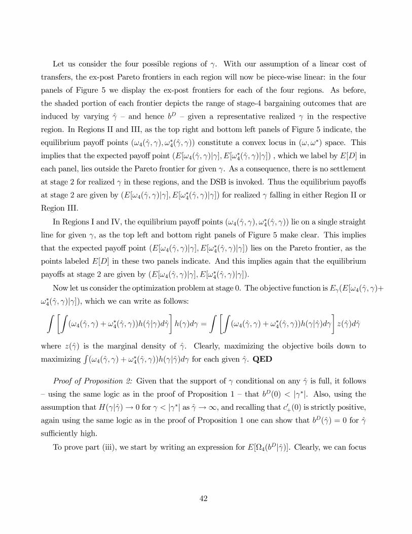
Let us consider the four possible regions of . With our assumption of a linear cost of
transfers, the ex-post Pareto frontiers in each region will now be piece-wise linear: in the four
panels of Figure 5 we display the ex-post frontiers for each of the four regions. As before,
the shaded portion of each frontier depicts the range of stage-4 bargaining outcomes that are
induced by varying — and hence — given a representative realized in the respective
region. In Regions II and III, as the top right and bottom left panels of Figure 5 indicate, the
equilibrium payoff points (4( ) ∗4( )) constitute a convex locus in (
∗) space. This
implies that the expected payoff point ([4( )|] [∗4( )|]) , which we label by [] ineach panel, lies outside the Pareto frontier for given . As a consequence, there is no settlement
at stage 2 for realized in these regions, and the DSB is invoked. Thus the equilibrium payoffs
at stage 2 are given by ([4( )|] [∗4( )|]) for realized falling in either Region II orRegion III.
In Regions I and IV, the equilibrium payoff points (4( ) ∗4( )) lie on a single straight
line for given , as the top left and bottom right panels of Figure 5 make clear. This implies
that the expected payoff point ([4( )|] [∗4( )|]) lies on the Pareto frontier, as thepoints labeled [] in these two panels indicate. And this implies again that the equilibrium
payoffs at stage 2 are given by ([4( )|] [∗4( )|])Now let us consider the optimization problem at stage 0. The objective function is([4( )+
∗4( )|]), which we can write as follows:Z ∙Z(4( ) + ∗4( ))(|)
¸() =
Z ∙Z(4( ) + ∗4( ))(|)
¸()
where () is the marginal density of . Clearly, maximizing the objective boils down to
maximizingR(4( ) + ∗4( ))(|) for each given . QED
Proof of Proposition 2: Given that the support of conditional on any is full, it follows
— using the same logic as in the proof of Proposition 1 — that (0) |∗|. Also, using theassumption that(|)→ 0 for |∗| as →∞, and recalling that 0+(0) is strictly positive,again using the same logic as in the proof of Proposition 1 one can show that () = 0 for
sufficiently high.
To prove part (iii), we start by writing an expression for [Ω4(|)]. Clearly, we can focus
42

on values of that are lower than |∗|, and hence we can write [Ω4(|)] as
Ω4(|) =
Z ()
0
( )(|) +Z ()
()
[ ( )− ( − |∗|)](|)
+
Z ∞
()
[ ( ) + + ∗ − ()](|)
Clearly [Ω4(|)] is differentiable in . Following similar steps as in the previous section,
and using the linear cost specification, we can write the first-order condition as:
[Ω4(|)]
= 0()(|∗|−)(()|)+
Z ()
()
(|)−Z ∞
()
(|) = 0 (7.3)
Note that the problem is smooth, hence the optimal is continuous in . Next we argue
that, if2 ln(|)
0, then 2Ω4
0 and hence the objective function is submodular in
and , which in turn implies that () is (weakly) decreasing. Notice that, for a given ,
the expression in (7.3) is a linear combination of density values (|) for different values of (noting that the integral of (|) is itself a linear combination). Noting that∆(()) 0 and 0() 0, it follows that the weights of this linear combination are positive for lower values
of (from () to ()) and negative for higher values of (from () to ∞). Therefore,if an increase in leads to a proportional change in (|) that is higher for higher values of, then the statement follows. But this is implied by the condition
2 ln(|)
0.
Finally we show that, if two random variables 1 and 2 are jointly normal with double
truncation at zero, then2 ln(2|1)
12 0. In this case, the conditional density of 2 given 1
takes the form (2|1) = · exp−(−)0Σ−1(−)∞0exp−(−)0Σ−1(−)2 , where = (1 2), is the mean of , Σ is
the covariance matrix of and is some constant. Note that the denominator is a function only
of 1, which we denote (1). Then we have ln(2|1)
1=
[−(−)0Σ−1(−)]1
− ln (1)
1, and hence
2 ln(2|1)12
=2[−(−)0Σ−1(−)]
12. Note that this is the same expression that would obtain with
a non-truncated normal distribution. The final step is to note that2[−(−)0Σ−1(−)]
12= −2,
where is the correlation parameter. Given that 0, the claim follows. QED
Proof of Proposition 4: It is easy to show that it cannot be optimal to set 0 or 0,
so we can focus on the case ≥ 0, ≤ 0. To keep the notation more intuitive we will thinkof the choice variables as being the absolute transfer levels, and | |.
43

We start by describing how the outcome of the stage-4 subgame varies with for given
levels of and | |. We need to consider separately two cases: + | | ≤ |∗| and + | | |∗|:
(a) If + | | ≤ |∗| :Again we can think of the importer as having two threat points: ( ) and ( | |); for
a generic value of , only one of the two threat points is active. For given and | |, thereare two critical levels of , (·) and (·), with (·) (·), such that: (I) for ∈ [0 (·)], the( | |) threat point is active, and there is no renegotiation, so the outcome is a policy of with the exporter paying | |; (II) for ∈ [(·) (·)], the ( ) threat point is active,but the DSB ruling is renegotiated and the equilibrium outcome is a policy of with the
exporter paying |∗| − ; and (III) for (·), the ( ) threat is active and there isno renegotiation, hence the outcome is a policy of with the importer paying . It is easy
to check that depends on both and | |, while depends only on , hence we write
( | |) and ()
(b) If + | | |∗| :In this case, the main change relative to the previous case is that (·) (·). As a
consequence, the equilibrium outcome is as follows: for ∈ [0 (·)], the ( | |) threat isactive, and there is no renegotiation, hence the outcome is a policy of with the exporter
paying | |; for ∈ [(·) (·)], the ( | |) threat is active, but there is renegotiation andthe equilibrium outcome is a policy of with the importer paying |∗|− | |; and for (·),the ( ) threat is active and there is no renegotiation, hence the outcome is a policy of
with the importer paying . We also note that in this case depends on both and | |,while depends only on | |.
It is not hard to argue that it can never be optimal to set + | | |∗|. Startingfrom a combination of and | | such that + | | |∗|, the objective function can beimproved weakly, for any given , by lowering to the level such that + | | = |∗|. Wewill therefore focus on the case + | | ≤ |∗| from here on.
As in the case considered in section 3.1, the equilibrium outcome of the stage-2 subgame
is the same as that of the stage-4 subgame. Moving back to stage 0, we need to consider how
the expected joint payoff depends on and | |. We let Ω( | |; ) denote the stage-2
44

joint payoff, and Ω( | |) its expectation with respect to , i.e. the stage-0 expected jointpayoff. Using a similar logic as the in the proof of Proposition 1, we can write the partial
derivatives Ω
and Ω| | :
Ω
= −0()(1−(()) + 0(|∗|− )[(())−(( | |))] (7.4)
+
(( | |))[( − |∗|)− (−| |)]
and
Ω
| | = 0(−| |)(( | |)) +
| |(( | |))[( − |∗|)− (−| |)] (7.5)
Note that
0, | | 0 and [(
− |∗|)− (−| |)] ≥ 0 (recall that + | | ≤ |∗|),so the last term of each equation is nonnegative. Also note that 0(−| |) 0.
We can now ask whether the optimal level of | | is zero or positive.Let us start with the case of full support, i.e. ∈ [0∞). A necessary condition for | | = 0
to be optimal is that the partial derivative Ω| | be non-positive when evaluated at | | = 0
and = , where is the optimal value of conditional on | | = 0. Recalling from
section 3.1 that ∈ (0 |∗|) when the support of is large enough, we can write¯Ω
| |
¯| |=0=
= −0+(0)(( 0)) +(·)| |((
0))( − |∗|)
The second term of this expression is strictly positive, and therefore we can conclude that, if
0+(0) is sufficiently small, the above expression is positive, and hence the optimal | | mustbe strictly positive.
Similarly, one can show that the optimal value of is strictly positive. Claim (ii) of
Proposition 4 follows.
We can now move to the case of small support of (around |∗|). Let us focus first on theknife-edge case = |∗|.Let us characterize how Ω( | |; |∗|) depends on and | |. Clearly, an optimum
requires that no transfer occur in equilibrium, and either policy or is optimal. Therefore
there are two sets of points ( | |) that are optimal: (i) any pair such that = 0 and
| | ∈ [0 |∗|] will induce the policy with zero transfer in equilibrium, and hence it is
45

optimal; (ii) any pair such that = 0 and ∈ [(|∗|) |∗|] will induce the policy
with zero transfer in equilibrium, and hence it is optimal.
For the analysis to follow, it is helpful to observe a few other properties of Ω( | |; |∗|):(1) For |∗|2, the ( ) threat is active and there is no renegotiation, hence the
equilibrium outcome is with the importer paying ;
(2) For |∗|2 −1(| | |∗|), the ( ) threat is active but there is renegotiation,and the equilibrium outcome is with the exporter paying |∗|−, where −1(| | ·) denotesthe inverse of (| | ·). We note that −1(| | |∗|) is decreasing in | | with slope between0 and -1, and satisfies −1(|∗|2 |∗|) = |∗|2 and −1(0 |∗|) = (|∗|);(3) For −1(| | |∗|), the ( | |) threat is active and there is no renegotiation,
hence the equilibrium outcome is with the exporter paying | |.Following a similar logic as in the proof of Proposition 1, we can ask what are the points
( | |) — other than the first-best points that we identified above — that yield a joint payoff“close to” the first best. The answer is: (a) those such that | | ∈ [0 |∗|] and 0 is close
to zero, and (b) those such that −1(| | |∗|) and | | 0 is close to zero. All otherpairs ( | |) yield a joint payoff that is discretely lower than the first best.We are now ready to consider a small support of around |∗|, say (|∗|−1 |∗|+2). Focus
first on pairs ( | |) of the type (a) described just above. For these pairs, Ω
0 for all
∈ (|∗|−1 |∗|+ 2), and hence no such pair can be optimal. Focus next on pairs ( | |)
of the type (b) described above; for these pairs, Ω| | 0 for all ∈ (|∗| − 1 |∗| + 2),
and hence no such pair can be optimal. All other pairs must be suboptimal too, because
by continuity they yield a joint payoff that is discretely lower than the first best for all ∈(|∗|− 1 |∗|+ 2), whereas we know that we can achieve a joint payoff close to the first best
with, for example,| | = 0 and (|∗|). Claim (i) of Proposition 4 follows directly.
QED
Proof of Proposition 5: Focus first on the first-order condition for , that is equation (7.4).
Applying the same logic as in section 3.2, it is easy to establish that, if2 ln(|)
0, then
2Ω
0 for any given | |. Next focus on the first-order condition for | |, that is equation(7.5): it is direct to verify that, if
2 ln(|)
0, then 2Ω| | 0 for any given . Using these
observations together with the assumption 2Ω| | 0, the claim follows directly. QED
46

References
Bagwell, Kyle and Robert W. Staiger (2005), “Enforcement, Private Political Pressure and
the GATT/WTO Escape Clause,” Journal of Legal Studies, June.
Bagwell, Kyle (2009), “Self-Enforcing Trade Agreements and Private Information,” unpub-
lished manuscript, Stanford University, February 15.
Baldwin, Richard, “Politically Realistic Objective Functions and Trade Policy,” Economics
Letters, vol. 24, pp. 287-90, 1987.
Beshkar, Mostafa (2008a),“Trade Skirmishes and Safeguards: A Theory of the WTO Dispute
Settlement Process,” unpublished manuscript, Purdue University, June.
Beshkar, Mostafa (2008b),“Optimal Remedies in International Trade Agreements,” unpub-
lished manuscript, Purdue University, May.
Grossman, Gene M. and Elhanan Helpman, “Protection for Sale,”American Economic Review,
84(4), pp. 833-850, 1994.
Hart, Henry and Albert Sacks (1958), The Legal Process: Basic Problems in the Making and
Application of Law (tent. ed.).
Hippler Bello, Judith (1996), “The WTO Dispute Settlement Understanding: Less is More,”
American Journal of International Law 90.
Hoekman, Bernard and Michel Kostecki (1995), The Political Economy of the World Trading
System, Oxford University Press, Oxford and New York.
Horn, Henrik and Petros C. Mavroidis (2008), “The WTO Dispute Settlement System 1995-
2006: Some Descriptive Statistics,” IFN Working Paper No. 740, Research Institute of
Industrial Economics.
Howse, Robert and Robert W. Staiger (2005), “United States—Anti-Dumping Act of 1916
(Original Complaint by the European Communities) — Recourse to arbitration by the
47

United States under 22.6 of the DSU, WT/DS136/ARB, 24 February 2004: A legal and
Economic Analysis,” World Trade Review 4:2, 295-316.
Jackson, John H. (1997), “The WTO Dispute Settlement Understanding—Misunderstandings
on the Nature of Legal Obligation,” The American Journal of International Law 91 (1),
January, pp. 60-64.
Kaplow, Louis and Steven Shavell (1996), “Property Rules versus Liability Rules: An Eco-
nomic Analysis,” Harvard Law Review 109 (4), pp. 713-790
Maggi, Giovanni and Robert W. Staiger (2008), “The Role of Dispute Settlement Procedures
in International Trade Agreements,” NBER Working Paper No. 14067, June.
Martin, Alberto and Wouter Vergote (2008), “On the Role of Retaliation in Trade Agree-
ments,” Journal of International Economics 76(1).
Mnookin, Robert H. and Lewis Kornhauser (1979), “Bargaining in the Shadow of the Law:
the Case of Divorce,” 88 Yale Law Journal 950.
Park, Jee-Hyeong (2009), “Enforcing International Trade Agreements with Imperfect Private
Monitoring: Private Trigger Strategies and a Possible Role for the WTO,” unpublished
manuscript, Seoul National University, February.
Schwartz, Alan (1979), “The Case for Specific Performance,” Yale Law Journal 89.
Schwartz, Warren F. and Alan O. Sykes (2002), “The Economic Structure of Renegotiation
and Dispute Resolution in the World Trade Organization,” Journal of Legal Studies 31.
Shavell, Steven (2006), “Specific Performance versus Damages for Breach of Contract: An
Economic Analysis,” Texas Law Review 84, March.
Ulen, Thomas S. (1984), “The Efficiency of Specific Performance: Toward a Unified Theory
of Contract Remedy,” Michigan Law Review 83.
USTR (2001), “U.S. Trade Representative Announces the Lifting of Sanctions on European
Products as EU Opens Market to U.S. Banana Distributors,” Press Release, July 1.
48

Figure 1
ω*
ω
slope = -1
Pareto Frontier for Region III
FT
P
0
| γ*|
γ
ω*
ω
slope = -1
Pareto Frontier for Region IV
FT
P
0
| γ*|
γ
ω*
ω
slope = -1
Pareto Frontier for Region I
FT
P
0
| γ*|
γ
ω*
ω
slope = -1
Pareto Frontier for Region II
FT
P
0
| γ*|
γ

Figure 2
ω*
ω
slope = -1
Bargaining Outcome in Light of Damages bD: Region II
FT
P
0
R
J
bD
b
| γ*|
γ
bD
Ω
Joint Welfare (Ω) and Damages (bD): Region II
ΩFB
ΩFB + Γ
0 breneg bprohib | γ*|
ω*
ω
slope = -1
Bargaining Outcome in Light of Damages bD: Region III
FT
P
0
R
J
bD
b
| γ*|
γ
bD
Ω
Joint Welfare (Ω) and Damages (bD): Region III
ΩFB
ΩFB - Γ
0 breneg bprohib | γ*|

Figure 3
ω*
ω
slope = -1
Bargaining Outcome in Light of Damages bD: Region II/III Border
FT
P
0
R
JbD
b
γ
| γ*|
bD
Ω
Joint Welfare (Ω) and Damages (bD): Border of Regions II/III
ΩFB
0 breneg bprohib | γ*|

Figure 4
ω*
ω
slope = -1
Bargaining Outcome in Light of Damages bD: Region I
FT
P
0
J
bD
b
| γ*|
γ
bD
Ω
Joint Welfare (Ω) and Damages (bD): Region I
bprohib
ΩFB
ΩFB + Γ
0 | γ*|
ω*
ω
slope = -1
Bargaining Outcome in Light of Damages bD: Region IV
FT
P
0
J
bD
b
| γ*|
γ
bD
Ω
Joint Welfare (Ω) and Damages (bD): Region IV
ΩFB
ΩFB - Γ
0 bprohib| γ*|

Figure 5
ω*
ω
Bargaining Outcome in Light of Uncertain Damages: Region I
FT
0
E[D]
ω*
ω
Bargaining Outcome in Light of Uncertain Damages: Region II
FT
P
0
E[D]
ω*
ω
Bargaining Outcome in Light of Uncertain Damages: Region III
FT
P
0
E[D]
ω*
ωBargaining Outcome in Light of Uncertain Damages: Region IV
P
0
E[D]
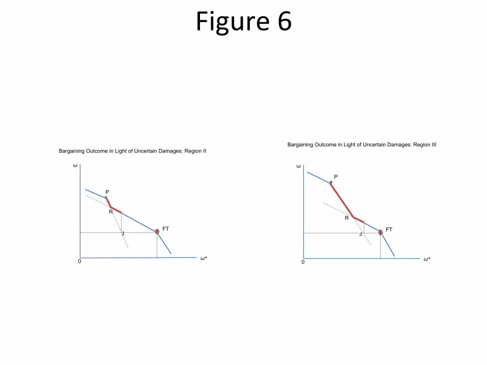
Figure 6
ω*
ω
Bargaining Outcome in Light of Uncertain Damages: Region III
FT
P
0
R
J
ω*
ω
Bargaining Outcome in Light of Uncertain Damages: Region II
FT
P
0
R
J