BPS - 5th Ed. Chapter 171 Inference about a Population Mean.

BPS - 5th Ed. Chapter 17 1

Chapter 17

Inference about a Population Mean


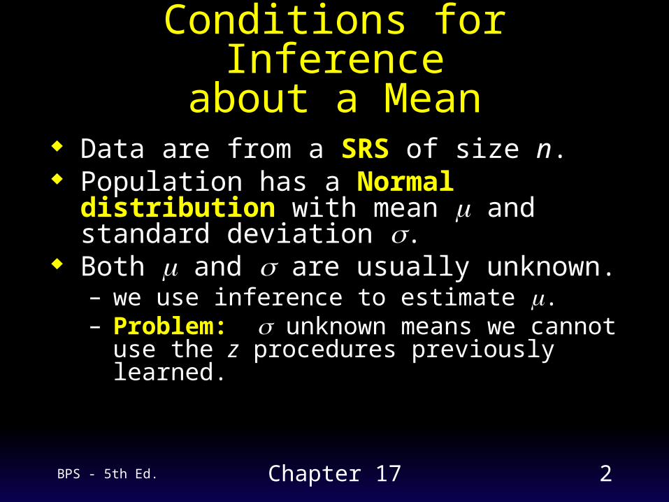
Conditions for Inferenceabout a Mean

Data are from a SRS of size n. Population has a Normal distribution

with mean and standard deviation . Both and are usually unknown.

– we use inference to estimate .– Problem: unknown means we cannot

use the z procedures previously learned.


When we do not know the population standard deviation (which is usually the case), we must estimate it with the sample standard deviation s.

When the standard deviation of a statistic is estimated from data, the result is called the standard error of the statistic.

The standard error of the sample mean is

Standard Error

x

sn


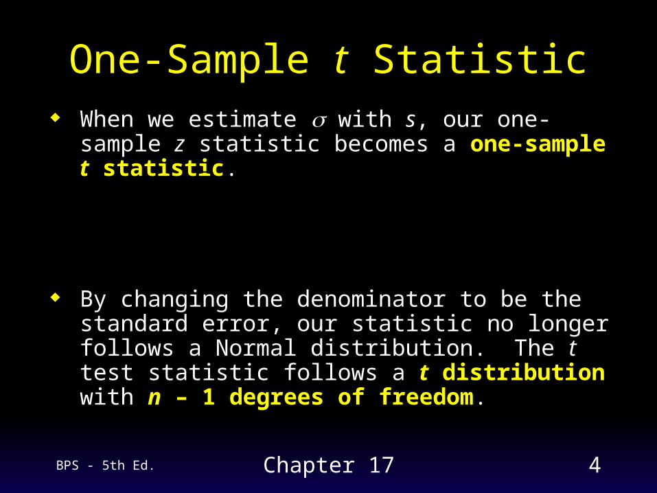
When we estimate with s, our one-sample z statistic becomes a one-sample t statistic.

By changing the denominator to be the standard error, our statistic no longer follows a Normal distribution. The t test statistic follows a t distribution with n – 1 degrees of freedom.

One-Sample t Statistic

ns

μxt

nσ

μxz 00


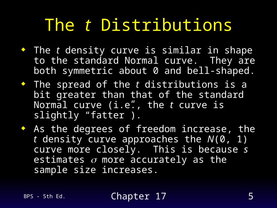
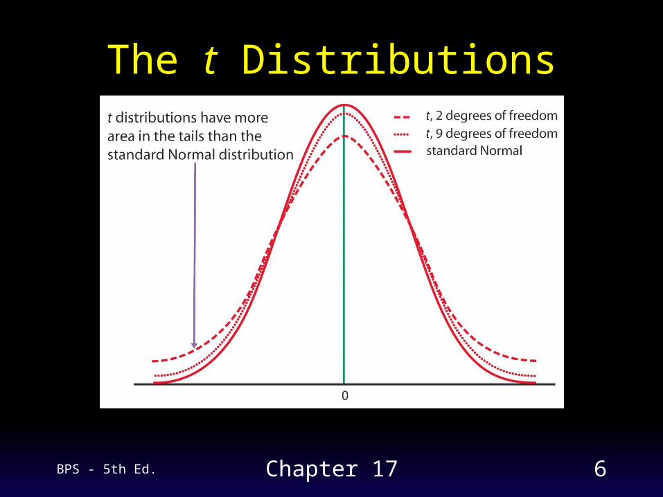
The t Distributions The t density curve is similar in shape to the

standard Normal curve. They are both symmetric about 0 and bell-shaped.

The spread of the t distributions is a bit greater than that of the standard Normal curve (i.e., the t curve is slightly “fatter”).

As the degrees of freedom increase, the t density curve approaches the N(0, 1) curve more closely. This is because s estimates more accurately as the sample size increases.


The t Distributions


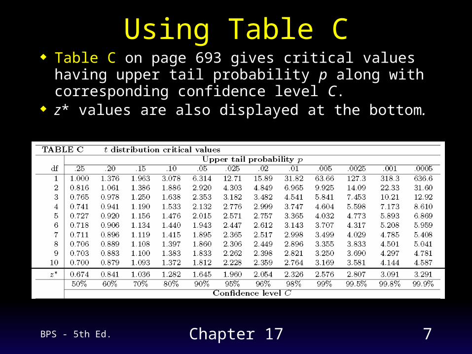
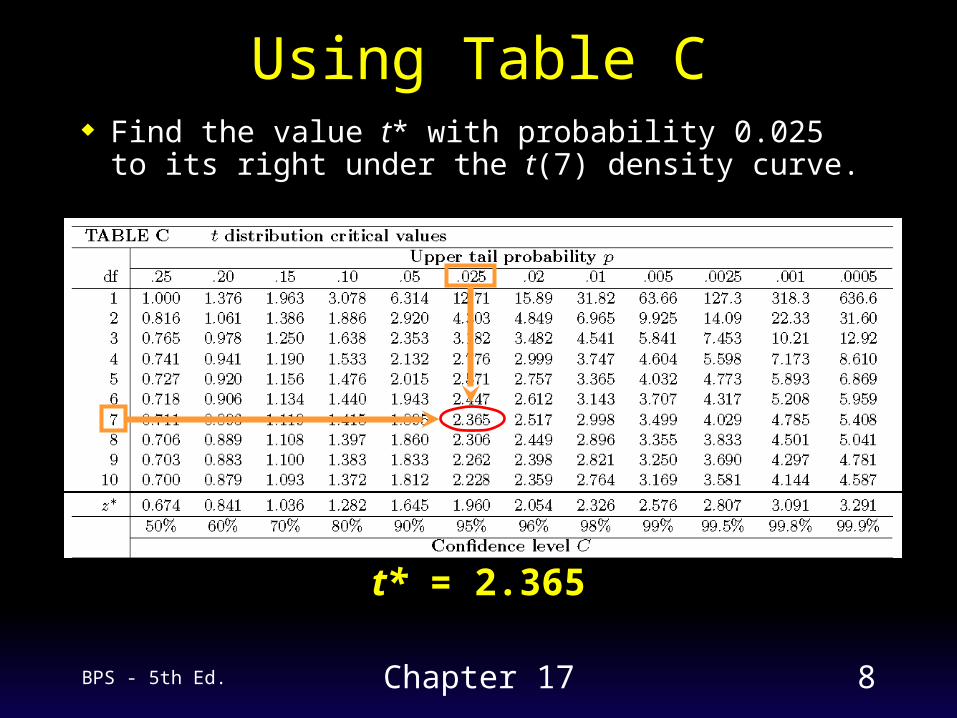
Using Table C Table C on page 693 gives critical values

having upper tail probability p along with corresponding confidence level C.

z* values are also displayed at the bottom.


Using Table C Find the value t* with probability 0.025 to its

right under the t(7) density curve.

t* = 2.365


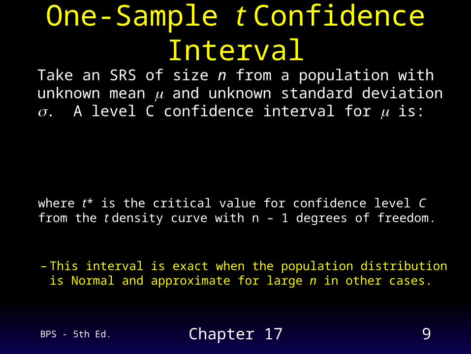
– This interval is exact when the population distribution is Normal and approximate for large n in other cases.

where t* is the critical value for confidence level C from the t density curve with n – 1 degrees of freedom.

Take an SRS of size n from a population with unknown mean and unknown standard deviation . A level C confidence interval for is:

One-Sample t Confidence Interval

nstx


Case StudyAmerican Adult Heights

70.686 to 63.714

3.48667.27

3.92.36567.2

n

stx

A study of 7 American adults from an SRS yields an average height of = 67.2 inches and a standard deviation of s = 3.9 inches. A 95% confidence interval for the average height of all American adults () is:

x

“We are 95% confident that the average height of all American adults is between 63.714 and 70.686 inches.”


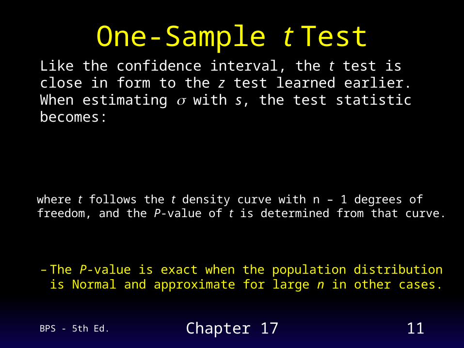
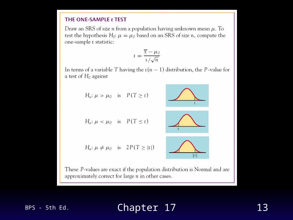
– The P-value is exact when the population distribution is Normal and approximate for large n in other cases.

where t follows the t density curve with n – 1 degrees of freedom, and the P-value of t is determined from that curve.

Like the confidence interval, the t test is close in form to the z test learned earlier. When estimating with s, the test statistic becomes:

One-Sample t Test

ns

μxt 0


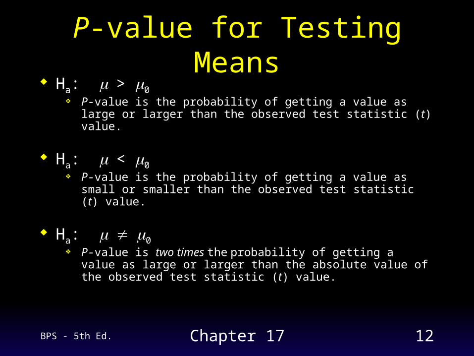
P-value for Testing Means Ha: > 0

P-value is the probability of getting a value as large or larger than the observed test statistic (t) value.

Ha: < 0 P-value is the probability of getting a value as small or

smaller than the observed test statistic (t) value.

Ha: 0 P-value is two times the probability of getting a value as

large or larger than the absolute value of the observed test statistic (t) value.


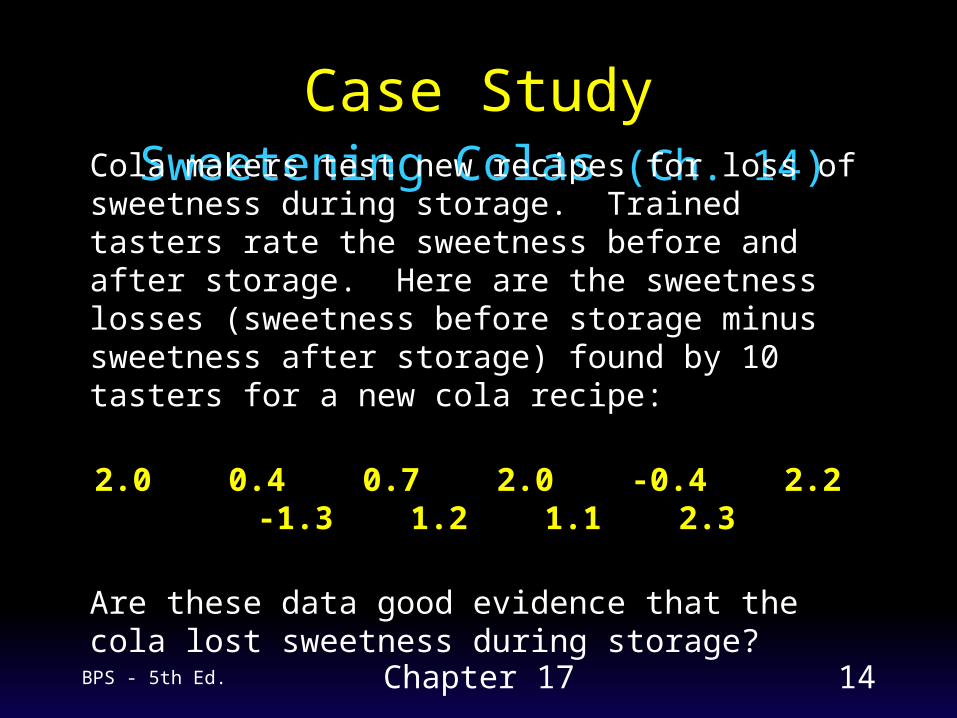
Sweetening Colas (Ch. 14)

Case Study

Cola makers test new recipes for loss of sweetness during storage. Trained tasters rate the sweetness before and after storage. Here are the sweetness losses (sweetness before storage minus sweetness after storage) found by 10 tasters for a new cola recipe:

2.0 0.4 0.7 2.0 -0.4 2.2 -1.3 1.2 1.1 2.3

Are these data good evidence that the cola lost sweetness during storage?


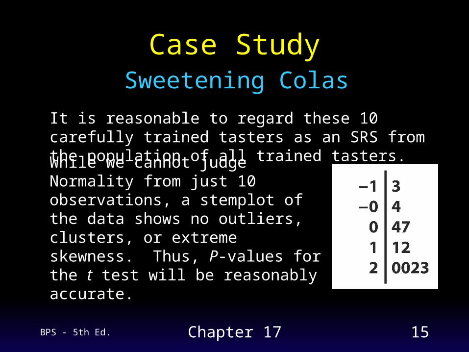
Case Study

It is reasonable to regard these 10 carefully trained tasters as an SRS from the population of all trained tasters.

While we cannot judge Normality from just 10 observations, a stemplot of the data shows no outliers, clusters, or extreme skewness. Thus, P-values for the t test will be reasonably accurate.

Sweetening Colas


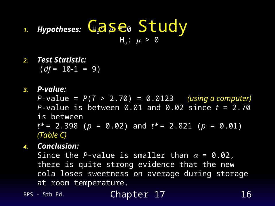
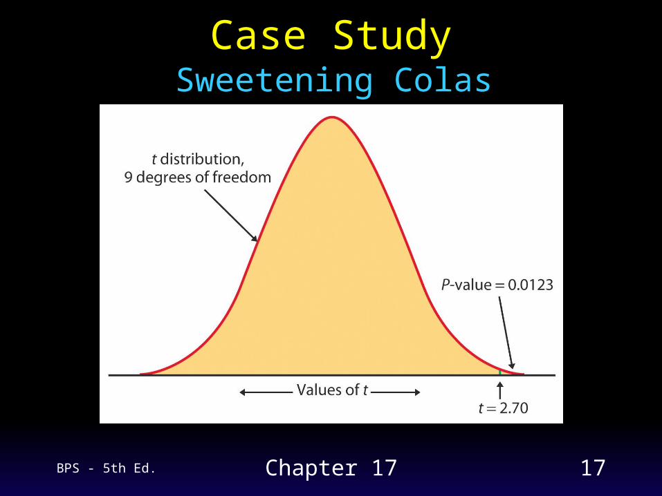
1. Hypotheses: H0: = 0Ha: > 0

2. Test Statistic: (df = 101 = 9)

3. P-value:P-value = P(T > 2.70) = 0.0123 (using a computer)P-value is between 0.01 and 0.02 since t = 2.70 is between t* = 2.398 (p = 0.02) and t* = 2.821 (p = 0.01) (Table C)

4. Conclusion:Since the P-value is smaller than = 0.02, there is quite strong evidence that the new cola loses sweetness on average during storage at room temperature.

2.70

101.196

01.020

ns

μxt

Case Study


Sweetening ColasCase Study


Matched Pairs t Procedures To compare two treatments, subjects are matched in

pairs and each treatment is given to one subject in each pair.

Before-and-after observations on the same subjects also calls for using matched pairs.

To compare the responses to the two treatments in a matched pairs design, apply the one-sample t procedures to the observed differences (one treatment observation minus the other).

The parameter is the mean difference in the responses to the two treatments within matched pairs of subjects in the entire population.


Air Pollution

Case Study

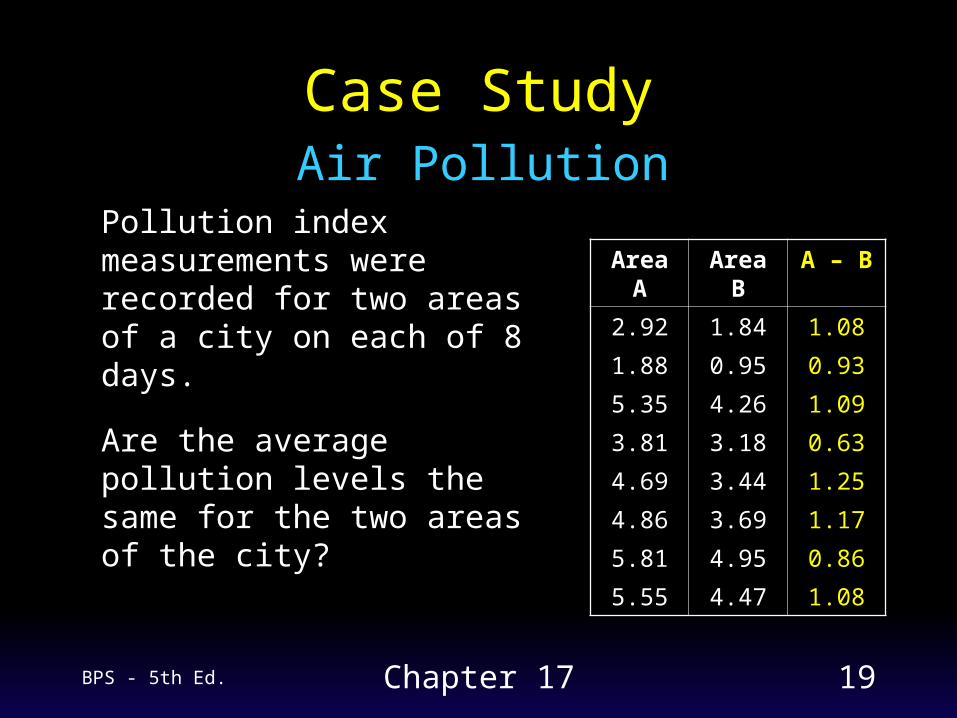
Pollution index measurements were recorded for two areas of a city on each of 8 days.

Are the average pollution levels the same for the two areas of the city?

Area A Area B A – B

2.92 1.84 1.08

1.88 0.95 0.93

5.35 4.26 1.09

3.81 3.18 0.63

4.69 3.44 1.25

4.86 3.69 1.17

5.81 4.95 0.86

5.55 4.47 1.08


Air Pollution

Case Study

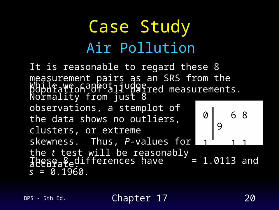
It is reasonable to regard these 8 measurement pairs as an SRS from the population of all paired measurements.

While we cannot judge Normality from just 8 observations, a stemplot of the data shows no outliers, clusters, or extreme skewness. Thus, P-values for the t test will be reasonably accurate.

0 6 8 9

1 1 1 1 2 2

These 8 differences have = 1.0113 and s = 0.1960.

x


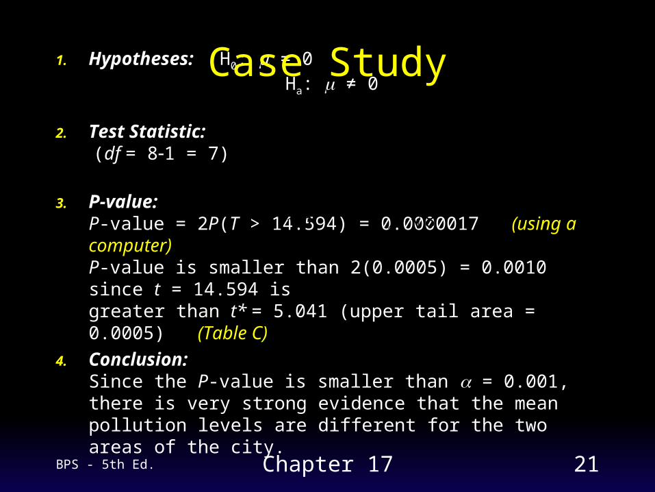
1. Hypotheses: H0: = 0Ha: ≠ 0

2. Test Statistic: (df = 81 = 7)

3. P-value:P-value = 2P(T > 14.594) = 0.0000017 (using a computer)P-value is smaller than 2(0.0005) = 0.0010 since t = 14.594 is greater than t* = 5.041 (upper tail area = 0.0005) (Table C)

4. Conclusion:Since the P-value is smaller than = 0.001, there is very strong evidence that the mean pollution levels are different for the two areas of the city.

14.594

80.1960

01.01130

ns

μxt

Case Study


1.1752 to 0.8474

0.16391.01138

0.19602.3651.0113

n

stx

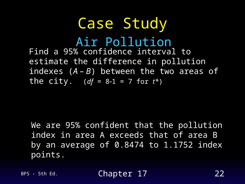
Find a 95% confidence interval to estimate the difference in pollution indexes (A – B) between the two areas of the city. (df = 81 = 7 for t*)

We are 95% confident that the pollution index in area A exceeds that of area B by an average of 0.8474 to 1.1752 index points.

Case StudyAir Pollution


Robustness of t Procedures The t confidence interval and test are exactly

correct when the distribution of the population is exactly normal.

No real data are exactly Normal. The usefulness of the t procedures in practice

therefore depends on how strongly they are affected by lack of Normality.

A confidence interval or significance test is called robust if the confidence level or P-value does not change very much when the conditions for use of the procedure are violated.


Using the t Procedures Except in the case of small samples, the assumption that

the data are an SRS from the population of interest is more important than the assumption that the population distribution is Normal.

Sample size less than 15: Use t procedures if the data appear close to Normal (symmetric, single peak, no outliers). If the data are skewed or if outliers are present, do not use t.

Sample size at least 15: The t procedures can be used except in the presence of outliers or strong skewness in the data.

Large samples: The t procedures can be used even for clearly skewed distributions when the sample is large, roughly n ≥ 40.


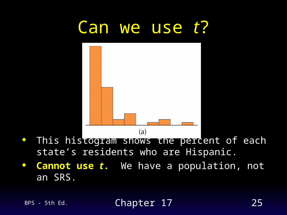
Can we use t?

This histogram shows the percent of each state’s residents who are Hispanic.

Cannot use t. We have a population, not an SRS.


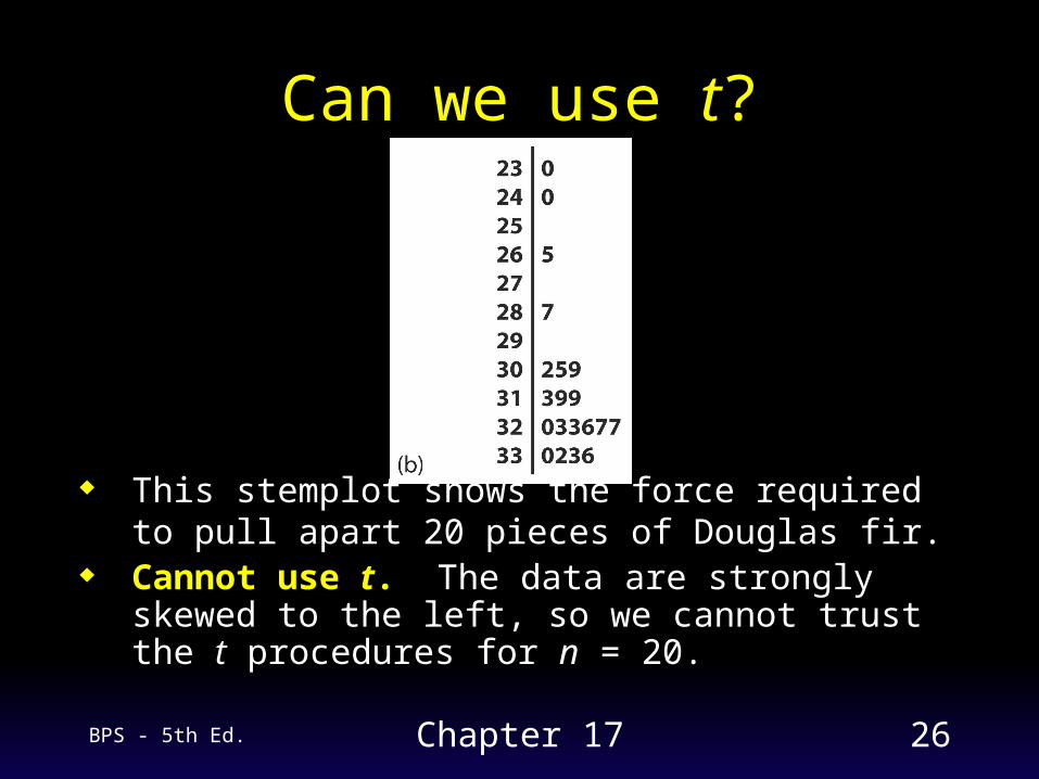
Can we use t?

This stemplot shows the force required to pull apart 20 pieces of Douglas fir.

Cannot use t. The data are strongly skewed to the left, so we cannot trust the t procedures for n = 20.


Can we use t?

This histogram shows the distribution of word lengths in Shakespeare’s plays.

Can use t. The data is skewed right, but there are no outliers. We can use the t procedures since n ≥ 40.


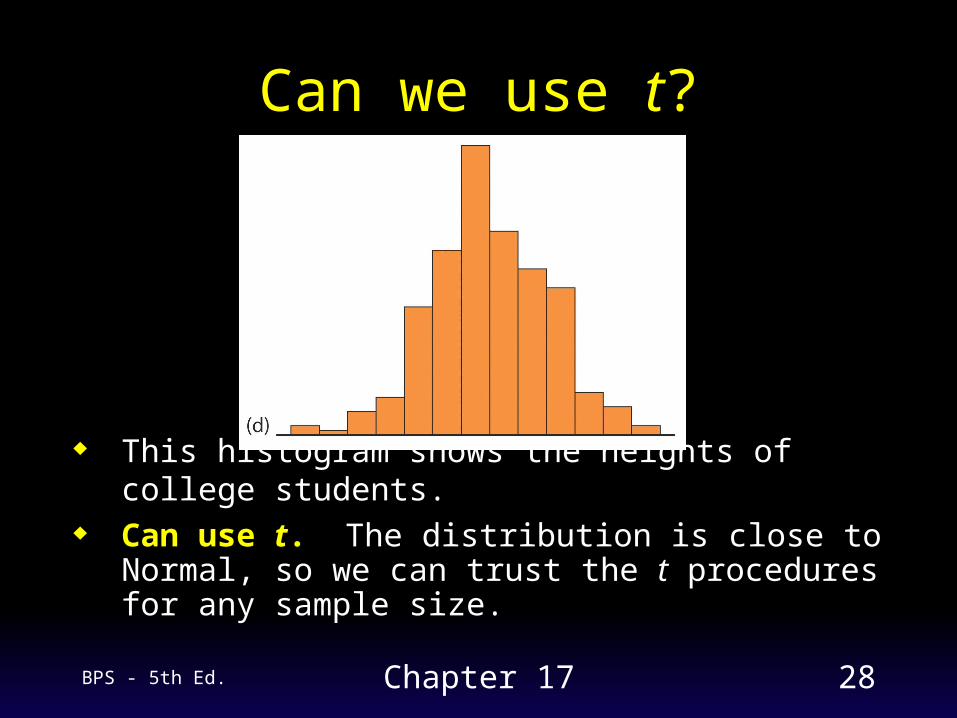
Can we use t?

This histogram shows the heights of college students. Can use t. The distribution is close to Normal, so we

can trust the t procedures for any sample size.

BPS - 5th Ed. Chapter 171 Inference about a Population Mean.

Documents

Transcript of BPS - 5th Ed. Chapter 171 Inference about a Population Mean.