Boys Lag Behind: How Teachers' Gender Biases Affect ...ftp.iza.org/dp10343.pdf · Boys Lag Behind:...
61
Forschungsinstitut zur Zukunft der Arbeit Institute for the Study of Labor DISCUSSION PAPER SERIES Boys Lag Behind: How Teachers’ Gender Biases Affect Student Achievement IZA DP No. 10343 November 2016 Camille Terrier
Transcript of Boys Lag Behind: How Teachers' Gender Biases Affect ...ftp.iza.org/dp10343.pdf · Boys Lag Behind:...

Forschungsinstitut zur Zukunft der ArbeitInstitute for the Study of Labor
DI
SC
US
SI
ON
P
AP
ER
S
ER
IE
S
Boys Lag Behind: How Teachers’ Gender Biases Affect Student Achievement
IZA DP No. 10343
November 2016
Camille Terrier
Boys Lag Behind:
How Teachers’ Gender Biases Affect Student Achievement
Camille Terrier MIT, IZA and CEP
Discussion Paper No. 10343 November 2016
IZA
P.O. Box 7240 53072 Bonn
Germany
Phone: +49-228-3894-0 Fax: +49-228-3894-180
E-mail: [email protected]
Any opinions expressed here are those of the author(s) and not those of IZA. Research published in this series may include views on policy, but the institute itself takes no institutional policy positions. The IZA research network is committed to the IZA Guiding Principles of Research Integrity. The Institute for the Study of Labor (IZA) in Bonn is a local and virtual international research center and a place of communication between science, politics and business. IZA is an independent nonprofit organization supported by Deutsche Post Foundation. The center is associated with the University of Bonn and offers a stimulating research environment through its international network, workshops and conferences, data service, project support, research visits and doctoral program. IZA engages in (i) original and internationally competitive research in all fields of labor economics, (ii) development of policy concepts, and (iii) dissemination of research results and concepts to the interested public. IZA Discussion Papers often represent preliminary work and are circulated to encourage discussion. Citation of such a paper should account for its provisional character. A revised version may be available directly from the author.

IZA Discussion Paper No. 10343 November 2016
ABSTRACT
Boys Lag Behind: How Teachers’ Gender Biases Affect Student Achievement* I use a combination of blind and non-blind test scores to show that middle school teachers favor girls when they grade. This favoritism, estimated in the form of individual teacher effects, has long-term consequences: as measured by their national evaluations three years later, male students make less progress than their female counterparts. Gender-biased grading accounts for 21 percent of boys falling behind girls in math during middle school. On the other hand, girls who benefit from gender bias in math are more likely to select a science track in high school. JEL Classification: I21, I24, J16 Keywords: teachers, gender biases, progress, achievement inequalities Corresponding author: Camille Terrier Department of Economics Massachusetts Institute of Technology 50 Memorial Dr. Cambridge, MA 02142 USA E-mail: [email protected]
* I would especially like to thank my advisor, Marc Gurgand. This paper also benefited from discussions with and helpful comments from Joshua Angrist, David Autor, Esteban Aucejo, Elizabeth Beasley, Thomas Breda, Ricardo Estrada, Victor Lavy, Alan Manning, Eric Maurin, Stephen Machin, Sandra McNally, Steve Pischke, Corinne Prost, and anonymous referees and participants at various seminars and conferences. I am especially grateful to Francesco Avvisati, Marc Gurgand, Nina Guyon, and Eric Maurin for sharing their dataset, as well as to the Direction de l’Evaluation, de la Prospective et de la Performance (DEPP) of the French Ministry of Education for giving me access to complementary data used in this paper. A previous version of this paper circulated as a CEP Discussion Paper no. 1341 - March 2015.
Boys are increasingly lagging behind girls at school.1 This disadvantage has important
consequences: boys who fall behind are at risk of dropping out of school, not attending college
or university, and/or being unemployed. In OECD countries, 66 percent of women entered
a university program in 2009, versus 52 percent of men, and this gap is increasing (OECD
(2012)). In Europe, 43 percent of women aged 30–34 completed tertiary education in 2015,
compared to 34 percent of men in the same age range. Because this gap has increased by
4.4 percentage points in the last ten years, there is a growing interest in identifying its roots.2
Some recent studies have highlighted the role of school-related inputs, such as school quality
(Autor et al. (2016)), peer socio-economic status (Legewie, DiPrete (2012)), teacher gender
(Dee (2005)), or teaching focus on literacy or numeracy (Machin, McNally (2005)).
This article complements this literature by demonstrating how teachers’ gender biases affect
their pupils’ progress and schooling decisions. A number of papers have shown that stereo-
typing can bias teachers’ assessment and grades, but the impact of such biases has yet to be
addressed.3 Prior research on that topic is limited, and it has focused on specific mechanisms
through which a gender bias could affect progress. Research shows that teachers’ biases gen-
erate self-fulfilling prophecies (Jussim, Eccles (1992)), produce stereotype threats4 (Steele,
Aronson (1995), Spencer et al. (1999), Hoff, Pandey (2006)), affect students’ interest in a sub-
ject (Marsh, Craven (1997), Trautwein et al. (2006), Bonesrønning (2008)), and affect students’
levels of effort5 (Mechtenberg (2009)). To my knowledge, this is one of the first papers to pro-
1In OECD countries, "15-year-old boys are more likely than girls, on average, to fail to attain a baseline levelof proficiency in reading, mathematics and science” (OECD (2015)).
2In France, 49.6 percent of women aged 30–34 have completed tertiary education in 2015, compared to only40.3 percent of their male counterparts.
3See for instance Bar, Zussman (2012), Burgess, Greaves (2013), Hanna, Linden (2012) on teachers’ genderbias, and Tiedemann (2000) and Fennema et al. (1990) for the existence of a gender bias in mathematics. Severalpapers have exploited blind and non-blind scores (teachers’ grades) to test the existence of such biases in teachers’grades, a methodology introduced in a seminal paper by Lavy (2008). Some papers find that girls benefit fromgrade discrimination (Lindahl (2007), Lavy (2008), Robinson, Lubienski (2011), Falch, Naper (2013), Cornwellet al. (2013)), while others find no gender bias (Hinnerich et al. (2011)). Ouazad, Page (2013) and Dee (2007)observed that gender biases depend on teachers’ genders. Breda, Ly (2015) found that discrimination depends onthe degree to which the subject is “male-connoted”.
4The latter arises when girls or minority groups perform poorly for the sole reason that they fear confirming thestereotype that their group performs poorly. The apprehension it causes might disrupt women’s math performance.Therefore, over-grading girls can reduce their anxiety to be judged as poor performers when they undergo a mathexam.
5Mechtenberg (2009) provided a theoretical model of how biased grading at school can explain gender differ-ences in achievements. School results are defined as a combination of talent and effort, the latter being the channel
1

vide empirical evidence on how teachers’ gender biases affect pupils’ progress and schooling
decisions, along with a contemporaneous and independent study by Lavy, Sand (2015).6
I use a rich student-level dataset produced by Avvisati et al. (2014) that follows 4490 pupils
from grade 6. To quantify teachers’ gender biases in math and literacy, I exploit an essential
feature of the data: it contains both blind and non-blind scores. An external corrector without
knowledge of student’s characteristics provides schools with blind scores. These scores are
therefore presumably free of teachers’ biases. Teachers provide the non-blind scores at the
same period for in-class exams. Both scores are designed to measure the same skills—an
assumption that I discuss and test in the paper.7 In addition, the data allows us to follow pupils
over time. The dataset contains blind scores up to grade 9, the high schools attended by each
student (general, professional, or technical), and students’ course choices during high school
(scientific, literature, or social sciences). This gives me the opportunity to study the long-term
impact of teachers’ gender biases on pupils’ progress, schools attended, and course choices.
I start by documenting extensive gender bias in teacher evaluations in grade 6. Follow-
ing the footsteps of many previous studies, I use a double-difference (DiD) methodology to
measure teachers’ gender biases (Falch, Naper (2013), Breda, Ly (2015), Lavy (2008), Goldin,
Rouse (2000), and Blank (1991)). The gender bias is defined as the average gap between non-
blind and blind scores for girls, minus this same gap for boys.8 Overall, I find a substantial
bias against boys in math, representing 0.3 points of the standard deviation (SD). This tends
to confirm existing studies that find that girls are favored by teachers in math (Falch, Naper
(2013), Breda, Ly (2015)). However, no gender bias is observed in literacy. Taking boys’ more
disruptive behavior and students’ initial achievement into account does not affect the estimate
through which gender grade biases could affect future cognitive achievement.6Lavy, Sand (2015) analyze a similar question, using the conditional random assignment of pupils to classes
and the differences in teachers’ stereotypical attitudes to identify the effect that teachers’ gender biases have onboys’ and girls’ respective progress.
7This dataset also contains extensive information on pupils’ disruptive behavior in the classroom, which allowsme to disentangle a bias related to gender from a bias related to pupils’ behavior.
8This double difference can be interpreted as a gender bias in teachers’ grades if the blind and non-blind scoresmeasure exactly the same skills. However, if the grades given by teachers measure slightly different skills (home-work for instance), for which boys or girls have an advantage, then the double difference should be interpretedmore broadly as a bias in teachers’ evaluation methods. The correlation between abilities tested by both scores istested in the paper, and happens to be equal to 1.
2
significantly. Compared to the existing literature that uses this DiD method to measure an
average gender bias, I will exploit the variation of the gender bias between teachers.
To identify the impact of teachers’ gender biases on pupils’ progress, I use a novel identifi-
cation strategy that rests on both the variation in teachers’ gender biases and the quasi-random
assignment of students to biased teachers. The identification therefore stems from a compari-
son of the relative progress of girls (as compared to boys) in classes where the teacher displays
a high degree of bias to the relative progress of girls in classes where the teacher is not very
biased. I use a simple latent variable model of a student’s progress to recover the reduced-form
regression. This model aims to highlight the potential sources of endogeneity that could pre-
vent identification. It disentangles the effect of teachers’ gender biases on a student’s progress
from three other elements that might be correlated to both a teacher’s gender bias and students’
progress: a pupil’s achievement, boys’ or girls’ unobserved characteristics, and teacher quality.
It is key for the identification that the students are quasi-randomly assigned to the teachers
with different degrees of bias. I check that students’ gender, social background, initial achieve-
ment, and grade repetition are uncorrelated to the gender bias of the teachers. I also show that
the gender bias I measure with the double-differences methodology does not capture students’
unobserved characteristics–such as stress, response to the stakes of the exams, and the compet-
itiveness of the environment–that might be correlated to progress. In addition, to ensure that
I disentangle the impact of a teacher’s quality from the effect of his/her gender bias, I use a
first-difference specification (between boys and girls) that cancels the teacher’s effects. Finally,
because a gender bias is estimated for each teacher, the number of observations for each es-
timation is limited. The resulting estimation error would lead to attenuation bias when I use
the teacher bias measure in regressions as an explanatory variable for students’ progress. To
address the sampling error, I use empirical Bayes estimates of teacher gender biases (Kane,
Staiger (2002)).
The main finding is that teachers’ gender biases have a high and significant effect on boys’
progress relative to girls in both math and literacy.9 For two classes where the achievement
9In interpreting the results, I show that my analysis identifies three effects that I cannot completely disentangle:(1) teachers’ gender bias in grades, (2) teachers’ potentially biased evaluation methods (for instance, some teachers
3

gap between boys and girls would be identical in 6th grade, quasi-randomly assigning a teacher
who is 1 SD more biased against boys in one of the classes decreases boys’ progress in that
class relative to girls by 0.136 SD in math and by 0.129 SD in literacy. Over the four years of
middle school, teachers’ gender bias against boys accounts for 21 percent of boys falling behind
girls in math. Then, analyzing the effect separately for boys and girls, I find that having a math
teacher who is 1 SD more biased against boys does not impact boys’ progress, but significantly
increases girls’ progress. Conversely, a biased literacy teacher does not impact girls’ progress,
but significantly reduces boys’ progress. This interesting difference might be related to gender
differences in self-confidence, which could differ by subject.
Moving to outcomes during high school (four years after the bias), I find that having a
math teacher who is 1 SD more biased in favor of girls increases girls’ probability of selecting
a scientific track in high school by 2.7 percentage points compared to boys. Interestingly,
without teachers’ bias in favor of girls, the gender gap in choosing a science track–a predictor
of careers in STEM fields–would be 11.7 percent larger in favor of boys. On the other hand,
teachers’ gender biases do not impact boys’ relative probability to attend a general high school
(rather than a professional or technical one) or to repeat a grade. I am also able to rule out some
potential mechanisms. Teachers’ biases do not have a cumulative effect: being reassigned to
the same biased teacher for a second consecutive year does not further impede boys’ relative
progress. Similarly, teachers’ gender biases have no spillover effect: a bias in a given subject
does not impact boys’ relative progress in other subjects. Finally, as robustness checks, I show
that the blind and non-blind scores measure abilities that are very similar and that the time lag
between both scores creates an attenuation bias on my estimates.
Taken together, these results build upon an important literature that suggests teachers’
grades are biased. My findings confirm the existence of such biases, but more importantly, they
highlight the fact that teachers’ gender biases can have long-lasting effects on boys and girls’
human capital accumulation, and therefore on the evolution of gender inequalities at school and
might use more homework as an evaluation tool, and boys and girls might perform differently at homework), and(3) teachers’ behavior in class, which might favor girls or boys. I try to disentangle the latter effect by measuringstudents’ progress over a period where they do not interact with the biased teacher.
4

in the labor market. From an academic perspective, this article contributes to the recent and
growing literature on the impact of teachers’ discretion in grading on students’ success (Apper-
son et al. (2016), Dee et al. (2016), and Diamond, Persson (2016)). This paper also contributes,
though indirectly, to the literature highlighting the importance of students’ non-cognitive skills
(Heckman, Rubinstein (2001)). Previous work has focused on the effect of parental inputs on
students’ non-cognitive skills (Cunha, Heckman (2008)), while this paper focuses on teachers
as another potentially key input.
I Data
I.A Dataset
I consider the question of teachers’ assessment biases by using a French dataset that covers
35 middle schools, 191 classes, and 4490 pupils. All students are first observed during grade
6 (11 years old), the first year of middle school. Blind and non-blind scores are available
for each student. Students obtain the blind score when they complete a standardized test at
the beginning and end of grade 6. The French Education Ministry created this test, taken
annually by all French pupils, to assess students’ cognitive skills. Identical across all schools,
it tests knowledge on literacy (reading and writing) and mathematics. Importantly, this test is
externally graded, and graders do not know the names, genders, social backgrounds, or behavior
of pupils they evaluate. This blind score can therefore be assumed to be free of any bias caused
by stereotypes from an external examiner. Each student also receives grades from teachers on
in-class exams. A pupil has a different teacher in each subject, and each teacher reports their
pupils’ average grades on end-of-term report cards. In this study, I use information on the
average grade given by teachers in math and literacy during the first and last terms of grade
6. Because teachers have permanent contact with the pupils they teach, these average grades
could potentially be biased by teachers’ gender stereotypes.
The standardized test and class exams are designed to measure the same abilities. Appendix
A.1 describes abilities measured respectively by the blind and the non-blind scores. Both tests
5

are also taken under the same conditions: pupils fill in both tests in their usual classrooms, and
their teachers give instructions. Blind and non-blind tests also include questions with different
degrees of difficulty. The national evaluation relies heavily on written questions: in literacy,
only 18 percent of questions are multiple choice, with the remaining 82 percent requiring writ-
ten answers. The percentage is even higher in math, where 95 percent of the questions require
written answers. The reliance on written questions makes the national evaluation format simi-
lar to in-class exams, where multiple-choice questions are quite rare.10 This similarity is partly
due to grade 6 teachers: 49 percent of literacy teachers and 47 percent of math teachers report
using the standardized evaluation provided by the ministry as a benchmark to create their own
class exams (French Ministry of Education (2005)). However, despite featuring similar types
of questions, the formats of both tests might differ. The standardized test consists of two ses-
sions of 45 minutes over two days, while teachers’ assessments of their pupils rely primarily
on in-class exams and possibly some home work. The stakes also differ between tests. The
standardized tests are not high-stakes for the students.11 They are an administrative evaluation
aimed at reporting pupils’ average achievement by schools to the ministry. Unlike in-class
exams, a pupil’s result on the standardized test does not factor into his/her end-of-term aver-
age score or have a bearing on the grade repeat decision at the end of the year. The effect of
these different stakes will be discussed in a further section. This dataset also contains a rich
set of measures of grade 6 pupils’ disruptive behavior. Records include official “disciplinary
warnings”, definitive exclusions from school, temporary exclusions from school or class, and
detentions. Temporary exclusions signal violent behavior or repeated transgressions of the rules
and are decided by the school head. Pupils may accumulate each of these sanctions.
Blind scores and schooling decisions are available several years after grade 6, which enables
me to estimate the effect of gender bias on pupils’ progress, school choices, and course choices.
Pupils receive blind scores at the beginning of grade 6, at the end of grade 6, and at end of grade
9. The test completed at the end of grade 6 is extremely similar to the one pupils take when they
10Machin, McNally (2005) suggested that the mode of assessment could affect the gender achievement gap.11For teachers, their evaluations or salaries do not depend on their pupils’ results on standardized tests, so they
have no incentive to "teach to the test".
6

enter grade 6. Both the beginning and end-of-year exams test similar knowledge and are created
by the French Education Ministry, are identical across schools, and are externally graded. Then,
at the end of grade 9 (which is also the end of middle school), all pupils take a national exam
to obtain the Diplome national du brevet. This externally graded score constitutes the final
blind measure of pupils’ ability in middle school.12 The dataset also includes information
about pupils’ choice of high school and course choices in high school. After students complete
middle (and compulsory) school in grade 9, they must choose between general, vocational,
or technical training. Pupils who decide to follow general training have to specialize when
they enter grade 11 by choosing sciences, humanities, or economics and social sciences. I use
this information to estimate the effect of teachers’ gender biases on four outcomes: pupils’
probability of undergoing general training, likelihood to follow scientific courses, likelihood
to follow literature courses, and likelihood to repeat a grade. Information on pupils’ long-
term outcomes comes from the statistical department of the French Ministry of Education. An
analysis of attrition is done in section IV.E. Overall, 18.9 percent of the literacy scores and 19.6
percent of the math scores are missing at the end of grade 9. We also do not have information
on grade 11 course choices for 20.9 percent of pupils.
Finally, the dataset contains information on teachers’ genders, birth dates, and years of
experience, as well as administrative information on children: gender, parents’ professions,
grade retention, and birth date. The schools included in this dataset are mostly located in
deprived areas. Therefore, they are not completely representative of all French pupils, an issue
that I will discuss in a further section.
I.B Descriptive Statistics
The first column of Table 1 presents descriptive statistics for all students, while the next
columns compare the characteristics of boys and girls. 48.1 percent of the pupils are girls,
and 68.6 percent of them have low SES parents, which is consistent with most schools located
in the deprived administrative area of Creteil. In grade 6, 50 percent of math teachers and 85
12Unlike the grade 6 blind scores, the grade 9 blind scores are high-stakes for the pupils.
7
percent of literacy teachers are female. Forty-five percent of students in the dataset attended a
general high school in grade 10, but this percentage is higher for girls (50.9 percent) than for
boys (40.3 percent). Around 16 percent of the sample attended the scientific track of a gen-
eral high school in grade 11. A detailed analysis of attrition is presented in Section IV.E. In
the sequel, all test scores are standardized—the mean equals zero and the variance equals one.
Standardization is done within score (blind and non-blind), subject, and term.
Graphics 1 and 2 display distributions of blind and non-blind literacy scores at the beginning
of grade 6. Girls strongly outperform boys in this subject, and this premium is not affected by
the nature of the grade (blind or non-blind). As reported in Table 1, girls’ average score is
0.434 points higher than boys when the score is blind and 0.460 when it is non-blind. However,
the story is different in mathematics. Figures 3 and 4 show that boys outperform girls when
grades are blind, but the opposite is observed when teachers assess their pupils: girls’ average
score at the beginning of grade 6 is 0.147 points lower than boys when the score is blind, but it
is 0.170 points higher when it is non-blind. Graphically, girls’ score distribution clearly shifts
to the right of boys’ distribution when comparing blind and non-blind scores in math. These
distributions are reflective of the difference-in-difference (DiD) methodology that is widely
used to measure gender bias in teachers’ grades: boys and girls might perform differently, but
if the achievement gap is systematically stronger in favor of girls when the grades are non-
blind, this higher achievement gap is interpreted as a gender bias in teachers’ grades in favor of
girls (or equivalently, a bias against boys). The assumptions underlying this methodology will
be detailed in a further section.
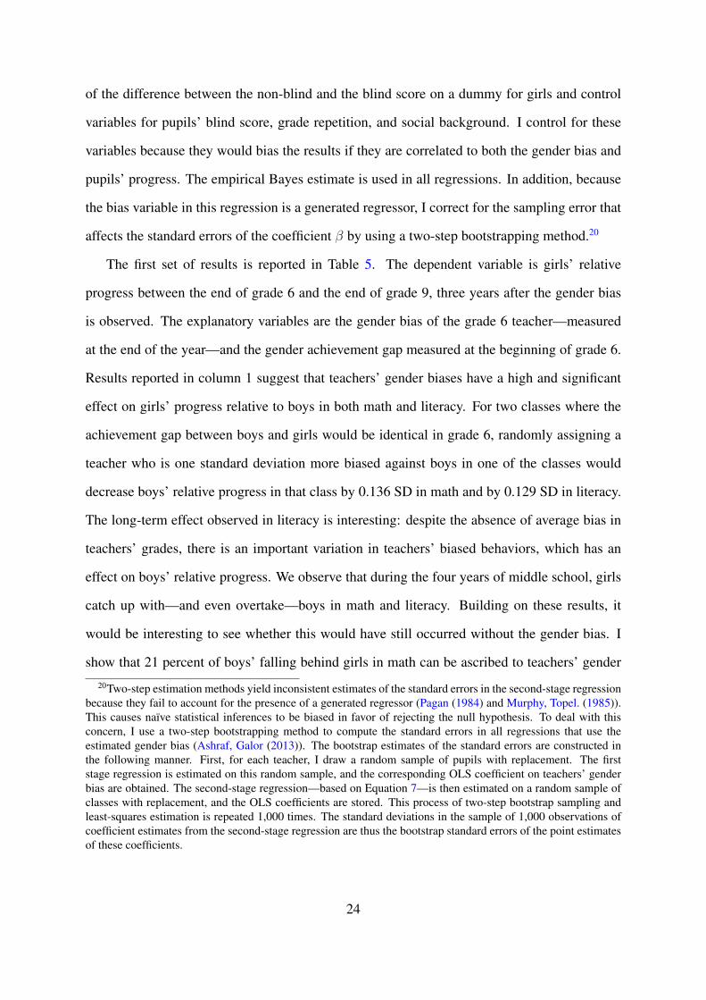
Figures 5 and 6 plot the distribution of boys’ and girls’ progress over middle school—
between the beginning of grade 6 and the end of grade 9. I define progress as the difference
between the blind score at the end of grade 9 and the blind score at the beginning of grade
6. Because both scores are standardized, a student’s progress corresponds to a higher ranking
over time in the score distribution. Graphically, there is clear evidence that boys progress less
than girls in mathematics, whereas progress in literacy is similar.13 Since girls’ blind scores
13At the beginning of grade 6, girls’ average math score is 0.075 points below the mean. It is only 0.021 pointsbelow the mean at the end of the 6th grade, and becomes 0.029 points above the mean by the end of grade 9, hence
8

were lower than boys’ at the beginning of grade 6, the faster progress experienced by girls
reduces the gap between boys’ and girls’ blind scores. By age 15, girls catch up with and even
overtake boys in both math and literacy. One of the objectives of this paper is to determine if
teachers’ biased behavior against boys can explain part of this differential progress in math and
the observed inequalities in choosing high schools and STEM courses.
II Model of Pupil’s Progress
I define a simple model aimed at isolating the effect of teachers’ gender biases on pupils’
progress. The main issue when evaluating the impact of grade biases on a pupil’s progress is
disentangling the effect of grade biases from several other determinants that might explain a
pupil’s progress and might be correlated to a teacher’s biased behavior. The following model
aims at isolating these various determinants of a pupil’s progress.
Equation 1 describes a blind score B1i given at the beginning of a period. The term blind
refers to a score given by an evaluator who has no identifying information about the student,
so the score should not be affected by any teacher’s stereotypes. This score is a noisy measure
of a student’s ability θ1i. εB1i captures the measurement error. Equation 2 describes a blind
score given to the same student at the end of the period. For the remainder of the model, all
variables and parameters referring to the end of the period are indexed by 2. A biased grade is
modeled as the difference between a student’s ability θi and the non-blind grade NBi given by
the teacher. At this stage of the model, a biased grade does not refer to a gender bias. It might
correspond to a teacher’s tough or lenient grading practice that applies to both genders.
B1i = θ1i + εB1i (1)
B2i = θ2i + εB2i (2)
Biasi = NBi − θi (3)
a total increase of 0.104 points of the SD.
9

A pupil’s ability has changed between the beginning and end of the period. I model this
evolution θ2i − θ1i as a function of the different effects I want to disentangle:
θ2i − θ1i = βBias1i + ηGi + µiTi + γθ1i + ωi (4)
Bias1i is the difference between a pupil’s ability and the grade given by the teacher.14 Ti is
a teacher effect. Teachers’ quality (also referred to as their value added) is intuitively correlated
to a student’s progress. In addition, the best teachers might also be more prone to encouraging
girls (or boys), so that teachers’ quality and gender biases would not be separately identified.
Including a teacher effect in the model allows us to disentangle a teacher effect from the gender
bias effect.
θ1i is a pupil’s achievement. A pupil’s initial level might be correlated to both his/her
progress and a teacher’s discriminatory behavior. Because low achievers have more room for
improvement, they might have a higher propensity to progress than their high-achieving coun-
terparts. In addition, pupils’ achievement could be correlated to teachers’ gender biases. Table
1 shows that girls perform worse than boys in the blind national evaluations in math. If teach-
ers try to encourage low performers by giving them relatively better grades, a bias in favor of
girls could partly capture this bias in favor of low performers. In that case, pupils’ achieve-
ment would be correlated to both teachers’ biases and pupils’ progress. Failure to take this into
account might bias the estimate of the effect of teachers’ biased behavior on pupils’ progress.
Gi is a dummy variable for girls. Girls’ unobserved characteristics should be taken into
account, as these characteristics might be correlated to both teachers’ gender biases and to their
progress: girls might have an intrinsic tendency to progress more than boys over the school
year, independent of any gender bias.
14The coefficient β captures several channels through which grade biases can affect a pupil’s progress. Mo-tivation or discouragement are direct channels, but effort is also an important channel, as are changes in self-confidence and the reduction of stereotype threats. I will not be able to distinguish between these different chan-nels, which are all captured by the coefficient β.
10

A pupil’s progress is measured by the evolution of his/her blind score over time :
B2i −B1i = θ2i + εB2i − θ1i − εB1i
= βBias1i + ηGi + µiTi + γθ1i + ωi + εB2i − εB1i
(5)
θ1i is replaced by (B1i − εB1i), which gives the following reduced-form equation:
B2i −B1i = β(NB1i −B1i) + ηGi + µiTi + γB1i + πvi + εB2i + (β − 1− γ)εB1i + ωi (6)
This equation isolates the different determinants of a pupil’s progress. The interpretation of
the coefficient β is straightforward: once controlled for a pupil’s ability B1i, girls’ tendency to
progress Gi and teacher quality Ti, β captures the effect of receiving a grade that is higher than
expected by a pupil’s ability.
However, there are two reasons why this individual-level equation is not the specification
I estimate. Firstly, and most importantly, the term (NB1i − B1i) captures a bias in teachers’
grades, but not a gender bias. Secondly, the estimate of its coefficient β would suffer from three
sources of endogeneity. An issue of reversed causality exists if teachers tend to be biased in
favor of the students they expect to have the highest potential for progress. In addition, because
the blind score is a noisy measure of a student’s ability, B1i is correlated to the error term εB1i.
This measurement error would yield an attenuation bias on β. Finally, the teacher effect Ti
might be correlated to the difference NB1i − B1i if the best teachers tend to have more tough
or lenient grading practices, for instance.
To obtain an estimate of teachers’ gender biases and circumvent the endogeneity concerns,
I use an alternative specification that consists of aggregating Equation 6 at the class level, for
both girls (G) and boys (B), and using a first-difference specification (between boys and girls).
The equation below, specified at the class level, corresponds to that new specification, which I
use to identify the effect of teachers’ gender biases on girls’ relative progress. The dependent
11

variable is the gap between girls’ and boys’ progress in class C:15
((B2G −B2B)− (B1G −B1B)
)c= η + β[(NB1G −B1G)− (NB1B −B1B)]c + γ(B1G −B1B)c + (ωG − ωB)c
(7)
(ProgresG − ProgresB)c = η + βGenderBiasc + γ(B1G −B1B)c + (ωG − ωB)c (8)
Thanks to the first-difference specification used, the simple difference (NB1i − B1i) becomes
a double difference (NB1G − B1G)− (NB1B − B1B), a frequent measure of gender biases in
teachers’ grades that has been introduced graphically in section I.B (Lavy (2008), Falch, Naper
(2013), Breda, Ly (2015), Goldin, Rouse (2000)). The gender bias is the difference between
girls’ and boys’ gap between the average non-blind and blind score.16 The assumptions behind
this methodology are provided in the next section. In this new aggregated specification, the
coefficient β identifies the effect of having a gender-biased teacher on girls’ relative progress.
The aggregation and first-difference specification also allows us to rule out the three endo-
geneity concerns observed in the individual-level specification. Because Equation 7 is specified
as a differentiation between boys’ and girls’ average scores at the class level, teacher effects
disappear as long as they are assumed to similarly affect boys and girls within a class. The first-
difference specification ensures that the effect of the gender bias I estimate is not explained by
a correlation between teachers’ value added and their biased behavior against boys. Using a
specification based on aggregated variables at the class level instead of at the individual level
also helps solve the measurement error concern on B1i. Averaging scores at the class level sig-15All variables are averaged conditionally to being a girl and having teacher Ti. Within a class, girls’ average
progress is given by:
E(B2i −B1i/Ti, Gi = 1) = γE(B1i/Ti, Gi = 1) + βE(NB1i −B1i/Ti, Gi = 1) + ηE(Gi/Ti, Gi = 1)
+µiE(Ti/Ti, Gi = 1) + E(ωi/Ti, Gi = 1) + E(εB2i/Ti, Gi = 1) + (β − γ − 1)E(εB1i/Ti, Gi = 1)
Replacing Gi = 1 by Gi = 0 in the above equation gives the symmetrical equation for boys.To simplify notations:
B2G = E(B2i/Ti, Gi = 1), B2B = E(B2i/Ti, Gi = 0)...
ωG = E(ωi/Ti, Gi = 1) + E(εB2i/Ti, Gi = 1) + (β − γ − 1)E(εB1i/Ti, Gi = 1)
ωB = E(ωi/Ti, Gi = 0) + E(εB2i/Ti, Gi = 0) + (β − γ − 1)E(εB1i/Ti, Gi = 0)
16It should be noted that this model refers to teachers’ biases related to students’ genders, but the same modelcould be used to study other sources of bias, such as those related to students’ social backgrounds or ethnicity.
12
nificantly reduces the measurement error affecting blind score measured at the individual level.
Finally, aggregation at the class level rules out concerns of a reversed causality at the individ-
ual level. Aggregation is, however, not sufficient, as reversed causality might also exist at the
class level. An additional assumption is required to rule out the latter: the assignment of pupils
to gender biased teachers must be “as good as random,” so that the students with an ex-ante
high potential for progress are equally distributed between classes. I test this assumption in the
section discussing the identification.
Grouped least square (GLS) on a set of class-aggregated means is equivalent to two-stage
least-squares (2SLS) using the interaction between teacher and girls as dummy instruments for
the gender bias in each class (Angrist, Pischke (2008)). As a result, standard instrumental vari-
ables assumptions apply. In particular, a central assumption of the identification—that pupils’
assignment to a gender biased teacher is random—will be analogous to an exclusion restric-
tion on these instruments. 2SLS appealing properties also apply to GLS. It notably provides
estimators that are robust to measurement error in explanatory variables (Angrist (1991)).
III Measuring Gender Biases in Teachers’ Grades
III.A Double-Difference Methodology
As stated in the previous section, using an aggregated and first-difference specification brings
out a double difference, which has been used in prior literature to measure gender biases in
teachers’ grades. Although the identification in this paper exploits the heterogeneity of this
gender bias across teachers (and not its average value), it is important to know if teachers tend
to favor a gender on average because it sheds light on the different patterns of progress between
boys and girls.
The double-difference methodology was introduced in a seminal paper by Blank (1991)
and used by Lavy (2008) to identify a bias in teachers’ grades. Later papers have also used this
double difference to estimate a gender bias: Falch, Naper (2013), Breda, Ly (2015), and Goldin,
Rouse (2000). The strategy consists of estimating the difference between boys’ and girls’
13

average gap between a non-blind and a blind score (NBi1−Bi1|Gi = 1)−(NBi1−Bi1|Gi = 0).
In the absence of teachers’ biases in grades, and under the assumption that both tests measure
the same abilities, the difference between the non-blind score and the blind score should be the
same for boys and girls: this corresponds to the common trend identification hypothesis. The
gender bias is estimated thanks to the following standard double-differences equation:
NBi −Bi = α0 + α2Gi + εi (9)
NBi is the non-blind score, Bi is the blind score, Gi is a dummy for girls, and εi is an
individual shock. The coefficient α2 provides an estimation of the gender biases in teachers’
grades and is equivalent to the double difference presented above and in Equation 7.
This coefficient can be interpreted as a gender bias in teachers’ grades if the blind and the
non-blind scores measure exactly the same skills, and if students’ unobserved characteristics
(such as stress) are equally shared by boys and girls. If the grades given by teachers measure
slightly different skills (homework for instance), for which boys or girls have an advantage,
then the double-difference should be interpreted more broadly as a bias in teachers’ evaluation
methods. Both assumptions are tested in further sections.
Finally, a last concern for the identification arises if the blind scores are not perfectly blind.
An important assumption for the DiD methodology is that the blind test scores do not contain
indications of the genders of the students. I cannot completely rule out the fact that some
graders might be able to use students’ handwriting to determine whether an exam is filled out
by a boy or a girl. But if the external correctors can identify a pupil’s gender, and if they suffer
from the same biases as teachers, the difference between the blind and the non-blind exam
would be attenuated. As a result, the DiD results I present in the next section would be a lower
bound.
14

III.B Estimation of Teachers’ Gender Biases
A more common formulation of DiD Specification 9 is written below. The estimate obtained
for the gender bias (α2) is identical but equation 10 has the advantage of providing coefficients
for the gender effect and the non-blind effect:
Scoin = α + βGi + γNBi + α2(Gi ∗NBi) + πc + εin (10)
Here Scoin is the grade received by a pupil when the nature of scoring is n (n=1 for non-blind
and 0 for blind). Hence, for each pupil, this dependent variable is a vector of both blind and
non-blind grades received. Gi is a dummy variable for girls. NBi is a dummy variable equal to
1 if the score has been given non-anonymously by a teacher.17 The coefficient of the interaction
term (α2) identifies a gender bias. Finally, for the results presented next, a class fixed effect
πc is included in the specification. This fixed effect is important to capture elements affecting
grades in a given class, such as teachers’ severity, student/teacher ratio, peer effects, or some
teachers being better at teaching girls than boys.
Table 2 presents the coefficient estimates of Equation 10. The first column presents the
results of the standard DiD specification without control variables. In all specifications, stan-
dard errors are estimated with school-level clusters to take into account common shocks at
the school level. In math, the coefficient of the interaction term Girl*Non-Blind is high and
significant—0.31 points of the SD—meaning that a strong bias against boys exists in this sub-
ject. Conditional on blind scores, boys’ non-blind scores are on average 6.2 percent lower than
girls in math at the beginning of grade 6. In literacy, the coefficient of the interaction term (not
shown) is neither high nor significant, meaning that no gender bias is observed in this subject.
We should keep in mind that the interpretation of this bias is relative: saying that teachers’
grades tend to be biased against boys in math is equivalent to saying that girls benefit from a
bias in their favor. In the remainder of the paper, I will sometimes use the term gender bias to
refer to the gender bias against boys.
17Note that NBi becomes a dummy in this specification, while it was a continuous variable (for test scores) inthe preceding equations.
15

These results confirm up to a point what Lavy (2008) observes in his analysis: despite the
commonly held belief that girls are discriminated against, the biases observed are in favor of
girls. Similarly, Robinson, Lubienski (2011) found that teachers in elementary and middle
schools consistently rate females higher than males in both math and reading, even when cog-
nitive assessments suggest that males have an advantage. Contrary to both previous studies,
I find a bias only in math and not in all subjects. The results of Breda, Ly (2015) are also
consistent with my estimates. They found that discrimination goes in favor of females in more
“male-connoted” subjects (e.g., math).
I check how pupils’ disruptive behavior, initial achievement, and grade repetition affect the
gender bias estimate. Taking this into account is important for the second part of the analysis,
as these variables could be correlated to both teachers’ gender bias and a student’s progress.
Results are presented in Appendix B: the gender bias is not explained by boys’ more disruptive
behavior or by them repeating more grades than girls. However, by running quantile regression,
I find that the largest gender bias is observed in the lowest decile of the blind scores (with a
coefficient of 0.327), while the smallest gender bias is observed in the highest decile of the
distribution (with a coefficient of 0.272). All results presented here are based on blind and non-
blind scores given at the very beginning of grade 6. To test if the gender bias is still observed at
the end of the year, I use the blind and non-blind grades given at the end of the school year and
replicate the analysis done above. Results are presented in Appendix C. Although the gender
bias is slightly smaller during the third term than during the first term, the effect of all control
variables remains very similar. Finally, results decomposed by teachers’ characteristics are also
provided in Appendix D.
IV Identification Strategy
The previous section presents estimates of the average value of the gender bias among all teach-
ers. The identification exploits the heterogeneity of this gender bias across teachers. More
specifically, the identification strategy is based on the observation that not all teachers are bi-
16

ased, and that among teachers who have a biased assessment of boys compared to girls, the
degree of the bias also differs across teachers, with some teachers being more biased than oth-
ers. I take advantage of both this heterogeneity in the degree of the bias and the quasi-random
assignment of pupils to teachers with different degrees of bias to test whether classes in which
students are randomly assigned a teacher who is highly biased against boys are also the classes
in which boys progress less (relative to girls). This identification strategy can be seen as a DiD
strategy, where the treatment corresponds to a gender bias against boys in some classes and the
outcome is boys’ progress compared to girls’.
IV.A Heterogeneity in Teachers’ Gender Bias
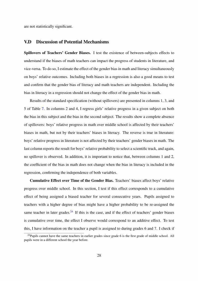
A simple visual way to test for the heterogeneity in teachers’ biased behavior is to plot this
variation in a graph. For each class in the sample, Graphics 7 and 8 display the gender bias
coefficient on the horizontal axis and girls’ progress relative to boys (during middle school)
on the vertical axis. The gender bias coefficient is defined as the double difference presented
earlier: the class average difference between the non-blind and the blind scores for girls, minus
this same difference for boys. The first noteworthy element is the high variation in the degree of
teachers’ gender biases. Observing a high variation in literacy is particularly interesting if we
keep in mind that, on average, we do not observe any bias against boys or girls in this subject.
Despite this null average, the high variation across classes in teachers’ biased assessments
might affect girls’ relative progress in these classes.
On the vertical axis, girls’ progress relative to boys is measured as the difference between
their blind score at the end of grade 9 and this blind score at the beginning of grade 6, minus this
same difference for boys. Graphically, there is clear evidence of a positive correlation between
the degree of teachers’ gender bias in favor of girls, and the degree of girls’ progress compared
to boys’.
17

IV.B Quasi-Random Assignment of Students to Biased Teachers
In Equation 7, the coefficient β identifies the effect of being assigned a teacher who is 1 SD
more biased against boys on boys’ average progress relative to girls’ after controlling for the
initial achievement gap between boys and girls. This coefficient can be seen as a causal effect
under the assumption that boys and girls’ assignment to a biased teacher is quasi-random. In
other words, being assigned a biased teacher is independent of students’ unobserved charac-
teristics that could be correlated to their progress. I use the term quasi-random to describe the
fact that pupils’ assignment to teachers is not done through a proper lottery. Yet, an arbitrary
assignment of girls or boys with high predicted progress to biased teachers is highly plausible.
Pupils considered in this study are in grade 6, which is the first year of middle school in France.
All students beginning grade 6 were enrolled in a different school the year before. Hence,
when deciding the composition of classes, school heads have very little information on these
new pupils. In particular, it is highly unlikely that school heads can predict students’ progress,
and therefore influence their assigned class and teacher. In addition, for school heads to assign
the most biased teachers to boys who are likely to progress less than girls, they would need to
know who the biased teachers are. This is again very unlikely.
Although it is not possible to test the assumption that pupils are randomly assigned to biased
teachers, I check if the assignment to a biased teacher is independent from boys’ and girls’
observed characteristics. I first regress the gender bias (defined at the class level in both literacy
and math) on pupils’ gender and find no significant effect: within a school, boys are not more
likely than girls to be assigned to math or literacy teachers with a high bias. Then, for boys and
girls separately, I successively regress math and literacy teachers’ estimated gender bias on the
following set of predetermined variables: score at the standardized test taken at the beginning
of grade 6, having upper-class parents, having lower-class parents, and having repeated a grade.
The coefficients are reported in Table 3. Each cell in the table corresponds to the coefficient
of a separate regression. In 13 regressions out of 16, the observed characteristics of boys
and girls are independent from being assigned a biased teacher. The only three exceptions do
not indicate a clear pattern of selection, which confirms students’ quasi-random assignment to
18

biased teachers.
The previous test rules out selection on observables. A second way to test the random
assignment—which also incorporates unobservable characteristics—is to check if the gender
bias of math teachers is correlated to the gender bias of literacy teachers. If teachers are as good
as randomly assigned, the biases of literacy and math teachers are expected to be completely
independent. I regress the gender bias in math on the gender bias in literacy to test if a between-
subject correlation in pupils’ experienced gender biases exists. I run this regression with one
observation per class, and I cannot reject the hypothesis that there is no correlation between the
biases in both subjects: the coefficient is 0.009 (SE=0.094).
IV.C Gender Bias and Students’ Unobserved Characteristics
The previous test is also important to show that the gender bias I measure does not capture
students’ unobserved characteristics. If the gender bias was incorporating information on stu-
dents’ unobserved characteristics, and if these unobserved characteristics are correlated to a
student’s progress, I would face an endogeneity issue. For instance, if girls’ characteristics
(such as test-taking habits, stress, or response to competitiveness18) tend to affect their blind
evaluations negatively, this would increase the double difference measure of the gender bias.
However, if these characteristics similarly affect girls’ (or boys’) evaluations in math and lit-
eracy, then we should observe a correlation between the measured bias of math and literacy
teachers (teaching the same students). The absence of correlation therefore brings one more
piece of evidence on the origin of the gender bias: it seems to be a pure teacher’s effect rather
than a bias driven by pupils’ characteristics.
An additional test can be done to further demonstrate that the gender bias I measure does
not capture boys or girls’ different unobserved characteristics. As stated above, any of these
characteristics that affect students equally in math and literacy will similarly affect the estimate
of the gender bias in these two subjects. For instance, in my setting, the competitiveness of the
18Recent studies suggest that girls tend to be relatively less effective than boys in environments that they per-ceive as more competitive (Gneezy et al. (2003)), or when the stakes of evaluations are higher (Azmat et al.(2016)).
19

environment and the stakes of the exams are identical for the math and literacy blind exams.
Based on this observation, I use an alternative methodology, based on a triple-difference (Breda,
Ly (2015)) rather than a double difference, to measure the gender bias. This methodology is
equivalent to implementing a within-gender between-subjects regression. It allows the response
to stakes or competitiveness to be distributed differently for boys and girls; however, this re-
sponse must be constant across subjects within gender. This within-gender between-subjects
method also controls for any characteristic specific to boys that potentially affects teachers’
biases similarly in all subjects: the fact that boys behave worse, might be less attentive, less
serious, and less diligent. As reported in Appendix E, the coefficient for relative bias obtained
with this method corresponds to the coefficient in math minus the one in literacy, hence 0.291.
This is extremely similar to the DiD estimate, which confirms that the gender bias I measure
with the DiD methodology does not capture students’ unobserved characteristics.
Finally, even if boys and girls were reacting differently to stress, competitiveness, or the
stakes of the exams, this would not affect the estimate of interest (the effect of teachers’ gender
biases on students’ progress), as long as the assignment of boys or girls who are more stressed
is quasi-random. The quasi-random assignment, tested in the previous section, helps to rule out
any selection pattern on unobserved characteristics.
IV.D Interpretation of the Gender Bias
In my setting, the blind and the non-blind scores might have different formats. In this paper,
blind tests are standardized tests created by the French Education Ministry, while non-blind
grades correspond to the average mark given every term by the teacher. Although both are
designed to measure the same competencies (as explained when presenting the data), we cannot
completely rule out small differences in the content or forms of the exams. In particular, the
grades given by teachers might encompass some homework. This would not be an issue if
the difference in the evaluation methods (the quantity of homework given) was constant across
classes. Having no information on the evaluation practices of teachers, I cannot rule out the fact
that some teachers use evaluation methods that focus more on skills at which girls are better
20
than boys. Hence, the variation across classes of the double-difference estimate of teachers’
biases might capture differences in their evaluation methods.
The gender bias might also capture teachers’ biased behavior in addition to their biased
grading practices. Teachers who tend to be biased against boys in their grades might also
engage in other unobserved classroom practices that make boys less likely to succeed. They
might be less encouraging, less friendly, focus less attention on boys, or be more critical. This
concern is particularly true when measuring the gender bias at the very beginning of grade 6
and in measuring students’ progress during grade 6 (between September and June) because
pupils experience the gender bias in grades at the beginning of the year and then potentially
experience the biased behavior of their teacher throughout the entire year. A way to disentangle
these two effects is to use the bias in grades measured at the end of the grade 619—instead of the
beginning—and pupils’ progress between the beginning of grade 7 and the end of grade 9. This
ensures that the progress is measured over a period when pupils are less affected by the biased
behavior of their teacher. Hence, in the forthcoming analysis of student’s progress, I use the
bias measured at the end of grade 6. This seems preferable, but if a teacher’s biased behavior
has a persistent effect on students, this solution does not allow us to completely disentangle
both effects.
To summarize, the effect of gender bias on progress and other outcomes is likely to capture
a bias in teachers’ grading practices, but also in their evaluation practices and potentially in
their behavior. Even without being able to separately identify these elements, it is interesting
to know if teachers’ biased evaluation practices—with all the elements they embed—have an
impact on boys’ progress relative to girls’.
IV.E Balance Check of Attrition
Three different outcomes are used to estimate the causal effect of teachers’ gender biases on
students : the blind score at the end of grade 9, the school attended during grade 10, and pupils’
19Both the blind and non-blind scores have been collected at the beginning of grade 6, but also at the end of thesame academic year.
21
subject choices during grade 11. Two types of attrition exist: an attrition at the class level, when
scores are missing for all pupils in a class, and an attrition at the individual level, when scores
are missing for some pupils within a class. There is no attrition at the class level in my sample:
all classes for which the bias is estimated at the end of grade 6 are observed in grades 10 and
11. The second type of attrition exists, but it would only be problematic if student attrition is
correlated to the bias of teachers. To test this, I check if the percentage of girls or boys missing
in a class is correlated to the degree of bias of their teacher. I regress the percentage of girls
missing (per class) on the gender bias. This is done successively for boys and girls. For each
gender, six different regressions are run (corresponding to the six columns of Table 4), where
each of the potentially missing variables are successively the dependent variable: blind score
in literacy and math at the end of grade 9, information on school choice during grade 10, and
information on course choice during grade 11. None of the coefficients are significant.
V Empirical Results
V.A Empirical Bayes Estimates of Teacher Bias
A last concern when estimating measures of teachers’ gender biases involves estimation error
arising from sampling variation. With small samples, a few students can have a large impact on
test scores. In my sample, the average number of students per teacher is 36.3 in math and 31.8 in
literacy. At the school level, Kane, Staiger (2002) found that among the smallest schools, more
than half (56 percent) of the variance in mean gain scores is due to sampling variation and other
non-persistent factors. In the presence of sampling error, the estimated teacher bias tj is the
sum of the true teacher bias θj plus some error εj , where εj is uncorrelated with tj . The variance
of the estimated teacher biases has two components: the true variance of the teacher bias and
the average sampling variance. Without accounting for it, the estimation error would lead to
attenuation bias when I use the teacher bias measure in regressions as an explanatory variable
for students’ progress. To address this problem of sampling error, I construct empirical Bayes
estimates of teacher gender bias. This approach was suggested by Kane, Staiger (2002) for
22

measures of schools’ accountability measures. The basic idea of the empirical Bayes approach
is to multiply a noisy estimate of each teacher bias by an estimate of its reliability. Thus,
less reliable estimates are shrunk back toward the mean (0, since the teacher estimates are
normalized to be mean 0). Several recent applications have used this methodology to estimate
teacher value added (Jacob, Lefgren (2005), Kane, Staiger (2008), Chetty et al. (2014)). For
each teacher, the reliability ratio of the noisy estimate of the gender bias is the ratio of signal
variance to signal plus noise variance, where the noise corresponds to the squared standard-
error of the bias estimate. It is relatively simple to estimate this ratio by using the observed
estimation error from each teacher bias estimation. We obtain a measure of the true variance
V (θ) by subtracting the mean error variance (the average of the squared standard errors of the
estimated teacher bias) from the variance of the observed bias: V (θ) = V (t)− E[V (εj)].
RRj =V (θ)
V (θ) + V (εj)=
V (t)− E[V (εj)]
V (t)− E[V (εj)] + V (εj)(11)
Finally, I construct an empirical Bayes estimator of each teacher’s bias by multiplying the initial
bias estimate by an estimate of its reliability: tEBj = tj ∗ RRj . After adjusting for estimation
error, the standard deviation of teacher bias is 0.047 in math and 0.112 in literacy. Before
the shrinkage, these SDs were equal to 0.25 and 0.37, which shows that most of the variation
between teachers in the degree of the estimated bias is due to sampling noise. The adjusted
estimators of teachers’ gender biases will be used in all forthcoming regressions of students’
progress on teachers’ biases. Jacob, Lefgren (2005) showed that using the empirical Bayes
estimates as an explanatory variable in a regression yields point estimates that are unaffected
by the attenuation bias that would result from using standard OLS estimates.
V.B Effect of Teachers’ Gender Biases on Progress
The first regression is based on Equation 7. The double difference on the right-hand side
of the equation corresponds to teachers’ gender bias estimated class by class. In the following
empirical analysis, the coefficient used for the gender bias is obtained by running the regression
23
of the difference between the non-blind and the blind score on a dummy for girls and control
variables for pupils’ blind score, grade repetition, and social background. I control for these
variables because they would bias the results if they are correlated to both the gender bias and
pupils’ progress. The empirical Bayes estimate is used in all regressions. In addition, because
the bias variable in this regression is a generated regressor, I correct for the sampling error that
affects the standard errors of the coefficient β by using a two-step bootstrapping method.20
The first set of results is reported in Table 5. The dependent variable is girls’ relative
progress between the end of grade 6 and the end of grade 9, three years after the gender bias
is observed. The explanatory variables are the gender bias of the grade 6 teacher—measured
at the end of the year—and the gender achievement gap measured at the beginning of grade 6.
Results reported in column 1 suggest that teachers’ gender biases have a high and significant
effect on girls’ progress relative to boys in both math and literacy. For two classes where the
achievement gap between boys and girls would be identical in grade 6, randomly assigning a
teacher who is one standard deviation more biased against boys in one of the classes would
decrease boys’ relative progress in that class by 0.136 SD in math and by 0.129 SD in literacy.
The long-term effect observed in literacy is interesting: despite the absence of average bias in
teachers’ grades, there is an important variation in teachers’ biased behaviors, which has an
effect on boys’ relative progress. We observe that during the four years of middle school, girls
catch up with—and even overtake—boys in math and literacy. Building on these results, it
would be interesting to see whether this would have still occurred without the gender bias. I
show that 21 percent of boys’ falling behind girls in math can be ascribed to teachers’ gender
20Two-step estimation methods yield inconsistent estimates of the standard errors in the second-stage regressionbecause they fail to account for the presence of a generated regressor (Pagan (1984) and Murphy, Topel. (1985)).This causes naïve statistical inferences to be biased in favor of rejecting the null hypothesis. To deal with thisconcern, I use a two-step bootstrapping method to compute the standard errors in all regressions that use theestimated gender bias (Ashraf, Galor (2013)). The bootstrap estimates of the standard errors are constructed inthe following manner. First, for each teacher, I draw a random sample of pupils with replacement. The firststage regression is estimated on this random sample, and the corresponding OLS coefficient on teachers’ genderbias are obtained. The second-stage regression—based on Equation 7—is then estimated on a random sample ofclasses with replacement, and the OLS coefficients are stored. This process of two-step bootstrap sampling andleast-squares estimation is repeated 1,000 times. The standard deviations in the sample of 1,000 observations ofcoefficient estimates from the second-stage regression are thus the bootstrap standard errors of the point estimatesof these coefficients.
24

bias against them.21
When interpreting the previous coefficients, we should keep in mind that the effect is rela-
tive: saying that teachers’ gender biases reduces boys’ relative progress is equivalent to saying
that it increases girls’ relative progress. For a matter of consistency, I will systematically use
the first construction. As the outcome corresponds to the difference between girls’ and boys’
progress, the positive coefficient I find could correspond to higher progress for girls than for
boys, or a blind score that remains constant for girls over time but decreases for boys (due to
their feeling of being negatively discriminated against compared to girls, for instance). As ex-
plained in section II, this first-difference specification ensures that my estimates do not capture
the effect of teachers’ quality, which might be correlated to a teacher’ gender bias. It is still
interesting to present the results separately for boys and girls, although the specification is a
bit less convincing in terms of identification. This helps with answering an important question:
does the gender bias help girls or hurt boys? The results suggest that having a math teacher
who is one SD more biased against boys does not impact boys’ progress but significantly in-
creases girls’ progress (coef=0.124, SE=0.043). On the other hand, in literacy, having a biased
teacher significantly reduces boys’ progress (coef=-0.061, SE=0.042) but positively impacts
girls’ progress (coef=0.067, SE=0.042), although the coefficients are not significant.22
21The descriptive statistics presented in Table 1 show that at the beginning of grade 6, the gap between girls’and boys’ blind math scores favors boys and equals -0.147 points of the SD. By the end grade 9, the achievementgap is in favor of girls and equals -0.058 SD. Over the four years of middle school, this represents a relative fallingbehind of boys compared to girls of 0.205 SD. The results reported above suggest that going from no gender biasto the average estimate of teachers’ bias makes boys progress 0.043 points less than girls.
22The differences observed between subjects and genders are consistent with a simple model that would takeinto account two parameters: (1) the importance attached to grades (assumed to be higher for girls than for boys)and (2) the lack of self-confidence (assumed to be higher in literacy for boys and in math for girls). If students aremore impacted by encouragement in a subject where they lack self-confidence, we would intuitively expect a biasin math and literacy to impact boys and girls differently. Indeed, a bias against boys in math would hardly impactboys’ performance in math (as they do not attach much importance to grades and do not lack self-confidence inmath), but it would strongly boost girls’ performance (as they both attach more importance to grades and lack self-confidence in math). This is what my estimates suggest. On the other hand, a bias against boys in literacy wouldnow impact boys negatively, as they tend to lack self-confidence in that subject, while boosting girls’ performanceless (as they still attach importance to the grade but do not lack self-confidence in literacy). Again, this is exactlywhat my estimates suggest.
25

V.C Effect of Teachers’ Gender Biases on Course Choice
Grade 9 is the last grade of middle (and compulsory) school. After this grade, pupils can choose
between a vocational, technical, or general high school. The majority of students select general
high school because it provides the most opportunities to continue studies at university. In our
sample, 50.9 percent of girls chose a general high school, as did 40.3 percent of boys. This
highly unbalanced statistic raises a first question: do teachers’ gender biases impact the type
of high school boys choose compared to girls? Then, for the pupils who decide to attend a
general high school, everyone attends the same courses during grade 10, but pupils have to
specialize when they enter grade 11. Three options are available to them: sciences, humanities,
or economics and social sciences. In this sample, among girls in general high school, 32.8
percent chose the scientific course, while 40.2 percent of the boys did so. This reversal of the
gender probability is striking, as the scientific path is the most prestigious one, and the one that
leads to higher education in science, technology, engineering, and math (STEM) fields. These
fields of study are highly gender-unbalanced in most countries, which raises a second question:
do teachers’ gender biases impact the relative probability that girls enroll in scientific courses?
Using the same specification as before, I successively analyze the effect of teachers’ gender
biases during grade 6 on four outcomes: boys’ relative probability to attend a general high
school, to choose a scientific course, to choose a literature course, and to repeat a grade. Results
are presented in Table 6. All regressions are run on all pupils to avoid any selection effect.
For instance, the regression of the probability to choose a scientific course in grade 11 is not
conditional on attending a general high school.
I find that being assigned a teacher who is one SD more biased against boys in grade 6
decreases boys’ relative probability to attend a general high school (rather than a professional or
technical one) by 1.5 percentage points, although that coefficient is not statistically significant.
This is true when the bias is in math or in literacy. One of the drawbacks of this analysis is the
limited number of observations available, which makes it more difficult to detect an effect. The
bootstrap method significantly increases the standard-errors value, so that several coefficients
are not significant, despite having a sign that is sensible. For instance, a back-of-the-envelope
26

calculation confirms the sign and the size of the effect on boys’ relative probability to select a
general high school. I find that having a teacher who is 1 SD more biased against boys in math
decreases their relative progress by 0.136 SD (Table 5), and a simple regression shows that a
one-SD drop in boys’ relative achievement at the end of middle school reduces their relative
probability to attend a general high school by 20.7 percentage points. By combining these two
effects, I get an upper-bound effect of a biased teacher on boys’ relative probability to attend
a general high school of 0.028. This is in line with the coefficient I obtain in the first column
of Table 6 (0.015).23 Knowing that, on average in this sample, boys are 10.6 percentage points
less likely than girls to attend a general high school, having a teacher who is one SD more
biased against boys would increase this gap by one and one half points (14 percent).
The results reported in columns 3 and 4 suggest that teachers’ biases in math positively
affect girls’ relative probability to choose a scientific course during grade 11. More precisely,
having a teacher who is one SD more biased in favor of girls increases girls’ probability to
select a scientific track by 2.7 percentage points compared to boys. This would reduce by
36 percent the gap between boys’ and girls’ probability to choose a scientific track, which is
initially 7.4 percentage points. This observation is interesting, as the scientific path is the most
prestigious one, and the one that leads to higher education in STEM fields. This result is in line
with Lavy, Sand (2015), who found that "the estimated effect of math teachers’ stereotypical
attitude [in favor of boys] on enrollment in advance studies in math is positive and significant
for boys (0.093, SE=0.049) and negative and significant for girls (-0.073, SE=0.044)."
It is also interesting to calculate what share of the observed gender gap in scientific course
choice is due to the average value of teachers’ gender biases in math (estimated around 0.32
points of a SD). Teachers’ average biases in math contribute to a reduction of 11.7 percent of
the gender gap in scientific course enrollment.
Finally, it is worth noting that the biases of literacy teachers have no impact on girls’ relative
probability to select a scientific track in grade 11. Teachers’ biases against boys in math and
literacy seem to increase boys’ relative probability to repeat a grade, although the coefficients
23I refer to this as an upper bound due to the high endogeneity in the second regression of boys’ relativeprobability to attend a general high school on their relative achievement at the end of middle school
27
are not statistically significant.
V.D Discussion of Potential Mechanisms
Spillovers of Teachers’ Gender Biases. I test the existence of between-subjects effects to
understand if the biases of math teachers can impact the progress of students in literature, and
vice-versa. To do so, I estimate the effect of the gender bias in math and literacy simultaneously
on boys’ relative outcomes. Including both biases in a regression is also a good means to test
and confirm that the gender bias of literacy and math teachers are independent. Including the
bias in literacy in a regression should not change the effect of the gender bias in math.
Results of the standard specification (without spillovers) are presented in columns 1, 3, and
5 of Table 7. In columns 2 and 4, I regress girls’ relative progress in a given subject on both
the bias in this subject and the bias in the second subject. The results show a complete absence
of spillovers: boys’ relative progress in math over middle school is affected by their teachers’
biases in math, but not by their teachers’ biases in literacy. The reverse is true in literature:
boys’ relative progress in literature is not affected by their teachers’ gender biases in math. The
last column reports the result for boys’ relative probability to select a scientific track, and again,
no spillover is observed. In addition, it is important to notice that, between columns 1 and 2,
the coefficient of the bias in math does not change when the bias in literacy is included in the
regression, confirming the independence of both variables.
Cumulative Effect over Time of the Gender Bias. Teachers’ biases affect boys’ relative
progress over middle school. In this section, I test if this effect corresponds to a cumulative
effect of being assigned a biased teacher for several consecutive years. Pupils assigned to
teachers with a higher degree of bias might have a higher probability to be re-assigned the
same teacher in later grades.24 If this is the case, and if the effect of teachers’ gender biases
is cumulative over time, the effect I observe would correspond to an additive effect. To test
this, I have information on the teacher a pupil is assigned to during grades 6 and 7. I check if
24Pupils cannot have the same teachers in earlier grades since grade 6 is the first grade of middle school. Allpupils were in a different school the year before.
28

the probability that a pupil is assigned the same teacher during grade 7 is correlated to his/her
teachers’ gender biases.25 The results suggest that being assigned a grade 6 teacher with a
one-SD higher gender bias increases a pupil’s probability to be reassigned to the same teacher
in grade 7 by 4.1 percentage points in math (SD = 0.004), but decreases a pupil’s probability
by 2.5 percentage points in literacy (SD = 0.05). Both coefficients are statistically significant,
and the estimates are very similar for boys and girls. Then I check if the effect of the bias is
cumulative over the years—in other words, if being reassigned a biased teacher further impedes
boys’ relative progress. For each class, I calculate the percentage of pupils in the class that are
reassigned to the same teacher in grade 7. I add this variable, and its interaction with the gender
bias, to the specification used previously. The results presented in Table 8 clearly indicate that
the effect of teachers biases is not cumulative over time: the interaction term added is close to
0 in math and literacy. Being re-assigned the same biased teacher does not further reduce boys’
relative progress. This result is not so surprising if we think that students might become aware
of the gender biases of their teachers, so that the effect fades out. If effort and achievement are
substitutes, boys could even increase their effort once they realize that they perform relatively
poorly compared to girls.
Contrast Effects, Stereotype Threat, and Mistrust. Finally, prior research can help to in-
terpret my results. Some papers highlight a "contrast effect" according to which a student’s aca-
demic self-concept is positively influenced by his or her individual achievement, but negatively
affected by other peers’ average achievement—usually composed of peers in the classrooms—
once controlled for individual achievement (Murphy, Weinhardt (2013), Trautwein et al. (2006),
Marsh, Craven (1997)). This helps to explain why a gender bias in a given subject—which is
a bonus for girls compared to their male peers—could increase girls’ progress in this subject,
but reduce boys’. Positively rewarding girls, relative to boys, could also reduce the stereotype
threat effect. In situations where stereotypes are perceived as important, some girls have been
proven to perform poorly for the sole reason that they fear confirming the stereotypes (Spencer
25More specifically, I regress a dummy indicating if a pupil has the same teacher during grades 6 and 7 on thegender bias of the grade 6 teacher. This regression is done on a sample of 3761 pupils for which I have informationon their grade 7 teacher.
29

et al. (1999)). If math is perceived by girls as highly affected by teachers’ stereotypes, over-
grading girls in this subject would be expected to reduce their anxiety of being judged as poor
performers, and therefore favor their progress in math. Reversely, if boys become aware of the
gender biases of their teachers, they might develop behavior that confirms that bias. Finally,
if teachers’ gender biases are too obvious during grade 6, boys and girls might increasingly
mistrust their grades. Mechtenberg (2009) suggests that girls are reluctant to internalize good
grades in math because they believe their grades are biased.
VI Robustness Checks
First, I run a placebo test where teachers are randomly assigned to different classes. Running
the standard regression with boys’ relative progress as a dependent variable in both math and
literature gives insignificant coefficients in both subjects (in math: β = −0.032, SD=0.027,
while in literature: β = −0.019 and SD=0.036).
VI.A Are Both Tests Measuring the Same Abilities?
As explained in the section on double differences, one of the key assumptions behind the DiD
methodology is that blind and non-blind scores measure the same abilities. If this is not the
case, and if boys or girls were more endowed in an ability measured more by the class exam,
then the double difference would not capture only teachers’ gender biases. It would also poten-
tially capture boys’ or girls’ particular skills measured by one of the scores (including home-
work, for instance). As mentioned earlier, the fact that the blind and the non-blind scores do not
measure the same skills would not bias my estimate as long as the differences in the abilities
measured do not vary between teachers. I have adopted a conservative approach so far by say-
ing that I could not completely rule out that grades given by teachers might encompass slightly
different skills from the standardized tests, and that this skill difference might also vary across
teachers, with some teachers giving more homework. A way to rule out this concern is to show
that grades given by teachers and standardized evaluations are measuring the same skills.
30

To do so, I define a simple model that describes how blind and non-blind scores are at-
tributed. The main assumption of this model is that blind scores are free of any bias and mea-
sure only a pupil’s ability, whereas non-blind scores can be affected by teacher’s stereotypes
toward boys or girls. Hence, blind scores are modeled as a function of a pupil’s ability only:
Bi = θ1i + εiB (12)
θ1i is a pupil’s ability, Bi is a noisy measure of a pupil’s ability, and εiB corresponds to an
individual random shock specific to blind scores. This might capture any effect that makes a
pupil overperform or underperform the day of the exam and can be interpreted as measurement
error. Non-blind scores can be affected by teachers’ beliefs toward pupils’ genders. Hence,
they can be modeled as a function of both a pupil’s ability and his/her gender:
NBi = α0 + θ2i + α2Gi + εiNB (13)
θ2i is the pupil’s ability that is measured by the non-blind test. Gi is a dummy variable
for girls. α2 is the coefficient capturing the potential gender bias. εiNB is an individual shock
specific to grades attributed by teachers. This noise might capture pupils’ behavior, for instance.
Finally, I allow θ1i and θ2i to differ, meaning that abilities measured by blind and non-blind
scores might differ. The relationship between both abilities can be modeled as follows:
θ2i = ρθ1i + vi (14)
vi captures variables that potentially affect ability measured by class exams θ2i, once con-
trolled for ability measured by blind score θ1i. Any specific ability measured by class exams
but not by standardized tests would be captured by vi. The skills measured by blind scores (θ1i)
might include pupils’ long-term memory and their ability to synthesize knowledge acquired
in the last few months, while ability measured by non-blind scores (θ2i) might integrate more
short-term skills, such as homework or learning an exercise by heart and replicating it the day
31

after for the class exam.26 The reduced form of this structural model is obtained by replacing
θ2i by its formula in equation 13, and by replacing θ1i by (Bi − εiB):
NBi = α0 + ρBi + α2Gi + (εiNB + vi − ρεiB) (15)
The DiD specification discussed in Section III rests on the assumption that both tests mea-
sure the same abilities. In Equation 15, this is equivalent to ρ = 1 and vi = 0. A first way to
test if both scores measure the same abilities is to directly estimate the reduced-form Equation
15, in which no restrictive assumption is imposed on abilities, and to verify if the coefficient ρ
is significantly different from 1. If not, both tests can be assumed to measure abilities that are
very similar. Due to the measurement error affecting the blind score, an instrumental variable
approach is used for this estimation, where the blind score is instrumented by a student’s month
of birth. The method and results are fully detailed in Appendix F. As reported in Table A.6, the
IV coefficient of the blind score ranges from 0.964 in literacy to 1.090 in math. In both cases,
I cannot reject the hypothesis that ρ = 1. This result suggests that the blind and non-blind tests
measure skills that are very similar, and hence that using the double-difference methodology
provides estimates of the gender bias that do not capture differences in the skills measured.27
A second way to test if both scores measure the same abilities is to regress boys’ and girls’
ranks in the blind score on their ranks in the non-blind score. Intuitively, if the standardized
evaluation and the class exams measure the same competencies, we would expect pupils’ ranks
to be the same for both exams. Running the aforementioned regressions confirms this. For
girls, the coefficient of the regression is equal to 1 (SD=0.007), suggesting a very high corre-
lation between their ranks in the blind and the non-blind scores. For boys, the estimate equals
0.86 (SD=0.007). Using the Spearman’s rank correlation leaves the results unchanged. The
coefficient equals 0.75 for girls and 0.76 for boys.
26This way of modeling blind and non-blind scores is highly simplified and relies on two important hypotheses.I suppose a linear relation between non-blind scores, ability, and gender, and I assume that non-blind scores do notdepend on blind scores in this specification. This hypothesis is likely to be satisfied in our context because blindtests were not graded by teachers but by independent correctors.
27In addition, the IV estimate of the gender bias coefficient (α2) equals 0.339 in math and 0.080 in literacy,which is very similar to the coefficients obtained by implementing DiD.
32

VI.B Time Lag between the Date of the Blind and Non-Blind Scores
The blind and the non-blind scores are not taken exactly at the same date, which can affect
my estimates. As mentioned before, the dataset includes a blind and non-blind score from the
beginning and end of grade 6. Yet for both periods, a time lag exists between the date when
the national evaluation is taken and the date when the grades are given by teachers. For all
regressions presented before, the gender bias is estimated based on scores given at the end
of the school year. Pupils take the standardized blind test during one of the last days of the
school year, while teachers’ assessments are an average of several grades given by teachers
between April and mid-June (last term of the academic year). Since the last term lasts three
months, this average of several grades measures a pupil’s average ability about one and a half
months before the end of the school year in mid-June. This time lag between the dates of
the blind and non-blind scores might be problematic if girls tend to progress more than boys
during this period, especially if girls’ better progress is higher in classes where teachers are
more biased. Yet, because the blind score is measured after the non-blind score, the double-
difference coefficient, which captures the gender bias, would be a lower bound for the true
gender bias if girls tend to progress more. Most importantly, the higher the gender bias of a
teacher, the larger the downward bias, so that the time lag would tend to shrink the variance of
the gender bias. As a result, my estimates would tend to underestimate the impact of teachers’
gender biases on students’ progress and subsequent outcomes.28
VII Conclusion
A number of papers have shown that teachers’ stereotypes can bias their assessment and grades,
yet none of these papers has gone one step further by studying the impact of teachers’ gender
biases on students’ subsequent progress and schooling trajectories. The main contribution of
28The direction of the bias would be opposite if the scores collected at the beginning of the year had been usedto estimate gender bias. At the beginning of the year, the time lag is reversed: pupils take the standardized blindtest during one of the first days of the school year, whereas teachers’ assessments are an average of several gradesgiven by teachers during the three first months.
33

this paper is to answer this question by using a new identification strategy based on the varia-
tion of gender biases between teachers and the quasi-random assignment of students to these
different teachers. To measure gender biases, I use a standard double-difference methodology
that exploits the availability of both blind and non-blind scores for each student.
The key finding is that teachers’ gender biases have a high and significant effect on girls’
progress relative to boys’ in both math and literacy. Over middle school, teachers’ gender bias
against boys explains 21 percent of boys falling behind girls in math. Although students who
are assigned a more biased teacher in grade 6 are more likely to be reassigned the same teacher
in grade 7, boys’ relative progress is not lower for these students. Moving to other outcomes,
I find that having a teacher who is one SD more biased in math increases girls’ probability to
select a scientific track in high school by 2.7 percentage points compared to boys’. Teachers’
average bias in math contributes to a reduction of 11.7 percent of the gender gap in choosing
scientific courses.
I use a dataset that has been collected from schools in a relatively deprived educational
district in France. This should be kept in mind when interpreting the results and for the exter-
nal validity of this analysis. Teachers assigned to deprived areas are on average younger than
teachers in more advantaged schools, and we have seen that inexperienced teachers are more bi-
ased. Similarly, pupils in these areas might face more constraints (financial or self-censorship)
regarding their schooling decisions.
An interesting follow-up would be to understand the channels through which a gender bias
affects boys’ relative achievement. Positively rewarding pupils could provide motivation, lead
to increased efforts and self-confidence, and reduce the effects of stereotype threat. On the other
hand, if pupils consider effort and abilities as substitutes, a higher grade might be an incentive
to reduce effort and work. Unfortunately, I am not able to disentangle these effects, which
might compensate or reinforce each other. This is an interesting question for future research.
It would also be worthwhile to extend this analysis by using an exhaustive sample of students,
ensuring that the sample is large enough to detect small effects. Indeed, one of the drawbacks
of my analysis is the limited number of observations available, which makes it more difficult to
34

detect an effect.
This analysis provides policy-relevant results. Teachers’ gender biases can have a strong
impact on the achievement gap between boys and girls. This provides a new explanation for
boys increasingly falling behind girls at school and for girls choosing relatively fewer scientific
courses in high school. These findings open the door to new policies. If the main objective of
policy-makers was to reduce achievement gaps—whether between boys and girls or students
from different ethnicities or social backgrounds—teachers’ evaluation methods and behavior
could be considered as an instrument to achieve that goal.
ReferencesAngrist Joshua D. Grouped-data estimation and testing in simple labor-supply models // Journal
of Econometrics. 1991. 47, 2. 243 – 266.
Angrist Joshua D., Krueger Alan B. Does Compulsory School Attendance Affect Schoolingand Earnings? // The Quarterly Journal of Economics. 1991. 106, 4. 979–1014.
Angrist Joshua D, Pischke Jörn-Steffen. Mostly Harmless Econometrics: An Empiricist’s Com-panion. 2008.
Apperson Jarod, Bueno Carycruz, Sass Tim. Do the Cheated Ever Prosper? The Long-runEffects of Test-Score Manipulation by Teachers on Student Outcomes // Working Paper No.155. 2016.
Ashraf Quamrul, Galor Oded. The ’Out of Africa’ Hypothesis, Human Genetic Diversity, andComparative Economic Development. // American Economic Review. 2013. 103, 1. 1–46.
Autor David, Figlio David, Karbownik Krzysztof, Roth Jeffrey, Wasserman Melanie. SchoolQuality and the Gender Gap in Educational Achievement // SEII Working Paper. 2016. 1.
Avvisati Francesco, Gurgand Marc, Guyon Nina, Maurin Eric. Getting Parents Involved : aField Experiment in Deprived Schools // Review of Economic Studies. 2014. 81, 1. 57–83.
Azmat Ghazala, Calsamiglia Caterina, Iriberri Nagore. Gender Differences in Response toBig Stakes // Journal of the European Economic Association. 2016.
Bar Talia, Zussman Asaf. Partisan grading // American Economic Journal: Applied Economics.2012. 4, 1. 30–48.
Bedard Kelly, Dhuey Elizabeth. The Persistence of Early Childhood Maturity: InternationalEvidence of Long-Run Age Effects // The Quarterly Journal of Economics. 2006. 121, 4.1437–1472.
35

Bertrand Marianne, Pan Jessica. The Trouble with Boys: Social Influences and the GenderGap in Disruptive Behavior // American Economic Journal: Applied Economics. 2013. 5, 1.32–64.
Blank Rebecca M. The Effects of Double-Blind versus Single-Blind Reviewing: ExperimentalEvidence from The American Economic Review // The American Economic Review. 1991.81, 5. 1041–1067.
Bonesrønning Hans. The Effect of Grading Practices on Gender Differences in AcademicPerformance // Bulletin of Economic Research. 2008. 60, 3. 245–64.
Breda Thomas, Ly Son Thierry. Professors in Core Science Fields Are Not Always Biasedagainst Women: Evidence from France // American Economic Journal: Applied Economics.2015. 7, 4. 53–75.
Buckles Kasey S., Hungerman Daniel M. Season of Birth and Later Outcomes: Old Questions,New Answers // Review of Economics and Statistics. 2012. 95, 3. 711–724.
Burgess Simon, Greaves Ellen. Test Scores, Subjective Assessment, and Stereotyping of EthnicMinorities // Journal of Labor Economics. 2013. 31, 3. 535–576.
Chetty Raj, Friedman John N., Rockoff Jonah E. Measuring the Impacts of Teachers I: Evalu-ating Bias in Teacher Value-Added Estimates. // American Economic Review. 2014. 104, 9.2593–2632.
Cornwell Christopher, Mustard David B., Parys Jessica Van. Noncognitive Skills and the Gen-der Disparities in Test Scores and Teacher Assessments: Evidence from Primary School //Journal of Human Resources. 2013. 48, 1. 236–264.
Crawford Claire, Dearden Lorraine, Meghir Costas. When You Are Born Matters: The Impactof Date of Birth on Child Cognitive Outcomes in England // CEE Discusion Paper. 2007.
Cunha Flavio, Heckman James J. Formulating, Identifying and Estimating the Technology ofCognitive and Noncognitive Skill Formation // Journal of Human Resources. 2008. 43, 4.738–782.
Dee Thomas, Dobbie Will, Jacob Brian, Rockoff Jonah. The Causes and Consequences of TestScore Manipulation: Evidence from the New York Regents Examinations // NBER WorkingPaper No. 22165. 2016.
Dee Thomas S. A Teacher Like Me: Does Race, Ethnicity, or Gender Matter? // AmericanEconomic Review. 2005. 95, 2. 158–165.
Dee Thomas S. Teachers and the Gender Gaps in Student Achievement // The Journal ofHuman Resources. 2007. 42, 3. 528–554.
Diamond Rebecca, Persson Petra. The Long-term Consequences of Teacher Discretion inGrading of High-stakes Tests // NBER Working Paper No. 22207. 2016.
Falch Torberg, Naper Linn Renée. Educational Evaluation Schemes and Gender Gaps in Stu-dent Achievement // Economics of Education Review. 2013. 36. 12–25.
36

Fennema Elizabeth, Peterson Penelope L., Carpenter Thomas P., Lubinski Cheryl A. Teach-ers’ Attributions and Beliefs about Girls, Boys, and Mathematics // Educational Studies inMathematics. 1990. 21, 1. 55–69.
French Ministry of Education . Les pratiques d’évaluation des enseignants en collège // Dossier160. 2005.
Gneezy Uri, Niederle Muriel, Rustichini Aldo. Performance in Competitive Environments:Gender Differences // The Quarterly Journal of Economics. 2003. 118, 3. 1049–1074.
Goldin Claudia, Rouse Cecilia. Orchestrating Impartiality: The Impact of “Blind” Auditionson Female Musicians // American Economic Review. 2000. 90, 4. 715–741.
Hanna Rema N., Linden Leigh L. Discrimination in Grading // American Economic Journal:Economic Policy. 2012. 4, 4. 146–68.
Heckman James J., Rubinstein Yona. The Importance of Noncognitive Skills: Lessons from theGED Testing Program // American Economic Review. 2001. 91. 145–149.
Hinnerich Björn Tyrefors, Höglin Erik, Johannesson Magnus. Are boys discriminated inSwedish high schools? // Economics of Education Review. 2011. 30, 4. 682–690.
Hoff Karla, Pandey Priyanka. Discrimination, Social Identity, and Durable Inequalities // TheAmerican Economic Review. 2006. 96, 2. 206–211.
Jacob Brian A., Lefgren Lars. Principals as Agents: Subjective Performance Measurement inEducation // NBER Working Paper. 2005. 11463.
Jussim L., Eccles J. Teachers Expectations II: Contruction and Reflection of Student Achieve-ment // Journal of Personality and Social Psychology. 1992. 63. 947–961.
Kane Thomas J., Staiger Douglas O. The Promise and Pitfalls of Using Imprecise SchoolAccountability Measures. // Journal of Economic Perspectives. 2002. 16, 4. 91–114.
Estimating Teacher Impacts on Student Achievement: An Experimental Evaluation. // . 2008.
Lavy Victor. Do gender stereotypes reduce girls’ or boys’ human capital outcomes? Evidencefrom a natural experiment // Journal of Public Economics. 2008. 92, 10. 2083–2105.
Lavy Victor, Sand Edith. On The Origins of Gender Human Capital Gaps: Short and Long TermConsequences of Teachers’ Stereotypical Biases // NBER Working Paper. 2015. 20909.
Legewie Joscha, DiPrete Thomas A. School Context and the Gender Gap in EducationalAchievement. // American Sociological Review. 2012. 77, 3.
Lindahl Erica. Does gender and ethnic background matter when teachers set school grades?Evidence from Sweden // Uppsala University. 2007. Working paper.
Machin Stephen, McNally Sandra. Gender and Student Achievement in English Schools //Oxford Review of Economic Policy. 2005. 21, 3. 357–372.
37

Marsh Herbert. W., Craven Rhonda G. Academic self-concept: Beyond the dustbowl. // In G.D. Phye (Ed.), Handbook of classroom assessment. San Diego, CA: Academic Press. 1997.131:198.
Mechtenberg Lydia. Cheap Talk in the Classroom: How Biased Grading at School ExplainsGender Differences in Achievements, Career Choices and Wages // Review of EconomicStudies. 2009. 76, 4. 1431–1459.
Murphy Kevin M., Topel. Robert H. Estimation and Inference in Two-Step Econometric Mod-els. // Journal of Business and Economic Statistics. 1985. 3, 4. 370–79.
Murphy Richard, Weinhardt Felix. The Importance of Rank Position // CEP Discussion Paper.2013.
OECD . Education Indicators In Focus // OECD Publishing. 2012.
OECD . The ABC of Gender Equality in Education: Aptitude, Behaviour, Confidence // OECDPublishing. 2015.
Ouazad Amine, Page Lionel. Students’ perceptions of teacher biases: Experimental economicsin schools // Journal of Public Economics. 2013. 105. 116–130.
Pagan Adrian. Econometric Issues in the Analysis of Regressions with Generated Regressors.// Inter Economic Review. 1984. 25, 1. 221–47.
Robinson Joseph Paul, Lubienski Sarah Theule. The Development of Gender AchievementGaps in Mathematics and Reading During Elementary and Middle School Examining DirectCognitive Assessments and Teacher Ratings // American Educational Research Journal.2011. 48, 2. 268–302.
Spencer Steven J., Steele Claude M., Quinn Diane M. Stereotype Threat and Women’s MathPerformance // Journal of Experimental Social Psychology. 1999. 35, 1. 4–28.
Steele Claude M., Aronson Joshua. Stereotype threat and the intellectual test performance ofAfrican Americans // Journal of Personality and Social Psychology. 1995. 69, 5. 797–811.
Tiedemann Joachim. Gender related beliefs of teachers in elementary school mathematics //Educational Studies in Mathematics. 2000. 41. 191–207.
Trautwein Ulrich, Ludtke Oliver, Marsh Herbert W., Koller Olaf, Baumert Jurgen. Tracking,Grading, and Student Motivation: Using Group Composition and Status to Predict Self-Concept and Interest in Ninth-Grade Mathematics // Journal of Educational Psychology.2006. 98, 4. 788–806.
38

Table 1: DESCRIPTIVE STATISTICS FOR BOYS AND GIRLS
All Boys GirlsMean Mean Mean Difference p-value
Variables (1) (2) (3) (4)=(3)-(2)
Pupils’ test scores in grade 6Blind - Literacy -0.000 -0.211 0.223 0.434*** (0.000)Blind - Math 0.000 0.072 -0.075 -0.147*** (0.000)Non-Blind - Literacy 0.000 -0.224 0.236 0.460*** (0.000)Non-Blind - Math -0.000 -0.083 0.087 0.170*** (0.000)
Pupils’ characteristics in grade 6% Grade repetition 0.062 0.074 0.049 -0.026*** (0.000)% Disciplinary warning 0.062 0.097 0.025 -0.072*** (0.000)% Excluded from class 0.056 0.086 0.023 -0.064*** (0.000)% Temporary exclusion from school 0.036 0.062 0.008 -0.054*** (0.000)
Parents’ characteristics in grade 6% High SES 0.178 0.185 0.170 -0.015*** (0.000)% Low SES 0.686 0.672 0.701 0.028*** (0.000)% Unemployed 0.117 0.120 0.114 -0.006*** (0.000)
Teachers’ characteristics in grade 6% Female teachers - Math 0.499 0.504 0.494 -0.011*** (0.000)% Female teachers - Literacy 0.846 0.846 0.845 -0.001*** (0.000)Teachers’ age - Math 34.378 34.354 34.403 0.049 (0.599)Teachers’ age - Literacy 37.942 37.894 37.993 0.098 (0.423)
Schools and courses attended after grade 10% General high school (grade 10) 0.457 0.403 0.509 0.106*** (0.000)% Scientific track (grade 11) 0.165 0.162 0.167 0.005*** (0.000)% Literature track (grade 11) 0.063 0.030 0.095 0.065*** (0.000)
Number of observations 4490 2332 2158† Notes: Stars correspond to the following p-values: * p<.05; ** p<.01; *** p<.001. This table presents
differences between boys’ and girls’ characteristics. Column 4 reports the coefficients of the regression ofvarious dependent variables on a dummy indicating that the pupil is a girl. All scores are standardized.Standard errors are robust.Parents’ professions: Parents belong to the high SES category if they belong to the French administrativecategory "corporate manager" or "executive." Parents are classified as low SES if they belong to the categories“worker" or “white-collar worker." For both variables, the dummy takes the value 1 if at least one of theparents belongs to the category.
39

DISTRIBUTION OF BLIND AND NON-BLIND SCORES (GRADE 6) – LITERACY
Figure 1: BLIND SCORE Figure 2: NON-BLIND SCORE
DISTRIBUTION OF BLIND AND NON-BLIND SCORES (GRADE 6) – MATH
Figure 3: BLIND SCORE Figure 4: NON-BLIND SCORE
40
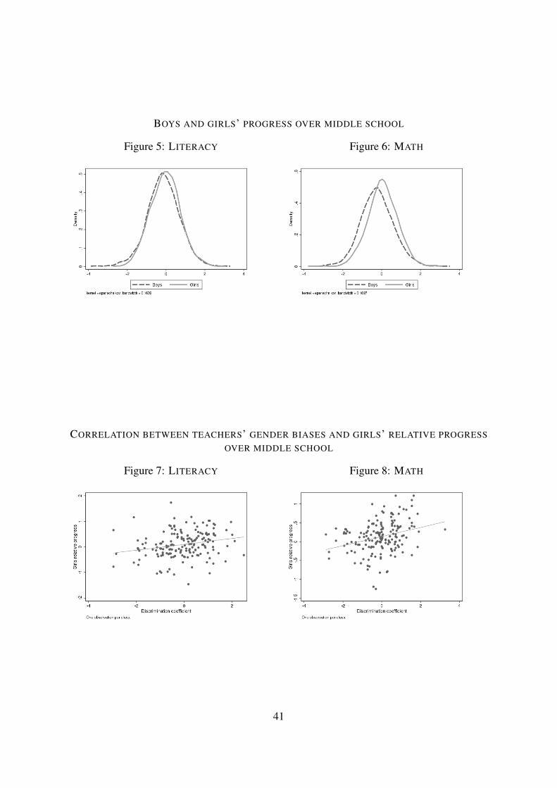
BOYS AND GIRLS’ PROGRESS OVER MIDDLE SCHOOL
Figure 5: LITERACY Figure 6: MATH
CORRELATION BETWEEN TEACHERS’ GENDER BIASES AND GIRLS’ RELATIVE PROGRESS
OVER MIDDLE SCHOOL
Figure 7: LITERACY Figure 8: MATH
41

Table 2: ESTIMATION OF THE GENDER BIAS
Dep var : Math scores (1) (2) (3) (4) (5)
Girl x Non-Blind 0.318*** 0.327*** 0.317*** 0.313*** 0.318***(0.027) (0.031) (0.029) (0.027) (0.031)
Girl -0.152*** -0.146** -0.211*** -0.160*** -0.221***(0.028) (0.040) (0.039) (0.028) (0.039)
Non-Blind Score -0.156** -0.170* -0.147* -0.150** -0.145(0.052) (0.064) (0.067) (0.051) (0.071)
Controls for punishment . .Punishment -0.566*** -0.546***
(0.076) (0.075)Punishment x Non-Blind -0.153* -0.152*
(0.071) (0.070)Punishment x Non-Blind x Girl -0.301 -0.296
(0.157) (0.170)Controls for grade repetition . .Grade repetition -0.352*** -0.383**
(0.090) (0.125)Repetition x Non-Blind -0.076 -0.007
(0.133) (0.096)Repetition x Non-Blind x Girl 0.077 -0.040
(0.112) (0.165)Constant 2.361*** 4.717*** 5.034*** 2.492*** 5.170***
(0.133) (0.062) (0.067) (0.127) (0.072)Class FE Yes Yes Yes Yes YesR2 0.118 0.105 0.136 0.125 0.143Number of observations 8329 4413 4413 8329 4413
Notes: The dependent variable is the score (both blind and non-blind) obtained by a pupil inmath during the first term of grade 6. Each pupil has two observations: one for the blind scoreand one for the non-blind score. The sample used in columns 2, 3, and 5 does not include pupilsfor which a punishment variable is missing. Standard errors are in parentheses and have beenestimated with school-level clusters. Stars correspond to the following p-values: * p<.05; **p<.01; *** p<.001.
42
Table 3: INDEPENDANCE OF TEACHERS’ASSIGNMENT
Math LiteracyDep var: Bias Girls Boys Girls Boys
Blind -0.003 -0.052** 0.019 -0.029(0.020) (0.018) (0.021) (0.020)
High SES 0.044 -0.039 -0.154** 0.004(0.046) (0.047) (0.051) (0.046)
Low SES -0.031 0.038 0.075 0.061(0.038) (0.038) (0.042) (0.039)
Grade repetition -0.092 0.121 -0.196** -0.044(0.071) (0.065) (0.090) (0.071)
† Notes: Stars correspond to the following p-values: * p<.05; **p<.01; *** p<.001. Each cell in this table corresponds to thecoefficient of a separate regression run on the full sample. Forinstance, the upper left cell reports the coefficient of the regres-sion of the bias of math teachers on the blind score of girls inmath.
Table 4:BALANCE CHECK OF ATTRITION AT THE INDIVIDUAL LEVEL
Grade 9 Grade 10 Grade 11
Math Literacy Math Literacy Math LiteracyDep var: % girls missing 0.005 -0.004 -0.002 -0.001 -0.002 -0.001
(0.011) (0.009) (0.011) (0.009) (0.011) (0.009)Dep var: % boys missing 0.001 -0.003 0.001 -0.008 0.001 -0.008
(0.010) (0.009) (0.009) (0.010) (0.009) (0.010)Number of observations 177 172 177 172 177 172† Notes: Stars correspond to the following p-values: * p<.05; ** p<.01; *** p<.001. One obser-
vation per class. In the upper and bottom part of the table, the dependent variable corresponds tothe percentage of girls (respectively boys) with a missing score. In columns 1 and 2, the depen-dent variable is the percentage of girls (respectively boys) for which the blind score is missingat the end of grade 9 (blind score missing in math in column 1 and literature in column 2). Incolumns 3 and 4, the dependent variable is the percentage of girls (respectively boys) for whichthe high school attended from grade 10 is missing. In columns 5 and 6, the dependent variableis the percentage of girls (respectively boys) for which the course choice in grade 11 is missing.Robust standard errors.
43

Table 5: EFFECT OF TEACHERS’ GENDER BIASES ON
GIRLS’ PROGRESS RELATIVE TO BOYS
Math LiteratureDep var : (ProgresG − ProgresB)c
Gender bias 0.136*** 0.129**(0.047) (0.053)
Achievement gap -0.191*** -0.178**(0.069) (0.090)
Constant 0.088*** 0.160***(0.032) (0.046)
Observations 177 172R-Square 0.132 0.079† Notes: The unit of observation is a class. The dependent variable is
the gap between girls’ and boys’ progress between the beginning ofgrade 7 and the end of grade 9. Standard errors are in parentheses andhave been estimated with a two-step bootstrapping method. Starscorrespond to the following p-values: * p<.10; ** p<.05; *** p<.01.
Table 6: EFFECT OF TEACHERS’ GENDER BIASES ON GIRLS’ SCHOOL CHOICE, COURSE CHOICE,AND GRADE REPETITION RELATIVE TO BOYS’
Dep var:(ProbG − ProbB)c General HS Science Literature Repetition
Bias in Bias in Bias in Bias inMath Literacy Math Literacy Math Literacy Math Literacy
Gender bias 0.015 0.007 0.027* 0.013 -0.009 0.005 -0.026 -0.014(0.021) (0.022) (0.016) (0.015) (0.010) (0.011) (0.019) (0.021)
Achievement gap 0.208*** 0.263*** 0.149*** 0.152*** 0.047** 0.047** -0.072** -0.077**(0.034) (0.034) (0.024) (0.025) (0.019) (0.019) (0.029) (0.036)
Constant 0.125*** -0.017 0.022* 0.023* 0.048*** 0.049*** -0.108*** -0.063***(0.017) (0.021) (0.012) (0.013) (0.012) (0.011) (0.015) (0.019)
Observations 177 172 177 172 177 172 177 172R-Square 0.158 0.184 0.173 0.149 0.031 0.031 0.047 0.031† Notes: The unit of observation is a class. In columns 1 and 2, the dependent variable is the gap between girls’ and boys’
probability to choose a general high school from grade 10. In columns 3 and 4, the dependent variable is the gap betweengirls’ and boys’ probability to choose a scientific track in grade 11. In columns 5 and 6, the dependent variable is the gapbetween girls’ and boys’ probability to choose a literature track in grade 11. In columns 7 and 8, the dependent variable isthe gap between girls’ and boys’ probability to repeat a grade. Standard errors are in parentheses and have been estimatedwith a two-step bootstrapping method. Stars correspond to the following p-values: * p<.10; ** p<.05; *** p<.01.
44

Table 7: EFFECT OF TEACHERS’ BIASES WITH SPILLOVERS
Progress over 3 years ScienceDep var: in course(PG − PB)c Math Math Literature Literature
Gender Bias Math 0.136*** 0.135*** 0.067 0.026* 0.025(0.047) (0.047) (0.057) (0.015) (0.016)
Gender Bias Literacy 0.034 0.129** 0.134*** 0.009(0.038) (0.053) (0.046) (0.015)
Achievement Gap -0.191*** -0.209*** -0.178** -0.197** 0.151*** 0.148***(0.069) (0.071) (0.090) (0.089) (0.022) (0.023)
Constant 0.088*** 0.080** 0.160*** 0.177*** 0.026** 0.028**(0.032) (0.032) (0.046) (0.045) (0.012) (0.012)
Observations 177 170 172 170 177 170R-Square 0.132 0.154 0.079 0.108 0.190 0.184† Notes: The unit of observation is a class. In columns 1 to 4, the dependent variable is the gap between
girls’ and boys’ progress between the beginning of grade 7 and the end of grade 9. In columns 5 and 6,the dependent variable is the gap between girls’ and boys’ probability to select a science course in grade11. Standard errors are in parentheses and have been estimated with a two-step bootstrapping method.Stars correspond to the following p-values: * p<.10; ** p<.05; *** p<.01.
Table 8: CUMULATIVE EFFECT OF TEACHERS’ BIASES
Dep var:(ProgresG − ProgresB)c Math Math Literature Literature
Gender Bias 0.136*** 0.142*** 0.129** 0.118*(0.047) (0.051) (0.053) (0.064)
Achievement Gap -0.191*** -0.191*** -0.178** -0.178**(0.069) (0.070) (0.090) (0.090)
Gender Bias*Pct Same Teacher -0.075 0.112(0.270) (0.298)
Observations 177 177 172 172R-Square 0.132 0.133 0.079 0.081† Notes: The unit of observation is a class. In columns 1 to 4, the dependent variable is
the gap between girls’ and boys’ progress between the beginning of grade 7 and the endof grade 9. Standard errors are in parentheses and have been estimated with a two-stepbootstrapping method. Stars correspond to the following p-values: * p<.10; ** p<.05; ***p<.01.
45

BOYS LAG BEHIND.
HOW TEACHERS’ GENDER BIASES AFFECT STUDENTS’ ACHIEVEMENT
Camille Terrier
APPENDIX
A Additional tables
46

Table A.1: SKILLS MEASURED BY STANDARDIZED TESTS AND CLASS EXAMS
Blind score Non-Blind scoreMath
Space and geometry GeometryRecognize and draw two-dimensional figures Two-dimensional figuresProperties of alignment, perpendicular, parallel, and symmetry Symmetry of a straight lineRecognize a cube shape and parallelepiped rectangle Parallelepiped rectangleHow to exploit numerical data Organize and understand dataSolve a problem using proportionality ProportionalitySolve problems with addition/substraction/multiplication/division Read information in tablesRead and interpret a table, diagram, and graphic Read information on axis, diagrams/graphicsSize and measurement Size and measurementKnowledge and use of measurement units Length, mass, and duration(length, mass, volums, and duration) Angles
Area: measure, comparison, and calculusVolumes
Knowledge of natural whole numbers Numbers and calculusKnowledge of integers Integer numbers and decimalsUse and writing of fractions FractionsUse decimal numbersCalculusKnowledge of the four operations Operations
LiteracyKnowledge and recognition of words GrammarUnderstand the formation of words Classes of words (noun, pronoun, verb)Exploit time-space indications ConjugationKnowledge of verb tenses Tenses (present/past/future)
SpellingGrammatical spellingLexical spelling
Understanding of words VocabularyDecipher rare words ReadingUnderstand the meaning of a word with its contextClassify and link informationProduction of a text WritingAdd punctuation to a text Use of punctuationProduce a coherent text Production of a text (one page max)Transform a textUse of usual words
Oral expression (reading aloud, recitation)Initiation to art history
47

B Estimation of Teachers’ Gender Bias with Control Vari-
ables
In this section, I successively check how pupils’ disruptive behavior in the class, having re-
peated a grade, and pupils’ initial achievement affect the gender bias estimate. Taking this into
account is important, as these variables could be correlated to both teachers’ gender bias and a
student’s progress.
Controlling for Pupils’ Disruptive Behavior and Grade Repetition. Boys are more dis-
ruptive than girls (Table 1). If bad behavior influences teachers’ assessments (consciously or
not), this could affect the estimate of the gender bias.29 Based on the extensive information
I have on pupils’ behavior, I create a variable “punishment” that takes a value of 1 if a pupil
has received a disciplinary warning from the class council during the first term of grade 6 or
if he/she was temporarily excluded from the school. It is important to highlight that both pun-
ishments are not given by a single teacher, but by the head teacher in agreement with all the
teachers of a student. From that perspective, punishment is not determined solely by the teach-
ers handing out grades. During the first term of grade 6, 8 percent of pupils—85 percent of
which were boys—received at least one sanction.30 Results including the punishment variable
are presented in Table 2, column 3.31 Regressions are run in math only, where a gender bias
is observed. Column 2 presents results of the standard DiD regression implemented on the
smaller sample of students for which the punishment information is available. The coefficient
29Cornwell et al. (2013), using data from the 1998-1999 ECLS-K cohort of primary school pupils, took intoaccount pupils’ non cognitive skills to explain why "boys who perform equally as well as girls on reading, mathand science tests are graded less favorably by their teachers." More specifically, the authors used teachers’ re-ported information on how well a pupil is "engaged in the classroom" and found that controlling for this variablesignificantly reduces or completely removes the bias in teachers’ grades, depending on pupils’ ethnicity and thegrade considered.
30This gender gap in disruptive behavior is consistent with prior research. In the U.S., by fifth grade, Bertrand,Pan (2013) found that girls score about half a standard deviation below boys in teacher-reported externalizingproblems, which is an important determinant of school suspension.
31Several schools did not provide information on their pupils’ behavior, so that the punishment variable ismissing for some pupils. Therefore, following regressions will focus on the sample of 2269 pupils for whichpunishments are available. Because this sample is different from the full sample, I run a balance check to verifyif pupils’ characteristics differ. No significant differences are found regarding the blind score, non-blind score,gender, and parents’ professions. Even if schools that do not provide information on sanctions are the ones withthe worst-behaved students, my results will be a lower bound of the effect of pupils’ behavior on gender bias.
48

for teachers’ gender biases decreases when I control for pupils’ behavior, but the drop is very
small: the point estimate goes from 0.327 to 0.317. This suggests that the gender bias I observe
in math does not capture boys’ disruptive behavior.32
Grade repetition is another characteristic that might influence teachers’ grades. Like be-
havior, grade repetition is not equally distributed for boys and girls. Among pupils who have
repeated a grade, 62.2 percent are boys. As previously, I include a dummy for grade repetition
in the regression. Results presented in column 4 of Table 2 suggest that grade repetition does
not explain the bias against boys. I also test whether parents’ professions have an impact on
teachers’ gender biases and find no significant effect of pupils’ social backgrounds.
Quantile Regressions. Finally, I test if the bias against boys captures two potentially re-
lated effects: (1) some teachers might give more favorable grades to low achievers, and (2) in
some classes, the variance of teachers’ grades might be smaller than the variance of the stan-
dardized scores. Regarding the first point, some teachers might behave differently toward low
performers and potentially give them higher grades than expected by their ability. If this is the
case, since girls perform worse than boys in math at the beginning of grade 6, the gender bias
estimate could partially capture a positive bias in favor of low achievers. Regarding the second
element, some teachers might have a lower dispersion of their grades than the dispersion of the
standardized scores. For a given dispersion of blind scores in a classroom, reducing the disper-
sion of non-blind scores will improve the non-blind score of the weakest in the class, relative
to the scores of the best pupils. Again, since girls have initially lower scores than boys in math,
a teacher who prefers a reduced dispersion of his grades will advantage girls relative to boys.
To take both effects into account, I run quantile regressions. Results in math are presented
in Table A.2. The 0.5 quantile coefficient for the conditional median equals 0.308, which is
close to the DiD coefficient (0.318). However, the values for the lowest and highest deciles
tend to differ more. The largest gender bias is observed in the lowest decile of the blind scores,
32A variable that controls for pupils’ bad behavior is included, but girls’ behavior might also affect non-blindscores through more diffuse aspects (Cornwell et al. (2013)): how they behave in the classroom, how often theyanswer questions, and the diligence they show in their work. I consider that these elements will not bias the resultsas long as they are a component of my definition of girls. In this case, the coefficient for gender bias capturessome characteristics that are intrinsically linked to girls.
49

Table A.2: QUANTILE REGRESSION COEFFICIENTS FOR THE GENDER BIAS
Quantile DiD
Dep var : B and NB Scores 0.1 0.25 0.5 0.75 0.9 -
Girl x Non-Blind 0.299*** 0.317*** 0.352*** 0.320*** 0.280*** 0.318***(0.075) (0.068) (0.063) (0.062) (0.058) (0.027)
Girls -0.060 -0.112* -0.141** -0.205*** -0.236*** -0.147***(0.043) (0.047) (0.046) (0.048) (0.048) (0.026)
Non-Blind Score -0.230*** -0.134** -0.084 -0.099* -0.198*** -0.155**(0.046) (0.047) (0.045) (0.042) (0.034) (0.052)
Constant -0.578* 0.454 1.368*** 2.203*** 2.676*** 1.255*(0.264) (0.259) (0.208) (0.183) (0.165) (0.463)
Class FE Yes Yes Yes Yes Yes YesR2 0.015Number of observations 8329 8329 8329 8329 8329 8329† Notes: All tests scores are standardized. The dependent variable is the score (both blind and non-blind) obtained
by a pupil in math during the first term of grade 6. Each pupil has two observations: one for the blind scoreand one for the non-blind score. Standard errors are in parentheses and have been estimated with school-levelclusters. Stars correspond to the following p-values: * p<.05; ** p<.01; *** p<.001.
with a coefficient of 0.327. The smallest gender bias is observed in the highest decile of the
distribution, with a coefficient of 0.272. Apart from these two values in the tails of the score
distributions, the gender bias seems reasonably stable across quantiles. As a second test, I
run the regression on pupils’ ranks instead of pupils’ test scores. Teachers’ narrower or larger
dispersions of their grades do not affect their pupils’ rankings within class. Hence, running
DiD regressions with pupils’ ranks as a dependent variable is a mean to control for teachers’
smaller/larger variance of grades. The results are consistent with previous conclusions: the
interaction term equals -2.2 in math, meaning that girls’ average rank decreases by 2.2 when
they are assessed by their teacher.
50

C Estimation of Gender Biases at the End of Grade 6
Table A.3: ESTIMATION OF THE GENDER BIAS - THIRD TERM
(1) (2) (3) (4) (5)Dep var : Math scoresGirl x Non-Blind 0.259*** 0.251*** 0.220*** 0.251*** 0.213***
(0.035) (0.041) (0.042) (0.036) (0.044)Girls -0.045 -0.039 -0.106 -0.053 -0.108
(0.037) (0.051) (0.053) (0.036) (0.053)Non-Blind Score -0.120 -0.182 -0.139 -0.111 -0.132
(0.069) (0.089) (0.089) (0.067) (0.088)Controls for punishment . .Punishment -0.700*** -0.683***
(0.050) (0.052)Punishment x Non-Blind -0.168** -0.163**
(0.045) (0.043)Punishment x Non-Blind x Girl 0.036 0.031
(0.098) (0.095)Controls for grade repetition . .Grade repetition -0.372*** -0.297**
(0.074) (0.084)Repetition x Non-Blind -0.119 -0.114
(0.144) (0.193)Repetition x Non-Blind x Girl 0.132 0.126
(0.132) (0.166)Constant -1.398*** 2.220*** 1.672*** -1.384*** 1.737***
(0.066) (0.125) (0.125) (0.065) (0.123)Class FE Yes Yes Yes Yes YesR2 0.122 0.126 0.181 0.131 0.188Number of observations 7714 4460 4460 7714 4460
Notes: The dependent variable is the score (both blind and non-blind) obtained by a pupil inmath during third term. The full sample is used in columns 1 and 4. The sample used in columns2, 3, and 5 does not include pupils for which a punishment variable is missing. Standard errorsare in parentheses and have been estimated with school-level clusters. Stars correspond to thefollowing p-values: * p<.10; ** p<.05; *** p<.01.
51
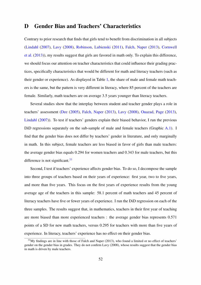
D Gender Bias and Teachers’ Characteristics
Contrary to prior research that finds that girls tend to benefit from discrimination in all subjects
(Lindahl (2007), Lavy (2008), Robinson, Lubienski (2011), Falch, Naper (2013), Cornwell
et al. (2013)), my results suggest that girls are favored in math only. To explain this difference,
we should focus our attention on teacher characteristics that could influence their grading prac-
tices, specifically characteristics that would be different for math and literacy teachers (such as
their gender or experience). As displayed in Table 1, the share of male and female math teach-
ers is the same, but the pattern is very different in literacy, where 85 percent of the teachers are
female. Similarly, math teachers are on average 3.5 years younger than literacy teachers.
Several studies show that the interplay between student and teacher gender plays a role in
teachers’ assessment (Dee (2005), Falch, Naper (2013), Lavy (2008), Ouazad, Page (2013),
Lindahl (2007)). To test if teachers’ genders explain their biased behavior, I run the previous
DiD regressions separately on the sub-sample of male and female teachers (Graphic A.1). I
find that the gender bias does not differ by teachers’ gender in literature, and only marginally
in math. In this subject, female teachers are less biased in favor of girls than male teachers:
the average gender bias equals 0.294 for women teachers and 0.343 for male teachers, but this
difference is not significant.33
Second, I test if teachers’ experience affects gender bias. To do so, I decompose the sample
into three groups of teachers based on their years of experience: first year, two to five years,
and more than five years. This focus on the first years of experience results from the young
average age of the teachers in this sample: 58.1 percent of math teachers and 45 percent of
literacy teachers have five or fewer years of experience. I run the DiD regression on each of the
three samples. The results suggest that, in mathematics, teachers in their first year of teaching
are more biased than more experienced teachers : the average gender bias represents 0.571
points of a SD for new math teachers, versus 0.295 for teachers with more than five years of
experience. In literacy, teachers’ experience has no effect on their gender bias.
33My findings are in line with those of Falch and Naper (2013), who found a limited or no effect of teachers’gender on the gender bias in grades. They do not confirm Lavy (2008), whose results suggest that the gender biasin math is driven by male teachers.
52

Figure A.1: GENDER BIAS COEFFICIENT BY TEACHERS’ GENDERS AND YEARS OF
EXPERIENCE
E Within-Gender between-Subjects Estimation
The following equation is used to obtain the within-gender between-subject estimate of the
gender bias:
Scoins = α0+α1Gi+α2NBi+α3Si+α4Gi∗NBi+α5Gi∗Si+α6NBi∗Si+α7Gi∗NBi∗Si+πc+εins
(16)
Here, Scoins is the grade received by a pupil when the nature of scoring is n (n=1 for non-
blind and 0 for blind) and the subject is s (s=1 for math and 0 for literacy). Hence, for each
pupil i, this dependent variable is a vector of both blind and non-blind grades received in math
and literacy. Si corresponds to a dummy equal to 1 when the grade is given in math (0 in
literacy). α7 is the parameter of interest: the change in the gender bias when the grade is in
math rather than in literacy. Introducing the triple-interaction term Gi ∗ NBi ∗ Si implies that
α7 is estimated using only within-gender and between-subject differences. The key advantage
of this identification is that it allows girls and boys to have different unobserved characteris-
tics (response to stakes and competitiveness, behavior, etc.). α7 is identified as long as these
differences do not vary across subjects. In other words, the potential correlation between the
error term εins and the gender bias Gi ∗ NBi is not problematic as long as the error term is
53

independent from the difference in gender bias between subjects—the triple-interaction term.
Results are presented below and commented on directly in the paper.
Table A.4: ESTIMATION OF THE
GENDER BIAS USING TRIPLE
DIFFERENCES
Girls x Non-Blind x Math 0.291***(0.037)
Girls 0.426***(0.019)
Math 0.281***(0.027)
Non-Blind Score -0.010(0.044)
Girls x Non-Blind 0.027(0.032)
Girls x Math -0.580***(0.019)
Non-Blind x Math -0.146**(0.047)
Constant 1.470***(0.151)
Class FE YesR2 0.116Number of observations 16644
Notes: The dependent variable is thescore, both blind and non-blind, obtainedby a pupil in math and in literacy. Stan-dard errors are in parentheses and havebeen estimated with school-level clus-ters. Stars correspond to the following p-values: * p<.05; ** p<.01; *** p<.001.
F Correlation between the Skills Measured by the Blind and
the Non-Blind Scores
In mathematical terms, the assumption that both tests measure the same ability is equivalent to
ρ = 1 and vi = 0 in Equation 14 defined in section VI.A: θ2i = ρθ1i + vi. If we relax this
54

hypothesis, we are back to the reduced-form equation presented previously:
NBi = α0 + ρBi + α2Gi + (εiNB + vi − ρεiB)
A way to test the validity of the hypothesis is to directly estimate the reduced-form equation
above and to verify if the coefficient ρ is significantly different from 1. If not, both tests can be
assumed to measure abilities that are very similar, and DiD estimates can safely be assumed to
be unbiased.34 However, to correctly estimate the parameter ρ in this equation, I have to get rid
of the measurement error bias. Since Bi is a noisy measure of ability θ1i, it is correlated to the
measurement error εiB. I solve this endogeneity issue by instrumenting Bi. A pupil’s month of
birth is used as an instrument that is correlated to his/her blind score but is independent from
the error term.
In the literature, students’ months of birth have been shown to be an important determinant
of pupils’ success at school (Angrist, Krueger (1991), Bedard, Dhuey (2006), Crawford et al.
(2007)). I test the correlation between blind scores and pupils’ months of birth by running a
regression of blind scores in literacy and math on a set of 11 dummies for each month of birth.
January is taken as the reference month so that all coefficients should be interpreted relatively
to this month. Figure A.2 presents the correlation coefficients.
34I will discuss in a further section an additional assumption required for the DiD to be unbiased. Although wecannot test whether vi = 0, the term vi should be equally distributed between boys and girls.
55
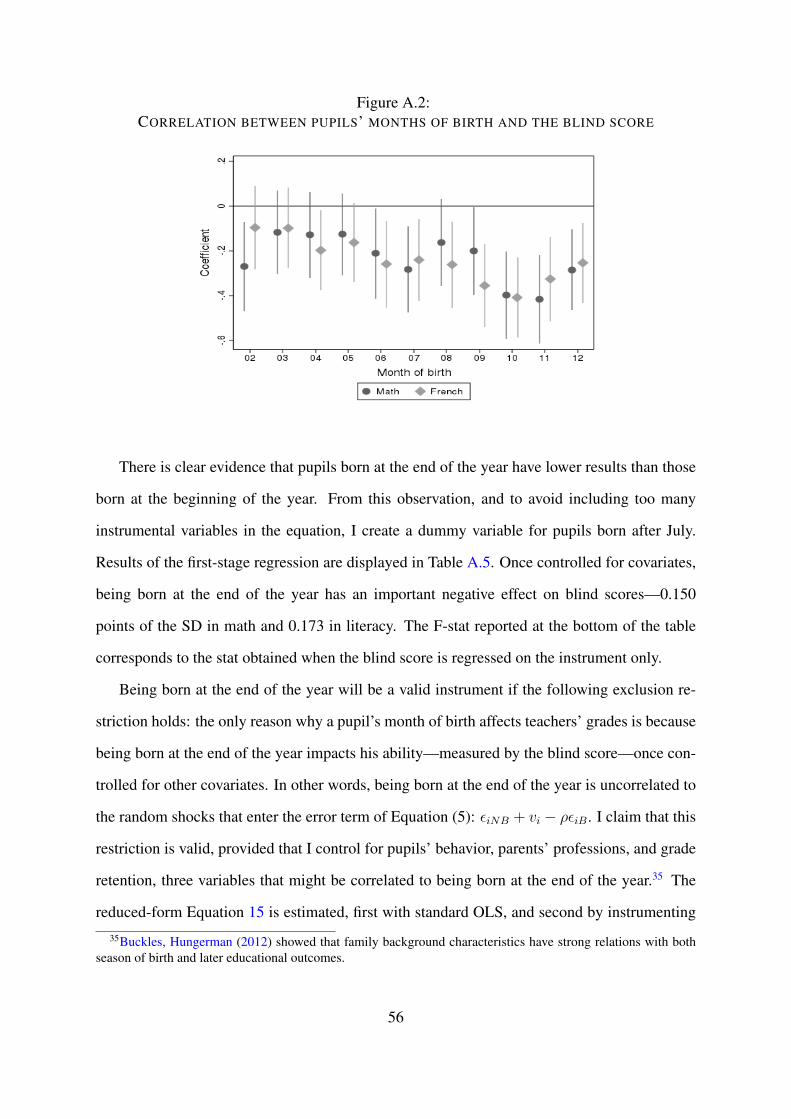
Figure A.2:CORRELATION BETWEEN PUPILS’ MONTHS OF BIRTH AND THE BLIND SCORE
There is clear evidence that pupils born at the end of the year have lower results than those
born at the beginning of the year. From this observation, and to avoid including too many
instrumental variables in the equation, I create a dummy variable for pupils born after July.
Results of the first-stage regression are displayed in Table A.5. Once controlled for covariates,
being born at the end of the year has an important negative effect on blind scores—0.150
points of the SD in math and 0.173 in literacy. The F-stat reported at the bottom of the table
corresponds to the stat obtained when the blind score is regressed on the instrument only.
Being born at the end of the year will be a valid instrument if the following exclusion re-
striction holds: the only reason why a pupil’s month of birth affects teachers’ grades is because
being born at the end of the year impacts his ability—measured by the blind score—once con-
trolled for other covariates. In other words, being born at the end of the year is uncorrelated to
the random shocks that enter the error term of Equation (5): εiNB + vi − ρεiB. I claim that this
restriction is valid, provided that I control for pupils’ behavior, parents’ professions, and grade
retention, three variables that might be correlated to being born at the end of the year.35 The
reduced-form Equation 15 is estimated, first with standard OLS, and second by instrumenting
35Buckles, Hungerman (2012) showed that family background characteristics have strong relations with bothseason of birth and later educational outcomes.
56
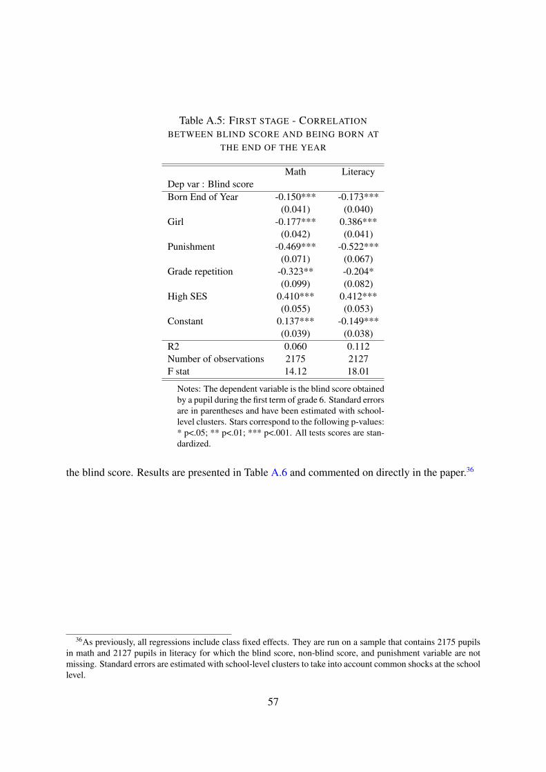
Table A.5: FIRST STAGE - CORRELATION
BETWEEN BLIND SCORE AND BEING BORN AT
THE END OF THE YEAR
Math LiteracyDep var : Blind scoreBorn End of Year -0.150*** -0.173***
(0.041) (0.040)Girl -0.177*** 0.386***
(0.042) (0.041)Punishment -0.469*** -0.522***
(0.071) (0.067)Grade repetition -0.323** -0.204*
(0.099) (0.082)High SES 0.410*** 0.412***
(0.055) (0.053)Constant 0.137*** -0.149***
(0.039) (0.038)R2 0.060 0.112Number of observations 2175 2127F stat 14.12 18.01
Notes: The dependent variable is the blind score obtainedby a pupil during the first term of grade 6. Standard errorsare in parentheses and have been estimated with school-level clusters. Stars correspond to the following p-values:* p<.05; ** p<.01; *** p<.001. All tests scores are stan-dardized.
the blind score. Results are presented in Table A.6 and commented on directly in the paper.36
36As previously, all regressions include class fixed effects. They are run on a sample that contains 2175 pupilsin math and 2127 pupils in literacy for which the blind score, non-blind score, and punishment variable are notmissing. Standard errors are estimated with school-level clusters to take into account common shocks at the schoollevel.
57

Table A.6:OLS AND IV ESTIMATES OF THE REDUCED FORM
OLS IV
Math Literacy Math LiteracyDep var : Non-Blind scoreBlind score 0.760*** 0.684*** 1.090*** 0.964***
(0.019) (0.031) (0.100) (0.099)Girl 0.264*** 0.172*** 0.339*** 0.080
(0.028) (0.043) (0.032) (0.057)Constant -4.794*** -9.031*** -7.617*** -11.585***
(0.190) (0.309) (0.846) (0.896)Class FE Yes Yes Yes YesControls Yes Yes Yes YesR2 0.687 0.607 0.594 0.549Number of observations 2175 2127 2175 2127p-val(Blind=1) 0.37 0.72
Notes: Standard errors are in parentheses and have been estimated with school-levelclusters. Stars correspond to the following p-values : * p<.05; ** p<.01; *** p<.001.The unit of observation is a pupil. The sample contains 2175 pupils in math and 2127pupils in literacy for which the blind score, non-blind score, and punishment variableare not missing. The instrument is a dummy variable equal to 1 if a pupil is bornbetween July and December. Control variables included: grade repetition, punishment,and high SES.
Finally, regarding the exclusion restriction, some might argue that, once controlled for the
abilities measured by the blind score, being born at the end of the year is not perfectly inde-
pendent from unobserved specific skills vi tested by the non-blind score only. If this is the
case, it is likely that being born at the end of the year would also be negatively correlated with
these unobserved skills. Therefore, the IV estimates of ρ might be an upper bound for the true
value of ρ, while the OLS would be a lower bound (due to the downward measurement error
bias). Indeed, the IV estimate is ρIV = Cov(NBi,EndY eari)Cov(Bi,EndY eari)
. If a correlation exists between vi and
being born at the end of the year, this would affect the numerator of the formula by increasing
Cov(NBi, EndY eari). Hence ρIV would be an upper bound for the parameter ρ.
58