77763636 Boyce e Diprima Equacoes Diferencias Elementares 9ª Ed
Upload
jason-hicksCategory
view
233download
5
Boyce/DiPrima 9th ed, Ch 8.5: More on Errors; StabilityElementary Differential Equations and Boundary Value Problems, 9th edition, by William E. Boyce and Richard C. DiPrima, ©2009 by John Wiley & Sons, Inc.
In Section 8.1 we discussed some ideas related to the errors that can occur in a numerical approximation to the solution of the initial value problem y' = f (t, y), y(t0) = y0.
In this section we continue that discussion and also point out some other difficulties that can arise.
Some of the points are difficult to treat in detail, so we will illustrate them by means of examples.
Truncation and Round-off Errors
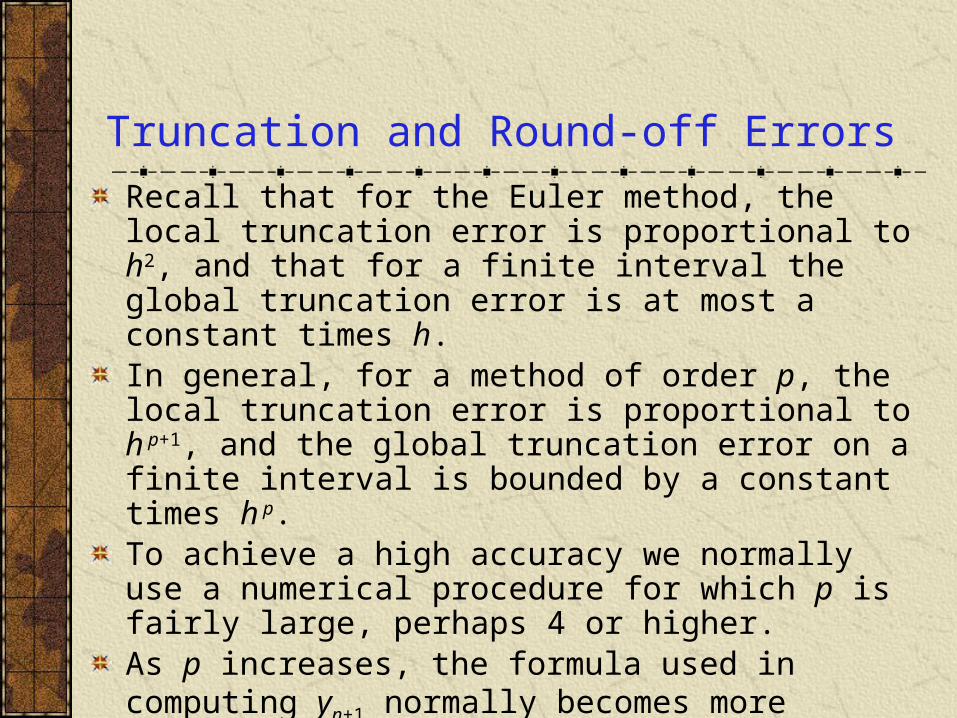
Recall that for the Euler method, the local truncation error is proportional to h2, and that for a finite interval the global truncation error is at most a constant times h. In general, for a method of order p, the local truncation error is proportional to h
p+1, and the global truncation error on a finite interval is bounded by a constant times h
p. To achieve a high accuracy we normally use a numerical procedure for which p is fairly large, perhaps 4 or higher.
As p increases, the formula used in computing yn+1 normally becomes more complicated, and more calculations are required at each step. This is usually not a serious problem unless f (t, y) is complicated, or if the calculation must be repeated many times.
Truncation and Round-off Errors
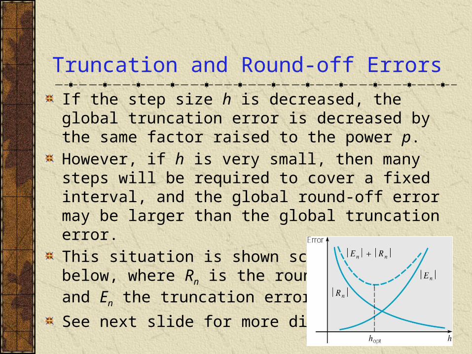
If the step size h is decreased, the global truncation error is decreased by the same factor raised to the power p.
However, if h is very small, then many steps will be required to cover a fixed interval, and the global round-off error may be larger than the global truncation error.
This situation is shown schematically below, where Rn is the round-off error, and En the truncation error, at step n.
See next slide for more discussion.
Truncation and Round-off Errors
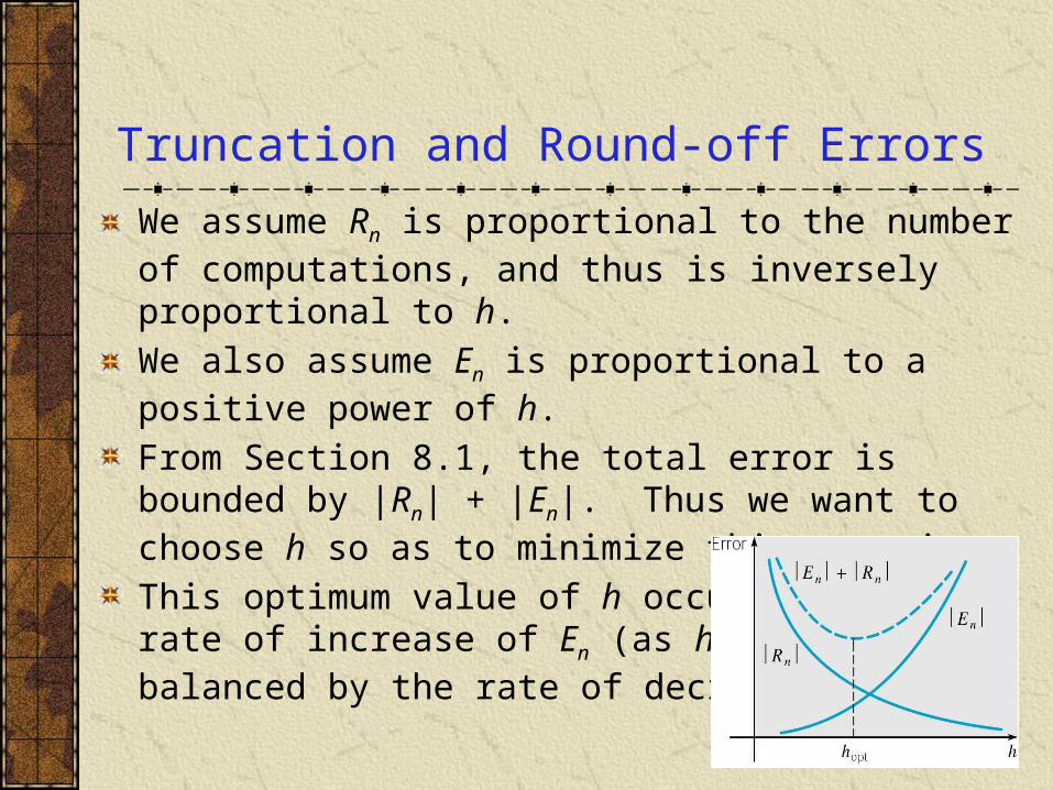
We assume Rn is proportional to the number of computations, and thus is inversely proportional to h.
We also assume En is proportional to a positive power of h.
From Section 8.1, the total error is bounded by |Rn| + |En|. Thus we want to choose h so as to minimize this quantity.
This optimum value of h occurs when the rate of increase of En (as h increases) is balanced by the rate of decrease of Rn.
Example 1: Euler Method Results (1 of 4)
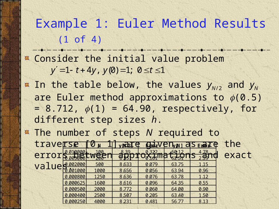
Consider the initial value problem
In the table below, the values yN/2 and yN are Euler method approximations to (0.5) = 8.712, (1) = 64.90, respectively, for different step sizes h.
The number of steps N required to traverse [0, 1] are given, as are the errors between approximations and exact values.
10;1)0(,41 tyyty
h N y[N/2] Error y[N] Error0.010000 100 8.39 0.322 60.12 4.780.005000 200 8.551 0.161 62.51 2.390.002000 500 8.633 0.079 63.75 1.150.001000 1000 8.656 0.056 63.94 0.960.000800 1250 8.636 0.076 63.78 1.120.000625 1600 8.616 0.096 64.35 0.550.000500 2000 8.772 0.060 64.00 0.900.000400 2500 8.507 0.205 63.40 1.500.000250 4000 8.231 0.481 56.77 8.13
Example 1: Error and Step Size (2 of 4)
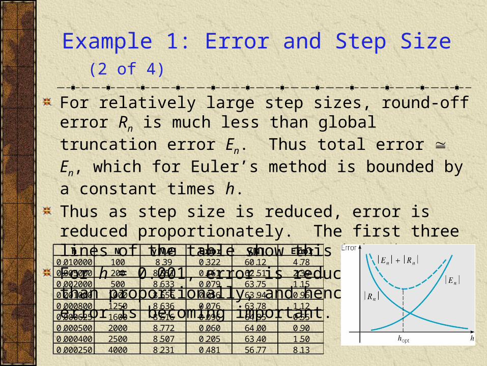
For relatively large step sizes, round-off error Rn is much less than global truncation error En. Thus total error En, which for Euler’s method is bounded by a constant times h.
Thus as step size is reduced, error is reduced proportionately. The first three lines of the table show this behavior.
For h = 0.001, error is reduced, but less than proportionally, and hence round-off error is becoming important.
h N y[N/2] Error y[N] Error0.010000 100 8.39 0.322 60.12 4.780.005000 200 8.551 0.161 62.51 2.390.002000 500 8.633 0.079 63.75 1.150.001000 1000 8.656 0.056 63.94 0.960.000800 1250 8.636 0.076 63.78 1.120.000625 1600 8.616 0.096 64.35 0.550.000500 2000 8.772 0.060 64.00 0.900.000400 2500 8.507 0.205 63.40 1.500.000250 4000 8.231 0.481 56.77 8.13
Example 1: Optimal Step Size (3 of 4)
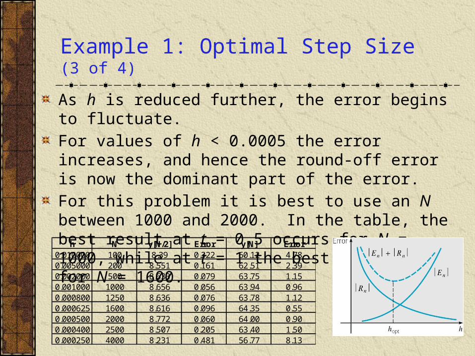
As h is reduced further, the error begins to fluctuate.
For values of h < 0.0005 the error increases, and hence the round-off error is now the dominant part of the error.
For this problem it is best to use an N between 1000 and 2000. In the table, the best result at t = 0.5 occurs for N = 1000, while at t = 1 the best result is for N = 1600.
h N y[N/2] Error y[N] Error0.010000 100 8.39 0.322 60.12 4.780.005000 200 8.551 0.161 62.51 2.390.002000 500 8.633 0.079 63.75 1.150.001000 1000 8.656 0.056 63.94 0.960.000800 1250 8.636 0.076 63.78 1.120.000625 1600 8.616 0.096 64.35 0.550.000500 2000 8.772 0.060 64.00 0.900.000400 2500 8.507 0.205 63.40 1.500.000250 4000 8.231 0.481 56.77 8.13
Example 1: Truncation and Round-Off Error Discussion (4 of 4)
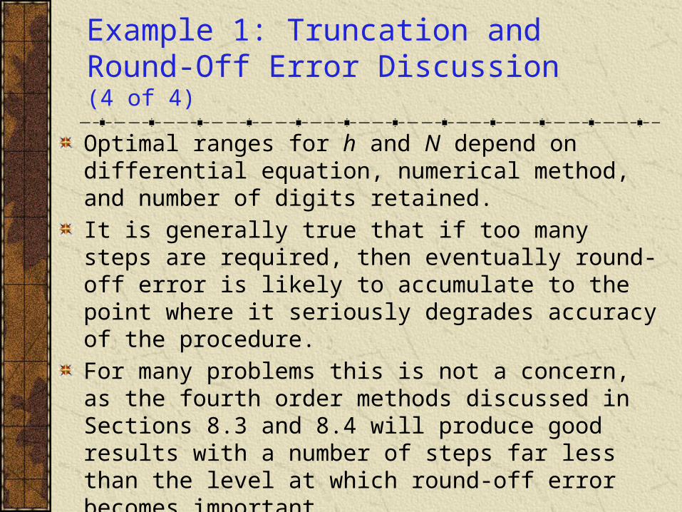
Optimal ranges for h and N depend on differential equation, numerical method, and number of digits retained.
It is generally true that if too many steps are required, then eventually round-off error is likely to accumulate to the point where it seriously degrades accuracy of the procedure.
For many problems this is not a concern, as the fourth order methods discussed in Sections 8.3 and 8.4 will produce good results with a number of steps far less than the level at which round-off error becomes important.
For some problems round-off error becomes vitally important, and the choice of method may become crucial, and adaptive methods advantageous.
Example (Vertical Asymptote):Euler’s Method (1 of 5)
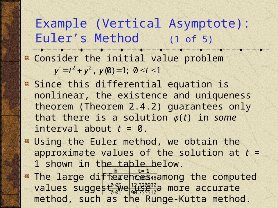
Consider the initial value problem
Since this differential equation is nonlinear, the existence and uniqueness theorem (Theorem 2.4.2) guarantees only that there is a solution (t) in some interval about t = 0.
Using the Euler method, we obtain the approximate values of the solution at t = 1 shown in the table below.
The large differences among the computed values suggest we use a more accurate method, such as the Runge-Kutta method.
10;1)0(,22 tyyty
h t = 10.10 7.1895480.05 12.3209300.01 90.755510
Example (Vertical Asymptote): Runge-Kutta Method (2 of 5)
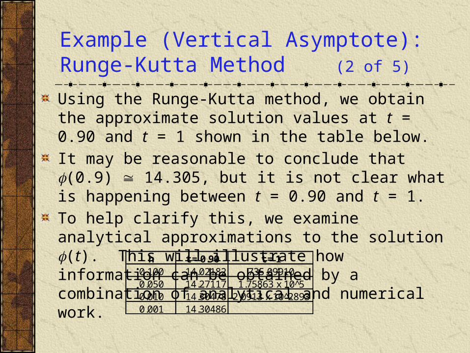
Using the Runge-Kutta method, we obtain the approximate solution values at t = 0.90 and t = 1 shown in the table below.
It may be reasonable to conclude that (0.9) 14.305, but it is not clear what is happening between t = 0.90 and t = 1.
To help clarify this, we examine analytical approximations to the solution (t). This will illustrate how information can be obtained by a combination of analytical and numerical work.
h t = 0.90 t = 10.100 14.02182 735.099100.050 14.27117 1.75863 x 10^50.010 14.30478 2.0913 x 10^28930.001 14.30486
Example (Vertical Asymptote): Analytical Bounds (3 of 5)
Recall our initial value problem
and its solution (t). Note that
It follows that the solution 1(t) of
is an upper bound for (t), and the solution 2(t) of
is an lower bound for (t). That is,
as long as the solutions exist.
10;1)0(,22 tyyty
.10for,1 2222 tyyty
1)0(,1 2 yyy
1)0(,2 yyy
),()()( 12 ttt
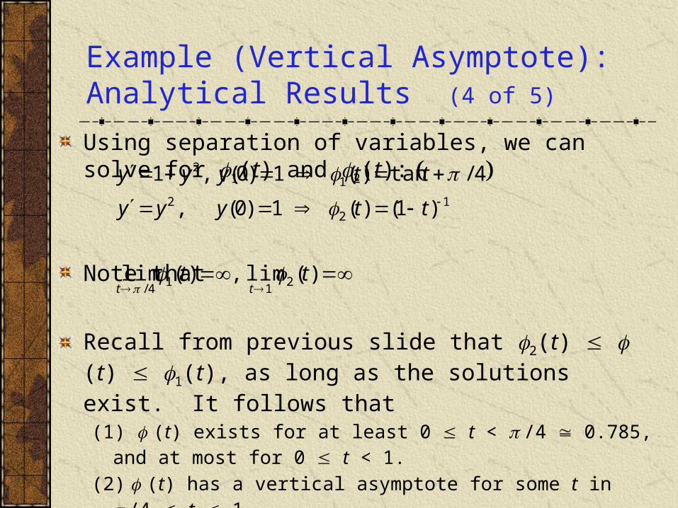
Example (Vertical Asymptote): Analytical Results (4 of 5)
Using separation of variables, we can solve for 1(t) and 2(t):
Note that
Recall from previous slide that 2(t) (t) 1(t), as long as the solutions exist. It follows that(1) (t) exists for at least 0 t < /4 0.785, and at most for 0 t < 1.
(2) (t) has a vertical asymptote for some t in /4 t 1.
Our numerical results suggest that we can go beyond t = /4, and probably beyond t = 0.9.
1
22
12
)1()(1)0(,
4/tan)(1)0(,1
ttyyy
ttyyy
)(lim,)(lim 21
14/
tttt
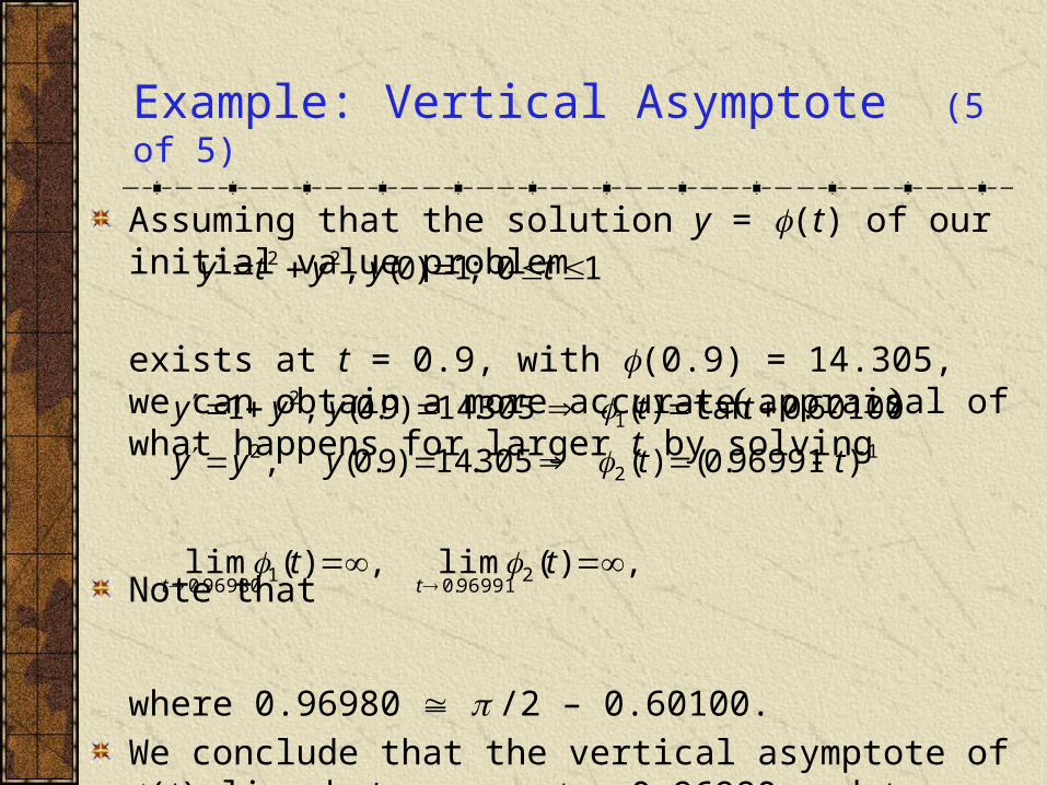
Example: Vertical Asymptote (5 of 5)
Assuming that the solution y = (t) of our initial value problem
exists at t = 0.9, with (0.9) = 14.305, we can obtain a more accurate appraisal of what happens for larger t by solving
Note that
where 0.96980 /2 – 0.60100.
We conclude that the vertical asymptote of (t) lies between t = 0.96980 and t = 0.96991.
10;1)0(,22 tyyty
1
22
12
)96991.0()(305.14)9.0(,
60100.0tan)(305.14)9.0(,1
ttyyy
ttyyy
,)(lim,)(lim 296991.0
196980.0
tttt
Stability (1 of 2)
Stability refers to the possibility that small errors introduced in a procedure die out as the procedure continues. Instability occurs if small errors tend to increase.In Section 2.5 we identified equilibrium solutions as (asymptotically) stable or unstable, depending on whether solutions that were initially near the equilibrium solution tended to approach it or depart from it as t increased. More generally, the solution of an initial value problem is asymptotically stable if initially nearby solutions tend to approach the solution, and unstable if they depart from it. Visually, in an asymptotically stable problem, the graphs of solutions will come together, while in an unstable problem they will separate.
Stability (2 of 2)
When solving an initial value problem numerically, it will at best mimic the actual solution behavior. We cannot make an unstable problem a stable one by solving it numerically.
However, a numerical procedure can introduce instabilities that are not part of the original problem. This can cause trouble in approximating the solution.
Avoidance of such instabilities may require restrictions on the step size h.
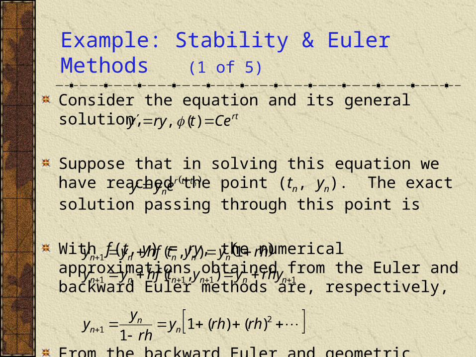
Example: Stability & Euler Methods (1 of 5)
Consider the equation and its general solution,
Suppose that in solving this equation we have reached the point (tn, yn). The exact solution passing through this point is
With f (t, y) = ry, the numerical approximations obtained from the Euler and backward Euler methods are, respectively,
From the backward Euler and geometric series formulas,
rtCetryy )(,
nttrneyy
1111
1
),(
1),(
nnnnnn
nnnnn
rhyyythfyy
rhyythfyy
2
1 )()(11
rhrhyrh
yy n
nn
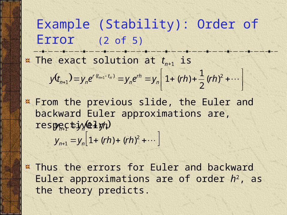
Example (Stability): Order of Error (2 of 5)
The exact solution at tn+1 is
From the previous slide, the Euler and backward Euler approximations are, respectively,
Thus the errors for Euler and backward Euler approximations are of order h2, as the theory predicts.
21
1
)()(1
1
rhrhyy
rhyy
nn
nn
2)(
1 )(2
1)(11 rhrhyeyeyty n
rhn
ttrnn
nn
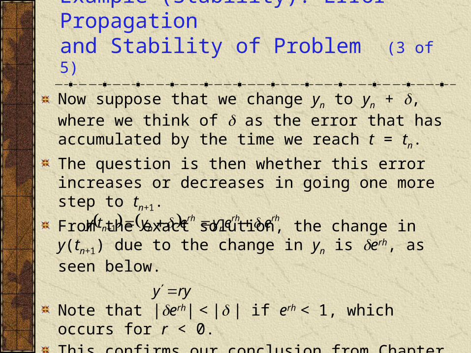
Example (Stability): Error Propagation and Stability of Problem (3 of 5)
Now suppose that we change yn to yn + , where we think of as the error that has accumulated by the time we reach t = tn.
The question is then whether this error increases or decreases in going one more step to tn+1.
From the exact solution, the change in y(tn+1) due to the change in yn is erh, as seen below.
Note that |erh| < | | if erh < 1, which occurs for r < 0.
This confirms our conclusion from Chapter 2 that the equation
is asymptotically stable if r < 0, and is unstable if r > 0.
rhrhn
rhnn eeyeyty 1
ryy
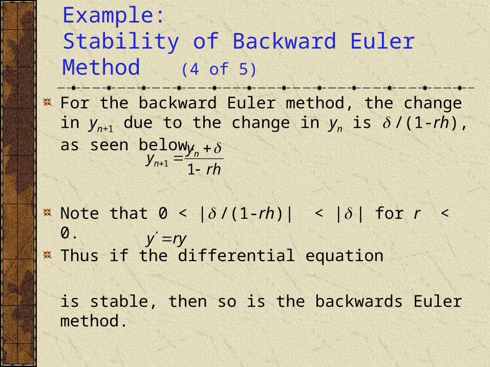
Example: Stability of Backward Euler Method (4 of 5)
For the backward Euler method, the change in yn+1 due to the change in yn is /(1-rh), as seen below.
Note that 0 < | /(1-rh)| < | | for r < 0.
Thus if the differential equation
is stable, then so is the backwards Euler method.
ryy
rh
yy n
n
11
Example: Stability of Euler Method (5 of 5)
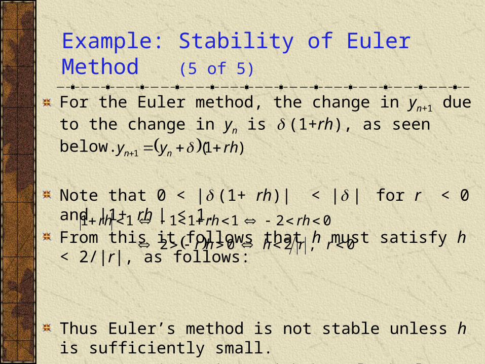
For the Euler method, the change in yn+1 due to the change in yn is (1+rh), as seen below.
Note that 0 < | (1+ rh)| < | | for r < 0 and |1+ rh | < 1.
From this it follows that h must satisfy h < 2/|r|, as follows:
Thus Euler’s method is not stable unless h is sufficiently small.
Note: Requiring h < 2/|r| is relatively mild, unless r is large.
0,202
0211111
rrhhr
rhrhrh
)1(1 rhyy nn
Stiff Problems
The previous example illustrates that it may be necessary to restrict h in order to achieve stability in the numerical method, even though the problem itself is stable for all values of h.
Problems for which a much smaller step size is needed for stability than for accuracy are called stiff.
The backward differentiation formulas of Section 8.4 are popular methods for solving stiff problems, and the backward Euler method is the lowest order example of such methods.
Example 2: Stiff Problem (1 of 4)
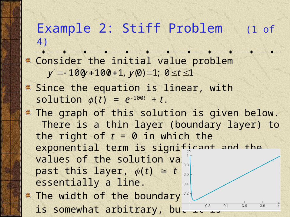
Consider the initial value problem
Since the equation is linear, with solution (t) = e-100t + t.
The graph of this solution is given below. There is a thin layer (boundary layer) to the right of t = 0 in which the exponential term is significant and the values of the solution vary rapidly. Once past this layer, (t) t and the graph is essentially a line.
The width of the boundary layer
is somewhat arbitrary, but it is
certainly small. For example,
at t = 0.1, e-100t 0.000045.
10;1)0(,1100100 tytyy
Example 4: Error Analysis (2 of 4)
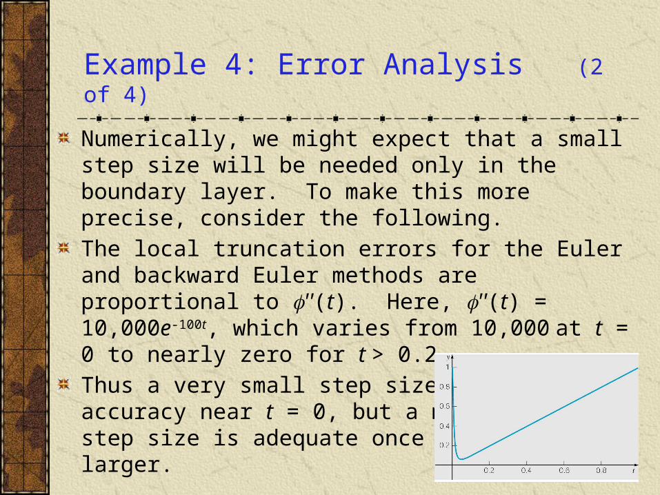
Numerically, we might expect that a small step size will be needed only in the boundary layer. To make this more precise, consider the following.
The local truncation errors for the Euler and backward Euler methods are proportional to ''(t). Here, ''(t) = 10,000e-100t, which varies from 10,000 at t = 0 to nearly zero for t > 0.2.
Thus a very small step size is needed for accuracy near t = 0, but a much larger step size is adequate once t is a little larger.
Example 4: Stability Analysis (3 of 4)
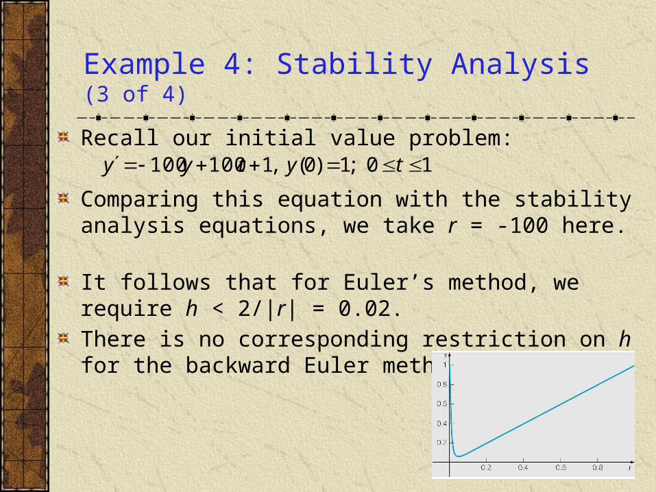
Recall our initial value problem:
Comparing this equation with the stability analysis equations, we take r = -100 here.
It follows that for Euler’s method, we require h < 2/|r| = 0.02.
There is no corresponding restriction on h for the backward Euler method.
10;1)0(,1100100 tytyy
Example 4: Numerical Results (4 of 4)
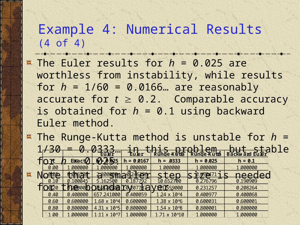
The Euler results for h = 0.025 are worthless from instability, while results for h = 1/60 = 0.0166… are reasonably accurate for t 0.2. Comparable accuracy is obtained for h = 0.1 using backward Euler method.
The Runge-Kutta method is unstable for h = 1/30 = 0.0333… in this problem, but stable for h = 0.025.
Note that a smaller step size is needed for the boundary layer.Euler Euler Runge-Kutta Runge-Kutta Backward Euler
t Exact h = 0.025 h = 0.0167 h = .0333 h = 0.025 h = 0.10.00 1.000000 1.000000 1.000000 1.000000 1.000000 1.0000000.05 0.056738 2.300000 -0.246296 0.4704710.10 0.100045 5.162500 0.187792 10.652700 0.276796 0.1909090.20 0.200000 25.828900 0.207707 111.559000 0.231257 0.2082640.40 0.400000 657.241000 0.400059 1.24 x 10^4 0.400977 0.4000680.60 0.600000 1.68 x 10^4 0.600000 1.38 x 10^6 0.600031 0.6000010.80 0.800000 4.31 x 10^5 0.800000 1.54 x 10^8 0.800001 0.8000001.00 1.000000 1.11 x 10^7 1.000000 1.71 x 10^10 1.000000 1.000000
Example (Numerical Dependence): First Set of Solutions (1 of 6)
Consider the second order equation
Two linearly independent solutions are
where 1(t) and 2(t) satisfy the respective initial conditions
Recall that
It follows that for large t, 1(t) 2(t).
0,010 2 tyy
tttt 10sinh)(,10cosh)( 21
10)0(,0)0(;0)0(,1)0( 2211
2
sin,2
coshtttt ee
tee
t
Example (Numerical Dependence): Numerical Dependence (2 of 6)
Our two linearly independent solutions are
For large t, 1(t) 2(t), and hence these two solutions will look the same if only a fixed number of digits are retained.
For example, at t = 1 and using 8 significant figures, we have
If the calculations are performed on an eight digit machine, the two solutions will be identical on t 1. Thus even though the solutions are linearly independent, their numerical tabulation would be the same.
This phenomenon is called numerical dependence.
tttt 10sinh)(,10cosh)( 21
894.315,1010sinh10cosh
Example (Numerical Dependence): Second Set of Solutions (3 of 6)
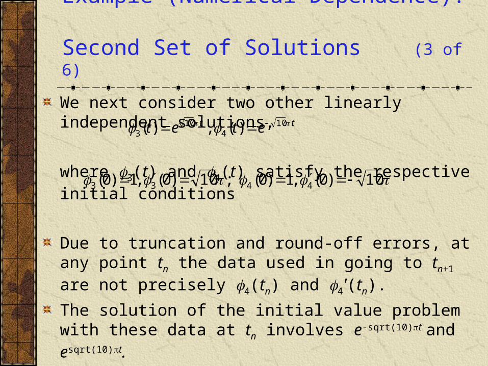
We next consider two other linearly independent solutions,
where 3(t) and 4(t) satisfy the respective initial conditions
Due to truncation and round-off errors, at any point tn the data used in going to tn+1 are not precisely 4(tn) and 4'(tn).
The solution of the initial value problem with these data at tn involves e-sqrt(10)t and esqrt(10)t.
Because the error at tn is small, esqrt(10)t appears with a small coefficient, but nevertheless will eventually dominate, and the calculated solution will be a multiple of 3(t).
tt etet 104
103 )(,)(
10)0(,1)0(;10)0(,1)0( 4433
Example (Numerical Dependence): Runge-Kutta Method (4 of 6)
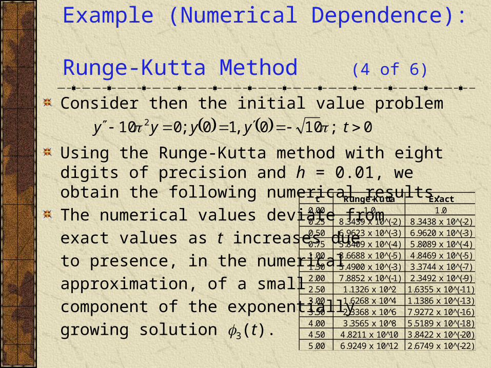
Consider then the initial value problem
Using the Runge-Kutta method with eight digits of precision and h = 0.01, we obtain the following numerical results.
The numerical values deviate from
exact values as t increases due
to presence, in the numerical
approximation, of a small
component of the exponentially
growing solution 3(t).
0;100,10;010 2 tyyyy
t Runge-Kutta Exact0.00 1.0 1.00.25 8.3439 x 10 (̂-2) 8.3438 x 10 (̂-2)0.50 6.9623 x 10 (̂-3) 6.9620 x 10 (̂-3)0.75 5.8409 x 10 (̂-4) 5.8089 x 10 (̂-4)1.00 8.6688 x 10 (̂-5) 4.8469 x 10 (̂-5)1.50 5.4900 x 10 (̂-3) 3.3744 x 10 (̂-7)2.00 7.8852 x 10 (̂-1) 2.3492 x 10 (̂-9)2.50 1.1326 x 10^2 1.6355 x 10 (̂-11)3.00 1.6268 x 10^4 1.1386 x 10 (̂-13)3.50 2.3368 x 10^6 7.9272 x 10 (̂-16)4.00 3.3565 x 10^8 5.5189 x 10 (̂-18)4.50 4.8211 x 10^10 3.8422 x 10 (̂-20)5.00 6.9249 x 10^12 2.6749 x 10 (̂-22)
Example (Numerical Dependence): Round-Off Error (4 of 6)
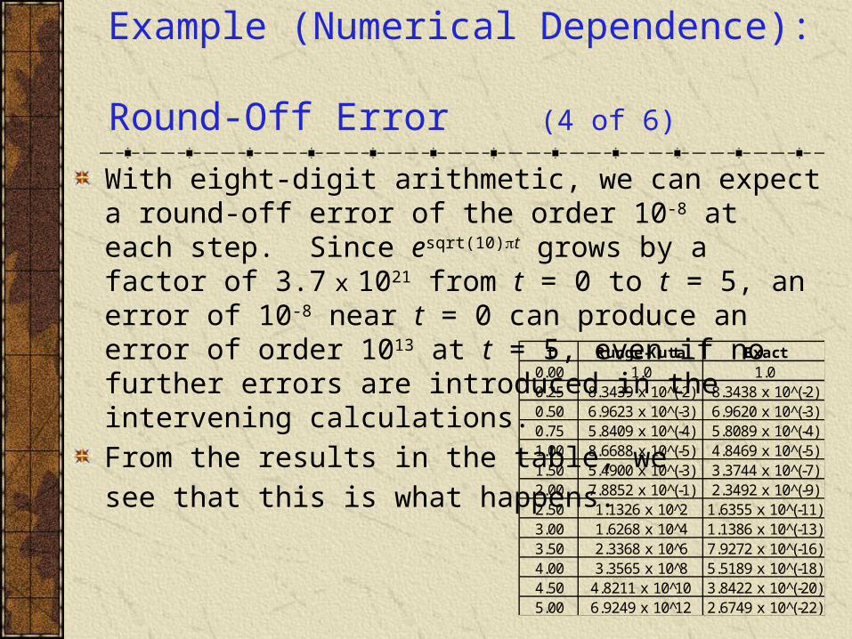
With eight-digit arithmetic, we can expect a round-off error of the order 10-8 at each step. Since esqrt(10)t grows by a factor of 3.7 x 10²¹ from t = 0 to t = 5, an error of 10-8 near t = 0 can produce an error of order 1013 at t = 5, even if no further errors are introduced in the intervening calculations.
From the results in the table, we
see that this is what happens.
t Runge-Kutta Exact0.00 1.0 1.00.25 8.3439 x 10 (̂-2) 8.3438 x 10 (̂-2)0.50 6.9623 x 10 (̂-3) 6.9620 x 10 (̂-3)0.75 5.8409 x 10 (̂-4) 5.8089 x 10 (̂-4)1.00 8.6688 x 10 (̂-5) 4.8469 x 10 (̂-5)1.50 5.4900 x 10 (̂-3) 3.3744 x 10 (̂-7)2.00 7.8852 x 10 (̂-1) 2.3492 x 10 (̂-9)2.50 1.1326 x 10^2 1.6355 x 10 (̂-11)3.00 1.6268 x 10^4 1.1386 x 10 (̂-13)3.50 2.3368 x 10^6 7.9272 x 10 (̂-16)4.00 3.3565 x 10^8 5.5189 x 10 (̂-18)4.50 4.8211 x 10^10 3.8422 x 10 (̂-20)5.00 6.9249 x 10^12 2.6749 x 10 (̂-22)
Example (Numerical Dependence): Unstable Problem (6 of 6)
Our second order equation
is highly unstable.
The behavior shown in this example is typical of unstable problems.
One can track the solution accurately for a while, and the interval can be extended by using smaller step sizes or more accurate methods.
However, the instability of the problem itself eventually takes over and leads to large errors.
0,010 2 tyy
Summary: Step Size
The methods we have examined in this chapter have primarily used a uniform step size. Most commercial software allows for varying the step size as the calculation proceeds. Too large a step size leads to inaccurate results, while too small a step size will require more time and can lead to unacceptable levels of round-off error. Normally an error tolerance is prescribed in advance, and the step size at each step must be consistent with this requirement.The step size must also be chosen so that the method is stable. Otherwise small errors will grow and the results worthless. Implicit methods require than an equation be solved at each step, and the method used to solve the equation may impose additional restrictions on step size.
Summary: Choosing a Method
In choosing a method, one must balance accuracy and stability against the amount of time required to execute each step.
An implicit method, such as the Adams-Moulton method, requires more calculations for each step, but if its accuracy and stability permit a larger step size, then this may more than compensate for the additional computations.
The backward differentiation methods of moderate order (four, for example) are highly stable and are therefore suitable for stiff problems, for which stability is the controlling factor.
Summary: Higher Order Methods
Some current software allow the order of the method to be varied, as well as step size, as the method proceeds. The error is estimated at each step, and the order and step size are chosen to satisfy the prescribed tolerance level.
In practice, Adams methods up to order twelve, and backward differentiation methods up to order five, are in use.
Higher order backward differentiation methods are unsuitable because of lack of stability.
The smoothness of f, as measured by the number of continuous derivatives that it possesses, is a factor in choosing the order of the method to be used. Higher order methods lose some of their accuracy if f is not smooth to a corresponding order.


![[William E. Boyce, Richard C. DiPrima] Elementary (BookZZ.org)](https://static.fdocuments.in/doc/165x107/55cf9326550346f57b9c2ea7/william-e-boyce-richard-c-diprima-elementary-bookzzorg.jpg)