ELSEVIER Journal of Econometrics 75 11996) 239 261

i m

JOURNAL OF Econometrics

Bounding posterior means by model criticism

S h i g e r u I w a t a

Department of Economics, Unit~ersiO; of Kansas. Lawrence, KS 66045. USA

(Received March 1994; final version received March 1995)

Abstract

To handle the sensitivity of posterior inferences to prior choices, Leamer 11983) suggests that one specify a class of priors that is large enough to include all possible priors and then derive the set of posterior distributions associated with it. In many practical situations, however, this set of posteriors turns out to be too large to be useful even with informative data. Frequently, the culprit is those dogmatic priors that are not compatible with the data information and removal of such priors often significantly narrows down the set of posteriors. When a complete elicitation process requires excessive time and resources, a feasible alternative is to use the sample information to help the researcher identify unreasonable priors. The approach proposed in this paper is to bound the posterior means of the regression parameters by 'Model Criticism' in the sense of Box (1980). More specifically, it restricts priors to those for which the predictive density of the observation is not too small. A set of posteriors is then ol;tained for this restricted class of priors. The proposed procedure will be applied to U.S. money stock data Io examine the behavior of the proposed bounds.

Kqv words: Bayes factor; Predictive density;/:-statistic J EL class![icat ion: C 11; C 12; C20; C 52

| . lnCroduction

When the model and tile prior, two most important ingredients of Bayesian statistics, are both specified correctly, the Bayesian procedure provides a system- atic and coherent method of statistical estimation and inference. In reality,

! would like to thank Donald Lien, Joe Sicilian, Anne Sibert, I)e-Min Wu, two anonymous referees, an associate editor, and Arnold Zellner for their helpful comments and suggestions. This research was supported by University of Kansas General Research allocation # 3093-X-0-0038.

0304-4076/96/$15.00 ,~'~ 1996 Elsevier Science S.A. All rigi~ts reserved SSDi 0304-4076(95101759-7

240 S. lwata /Jot,rnal t?]'Economeo'ics 75 (1996) 239-261

however, misspecification of models and of priors is the rule rather than the exception. Such consideration explains a recent emphasis on model checking in classical statistical disciplines and prior sensitivity analysis in Bayesian ~tatistical practice (for the latter see, e.g., Dickey, 1972; Leamer, 1978; Berger, i984).

Let us consider the following situation. Suppose first that, due to previous experience and other information, a researcher has adequate confidence in his basic specification of the model; thus, for the moment, his concern centers on his prior specification. It is furthet a~sumed that the researcher, on the one hand, has ~ pretty g,.,od ~',ess, based on ~ome economic theory, about the magnitude of particular linea~- combinations of the coefficients of his regression. On the other hand, he has some difficulty quantifying the accuracy of his guess. An important special case included in the above description is the well-known situation in which a researcher who has a long list of potential regressors wonders which of them should be included in the regression and which should be omitted. There is a large literature on this subject, and many classical procedures have been suggested. From a Bayesian standpoint, the coefficient parameters for those regressors which the researcher is uncertain whether to exclude should have a prior mean (or other central tendency) equal to zero and a prior variance which ~ierJends on how certain he is about his guess.

In the above conte~t, L,:amer (1982 ~ showed that, when a prior and a sample both have normal distributions, there exist~ a bounded set in which any posterior means of the regression coefficients must lie regardless of the prior variance, t in many empirical situations, however, the above bounds are found to be too wide even when the conventional tests indicate fairly unambiguous sample evidence (see, e.g., McAieer et al., 19851. In fact, the bounded set would not be aft'coted by any change in the variance of regression errors, in particular, the parameter point which satisfies the prior restrictions exactly (i.e., the dog- marie point) would always be included in the bounds, whatever slrong evidence the sample may provide against such restrictions. This is because the initial prior class contains some priors that are so dogmatic that researchers do not learn anything from the sample, even when the sample evidence sharply contradicts such priors. If this is the case, it is very impoltant to develop a sensible way to eliminate the dogmatic priors from posterior inference, thereby obtaining a more reasonable class of posteriors.

There are two ways to eliminate undesirable dogmatic priors from inference. One is to go through a complete elicitation process. However, the question as to which prior, dogmatic or not, belongs to the true class of priors can only be

L Learner (19t, t31 and I.eamcr and I.eonard (1983) developed a procedure for bounding 1t1¢ poslerior means by bounding tile prior ct~varianccs. This needs, however, additional inforrnathm about I.hc priors, and we do not discuss this subject.

S, lwata /Journal of Econometrics 75 (1996) 239-261 241

answered by the ideally designed elicitation scheme, which often requires exces- sive time and resources. An alternative is to use the sample information to help the r~searcher identify unreasonable priors. Though not standard from the traditional Bayesian standpoint, this is sometimes the only feasible course of action, given time and resource constraints. Cooley and LeRoy (i981) and Granger and Uhlig (1990) are two examples.

How then do we judge whether a particular prior is dogmatic'?. The criterion employed here is 'model criticism'. The idea comes from Box (1980), who described the progress of statistical inference as an iteration of two complemen- tary principles: 'criticism' and 'estimation'. A complete statement of the model is provided by the joint density f(y,0)=f(ylO)n(O), where f (yl0) is the data density of y and re(0) is the prior on 0. Alternatively, this join! density can be factored as f (y ,0 )=f (Oly) f " (y ) , where f " ( y ) = ~of(ylO)rc(O)dO. Given the truth of the model, the posterior distribution f(0ly) provides all relevant estimation inferences about 0. However, this factor is totally uninformative about how likely the data is to be generated by the model. Such plausibility of the model is given instead by the predictive density, f~(y). The traditional Bayesian tends to concentrate on f(01y) and does not pay much attention to f"(y). When the elicitation scheme is not ideal, however, the sample information is useful in identifying unreasonable but influential priors. Too small a predic- tive density casts a doubt on the adequacy of the priors. An approach proposed in this paper is to bound the posterior means of the coefficients by 'model criticism' in the sense mentioned above. 2 More specifically, it restricts priors to those for which the predictive density is not less than some small positive scalar ::. A set of posteriors is then obtained for this restricted class of priors. Interestingly, it turns out that the criterion implied by the proposed approach has a direct relation to those of the previous studies.

The organization of the rest of the paper is as follows. The next section introduces the model and notation necessary for subsequent discussions and reviews previous work on this subject. Section 3 introduces a new criterion for bounds called the 'criticism i~idex' and discusses its relation to other criteria. Section 4 is devoted to derive the bounds on posterior means associated with each of these criteria. In Section 5, the results are applied to an empirical study of U.S. money demand. A brief conclusion is given in the final section.

2 As dclined above, 1he term 'model' here is used in Box's sense, that is, as the product of ./'(yl0), which is usually called the model, and the prior zr(0). Accordingly, 'm{~del criticism' includes not only ~11c criticism against models in the usual scnse but the criticism against priors as we~l. In this paper, wc discuss mainly thc proccdure For checking whether priors arc reasonable. To aw)id possible confusion in terminology, in fl~c rest of the paper wc use the term "modcl" in the slandard sen:~c,

referring Io .[(ylO}.

242 S. lwata /Journal of Econometrics 75 (1996) 239-261

2. Bounding posterior means

2.1. The model and notation

We consider a regression model,

y = x/3 + u, (l)

where y is a T × 1 vector of observations on the dependent variables, X is a T × k matrix of explanatory variables, /3 is a vector of unknown parameters with dimension k, and u is a T × 1 vector of unobservable errors. The elements of u are assumed to be independently drawn from a normal population with zero mean and finite variance a 2 with unknown value. A researcher is assumed to have some prior information about linear combinations of the coefficients R/3, where R is a p × k matrix. The following arrangement allows us to partition the parameter vector/3 into two subvectors: one with informative priors and the other without them. Let Q be some ( k - p)× k matrix such that [R ' ,Q ' ] is nonsingular and RQ' = 0 (note that Q is not unique). Then we can write a prior distribution on 0 = (/3, a 2) as n(0)d0 = n(Q/31R/3, a)n(R/3la)n(a), dQ/3. dR/3" da. Now a prior on 0 is assumed to belong to the class F, which is described as follows. First, a prior on R/3 given a has a normal distribution with mean r and variance aZV for some symmetric nonnegative definite (s.n.n.d.) matrix V. Next, a prior on Q/3 and a 2 are taken to be diffuse such that n(Q/31R/3,a) oc constant and n(a) oc a 1

Let b = (X'X)~ iX'y, the OLS estimator of/3 in (1), and ESS = ( y - Xb)' × (y - Xb). Then the marginal density f ( y l V ) foe" a particular choice of V is

found to be

f (y lV) oc (ICIIWI/IW + VI)'/2(ESS + q),./2 (2)

where C = Q[(X'X) t _ (X'X)tR'W tR{X'X) ~ t]Q', w = R(X'X)~R', q = q(V) = (Rb - r)'(W + V) ~ t(Rb - r), and v = T - k + p.

In the rest of this section we introduce the basic set of posterior means of regression parameters discussed by Leamer (1982) and two restricted sets implied in the literature.

2.2, Feasible ellipsoid

We denote the posterior mean of fl associated with a prior in the class F by /I(V) or simply/~. Then/~ can be expressed as

P, = / ~ { v l = b - ( × ' x ) ' r ' ( w + ,~: ) -~(Rb - r). (3)

When V is nonsingular, this can be written as a more familiar matrix average form: ~ = (X'X + R'V- ~R)- '(X'Xb + R ' V ~r). Let the restricted least square {RLS) estimator of {1) with constraints R / 3 = r be denoted by bR, i.e.,

S. ht,ata / Journal of Economeo'ics 75 (1996) 239-261 243

bR = b - (X'X)- ~R'W- l ( R b - r). It is easy to observe from (3~ that fl reduces to the OLS estimate b as V --, c~, whereas it becomes the RLS estimator bR as V ---,. 0.

The next lemma, which is due to Leamer (1982), shows that fl is bounded in an ellipsoid.

Lemma 1 (Learner). fl is a posterior mean of fl associated with a prior in the class F, if and only !f fl ~ E, where E is a set of fl satisfying

Eft - (b - bR)/2]'A[fl - (b + bR)/2] ~< q/4~ (4)

where A = R 'W- 1R, q = ~/(0) = (Rb - r ) 'W- l(Rb - r), and W = R(X'X)- IR' as defined previously. []

The ellipsoid (4) is referred to as the 'feasible ellipsoid' by Leamer. Note that two estimator points b and bR are symmetrically located on the surface of the feasible ellipsoid with respect to its center (see Fig. 1). Now let S be the set of all p x p s.n.n.d, matrices and let S~ denote the set of V's satisfying (3) for a particular fl, or the collection of all prior covariance matrices that would lead to the posterior mean equal to ft. Then S may be decomposed into equivalent classes S~'s. In other words, S~nS~. = 0 for fl -¢: fl' and S = I,.3~trS~. Clearly, for any

~ E except b and bn, the corresponding set S~ is uncountable. The set S,~ plays an important role in the following discussion.

2.3. Compatibility statistic" and F-statistic

In estimating the money demand function, Cooley and LeRoy (1981) pro- posed restricting fl to the set of points for which the classical F-test does not rcject the hypothesis fl = ft. The test statistic is given by

F --- ~/(ps2), (5)

where ~ = ¢(V) = (fl - b)'X'X(fl - b) and s: = ESS/(T - k). Too large a value of ~ indicates, from the classical standpoint, that fl does not appear to be the true value of ft. The restricted set of posterior means for this criterion, therefore, is given by

E,..= {f l~E: ¢ ~<~}, (6)

where ~ is a prescribed positive scalar, usually ps 2 multiplied by the upper ~% quantile of the F-distribution with degrees of freedom p and T - k.

Motivated by a similar idea, Granger and Uhlig (1990) suggested the bounds implied by the condition associated with R':, the coefficient of determination. Let R~,R 2, and R 2 denote the R 2 of the regression when/3 is estimated by fl, b, and bn, respectively. Granger and Uhlig required that R~be not too small, or more specifically,

>t - (1 - ,o)n?, + , o n e , (7)

244 S. Iwata / Journal of Econometrics 75 (1996) 239-261

with to ~ [0, 1] selected by the researcher. 3 This condition is actually identical to the criterion ~. based on the F-statistic. To see this, let 6 = y - Xfl = e +

2 X(b - fl), where e = y - Xb. Then we have 6'~ = e'e + ¢, so that the Rti may be written as

2 ~'~ ESS + ~ R a = 1 5,"5' - 1 5"5' = R 2 - ---:--~,~, (8)

or ~ = (R;; - R~)~'~, where ~ = y - ly with .9 = l ' y / T . Since R ~ = R 2 - q /~ 'y ,

we may express R2(to) as

/~2(uj) = R 2 - eoq/~'~. (9)

Using (8) and (9), the condition (7) is equivalent to ~ <~ toq. Hence, the bounds suggested by Granger and Uhlig (1990) are given by (6) with ~ = toq.

Theil (1963) and Box (19S0) independently proposed a more explicit use of the sample information to criticize priors. Their assessment is based on q = ( R b - r)'(W + V)- ~(Rb - r), as defined in (2). A large value of r/indicates that the prior restriction on fl does not appear to be consistent with the sample information. The statistic q, therefore, can be used for a chi-square test for checking 'compatibility of prior and sample information' (Theil) about location. We refer to r/as 'compatibility statistics'. Theil and Box suggested that priors which fails the compatibility test should be suspected. Although neither author directly addressed the class of posteriors, their test implies that the reasonable bounds of fi are described by

l::c ~ {fi c !~':, ~< ,~I, (10)

where i / is a prescribed positive scalar, usually tile upper g% quantile of tile chi-squared distribution with k---p degrees of freedom. Note also that ¢(0) = q(0} = q, that is, if the prior becomes dogmatic, the ¢ and q statistics reduce to the usual F-statistic.

3. A n e w a p p r o a c h

3. !, B¢o'es f l w t o r

We now derive a bounded set of estimates induced by 'model criticism'. Consider first the Bayes factor B(Vt, V2) =.f(ylVi ) I f ( y I V2), which compares

~ Those specilicatmns satisfying condition (7) for a small r,J 'may be considered as being 'reasonable' st')ecifications as riley are not far from file 'best' model in lerms of goodness-of-til, as measured by R 2' ((h'anger and Uhlig 1990, p. 160).

S. hvata /Journal of Econometrics 75 (1996) 239-261 245

the plausibility of the prior represented by V~ with that by V2.* Note that using (2), this Bayes factor can be written as B(V~, V2)= m(V~ )/re(V2), where

re(V) = IW + Vl- ~"2 [ESS + q ( v ) ] -':2. (11)

Now taking the infimum of B ( V t , V 2 ) with respect to V2, we define B(V) = m(V)/supv re(V), where the supremum is taken over all p ×p s.n.n.d, ma-

trices. In what follows we shall derive the bounds on posterior means of fl by restricting the value of B(V) to be not too small. 5 Uncountabflity of S~ (the set of V's corresponding to the posterior mean fl) mentioned previously, however, implies that B(V) is not uniquely determined for a given posterior mean B. Our approach is therefore based on

B*(~) = s u p B ( V ) = sup m(V) /sup re(V). V~S~ V~Si'~ V

(12)

If fi satisfies B*(f i )< ~: for a small positive ~:, it follows by definition that B(V) < ~: for any V ~ $1~, 6 implying that such fl is an unlikely estimate, whatever prior covariance is selected from S~. Thus B*(fi) can serve as a conservative criterion for model criticism. The bound on the posterior mean of [I obtained by the condition B*(fl) >/~: gives a set of fi's associated with at least one prior in F that does not contradict the sample information so sharply.

3.2. Criticism index

To calculate B*lfl), we need the following lwo lemrnas, which provide the value of V corresponding to each suprernurn of the last expression of (I 2).

Lemma 2. For any fl~ E, re(V) is maximized sul~ject to V ~ S~ by chtmsinq the prior c I' such that R//la 2 ,--. I (r, a2Vti), where Vti = (R/~ - r)dlRfl - r/' with d t = (R/~ - r ) 'W ° l R ( b - / / ) .

Pro¢!/: lwata (1992) has shown that re(V) is maximized when V is of rank one. Note also that d > 0 when //~ E. V~ ~ S/i may be verified by direct calcu- lation. []

* Many authors use f, he posterior odds or the Bayes factors to evaluate both alternative rnodels and their associated priors in their empirical work. See, e.g., a special issue of this journal on Bayesian empirical studies in economics and linance, edited by Poirier {1991 i.

s There are a couple of technical reasons for using BIV) instead of a more direct f(Yl V I as a criterion of criticism. First, unlike ,flylV 1, B{ V I is invariant to the choice tff Q {i.e., the ICl's are canceled out). Second, since B(V) can be expressed as a function of m(V), singtdarity of V d~es not cause

a problem.

~'This claim follows by noticing that for any V ~ Sil, B(V) ~< supv. s~ B(V) = B*(fl) < i:.

246 S. hvata / Journal o f Econometrics 75 (1996) 239-261

Lemma 3. m(V) is maximized by choosing the prior ~ F such that Rflltr 2 ~-A," (r, aEv*), where V* = (Rb - *)d*(Rb - r)' with d* = max{0,(v - 1)/ESS - q- t} and q = (Rb - r) 'W- t(Rb - r) as defined in Lemma 1.

Proof. This is a corollary of lwata (1992). []

For interpretations of the above results, see Iwata (1992). We now show that B ' l # ) can be expressed in terms of two key statistics introduced earlier: r / = ( R b - r)'(W + V) - t (Rb - r) and ~ = (fl - b)'X'X(# - b). For this pur- pose, note first that (3) implies b - fl = (X'X)- tR'(W + V ) - ' ( R b - r) where V e Sty. Pre-multiplying both sides of this identity by W - t R and recalling W = R I X ' X ) - tR', we find W - tR(b - #) = (W + V)- t(Rb - r). From this we obtain an alternative expression of r/ as ~/= ( R b - r ) ' W - t R ( b - fl). An important implication of this result is that t/ as well as 4 are invariant with respect to the choice of V eSti. Next, it follows from the relation ( X ' X - R ' W - t R ) ( X ' X ) - t R ' = O and the expression b - f l above that ( # - b ) ' (X 'X- R ' ~ ' - t R ) ( # - b ) = 0, which implies that ,~ may be expressed alternatively as 4 = ( f l - b ) ' R ' W - 1 R ( f l - b ) = (b - f l ) ' R ' ( W + V ) - t ( R b - r). Further, using these expressions, we find (Rfl - r) 'W- l(Rb - r) = q - r/ and d - t = ( R f l - r ) ' W - t R ( b - f l ) = r / - 4. Finally, combining these two, we obtain

- r ) ' W - r ) = , i - 2,1 + 4 .

We are now ready to calculate B*(fl). First note that the invariance property of r/(V) implies that r/(Vti) = ~?. Next, plugging the expression of Vii in Lemma 2 into (11), and using the identity I W + V # l = l W l [ l + d ( q - 2 r / + 4 ) ] = Iwl(q ~ q)/01 ~- ¢), we obtain supv,~s,~ re(V) = IWl '/2[(¢1 - ' I ) M - ~ ) ] - I / 2 X (ESS + t/) ~'/2. Now replace Vti and d respectively by V* and d* and notice tl(V*) = ESS/(v - 1) and IW + V*l = IWl(l + d'q) = I W l [ l v - I)q/ESS] assuming d* > 0. We then obtain supvm(V) = IWl-t/2q-a/2 v-~2 × [ESS/(v - 1)]-'-t~/.'.. Substituting above two expressions into (12), we obtain

\ v - l ] L q - ~ l J

From the above, the set of the posterior means of # implied by condition B*(fl) t> ~: can be written as

q - ~l~ t/2 Ev=-{ f l :4~<~} with t k = \ ~ l _ ¢ / IESS+~I) "~2, (13)

where ~ =t :M and M = ql/2v":2[ESS/(v- 1)] "- ')/2. We refer to q5 as the criticism i.,dex.

S. Iwata / Journal o f Econometrics 75 (1996) 239-261 247

Each of the three statistics tp, r/, and ~, introduced so far, provides a criterion for choosing reasonable estimates from E. What then are the relations between these statistics? First, as the sample size gets large, the criticism criterion (13) is well approximated by the compatibility criterion r/because, as T ~ ~ , ~b tends to an increasing function of ~I only. Second, the criticism criterion integrates the two other criteria in the sense that ~b depends on fl only through r/and ~. There is, however, a most important difference between the ¢ criterion and the other two. The ¢ criterion treats fljust like any point in ~k, ignoring the important fact that fl is a logical compromise between the sample information and the prior information. The ~ criterion criticizes the final output fl according to how far

lies from the point most favored by the sample without any direct reference to the priors. This is what makes most Bayesians uncomfortable. However, the other two criteria directly criticize the priors. The t/ criterion examines the reasonableness of a given prior in light of the sample. The ~ criterion concerns the plausibility that the observed sample comes from the model and the prior combined.

4. Deriving the bounds

In many practical situations, the researcher's interest often centers on a par- ticular linear combination of the components of ft. In what follows, we derive the bounds on ~'fl implied by the condition that fl belongs to either E, Ee, Ec, or Ep, given in (4), (6), (10), and (13), respectively, where ~b is a k-dimensionai vector of constants.

To determine the bounds implied by different criteria, it is useful to split the optimization procedure into two steps. In the first step, we fix r/and ~, and derive the bounds on q~'fi conditional on the value of(p/, ¢). Then, in the second step, the bounds specilic to different criteria will be obtained under the restrictions on r /and ~ imposed by those criteria.

Lemma 4. The extreme values of a linear combination and ~ are

= ( 1 - +

___ A ,t2 {q~'(X'X)- '~, - [¢'(b - ba)] 2 }'/2/q,

where A = q~ - ~l 2. []

of fl conditional on t 1

(14)

Note that the center of bounds (14) is a scalar-weighted average of ~b'b and ¢'bg with the weight equal to 01/q) e [0, 1]. This bounds degenerate to the above point when i/J happens to be proportional to the vector R'W ~(Rb - r), since then q~b'(X'X)- l~b = [~b'(b - ba)] 2. The quantity A measures how far fl is away

248 S. lwata /Journal o f Econometrics 75 (1996)239 261

from a scalar-weighted average of b and br. 7 Lemma 4 can be used to obtain specific bounds by further op t imiz ing (N; ;:r.~ier partict~lar restrictions on (r#, ~.). We begin with the case in which/7 belongs ~ ,: the set E given in (6). The resulting bounds are expected to be the widest and are not restricted by any criticism. To derive the bounds on Ip'fl, note that inequality (4) holds iff q - <7 >/0. Maxi- mizing or minimizing (14) with respect to r / a n d ~. under the condi t ion i,/1> ~, we obtain the following result.

Proposition I. When fl belongs to the set E given in (6), a linear combination of posterior means ~s'fi lies in the interval Io = (lo, Uo), s where

1 Io = 7{ t / s ' (b + b r ) - [ q l / s ' ( X ' X ) - ' l / s ] '"2} ,

_t .¢,l/~h Uo 2 t 'e ,~ + b r ) + [ q ~ b ' ( x ' x ) - 1'1'11121>

provided that ip ' (X'X)-IR' d: 0 . / f l~ ' (X 'X) - JR ' = O, then the interval de,qenerates to the point ~s'~ = $'b. []

Note that when the vector ~s lies in the null space of RN t, the posterior mean of ~b'[I is equal to the unrestricted OLS est imate regardless of the priors. This proper ty will be inherited by all three bounds on [L because Ec, Ev, and E~, are all subsets of E. Hence, we assume in the following analysis that I / / ( X ' X ) ~ t R' ¢ {}. Now define

I ( h ) = h i l , v l / ( X ' X } I k'(b ......

' I • q ' = 7 [ q + q [ t / d ( b o- b r ) ] ~ ' / q / ( X ' X ) I I [ j } i : z ] .

!

.g . . . . [ q - { q U ¢ / ( b -

Then we obtain the following proposition, the part (it) of which is stated u~ider the assumpt ion ~ ' ( b - b r ) ~ 0; if it is negative, set ~ = -~b and the restllt applies.

This can be seen by noticing that A = 0 when V is proportional to W, in which case/l reduces to the posterior mean associated with Zellner's (1986) g-prior. It is well-known tllat the latter is a scalar-weighted average of b and br.

I.camer ( 1982, p. 7311 showed how to derive 1.. hut hi~ kcmmas 2 and 3 do not apply to the case m which the restriction matrix R is not square and hcncc the matrix A (in our Lcmma 1 and his I,emma 31 is singular (see the Remark on kemma A.I. in the AppendixL

S. Iwata / Journal of Economettqcs 75 (1996) 239-261 249

Proposition 2. (i) Suppose fl belongs to the set Ec given in (10). Then a linear combination t f posterior means q.,'fl lies in the interval Ic = (i~, u~), where

~ = .f) { ¢,'(n, + b.,) - U,j~,'(×'x)-'~,3',~ } [ ( 1 - - q/q)qJ b + ( q / q ) q / b e - - l(q)

= .f'{,/,'(b + h , . ) + [,~,,O'(X'X)-'~]'/~} u,. [ ( I - q/q)~, b + (q/q)q/b~ + l(q)

!f O >.>..q., otherwise,

i f#>~g_, otherwise.

(ii) Suppose fl belongs to the set Er given in (6) and ~b'(b - bR) >i 0. Then a linear combination of posterior means ~b'fl lies in the interval Iv = (ly, us), where

is = (1 , - ~/q),p b + (~./q)q, b . -

b - I-~-q/(×'X)- ',/,-I '/~

'4,] '~} ff ~->~ g+,

I(~) /f g+ > (>~ a2/q/(X'X)- '~b,

otherwise,

f 1 f , , , t ~tqJ ia 4- bR) 4- [q~ ' (X 'X)- '~b] ' / ' } !f ~>~ ,q_,

uy = (1 -- f/q)~b'b + (~-/q)~b'bR + l(~-) otherwise. []

The bounds lc have been derived by Granger and Uhl ig (1990) in terms of t r igonomet r i c formula . Wha t is interest ing here is that the behavior of the b o u n d s Ic and Iv turns out to be qui te similar. In fact, if only the set of RLS est imates rather than the set of all Bayes estimates is our concern, 9 the two criteria would coincide. The bounds on ~,'fi implied by the criticism index are given by the next proposi t ion .

Propositiml 3. When fl belongs t,~ the set E~, given i~a (13), a linear ('omhination of posterior means ~/J'fi lies in the interval II, = (ll,,uv), with

I I, =-= (I - -q , / q )~ j /b + (q,/q)q/bu

- A~/~-{q~P'(×'X)~qJ - DP'(b - bR)]2}~"2/q,

u~, = (1 - q*lq)q/b + (q*/q)q/bR

- A*I/2{q~O'tX'X)-'¢ - [¢ ' (b - bR)]2}l/2/q,

where q, is the value t f q minimizing the lower bound in (14), q* is the value of q maximizing the upper bound in (14), both subject to q(ESS + q)"/tp 2 < ~l < q; A. = A(q,) and A* = A(q*) with A(q) = (q - q)[q - q(ESS + q)"/q52]. []

'~ The set of all Bayes eslimates arc given by (4), whereas the set of all RLS estimates is rcpresemed by (4) with its weak inequality replaced by equalily, or geomclrically the skin of the ellipsoid rather than its entire body.

250 S lwam /Journal of Ecopometrics 75 (1996) 239-261

Feasible Ellipsoid (100-~t)% Confidence Ellipsoid

Ep

E

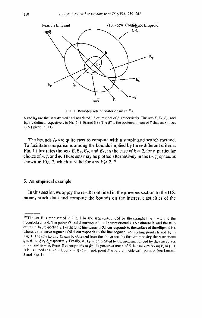
Fig. !. Bounded sets of posterior mean fl's.

b and bR are the unrestricted and restricted LS estimators of fl, respectively. The sets E, El.., Ec, and Ee are defined respectively in (4), (6), (10), and (! 3). The/l* is the posterior mean of/~ that maximizes re(V) given in (11).

The bounds Ij, are quite easy to compute with a simple grid search method. To facilitate comparisons among the bounds implied by three different criteria, Fig. 1 illustrates the sets E, Ee, Ec, and El,, in the case of k = 2, for a particular choice ofQ, ~-, and t~. These sets may be plotted alternatively in the 01, ~.) space, as shown in Fig. 2. which is valid for any k >/2. t °

5. An empirical example

In this section we apply the results obtained in the previous s,~ction to the U.S. money stock data and compute the bounds on the interest elasticities of the

I'~The set E is represented in Fig. 2 by the area surrounded by the straight line ~1 = ~ and the hyperbola A = 0. The points O and A correspond to the unrestricted OLS estimate, b, and the RLS estimate, bk, respecti~,ely. Further, the line segment OA corresponds to the surface of the ellipsoid (41, whereas the curve segment OBA corresponds to the line segment connecting points b and bR in Fig. 1. The sets Ec and E~. can be obtained from the above area by further imposing tile restrictions ~O ~< Pi and c~ ~< ~, respectively. Finally, set El, is represented by the area surrounded by the two curves A = 0 and ~ = ~. Point B corresponds to/~*, the posterior mean of [J that maximizes re(V} in (I 1). It is assumed that tl* = ESS/(~ .... I} < q; if not, point B would coincide with point A (see Lemma 3 and Fig. I).

S. iwata / Journal qf Econometries 75 (1996) 239-.261

t~=O

q l I / ' ~ A

rl=~

251

! i

o n* n q rl

Fig. 2. Bounded sets in the 0/,¢) space.

The ~* and q* are respectively the values of ~ and q associated with the prior that maximizes re(V). The quantity q is defined in Lemma 1.

demand tbr money. The data set analyzed here was originally studied by Cooley and LeRoy (1981). 11 The basic regression model is presented as model 1 of Table 1, in which real money demand is explained by two interest rates (90 days T-bill nile and S&L passbook rate) and other variables including real income and inflation rate. A trouble with many empirical studies using the above type of regression models is that the estimated interest elasticities are very sensitive to which variables are included in the right-hand side. Cooley and LeRoy (1981) computed the bounds lo (the extreme bounds) on the sum of the coefficients of the interest rate variables and found that the computed bounds tend to have conflicting signs. From this observation, they concluded that significant nega- tive interest elasticities reported in a number of empirical studies are due more to 'the unacknowledged prior beliefs of the researcher" than to 'the information

11 The author would like to thank Professor Cooley who kindly made their data available to him. The data are quarterly and the observation period is from 1952.11 to 1978.1V.

252

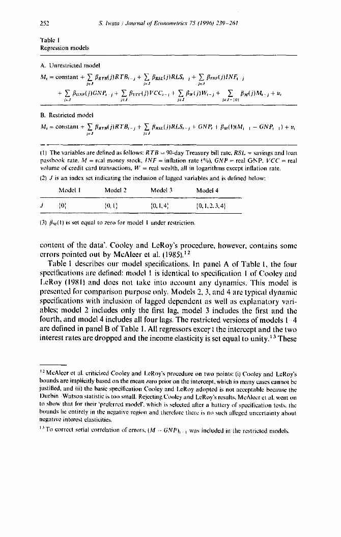
Table I Regression models

S. Iwata /Journal of Econometrics 75 (1996) 239-261

A. Unrestricted model

M, = constant + ~ [IrT~(jIRTB,_j + ~ [3rsL(j)RLS, j + ~ [~,N~.(jllNF, . j j~J jeJ jeJ

+ ~ fi,~.,.p(j)GNP, j + ~. flvcc(j)VCC, j + ~ flw{j)W,-j + ~ flm(j)M,-j + u, j eJ j eJ j~J j~J- ',O}

B. Restricted model

M, = constant + ~ [Irra(j)RTB,-j + ~ flrsL(j)RLS, j + GNP, + [~(I)(1Vl, i - GNPf 1) + u, j~J jeJ

l l) The variables are defined as follows: RTB = 90-day Treasury bill rate, RSL = savings and loan passbook rate. M = real money stock, INF = inflation rate I%), GNP = real G N P , VCC = real volume of credit card transactions, W = real wealth, all in logarithms except inflation rate.

(2) J is an index set indicating the inclusion of lagged variables and is defined below:

Model I Model 2 Model 3 Model 4

.1 f I ,0, [0,1} {0, 1,4', ' "~ ' ~0, I , , , 3,4j

(3) /t~t(I) is set equal to zero for model I under restriction.

content of the data'. Cooley and LeRoy's procedure, however, contains some errors pointed out by McAleer et al. 11985).~2

Table 1 describes our model specifications. In panel A of Table I, the four specifications are delined: model 1 is identical to specification 1 of Cooley and LeRoy 11981) and does not take into account any dynamics. This model is presented for con lparison purpose only. Models 2, 3, and 4 are typical dynamic specifications with inclusion of lagged dependent as well as explanat-~ry vari- ables; model 2 includes only the first lag, model 3 includes the first and the fourth, and model 4 includes all four lags. The restricted versions of models 1-4 are defined in panel B of Table 1. All regressors excel-t the intercept and the two interest rates are dropped and the income elasticity is set equal to unity. 13 These

i 2 McAlecr et al. criticized Cooley and LeRoy's procedure on two points: (i) Cooley and LeRoy's bounds are implicitly based on the mean zero prior on the intercept, which in many cases cannot be justified, and (it) the basic specification Cooley and LeRoy adopted is not acceptable because the Durbin Watson statistic is too small. Rejecting Cooley and LeRoy's results, McAlecr ct al. wen| on to show that f l~r their 'preferred model', which is selected after a battery of specilication tests, the hotmds lie entirely in the negative region and lherefi~rc there is no such alleged uncertainty abou! negative interest elasticities.

13To correct serial correlation of erro,s. (M -- GNP}, t was included in tile restricted models.

S. iwata / Journal q/'Econometrics 75 (1996) 239-261 253

restricted and unrestricted versions of each model are two polar cases included in our class of priors F. More specifically, the priors on the coefficients of two interest rates and their lags [flRrn(.J) and ~Rs:~(.J) for all j ] as well as the intercept are taken to be diffuse, while the prior over all other coefficients is assumed to be distributed as a joint normal with mean zero. ~4

Table 2 reports the estimates of interest rates coefficients together with other statistics. A very small D-W statistic clearly indicates a problem of serial correlation of the errors in model 1, as pointed out by McAleer et al. (1985). Models 2, 3, and 4, on the other hand, do not have such serial correlation problem, show very good fit, and are similarly supported by the data in terms of two Information Criteria (AIC and BIC). ~5 The parameter restrictions are, however, rejected strongly in all cases by F-tests. The S&L passbook rate (RSL) tends to be significant for the unrestricted models, while the T-bill rate (RTB) tends to be significant for the restricted models.

"Fable 3 presents the upper and lower bounds of lr on the sum of the interest elasticities for the above four models.~6 The size of ~o indicates a measure of 'reasonableness' of a given specification suggested by Granger and Uhlig (1990), which was defined in (7). The to equal to 0.0 corresponds to the case in which specification is restricted to the best fitted model (i.e., the unrestricted model), while the ~o equal to 1.0 corresponds to the (unrestricted) extreme bounds. The results reported in Table 3 shows that unlike the case of the velocity of money example of Granger and Uhlig (1990), we do not have to lose so much goodness- of-fit to arrive at the coefficients with conflicting signs in our money demand example. In fact, very high and similar R 2 for each specification renders the Granger and Uhlig type of discussion almost pointless. An alternative dis- cussion, however, can be made in terms of F-value rather than R 2. Note that

~< ~ = ~oq if and only if /; ~< toFo, where Fo = q/ps z is the F-value of the parameter restriction based on the unrestricted OLS estimates. The fraction t~ of file F-value that leads exactly to the 5% critical value in each of the models 2 4 is obtained as the ratio of the last two rows in Table 2, namely 0.05, 0.07, and 0.11. Now look at panels B, C, and D of Table 3. We find the conflicting signs at even smaller values of t,J.

Table 4 presents the upper and lower bounds of I~, on the same sum of elasticities for the four models. Here the size of ;:* indicates a measure of

t,~ An exception is fl,m,(0}, which has unit mean. Also I~¢M{ 1} - fl~;.~e{1 } is assumed to have zero prior

mean.

1 .~ M-;dc! 4 could p,.~ssib!y be overparametrized (35 regress~rs with 103 observations). The intent of including this specilication is, however, to show that the bounds become wider still for a larger

model.

~' We obtained a similar pattern of the bounds of It-, which are not reported here.

T a b l e . "~

Regress ion resul ts

M o d e l ! M o d e l . ~

RTB~O}

R TB~II

M o d e l 3

RTB[2i

RTB[31

RTB~4J

RSL{Oi

RSL( 1 b

M o d e l 4

RSL(21

RSL[3)

RSL(4I

Unres t . Rest. Unr~:sL Rest. Unres t . Rest. Unres t . Rest.

0.010

(0.011} 0.057**

(0.021} - 0.091 - 0.020** - 0.003 - 0.016"*

iO.OO31 {0.006) (0.003) (0.006)

- 0.004. 0 .023"* - 0.003 0.018"*

i0.003~ qO.O06) 10.004} (0.006)

0.007* 0.006

(0.003) (0.004)

- 0.939**

10.055~ - 0.1 t3" - 0.146 - 0.104" - 0.161

~0.052J 10.1031 (0.051) (0.103)

0.105" 0.148 0.073 0.177 ~0.050~ [0.10 ! ) (0.058) (0.118)

0.030 - 0.036

(0.029) (0.047)

- 0.175"

c0.069i

- 0.004

(0.004)

- 0 . 0 0 5

(0.006)

0.009

(0.007)

- 0.003

(0.006)

0.004

(0.004)

-- 0.020** (0.007)

0.027*

(0.012)

- 0.011

10.013)

0.018

(0.012)

- 0.007

(0.007~

- 0.088 (0.052)

0.064 (0.080)

- 0.030

(0.081)

0.018

(0.088)

0.024 (0.061)

- 0.108

(0.102)

- 0.123

(0.158)

0.318"

(0. ! 60)

- 0 . 0 0 1

( 0 . 1 6 0 )

- 0.102

(0.101)

Ir ,,,b

, . , , .

7.;"

I h , a

R 2 0.707 - 0.994 0.972 0.995 0.974 0.996 0.976

D W 0.063 0.055 1.55 1.96 1.73 1.95 2.02 2.03 D - h - 1.78 0.07 1.00 0.09 - 0.81 - 0.38

Q{25~ 521 ** 517** 30.7 23.5 35.7 305 15.4 29.8 Q{30t 580** 534** 43.4 28.5 44.9* 37.0 18.6 33.8

A I C - 4.23 - 2.80 - 7.98 - 6.59 - 8.04 - 6.50 - 8.01 - 6.62 B I C - 6.89 - 5.56 - t0.47 - 9.27 - 10.34 - 9.23 - 9.96 - 9.15

L I K E 233.3 152.5 436.9 355.0 435.2 347.6 447.6 352.7

F 88.1"* 42.4** 28.3** i 5.7** 5% c.r. 2.46 2.11 1.88 1.70

{1~ The columns headed by the labels "Unrest ' and "Rest" display the coefficient estimates for the unrestricted and restricted models defined in Table 1,

respectively. The numbers in the parentheses below the estimates are the standard errors. z

{2) The figure in the parentheses after the variable acronym indicates the number of lags applied to the variable in question. For example, GNP{I) stands ~

for G N P, _ i . "~

13t "R-'" for each model is calculated according to the definition in the text [e.g., Eq. {81]. As a result, it becomes negative for the restricted model 1 and not ~ "M

reported in the above table.

(4) 'D W' and "D-h" stand for the D u r b i n - W a t s o n statistic and the Durbin 's h test statistic, respectively; "Q{ j) ' stands for the Box-Ljung Q-test statistic of ~,e j lags: "AIC" and "BIC" stand for the Akaike and Schwartz laformat ion Criteria, respectively; ' L I K E " stands for the maximized value o f the log-likelihood;

'F ' stands for the F-value for testing respective restricticn'.; while "5% c.r." indicates the 5% critical value for the corresponding F-test.

{5) The superscripts * and ** indicate, respectively. 5% and 1% significance for a respective test.

256

Table 3

The bounds iv

S. lwata / Journal of Econometrics 75 (I 996) 239-261

Size o f ,t,J

Bound 0.0 0.01 0.05 0,1 0.3 0.5 1.0

A. Model 1: /JR~-8(0) + / l a s t ( 0 )

Upper - 0.165 - 0.100 0.008 0.046 0,062 0.062 0.062

Lower - 0.165 - 0.255 - 0.452 - 0.571 - 0.869 - 1.071 - 1,223

!

B. Model 2: ~, #~ro(J) + [~asL(J) j=(}

U p p e r - 0.012 0.011 0.038 0.058 0,098 0,111 0.111

Lower - 0.012 - 0.035 - 0.061 - 0.079 - 0.112 - 0,119 - 0.119

C. Model 3: ~, [InrB(j) + llasL(J) )e ',o, I ,al

Upper 0.001 0.039 0.084 0.115 0.173 0.187 0.187

Lower 0.001 - 0 . 0 3 7 - 0 . 0 8 3 - 0 . 1 1 6 - 0 . 1 7 9 - 0 . 1 9 8 - 0 . 1 9 8

4

D. Model 4: ~,, [tRra(j) + [~ast,(J) j=O

Upper - 0.010 0.030 0.078 0.111 0.175 0.192 0.192

Lower - 0.010 - 0.1)50 - 0.097 - 0.131 - 0.194 - 0.211 - 0.211

Each pair of figures in the rows labelled 'Upper' and ' L o w e r ' gives, respectively, the upper and lower bounds of Iv [g iven it) i)roposition 2(ii)] o n the sum of the imcrest ehLsticities it) each mode l . The size o f , J ind ica tes a measu re of ' r easonableness" of :t given prior suggested by G r a n g e r a n d tJ hlig (I 990), def ined it) (7L

plausibility of a given prior in terms of the infimum of Bayes factors (12), or B*(IT) ~> ~: ~ 10 -~'. The ~:* equal to 0.0 corresponds to the case in which only the prior for which B*(fl) equal to unity is allowed. 17 As e* gets large, a wider class of priors or specifications becomes allowable, and the ~:* equal to infinity corresponds to the (unrestricted) extreme bounds. Instead of asking which value of ~:* is most appropriate for identifying unreasonable priors, we first consider how small the ~:* must be in order to have both bounds in the negative region. This latter question is easy to answer. From Table 4 we see that the upper bound for model 3 is already positive at ~:* = 0. For models 2 and 4 the upper bounds change their signs somewhere between ~:* = 0.0 and 1.0, most likely the value less than 0.5. Since ~: = 10 '~', the ~:* equal to 0.5 indicates that the plausibility

t 7 T h e assoc ia ted /~ , ~, and ~1 can be found in Figs. 1 a n d 2, labeled as/~*, 4", a n d q*.

S. lwata / Journal of Econometrics 75 (1996) 239-261 257

Table 4 The bounds I~,

Size of ~:*

Bound 0.0 1.0 2.0 4.0 10 20 40

A. Model I: flRrB(0) + firm.(0)

Upper - 0.167 -- 0.068 - 0.033 0.001 0.060 0.062 0.062 0.062 Lower - 0.167 - 0.287 - 0.344 - 0.431 - 0.651 - 0.974 - 1.223 - 1.223

I

B. Model 2: ~. [inrn(j) + flRsl.(J) j=o

Upper - 0.012 0.014 0.025 0.040 0.074 0.107 0.111 0.11 ! Lower - 0 . 0 1 2 - 0 . 0 3 8 - 0 . 0 4 8 - 0 . 0 6 2 - 0 . 0 9 3 - 0 . 1 1 8 - 0 . 1 1 9 - 0 . 1 1 9

C. Model 3: ~ [tRrB(j) + flRs~.(j) j~ ',O. 1.4',

Upper 0.001 0.041 0.058 0.080 0.133 0.182 0.187 0.187 Lower 0.001 - 0.040 - 0.057 - 0.082 - 0.135 - 0.190 - 0.198 - 0.198

,4

D. Model 4: ~ flnrn(.jl + flnm.(.Jl j = ( I

Upper - 0.010 0.030 0.047 0.072 0.124 0.181 0.192 0.192 Lower - 0 . 0 1 0 - 0 . 0 5 0 - 0 . 0 6 7 - 0 . 0 9 2 - 0 . 1 4 4 - 0 . 2 0 0 -0 .211 -0 .211

Each pair of figures in the rows labelled 'Upper ' and 'Lower ' gives, respectively, the upper and lower bounds of !~, (given in Proposi t ion 3) on the sum of the interest elasticities in each model. The size of ~:* indicates a measure of plausibility of a given prior in terms of the infimum of Bayes factors t 12), or

B*(/~) ~ ~: ~ 10 ':" (i.e., ~:* = - Iogl,~:).

measure re(V) of the prior in question is one-third of that of the prior that is best preferred by the data (10 ~ °'s = 0.3161. This implies that in order to gather unambiguous evidence about the negative interest elasticities from the sample data we have to be ready to judge as 'unreasonable' all those priors with relative plausibility (measured by ~:) equal to 31.6% or less. it appears to me that this value of ~; is far too large for most people to be comfortable with it. That is, to keep both bounds in the negative region, too restrictive a class of priors is called for. in short, ambiguity of the sign of coefficients is obvious, and it gets worse with more extended dynamic specifications, is

~a The qualitatively similar conclusions obtained by ia.. and le are perhaps due to the moderately large sample size IT = i071 and the relatively high dimensionality of parameter restrictions Ip = 8, 13,23 for models 2 41. As the dimension of p gets large, the [~* [the posterior mean of

fl associated with sup m(V)] approaches the OLS estimate b (iwata, 19921. The bounds ie will be well approximated by lc as the sample size gets large, while Ic and It. exhibit similar patterns.

258 S. hvata /Journal of Econometrics 75 (1996) 239-261

It is not in"-nded here to give a direct comparison between the F-test (or criteriom an,, the criticism index (or ~ criterion). They are ultimately not

directly comparable. This is because the selection of q5 cannot be made on the basis of sampling distributions, but is made on subjective grounds. The criticism ,,,,~,,,,;"'4"" o,,,,v,~°;"'"t . . . . . . . v ,-,,,,~,,~,;n'~ a Bayesian alternative to the more sampling based procedures.

6. Conclusion

The use of the marginal (or Fredictive) density of y for the posterior inference is far from the standard practice in Bayesian statistics. For a strict Bayesian, this is simply 'not a right thing to do'. This paper argued otherwise. It stressed some usefulness for this approach when prior information is very limited or when the researcher simply wants to avoid further subjective inputs into his inference process.

Unlike the maximum likelihood estimates of the model parameters, the prior parameters that maximize the predictive density do not have a direct interpreta- tion. However, too low a predictive density may be viewed as signalling the presence of 'unreasonable' priors, i.e., priors at odds with the data (see Berger, 1985, p. 99, for a similar view). It is certainly difficult to describe exactly how low is too low. However, it is often not necessary to do so. if we have to have too stringent a rule for judging 'too low' in order to have an unambiguous sign for a parameter, then we simply conclude that the sign is ambiguous.

There is some weakness in this approach. For" example, the bounds tend to be too conservative when the parameter restriction is of high dimension. The paper provides, however, one feasible, albeit not perfect, way of identifying 'unreason- able' priors, thcrcby helping the researcher obtain more sensible infcrenccs using the bounds.

Appendix

Lemma A.I. Suppose that an m × l vector x and an n x 1 rector z sati.~[), x = h + Hz, where h is a constant rector o f dimension m and H is an m x n matrix o f constants o f rank n. Then z lies in tire ellipsoid (z - ~.)'G(z - ~) <~ (', ! land only (f x lies in the ellipsoid

Ix - (h + H~)] 'F '} I (H 'FH)- ~G(H'FH)- ~H'F[x - (h + H~)] ~< (:, (15)

where G is an n x n symmelric positire definite (s.p.d.) matrix, c is a positive scalar, tllld F ix any Ill × m nonsit|ffular matrix. Moreocer, the quadratic.fi~rm of the h:fi side t~]" ira, quality (15) is im,ariant to the choice o f F.

S. lwata I Journal of Econometrics 75 (1996)239-261 259

Prot~ Let K be any m x (m - n) matrix such that the matrix [ H , K ] is nonsingu- lar and K'H = 0. Then x = h + Hz if and only if

= I . + . , I , L '_I

which in turn holds if and only if (i) z = ( H ' F H ) - ~ H ' F ( x - h ) and (ii) K'(x - h) = O. The result follows by substituting (i) into (z - i ) 'G(z - i ) ~< c and noticing (ii) holds by definition of K. []

Remark. An alternative expression of (15) is Ix - (h + H i ) ] ' ( H G - ~ H ' ) x [x - (h + H i ) ] ~< c, where A - stands for a g-inverse of A. When m = n, this reduces to the form [x - (h + l - t i ) ] ' H ' - ~ G H - a [ x - (h + H i ) ] ~< c, which Leamer (1982) proved in his Lemma 2. To find the bounds offl given by (3) in the manner Leamer (1982, p. 731) described, however, the above form cannot be applied for an obvious reason. []

Proof of Lemma 1. It follows from Theorem 1 of Leamer (1982) that Rfl lies in the ellipsoid [Rfl - ½(Rb + r ) ] ' W - ~[R/~ - ½(Rb + r)] ~< q/4. Let z = Rfl, i = ½(Rb + r), and G = W -I . N o w apply Lemma A.1 by setting h = b - ( X ' X ) - t R ' W - 1 R b , H = ( X ' X ) - t R ' W - l , and F = X'X. Then x = fl, and the result follows by noticing that F ' H ( H ' F H ) - ~ = R' and h -e H~ = b - (X'X)- x R ' W - t ( R b - r ) /2 . [ ]

Proof of Lemma 4. Write a Lagrangian L = ~b'fi + 21 [q - (b - f i) 'R'W-1 x (Rb - r)] + (2:/2) [~ - {fl - b ) 'R 'W-1R(f i - b)], where ,;~t and ~2 are the Lagl'ange multipliers. Differentiating L with respect to fi and setting the result equal to zero, we have ~L/~fi = i/J + 2 ~ R ' W t(Rb - r) 4. 2 2 R ' W 1R(b - fl) = 0. Fq'emultiplymg the above by ( b - fi)' and ( b - b•)', respectively, yields

#Y(b - fi) 4- ,~tSl' + 2, r'.~. = 0 and i/Y(b - bR) + ,;~lq + 2,q~ = O. Let ~b'(b - bg) = a and qY(/~ - b) = o2. Assuming d # 0 and solving the above equations for

2t and 22 gives 21 = - 01~ + ~a)/d and ~.2 = (qo2 + qa)/d. Now since we can write f l - b = (X'X)-1R'), by (3) for some k-dimensional vector "~,, it follows that R'W~ ~ R ( / / - b ) - -R '1 ' = X ' X ( f l - b). The similar argument leads to R ' W - t ( R b - r) = R ' W - 1 R ( b - bR) = X'X(b - bR). Substitute the above two expressions into the first-order zondition OL/Sfl---0 to get ~b 4-2~X'X x (b - bR) + 2:X'X(b - / ~ ) = O. Premult iplying the above equation

by A~'(X'X)-~, substituting 21 and 22, and rearranging the result, we obtain q~2 + 2qao2 + ~a 2 - A~b'(X'X)- ~b = 0. Because a 2 ~ q~b'(X'X) - I~b by Cauchy - Schwartz, the above quadrat ic equat ion has two real roots, which are given by ~ = { - r/a _+ [A(qqYX'X i~, _ a2)]l,,2}/q. To see A >t 0, note that r/2 = [ ( R b - r ) ' W - 1 R N - I / 2 ( X ' X ) - 1 /2 (b - fl)]2 ~ < ( R b _ r ) ' W - I R N - 1 R ' W - I x (Rb - r ) . (b - / / ) ' X ' X ( b - fl) = q~ by Cauchy Schwartz inequality. The equality holds iff b - /~ oc (X'X)- ~ R ' W - t ( R b - r) or equivalently V oc W. []

260 S. lwata / Journal of Econometrics 75 (19961 239-261

Proof of Proposition 1. Write L = - ~la + A1/2[q~'(X'X)-II~ - a 2 ] t/2 +

2 ( r / - ~). Setting the derivative of L with respect to ~1, ~, and 2 equal to zero, el iminating ~ and 2 from the results, and rearranging the terms, we obtain a quadratic equation in t/ as t/2 - q r l + ( q / 4 ) [ q - a 2 / g / ( X ' X ) - t ~ O ] = O . Hence, the value of ff corresponding to the upper bound is r / *= { q - [qa2/~,(X,X)- l~b ] 1/2 }/2. Substituting r /= ¢ = r/* into the expression of 02 in the proof of Lemma 4, we obtain 02* = - {a - [q~' (X'X)-1~]~/2} /2 . The lower bound may be obtained in a similar manner. []

Proof of Proposition 2(it). Write the Lagrangian for the upper bounds on ~b'/~ as L = - rla + dt/2[q~b'(X'X)-l~ - a 2 ] ~/2 + 2 ~ ( r / - ,~) + 22(~- - ~). if ~ ~< ~, then 22 = 0 and the problem reduces to the one in Proposition 1. That is, if ~ * = . q _ ~- - , then h . r = ~ ' ( b + b R ) / 2 + ½ [ q ~ b ' ( X ' X ) - ~ b ] '''', If ~ * > L . . then ,,2 ~ 0 and ~ is set equal to ~. N o w consider maximization of /_, = - r/a + {(q~ - v/2)[q~'(X'X) - tff _ a2)}t/2 under the condition r/~< ~-. Sup- pose a >i O. Then a/_,/~r/= - r / a + { [q~ , ' (X'X)- t~ _ a2]/(q~_ ~12)}1/2~1 < 0, and so/_, is maximized at r /= ~'. N o w suppose a ~< O. Then/_, is maximized at

= - - t ' / [ ~ / l / / ' ( X ' X ) - 1 1 / / ] 1 / 2 , provided ~ ~< a2/~'(X'X) - lqj, and at ~1 = ( other- wise. The result follows by substitution. []

References

Berger, J.O., 1984, The rob~.:'~t !'laycsian vlewp,,~itl| (with discussi.~nk ill: J. Kadane, ed., Robustness of Bayesian analysis (North-Ht~lland, Amsterdam).

Berger, J.O., 1985, Statistical decision theory and Bayesian analysis (Springer-Vet'lag, New York, NY).

Box, G.E., 1980, Sampling and Bayes' inference in scicntitic modelling and robustness (with discussion), Jottrnal of the Royal Statistical Society A 143, 383 431,).

itreusch. T.S., 1990, Simplilied extreme bou,lds, in: C.W.J. Granger, ed., Modelling economic series (Oxford University Press, New York, NY).

Cooley, T,F. and S.F. LeRoy, 1981, Identification and esti.nation of money demand, American Economic Review 71,825-844.

Cooley, T.F. and S.F. LeRoy, 1986, What will take the con out ofeconometrics? A reply to McAleer, Pagan, and Volker, American Economic Review 76, 504- 507.

Dickey, J.M., 1971, Scientific reporting and personal probabilities: Student's hypothesis, Journal of Royal Statistical Society B 35, 285305.

Granger, C.W.J. and It.F. Uhlig, 1990, Reasonable extreme-bounds analysis, Journal of Econo- metrics 44, 159 170.

Iwata, S., 1992, Highest predictive density estimator in regression models, Journal of Econon'betrics 53, 271 295.

Iwata, S., 1994, Lower bounds on Bayes factt.rs for a linear regression model, Communication in Statistics 23, 1825 1834.

l.ean~er, E.E., 1t~82, Sets of posterior means with bounded variance prior, Econometrica 50, 725 736.

Learner, E,E., 1983, Let's take the con out of econometrics, American Economic Review 73, 31 43. Learner, E.E., 1992, Bayesian elicitation diagnostics, Econometrica 6(1, 919 942.

S. hvata / Journal of Economeo'ics 75 (1996) 239-261 261

Leamer, E.E. and Herman Leonard, 1983, Reporting the fragility of regression estimates, Review of Economics and Statistics 65, 306 317.

McAleer, M., A. Pagan, and P.A. Volker, 1985, What will take the con out of econometrics?, American Economic Review 75, 293-307.

Poirier, D.J., 1991, Bayesian empirical studies in economics and finance, Journal of Econometrics 49, 1-304.

Theft, H., 1963, On the use of incomplete prior information in regression analysis, Journal of the American Statistical Association 58, 401 414.

Zellner, A., 1986, On assessing prior distributions and Bayesian regression analysis with g-prior distributions, in: P.K. f3oci and A. Zellner, eds., Bayesian inference and decision techniques (North-Holland, Amsterda:~'.-) 233 243.