Bounded Rationality and Directed Cognition

Xavier Gabaix

MIT and NBER

David Laibson

Harvard University and NBER�

May 1, 2005

Abstract

This paper proposes a psychological bounded rationality algorithm that uses partially myopic

option value calculations to allocate scarce cognitive resources. The model can be operational-

ized even when decision problems require an arbitrarily large number of state variables. We

evaluate the model using experimental data on a class of complex one-person games with full

information. The model explains the experimental data better than the rational actor model

with zero cognition costs.

JEL classi�cation: C70, C91, D80.

Keywords: directed cognition, myopia, optimization, bounded rationality, heuristics, biases,

experimental economics.

�Gabaix: Department of Economics, MIT, and NBER, Cambridge, MA 02142, xgabaix@mit.edu. Laibson:Department of Economics, Harvard University, and NBER, Cambridge, MA 02138, dlaibson@harvard.edu.We are grateful for the advice of Philippe Aghion, Abhijit Banerjee, Gary Becker, Glenn Ellison, DrewFudenberg, Lars Hansen, Oliver Hart, Robert Lucas, Paul Milgrom, Antonio Rangel, Andrei Shleifer, AlRoth, Richard Thaler, Martin Weitzman, and Richard Zeckhauser. Our paper bene�tted from the commentsof seminar participants at CEPR, Chicago, Gerzensee, Harvard, Michigan, MIT, Princeton, and Toulouse.Numerous research assistants helped implement and analyze the experiment; we are particularly indebtedto Meghana Bhatt, Guillermo Moloche, and Stephen Weinberg. The authors acknowledge �nancial supportfrom the National Science Foundation (SES-0099025). Gabaix also thanks the Russell Sage Foundation, andLaibson the National Institutes of Health (R01-AG-16605).

1

1 Introduction

Cognitive resources should be allocated just like other scarce resources. Consider a chess player

who is choosing her next move. The player will cut corners when analyzing the game, ignoring

certain lines of play, even if there is a chance that she will consequently overlook her best option.

Similar search issues arise in almost every decision task. Decision time is scarce, implying that we

have to choose how to allocate it.

Such search problems have been extensively studied since the work of Simon (1955) and Stigler

(1961). The current paper proposes a new model of cognitively costly search. The model develops

a middle ground between psychological models � like Simon�s satis�cing framework � and purely

rational models � like McCall�s (1965) search model.

Our model has three elements: a set of cognitive operations, a set of state variables that represent

the current state of beliefs, and a value function. Cognitive operations include the di¤erent thought

processes that agents use to deepen their understanding of a given problem. For example, consider

the selection of an undergraduate college. Thinking more deeply about a particular college is a

cognitive operation that will re�ne one�s estimate of the value of attending that college. Cognitive

state variables encode the current state of the decision maker�s beliefs. In the college example,

cognitive state variables represent the agent�s continuously updated expectations about the value

of each of the colleges in her choice set. Cognitive state variables also represent the agent�s sense

of how thoroughly each college has been considered (and how much remains to be learned). The

value function is used to evaluate the expected bene�t of additional cognitive operations. For

example, should the decision maker invest additional time thinking about Boston University or

Cornell? Thinking incrementally about Cornell may substantially deepen one�s knowledge about

Cornell, but this information will not be useful if the decision maker has a strong preference for

an urban lifestyle. There is little use thinking about an option that is unlikely to be ultimately

chosen. The value function enables the decision maker to reason in such an option-theoretic way,

directing thought in the most productive directions.

Our value function approach uses the standard dynamic programming toolbox, but our ap-

proach does not assume that the decision maker knows the optimal value function. Instead, we

propose a modeling strategy that uses �proxy value functions� that provide an approximation of

the optimal value function. Just like optimal value functions, these proxy value functions encode

knowledge states and evaluate the usefulness of potential cognitive operations. We argue that

2

proxy value functions have methodological advantages over optimal value functions because proxy

value functions generate similar qualitative and quantitative predictions but are easier to work

with. In contrast, optimal value functions cannot be calculated for realistically complex bounded

rationality problems.

The paper models both the process of sequentially choosing cognitive operations as well as

the ultimate decision to stop cognition (i.e., to stop thinking and make a �nal decision about

what good to �buy�). We propose a three-step iterative rule. First, the algorithm evaluates

the expected bene�t of simple cognitive operations. The expected bene�t of a speci�c cognitive

operation is the di¤erence between the expected value of stopping cognition immediately and the

ex ante expected value of stopping cognition right after the cognitive operation is applied. This

is a myopic calculation, since it does not incorporate the possible consequences of continuing with

more cognition after the current cognitive operation is executed. Second, the algorithm executes

the cognitive operation with the greatest expected bene�t implied by this myopic rule. Third, the

algorithm repeatedly cycles through these �rst two steps, stopping only when the cognitive costs

of analysis outweigh the expected bene�t of the best remaining cognitive operation.

We call this the directed cognition model. This paper shows how to operationalize this frame-

work for complex decision problems with any number of state variables.

To illustrate our approach, we analyze a one-player decision problem. We then compare the

results of this analysis to the decisions of experimental subjects. In this application, we use

hundreds of continuous (cognitive) state variables. Nevertheless, such an application is easy to

execute with our proxy value functions, though it can not be implemented with optimal value

functions (unless decision costs are zero, in which case the optimal value function is trivial to

solve). In our experiment, the data reject the rational model with zero cognition cost in favor of

our bounded rationality alternative.

Our approach combines numerous strands in the existing literature on bounded rationality. Our

conceptual approach extends the satis�cing literature which was pioneered by Simon (1955) and

subsequently formalized with models of deliberation costs by Conlisk (1996), Payne et al.(1993)

and others. Our approach also extends the heuristics literature started by Kahneman and Tversky

(1974) and Thaler (1991). Our framework is motivated by experimental and theoretical research

(Camerer et al. 1993, Jehiel 1995) which argues that decision makers solve problems by looking

forward, rather than using backward induction. Our emphasis on experimental evaluation is

motivated by the work of Erev and Roth (1998), Camerer and Ho (1999), and Çelen and Kariv

3

(2004) who develop and then econometrically test learning models.

Our framework is also motivated by computer science research that uses techniques to break

the �curse of dimensionality� in dynamic programming problems � for instance, by limiting the

horizon of the analysis. Useful references to this literature are contained in Bertsekas and Tsitsiklis

(1996), Do Val and Basar (1999) and Jehiel (2004). In our model agents optimize over the cognitive

operators they choose.

Our work is also related to a new literature on attention allocation (Payne, Bettman, and

Johnson 1993, Camerer et al. 1993, Costa-Gomes, Crawford, and Broseta 2001, Johnson et al.

2002). In recent years many authors have argued that the scarcity of attention has large e¤ects

on economic choices. For example, Gabaix and Laibson (2002) and Lynch (1996) study the e¤ects

of limited attention on consumption dynamics and the equity premium puzzle. Mankiw and Reis

(2002), Sims (2003), and Woodford (2002) study the e¤ects on monetary transmission mechanisms.

D�Avolio and Nierenberg (2002), Della Vigna and Pollet (2003), and Peng and Xiong (2002) study

the e¤ects on asset pricing. Finally, Daniel, Hirshleifer, and Teoh (2002) and Hirshleifer, Lim, and

Teoh (2003) study the e¤ects on corporate �nance, especially corporate disclosure. Some of these

papers analyze limited attention from a theoretical perspective. Others analyze limited attention

indirectly, by studying its associated market consequences. Our paper contributes to this literature

by developing and experimentally testing a tractable model of attention allocation.

In section 2 we describe our theoretical approach and motivate our use of proxy value functions.

In section 3 we introduce a class of one-player decision trees and describe the way in which our

model applies to this class of problems. We also describe other algorithms that could be used to

approximate human analysis of these decision trees. We then describe an experiment in which we

asked undergraduates to solve these decision trees. In section 4 we compare the predictions of the

models to the experimental results. In section 5 we conclude.

2 Models of decision making

2.1 A simple setting

Consumers routinely choose between multiple goods. We begin with the simplest version of such

a decision problem. The consumer must choose either good B or good C. The value of the two

goods is not immediately known, though careful thought will better reveal their respective values.

For example, two detailed job o¤ers may be hard to immediately compare. It will be necessary

4

to thoughtfully consider all of the features of the o¤ers (e.g., health plan, pension bene�ts, vesting

rules, maternity leave, sick days, etc.). After such consideration, the potential employee will be in

a better position to compare the two options. Similar issues arise whenever a consumer chooses

from a set of goods.

To analyze this problem, it is helpful to note that a decision between uncertain good B and

uncertain good C is equivalent mathematically to a decision between a sure thing with payo¤ zero

and a single uncertain good A, where A0s payo¤ is the di¤erence between the payo¤s of goods B

and C. In this section, we work with the 0 vs. A problem because it simpli�es notation.1

Let at represent the agent�s expectations about the payo¤ of good A at time t:We assume that

thinking about A leads to a change in the expectations,

dat = �(t)dzt: (1)

Here dzt represents an independent2 Brownian increment, which re�ects knowledge gained from

introspection, and �(t) is the (time dependent) standard deviation of the noise. Finally, we assume

that thinking generates instantaneous shadow cost q, which is either known to the decision maker

(in a familiar setting) or is learned through experience. For example, if a cognitive operation takes

� units of time and the opportunity cost of time is $w, then q would be $�w:

We can now formally state the agent�s stopping problem. At every moment in time, the agent

decides whether to continue analyzing her problem (paying shadow �ow cost q), or to stop and

realize expected termination payo¤ maxfat; 0g: upon termination the agent chooses good A if itsexpected value exceeds 0, the value of the outside option. We consider applications in which

decisions are made in the course of minutes or days, so that time discounting can be reasonably

omitted from the model. If � represents the total time spent on the problem, so that � is the

endogenous stopping time, then the agent�s objective function is given by

E0 [maxfa� ; 0g � q� ] : (2)

Note that the stopping time, �; will not be �xed in advance. Instead the stopping decision is

continuously revised as the consumer learns more about the likely value of A. Finally, it is

important to emphasize that the state variable in this problem is a; the agent�s expectation about

1The two problems are mathematically equivalent, but not necessarily psychologically equivalent.2Rational expectations must be martingales, so the dzt increments must be independent.

5

the state of the world. Throughout the analysis that follows, state variables will represent the

state of knowledge of the decision maker.

It is also helpful to represent the value function that captures the expected continuation value of

any policy function, including suboptimal policy functions. For any stopping rule, we can represent

the expected continuation value of that stopping rule as V (t; a); where t is the current time period

and a is the agent�s expectation about the state of the world.

For completeness, we can unify our two representations of the problem by noting that for any

stopping rule,

V (t; at) = Et [maxfa� ; 0g � q (� � t)] :

Since the value function is constructed recursively, the value function at date t re�ects the expected

value of all future expected payo¤s (i.e., E [maxfa� ; 0g]) and expected costs (E [q (� � t)]).

2.2 Rational cognition

Suppose the decision maker executes the stopping rule that maximizes the value function character-

ized in Eqs. (1)-(2).3 We solve this �rational cognition�policy rule in Appendix A assuming either

that �2(t) is constant or that �2(t) is a¢ ne and decreasing. Such dynamic programming analysis

uses continuous-time Bellman equations and boundary conditions to solve for value functions and

optimal policies.

The rational cognition approach (classical dynamic programming) has two clear advantages. It

makes sharp predictions and it is highly parsimonious. However, as economists well know, it can

be applied to only a limited set of practical situations. Generic variations of our decision problem

are not analytically tractable.4 For example, we would like to let the number of goods go from

two to N . We would like to let � vary with the particular information that was recovered during

previous searches. We would like to allow for the possibility that information about good i contains

some information about good j (i.e., covariances in information revelation).

3This assumption is potentially internally inconsistent. We assume that the solution of the policy rule is costless,but the evaluation of information inside the decision problem is not (having shadow cost q). One can motivate thiscost asymmetry by assuming that learning has revealed the optimal policy rule.

4A strand of the operations research literature is devoted to �nding particular classes of problems whose solutionshave a simple characterization. One of them uses Gittins indices (Gittins 1979), basically a means to decouple nchoice problems. The Gittins solution applies only to setups with stationary environments (such as multi-arm banditproblems), and in particular does not apply (as stressed by Gittins) to �nite horizon problems. See Weitzman (1979)and Roberts and Weitzman (1980) for related techniques that solve special cases of the divine cognition problem. Weconsider problems that do not fall within this class of special cases.

6

Many real-world problems have too many state variables to be amenable to standard dynamic

programming methods. Thinking about N goods with M attributes with history dependent vari-

ances and covariances generates 12MN(MN + 3) state variables. To make this more concrete,

assume that a researcher is trying to model the decision process of a college student making a

residential choice. The student picks among 13 dormitories and 4 o¤-campus apartments each of

which has 8 attributes. The rational cognition model requires that the researcher solve a dynamic

programming problem with 9452 continuous state variables. To solve such problems, economists

could try to develop new methods to solve (very) high-dimension dynamic programming problems.

We suggest that a di¤erent � computationally less taxing � approach should also be considered.

We motivate this alternative approach with two observations. First, as we have noted, the ratio-

nal cognition framework is frequently not feasible. Second, even if it were feasible, the complexity

of the analysis makes us worry that it might not represent real-world decision making.

2.3 Directed cognition

We suggest an alternative framework that can handle arbitrarily complex problems, but is neverthe-

less computationally tractable. Moreover, this alternative is parsimonious and makes quantitative

predictions. We call this approach directed cognition. Speci�cally, we propose the use of bounded

rationality models in which decision makers use proxy value functions that are not fully forward

looking.5 We make this approach precise below and characterize the proxy value functions. This

approach is particularly apt for bounded rationality applications, since modeling cognitive processes

necessarily requires a large number of state variables. Memories and beliefs are all state variables

in decisions about cognition.

Reconsider the boundedly rational decision problem described above. The consumer picks a

stopping time, � , to maximize

E [maxfa� ; 0g � q� ] (3)

where at = a0 +R t0 � (t) dzt . This is typically a di¢ cult problem to solve, as the stopping time is

not deterministic. Instead, the stopping rule depends on at; a stochastic variable.

If the consumer had access to a proxy value function, say V̂ (a; t), the consumer would continue

thinking as long as she expected a net improvement in expected value. Formally, the agent will

5Gabaix and Laibson (2005) proposes a microfoundation for these value functions.

7

continue thinking if

maxh2R+

Et

hV̂ (at+h; t+ h)� V̂ (at; t)

i� qh > 0: (4)

We could assume that the agent continues thinking for (initially optimal) duration h� before re-

calculating a (newly optimal duration) h�0. Or we could assume that she continuously updates her

evaluation of Eq. (4) and only stops thinking when h� = 0: In this section, we make the latter

assumption for tractability.

We now turn to the selection of the proxy value function. In this paper we consider the simplest

possible candidate (for the choice between a and 0)

V̂ (at; t) = max fat; 0g : (5)

Eq. (5) implies that the decision maker holds partially myopic beliefs, since she fails to recognize

option values beyond the current thinking horizon of h�:

Note that this framework can be easily generalized to handle problems of arbitrary complexity.

For example, if the agent were thinking about N goods, then her proxy value function would be,

V̂ (a1t ; a2t ; :::; a

Nt ; t) = maxfa1t ; a2t ; :::; aNt g:

We now consider this general N�good problem and analyze the behavior that it predicts.

Suppose that thinking for interval h about good Ai transforms one�s expectation from ait to

ait + �(i; h; t); where �(i; h; t) is a mean zero random variable. Let a�it = maxj 6=i ajt : Then the

expression

Et

hV̂ (a1t ; :::; a

it + �(i; h; t); :::; a

Nt ; t+ h)� V̂ (a1t ; a2t ; :::; aNt ; t)

i(6)

can be rewritten as,

E�max(ait + �(i; h; t); a

�it )��max(ait; a�it ) = E

�(ait + �(i; h; t)� a�it )+

�;

where x+ = maxf0; xg: Let �(i; h; t) represent the standard deviation of �(i; h; t), and de�ne u suchthat �(i; h; t) = �(i; h; t)u: Then the cognition decision reduces to

(i�; h�) � argmaxi;h

w(ait � a�it ; �(i; h; t))� qh; (7)

8

­3 ­2 ­1 0 1 2 30

0.05

0.1

0.15

0.2

0.25

0.3

0.35

0.4

a

w(a

,1)

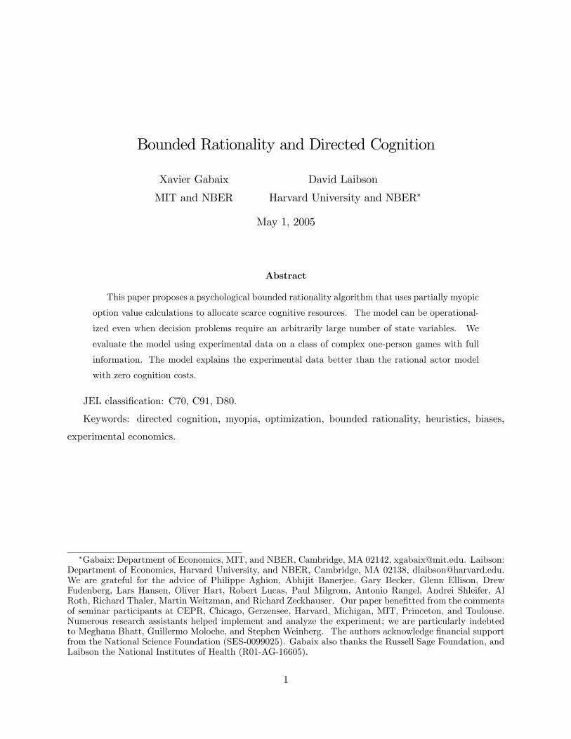
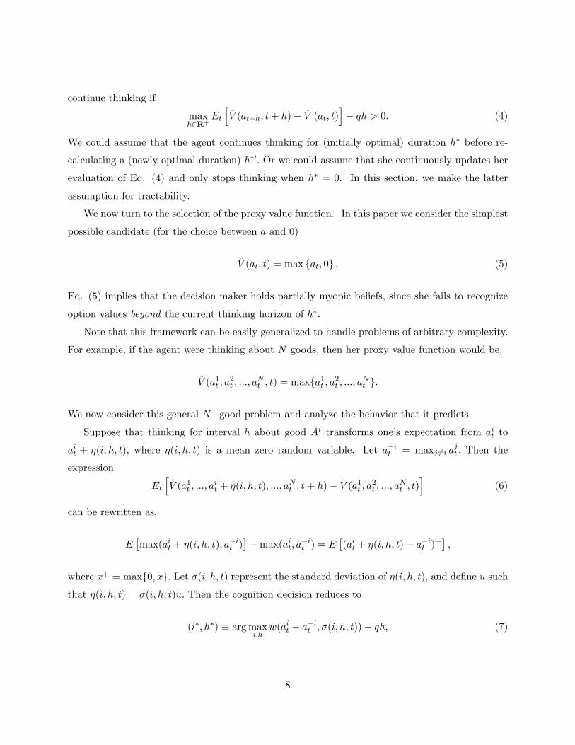
Figure 1: This Figure plots the expected bene�t from continued search � w; de�ned in Eq. 11� when the di¤erence between the value of the searched alternative and its best alternative is a,and the standard deviation of the information gained is � = 1: This w function is homogeneous ofdegree one.

where

v (a; �) = E�(a+ �u)+

�(8)

w (a; �) = v(a; �)� a+: (9)

When thinking generates Gaussian increments to knowledge u, we can write,

v(a; �) = a��a�

�+ ��

�a�

�: (10)

w(a; �) = �jaj���jaj�

�+ ��

�a�

�: (11)

where � and � = �0 are respectively the cumulative distribution and the density of a standard

Gaussian. Figure 1 shows w.

Our boundedly rational agents won�t necessarily use the �true�distribution of the information

shocks u. Our agent may use simpli�ed versions of it. Hence, we also consider the symmetric

distribution with atoms at �1. For this special case, which we denote with the superscript 0, we

9

get,

v0(a; �) =

8<: 12(a+ �) if jaj � �a+ if jaj > �

(12)

w0(a; �) =1

2(� � jaj)+: (13)

The simple, linear form above makes w0 convenient to use.

Let us apply this to our Brownian problem with at = a0 +R t0 � (s) dzs. Thinking for h more

minutes will reveal an amount of normally distributed information with standard deviation

�(t; h) =

�Z t+h

t�2(s)ds

�1=2:

The strategy in the directed cognition model is to continue thinking i¤ there is a h > 0 such that

w (at; �(t; h))� qh > 0:

This leads to the policy �continue i¤ jatj < at�, where at is implicitly de�ned by6

suph�0

w (at; �(t; h))� qh = 0: (14)

For the standard case of the directed cognition model (i.e., normally distributed information inno-

vations, so that w is de�ned in Eq. 11), at is de�ned by

suph�0

�at��� at�(t; h)

�+ ��

�at

�(t; h)

�� qh = 0:

For the case with atoms of information at�1 (w0 is de�ned in Eq. 13) at is de�ned by suph�0w0 (at; �(t; h))�qh = 0, so that

at = suph�0

�(t; h)� 2qh:

This contrasts with the policy of rational cognition, which maximizes (3). Finding the threshold

policy is typically much more complex and requires backward induction with a free boundary (i.e.,

solving a di¤erential equation with boundary conditions). The complexity of rational cognition

6Limiting oneself to very small h would lead an agent to always stop if at 6= 0, as limh!0 w (at; �(t; h)) =h�q = �qif at 6= 0. Hence, the decision maker is not so myopic that he can only look at the immediate future.

10

explodes when the number of state variables increases. This is the curse of dimensionality.

2.4 Comparing directed cognition to rational cognition

We can now compare directed cognition to rational cognition. We start with the special case in

which �2(t) = �2, so �2(t; h) = h�2: We call this the constant variance case. Appendix A also

provides a closed form solution for the case in which the variance falls linearly with time until the

variance hits zero � the a¢ ne variance case.

Proposition 1 For the constant variance case the value function is independent of t, and the

stopping rule is �stop i¤ jatj � a = ��2

q �. For rational cognition � = 1=4. For directed cognition

with normally distributed innovations, � is the solution of maxh�0w��;ph�� h = 0 (so � '

0:1012).7 For the directed cognition model with atoms at �1; � = 1=8:

The proof is in Appendix A. This Proposition implies that rational cognition and directed

cognition have the same comparative statics with respect to the variables of interest (the quantity

of information learned by unit of time, �2, and the �ow cost of thinking, q). But directed cognition

will stop thinking earlier, as its threshold is proportional to 0:1012, while rational cognition�s

threshold is 1=4.

The next Proposition characterizes the consequences of these policies. This Proposition presents

the true (objective) payo¤ expectations generated by stopping rules indexed by �: Recall that the

stopping threshold is given by a = ��2

q : Also, note that time-independence of the decision process

allows us to drop the t-subscripts from each of the expressions.

Proposition 2 Using the notation from Proposition 1, for both rational cognition and directed

cognition, the expected consumption utility is:

C(a) = E[a+� jat = a] =

8>><>>:0 if a � �a12

���2 + aq

�if �a < a < a

a if a � a

(15)

7There is a semi-explicit formula for �. If � ' 0:6210 is the solution of 2�� (��) = � (�), then an exact expressionfor � ' 0:1012 is � = �� (�) =2.

11

the decision maker will, on average, keep thinking about the problem for an amount of time:

T (a) = E[� � tjat = a] =

8<: 0 if jaj � a�a2=�2 + �2�2=q2 if jaj < a

(16)

and the value function V (a) = C (a)� qT (a) is:

V (a) = E�a+� � q (� � t) jat = a

�=

8>><>>:0 if a � �a�(12 � �)

�2

q +a2 +

q�2a2 if �a < a < a

a if a � a

(17)

The proof is in Appendix A.

Eq. (17) � the value function � allows us to compare the economic performance of the

algorithms. This value function depends on �; which is su¢ cient to characterize the stopping rules

of the algorithms (cf. Proposition 1).

Proposition 2 also decomposes payo¤s into their two subcomponents: payo¤s arising from con-

sumption utility8 � C(a) = E[a+� ja] � and costs arising from cognition costs � q E[� � tja]: Theintegrated measure of economic performance is the value function V = E [a+� � q (� � t) ja], whichis the expected consumption utility net of cognition costs.

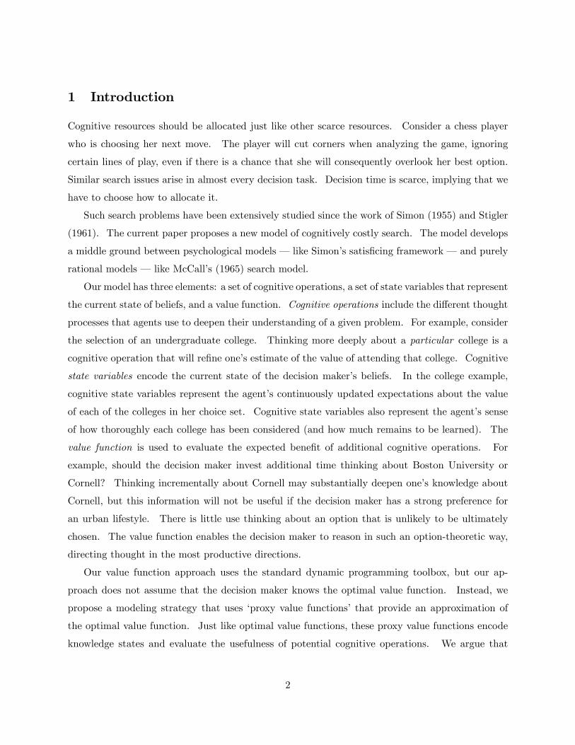
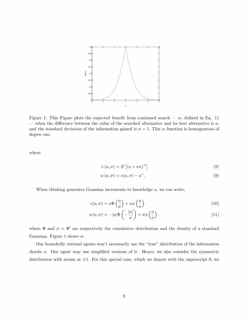
Proposition 2 enables us to plot (Figure 2) the value function under the three di¤erent cases:

rational cognition (solid line, � = 1=4), directed cognition with atomic information (� = 1=8,

dashed line), and directed cognition with Gaussian information (� = 0:1012, dot-dashed line). By

de�nition, the value function generated by rational cognition lies above the other two (suboptimal)

value functions. The three curves are compared in Figure 2.

This simple case allows us to study the relative performance of the algorithms in a case where

we can calculate the values in simple closed forms. Appendix A derives closed form solutions for

the a¢ ne variance case: �2 (t) = A � Bt. We can also derive more general results. We turn tothem now.

8When the consumer stops thinking, at time � , he will pick the good i¤ a� � 0, so his consumption utility will bea+� .

12

­0.4 ­0.3 ­0.2 ­0.1 0 0.1 0.2 0.3 0.40

0.05

0.1

0.15

0.2

0.25

0.3

0.35

0.4

a

V(a

)

Rational Cognition

Directed Cognition (atomic)

Directed Cognition (normal)

Figure 2: This Figure plots three objective value functions. We plot a on the horizontal axis andvalue functions on the vertical axis. We do this for three di¤erent policies: divine cognition (solidline, � = 1=4), directed cognition with atomic information (� = 1=8, dashed line), and directedcognition with Gaussian information (� = 0:1012, dotted line). The three curves are close toeach other (in the sense that the maximum di¤erence between the values is 0.022), which meansthat directed cognition has a perfomance close to that of divine cognition. The values come fromPropositions 1 and 2.

13

2.5 Quantitative relationship between the value functions of divine and directed

cognition

We can formalize the normative gap between divine and directed cognition by bounding the distance

between their respective value functions. We analyze the leading case of monotonically declining

variance functions.

The following Proposition bounds the gap between the true (objective) payo¤s generated by the

optimal stopping rule and the true (objective) payo¤s generated by the directed cognition stopping

rule. The Proposition is expressed in terms of �subjective value functions,�which can be shown to

bound the objective value functions. Such subjective value functions represent the expected utility

outcomes under the mistaken assumption that the current cognitive operation (with incremental

stopping time �) is the �nal cognitive operation. The subjective value functions are therefore based

on static beliefs, which counterfactually assume that there will be no future cognitive operations.

Such subjective value functions are relatively easy to calculate because they assume deterministic

stopping times. By contrast, optimal value functions incorporate optimally chosen stopping times

that depend on future realizations of random variables.

Proposition 3 Let V (x) represent the objective value function under the optimal policy (divine

cognition). Let V 1 represent the objective value function under the directed cognition policy. So V

and V 1 are the true expected payo¤s associated with the optimal policy and the directed cognition

policy. Suppose the variance function, � (�) = (� (t))t�0, is deterministic and weakly decreasing.9

Then,

S0�x;p2=�� (�)

�� S1 (x; � (�)) � V 1 (x; � (�)) � V (x; � (�)) � S2 (x; � (�)) � :::

::: � S0 (x; � (�)) + min(jxj; S0(0; � (�)))=2 (18)

where Si is the subjective value function,

Si(x; � (�)) = suph2R+

vi

x;

�Z h

0�2(s)ds

�1=2!� qh;

v0 is de�ned in (12), v1 is de�ned in (10), and v2(x; k) =�x+

px2 + k2

�=2.

9The nonincreasing � implies that �high payo¤� cognitive operations are done �rst. Hence, thinking displaysdecreasing returns over time.

14

Proposition 3 is proved in Appendix A.

Proposition 3 implies that the objective value functions for divine cognition (V ) and directed

cognition (V 1) are bounded below by S1 and above by S2: S1 represents the subjective value func-

tion associated with Gaussian innovations. S2 represents the subjective value function associated

with the density f2(u) =�2(1 + u2)3=2

��1.

It is useful to evaluate the bounds at the point x = 0, as this is where the option value V (x)�x+

is greatest. V (0; � (�)) gives the order of magnitude of the option value.

Proposition 4

V�0;p2=�� (�)

�� V 1 (0; � (�)) � V (0; � (�)) : (19)

This Proposition gives us a way of comparing the directed cognition model (with objective

value function V 1) to the optimal policy function (with objective value function V ). The di¤erence

between V 1 and V is bounded by the di¤erence between the value function V generated by standard

deviationp2=�� � 0:8� and the value function V generated by standard deviation �. Thus, the

directed cognition model performs as well as an optimal policy rule in a problem with payo¤s scaled

down by factorp2=� = 0:8.10 This holds for one dimensional problems �results for cases with

more dimensions are harder to derive.

Comparative statics analysis also implies that our directed cognition model is �close� to the

divine cognition model. The subjective and objective value functions are all increasing in �(�) anddecreasing in q. They also share other properties. All of the value functions tend to x+ as jxj ! 1;rise with x; have slope 1/2 at 0; and are symmetric around 0 (e.g., V (x)� x+ is even).

This section has described our directed cognition model. We were able to compare it to the

divine cognition model for a special case in which the decision maker chooses between A and 0.11

For this extremely simple example, the divine cognition approach is well-de�ned and solvable in

practice. In most problems of interest, the divine cognition model will not be of any use, since

economists can�t solve dynamic programming problems with a su¢ ciently large number of state

variables. Below, we turn to an example of such a problem. Speci�cally, this problem involves the

analysis of 10�10 (or 10�5) decision trees. Compared to real-world decision problems, such treesare not particularly complex. However, even simple decision trees like these generate hundreds of10Note that this scaling argument only applies at a = 0: For comparisons that apply at all values of a; refer back

to Proposition 3.11All of the bounding results in this subsection assume that the decision maker selects among two options (n = 2).

We can show that the lower bounds that we derive generalize to the case n � 3: Obtaining analogous upper boundsfor the general case remains an open question.

15

cognitive state variables. Divine cognition is useless here. But directed cognition, with its proxy

value function, can be applied without di¢ culty. We now turn to this application.

3 An experimental implementation of the directed cognition model

3.1 Decision trees

We use the directed cognition model to predict how experimental subjects will make choices in

complex decision trees. We analyze decision trees, since trees can be used to represent a wide class

of problems. We describe our decision trees at the beginning of this section, and then apply the

model to the analysis of these trees.

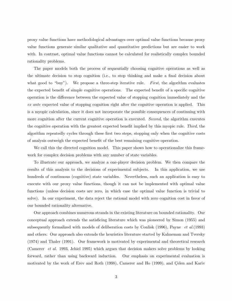
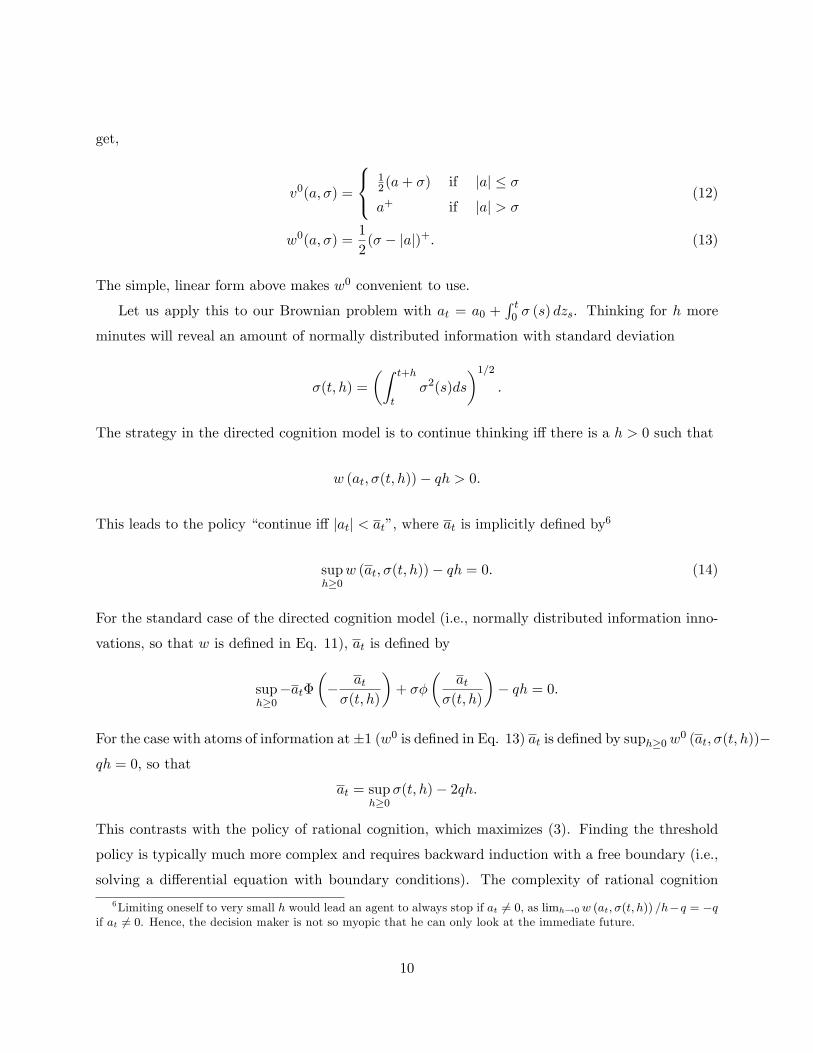
Consider the decision tree in Figure 3, which is one of twelve randomly generated trees that

we asked experimental subjects to analyze. Each starting box in the left-hand column leads

probabilistically to boxes in the second column. Branches connect boxes and each branch is

associated with a given probability.

For example, the �rst box in the last row contains a 5. From this box there are two branches

with respective probabilities 0.65 and 0.35. The numbers inside the boxes represent �ow payo¤s.

Starting from the box in the �rst column of the last row, there exist 7,776 possible outcome

paths. For example, the outcome path that follows the highest probability branch at each node is

h5; 4; 4; 3; 1;�2; 5; 5;�3; 4i. Integrating with appropriate probability weights over all 7,776 paths,the expected payo¤ of starting from the �rst box in the last row is 4.12.

Formally, we de�ne an outcome path as a feasible sequence of boxes that begins in column 1

and ends in the last (right-most) column. We de�ne the expected value of a starting row as the

probability-weighted value of all outcome paths that begin at a particular box in the left-most

column of the tree.

We asked undergraduate subjects to choose one of the boxes in the �rst column of Figure 3.

We told the subjects that they would be paid the expected value associated with whatever box

they chose. What box would you choose?

To clarify exposition, we will refer to the �nal choice of a starting row as the �consumption

choice.� This observable choice represents a subject�s response in the experiment. The subject

16

b c d ea f jg h i

0.2

5.1

5.2 .0

7.3

3

0 3 1 4.4

5.5 .0

5

5.7

5.2

4.0

1

1 ­5.8

5.0

1.0

3.0

1.1

­1 5.6

5.3

5

2.0

5.9

5

2.1

5.0

1.1

4.7

­2.0

5.8

5.0

5.0

5

­1.5

5.4

5

0 1.3 .1

5.3 .1 .1

5

­2.0

1.7

5.2

4

5.2

5.1

4.2

5.0

1.3

5

4.1

5.5 .2 .1

5

­5.0

1.6

5.3 .0

1.0

3

­2.0

5.2 .7

5

­4.1

5.5 .2 .1

5

­4 5.5 .5

­2.2

5.7 .0

5

1.9

5.0

1.0

4

­3.7

5.2

5

4.3 .0

5.6

5

­5.0

3.0

1.0

1.9

5

­4.7 .0

4.2

5.0

1

­3.1 .9

0.5 .4 .1

1 1.1

5.0

4.8 .0

1

4.8

5.1

5

­4 0.3

3.6

7

3.2

5.1 .6

5

3 1

­2.5

5.0

5.3 .0

5.0

5

­2.6

5.0

5.1 .2

4.0

1.0

3.0

1.1

5.8

­7.0

5.6 .2 .0

5.1

3.3

5.0

1.1

5.1

4.3

5

­8.4

9.5 .0

1

­5 3.0

1.3 .0

3.0

1.6

5

1.1

5.4

5.0

5.3 .0

5

­4.5

2.3

3.1 .0

5

­2.6 .4

­2.0

5.0

5.0

7.3

3.5

0 ­1.4 .6

3.8

5.0

1.0

3.0

1.1

3.0

1.0

1.1

8.8

­2.9

5.0

5

­4.7

5.2

5

­1.0

5.9 .0

5

­1

­1 13.1

5.8

5

­5.8

5.0

5.0

9.0

1

3 ­5.6 .0

7.3

3

5.1 .5

5.1 .1 .1

5

3.1

5.7

5.1

­5.0

1.2 .7

9

­1.1 .7

5.1

5

0.2

5.5 .2

5

­2.3

3.6

7

­4.2

5.4 .0

5.2 .1

­5.3

3.1

5.5

2

5.1

5.0

5.2 .6

5.6 .2

5.1

4.0

1

­1.6

6.2

9.0

5

2 ­6 0 ­1.3

3.6

7

2.1

5.3

3.0

1.0

1.5

­5.4

5.5

5

3.1 .8 .0

4.0

5.0

1

­3 ­5.2

5.5

5.2

3 2.3 .3 .4

­4.2

5.2 .0

5.5

­4 5.6

5.3

5

0 2 0 4 1 ­2 4 ­3 ­1 5

Figure 3: This Figure reproduces one of our 12 randomly-generated games. Each starting boxin the left-hand column leads probabilistically to boxes in the second column. Branches connectboxes and each branch is associated with a given probability. For example, the �rst box in thelast row contains a 5. From this box there are two branches with respective probabilities 0.65 and0.35. The numbers inside the boxes represent �ow payo¤s. Starting from the last row, there exist7,776 outcome paths. For example, the outcome path that follows the highest probability branchat each node is h5; 4; 4; 3; 1;�2; 5; 5;�3; 4i. We asked undergraduate subjects to guess which of theboxes a; :::; j in the �rst column of this Figure had the highest expected payo¤. Which one wouldyou pick?

17

also makes many �cognition choices�that guide her internal thought processes. We jointly model

consumption and cognition choices, and then test the model with the observed consumption choices.

3.2 Application of the directed cognition model

The directed cognition model can be used to analyze trees like those in Figure 3. We describe such

an application of the model in this subsection.12

Our application uses a basic cognitive operation: extending a partially examined path one

column deeper into the tree. Such extensions enable the decision maker to improve her forecast of

the expected value of a particular starting row.

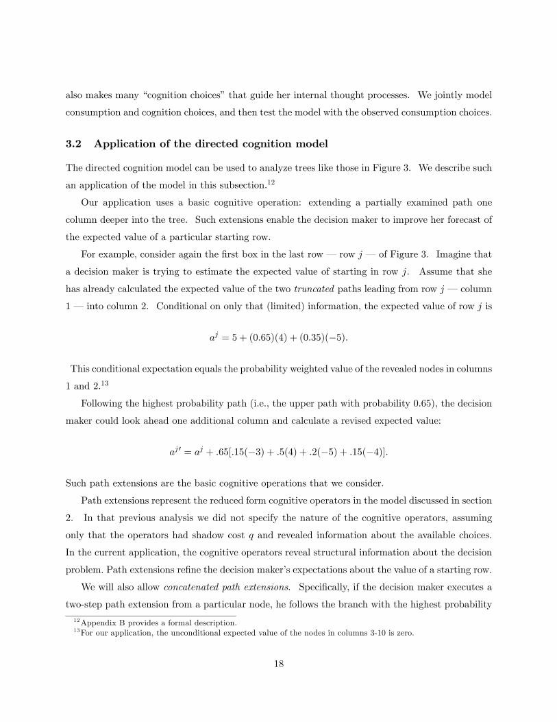
For example, consider again the �rst box in the last row � row j � of Figure 3. Imagine that

a decision maker is trying to estimate the expected value of starting in row j. Assume that she

has already calculated the expected value of the two truncated paths leading from row j � column

1 � into column 2. Conditional on only that (limited) information, the expected value of row j is

aj = 5 + (0:65)(4) + (0:35)(�5):

This conditional expectation equals the probability weighted value of the revealed nodes in columns

1 and 2.13

Following the highest probability path (i.e., the upper path with probability 0.65), the decision

maker could look ahead one additional column and calculate a revised expected value:

aj 0 = aj + :65[:15(�3) + :5(4) + :2(�5) + :15(�4)]:

Such path extensions are the basic cognitive operations that we consider.

Path extensions represent the reduced form cognitive operators in the model discussed in section

2. In that previous analysis we did not specify the nature of the cognitive operators, assuming

only that the operators had shadow cost q and revealed information about the available choices.

In the current application, the cognitive operators reveal structural information about the decision

problem. Path extensions re�ne the decision maker�s expectations about the value of a starting row.

We will also allow concatenated path extensions. Speci�cally, if the decision maker executes a

two-step path extension from a particular node, he follows the branch with the highest probability

12Appendix B provides a formal description.13For our application, the unconditional expected value of the nodes in columns 3-10 is zero.

18

for two steps deeper into the tree. Hence, starting from the last row of Figure 3, his updated

estimate would be,

aj 00 = aj 0 + (:65)(:5)[:3(0) + :05(3) + :65(3)]:

Such concatenated path extensions generalize naturally. An h-step path extension looks h columns

more deeply into the tree. At each node along this path the extension follows the branch with

highest probability.

A multi-column explored path originating from a node in column 1 can be extended in many

ways, since an explored path may contain numerous nodes that that have unexplored branches.

Let f represent a feasible path extension; f embeds information about the starting row of the path

that will be extended, the speci�c previously explored node from which the new extension will

originate, and the number of steps of the new extension (e.g., starting at a previously explored

node, proceed h columns deeper into the tree by starting with a particular branch originating at

that node; for the remaining h� 1 steps, always follow the branch with highest probability).Let �f represent the standard deviation of the updated estimate resulting from application of

f . Hence,

�2f = E(f(ai(f))� ai(f))2;

where i(f) represents the starting row which begins the path that f extends, ai(f) represents the

initial estimate of the value of row i(f), and f(ai(f)) represents the updated value resulting from

the path extension.

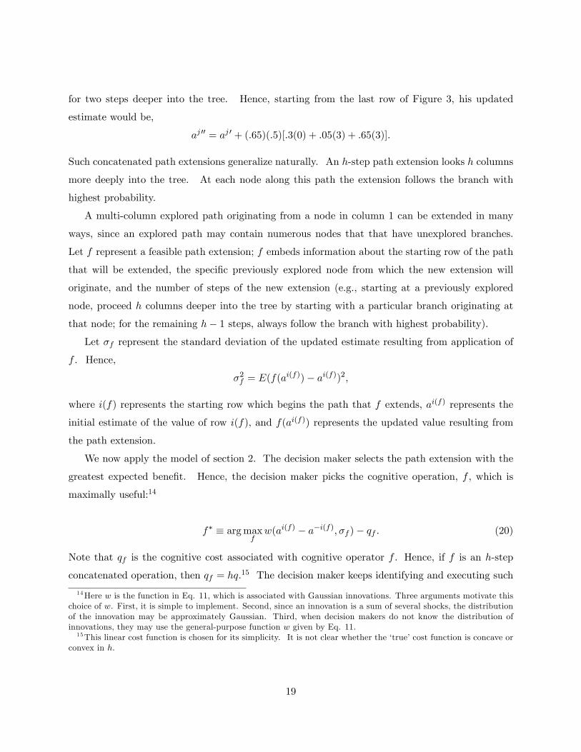
We now apply the model of section 2. The decision maker selects the path extension with the

greatest expected bene�t. Hence, the decision maker picks the cognitive operation, f , which is

maximally useful:14

f� � argmaxfw(ai(f) � a�i(f); �f )� qf : (20)

Note that qf is the cognitive cost associated with cognitive operator f . Hence, if f is an h-step

concatenated operation, then qf = hq.15 The decision maker keeps identifying and executing such

14Here w is the function in Eq. 11, which is associated with Gaussian innovations. Three arguments motivate thischoice of w. First, it is simple to implement. Second, since an innovation is a sum of several shocks, the distributionof the innovation may be approximately Gaussian. Third, when decision makers do not know the distribution ofinnovations, they may use the general-purpose function w given by Eq. 11.15This linear cost function is chosen for its simplicity. It is not clear whether the �true�cost function is concave or

convex in h:

19

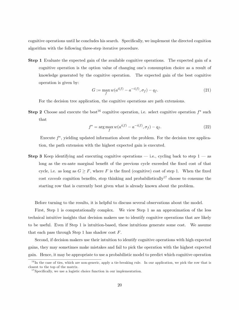
cognitive operations until he concludes his search. Speci�cally, we implement the directed cognition

algorithm with the following three-step iterative procedure.

Step 1 Evaluate the expected gain of the available cognitive operations. The expected gain of a

cognitive operation is the option value of changing one�s consumption choice as a result of

knowledge generated by the cognitive operation. The expected gain of the best cognitive

operation is given by:

G := maxfw(ai(f) � a�i(f); �f )� qf : (21)

For the decision tree application, the cognitive operations are path extensions.

Step 2 Choose and execute the best16 cognitive operation, i.e. select cognitive operation f� such

that

f� = argmaxfw(ai(f) � a�i(f); �f )� qf : (22)

Execute f�; yielding updated information about the problem. For the decision tree applica-

tion, the path extension with the highest expected gain is executed.

Step 3 Keep identifying and executing cognitive operations � i.e., cycling back to step 1 � as

long as the ex-ante marginal bene�t of the previous cycle exceeded the �xed cost of that

cycle, i.e. as long as G � F , where F is the �xed (cognitive) cost of step 1. When the �xedcost exceeds cognition bene�ts, stop thinking and probabilistically17 choose to consume the

starting row that is currently best given what is already known about the problem.

Before turning to the results, it is helpful to discuss several observations about the model.

First, Step 1 is computationally complex. We view Step 1 as an approximation of the less

technical intuitive insights that decision makers use to identify cognitive operations that are likely

to be useful. Even if Step 1 is intuition-based, these intuitions generate some cost. We assume

that each pass through Step 1 has shadow cost F .

Second, if decision makers use their intuition to identify cognitive operations with high expected

gains, they may sometimes make mistakes and fail to pick the operation with the highest expected

gain. Hence, it may be appropriate to use a probabilistic model to predict which cognitive operation

16 In the case of ties, which are non-generic, apply a tie-breaking rule. In our application, we pick the row that isclosest to the top of the matrix.17Speci�cally, we use a logistic choice function in our implementation.

20

the decision maker will execute in Step 2. However, we overlook this issue in the current paper and

assume that the decision maker always selects the cognitive operation with the highest expected

gain.

Third, in the decision tree application we use rational expectations to calculate � and aj ,18 but

many other approaches are sensible. For example, �2 could be estimated using past observations

of (f(ai(f))� ai(f))2.Fourth, we assume that Step 3 is backward looking. Speci�cally, the decision maker uses past

information about the expected gains of cognitive operators to determine whether it is worth paying

cost F to generate a new set of intuitions. No doubt this treatment could be improved in several

ways. But, consistent with our modeling strategy, we choose the simplest approach that is broadly

in accord with the psychology and the �cognitive economics�of the task.

Fifth, if Figure 3 contained a box with an extremely large payo¤ (e.g. 100), that box would no

doubt draw the attention of subjects. To capture this e¤ect, we could add another mental operator:

global scanning. For example, �Scan the tree. Look for the box with the largest unexplored positive

or negative payo¤. Determine how much this box a¤ects the estimated value of each row.� A

rigorous de�nition for global scanning is easy to formulate though such a de�nition is notationally

cumbersome. We did not include global scanning in our set of mental operators to keep the model

as simple as possible, and also because the stochastic structure we use to generate decision trees

does not generate outlier boxes.

To sum up, the directed cognition algorithm executes the path extension with the highest

expected value net of cognition cost, q. The algorithm continues in this way � evaluating the

expected value of path extensions and executing the most promising path extension � until no

remaining path extension has a positive expected value net of cognition cost.

This procedure radically simpli�es analysis of our decision trees. Each unsimpli�ed tree has

approximately 100,000 paths leading from the �rst column to the last column. Our directed

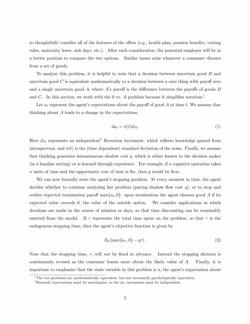
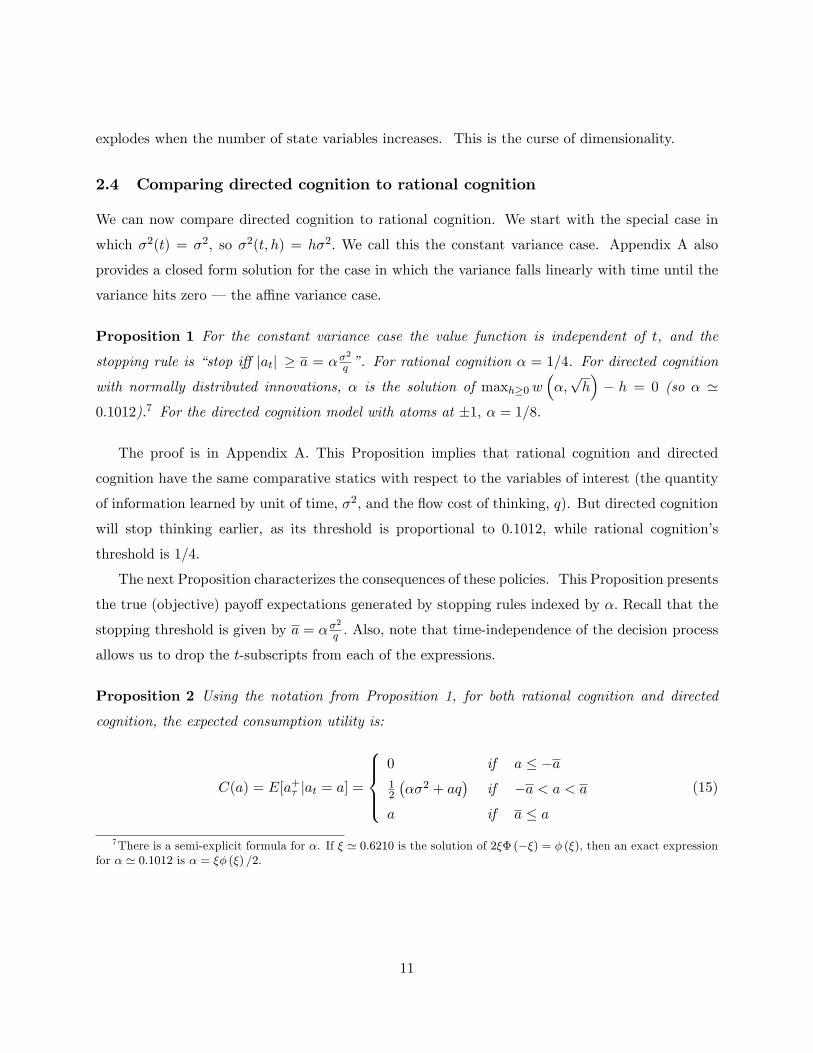
cognition algorithm restricts attention to only a handful of these paths. For example, Figure 4

plots the path extensions generated by the directed cognition model for the game in Figure 3.

Using option-theoretic considerations, the directed cognition algorithm restricts analysis to 7100;000

of the possible paths in this tree. After these seven path extensions are examined, the algorithm

18To justify the use of rational expectations in estimating � and aj , our experimental design allows the decisionmaker to scan the entire tree and form an estimate of the branching structure and the distribution of node values.

21

b c d ea f jg h i

0.2

5.1

5.2 .0

7.3

3

0 3 1 4.4

5.5 .0

5

5.7

5.2

4.0

1

1 ­5.8

5.0

1.0

3.0

1.1

­1 5.6

5.3

5

2.0

5.9

5

2.1

5.0

1.1

4.7

­2.0

5.8

5.0

5.0

5

­1.5

5.4

5

0 1.3 .1

5.3 .1 .1

5

­2.0

1.7

5.2

4

5.2

5.1

4.2

5.0

1.3

5

4.1

5.5 .2 .1

5

­5.0

1.6

5.3 .0

1.0

3

­2.0

5.2 .7

5

­4.1

5.5 .2 .1

5

­4 5.5 .5

­2.2

5.7 .0

5

1.9

5.0

1.0

4

­3.7

5.2

5

4.3 .0

5.6

5

­5.0

3.0

1.0

1.9

5

­4.7 .0

4.2

5.0

1

­3.1 .9

0.5 .4 .1

1 1.1

5.0

4.8 .0

1

4.8

5.1

5

­4 0.3

3.6

7

3.2

5.1 .6

5

3 1

­2.5

5.0

5.3 .0

5.0

5

­2.6

5.0

5.1 .2

4.0

1.0

3.0

1.1

5.8

­7.0

5.6 .2 .0

5.1

3.3

5.0

1.1

5.1

4.3

5

­8.4

9.5 .0

1

­5 3.0

1.3 .0

3.0

1.6

5

1.1

5.4

5.0

5.3 .0

5

­4.5

2.3

3.1 .0

5

­2.6 .4

­2.0

5.0

5.0

7.3

3.5

0 ­1.4 .6

3.8

5.0

1.0

3.0

1.1

3.0

1.0

1.1

8.8

­2.9

5.0

5

­4.7

5.2

5

­1.0

5.9 .0

5

­1

­1 13.1

5.8

5

­5.8

5.0

5.0

9.0

1

3 ­5.6 .0

7.3

3

5.1 .5

5.1 .1 .1

5

3.1

5.7

5.1

­5.0

1.2 .7

9

­1.1 .7

5.1

5

0.2

5.5 .2

5

­2.3

3.6

7

­4.2

5.4 .0

5.2 .1

­5.3

3.1

5.5

2

5.1

5.0

5.2 .6

5.6 .2

5.1

4.0

1

­1.6

6.2

9.0

5

2 ­6 0 ­1.3

3.6

7

2.1

5.3

3.0

1.0

1.5

­5.4

5.5

5

3.1 .8 .0

4.0

5.0

1

­3 ­5.2

5.5

5.2

3 2.3 .3 .4

­4.2

5.2 .0

5.5

­4 5.6

5.3

5

0 2 0 4 1 ­2 4 ­3 ­1 5

Figure 4: In the game presented in Figure 3 the directed cognition model looked at only 7 paths outof approximately 100,000 paths. This Figure highlights those 7 paths (including 1 path extension).The algorithm was very frugal. Table 1 compares the row choices implied by directed cognition tothe row choices actually made by our subjects.

22

stops. Option value calculations enable the decision maker to simplify his problem by restricting

attention to a tiny fraction of the available information.

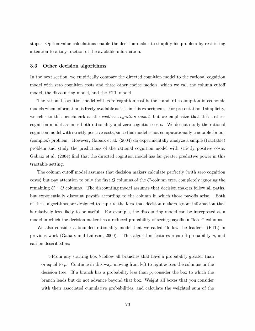
3.3 Other decision algorithms

In the next section, we empirically compare the directed cognition model to the rational cognition

model with zero cognition costs and three other choice models, which we call the column cuto¤

model, the discounting model, and the FTL model.

The rational cognition model with zero cognition cost is the standard assumption in economic

models when information is freely available as it is in this experiment. For presentational simplicity,

we refer to this benchmark as the costless cognition model, but we emphasize that this costless

cognition model assumes both rationality and zero cognition costs. We do not study the rational

cognition model with strictly positive costs, since this model is not computationally tractable for our

(complex) problem. However, Gabaix et al. (2004) do experimentally analyze a simple (tractable)

problem and study the predictions of the rational cognition model with strictly positive costs.

Gabaix et al. (2004) �nd that the directed cognition model has far greater predictive power in this

tractable setting.

The column cuto¤ model assumes that decision makers calculate perfectly (with zero cognition

costs) but pay attention to only the �rst Q columns of the C-column tree, completely ignoring the

remaining C �Q columns. The discounting model assumes that decision makers follow all paths,but exponentially discount payo¤s according to the column in which those payo¤s arise. Both

of these algorithms are designed to capture the idea that decision makers ignore information that

is relatively less likely to be useful. For example, the discounting model can be interpreted as a

model in which the decision maker has a reduced probability of seeing payo¤s in �later�columns.

We also consider a bounded rationality model that we called �follow the leaders� (FTL) in

previous work (Gabaix and Laibson, 2000). This algorithm features a cuto¤ probability p, and

can be described as:

>From any starting box b follow all branches that have a probability greater than

or equal to p. Continue in this way, moving from left to right across the columns in the

decision tree. If a branch has a probability less than p, consider the box to which the

branch leads but do not advance beyond that box. Weight all boxes that you consider

with their associated cumulative probabilities, and calculate the weighted sum of the

23

boxes.

This heuristic describes the FTL value of a starting box b: In our econometric analysis, we

estimate p = 0:30; costless cognition corresponds to p = 0.

More precisely, we take the average payo¤s over trajectories starting from box b, with the

transition probabilities indicated on the branches, but with the additional rule that the trajectory

stops if the last transition probability has been < p.19 For example, consider the following FTL

(p = 0:60) calculation for row b in Figure 3. FTL follows all paths that originate in row b, stopping

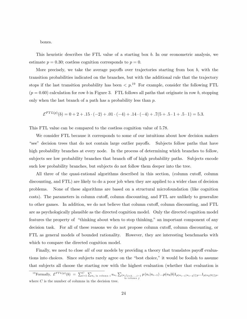
only when the last branch of a path has a probability less than p.

EFTL(p)(b) = 0 + 2 + :15 � (�2) + :01 � (�4) + :14 � (�4) + :7(5 + :5 � 1 + :5 � 1) = 5:3:

This FTL value can be compared to the costless cognition value of 5.78:

We consider FTL because it corresponds to some of our intuitions about how decision makers

�see� decision trees that do not contain large outlier payo¤s. Subjects follow paths that have

high probability branches at every node. In the process of determining which branches to follow,

subjects see low probability branches that branch o¤ of high probability paths. Subjects encode

such low probability branches, but subjects do not follow them deeper into the tree.

All three of the quasi-rational algorithms described in this section, (column cuto¤, column

discounting, and FTL) are likely to do a poor job when they are applied to a wider class of decision

problems. None of these algorithms are based on a structural microfoundation (like cognition

costs). The parameters in column cuto¤, column discounting, and FTL are unlikely to generalize

to other games. In addition, we do not believe that column cuto¤, column discounting, and FTL

are as psychologically plausible as the directed cognition model. Only the directed cognition model

features the property of �thinking about when to stop thinking,�an important component of any

decision task. For all of these reasons we do not propose column cuto¤, column discounting, or

FTL as general models of bounded rationality. However, they are interesting benchmarks with

which to compare the directed cognition model.

Finally, we need to close all of our models by providing a theory that translates payo¤ evalua-

tions into choices. Since subjects rarely agree on the �best choice,�it would be foolish to assume

that subjects all choose the starting row with the highest evaluation (whether that evaluation is

19Formally, EFTL(p)(b) =PC

i=1

Pni in column i

uniP

(nj)j=2;:::;i�1in column j

p (nijni�1) :::p(n2jb)1p(ni�1jni�2)�p:::1p(n2jb)�p,

where C is the number of columns in the decision tree.

24

rational or quasi-rational). Instead, we assume that actions with the highest evaluations will be

chosen with the greatest frequency. Formally, we choose a logit speci�cation, which is the most

common modeling device for these purposes. Speci�cally, assume that there are B possible choices

with evaluations fE1; E2; : : : ; EBg given by one of the candidate models. Then the probability ofpicking box b is given by:

Pb =exp(�Eb)PBb0=1 exp(�Eb0)

: (23)

We estimate the nuisance parameter � in our econometric analysis.

3.4 The details of the experimental design

We tested the model using experimental data from 259 subjects recruited from the general Harvard

undergraduate population.20 Subjects were guaranteed a minimum payment of $7 and could receive

more if they performed well. They received an average payment of $20.08.

3.4.1 Decision Trees

The experiment was based around twelve randomly generated trees, one of which is reproduced

in Figure 3. We chose large trees because we wanted undergraduates to use heuristics to �solve�

these problems. Half of the trees have 10 rows and 5 columns of payo¤ boxes; the other half of

the trees are 10 � 10. The branching structure which exits from each box was chosen randomly

and is i.i.d. across boxes within each tree. The distributions that we used and the twelve resulting

trees themselves are presented in an accompanying working paper. On average the twelve trees

have approximately three exit branches per box (excluding the boxes in the last column of each

tree which have no exit branches).

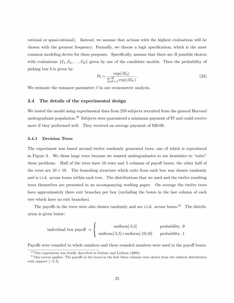
The payo¤s in the trees were also chosen randomly and are i.i.d. across boxes.21 The distrib-

ution is given below:

individual box payo¤ =

8<: uniform[-5,5] probability .9

uniform[-5,5]+uniform[-10,10] probability .1

Payo¤s were rounded to whole numbers and these rounded numbers were used in the payo¤ boxes.

20This experiment was brie�y described in Gabaix and Laibson (2003).21One caveat applies. The payo¤s in the boxes in the �rst three columns were drawn from the uniform distribution

with support [�5; 5].

25

Experimental instructions (available on the authors�web pages) described the concept of ex-

pected value to the subjects. Subjects were told to choose one starting row from each of the twelve

trees. Subjects were told that one of the trees would be randomly selected and that they would

be paid the true expected value for the starting box that they chose in that tree. Subjects were

given a maximal time of 40 minutes to read the experimental instructions and make all twelve of

their choices. We analyzed data only from the 251 subjects who made a choice in all of the twelve

decision trees.

3.4.2 Debrie�ng form and expected value calculations

After passing in their completed tree forms, subjects �lled out a debrie�ng form which asked them

to �describe how [they] approached the problem of �nding the best starting boxes in the 12 games.�

Subjects were also asked for background information (e.g., major and math/statistics/economics

background). Subjects were then asked to make 14 expected value calculations in simple trees

(three 2�2 trees , three 2�3 trees, and one 2�4 tree). Subjects were told to estimate the expectedvalue of each starting row in these trees. Figure 5 provides an example of one such tree. Subjects

were told that they would be given a �xed reward (� $1:25) for every expected value that they

calculated correctly (i.e., within 10% of the exact answer). We gave subjects these expected

value questions because we wanted to identify any subjects who did not understand the concept

of expected value. We exclude any subject from our econometric analysis who did not answer

correctly at least half of the fourteen expected value questions. Out of the 251 subjects who

provided an answer for all twelve decision trees, 230, or 92%, correctly answered at least half of the

fourteen expected value questions. Out of this subpopulation, the median score was 12 out of 14

correct; 190 out of 230 answered at least one of the two expected values in Figure 5 correctly.

4 Experimental results

We restrict analysis to the 230 subjects who met our inclusion criteria22, but the results are almost

identical when we include all 251 subjects who completed the decision trees.

Had subjects chosen randomly, they would have chosen starting boxes with an average payo¤

22They chose a row in all twelve decision trees and answered correctly at least half of the expected value questionson the post-experiment debrie�ng form.

26

Figure 5: This Figure presents a representative game from the debrie�ng quiz. The answer for boxk is: 4 + :3 (�2 + :9 � 5 + :1 � 2) + :7 (3 + :25 � 5 + :75 � 2) = 8: 835. Theses games allow us to testthat subjects understand well the concept of expected value. Out of the 251 subjects who providedan answer for all twelve decision trees, 230, or 92%, correctly answered at least half of the fourteenexpected value questions. Out of this subpopulation, the median score was 12 out of 14 correct.

of $1.30.23 Had the subjects chosen the starting boxes with the highest payo¤, the average chosen

payo¤ would have been $9.74. In fact, subjects chose starting boxes with average payo¤ $6.72.

We are interested in comparing �ve di¤erent classes of models: costless cognition, directed

cognition, column cuto¤, discounting, and FTL. All of these models have a nuisance parameter, �;

which captures the tendency to pick starting boxes with the highest evaluations (see Eq. 23). For

each model, we estimate a di¤erent � parameter. Directed cognition, column cuto¤, discounting,

and FTL also require an additional parameter which we estimate in our econometric analysis.

4.1 The Euclidean distance Lm between a model m and the data

We call bPbg the fraction of subjects playing game g who chose box b. Say that a model m (costless

cognition, directed cognition, FTL etc.) assigns the value Embg to box b in game g. Following

standard practice in the discrete choice literature, we parameterize the link between this value and

the probability that a player will choose b in game g by

Pmbg (�) = exp(�Embg )=BXb0=1

exp(�Emb0g) (24)

for a given �. To determine �, we minimize the Euclidean distance kPm(�) � bPk between theempirical distribution bP and the distribution predicted by the model, Pm(�). If we optimize over23 In expectation this would have been zero since our games were randomly drawn from a distribution with zero

mean. Our realized value is well within the two-standard error bands.

27

�, we get the distance:

Lm� bP� = min

�2R+kPm(�)� bPk (25)

Those are the distances we report in Table 2.

4.2 Empirical results

For the directed cognition model we estimate q = 0:012, implying that the shadow price of extending

a path one-column deeper into the tree is a little above 1 cent. We can translate this estimate

into real time processing speed. Given a cost q and the directed cognition algorithm, people will

make Ng(q) elementary operations in game g (g 2 f1; :::; 12g): Say that people need � seconds perelementary mental operation: for instance, extending a path 3 columns ahead and updating the

point estimate of a box accordingly takes 3� seconds. Then the total time spent on the experiment

is: T (q) = �P12g=1Ng(q): Given that our subjects had roughly 35 minutes (40 minutes total minus

roughly 5 minutes to read the instructions), we can infer from our calibrated value of q = 0:012 the

value of � = (35 minutes) =�P12

g=1Ng(q)�= 2:2 seconds per box. We view both of these numbers

as reasonable. We had chosen 1 cent per box and 1 second per box as our preferred values before

we estimated these values.

For the column-cuto¤ model, we estimate Q = 8; implying that the decision maker evaluates

only the �rst 8 columns of each tree (and hence all of the columns in 10 � 5 trees). For the

column-discounting model we estimate � = 0:91; implying that the probability that the decision

maker sees a payo¤ in column c is (:91)c : Finally, for FTL we estimate p = 0:30, implying that the

decision maker follows branches until she encounters a branch probability which is less than .30.

We had exogenously imposed a p value of 0.25 in our previous work (Gabaix and Laibson, 2000).

< Insert Table 1 here >

The �rst panel (Values) in Table 1 presents the predictions of our models for the sample game

in Figure 3. �Values�plots the row values estimated by each of the models. Using these estimated

values and a logistic transformation (24) generates choice probabilities, which are reported in the

second panel of the Table.

Directed cognition estimated that row j has the highest value (the estimate is 7.19). Our

subjects apparently reached the same conclusion since more of them chose row j (36.5%, see the

empirical probabilities) than any other row. By contrast, row f actually has the highest value (6.88,

28

see the costless cognition values). Hence directed cognition failed to pick the optimal box. This is

a desirable result, since directed cognition makes the same �mistake�as our subjects. As Figure

4 shows, directed cognition overlooks the fact that row j has many overlooked paths that lead to

negative payo¤s.

The sample game analyzed in Table 1 is just one of our 12 games. To gain a complete picture

of our results we now turn to Table 2, which reports test statistics derived from the data from all

12 games. The rows of the Table represent the di¤erent models, m 2 fcostless cognition, directedcognition, column-cuto¤, column-discounting, FTLg. Column 1 reports distance metric bLm; whichmeasures the distance between the estimated model and the empirical data. A small distance bLmindicates a good �t between model and data. Columns 2-5 report the di¤erences bLm � bLm0

; and

the associated asymptotic standard errors. When bLm � bLm0> 0; model m performs relatively

poorly, since the distance of model m from the empirical data (bLm) is greater than the distance ofthe model m0 from the empirical data (bLm0

).

<Insert Table 2 here.>

As column 2 of Table 2 shows, all of the decision cost models beat costless cognition. The di¤er-

ences between the distance measures are: bLcostless cognition�bLdirected cognition = 0:399, bLcostless cognition�bLcolumn cuto¤ = 0:221, bLcostless cognition � bLcolumn discounting = 0:190, and bLcostless cognition � bLFTL =0:488. All of these di¤erences have associated t-statistics of at least 5.

Among the decision cost models the two winners are directed cognition and FTL. Both of

these models dominate column cuto¤ and column discounting. The di¤erence between directed

cognition and FTL is not statistically signi�cant. The general success of the directed cognition

model is somewhat surprising, since column cuto¤, column discounting, and FTL were designed

explicitly for this game against nature, whereas directed cognition is a more generally applicable

algorithm.

5 Conclusion

We have proposed an algorithm for boundedly rational choice. The model provides a theory of

cognitive resource allocation and is tractable even in highly complex environments. We empirically

evaluate the model in such a setting. Developing models of decision-making that can be practically

applied to complex problems is an important research frontier.

29

The directed cognition model is modular and there are many improvements that could be made

to each of its parts: expanding the set of mental operators, improving the sophistication of the

myopic proxy value function, adding trembles in the choice of the best cognitive operation, etc. In

general, we have adopted the simplest possible version of each of the model�s features.

We wish to highlight several shortcomings of the model. First, the implementation of the

model requires the researcher to specify the set of cognitive operators. Ideally, a more general

model would internally generate these cognitive operators. Second, the model only captures a few

of the simplifying short-cuts that decision makers adopt. Third, the model does not exploit the fact

that people often �solve� hard problems by developing specialized heuristics for those problems.

To paraphrase Tolstoy, rational models are all rational in the same way, but boundedly rational

models are all di¤erent. A unifying framework for bounded rationality represents a formidable

research challenge.

30

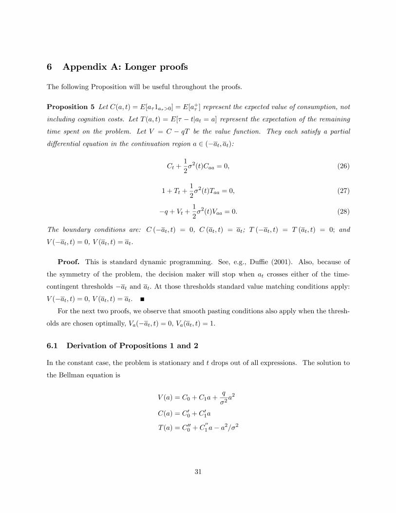
6 Appendix A: Longer proofs

The following Proposition will be useful throughout the proofs.

Proposition 5 Let C(a; t) = E[a�1a�>0] = E[a+� ] represent the expected value of consumption, not

including cognition costs. Let T (a; t) = E[� � tjat = a] represent the expectation of the remainingtime spent on the problem. Let V = C � qT be the value function. They each satisfy a partial

di¤erential equation in the continuation region a 2 (�at; at):

Ct +1

2�2(t)Caa = 0; (26)

1 + Tt +1

2�2(t)Taa = 0; (27)

�q + Vt +1

2�2(t)Vaa = 0: (28)

The boundary conditions are: C (�at; t) = 0, C (at; t) = at; T (�at; t) = T (at; t) = 0; and

V (�at; t) = 0, V (at; t) = at.

Proof. This is standard dynamic programming. See, e.g., Du¢ e (2001). Also, because of

the symmetry of the problem, the decision maker will stop when at crosses either of the time-

contingent thresholds �at and at: At those thresholds standard value matching conditions apply:V (�at; t) = 0, V (at; t) = at.

For the next two proofs, we observe that smooth pasting conditions also apply when the thresh-

olds are chosen optimally, Va(�at; t) = 0; Va(at; t) = 1:

6.1 Derivation of Propositions 1 and 2

In the constant case, the problem is stationary and t drops out of all expressions. The solution to

the Bellman equation is

V (a) = C0 + C1a+q

�2a2

C(a) = C 00 + C01a

T (a) = C 000 + C001 a� a2=�2

31

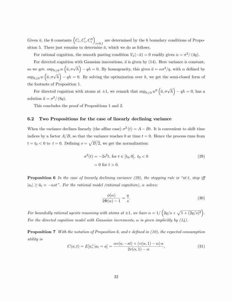
Given a, the 6 constants�Ci; C

0i ; C

00i

�i=0;1

are determined by the 6 boundary conditions of Propo-

sition 5. There just remains to determine a, which we do as follows.

For rational cognition, the smooth pasting condition Va(�a) = 0 readily gives � = �2= (4q).For directed cognition with Gaussian innovations, a is given by (14). Here variance is constant,

so we get: suph�0w�a; �

ph�� qh = 0. By homogeneity, this gives a = ��2=q, with � de�ned by

suph�0w�a; �

ph�� qh = 0. By solving the optimization over h, we get the semi-closed form of

the footnote of Proposition 1.

For directed cognition with atoms at �1, we remark that suph�0w0�a; �

ph�� qh = 0, has a

solution a = �2= (8q).

This concludes the proof of Propositions 1 and 2.

6.2 Two Propositions for the case of linearly declining variance

When the variance declines linearly (the a¢ ne case) �2 (t) = A�Bt. It is convenient to shift timeindices by a factor A=B, so that the variance reaches 0 at time t = 0. Hence the process runs from

t = t0 < 0 to t = 0. De�ning s =pB=2, we get the normalization:

�2(t) = �2s2t, for t 2 [t0; 0]; t0 < 0 (29)

= 0 for t > 0.

Proposition 6 In the case of linearly declining variance (29), the stopping rule is �at t, stop i¤

jatj � at = ��st�. For the rational model (rational cognition), � solves:

�(�)

2�(�)� 1 =q

s: (30)

For boundedly rational agents reasoning with atoms at �1, we have � = 1=�2q=s+

p1 + (2q=s)2

�.

For the directed cognition model with Gaussian increments, � is given implicitly by (14).

Proposition 7 With the notation of Proposition 6, and v de�ned in (10), the expected consumption

utility is

C(a; t) = E[a+� jat = a] =�v(a;�st) + (v(�; 1)� �) a

2v(�; 1)� � ; (31)

32

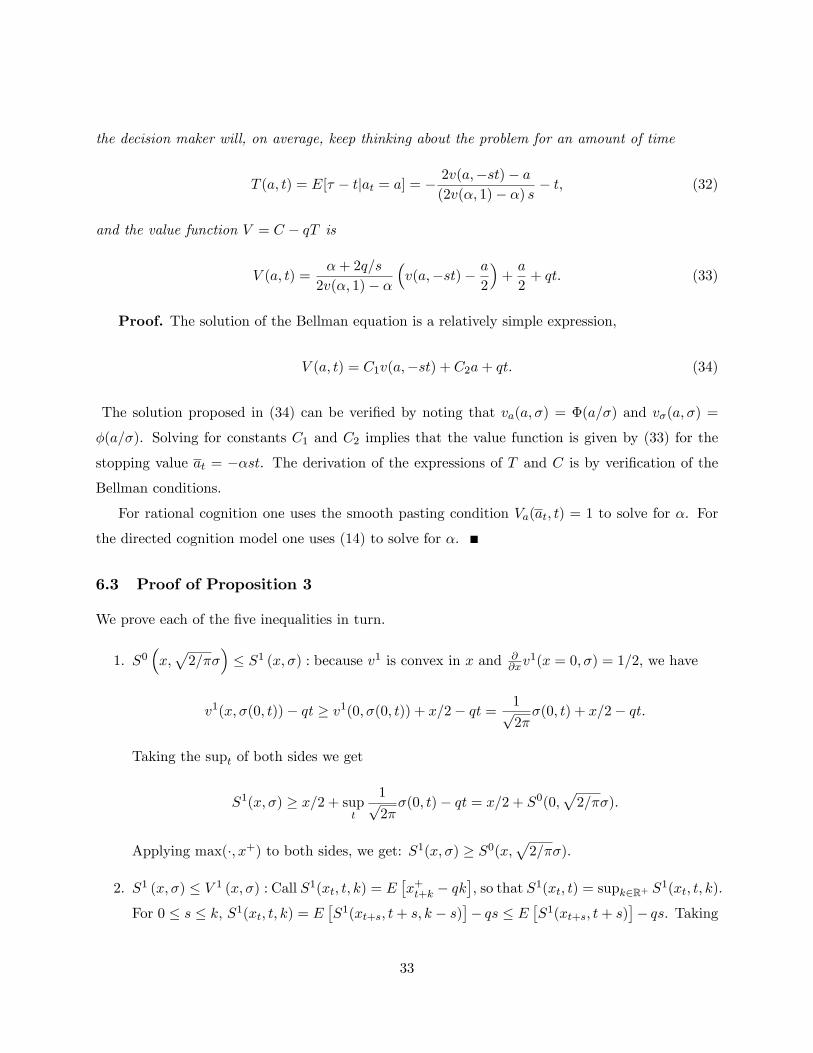
the decision maker will, on average, keep thinking about the problem for an amount of time

T (a; t) = E[� � tjat = a] = �2v(a;�st)� a(2v(�; 1)� �) s � t; (32)

and the value function V = C � qT is

V (a; t) =�+ 2q=s

2v(�; 1)� �

�v(a;�st)� a

2

�+a

2+ qt: (33)

Proof. The solution of the Bellman equation is a relatively simple expression,

V (a; t) = C1v(a;�st) + C2a+ qt: (34)

The solution proposed in (34) can be veri�ed by noting that va(a; �) = �(a=�) and v�(a; �) =

�(a=�). Solving for constants C1 and C2 implies that the value function is given by (33) for the

stopping value at = ��st. The derivation of the expressions of T and C is by veri�cation of the

Bellman conditions.

For rational cognition one uses the smooth pasting condition Va(at; t) = 1 to solve for �. For

the directed cognition model one uses (14) to solve for �.

6.3 Proof of Proposition 3

We prove each of the �ve inequalities in turn.

1. S0�x;p2=��

�� S1 (x; �) : because v1 is convex in x and @

@xv1(x = 0; �) = 1=2, we have

v1(x; �(0; t))� qt � v1(0; �(0; t)) + x=2� qt = 1p2��(0; t) + x=2� qt:

Taking the supt of both sides we get

S1(x; �) � x=2 + supt

1p2��(0; t)� qt = x=2 + S0(0;

p2=��):

Applying max(�; x+) to both sides, we get: S1(x; �) � S0(x;p2=��):

2. S1 (x; �) � V 1 (x; �) : Call S1(xt; t; k) = E�x+t+k � qk

�, so that S1(xt; t) = supk2R+ S

1(xt; t; k).

For 0 � s � k, S1(xt; t; k) = E�S1(xt+s; t+ s; k � s)

�� qs � E

�S1(xt+s; t+ s)

�� qs. Taking

33

the supk2R+ on the left-hand side, we get S1(xt; t) � E�S1(xt+s; t+ s)

�� qs for s small

enough: As V 1(xt; t) = E�V 1(xt+s; t+ s)

�� qs, we get, for D1(xt; t) = V 1(xt; t) � S1(xt; t),

that D1(xt; t) � E�D1(xt+s; t+ s)

�, i.e. D1 is a submartingale. The search process stops

at a random time T , and then S1(xT ; T ) = V 1(xT ; T ) = x+T , so D1(xT ; T ) = 0. As

D1(xt; t) � E�D1(xT ; T )

�= 0, we can conclude V 1(xt; t) � S1(xt; t):

3. V 1 (x; � (�)) � V (x; � (�)) : this is immediate because this holds for any policy vi, as V is the

best possible policy.

4. First, observe (with, again, x0 = x)

E[max(x� ; 0)] = E[x�=2 + jx� j=2] by the identity max(b; 0) = (b+ jbj)=2

= x=2 + E[jx� j]=2 as xt is a martingale which stops almost surely

� x=2 + E[x2� ]1=2=2

= x=2 + (x2 + E[�(0; t)2])1=2=2 as x2t � �(0; t)2 is a martingale (35)

� x=2 + (x2 + �(0;m)2)1=2=2 with m = E [� jx0 = x] as �2(0; t) is concave

so we get: V (x) � x=2 + (x2 +m)1=2=2� qm. Given that

S2(x; �) = x=2 + supt2R+

(x2 + �(0; t)2)1=2=2� qt

we get V (x) � S2 (x).

5. We use the fact that for non-negative a; b,pa+ b �

pa+

pb :

x=2 +px2 + �2(0; t)=2� qt �

�x+

px2�=2 + �(0; t)=2� qt = x+ + �(0; t)=2� qt

so by taking the supt of both sides we get: S2(x; �) � x++S0(0; �), whose right-hand side is

less than or equal to S0(x; �) +min(jxj; S0(0; �))=2 by direct veri�cation using the de�nitionof v0.

34

6.4 Proof of Proposition 4

We apply x = 0 to (18) and get

S0�0;p2=�� (�)

�� V 1 (0; � (�)) � V (0; � (�)) � S0 (x; � (�)) :

Applying that inequality top2=�� (�) rather than � (�), we get

S0�0;�p

2=��2� (�)

�� V 1

�0;p2=�� (�)

�� V

�0;p2=�� (�)

�� S0

�x;p2=�� (�)

�:

Putting those two inequalities together, we extract

V�0;p2=�� (�)

�� S0

�x;p2=�� (�)

�� V 1 (0; � (�)) � V (0; � (�)) ;

which allows us to conclude.

6.5 Derivation of the standard errors of distance measures

There are G = 12 games, B = 10 starting boxes per game, and I = 230 subjects who satisfy our

inclusion criterion. Call Xi 2 RBG the choice vector such that Xibg = 1 if subject i played box b

at game g, and 0 otherwise. Call P = E[Xi] the true distribution of choices, bP :=PIi=1X

i=I the

empirical distribution of choices. We call � = E[XiXi0]�PP 0 the (BG�BG) variance-covariancematrix of the choices Xi, and its estimator b� := (

PIi=1X

iXi0=I � bP bP 0)=(1 � 1=I). We take theEuclidean norm kPk =

Pg

�Pb P

2bg

�1=2for P 2 RBG. We call Lm

� bP ; �� = kPm(�)� bPk so thatbLm = min� Lm � bP ; �� is the empirical distance between the model and the data. Call Lm and �mthe analogues for the true distribution of choices, i.e. Lm = min� kPm(�)�Pk. We also set b�m :=argmin�2R+ L

m� bP ; ��.

We now derive statistics24 on bLm. " := bP � P has a distribution such thatpI" � N(0;�) for

large I 0s. Because " = O�I�1=2

�is small, Lm

� bP� = Lm (P ) + @PLm (P ) � " + O(1=I). By the

envelope theorem, @PLm (P ) = �m, where:

�mbg =� bPbg � Pmbg (�m)�

Xb0

� bPb0g � Pmb0g(�m)�2!�1=2

: (36)

24We use the fact, exploited by Vuong (1989) and Hansen-Heaton-Luttmer (1995), that we do not have to explicitlyderive the distribution of b�m to get the distribution of bLm.

35

So we get the representation formula

bLm = Lm +�m � "+O (1=I) : (37)

Suppose that �m 6= 0, i.e. the model m is misspeci�ed (this will be the case for all the models

considered 25). Eq. (37) implies thatpI(bLm � Lm) � N(0;�m0��m), and gives us a consistent

estimator of the standard deviation on bLm,b�Lm = �d�m0b�d�m=I�1=2 : (38)

We will be interested in the di¤erence Lm � Ln of the performance of two theories m and n.

Eq. (37) implies that bLm � bLn = Lm � Ln + (�m ��n) � " + O (1=I). Hence we get a consistentestimator of the standard deviation of bLm � bLm0

,

b�Lm�Ln = �(d�m � c�n)0b�(d�m � c�n)=I�1=2 : (39)

Those formulae carry over to models that have been optimized. Our models have a free parame-

ter: in directed cognition, the parameter is q, the cost (per box) of cognition; in column-discounting,

it is �, the discount rate; in column cuto¤, it is Q, the �nal column analyzed; in FTL it is p, the

cuto¤ probability. In general, we parametrize a class of models M with a real (or vector) parame-

ter x: M = fM (x) ; x 2 XMg. For instance, if M = FTL, and x = 0:25, then M(x) represents

FTL with probability cuto¤ p = 0:25, and the space of parameter x is XFTL = [0; 1]. The space

can be discrete: for M = Column Cuto¤; XM = f1; 2; :::; 10g: For each x, M(x) gives a vectorof values EM (x) for the boxes, and hence a distance to the empirical distribution, for a given � :jjP�EM (x); �

�� bP jj.

For model M , we can optimize over parameter x to �nd the best possible �t by calculatingbLM := minx2XM min�2R+ jjP�EM (x); �

�� bP jj. As this is again an application of the delta method,

the standard errors calculated in (38) and (39) are still valid even though we optimize on parameter

x.25A test that Lm 6= 0 can be readily performed using the estimates bLm and b�Lm given in the tables.

36

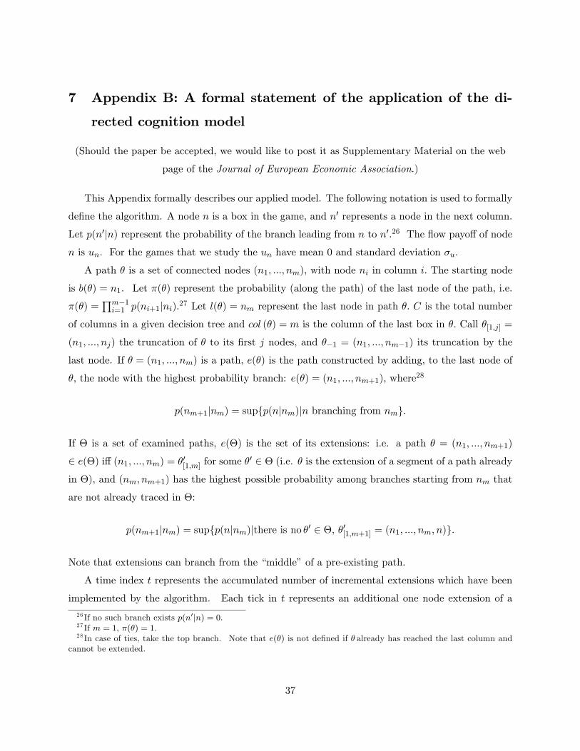
7 Appendix B: A formal statement of the application of the di-

rected cognition model

(Should the paper be accepted, we would like to post it as Supplementary Material on the web

page of the Journal of European Economic Association.)

This Appendix formally describes our applied model. The following notation is used to formally

de�ne the algorithm. A node n is a box in the game, and n0 represents a node in the next column.

Let p(n0jn) represent the probability of the branch leading from n to n0:26 The �ow payo¤ of node

n is un: For the games that we study the un have mean 0 and standard deviation �u:

A path � is a set of connected nodes (n1; :::; nm), with node ni in column i: The starting node

is b(�) = n1. Let �(�) represent the probability (along the path) of the last node of the path, i.e.

�(�) =Qm�1i=1 p(ni+1jni):27 Let l(�) = nm represent the last node in path �: C is the total number

of columns in a given decision tree and col (�) = m is the column of the last box in �: Call �[1;j] =

(n1; :::; nj) the truncation of � to its �rst j nodes, and ��1 = (n1; :::; nm�1) its truncation by the

last node. If � = (n1; :::; nm) is a path, e(�) is the path constructed by adding, to the last node of

�; the node with the highest probability branch: e(�) = (n1; :::; nm+1), where28

p(nm+1jnm) = supfp(njnm)jn branching from nmg:

If � is a set of examined paths, e(�) is the set of its extensions: i.e. a path � = (n1; :::; nm+1)

2 e(�) i¤ (n1; :::; nm) = �0[1;m] for some �0 2 � (i.e. � is the extension of a segment of a path already

in �), and (nm; nm+1) has the highest possible probability among branches starting from nm that

are not already traced in �:

p(nm+1jnm) = supfp(njnm)jthere is no �0 2 �, �0[1;m+1] = (n1; :::; nm; n)g:

Note that extensions can branch from the �middle�of a pre-existing path.

A time index t represents the accumulated number of incremental extensions which have been

implemented by the algorithm. Each tick in t represents an additional one node extension of a

26 If no such branch exists p(n0jn) = 0.27 If m = 1; �(�) = 1:28 In case of ties, take the top branch. Note that e(�) is not de�ned if � already has reached the last column and

cannot be extended.

37

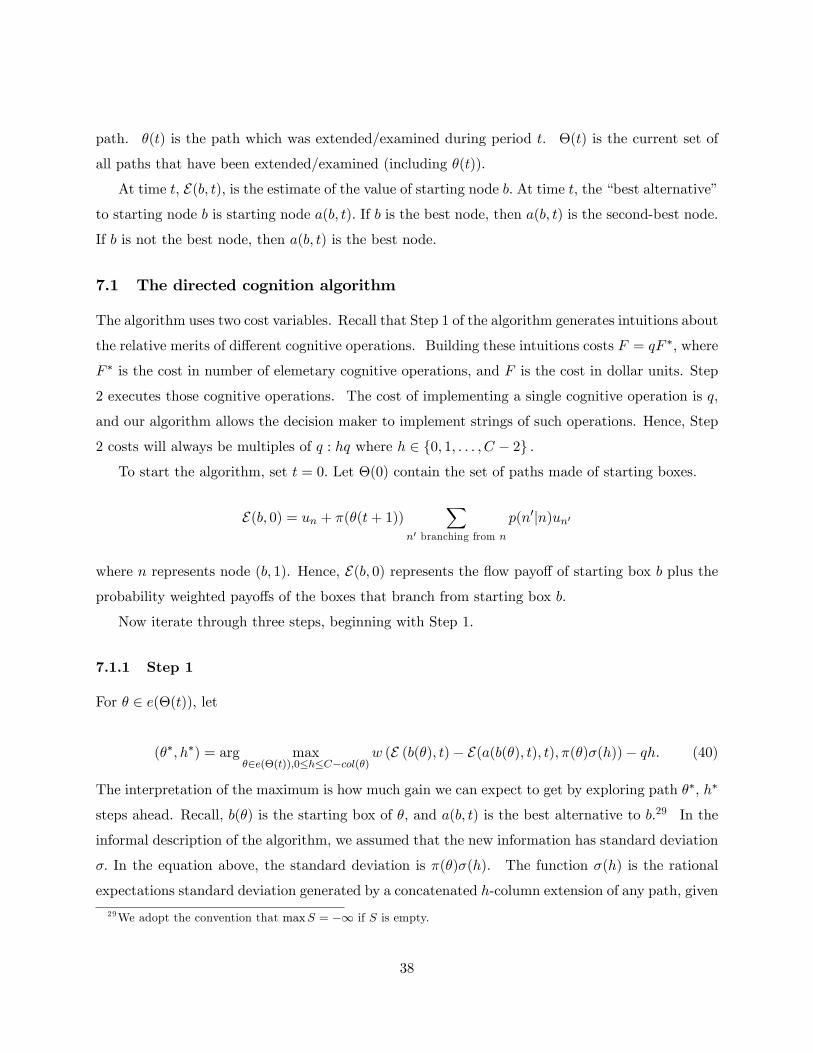
path. �(t) is the path which was extended/examined during period t. �(t) is the current set of

all paths that have been extended/examined (including �(t)).

At time t, E(b; t), is the estimate of the value of starting node b: At time t, the �best alternative�to starting node b is starting node a(b; t): If b is the best node, then a(b; t) is the second-best node.

If b is not the best node, then a(b; t) is the best node.

7.1 The directed cognition algorithm

The algorithm uses two cost variables. Recall that Step 1 of the algorithm generates intuitions about

the relative merits of di¤erent cognitive operations. Building these intuitions costs F = qF �, where

F � is the cost in number of elemetary cognitive operations, and F is the cost in dollar units. Step

2 executes those cognitive operations. The cost of implementing a single cognitive operation is q,

and our algorithm allows the decision maker to implement strings of such operations. Hence, Step

2 costs will always be multiples of q : hq where h 2 f0; 1; : : : ; C � 2g :To start the algorithm, set t = 0: Let �(0) contain the set of paths made of starting boxes.

E(b; 0) = un + �(�(t+ 1))X

n0 branching from n

p(n0jn)un0

where n represents node (b; 1). Hence, E(b; 0) represents the �ow payo¤ of starting box b plus theprobability weighted payo¤s of the boxes that branch from starting box b.

Now iterate through three steps, beginning with Step 1.

7.1.1 Step 1

For � 2 e(�(t)); let

(��; h�) = arg max�2e(�(t));0�h�C�col(�)

w (E (b(�); t)� E(a(b(�); t); t); �(�)�(h))� qh: (40)

The interpretation of the maximum is how much gain we can expect to get by exploring path ��, h�

steps ahead. Recall, b(�) is the starting box of �, and a(b; t) is the best alternative to b.29 In the

informal description of the algorithm, we assumed that the new information has standard deviation

�: In the equation above, the standard deviation is �(�)�(h). The function �(h) is the rational

expectations standard deviation generated by a concatenated h-column extension of any path, given

29We adopt the convention that maxS = �1 if S is empty.

38

that the probability of reaching the beginning of the extended portion of the path is unity. The

factor �(�) adjusts for the probability of actually reaching the extended portion of the path. Recall

that �(�) is the probability of reaching the last node of path �, i.e. �(�) =Qm�1i=1 p(ni+1jni): The

�(h) function is derived below, after Step 3.

Call G the value of the maximum in (40). Go to step 2.

7.1.2 Step 2

In this step we execute the (concatenated) cognitive operation with the highest expected gain. We

�explore path ��at depth h��. In detail:

i. If h� = 0, go directly to Step 3.

ii. Let �(t + 1) = ��: In the set of examined paths, add �(t + 1), and, if it is the extension of a

path �0 at its terminal node, remove that path:

�(t+ 1) := �(t) [ f�(t+ 1)gnf��1(t+ 1)g if ��1(t+ 1) 2 �(t)

:= �(t) [ f�(t+ 1)g otherwise.

iii. Update the value of the starting box b(�(t+1)): If b 6= b(�(t+1)); then set E(b; t+1) = E(b; t):If b = b(�(t+ 1)); then set

E(b; t+ 1) = E(b; t) + �(�(t+ 1))X

n0 branching from n

p(n0jn)un0 (41)

where n = l(�(t+ 1)):

iv. Set h� = h� � 1: Set t = t+ 1:

v. If h� � 1; set �(t+ 1) = e(�(t)) and set �� = e(�(t)): Then, go to substep ii above.

vi. If h� = 0, go to Step 3.

7.1.3 Step 3

i. If G � qF , go to Step 1.

ii. If G < qF , stop the search and select as choice node argmaxb2B E(b; t):

39

This ends the algorithm, but we have one remaining loose end. We still need to derive the

standard deviation function �(h):

7.2 The value of �(h)

For a generic draw of probabilities at a node n0, we have r(n0) branches and probabilities that

we can order: p1(n0) � ::: � pr(n0)(n0): They are random variables. Recall that �u represents the

standard deviation of the payo¤ in a box. Exploring one column ahead will give an expected square

value: �2(1) = �2uE[p21+ :::+p

2r ]. Exploring two steps ahead, following the highest probability path

between columns, gives: �2(2) = E[(p21+ :::+ p2r)�

2u+ p

21 � �2(1)] = (1+E[p21])�2(1). In general, for

h � 0: �2(h) = (1 + E[p21] + :::+ E[p21]h�1)�2(1) =1�E[p21]h1�E[p21]

�2(1).

8 References

Bernheim, Douglas and Antonio Rangel, �Addiction and Cue-Triggered Decision Processes�,

American Economic Review 94 (2004), 1558-1590.

Bertsekas, Dimitri P., and John N. Tsitsiklis, Neuro-Dynamic Programming. (Cambridge, MA:

Athena Scienti�c, 1996).

Camerer, Colin, Eric J. Johnson, Talia Rymon, and Sankar Sen, �Cognition and Framing in

Sequential Bargaining for Gains and Losses,�in Ken Binmore, Alan Kirman, and Piero Tani,

eds., Frontiers of game theory. (Cambridge, MA: MIT Press, 1993).

Camerer, Colin and Teck-Hua Ho, �Experience Weighted Attraction Learning in Normal-Form

Games,�Econometrica, 67 (1999), 827-874.

Çelen, Bo¼gaçhan and Shachar Kariv, �Distinguishing Informational Cascades from Herd Behavior

in the Laboratory,�94 (2004), American Economic Review, 484-498.

Conlisk, John, �Why Bounded Rationality?�Journal of Economic Literature, 34 (1996), 669-700.

Costa-Gomes, Miguel, Vincent Crawford, and Bruno Broseta, �Cognition and Behavior in Normal-

Form Games: An Experimental Study,�Econometrica, 69 (2001), 1193-1235.

D�Avolio, Gene and Eric Nierenberg, �Investor Attention: Evidence from the Message Boards,�

mimeo, Harvard, 2003.

40

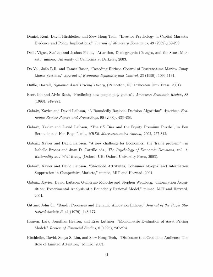
Daniel, Kent, David Hirshleifer, and Siew Hong Teoh, �Investor Psychology in Capital Markets:

Evidence and Policy Implications,�Journal of Monetary Economics, 49 (2002),139-209.

Della Vigna, Stefano and Joshua Pollet, �Attention, Demographic Changes, and the Stock Mar-

ket,�mimeo, University of California at Berkeley, 2003.

Do Val, João B.R. and Tamer Basar, �Receding Horizon Control of Discrete-time Markov Jump

Linear Systems,�Journal of Economic Dynamics and Control, 23 (1999), 1099-1131.

Du¢ e, Darrell, Dynamic Asset Pricing Theory, (Princeton, NJ: Princeton Univ Press, 2001).

Erev, Ido and Alvin Roth, �Predicting how people play games�. American Economic Review, 88

(1998), 848-881.

Gabaix, Xavier and David Laibson, �A Boundedly Rational Decision Algorithm�American Eco-

nomic Review Papers and Proceedings, 90 (2000), 433-438.

Gabaix, Xavier and David Laibson, �The 6D Bias and the Equity Premium Puzzle�, in Ben

Bernanke and Ken Rogo¤, eds., NBER Macroeconomics Annual, 2002, 257-312.

Gabaix, Xavier and David Laibson, �A new challenge for Economics: the �frame problem��, in

Isabelle Brocas and Juan D. Carrillo eds., The Psychology of Economic Decisions, vol. 1:

Rationality and Well-Being, (Oxford, UK: Oxford University Press, 2003).

Gabaix, Xavier and David Laibson, �Shrouded Attributes, Consumer Myopia, and Information

Suppression in Competitive Markets,�mimeo, MIT and Harvard, 2004.

Gabaix, Xavier, David Laibson, Guillermo Moloche and Stephen Weinberg, �Information Acqui-

sition: Experimental Analysis of a Boundedly Rational Model,�mimeo, MIT and Harvard,

2004.

Gittins, John C., �Bandit Processes and Dynamic Allocation Indices,�Journal of the Royal Sta-

tistical Society B, 41 (1979), 148-177.

Hansen, Lars, Jonathan Heaton, and Erzo Luttmer, �Econometric Evaluation of Asset Pricing

Models�Review of Financial Studies, 8 (1995), 237-274.

Hirshleifer, David, Sonya S. Lim, and Siew Hong Teoh, �Disclosure to a Credulous Audience: The

Role of Limited Attention,�Mimeo, 2003.

41

Jehiel, Philippe, �Limited Horizon Forecast in Repeated Alternate Games,�Journal of Economic

Theory, 67 (1995), 497-519.

Jehiel, Philippe, �Bounded Rationality and Imperfect Learning: Game Theory vs AI,� Greek

Economic Review, 2004

Jehiel, Philippe, �Analogy-Based Expectation Equilibrium,�Journal of Economic Theory, 2005.

Johnson, Eric J., Colin Camerer, Sanka Sen, and Talia Rymon, �Detecting Failures of Backward

Induction: Monitoring Information Search in Sequential Bargaining,� Journal of Economic

Theory, 104 (2002), 16-47.

Kahneman, Daniel and Amos Tversky, �Judgment Under Uncertainty: Heuristics and Biases,�

Science (1974), 1124-1131.

Lynch, Anthony, �Decision Frequency and Synchronization across Agents: Implications for Ag-

gregate Consumption and Equity Returns,�Journal of Finance, 51 (1996), 1479-98.

Mankiw, N. Gregory, and Ricardo Reis, �Sticky Information Versus Sticky Prices: a Proposal to

Replace the New Keynesian Phillips Curve,�Quarterly Journal of Economics, 117 (2002),

1295-1328.

McCall, John J., �The Economics of Information and Optimal Stopping Rules,�Journal of Busi-

ness, 38 (1965), 300-317.

Payne, John W., James R. Bettman, and Eric J. Johnson, The Adaptive Decision Maker, (Cam-

bridge, UK: Cambridge University Press, 1993).

Peng, Lin and Wei Xiong, �Capacity Constrained Learning and Asset Price Comovement,�mimeo,

Princeton, 2002.

Roberts, Kevin and Martin Weitzman, �On a General Approach to Search and Information Gath-

ering,�MIT Department of Economics Working Paper No. 263, 1980.

Simon, Herbert, �A Behavioral Model of Rational Choice,�Quarterly Journal of Economics, 69

(1955), 99-118.

Sims, Christopher, �Implications of Rational Inattention,� Journal of Monetary Economics, 50

(2003), 665-690.

42

Stigler, George, �The Economics of Information,�Journal of Political Economy, 69 (1961), 213-

225.

Thaler, Richard, Quasi Rational Economics, (New York, NY: Russell Sage, 1991).

Vuong, Quang H., �Likelihood ratio tests for model selection and non-tested hypotheses�, Econo-

metrica, 57 (1989), 307-33.

Weitzman, Martin, �Optimal search for the best alternative,�Econometrica 47 (1979), 641-54.

Woodford, Michael, �Imperfect Common Knowledge and the E¤ects of Monetary Policy,� in

Philippe Aghion, Roman Frydman, Joseph Stiglitz, and Michael Woodford, eds., Knowl-

edge, Information, and Expectations in Modern Macroeconomics: in Honor of Edmund S.

Phelps (Princeton, NJ: Princeton University Press, 2002).

43

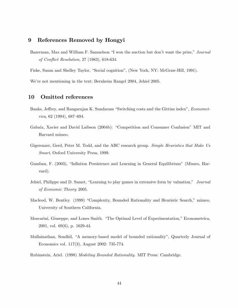
9 References Removed by Hongyi

Bazerman, Max and William F. Samuelson �I won the auction but don�t want the prize,�Journal

of Con�ict Resolution, 27 (1983), 618-634.

Fiske, Susan and Shelley Taylor, �Social cognition�, (New York, NY: McGraw-Hill, 1991).

We�re not mentioning in the text: Bernheim Rangel 2004, Jehiel 2005.

10 Omitted references

Banks, Je¤rey, and Rangarajan K. Sundaram �Switching costs and the Gittins index�, Economet-

rica, 62 (1994), 687�694.

Gabaix, Xavier and David Laibson (2004b): �Competition and Consumer Confusion�MIT and

Harvard mimeo.

Gigerenzer, Gerd, Peter M. Todd, and the ABC research group. Simple Heuristics that Make Us

Smart, Oxford University Press, 1999.

Gumbau, F. (2003), �In�ation Persistence and Learning in General Equilibrium� (Mimeo, Har-

vard).

Jehiel, Philippe and D. Samet, �Learning to play games in extensive form by valuation,� Journal

of Economic Theory 2005.

Macleod, W. Bentley. (1999) �Complexity, Bounded Rationality and Heuristic Search,�mimeo,

University of Southern California.

Moscarini, Giuseppe, and Lones Smith. �The Optimal Level of Experimentation,�Econometrica,

2001, vol. 69(6), p. 1629-44.

Mullainathan, Sendhil, �A memory-based model of bounded rationality�, Quarterly Journal of

Economics vol. 117(3), August 2002: 735-774.

Rubinstein, Ariel. (1998) Modeling Bounded Rationality. MIT Press: Cambridge.

44

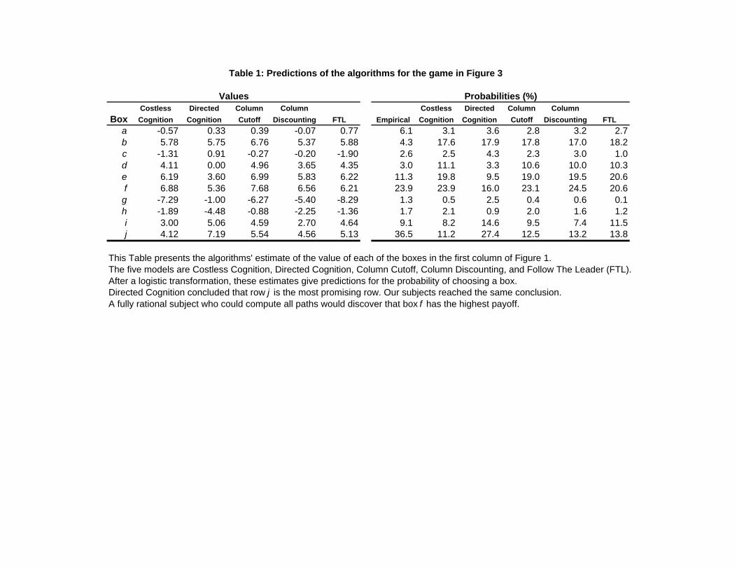
Table 1: Predictions of the algorithms for the game in Figure 3

Costless Directed Column Column Costless Directed Column ColumnBox Cognition Cognition Cutoff Discounting FTL Empirical Cognition Cognition Cutoff Discounting FTL

a -0.57 0.33 0.39 -0.07 0.77 6.1 3.1 3.6 2.8 3.2 2.7b 5.78 5.75 6.76 5.37 5.88 4.3 17.6 17.9 17.8 17.0 18.2c -1.31 0.91 -0.27 -0.20 -1.90 2.6 2.5 4.3 2.3 3.0 1.0d 4.11 0.00 4.96 3.65 4.35 3.0 11.1 3.3 10.6 10.0 10.3e 6.19 3.60 6.99 5.83 6.22 11.3 19.8 9.5 19.0 19.5 20.6f 6.88 5.36 7.68 6.56 6.21 23.9 23.9 16.0 23.1 24.5 20.6g -7.29 -1.00 -6.27 -5.40 -8.29 1.3 0.5 2.5 0.4 0.6 0.1h -1.89 -4.48 -0.88 -2.25 -1.36 1.7 2.1 0.9 2.0 1.6 1.2i 3.00 5.06 4.59 2.70 4.64 9.1 8.2 14.6 9.5 7.4 11.5j 4.12 7.19 5.54 4.56 5.13 36.5 11.2 27.4 12.5 13.2 13.8

This Table presents the algorithms' estimate of the value of each of the boxes in the first column of Figure 1. The five models are Costless Cognition, Directed Cognition, Column Cutoff, Column Discounting, and Follow The Leader (FTL).After a logistic transformation, these estimates give predictions for the probability of choosing a box.Directed Cognition concluded that row j is the most promising row. Our subjects reached the same conclusion.A fully rational subject who could compute all paths would discover that box f has the highest payoff.

Probabilities (%)Values

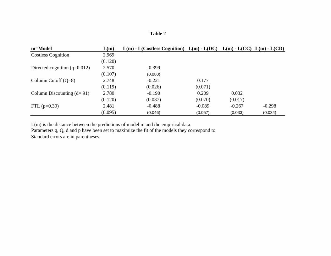
m=Model L(m) L(m) - L(Costless Cognition) L(m) - L(DC) L(m) - L(CC) L(m) - L(CD)Costless Cognition 2.969

(0.120)Directed cognition (q=0.012) 2.570 -0.399

(0.107) (0.080)Column Cutoff (Q=8) 2.748 -0.221 0.177

(0.119) (0.026) (0.071)Column Discounting (d=.91) 2.780 -0.190 0.209 0.032

(0.120) (0.037) (0.070) (0.017)FTL (p=0.30) 2.481 -0.488 -0.089 -0.267 -0.298

(0.095) (0.046) (0.057) (0.033) (0.034)

L(m) is the distance between the predictions of model m and the empirical data. Parameters q, Q, d and p have been set to maximize the fit of the models they correspond to.

Table 2

Standard errors are in parentheses.