Bounded inhomogeneous wave profiles for increased surfacewave excitation efficiency at fluid–solid interfaces

Daniel C. Woods, J. Stuart Bolton, and Jeffrey F. Rhoadsa)

School of Mechanical Engineering, Ray W. Herrick Laboratories, and Birck Nanotechnology Center,Purdue University, West Lafayette, Indiana 47907, USA

(Received 13 June 2016; revised 5 March 2017; accepted 20 March 2017; published online 20April 2017)

Though the ultrasonic excitation of surface waves in solids is generally realized through the use of

a contact transducer, remote excitation would enable standoff testing in applications such as the

nondestructive evaluation of structures. With respect to the optimal incident wave profile, bounded

inhomogeneous waves, which include an exponentially decaying term, have been shown to improve

the surface wave excitation efficiency as compared to Gaussian and square waves. The purpose of

this work is to investigate the effect of varying the incident wave spatial decay rate, as applied to

both lossless fluid–solid interfaces and to solids with viscoelastic losses included. The Fourier

method is used to decompose the incident profile and subsequently compute the reflected wave pro-

file. It is shown that inhomogeneous plane wave theory predicts, to a close approximation, the loca-

tion of the minimum in the local reflection coefficient with respect to the decay rate for bounded

incident waves. Moreover, plane wave theory gives a reasonable indication of the decay rate that

maximizes the surface wave excitation efficiency. VC 2017 Acoustical Society of America.

[http://dx.doi.org/10.1121/1.4979595]

[KML] Pages: 2779–2787

I. INTRODUCTION

The excitation of surface waves on solid media is of

interest in a number of contexts, including nondestructive

testing1,2 and seismology.3 Though in typical applications

body and surface waves are excited in the solid by means of

a contact transducer, remote, non-contact excitation would

enable testing from a standoff distance, which may prove

useful, for instance, in the nondestructive evaluation of

structures,4–6 in medical ultrasound imaging,7,8 and in other

applications where the use of a couplant is undesirable.9–11

The excitation of Rayleigh-type surface waves by incident

acoustic plane waves has previously been considered in

depth,12–14 as has the excitation by bounded incident waves

having a Gaussian profile.15–18 More recently, excitation by

other types of bounded ultrasonic beams has been investi-

gated experimentally and has been confirmed to produce

both specular and nonspecular reflected portions, corre-

sponding to subsurface transmission and the excitation of

solid surface waves.19–21 However, little attention has been

given to the effect of tuning the waveform to enhance the

surface wave excitation efficiency.

To this end, Vanaverbeke et al.22 considered more gen-

eral incident wave profiles, termed “bounded inhomoge-

neous waves,” where a component of exponential decay was

introduced perpendicular to the propagation direction. Their

work drew a strong connection between the reflection and

transmission of the bounded incident waves at the fluid–

solid interface and inhomogeneous plane wave theory,

where the local reflection coefficient in the specular direc-

tion was observed to remain close to that predicted by plane

wave theory, particularly for larger beamwidths. More

importantly, it was shown that the surface wave excitation

efficiency for the bounded inhomogeneous incident waves

was substantially higher than that for Gaussian and square

profiles. Interestingly, previous work has shown that, by tun-

ing the decay rate of incident inhomogeneous plane waves,

a zero of the reflection coefficient can be achieved near the

Rayleigh angle for lossless fluid–solid interfaces,23 and

near-zero values can be achieved for low-loss, viscoelastic

fluid–solid interfaces.24 Though Vanaverbeke et al.,22 along

with others,13,21,25,26 have given a detailed account of the

effects of the frequency, beamwidth, and steepness of the

incident profiles, they have not reported tuning the decay

parameter to improve the surface wave excitation efficiency.

It is thus the purpose of the present work to demonstrate

that inhomogeneous plane wave theory can be used to

approximate the optimal spatial decay rate of bounded inci-

dent waves that maximizes the surface wave excitation effi-

ciency near the Rayleigh angle. Moreover, these predictions

for lossless solid interfaces will be extended to low-loss vis-

coelastic solid interfaces by using the theory for linear vis-

coelastic media. In this effort, the form of the wave profile

at the interface surface will be varied, in terms of the speci-

fied rate of spatial exponential decay and effective beam-

width, to investigate the effect on the surface wave

generation.

With regard to the specification of the incident wave pro-

file, in practice, the form may be prescribed at some standoff

distance from the interface, in which case the propagation

effect of the bounded wave over the nonzero offset distance

would necessarily cause distortion of the profile at the inter-

face surface. This effect on both the profile amplitude and

phase, which may be of significant interest in a number ofa)Electronic mail: jfrhoads@purdue.edu

J. Acoust. Soc. Am. 141 (4), April 2017 VC 2017 Acoustical Society of America 27790001-4966/2017/141(4)/2779/9/$30.00

practical systems, is discussed in the Appendix. However, the

aim of this work is to isolate the effect of the waveform

parameters at the interface on the excitation efficiency, so the

profile will be prescribed explicitly along the interface sur-

face. Though considerations for a practical implementation of

this condition lie beyond the scope of the present work, it

should be noted here that, in a real system, this condition

would need to be carefully controlled by appropriate sound

field reproduction techniques,27–29 in conjunction with fluid–

coupled transducers, to ensure that the amplitude and phase

information generated along the interface match (within an

appropriate tolerance) that which is prescribed.

The well-known Fourier method12,15–18,22 will be uti-

lized in this work to compute the reflected wave profiles,

from which the energy fluxes and surface wave excitation

efficiency can be subsequently calculated. In addition to the

excitation efficiency, the correspondence between the local

reflection coefficient (taken at a specific point along the

interface) as a function of the incident wave decay rate and

that predicted by plane wave theory will also be presented.

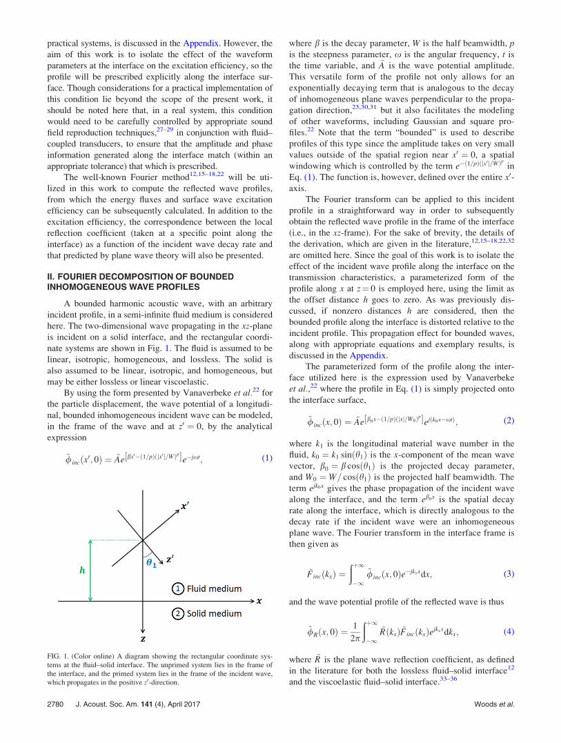
II. FOURIER DECOMPOSITION OF BOUNDEDINHOMOGENEOUS WAVE PROFILES

A bounded harmonic acoustic wave, with an arbitrary

incident profile, in a semi-infinite fluid medium is considered

here. The two-dimensional wave propagating in the xz-plane

is incident on a solid interface, and the rectangular coordi-

nate systems are shown in Fig. 1. The fluid is assumed to be

linear, isotropic, homogeneous, and lossless. The solid is

also assumed to be linear, isotropic, and homogeneous, but

may be either lossless or linear viscoelastic.

By using the form presented by Vanaverbeke et al.22 for

the particle displacement, the wave potential of a longitudi-

nal, bounded inhomogeneous incident wave can be modeled,

in the frame of the wave and at z0 ¼ 0, by the analytical

expression

~/incðx0; 0Þ ¼ ~Ae bx0�ð1=pÞðjx0 j=WÞp½ �e�jxt; (1)

where b is the decay parameter, W is the half beamwidth, pis the steepness parameter, x is the angular frequency, t is

the time variable, and ~A is the wave potential amplitude.

This versatile form of the profile not only allows for an

exponentially decaying term that is analogous to the decay

of inhomogeneous plane waves perpendicular to the propa-

gation direction,23,30,31 but it also facilitates the modeling

of other waveforms, including Gaussian and square pro-

files.22 Note that the term “bounded” is used to describe

profiles of this type since the amplitude takes on very small

values outside of the spatial region near x0 ¼ 0, a spatial

windowing which is controlled by the term e�ð1=pÞðjx0j=WÞp in

Eq. (1). The function is, however, defined over the entire x0-axis.

The Fourier transform can be applied to this incident

profile in a straightforward way in order to subsequently

obtain the reflected wave profile in the frame of the interface

(i.e., in the xz-frame). For the sake of brevity, the details of

the derivation, which are given in the literature,12,15–18,22,32

are omitted here. Since the goal of this work is to isolate the

effect of the incident wave profile along the interface on the

transmission characteristics, a parameterized form of the

profile along x at z¼ 0 is employed here, using the limit as

the offset distance h goes to zero. As was previously dis-

cussed, if nonzero distances h are considered, then the

bounded profile along the interface is distorted relative to the

incident profile. This propagation effect for bounded waves,

along with appropriate equations and exemplary results, is

discussed in the Appendix.

The parameterized form of the profile along the inter-

face utilized here is the expression used by Vanaverbeke

et al.,22 where the profile in Eq. (1) is simply projected onto

the interface surface,

~/incðx; 0Þ ¼ ~Ae b0x�ð1=pÞðjxj=W0Þp½ �ejðk0x�xtÞ; (2)

where k1 is the longitudinal material wave number in the

fluid, k0 ¼ k1 sinðh1Þ is the x-component of the mean wave

vector, b0 ¼ b cosðh1Þ is the projected decay parameter,

and W0 ¼ W= cosðh1Þ is the projected half beamwidth. The

term ejk0x gives the phase propagation of the incident wave

along the interface, and the term eb0x is the spatial decay

rate along the interface, which is directly analogous to the

decay rate if the incident wave were an inhomogeneous

plane wave. The Fourier transform in the interface frame is

then given as

~FincðkxÞ ¼ðþ1�1

~/incðx; 0Þe�jkxxdx; (3)

and the wave potential profile of the reflected wave is thus

~/R x; 0ð Þ ¼ 1

2p

ðþ1�1

~R kxð Þ ~Finc kxð Þejkxxdkx; (4)

where ~R is the plane wave reflection coefficient, as defined

in the literature for both the lossless fluid–solid interface12

and the viscoelastic fluid–solid interface.33–36

FIG. 1. (Color online) A diagram showing the rectangular coordinate sys-

tems at the fluid–solid interface. The unprimed system lies in the frame of

the interface, and the primed system lies in the frame of the incident wave,

which propagates in the positive z0-direction.

2780 J. Acoust. Soc. Am. 141 (4), April 2017 Woods et al.

III. EFFICIENCY OF RAYLEIGH-TYPE SURFACE WAVEEXCITATION

When a bounded acoustic beam is incident on a solid

surface near the Rayleigh angle, a portion of the incident

energy is transmitted into the solid and carried within the

solid medium along the interface (i.e., in the x-direction in

Fig. 1).15,22,32 This energy flux generates a Rayleigh-type

surface wave in the solid, which then reradiates energy into

the fluid to form the displaced portion of the reflected profile.

This shift of the reflected wave along the interface has been

described in detail for Gaussian incident profiles15,32 and for

bounded inhomogeneous incident profiles.13,20,22 There thus

exists, near the incident beam, a power flux at any given

position x along the interface which will be reradiated into

the fluid by the excitation of the surface wave.

In order to quantify the surface wave generation by

bounded inhomogeneous incident waves, the surface wave

excitation efficiency, as a function of the position along the

interface, can be defined as the difference between the inci-

dent and reflected intensities normal to the interface, inte-

grated from �1 to x and normalized with respect to the

total incident normal intensity22,32

g xð Þ ¼

ðx

�1jIinc;z n; 0ð Þj � jIR;z n; 0ð Þj� �

dnðþ1�1jIinc;z n; 0ð Þjdn

; (5)

where Iinc;z and IR;z are the normal intensities of the incident

and reflected waves, respectively. The intensities for each

wave, denoted with the subscript m, are straightforward to

compute in the lossless fluid as Im;z ¼ Re½�~rm;zz~v�m;z�=2,

where Re denotes the real part of the argument, � denotes

the complex conjugate, ~rm;zz ¼ �q1x2 ~/m is the associated

normal stress (q1 is the density of the fluid), and ~vm;z is the

associated normal velocity

~vinc;z x; 0ð Þ ¼ x2p

ðþ1�1

~kz~Finc kxð Þejkxxdkx;

~vR;z x; 0ð Þ ¼ x2p

ðþ1�1�~kz

~R kxð Þ ~Finc kxð Þejkxxdkx; (6)

where ~kz ¼ffiffiffiffiffiffiffiffiffiffiffiffiffiffiffik2

1 � k2x

pis evaluated as the principal square

root36 and is the z-component of the constituent wave vector.

The surface wave excitation efficiency takes on its maximum

value at a position xmax, beyond which point the reflected

normal intensity exceeds the incident intensity. However, it

should be noted that, for the case of a plane incident wave,

the excitation efficiency is independent of the position along

the interface, since the ratio of the incident and reflected

wave amplitudes is a function only of the plane wave reflec-

tion coefficient. Equation (5) thus simplifies, for a plane

wave, to g ¼ 1� j ~Rj2.

It should be further emphasized here that the surface

wave excitation efficiency in Eq. (5) and the incident and

reflected profiles in Eqs. (2) and (4) specify the energy flux

and pressure field at the interface (i.e., at any x-value along

z¼ 0). Since this work is focused on finding the incident

wave parameters which yield minimal reflection and maxi-

mal excitation efficiency at the interface, these quantities at

z¼ 0 are sufficient. Note, however, that away from the inter-

face, the reflected profile lies along a plane perpendicular to

its associated mean wave vector, which is in general not

aligned with the interface for oblique incidence.13,19,22

IV. NUMERICAL RESULTS AND DISCUSSION

In order to illustrate the effect of the spatial decay rate of

the incident wave on the surface wave generation at fluid–

solid interfaces, a water–stainless steel interface is considered

here. The frequency was set to f¼ 4 MHz (f ¼ x=½2p�),which is within the range for typical ultrasonic nondestructive

testing applications. The densities and wave speeds of the two

media were taken to be those used by Vanaverbeke et al.:22

for water, density q1 ¼ 1000 kg/m3 and longitudinal

wave speed c1 ¼ 1480 m/s; and for stainless steel, density

q2 ¼ 7900 kg/m3, longitudinal wave speed c2 ¼ 5790 m/s,

and shear wave speed b2 ¼ 3100 m/s. For the case in which

viscoelastic losses in the stainless steel are included, which is

considered in Sec. IV B, the longitudinal and shear wave

attenuation coefficients at the given frequency were taken,

respectively, to be ac2¼ 16:0 rad/m and ab2

¼ 50:8 rad/m,

which were computed from the inverse quality factors used

by Borcherdt36 for stainless steel. The steepness parameter in

Eq. (1) was set to p¼ 8 for the bounded inhomogeneous inci-

dent profiles,22 and the wave potential amplitude ~A was taken

to be an arbitrary constant.

To illustrate the form of the incident and reflected wave

profiles, several incident profiles are presented in Fig. 2(a),

and an incident profile along with the corresponding

reflected profile at the lossless water–stainless steel interface

are shown in Fig. 2(b), with incidence at h1 ¼ 30:968�, near

the Rayleigh angle. The shift of the peak in the reflected

wave profile along the interface is analogous to the shift

observed for Gaussian incident waves.15,32 For a detailed

account of the form of the incident and reflected profiles, the

reader is referred to the work of Vanaverbeke et al.22

In addition to the surface wave excitation efficiency

defined by Eq. (5), the local reflection coefficient,22 defined

as the ratio j~/Rj=j~/incj, was considered at x ¼ z ¼ 0 as a

measure of the local transmission efficiency at this point.

Specifically, the effect of the decay parameter b was of inter-

est here.

A. Water–stainless steel interface

For the lossless water–stainless steel interface, the mag-

nitude of the reflection coefficient for an incident inhomoge-

neous plane wave and the magnitude of the local reflection

coefficient for several bounded inhomogeneous incident

waves are presented in Fig. 3 as a function of the decay

parameter b. The waves are incident at the angle that mini-

mizes the reflection coefficient, h1 ¼ 30:968�, which is near

the Rayleigh angle. For the plane wave, the decay parameter

gives the rate of exponential decay perpendicular to the

propagation direction.23,30,31 As is evident, the form of the

plane wave reflection coefficient, including the location of

the minimum, is closely matched by the local reflection

J. Acoust. Soc. Am. 141 (4), April 2017 Woods et al. 2781

coefficients for the wider beamwidths. The decay parameter

which yields the minimum for the profile with the half beam-

width W¼ 30 mm is b ¼ 110:8 rad/m, which gives a 0:18%

error with respect to the value for the plane incident wave,

b ¼ 111:0 rad/m. Moreover, as expected, the correspon-

dence between this decay value for bounded waves and that

predicted by plane wave theory is found to be exact in the

limit of large beamwidths. The profile with the smallest

beamwidth in Fig. 3, however, shows a considerable shift to

a lower value of the decay parameter required to yield the

minimum. This is due to the fact that narrower beamwidths

inherently possess a greater degree of inhomogeneity (as the

spatial windowing dominates over a larger portion of the

profile), and so less inhomogeneity must be introduced

through the exponentially decaying term in order to achieve

the optimal level of inhomogeneity. Also of note in Fig. 3(b)

is the small nonzero value of the reflection coefficient at the

minimum for the bounded wave profiles, as opposed to the

zero value for the incident plane wave. The nonzero mini-

mum value is attributable to the effect of the presence of the

suboptimal wave vector components which are inherent in

the bounded wave profile and which are quantified by the

decomposition in Eq. (3).

Figure 4 shows the surface wave excitation efficiency,

evaluated at the critical point xmax that yields the maximum

efficiency, as a function of the decay parameter and half

beamwidth of the incident wave. The global maximum of

the excitation efficiency is observed at a decay parameter of

b ¼ 134:2 rad/m and a half beamwidth of W¼ 7.7 mm, which

yield an efficiency of gðxmaxÞ ¼ 92:8%. Vanaverbeke et al.22

noted the local maximum with respect to the beamwidth, and

the results presented here indicate that a maximum with

FIG. 2. (Color online) (a) Several incident bounded wave profiles (p¼ 8) of half beamwidth W¼ 20 mm, with decay parameters b¼ 50 rad/m (� markers),

b¼ 100 rad/m (triangular markers), and b¼ 200 rad/m (square markers); and (b) an incident bounded wave profile (W¼ 20 mm, b¼ 50 rad/m, p¼ 8;

� markers) along with the reflected wave profile (triangular markers) for the water–stainless steel interface at 4 MHz, with losses neglected.

FIG. 3. (Color online) The magnitude of the reflection coefficient for the water–stainless steel interface at 4 MHz, with losses neglected, as a function of the

incident wave decay parameter b. The incident waves are specified as an inhomogeneous plane wave (unmarked curve), and bounded wave profiles (p¼ 8) of

half beamwidths W¼ 10 mm (� markers), W¼ 20 mm (triangular markers), and W¼ 30 mm (square markers). The curves for the inhomogeneous plane wave

and bounded wave profile of half beamwidth W¼ 30 mm are nearly coincident. Note that (b) gives a zoomed-in view near the local minima.

2782 J. Acoust. Soc. Am. 141 (4), April 2017 Woods et al.

respect to the decay parameter can also be located. As a

point of comparison with more common incident wave pro-

files, the peaks in the excitation efficiency with respect to the

beamwidth for Gaussian (b¼ 0, p¼ 2) and square (b¼ 0,

p¼ 8) waves are found to be 80.2% and 80.9%, respectively.

The use of the bounded inhomogeneous profiles considered

here, with the optimal decay parameter and beamwidth, thus

yields an improvement of approximately 12%–13% over

those more common profiles. This improvement is even

more pronounced for beamwidths which are larger than that

at the peak value, and the relative increase in the excitation

efficiency at a half beamwidth of 50 mm, for example,

exceeds 50% as compared to both Gaussian and square inci-

dent waves (see also Ref. 22). As is evident in Fig. 4, the

value of the decay parameter which yields the global maxi-

mum lies above the value which yields the reflection coeffi-

cient minimum, and this result is attributable to the greater

spatial concentration of the incident wave’s energy for the

higher spatial decay rates. As such, the peak in the fraction

of the power flux available for surface wave generation is

larger for greater decay rates, and the energy is reradiated

over a larger distance (i.e., the peak in the reflected wave

profile is shifted farther along the interface). Moreover, for

beamwidths larger than the width which yields the global

maximum, the optimal decay parameter is shifted to higher

values since the greater spatial concentration of the incident

wave provided by larger decay values is more significant for

the larger beamwidths. This effect is balanced by the

increased transmission at the local minimum of the reflection

coefficient at lower decay parameter values.

Figure 5 presents the surface wave excitation efficiency

as a function of the decay parameter at the same half beam-

widths as were used for calculating the reflection coefficients

shown in Fig. 3, along with that for a plane incident wave,

where the decay parameter range is increased to show the

maximum for each beamwidth. For the plane wave, the peak

in the excitation efficiency (which reaches an efficiency of

100%) is observed to occur at the exact decay value which

yields the zero of the reflection coefficient, and the shift in

the optimal decay rate to higher values for the bounded

waves, which increases with beamwidth, is readily apparent.

It should also be noted that, for the case of a homogeneous

plane incident wave (i.e., b¼ 0), though stress fields are

induced near the solid surface, at any given point along the

interface, the energy from the incident wave is entirely

reflected back into the fluid, and thus no energy is available

for surface wave excitation at other points on the interface,

which is shown by the zero value of the efficiency in Fig. 5.

B. Effect of viscoelastic losses in the solid medium

The effect of viscoelastic losses in the solid medium is

considered here for the water–stainless steel interface. The

magnitude of the reflection coefficient for an incident inho-

mogeneous plane wave and for several bounded inhomoge-

neous incident waves (using the local reflection coefficient)

is presented in Fig. 6, with the waves again incident near the

Rayleigh angle to minimize the reflection coefficient. It

should be noted that this optimal angle, h1 ¼ 30:973�, is

slightly shifted relative to the lossless case. As is evident in

Fig. 6, the main effect of the incorporation of the viscoelastic

losses is the shift in the minimum of the reflection coefficient

to significantly smaller values of the decay parameter. Since

losses in the solid medium introduce additional levels of

inhomogeneity in the transmitted waves, a smaller degree of

inhomogeneity is necessary to optimize the transmission, as

was previously noted for the case of incident inhomogeneous

plane waves.24 Moreover, the plane wave reflection coeffi-

cient magnitude remains less than unity even when the inci-

dent wave is homogeneous (b¼ 0), due to the losses in the

solid. As can be observed, the reflection coefficients for the

bounded wave profiles again closely match that of the plane

wave for the larger beamwidths. Also of note is the increase

FIG. 4. (Color online) The surface wave excitation efficiency, evaluated at

the critical point xmax, for the water–stainless steel interface at 4 MHz, with

losses neglected, as a function of the incident wave decay parameter b and

half beamwidth W for the bounded incident wave profiles (p¼ 8). The

þ marker indicates the global maximum.

FIG. 5. (Color online) The surface wave excitation efficiency, evaluated at

the critical point xmax, for the water–stainless steel interface at 4 MHz, with

losses neglected, as a function of the incident wave decay parameter b. The

incident waves are specified as an inhomogeneous plane wave (unmarked

curve), and bounded wave profiles (p¼ 8) of half beamwidths W¼ 10 mm

(� markers), W¼ 20 mm (triangular markers), and W¼ 30 mm (square

markers). The solid, circular markers indicate the maxima for the respective

incident waves.

J. Acoust. Soc. Am. 141 (4), April 2017 Woods et al. 2783

in the reflection coefficient value at the minimum as com-

pared to the lossless case, which is particularly evident for

the narrowest beamwidth, W¼ 10 mm, in Fig. 6(b). This

result also follows from the introduction of material damp-

ing, which increases the value at the local minimum.

Figure 7 shows the surface wave excitation efficiency,

again evaluated at the critical point xmax, as a function of the

decay parameter and half beamwidth with the viscoelastic

losses in stainless steel included. A global maximum can

again be found but, with respect to the lossless case, the cor-

responding decay parameter is shifted to a lower value and

the corresponding beamwidth is shifted to a higher value.

This optimal decay rate, however, is still above the decay

rate which yields the minimum of the reflection coefficient

for the viscoelastic case. Interestingly, for beamwidths larger

than that which yields the global maximum of the excitation

efficiency, the optimal decay parameter decreases with

increasing beamwidth, and this decay value ultimately falls

below that which gives the reflection coefficient minimum.

This effect may be due to the greater levels of inhomogene-

ity introduced in the transmitted waves by the material

damping for the larger beamwidths, since these wave profiles

experience the effects of the viscoelastic losses over a

greater distance along the interface.

Finally, Fig. 8 gives the surface wave excitation effi-

ciency as a function of just the decay parameter for the same

half beamwidths as were previously considered, along with

that for a plane incident wave. As for the lossless case, the

FIG. 6. (Color online) The magnitude of the reflection coefficient for the water–stainless steel interface at 4 MHz, with the viscoelastic losses in steel included,

as a function of the incident wave decay parameter b. The incident waves are specified as an inhomogeneous plane wave (unmarked curve), and bounded

wave profiles (p¼ 8) of half beamwidths W¼ 10 mm (� markers), W¼ 20 mm (triangular markers), and W¼ 30 mm (square markers). The curves for the inho-

mogeneous plane wave and bounded wave profile of half beamwidth W¼ 30 mm are nearly coincident. Note that (b) gives a zoomed-in view near the local

minima.

FIG. 7. (Color online) The surface wave excitation efficiency, evaluated at

the critical point xmax, for the water–stainless steel interface at 4 MHz, with

the viscoelastic losses in steel included, as a function of the incident wave

decay parameter b and half beamwidth W for the bounded incident wave

profiles (p¼ 8). The þ marker indicates the global maximum.

FIG. 8. (Color online) The surface wave excitation efficiency, evaluated at

the critical point xmax, for the water–stainless steel interface at 4 MHz, with

the viscoelastic losses in steel included, as a function of the incident wave

decay parameter b. The incident waves are specified as an inhomogeneous

plane wave (unmarked curve), and bounded wave profiles (p¼ 8) of half

beamwidths W¼ 10 mm (� markers), W¼ 20 mm (triangular markers), and

W¼ 30 mm (square markers). The solid, circular markers indicate the max-

ima for the respective incident waves.

2784 J. Acoust. Soc. Am. 141 (4), April 2017 Woods et al.

excitation efficiency for the plane incident wave reaches its

maximum at the value of the decay parameter which yields

the minimum of the reflection coefficient. Since the half

beamwidth W¼ 10 mm lies below that which gives the

global maximum for this case, the decay parameter which

yields the peak efficiency is shifted to larger values, whereas

the other two beamwidths shown in Fig. 8 lie above the

global maximum and therefore show shifts to smaller decay

parameter values to yield the respective peaks in excitation

efficiency. Also note that the value of the efficiency for the

homogeneous plane wave case (b¼ 0) is nonzero due to

the losses in the solid. It follows that the excitation effi-

ciency for the bounded wave profiles increases with

increasing beamwidth in the limit of small values of the

decay parameter.

V. CONCLUSIONS

A comparison of the predictions for the reflection coeffi-

cient and for the surface wave excitation efficiency of inci-

dent plane waves and incident bounded inhomogeneous

waves as a function of the incident wave spatial decay rate

has been presented for a lossless fluid–solid interface and

also with viscoelastic losses included in the solid. This work

extends that of Vanaverbeke et al.,22 who demonstrated that

bounded inhomogeneous waves improve the surface wave

excitation efficiency as compared to Gaussian and square

waves, by examining the effect of tuning the decay parame-

ter. It was shown here that the minimum in the plane wave

reflection coefficient with respect to the decay parameter23,24

provides a good prediction of the minimum in the local

reflection coefficient for bounded wave profiles, which is

exact in the limit of large beamwidths. Inhomogeneous plane

wave theory also provides an indication of the decay param-

eter value which maximizes the surface wave excitation effi-

ciency, but this value is sensitive to the beamwidth of

bounded waves and there is generally a shift to larger decay

parameter values due to the greater spatial concentration of

the incident wave energy at those larger decay rates. The

incorporation of viscoelastic losses in the solid, however,

has the effect of introducing additional inhomogeneity to the

transmitted waves, and so lower values of the decay parame-

ter were found to yield the maximum excitation efficiency

with the losses included.

The results presented here, which demonstrate that an

optimal value of the incident wave decay rate can be identi-

fied with incidence near the Rayleigh angle, may prove use-

ful for non-contact excitation in applications such as

nondestructive testing1,2,4–6 and medical ultrasound imag-

ing.7,8 Moreover, these waveforms may be generated in prac-

tice by sound field reproduction techniques with phased

arrays of sources,29,37–39 or by other approaches,27,28,31,40

though the distortion of the profile over nonzero standoff dis-

tances would have to be carefully controlled in such an

implementation (see also the Appendix). The generation of

bounded inhomogeneous waves of the type considered in

this work, in particular, was investigated by Declercq and

Leroy,26 and it was noted that a reasonable approximation

may be achievable in the near field.

In future work, sound field reproduction techniques for

these types of bounded inhomogeneous wave profiles will be

investigated, specifically through the use of source arrays. In

addition, experimental validation of the theoretical predic-

tions of the optimal surface wave excitation efficiency will

be pursued. This work will continue the investigation of

methods for increased acoustic transmission across fluid–

solid interfaces through analysis and experimentation.

ACKNOWLEDGMENTS

This research is funded by the U.S. Office of Naval

Research through ONR Grant Nos. N00014-10-1-0958 and

N00014-16-1-2275.

APPENDIX: PROPAGATION EFFECT FOR BOUNDEDINHOMOGENEOUS WAVES

With reference to Fig. 1, if the incident wave profile

given by Eq. (1) is prescribed in the frame of the wave at

z0 ¼ 0, then the Fourier decomposition into the plane wave

spectrum must also be implemented at z0 ¼ 0. The associated

Fourier transform is then15,32

~Fincðkx0 Þ ¼ðþ1�1

~/incðx0; 0Þe�jkx0 x0dx0: (A1)

The coordinate transformation to the interface frame is

given by

x0 ¼ x cosðh1Þ � ðhþ zÞ sinðh1Þ;z0 ¼ x sinðh1Þ þ ðhþ zÞ cosðh1Þ: (A2)

Therefore, by using the coordinates and wave vector compo-

nents in the interface frame, the incident wave profile can be

written at an arbitrary position (where z< 0) as

~/inc x; zð Þ ¼1

2p

ðþ1�1

~Finc kxð Þejkxxþjkz zþhð Þdkx: (A3)

To compute the reflected profile is also straightforward

~/R x; zð Þ ¼1

2p

ðþ1�1

~R kxð Þ ~Finc kxð Þejkxx�jkz z�hð Þdkx: (A4)

This approach to the computation of the profile at the

interface (i.e., evaluating the expressions at z¼ 0) fully

accounts for the propagation effect and resulting distortion

of the bounded profile at the interface for arbitrary offset dis-

tances h. In the present work, the profile was instead pre-

scribed along the interface itself, in order to isolate the effect

of the wave profile alone. However, for the purpose of pro-

viding a brief discussion of this propagation effect, which is

of interest in practical implementations, results for the dis-

tortion effect for several exemplary cases are presented here.

The water–stainless steel interface at 4 MHz considered in

Sec. IV A is again considered here, with the incidence angle

set at h1 ¼ 30:968�, near the Rayleigh angle. Figure 9 shows

the amplitude distortion at the interface (z¼ 0) for an exem-

plary bounded wave profile of half beamwidth W¼ 20 mm

J. Acoust. Soc. Am. 141 (4), April 2017 Woods et al. 2785

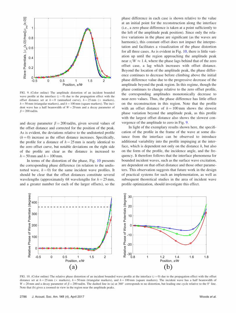
and decay parameter b¼ 200 rad/m, given several values of

the offset distance and corrected for the position of the peak.

As is evident, the deviations relative to the undistorted profile

(h¼ 0) increase as the offset distance increases. Specifically,

the profile for a distance of h¼ 25 mm is nearly identical to

the zero offset curve, but notable deviations on the right side

of the profile are clear as the distance is increased to

h¼ 50 mm and h¼ 100 mm.

In terms of the distortion of the phase, Fig. 10 presents

the corresponding phase difference (in relation to the undis-

torted wave, h¼ 0) for the same incident wave profiles. It

should be clear that the offset distances constitute several

wavelengths (approximately 68 wavelengths for h¼ 25 mm,

and a greater number for each of the larger offsets), so the

phase difference in each case is shown relative to the value

at an initial point for the reconstruction along the interface

(i.e., a zero phase difference is taken at a point sufficiently to

the left of the amplitude peak position). Since only the rela-

tive variations in the phase are significant (as the waves are

harmonic), this constant offset does not impact the interpre-

tation and facilitates a visualization of the phase distortion

for all three cases. As is evident in Fig. 10, there is little vari-

ation up until the region approaching the amplitude peak

near x=W � 1:4, where the phase lags behind that of the zero

offset case, a lag which increases with offset distance.

Beyond the location of the amplitude peak, the phase differ-

ence continues to decrease before climbing above the initial

phase difference value due to the progressive decrease of the

amplitude beyond the peak region. In this regime, though the

phase continues to change relative to the zero offset profile,

the corresponding amplitudes monotonically decrease to

near-zero values. Thus, the phase difference has little effect

on the reconstruction in this region. Note that the profile

with an offset distance of h¼ 100 mm shows the slowest

phase variation beyond the amplitude peak, as this profile

with the largest offset distance also shows the slowest con-

vergence of the amplitude to zero in Fig. 9.

In light of the exemplary results shown here, the specifi-

cation of the profile in the frame of the wave at some dis-

tance from the interface can be observed to introduce

additional variability into the profile impinging at the inter-

face, which is dependent not only on the distance h, but also

on the form of the profile, the incidence angle, and the fre-

quency. It therefore follows that the interface phenomena for

bounded incident waves, such as the surface wave excitation,

are dependent on that offset distance and those other parame-

ters. This observation suggests that future work in the design

of practical systems for such an implementation, as well as

subsequent theoretical studies in the area of incident wave

profile optimization, should investigate this effect.

FIG. 9. (Color online) The amplitude distortion of an incident bounded

wave profile at the interface (z¼ 0) due to the propagation effect with the

offset distance set at h¼ 0 (unmarked curve), h¼ 25 mm (� markers),

h¼ 50 mm (triangular markers), and h¼ 100 mm (square markers). The inci-

dent wave has a half beamwidth of W¼ 20 mm and a decay parameter of

b¼ 200 rad/m.

FIG. 10. (Color online) The relative phase distortion of an incident bounded wave profile at the interface (z¼ 0) due to the propagation effect with the offset

distance set at h¼ 25 mm (� markers), h¼ 50 mm (triangular markers), and h¼ 100 mm (square markers). The incident wave has a half beamwidth of

W¼ 20 mm and a decay parameter of b¼ 200 rad/m. The dashed line in (a) at 360� corresponds to no distortion, but leading one cycle relative to the 0� line.

Note that (b) gives a zoomed-in view in the region near the amplitude peaks.

2786 J. Acoust. Soc. Am. 141 (4), April 2017 Woods et al.

1F. R. Rollins, Jr., “Critical ultrasonic reflectivity: A neglected tool for

material evaluation,” Mater. Eval. 24(12), 683–689 (1966).2C. E. Fitch, Jr. and R. L. Richardson, “Ultrasonic wave models for nonde-

structive testing interfaces with attenuation,” in Progress in AppliedMaterials Research, edited by E. G. Stanford, J. H. Fearon, and W. J.

McGounagle (Iliffe Books, London, England, 1967), Vol. 8, pp. 79–120.3K. Aki and P. G. Richards, Quantitative Seismology: Theory and Methods(W. H. Freeman and Company, San Francisco, CA, 1980), Vol. 1, 557 pp.

4J. Yang, N. DeRidder, C. Ume, and J. Jarzynski, “Non-contact optical fibre

phased array generation of ultrasound for non-destructive evaluation of

materials and processes,” Ultrasonics 31(6), 387–394 (1993).5J. Peters, V. Kommareddy, Z. Liu, D. Fei, and D. Hsu, “Non-contact

inspection of composites using air-coupled ultrasound,” AIP Conf. Proc.

657(22), 973–980 (2003).6R. E. Green, “Non-contact ultrasonic techniques,” Ultrasonics 42(1), 9–16

(2004).7L. Gao, K. J. Parker, R. M. Lerner, and S. F. Levinson, “Imaging of the

elastic properties of tissue: A review,” Ultrasound Med. Biol. 22(8),

959–977 (1996).8G. Rousseau, B. Gauthier, A. Blouin, and J. P. Monchalin, “Non-contact

biomedical photoacoustic and ultrasound imaging,” J. Biomed. Opt. 17(6),

061217 (2012).9M. C. Bhardwaj, “Innovation in non-contact ultrasonic analysis:

Applications for hidden objects detection,” Mater. Res. Innov. 1(3),

188–196 (1997).10T. H. Gan, P. Pallav, and D. A. Hutchins, “Non-contact ultrasonic quality

measurements of food products,” J. Food Eng. 77(2), 239–247 (2006).11S. Meyer, S. A. Hindle, J. P. Sandoz, T. H. Gan, and D. A. Hutchins,

“Non-contact evaluation of milk-based products using air-coupled ultra-

sound,” Measurement Sci. Technol. 17(7), 1838–1846 (2006).12L. M. Brekhovskikh, Waves in Layered Media (Academic Press, New

York, 1960), 561 p.13N. F. Declercq, R. Briers, J. Degrieck, and O. Leroy, “The history and

properties of ultrasonic inhomogeneous waves,” IEEE Trans. Ultrason.

Ferroelectr. Frequency Control 52(5), 776–791 (2005).14J. D. N. Cheeke, Fundamentals and Applications of Ultrasonic Waves

(CRC Press, Boca Raton, FL, 2012), pp. 125–134.15H. L. Bertoni and T. Tamir, “Unified theory of Rayleigh-angle phenomena

for acoustic beams at liquid-solid interfaces,” Appl. Phys. 2(4), 157–172

(1973).16M. A. Breazeale, L. Adler, and L. Flax, “Reflection of a Gaussian ultra-

sonic beam from a liquid–solid interface,” J. Acoust. Soc. Am. 56(3),

866–872 (1974).17M. A. Breazeale, L. Adler, and G. W. Scott, “Interaction of ultrasonic

waves incident at the Rayleigh angle onto a liquid–solid interface,”

J. Appl. Phys. 48(2), 530–537 (1977).18T. D. Ngoc and W. G. Mayer, “Numerical integration method for reflected

beam profiles near Rayleigh angle,” J. Acoust. Soc. Am. 67(4),

1149–1152 (1980).19Y. Bouzidi and D. R. Schmitt, “Acoustic reflectivity goniometry of

bounded ultrasonic pulses: Experimental verification of numerical mod-

els,” J. Appl. Phys. 104(6), 064914 (2008).20N. F. Declercq and E. Lamkanfi, “Study by means of liquid side acoustic

barrier of the influence of leaky Rayleigh waves on bounded beam

reflection,” Appl. Phys. Lett. 93(5), 054103 (2008).

21N. F. Declercq, “Experimental study of ultrasonic beam sectors for energy

conversion into Lamb waves and Rayleigh waves,” Ultrasonics 54(2),

609–613 (2014).22S. Vanaverbeke, F. Windels, and O. Leroy, “The reflection of bounded

inhomogeneous waves on a liquid/solid interface,” J. Acoust. Soc. Am.

113(1), 73–83 (2003).23D. C. Woods, J. S. Bolton, and J. F. Rhoads, “On the use of evanescent

plane waves for low-frequency energy transmission across material inter-

faces,” J. Acoust. Soc. Am. 138(4), 2062–2078 (2015).24D. C. Woods, J. S. Bolton, and J. F. Rhoads, “Enhanced acoustic transmis-

sion into dissipative solid materials through the use of inhomogeneous

plane waves,” J. Phys. Conf. Ser. 744(1), 012188 (2016).25K. Van Den Abeele and O. Leroy, “On the influence of frequency and

width of an ultrasonic bounded beam in the investigation of materials:

Study in terms of heterogeneous plane waves,” J. Acoust. Soc. Am. 93(5),

2688–2699 (1993).26N. F. Declercq and O. Leroy, “A feasibility study of the use of bounded

beams resembling the shape of evanescent and inhomogeneous waves,”

Ultrasonics 51(6), 752–757 (2011).27H. Cox, R. Zeskind, and M. Owen, “Robust adaptive beamforming,” IEEE

Trans. Acoust. Speech Signal Processing 35(10), 1365–1376 (1987).28B. D. Van Veen and K. M. Buckley, “Beamforming: A versatile approach

to spatial filtering,” IEEE ASSP Mag. 5(2), 4–24 (1988).29J. Ahrens, M. R. Thomas, and I. Tashev, “Efficient implementation of the

spectral division method for arbitrary virtual sound fields,” in Proceedingsof the IEEE Workshop on Applications of Signal Processing to Audio andAcoustics, New Paltz, NY (2013), pp. 1–4.

30O. Leroy, G. Quentin, and J. Claeys, “Energy conservation for inhomoge-

neous plane waves,” J. Acoust. Soc. Am. 84(1), 374–378 (1988).31M. Deschamps, “Reflection and refraction of the evanescent plane wave

on plane interfaces,” J. Acoust. Soc. Am. 96(5), 2841–2848 (1994).32T. Tamir and H. L. Bertoni, “Lateral displacement of optical beams at

multilayered and periodic structures,” J. Opt. Soc. Am. 61(10), 1397–1413

(1971).33F. J. Lockett, “The reflection and refraction of waves at an interface

between viscoelastic materials,” J. Mech. Phys. Solids 10(1), 53–64

(1962).34H. F. Cooper, Jr. and E. L. Reiss, “Reflection of plane viscoelastic waves

from plane boundaries,” J. Acoust. Soc. Am. 39(6), 1133–1138 (1966).35R. D. Borcherdt, “Reflection–refraction of general P-and type-I S-waves

in elastic and anelastic solids,” Geophys. J. Int. 70(3), 621–638 (1982).36R. D. Borcherdt, Viscoelastic Waves in Layered Media (Cambridge

University Press, Cambridge, UK, 2009), 328 pp.37D. Trivett, L. Luker, S. Petrie, A. Van Buren, and J. Blue, “A planar array

for the generation of evanescent waves,” J. Acoust. Soc. Am. 87(6),

2535–2540 (1990).38O. Kirkeby and P. A. Nelson, “Reproduction of plane wave sound fields,”

J. Acoust. Soc. Am. 94(5), 2992–3000 (1993).39H. Itou, K. Furuya, and Y. Haneda, “Evanescent wave reproduction using

linear array of loudspeakers,” in Proceedings of the IEEE Workshop onApplications of Signal Processing to Audio and Acoustics, New Paltz, NY

(2011), pp. 37–40.40T. J. Matula and P. L. Marston, “Electromagnetic acoustic wave trans-

ducer for the generation of acoustic evanescent waves on membranes and

optical and capacitor wave-number selective detectors,” J. Acoust. Soc.

Am. 93(4), 2221–2227 (1993).

J. Acoust. Soc. Am. 141 (4), April 2017 Woods et al. 2787