arX

iv:h

ep-t

h/03

1203

9v2

22

Jan

2004

hep-th/0312039

BOUNDARY RIGIDITY AND HOLOGRAPHY

M. Porratia

and R. Rabadanb

a Department of Physics, New York University

4 Washington Pl., New York NY 10012, USA

b School of Natural Sciences, Institute for Advanced Studies

Olden Lane, Princeton NJ 08540, USA

Abstract

We review boundary rigidity theorems assessing that, under appropriate conditions, Rieman-

nian manifolds with the same spectrum of boundary geodesics are isometric. We show how

to apply these theorems to the problem of reconstructing a d + 1 dimensional, negative curva-

ture space-time from boundary data associated to two-point functions of high-dimension local

operators in a conformal field theory. We also show simple, physically relevant examples of

negative-curvature spaces that fail to satisfy in a subtle way some of the assumptions of rigidity

theorems. In those examples, we explicitly show that the spectrum of boundary geodesics is not

sufficient to reconstruct the metric in the bulk. We also survey other reconstruction procedures

and comment on their possible implementation in the context of the holographic AdS/CFT

duality.

e-mail: massimo.porrati@nyu.edu, rabadan@ias.edu

Contents

1 Introduction 1

2 Green’s Functions, Geodesics, and Boundary Rigidity Theorems 3

2.1 From Green’s Functions to Geodesics . . . . . . . . . . . . . . . . . . . . 3

2.2 Boundary Rigidity Theorems . . . . . . . . . . . . . . . . . . . . . . . . . 4

3 Examples and “Counterexamples” 6

3.1 Point Particle in AdS3 . . . . . . . . . . . . . . . . . . . . . . . . . . . . 6

3.1.1 Constant Time Section . . . . . . . . . . . . . . . . . . . . . . . . 6

3.1.2 Finite and Zero Temperature AdS3 with a Point Particle . . . . . 9

3.2 Lorentzian BTZ Black Hole . . . . . . . . . . . . . . . . . . . . . . . . . 10

3.2.1 Description of the Space . . . . . . . . . . . . . . . . . . . . . . . 10

3.2.2 Boundary Geodesics . . . . . . . . . . . . . . . . . . . . . . . . . 12

3.2.3 Geodesics Outside the Horizon . . . . . . . . . . . . . . . . . . . . 12

3.2.4 Geodesics Crossing the Horizon . . . . . . . . . . . . . . . . . . . 14

3.3 Euclidean BTZ Black Hole . . . . . . . . . . . . . . . . . . . . . . . . . . 15

3.4 The RP 2 Geon . . . . . . . . . . . . . . . . . . . . . . . . . . . . . . . . 15

3.5 Euclidean RP 2 Geon . . . . . . . . . . . . . . . . . . . . . . . . . . . . . 16

3.6 Higher-Dimensional Finite-Temperature AdS Black Holes . . . . . . . . . 18

4 Other Bulk Reconstruction Procedures 18

4.1 Dirichlet-to-Neumann Map . . . . . . . . . . . . . . . . . . . . . . . . . . 19

4.2 Scattering Relation . . . . . . . . . . . . . . . . . . . . . . . . . . . . . . 20

4.3 Bulk to Boundary Functions . . . . . . . . . . . . . . . . . . . . . . . . . 21

4.4 Spectral Boundary Data . . . . . . . . . . . . . . . . . . . . . . . . . . . 22

5 Summary, Conclusions, Speculations 23

1 Introduction

The holographic principle [1] is a potentially revolutionary new paradigm in quantum

gravity, since it gives up the idea that a fundamental description of physics is local. In

place of locality, the principle states that the fundamental degrees of freedom that de-

scribe quantum gravity in a region of d + 1-dimensional space-time, called “the bulk”

hereafter, are located on an appropriate d-dimensional subspace, a “screen” located some-

where in that region. A proper definition of such holographic screen can be given also in

cases where the bulk has no boundary [2]. What is generally unknown, instead, is the

1

physics of the degrees of freedom that live on that screen. In the case that the back-

ground bulk space-time is Anti de Sitter (AdS) space, much more can be said. In that

case it has been conjectured that quantum gravity –or better string theory– on AdSd+1

space (times some compact manifold of dimension 9− d) has a dual description in terms

of a d-dimensional (local) conformal field theory (CFT) defined on the boundary Md of

AdSd+1 [3]. A comprehensive review of the evidence in support of that conjecture can be

found in [4].

The relation between quantum gravity in AdSd+1 and the CFT on Md is a duality,

because when one description is perturbative, the other is strongly coupled. So, for

instance, in the canonical case when the duality is between the Type IIB superstring on

AdS5 × S5 and N=4, SU(Nc) super Yang-Mills in four dimensions, one can trust the

low-energy supergravity approximation to the superstring in the large Nc limit, and only

when the ’t Hooft coupling constant of the N=4 theory, g2Y MN is large.

The fact that the two dual descriptions are never simultaneously weakly coupled

makes it difficult to establish an explicit “dictionary” associating states to the quantum

gravity in AdS to states of the dual conformal field theory. Consider in particular the case

where the quantum gravity wave function is peaked around a given classical geometry.

A natural question one can ask is how to reconstruct this geometry from CFT boundary

data only. This question does not have as yet a complete answer, even though much

progress has been made in the last few years. For instance, proposals exist for the CFT

description of precursors [5], and for how to detect, through CFT correlators, the region

behind the horizon of an AdS black hole [6].

In this paper, we continue the program of “holographic” reconstruction of space-time

by looking at a special class of CFT observables, namely the two-point correlators of

local operators with high conformal dimension. We will investigate to what extent they

can determine the geometry of the bulk space-time. The Green’s functions we select

are particularly simple because they are directly related to the geodesic distance of two

boundary points in the (regularized) bulk space-time.

The reconstruction of the bulk space-time from boundary data reduces, in this ap-

proximation, to a classical problem in mathematics: the boundary rigidity problem. Its

precise definition will be given in Section 2, here we can formulate it as follows: under

what conditions are two spaces with the same spectrum of geodesics, whose endpoints lie

on the boundary, isometric?

In Section 2, we will review the argument of ref. [7] connecting Green’s functions

to geodesic distance, and we will summarize existing theorems about boundary rigidity,

paying particular attention to the assumption necessary to prove them. We will use some

of these known results to show, for instance, that a small deformation of (Euclidean) AdS

space is boundary rigid in any dimension.

2

In Section 3, we will examine some specific examples of bulk space-times: point

particles in AdS3, their equal-time sections, the BTZ black hole [8], the RP 2 geon [9], and

their Euclidean continuation. We will show that some of those spaces are not boundary

rigid. The reason for that failure will be traced back to the violation of some of the most

subtle assumptions needed in proving general boundary rigidity theorems. The examples

of Section 3, the AdS3 point particle in particular, are in some sense the flip side of the

findings in ref. [7].

That reference used Green’s functions of operators with high conformal weight as

holographic probes. Among other things, it showed that they can detect the formation

of AdS3 black holes in the collision of two point particles. So, those simple observables are

nevertheless able to detect physics behind the black-hole horizon. In Section 3, instead,

we find that there exist situations where the bulk space-time has no horizons, yet its

metric cannot be reconstructed from the spectrum of its boundary geodesics.

In Section 4, we survey, without any pretense of completeness, other holographic

reconstruction procedures, and we discuss which of them could be implemented using

the AdS/CFT duality, i.e. from knowledge of CFT data only.

Section 5 contains our conclusions, together with a conjecture about a possible ex-

tension of boundary rigidity theorems, and its relation to the holographic duality.

2 Green’s Functions, Geodesics, and Boundary Rigid-

ity Theorems

2.1 From Green’s Functions to Geodesics

This subsection, included here for completeness, follows closely ref. [7].

Near the boundary, the metric of an asymptotically Anti de Sitter space is

ds2 =L2

z2[dz2 + gµν(z, x)dx

µdxν ], µ, ν = 1, ., 4, gµν(z, x) = g0µν(x) +O(z2). (1)

All non-light-like geodesics ending on the boundary z = 0 have infinite length, so the

space must be regularized by cutting off a small region near the boundary, specifically,

by restricting z ≥ ǫ. The length ǫ has a holographic counterpart in the boundary CFT: it

is the UV cutoff one needs to regularize the theory [10, 11, 12]. Let us denote the cutoff

d + 1 dimensional bulk with Mǫd+1. In Mǫ

d+1, geodesics have finite length. Moreover,

in this space, the boundary-to-boundary Green’s function of a free scalar field field of

mass m is well defined. This Green’s function, G(x, y), with x, y ∈ ∂Mǫd+1, is interpreted

as the (regularized) two-point function of some scalar composite operator in the dual

CFT. The conformal dimension of the operator, ∆, is (generically) the largest root of the

3

equation

L2m2 = ∆(∆ − d). (2)

For large mass mL ≫ 1, ∆ = mL + d/2 + O(1/mL) ≈ mL. The Green’s function of a

free scalar field in AdS can be also represented as a functional integral

G(x, y) =∫

[dX(t)] exp(−∆D[X]/L), (3)

where D[X] is the length of the path X(t) joining x to y. When mL ≫ 1, the path

integral is dominated by its saddle point, i.e. the boundary-to-boundary geodesic joining

x to y:

G(x, y) = const {1 +O[L/∆Dmin(x, y)]} exp[−∆Dmin(x, y)/L]. (4)

Notice that in Eq. (4) we are ignoring inverse powers of the distance, so, even when more

than one geodesic can be drawn between the points x, y, we should only take into account

the contribution of the shortest one. To include the others would be inconsistent with

our approximation 1. In summary, we have found that the holographic correspondence

and known results about the semi-classical approximation to free-field Green’s functions

relate, by Eq. (4), a CFT quantity (the two-point function of an operator of dimension

∆ ≫ 1) to a geometrical quantity: the minimal geodesic distance between the two points.

2.2 Boundary Rigidity Theorems

Assume that a direct problem is well behaved, i.e. that its solution exists, is unique,

stable etc. The inverse problem is to extract some properties of the original object or

system from the solution of the direct problem. These problems in general are ill-posed

(in the sense of Hadamard): there may be no solution, or the solution may be non-

unique, or unstable (small changes in the input data may result in large changes in the

solution). Examples of inverse problems include inverse scattering (how to reconstruct

the shape of a target, or a potential from the scattered field at large distances), the

inverse gravimetry problem, tomography, inverse conductivity problems, inverse seismic

problems, many problems in inverse spectral geometry & c.

Consider in particular a Riemannian manifold (M, g) with a boundary. LetDmin(x, y)

be the geodesic distance between two points at the boundary x, y ∈ ∂M2. The function

Dmin(x, y) is called the hodograph (a term borrowed from geophysics). The inverse

problem is to find to what extent the Riemannian manifold is determined by the lengths

of the geodesics between points at the boundary. Equivalently, the question is: up to what

extent do the two-point functions in the conformal theory determine the bulk metric?

1Attempts to go beyond this limitation will be discussed in Sections 4 and 5.2See reference [14] for a survey.

4

Solutions to this problem come into sets, related by diffeomorphisms that reduce to

the identity at the boundary. That, of course, changes the metric in the interior, while

keeping the same geodesic spectrum. A manifold is said boundary rigid if there exists

only one such set of solutions.

Boundary rigidity theorems analyze the uniqueness of the solution. They give the

conditions that a Riemannian manifold must satisfy to be boundary rigid, i.e. to be

completely determined by the hodograph. If we take a manifold where there exist in-

terior points that cannot be reached by any geodesic, then one can always change the

metric close to this point without changing the length spectrum. So, general Riemannian

manifolds are not boundary rigid. What are the conditions that a manifold should satisfy

to be boundary rigid? One of the most natural conditions is that the manifold is simple;

namely, its boundary is strictly convex, and every two points at the boundary are joined

by a unique geodesic. Such a manifold is diffeomorphic to a ball. R. Michel conjectured

in 1981 [15] that every simple manifold is rigid. Another natural condition considered by

Croke [16] is that the manifold is strongly geodesic minimizing. This means that every

segment of a geodesic that lies on the interior of the manifold is strongly minimizing, i.e.

it is the unique path. The length spectrum determines the volume of the manifold for

both simple and strongly geodesic minimizing manifolds.

The problem is not solved in general, but there are some partial results that will

be useful to us. Simple Riemannian manifolds with negative curvature (like AdS) are

deformation boundary rigid [17], i.e. we cannot deform the metric keeping the boundary

distance fixed. This result was generalized [18] and further in [20] for compact dissipative

Riemannian manifolds (convex boundary plus a condition on the maximal geodesics)

satisfying some inequality concerning the curvature. There is a semi-global result in [19]

when one of the metrics is close to the Euclidean and the other satisfies a bound on the

curvature.

For general metrics, not just deformations, a theorem exists in two dimensions [22]:

every strong geodesic minimizing manifold with non-positive curvature is boundary rigid.

This theorem has been recently generalized to subdomains of simple manifolds in two

dimensions [21]. Any compact sub-domain with smooth boundary of any dimension in a

constant curvature space (Euclidean space, hyperbolic space or the open hemisphere of

a round sphere) is boundary rigid [15, 23, 24]. Apart from that spaces and sub-domains

of negatively curved symmetric spaces and some products of spaces3 there are no other

boundary rigid examples.

The Lorentzian case has not been analyzed very much. The two dimensional case

is analyzed in ref. [25], which tries to extend the result of Croke [22] to the Lorentzian

case. The condition analogous to being strong geodesically maximizing is not enough to

3See the survey [14].

5

guarantee that the manifold is boundary rigid.

3 Examples and “Counterexamples”

3.1 Point Particle in AdS3

The metric for a point particle in AdS3 is locally the same as AdS3, but with different

global identifications. It reads

ds2 =1

r2 + γ2dr2 − (r2 + γ2)dt2 + r2dφ2, r ≥ 0, 0 ≤ φ < 2π. (5)

By redefining r = γr, t = γt, φ = γφ, this metric can be recast in a standard AdS3 form,

but with a different periodicity for the φ coordinate: 0 ≤ φ < 2πγ. This implies of course

0 ≤ γ2 < 1. Negative γ2 gives the non-rotating BTZ black hole metric.

To correctly analyze the geodesic between any two points at the boundary one has

to consider the Euclidean version of the problem. In the Lorentzian version the problem

is ill defined. The problems associated with Lorentzian signature (there are no geodesics

between some points at the boundary, or an infinite number of them with the same

length & c) can already be found in simple examples as AdS. In this section we will be

mainly concerned with Euclidean metrics. Next we will study Euclidean AdS3 with a

point particle in three cases: at infinite temperature, where one studies its constant time

section (which is the same as in the Lorentzian problem), at zero temperature, and finally

at finite, nonzero temperature. We will find that, in some cases, non-rigidity appears.

3.1.1 Constant Time Section

Consider now the t = 0 section of this metric. Its geodesics can be easily found, e.g. using

the Hamilton-Jacobi method. A standard calculation gives the angular distance between

the boundary endpoints of the geodesic, ∆φ, as a function of its minimum distance from

the center, r:

∆φ =1

γθ, cot θ =

r2 − γ2

2γr. (6)

(Here we chose γ > 0). By definition, 0 ≤ θ < π. In this range, Eq. (6) is one-to-one.

This does not mean that there is only one geodesic joining any two boundary points!

Indeed, when the angular distance ∆φ is in the range π < ∆φ < π/γ, we have a second

geodesic joining the same two boundary points, with ∆φ′ = 2π−∆φ < ∆φ. Since Eq. (6)

is one-to-one, this means that the minimum radii of the two geodesics are different, hence

the geodesics are distinct.

6

So, even if our space is “almost” AdS3, and its sectional curvature is negative, this

space may not be boundary rigid, since it fails to satisfy the simplicity condition. More-

over, it is singular at r = 0; removing the point r = 0 makes the space non-simply

connected, so, again, non-simple.

If we were given the lengths of all geodesics between boundary points, it would be still

far from obvious that the point-particle space could be deformed without changing some

geodesic lengths. In our case, though, more than one geodesics can be drawn between the

same two points, so we have to be careful about the identification of physically meaningful

holographic data.

As we mentioned in Subsection 2.1, the physical quantities one is given in the bound-

ary theory are the two-point function of composite operators. Geodesic are used to obtain

a saddle point approximation of these functions. Since the saddle point approximation

neglects inverse powers of the geodesic distance [see Eq. (4)], one should also neglect

contributions from sub-dominant saddle points. So, the physical data are the lengths

of minimal geodesics in between boundary points. Generically speaking, the minimal

geodesic spectrum is not enough to reconstruct the bulk metric from boundary data. In

our case, one can be more specific, and prove that there exist deformations of the metric

that do not change the spectrum of minimal length geodesics. So, not only the conditions

for boundary rigidity are not met in our simple example, but we can explicitly show that

the bulk metric can be changed without affecting boundary data.

To see this, notice that the shortest geodesic is that for which ∆φ < π. This means

that no minimal-length geodesic can come closer to the center than

rmin = min0≤θ≤γπ

r = γ

√

√

√

√

1 − cos(γπ/2)

1 + cos(γπ/2). (7)

So, any change of the metric confined to the region r < rmin is undetectable, within our

approximation.

Now, let us ask whether it is possible to smooth out the singularity at r = 0 without

changing the spectrum of minimum-length geodesics. This would mean that hologra-

phy could be blind to qualitative features of the bulk space geometry, such as the very

existence of singularities. It is convenient to change coordinates in Eq. (5) by setting

r = γ sinh ρ, and write the metric at t = 0 as

ds2 = dρ2 + γ2 sinh2 ρdφ2, ρ > 0. (8)

Eq. (7) implies that the minimum distance ρmin probed by minimal-length geodesics

obeys γ sinh ρmin < 1. Now the question is, can we smooth out the metric by changing

only the region ρ < ρmin, while preserving some basic characteristics of the metric, for

instance, that the curvature is negative? The answer is no. To see this, consider the

7

change γ sinh ρ → F (ρ) ≥ 0. The new range of the coordinate ρ is from ρ0, the point

where F vanishes, to +∞. Smoothness at ρ0 requires (dF/dρ)|ρ0= 1. To leave the metric

outside ρmin unchanged, we must also require (dF/dρ)|ρmin= γ cosh ρmin

To keep the curvature negative, we must have d2F/dρ2 > 0, whence the inequality

(dF/dρ)|ρmin− (dF/dρ)|ρ0

= γ cosh ρmin − 1 =∫ ρmin

ρ0

d2F

dρ2dρ > 0. (9)

By using the value of rmin = γ sinh ρmin given in Eq. (7), we finally find that, in order to

smooth out the singularity without changing the geodesic spectrum, we must have

γ cosh ρmin = γ

√

2

1 + cos(γπ/2)> 1. (10)

This equation is never satisfied in the range 0 < γ < 1.

So we have seen that there is no metric preserving rotational invariance that coincide

with the point particle metric in the region accessible by geodesics and that has negative

curvature. That means that all the metrics with this hodograph have positive curvature

in some region so the theorems about dispersive manifolds with negative curvature (ref.

[17] e.g.) do not apply. We can extend this proof for general deformations of the metric

by considering the integral

k(Σ) =1

4π

∫

ΣR, (11)

where Σ is a region in the interior of the Euclidean section of the space. On a com-

pact manifold without boundary, k is the Euler number. In two dimensions the scalar-

curvature density is a total derivative.

In our case, the curvature has two contributions: one from the point particle (a delta

function at its position) and one from the AdS space itself. The first contribution to the

number k can be expressed in terms of the deficit angle δ = 2π(1 − γ)

kpart(Σ) =1

2πδ. (12)

The AdS space has constant negative curvature R = −2/R2. So, the total contribution

in a region that contains the point particle is:

k(Σ) =1

2πδ − 1

2πR2V olΣ. (13)

The metric Eq. (8) has R = 1, so the critical volume when k = 0 is:

V olc = R2δ = 2π(1 − γ). (14)

8

By Eq. (10), the volume of the ball B of radius rmin –i.e. the region not probed by

minimal-length geodesics– is

VB = 2πγ

(√

2

1 + cos(γπ/2)− 1

)

. (15)

Can we change the metric within a region Σ0 ⊂ B to a smooth, negative-curvature one,

without touching the outside metric? Again, the answer is no, since if this were possible,

then, for that metric, k(Σ0) < 0. On the other hand, for the AdS point-particle metric:

k(Σ0) = (1 − γ) − 1

2πR2V olΣ > (1 − γ) − γ

(√

2

1 + cos(γπ/2)− 1

)

> 0. (16)

So we need k(Σ0) to be positive for a metric, and negative for another. This is impossible,

because for any open region Σ, k(Σ) is invariant under any change of the metric inside

Σ, that reduces to the identity on its boundary, since the scalar curvature is a total

derivative.

3.1.2 Finite and Zero Temperature AdS3 with a Point Particle

Now let us consider the whole Euclidean AdS3 with a point particle in it. It is easy to see

that the shortest geodesic joining points separated by a very long Euclidean time can get

arbitrarily close to the origin, as the time interval gets larger. Let us consider geodesics

with only a time separation (∆φ = 0). The trajectory satisfy the equation:

dr

dt=

(γ2 + r2)

E

√

m2(γ2 + r2) − E2, (17)

that can be integrated to:

t =γ

2log

γ√

m2(γ2 + r2) −E2 + Er

γ√

m2(γ2 + r2) − E2 − Er, (18)

where E and m are the energy and the mass of the particle.

Starting at the boundary there is a family of solutions with |E2| > |m2|γ2 that do

not touch the origin (see figure 1). The geodesics start from the boundary and go back

at ∆φ = 0. The time to come back is:

∆T = γ logE +mγ

E −mγ. (19)

Notice that for |E2| → |m2|γ2 the time interval diverges. That means that they can

be arbitrarily long, and joining any two points on the boundary. The turning point is at

9

r = 0 r

t

t = 0

t = Rπ / 2

Veff r

Figure 1: Left: geodesics without angular momentum in Euclidean AdS3. Right: effective

potential for particles in Euclidean AdS3 without angular momentum.

r2c = E2/m2 − γ2. For |E2| ≤ |m2|γ2 the geodesics pass through the origin and reach the

antipodal point ∆φ = π. But, as we have seen from the constant time sections, these are

not shortest geodesics.

So in the whole AdS3 with a point particle the shortest geodesics cover the whole

space (except the point where the point particle is located) due to long time geodesics.

The finite temperature case can be obtained by imposing the periodicity conditions

t → t + β. In this case the shortest geodesics cannot cover the whole space, as there is

a maximum to the time difference ∆T = β/2. So, there is a region close to the point

particle that cannot be reached by the shortest geodesics: the higher the temperature

the larger the region. Notice that one needs both a point particle in the AdS space and

finite temperature to have manifest non-rigidity.

3.2 Lorentzian BTZ Black Hole

3.2.1 Description of the Space

One can represent the non-rotating BTZ black hole as an orbifold of AdS3 by a boost 4.

To define the action of the boost, let us define AdS3 as a hyperboloid in a flat space of

signature (+,+.−,−): x20 + x2

1 − x22 − x2

3 = 1. The boost action is:

x1 ± x2 → e±2πr+(x1 ± x2). (20)

4In this subsection we will follow references [8, 6, 32].

10

There is a line of singularities at the fixed points of the boost x1 = x2 = 0. Near the

singularity, the metric reduces to that of a Milne universe times a line.

Let us decompose AdS3 into three regions, each of which is further subdivided into

four others, classified by a pair of signs η1,2 = ±:

• Region 1: x21 − x2

2 ≥ 0, x20 − x2

3 ≤ 0,

x1 ± x2 = η1r

r+e±r+φ

x3 ± x0 = η2

√

r2 − r2+

r+e±r+t. (21)

• Region 2: x21 − x2

2 ≥ 0, x20 − x2

3 ≥ 0,

x1 ± x2 = η1r

r+e±r+φ

x3 ± x0 = η2

√

r2+ − r2

r+e±r+t. (22)

• Region 3: x21 − x2

2 ≤ 0, x20 − x2

3 ≥ 0,

x1 ± x2 = η1

√

r2 − r2+

r+e±r+t

x3 ± x0 = η2r

r+e±r+φ. (23)

Notice that regions 1 and 3 reach the boundary at r → ∞, while in region 2 the radial

variable ranges from 0 to r+. The singularity, located at the fixed points of the orbifold

action, is at r = 0, i.e. in region 2.

The boost identifies φ with φ+ 2π in regions 1 and 2, and t→ t+ 2π in region 3.

The metric in these new coordinates is:

ds2 = −(r2 − r2+)dt2 +

dr2

(r2 − r2+)

+ r2dφ2, (24)

then, the coordinate t is timelike in regions 1 and 3, and spacelike in region 2. That gives

closed timelike curves in region 3. To go from region 2 to region 3 we have to pass very

close to the singularity. We will try to find results that are independent of the eventual

resolution of the singularity in the final, complete theory of quantum gravity, so, we will

not study geodesics that come close to it, and consider only regions 1 and 2.

The boundary is made of a set of disconnected patches labeled by the region where

they belong: 1(η1,η2) and 3(η1,η2).

11

3.2.2 Boundary Geodesics

Let us take a spacelike geodesic starting at the boundary of region 1++. To begin with,

we do not want to consider geodesics that get infinitely close to the singularity. Then,

we have to restrict ourselves to geodesics ending at the boundary of 1++ (that do not

cross the horizon) or at the boundary of 1+− (that cross the horizon).

We use the Hamilton-Jacobi method to obtain the time and angular difference between

the two points at the boundary in function of the energy and angular momentum:

∆t = 2∫ ∞

rc

dr

N(r)2

E√

E2 − V (r)2, (25)

and

∆φ = 2∫ ∞

rc

drl

r2

1√

E2 − V (r)2, (26)

where N(r)2 = r2 − r2+ and V (r)2 = N(r)2(l2/r2 − 1) is the effective potential.

The above integrals can be explicitly solved by

∆φ =1

r+log

(

(E2 − (l + r+)2)r2c

r2c (E

2 − l2 − r2+) + 2r2

+l2

)

, (27)

and

∆T =1

r+log

(

4r2+l

2 − (E2 − l2 − r2+)2 + (E2 − l2 + r2

+)√

∆

2(r2c − r2

+)(2Er+ + E2 − l2 + r2+)

)

, (28)

where r2c = 1

2(l2 + r2

+ − E2 +√

∆) is the positive root of E = V (r) and ∆ = (l2 + r2+ −

E2)2 − 4r2+l

2.

For energies 0 < E2 < (l − r+)2 the particle does not reach the singularity and is

reflected to the boundary. For larger energies, E2 > (l − r+)2, the particle crosses the

horizon and reaches the singularity. To stay away from the singularity, we will restrict

to energies 0 < E2 < (l− r+)2. In this range of energies, we have two possible behaviors:

some geodesics are reflected back to the boundary of region 1++ (if r+ < l), while other

geodesics cross the horizon and reach the boundary of region 1+− (if l < r+) (see figure 2).

At E = 0, the particle arrives at the point r = r+ (if r+ > l) or r = l (if r+ < l).

It never crosses the horizon. In the case r+ > l it reaches the other boundary, and it is

reflected back when r+ < l. When we increase the energy, while keeping l fixed, both

∆T and ∆φ increase and become infinity when the energy reaches its maximum.

3.2.3 Geodesics Outside the Horizon

Let us consider first the case r+ < l. One can get arbitrarily close to the horizon with

geodesics both of whose ends belong to the boundary by taking l → r+ and E → 0.

12

V (r)

r

V (r)

r

r l

l r

2

2

+

+

Figure 2: Potential and corresponding trajectories on the Poincare diagram for trajectories

that do not approach the singularity [0 < E2 < (l − r+)2]. For r+ < l, the geodesic does not

reach the horizon and goes back to the boundary 1++ (upper left picture). For r+ > l, the

geodesic reaches the horizon and arrives at the boundary 1+− (lower left picture).

13

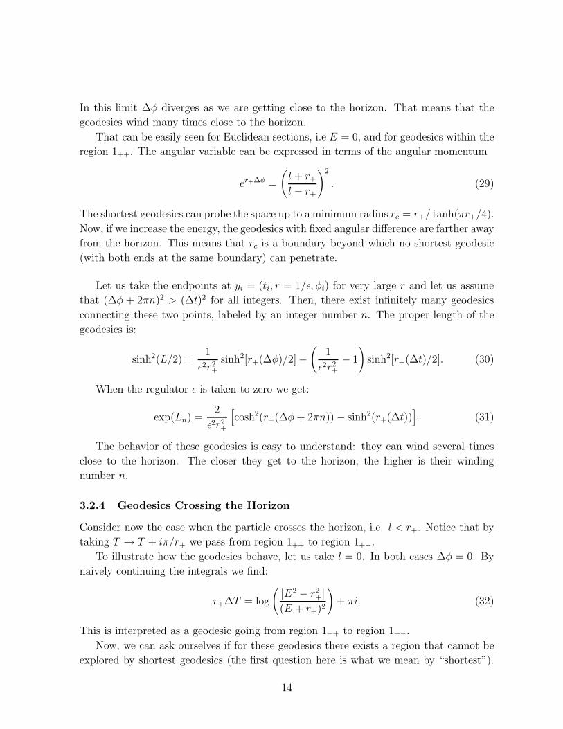
In this limit ∆φ diverges as we are getting close to the horizon. That means that the

geodesics wind many times close to the horizon.

That can be easily seen for Euclidean sections, i.e E = 0, and for geodesics within the

region 1++. The angular variable can be expressed in terms of the angular momentum

er+∆φ =

(

l + r+l − r+

)2

. (29)

The shortest geodesics can probe the space up to a minimum radius rc = r+/ tanh(πr+/4).

Now, if we increase the energy, the geodesics with fixed angular difference are farther away

from the horizon. This means that rc is a boundary beyond which no shortest geodesic

(with both ends at the same boundary) can penetrate.

Let us take the endpoints at yi = (ti, r = 1/ǫ, φi) for very large r and let us assume

that (∆φ + 2πn)2 > (∆t)2 for all integers. Then, there exist infinitely many geodesics

connecting these two points, labeled by an integer number n. The proper length of the

geodesics is:

sinh2(L/2) =1

ǫ2r2+

sinh2[r+(∆φ)/2] −(

1

ǫ2r2+

− 1

)

sinh2[r+(∆t)/2]. (30)

When the regulator ǫ is taken to zero we get:

exp(Ln) =2

ǫ2r2+

[

cosh2(r+(∆φ+ 2πn)) − sinh2(r+(∆t))]

. (31)

The behavior of these geodesics is easy to understand: they can wind several times

close to the horizon. The closer they get to the horizon, the higher is their winding

number n.

3.2.4 Geodesics Crossing the Horizon

Consider now the case when the particle crosses the horizon, i.e. l < r+. Notice that by

taking T → T + iπ/r+ we pass from region 1++ to region 1+−.

To illustrate how the geodesics behave, let us take l = 0. In both cases ∆φ = 0. By

naively continuing the integrals we find:

r+∆T = log

(

|E2 − r2+|

(E + r+)2

)

+ πi. (32)

This is interpreted as a geodesic going from region 1++ to region 1+−.

Now, we can ask ourselves if for these geodesics there exists a region that cannot be

explored by shortest geodesics (the first question here is what we mean by “shortest”).

14

As the geodesics probe inside the horizon, that region has to lie in the interior of the

horizon. Similarly to the case when geodesics end on the same boundary, we start with

E = 0 (∆T = 0). The geodesic touches the horizon and reaches the other boundary.

When we increase the energy for fixed angle, the angular momentum decreases (i.e. the

orbit get closer to the center). To go very close to the singularity we have to take l = 0,

that is the case just explained above.

3.3 Euclidean BTZ Black Hole

The metric of the Euclidean BTZ black hole is defined starting from the Lorentzian one

by continuing to imaginary time:

ds2 = (r2 − r2+)dτ 2 +

dr2

(r2 − r2+)

+ r2dφ2, (33)

where the radial variable goes from r = r+ to infinity and the Euclidean time has period

π/r+ to avoid conical singularities at r = r+. The boundary is a two dimensional torus

parametrized by the Euclidean time and the angular variable. The interior is a solid 3-d

torus, where the points r = r+ form a circle at its center. The manifold is non simple, as

there is more than one geodesic between any two points at the boundary (geodesics can

wind). That is easy to see by considering the uncompactified version, obtained by taking

the angular variable φ non periodic. This space is again the Euclidean AdS (that is best

seen by defining a new variable x2 = r2 − r2+), and, as we know, this space is boundary

rigid. Notice that this example can also be interpreted as AdS at finite temperature,

where the same kind of reasoning applies. The temperature is identified with T = r+/π.

The shortest geodesics reach every point at the interior. This is easily seen because

the sections of constant φ are disks, were the shortest geodesics can connect every two

points. This is a necessary but not sufficient condition for boundary rigidity. Whether

the space is actually boundary rigid is a nontrivial question, which is answered in the

affirmative if the conjecture in Section 5 is true.

3.4 The RP 2 Geon

The RP 2 geon [9] can be obtained from AdS3 by quotienting by the action of a discrete

group generated by:

x1 ± x2 → e±πr+(x1 ± x2). (34)

and x3 → −x3. So, this space is the quotient of the BTZ black hole by a Z2 symmetry.

In region 1 of the BTZ black hole, the geon corresponds to identifying under the

transformation φ → φ + π, η2 → −η2 and t → −t. That is, region 1++ is mapped into

15

region 1+−, i.e. the two exterior regions of the BTZ black hole are interchanged. The

geon is thus a black hole with a single exterior region, isometric to the region 1++ of the

BTZ black hole. Spacelike hypersurfaces are quotients of a cylinder (parametrized by

x ∼ r − r+ and φ) by a freely acting Z2: φ → φ+ π and x → −x. Topologically, this is

RP2 minus the point at r = ∞.

In region 2, the action of the Z2 group is the same as in region 1. In particular, it

interchanges region 2++ with region 2+−. The Penrose diagram is half of the Penrose

diagram of the BTZ black hole, with the upper left part reflected into the lower right

part, and the lower left part into the upper right one.

In region 1 of the BTZ black hole, the geon corresponds to identifying t with t+π, η2

with −η2, and φ with −φ. As in the BTZ black hole, there exist closed timelike curves.

The geodesics ending at the boundary are as in the BTZ black hole, taking into

account that the boundary of 1++ is equivalent to the boundary of region 1+−. So, for

every two points at the boundary, there are geodesics that cross the horizon.

3.5 Euclidean RP 2 Geon

To construct the Euclidean RP 2 geon one takes the Euclidean BTZ, and quotients it by

a Z2 symmetry: φ → φ + π and t → −t. The sections at fixed radius are Klein bottles

(the two dimensional torus with a Z2 identifications). At the horizon, the Klein bottle

degenerates to a circle.

The geodesics connecting points at the boundary can be easily computed by consid-

ering the Euclidean BTZ geodesics, and identifying the points at the boundary as above.

The geodesics of the BTZ black hole can be obtained from the Euclidean AdS3 ones by

the identification φ→ φ+2π. Said in another way, the geodesics of the geon are the same

as in AdS3 when taking into into account the identification between boundary points:

φ→ φ+ π and t→ −t.Let us write the BTZ black hole metric in the form:

ds2 = r2dτ 2 +dr2

1 + r2+ (1 + r2)dφ2, (35)

with periods τ → τ + 2π and φ → φ + 2πr+. To see if the shortest geodesics cover the

whole space we have to compare the distance between two geodesics (see figure 3): the

first one, that is also present in the BTZ, has ∆T = π and ∆φ = 0 [let us call it geodesic

a, joining point (τ = π/2, φ) to (τ = 3π/2, φ)]. The other one, that joins points identified

by the Z2 symmetry, has ∆T = 0 and ∆φ = πr+ [geodesic b, joining point (τ = π/2, φ)

to (τ = π/2, φ+ πr+), that is the Z2 image of (τ = 3π/2, φ)].

16

b

a∆ φ

τ

Figure 3: Two candidates for the shortest geodesic in the geon. Geodesics of type a cover the

whole space, while geodesics of type b do not reach a portion of the space close to the horizon.

The difference in length of the two geodesics is:

la − lb = log

[

4e−πr+

(1 − e−πr+)2

]

. (36)

For small r+ (r+ ≪ 1), the geodesic b is the shortest one. It never reaches the center.

It is easy to see that in this case there is a region inside the geon that cannot be reached

by any shortest geodesics.

For large r+ (r+ ≫ 1), the geodesic a is the shortest. It lies on a constant φ section

of the torus, and, as in the BTZ black hole, covers the whole space.

In the RP 2 case, one can construct a linear combination of two-point correlation

functions that does not receive contributions from the shortest geodesic [9]. So, both

geodesics a and b can be unambiguously determined by boundary data. Equivalently, in

this case, the boundary data are the lengths of all geodesics that lift to minimal-length

ones in the Z2 cover of the RP 2 geon, that is the BTZ black hole. They do probe the

entire space. So, while one cannot reconstruct the geon metric from the spectrum of

shortest geodesics only, more refined boundary data may allow to establish a rigidity

theorem.

17

3.6 Higher-Dimensional Finite-Temperature AdS Black Holes

Now, let us consider the higher-dimensional AdS Black Hole. In this case, there are

two geometries contributing the boundary S1 ×Sd−1: the AdS Schwarzschild Black Hole

(X2 = R2 × Sd−1) and AdS at finite temperature (X1 = S1 × Rd). Unlike in dimension

three, the Euclidean version of these spaces have different topology. In [35, 11], it has been

shown that the dominant geometry at low temperatures is AdS at finite temperature,

while at high temperature the dominant contribution is the black hole. As we have seen

from the previous examples, constant-time geodesics in finite-temperature AdS cover the

whole space, so we expect this space to be boundary rigid. At higher temperature, the

dominant contribution comes from the black hole that, unlike in three dimension, is not

boundary rigid. That can be seen using constant-angle geodesics (then the problem is

reduced to a disk parametrized by time and the radial coordinate).

This is a very interesting case, since the same boundary admits two different geometric

theories, one that is boundary rigid and other that is not. The different geometries have

been identified in [11] with two different phases of the same boundary CFT.

Space Description Boundary Rigid Non Boundary Rigid

Boundary Rigid Cover

Point Particle in AdS3 Constant Time Section X N/A

Zero Temperature X X

Finite Temperature X X

BTZ Black Hole AdS3/Z X X

RP 2 Geon r+ ≪ 1 AdS3/Z2 ⊗S Z X X

RP 2 Geon r+ ≫ 1 AdS3/Z2 ⊗S Z X X

Finite Temperature AdSd AdSd/Z X X

AdSd Black Hole X N/A

Table 1: Summary table of the different examples analysed in this section.

4 Other Bulk Reconstruction Procedures

We have seen that the leading contribution of massive particle propagators reproduces

a unique metric when the manifold is boundary rigid. We have seen several familiar

examples of three dimensional manifolds that are boundary rigid and other manifolds

that are not.

We may ask about other structures that can be obtained from the field theory that

will tell us other information about the Riemannian manifold. Here we review other

procedures that will allow us to partially reconstruct the interior Riemannian manifold.

18

4.1 Dirichlet-to-Neumann Map

Let (M, g) be a Riemannian manifold with boundary ∂M, and consider the follow-

ing problem: find the field φ such that ∆gφ = 0 on M with a given boundary value

φ|∂M = J , where J is a source at the boundary. The Dirichlet-to-Neumann map is the

value of the normal derivative of the solution to the above problem at the boundary:

∂nφ|∂M = ni∂iφ|∂M. In this way we can define a unique function depending on the

sources ∂nφ|∂M(J).

The map is directly related to field theory observables. In the AdS/CFT correspon-

dence, the metric g has a double pole at the boundary ∂M [see Eq. (1)]. This requires

that we regularize the manifold by cutting it off at finite proper distance from the bound-

ary, z = ǫ, as we did in Subsection 2.1. In the dual interpretation in terms of CFT data,

1/ǫ is a UV cutoff of the field theory, needed to properly define composite operators.

The field φ is dual to a CFT operator, O. When the linearized equation of motion of φ

is ∆gφ = 0, then the operator O has conformal dimension ∆ = d = dim ∂M. The field

φ(z, x) can be expanded as [11, 12, 13]

φ(ǫ, x) = φ0(x) + ǫ2φ2(x) + ...+ ǫd log ǫ2φd(x) + ǫdψd(ǫ, x). (37)

The coefficients φ2, ..φd are known, local functions of φ0(x) and ψd(ǫ, x) = ψd(0, x)+O(ǫ2).

So, in Eq. (37) there are two unknown functions: φ0(x) and ψd(ǫ, x). The Dirichlet-to-

Neumann data allow to fix them both. In the limit ǫ → 0, φ0(0) is identified with the

source I of the the operator O, while ψd(0, x) becomes proportional to the VEV of the

operator O. More precisely [11, 12, 13],

ψd(0, x) = 4〈0|O(x) exp(

−∫

∂MIO)

|0〉. (38)

The inverse problem5 consists in extracting information about the Riemannian man-

ifold from the Dirichlet-to-Neumann map ∂nφ|∂M(J).

It is conjectured that the for manifolds of dimension dim(M) > 2 the Dirichlet-

to-Neumann map determines the Riemannian manifold uniquely (for dimension two it

determines uniquely the conformal class of the metric). It has been proved by Uhlmann

and collaborators [27, 28, 29, 30] that the Dirichlet-to-Neumann map determines the Rie-

mannian metric for real-analytic manifolds of dimension dim(M) > 2 and the conformal

structure for C∞ manifolds and dim(M) = 2.

5This inverse problem has appeared in several fields. It was proposed by Calderon [22] in 1980,

motivated by geophysical prospection. It also appears in Electrical Impedance Tomography (EIT) in

trying to obtain the conductivity of a medium by making voltage and currents measurements on the

boundary.

19

4.2 Scattering Relation

Imagine a geodesic that starts and ends at the boundary of a Riemannian manifold.

The scattering relation is a function that, for a starting point and initial velocity of a

geodesic at the boundary, gives the final point and the final velocity at the boundary:

α(xi, vi) = (xf , vf). For that map to be well defined, we demand that the Riemannian

manifold is non-trapping, i.e. that each maximal geodesic is finite. The scattering relation

is an involution (α2 is the identity).

In the dual field theory, one may think of obtaining this relation from a two-point

correlator of a dimension-∆ ≫ 1 operator as follows.

The correlator of two (bare) operators in the regularized theory with cutoff ǫ is, thanks

to Eq. (4),

〈O(x)O(y)〉ǫ ∝ exp[−∆Dmin(x, y)/L]. (39)

We can convolute 〈O(x)O(y)〉ǫ with a function f(x), localized around xi within an un-

certainty δ:∫

∂Mǫ

f(x)〈O(x)O(y)〉ǫ. (40)

This function also localizes the momentum components along the boundary, p = −i∂/∂x,within an uncertainty 1/δ around a central value pi. In the geodesic approximation, the

mass-shell condition L2∑d+1m=1 pmp

m = ∆(∆ − d) = m2L2 holds. So, we also know the

normal component of the momentum, within an uncertainty 1/δ. Whenever pi ≫ 1/δ,

and the boundary is sufficiently smooth, we may reasonably approximate the result of

the convolution by assigning an initial position xi and initial velocity vi = pi/m to the

geodesic∫

∂Mǫ

f(x)〈O(x)O(y)〉ǫ ≈ exp[−∆Dvi(xi, y)/L]. (41)

Clearly, in this approximation, the two-point function is nonzero only for a specific value

of y, to wit: the final point xf . Eq. (41) also uniquely defines the final velocity vf

(by convoluting it with an approximate eigenstate of the final momentum) hence the

scattering relation.

The problem with this procedure is that it does not give an exact dispersion relation,

but only an approximate one. This is because Eq. (41) is exact only in the classical

limit. Even within the semiclassical approximation, Eq. (41) is contaminated by extremal

trajectories beginning near (xi, vi). To be concrete, imagine the case that two trajectories

join the points xi, xf ; one with initial velocity vi, the other with initial velocity wi. Both

trajectories contribute to Eq. (41). To estimate the contribution of the second, denote

by f the Fourier transform of f . For f Gaussian of width δ we have, approximately,

20

f(mv) ≈ exp[−δ∆2(v − vi)2/2L2]; so, Eq. (41) becomes, with obvious notations

∫

∂Mǫ

f(x)〈O(x)O(y)〉ǫ ≈ exp[−∆Dvi(xi, y)/L]+exp[−δ∆2(wi−vi)

2/2L2−∆Dwi(xi, y)/L].

(42)

The second contribution can be neglected only if

exp[−δ∆2(wi − vi)2/2L2 − ∆Dwi

(xi, y)/L+ ∆Dvi(xi, y)/L] ≪ 1. (43)

This restricts the validity of Eq. (41) to manfolds which, even though non-simple, do not

have geodesics with lenght too close to the minimizing one. To make precise statements

on non-minimizing geodesics, we need additional information on the CFT, as explained

later in Subsection 4.4 and in the Conclusions.

The inverse problem is whether the scattering relation determines the metric. In the

case that the manifold is simple the scattering relation is equivalent to the boundary

distance function for the two points at the boundary [15]. It has been shown in [21]

that in two dimensional simple manifolds the Dirichlet-to-Neumann map is determined

by the scattering relation. So in this case the scattering relation, the hodograph and the

Dirichlet-to-Neumann map are related.

4.3 Bulk to Boundary Functions

A complete information about the metric on the manifold is given by the bulk to boundary

Green function for very massive fields. Again, in the limit of very high mass this function

is very well approximated by the distance rx(y) between a point at the interior of the

manifold x ∈ M and a point at the boundary y ∈ ∂M. Now let us consider the function

R that assigns to every point x ∈ M its boundary distance function R : x ∈ M → rr ∈L∞(∂M), where L∞(∂M) is the space with the norm:

||r|| = supz∈(∂M)|r(z)|. (44)

Let us call R(M) the set of all boundary distance functions. In [31] it is shown that

one can construct a differential structure and a metric on the set of the boundary distance

functions such that it becomes isometric to the original Riemannian manifold.

To see how it works, let us consider first the case of geodesically regular manifolds

(there is a unique geodesic between any two points in the bulk, and the geodesic goes to

the boundary). Then we will consider the general case. Take two points x and x′ in the

interior of M and compute the function:

f : ∂M → R+,

y 7→ |rx(y) − rx′(y)|. (45)

21

Using the triangular inequality one can easily see that d(x, x′) ≥ f(y) for all points y.

If in addition the manifold is regular, there is a unique geodesic that joins the points x

and x′ and that goes till the boundary (let us call this point at the boundary yc). At this

point the inequality is saturated: d(x, x′) ≥ f(y). As there is only one geodesic (regular

manifold) that means that the distance between the two points is just the maximum of

f(y).

That is: we can read what is the distance between any two points inside from the

bulk to boundary function.

A direct extension of this reasoning will be to consider the case when there are several

geodesics between the points x and x′ (i.e one is the shortest and the other wind around

the manifold). Then there are several local maxima. The lower of these maxima is the

distance (measured by the shortest geodesic). The only requirement is that the geodesics

arrive to the boundary. The proof of how the metric is reconstructed from the bulk to

boundary functions for general manifolds can be found in [31].

So, if we know the bulk-to-boundary distance, we can easily reconstruct the bulk met-

ric. Unfortunately, the holographic interpretation of this quantity is rather mysterious.

In specific theories, as SU(N), N = 4 super Yang-Mills, one may be able to extract it from

expectation values of, say, TrFµνFµν , computed on a one-instanton background [33, 34].

The actual implementation of this program on a generic manifold is still unclear to us.

4.4 Spectral Boundary Data

Now, let us consider a different type of data. They are obtained from a differential

operator (it must be elliptic, so we must work in Euclidean space) of the form:

D = − 1√g∂i(

√ggij∂j) + V (46)

where V is an arbitrary functions on M. This operator can be obtained from an action:

S =∫

f√g[

(∂φ)2 + V φ2]

(47)

that can be interpreted as the action of a massive particle φ with a position-dependent

“mass” m2 = V . Notice that if we have a dimensional reduction of the form M×M′ to

M with a warped metric, the warp factor can always be interpreted as a modification of

the potential.

Now, let us consider the Dirichlet problem on M, i.e. φ|∂M = 0. The boundary

spectral data is the collection of all the eigenvalues λk and the normal derivatives of the

eigenfunctions at the boundary ∂nφk|∂M = ni∂iφk|∂M.

In [36, 31] it is show how the spectral data determines uniquely the manifold M, the

metric g and the variable mass V . It is shown that the boundary spectral data determines

22

the set of boundary distance functions. As we have shown in the previous paragraph this

also defines the metric.

To obtain these data from a boundary CFT, we need additional assumptions, either

on the bulk manifold or on the analytic structure of the CFT. For instance, if the space-

time manifold has a time-like global Killing vector, then we can reinterpret M as its

constant-time section. Then the eigenvalues λk are determined by the conformal weights

of the CFT [11].

For a generic bulk manifold, this interpretation is not possible. Nevertheless, spectral

boundary data can be obtained if the two-point correlator of CFT operators of arbitrary

dimension ∆, F (∆, x, y) ≡ 〈O∆(x)O∆(y)〉, is a known analytic function of ∆. In this

case, the poles of this function determine the λk. Of course, analyticity in ∆ is a rather

tall order on a generic CFT!

5 Summary, Conclusions, Speculations

In Section 3 we found that the Euclidean geon is in some cases non-rigid, yet its met-

ric can be determined if we know all its boundary geodesics, not only the minimizing

(shortest) ones. Indeed, in all examples we gave, manifest non-rigidity was associated to

the existence of a region unreachable by shortest geodesics. That limitation was crucial.

Longer geodesics, with nonzero winding number, can reach all points inside all spaces

studied in Section 3. So, neither the AdS3 point particle at finite temperature, nor its

t = 0 section, nor the small (r+ ≪ 1) geon possess regions that cannot be reached by

some geodesic. If one can find an unambiguous way to determine the length of non-

minimal geodesics from boundary data, then these spaces may be boundary rigid after

all. They all share one common property: they are quotients by discrete isometries of a

boundary rigid space: AdS3. This leads us to the following conjecture:

Quotients of boundary rigid manifolds by discrete isometries are also boundary

rigid if they have the same scattering relation.

In stating the conjecture, we used the fact that the natural way to obtain the spectrum

of all boundary geodesics is through the scattering relation.

If true, this conjecture would give a concrete, computationally effective way to recon-

struct a bulk metric from simple holographic data.

So, it is important to see if the scattering relation can be determined by the CFT

correlators. As we saw in Subsection 4.2, the “physical” way of obtaining it is only

approximate. To do better, we must assume some additional analyticity property in ∆

for the two-point correlators of the CFT. Specifically, if F (∆, x, y), defined in the previous

23

subsection, is analytic for ∆ ≫ 1, then one can us the geodesic approximation to arrive

at

F (∆, x, y) =∑

i

consti {1 +O[L/∆Di(x, y)]} exp[−∆Di(x, y)/L]. (48)

Here the sum extends to all geodesics between the boundary points x and y. Since

F (∆, x, y) is analytic in ∆, its inverse Laplace transform, F (t, x, y) contains delta func-

tions located precisely at t = ∆i(x, y)

F (t, x, y) =∑

i

consti δ[t− ∆i(x, y)] + .... (49)

The ellipsis denote less singular terms.

Finally, we must remember that in the case when the CFT is a gauge theory, there are

additional non-local observables with a simple geometric interpretation in the holographic

dual. One such observable is the Wilson loop. In particular, the correlator of two Wilson

loops is ∝ exp(−Sm), where Sm is the minimal surface between the two loops [37]. This

leads to another inverse problem; namely: when is it possible to reconstruct the metric

of a manifold with a known spectrum of minimal surfaces in between boundary loops?

Acknowledgments

We would like to thank D. Berenstein, M. Kleban, J. Maldacena, and especially G.

Uhlmann for helpful discussions. The work of M.P. is supported in part by NSF through

grants PHY-0070787 and PHY-0245068. R.R. is supported by DOE under grant DE-

FG02-90ER40542.

References

[1] G. ’t Hooft, arXiv:gr-qc/9310026; L. Susskind, J. Math. Phys. 36, 6377 (1995)

[arXiv:hep-th/9409089].

[2] R. Bousso, Class. Quant. Grav. 17, 997 (2000) [arXiv:hep-th/9911002].

[3] J. M. Maldacena, Adv. Theor. Math. Phys. 2, 231 (1998) [Int. J. Theor. Phys. 38,

1113 (1999)] [arXiv:hep-th/9711200].

[4] O. Aharony, S. S. Gubser, J. M. Maldacena, H. Ooguri and Y. Oz, Phys. Rept. 323,

183 (2000) [arXiv:hep-th/9905111].

[5] L. Susskind and N. Toumbas, Phys. Rev. D 61, 044001 (2000)

[arXiv:hep-th/9909013]; S. B. Giddings and M. Lippert, Phys. Rev. D 65,

24

024006 (2002) [arXiv:hep-th/0103231]; B. Freivogel, S. B. Giddings and M. Lippert,

Phys. Rev. D 66, 106002 (2002) [arXiv:hep-th/0207083].

[6] P. Kraus, H. Ooguri and S. Shenker, Phys. Rev. D 67, 124022 (2003)

[arXiv:hep-th/0212277]; T. S. Levi and S. F. Ross, Phys. Rev. D 68, 044005

(2003) [arXiv:hep-th/0304150]; L. Fidkowski, V. Hubeny, M. Kleban and S. Shenker,

arXiv:hep-th/0306170.

[7] V. Balasubramanian and S. F. Ross, Phys. Rev. D 61, 044007 (2000)

[arXiv:hep-th/9906226].

[8] M. Banados, C. Teitelboim and J. Zanelli, Phys. Rev. Lett. 69, 1849 (1992)

[arXiv:hep-th/9204099];

M. Banados, M. Henneaux, C. Teitelboim and J. Zanelli, Phys. Rev. D 48, 1506

(1993) [arXiv:gr-qc/9302012].

[9] J. Louko and D. Marolf, Phys. Rev. D 59, 066002 (1999) [arXiv:hep-th/9808081];

J. Louko, D. Marolf and S. F. Ross, Phys. Rev. D 62, 044041 (2000)

[arXiv:hep-th/0002111].

[10] S. S. Gubser, I. R. Klebanov and A. M. Polyakov, Phys. Lett. B 428, 105 (1998)

[arXiv:hep-th/9802109]

[11] E. Witten, Adv. Theor. Math. Phys. 2, 253 (1998) [arXiv:hep-th/9802150].

[12] M. Henningson and K. Skenderis, JHEP 9807, 023 (1998) [arXiv:hep-th/9806087].

[13] S. de Haro, S. N. Solodukhin and K. Skenderis, Commun. Math. Phys. 217, 595

(2001) [arXiv:hep-th/0002230].

[14] C. B. Croke, Rigidity Theorems in Riemannian geometry,

http://www.math.upenn.edu∼ccroke/papers.html.

[15] R. Michel, Invent. Math. 65, 71 (1981).

[16] C. B. Croke, J. Diff. Geom. 33, 445 (1991).

[17] L. Pestov and A. Sharafutdinov, Sibirskii Math. Zhurnal 29, 114 (1988).

[18] V. A. Sharafutdinov, Siberian Math. J. 33 533 (1993).

[19] M. Lassas, V. Sharafutdinov, G. Uhlmann, Math. Ann. 325, 767 (2003).

[20] C. B. Croke, N. S. Dairbekov, V. A. Sharafutdinov, Trans. Amer. Math. Soc. 352,

3937 (2000).

25

[21] L. Pestov, G. Uhlmann, The Boundary Distance Function and the Dirichlet-to-

Neumann map, (private communication).

[22] C. B. Croke, Comment. Math. Helv. 65, 150 (1990).

[23] M. Gromov, J. Differential Geom. 18, 1 (1983).

[24] G. Besson, G. Courtois, S. Gallot, Ergodic Theory Dynam. Systems 16, 623 (1996).

[25] L. Andersson, M. Dahl, R. Howard, Trans. Amer. Math. Soc. 348, 2307 (1996).

[26] A.P. Calderon, Seminar on Numerial Analysis and its Applications to Continuum

Physics, Soc. Brasileira de Matematica, Rio de Janeiro (1980), 65.

[27] J. Lee, G. Uhlmann, Comm. Pure Appl. Math. 42, 1097 (1989).

[28] M. Lassas, G. Uhlmann, Ann. Sci. cole Norm. Sup. 4 34, no. 5, 771 (2001).

[29] M. Lassas, M. Taylor, G. Uhlmann, Comm. in Analysis and Geometry, 19, 207

(2003).

[30] G. Uhlmann, On the Local Dirichlet-to-Neumann Map, to appear in Springer-Verlag,

Lecture Notes in Mathematics.

[31] A. Katchalov, Y. Kurylev, M. Lassas, Inverse boundary spectral problems, Chapman

and Hall, Monographs and Surveys in Pure and Applied Mathematics 123 (2001).

[32] S. Hemming, E. Keski-Vakkuri and P. Kraus, JHEP 0210, 006 (2002)

[arXiv:hep-th/0208003].

[33] V. Balasubramanian, P. Kraus, A. E. Lawrence and S. P. Trivedi, Phys. Rev. D 59,

104021 (1999) [arXiv:hep-th/9808017].

[34] M. Bianchi, M. B. Green, S. Kovacs and G. Rossi, JHEP 9808, 013 (1998)

[arXiv:hep-th/9807033].

[35] S. W. Hawking and D. N. Page, Commun. Math. Phys. 87, 577 (1983).

[36] M.I. Belishev, Y.V. Kurylev, Comm. PDE 17, 767 (1992).

[37] S. J. Rey and J. T. Yee, Eur. Phys. J. C 22, 379 (2001) [arXiv:hep-th/9803001]

J. M. Maldacena, Phys. Rev. Lett. 80, 4859 (1998) [arXiv:hep-th/9803002].

S. J. Rey, S. Theisen and J. T. Yee, Nucl. Phys. B 527, 171 (1998)

[arXiv:hep-th/9803135]

D. Berenstein, R. Corrado, W. Fischler and J. M. Maldacena, Phys. Rev. D 59,

26

105023 (1999) [arXiv:hep-th/9809188]

N. Drukker, D. J. Gross and H. Ooguri, Phys. Rev. D 60, 125006 (1999)

[arXiv:hep-th/9904191].

27