Boundary Number Systems Table of Contents Boundary Number Systems William Bricken January 2001 Table...

1

Boundary Number SystemsWilliam Bricken

January 2001

Table of Contents

ABSTRACT

Boundary mathematics represents abstract mathematical concepts using empty and full containers, as

opposed to tokens in conventional systems. We examine several boundary number systems in depth.

Conway numbers are bootstrapped into existence by the act of partitioning the void. They form a

comprehensive system spanning all conventional types of numbers. As well, they provide sufficient

structure to define algebraic transformations of infinities. Spencer-Brown numbers confound

operations and objects, representing both by configurations of a single type of container. This was the

first system based entirely on boundary concepts. Kauffman numbers use depth of nesting of containers

as a type of positional notation. Algebraic operations are trivial; addition is sharing a space,

multiplication is direct substitution of one form into another. Computational effort occurs after all

operations are completed, in the course of standardizing forms to a canonical ground, which is then

interpreted as a number. Bricken numbers convert Kauffman numbers into graphs that permit

parallel processing. James numbers use three types of containers to represent algebraic and

transcendental forms. The concepts of cardinality and inversion are simplified and generalized. A new

imaginary, ln-1, provides access to new computational tools.

CONTENTS

Boundary Number Systems

History of Integers

Types of Numbers

The Numerical/Measurement Hierarchy

Integers as Sets

Some Exotic Varieties of Numbers


2

Conway Numbers (Surreal Numbers)

Partitioning Nothing

Ordering and Equality

Building from Zero

Building from One

Number Forms

ordinal

negative integer

fraction

real

Conway Operators

addition

negation

multiplication

division

Infinities and Infinitessimals

Imaginary Star

Commentary

Spencer-Brown Numbers

Spencer-Brown Arithmetic (Parenthesis Version)

Reduction Rules

involution

distribution

Operations

addition

multiplication

power

Confounding Objects and Operations

Computation

Void Transforms

Inconsistency

3

Kauffman Numbers

Kauffman Arithmetic (String Version)

Canonical Transformations

commutativity

power

distribution

Operations

addition

multiplication

Inverse Operations

Kauffman Arithmetic (Molecular Version)

Commentary

Bricken Graph-numbers

Definitions

Parallel Standardization Rules

Group

Coalesce

Multiple Representations

18

Numerical Operators

Addition

Subtraction

Plus-cancel

Multiplication

Cross-connect

Division

Multiply-cancel

Stacking

Peano Axioms for Arithmetic

Peano Axioms in Boundary Form

4

James Numbers

Boundary Units

Boundary Operators

Integers

Algebraic Operations

addition

multiplication

power

Inverse Operations

subtraction

division

root

Reduction Rules (Axiomatic basis)

involution

distribution

inversion

Algebraic Proof

The Form of Numbers

The Form of Numerical Computation

Logarithms

Generalized Inverse

subtraction

division

root

log

Dominion

Inverse Theorems

inverse collection

inverse cancellation

inverse promotion

Examples

Generalized Cardinality

multiple reference

negative cardinality

fractional cardinality

Broadening the Distributive Axiom

James Calculus Unit Combinations

Stable Forms

5

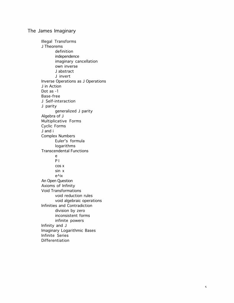
The James Imaginary

Illegal Transforms

J Theorems

definition

independence

imaginary cancellation

own inverse

J abstract

J invert

Inverse Operations as J Operations

J in Action

Dot as -1

Base-free

J Self-interaction

J parity

generalized J parity

Algebra of J

Multiplicative Forms

Cyclic Forms

J and i

Complex Numbers

Euler's formula

logarithms

Transcendental Functions

e

P I

cos x

sin x

e^ix

An Open Question

Axioms of Infinity

Void Transformations

void reduction rules

void algebraic operations

Infinities and Contradiction

division by zero

inconsistent forms

infinite powers

Infinity and J

Imaginary Logarithmic Bases

Infinite Series

Differentiation

6


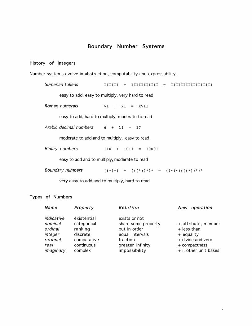
History of Integers

Number systems evolve in abstraction, computability and expressability.

Sumerian tokens IIIIII + IIIIIIIIIII = IIIIIIIIIIIIIIIII

easy to add, easy to multiply, very hard to read

Roman numerals VI + XI = XVII

easy to add, hard to multiply, moderate to read

Arabic decimal numbers 6 + 11 = 17

moderate to add and to multiply, easy to read

Binary numbers 110 + 1011 = 10001

easy to add and to multiply, moderate to read

Boundary numbers ((*)*) + (((*))*)* = ((*)*)(((*))*)*

very easy to add and to multiply, hard to read

Types of Numbers

Name Property Re la t ion New operation

indicative existential exists or not

nominal categorical share some property + attribute, member

ordinal ranking put in order + less than

integer discrete equal intervals + equality

rational comparative fraction + divide and zero

real continuous greater infinity + compactness

imaginary complex impossibility + i, other unit bases

7

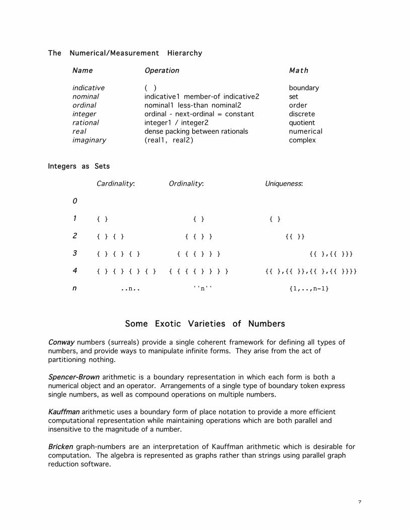
The Numerical/Measurement Hierarchy

Name Operation Math

indicative ( ) boundary

nominal indicative1 member-of indicative2 set

ordinal nominal1 less-than nominal2 order

integer ordinal - next-ordinal = constant discrete

rational integer1 / integer2 quotient

real dense packing between rationals numerical

imaginary (real1, real2) complex

Integers as Sets

Cardinality: Ordinality: Uniqueness:

0

1 { } { } { }

2 { } { } { { } } {{ }}

3 { } { } { } { { { } } } {{ },{{ }}}

4 { } { } { } { } { { { { } } } } {{ },{{ }},{{ },{{ }}}}

n ..n.. ''n'' {1,..,n-1}

Some Exotic Varieties of Numbers

Conway numbers (surreals) provide a single coherent framework for defining all types of

numbers, and provide ways to manipulate infinite forms. They arise from the act of

partitioning nothing.

Spencer-Brown arithmetic is a boundary representation in which each form is both a

numerical object and an operator. Arrangements of a single type of boundary token express

single numbers, as well as compound operations on multiple numbers.

Kauffman arithmetic uses a boundary form of place notation to provide a more efficient

computational representation while maintaining operations which are both parallel and

insensitive to the magnitude of a number.

Bricken graph-numbers are an interpretation of Kauffman arithmetic which is desirable for

computation. The algebra is represented as graphs rather than strings using parallel graph

reduction software.

8

The James Calculus uses three boundaries to shift the representation of numbers between

exponential and logarithmic forms. This mechanism generalizes the concepts of cardinality and

inverse operations. A new imaginary imparts phase structure on numbers, and permits

computation without inverses. This system is discussed in depth as an example of novel

mathematical thinking, and provides an astonishing link between imaginary surreals and

function inversion.


Boundary number systems can be characterized by these features:

• semantic use of the void

• semantic use of spatial juxtaposition

• containers as tokens

• object/process confounding

• implicit commutativity and associativity

• a diversity of standard algebraic operations condensed into a few axioms

• computational effort in form standardization rather than addition or multiplication

The last feature is an historical reversion using efficient computational techniques. Place

notation and algebraic operations (introduced in the sixteenth century) shift the computational

effort from one-to-one correspondence to abstract transformation of structure based on rules.

Boundary numbers make the traditional algebraic operations {+,-,*,/,^,root} trivial to

implement; the computational effort is shifted to converting a given form into a canonical

representation. However, in contrast to conventional decimal and binary numbers, boundary

numbers can be read as a computational result at any time during the canonicalization process.

An advantage of the boundary notation is that it can condense a diversity of standard algebraic

operations and transformations into three simple axiomatic rules.

9

Conway Numbers (Surreal Numbers)

John Conway (and later Don Knuth) constructed all known types of numbers from the simplest

possible beginning, making a distinction in the void. The generative definition is

A number is a partitioned set of prior numbers, {L|G},

such that no member of L is greater than or equal to any member of G.

The initial number is when L and G are both void: { | }

The set L contains lesser numbers, while the set G contains greater numbers. Both L and G can

be void, that is, they can be collections without any members.

Let xL be an arbitrary member of L, and xG be an arbitrary member of G.

x = {xL|xG} such that no xL >= any xG

i.e. every xL < every xG

By definition, no xL >= any xG is true whenever L is empty, even if G is empty. When there

are no members of L, every member is less than any in G.

Partitioning Nothing

"Before we have any numbers, we have a certain set of numbers, namely the empty set, {}."

-- John H. Conway

Base: { | } empty partitions of the empty set

Generator: every partition of the set of prior numbers

The empty set is not the base of the system, rather the act of partitioning is the base.

Partitioning creates the first distinction, which serves as sufficient structure to build all

numerical forms and operations.

The conventional names of numbers can be assigned to Conway numbers. For example:

{ | } = 0

We can test if this first partition is a number:

Is { | } a number?

every xL < every xG? yes since there are no xL

10

Ordering and Equality

We next define the ordering of numbers. A Conway number is defined by comparing the

members of each partition. Ordering and equality are defined by comparing all the members in

a partition of one number to the value of another number (not to its partitions).

Two Conway numbers are ordered

x >= y when no xG <= y and no yL >= x

i.e. every xG > y and every yL < x

Example: let x = {0,1|2,3} and y = {-1|1}.

To determine the ordering, we will need to know the value of each of these numbers. To be

shown later, x = 1 1/2 and y = 0.

Is x >= y?

every xG > y xG = {2,3}, y = 0 trueevery yL < x yL = -1, x = 0 true

therefore {0.1|2,3} >= {-1|1}

Two Conway numbers are strictly ordered

x > y when x >= y and not y >= x

i.e. all xG > y, all yL < x, some xL < y, some yG > x

Two Conway numbers are equal

x = y when x >= y and y >= x

i.e. all xG > y, all xL < y, all yL < x, all yG > x

Example:

Is { | } >= { | } is 0 >= 0? x=0 y=0

every xG > 0 and every yL < 0? yes since there are no xG or yL

By symmetry y >= x, thus 0 = 0

Now we will determine how to find the conventional value of a Conway number, and how to

identify the canonical form of a Conway number.

11

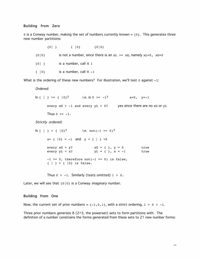
Building from Zero

0 is a Conway number, making the set of numbers currently known = {0}. This generates three

new number partitions:

{0| } { |0} {0|0}

{0|0} is not a number, since there is an xL >= xG, namely xL=0, xG=0

{0| } is a number, call it 1

{ |0} is a number, call it -1

What is the ordering of these new numbers? For illustration, we'll test 0 against -1:

Ordered:

Is { | } >= { |0}? i.e. is 0 >= -1? x=0, y=-1

every xG > -1 and every yL < 0? yes since there are no xG or yL

Thus 0 >= -1.

Strictly ordered:

Is { | } > { |0}? i.e. not(-1 >= 0)?

x= { |0} = -1 and y = { | } =0

every xG > y? xG = { }, y = 0 trueevery yL < x? yL = { }, x = -1 true

-1 >= 0, therefore not(-1 >= 0) is false,{ | } > { |0} is false.

Thus 0 > -1. Similarly (tests omitted) 1 > 0.

Later, we will see that {0|0} is a Conway imaginary number.

Building from One

Now, the current set of prior numbers = {-1,0,1}, with a strict ordering, 1 > 0 > -1.

Three prior numbers generate 8 (2^3, the powerset) sets to form partitions with. The

definition of a number constrains the forms generated from these sets to 21 new number forms:

12

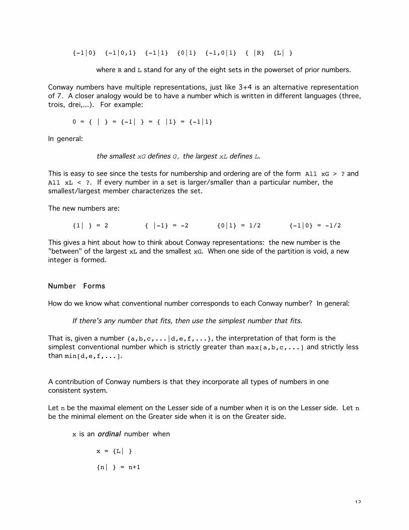
{-1|0} {-1|0,1} {-1|1} {0|1} {-1,0|1} { |R} {L| }

where R and L stand for any of the eight sets in the powerset of prior numbers.

Conway numbers have multiple representations, just like 3+4 is an alternative representation

of 7. A closer analogy would be to have a number which is written in different languages (three,

trois, drei,...). For example:

0 = { | } = {-1| } = { |1} = {-1|1}

In general:

the smallest xG defines G, the largest xL defines L.

This is easy to see since the tests for numbership and ordering are of the form All xG > ? and

All xL < ?. If every number in a set is larger/smaller than a particular number, the

smallest/largest member characterizes the set.

The new numbers are:

{1| } = 2 { |-1} = -2 {0|1} = 1/2 {-1|0} = -1/2

This gives a hint about how to think about Conway representations: the new number is the

"between" of the largest xL and the smallest xG. When one side of the partition is void, a new

integer is formed.

Number Forms

How do we know what conventional number corresponds to each Conway number? In general:

If there's any number that fits, then use the simplest number that fits.

That is, given a number {a,b,c,...|d,e,f,...}, the interpretation of that form is the

simplest conventional number which is strictly greater than max[a,b,c,...] and strictly less

than min[d,e,f,...].

A contribution of Conway numbers is that they incorporate all types of numbers in one

consistent system.

Let n be the maximal element on the Lesser side of a number when it is on the Lesser side. Let nbe the minimal element on the Greater side when it is on the Greater side.

x is an ordinal number when

x = {L| }

{n| } = n+1

13

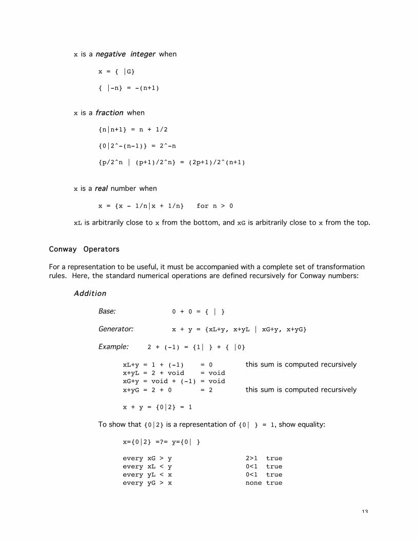
x is a negative integer when

x = { |G}

{ |-n} = -(n+1)

x is a fraction when

{n|n+1} = n + 1/2

{0|2^-(n-1)} = 2^-n

{p/2^n | (p+1)/2^n} = (2p+1)/2^(n+1)

x is a real number when

x = {x - 1/n|x + 1/n} for n > 0

xL is arbitrarily close to x from the bottom, and xG is arbitrarily close to x from the top.

Conway Operators

For a representation to be useful, it must be accompanied with a complete set of transformation

rules. Here, the standard numerical operations are defined recursively for Conway numbers:

Addition

Base: 0 + 0 = { | }

Generator: x + y = {xL+y, x+yL | xG+y, x+yG}

Example: 2 + (-1) = {1| } + { |0}

xL+y = 1 + (-1) = 0 this sum is computed recursivelyx+yL = 2 + void = voidxG+y = void + (-1) = voidx+yG = 2 + 0 = 2 this sum is computed recursively

x + y = {0|2} = 1

To show that {0|2} is a representation of {0| } = 1, show equality:

x={0|2} =?= y={0| }

every xG > y 2>1 trueevery xL < y 0<1 trueevery yL < x 0<1 trueevery yG > x none true

14

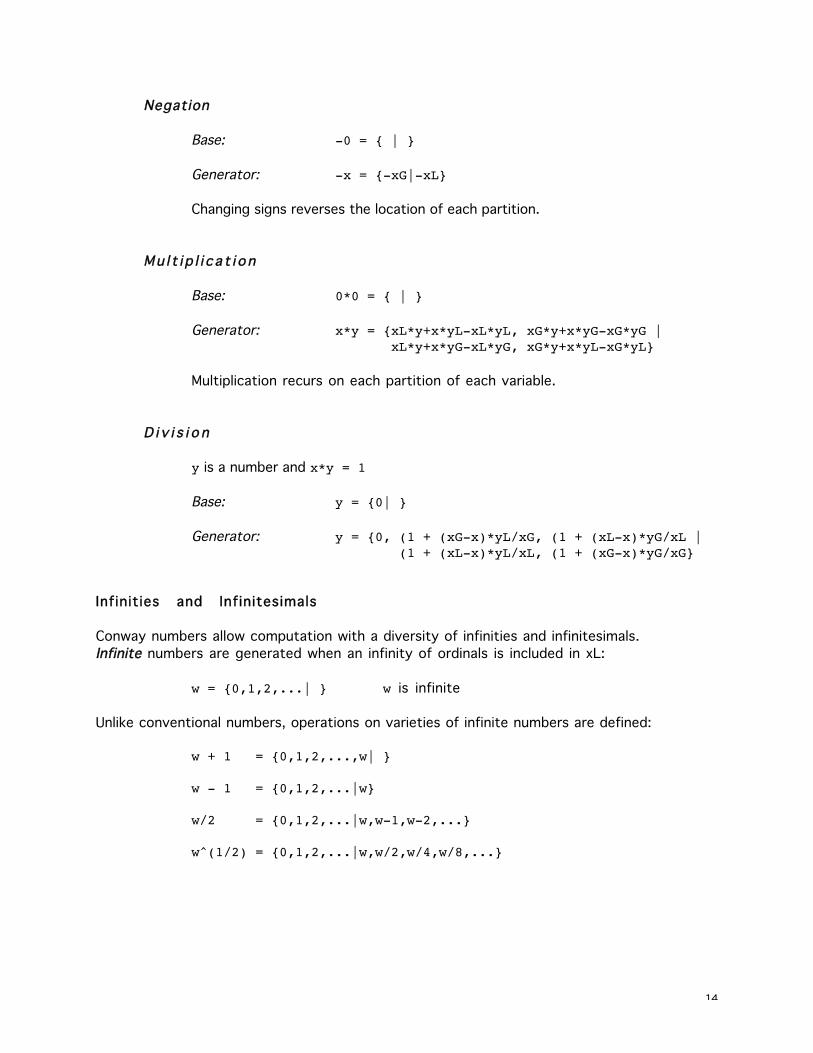
Negation

Base: -0 = { | }

Generator: -x = {-xG|-xL}

Changing signs reverses the location of each partition.

Mu l t i p l i c a t i o n

Base: 0*0 = { | }

Generator: x*y = {xL*y+x*yL-xL*yL, xG*y+x*yG-xG*yG | xL*y+x*yG-xL*yG, xG*y+x*yL-xG*yL}

Multiplication recurs on each partition of each variable.

D i v i s i o n

y is a number and x*y = 1

Base: y = {0| }

Generator: y = {0, (1 + (xG-x)*yL/xG, (1 + (xL-x)*yG/xL | (1 + (xL-x)*yL/xL, (1 + (xG-x)*yG/xG}

Infinities and Infinitesimals

Conway numbers allow computation with a diversity of infinities and infinitesimals.

Infinite numbers are generated when an infinity of ordinals is included in xL:

w = {0,1,2,...| } w is infinite

Unlike conventional numbers, operations on varieties of infinite numbers are defined:

w + 1 = {0,1,2,...,w| }

w - 1 = {0,1,2,...|w}

w/2 = {0,1,2,...|w,w-1,w-2,...}

w^(1/2) = {0,1,2,...|w,w/2,w/4,w/8,...}

15

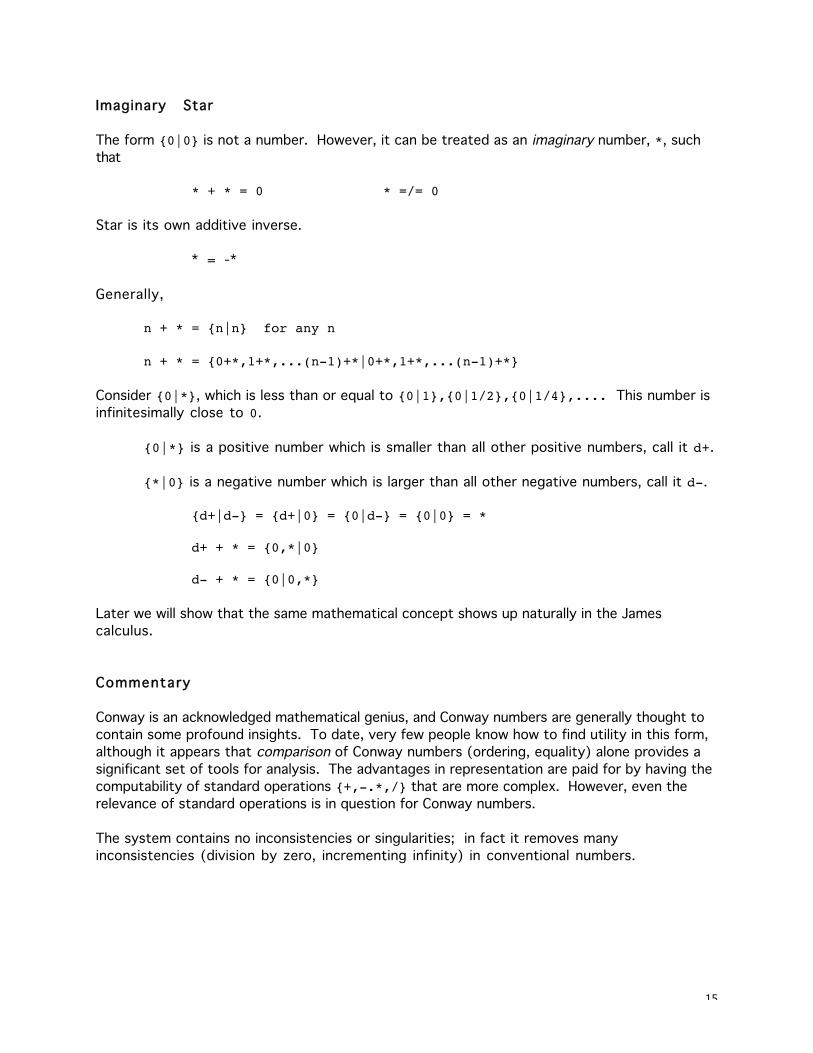
Imaginary Star

The form {0|0} is not a number. However, it can be treated as an imaginary number, *, such

that

* + * = 0 * =/= 0

Star is its own additive inverse.

* = -*

Generally,

n + * = {n|n} for any n

n + * = {0+*,1+*,...(n-1)+*|0+*,1+*,...(n-1)+*}

Consider {0|*}, which is less than or equal to {0|1},{0|1/2},{0|1/4},.... This number is

infinitesimally close to 0.

{0|*} is a positive number which is smaller than all other positive numbers, call it d+.

{*|0} is a negative number which is larger than all other negative numbers, call it d-.

{d+|d-} = {d+|0} = {0|d-} = {0|0} = *

d+ + * = {0,*|0}

d- + * = {0|0,*}

Later we will show that the same mathematical concept shows up naturally in the James

calculus.

Commentary

Conway is an acknowledged mathematical genius, and Conway numbers are generally thought to

contain some profound insights. To date, very few people know how to find utility in this form,

although it appears that comparison of Conway numbers (ordering, equality) alone provides a

significant set of tools for analysis. The advantages in representation are paid for by having the

computability of standard operations {+,-.*,/} that are more complex. However, even the

relevance of standard operations is in question for Conway numbers.

The system contains no inconsistencies or singularities; in fact it removes many

inconsistencies (division by zero, incrementing infinity) in conventional numbers.

16

References for further study:

J.H. Conway (1976) On Numbers and Games, Academic Press

An academic introduction to Conway numbers. Contains some of the material in the next

reference, but presented more succinctly.

E.R. Berlekamp, J.H. Conway and R.K. Guy (1982) Winning Ways (two volumes), Academic

Press

An extensive primer on Conway numbers phrased in terms of adversarial games such as

tic-tac-toe and nim. Requires study.

D.E.Knuth (1974) Surreal Numbers, Addison-Wesley.

An introductory primer intended to be easy to understand. It did not help me much.

17

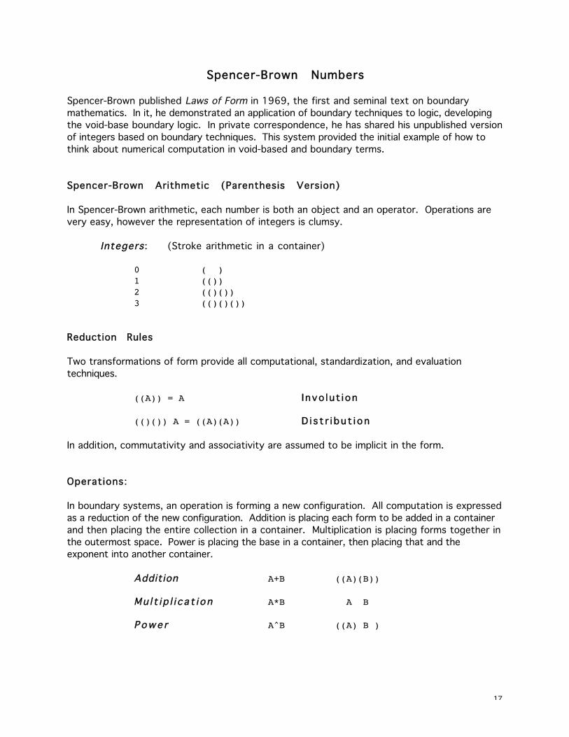
Spencer-Brown Numbers

Spencer-Brown published Laws of Form in 1969, the first and seminal text on boundary

mathematics. In it, he demonstrated an application of boundary techniques to logic, developing

the void-base boundary logic. In private correspondence, he has shared his unpublished version

of integers based on boundary techniques. This system provided the initial example of how to

think about numerical computation in void-based and boundary terms.

Spencer-Brown Arithmetic (Parenthesis Version)

In Spencer-Brown arithmetic, each number is both an object and an operator. Operations are

very easy, however the representation of integers is clumsy.

Integers: (Stroke arithmetic in a container)

0 ( )1 (())2 (()())3 (()()())

Reduction Rules

Two transformations of form provide all computational, standardization, and evaluation

techniques.

((A)) = A I nvo l u t i on

(()()) A = ((A)(A)) D i s t r i bu t i on

In addition, commutativity and associativity are assumed to be implicit in the form.

Operations:

In boundary systems, an operation is forming a new configuration. All computation is expressed

as a reduction of the new configuration. Addition is placing each form to be added in a container

and then placing the entire collection in a container. Multiplication is placing forms together in

the outermost space. Power is placing the base in a container, then placing that and the

exponent into another container.

Addition A+B ((A)(B))

Mu l t i p l i c a t i o n A*B A B

P o w e r A^B ((A) B )

18

The containers themselves do not have an interpretation in conventional numerics. They

maintain structural relations between spaces; the structures do have meaning as both

numerical objects and as operations.

Alternatively, sharing space can be interpreted as addition, while double-bounding becomes

multiplication. Since this is the strategy of both Kauffman numbers and James numbers,

therefore only the above interpretation is presented here.

Confounding Objects and Operations

The form of an integer is also the form of addition. This is characteristic of boundary systems

which confound containment as a function with container as an object. That is:

0 = ( ) = 01 = (()) = +02 = (()()) = 0+03 = (()()()) = 0+0+0

Spencer-Brown integers count the cardinality of nothings added together. An integer is the

cardinality of partitions of an empty set. This is a link between Conway (set) systems and other

boundary systems.

Since we can also interpret a form functionally, a "number" is the cardinality of an application

of the distribution rule.

(( )( )( )) A 3*A implicitly

((A)(A)(A)) A+A+A explicitly

Addition is placing the forms to be added in separate spaces, two levels deep. Multiplication is

placing forms in the same space at the zero, or top, level. The capital letter A means than any

form (not just numbers) can participate in these transformations. The absence of a form, the

void, is excluded from this system.

By suppressing the stability of units ( ), a binary system is created with bases ( ) and (( )).

This system is morphic to propositional logic and finite set theory. The idempotent equation

which converts inters into logic and collections is:

( )( ) = ( ) CALL (idempotency)

Computation

Compound forms are constructed via algebraic substitution. These forms reduce using the two

reduction rules. In essence, the container around a number-object cancels with the void

containers inside a number/operator, producing a new number form through the involution

transform.

19

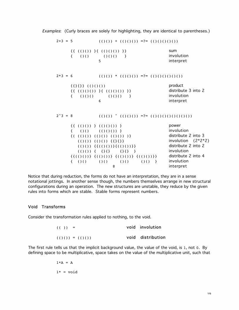
Examples: (Curly braces are solely for highlighting, they are identical to parentheses.)

2+3 = 5 (()()) + (()()()) =?= (()()()()())

{{ (()()) }{ (()()()) }} sum

{ ()() ()()() } involution

5 interpret

2*3 = 6 (()()) * (()()()) =?= (()()()()()())

{{}{}} (()()()) product

{{ (()()()) }{ (()()()) }} distribute 3 into 2

{ ()()() ()()() } involution

6 interpret

2^3 = 8 (()()) ^ (()()()) =?= (()()()()()()()())

{{ (()()) } (()()()) } power

{ ()() (()()()) } involution

{( (()()) (()()) (()()) )} distribute 2 into 3

(()()) (()()) {{}{}} involution (2*2*2)

(()()) {{(()())}{(()())}} distribute 2 into 2

(()()) { {}{} {}{} } involution

{{(()())} {(()())} {(()())} {(()())}} distribute 2 into 4

{ ()() ()() ()() ()() } involution

8 interpret

Notice that during reduction, the forms do not have an interpretation, they are in a sense

notational jottings. In another sense though, the numbers themselves arrange in new structural

configurations during an operation. The new structures are unstable, they reduce by the given

rules into forms which are stable. Stable forms represent numbers.

Void Transforms

Consider the transformation rules applied to nothing, to the void.

(( )) = void involution

(()()) = (()()) void distribution

The first rule tells us that the implicit background value, the value of the void, is 1, not 0. By

defining space to be multiplicative, space takes on the value of the multiplicative unit, such that

1*A = A

1* = void

20

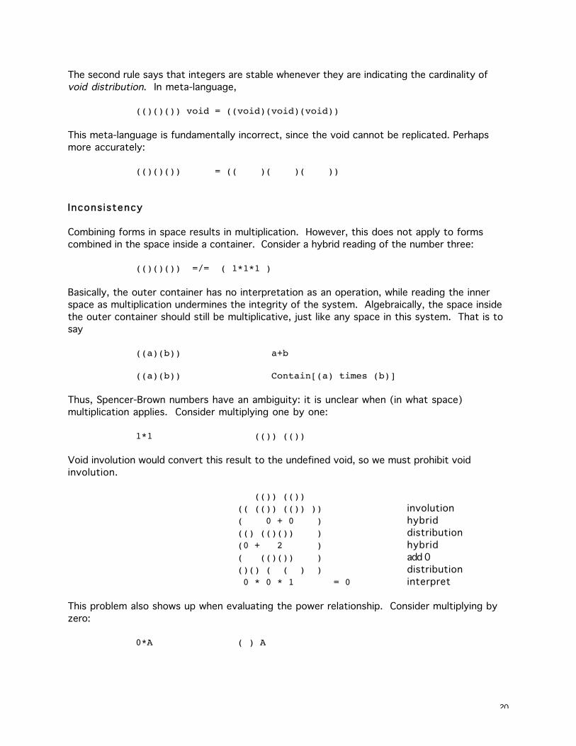
The second rule says that integers are stable whenever they are indicating the cardinality of

void distribution. In meta-language,

(()()()) void = ((void)(void)(void))

This meta-language is fundamentally incorrect, since the void cannot be replicated. Perhaps

more accurately:

(()()()) = (( )( )( ))

Inconsistency

Combining forms in space results in multiplication. However, this does not apply to forms

combined in the space inside a container. Consider a hybrid reading of the number three:

(()()()) =/= ( 1*1*1 )

Basically, the outer container has no interpretation as an operation, while reading the inner

space as multiplication undermines the integrity of the system. Algebraically, the space inside

the outer container should still be multiplicative, just like any space in this system. That is to

say

((a)(b)) a+b

((a)(b)) Contain[(a) times (b)]

Thus, Spencer-Brown numbers have an ambiguity: it is unclear when (in what space)

multiplication applies. Consider multiplying one by one:

1*1 (()) (())

Void involution would convert this result to the undefined void, so we must prohibit void

involution.

(()) (())(( (()) (()) )) involution

( 0 + 0 ) hybrid

(() (()()) ) distribution

(0 + 2 ) hybrid

( (()()) ) add 0

()() ( ( ) ) distribution

0 * 0 * 1 = 0 interpret

This problem also shows up when evaluating the power relationship. Consider multiplying by

zero:

0*A ( ) A

21

We need a new rule to be able to reduce this to 0. Spencer-Brown suggests that the

configuration is an instruction to multiply, and multiplication takes place by distribution.

Therefore, A must distribute into ( ). Since there is nothing to distribute into, the A is

absorbed by the void.

( ) A = ( )

It is generally agreed that this is not a strong argument, although it is very similar to Conway's

handling of void partitions when testing for a number. Still the problem recurs for the

representation of powers.

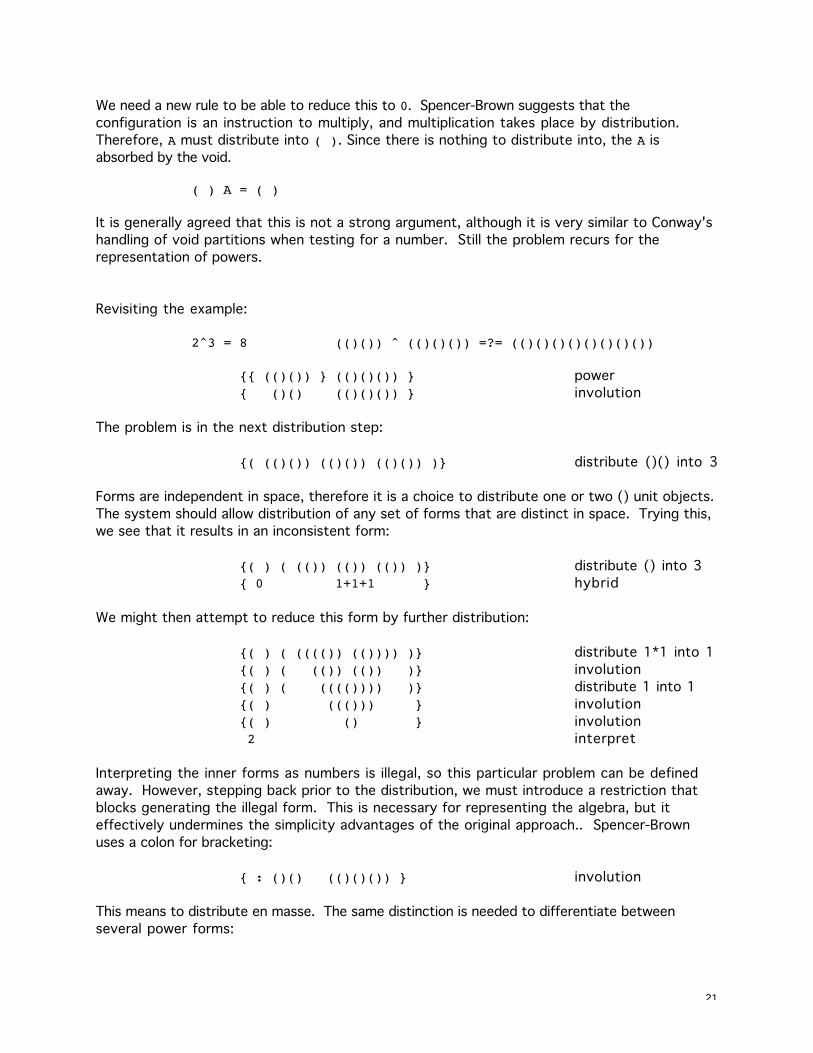
Revisiting the example:

2^3 = 8 (()()) ^ (()()()) =?= (()()()()()()()())

{{ (()()) } (()()()) } power

{ ()() (()()()) } involution

The problem is in the next distribution step:

{( (()()) (()()) (()()) )} distribute ()() into 3

Forms are independent in space, therefore it is a choice to distribute one or two () unit objects.

The system should allow distribution of any set of forms that are distinct in space. Trying this,

we see that it results in an inconsistent form:

{( ) ( (()) (()) (()) )} distribute () into 3

{ 0 1+1+1 } hybrid

We might then attempt to reduce this form by further distribution:

{( ) ( (((()) (()))) )} distribute 1*1 into 1

{( ) ( (()) (()) )} involution

{( ) ( (((()))) )} distribute 1 into 1

{( ) ((())) } involution

{( ) () } involution

2 interpret

Interpreting the inner forms as numbers is illegal, so this particular problem can be defined

away. However, stepping back prior to the distribution, we must introduce a restriction that

blocks generating the illegal form. This is necessary for representing the algebra, but it

effectively undermines the simplicity advantages of the original approach.. Spencer-Brown

uses a colon for bracketing:

{ : ()() (()()()) } involution

This means to distribute en masse. The same distinction is needed to differentiate between

several power forms:

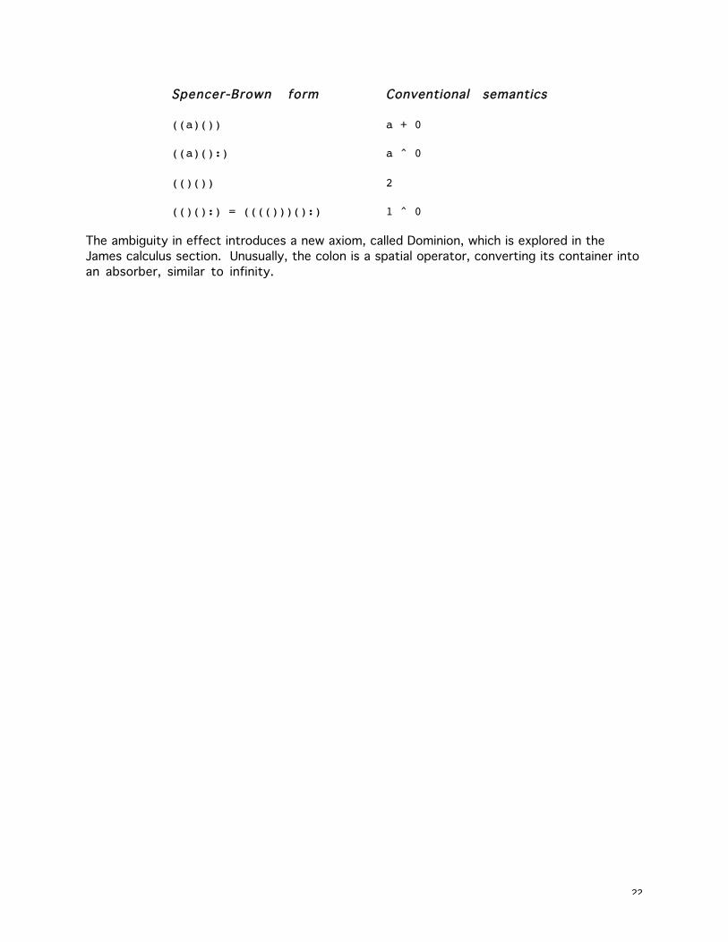
22

Spencer-Brown form Conventional semantics

((a)()) a + 0

((a)():) a ^ 0

(()()) 2

(()():) = (((()))():) 1 ^ 0

The ambiguity in effect introduces a new axiom, called Dominion, which is explored in the

James calculus section. Unusually, the colon is a spatial operator, converting its container into

an absorber, similar to infinity.

23

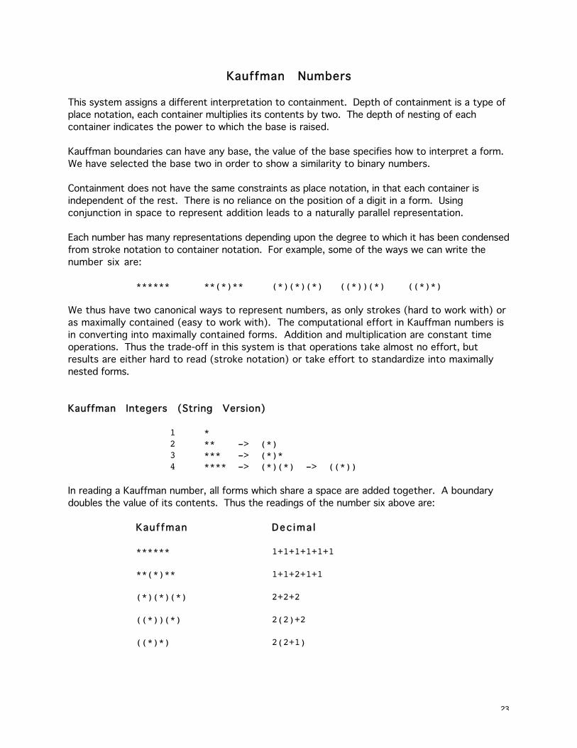
Kauffman Numbers

This system assigns a different interpretation to containment. Depth of containment is a type of

place notation, each container multiplies its contents by two. The depth of nesting of each

container indicates the power to which the base is raised.

Kauffman boundaries can have any base, the value of the base specifies how to interpret a form.

We have selected the base two in order to show a similarity to binary numbers.

Containment does not have the same constraints as place notation, in that each container is

independent of the rest. There is no reliance on the position of a digit in a form. Using

conjunction in space to represent addition leads to a naturally parallel representation.

Each number has many representations depending upon the degree to which it has been condensed

from stroke notation to container notation. For example, some of the ways we can write the

number six are:

****** **(*)** (*)(*)(*) ((*))(*) ((*)*)

We thus have two canonical ways to represent numbers, as only strokes (hard to work with) or

as maximally contained (easy to work with). The computational effort in Kauffman numbers is

in converting into maximally contained forms. Addition and multiplication are constant time

operations. Thus the trade-off in this system is that operations take almost no effort, but

results are either hard to read (stroke notation) or take effort to standardize into maximally

nested forms.

Kauffman Integers (String Version)

1 *2 ** -> (*)3 *** -> (*)*4 **** -> (*)(*) -> ((*))

In reading a Kauffman number, all forms which share a space are added together. A boundary

doubles the value of its contents. Thus the readings of the number six above are:

Kauffman Dec ima l

****** 1+1+1+1+1+1

**(*)** 1+1+2+1+1

(*)(*)(*) 2+2+2

((*))(*) 2(2)+2

((*)*) 2(2+1)

24

Each star is a unit, each container delineates an order of magnitude in the chosen base. The

notation is not in a particular base, since added contents may sun to more than that base.

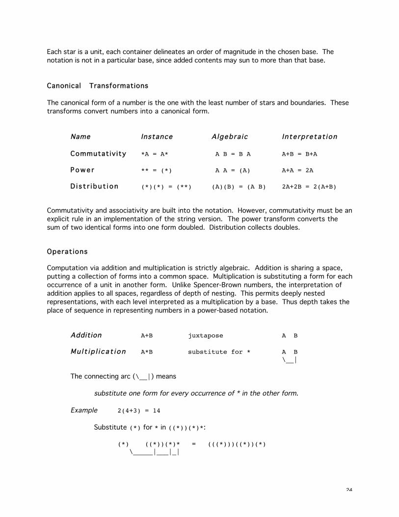
Canonical Transformations

The canonical form of a number is the one with the least number of stars and boundaries. These

transforms convert numbers into a canonical form.

Name Instance Algebra ic Interpretat ion

Commutat iv ity *A = A* A B = B A A+B = B+A

P o w e r ** = (*) A A = (A) A+A = 2A

D i s t r i bu t i on (*)(*) = (**) (A)(B) = (A B) 2A+2B = 2(A+B)

Commutativity and associativity are built into the notation. However, commutativity must be an

explicit rule in an implementation of the string version. The power transform converts the

sum of two identical forms into one form doubled. Distribution collects doubles.

Operat ions

Computation via addition and multiplication is strictly algebraic. Addition is sharing a space,

putting a collection of forms into a common space. Multiplication is substituting a form for each

occurrence of a unit in another form. Unlike Spencer-Brown numbers, the interpretation of

addition applies to all spaces, regardless of depth of nesting. This permits deeply nested

representations, with each level interpreted as a multiplication by a base. Thus depth takes the

place of sequence in representing numbers in a power-based notation.

Addition A+B juxtapose A B

Mu l t i p l i c a t i o n A*B substitute for * A B\__|

The connecting arc (\__|) means

substitute one form for every occurrence of * in the other form.

Example 2(4+3) = 14

Substitute (*) for * in ((*))(*)*:

(*) ((*))(*)* = (((*)))((*))(*) \_____|___|_|

25

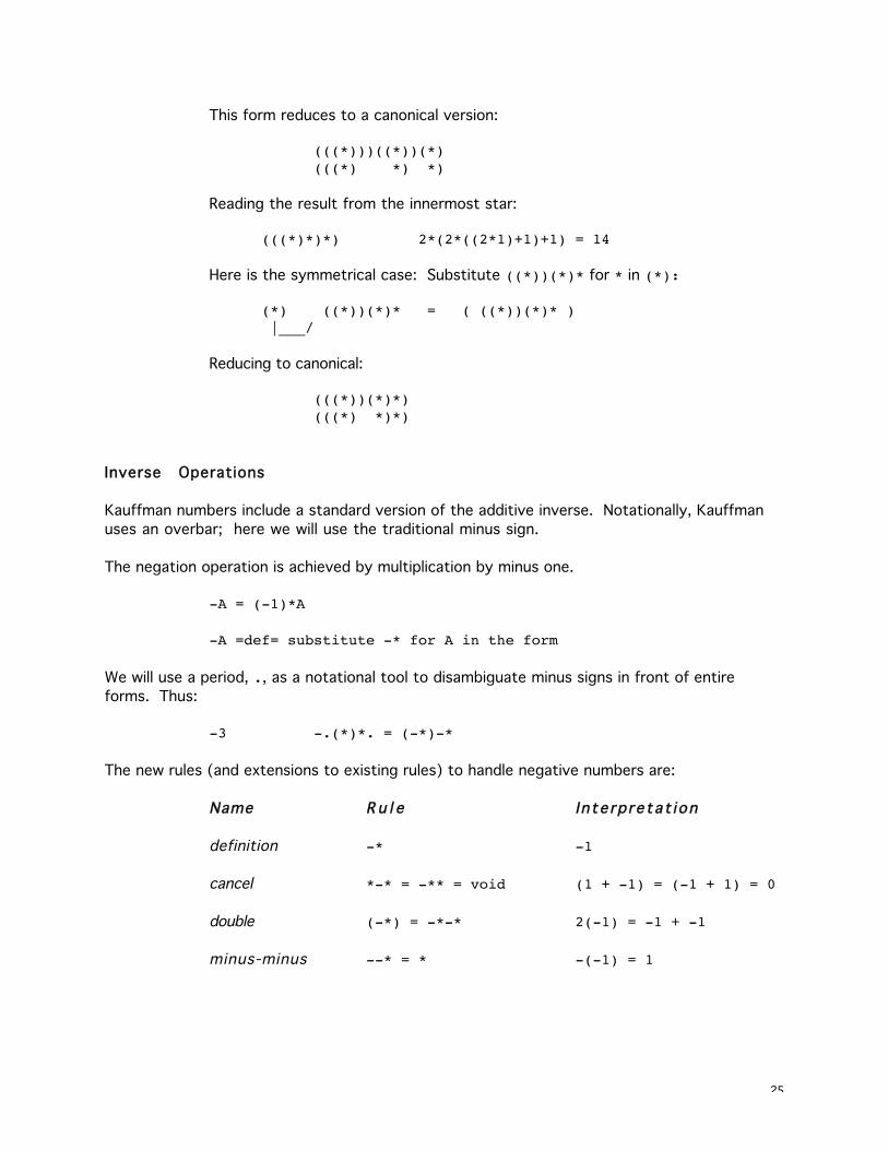
This form reduces to a canonical version:

(((*)))((*))(*)(((*) *) *)

Reading the result from the innermost star:

(((*)*)*) 2*(2*((2*1)+1)+1) = 14

Here is the symmetrical case: Substitute ((*))(*)* for * in (*):

(*) ((*))(*)* = ( ((*))(*)* ) |___/

Reducing to canonical:

(((*))(*)*)(((*) *)*)

Inverse Operations

Kauffman numbers include a standard version of the additive inverse. Notationally, Kauffman

uses an overbar; here we will use the traditional minus sign.

The negation operation is achieved by multiplication by minus one.

-A = (-1)*A

-A =def= substitute -* for A in the form

We will use a period, ., as a notational tool to disambiguate minus signs in front of entire

forms. Thus:

-3 -.(*)*. = (-*)-*

The new rules (and extensions to existing rules) to handle negative numbers are:

Name R u l e Interpretat ion

definition -* -1

cancel *-* = -** = void (1 + -1) = (-1 + 1) = 0

double (-*) = -*-* 2(-1) = -1 + -1

minus-minus --* = * -(-1) = 1

26

These two rules permit negative numbers to migrate across doubling boundaries:

compensate (A)* = (A *)-* 2A + 1 = 2(A+1) - 1

subtract (A)-* = (A -*)* 2A - 1 = 2(A-1) + 1

Division is handled by a new type of boundary, the inverse of the doubling boundary.

definition [A] A/2

divide ([A]) = [(A)] = A 2(A/2) = (2A)/2 = A

We will not cover division here. An example of subtraction follows:

6 - 2

((*)*)-(*) transcribe

((*)*)(-*) negation

((*)* -*) distribution

((*) ) cancel

4 interpret

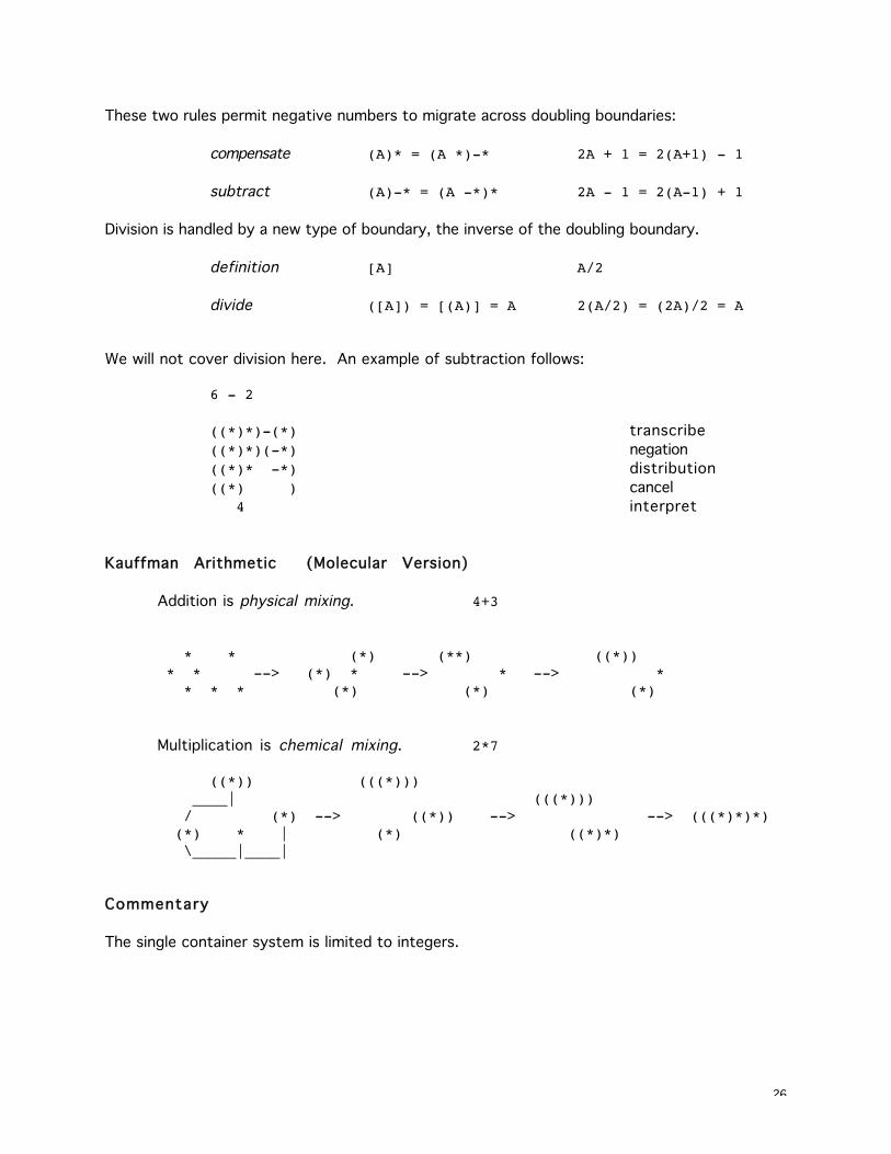
Kauffman Arithmetic (Molecular Version)

Addition is physical mixing. 4+3

* * (*) (**) ((*)) * * --> (*) * --> * --> * * * * (*) (*) (*)

Multiplication is chemical mixing. 2*7

((*)) (((*))) ____| (((*))) / (*) --> ((*)) --> --> (((*)*)*) (*) * | (*) ((*)*)

\_____|____|

Commentary

The single container system is limited to integers.

27

Bricken Graph-numbers

These numbers are a parallel implementation of Kauffman numbers, with some extensions.

The following presentation is in a different style than those in other sections of this document.

BOUNDARY NUMBERS specify a formal redefinition of the concept of number. Rather than being

inert objects that are operated upon, boundary numbers are active objects that computethemselves. This is a fundamental refocusing of the concepts of object and operator. Rather

than having easily stated and relatively useless numerical objects coupled with computation

intensive operators, the boundary model is:

ACTIVE OBJECTS that dynamically compute their value

coupled with easily stated and relatively inert OPERATORS.

Thus, the computational effort is in finding out the value of a boundary representation of a

number. Operating on boundary numbers is a trivial process; operations are independent of themagnitude of the numbers being manipulated.

The computational trade-off, then, is in determining the value of a result. The READING process

is strongly parallel and more efficient than traditional computation. (Reading a value is log(n),

where n is the number of bits in the binary representation of the result.) And reading is

required only once, when the result of any combination of operations is desired.

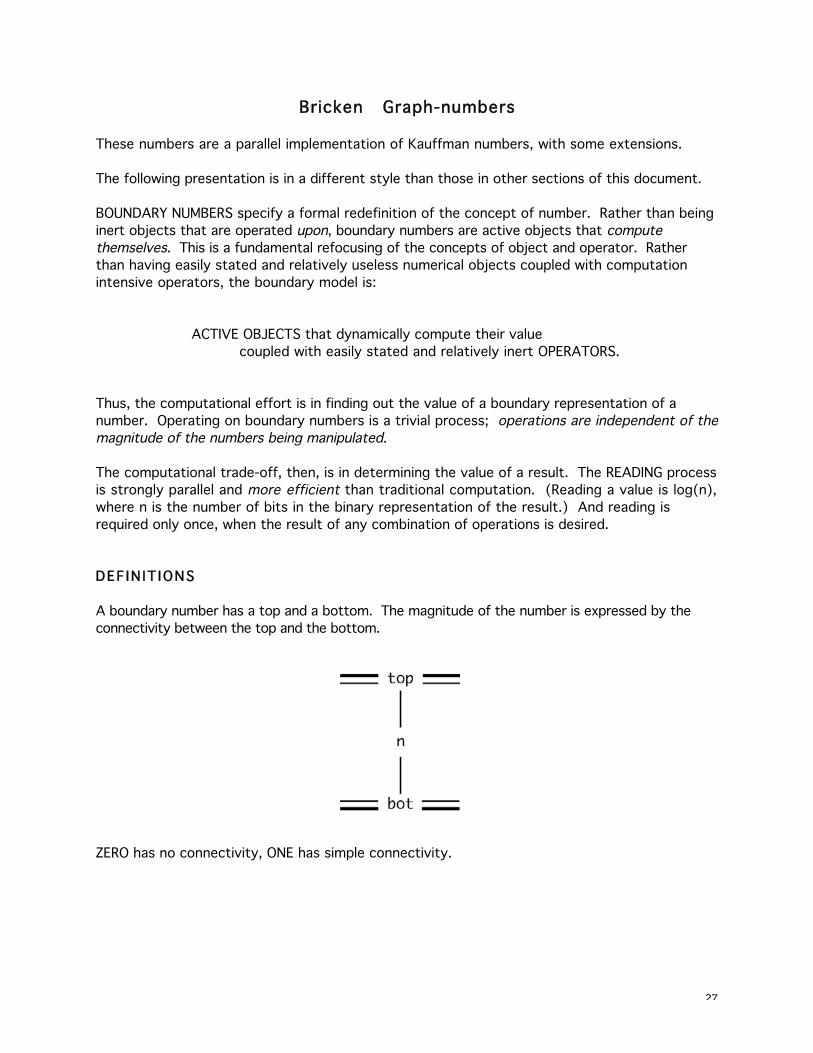
DEF IN IT IONS

A boundary number has a top and a bottom. The magnitude of the number is expressed by the

connectivity between the top and the bottom.

ZERO has no connectivity, ONE has simple connectivity.

28

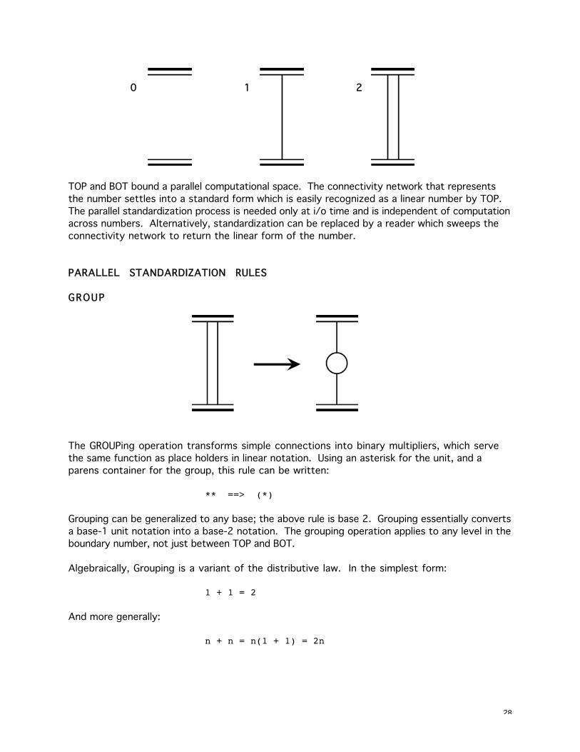
0 11 22

TOP and BOT bound a parallel computational space. The connectivity network that represents

the number settles into a standard form which is easily recognized as a linear number by TOP.

The parallel standardization process is needed only at i/o time and is independent of computation

across numbers. Alternatively, standardization can be replaced by a reader which sweeps the

connectivity network to return the linear form of the number.

PARALLEL STANDARDIZATION RULES

GROUP

The GROUPing operation transforms simple connections into binary multipliers, which serve

the same function as place holders in linear notation. Using an asterisk for the unit, and a

parens container for the group, this rule can be written:

** ==> (*)

Grouping can be generalized to any base; the above rule is base 2. Grouping essentially converts

a base-1 unit notation into a base-2 notation. The grouping operation applies to any level in the

boundary number, not just between TOP and BOT.

Algebraically, Grouping is a variant of the distributive law. In the simplest form:

1 + 1 = 2

And more generally:

n + n = n(1 + 1) = 2n

29

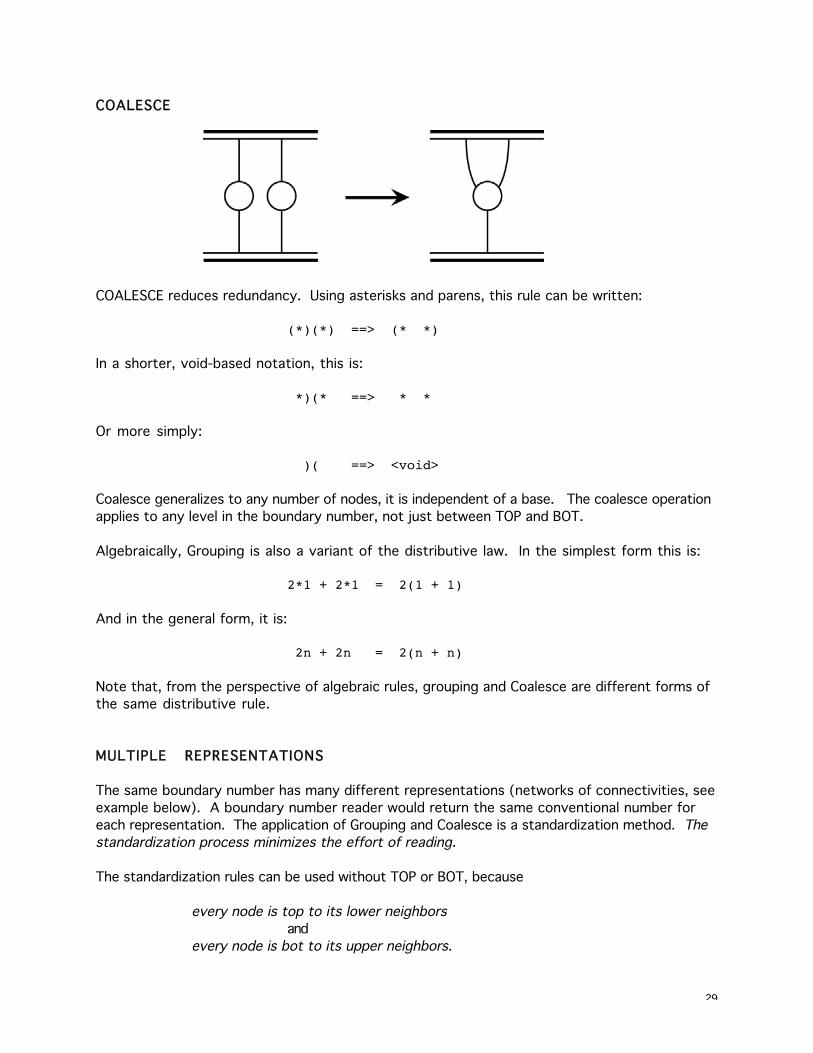
COALESCE

COALESCE reduces redundancy. Using asterisks and parens, this rule can be written:

(*)(*) ==> (* *)

In a shorter, void-based notation, this is:

*)(* ==> * *

Or more simply:

)( ==> <void>

Coalesce generalizes to any number of nodes, it is independent of a base. The coalesce operation

applies to any level in the boundary number, not just between TOP and BOT.

Algebraically, Grouping is also a variant of the distributive law. In the simplest form this is:

2*1 + 2*1 = 2(1 + 1)

And in the general form, it is:

2n + 2n = 2(n + n)

Note that, from the perspective of algebraic rules, grouping and Coalesce are different forms of

the same distributive rule.

MULTIPLE REPRESENTATIONS

The same boundary number has many different representations (networks of connectivities, see

example below). A boundary number reader would return the same conventional number for

each representation. The application of Grouping and Coalesce is a standardization method. Thestandardization process minimizes the effort of reading.

The standardization rules can be used without TOP or BOT, because

every node is top to its lower neighborsand

every node is bot to its upper neighbors.

30

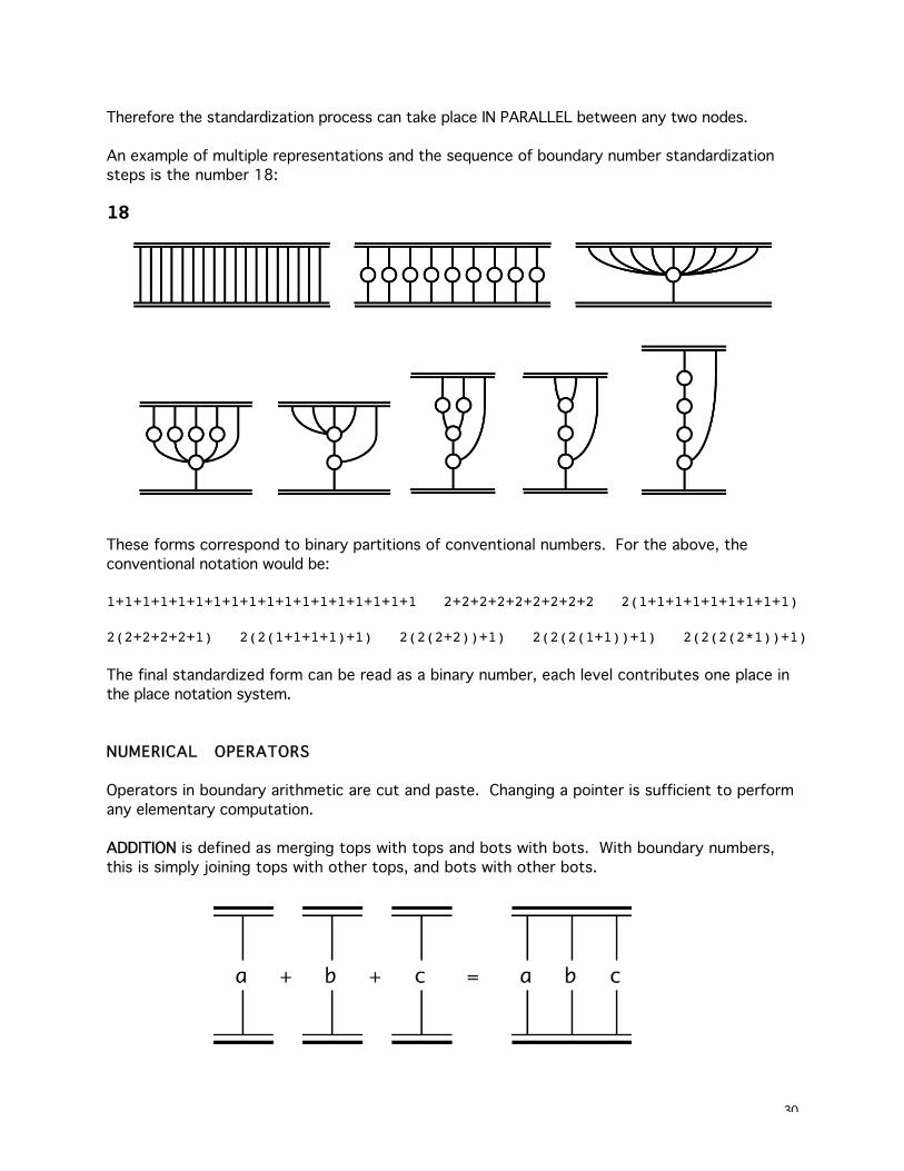
Therefore the standardization process can take place IN PARALLEL between any two nodes.

An example of multiple representations and the sequence of boundary number standardization

steps is the number 18:

18

These forms correspond to binary partitions of conventional numbers. For the above, the

conventional notation would be:

1+1+1+1+1+1+1+1+1+1+1+1+1+1+1+1+1+1 2+2+2+2+2+2+2+2+2 2(1+1+1+1+1+1+1+1+1)

2(2+2+2+2+1) 2(2(1+1+1+1)+1) 2(2(2+2))+1) 2(2(2(1+1))+1) 2(2(2(2*1))+1)

The final standardized form can be read as a binary number, each level contributes one place in

the place notation system.

NUMERICAL OPERATORS

Operators in boundary arithmetic are cut and paste. Changing a pointer is sufficient to perform

any elementary computation.

ADDITION is defined as merging tops with tops and bots with bots. With boundary numbers,

this is simply joining tops with other tops, and bots with other bots.

31

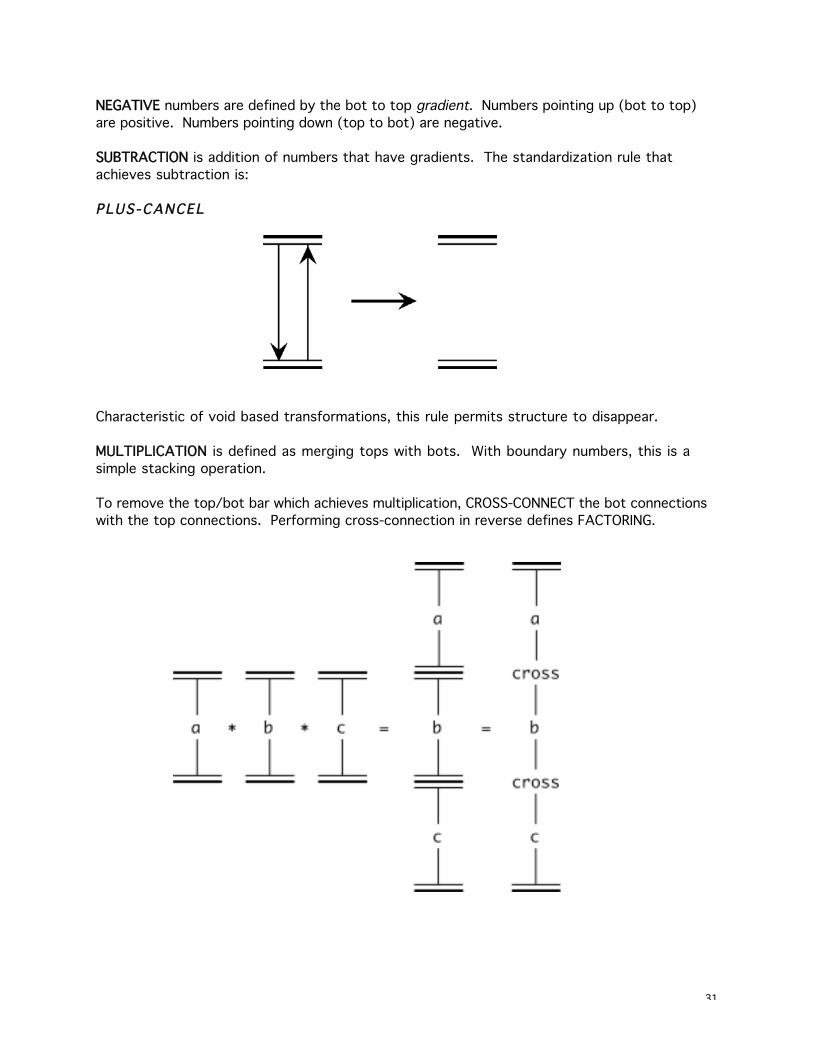
NEGATIVE numbers are defined by the bot to top gradient. Numbers pointing up (bot to top)

are positive. Numbers pointing down (top to bot) are negative.

SUBTRACTION is addition of numbers that have gradients. The standardization rule that

achieves subtraction is:

PLUS-CANCEL

Characteristic of void based transformations, this rule permits structure to disappear.

MULTIPLICATION is defined as merging tops with bots. With boundary numbers, this is a

simple stacking operation.

To remove the top/bot bar which achieves multiplication, CROSS-CONNECT the bot connections

with the top connections. Performing cross-connection in reverse defines FACTORING.

32

CROSS-CONNECT

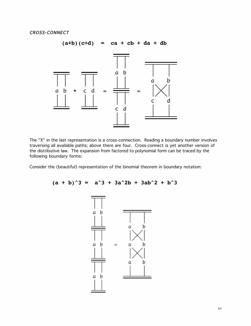
(a+b)(c+d) = ca + cb + da + db

The "X" in the last representation is a cross-connection. Reading a boundary number involves

traversing all available paths; above there are four. Cross-connect is yet another version of

the distributive law. The expansion from factored to polynomial form can be traced by the

following boundary forms:

Consider the (beautiful) representation of the binomial theorem in boundary notation:

(a + b)^3 = a^3 + 3a^2b + 3ab^2 + b^3

33

The right-hand-side represents eight paths from bot to top. One path passes through three aforms; three paths pass through two a forms and one b form. Similarly, three paths pas

through two b forms and one a form, and one path threads through all three b forms.

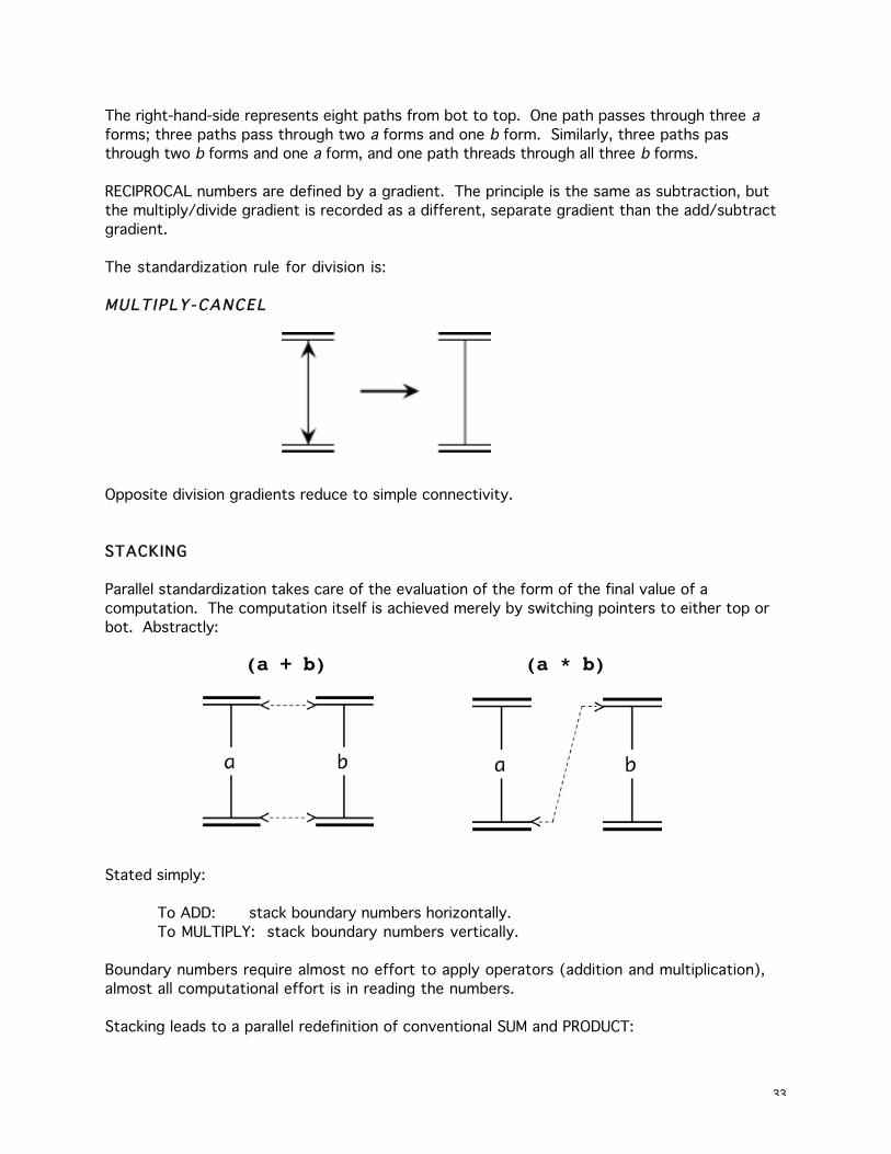
RECIPROCAL numbers are defined by a gradient. The principle is the same as subtraction, but

the multiply/divide gradient is recorded as a different, separate gradient than the add/subtract

gradient.

The standardization rule for division is:

MULT IPLY -CANCEL

Opposite division gradients reduce to simple connectivity.

STACKING

Parallel standardization takes care of the evaluation of the form of the final value of a

computation. The computation itself is achieved merely by switching pointers to either top or

bot. Abstractly:

(a + b) (a * b)

Stated simply:

To ADD: stack boundary numbers horizontally.

To MULTIPLY: stack boundary numbers vertically.

Boundary numbers require almost no effort to apply operators (addition and multiplication),

almost all computational effort is in reading the numbers.

Stacking leads to a parallel redefinition of conventional SUM and PRODUCT:

34

SUM[1..n] PRODUCT[1..n]

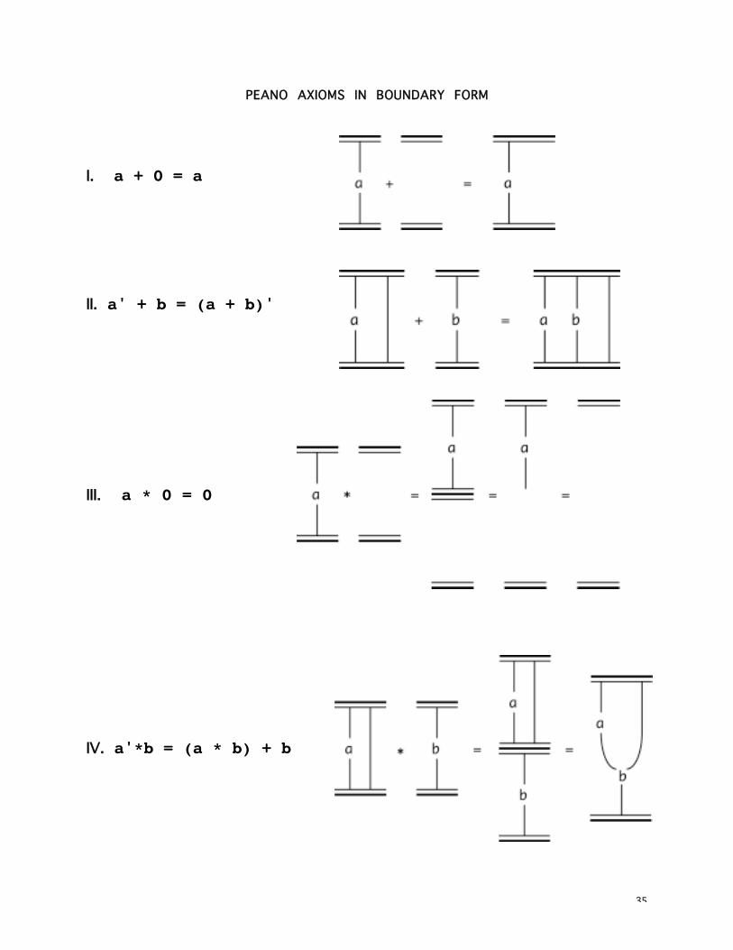
PEANO AXIOMS FOR ARITHMETIC

The four Peano axioms for the construction of arithmetic are shown in boundary notation at the

end of this paper. Here are some observations about their spatial form:

1. Induction is not needed as a reasoning axiom. Instead it is subsumed by the parallel process

of standardization. For boundary variables to standardize, connectivities that represent

magnitude must be decomposed pictorially (by running the standardization rules backwards).

The decomposition steps achieve induction, but are more efficient.

2. The concept of a successor function is not really needed either. The cut and paste definitions

of boundary + and * are a sufficient axiomatization of the operators. For the addition operation,

the successor function is confounded with parallel standardization of representations in the

same space. In multiplication, the successor is confounded with cross-connection of stacked

representations.

3. The zero axioms are quite unnecessary. The marvelous characteristic of void based

representation is that the SYMBOL OF NOTHING is replaced by a LITERAL NOTHING. During

computation, the halting condition is nonexistence of connectivity rather than the identification

of a special token for bottom (i.e. "0").

4. The final rewrite in Axioms III and IV illustrates the similarity of boundary notation to the

linear notation for Peano's definitions. They are not necessary within the network connectivity

formalism.

5. The general rule of parallel boundary operations is: recording the problem is sufficient togenerate the answer. All effort is in reading the result, and this need be done once at the exit to

computation.

35

PEANO AXIOMS IN BOUNDARY FORM

I. a + 0 = a

II. a' + b = (a + b)'

III. a * 0 = 0

IV. a'*b = (a * b) + b

36

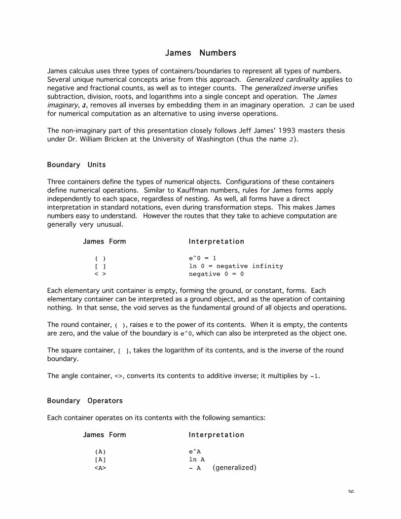
James Numbers

James calculus uses three types of containers/boundaries to represent all types of numbers.

Several unique numerical concepts arise from this approach. Generalized cardinality applies to

negative and fractional counts, as well as to integer counts. The generalized inverse unifies

subtraction, division, roots, and logarithms into a single concept and operation. The Jamesimaginary, J, removes all inverses by embedding them in an imaginary operation. J can be used

for numerical computation as an alternative to using inverse operations.

The non-imaginary part of this presentation closely follows Jeff James' 1993 masters thesis

under Dr. William Bricken at the University of Washington (thus the name J).

Boundary Units

Three containers define the types of numerical objects. Configurations of these containers

define numerical operations. Similar to Kauffman numbers, rules for James forms apply

independently to each space, regardless of nesting. As well, all forms have a direct

interpretation in standard notations, even during transformation steps. This makes James

numbers easy to understand. However the routes that they take to achieve computation are

generally very unusual.

JJames Form Interpretat ion

( ) e^0 = 1[ ] ln 0 = negative infinity< > negative 0 = 0

Each elementary unit container is empty, forming the ground, or constant, forms. Each

elementary container can be interpreted as a ground object, and as the operation of containing

nothing. In that sense, the void serves as the fundamental ground of all objects and operations.

The round container, ( ), raises e to the power of its contents. When it is empty, the contents

are zero, and the value of the boundary is e^0, which can also be interpreted as the object one.

The square container, [ ], takes the logarithm of its contents, and is the inverse of the round

boundary.

The angle container, <>, converts its contents to additive inverse; it multiplies by -1.

Boundary Operators

Each container operates on its contents with the following semantics:

JJames Form Interpretat ion

(A) e^A[A] ln A<A> - A (generalized)

37

The exponent and logarithm transforms can be in an arbitrary base. Let the base be represented

by #. Then the following remains true:

( ) #^0 = 1[ ] log# 0 = negative infinity

(A) #^A[A] log# A

The base of natural logarithms, e, is most convenient as a specific choice, since many

irrationals are defined in terms of e.

Integers

James integers are expressed in stroke notation. There is no provision for a power-oriented

notation for integers, however the calculus itself uses power transformations extensively.

0 void1 ( )2 ( )( )3 ( )( )( )...

Varieties of numbers occur through configurations of the three containers, with empty

containers forming a computational ground. The calculus emphasizes algebraic forms, and is

clumsy for arithmetic evaluation.

Since stroke representation is rather clumsy, we will use decimal numbers to abbreviate

stroke numbers throughout this section.

Algebraic Operations

Addition is sharing space. All forms inside the same container, that is, all forms sharing a

space, are joined by implicit addition. Multiplication and power are specific configurations of

( ) and [ ] containers, both of which keep track of the appropriate exponential or logarithmic

space. Multiplication is adding logarithms then converting back the non-logarithmic space.

Power is adding the loglog form of the base to the log of the exponent.

Addition A+B A B

Mu l t i p l i c a t i o n A*B ( [A] [B])

P o w e r A^B (([[A]][B]))

The round and square boundaries can be read as exponents and natural logs, providing James

forms with a direct interpretation:

38

Operat ion James Form Interpretat ion

A+B A B A + B

A*B ([A][B]) e^(ln A + ln B) =e^ln A * e^ln BA * B

A^B (([[A]][B])) e^(e^(lnln A + ln B)) =e^(e^lnln A * e^ln B)e^((ln A) * B)e^(ln A^B)A ^ B

It is fair to say that round and square boundaries are simply a convenient way write complex

exponents, since they introduce no new transformation rules. Similar to Spencer-Brown

numbers, James notation could use a single container by indexing the depth of containments:

even is exponent ( ), odd is logarithm [ ]. Similar to Kauffman numbers, a fourth boundary

type could be used for a depth-oriented positional notation.

Inverse Operations

Subtraction is sharing a space with an additive inverse form, . Division is sharing deeper

space with a multiplicative inverse form, <[B]>. Taking a root is sharing an even deeper space

with the multiplicative inverse form.

Subtract ion A-B A 

D i v i s i o n A/B ( [A] <[B]>)

Root A^(1/B) (([[A]]<[B]>))

The angle container, <>, serves as the inversion concept for all inverse operations. The

operations are distinguished by which forms are contained in angle boundaries, and by the depth

of nesting of exp-log transforms.

Reduction Rules (Axiomatic basis)

Computation is achieved through application of three reduction rules:

([A]) = [(A)] = A I nvo l u t i on

(A [B]) (A [C]) = (A [B C]) D i s t r i bu t i on

A <A> = void I n v e r s i o n

The distribution rule in standard notation would read:

39

e^(A+ln B) + e^(A+ln C) = e^(A+ln(B+C))

Proof:

e^(A+ln B) = (eÂ)*(e^ln B) = B*(eÂ)e^(A+ln C) = (eÂ)*(e^ln C) = C*(eÂ)

B*(eÂ) + C*(eÂ) = (eÂ)(B+C)= (eÂ)(e^ln(B+C))= e^(A + ln(B+C))

Alternatively, we could convert the distributive rule into a multiplicative rather than an

additive form:

( A [B]) ( A [C]) = ( A [B C]) additive

([A][B]) ([A][C]) = ([A][B C]) multiplicative

which reads more conventionally as:

(A*B)+(A*C) = A*(B+C)

and more unconventionally as exponents and logs:

e^(ln A + ln B) + e^(ln A + ln C) = e^(ln A + ln(B+C))

Note that the multiplicative representation uses [A] rather than A. This is not a significant

difference, since any form can be bounded by [ ] due to involution:

A = [(A)]

Algebraic Proof

James calculus is an algebraic, equational system. The primary transformations are

substitution and replacement of equals for equals. Proof consists of a series of transformations

from one form into another.

The standard substitution strategies are all available in the boundary calculus. Given an

equation A=?=B, the two forms can be demonstrated to be equal by:

Convert one form into the other form.

Convert both forms into the same third form

Standardize the equation to a void-equivalent and reduce to void.

To standardize to a void-equivalent, we place all terms on one side of the equation, leaving the

other side void. Unlike conventional algebra, there is only one operation, Inversion, to move all

terms to one side of an equation:

40

A = B

A = B = void

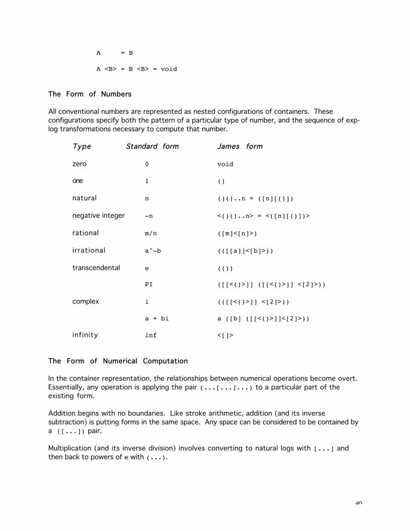
The Form of Numbers

All conventional numbers are represented as nested configurations of containers. These

configurations specify both the pattern of a particular type of number, and the sequence of exp-

log transformations necessary to compute that number.

Type Standard form James form

zero 0 void

one 1 ()

natural n ()()..n = ([n][()])

negative integer -n <()()..n> = <([n][()])>

rational m/n ([m]<[n]>)

irrational a^-b (([[a]]<[b]>))

transcendental e (())

PI ([[<()>]] ([[<()>]] <[2]>))

complex i (([[<()>]] <[2]>))

a + bi a ([b] ([[<()>]]<[2]>))

infinity inf <[]>

The Form of Numerical Computation

In the container representation, the relationships between numerical operations become overt.

Essentially, any operation is applying the pair (...[...]...) to a particular part of the

existing form.

Addition begins with no boundaries. Like stroke arithmetic, addition (and its inverse

subtraction) is putting forms in the same space. Any space can be considered to be contained by

a ([...]) pair.

Multiplication (and its inverse division) involves converting to natural logs with [...] and

then back to powers of e with (...).

41

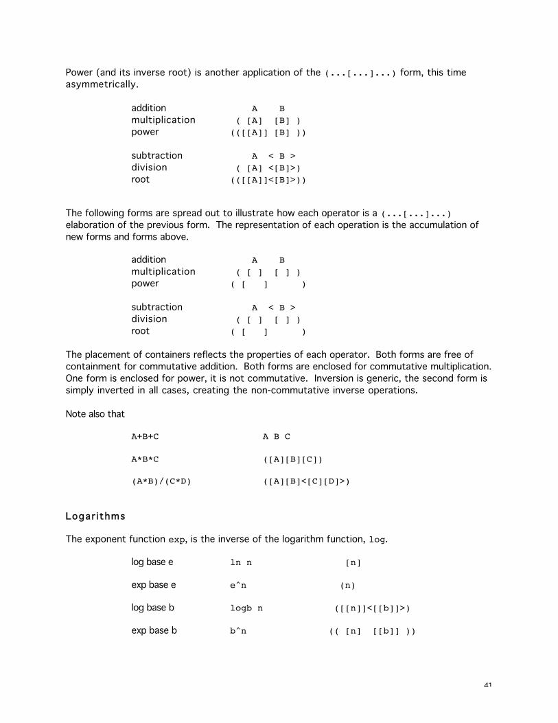
Power (and its inverse root) is another application of the (...[...]...) form, this time

asymmetrically.

addition A Bmultiplication ( [A] [B] )power (([[A]] [B] ))

subtraction A division ( [A] <[B]>)root (([[A]]<[B]>))

The following forms are spread out to illustrate how each operator is a (...[...]...)elaboration of the previous form. The representation of each operation is the accumulation of

new forms and forms above.

addition A Bmultiplication ( [ ] [ ] )power ( [ ] )

subtraction A division ( [ ] [ ] )root ( [ ] )

The placement of containers reflects the properties of each operator. Both forms are free of

containment for commutative addition. Both forms are enclosed for commutative multiplication.

One form is enclosed for power, it is not commutative. Inversion is generic, the second form is

simply inverted in all cases, creating the non-commutative inverse operations.

Note also that

A+B+C A B C

A*B*C ([A][B][C])

(A*B)/(C*D) ([A][B]<[C][D]>)

Logar i thms

The exponent function exp, is the inverse of the logarithm function, log.

log base e ln n [n]

exp base e e^n (n)

log base b logb n ([[n]]<[[b]]>)

exp base b b^n (( [n] [[b]] ))

42

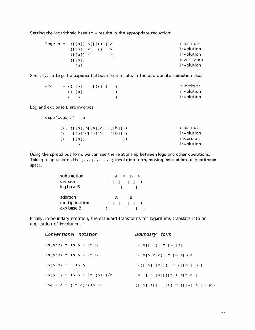
Setting the logarithmic base to e results in the appropriate reduction:

loge n = ([[n]] <[[(())]]>) substitute

([[n]] <[ () ]>) involution

([[n]] < >) involution

([[n]] ) invert zero

[n] involution

Similarly, setting the exponential base to e results in the appropriate reduction also.

e^n = (( [n] [[(())]] )) substitute

(( [n] )) involution

( n ) involution

Log and exp base b are inverses:

expb[logb n] = n

(([ ([[n]]<[[b]]>) ][[b]])) substitute

(( [[n]]<[[b]]> [[b]])) involution

(( [[n]] )) inversion

n involution

Using the spread out form, we can see the relationship between logs and other operations.

Taking a log violates the (...[...]...) involution form, moving instead into a logarithmic

space.

subtraction A division ( [ ] [ ] )log base B [ ] [ ]

addition A Bmultiplication ( [ ] [ ] )exp base B ( [ ] )

Finally, in boundary notation, the standard transforms for logarithms translate into an

application of Involution.

Conventional notation Boundary form

ln(A*B) = ln A + ln B [([A][B])] = [A][B]

ln(A/B) = ln A - ln B [([A]<[B]>)] = [A]<[B]>

ln(A^B) = B ln A [(([[A]][B]))] = ([[A]][B])

ln(n+1) = ln n + ln (n+1)/n [n 1] = [n][([n 1]<[n]>)]

log10 A = (ln A)/(ln 10) ([[A]]<[[10]]>) = ([[A]]<[[10]>)

43

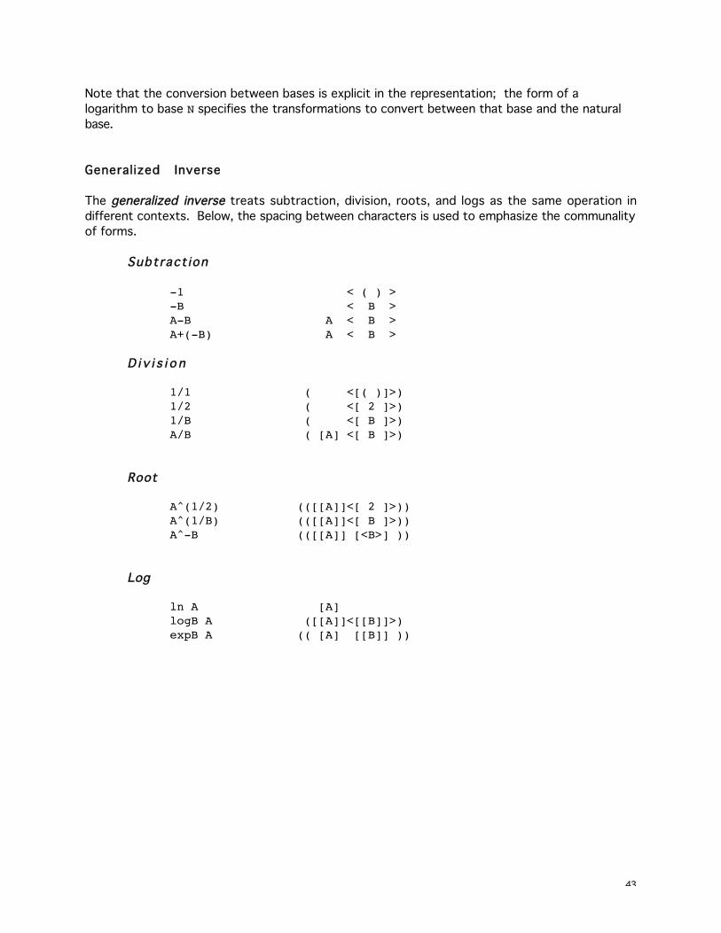
Note that the conversion between bases is explicit in the representation; the form of a

logarithm to base N specifies the transformations to convert between that base and the natural

base.

Generalized Inverse

The generalized inverse treats subtraction, division, roots, and logs as the same operation in

different contexts. Below, the spacing between characters is used to emphasize the communality

of forms.

Subtract ion

-1 < ( ) >-B A-B A A+(-B) A 

D i v i s i o n

1/1 ( <[( )]>)1/2 ( <[ 2 ]>)1/B ( <[ B ]>)A/B ( [A] <[ B ]>)

Root

A^(1/2) (([[A]]<[ 2 ]>))A^(1/B) (([[A]]<[ B ]>))A^-B (([[A]] [] ))

Log

ln A [A]logB A ([[A]]<[[B]]>)expB A (( [A] [[B]] ))

44

Domin ion

An empty square container, [], represents the logarithm of 0, which is negative infinity. The

square basis provides a natural representation of infinity which can be used in the course of

computation. The behavior of infinity is specified by the following theorems.

Name F o r m Interpretat ion

Domin ion A [ ] = [ ] -inf + A = -inf

Negative infinity absorbs all forms sharing its space. A variant of dominion converts the

negative infinity to a void:

(A [ ] ) = void e^(A + -inf) = 0

Positive infinity is the inversion of negative infinity:

<[]> = inf

Positive infinity also absorbs all forms with its space, except for two (negative infinity and the

imaginary J). The reasons for this are discussed in the later section on infinities.

Positive Dominion A <[]> = <[]> A + inf = inf

where A =/= [] and A =/= [<()>].

Proof:

A [ ] = [ ]

(A [ ]) (A [ ]) = (A [ ]) distribution, B=C=0

Let X = (A [ ])

X X = X

X = void is the only solution

(A [ ]) = void[(A [ ])] = [ ] ln both sides

A [ ] = [ ] involution

A <[]> = <[]>

A <[]><<A>><[]> inverse cancel

<<A> []> inverse collect

< []> dominion

45

Inverse Theorems

These theorems permit transformation of the inversion container, <>.

Name F o r m Interpretat ion

Inverse Collection <A> = <A B> (-A)+(-B) = -(A+B)

Inverse Cancellation <<A>> = A --A = A

Inverse Promotion (A [] ) = <(A [B] )> -B(eÂ) = -(BeÂ)(A <[]>) = <(A <[B]>)> (eÂ)/-B = -(eÂ/B)

Proof of theorems:

<A><A><A B> A B <A B>

<<A>><<A>><A> A inversion

A inversion

(A [])(A []) <(A [B])> (A [B]) inversion

(A [ B]) <(A [B])> distribution

(A [ ]) <(A [B])> inversion

<(A [B])> dominion

Examples

Here are some examples of proof of other (unnamed) theorems:

-ln(eÂ) = -A = ln(e^-A) <[(A)]>< A > involution

[(<A>)] involution

A/A = 1 ([A] <[A]>)( ) inversion

46

1/(1/A) = A (<[ (<[A]>) ]>)(< <[A]> >) involution

( [A] ) inverse cancel

A involution

e^A * e^-A = 1 ([(A)][(<A>)])( A <A> ) involution

( ) inversion

A*(1/B) = A/B ( [A][(<[B]>)]) ( [A] <[B]> ) involution

1/(A^B) = A^-B (<[(([[A]] [ B ] ))]>) (< ([[A]] [ B ] ) >) involution

( ([[A]] [] ) ) promote

1/A + 1/B = (A + B)/AB

(<[A]>)(<[B]>) =?= ([A B] <[A][B]>)

(<[A]>) = ([B]<[B]><[A]>) = ([B]<[A][B]>) inversion

(<[B]>) = ([A]<[A]><[B]>) = ([A]<[A][B]>) inversion

(<[A]>)(<[B]>) = ([B]<[A][B]>)([A]<[A][B]>) substitute

= ([A B]<[A][B]>) distribution

Generalized Cardinality

Multiple reference can be explicit (a listing) or implicit (a counting). n references to Acan be abstracted to n times a single A, in both the additive and the multiplicative contexts. The

form of cardinality is:

F o r m Interpretat ion

([A][n]) A*n

Adding A to itself n times is the same as multiplying A by n:

A..n..A = ([A][n])

Multiplying A by itself n times is the same as raising A to the power n:

([A]..n..[A]) = (([[A]][n]))

47

Negative cardinality cancels or suppresses positive occurrences. The form of negative

cardinality is

([A][<n>]) A*(-n)

Adding A to itself -n times is the same as multiplying A by -n, and is also the same as

adding -A to itself n times:

A..<n>..A = ([A][<n>]) = <([A][n])> = ([<A>][n]) = <A>..n..<A>

Dividing by A n times is the same as multiplying A by itself -n times.

(<[A]>..n..<[A]>) = (([<[A]>][n])) = (<([[A]][n])>)= (([[A]][<n>])) = ([A]..<n>..[A])

Multiplying -A by itself n times is the same as raising -A to the nth power:

([<A>]..n..[<A>]) = (([[<A>]][n]))

Here is a proof that negative cardinality cancels positive cardinality:

([A][n]) ([A][<n>]) (n*A)+(-n*A) = 0

([A][n <n>]) distribution

([A][ ]) inversion

void dominion

Fractional cardinality constructs fractions and roots. The form of fractional cardinality is:

([A]<[n]>) A*(1/n)

Adding the fraction A/n to itself n times yields A. Here is a proof that fractional

cardinality accumulates into a single form:

([A]<[n]>)..n..([A]<[n]>) (A/n) +..n..+ (A/n) = A

([([A]<[n]>)][n]) cardinality

( [A]<[n]> [n]) involution

( [A] ) inversion

A involution

Multiplying the fraction n/A by itself 1/n times yields 1/A:

([n]<[A]>)..1/n..([n]<[A]>) (n/A)*(1/n)= 1/A

([([n]<[A]>)][(<[n]>)]) cardinality

( [n]<[A]> <[n]> ) involution

( <[A]> ) inversion

48

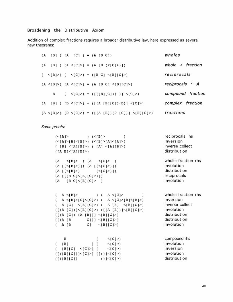
Broadening the Distributive Axiom

Addition of complex fractions requires a broader distributive law, here expressed as several

new theorems:

(A [B] ) (A [C] ) = (A [B C]) wholes

(A [B] ) (A <[C]>) = (A [B (<[C]>)]) whole + fraction

( <[B]>) ( <[C]>) = ([B C] <[B][C]>) r ec i p roca l s

(A <[B]>) (A <[C]>) = (A [B C] <[B][C]>) reciprocals * A

B ( <[C]>) = ([([B][C])( )] <[C]>) compound fraction

(A [B] ) (D <[C]>) = ([(A [B][C])(D)] <[C]>) complex fraction

(A <[B]>) (D <[C]>) = ([(A [B])(D [C])] <[B][C]>) f ract ions

Some proofs:

(<[A]> ) (<[B]> ) reciprocals lhs

(<[A]>[B]<[B]>) (<[B]>[A]<[A]>) inversion

( [B] <[A][B]>) ( [A] <[A][B]>) inverse collect

([A B]<[A][B]>) distribution

(A <[B]> ) (A <[C]> ) whole+fraction rhs

(A [(<[B]>)]) (A [(<[C]>)]) involution

(A [(<[B]>) (<[C]>)]) distribution

(A [([B C]<[B][C]>)]) reciprocals

(A [B C]<[B][C]> ) involution

( A <[B]> ) ( A <[C]> ) whole+fraction rhs

( A <[B]>[C]<[C]>) ( A <[C]>[B]<[B]>) inversion

( A [C] <[B][C]>) ( A [B] <[B][C]>) inverse collect

([(A [C])]<[B][C]>) ([(A [B])]<[B][C]>) involution

([(A [C]) (A [B])] <[B][C]>) distribution

([(A [B C])] <[B][C]>) distribution

( A [B C] <[B][C]>) involution

B ( <[C]>) compound rhs

( [B] ) ( <[C]>) involution

( [B][C] <[C]>) ( <[C]>) inversion

([([B][C])]<[C]>) ([()]<[C]>) involution

([([B][C]) ()]<[C]>) distribution

49

( A [B] ) ( D <[C]>) complex fraction rhs

( A [B][C] <[C]>) ( D <[C]>) inversion

([(A [B][C])]<[C]>) ([(D)] <[C]>) involution

([(A [B][C]) (D)] <[C]>) distribution

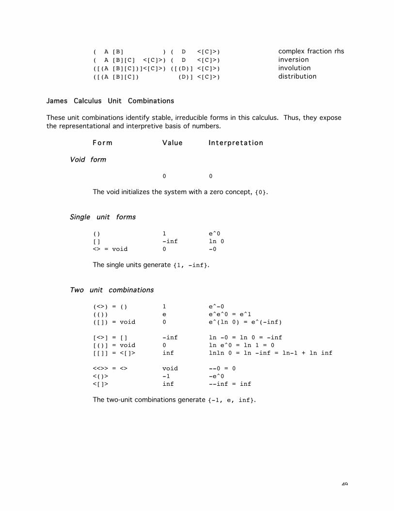
James Calculus Unit Combinations

These unit combinations identify stable, irreducible forms in this calculus. Thus, they expose

the representational and interpretive basis of numbers.

F o r m Value Interpretat ion

Void form

0 0

The void initializes the system with a zero concept, {0}.

Single unit forms

() 1 e^0[] -inf ln 0<> = void 0 -0

The single units generate {1, -inf}.

Two unit combinations

(<>) = () 1 e^-0(()) e e^e^0 = e^1([]) = void 0 e^(ln 0) = e^(-inf)

[<>] = [] -inf ln -0 = ln 0 = -inf[()] = void 0 ln e^0 = ln 1 = 0[[]] = <[]> inf lnln 0 = ln -inf = ln-1 + ln inf

<<>> = <> void --0 = 0<()> -1 -e^0<[]> inf --inf = inf

The two-unit combinations generate {-1, e, inf}.

50

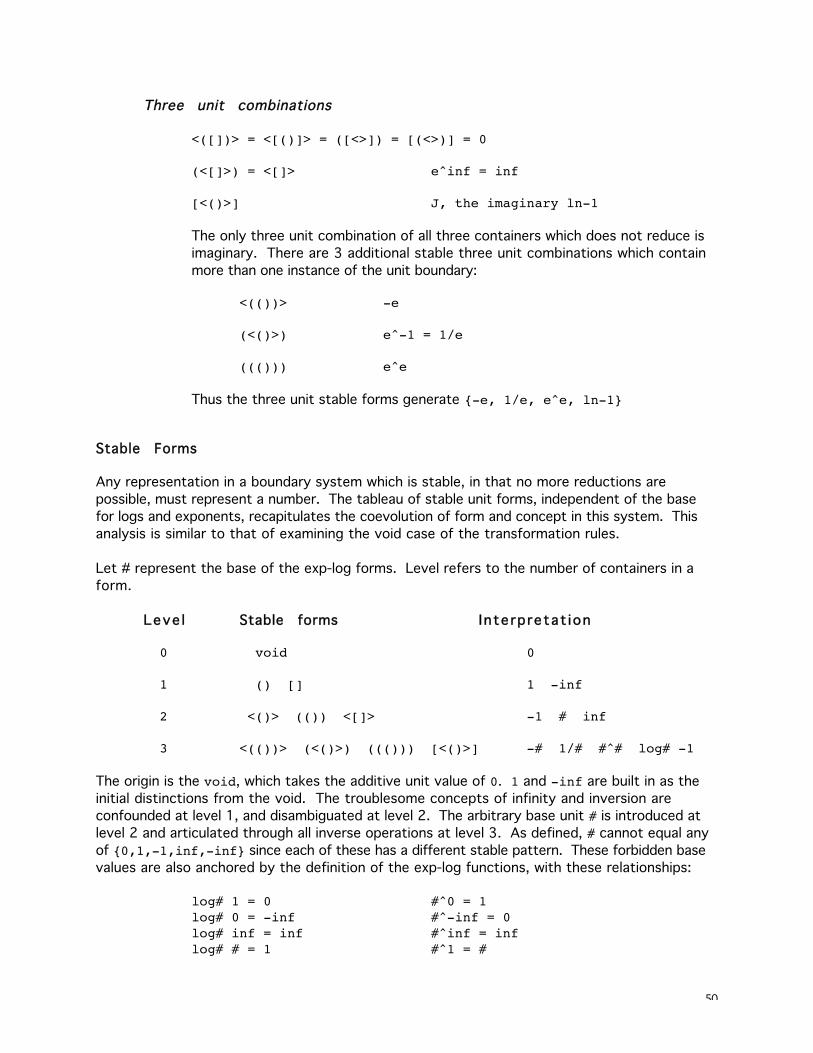
Three unit combinations

<([])> = <[()]> = ([<>]) = [(<>)] = 0

(<[]>) = <[]> eînf = inf

[<()>] J, the imaginary ln-1

The only three unit combination of all three containers which does not reduce is

imaginary. There are 3 additional stable three unit combinations which contain

more than one instance of the unit boundary:

<(())> -e

(<()>) e^-1 = 1/e

((())) eê

Thus the three unit stable forms generate {-e, 1/e, eê, ln-1}

Stable Forms

Any representation in a boundary system which is stable, in that no more reductions are

possible, must represent a number. The tableau of stable unit forms, independent of the base

for logs and exponents, recapitulates the coevolution of form and concept in this system. This

analysis is similar to that of examining the void case of the transformation rules.

Let # represent the base of the exp-log forms. Level refers to the number of containers in a

form.

Leve l Stable forms Interpretat ion

0 void 0

1 () [] 1 -inf

2 <()> (()) <[]> -1 # inf

3 <(())> (<()>) ((())) [<()>] -# 1/# #^# log# -1

The origin is the void, which takes the additive unit value of 0. 1 and -inf are built in as the

initial distinctions from the void. The troublesome concepts of infinity and inversion are

confounded at level 1, and disambiguated at level 2. The arbitrary base unit # is introduced at

level 2 and articulated through all inverse operations at level 3. As defined, # cannot equal any

of {0,1,-1,inf,-inf} since each of these has a different stable pattern. These forbidden base

values are also anchored by the definition of the exp-log functions, with these relationships:

log# 1 = 0 #^0 = 1log# 0 = -inf #^-inf = 0log# inf = inf #înf = inflog# # = 1 #^1 = #

51

These relationships indicate points in the log-exp functions which are independent of base.

Invalid bases can be assigned a meaning by treating them as imaginary. The equation which

permits movement between imaginary and real logarithms is

#^(log# x) = x

We can elect to interpret this equation as valid, again independent of the actual base. Thus #could any form, including the forbidden ones. We will now use this finesse to define logarithms

of negative numbers.

52

The James Imaginary

Introductory Comments

The quintessential imaginary number is i, the square root of minus one.

i = sqrt[-1]

i is the solution to the quadratic equation

i^2 = -1

Expressed as a self-referential equation,

i = -1/i = - (i^-1)

The imaginariness of i comes from the composition of two inverse operations, subtraction and

division. When the quadratic is equated to positive rather than negative unity, i represents a

standard unity:

i^2 = 1

i = {-1, 1}

In the self-referential equation, removal of the additive inverse expresses the same result:

i = + (i^-1) = 1/i

When the self-referential equation does not implicate the reciprocal of i, i becomes equal to

minus i, a role traditionally reserved for zero.

i = - (i^+1) = -i

Thus it appears that both the additive and the multiplicative inverses are required to identify

the imaginary unity.

The Boolean analog to the numerical i is the "square root of NOT" [Shoup], N. What Boolean

value, when composed with itself, is equal to the negation of itself?

N op N = not N

Self-referentially

N = N and not N

N = ((N)((N))) = ((N) N)

with the solution (the Kauffman-Varela imaginary)

N = not N

53

N = (N)

The Boolean imaginary oscillates with a cycle of two. The numerical i has a cycle of four:

i^0 = 1i^1 = ii^2 = -1i^3 = -ii^4 = 1

Strictly, this cycle is defined through successive multiplications, i, we might say, is the

multiplicative imaginary. Addition does not shift i through imaginary and real numerical

domains. Thus a complex number can be expressed as a sum of a real and an imaginary

component, with zero acting in its usual multiplicative role to orthogonalize the complex in

either domain:

1*1 + 0*i = 10*1 + 1*i = i

i is, in fact, a complex imaginary, a numerical composition of a simpler imaginary, the additive

imaginary, which we will label using J:

J = -J

J is not equal to zero, it is imaginary. We are restricted not to divide each side of the above

equation by 2 since the operation of division undermines the imaginary property of J.

What are the characteristics of this new imaginary? We will relate it to i, showing that i is a

particular combination of two Js; we will relate it to standard numerical operations, showing

that

J = ln -1

Accepting the above as a definition, we see that

e^J = e^(ln -1) = -1

That is,

i^2 = e^J

i = e^(J/2)

J = ln i^2 = 2 ln i

Some properties of J are proved below. The most interesting and fundamental of these is that Jdoes not equal 0, however it is its own additive inverse.

J = -J

54

That is,

J + J = 0

In the additive domain, J has a cycle of two:

J + 0 = JJ + J = 0J + -0 = JJ + -J = 0

We can now see that i is composed of two J cycles:

i^0 = (e^(J/2))^0 = e^0 = 1i^1 = (e^(J/2))^1 = e^(J^2) = ii^2 = (e^(J/2))^2 = e^J = -1i^3 = (e^(J/2))^3 = e^(3J/2) = e^(J + (J/2)) = e^J * e^(J/2) = -1 ii^4 = (e^(J/2))^4 = e^2J = e^0 = 1

J , Ln(-1)

Logarithms are defined for positive numbers only, since ln 0 = -infinity. Euler, in 1751,

defined logarithms of negative numbers as belonging to the complex domain. The exact

relationship is given by Euler's equation:

e^ib = cos b + i*sin b

ib = ln (cos b + i*sin b)

When b = PI we get

iPI = ln (-1 + i*0) = ln -1

The meaning of logarithms of negative numbers was widely discussed in the eighteenth century.

However, Euler's result seemed to resolve the questions: logs of negative numbers were

complex numbers.

The James imaginary, J, also addresses the logarithm of a negative number, but without

introducing complex numbers. When the angle b in Euler's equation rotates through 360degrees, or 2PI radians, it returns to its origin. A rotation of PI radians, 180 degrees, exactly

reverses the direction of the complex vector. Since sin 180 = 0, there is no i-imaginary

component to this rotation, thus no reference to i is necessary in this case. J represents this

specific rotation. Let

J = [<()>] = ln -1

A logarithm can be partitioned into a real and a J-imaginary part, the imaginary part carrying

the impact of a negative number on a logarithm:

ln -n = ln(n*-1) = ln n + ln -1 = ln n + J

55

Demonstration:

ln -5 = ln (5*-1) = ln 5 + ln -1 = (ln 5) + J

In boundary notation:

[<n>] = [([n][<()>])] = [n][<()>] = [n] J

Some properties of J are proved below using the same axioms as non-imaginaries. The most

interesting and fundamental of these is that J does not equal 0, however it is its own additive

inverse.

J = -J

That is,

J + J = 0

I l legal Transforms

Here is a simple demonstration of the generation of J from standard transforms:

0 = ln 1 = ln(-1*-1) = ln-1 + ln-1 = J + J = 0

Compare this to a similar transformation of the imaginary i:

1 = sqrt 1 = sqrt(-1*-1) = sqrt-1 * sqrt-1 = i*i = -1

Conventionally, we put a restriction on splitting 1 into -1 squared. There is no particular logic

to this other than if we allow it, then we can generate contradiction. Somehow, our

conceptualization of the imaginary i does not work as smoothly as it should.

The imaginary J manages this potential contradiction without restriction. For example:

ln(sqrt 1) = ln 1^(1/2) = (1/2)*ln 1 = (1/2)*ln(-1*-1)

= (1/2)*(J+J) = 0

Inverting the ln function by raising e to the power of the result (i.e. 0) restores the correct

answer of 1.

Due to the self-inverse property of J, care must be taken in using J, since the normal algebraic

operations do not remain consistent. For example,

J + J = 2J = 0

The problem is

2J = 0 does not imply J = 0/2 = 0

56

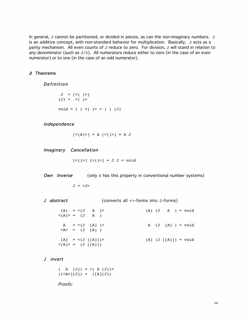
In general, J cannot be partitioned, or divided in pieces, as can the non-imaginary numbers. Jis an additive concept, with non-standard behavior for multiplication. Basically, J acts as a

parity mechanism. All even counts of J reduce to zero. For division, J will stand in relation to

any denominator (such as J/5). All numerators reduce either to zero (in the case of an even

numerator) or to one (in the case of an odd numerator).

J Theorems

Def i n i t i on

J = [<( )>](J) = <( )>

void = ( ) <( )> = ( ) (J)

Independence

[<(A)>] = A [<()>] = A J

Imaginary Cancellation

[<()>] [<()>] = J J = void

Own Inverse (only 0 has this property in conventional number systems)

J = <J>

J abstract (converts all <>-forms into J-forms)

(A) = <(J A )> (A) (J A ) = void<(A)> = (J A )

A = <(J [A] )> A (J [A] ) = void <A> = (J [A] )

[A] = <(J [[A]])> [A] (J [[A]]) = void<[A]> = (J [[A]])

J invert

( A [J]) = <( A [J])>([<A>][J]) = ([A][J])

Proofs:

57

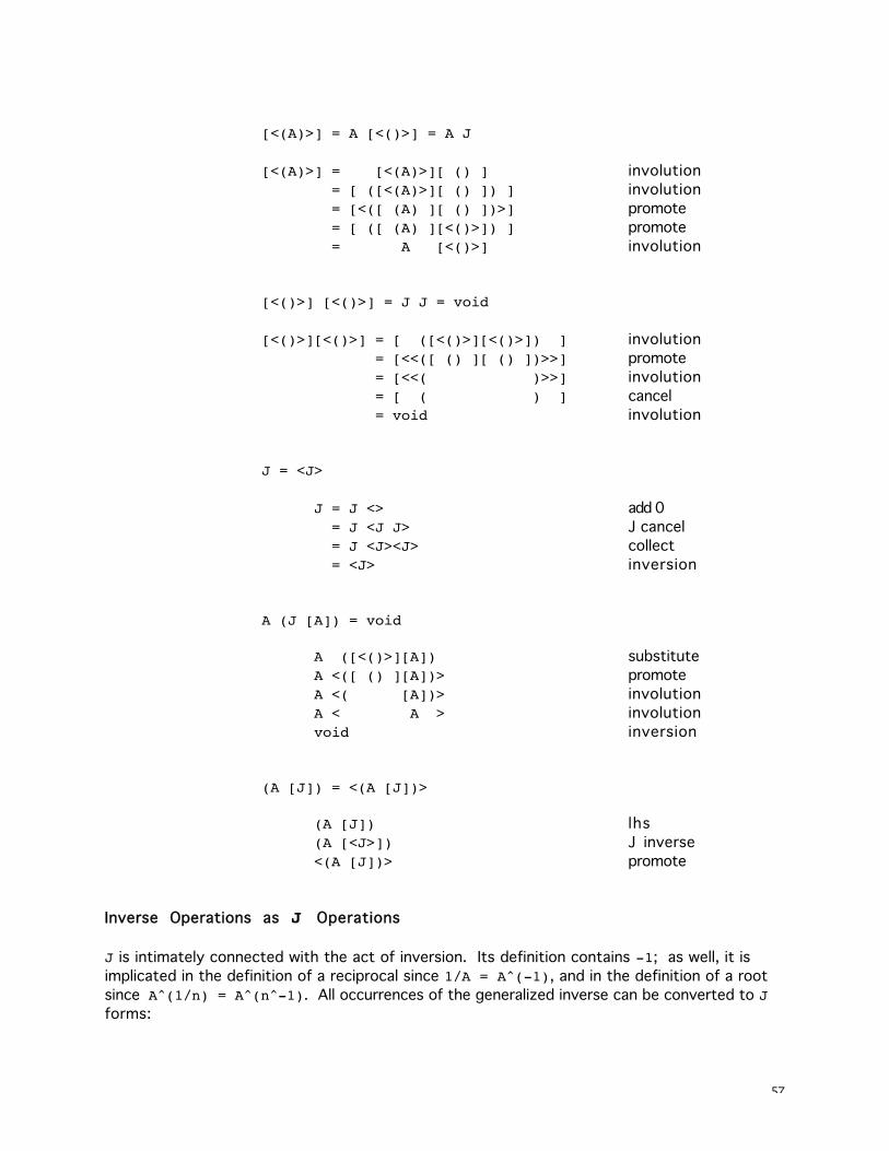
[<(A)>] = A [<()>] = A J

[<(A)>] = [<(A)>][ () ] involution

= [ ([<(A)>][ () ]) ] involution

= [<([ (A) ][ () ])>] promote

= [ ([ (A) ][<()>]) ] promote

= A [<()>] involution

[<()>] [<()>] = J J = void

[<()>][<()>] = [ ([<()>][<()>]) ] involution

= [<<([ () ][ () ])>>] promote

= [<<( )>>] involution

= [ ( ) ] cancel

= void involution

J = <J>

J = J <> add 0

= J <J J> J cancel

= J <J><J> collect

= <J> inversion

A (J [A]) = void

A ([<()>][A]) substitute

A <([ () ][A])> promote

A <( [A])> involution

A < A > involution

void inversion

(A [J]) = <(A [J])>

(A [J]) lhs

(A [<J>]) J inverse

<(A [J])> promote

Inverse Operations as J Operations

J is intimately connected with the act of inversion. Its definition contains -1; as well, it is

implicated in the definition of a reciprocal since 1/A = A^(-1), and in the definition of a root

since A^(1/n) = A^(n^-1). All occurrences of the generalized inverse can be converted to Jforms:

58

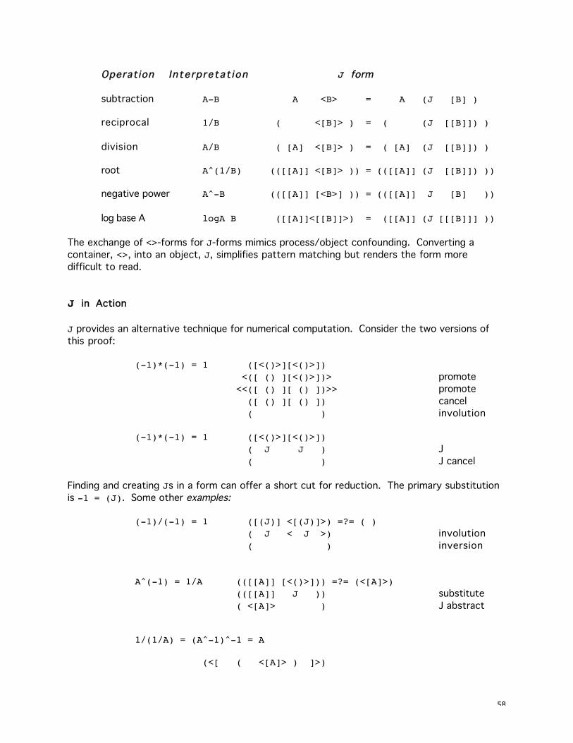
Operat ion Interpretat ion J form

subtraction A-B A = A (J [B] )

reciprocal 1/B ( <[B]> ) = ( (J [[B]]) )

division A/B ( [A] <[B]> ) = ( [A] (J [[B]]) )

root A^(1/B) (([[A]] <[B]> )) = (([[A]] (J [[B]]) ))

negative power A^-B (([[A]] [] )) = (([[A]] J [B] ))

log base A logA B ([[A]]<[[B]]>) = ([[A]] (J [[[B]]] ))

The exchange of <>-forms for J-forms mimics process/object confounding. Converting a

container, <>, into an object, J, simplifies pattern matching but renders the form more

difficult to read.

J in Action

J provides an alternative technique for numerical computation. Consider the two versions of

this proof:

(-1)*(-1) = 1 ([<()>][<()>]) <([ () ][<()>])> promote

<<([ () ][ () ])>> promote

([ () ][ () ]) cancel

( ) involution

(-1)*(-1) = 1 ([<()>][<()>]) ( J J ) J

( ) J cancel

Finding and creating Js in a form can offer a short cut for reduction. The primary substitution

is -1 = (J). Some other examples:

(-1)/(-1) = 1 ([(J)] <[(J)]>) =?= ( ) ( J < J >) involution

( ) inversion

A^(-1) = 1/A (([[A]] [<()>])) =?= (<[A]>)(([[A]] J )) substitute

( <[A]> ) J abstract

1/(1/A) = (A^-1)^-1 = A

(<[ ( <[A]> ) ]>)

59

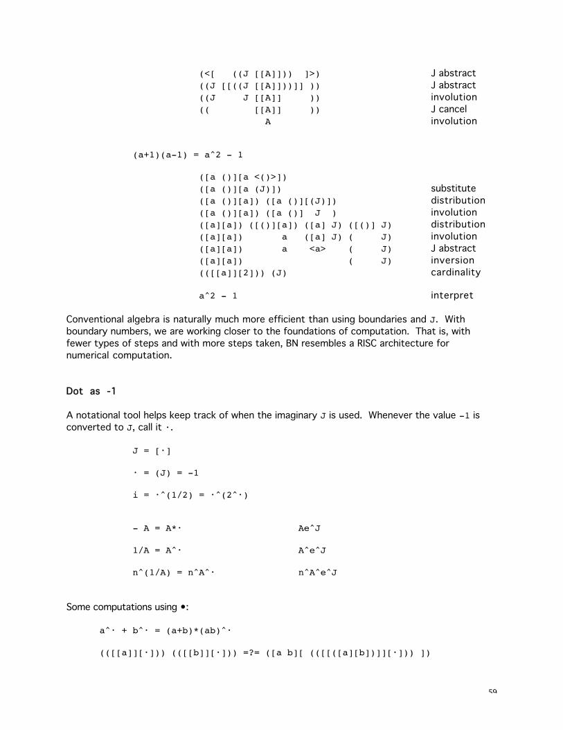
(<[ ((J [[A]])) ]>) J abstract

((J [[((J [[A]]))]] )) J abstract

((J J [[A]] )) involution

(( [[A]] )) J cancel

A involution

(a+1)(a-1) = a^2 - 1

([a ()][a <()>])([a ()][a (J)]) substitute

([a ()][a]) ([a ()][(J)]) distribution

([a ()][a]) ([a ()] J ) involution

([a][a]) ([()][a]) ([a] J) ([()] J) distribution

([a][a]) a ([a] J) ( J) involution

([a][a]) a <a> ( J) J abstract

([a][a]) ( J) inversion

(([[a]][2])) (J) cardinality

a^2 - 1 interpret

Conventional algebra is naturally much more efficient than using boundaries and J. With

boundary numbers, we are working closer to the foundations of computation. That is, with

fewer types of steps and with more steps taken, BN resembles a RISC architecture for

numerical computation.

Dot as -1

A notational tool helps keep track of when the imaginary J is used. Whenever the value -1 is

converted to J, call it •.

J = [•]

• = (J) = -1

i = •^(1/2) = •^(2^•)

- A = A*• Ae^J

1/A = A^• Aê^J

n^(1/A) = nÂ^• nÂê^J

Some computations using •:

a^• + b^• = (a+b)*(ab)^•

(([[a]][•])) (([[b]][•])) =?= ([a b][ (([[([a][b])]][•])) ])

60

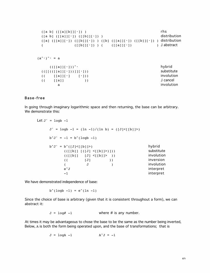
([a b] ([[a][b]][•]) ) rhs

([a b] ([[a]][•]) ([[b]][•]) ) distribution

([a] ([[a]][•]) ([[b]][•]) ) ([b] ([[a]][•]) ([[b]][•]) ) distribution

( ([[b]][•]) ) ( ([[a]][•]) ) J abstract

(a^•)^• = a

(([[a]][•]))^• hybrid

(([[(([[a]][•]))]][•])) substitute

(( [[a]][•] [•])) involution

(( [[a]] )) J cancel

a involution

Base - f r ee

In going through imaginary logarithmic space and then returning, the base can be arbitrary.

We demonstrate this:

Let J' = logb -1

J' = logb -1 = (ln -1)/(ln b) = ([J]<[[b]]>)

b^J' = -1 = b^(logb -1)

b^J' = b^([J]<[[b]]>) hybrid

(([[b]] [([J] <[[b]]>)])) substitute

(([[b]] [J] <[[b]]> )) involution

(( [J] )) inversion

( J ) involution

e^J interpret

-1 interpret

We have demonstrated independence of base:

b^(logb -1) = e^(ln -1)

Since the choice of base is arbitrary (given that it is consistent throughout a form), we can

abstract it:

J = log# -1 where # is any number.

At times it may be advantageous to chose the base to be the same as the number being inverted,

Below, A is both the form being operated upon, and the base of transformations; that is

J = logA -1 A^J = -1

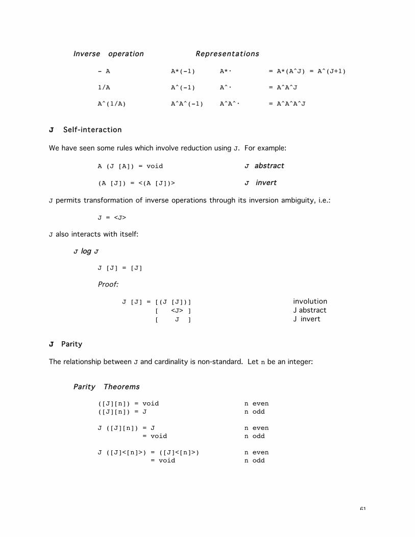
61

Inverse operation Representations

- A A*(-1) A*• = A*(A^J) = A^(J+1)

1/A A^(-1) A^• = AÂ^J

A^(1/A) AÂ^(-1) AÂ^• = AÂÂ^J

J Self-interaction

We have seen some rules which involve reduction using J. For example:

A (J [A]) = void J abstract

(A [J]) = <(A [J])> J invert

J permits transformation of inverse operations through its inversion ambiguity, i.e.:

J = <J>

J also interacts with itself:

J log J

J [J] = [J]

Proof:

J [J] = [(J [J])] involution

[ <J> ] J abstract

[ J ] J invert

J Parity

The relationship between J and cardinality is non-standard. Let n be an integer:

Parity Theorems

([J][n]) = void n even([J][n]) = J n odd

J ([J][n]) = J n even = void n odd

J ([J]<[n]>) = ([J]<[n]>) n even = void n odd

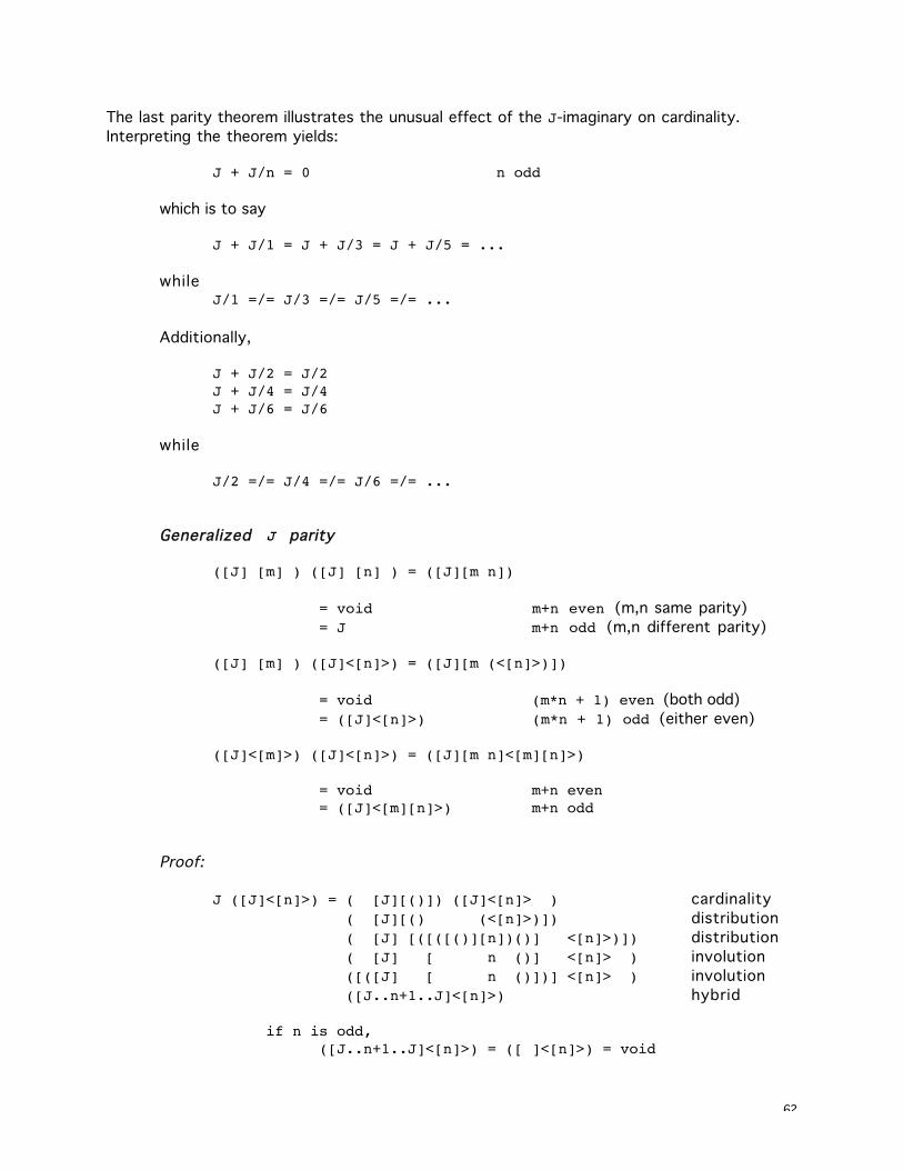
62

The last parity theorem illustrates the unusual effect of the J-imaginary on cardinality.

Interpreting the theorem yields:

J + J/n = 0 n odd

which is to say

J + J/1 = J + J/3 = J + J/5 = ...

whileJ/1 =/= J/3 =/= J/5 =/= ...

Additionally,

J + J/2 = J/2J + J/4 = J/4J + J/6 = J/6

while

J/2 =/= J/4 =/= J/6 =/= ...

Generalized J parity

([J] [m] ) ([J] [n] ) = ([J][m n])

= void m+n even (m,n same parity)

= J m+n odd (m,n different parity)

([J] [m] ) ([J]<[n]>) = ([J][m (<[n]>)])

= void (m*n + 1) even (both odd)

= ([J]<[n]>) (m*n + 1) odd (either even)

([J]<[m]>) ([J]<[n]>) = ([J][m n]<[m][n]>)

= void m+n even= ([J]<[m][n]>) m+n odd

Proof:

J ([J]<[n]>) = ( [J][()]) ([J]<[n]> ) cardinality

( [J][() (<[n]>)]) distribution

( [J] [([([()][n])()] <[n]>)]) distribution

( [J] [ n ()] <[n]> ) involution

([([J] [ n ()])] <[n]> ) involution

([J..n+1..J]<[n]>) hybrid

if n is odd,([J..n+1..J]<[n]>) = ([ ]<[n]>) = void

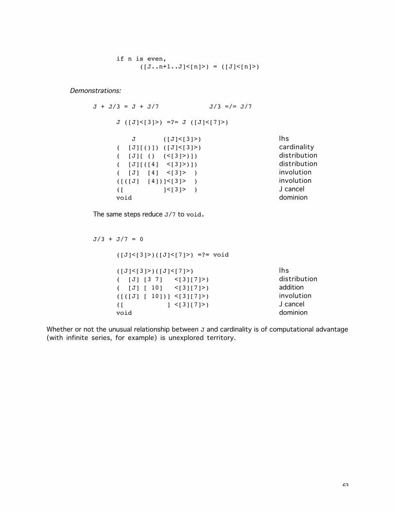
63

if n is even,([J..n+1..J]<[n]>) = ([J]<[n]>)

Demonstrations:

J + J/3 = J + J/7 J/3 =/= J/7

J ([J]<[3]>) =?= J ([J]<[7]>)

J ([J]<[3]>) lhs

( [J][()]) ([J]<[3]>) cardinality

( [J][ () (<[3]>)]) distribution

( [J][([4] <[3]>)]) distribution

( [J] [4] <[3]> ) involution

([([J] [4])]<[3]> ) involution

([ ]<[3]> ) J cancel

void dominion

The same steps reduce J/7 to void.

J/3 + J/7 = 0

([J]<[3]>)([J]<[7]>) =?= void

([J]<[3]>)([J]<[7]>) lhs

( [J] [3 7] <[3][7]>) distribution

( [J] [ 10] <[3][7]>) addition

([([J] [ 10])] <[3][7]>) involution

([ ] <[3][7]>) J cancel

void dominion

Whether or not the unusual relationship between J and cardinality is of computational advantage

(with infinite series, for example) is unexplored territory.

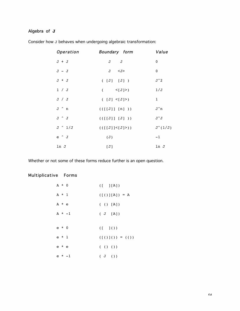
64

Algebra of J

Consider how J behaves when undergoing algebraic transformation:

Operat ion Boundary form Value

J + J J J 0

J - J J <J> 0

J * J ( [J] [J] ) J^2

1 / J ( <[J]>) 1/J

J / J ( [J] <[J]>) 1

J ^ n (([[J]] [n] )) J^n

J ^ J (([[J]] [J] )) J^J

J ^ 1/J (([[J]]<[J]>)) J^(1/J)

e ^ J (J) -1

ln J [J] ln J

Whether or not some of these forms reduce further is an open question.

Multipl icative Forms

A * 0 ([ ][A])

A * 1 ([()][A]) = A

A * e ( () [A])

A * -1 ( J [A])

e * 0 ([ ]())

e * 1 ([()]()) = (())

e * e ( () ())

e * -1 ( J ())

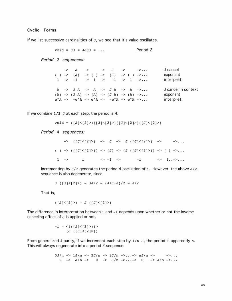
65

Cyclic Forms

If we list successive cardinalities of J, we see that it's value oscillates.

void = JJ = JJJJ = ... Period 2

Period 2 sequences:

-> J -> -> J -> ->... J cancel

( ) -> (J) -> ( ) -> (J) -> ( ) ->... exponent

1 -> -1 -> 1 -> -1 -> 1 ->... interpret

A -> J A -> A -> J A -> A ->... J cancel in context

(A) -> (J A) -> (A) -> (J A) -> (A) ->... exponent

eÂ -> -eÂ -> eÂ -> -eÂ -> eÂ ->... interpret

If we combine 1/2 J at each step, the period is 4:

void = ([J]<[2]>)([J]<[2]>)([J]<[2]>)([J]<[2]>)

Period 4 sequences:

-> ([J]<[2]>) -> J -> J ([J]<[2]>) -> ->...

( ) -> (([J]<[2]>)) -> (J) -> (J ([J]<[2]>)) -> ( ) ->...

1 -> i -> -1 -> -i -> 1..->...

Incrementing by J/2 generates the period 4 oscillation of i. However, the above J/2sequence is also degenerate, since

J ([J]<[2]>) = 3J/2 = (J+J+J)/2 = J/2

That is,

([J]<[2]>) = J ([J]<[2]>)

The difference in interpretation between i and -i depends upon whether or not the inverse

canceling effect of J is applied or not.

-i = <(([J]<[2]>))> (J ([J]<[2]>))

From generalized J parity, if we increment each step by 1/n J, the period is apparently n.

This will always degenerate into a period 2 sequence:

0J/n -> 1J/n -> 2J/n -> 3J/n ->...-> nJ/n -> ->... 0 -> J/n -> 0 -> J/n ->...-> 0 -> J/n ->...

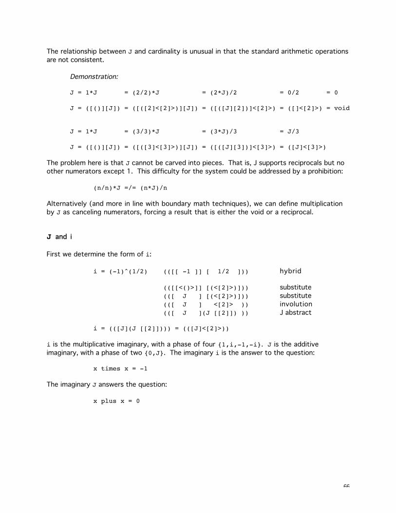
66

The relationship between J and cardinality is unusual in that the standard arithmetic operations

are not consistent.

Demonstration:

J = 1*J = (2/2)*J = (2*J)/2 = 0/2 = 0

J = ([()][J]) = ([([2]<[2]>)][J]) = ([([J][2])]<[2]>) = ([]<[2]>) = void

J = 1*J = (3/3)*J = (3*J)/3 = J/3

J = ([()][J]) = ([([3]<[3]>)][J]) = ([([J][3])]<[3]>) = ([J]<[3]>)

The problem here is that J cannot be carved into pieces. That is, J supports reciprocals but no

other numerators except 1. This difficulty for the system could be addressed by a prohibition:

(n/n)*J =/= (n*J)/n

Alternatively (and more in line with boundary math techniques), we can define multiplication

by J as canceling numerators, forcing a result that is either the void or a reciprocal.

J and i

First we determine the form of i:

i = (-1)^(1/2) (([[ -1 ]] [ 1/2 ])) hybrid

(([[<()>]] [(<[2]>)])) substitute

(([ J ] [(<[2]>)])) substitute

(([ J ] <[2]> )) involution

(([ J ](J [[2]]) )) J abstract

i = (([J](J [[2]]))) = (([J]<[2]>))

i is the multiplicative imaginary, with a phase of four {1,i,-1,-i}. J is the additive

imaginary, with a phase of two {0,J}. The imaginary i is the answer to the question:

x times x = -1

The imaginary J answers the question:

x plus x = 0

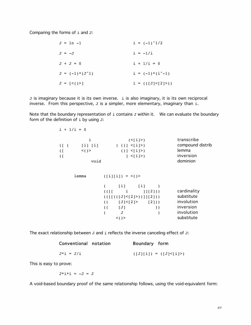
67

Comparing the forms of i and J:

J = ln -1 i = (-1)^1/2

J = -J i = -1/i

J + J = 0 i + 1/i = 0

J = (-1)*(J^1) i = (-1)*(i^-1)

J = [<()>] i = (([J]<[2]>))

J is imaginary because it is its own inverse. i is also imaginary, it is its own reciprocal

inverse. From this perspective, J is a simpler, more elementary, imaginary than i.

Note that the boundary representation of i contains J within it. We can evaluate the boundary

form of the definition of i by using J:

i + 1/i = 0

i (<[i]>) transcribe

([ ( [i] [i] ) ()] <[i]>) compound distrib

([ <()> ()] <[i]>) lemma

([ ] <[i]>) inversion

void dominion

lemma ([i][i]) = <()>

( [i] [i] )(([[ i ]][2])) cardinality

(([[(([J]<[2]>))]][2])) substitute

(( [J]<[2]> [2])) involution

(( [J] )) inversion

( J ) involution

<()> substitute

The exact relationship between J and i reflects the inverse canceling effect of J:

Conventional notation Boundary form

J*i = J/i ([J][i]) = ([J]<[i]>)

This is easy to prove:

J*i*i = -J = J

A void-based boundary proof of the same relationship follows, using the void-equivalent form:

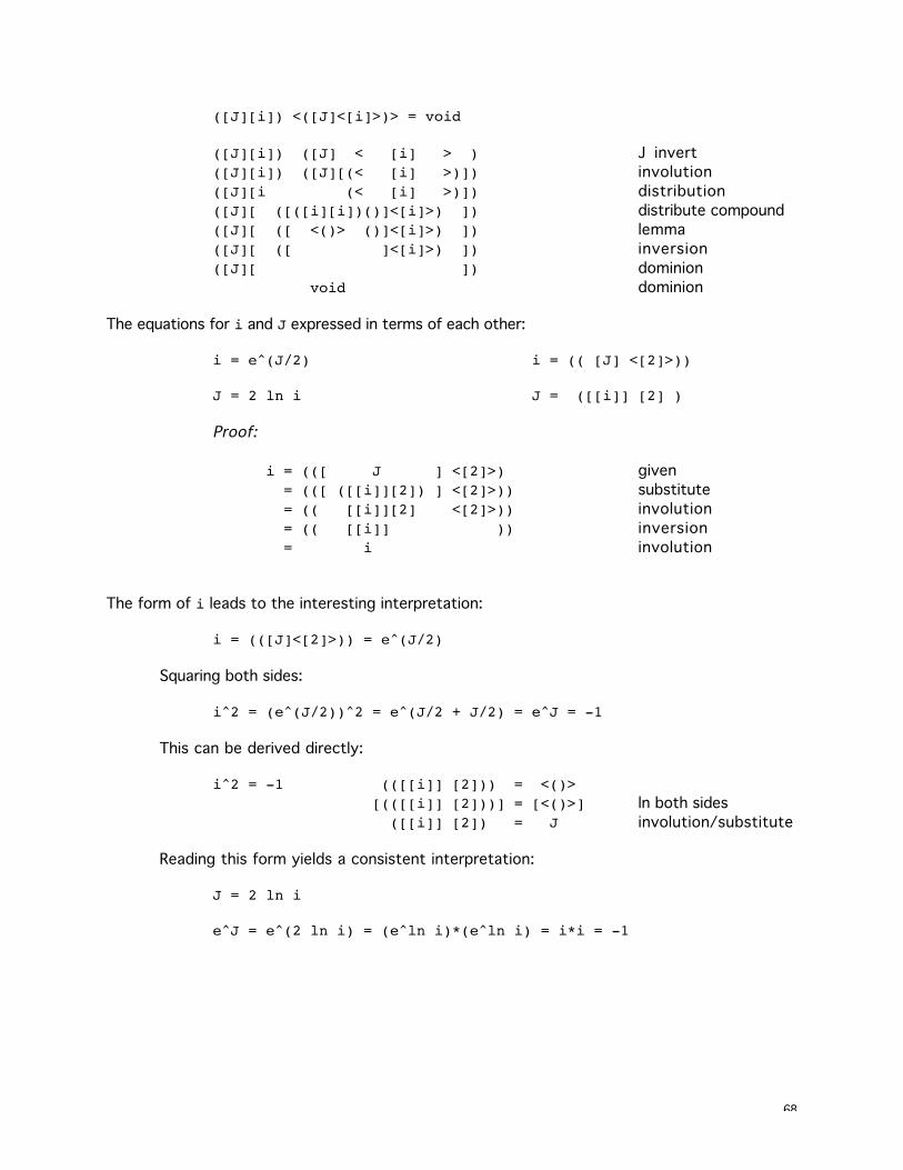
68

([J][i]) <([J]<[i]>)> = void

([J][i]) ([J] < [i] > ) J invert

([J][i]) ([J][(< [i] >)]) involution

([J][i (< [i] >)]) distribution

([J][ ([([i][i])()]<[i]>) ]) distribute compound

([J][ ([ <()> ()]<[i]>) ]) lemma

([J][ ([ ]<[i]>) ]) inversion

([J][ ]) dominion

void dominion

The equations for i and J expressed in terms of each other:

i = e^(J/2) i = (( [J] <[2]>))

J = 2 ln i J = ([[i]] [2] )

Proof:

i = (([ J ] <[2]>) given

= (([ ([[i]][2]) ] <[2]>)) substitute

= (( [[i]][2] <[2]>)) involution

= (( [[i]] )) inversion

= i involution

The form of i leads to the interesting interpretation:

i = (([J]<[2]>)) = e^(J/2)

Squaring both sides:

i^2 = (e^(J/2))^2 = e^(J/2 + J/2) = e^J = -1

This can be derived directly:

i^2 = -1 (([[i]] [2])) = <()>[(([[i]] [2]))] = [<()>] ln both sides

([[i]] [2]) = J involution/substitute

Reading this form yields a consistent interpretation:

J = 2 ln i

e^J = e^(2 ln i) = (e^ln i)*(e^ln i) = i*i = -1

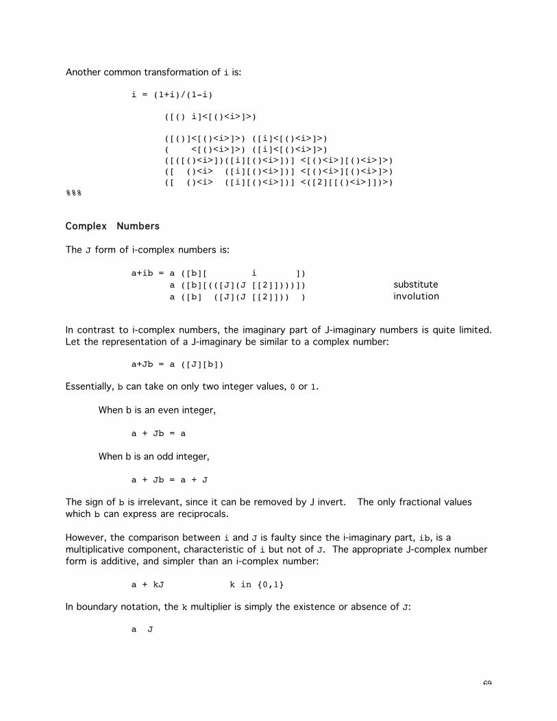
69

Another common transformation of i is:

i = (1+i)/(1-i)

([() i]<[()]>)

([()]<[()]>) ([i]<[()]>)( <[()]>) ([i]<[()]>)([([()])([i][()])] <[()][()]>)([ () ([i][()])] <[()][()]>)([ () ([i][()])] <([2][[()]])>)

%%%

Complex Numbers

The J form of i-complex numbers is:

a+ib = a ([b][ i ]) a ([b][(([J](J [[2]])))]) substitute

a ([b] ([J](J [[2]])) ) involution

In contrast to i-complex numbers, the imaginary part of J-imaginary numbers is quite limited.

Let the representation of a J-imaginary be similar to a complex number:

a+Jb = a ([J][b])

Essentially, b can take on only two integer values, 0 or 1.

When b is an even integer,

a + Jb = a

When b is an odd integer,

a + Jb = a + J

The sign of b is irrelevant, since it can be removed by J invert. The only fractional values

which b can express are reciprocals.

However, the comparison between i and J is faulty since the i-imaginary part, ib, is a

multiplicative component, characteristic of i but not of J. The appropriate J-complex number

form is additive, and simpler than an i-complex number:

a + kJ k in {0,1}

In boundary notation, the k multiplier is simply the existence or absence of J:

a J

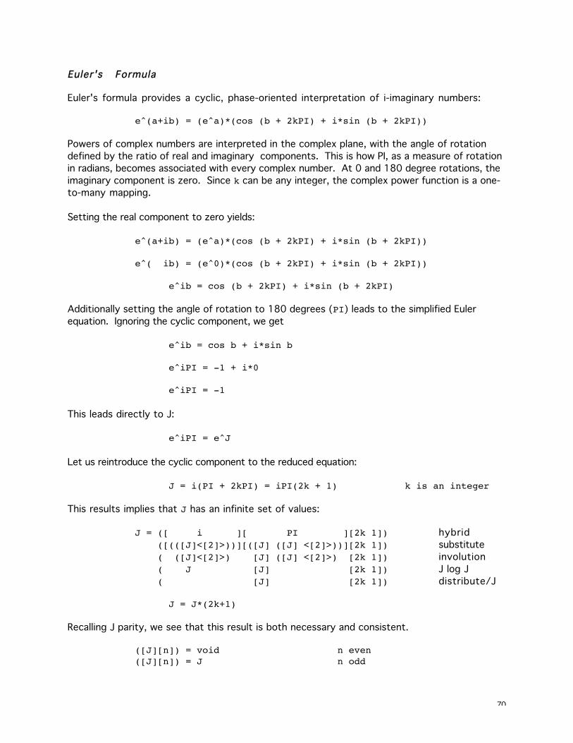
70

Euler's Formula

Euler's formula provides a cyclic, phase-oriented interpretation of i-imaginary numbers:

e^(a+ib) = (eâ)*(cos (b + 2kPI) + i*sin (b + 2kPI))

Powers of complex numbers are interpreted in the complex plane, with the angle of rotation

defined by the ratio of real and imaginary components. This is how PI, as a measure of rotation

in radians, becomes associated with every complex number. At 0 and 180 degree rotations, the

imaginary component is zero. Since k can be any integer, the complex power function is a one-

to-many mapping.

Setting the real component to zero yields:

e^(a+ib) = (eâ)*(cos (b + 2kPI) + i*sin (b + 2kPI))

e^( ib) = (e^0)*(cos (b + 2kPI) + i*sin (b + 2kPI))

eîb = cos (b + 2kPI) + i*sin (b + 2kPI)

Additionally setting the angle of rotation to 180 degrees (PI) leads to the simplified Euler

equation. Ignoring the cyclic component, we get

eîb = cos b + i*sin b

eîPI = -1 + i*0

eîPI = -1

This leads directly to J:

eîPI = e^J

Let us reintroduce the cyclic component to the reduced equation:

J = i(PI + 2kPI) = iPI(2k + 1) k is an integer

This results implies that J has an infinite set of values:

J = ([ i ][ PI ][2k 1]) hybrid

([(([J]<[2]>))][([J] ([J] <[2]>))][2k 1]) substitute

( ([J]<[2]>) [J] ([J] <[2]>) [2k 1]) involution

( J [J] [2k 1]) J log J

( [J] [2k 1]) distribute/J

J = J*(2k+1)

Recalling J parity, we see that this result is both necessary and consistent.

([J][n]) = void n even([J][n]) = J n odd

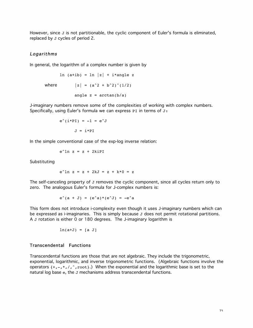
71

However, since J is not partitionable, the cyclic component of Euler's formula is eliminated,

replaced by J cycles of period 2.

Logar i thms

In general, the logarithm of a complex number is given by

ln (a+ib) = ln |z| + i*angle z

where |z| = (a^2 + b^2)^(1/2)

angle z = arctan(b/a)

J-imaginary numbers remove some of the complexities of working with complex numbers.

Specifically, using Euler's formula we can express PI in terms of J:

e^(i*PI) = -1 = e^J

J = i*PI

In the simple conventional case of the exp-log inverse relation:

e^ln z = z + 2kiPI

Substituting

e^ln z = z + 2kJ = z + k*0 = z

The self-canceling property of J removes the cyclic component, since all cycles return only to

zero. The analogous Euler's formula for J-complex numbers is:

e^(a + J) = (e^a)*(e^J) = -e^a

This form does not introduce i-complexity even though it uses J-imaginary numbers which can

be expressed as i-imaginaries. This is simply because J does not permit rotational partitions.

A J rotation is either 0 or 180 degrees. The J-imaginary logarithm is

ln(a+J) = [a J]

Transcendental Functions

Transcendental functions are those that are not algebraic. They include the trigonometric,

exponential, logarithmic, and inverse trigonometric functions. (Algebraic functions involve the

operators {+,-,*,/,^,root}.) When the exponential and the logarithmic base is set to the

natural log base e, the J mechanisms address transcendental functions.

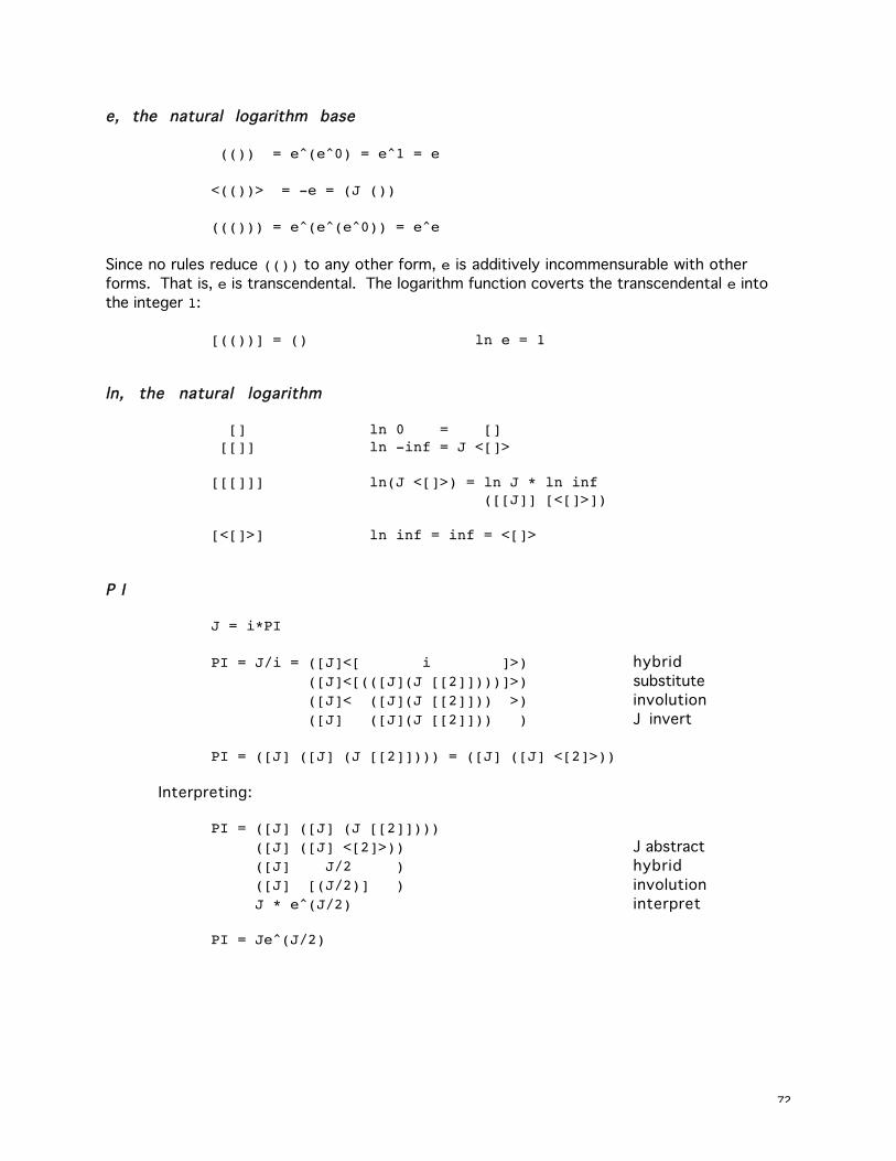
72

e, the natural logarithm base

(()) = e^(e^0) = e^1 = e

<(())> = -e = (J ())

((())) = e^(e^(e^0)) = e^e

Since no rules reduce (()) to any other form, e is additively incommensurable with other

forms. That is, e is transcendental. The logarithm function coverts the transcendental e into

the integer 1:

[(())] = () ln e = 1

ln, the natural logarithm

[] ln 0 = [] [[]] ln -inf = J <[]>

[[[]]] ln(J <[]>) = ln J * ln inf ([[J]] [<[]>])

[<[]>] ln inf = inf = <[]>

P I

J = i*PI

PI = J/i = ([J]<[ i ]>) hybrid

([J]<[(([J](J [[2]])))]>) substitute

([J]< ([J](J [[2]])) >) involution

([J] ([J](J [[2]])) ) J invert

PI = ([J] ([J] (J [[2]]))) = ([J] ([J] <[2]>))

Interpreting:

PI = ([J] ([J] (J [[2]]))) ([J] ([J] <[2]>)) J abstract

([J] J/2 ) hybrid

([J] [(J/2)] ) involution

J * e^(J/2) interpret

PI = Je^(J/2)

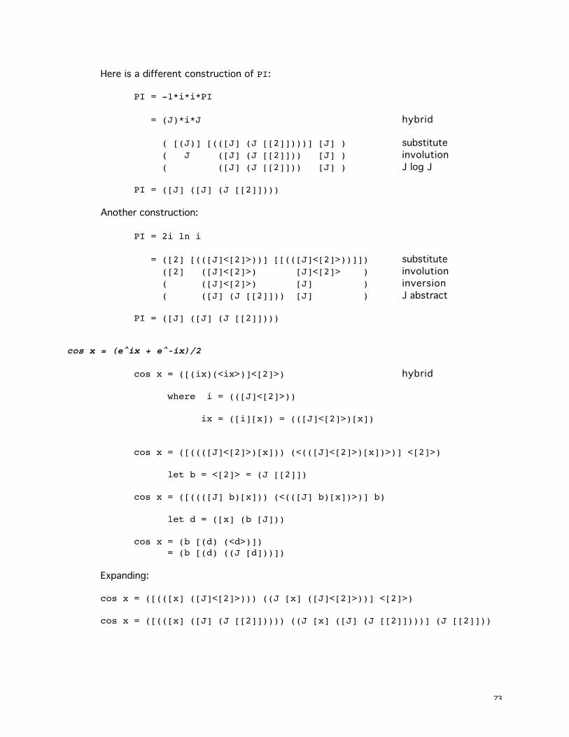
73

Here is a different construction of PI:

PI = -1*i*i*PI

= (J)*i*J hybrid

( [(J)] [(([J] (J [[2]])))] [J] ) substitute

( J ([J] (J [[2]])) [J] ) involution

( ([J] (J [[2]])) [J] ) J log J

PI = ([J] ([J] (J [[2]])))

Another construction:

PI = 2i ln i

= ([2] [(([J]<[2]>))] [[(([J]<[2]>))]]) substitute

([2] ([J]<[2]>) [J]<[2]> ) involution

( ([J]<[2]>) [J] ) inversion

( ([J] (J [[2]])) [J] ) J abstract

PI = ([J] ([J] (J [[2]])))

cos x = (e^ix + e^-ix)/2

cos x = ([(ix)(<ix>)]<[2]>) hybrid

where i = (([J]<[2]>))

ix = ([i][x]) = (([J]<[2]>)[x])

cos x = ([((([J]<[2]>)[x])) (<(([J]<[2]>)[x])>)] <[2]>)

let b = <[2]> = (J [[2]])

cos x = ([((([J] b)[x])) (<(([J] b)[x])>)] b)

let d = ([x] (b [J]))

cos x = (b [(d) (<d>)])= (b [(d) ((J [d]))])

Expanding:

cos x = ([(([x] ([J]<[2]>))) ((J [x] ([J]<[2]>))] <[2]>)

cos x = ([(([x] ([J] (J [[2]])))) ((J [x] ([J] (J [[2]])))] (J [[2]]))

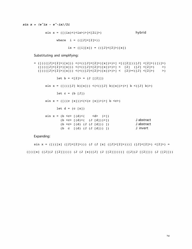
74

sin x = (e^ix - e^-ix)/2i

sin x = ([(ix)<(<ix>)>]<[2i]>) hybrid

where i = (([J]<[2]>))

ix = ([i][x]) = (([J]<[2]>)[x])

Substituting and simplifying:

= ([((([J]<[2]>)[x])) <(<(([J]<[2]>)[x])>)>] <[([2][(([J] <[2]>))])]>) ([((([J]<[2]>)[x])) <(<(([J]<[2]>)[x])>)>] < [2] ([J] <[2]>) >) ([((([J]<[2]>)[x])) <(<(([J]<[2]>)[x])>)>] < [2]><([J] <[2]>) >)

let b = <[2]> = (J [[2]])

sin x = ([((([J] b)[x])) <(<(([J] b)[x])>)>] b <([J] b)>)

let c = (b [J])

sin x = ([((c [x]))<(<(c [x])>)>] b <c>)

let d = (c [x])

sin x = (b <c> [(d)<( <d> )>]) (b <c> [(d)<( (J [d]))>]) J abstract

(b <c> [(d) (J (J [d])) ]) J abstract

(b c [(d) (J (J [d])) ]) J invert

Expanding:

sin x = ([(([x] ([J]<[2]>))) (J (J [x] ([J]<[2]>)))] ([J]<[2]>) <[2]>) =

([(([x] ([J](J [[2]])))) (J (J [x]([J] (J [[2]]))))] ([J](J [[2]])) (J [[2]]))

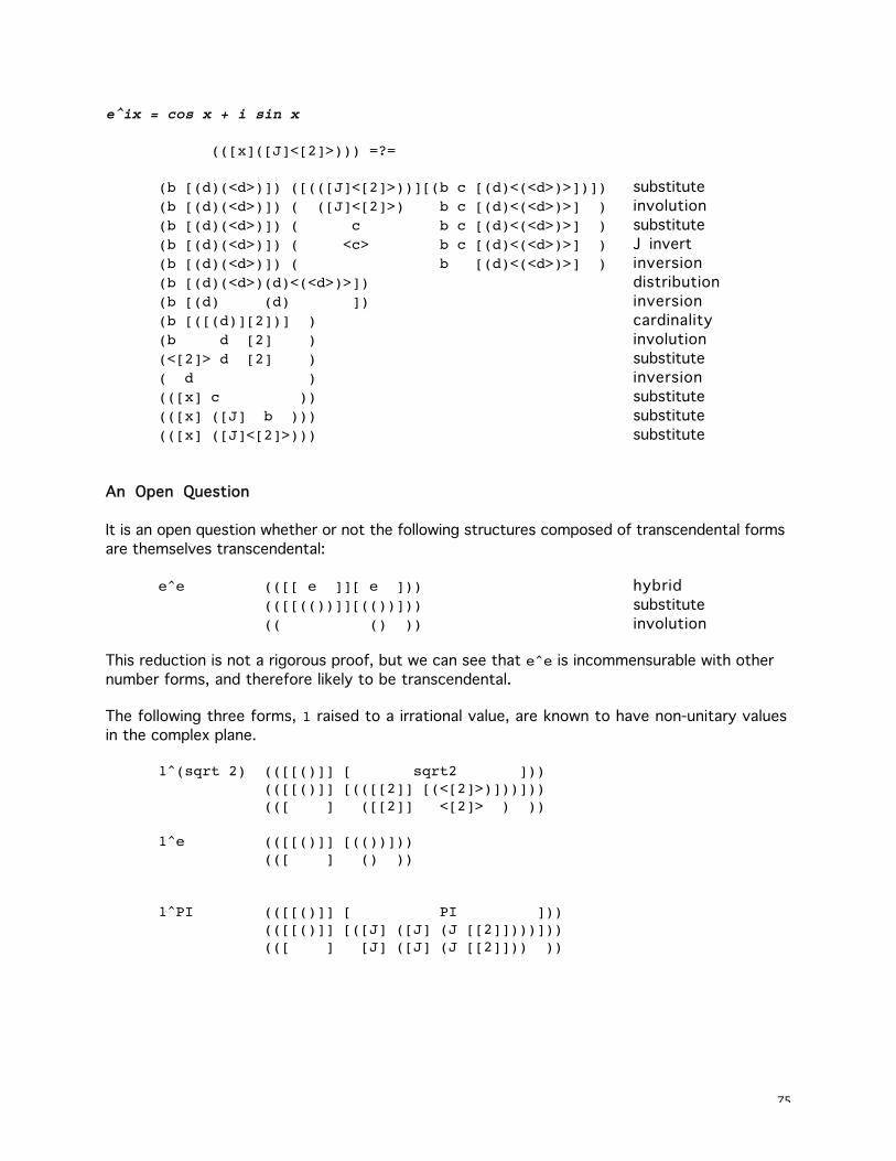
75

eîx = cos x + i sin x

(([x]([J]<[2]>))) =?=

(b [(d)(<d>)]) ([(([J]<[2]>))][(b c [(d)<(<d>)>])]) substitute

(b [(d)(<d>)]) ( ([J]<[2]>) b c [(d)<(<d>)>] ) involution

(b [(d)(<d>)]) ( c b c [(d)<(<d>)>] ) substitute

(b [(d)(<d>)]) ( <c> b c [(d)<(<d>)>] ) J invert

(b [(d)(<d>)]) ( b [(d)<(<d>)>] ) inversion

(b [(d)(<d>)(d)<(<d>)>]) distribution

(b [(d) (d) ]) inversion

(b [([(d)][2])] ) cardinality

(b d [2] ) involution

(<[2]> d [2] ) substitute

( d ) inversion

(([x] c )) substitute

(([x] ([J] b ))) substitute

(([x] ([J]<[2]>))) substitute

An Open Question

It is an open question whether or not the following structures composed of transcendental forms

are themselves transcendental:

eê (([[ e ]][ e ])) hybrid

(([[(())]][(())])) substitute

(( () )) involution

This reduction is not a rigorous proof, but we can see that eê is incommensurable with other

number forms, and therefore likely to be transcendental.

The following three forms, 1 raised to a irrational value, are known to have non-unitary values

in the complex plane.

1^(sqrt 2) (([[()]] [ sqrt2 ]))(([[()]] [(([[2]] [(<[2]>)]))]))(([ ] ([[2]] <[2]> ) ))

1ê (([[()]] [(())]))(([ ] () ))

1^PI (([[()]] [ PI ]))(([[()]] [([J] ([J] (J [[2]])))]))(([ ] [J] ([J] (J [[2]])) ))

76

It is not known whether or not the following two forms reduce further.

PI^e (([[ PI ]] [ e ]))(([[([J] ([J]<[[2]]>))]] [(())])) substitute

(([ [J] ([J]<[[2]]>) ] () )) involution

PI^PI (([[ PI ]][ PI ]))(([[([J] ([J]<[[2]]>))]][([J] ([J]<[[2]]>))])) substitute

(([ [J] ([J]<[[2]]>) ] [J] ([J]<[[2]]>) )) involution

Axioms of Infinity

The interaction between infinity and form requires new theorems. These absorption rules

define when an infinite form absorbs, or renders void, other forms sharing the same space.

Negative Dominion cannot be proved, it is an axiom. The other reduction rules for infinity are

derived from the Dominion axiom.

Negative Infinity

A [] = [] dominion, any A

([]) = void involution of negative infinity

[[]] = J <[]> log of negative infinity

Positive Infinity

A <[]> = <[]> positive dominion, A not in {[],J}

(<[]>) = <[]> infinite exponent

[<[]>] = <[]> infinite log

Proofs:

[[]] = J <[]> loglog 0

[ [] ][< <[]> >] inverse cancel

[<(J [ [] ])>] J abstract

[ (J [<[]>]) ] inverse promote

J [<[]>] involution

The implication from this result is that

[[]] = J <[]> =/= <[]>

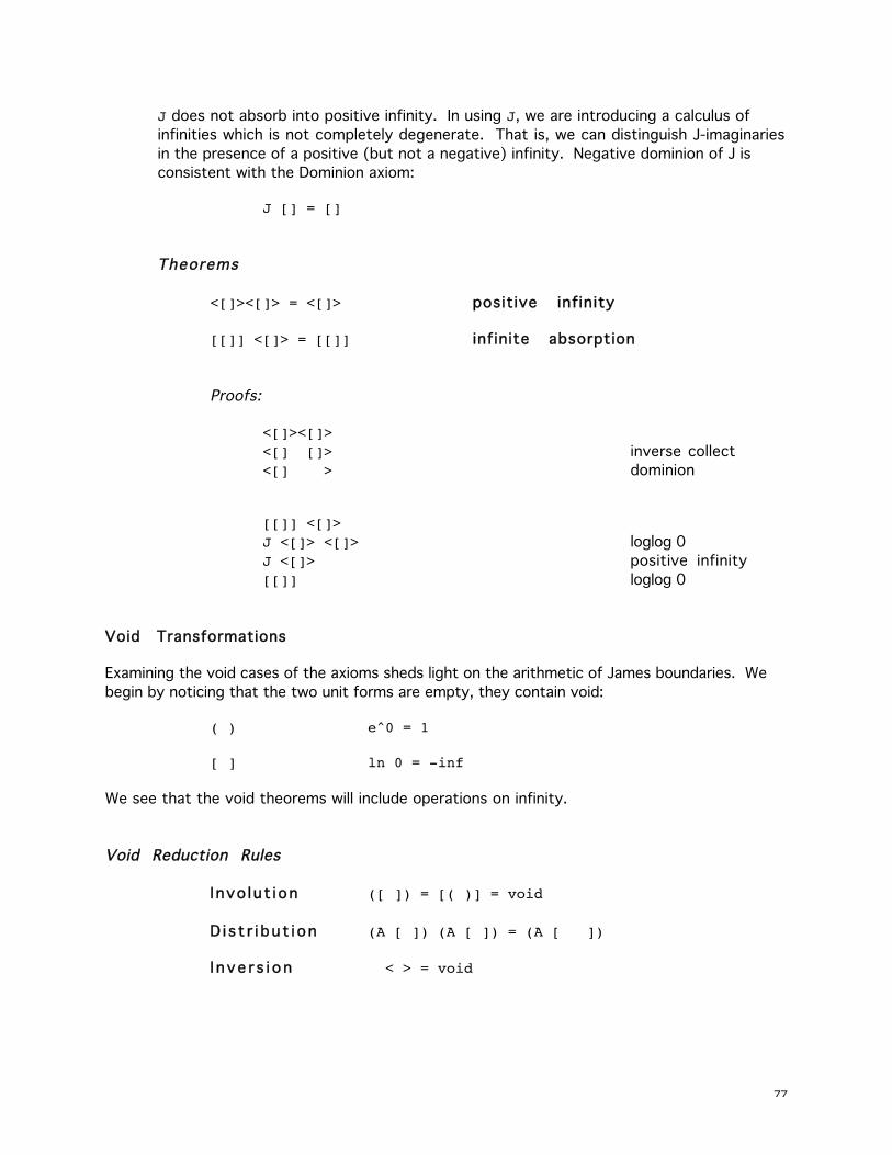
77

J does not absorb into positive infinity. In using J, we are introducing a calculus of

infinities which is not completely degenerate. That is, we can distinguish J-imaginaries

in the presence of a positive (but not a negative) infinity. Negative dominion of J is

consistent with the Dominion axiom:

J [] = []

Theorems

<[]><[]> = <[]> positive infinity

[[]] <[]> = [[]] infinite absorption

Proofs:

<[]><[]><[] []> inverse collect

<[] > dominion

[[]] <[]>J <[]> <[]> loglog 0

J <[]> positive infinity

[[]] loglog 0

Void Transformations

Examining the void cases of the axioms sheds light on the arithmetic of James boundaries. We

begin by noticing that the two unit forms are empty, they contain void:

( ) e^0 = 1

[ ] ln 0 = -inf

We see that the void theorems will include operations on infinity.

Void Reduction Rules

I nvo lu t i on ([ ]) = [( )] = void

D i s t r i bu t i on (A [ ]) (A [ ]) = (A [ ])

I n v e r s i o n < > = void

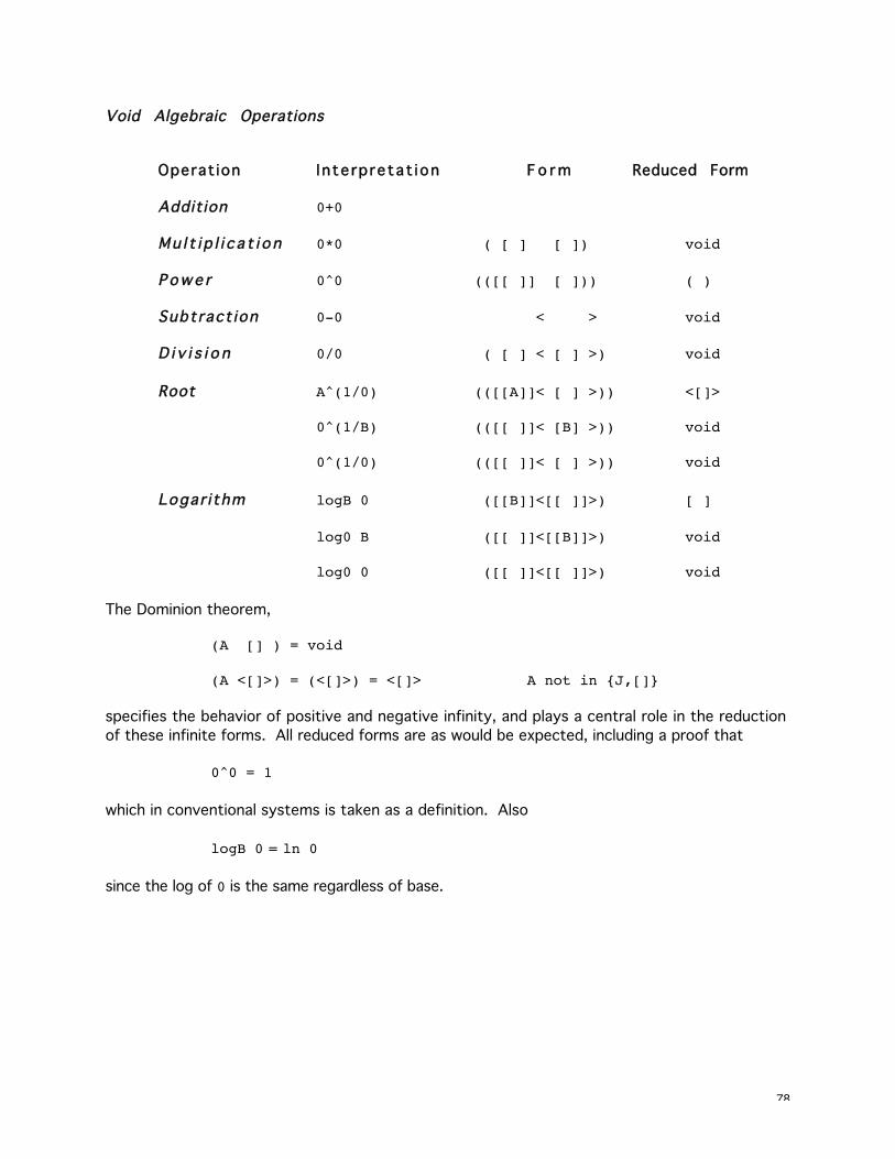
78

Void Algebraic Operations

Operat ion Interpretat ion F o r m Reduced Form

Addition 0+0

Mu l t i p l i c a t i o n 0*0 ( [ ] [ ]) void

P o w e r 0^0 (([[ ]] [ ])) ( )

Subtract ion 0-0 < > void

D i v i s i o n 0/0 ( [ ] < [ ] >) void

Root A^(1/0) (([[A]]< [ ] >)) <[]>

0^(1/B) (([[ ]]< [B] >)) void

0^(1/0) (([[ ]]< [ ] >)) void

Logar i thm logB 0 ([[B]]<[[ ]]>) [ ]

log0 B ([[ ]]<[[B]]>) void

log0 0 ([[ ]]<[[ ]]>) void

The Dominion theorem,

(A [] ) = void

(A <[]>) = (<[]>) = <[]> A not in {J,[]}

specifies the behavior of positive and negative infinity, and plays a central role in the reduction

of these infinite forms. All reduced forms are as would be expected, including a proof that

0^0 = 1

which in conventional systems is taken as a definition. Also

logB 0 = ln 0

since the log of 0 is the same regardless of base.

79

Reduction proofs:

0^0 (([[]] []))( ) dominion

0/0 ([]<[]>) void dominion

0^(1/0) (([[]] < [] >))(([[]] )) infinite absorption

void involution

0^(1/B) ([[B]]< [[]] >)([[B]]< J <[]>>) loglog 0

([[B]]<<J><[]>>) J inverse

([[B]]<<J []>>) inverse collect

([[B]] J [] ) inverse cancel

( [] ) dominion

void involution

log0 0 ([[ ]]<[[ ]]>)(J [ ]<[[ ]]>) loglog 0

void dominion

Infinities and Contradiction

The James calculus has a natural representation of infinity, <[]> which can be used

computationally. However, the use of infinity leads to contradictions, just as it does in standard

approaches. Fortunately, these contradictions can be eliminated by restricting specific

transformation rules.

Division by Zero

An initial question concerns the form of division by zero. It is clear that

A/0 = inf ([A]<[]>)( <[]>) positive dominion

<[]> inf

But what is 0 divided by 0?

0/0 ([ ]<[]>)

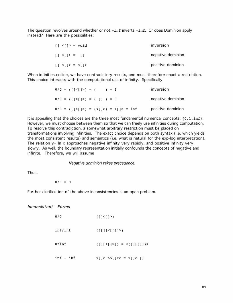
80

The question revolves around whether or not +inf inverts -inf. Or does Dominion apply

instead? Here are the possibilities:

[] <[]> = void inversion

[] <[]> = [] negative dominion

[] <[]> = <[]> positive dominion

When infinities collide, we have contradictory results, and must therefore enact a restriction.

This choice interacts with the computational use of infinity. Specifically

0/0 = ([]<[]>) = ( ) = 1 inversion

0/0 = ([]<[]>) = ( [] ) = 0 negative dominion

0/0 = ([]<[]>) = (<[]>) = <[]> = inf positive dominion

It is appealing that the choices are the three most fundamental numerical concepts, {0,1,inf}.

However, we must choose between them so that we can freely use infinities during computation.

To resolve this contradiction, a somewhat arbitrary restriction must be placed on

transformations involving infinities. The exact choice depends on both syntax (i.e. which yields

the most consistent results) and semantics (i.e. what is natural for the exp-log interpretation).

The relation y= ln x approaches negative infinity very rapidly, and positive infinity very

slowly. As well, the boundary representation initially confounds the concepts of negative and

infinite. Therefore, we will assume

Negative dominion takes precedence.

Thus,

0/0 = 0

Further clarification of the above inconsistencies is an open problem.

Inconsistent Forms

0/0 ([]<[]>)

inf/inf ([[]]<[[]]>)

0*inf ([][<[]>]) = <([][[]])>

inf - inf <[]> <<[]>> = <[]> []

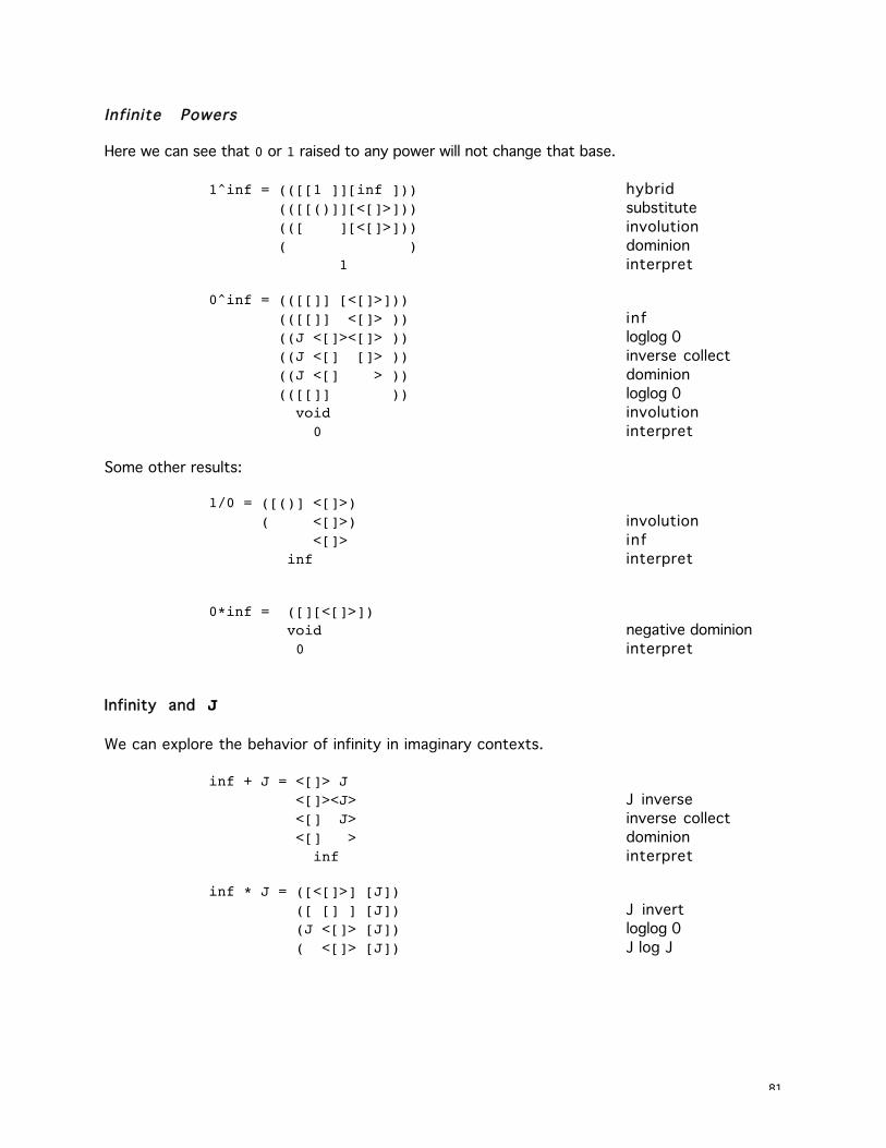
81

Infinite Powers

Here we can see that 0 or 1 raised to any power will not change that base.

1^inf = (([[1 ]][inf ])) hybrid

(([[()]][<[]>])) substitute

(([ ][<[]>])) involution

( ) dominion

1 interpret

0^inf = (([[]] [<[]>])) (([[]] <[]> )) inf

((J <[]><[]> )) loglog 0

((J <[] []> )) inverse collect

((J <[] > )) dominion

(([[]] )) loglog 0

void involution

0 interpret

Some other results:

1/0 = ([()] <[]>)( <[]>) involution

<[]> inf

inf interpret

0*inf = ([][<[]>]) void negative dominion

0 interpret

Infinity and J

We can explore the behavior of infinity in imaginary contexts.

inf + J = <[]> J <[]><J> J inverse

<[] J> inverse collect

<[] > dominion

inf interpret

inf * J = ([<[]>] [J]) ([ [] ] [J]) J invert

(J <[]> [J]) loglog 0

( <[]> [J]) J log J

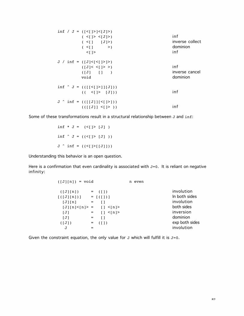
82

inf / J = ([<[]>]<[J]>) ( <[]> <[J]>) inf

( <[] [J]>) inverse collect

( <[] >) dominion

<[]> inf

J / inf = ([J]<[<[]>]>) ([J]< <[]> >) inf

([J] [] ) inverse cancel

void dominion

inf ^ J = (([[<[]>]][J])) (( <[]> [J])) inf

J ^ inf = (([[J]][<[]>])) (([[J]] <[]> )) inf

Some of these transformations result in a structural relationship between J and inf:

inf * J = (<[]> [J] )

inf ^ J = ((<[]> [J] ))

J ^ inf = ((<[]>[[J]]))

Understanding this behavior is an open question.

Here is a confirmation that even cardinality is associated with J=0. It is reliant on negative

infinity:

([J][n]) = void n even

([J][n]) = ([]) involution

[([J][n])] = [([])] ln both sides

[J][n] = [] involution

[J][n]<[n]> = [] <[n]> both sides

[J] = [] <[n]> inversion

[J] = [] dominion

([J]) = ([]) exp both sides

J = involution

Given the constraint equation, the only value for J which will fulfill it is J=0.

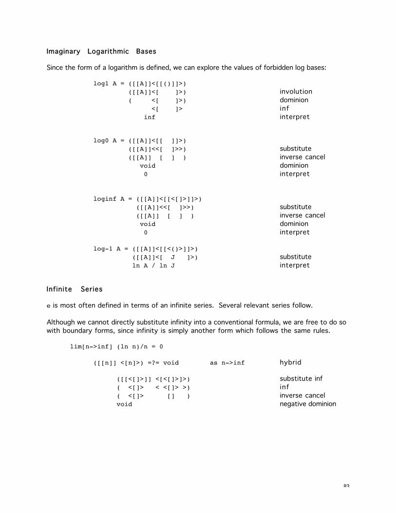
83

Imaginary Logarithmic Bases

Since the form of a logarithm is defined, we can explore the values of forbidden log bases:

log1 A = ([[A]]<[[()]]>) ([[A]]<[ ]>) involution

( <[ ]>) dominion

<[ ]> inf

inf interpret

log0 A = ([[A]]<[[ ]]>) ([[A]]<<[ ]>>) substitute

([[A]] [ ] ) inverse cancel

void dominion

0 interpret

loginf A = ([[A]]<[[<[]>]]>) ([[A]]<<[ ]>>) substitute

([[A]] [ ] ) inverse cancel

void dominion

0 interpret

log-1 A = ([[A]]<[[<()>]]>) ([[A]]<[ J ]>) substitute

ln A / ln J interpret

Infinite Series

e is most often defined in terms of an infinite series. Several relevant series follow.

Although we cannot directly substitute infinity into a conventional formula, we are free to do so

with boundary forms, since infinity is simply another form which follows the same rules.

lim[n->inf] (ln n)/n = 0

([[n]] <[n]>) =?= void as n->inf hybrid

([[<[]>]] <[<[]>]>) substitute inf

( <[]> < <[]> >) inf

( <[]> [] ) inverse cancel

void negative dominion

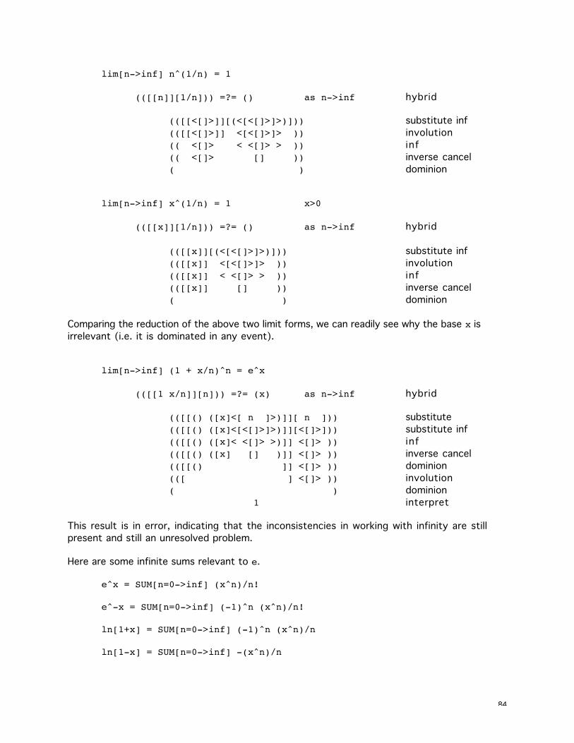
84

lim[n->inf] n^(1/n) = 1

(([[n]][1/n])) =?= () as n->inf hybrid

(([[<[]>]][(<[<[]>]>)])) substitute inf

(([[<[]>]] <[<[]>]> )) involution

(( <[]> < <[]> > )) inf

(( <[]> [] )) inverse cancel

( ) dominion

lim[n->inf] x^(1/n) = 1 x>0

(([[x]][1/n])) =?= () as n->inf hybrid

(([[x]][(<[<[]>]>)])) substitute inf

(([[x]] <[<[]>]> )) involution

(([[x]] < <[]> > )) inf

(([[x]] [] )) inverse cancel

( ) dominion

Comparing the reduction of the above two limit forms, we can readily see why the base x is

irrelevant (i.e. it is dominated in any event).

lim[n->inf] (1 + x/n)^n = e^x

(([[1 x/n]][n])) =?= (x) as n->inf hybrid

(([[() ([x]<[ n ]>)]][ n ])) substitute

(([[() ([x]<[<[]>]>)]][<[]>])) substitute inf

(([[() ([x]< <[]> >)]] <[]> )) inf

(([[() ([x] [] )]] <[]> )) inverse cancel

(([[() ]] <[]> )) dominion

(([ ] <[]> )) involution

( ) dominion

1 interpret

This result is in error, indicating that the inconsistencies in working with infinity are still

present and still an unresolved problem.

Here are some infinite sums relevant to e.

e^x = SUM[n=0->inf] (x^n)/n!

e^-x = SUM[n=0->inf] (-1)^n (x^n)/n!

ln[1+x] = SUM[n=0->inf] (-1)^n (x^n)/n

ln[1-x] = SUM[n=0->inf] -(x^n)/n

85

Working with James calculus and infinite series is an open problem.

D i f fe rent iat ion

Let 'A' be dA. The rules of differentiation in the James calculus expressed as are:

Name De r i va t i ve Interpretat ion

constant 'c' = void dc = 0

x/dx 'x' = () dx = 1

exponent '(A)' = ( A ['A']) de^A = e^A dA

logarithm '[A]' = (<[A]>['A']) dln A = 1/A dA

inverse '<A>' = <'A'> d-A = -dA

space 'A B' = 'A' 'B' d(A+B) = dA + dB

These rules are syntactically very regular, and thus useful for algorithmic computation.

Proof of the Chain Rule of Differential Calculus

d(AB) = B dA + A dB

'([A][B])'

([A][B]['[A][B]']) exponent

([A][B]['[A]''[B]']) space

([A][B][(<[A]>['A']) (<[B]>['B'])]) logarithm

([A][B][(<[A]>['A'])]) ([A][B][(<[B]>['B'])]) distribution

([A][B] <[A]>['A']) ([A][B] <[B]>['B'] ) involution

([B]['A']) ([A]['B']) inversion

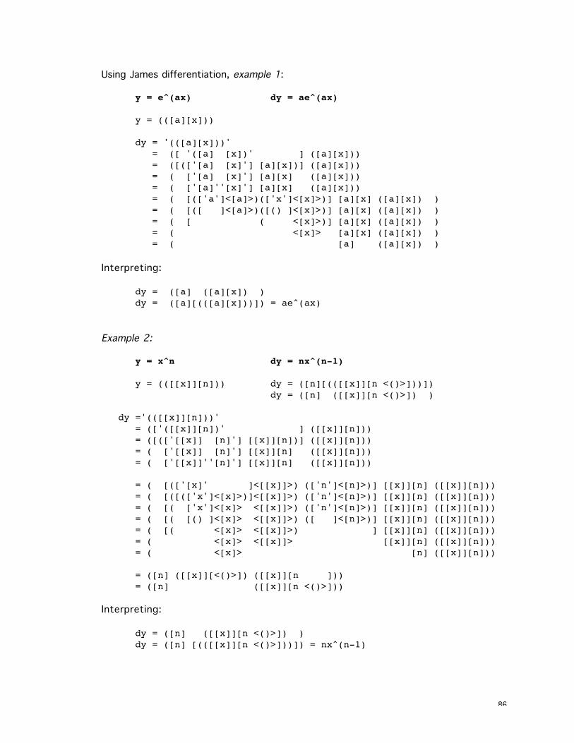
86

Using James differentiation, example 1:

y = e^(ax) dy = ae^(ax)

y = (([a][x]))

dy = '(([a][x]))' = ([ '([a] [x])' ] ([a][x])) = ([(['[a] [x]'] [a][x])] ([a][x])) = ( ['[a] [x]'] [a][x] ([a][x])) = ( ['[a]''[x]'] [a][x] ([a][x])) = ( [(['a']<[a]>)(['x']<[x]>)] [a][x] ([a][x]) ) = ( [([ ]<[a]>)([() ]<[x]>)] [a][x] ([a][x]) ) = ( [ ( <[x]>)] [a][x] ([a][x]) ) = ( <[x]> [a][x] ([a][x]) ) = ( [a] ([a][x]) )

Interpreting:

dy = ([a] ([a][x]) )dy = ([a][(([a][x]))]) = ae^(ax)

Example 2:

y = x^n dy = nx^(n-1)

y = (([[x]][n])) dy = ([n][(([[x]][n <()>]))])dy = ([n] ([[x]][n <()>]) )

dy ='(([[x]][n]))'= (['([[x]][n])' ] ([[x]][n]))= ([(['[[x]] [n]'] [[x]][n])] ([[x]][n]))= ( ['[[x]] [n]'] [[x]][n] ([[x]][n]))= ( ['[[x]]''[n]'] [[x]][n] ([[x]][n]))

= ( [(['[x]' ]<[[x]]>) (['n']<[n]>)] [[x]][n] ([[x]][n]))= ( [([(['x']<[x]>)]<[[x]]>) (['n']<[n]>)] [[x]][n] ([[x]][n]))= ( [( ['x']<[x]> <[[x]]>) (['n']<[n]>)] [[x]][n] ([[x]][n]))= ( [( [() ]<[x]> <[[x]]>) ([ ]<[n]>)] [[x]][n] ([[x]][n]))= ( [( <[x]> <[[x]]>) ] [[x]][n] ([[x]][n]))= ( <[x]> <[[x]]> [[x]][n] ([[x]][n]))= ( <[x]> [n] ([[x]][n]))

= ([n] ([[x]][<()>]) ([[x]][n ]))= ([n] ([[x]][n <()>]))

Interpreting:

dy = ([n] ([[x]][n <()>]) )dy = ([n] [(([[x]][n <()>]))]) = nx^(n-1)

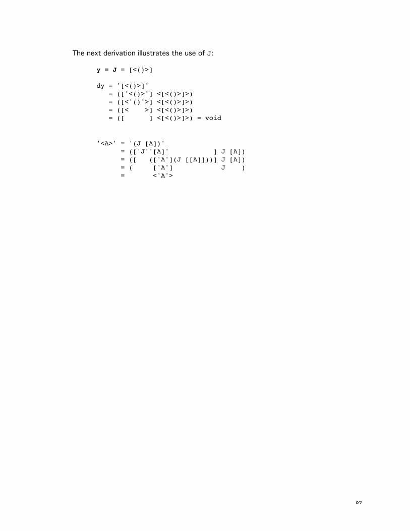
87

The next derivation illustrates the use of J:

y = J = [<()>]

dy = '[<()>]' = (['<()>'] <[<()>]>) = ([<'()'>] <[<()>]>) = ([< >] <[<()>]>) = ([ ] <[<()>]>) = void

'<A>' = '(J [A])'= (['J''[A]' ] J [A])= ([ (['A'](J [[A]]))] J [A])= ( ['A'] J )= <'A'>

Boundary Number Systems Table of Contents Boundary Number Systems William Bricken January 2001 Table...

Documents

Transcript of Boundary Number Systems Table of Contents Boundary Number Systems William Bricken January 2001 Table...