TICAM REPORT 96-26June 1996·

Boundary-Hybrid Finite Elements and A PosterioriError Estimation

Joseph M Maubach and Patrick J. Rabier

BOUNDARY-HYBRID FINITE ELEMENTS

AND A POSTERIORI ERROR ESTIMATION

BY

JOSEPH M. MAUBACH

AND

PATRICK J. RABIER

Department of Mathematics

University of Pittsburgh

Pittsburgh, PA 15260

ABSTRACT. Finite element methods that calculate the normal derivat.ive of the solution along

the mesh interfaces and recover the solution via local Neumann problems were introduced

about two decades ago by 1. Babuska, J.T. Oden and J.K. Lee for the treatment of the homo-

geneous Laplace equation and called "boundary-hybrid method". We revisit this approach for

general symmetric and positive definite elliptic equations with homogeneous boundary condi-

tions. The resulting approximation is nonconforming, and the corresponding error is orthog-

onal to all the conforming finite element subspaces. This crucial property shows immediately

how to derive an a posteriori error estimator for conforming finite element approximations via

Pythagoras' theorem. The investigation of this idea leads to a sound strategy for a posteriori

error analysis which gives conservative, yet accurate, estimates, is cheap for good conforming

approximations, and otherwise produces an enhanced solution at not significantly more than

the cost normally expected for such a result.

1. Introd uction.

In the second part of their paper "Mixed-Hybrid Finite Element Approximations of

Second-Order Elliptic Boundary Value Problems", Babuska, Oden and Lee [3], [4] discuss

e-mail: joseph@garfield.math.pitt.edu

rabier@vms.cis.pitt.edu .

1

an original finite element procedure, coined as "boundary hybrid method", to solve the

homogeneous Laplace equation

(1.1) {

6.u = 0

u=g

in n,on an,

where n c JR2 is a polygonal domain. Roughly, the procedure can be described as follows:

Consider a partition P of the domain n into polygonal elements. If the normal derivative

au / av of the solution is known across all the element interfaces, then the solution u can

(obviously) be recovered by solving the corresponding Neumann problem for the homoge-

neous Laplace equation over each element separately. A variational characterization of the

normal derivative au/ av is obtained in [4, Theorem 3.3]. Then, approximations of au / av,

e.g. by functions which are polynomials in each interface can be found by restricting

the variational formulation to an appropriate finite-dimensional space (standard Galerkin

procedure). To obtain u numerically, it suffices to solve the Neumann problem over each

element with auf av being replaced by its piecewise polynomial approximation. Of course,

the local Neumann problems need not be solved exactly, and in [4] this is exploited by

using higher degree harmonic polynomials within each element.

The specific form of the system (1.1) may have seemed especially important in light of

the fact that essentially no other elliptic problem has such an easily characterized dense

subset of solutions as the harmonic polynomials in two variables (a basis obtains by taking

the real and imaginary parts of (x + iy)n,n EN). However, with the advent of parallel

machines, any system of independent local problems can now be solved numerically at low

cost and with high accuracy and execution speed. Thus, the explicit knowledge of a special

set of solutions is no longer of significant help or importance.

In this paper, we give a variational characterization of the normal derivative of the

solution along element interfaces for general (symmetric) elliptic problems of the form

(1.2) {

- \7. A\7u + (J'U = f in n,u = 0 on an,

where D is an open bounded subset of JRn and f E L2(D). Here, "normal derivative"

must be understood as "A-normal derivative", i.e. au/avA := A\7u . v. Naturally, it is of

2

importance that the quadratic form used for the characterization of au javA satisfies basic

properties of continuity and coercivity. In practice, this means that adequate care should

be given to the definition of its domain.

One available option is to use the characterization of auj avA towards the numerical

approximation of u, as was done in [4]for the problem (1.1). However, a fuller application

can be found to the a posteriori estimation of u - it when it E HJ (.0) is any approximation

of u. It is this second and less standard aspect that we have chosen to emphasize here.

vYithout going into technicalities, the general idea is to partition the domain n into

nonoverlap ping subdomains nJ( whose boundaries relative n (i.e. not including f := an)constitute the interface set fI. Denoting by A the space L2(fI), a first step consists in

constructing a suitable completion A of A (not surprisingly of H-1/2 type). The completion

A is problem-independent. Assumptions are made which ensure that the symmetric bilinear

form a(-,·) in HJ(n) associated with (1.2) is coercive. Given it E HJ(n), a it-dependent

quadratic form Q in A is constructed with the crucial property that

(1.3) a( u - it, u - it) = in[Q(-\),..\EA

and that the unique minimizer l of Q corresponds canonically to the A-normal derivative

of aujavA along the interface fI.

It turns out that the fact that l depends only upon u (i.e. not upon it) is of importance,

for after discretization of the space A, a minimization procedure of Q can be started with

a it-related initial guess -\0. If it is a good approximation of u, then Q(-\o) is expected to

fall below some prescribed tolerance T chosen to assess the quality of the approximation

it. If so, (1.3) shows that a(u - it,u - it) :::; T, and it is called a good approximation.

Otherwise, the minimization of Q(-\) by an iterative procedure produces a minimizing

sequence -\j,j ~ O. Once again from (1.3), it is called a good approximation if Q(Aj) ~ T

for some j, and the minimization procedure may stop. If, on the other hand, Q( Aj) > T

until the minimization procedure is complete, then it is (conservatively) deemed to be a

poor approximation. This means that a new approximate solution must be determined.

Remarkably, this can be accomplished with no further work, because the minimization of

3

Q, now complete, also provides an enhanced solution if the discretization of the space A

has been properly chosen in the first place. This enhanced solution is not in HJ(n), as it

exhibits discontinuities along fI, but this is easily remedied if desired.

In summary, the error estimator described here has the two desirable features of always

providing an overestimate of the actual energy norm error and of yielding an enhanced

solution if the given approximation is not satisfactory. Furthermore, the workload IS,

loosely speaking, "inverse" proportional to the quality of the approximation.

All the numerical aspects involved in the minimization of Q are at least competitive

with those of traditional finite element methods (sparsity, size, storage, condition number,

etc ...). Of course, the fact that the domain of Q consists offunctions defined in the interface

f I is essential regarding size and storage: For instance, if n = 2 and discretization of A

is made via piecewise polynomials of degree k, the size of the system grows linearly with

respect to k instead of quadratically when a standard finite element method is used. Yet,

as we shall see, the latter do not produce more accurate solutions. Static condensation

reduces the problem to one of the same size as ours, but still requires much more storage

than our method for large k.

The local problems need to be solved just once at the beginning of the procedure and

not at each iteration as could be inferred from our initial comments. Not only this step

is evidently fully parallelizable, but even the minimization of Q lends itself perfectly to

elementwise parallel processing by the method recently introduced in [9] and [10].

Section 2 is devoted to some preliminaries including a definition of a space A_ which,

later (Section 4), will be shown "canonically" isomorphic to the space A mentioned earlier.

There are some notational technicalities due to the fact that normal derivatives along

sub domain interfaces are, of necessity, double-valued with one value being the negative

of the other. Our presentation bypasses the explicit use of oriented integrals (to avoid

mixing oriented and nonoriented integrals, and because no convenient symbol such as f is

standard in dimension greater than one) but this is a matter of taste and not a conceptual

difference.

In Section 3, we present the variational characterization of the A-normal derivative

along the interface fI and describe the error related to the discretization and Galerkin

4

approximation. It is also shown that the estimator yields justifiable local error indicators,

although the upper bound property is lost at the local level.

Section 5 addresses the important issue of the accuracy of the error estimator in a

somewhat restricted setting nevertheless sufficient for most two-dimensional applications.

The results of Section 5 have the form of a priori estimates and show that both the error

estimator and the enhanced solution have optimal orders of accuracy. No "saturation

assumption" ([1], [6]) is needed. In addition, an unusual feature is highlighted: If the

partitioning of the open subset n is done according to a simple rule, the accuracy depends

only upon the interior regularity of the solution u and not upon its global regularity (the

latter being always limited by the presence of corners in .0).

When (7 = 0 in (1.2), the minimization of Q involves a linear constraint (more generally,

the same thing is true whenever (7 vanishes in a set with positive measure). The slight

modifications to the procedure needed in that case al'e examined in Section 6.

Section 7 presents numerical experiments.

2. Notation and preliminaries.

Let n c ]Rn be a bounded open subset with Lipschitz continuous boundary f. We

shall consider a "partition" P of n into open sub domains nK,l :::;J{ :::;N, satisfying a

number of technical conditions. These conditions always hold when P is built from a finite

element triangulation of n and the nK's are the elements or patches of elements of the

triangulation.

Specifically, we require thatN _ _

(H1) u .oK = n.K=I

(H2) .oK n nL = 0 if J{ #- L.

(H3) The boundary f K := anK is Lipschitz continuous.

It follows from (H3) that the n-dimensional Lebesgue measure of rK is zero, whence,

from (H1) and (H2):

(2.1)

5

where all the integrals must be understood in the sense of the n-dimensional Lebesgue

measure.

It also follows from (H3) that the boundary f K may be equipped with a "canonical"

Lebesgue measure, denoted by µK. For 0:::; ](,L :::;N, set fo := f and

(2.2)

Cleary, fKL is a closed subset of both fK and fL, and hence fKL is both µl(- and µL-

measurable. As a result, fl(L may be equipped with both µK and µL measures. A natural

requirement now is

(H4) µl(lr = µLlr 'KL KL

and then (H4) appears as a compatibility condition for the set

(2.3) - Nf:= U fI<

/(=0

to be equipped with a measure µ defined by the condition

(2.4)

Since f I< is Lipschitz continuous, an outward unit normal vector VK exists µK- a.e.

(that is, µ- a.e.) in fl(. As a result of (2.4) and (H4), both VI< and VL exist µ- a.e. III

rl( L, and we shall require that

(H5) {1 ~ ](, L :::;N,]( =I- L} :::}VI<I = -VL1 .rKL rKL

If fKLM := fK n fL n fM, it follows at once from (H5) that VM = 0 in f/(LM if

1 ~ ](, L, J.V1 :::; Nand ](, Land M are distinct. Since VM is a unit vector µ- a.e. this

implies that µ(f K LM) = 0 in this case. Our next assumption is that this also holds when

either K, L or J.V1is 0, i.e. that

(H6) {O::;](, L, J.V1:::;N, J{ =I- L, J{ =I- lvI, L =I- J.V1} :::} µ(f K n f L n f M) = o.Finally, we shall assume that for 0 ~ J{ ::; N,

N(H7) fK = U fKL.

L=OL~I<

6

Remark 2.1: It is not difficult to convince oneself that the hypotheses (H1) through (H7)

are not independent. We have not bothered with trying to find a minimal set of conditions

equivalent to (H1) - (H7) since the direct verification of (H1) - (H7) will never be an issue

in the applications we have in mind. 0

Let

(2.5) I:= {(K,L): 1:::; K,L:::; N,K # L,µ(fKL) > O},

and, for 1 :::;K :::;N,

(2.6) IK := {1 :::;L :::;N : (K,L) E I}.

Clearly, I is an index set for the interfaces f [(L, each being counted twice (once in f K

and once in f L), whereas IK labels (once) the interfaces contained in rK.

From (H6) and (H7), we have for 1 :::;K :::;N:

where the integrals are understood in the sense of the measure µ. Obviously, the integrals

corresponding to pairs (K, L) with µ(f]( L) = 0 in the right-hand side may be discarded,

so that

(2.7)

In (2.7), the term fr disappears whenever µ(fKo) = O.J1 1<0

Let fI be the disjoint union

I'I:= II fI<L,(K,L)EI

so that, in fI,fKL and fLK are different although they coincide as subsets of ]Rn. Ac-

cordingly, we set

7

Elements of L2(rI) thus are collections ~ = (AKL) with AKL E L2(fKL). In general, the

functions AKL and ALK are different, despite the fact that they are both defined in the

same subset f K L of IRn.

There is a canonical identification

(2.8)N

L2(rI) ~ IIL2(f K \ f),K=l

obtained by associating with ~ = (AKL) E L2(rI) the collection (AK) defined by AKIr[(L

AKL,L E IK (this makes sense because of (H6),and AK is defined µ- a.e. in fK becauseN _

of (H7». The inverse map is given by (AK) E II L2(fK \ f) t---+ (AKL) E L2(fI) whereK=l

AKL := AK, .rKL

In future considerations, it will be convenient to use both the notations (AI<£) and

(AK) for elements of L2(rI) (depending upon whether the identification (2.8) is used).

No confusion should arise from this since the number of subscripts immediately identifies

which definition of L2(rI) is being used.

The norm of L2(I'I) is the natural one, namely

(2.9)

\Ve shall consider the spaces

(2.10)

with norm induced by t.he norm of HI(nl(), and the products

(2.11)N

HJ(P) := II VK,[(=1

N

HI(p) := II H1(nK)K=l

equipped with the product norm 1I·lh;p. Evidently, in (2.10) we have VK = HI(nK) when

µ(rKO) = o.

8

A restriction map (trace) is defined:

(2.12)

which is of course linear and continuous for the norms of the spaces involved. On the other

hand, there are canonical embeddings

(2.13)

defined by v E HI (.0) ~ (VloK

)' Our first result gives a simple characterization of the

image of the embedding (2.13) via the trace operator (2.12) and the closed subspace of

L2(fI ):

(2.14)

Proposition 2.1. Let (VK) E H1 (P) and let v E L2(n) be defined by VIOK := VI(. Then,

v E H1(n) if and only if (VKI ) E A+ (where the identification (2.8) was used).rK\r

Proof. Ifv E COO(n) and VK:= vlo , it is obvious that VKI = VLI ' i.e. (VI(I ) EK rKL rKL rK\r

A+. By the denseness of COO(n) in H1(n), the continuity of the trace HI(P) --+ L2(fI)

and the closedness of A+ in L2(fI), this relation remains valid for v E HI(n).

Conversely, if (VI() E HI (P), V E L2(n) c 'D'(n) is defined by vloK

:= VI( and'P E'D(n),

we have

Since 'P = 0 in f, we find (see (2.7)

9

and the terms in the right-hand side cancel out if (VI<I ) E A+ (i.e. VK = VKL in fgL)r[(\r

since VKi = -VLi in f 1';L from (H5). It follows that

I.e. avjfJxi is represented by the L2(n) function defined by aVI<jaxi in nK, 1 :::;J{ :::;N.

Thus, V E H1(n). 0

The natural complement of the space A+ in (2.14), that is

(2.15)

plays a crucial role in our subsequent considerations. The starting point is the remark that

every element A = (AK) E A_ (where the identification (2.8) was used) can be viewed as

an element of

(2.16)

(see (2.10) and (2.11) via

(2.17)

K

H-1(P) := (HJ(P»* = IIV;K=I

The (product) norm of H-1(P) will be denoted by II . II-l,P.If wE HJ(n), then w can be identified with the collection (wln[() E HJ(P) through the

embedding (2.13), so that (~, w) makes sense. Note that

(2.18)

because

- 1(A, w) = 0, Vw E Ho (n), VA E A_,

Nj j~ AK'wK = ~ AKwK,K=I r[(\r (K,L)EI r[(L

and all the terms in the right-hand side cancel out since 10 [( = w L in f K L (Proposition

2.1) whereas AI( = -)..L in f[{L if ~ E A_.

10

Definition 2.1. The space A_ is the closure of A_ in H-I (P).

From Definition 2.1, every .:\ E A- is the limit in H-1(P) of a sequence from the space

A_. From (2.18) we obtain by continuity that

(2.19) (.:\,w) = 0, Vw E HJ(n), VA E A_.

(2.20)

equipped with the norm

(2.21)

Naturally, similar definitions can be made for the spaces HA(flK), 1:::; J(:::; N.

If VK E CCXJ(D.K), we may define the "A-normal" derivative

(2.22)

Proposition 2.2. (i) The mapping v E CCXJ(nK) ~ aVKjavt E L2(fK) has a unique

linear continuous extension from HA(nK) into V!(. Furthermore, Green's formula

(2.23)

holds for WK E VK.

(ii) Ifv E cCXJ(n) and VK:= vloK

' 1 ~ J(::; N, then the collection (avKjaVj~) can be

viewed as an element of H-1(P) via

(2.24) (aVK) N 1 aUK( av~ ' (WI(») := K~l a A WI(, V(WI() E HJ(P),!\ fJ( VI(

11

and, in H-I(P), we have (avKlav~) E A_.

(iii) The mapping v E c=(n) -- (aVI\-!avt) E A_ C H-1(P) (where VK := vloK

) has

a unique linear continuous extension from H.4.(n) into A_ C H-1(P).

Proof. (i) This is essentially standard. Briefly, for VK E COO(nK) and by Green's formula,

we have

(2.25)

for WK E COO(nK), and hence for WK E H1(ng). In particular, (2.25) holds for WK E VK,

and it follows that

where AI, > 0 is a constant depending only upon .4,. As a result,

(2.26)

with II· IIr n denoting the norm of VI(.,K

The existence and uniqueness of a continuous extension of av K I avt as an element of

V'/( for VK E HA(nK) follows from (2.26) and the denseness of COO(n/\,) in HA(D.g). (For

the latter point, see Grisvard [8, p. 59] when .-l = I; the proof in the general case is

similar.) Next, (2.23) is just the extension of (2.25) by denseness and continuity.

(ii) The only point to be emphasized here is that, as an element of H-1(P), we have

((avKlav~» E A_. This follows from the fact that for (wg) E HJ(P), we have

I.e. ((aug I av~» and ((av/( I Bvt »lrK\r) coincide in H-1 (P), while aVI{ I av~ = -BVLI avt

in rKL,(K,L) E I, from (H5) and from \7v/( = \7vL = \7v in rKL when v E COO(n).

12

N(iii) First, from (ii), the mapping v E c=(n) t-+ ((aV[(jav~» E IT L2(fK) has

K=lN

a unique linear continuous extension from HA(n) into IT V; := H-I(P). From (ii),K=l

(avKjaV~) E A_ when v E c=(n), and by using once again the denseness of c=(n) in

HA(n) it follows that (avKjaVp:> E A_. 0

Remark 2.2: Part (i) of Proposition 2.2 remains valid with VK replaced by HI (nK), andN

(2.17) also defines an embedding of A_ into IT HI(nK)*. Although (avKjaV~) can beK=I

Nviewed as an element of IT HI(nK)* via (2.24), it is not true that (aVK j av~) E A_ in

K=Ithis case, because the integrals in the right-hand side of (2.24) do not reduce to integral

Nin f K \ f. It follows that for v E HA(n), (aVl( j av~) E IT H1(nK)* cannot be viewed as

K=lN

an element of the closure of A_ in IT H1(ng)*. 01(=1

3. Application to a posteriori error estimation.

From now on, we assume that the matrix A. = (aij) E (C1(n»nxn is symmetric (aij =aji) and satisfies the uniform ellipticity condition

(3.1)

where a > 0 is a constant and 1·1 denote the euclidian norm. Given a function (7 E L=(n)

such that

(3.2) (7( x) ~ 0'0 > 0 a.e. in .0,

and a function f E L2(n), we consider the boundary value problem

(3.3) {

- \7. (AY'u) + (7U = f in n,u = 0 in r,

whose (unique) solution u E HJ(n) is characterized by

(3.4) a(u,v) = in fv, V v E HJ(n),

13

where a(·, .) : HJ (.0) x HJ( n) -+ ]R is the bilinear symmetric form

(3.5) a(v,w):= in(A\7v)' \7w + in (7VW.

For 1 :::;J( :::; N, we consider the "sub domain" bilinear forms a!\-(·,·) : VI\" X VI\" -+ ]R

defined by

(3.6)

and their sum ap(-,') : HJ(P) x HJ(P) -+ ]R

(3.7)

Ifv,w E HJ(n) and VI(:= VlnK,WI(:= WinK' SO that v = (VI() and W = (WI() modulo

the embedding (2.13), then

(3.8)

by (2.1), (3.5) and (3.7).

ap(v,w) = a(v,w), V V,W E HJ(f2)

The bilinear forms aI«(·,·) are now used to solve "local" Neumann problems:

Lemma 3.1. Let ~ := (AI() ElL, so that AI( E V!(, 1 :::;J{ :::;N. Then, there is a unique

element ¢>(A):= (¢>I«(AI\"» E HJ(P) such that

(3.9)

In addition, there are constants C1 (P) > 0 and C2(P) > 0 independent of A such that

(3.10)

Proof. By (3.1) and (3.2) the bilinear forms aJ«(·,·) are VI(- coercive, whence the existence

and uniqueness of ¢>I«(AI(). The inequalities in (3.10) follow at once from the properties

14

It follows that if> K(>..K) in (3.9) can be viewed, formally at

of A and (7 und the definition of the norms of H6(P) and H-1 (P) through standard

elementary arguments. 0

Fix 1 :::;1(0 :::;N and let v E V(nKo), so that v](o = v, v]( = 0 for K # Ko. By (2.19),

()'Ko,VKo) = 0 if ~ = (AK) E A_. This shows that for general VKo E VKo, (AKo,VKo)

depends only upon V](oIrKo

least, as the solution of the boundary value problem

¢K(AK) = 0 in fl( n f,

a¢J«(AJ()javt = AK in f \ fJ(.

Lemma 3.2. Let ~ E A_ and let ¢(~) E HJ(P) be defined as in Lemma 3.1. Then

- 1ap(¢(A),V) = 0, \Iv E Ho(n).

Proof. Let ~ = (AJ(), so that ¢(~) = (¢]((>.J() and (3.9) holds. In particular, let v E

HJ(n) and set VJ( := vloK

' From (3.7) and (3.9), we have

_ N _

ap(¢(A),V) = ~ (AJ(,V]() = (A,v),1\=1

and (~, v) = 0 by (2.19). 0

Now, let it E H J (n) be an arbitrary element. In practice, it may be viewed as an

approximation of the solution u of (3.3) - (3.4). By the VJ(-ellipticity of the bilinear form

aJ«(·, .), we obtain

Lemma 3.3. There is a unique clement 13:= (13K) E HJ(P) such that

(3.11)

15

Lemma 3.4. Let ~ E A_, and let ¢(~), {3 E HJ(P) be defined as in Lemmas 3.1 and 3.3,

respectively. vVe have

(3.12)

and hence

(3.13)

a1'(¢(~) + {3,v) = a(u - it, v), '<IvE Hci(n),

a1'(¢(~) + {3 - (u - tt),v) = 0, '<IvE Hci(n).

Proof. From Lemma 3.2, we already have a1'(¢(~),v) = 0 for A E A_, so that (3.12)

amounts to

a1'({3,v) = a(u - it, v), '<IvE Hci(n).

To see this, add up the identities (3.11) with VK := vlOK

to get

and a1'(it,v) = a(it,v) by (3.8), fnfv = a(u,v) by (3.4). Relation (3.13) follows from

(3.12) since a(u - it,v) = a1'(u - it,v) by (3.8). 0

To motivate our next result, recall the canonical embedding (2.13): HJ (n) '--+ HJ(P).

Let ~ E A_ and suppose that ¢(~) + {3 E HJ(n) (and not merely HJ(P». Then, by (3.8)

and (3.12) and the HJ(n)-ellipticity of the bilinear form a(·,·) it follows t.hat ¢(~) + {3 =

u - it. Lemma 3.5 below shows that this happens for one and only one A E A_.

Lemma 3.5. For A E A_, the following conditions are equivalent:

(i) ¢(~) + {3 E HJ(n) (hence ¢(~) + {3 = u - it from the above).

(ii) ~ = (aUK jav~), where UK := U!OK' 1:::;]{ :::;N.

Proof. As a preamble, we note that (3.3) implies that u E H A(n), so that (aUK j f)Vj~) E A_by Proposition 2.2 (iii). Also, by Proposition 2.2 (i), we have

16

From (3.3), \7. (AVUK) = (7U[( - f, and hence the above formula may be rewritten as

Together with (3.9) and (3.11), this yields

(3.14)

(i) ~ (ii). If ¢C)..) + 13 = U - U, then (¢(5..) + (3)II1K = UK - uK· As (¢(5..) + (3)II1K

¢K(A[() + 13K (by definition of ¢(5..) and (3), it follows from (3.14) that (AK - aau!f, VK) =VK

0, VVK E VK. Thus, AK = aUKlavt in Vi<,l :::;J( :::;N, so that 5.. = X:= (auKlavt)N _ _

in n Vk = H-1(P) (hence A = l in A_ c H-1(P».K=I(ii) ~ (i). If 5.. = (auKlav~), then AK = aUKlavt is in Vk,l:::;]{:::; N, and (3.14)

reads

By the VK-ellipticity of aK(', .), this implies ¢K(AK) + 13K = uK - UK, 1 :::;]{ :::;N, and

hence ¢(A) + 13= U -u. 0

vVe are now in a position to give our main result, that is, a variational characterization

of X := (aUK Iavt)· This characterization permits the calculation of (aUK IaVR) without

any knowledge of the solution u. Instead, U - ti, and hence u, can next be obtained by

solving the local problems (3.9) and (3.11) with AK = aUK IaVI~'

Theorem 3.1. The quadratic functional J := A_ ~ IR defined by

(3.15) -- 1 - - -J(A) := "2ap(¢(A), ¢(A» + ap(f3, ¢(A),

is continuous and coercive, and its unique minimizer is X := (au K Iavt). In addition

(3.16)a( u - u, u - u) = 2J(X) + ap(f3, (3) :::; 2J( 5..) + ap(f3, (3) =

ap(¢(5..) + 13,¢(5..) + (3), VA E A_.

17

Proof. The continuity and coercivity of J are immediate consequences of the inequalities

(3.10). In order to prove that its unique minimizer is none other than X:= (auKjaVf{),

let us first observe that

(3.17)

Since u - it E HJ(n), we have ap(cP(~) + /3 - (u - it),u - it) = 0 for ~ E A_ by (3.13)

in Lemma 3.4. Thus, by writing cP(~) + (3 = cP(~) + (3 - (u - it) + (u - it), we infer that

(3.18)ap(cP(~) + (3, cP(~) + (3) =

ap(cP(~) + /3 - (u - it), cP(~) + /3 - (u - it» + ap(u - it,u - it),

for every A E A_.

Altogether, relations (3.17) and (3.18) show that 2J(~) + ap((3,/3) ~ ap(u - it,u - it),

with equality if and only if cP(~) + (3 = u - 'u, i.e. if and only if ~ = X from Lemma 3.5. In

summary, for A E A_, we have

2J(~) + ap(/3, (3) ~ 2J(X) + ap((3, (3) = ap( u - it, u - ,u).

This implies at once that

and that (3.16) holds since ap( u - it, u - it) = a( u - it, u - it) by (3.8). 0

From Theorem 3.1, the "energy-norm" error a( u - it, u - it )1/2 can be calculated via

the minimization of the functional J in (3.15). It is noteworthy that ~ E A_ is (loosely

speaking) defined only in I'I := II fKL, aset with dimension n-1. Also, the inequality(K,L)EI

(3.16) shows that the quantity

(3.19)

is always an overestimate of the actual error a( u - it, u - it )1/2. Thus, the discretization of- -

the space A_ and the use of approximate minimizers in place of l, two inevitable features

18

of any numerical minimization procedure, will produce conservative estimates of the actual

error.

A strategy for a posteriori error estimation: The most natural way to use (3.19)

as an error estimator is first to substitute for A data readily available from the approxi-

mate solution it itself. In practical applications when it is a (conforming) finite element

approximation, the derivative ait KIavt is always defined in the space L2 (f J( ), hence in

L2(fJ( \ r). However, in general (aitKlav~) ~ A_, whence ~ := (a'ClKlavt-) cannot be

chosen in (3.19). This is easily remedied, e.g. by choosing ~ = (AK) where

(3.20) VL E IK.

Incidentally, the choice (3.20) corresponds to ~ being the projection of (ait K Iavt) onto

A_ relative to the orthogonal splitting

(3.21)

Other weighted averages are suggested in Ainsworth and aden [1].

The step consisting in substituting ~ as given in (3.20) into (3.19) involves only solving

local problems (specifically, (3.9) and (3.11»), which can be done in parallel and with high

accuracy, yet at a nominal cost. If the estimator (3.19) falls below a prescribed tolerance,

(3.16) ensures that the energy norm a( u - it, u - 'u) 1/2 does not exceed that same tolerance,

and therefore it may be called a good approximation of u (relative, of course, to the given

tolerance) .

Otherwise, a finite-dimensional subspace A~ of A_ may be chosen in such a way that

~ in (3.20) satisfies the condition ~ E A~, and an iterative minimization procedure of

.J - or, equivalently, (3.19) - over A~ may be launched, with initial guess >'0 = >.. This

produces a sequence >.j E A~. If for any j ~1 the quantity a'P(fjJ(~j) + /3, fjJ(>.j) + /3)1/2

falls below the prescribed tolerance, the very same arguments used above when j = 0 show

that a( u - it, u - £t )1/2 does the same thing, hence it is a good approximation of u, and the

minimization procedure need not be continued further.

19

If the minimization of j over A~ arrives to completion, thus exhibiting a minimizer-kl E A~, the approximate solution it will be declared unsatisfactory (this is, of course,

a conservative call). Accordingly, a better solution should be sought. Here, a significant-k

bonus is that it +</J(~ ) +13, which obtains at no extra cost, is already an enhanced solution

if the space A~ has been chosen large enough. In this respect, see Remark 5.1 later and

subsequent comments. In other words, the effort for the minimization of j has not been

wasted. The enhanced solution it +</J(ik) +13 is not in HJ(n), being discontinuous across the

interfaces f KL. Thus, the error estimation procedure described above cannot be repeated-k

by simply replacing it by it + </J(l ) +13. But it should be clear that an HJ(n)-interpolation

of it + </J(ik) + 13 can be implemented at nominal cost, thus providing a slightly modified

approximation itl E HJ(n) of u whose quality can be tested again if desired.

The strategy outlined above relies upon Galerkin approximation. This aspect is dis-

cussed in more detail in the next section. In particular, it will be seen that local problems

need not be solved at each step: This can be done once and for all at the beginning of the

procedure for a set of (local) basis functions. It will also appear that the estimator has

justifiable value regarding local error estimation, an attractive feature in some applications.

Another important aspect is the accuracy of the estimator: The fact that any choice

of .\ E A_ in (3.19) produces an overestimate for a(u - it,u - it)1/2 was used in a crucial

way, but it is also important that the resulting estimator does not provide exceedingly

conservative predictions. This issue is considered in Section 5 in a special case relevant in

most (two-dimensional) problems. There, we will show that the estimator may be made

\'ery accurate (in theory, this depends upon the choice of the sub domains nK) for solutions

having good interior regularity.

4. Galerkin approximation.

Due to the fact that the elements of the space A_ correspond to two functions in each

interface f KL, (K, L) E I (one being the negative of the other), the spaces A_ and A_ are

somewhat inconvenient to use. Our first task here will be to reformulate the minimization

problem of Theorem 3.1 in a more familiar setting.

We shall denote by fI the interface ofthe partition P, that is, the (non disjoint; compare

20

with fI in Section 2) union

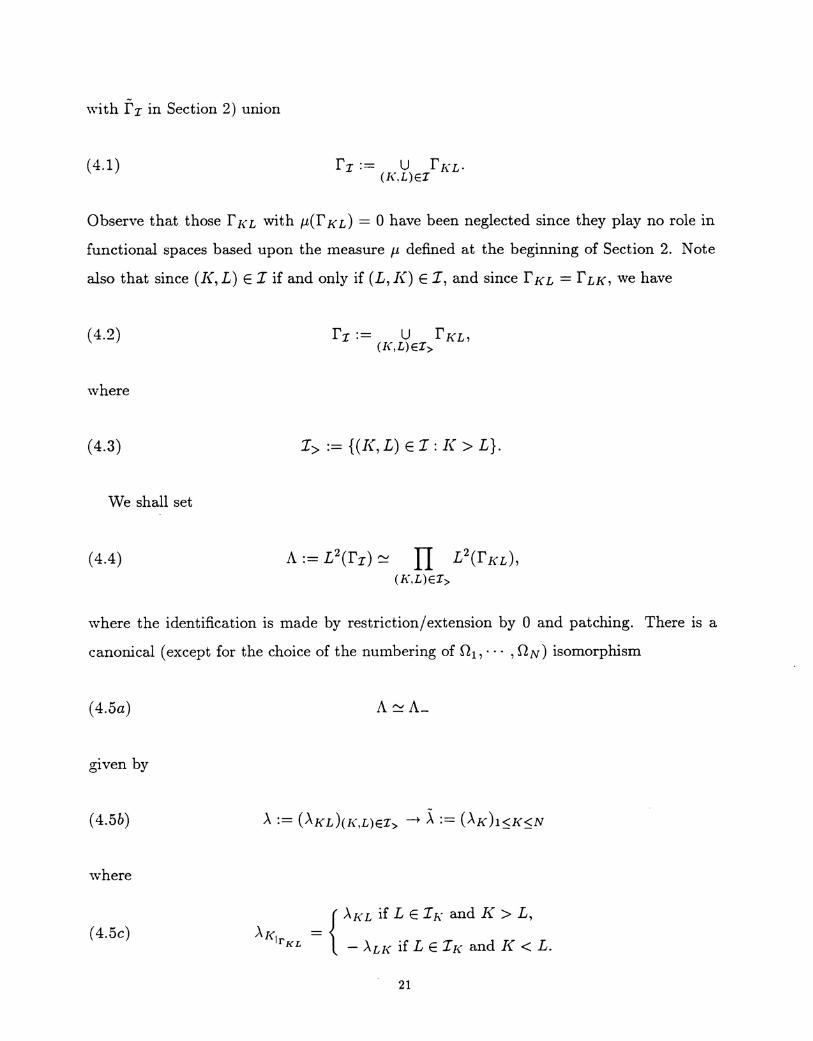
(4.1) fI := U fKL.(K,L)EI

Observe that those f K L with µ(f K d = 0 have been neglected since they play no role in

functional spaces based upon the measure µ defined at the beginning of Section 2. Note

also that since (K,L) E I if and only if (L,K) E I, and since fKL = fLK, we have

(4.2)

where

(4.3)

We shall set

(4.4)

fI:= U fKL,(K,L)EI>

I>:= {(K,L) E I: K > L}.

A := L2(fI) ~ IT L2(fKL),(K,L)EI>

where the identification is made by restrictionj extension by 0 and patching. There is a

canonical (except for the choice of the numbering of .01, ... , nN) isomorphism

(4.5a)

given by

(4.5b)

where

(4.5c) {

AKL if L EIK and K > L,AI( =

IrIa _ ALI( if L E If{ and K < L.

21

vVe shall denote by i\ the completion of the space A equipped with the H-l(P)-norm

"ia the isomorphism (4.5). It is then trivial that the isomorphism (4.5) extends as an iso-

morphism of A onto A_. For A E A, we shall denote by ~ the element of A_ corresponding

to A through this isomorphism.

As a result, the functional j in (3.15) becomes a functional

(4.6) - -- 1 - - -A E A ~ J(>.) := J(>.) := 2ap( 4>(A), 4>(>.» + ap( 4>(A), ,8),

which is continuous and coercive (Theorem 3.1). Also by Theorem 3.1, the unique mini-

mizer lEA of J is such that X = (auK j avt ).For each pair (K,L) E I>, let (A1LhEN be an increasing sequence of finite-dimensional

00

subspaces such that U A1<L is dense in L2 (f KL)' Call Ak the product spacek=O

(4.7) A k := II A j(L C A(K,L)EI>

(see (4.4». (The space A~ at the end of Section 3 is just the image of Ak through the

isomorphism (4.5).) Then, U Ak is dense in A (see (4.1» and hence in A since (obviously)k=O

A is dense in A. It thus follows from the continuity and coercivity of the functional

J in (4.6) along with general properties of the Galerkin approximation that the unique

minimizer lEA of J satisfies the condition

(4.8) \ l' \ k· A-~ = 1m ~ In ,k--oo

where for k E N,lk E Ak is the unique solution of the minimization problem

(4.9)

For A, B E A, we shall set

(4.10) b(>.,B):= ap(4)(~),4>(B))

22

and

(4.11)

so that

(4.12)

Given (K, L) E I>, set

(4.13)

f(A) := -ap(!3, 4>(~»

J(>') = ~b(A, A) - f(A), V >. E A.2

and let (pkL)l<i<dk be a basis of AtL' The functions p}(L can be viewed in A:= L2(fI)- - KL

after extension by 0 outside f K L, and then A E Ak C A has a unique decomposition

(4.14)

for suitable coefficients ekL E JR. As a result, the minimization of the functional J in

(4.12) amounts to solving a linear system

(4.15)

with symmetric positive definite matrix B with coefficients b(P}(L,P}J) and right-hand side

T] with components f(pkL)'

From (4.10) and (4.11), the calculation of the coefficients of B and of the components

of T] requires the calculation of the quantities 4>(P}(L)'

Fix (Ko, Lo) E I> and let 1 :::;i :::;dtLo' According to (3.9) (and recalling the defini-

tion of the embedding (4.5)), we have 4>(jj}(oLo) = (¢>K(P}(oLol )) where 4>K(P}(oLol

) =rK rK

o if K =1= Ko, K =1= Lo (because P}(oLo = 0 in fI \ fKoLo) and 4>Ko(pkoLolr

) andKo

4>Lo (pkoLo ) are characterized byIrLo

(4.16)

23

and

(4.17)

From the above, <P(P}(oLo) viewed as a function in L2(n), has support in nKo U nLo for

every (Ko,Lo) E I>. It now follows from (4.10) and the definition of the bilinear form

ap(·,·) (see (3.6) and (3.7» that if (K,L),(I,J) EI>:

unless (nK U nL) n (n[ u .oJ) i= 0 (i.e. I = K or L, or J = K or L). This result expresses

the sparsity of the matrix B.

It is also of some practical importance to notice that, after <p(p~J) has been determined,

the calculation of the coefficients b(pk L' p~J) reduces to an integral along f K L. Indeed,

we have by (4.10) and (3.6), (3.7) and (3.9)

But since PkL = 0 outside fKL, only the values M = K and AI = L are actually involved

in the right-hand side, and hence, recalling the embedding (4.5),

(4.18)

As the calculation of b(p}\oL' p}(L) requires using <p(p}( L)' all the <p(p}( d, (K, L) E I>, must

be determined. Since b(·, .) is symmetric, the roles of pk L and p~J can be exchanged in

(4.18) (which is not obvious from merely looking at the right-hand side).

The evaluation of the components of the right-hand side 1] of (4.15), i.e. of f(pkL) =-ap(j3, <p(pkd) (see (4.11» can be done as follows: First, j3 may be calculated via (3.11),

and next f(P}(L) is obtained through a boundary integral along fKL since, by (3.6), (3.7)

and (3.9) (and the symmetry of ape, .»

(4.19)

24

Remark 4.1: Since a1'((3,¢>(i>}\d) = fnf¢>(i>}(d - a1'(it,¢>(i>i\L» by (3.11), and since

<!>(P}(L) has support in D.K U D.L, we get (with (K,L) E I»

a formula showing that (3 need not be calculated at this stage. However, (3 is needed to

recover U - ii. = <p(~) + (3 and hence any approximation <p(.A) + (3 of u - U. 0

Local error estimation: It often happens that the quality of the approximation U of u is

not assessed solely by the smallness of a( u - u, U - U )1/2 but also depends upon the locally

defined quantities aK( UK - Ul(, UK - UK )1/2. It follows at once that the convergence of

<p(~k) + 13 towards u - U in energy norm implies

(4.21)

for every :fixed 1 :::;K :::;N. Therefore, in spite of the fact that aK( <PK(.A ~ ) +13K, <PK(.A ~ ) +13K) need not represent an overestimate for aK( UK - UK, UK -UK), i.e. the global property

does not carry over to the sub domain level, nevertheless (4.21) reveals that a relationship

still exits between the local errors aK( UK - uK, UK - UK )1/2 and their calculable counter-

parts aK(<PK(.Aj() + (3K,<PK(.At) + 13K)1/2. Thus, although the latter can only be called

local "error indicators", (4.21) provides a reasonable justification of their use for the as-

sessment of the quality of U based upon local criteria. Many of the local error indicators

suggested in the literature are heuristic and do not possess a property similar to (4.21).

5. Accuracy of the estimator.

As in the previous section, we denote by ~ k the unique minimizer of the functional J

in the space Ak (see (4.7). From (4.6) and Theorem 3.1, the quantity

(5.1)

where Xk E A_ is associated with lk through the isomorphism (4.5), is an overestimate of

the energy norm error a( U - u, U - u)I /2. We shall now discuss the accuracy of (5.1) as an

25

estimator for a( u - it, u - U)1/2 under additional assumptions about the partition P and

the approximation spaces Ak. Our goal is to improve upon the general but vague result

lim 2J(lk) + ap((3, (3) = a( u - u, u - u),k-oo

by exhibiting orders of convergence.

We shall limit our discussion to the case when .0 and nK are polygons. More specifically,

each nK will be an element of a small patch of adjacent elements of a finite element mesh

(e.g. used for the calculation of u). As a result, the interfaces fKL are just some of the

edges of the finite element mesh which do not lie in the boundary f. Note when nK is a

patch of elements, that some of the edges of the initial mesh will not appear as interfaces

f K L. This remark will be important later on.

We shall assume that the number of interfaces f K L, LEI K, is uniformly bounded from

above irrespective of possible refinements of the mesh and subsequent redefinition of the

partition P. To avoid tedious additional technicalities, we shall make the rather strong

assumption that each subdomain .oK is regularly affine equivalent to one among finitely

many polygonal "reference" shapes chosen once and for all. Here, "regular" has its usual

geometric meaning in finite elements terminology. This assumption may be relaxed. Yet, as

it remains realistic even in cases where the meshes are locally refined, it seems appropriate

to include it for expository purposes.

For the space Aj(L' we choose

(5.2)

where for every integer m ;:::0,

(5.3) Pm(fKd := {polynomials of degree at most min fKL}.

The notation (5.2) is consistent with k[(L being a function of k for each pair (K,L) E I>.

We set

(5.4 ) hKL := length of fKL, hK:= diameter of .0[(,

26

and henceforth assume that the ratios hK /hKL, L E II{, are uniformly bounded.

Lemma 5.1. There is a constant C > 0 independent of the partition P, independent of

1 :::;J{ :::;N and independent ofvK E HI(nK) such that

(5.5)

where, with (7K := (7loK '

(5.6)

rK:= anK.

For x E nK, set aK(x) := (7K(<}-l(X».

Proof. Let <} : .oK -+ ]R2 be an affine transformation mapping nK onto one of the "ref-

erence:' polygonal shapes, here denoted by nK for convenience. Accordingly, we shall set

Evidently, (70 := mi~(7(x) :::;aK(x) :::;AI :=xEn

m~(7(x), so that the linear operator L: HI(nK) -+ L2(nK) defined by LVK := VK - vKxEn '

where vK := (JoK aI(VK)/(Jo/( aK) has IILII ~ 1 + M/[(70InKll/2]. Since LVK = 0 when

vK is constant, it follows from a standard variant of the Bramble-Hilbert lemma that

IVK - vK·lo 0 :::;CIVKII n" and hence that, K , K

(5.7)

where C > 0 is a constant depending only upon .oK, (70 and lV!.

If now VK E Hl(nK) and VK := VK 0 <}-l, then vj( = vK (see (5.6» and we have

IVK - vI(lo,r/( :::;Clh~PlvK - vK,lo,i'/( ([7, Theorem 3.1.2]) :::;C2h~PlvK - V](II/2,f'K ~

C3h~PllvK-vKII1,oK (Trace theorem) ~ C4h~PlvKll,nK (inequality (5.7»:::; C5h~PlvKiI,nK

([7, Theorem 3.1.2]). This completes the proof. 0

Lemma 5.2. There is a constant C > 0 independent of the partition P, independent of

1 :::; J{ :::;N and independent of AI{ E L2(f I{ \ f) such that (with (7K := (7loK

)

(5.8)

27

Proof. Recall that AK E L2(fJ( \f) defines an element of Vi- via (AK, VK) := IrK\r AKvK,

and that ¢>K(AK) is given by (3.9).

(5.9)aK(¢>K(AK),¢>K(AK) = r Ab:¢>K(AK) =irK

r Ah"(¢>K(>..Id - ¢>r...:(>..K)) + ¢>K(AK) r AK,irK irK

where ¢>K(>..K) E lR is defined by (5.6), i.e.

(5.10)

From (5.9), (5.10) and Lemma 5.1, it follows that

(5.11)

By letting VK = 1 in (3.9), we obtain InK (7K¢>K(AK) = (AK,l) = IrK AK- Thus,

¢>A"(>..K) = (IrK AK)/(inK (7K) from (5.10). Also, I¢>K(AK)!I.nK :::;CaK(¢>K(AK),¢>K(AK»I/2

where C > 0 is a constant depending only upon A and n. By substitution into (5.11), we

thus get

an inequality of the form X2 :::;XZ + y2 with X := aK(¢>K(AK),¢>J((>..J(»I/2, y :=

I IrK AKI/(inK (7J()1/2 and Z = Ch~PIAJ(lo,rK'This inequality implies X2 ~ Z2 + 2y2 ~ 2Z2 + 2y2, and (5.8) now follows from the

definition of X, Y and Z above (recall µ(fK n r) = 0 in this Case 1).

Case 2: VK =1= HI(nK). If so, each VJ( E VK vanishes in a subset of fK with positive

measure. By using an affine transformation q> : nK ---+ ]R2 mapping .oJ( onto one of the

28

reference polygonal shapes, and by proceeding as in the proof of Lemma 5.1, it is easily

seen that

Together with the choice VK = ¢>K(AJ() in (3.9) and by using once again the inequality

I¢>J«(AK )ll,nK :::;CaK( ¢>K(AJ(), ¢>K(AK »1/2 with C > 0 depending only upon A and .0,

this yields

an inequality stronger than (5.8). 0

Consistent with the notation used in Section 3, we shall set X := (au K / av::>, UK·-

U!OK' where of course u E HJ(n) continues to denote the unique solution of the equivalent

problems (3.3) and (3.4). The first remark is that since n is a polygon, the solution u

possesses the better regularity u E HS(n) for some 8 > 3/2 (8 ~ 2 if .0 is convex). For

this, we refer to Grisvard [8, Chapter 5]. As a result, the derivative aUK/avt is defined

in HS-3/2(fJ() and hence in L2(fJ(L),(K,L) E I. As we also know from Section 3,

.x E A_. Together with the above result that aUK/aV-R E L2(f](L), whence.x E L2(I'I),

this suggests that.x E A_. That it is indeed so is shown below (this is not obvious because

j\'_ is the completion of A_ for a norm weaker than the L2 norm).

Lemma 5.3. l E A_.

Proof. Since the splitting L2(I'I) = A+ EBA_ is orthogonal (as noticed in Section 3), it

suffices to show that

(5.12)

for every (v K) E A+, where )..J( := au K / avt. Every element (v K) E A+ corresponds to

a collection VJ(L := vJ(lr ' 1 ~ K ~ N,L E Il(, such that VKL = VLl(, and then (5.12)KL

may be rewritten as

(5.13)

29

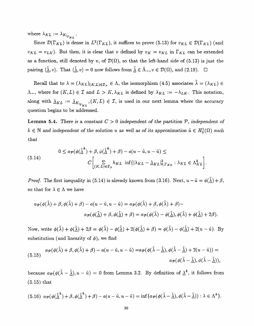
where AK L := AKI .rKL

Since 'D(fKd is dense in L2(fKd, it suffices to prove (5.13) for VKL E 'D(fKd (and

VKL = vLId. But then, it is clear that v defined by VK = VKL in fKL can be extended

as a function, still denoted by v, of 'D(n), so that the left-hand side of (5.13) is just the

pairing (X, v). That (X, v) = 0 now follows from X E fL, V E 'D(n), and (2.19). 0

Recall that to A = (AKd(K,L)EI> E A, the isomorphism (4.5) associates ~ = (AKd E

A_, where for (K,L) E I and L > K,AKL is defined by AKL := -ALK. This notation,

along with lKL := lKI ,(K,L) E I, is used in our next lemma where the accuracyrKL

question begins to be addressed.

Lemma 5.4. There is a constant C > 0 independent of the partition P, independent of

kEN and independent of the solution u as well as of its approximation u E HJ(n) such

that

(5.14)

- k -k0:::; ap(4)(l ) + (3,¢(l ) + (3) - a(u - u,u - u):::;

c[ L; hKL inf{IAKL-lKLI~,rKL :AKLEA1<L]'(K,L)EI>

Proof. The first inequality in (5.14) is already known from (3.16). Next, u - u = 4>(X)+ (3,

so that for A E A we have

ap(4)(~) + (3, 4>(~) + (3) - a(u - U, u - u) = ap(¢(~) + (3, 4>(~) + (3)-

ap( ¢(X) + (3, ¢(X) + (3) = ap( ¢(~) - 4>(X),¢(~) + ¢(X) + 2(3).

Now, write ¢(~) + ¢(X) + 2{3 = ¢(~) - ¢(X) + 2(¢(X) + (3) = ¢(~) - ¢(X) + 2(u - u). By

substitution (and linearity of ¢), we find

(5.15)ap(¢(~) + (3, ¢(~) + (3) - a(u - it, u - u) =ap(4)(~ - X), ¢(~ - X) + 2(u - it» =

ap(¢(~ - X), ¢(~ - X»,because ap(4)(~ - X),u - it) = 0 from Lemma 3.2. By definition of lk, it follows from

(5.15) that

-k -k - - - -(5.16) ap(4)(~ )+{3,¢(l )+{3)-a(u-it,u-11)=inf{ap(¢(A-l),¢(A-~»:AEAk}.

30

Since X E A- by Lemma 5.3, whence ~ - X E A_ for every A E A k, we now infer from

(5.16) and Lemma 5.2 that

(5.17)

-k -ka1'(<p(~ ) + (3, <p(~ ) + (3) - a(u - u,u - u) :::;

C inf{K~/'KIAK - !'Kli,r",r+ (l",r (AK - !,K l) 2/ (L" (lK ) : A E Ak}.For each 1 :::;K ~ N, IAK -lKI~,rK\r splits as the sum LJi)AKL -ll<L15,rKL' Since

the ratios hK / hK L( LEI 1<) are uniformly bounded, (5.17) yields

(5.18)

For (K, L) E I>, let A~(L E A ~<L denote the best L 2 (f K L )-approximation of lK L in

Ak .J( L, l.e.

(5.19)

Since A~<L consists of the polynomials of degree at most kKL ~ 0 in fKL (see (5.2)

and (5.3», the difference A~<L - lK L is always orthogonal to the constant functions in

f1<L, i.e. JrKL ().~<L -ll<L) = O. Both this relation and (5.19) remain valid not only

for (K,L) E I> but also for every pair (K,L) E I since (L,K) E I> if (K,L) 1. I>, and

A~(L = -AttK,lKL = -~LK in this case. Thus, by majorizing the right-hand side of (5.18)

with the special choice AJ(L = ).~(L' the integrals JrJ(\r(A} -lK) vanish and the second

inequality in (5.14) follows at once from (5.19). 0

To complete with, we need an estimate for each infimum appearing in the right-hand

side of (5.14). The following special case of Lemma 4.5 in Babuska and Suri [5] will suffice:

Lemma 5.5. Let s ~ 0 be a real number. There is a constant C > 0 depending only

upon s such that for every integer m ~ 0 and every v E HS(f I( L), we have

(5.20)hmin(m+I,s)

inf{lv - wlo,rKL : w E Pm(fKd}:::; C ~_~ , ,\. Ilvlls.rKL·

31

Actually, in [5] Lemma 5.5 is proved in the two-dimensional case when f J( L is replaced

by a "nondegenerate" triangle or parallelogram. The one-dimensional case considered in

Lemma 5.5 is of course simpler (though not considerably). Also, curiously, the case m = 0

in (5.20) is not considered in [5] although it does not present any particular additional

difficulty.

Since .0 is a polygon, the relation u E Hr(n) should not be expected to hold with r ;::::3

irrespective of the smoothness of f. However, things go differently in any open subset w

ofn such that n \ w is an open neighborhood (in n) of the vertices of n, for then we have

For convenience, we shall refer to r as being the "interior regularity" of u (although it

extends to the boundary away from the vertices). vVeshall also assume that no interface

f J( L contains a vertex of n as an endpoint. This condition often prohibits choosing nJ(as an individual element near the vertices of n, but a small patch will always suffice to

comply with this requirement (Figure 5.1). The net result of this hypothesis is that

(5.21)

provided that A is smooth enough, e.g.

(5.22)

as we shall henceforth assume to fix ideas.

Theorem 5.1. There is a constant C > 0 depending upon the interior regularity r(;::::2) of

u, but independent of the partition P and independent ofu as well as of the approximation

U E HJ(n), such that

(5.23)a( u - u,u - u)I/2 ~ a1'( </>(}/) + (3, </>(~k) + (3)1/2 ~

h2 min(kI<L+I,r-I) II a 112a(u-u,u-u)I/2+C{ ~ J(L . uJ( P/2.(K,L)EI> (kJ(L + 1)2r-3 av~ 3 r

1\ r-2, KL

32

Proof. In Lemma 5.5, let s = r - 3/2,m = kKL and v = aUK/aV~. Then, the conclusion

follows from Lemma 5.4 and elementary manipulations. 0

-k -kTheorem 5.1 reveals the high accuracy of the estimator ap( </>(l ) + ,8, ¢>(l + (3)1/2 for

solutions U having good interior regularity as the finite element mesh is held fixed and k,

i.e. kKL for each pair (K, L) E I>, is increased. Naturally, the difficulties induced by the

lack of smoothness of u in the vicinity of the vertices ofn do not disappear completely since

the norms IIauK / av~ IIr- ~,rK L will usually be larger for interfaces f K L near the corners.

From (5.23), the remedy is to increase kKL along those (and neighboring) interfaces. In

contrast, refining the mesh creates interfaces even closer to the singularity along which

IIauK / av~ IIr- %,r K L increases.

Also, in practice, neither </>(~k) = (</>K(lt-» nor (3 = ((3K) are calculated exactly.

The numerical evaluation of </>K(lt-) and (3K requires solving the local problems (3.9)

and (3.11), respectively, over the sub domains nK, and large angles in nK will affect the

accuracy ,of the local calculations. Note that large angles in some .0K'S will exist if n itself

has such large angles because of the standing assumption that no interfaces f K L terminates

at a vertex of n. However, the accuracy question is easier and cheaper to handle at the

local rather than global level.

-k --kRemark 5.1: Since u - u - </>(l ) - (3 = ¢>(21- 21 ), the method of proof of Theorem 5.1

also yields

(5.24)

- k - k 1/2a( u - it - ¢>(l ) - (3,u - U - ¢>(l ) - (3) :::;

h2rnin(kKL+l,r-I) II a 112c ')' KL UK 1/2{(K,t)'EI> (kKL + 1)2r-3 av~ r-%,rKL} ,

-kl.e. U + ¢>(l ) + (3 is a highly accurate approximation of u as k is increased if u has good

interior regularity r. 0-k

It is clear from (5.24) that u + ¢>(l ) + (3 will provide an enhanced solution (in theory

at least) if the polynomial degrees k KLare large enough. Typically, if it is a piecewise

polynomial of degree at most m, then a(u - u, u - u)I/2 = O(hm) is best possible. It then

33

-kfollows from (5.24) that U + <p(l ) + (3 is theoretically a better approximation than u if

kK L ~ m for each pair (K, L) E I, assuming of course sufficient interior regularity of u.

6. The positive semi definite case.

In this section we investigate the case when (7 = 0 in (3.3). The only, but significant,

difference is that the equivalent problems (3.3) - (3.4) continue to have a unique solution u

while the Fredholm alternative holds for the local problems (3.9) or (3.11) for every index

1 ~ K:::; N such that VK = HI(nK), or, equivalently, µ(fK n r) = O.

The new issue here is that for those indices K, the bilinear form aK(-,') in (3.6) satisfies

aK(vK,wK) = 0 whenever VK or WK is a constant. As a result, the solvabiltiy of (3.9)

requires the extra compatibility condition

(6.1)

and then <PK(>.'[<)is determined modulo a constant. Likewise, (3.11) has solutions if and

only if

(6.2)

and (3[( is determined modulo a constant.

The above suggests modifying the definitions of <p(~), ~ E A_, and (3 = ((3K) so that

<1>( j,) and (3 always exist. A Iit tIe thinking leads to the choices

and

(6.4)

aK((3I(, VK) = inK fVK - In1KI (inK f) (inK VI() - aK(UI(, VK), VVK E HI(nK),

for all those indices K such that VI( = HI(nK). Otherwise, the definition of <PK(AK) and

(3K is unchanged (i.e. given by (3.9) and (3.11), respectively).

34

The existence of 4>K(AI() and /3K in (6.3) and (6.4) is not a problem because the right-

hand sides vanish when VK is constant in nK, but their uniqueness is true only in the space

HI (nK)/ po(nK). vVhen VK =I Hl(nl(), 4>K(Al() and /31{ are unique and Vl( / po(nld =

Vn-. Thus, 4>( ~) and /3 exist and are unique in the space

(6.5)

In this setting, 4> remains linear and continuous if HJ(P)/ Po(P) is equipped with the

quotient norm. In this respect, observe that ap( (v l( ), (w K » is unambiguously defined for

(UK), (WK) E HJ(P)/Po(P) since its value depends only upon the equivalence class of (VK)

and (WK).

It is readily seen that Lemma 3.2 is no longer valid with the new definition of 4>( ~) and

,8, and hence Lemma 3.4 also fails to hold. However, the following variant remains true:

Lemma 6.1. Let ~ E A_, and let ~ and f satisfy the compatibility conditions

(6.6)

for every index 1 ~ J( :::; N such that Vl( = HI (nl( ). Then,

(6.7)

and hence

ap(4)(~) + /3, v) = a(u - u, v), Vv E HJ(n),

ap(4)(~) + /3 - (u - u),v) = 0, Vv E HJ(n).

Proof. From (6.3), (6.4) and (6.6), we have

for every VK E HJ(P). If v E HJ(n) and VK := vlnK

, it follows from (2.19) that ap(4)(~)+

/3, v) = In fv - a( u, v) = a( u - u, v). 0

35

The relevance of the compatibility conditions (6.6) stems from the fact that they hold

when AK := aUK/aV~ and U E HJ(n) is the unique solution of the problem

-\7. (A\7u) = fin n.

\Vith this remark and Lemma 6.1, a routine check reveals that Lemma 3.5 and Theorem 3.1

remain valid if attention is confined to those A E A_ satisfying the compatibility conditions

(6.6) (with the obvious modification that 4>(5..) + (3 E HJ(n)/po(p) in part (i) of Lemma

3.5; this implies 4>(~) + (3 = u - u in HJ(n)/po(p». In particular, X:= (aUK/aV~) E A_appears to be the (unique) minimizer of the functional j in (3.15) in the affine subspace

of A- in which the compatibility conditions (6.6) hold. Thus, X is now characterized by a

constrained minimization problem. This is the only difference with the situation described

in Section 3.

The modifications to the Galerkin approximation procedure described in Section 4 are

obvious: Instead of (4.9), the functional J is now being minimized in the affine subspace

of the space Akin which (using (4.5))

(6.8)

The formula (4.16) (resp. (4.17)) remains unchanged when VJ(o =f. HI(nKo) (resp.

FLo =f. Hl(nLo»' If V](o = HI(n](o)' then (4.16) must be replaced by

(6.9)

aKo(4)Ko('pkoLolr ),0](0) = r pkoLoV](o - -ln1 1(1 PkOLO) (1 VKO)'

Ko JrKOLo ](0 rKoLo OKo

Likewise, if VLo = HI(nLo), then (4.17) becomes

The formulas (4.18) and (4.19) remain unchanged if 4>]«(A]() and 13K are always chosen

to have zero average in n](, and Remark 4.2 (i.e. formula (4.20» may be repeated under

36

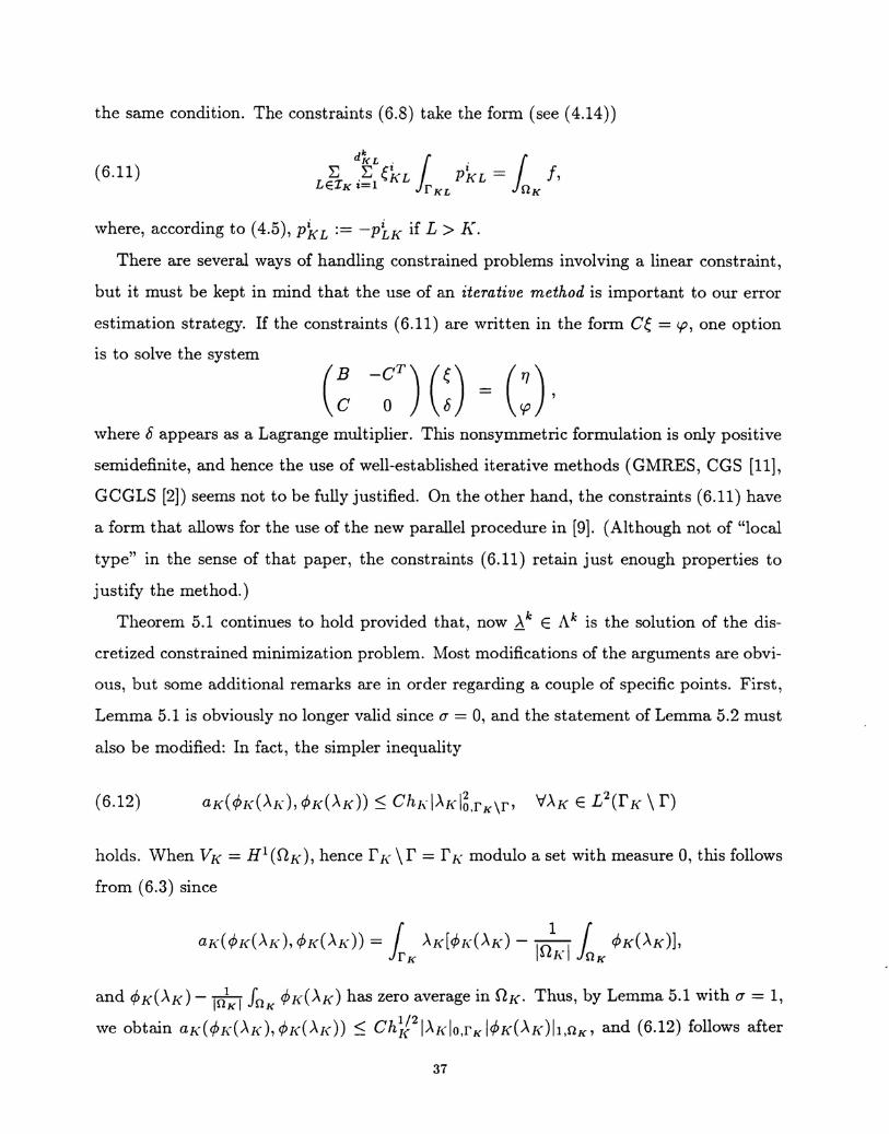
the same condition. The constraints (6.8) take the form (see (4.14»

(6.11)

where, according to (4.5), PkL := -P~K if L > K.There are several ways of handling constrained problems involving a linear constraint,

but it must be kept in mind that the use of an iterative method is important to our error

estimation strategy. If the constraints (6.11) are written in the form C~ = <p, one option

is to solve the system

where 8 appears as a Lagrange multiplier. This nonsymmetric formulation is only positive

semidefinite, and hence the use of well-established iterative methods (GMRES, CGS [11],

GCGLS [2]) seems not to be fully justified. On the other hand, the constraints (6.11) have

a form that allows for the use of the new parallel procedure in [9]. (Although not of "local

type" in the sense of that paper, the constraints (6.11) retain just enough properties to

justify the method.)

Theorem 5.1 continues to hold provided that, now lk E Ak is the solution of the dis-

cretized constrained minimization problem. Most modifications of the arguments are obvi-

ous, but some additional remarks are in order regarding a couple of specific points. First,

Lemma 5.1 is obviously no longer valid since (7 = 0, and the statement of Lemma 5.2 must

also be modified: In fact, the simpler inequality

(6.12)

holds. \Vhen VK = HI(.0 K ), hence f K \ f = f K modulo a set with measure 0, this follows

from (6.3) since

and ¢>K(AK) - If/KI InK ¢>K(AK) has zero average in nK. Thus, by Lemma 5.1 with (7 = 1,

we obtain aK(¢>K(AK),¢>K(AK» ::; Ch~PIAKlo,rKI¢>K(AK)iI,nK' and (6.12) follows after

37

majorizing 14>1({A1()ll,nK by CaK(4)J({AK), 4>K{AJ())I/2 where C > 0 is a constant depend-

ing only upon A and n. When VI( =I HI(nK), the validity of (6.12) was already noticed

in the proof of Lemma 5.2, and the same arguments continue to work when (7 = o.The next point that deserves clarification is the use of Lemma 3.2 for the justification

of (5.15) in the proof of Lemma 5.4. Indeed, as noted earlier, Lemma 3.2 is no longer valid

and hence cannot be used to show that ap(4)(~ - X),u - u) = O. Actually, this relation

need not be true for arbitrary A E A, i.e. arbitrary ~ E A_, but it continues to hold

when the image ~ of A through the isomorphism (4.5) satisfies the constraints (6.6): If

VI( = HI (nJ(), we have

(6.13)

a I( ( 4> J( ( AJ( - lJ( ), UJ( - UJ() = (A J( - ~J(, UK - it K) - In1J(I (A J( - AK, 1) inK (u K - UJ() =

(AK -lK' UK - UJ(),

because (AI(,l) = - InK! = (lK,l) (recall that lI( := aUJ(/av"t satisfies (6.6». If

now VI( =I Hl(nI(), then (6.13) holds by definition of 4>K(AK). Thus, (6.13) holds for

1 :::;J( :::;N if the constraints (6.6) are satisfied, and hence ap(4)(~ - X),u - u) = 0 by

(2.19). Evidently, the choice ,\ = lk is possible since Xksatisfies (6.6), and this is all that

is needed to establish the inequality (simpler than (5.18»

(6.14)

-k -kap(4)(l ) + (3,4>(~ ) +(8) - a(u - U,U - u) :::;

Cinf {~ ~ hI<LI'\KL - ~I\-LI~,rKL : A E Ak, (6.6) hOldS}.I(=ILEIJ(

The key point now is that if A~(L E Aj(L is the best L2(fl(L)- approximation of lKL,

given by (5.19), then A~(L -lKL is orthogonal to the constant functions in fKL, i.e.

};r A~(L -lKL = O. This implies at once that if A~( is defined by ,\~ = A~L' thenKL IrK

IrJ(\r A~( = IrJ(\r lK = InK f· This means that (6.6) holds with A = ,\0 := (A~(). Thus,

the choice A = ,\0 can be used to obtain an upper bound for the right-hand side of (6.14).

Together with (5.19) this now yields the tighter upper bound

38

trivially equivalent to (5.14). In other words, Lemma 5.4 remains valid as stated, and the

arguments of the proof of Theorem 5.1 can be repeated.

-kRemark 6.1: Although 4>(l ) + f3 E HJ (P)/ Po(P) suffices for energy-norm error cal-

culation, a little extra work is needed to obtain an enhanced solution since, obviously,

the constant CK E lR added to any choice of 4>K{A}) + f3K when VK = Hl(nK) (and

CK = 0 otherwise) is important to the quality of (say) the L2(nK)-approximation of UK

by UK + 4>K(Aj() + f3K +CK. Since the solution u is continuous across the interfaces f KL, a

reasonable criterion for the selection of the constants CK is the minimization of the jumps

I4>K(A}) + f3K + CK - 4>L('\i) - f3L - CLI along these interfaces. It can be shown that

minimization relative to the L2(rz)-norm produces a solution 4>(5..k) + f3 + c(c = (CK»

such that lu - U - 4>(5..k) - f3 - clo,n = O(hlu - u - 4>(5..k) - f3ll,n). Details are omitted for

breviety. 0

References ..

[1] Ainsworth, M. and aden, J.T., A unified approach to a posteriori error estimation using element

residual methods, Numer. Math. 65 (1993), 23-50.

[2] Axelsson, 0., A generalized conjugate gradient. least square method, Numer. Math. 51 (1987),209-227.

[3] Babuska, 1., aden, J.T. and Lee, J.K., Mixed-hybrid finite element approximations of second-order

elliptic boundary value problems, Compo Meth. Appl. Mech. Eng. 11 (1977), 175-206.

[4] Babuska, 1., aden, J .T. and Lee, J .K., Mixed-hybrid finite element approximations of second-order

elliptic boundary value problems, Part 2 - Weak hybrid methods. Compo Meth. Appl. Mech. Eng. 14

(1978), 1-22.

[.'>] BabuSka, 1. and Suri, M., The h - p version of the finite element method with quasiuniform meshes,

Math. Mod. Num. Anal. 21 (1987), 199-238.

[6] Bank. R.E;, and Weiser. A., Some a posteriori error estimators for elliptic partial differential equations,

Math. Compo 44 (1985), 283-301.

[7] Ciarlet, P.G., The Finite Element Method for Elliptic Problems, North-Holland, (1978).

[8] Grisvard, P., Elliptic Problems in Nonsmooth Domains, Pitman, (1985).

[9] Layton, \V.J., Maubach, J. M. and Rabier, P.J., Parallel algorithms for maximal monotone operators

of local type, Numer. Math. 71 (1995), 29-58.

[10] Layton, W.J. and Rabier. P.J., Peaceman-Rachford procedure and domain decomposition for finite

element problems, Num. Lin. Alg. Appl. 2 (1995), 363-393.

[11] Sonneveld, P., cas, a fast Lanczos-solver for non-symmetric linear systems, SIAM J. Sci. Stat. Compo

10 (1989), 36-52.

39