N94-23645A DIRECT APPROACH TO FINDING UNKNOWN

BOUNDARY CONDITIONS IN STEADY HEAT CONDUCTION

Thomas J. Martin* and George S. Dulikravich**

Department of Aerospace EngineenngThe Pennsylvania State University, University Park, PA 16802, USA

SUMMARY

The capability of the boundary element method (BEM) in determining thermal boundaryconditions on surfaces of a conducting solid where such quantities are unknown has been

demonstrated. The method uses a non-iterative direct approach in solving what is usually called theinverse heat conduction problem (IHCP). Given any over-specified thermal boundary, conditionssuch as a combination of temperature and heat flux on a surface where such data is readily available,the algorithm computes the temperature field within the object and an,,, unknown thermal'boundary

conditions on surfaces where thermal boundary values are unavailable'. A two-dimensional, steady-state BEM program has been developed and was tested on several simple geometries ',,,'here the

analytic solution was known. Results obtained with the BEM were in excellent agreement with theanal_'tic values. The algorithm is highly flexible in treating complex geometries, mixed thermal

boundar2,' conditions and temperature-dependent material properties and is presently being extcndcdto three-dimensional and unsteady heat conduction problems. The accuracy and rei'iabilitv of thistechnique was very good but tended to deteriorate when the known surface'conditions were onlyslightly over-specified and far from the inaccessible surface.

INTRODUCTION

The objective of the steady-state inverse heat conduction problem is to deduce temperaturesand heat fluxes on any surface or surface element where such information is unknown. In manyinstances it is impossible to place sensors and take measurements on a particular surface of aconducting solid due to the inaccessibility or severity of the environment on that surface. Theseunknown thermal boundary values may be deduced "from additional temperature or heat flux

measurements made within the solid or on some other surface of the solid. This problem has beengiven a considerable amount of attention bv a variety of researchers and virtually all work has beendirected to the one-dimensional transient problem. :l'he first method proposed t'o solve the IHCF :)

used inversion of convolution integrals (Stolz 1960) and was subsequently improved by a numberof authors (Beck et al. 1988). Many other methods have also been developed using suchtechniques as Laplace transforms, finite elements, time-marching finite differences and other

approaches. A detailed chronological review of the IHCP literature has been provided by Hensel(1992). -

A characteristic of most of these inverse techniques is that they tend to produce temporaloscillations in the unknown surface thermal condition estimates that are larger than the temporaloscillations in the over-specified thermal data as it propagates through the solid (Hills and Hensel

1986). In other words, the random noise due to round off errors tends to magnify as the solutionproceeds and quickly produces a useless solution, especially as the distance between the surface

and the over-specified information increases. A number of authors have presented varioussmoothing techniques for reducing this error growth, but the effect of these operations on theaccuracy of the solution is not easy to evaluate (Murio 1993).

Graduate research assistant.

Associate professor.

137

https://ntrs.nasa.gov/search.jsp?R=19940019172 2018-09-01T03:47:11+00:00Z

Themethodpresentedhereindoe_notutilizeanyartificialsmoothingtechniqueandisnotlimited to transientor one-dimensionalproblems.Thisapproachis non-iterativeandhasbeenshownto computemeaningfulandaccuratethermalfieldsin asingleanalysisusingastraight-forwardmodificationto theboundaryelementmethod(BEM).

TheBEM is averyaccurateandefficienttechniquethatcansolveboundarT.valueproblemssuchasthosegoverningheatconduction,electromagneticfields,irrotationalincompressiblefluidflow, elasticity,andmanyotherphysicalphenomenon.Forsteady-stateheatconductionanalysisusingtheBEM, either temperatures, T, or heat fluxes, Q, are specified everywhere on the surface ofthe solid where one of these quantities is known while the other is unknown. In the BEM solution

to the IHCP, both T and Q must be specified on a part of the solid's surface, while both T and Q areunknown on another part of the surface. Elsewhere on the solid's surface, normal boundary

conditions should be applied as either T's or Q's. The surface section where both T and Q arespecified simultaneously is called the over-specified boundary and is necessary for the IHCPproblem's solution.

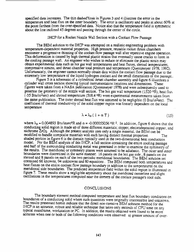
Figure 1 illustrates a typical two-dimensional, multiply Connected, inverse heat conduction

problem. Surfaces labeled I"1 are the over-specified boundaries where both T and Q are given.

Normal boundary conditions (either T or Q specified) are enforced on the surfaces labeled I" 2.

Thermal data is assumed to be inaccessible on the inner 1"3 surface and thus has both T and Qunknown on this boundary. The objective of the IHCP is to compute temperatures and heat fluxes

on the boundary F3 using only the values ofT and Q provided on the surface of the solid and,possibly, additional temperature measurements made within the solid if such data is available.

THEORY

Two-Dimensional Steady-State BEM

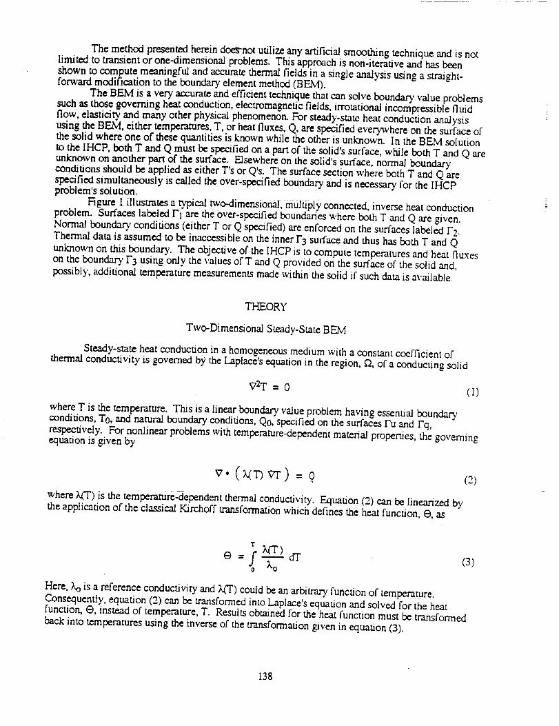
Steady-state heat conduction in a homogeneous medium with a constant coefficient ofthermal conductivity is governed by the Laplace's equation in the region, Q, of a conducting solid

V2T = 0 (1)

where T is the temperature. This is a linear boundary value problem having essential boundaryconditions, TO, and natural boundary conditions, Q0, specified on the surfaces Fu and Fq,

respectively. For nonlinear problems with temperature-dependent material properties, the governingequation is given by

v. w) = o (2)

where X(T) is the temperature-dependent thermal conductivity. Equation (2) can be Iineariz._ bythe application of the classical Kirchoff transformation which defines the heat function, e, as

T xfr)e =f- 7-o

0(3)

Here, Xo is a reference conductivity and Z_I") could be an arbitrary function of temperature.Consequently, equation (2) can be transformed into Laplace's equation and solved for the heatfunction, e, instead of temperature, T. Results obtained for the heat function must be transformed

back into temperatures using the inverse of the transformation given in equation (3).

138

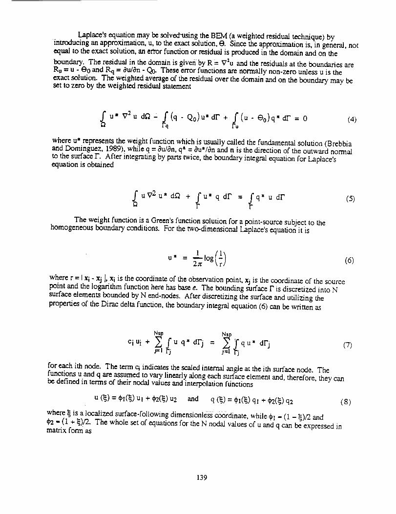
Laplace'sequationmaybesolved-usingtheBEM (aweightedresidualtechnique)byintroducinganapproximation,u, to theexactsolution,O. Sincetheapproximationis, in general,notequalto theexactsolution,anerrorfunctionor residualisproducedin thedomainandon theboundary.Theresidualin thedomainisgivenbyR = V2u andtheresidualsat theboundariesareRu= u - O0 and Rq = au/an - Qo. These error functions are normally non-zero unless u is the

exact solution. The weighted average of the residual over the domain and on the boundary may beset to zero by the weighted residual statement

fu*V:udf_ fq(q-Qo)u*dr'+ r,,f(u'e°)q*dr= 0 (4)

where u* represents the weight function which is usually called the fundamental solution (Brebbiaand Dominguez, 1989), while q = au/an, q* = au*/On and n is the direction of the outward normal

to the surface F. After integrating by parts twice, the boundary integral equation for Laplace'sequation is obtained

fuV2u*d_ + rfu*qdF = rfq*udl" (5)

The weight function is a Green's function solution for a point-source subject to thehomogeneous boundary conditions. For the two-dimensional Laplace's equation it is

u * = _--_log (6)

where r = I xi - xj l, xi is the coordinate of the observation point, xj is the coordinate of the sourcepoint and the logarithm function here has base e. The bounding surface F is discretized into N

surface elements bounded by N end-nodes. After discretizing the surface and utilizing the

properties of the Dime delta function, the boundary integral equation (6) can be written as

ciui+ _°Suq'dF j = _'fqu* dFj (7)

3=1 _r'j j=l l"j

for each ith node. The term ci indicates the scaled internal angle at the ith surface node. The

functions u and q are assumed to vary linearly along each surface element and, therefore, they canbe defined in terms of their nodal values and interpolation ftinctions

u (_) = ¢u(_) ul + ¢z(_) u2 and q (_) = ¢_1(_) ql + 02(_) q2 (8)

where _ is a localized surface-following dimensionless coordinate, while 91 - (1 - _)/2 and

q2 - (1 + _)/2. The whole set of equations for the N nodal values of u and q can be expressed inmatrix form as

139

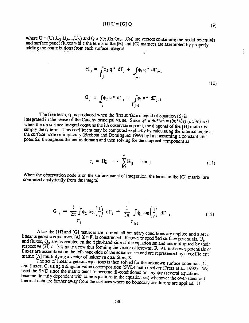
u = [G] Q (9)

where U = (UI,U2,U3 .... ,UN) and Q = (Q1,Q2,Q3 ..... QN) are vectors containing the nodal potentialsand surface panel fluxes while the terms in the [H] and [G] matrices are assembled by properlyadding the contributions from each surface integral .....

H,j= f,: q* drj ÷ q• dFj+ Irj Fj+t

(I0)

a 0 = f,.. u* drj + f'h u* drj._Fj Fj +I

The free term, q, is produced when the first surface integral of equation (6) isintegrated in the sense of the Cauchy principal value. Since q* = du*/0n = (au*/ar) (0r/0n) = 0

when the ith surface integral contains the ith observation point, the diagonal of the [H] mat-ix is

simply the ci term. This coefficient may be computed explicitly by calculating the internal angle atthe surface node or implicitly (Brebbia and Dominguez 1989) by first assuming a constant unitpotential throughout the entire domain and then solving for the diagonal component as

N

ci = Hii = _._Hij i,, j (11)

When the observation node is on the surface panel of integration, the terms in the [G] matrix arecomputed analytically from the integral

_ 1 fq_21og(1 _ 1 (1_G ii--_" r/ dr_ + o--A"f_l°g r: dr_+_

F i r'i+ 1

(12)

After the ['t.l'J and [G] matrices are formed, all boundary conditions are applied and a set of

linear algebraic equations, [A] X = F, is constructed. Known or specified surface potentials, Uj,and fluxes, Qj, are assembled on the right-hand-side of the equation set and are multiplied by theirrespective [HI or [G] matrix row thus forming the vector of knowns, F. All unknown potentials orfluxes are assembled on the left-hand-side of the equation set and are represented by a coefficientmatrix [A] multiplying a vector of unknown quantities, X.

The set of linear algebraic equations is then solved for the unknown surface potentials, U,and fluxes, Q, using a singular value decomposition (SVD) matrix solver (Press et al. 1992). Weused the SVD since the matrix tends to become ill-conditioned or singular (several equationsbecome linearly dependent with other equations in the equation set) whenever the over-specifiedthermal data are farther away from the surfaces where no boundary conditions are applied. If

140

additionalthermaldatawithin thesolid is=provided, additional equations may be added to theequation set. Note that the SVD algorithm is capable of providing a satisfactory solution vectoreven when the [,4,] matrix is not square. The more rows (i.e. more data points) that are provided tothe system, the more accurate the solution vector becomes, although the reverse is true when thematrix has less rows than columns. Once the matrix is solved, the entire thermal field within thesolid can be easily deduced.

RESULTS AND DISCUSSION

IHCP for a Square Plate Using the BEM

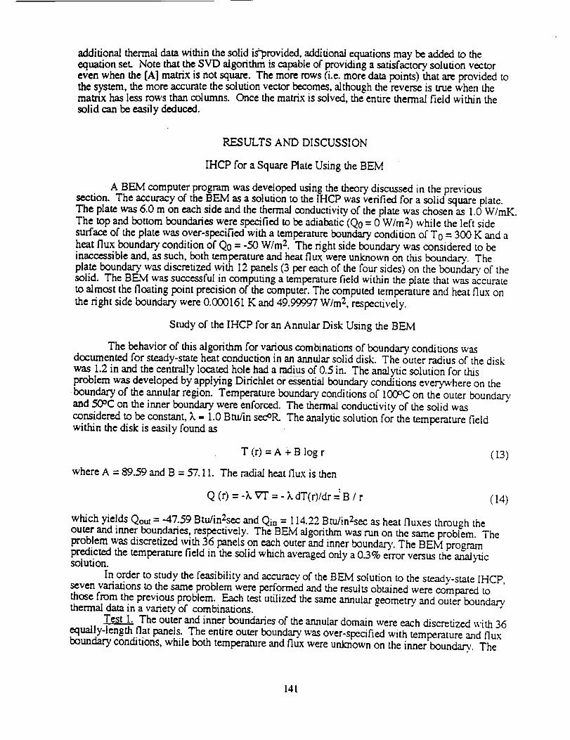
A BEM computer program was developed using the theory discussed in the previoussection. The accuracy of the BEM as a solution to the IHCP was verified for a solid square plate.The plate was 6.0 m on each side and the thermal conductivity of the plate was chosen as 1.0 W/mK.

The top and bottom boundaries were specified to be adiabatic (Q0 = 0 W/m 2) while the left side

surface of the plate was over-specified with a temperature boundary condition ofT0 = 300 K and a

heat flux boundary condition of Q0 = -50 W/m 2. The fight side boundary was considered to beinaccessible and, as such, both temperature and heat flux were unknown on this boundary. Theplate boundary was discretized with 12 panels (3 per each of the four sides) on the boundar}' of thesolid. The BEM was successful in computing a temperature field within the plate that was accurateto almost the floating point precision of the computer. The computed temperature and heat flux on

the fight side boundary were 0.030161 K and 49.99997 W/m 2, respectively.

Study of the IHCP for an Annular Disk Using the BEM

The behavior of this algorithm for various combinations of boundary conditions wasdocumented for steady=state heat conduction in an annular solid disk. The outer radius of the disk

was 1.2 in and the centrally located hole had a radius of 0.5 in. The analytic solution for thisproblem was developed by applying Dirichlet or essential boundary conditions everywhere on the

boundary of the annular region. Temperature boundary conditions of 100oc on the outer boundaryand 50°C on the inner boundary were enforced. The thermal conductivity of the solid was

considered to be constant, k = 1.0 Btu/in see'OR. The analytic solution for the temperature fieldwithin the disk is easily found as

T (r) =A + B log r

where A = 89.59 and B = 57.11. The radial heat flux is then

(13)

Q (r) : -_. vT" = - k dT(r)/dr : B / r (14)

which yields Qout = -47.59 Btu/in2sec and Qia : 1 I4.22 Btu/in2sec as heat fluxes through theouter and inner boundaries, respectively. The BEM algorithm was run on the same problem. Theproblem was discretized with 36 panels on each outer and inner boundary. The BEM programpredicted the temperature field in the solid which averaged only a 0.3% error versus the anal2,aicsolution.

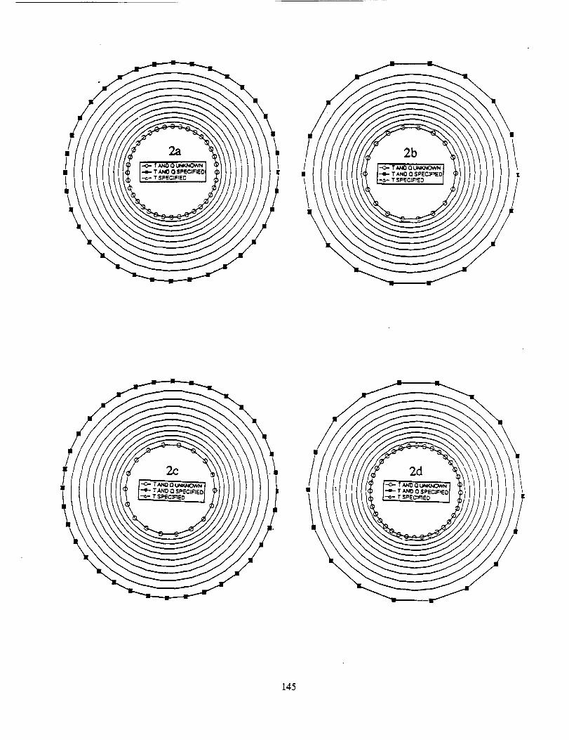
In order to study the feasibility and accuracy of the BEM solution to the steady-state IHCP,seven variations to the same problem were perform_ and the results obtained were compared tothose from the previous problem. Each test utilized the same annular geometry, and outer boundarythermal data in a variety of combinations.

Test I. The outer and inner boundaries of the annular domain were each discretized with 36

equally-length flat panels. The entire outer boundary was over-specified with temperature and fluxboundary conditions, while both temperature and flux were unknown on the inner boundary. The

141

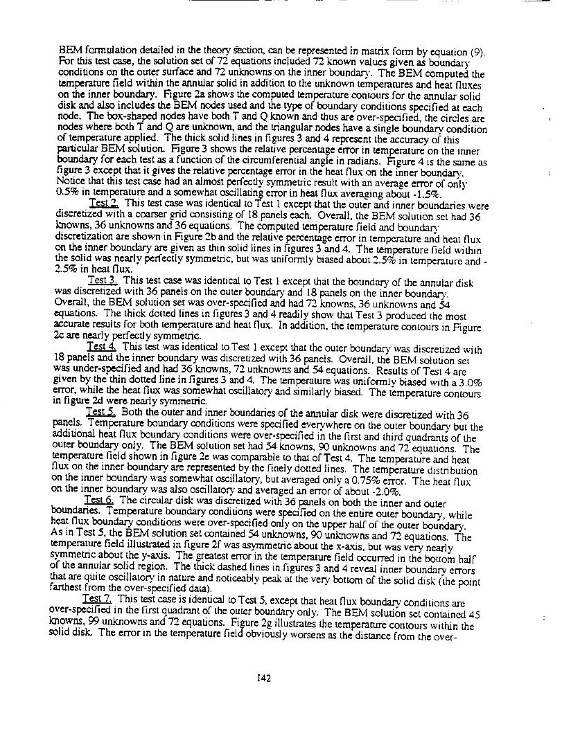
BEM formulationdetailedin thetheorygection, can be represented in matrix form by equation (9).For this test case, the solution set of 72 equations included 72 known values given as boundar3"conditions on the outer surface and 72 unknowns on the inner boundary. The BEM computed thetemperature field within the annular solid in addition to the unknown temperatures and heat fluxeson the inner boundar3'. Figure 2a shows the computed temperature contours for the annular solid

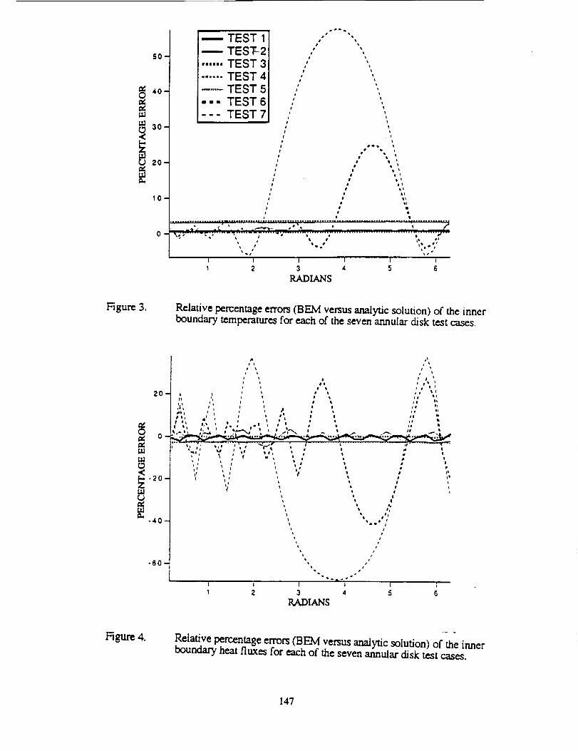
disk and also includes the BEM nodes used and the type of boundary, conditions specified at eachnode. The box-shaped nodes have both T and Q known and thus are over-specified, the circles arenodes where both T and Q are unknown, and the triangular nodes have a single boundary, conditionof temperature applied. The thick solid lines in figures 3 and 4 represent the accuracy of thisparticular BEM solution. Figure 3 shows the relative percentage error in temperature on the innerboundary for each test as a function of the circumferential angle in radians. Figure 4 is the same asfigure 3 except that it gives the relative percentage error in the heat flux on the inner boundarn,.

Notice that this test case had an almost perfectly symmetric result with an average error of only0.5% in temperature and a somewhat oscillating error in heat flux averaging about -1.5%.

This test case was identical to Test 1 except that the outer and inner boundaries werediscretized with a coarser grid consisting of 18 panels each. Overall, the BEM solution set had 36

knowns, 36 unknowns and 36 equations. The computed temperature field and boundaQdiscretization are shown in Figure 2b and the relative percentage error in temperature and heat fluxon the inner boundary are given as thin solid lines in figures 3 and 4. The temperature field withinthe solid was nearly perfectly symmetric, but was uniformly biased about 2.5% in temperature and -2.5% in heat flux.

Test3________.This test case was identical to Test 1 except that the boundary of the annular disk

was discretized with 36 panels on the outer boundary and 18 panels on the inner boundary.Overall, the BEM solution set was over-specified and had 72 knowns, 36 unknowns and 54

equations. The thick dotted lines in figures 3 and 4 readily show that Test 3 produced the most

accurate results for both temperature and heat flux. In addition, the temperature contours in Figure2.c are nearly perfectly symmetric.

This test was identical to Test 1 except that the outer boundary was discretized with18 panels and the inner boundary was discretized with 36 panels. Overall, the BEM solution setwas under-specified and had 36 knowns, 72 unknowns and 54 equations. Results of Test 4 aregiven by the thin dotted line in figures 3 and 4. The temperature was uniformly biased with a 3.0%error, while the heat flux was somewhat oscillatory and similarly biased. The temperature contoursin figure 2d were nearly symmetric.

Both the outer and inner boundaries of the annular disk were discretized with 36panels. Temperature boundary conditions were specified everywhere on the outer boundary but the

additional heat flux boundary conditions were over-specified in the first and third quadran_ of theouter boundary only. The BEM solution set had 54 knowns, 90 unknowns and 72 equations. Thetemperature field shown in figure 2e was comparable to that of Test 4. The temperature and heatflux on the inner boundary, are represented by the finely dotted lines. The temperature distributionon the inner boundary was somewhat oscillatory, but averaged only a 0.75% error. The heat fluxon the inner boundary was also osciliator2,' and averaged an error of about -2.0%.

Test 6......._._,The circular disk was discretized with 36 panels on both the inner and outer

boundaries. Temperature boundary conditions were specified on the entire outer boundary, while

heat flux boundary conditions were over-specified only on the upper half of the outer boundary.As in Test 5, the BEM solution set contained 54 unknowns, 90 unknowns and 72 equations. The

temperature field illustrated in figure 2f was asymmetric about the x-axis, but was very nearlysymmetric about the y-axis. The greatest error in the temperature field occurred in the bottom halfof the annular solid region. The thick dashed lines in figures 3 and 4 reveal inner boundary errors

that are quite oscillatory in nature and noticeably peak at the very bottom of the solid disk (the pointfarthest from the over-specified data).

Test 7. This test case is identical to Test 5, except that heat flux boundary conditions areover-specified in the first quadrant of the outer boundary only. The BEM solution set contained 45

knowns, 99 unknowns and72 equations. Figure 2g illustrates the temperature contours within thesolid disk. The error in the temperature field obviously worsens as the distance from the over-

142

specifieddataincreases.Thethindashefflinesin Figures3 and 4 illustrate the error in thetemperature and heat flux on the inner boundary. The error is oscillatory and peaks at about 60% atthe point farthest from the over-specified data. Notice also that the temperature field is symmetricabout the line inclined 45 degrees and passing through the center of the circle.

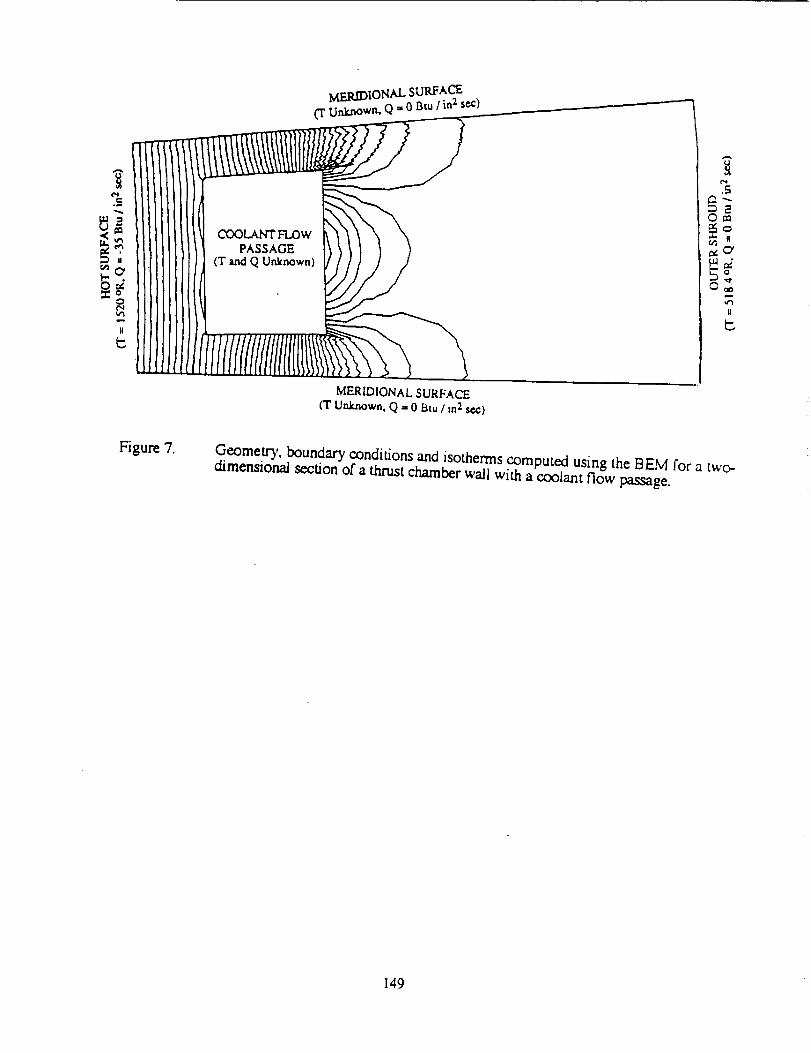
IHCP for a Rocket Nozzle Wall Section with a Coolant Flow Passage

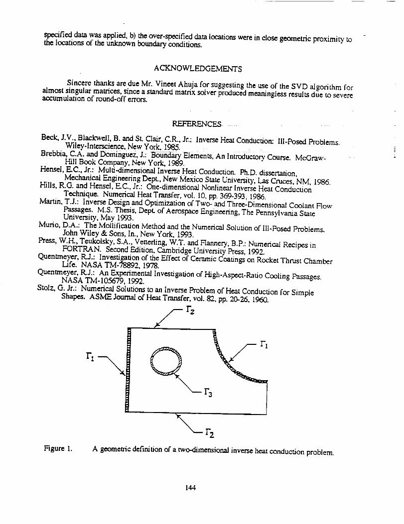
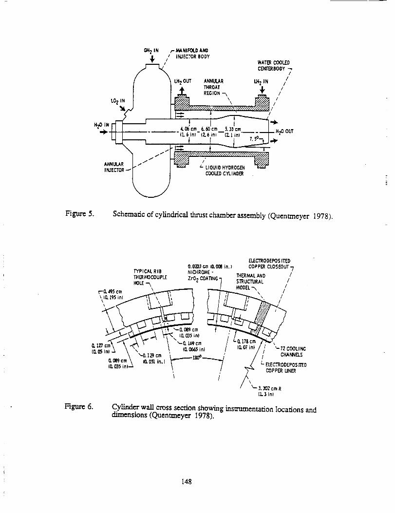
The BEM solution to the IHCP was attempted on a realistic engineering problem withtemperature.dependent material properties. High pressure, reusable rocket thrust chambersencounter a progressive thinning of the coolant flow passage wall after repetitive engine operation.This deformation is caused by high thermal plastic strains that eventually cause cracks to form inthe cooling passage wall. An engineer who wishes to reduce or eliminate the plastic strain mayobtain experimental data such as hot gas wall temperatures and heat fluxes, shroud temperatures,compressive strains, and thrust chamber total pressure and temperature (Quentmeyer 1978, 1992).Unfortunately, the engineer cannot normally obtain data within the coolant flow passage due to the

extremely low temperature of the liquid hydrogen coolant and the small dimensions of the passage.._gure 5 is a schematic of a cylindrical thrust chamber assembly and figure 6 illustrates a

cylinder wall cross section showing typical instrumentation locations and dimensions. These

figures were taken from a NASA publication (Quentmeyer 1978) and were subsequently used to

generate the geometry, of the nozzle wall section. The hot gas wall temperature (1520 °R), heat flux

(-35 Btu/inZsec) and shroud temperature (518.4 °R) were experimental measurements taken from

the same publication. The outer shroud heat flux was assumed to be negligible (0 Btu/in2sec). Thecoefficient of thermal conductivity of the solid copper region was linearly dependent on the localtemperature

_.-_o( I + (xT) (15)

where ko - 0.004893 Btu/insec°R and a = -0.000055056 oR-l. In addition, figure 6 shows that the

conducting solid region is made up of three different materials; copper, electrodeposited copper, andnichrome ZrO2. Although the present analysis uses only a single material, the BEM can be

modified to handle composite materials with each having distinct thermal properties. Theshaded portion in figure 6 is the domain typically used in the two-dimensional heat conduction

model. For the BEM analysis of this IHCP, a full section containing the entire cooling passageand half of the surrounding conducting metal was generated in order to examine the symmetry, ofthe results. The meridional or symme.try planes were assumed to be adiabatic. The outer and innerboundaries were discretized in the same manner:. 16 panels on the hot gas side, 8 panels on theshroud and 8 panels on each of the two periodic meridional boundaries. The BEM solution set

contained 66 knowns, 94 unknowns and 80 equations. The BEM computed both temperatures andheat fluxes on the entire coolant flow passage boundary in addition to the temperatures on themeridional side boundaries. The predicted temperature field ,;vithin the solid region is illustrated infigure 7. These results show a negligible asymmetry, about the meridional centertine and slightoscillations in the temperatures computed near the comers of the coolant passage's cool side.

CONCLUSIONS

The boundary, element method computed temperature and heat flux boundary conditions onboundaries of a conducting solid where such quantities were originally inaccessible and unknown.The results presented herein indicate that the direct non-iterative BEM solution method for the

IHCP is an accurate, robust and reliable technique that takes only seconds of CPU time on an3'typical mainframe, workstation or PC. In addition, the results otJtained were found to be more

accurate when one or both of the following conditions were obsem, ed: a) greater amount of over-

143

specified data was applied, b) the over-specified data locations were in close geometric proximity tothe locations of the unknown boundary conditions.

ACKNOWLEDGEMENTS

Sincere thanks are due Mr. Vineet Ahuja for suggesting the use of the SVD algorithm foralmost singular matrices, since a standard matrix solver produced meaningless results due to severeaccumulation of round-off errors.

REFERENCES

Beck, J.V., Blaclovell, B. and St. Clair, C.R., .Jr.: Inverse Heat Conduction: Ill-Posed Problems.Wiley-lnterscience, New York, 19fl5.

Brebbia, C.A. and Dominguez, J.: DoundaryElements, An Int_uctorv Course. McGraw-Hill Book Company, New York, 1989.

Hensel, EC., 2r.: Multi-dimensional Inverse Heat Conduction. Ph.D. dissertation,

Mechanical Engineering Dept., New Mexico State University, Las Cruces, NM, 1986.Hills, R.G. and Hensel, EC., Jr.: One-dimensional Nonlinear Inverse Heat Conduction

Techmque. Numerical Heat Transfer, vo[. I0, pp. 369-393, 1986.Martin, T.2.: Inverse Design and Optimization oFTwo- and Three-Dimensional Coolant Row

Passages. M.S. Thesis, Dept. of Aerospace Engineering, The Pennsylvania StateUniversity, May 1993.

Murio, D.A.: The Mollification Method and the Numerical Solution of Ill-Posed Problems.John Wiley & Sons, In., New York, 1993.

Press, W.H., Teukolsky, S.A., Vetteding, W.T. and FIannery, B.P.: Numerical Recipes inFORTRAN. Second Edition, Cambridge University Press, 1992.

Quentmeyer, R.J.: Investigation of the Effect of Ceramic Coatings on Rocket Thrust ChamberLife. NASA TM-78892, 1978.

Quentmeyer, R..2.: An Experimental Investigation of High-Aspect-Ratio Cooling Passages.NASA TM-I05679, 1992.

Stolz, G. 2r.: Numerical Solutions to an Inverse Problem of Heat Conduction for SimpleShapes. ASM]E .Journal of Heat Transfer, vol. 82, pp. 2@26, 1960.

Figure I. A geometric definition of a two-dimensional inverse heat conduction problem.

144

/

I

t

145

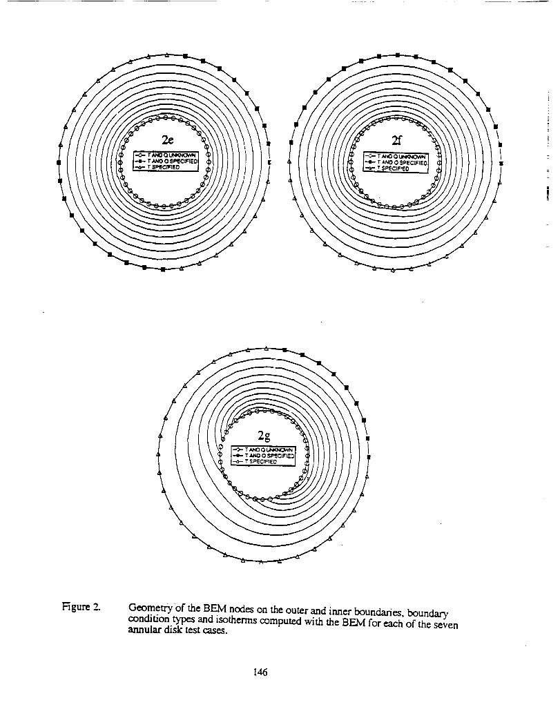
Figure 2.Geometry of the BEM nodes on the outer and inner boundaries, boundarycondition types and isotherms computed with the BEM for each of the sevenannular disk test cases.

146

IZUJuJ

50-

40-

30-

2O

10

---,TEST1

_TES_2,. .... TEST3

...... TEST4

........ TEST5--- TEST6

--- TEST 7 #r

]

/r

/#

i

s

## "_,4

ee _

1

i

o* • I• I

B# • I

! w • i

ii

iI • 1

tl

ttl .................. _,.... ,,,.,-_ -,,.,, - - -,r _ • - -- -- ...... _, ........ --, .......................... -,, ...... ,- ...............

I I ! I I I

2 3 4 5 6

RAD[AHS

Figure 3. Relative percentage errors (BEM versus analytic solution) of the innerboundary temperatures for each of the seven annular disk test cases.

20 _ 1 ' ' • • '' _'

I _,, , , , ' _, , , ,, "|; ,11 I, 11 ' ' - ' ' '1 .....

' I I, _ _ _ • I t P 1 I I I# •

,,, ,, , ,,....

._ ,, ',, , ,, . , ,,t i•_u - , ',, ." / ,

,; ,, ,4 !

I'_1o _ 0 _ ,

-60 " '

I I I I I i

2 3 4 5 6

RAD[ANS

Figure 4.Relative percentage errors (BEM versus analytic solution) of the innerboundary heat fluxes for each of the seven annular disk test cases.

147

GH_ IN ,,- MANIFOLDAND

/ INJECTORBODY_l WAI_ COOL[D

C[NI'ERBODY"7

U.I, OUT ANNULAR LH IN /{ 1 AL THROAT _ //

I I / REGION-,, T /

..J I W//////;//////z_ ;./////////.__/////A /

4.06cm 6.60crn S.33cm HII I -_-,%°,-,,.,,.:-?dY._'-?=--[- _o_

"1 _'""""_//_• _._,;,_% _1"- I _ l- LIOUID HYDROGEN v.gg_

INJECTOR--" __ C00LF.OCYLINDER

Figure 5. Schematic of cylindrical thrust chamber assembly (Quentmeyer 1978).

ELECTRODEPOSflED

0.0203 cm (0.008 in.) COPPERCLOSEOUT7TYPICAL RIB NICHROME- 11-IF..RMALAND /

TH_MOCOUP_ ZrOz COA_NG7 STRUCTURAL /HOLE--_ MODEL_ /

\\(0. 195in_ \ /_ 1 / ]/I _ I/

m _-0, lb9 cm0. 127¢ . (_ 07 inl / _ 7Z((_ I,_ In/ _ _. , _ ,

_9 cm (n 05'1in. ] ---'1

/ _'- _. _0_ cmR(L3 im

Figure 6. Cylinder wall cross sccdon showing instrumentation locations anddimensions (Quentmeyer 1978).

148

O

I!

MERIDIONAL SURFACE

T Unknown, Q = 0 Btu Iin_ scc)

COOLANT FLOW

PASSAGE

(T and Q Unknown)

MERIDIONAL SURFACE

(T Unknown, Q = 0 Btu I in2sec)

II

@,

oOm

II

Figure 7.Geometry, boundary conditions and isotherms computed using the BEM for a two-dimensional section of a thrust chamber wail with a coolant flow passage.

149