2976 OPTICS LETTERS / Vol. 34, No. 19 / October 1, 2009

Bound states of one-, two-, and three-dimensionalsolitons in complex Ginzburg–Landau

equations with a linear potential

Y. J. He,1,2 Boris A. Malomed,3 Dumitru Mihalache,4 B. Liu,1 H. C. Huang,1 H. Yang,1 and H. Z. Wang1,*1State Key Laboratory of Optoelectronic Materials and Technologies, Sun Yat-Sen University, 510275,

Guangzhou, China2School of Electronics and Information, Guangdong Polytechnic Normal University, 510665 Guangzhou, China

3Department of Physical Electronics, School of Electrical Engineering, Faculty of Engineering,Tel Aviv University, Tel Aviv 69978, Israel

4Horia Hulubei National Institute for Physics and Nuclear Engineering (IFIN-HH), 407 Atomistilor,Magurele-Bucharest, 077125, Romania

*Corresponding author: stswhz@mail.sysu.edu.cn

Received June 3, 2009; revised September 12, 2009; accepted August 27, 2009;posted September 9, 2009 (Doc. ID 112096); published September 25, 2009

We analyze interactions between moving dissipative solitons in one- and multidimensional cubic-quinticcomplex Ginzburg–Landau equations with a linear potential and effective viscosity. The interactions be-tween the solitons are analyzed by using balance equations for the energy and momentum. We demonstratethat the separation between two solitons forming a bound state decreases with the increase of the slope ofthe linear potential. © 2009 Optical Society of America

OCIS codes: 190.0190, 190.5530.

Various methods have been clarified for the control ofinteractions between spatial solitons in Kerr media[1,2] and between dissipative solitons [3–8]. These in-teractions are frequently destructive in models basedon the cubic-quintic (CQ) complex Ginzburg–Landau(CGL) equations [9,10].

In this Letter, we study interactions between mov-ing solitons in the 1D, 2D, and 3D equations of theCQ CGL type, which include a combination of a lin-ear potential (alias linear refractive index modula-tion, LRIM, in terms of optics) and effective diffusion(viscosity). Analytical considerations and direct simu-lations reveal stable bound states of such solitons,aligned along the potential’s slope. The separationbetween bound solitons decreases with the increaseof the slope.

We consider the CQ CGL equation for the propaga-tion of an electromagnetic field with local amplitudeu in an optical medium [11]:

iuz + �1/2��u + �u�2u − ��u�4u = iR�u� − �xu, �1�

where �=�2 /�x2+�2 /�y2+�2 /�t2 is the transverseLaplacian. Further, � accounts for the quintic self-defocusing, and R�u�=−�u+��u+��u�2u−��u�4u,where � and µ represent the linear and quintic losses,� is the cubic-gain coefficient, and � is the effectiveviscosity [12–14]. The last term in Eq. (1) accountsfor the LRIM [4,15].

We use the following isotropic ansatz for solitons inthe general 3D case [11]:

u = A�z�exp�−�x − q�z��2 + y2 + t2

2w2�z�+ i��z�

+ ic�z���x − q�z��2 + y2 + t2� + iL�z��x − q�z��� , �2�

0146-9592/09/192976-3/$15.00 ©

and its straightforward reductions in the 2D and 1Dcases. Here, A, w, c, and � represent the amplitude,width, wavefront curvature, and overall phase, re-spectively. Peak position q�z� and conjugate momen-tum L�z� account for the motion of the soliton alongthe x direction.

We resort to the method elaborated in [9] to ana-lyze possibilities for the control of soliton interac-tions, using the evolution equations for the energy,E=�−

�− �−

�u�x ,y , t��2dxdydt, and x component ofthe momentum, M= �i /2��−

+�−+�−

+�uxu*−ux*u�dxdydt,

which can be easily derived in the general form [16]

dE

dz=

−

+ −

+ −

+

�u*G + uG*�dxdydt, �3�

dM

dz= i

−

+ −

+ −

+

�ux*G − uxG*�dxdydt, �4�

where G=R�u�+ i�xu. We take a configuration in theform of a pair of far-separated solitons:

u�x,y,t� = u0�x − x0/2,y,t�exp�i� + u0�x + x0/2,y,t�,

�5�

where u0�x ,y , t� is a stable solution of Eq. (1), x0 is theseparation between the two solitons in the x direc-tion, and is the initial phase difference betweenthem. For stationary solutions, the corresponding so-lutions must satisfy energy- and momentum-balanceequations,

dE�u0,x0,��/dz = dM�u0,x0,��/dz = 0. �6�

From here, we find the equilibrium value of the con-jugate momentum: L=�w2 / �2��1+4c2w4��. At the ini-tial stage, the soliton moves with an acceleration in

the x direction, under the action of the driving force

2009 Optical Society of America

October 1, 2009 / Vol. 34, No. 19 / OPTICS LETTERS 2977

induced by the LRIM. However, the viscous frictionforce leads to the establishment of the dynamic equi-librium.

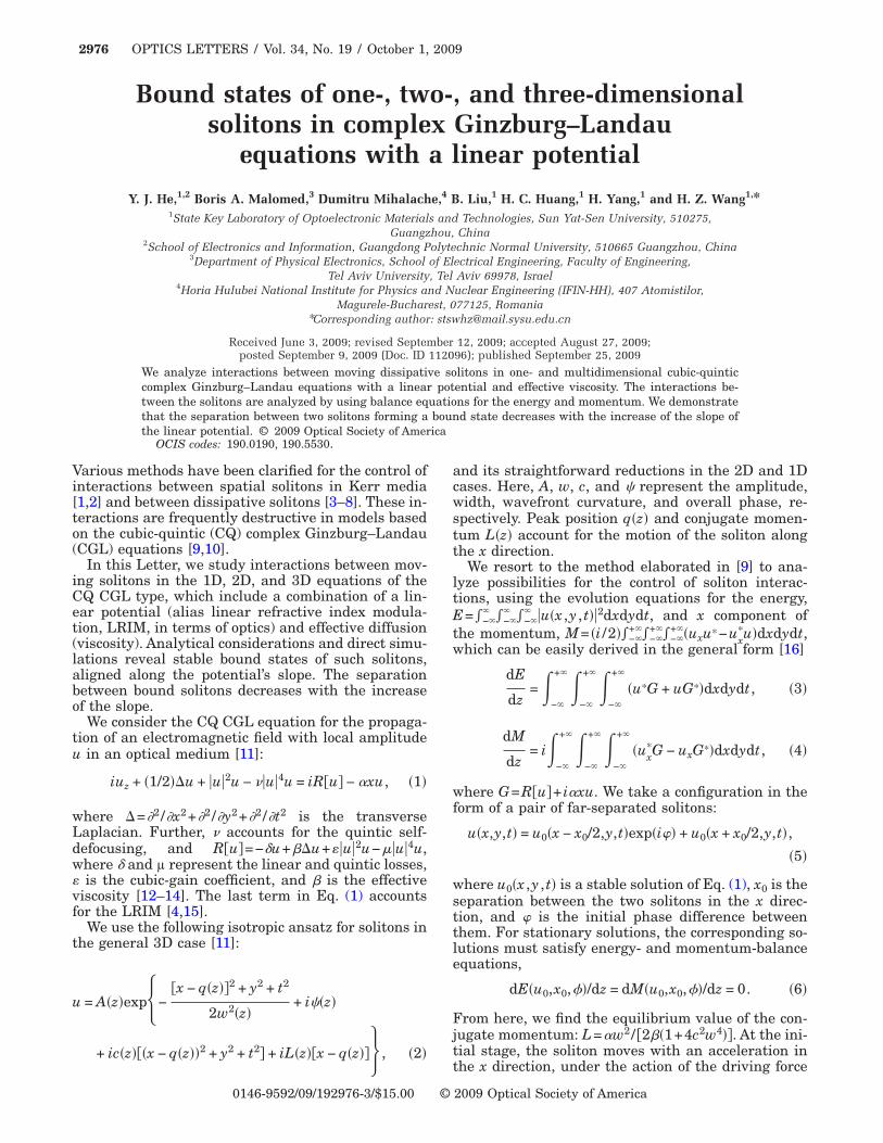
In the 1D case, the generic case may be repre-sented by ��0.5, ��0.5, µ�1, ��1.85, and ��0.115. The stable soliton solution was obtained inthe numerical form by the image-distance beampropagation method; see Fig. 1(a). Substituting two-soliton configuration (5) into Eq. (6), we represent thesolutions of Eq. (6) as curves in the plane �x0 ,�; seeFig. 1(b). Intersection points a and a� (for ��0), b(for ��0.06), and c (for ��0.12) correspond to two-soliton bound states. For ��0 the bound state with= ± /2 is found with the minimum separation�x0�min=9.4, as indicated by points a and a�, similarto bound states of temporal dissipative solitons[16,17]. The effect of the LRIM makes the phase dif-ference of the bound solitons slightly larger than /2,and it increases with the growth of � [Fig. 1(c)]. Theseparation between the bound solitons decreaseswith the increase of slope �, as seen in Fig. 1(d).Then, simulations of Eq. (1) yield the criticalvalue,�cr0.23, beyond which the 1D soliton loses itsstability. The curves shown in Fig. 1(b) are plotted ina limited range, 3.2w0�x0�11w0, as the linear-superposition approximation, Eq. (5), is not valid forsmall x0. Examples of direct simulations of Eq. (1) areshown in Figs. 1(e) and 1(f), which clearly demon-strate either the fusion of the solitons or the forma-tion of the bound state.

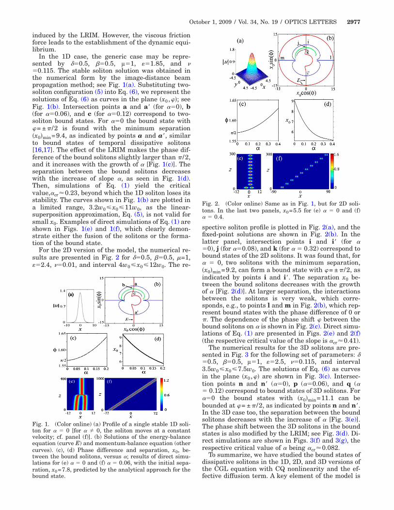
For the 2D version of the model, the numerical re-sults are presented in Fig. 2 for ��0.5, ��0.5, �=1,��2.4, ��0.01, and interval 4w0�x0�12w0. The re-

Fig. 1. (Color online) (a) Profile of a single stable 1D soli-ton for � � 0 [for � � 0, the soliton moves at a constantvelocity; cf. panel (f)]. (b) Solutions of the energy-balanceequation (curve E) and momentum-balance equation (othercurves). (c), (d) Phase difference and separation, x0, be-tween the bound solitons, versus �; results of direct simu-lations for (e) � � 0 and (f) � � 0.06, with the initial sepa-ration, x0=7.8, predicted by the analytical approach for the

bound state.

spective soliton profile is plotted in Fig. 2(a), and thefixed-point solutions are shown in Fig. 2(b). In thelatter panel, intersection points i and i� (for ��0), j (for ��0.08), and k (for � � 0.32) correspond tobound states of the 2D solitons. It was found that, for� � 0, two solitons with the minimum separation,�x0�min=9.2, can form a bound state with = ± /2, asindicated by points i and i�. The separation x0 be-tween the bound solitons decreases with the growthof � [Fig. 2(d)]. At larger separation, the interactionsbetween the solitons is very weak, which corre-sponds, e.g., to points l and m in Fig. 2(b), which rep-resent bound states with the phase difference of 0 or . The dependence of the phase shift between thebound solitons on � is shown in Fig. 2(c). Direct simu-lations of Eq. (1) are presented in Figs. 2(e) and 2(f)(the respective critical value of the slope is �cr0.41).

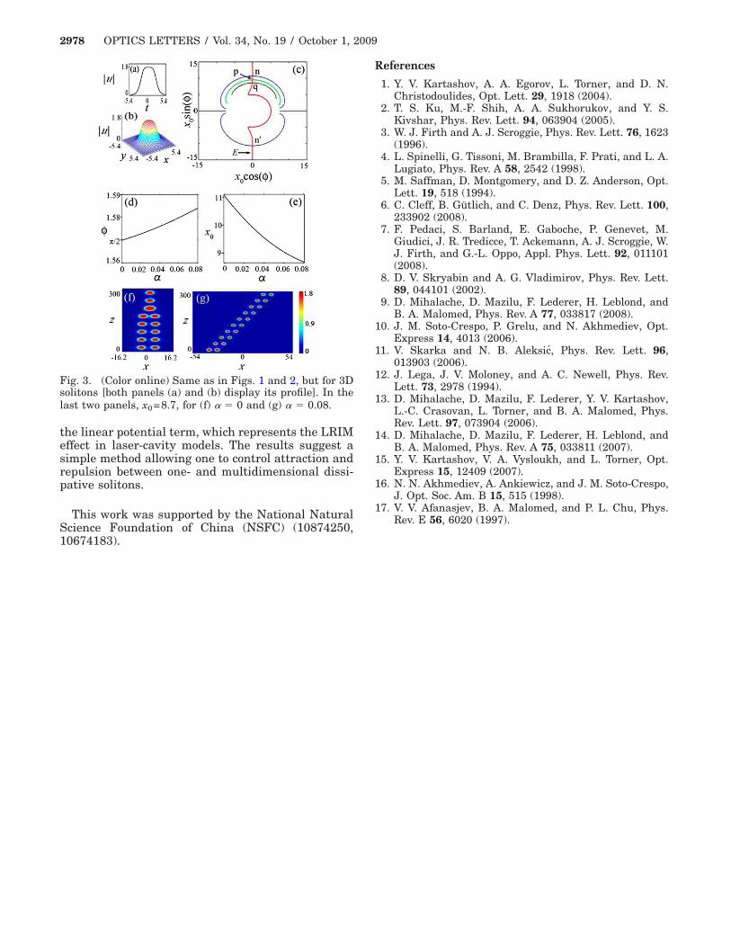
The numerical results for the 3D solitons are pre-sented in Fig. 3 for the following set of parameters: ��0.5, ��0.5, µ�1, ��2.5, ��0.115, and interval3.5w0�x0�7.5w0. The solutions of Eq. (6) as curvesin the plane �x0 ,� are shown in Fig. 3(c). Intersec-tion points n and n� (��0), p (��0.06), and q (�� 0.12) correspond to bound states of 3D solitons. For��0 the bound states with �x0�min=11.1 can bebounded at = ± /2, as indicated by points n and n�.In the 3D case too, the separation between the boundsolitons decreases with the increase of � [Fig. 3(e)].The phase shift between the 3D solitons in the boundstates is also modified by the LRIM; see Fig. 3(d). Di-rect simulations are shown in Figs. 3(f) and 3(g), therespective critical value of � being �cr0.082.

To summarize, we have studied the bound states ofdissipative solitons in the 1D, 2D, and 3D versions ofthe CGL equation with CQ nonlinearity and the ef-

Fig. 2. (Color online) Same as in Fig. 1, but for 2D soli-tons. In the last two panels, x0=5.5 for (e) � � 0 and (f)� � 0.4.

fective diffusion term. A key element of the model is

2978 OPTICS LETTERS / Vol. 34, No. 19 / October 1, 2009

the linear potential term, which represents the LRIMeffect in laser-cavity models. The results suggest asimple method allowing one to control attraction andrepulsion between one- and multidimensional dissi-pative solitons.

This work was supported by the National NaturalScience Foundation of China (NSFC) (10874250,10674183).

Fig. 3. (Color online) Same as in Figs. 1 and 2, but for 3Dsolitons [both panels (a) and (b) display its profile]. In thelast two panels, x0=8.7, for (f) � � 0 and (g) � � 0.08.

References

1. Y. V. Kartashov, A. A. Egorov, L. Torner, and D. N.Christodoulides, Opt. Lett. 29, 1918 (2004).

2. T. S. Ku, M.-F. Shih, A. A. Sukhorukov, and Y. S.Kivshar, Phys. Rev. Lett. 94, 063904 (2005).

3. W. J. Firth and A. J. Scroggie, Phys. Rev. Lett. 76, 1623(1996).

4. L. Spinelli, G. Tissoni, M. Brambilla, F. Prati, and L. A.Lugiato, Phys. Rev. A 58, 2542 (1998).

5. M. Saffman, D. Montgomery, and D. Z. Anderson, Opt.Lett. 19, 518 (1994).

6. C. Cleff, B. Gütlich, and C. Denz, Phys. Rev. Lett. 100,233902 (2008).

7. F. Pedaci, S. Barland, E. Gaboche, P. Genevet, M.Giudici, J. R. Tredicce, T. Ackemann, A. J. Scroggie, W.J. Firth, and G.-L. Oppo, Appl. Phys. Lett. 92, 011101(2008).

8. D. V. Skryabin and A. G. Vladimirov, Phys. Rev. Lett.89, 044101 (2002).

9. D. Mihalache, D. Mazilu, F. Lederer, H. Leblond, andB. A. Malomed, Phys. Rev. A 77, 033817 (2008).

10. J. M. Soto-Crespo, P. Grelu, and N. Akhmediev, Opt.Express 14, 4013 (2006).

11. V. Skarka and N. B. Aleksic, Phys. Rev. Lett. 96,013903 (2006).

12. J. Lega, J. V. Moloney, and A. C. Newell, Phys. Rev.Lett. 73, 2978 (1994).

13. D. Mihalache, D. Mazilu, F. Lederer, Y. V. Kartashov,L.-C. Crasovan, L. Torner, and B. A. Malomed, Phys.Rev. Lett. 97, 073904 (2006).

14. D. Mihalache, D. Mazilu, F. Lederer, H. Leblond, andB. A. Malomed, Phys. Rev. A 75, 033811 (2007).

15. Y. V. Kartashov, V. A. Vysloukh, and L. Torner, Opt.Express 15, 12409 (2007).

16. N. N. Akhmediev, A. Ankiewicz, and J. M. Soto-Crespo,J. Opt. Soc. Am. B 15, 515 (1998).

17. V. V. Afanasjev, B. A. Malomed, and P. L. Chu, Phys.Rev. E 56, 6020 (1997).