Project Number: ME-HXA-MG71

Bottling Line Splitter Design

A Major Qualifying Project Report

Submitted to the Faculty of the

WORCESTER POLYTECHNIC INSTITUTE

in partial fulfillment of the requirements for the

Degree of Bachelor of Science

in Mechanical Engineering

By

William Robinson Caruso James Saunders

___________________________________________

___________________________________________

Date: March 3rd, 2007

Approved:

____________________________________

Prof. Holly K. Ault Keywords:

1. Bottling 2. Machine Design 3. Beverage Production

i

Acknowledgements Special thanks to those persons without whom this project would not have been possible. Worcester Polytechnic Institute Professor Holly K. Ault Professor Henry Nowick James Phelan IGSD Professor Robert L. Norton E & J Gallo Wineries Mike Delikowski Laura Hoffman David Booth Loel Peters Brandon Abell Shawn Burns Jim Bellins Tim Phillipsen Juan Nevarez Others RPDG San Diego Rexell-Norcal Modesto

ii

Abstract E&J Gallo Winery in Modesto, CA has numerous high speed bottling lines where

it is necessary to split a single line of bottles into two lines. The current lane splitting mechanism uses multiple pneumatic actuators that require costly maintenance and cause excessive line downtime. A prototype mechanism utilizing a unique three-dimensional camoid design and single servo motion control was designed, fabricated using rapid prototyping methods, and tested. Preliminary tests results proved acceptable functionality. Shape optimization and long-term tests for reliability were recommended.

iii

ACKNOWLEDGEMENTS........................................................................................................... I

ABSTRACT .................................................................................................................................. II

LIST OF FIGURES..................................................................................................................VIII

LIST OF TABLES.........................................................................................................................X

LIST OF EQUATIONS .............................................................................................................. XI

CHAPTER 1.0 - INTRODUCTION ............................................................................................ 1

CHAPTER 2.0 - GOAL STATEMENT ...................................................................................... 3

CHAPTER 3.0 - TASK SPECIFICATIONS .............................................................................. 4

3.1 - ASSUMPTIONS......................................................................................................................... 4 3.2 - PERFORMANCE SPECIFICATIONS.......................................................................................... 4 3.3 - DESIGN SPECIFICATIONS ....................................................................................................... 4 3.4 - IDEAL CASES........................................................................................................................... 5

CHAPTER 4.0 - BACKGROUND............................................................................................... 6

4.1 - GALLO’S HIGH SPEED BOTTLING OPERATIONS.................................................................. 6 4.2 - E&J GALLO LINE 2 OVERVIEW............................................................................................ 6 4.3 - HEUFT REJECTION SYSTEM .................................................................................................. 7 4.3.1 - OVERVIEW ............................................................................................................................ 7 4.3.2 - MECHANISM COMPONENTS .................................................................................................. 8 4.3.3 - CONTROLS .......................................................................................................................... 10 4.4 - PLANT TOURS....................................................................................................................... 13 4.4.1 - WACHUSETT MICRO-BREWERY ......................................................................................... 13 4.4.2 - NORTHEASTERN REGIONAL ANHEUSER-BUSCH BREWERY............................................... 14 4.5 - OTHER HIGH SPEED LINE SPLIT SOLUTIONS .................................................................... 15 4.5.1 - PATENT RESEARCH............................................................................................................. 15 4.5.2 - OEM PRODUCTS................................................................................................................. 15 4.6 - RAPID PROTOTYPING........................................................................................................... 19 4.7 - SERVO MOTORS ................................................................................................................... 19

CHAPTER 5.0 - CAMOID DESIGN CONCEPTION............................................................. 20

5.1 - CAMOID GEOMETRY............................................................................................................ 22 5.1.1 - CAMOID CONCEPT .............................................................................................................. 22 5.1.2 - CAMOID INSPIRATION......................................................................................................... 22

iv

5.1.3 - CAMOID DESIGN ................................................................................................................. 23 5.2 - ACTUATION DESIGN............................................................................................................. 29 5.2.1 - WHY USE A SERVO?............................................................................................................ 29 5.2.2 - CHOOSING A SERVO............................................................................................................ 30 5.2.3 - SIZING A SERVO.................................................................................................................. 30 5.2.4 - CONTROLLING THE SERVO ................................................................................................. 31 5.2.5 - ACTUATION DESIGN CONCLUSIONS ................................................................................... 32 5.3 - DESIGN CONCEPT SUMMARY ............................................................................................... 32

CHAPTER 6.0 - METHODOLOGY ......................................................................................... 33

6.1 - ASSUMPTIONS....................................................................................................................... 33 6.1.1 - LINE 2 PROPERTIES............................................................................................................. 33 6.1.2 - HEUFT LANER..................................................................................................................... 33 6.2 - DATA COLLECTION AND ANALYSIS .................................................................................... 34 6.2.1 - HEUFT ANALYSIS ............................................................................................................... 34 6.2.2 - CONTOUR DESIGN AND ANALYSIS ..................................................................................... 34 6.2.3 - CHOOSING CONTOUR.......................................................................................................... 35 6.3 - CAMOID GEOMETRY DESIGN.............................................................................................. 36 6.3.1 - MANUFACTURE................................................................................................................... 36 6.4 - ACTUATION DESIGN............................................................................................................. 38 6.4.1 - SIZING A SERVO.................................................................................................................. 38 6.5.2 - CONTROLLING THE SERVO ................................................................................................. 39 6.5.3 - STRESS ANALYSIS............................................................................................................... 41 6.5.4 - FATIGUE STRESS ANALYSIS ............................................................................................... 41 6.6 - PART GATHERING ................................................................................................................ 41 6.7 - CHASSIS DESIGN................................................................................................................... 41 6.7.1 - MATERIAL .......................................................................................................................... 42 6.7.2 - COMPONENT LAYOUT......................................................................................................... 42 6.7.3 - IMPLEMENTATION ON LINE ................................................................................................ 43 6.7.4 - MANUFACTURABILITY ....................................................................................................... 44 6.8 - DRIVE SYSTEM ..................................................................................................................... 44 6.9 - MECHANISM ASSEMBLY ...................................................................................................... 45 6.10 - IMPLEMENTATION.............................................................................................................. 45 6.11 - TESTING .............................................................................................................................. 46

CHAPTER 7.0 - CAMOID LANER DETAILED DESIGN .................................................... 47

7.1 - CAMOID GEOMETRY DESIGN.............................................................................................. 47 7.1.1 - ITERATIVE DESIGN ............................................................................................................. 47 7.1.2 - GEOMETRY FINAL VALUES ................................................................................................ 52 7.1.3 - GEOMETRY CONSTRUCTION............................................................................................... 52 7.2 - CAMOID PROTOTYPE........................................................................................................... 52 7.3 - ACTUATION DESIGN............................................................................................................. 53 7.3.1 - SERVO SIZING..................................................................................................................... 53 7.3.2 - SERVO SYSTEM................................................................................................................... 53 7.3.3 - CONTROL LOGIC CONCEPT................................................................................................. 57 7.3.4 - DRIVE TRAIN SPECS ........................................................................................................... 57 7.3.5 - TIMING................................................................................................................................ 57

v

7.4 - MOTION ANALYSIS............................................................................................................... 60 7.4.1 - CAM EXTENSION................................................................................................................. 60 7.5 - CHASSIS DESIGN DETAILS ................................................................................................... 60 7.5.1 - MATERIAL CHOICE ............................................................................................................. 62 7.5.2 - LAYOUT .............................................................................................................................. 62 7.5.3 - TOLERANCES ...................................................................................................................... 63 7.5.4 - FASTENERS ......................................................................................................................... 64 7.5.5 - BEARINGS ........................................................................................................................... 64 7.6 - DRIVE DESIGN DETAILS ...................................................................................................... 64 7.6.1 - RECOMMENDATION ............................................................................................................ 66 7.6.2 - CLAIMED BENEFITS ............................................................................................................ 66 7.6.3 - CHASSIS LAYOUT ............................................................................................................... 66 7.6.4 - DRIVE RATIO ...................................................................................................................... 66 7.6.5 - AVAILABILITY .................................................................................................................... 66 7.6.6 - BELT TENSIONER ................................................................................................................ 66 7.7 - FULL ASSEMBLY................................................................................................................... 68 7.8 - MECHANISM ASSEMBLY ...................................................................................................... 69 7.8.1 - CAMOID POSITION ON SHAFT ............................................................................................. 69 7.8.2 - CAMOID SHAFT ALIGNMENT .............................................................................................. 69 7.8.3 - SERVO INSTALLATION ........................................................................................................ 70 7.8.4 - SPROCKET POSITION........................................................................................................... 70 7.8.5 - BELT TENSIONING .............................................................................................................. 70 7.8.6 - INITIAL MOTION TEST ........................................................................................................ 71 7.9 - IMPLEMENTATION................................................................................................................ 71

CHAPTER 8.0 - DATA COLLECTION AND ANALYSIS .................................................... 72

8.1 - BOTTLE DYNAMIC ANALYSIS.............................................................................................. 72 8.1.1 - FRICTION TEST ................................................................................................................... 72 8.1.2 - CENTER OF GRAVITY TEST................................................................................................. 72 8.1.3 - NECK STRENGTH TEST ....................................................................................................... 73 8.2 - CAM PROFILE DESIGN AND ANALYSIS ............................................................................... 73 8.2.1 - CONSTRAINTS ..................................................................................................................... 74 8.2.2 - KINEMATIC ANALYSIS........................................................................................................ 75 8.2.3 - FORCE ANALYSIS................................................................................................................ 80 8.2.4 - MOMENT ANALYSIS ........................................................................................................... 82 8.3 - TRAJECTORY TEST .............................................................................................................. 83 8.4 - CHOOSING A CONTOUR ....................................................................................................... 84 8.4.1 - ACCEPTABLE FINAL VELOCITY .......................................................................................... 84 8.4.2 - MINIMIZING MAXIMUM ACCELERATION ........................................................................... 84 8.4.3 - MINIMIZING JERK ............................................................................................................... 84 8.4.4 - MINIMIZING FORCE ............................................................................................................ 84 8.4.5 - MINIMIZING MOMENT ........................................................................................................ 84 8.5 - TORQUE REQUIREMENTS .................................................................................................... 84 8.5.1 - OPERATING ROTATIONAL VELOCITY ................................................................................. 84 8.5.2 - ANGULAR ACCELERATION ................................................................................................. 85 8.5.3 - TORQUE REQUIRED............................................................................................................. 86 8.6 - STRESS ANALYSIS................................................................................................................. 87 8.7 - FATIGUE STRESS ANALYSIS ................................................................................................ 89

vi

CHAPTER 9.0 - PROTOTYPE TESTING............................................................................... 91

9.1 - MATERIALS........................................................................................................................... 91 9.2 - OBJECTIVE............................................................................................................................ 91 9.3 - VARIABLES ........................................................................................................................... 91 9.4 - SETUP SAFETY PRECAUTION............................................................................................... 91 9.5 - SETUP .................................................................................................................................... 92 9.5.1 - BOTTLE TEST BATCHES...................................................................................................... 92 9.5.2 - TEST LOOP SPEED............................................................................................................... 93 9.5.3 - PHOTOEYE PLACEMENT...................................................................................................... 93 9.5.4 - ELECTRONIC ATTACHMENT ............................................................................................... 93 9.6 - PROCEDURE SAFETY PRECAUTION..................................................................................... 94 9.7 - PROCEDURE.......................................................................................................................... 94 9.7.1 - DATA RECORDING .............................................................................................................. 94

CHAPTER 10.0 - TEST RESULTS........................................................................................... 95

10.1 - TESTING LIMITATIONS ...................................................................................................... 95 10.1.1 - LINE ENCODER ................................................................................................................. 96 10.1.2 - VARIABLE LINE SPEED ..................................................................................................... 96 10.1.3 - CONVEYOR CONDITION .................................................................................................... 96 10.1.4 - LINE SPEED....................................................................................................................... 96 10.2 - PRELIMINARY TESTING ..................................................................................................... 96 10.3 - RESULTS TABLE ................................................................................................................. 98 10.3.1 - MINIMUM BOTTLE SPACING: EXTENSION ........................................................................ 99 10.3.2 - MINIMUM BOTTLE SPACING: RETRACTION...................................................................... 99 10.3.3 - MAGNITUDE OF DISPLACEMENT ...................................................................................... 99 10.3.4 – PHOTOEYE PLACEMENT................................................................................................... 99 10.4 - MECHANISM OBSERVATIONS .......................................................................................... 100 10.5 - TEST RESULTS CONCLUSIONS......................................................................................... 100

CHAPTER 11.0 - COST COMPARISON............................................................................... 101

CHAPTER 12.0 - RECOMMENDATIONS ........................................................................... 102

12.1 - LINE SPEED TESTING ....................................................................................................... 102 12.2 - BOTTLE TESTING ............................................................................................................. 102 12.3 - ENDURANCE TESTING...................................................................................................... 102 12.4 - PART ACQUISITION .......................................................................................................... 102 12.5 - PROGRAM OPTIMIZATION............................................................................................... 102 12.6 - GEOMETRY OPTIMIZATION ............................................................................................ 102

CHAPTER 13.0 - CONCLUSIONS......................................................................................... 103

REFERENCES .......................................................................................................................... 104

APPENDICES ........................................................................................................................... 105

vii

APPENDIX A - RELEVANT PATENTS.......................................................................................... 106 APPENDIX B - RAPID PROTOTYPING QUOTES.......................................................................... 113 APPENDIX C - BILL OF MATERIALS .......................................................................................... 114 APPENDIX D - MOTION ANALYZER INPUT VALUES................................................................. 118 APPENDIX E - SERVO DETAILS.................................................................................................. 120 APPENDIX F - SERVO DRIVER DETAILS.................................................................................... 122 APPENDIX G - CHASSIS DRAWINGS........................................................................................... 125 APPENDIX H - GOODYEAR EAGLE PD POWER TRANSMISSION .............................................. 133 APPENDIX I - BOTTLE TESTS..................................................................................................... 141 I.1 - CENTER OF GRAVITY TEST .................................................................................................. 141 I.2 - COEFFICIENT OF STATIC FRICTION TEST ............................................................................. 145 I.3 - BOTTLE NECK FAILURE TEST .............................................................................................. 147 I.3 - BOTTLE NECK FAILURE TEST .............................................................................................. 148 APPENDIX J - RAPID PROTOTYPING METHODS ....................................................................... 150 J.1 - STEREOLITHOGRAPHY (SLA)............................................................................................... 150 J.2 - FUSED DEPOSITION MODELING (FDM) ............................................................................... 150 J.2 - FUSED DEPOSITION MODELING (FDM) ............................................................................... 151 J.3 - SELECTIVE LASER SINTERING (SLS) ................................................................................... 151 J.4 - ELECTRON BEAM MELTING (EBM)..................................................................................... 151 APPENDIX K – TEST DATA TABLE ............................................................................................ 152 APPENDIX M - DETAILED MATHEMATICS................................................................................ 153

viii

List of Figures Figure 1: Patent 4,369,873 Concept.................................................................................... 8 Figure 2 (left): Line 2 Heuft Delta-FW On Position........................................................... 8 Figure 3 (right): Line 2 Heuft Delta-FW Off Position........................................................ 8 Figure 4: Cylinder Layout (top view) ................................................................................. 9 Figure 5 (left): Segments in Off Position (top view) .......................................................... 9 Figure 6 (right): Contour in On Position............................................................................. 9 Figure 7: Segment Depth and Bristles .............................................................................. 10 Figure 8: Segment Close-up (top view). Note bristles on end of each segment. .............. 10 Figure 9: Heuft operation off to on switch........................................................................ 12 Figure 10: Wachusett Lane Splitter .................................................................................. 14 Figure 11: Heuft Delta-K Unit.......................................................................................... 16 Figure 12: Heuft Flip Rejecter .......................................................................................... 17 Figure 14: KHS Waveform............................................................................................... 18 Figure 15: Top view of KHS Waveform .......................................................................... 18 Figure 17: Camoid Laner .................................................................................................. 20 Figure 18: Camoid Extension ........................................................................................... 21 Figure 19: Heuft Delta-K Bottle Rejecter......................................................................... 22 Figure 20: Camoid Laner Shape ....................................................................................... 23 Figure 21: Geometry Terminology ................................................................................... 24 Figure 22: Cam Segment Construction............................................................................. 25 Figure 23: Segmented Camoid.......................................................................................... 26 Figure 24: Cam segment phase shifting............................................................................ 28 Figure 25: Sections of Continuous Contour...................................................................... 28 Figure 26: Heuft Contour and Equation............................................................................ 34 Figure 27: Component Layout .......................................................................................... 43 Figure 28: Heuft Attachment to Line................................................................................ 44 Figure 29: Test Loop......................................................................................................... 46 Figure 30: Geometric Elements ........................................................................................ 48 Figure 38: Model vs. Rapid prototype .............................................................................. 53 Figure 39: Servo Control Schematic................................................................................. 54 Figure 40: Servo Motor..................................................................................................... 55 Figure 41: Timing Diagram Example ............................................................................... 58 Figure 42: Top View of Cam Extension ........................................................................... 60 Figure 43: Chassis Assembly View .................................................................................. 61 Figure 44: Chassis Exploded View................................................................................... 62 Figure 45: Important Toleranced Dimensions .................................................................. 64 Figure 46: Goodyear Eagle Pd Power Transmission ........................................................ 65 Figure 47: Lovejoy Belt Tensioner with smooth idler pulley........................................... 67 Figure 48: Full CAD Assembly ........................................................................................ 68 Figure 49: Full Assembly.................................................................................................. 69 Figure 50: Tensioning Diagram........................................................................................ 70 Figure 54: Contour of Each Cam Program ....................................................................... 76 Figure 55: Displacement Difference, Heuft vs. Cam Programs ....................................... 77 Figure 56: Bottle Transverse Velocity.............................................................................. 78

ix

Figure 57: Bottle Transverse Acceleration ....................................................................... 78 Figure 58: Bottle Transverse Jerk ..................................................................................... 79 Figure 59: Bottle Free Body Diagram .............................................................................. 80 Figure 60: Force on Bottle ................................................................................................ 81 Figure 61: Induced Moment on Bottles ............................................................................ 82 Figure 62: Bottle Trajectories ........................................................................................... 83 Figure 63: Spin-up time vs. Buffer Angle ........................................................................ 85 Figure 64: Acceleration vs. Spin-Up Time ....................................................................... 86 Figure 65: Servo Torque Required vs. Spin-Up Time...................................................... 87 Figure 66: Test loop.......................................................................................................... 92 Figure 67: Electronics Board ............................................................................................ 93 Figure 68: Final Mechanism Cycle Sequence .................................................................. 95 Figure 69: Photoeye Placement ........................................................................................ 99 Figure 70: Patent 4,986,407 ............................................................................................ 106 Figure 71: Patent 4,643,291 ............................................................................................ 107 Figure 72: Patent 4,321,994 ............................................................................................ 108 Figure 73: Patent 4,369,873 ............................................................................................ 109 Figure 74: Patent 6588575.............................................................................................. 110 Figure 75: Patent 6,822,181 ............................................................................................ 111 Figure 76: Patent 3,791,518 ............................................................................................ 112 Figure 77: Servo Overview............................................................................................. 120 Figure 78: Driver Details and Benefits ........................................................................... 122 Figure 79: Driver Specifications..................................................................................... 123 Figure 80: Driver Specifications..................................................................................... 124 Figure 81: Belt Nomenclature......................................................................................... 133 Figure 82: Eagle Pd Belt Product Numbers.................................................................... 134 Figure 83: Sprocket Nomenclature ................................................................................. 135 Figure 84: Eagle Pd White Sprockets ............................................................................. 136 Figure 85: Belt Nomenclature......................................................................................... 137 Figure 86: Eagle Pd Belt Product Numbers.................................................................... 138 Figure 87: Sprocket Nomenclature ................................................................................. 139 Figure 88: Eagle Pd White Sprockets ............................................................................. 140 Figure 89: Center of Gravity Experiment ....................................................................... 142 Figure 90: Free Body Diagram ....................................................................................... 143 Figure 91: Free Body Diagram ..........................................Error! Bookmark not defined. Figure 93: Coefficient of Static Friction Experiment ..................................................... 145 Figure 94: Free Body Diagram ....................................................................................... 146 Figure 97: Bottle Neck Failure Experiment.................................................................... 148 Figure 98: Free Body Diagram ....................................................................................... 149

x

List of Tables Table 1: Manufacturing Method Comparison................................................................... 37 Table 2: Rapid Prototyping Method Comparison............................................................. 37 Table 3: Material Comparison .......................................................................................... 42 Table 4: Camoid Geometry Final Values ......................................................................... 52 Table 5: Servo Motor and Gearbox Overview Specs ....................................................... 56 Table 6: Driver Overview Specs....................................................................................... 56 Table 7: Tolerance Reasons .............................................................................................. 63 Table 8: Belt Used ............................................................................................................ 65 Table 9: Sprockets Used ................................................................................................... 65 Table 10: Cam Program Constraints................................................................................. 75 Table 11: Graphic Color Scheme...................................................................................... 76 Table 12: Maximum Kinematic Values............................................................................ 80 Table 13: Maximum Force Analysis Values .................................................................... 83 Table 14: Time Data ......................................................................................................... 85 Table 15: Keyway Stress Analysis ................................................................................... 88 Table 16: Shaft Stress Analysis ........................................................................................ 89 Table 17: Shaft Fatigue Analysis...................................................................................... 89 Table 18: Keyway Stress Concentration Analysis............................................................ 90 Table 19: Test Results....................................................................................................... 98 Table 20: Cost Comparison ............................................................................................ 101 Table 21: Full Bill of Materials ...................................................................................... 115 Table 22: Bill of Materials with Piggy Backed Electronics ........................................... 117 Table 23: Axis Setup Tab ............................................................................................... 118 Table 24: Cycle Profile Tab............................................................................................ 118 Table 25: Mechanism Tab .............................................................................................. 119 Table 26: Transmission Stages Tab ................................................................................ 119 Table 27: Data Recording Table ..................................................................................... 152

xi

List of Equations Equation 1: Bottle and Laner Contact Time ..................................................................... 85 Equation 2: Operational Rotational Velocity.................................................................... 85 Equation 3: Worst Case Scenario Time Between Two Bottles ........................................ 85 Equation 4: Acceleration Function ................................................................................... 86 Equation 5: Torque Function ............................................................................................ 86 Equation 6: Shear Force at Key ........................................................................................ 88 Equation 7: Keyway Average Shear Stress ...................................................................... 88 Equation 8: Safety Factor.................................................................................................. 88 Equation 9: Area of Key ................................................................................................... 88 Equation 10: Required Torque.......................................................................................... 88 Equation 11: Shaft Torsional Deflection .......................................................................... 89 Equation 12: Shaft Shear Stress due to Torsion................................................................ 89 Equation 13: Shaft Polar Moment of Inertia..................................................................... 89 Equation 14: Corrected Fatigue Function ......................................................................... 89 Equation 15: Safety Factor................................................................................................ 89 Equation 16: Fatigue Stress Concentration Factor............................................................ 90 Equation 17: Shear Stress Concentration due to Torsion ................................................. 90 Equation 18: Safety Factor................................................................................................ 90

1

Chapter 1.0 - Introduction E&J Gallo Winery is one of the largest winemaking operations in the world. Founded in 1933 by Ernest and Julio Gallo, the Gallo Winery is still a family business and since has expanded to the global market. Currently, Gallo Winery employs over 4600 people and retails wines throughout the United States and over 90 foreign countries. Grapes used are from vineyards spanning California’s most important wine-producing regions and Gallo runs operations in sites across Sonoma County including Modesto, Monterey and Napa Valley. The diverse product line of Gallo Winery ranges from fine table and sparkling wines, to distilled wine-based spirits and beverages (E&J Gallo, 2003). This project is conducted in E&J Gallo’s Modesto site and focuses on 750mL bottled wine production, specifically on Line 2. At full production Line 2 fills and packages at up to 400 bottles per minute, running 16 hour shifts, seven days per week. The limiting factor in the production speed of the line is the packaging process. In attempt to maximize the efficiency of the line, Gallo employs two parallel packaging lines resulting in the need for a lane split from single file to two independent lanes between the bottle filler and the packing equipment. Gallo is experiencing expensive maintenance issues with the mechanism which splits the lanes. The current system is manufactured by Heuft. The manufacturer’s recommendation for the mechanism states its function to be a single bottle rejecter. However, in Line 2 the Heuft rejecter functions as a high speed lane splitter. The difference is in the number of cycles per unit time. As a rejecter, the mechanism might actuate several dozen times per shift, but as a dedicated lane splitter, it fires several thousand times per shift. This results in a significant deterioration of performance in a relatively short period of time, and thus requires maintenance or replacement often enough to cause concern. Furthermore, as performance degrades, the chance of bottle damage or bottle tipping increases which can cause costly delays in production.

In order to reduce the maintenance cost and production delays associated with the Heuft laning mechanism, Gallo proposed a redesign of the system. Within the proposal, Gallo specified certain criteria that the redesign must follow. The new system must reduce maintenance costs, must fit within the existing footprint, and not damage bottles. The new system must not be a safety hazard. And the system must ideally be replicable on other lines with different size and shape bottles.

This project focuses specifically on the redesign of the Line 2 Heuft system. Through problem identification, research, ideation, analysis, modeling, prototypes and implementation, this project will propose a solution to the problems experienced with the current system. The following report will explain the details of design, implementation, experimentation and results of a unique prototype lane splitting mechanism.

The chapters present information in parallel structures with each successive chapter’s investigation driving progressively deeper in detail. After discussing relevant background information, the design process is explained in detail over chapters 5-7. Chapter 5 introduces the idea explaining terminology and design basics. Chapter 6 describes the methodology used to create that design. Chapter 7 describes the detailed design process and gives all values in the final design. Chapter 8 details all important calculations conducted. Chapters 9 and 10 describe the experimental process; procedure

2

and results. Chapter 11 concludes the project with a cost analysis. Conclusions and recommendations are discussed in the final chapters. This structure will tend to a variety of audiences and allow quicker reference for those familiar with the project and detailed step-by-step explanation for those who are not.

3

Chapter 2.0 - Goal Statement The aim of this project is to design a means of splitting one high-speed single-file

line of bottles into two independent single-file lines. Alternatively, the existing mechanism may be improved to reduce maintenance costs and upkeep.

4

Chapter 3.0 - Task Specifications

This chapter outlines the design specifications that must be met in order to claim a successful solution.

3.1 - Assumptions

This specification list was compiled assuming 750mL bottles traveling at 400 bottles/min with a space of one bottle diameter between each bottle. We assume a worst case operation of 16 hours/day, 365 days/year, and a lane switching frequency of 10 bottles per lane. A full cycle requires the mechanism to transition from ‘off’ to ‘on’ and back to ‘off’, allowing 20 bottles to pass. This adds up to nearly 7 million cycles per year.

3.2 - Performance Specifications

The Laning Mechanism Must:

• NOT cost more than $20,000 in parts, or more than $10,000 in installation. • Reduce maintenance costs from the current $10,000/year. • NOT damage or scuff bottles or labels. • Allow for either packer lane to be utilized independently.

o This would require the mechanism to remain in either the ‘on’ or ‘off’ position for extended time if necessary.

• Accommodate for variable line speeds. • Be frequency adjustable. This refers to the number of bottles to pass per cycle. • Follow food handling guidelines and regulations. • Be actuated without interfering with bottles.

o This means that any mechanism should be able to switch from ‘on’ to ‘off’ without a bottle being influenced in this transition. The likely way to accomplish this is to have the actuation take place in the space between bottles as they pass. Our estimate of this time is 0.064 seconds.

• Be able to redirect bottles moving with a kinetic energy of 0.5-1.0 Joules. • Be sustainable with routine maintenance. • Fit in the existing system’s footprint. • NOT cause downed bottles. • NOT present a safety hazard to employees during operation or maintenance.

3.3 - Design Specifications

• The frequency adjustability should be done by counting bottles (as opposed to a timed action).

• Routine maintenance should be accommodated in the design. Special tools or parts should not be necessary to service and maintain the mechanism.

• Tipping must be controlled, both induced (through the mechanism’s workings) and accidental.

5

3.4 - Ideal Cases

• The design is applicable in various lines with various bottle types. • The design has a lifespan of 5 years (35 million cycles).

6

Chapter 4.0 - Background Maintenance issues with a high speed lane splitter system on line 2 are causing unneeded expenditures. This background chapter will offer insight into several of the base issues that underlie a high speed lane splitting mechanism. Additional background information regarding various components utilized in the design is also presented. The topics of discussion will be:

• High speed bottling process • Overview of Gallo’s line 2 bottle laning section • Examples of other bottling facilities • Heuft Bottle Rejection system • Rapid Prototyping • Servo Motors • Commercially Available High Speed Lane Splitters • Patent Research

4.1 - Gallo’s High Speed Bottling Operations Gallo is one of the largest wineries in the world selling over 67 million cases of wine annually, 1/3 of which is shipped to international markets. Most of Gallo’s bottling operations are handled in the Modesto bottling plant. The Modesto bottling plant is supplied by millions of gallons of stored wine which is fed to 17 bottling lines. Each of the lines is designed to accommodate a certain type of container. Gallo’s container lineup includes Bag-in-Box; 5L and 3L jugs; 1.5L, 750mL, 375mL and 187mL bottles. A variety of different products could fill any of the bottles including table wine, sparkling wine, wine cooler beverages and ciders. The lines run at different speeds depending on bottle size varying from 100 bottles per minute for jugs to up to 1000 bottles per minute for the wine beverages. The bottling lines are almost completely automated, with a small team of operators, inspectors and mechanics for each line. Occasional problems can occur such as broken or tipped bottles, filling mistakes, labeling mistakes, or misfeeds on caps or corks. The line incorporates a series of inspection and rejection systems to discard any problematic bottles; however operators are still present to ensure smooth operation. The rejection systems can be found on almost every line. These rejection systems use the same mechanism as the lane splitters, which also can be found on most of the lines. The rejection systems and lane splitters are essential to the company to maintain production quality and speed.

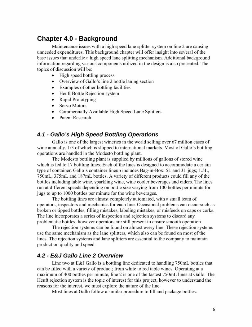
4.2 - E&J Gallo Line 2 Overview Line two at E&J Gallo is a bottling line dedicated to handling 750mL bottles that can be filled with a variety of product; from white to red table wines. Operating at a maximum of 400 bottles per minute, line 2 is one of the fastest 750mL lines at Gallo. The Heuft rejection system is the topic of interest for this project, however to understand the reasons for the interest, we must explore the nature of the line. Most lines at Gallo follow a similar procedure to fill and package bottles:

7

1. Empty bottles arrive up-side-down in cases that are stacked on pallets 2. The rows of cases are stripped from the pallet and fed single file on a conveyor 3. The cases are tipped up-side-down to remove empty bottles 4. Cases and bottles are separated 5. Bottles are rinsed 6. Bottles are filled and corked 7. Bottles are x-ray inspected 8. Bottles are dried 9. Bottles are capped 10. Bottles are labeled 11. Bottles are cased and packaged 12. Cases are palletized and stored

The point of interest is after step 7, which is where rejection and lane splitting

occurs. The reason for the lane split is because the packaging machine is not capable of the line speed of the filler. In order to compensate for the slower packaging machine, Gallo employs two machines.

The method by which the bottles are divided into separate lanes is the Heuft Rejection system. This system is designed to be used as a single bottle rejection system, however is used on many of the Gallo lines as a dedicated lane splitter. The system causes a significant amount of maintenance costs because of the number of cycles it must endure. A rejecter may actuate several dozen times per day, while a dedicated laner actuates thousands of times per day. The system is not designed for this high number of cycles and thus experiences malfunctions and wear in a relatively short period of time.

4.3 - Heuft Rejection System

4.3.1 - Overview The Heuft Rejection System is based on a design invented by Bernhard Heuft and

is currently manufactured and distributed by Heuft Systemtechnik Gmbh of Germany. Founded in 1979, the company has based its business on innovation and unusual ideas that have since become industry standards. Today Heuft is represented all over the world with 20 subsidiary company locations on 5 continents (Heuft, 2007). The Heuft rejecter initial concept was filed by Bernhard Heuft for U.S. patent number 4,369,873 filed January 10, 1979 under the title Apparatus for Laterally Deflecting Articles. This concept was later improved upon in patent number 4,321,994 on April 21, 1980 under the title Means for Laterally Deflecting Articles from a Path of Travel. Since conception, the system has undergone minor changes to accommodate for modern production speeds, but the system has remained largely the same as the original concept. This patent is documented in Appendix A. The Heuft rejecter system used by Gallo Winery is named Heuft Delta-FW 16 and is boasted by the Heuft Company as a “robust, all around system for speed of up to 150,000 containers per hour [2500 containers/min]” (Heuft, 2007). While its primary purpose is to single out a container for rejection, Heuft states it can also be used for the “removal of fallen containers and foreign objects” (Heuft, 2007).

8

4.3.2 - Mechanism Components The system is comprised of 16 segments that are linearly actuated transversely

across the conveyor in front of the containers’ path of travel. Figure 1 shows a top view of the mechanism. Notice the segments’ independently controlled actuation and how only a single bottle is diverted while the others are not manipulated. The concept behind the design ensures that the bottles are diverted in a gradual manner to reduce the risk of tipping.

Figure 1: Patent 4,369,873 Concept1

Figure 2 (left): Line 2 Heuft Delta-FW On Position Figure 3 (right): Line 2 Heuft Delta-FW Off Position

The Heuft Delta-FW 16 is actuated by a means of 16 pneumatic cylinders ranging in cylinder body size and has adjustable stroke lengths. Each of the 16 cylinders is

1 Free Patents Online. Patent Analytics and Patent Searching. Retrieved January 8th, 2007. from

www.freepatentsonline.com.

9

controlled individually by an electronic solenoid valve. Note that Gallo uses only 12 of the 16 cylinders (Figure 2).

The 16 cylinders range from 45mm to 155mm in length and have an adjustable stroke length via a threaded piston rod and stopper nut. The strokes are adjustable using ordinary hexagonal sockets. The piston rod includes a rubber shock absorber between the cylinder and the stopper nut to decrease noise as well as wear and fatigue during actuation.

Figure 4: Cylinder Layout (top view) Attached to each piston rod is a plastic segment by which the bottles are diverted as seen in Figure 2. Each segment is approximately the same width. When all pistons are in the fully “off” position, the bottles are not diverted and continue on a neutral default path (Figure 2 and Figure 5). When the all pistons are actuated in the fully “on” position, the segments are arranged in a curved contour. The contour of each segment is linear, as shown in Figure 8. However the stroke lengths of each piston are such that the array forms the non-linear contour seen in Figure 6. Also each segment is progressively longer than the previous segment to aid in the horizontal translation.

Figure 5 (left): Segments in Off Position (top view) Figure 6 (right): Contour in On Position The segments are approximately 4 inches deep and have a row of bristles that act as a cushion for the bottle to limit impact and bottle scuffing ( Figure 7). The bristles are

10

approximately ¼ inch in length. In addition to bottle cushioning, the bristles also act as a buffer for any irregularities in segment spacing or piston actuation length.

Figure 7: Segment Depth and Bristles

Figure 8: Segment Close-up (top view). Note bristles on end of each segment.

4.3.3 - Controls The timing of the system is the most crucial element for the successful operation

of the system. To completely avoid the chance of tipped bottles, the basic concept of the

11

design is centered on single point guidance of a bottle. In essence, the timing of the firing sequence is such that the contour is laid out in front of a single container so that the bottle directly in front of the target bottle is not diverted and every bottle after the target is diverted. For single bottle diversion, the segments are retracted immediately after the target bottle has passed.

4.3.3.1 - Data Input In order to start the firing sequence correctly, the position of the bottles on the line must be recorded. This is accomplished by an electronic counting device directly before the rejecter. In order to fire the pistons at the correct time interval after the initial piston, the line speed must be recorded. Coupled to the rejecter’s control system is an encoder on the conveyor which records the line speed and bottle position. With these data known, the firing sequence can be timed correctly to avoid bottle tipping (Heuft USA, Inc.).

4.3.3.2 - “Off” to “On” Switch The first piston (shortest stroke) is always the first piston to fire. This must occur between the target bottle and the bottle directly in front of the target. Depending on the line speed, the pistons will continue to fire between these same two bottles. This insures that the diversion of the bottle is caused by a passive contour, i.e. the bottle will not be “punched” or pushed by an actuating piston. If a punch occurs, the bottle could accelerate laterally into the opposite side and cause an unwanted impact or tip. Once the pistons are all actuated, they remain in this position for a predetermined number of bottles to pass.

Figure 9 shows the firing sequence of the Heuft’s pistons. The bottles are highlighted for visualization. Note that the direction of travel is downward. The rejection system is on the right side of each photo.

12

Figure 9: Heuft operation off to on switch

A. Bottle 1 passes by the off segments. Bottle 2 approaches. B. Both Bottle 1 and Bottle 2 are passing the off segments. C. Bottle 1 continues to Lane 1. Bottle 2 is still passing the off segments. D-F. The segments begin to fire. Bottle 3 enters the beginning of the splitter. Bottle

3 is riding the on segments while Bottle 2 is riding the off segments simultaneously.

G. Bottle 2 continues to Lane 1. Bottle 3 is riding the on segments. H-I. Bottle 3 continues to Lane 2.

4.3.3.3 - “On” to “Off” Switch Again, the first piston is the first to fire and occurs between the target bottle and bottle directly in front of the target bottle. The sequence firing is the same as the “off” to “on” switch; however the bottle in front of the target bottle follows the contour, while the target bottle follows the default neutral path.

13

The system is designed to be able to single out one bottle from a stream without disrupting the rest of the stream by laying out a path in front of a single target bottle.

Malfunctions associated with the Heuft system occur most often with the pneumatic actuators. The seals wear and the actuation becomes sluggish over time, which causes timing problems. The timing problems become a liability when working at high speeds, causing tipped bottles and broken bottles. These situations can cause the line to slow down or shut down.

4.4 - Plant Tours

4.4.1 - Wachusett Micro-Brewery Operations at Wachusett Brewery may not be directly applicable to the production

lines at Gallo. There is a vast difference in the volume of production between the two companies. We felt, however, that a visit could offer valuable insight into glass bottle handling in general.

The entire bottling system is contained in one room, with one continuous line. The process begins as the pallet of empty bottles is unloaded to a holding table, which then takes the 440 bottles per tray and feeds them single file into the twist washer. The twist washer spins each bottle several times to clean it inside and out.

As the bottles leave the twist washer they get injected with a spray of liquid nitrogen. The nitrogen evacuates the air from the bottle as it evaporates. The bottles are then fed into the filler, which then passes the bottles to the capper, and then a washer. From here the bottles are split to be fed to two labeling machines; the splitter simply a thin rigid divider that holds several bottles at a time (Figure 10). Once the bottles fill the primary lane, the remaining bottles are deflected down-line to the second labeler. At full speed the two lanes alternate each bottle.

14

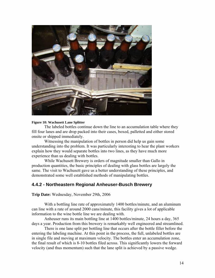
Figure 10: Wachusett Lane Splitter The labeled bottles continue down the line to an accumulation table where they

fill four lanes and are drop packed into their cases, boxed, palletted and either stored onsite or shipped immediately.

Witnessing the manipulation of bottles in person did help us gain some understanding into the problem. It was particularly interesting to hear the plant workers explain how they would separate bottles into two lines, as they have much more experience than us dealing with bottles.

While Wachusett Brewery is orders of magnitude smaller than Gallo in production quantities, the basic principles of dealing with glass bottles are largely the same. The visit to Wachusett gave us a better understanding of these principles, and demonstrated some well established methods of manipulating bottles.

4.4.2 - Northeastern Regional Anheuser-Busch Brewery

Trip Date: Wednesday, November 29th, 2006

With a bottling line rate of approximately 1400 bottles/minute, and an aluminum can line with a rate of around 2000 cans/minute, this facility gives a lot of applicable information to the wine bottle line we are dealing with.

Anheuser runs its main bottling line at 1400 bottles/minute, 24 hours a day, 365 days a year. Production from this brewery is remarkably well engineered and streamlined.

There is one lane split per bottling line that occurs after the bottle filler before the entering the labeling machine. At this point in the process, the full, unlabeled bottles are in single file and moving at maximum velocity. The bottles enter an accumulation zone, the final result of which is 8-10 bottles filed across. This significantly lowers the forward velocity (and thus momentum) such that the lane split is achieved by a passive wedge.

15

This Anheuser-Busch plant does not use any form of a high speed lane splitting mechanism.

4.5 - Other High Speed Line Split Solutions Research was conducted on high speed lane split solutions through patent searches and commercially available products.

4.5.1 - Patent Research There are currently several different patent ideas on how to conduct a high speed

lane shift of a container on a conveyor. Many of these ideas are for single container rejection, not for dedicated high speed lane shifters. The abstracts of each patent can be found in Appendix A. All patents research was gathered from www.freepatentsonline.com.

4.5.2 - OEM Products As stated before there are several products on the market that have the ability for a high speed lane shift, however, most of the products serve as rejection systems, not dedicated lane splitters. Listed below are several companies that manufacture mechanism to cause a diversion of a container from one path to another.

4.5.2.1 - Heuft Heuft offers several different solutions to the lane diversion/rejection system, most of which are patented by the founder of the company. The following list is Heuft’s current line-up of commercially available products for lane splitting.

16

4.5.2.1.1 - Heuft Delta-K

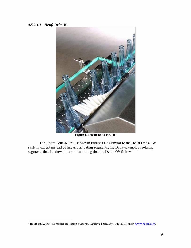
Figure 11: Heuft Delta-K Unit2

The Heuft Delta-K unit, shown in Figure 11, is similar to the Heuft Delta-FW system, except instead of linearly actuating segments, the Delta-K employs rotating segments that fan down in a similar timing that the Delta-FW follows.

2 Heuft USA, Inc. Container Rejection Systems. Retrieved January 10th, 2007, from www.heuft.com.

17

4.5.2.1.2 - Heuft Flip Rejecter

Figure 12: Heuft Flip Rejecter3

The Heuft flip rejecter shown in Figure 12 is a single arm actuator that simply pushes a single container transversely across the conveyor. It is a simple robust option for single container rejection. 4.5.2.1.3 - Heuft XY The Heuft XY is a multi-segmented linear actuation system shown in Figure 134 capable of multi-lane sorting of containers. It is ideal for sorting as it can divide containers into up to four lanes. This system is most suitable for low speed applications

4.5.2.2 - KHS KHS is a respected company in the production industry.

3 Heuft USA 4 Heuft USA

Figure 13: Heuft XY4

18

KHS does not offer any dedicated lane splitters, however, they offer a unique system that double-files a single file line of bottles. This system could potentially be used in conjunction with a passive wedge lane divider. An example photo is shown in Figure 14.

Figure 14: KHS Waveform5

Figure 15: Top view of KHS Waveform6 This system is interesting as it uses two spinning belts with complementary waveforms such that as bottles are fed through, they are laned in a staggered double file line. This system could function as a unique laning system if the double file line was then split with a passive wedge.

5 KHS. Container Conveying Solutions. Retrieved November 19, 2007 from www.kisters.com/img/pool/1111_Container%20Conveying%20Systems.pdf. 6 KHS

19

4.6 - Rapid Prototyping Rapid prototyping is the modern production method of forming solid parts from a CAD model without the use of traditional fabrication techniques. Complex geometries can be formed more quickly for less initial investment than other methods. There is no need for a mold, and typically no secondary operations are necessary. Part accuracy is generally quite good, depending on the process and materials used. The general concept behind rapid prototyping is to divide the CAD model into many cross sections, and then to build a physical part by accumulating these sections one on the other. There are numerous means of accomplishing this, using stock material in the form of sheets, powder, liquid, resin or wire. The process allows the fabrication of otherwise non-machinable geometries, as seen in Figure 167. More detailed information on rapid prototyping techniques can be found in Appendix J.

4.7 - Servo Motors Servo motors are, in basic terms, an electric motor with a brain. Servos as described by Robert Norton in Design of Machinery, are “fast-response, closed loop controlled motors capable of providing a programmed function of acceleration or velocity, providing position control, and of holding a fixed position against a load”8. The control is based on the closed loop system, which means that sensors on the servo feed back information on the motor’s position and velocity to the controller. The controllers are called drivers, which is a computer that responds to the information and adjusts the current flow to drive the motor. The drivers can be programmed to control the servo motor dynamically to adjust for changes in load and commands. The commands can be input in real time through user interface or can be imbedded in a cycle program. Servos can be configured in both AC and DC, have high torque capability and perform well in instances needing rapid acceleration and deceleration. They are capable of providing tight toleranced constant velocities, even under dynamic loading.

Servos are gaining rapid acceptance at Gallo, making complicated operations easier to automate. In the last five years, servos have found their way to several of the bottling lines and continue to be implemented.

7 Figure retrieved from http://www.cs.berkeley.edu/~sequin/SCULPTS/SnowSculpt02/maquettes.html 8 Norton, Robert L. Design of Machinery. New York: McGraw Hill, 2004, page 70.

Figure 16: Complex Geometry Realized Through Fused Deposition Modeling

20

Chapter 5.0 - Camoid Design Conception

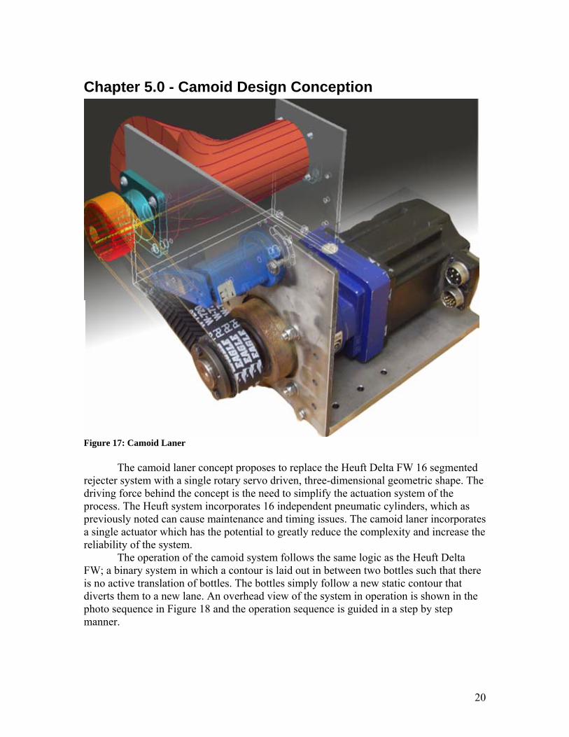
Figure 17: Camoid Laner The camoid laner concept proposes to replace the Heuft Delta FW 16 segmented rejecter system with a single rotary servo driven, three-dimensional geometric shape. The driving force behind the concept is the need to simplify the actuation system of the process. The Heuft system incorporates 16 independent pneumatic cylinders, which as previously noted can cause maintenance and timing issues. The camoid laner incorporates a single actuator which has the potential to greatly reduce the complexity and increase the reliability of the system. The operation of the camoid system follows the same logic as the Heuft Delta FW; a binary system in which a contour is laid out in between two bottles such that there is no active translation of bottles. The bottles simply follow a new static contour that diverts them to a new lane. An overhead view of the system in operation is shown in the photo sequence in Figure 18 and the operation sequence is guided in a step by step manner.

21

Figure 18: Camoid Extension

A. Bottle 1 passes by the camoid. Bottle 2 approaches. B. Both Bottle 1 and Bottle 2 are passing the camoid. C. Bottle 1 continues to Lane 1. Bottle 2 is still in contact with the Low Dwell of

the camoid. Bottle 3 enters the beginning of the camoid. D-F. The cam rotates, with Bottle 3 riding the High Dwell while Bottle 2 is riding

the Low Dwell simultaneously. G. Bottle 2 continues to Lane 1. Bottle 3 is riding the High Dwell of the camoid. H-I. Bottle 3 continues to Lane 2.

Once the contour is laid out, the camoid will remain in the diverting (on) position

until a given number of bottles passes, and then the camoid will begin to spin and the camoid will return to the off position. The camoid will remain in the off position for a given number of bottles, then repeat the process described above.

The operation is very similar to the Heuft Delta FW, but the design offers improvements that will positively affect the reliability of the system. In this chapter the camoid laner mechanism will be explained in a manner to give a basic understanding of the concept and introduce some terminology before detailed investigation into the design process ensues in the proceeding chapters.

22

5.1 - Camoid Geometry

5.1.1 - Camoid Concept The heart of the camoid laner is the camoid geometric shape. By definition a

camoid is a two degree-of-freedom, three-dimensional cam. Two degrees of freedom means that the shape can cause motion in two directions. Putting this into perspective for a bottle laner, the two degrees of freedom can be described as follows:

• First degree of freedom: The bottles traveling down-line on the conveyor, x-direction

• Second degree-of-freedom: The bottles being diverted across the conveyor, y-direction

5.1.2 - Camoid Inspiration Heuft currently has several rejecters on the market as explained in the background section (Chapter 2), and one of which sparked the idea to use a camoid for the laner design. The Heuft Delta K shown in Figure 19 is similar to the Heuft Delta FW 16 system used on the lines currently; however, instead of linearly translating segments, this system uses rotating fingers. The timing would be similar to the Heuft Delta FW; just the actuation motion would be changed.

Figure 19: Heuft Delta-K Bottle Rejecter9

As stated before, the driving force of the idea is to reduce the number of actuators. The camoid design stems from the concept of the Heuft segments and timing wrapped about a single axis, effectively controlling timing, translation and contour in a single geometry provided rotation can be controlled accurately.

9 Figure retrieved from Heuft USA

23

5.1.3 - Camoid Design

Figure 20: Camoid Laner Shape The camoid laning geometry is basically the Heuft segments physical nature and

actuation control logic wrapped about a single axis. This is easier to understand by examining the Heuft geometry and timing in detail. In the following sections, the process for generating the complex geometric shape shown in Figure 20 will be explained in basic terms providing the necessary background and terminology for understanding of the more detailed analyses in the proceeding chapters.

Figure 21 shown below is an explanation of the terminology used in this section.

24

Figure 21: Geometry Terminology

5.1.3.1 - Wrapping Segments Around an Axis It’s easiest to understand the shape if it is explained as a series of cross sections acting like cams with a common rotational axis (camshaft). Each segment of the Heuft Delta FW system can be modeled as a double dwell two-dimensional cam with the cam’s high dwell to be equal to the segment displacement and low dwell to be equal to the base circle. This is easiest to explain with the cam segment graphic shown in Figure 22.

25

Figure 22: Cam Segment Construction The cam segment construction is actually quite simple. It consists of two concentric circles, the base circle and cam rise circle. The base circle is representative of the Heuft off position, i.e. all segments not actuated. The cam rise circle is representative of the Heuft on position, its radius equal to the Heuft segment length. The cam rise circle whose chordal length is related to a high dwell angular displacement. The importance of this value will be discussed later in the report in Chapter 7. A tangent line, labeled in Figure 22, is extended from the base circle to either extreme of the cam rise circle section.

If all 16 cams are stacked along the shaft, the resultant shape long drum cam with each successive cam rise making the contour of the Heuft segments. To do this, the base circle of each cam segment remains constant, while the cam rise circle of each cam section represents the length of the corresponding Heuft segment. If we were to spin this, the contour would rise and fall; however each cam’s rise would occur simultaneously. From researching the Heuft timing in the previous chapter, we know that the segments fire in sequence between two bottles, they do not actuate simultaneously. The next step with the camoid laner geometry is to sequence the rise such that it resembles the Heuft sequence and allow each cam’s successive rise to occur between two bottles.

26

5.1.3.2 - Sequencing the Cam Rise The main goal is to cause the rise of each successive cam segment to occur between two bottles. If the bottles were not moving parallel to the axis of rotation, the cams could rise simultaneously and remain rising between the two stationary bottles. As we know, this is not the case. In order to cause the cams to rise in succession, each successive cam is out of phase to the previous cam some angle in the direction opposite to the rotation direction of the camshaft. This phase shift is shown in Figure 22. This causes each successive cam to delay its rise during rotation of the camshaft, provided the cam shaft is spinning at constant rotational velocity. Figure 23 is a representation of what the shape would look like at this point in the explanation. Notice that the cam segments rise wraps around the cam shaft axis in a helical manner. It is this helical shape that allows the cam segments to sequentially rise between two moving bottles during constant cam shaft rotation.

Figure 23: Segmented Camoid

Before the explanation goes further it is important to note that the rise profile (tangent lines connecting high and low dwells) of the cam segments is in no way involved in manipulating bottles. The bottles are only in contact with the cam segments high and low dwell surfaces. It is the succession of rising cam segments which creates the profile by which the bottles are diverted.

5.1.3.3 - Smooth Diversion Both the basic shape of the camoid and basic functionality behind the shape have

been described thus far. However, the resolution of the contour is poor with sixteen segments, especially if the segments are not blended together, as they are shown in Figure 23. This resolution is crucial as the bottles will be in contact with this section of the cam and an unblended surface could cause damage to bottles. There are two criteria that must be met in order to create a smoothly rising contour:

a) The thickness of each cam segment must approach zero b) The successive cam segments must rise according to a function that provides

satisfactory results in the output bottle motion (acceleration, velocity, etc.)

27

As the cam segment thickness approaches zero, the resolution of the contour increases, creating a smoothly blended surface that would resemble the shape shown in Figure 20.

The rise succession of the Heuft Delta FW segments does not provide the resolution needed for the contour design; therefore it is necessary to provide a function that governs the successive rises of the cam segments. Since the bottles will be being diverted by this contour, it is important to make sure that the contour will not cause any unwanted or dangerous forces on the bottle as it is being diverted. One method to mathematically ensure an effective contour is to use cam program design.

5.1.3.4 - Contour Design If we treat the bottle as a follower and the contour as a cam rise profile, we can use cam design methodology to ensure that the displacement, velocity, acceleration, jerk and force caused by the contour are all satisfactory. For a baseline of comparison, the Heuft contour was reversed engineered and then compared to several different cam programs to find the must effective contour. The cam design is explained in more detail in the following sections.

5.1.3.5 - Broad Details of Segment Phase Shifts The segment rises are controlled in a manner such that the bottles are gently diverted, it is crucial to time the segment rise sequence effectively. This sequential introduction of cam segment rises is cause by the angular offset, or phase shift, of each segment to one another. There are several things to remember when interpreting the phase shift of the cam segments:

a) The phase shift must be large enough such that the contour rises only between two bottles

b) It must be large enough to provide a point in camshaft rotation at which all segments are at high dwell, i.e. a continuous strip of contour for bottle diversion (this will be explained in the next section, Controlling the Servo).

c) It must not be too large to allow the contour to fall between two bottles.

28

There are only 360 degrees to work within for the phase shift that will allow both a cam segment rise and fall within one rotation. Notice in Figure 24 the phase shifting can be clearly seen by the curve dotted in green. Note that if there were no phase shifting, the dots would make a straight line along the camoid axis, not a curve.

Figure 24: Cam segment phase shifting

5.1.3.6 - Bottle Contact Strip An important criterion constraining the phase shifting is the necessity of a period in cam rotation at which all cam segments are in high dwell. The reasoning behind this can be explained by the nature of the concept. The system must be binary and the camoid must remain in one position while a given number of bottles are being diverted. This requires a section of the camoid to offer a continuous section of contour at a point in its rotation. An example of the strip is shown in Figure 25. Notice that there is a strip on both the low dwell and the high dwell of the camoid, representing no diversion on the low dwell and positive diversion on the high dwell of the bottle respectively.

Figure 25: Sections of Continuous Contour

29

Correctly designing the phase shifts will result in a contour strip of satisfactory width. However, it is a delicate process as different parts of the camoid geometry can be drastically altered with a small change in phase shift. These variations will be discussed in detail later in the report as there are actually several geometric variables that can be adjusted to create a satisfactory contour strip. For the purposes of this section we will not discuss these details.

This strip actually serves two purposes, one of which is offering the continuous contour. In the following section we will see how the contour strip plays a significant role in the timing of the rotational actuation.

5.2 - Actuation Design If the camoid geometric shape is the heart of the camoid laner mechanism, then the actuation system is the brain. As stated previously, the actuation of the camoid laner is accomplished by a servo motor. There are several key reasons as to why the servo motor was chosen over other actuation methods and in the following subsections of this chapter, these reasons will be introduced. Again, greater detail and analysis behind these decisions can be found in later chapters; however it is necessary to have a basic overview understanding of the actuation system and terminology before any detailed explanation could be interpreted. Topics of investigation of the actuation system in this chapter include:

• Why use a servo? • Choosing the servo • Sizing the servo • Controlling the servo

5.2.1 - Why use a Servo? As discussed earlier in the chapter, the nature of the camoid operation calls for several required actions during operation:

• The actuation of the system is rotation • During laning process, the rotational velocity of the camoid must be constant • The camoid must remain at both high and low dwell (no rotation) for a given

number of bottles to pass

There are also several task specifications that must be adhered to: • The mechanism must be able remain in either on or off position (high or low

dwell) for extended periods of time • The mechanism must accommodate for variable line speeds • The mechanism must be frequency adjustable, i.e. change the number of

bottles to pass From these constraints we can also deduce further requirements of the actuation system:

• The system must accelerate to a full rotational operating velocity between two bottles

• The system must decelerate as quickly as possible

30

• The system must be adaptable for actuation start times based on a number of inputs including o Bottle velocity o Bottle position

• The operational rotational velocity must be a function of the line speed, since the mechanism must adapt to different line speeds in real time

• The system must offer high torque outputs due to high acceleration requirements

Based on the requirements of the actuation system, it is apparent that the actuation

must be under careful control. From the discussion about servo motors in the previous chapter we can see how a servo can fulfill the requirements of this application. Recall that servo motors offer:

• Fast response time • Position control • Capability to hold a fixed position • Velocity and acceleration program control • Rapid acceleration and deceleration capability • Tight toleranced constant velocity even under dynamic loading • High torque capability

To achieve the level of control needed by a single rotational actuator, the servo is

an excellent candidate.

5.2.2 - Choosing a Servo Gallo currently is installing an increasing number of servo motors as more precise automation, higher quality and easier production operation is demanded by the company. For this reason, Gallo works closely with a well known and trusted servo automation company, Rockwell Automation. Rockwell provides all the necessary hardware and software to power and control the Allen-Bradley servo motors that Rockwell distributes. Choosing a servo brand to use in this case was dependent on the sponsor company preference.

5.2.3 - Sizing a Servo Choosing an appropriately sized servo is an important task and care must be taken in doing so. In this case of high accelerations, a servo motor with sufficient torque is necessary. Choosing a servo with insufficient torque will result in the mechanism not accelerating in time, potentially causing damaged bottles. Over-sizing the servo is expensive and unnecessary. A large servo may also not have the acceleration necessary because of high motor inertia. In order to aid in the process of sizing a servo, Rockwell Automation offers software that will provide a range of servos that would be applicable based on a number of user defined constraints and timing criteria. This will be explained in greater detail in later chapters.

31

5.2.4 - Controlling the Servo The servo is controlled through a series of components that compose a closed loop communication system. Information regarding all aspects of the motion is relayed in real-time to adjust the output to accomplish the exact task demanded by the user. Designing a control program for a servo requires attention to detail. After choosing the correct servo and driver components, the general constraints on the motion of the servo are:

• Position • Operating Velocity • Acceleration • Start Time • Dwell Time

5.2.4.1 - Position In the case of the camoid laner, the exact position of the servo is essential information to provide the control logic as it is crucial in the successful operation of the system. To accomplish this, the servo motor is equipped with a shaft encoder that feeds back its position data to the control system.

5.2.4.2 - Operating Rotational Velocity The contour must be laid out between two bottles, thus the rate at which the

contour rises is equal to the bottle velocity. This velocity is essential to successful operation and must match the bottle velocity at all times, thus is denoted as the operating velocity. The operating rotational velocity is calculated based on the linear velocity of the bottles on the line.

5.2.4.3 - Acceleration The servo needs time and distance to accelerate and decelerate the camoid up to/down from the operating velocity. In order to accomplish this, both the geometry of the camoid and the timing of the actuation must be adjusted. Recall that in order for successful diversion of the bottles, the camoid geometry must incorporate a continuous strip of contour running its entire length. Not only does this strip act to provide a continuous contour, but also provides the buffer distance for servo acceleration and deceleration.

5.2.4.4 - Actuation Start and Dwell Times The start of the actuation and the camoid dwell time are both matters that require sensing bottle positions. The actuation must initiate between two bottles. The camoid must dwell for an amount of time that is dependent on the number of bottles that it diverts. In order to accomplish these tasks, the servo controller must be aware of the bottle positions and how many bottles have passed the laner. To do so, a photoeye is placed on the line that reads when a bottle goes past it. Alone the photoeye is capable of counting bottles as they pass. When coupled with the shaft encoder, the two instruments are capable of sensing a bottle’s position as it moves down the line. With this information

32

input to the servo controller, the actuation initiation and the dwell timing are able to be controlled.

5.2.5 - Actuation Design Conclusions The properties of a servo make it an ideal candidate for the motion application of the camoid laner. With the servo, all aspects of the motion can be controlled in detail and adjusted in real-time to accommodate a wide range of scenarios that could be experienced out on the line.

5.3 - Design concept summary Coupling geometric design with proper motion control, the camoid laner is able to accomplish with one actuator what the Heuft Delta FW does with sixteen actuators. Not only is the number of actuators fractioned, but the reliability of the actuation method is increased as well. This chapter was intended to give an overview of the concept behind the design and to introduce some of the terminology that can be expected in the following sections. In the next chapters the camoid design will be explained in detail with mathematical analysis to support the decisions made in the design. Each section will include a brief introduction to the specific aspect of design to be explained; however, if there is any confusion before reading the analysis, this chapter should be referenced.

33

Chapter 6.0 - Methodology This chapter outlines the steps that were taken throughout the design process and present the process in a logical order that could be replicated. The actual methodology involved simultaneity and iteration.

6.1 - Assumptions A number of assumptions were made throughout the design phase of this project. Such assumptions are necessary to prioritize different elements in both the problem definition and the derived solution. Some of the most relevant assumptions are briefly discussed here, along with any verification that the assumptions were valid.

6.1.1 - Line 2 Properties The process of splitting bottles is heavily dependent upon an accurate kinematic model of a stream of bottles, including their relative positions, velocities, and accelerations. The relation between bottle and conveyor is also of great importance. Considering this, an average set of conditions was taken as the design baseline, with all analyses and decisions made in reference to these conditions. The design should allow for a safe range of conditions around the average. Line 2 runs at a rate of 400 bottles per minute when operating correctly. This equates to a conveyor roughly 1 meter per second. Based on accounts from Gallo employees and video footage, it was determined that wine bottles on Line 2 were in static friction with the conveyor at the point of the lane split. An assumed minimum bottle spacing (the distance between two adjacent bottles) of one bottle diameter was agreed upon, again through the advice of Gallo engineers. These conditions describe bottles with no relative velocity, neither to each other nor to the conveyor, and with velocity equal to the line speed relative to the stationary splitter.

6.1.2 - Heuft Laner The direction of the redesign was largely defined upon making one assumption in particular; the laning system currently used by Gallo is successful at its function of diverting bottles, but fails to achieve the desired lifetime. Prior to making this assumption, the design team had looked at alternative methods of achieving a laning diversion. With this assumption, however, the focus shifted to finding alternative means of driving the existing system to improve lifetime. The shift in focus was significant. It made analyses on tipping or breaking bottles less important; if the Heuft Laner did not damage bottles with its current means of actuation (pneumatic cylinders), it follows that the bottles would remain undamaged if the actuation was replaced, but mimicked closely enough.

34

6.2 - Data Collection and Analysis

6.2.1 - Heuft Analysis The design requirements of this project are to improve upon the existing design for high speed lane splitting. In order for this to be accomplished, the existing system must be analyzed and understood. The first step taken was to understand key aspects of the operation of the Heuft laning system. The method by which the mechanism functions is explained in the background chapter of this report.

The next step in understanding the Heuft laning system was to analyze the contour by which the bottles are diverted. An understanding of the function of the contour is needed as a baseline of comparison for other contours.

The Heuft contour was measured and a best fit polynomial equation was fit to the points measured. The contour can be understood mathematically allowing kinematic and dynamic analyses can be conducted.

Heuft Contour and Approximate Equation

y = 0.0011x3 + 0.0166x2 + 0.0362x - 0.0007R2 = 0.9999

-0.500

0.000

0.500

1.000

1.500

2.000

2.500

3.000

0 1 2 3 4 5 6 7 8 9 10

Downline Travel (in)

Cro

sslin

e St

roke

(in)

Heuft ContourApprox

Figure 26: Heuft Contour and Equation

6.2.2 - Contour Design and Analysis The most important aspect of the design is that no bottles are tipped or damaged during the laning process. In order to improve on the existing system, cam program design is used to develop several contours with controlled acceleration profiles. Based on standard cam design methodology10, we chose three different cam programs to use as a base for optimization of the existing system. The three cam programs of interest are as follows:

• Simple Harmonic Displacement • Modified Trapezoid Acceleration • 4-5-6-7 Polynomial Function Displacement Each of the programs is designed following some basic criteria that require

specific aspects to be constrained.

10 Norton, Robert L. Design of Machinery. New York: McGraw Hill, 2004.

35

6.2.2.1 - Simple Harmonic Displacement Constraints Constraints are set on the final value of displacement.

6.2.2.2 - Modified Trapezoidal Acceleration Constraints Assumptions are made of the maximum allowable acceleration.

6.2.2.3 - Polynomial 4-5-6-7 Function Displacement Constraints By adjusting the values of the 8 constants, constraints can be set on the initial and final position, velocity, acceleration and jerk (boundary conditions). Polynomial cam contours offer accurate control of the dynamic conditions at the selected positions, however the displacement function is governed by the boundary conditions and is often difficult to control maximum values.

After specific contours are designed and plotted, they are compared against the existing system, and analysis is conducted on each contour.

6.2.2.4 - Kinematic Analysis Kinematic analysis includes comparison and discussion on each of the cam displacement, velocity, acceleration and jerk profiles. The three proposed profiles are directly compared with the current Heuft system and are also compared with each other. Topics of investigation include:

• Difference compared to Heuft • Abnormal peaks • Maximum values • Minimum values

6.2.2.5 - Force Analysis Force analysis was conducted with the same criteria listed above in kinematic analysis except analyzes the force and moment induced by the contour on the moving bottle. In addition, the force and moment were compared to the friction force between the bottle and conveyor making sure that the contour will induce enough force to overcome static friction fast enough to minimize tipping potential.

6.2.3 - Choosing Contour The most suitable contour is chosen based on several important criteria: • Acceptable Final Velocity • Minimizing Maximum Acceleration • Minimizing Jerk • Maximum Force • Maximum Induced Moment on Bottle

The last two criteria are most important as both are involved directly with

damaging and tipping bottles. Taking each of these criteria into consideration, a contour is chosen that best suits high speed bottle laning.

36

6.3 - Camoid Geometry Design The design of the camoid geometry is an iterative process. There are several elements of the camoid that are manipulated to generate the complex geometry. The elements are interdependent; changing one element affects the others, which in turn affects the entire geometry of the camoid. The elements of the geometry that are manipulated are:

• Profile Rise Contour • Cam Phase Angles • High Dwell Angle Displacement • Low Dwell Angle Displacement • Buffer Angle • Base Circle Radius • Overall Length of Laner

This detailed design process can be found in detail in Chapter 7 of this report.

6.3.1 - Manufacture It was agreed early that the material of the camoid will be some sort of plastic for its characteristics in:

• Wear resistance • Oxidation resistance • High strength to weight ratio • Low weight • Forgiveness for bottles during impact (relative to metal) • Manufacturing flexibility • Low cost

The geometry of the camoid is complex and could prove to be difficult to

manufacture for conventional methods of machining. Furthermore, the geometry must be relatively accurate as there are tight tolerances of certain elements. There are few options available for manufacturing complex geometries:

• CNC Machining • Rapid Prototyping • Injection Molding

Each method offers advantages and disadvantages shown in Table 1.

37

CNC Rapid Prototyping Injection Molding Adv. Disadv. Adv. Disadv. Adv. Disadv.

Inexpensive (relative to

other methods)

Limits of geometric

complexity due to tooling and nature

of process

Complex Geometries Expensive

Inexpensive for large quantity

orders

Expensive for single part order

Large Material Variety Fast turnover Material

Limitations Large Material

Variety

Limits of geometric

complexity (mold still must be machined)

Many companies Availability

Issues

Table 1: Manufacturing Method Comparison

Due to the complex geometry of the design, the most logical choice for manufacturing was rapid prototyping. However, there are several different methods for rapid prototyping that offer a set of advantages and disadvantages. The rapid prototyping comparison can be seen in Table 2.

Stereolithography (SLA)

Fused Deposition

Modeling (FDM) Selective Laser Sintering (SLS)

Electron Beam Melting (EBM)

Adv. Disadv. Adv. Disadv. Adv. Disadv. Adv. Disadv.

Most commonly

used

Slower than other RP methods

Produces robust parts

Less accuracy than SLA

Material Variety

Less accuracy than SLA

Material variety

(same as SLS)

Immature Technology

Accurate Parts not as

robust as other

Material variety

Secondary curing

needed

Secondary curing

unneeded

Porous parts

Non porous, homogenou

s, robust parts

(titanium)

Expensive

Secondary

curing needed

Faster and more

efficient than SLS

Support structure may be needed during

production process

Support structure may be needed during

production process

Accurate

Table 2: Rapid Prototyping Method Comparison After researching the methods of the rapid prototyping the search was narrowed down. For the purpose of the camoid laner, SLS is not appropriate because the part cannot be porous due to the moist environment and the part must be smooth. EBM is too expensive and a titanium part is unnecessary. This leaves SLA and FDM to choose from. Stereolithography was the method of choice for several reasons:

• Adequate material strength

38

• Accuracy is needed on several sections of the camoid, especially a keyway • Best price offer • Best turnover time See Appendix B for a full list of prices and companies that were considered.

6.4 - Actuation Design The timing and geometry criteria must be strictly adhered to for the successful

operation of this laner. Once this information is known, analysis can be conducted on the rotational velocity, accelerations, and torques required to achieve successful timing.

6.4.1 - Sizing a Servo Accurate sizing of the servo is important because of the precision needed in this

application. An undersized servo will not create the accelerations needed to reach operating velocity in the buffer angle given. An oversized servo is more difficult to tune and is more expensive to purchase and operate.

Allen-Bradley motors are Gallo’s trusted motor company and currently offer free software11 to aid in the sizing of A-B servo motors to fit specific applications. The Rockwell Motion Analyzer software is used to accurately size the servo to this camoid application.

The software accurately sizes a servo based on several input values including: • Voltage Supply type and nominal value • Velocity-Time cycle profile (timing diagram) • Mechanism data

o Inertia Values o Starting angle

• Transmission data o Type (belt, spur, etc.) o Ratio o Efficiency o Friction

Once these values are input, the software searches an internal database of the A-B servo product line and produces a range of motors that fit the criteria entered. Motor data accompanies the motor models including, but not limited to:

• Peak velocity • Peak and RMS torque • Current Draw • Gearbox ratio • Relative Cost (to motors in search results) • Relative Performance (to motors in search results)

11 Rockwell Automation. Motion Analyzer Software. Retrieved February 11, 2007 from

www.ab.com/motion/software/motion_analyzer.html

39

The motor list can be arranged according to the user’s desire. The software also runs graphical torque analysis comparing the torque-speed diagram to the user required torque.

The software offers a detailed, motor model specific comparison allowing accuracy and confidence when attempting to size the servo to the application.

6.5.2 - Controlling the Servo Along with camoid geometry, the control logic of the servo is the most important part of successful operation of the camoid laner mechanism. There are several pieces of hardware and software required to get from the control logic concept to the output motion of the servo. These elements are:

1. Control Logic Software 2. CPU Interface Module 3. Servo Driver 4. Servo

Together these elements make a closed loop information chain to create and adjust the servo motion exactly to specifications and real-time data feeds. These elements will be explained in greater detail in Chapter 7

It should be noted that the control logic is designed in specific software offered by Rockwell Automation. The logistics of the software and the programming protocol12 will not be explained in this report as Gallo employs specifically trained engineers for servo controls. However, the servo actuation sequence will be explained and how it is directly related to the camoid geometry.

The specifications for the servo control program was written by the camoid design engineers as it is important to follow the correct criteria that Gallo demands for servo motion control. There are several safety issues concerning servo operation and must be included. For this reason, the actual servo control program writing was outsourced to David Booth of Gallo’s Controls department.

6.5.2.1 - Assumptions • The camoid must begin spinning such that the contour rises and remains rising

between two bottles. • The camoid must be accelerated to operating rotational speed as fast as

possible. • Operating speed is directly proportional to the line speed and is such that the

camoid must complete its rotation cycle in the time that one bottle travels the camoid length.

• The cam must decelerate as fast as possible.

6.5.2.2 - Timing 1. From rest (0°) position spin to high dwell at operating speed 2. Remain at high dwell for a bottle count (10 bottles)

12 Information regarding this program logic can be found at www.rockwellautomation.com/rockwellsoftware/design

40

3. Spin from high dwell to position 360° at operating speed 4. Remain at low dwell for a bottle count (10 bottles)

There are several aspects to keep in mind during this timing sequence:

a) The servo needs time and distance (angular distance) to accelerate the camoid up to operating velocity

b) The servo needs time and distance to decelerate the camoid from operating velocity

c) The operating velocity is directly proportional to the line speed (which may change at any time)

d) The amount of time the camoid remains in dwell is dependent on a number of bottles (which may be non-uniformly spaced)

Each of these aspects are worthy for investigation in this section to provide

baseline understanding of the program details explained in the following chapters.

6.5.2.3 - Operating Velocity As stated before, the successful operation of the camoid laner relies on the camoid being rotated at a constant velocity. The velocity at which it rotates is directly related to the line speed, as the contour must rise in between two bottles on the line. However, because the bottling line is subject to frequent shut downs and decreases in speed, the operating velocity of the camoid laner must be able to accommodate such instances. In order to accomplish this task, the servo controller must always be ‘aware’ of the line speed. To do so, a shaft encoder attached to the conveyor line feeds line speed information to the servo controller. The operating rotational velocity of the camoid is directly related to the line speed by a mathematical function. Once input into the controller, the servo output velocity can be adjusted in real-time to accommodate the dynamic conditions of the bottling line.

6.5.2.4 - Servo Acceleration and Deceleration The servo needs time and distance to accelerate and decelerate the camoid up to/down from the operating velocity. In order to accomplish this, both the geometry of the camoid and the timing of the actuation must be adjusted. Allowing a buffer distance for the servo to accelerate and decelerate is a matter that concerns the camoid geometry. Recall that in order for successful diversion of the bottles, the camoid geometry must incorporate a continuous strip of contour running its entire length. Not only does this strip act to provide a continuous contour, but also provides the buffer distance for servo acceleration and deceleration. The strip acts as a buffer because of the fact that the camoid neither rises or falls, i.e. there is no bottle diversion. This means that the camoid can rotate a certain angle amount, the buffer angle for explicative purposes, without a bottle being manipulated. This becomes necessary as the servo can use this buffer angle to accelerate and decelerate after it has completed its operating cycle.

Adjusting the timing to allow for servo acceleration and deceleration is a matter of starting the actuation somewhere within the buffer angle. The buffer angle will allow

41

the servo to accelerate up to the necessary operating velocity without any bottle manipulation.

6.5.2.5 - Torque Based on the acceleration necessary and the geometry of the cam, the necessary torque to achieve the desire effects is calculated. The cam mass moment of inertia must be known for this calculation and is obtained using 3D modeling software due to the complex camoid geometry.

6.5.2.6 - Actuation Start and Dwell Times The start of the actuation and the camoid dwell time are both matters that require reading bottle positions. The actuation must initiate between two bottles. The camoid must dwell for an amount of time that is dependent on the number of bottles that it diverts. In order to accomplish these tasks, the servo controller must be aware of the bottle positions and how many bottles have passed. To do so, a photoeye is placed on the line that reads when a bottle goes past it. Alone the photoeye is capable of counting bottles as they pass. When coupled with the shaft encoder, the two instruments are capable of knowing a bottle’s position as it moves down the line. With this information input to the servo controller, the actuation information and dwell timing are able to be controlled.

6.5.3 - Stress Analysis An important consideration in the camoid analysis is stress induced from the

torque. Since the torque must be transmitted to the camoid, the method used will be a key and keyway. Several different stress analyses are conducted:

• Shaft Shear Stress • Torsional Deflection • Keyway Stress Concentration • Safety Factors with different materials

6.5.4 - Fatigue Stress Analysis The nature of the splitting operation is such that the camoid is subject to cyclic application of torque to accelerate and decelerate to and from operating velocity. Thus, it is important to conduct fatigue stress analysis. The fatigue strength of the shaft is calculated to ensure adequate lifetime.

6.6 - Part Gathering An important part in this design process was finding the correct parts needed to build the prototype. A full bill of materials can be found in appendix C

6.7 - Chassis Design The last step in the process is to design the frame, or chassis, that will house the system. There are several points of interest of the design that warrant discussion:

• Material

42

• General layout of components • Implementation on bottling line • Manufacturability

6.7.1 - Material There are several criteria that the material must meet:

• It must not oxidize • It must not be toxic • It must be structurally sound The must common structural materials used in Gallo’s bottling lines are steel,

stainless steel and aluminum. Each material offers advantages and disadvantages which are shown in Table 3.

Steel Stainless Steel Aluminum Adv. Disadv. Adv. Disadv. Adv. Disadv.

Inexpensive Oxidizes Resists Oxidation Expensive Resists

Oxidation Expensive

Strong

Requires Surface Finishing

(paint)

Widely accepted for food handling

Availability Issues

Less Strength and Toughness

(relative to steel)

Tough Strong

High Availability Tough

Table 3: Material Comparison

An important issue to keep in mind is that the chassis will be in a section of the bottling line in which there are open containers of product. The environment is wet from spilt product, line lubrication, and cleaning activities. It should be noted that Gallo requires all steel parts to be painted with a specific grade paint to resist oxidation of the steel and chipping.

6.7.2 - Component Layout The layout of the components is important as it determines the overall size of the mechanism as well as the layout of the transmission for the camoid. The layout for the mechanism can be seen in Figure 27.

43

Figure 27: Component Layout

There are several ways to drive the camoid; one idea was to directly couple the camoid shaft with the servo shaft. However, the chosen layout is advantageous for several reasons:

• Minimizes overall length of the system • Fits within the footprint of the Heuft Delta W 16 system • Keeps motor away from conveyor line • Allows easy motor access for maintenance/replacement

6.7.3 - Implementation on Line The chassis design must be designed such that the implementation on the bottling line is accomplished easily. The nature of the design is such that it is a direct replacement of the Heuft system. It will utilize the same method for attachment that the Heuft currently uses. Figure 28 shows the current method by which the Heuft system is attached to the line. Notice that the entire system is independent from the line. It is simply bolted to the side of the conveyor on the front edge and supported in the back by a single leg. The camoid laner chassis will be designed to be implemented on the line in a similar fashion to the Heuft system. This implementation method is advantageous as it allows for easy initial installment and easy replacement if needed.

44

Figure 28: Heuft Attachment to Line

6.7.4 - Manufacturability The chassis is a simple, easily manufactured design consisting of several plates fastened together with bolts and supported by several brackets ( Figure 27). The most difficult part of the manufacturing process will be drilling the bearing mount holes to fit the tolerances needed for the shaft to spin freely. Fully toleranced technical drawings were provided to the machining company.

6.8 - Drive System There are many different power transmission systems commercially available. In

order to narrow down the options, the design of the drive system must be constrained. The power transmission from the servo to the camoid needs to be a robust system that meets several criteria:

• positive transmission • low backlash • low friction • low inertia • smooth/quiet operation The easiest method for positive transmission with low backlash is to incorporate

teeth into the transmission. Spur gears and chain drives were the first options explored, however either option could present problems and not meet the desired criteria.

The cam shaft and servo shaft are relatively far apart as the distance between must clear the high dwell of the camoid and the servo body. This distance would require two relatively large diameter spur gears, which would increase the inertia. Furthermore, the

45

spur gears could cause unwanted noise. A chain and sprocket drive could be used; however this could also cause unwanted noise and high inertias.

Gallo employs a large number of transmissions on the bottling lines to drive power from a motor to a conveyor. On newer lines, a specific type of toothed belt and sprocket system is used, similar to an automobile engine timing belt. After consulting Mr. Loel Peters, the benefits of this transmission became apparent; ability to handle high torques, offer low backlash and availability in Gallo’s storeroom.

The Goodyear Eagle Pd Belt and sprockets incorporate a double herringbone tooth pattern which prevents both tangential and lateral belt slip (off the side of the sprocket). The system met all criteria set forth, provided immediate availability and was an economic solution. Furthermore, Gallo trusts the system enough to employ it elsewhere in the plant.

6.9 - Mechanism Assembly The mechanism is fastened with hardware obtained from Gallo’s storeroom. Once

built, the mechanism was subject to an initial motion test at a simulated 600 bottles per minute for one hour to assure the mechanism was functional. During the test, observations were noted of any abnormalities such as:

• Immediate Wear • Noise • Heat due to friction • Loose parts

Tests proved to be successful and no readjustment was necessary.

6.10 - Implementation Implementation on the line is under the supervision of Jason Elliot of Aubry

Construction Company. The line used to test the laner is a test loop previously installed by Gallo employees. The loop is open to allow for testing of new equipment.

46

Figure 29: Test Loop The test loop rails were adjusted to our design specifications. The test loop

includes all necessary hardware including photo eye and shaft encoder. No housing for the electronics was constructed; therefore all electronics must be

portable and temporary as Gallo safety rules do not allow uncontained electronics, especially those operating on 480V. The servo driving system was attached to a flat plate and carted to the test loop. It was removed immediately after the testing and never left unsupervised.

David Booth supervised the setup of the electronic systems assuring all safety guidelines are followed.

6.11 - Testing Testing was conducted following a detailed test protocol found in Chapter 9.

47

Chapter 7.0 - Camoid Laner Detailed Design The detailed process of the laner design is discussed in this chapter. All final values are either given or referred to in the appropriate appendix.

7.1 - Camoid Geometry Design The camoid laner is based on the wrapping the Heuft Delta FW segment lengths and actuating time around a rotating axis. If each segment of the Heuft was represented by a cam, the segment’s linear translation would be the cam’s rise which would occur by rotating the cam. The series of the cams are attached to a common shaft with progressive rises that follow a contour similar to the Heuft segments. If the phase of each successive cam is shifted it is possible to cause the similar effect of laying the contour in front of the bottle that the Heuft accomplishes by sequentially firing the segments in front of the bottle. Finally, if the thickness of the cams approaches zero, the contour will be a smoothly blended surface.

In order to accomplish this task there are several elements of the geometry that must be designed simultaneously to offer the correct output motion, provided the actuator can be precisely controlled for angular displacement and angular velocity. In the following section the design of the geometry will be explained in detail.

Note that the design process was conducted in PTC ProEngineer Wildfire 2.0.

7.1.1 - Iterative Design Arguably the must crucial aspect to the successful operation of high speed laning is the timing at which the diversion occurs; timing tolerances can be as tight as several milliseconds. In the case of the Heuft laner, the independent linear pneumatic actuators are fired in sequence governed by the line speed. In the case of the camoid, the timing is based not only on the line speed, but also the rotational actuation and geometry. Since the timing is directly related to the geometry, careful analysis is conducted to assure that the cam behaves properly. This design process is iterative and occurs simultaneously with the rotational timing design (explained in the next section). The elements of the geometry that are manipulated for the design process are:

• Diverting Contour • Cam Phase Angles • High Dwell Angle Displacement • Low Dwell Angle Displacement • Buffer Angle • Base Circle Radius • Overall Length of Laner These elements are represented below by Figure 30, but will also be individually

represented in the following sections.

48

Figure 30: Geometric Elements

Each of these elements is manipulated and affects different aspects of the timing and bottle diversion.

49

7.1.1.1 - Diverting Contour The diverting contour is defined by the successive rises of each cam segment. This is the contour by which the bottles are guided. Each cam segment’s rise is governed by the cam programs explained in the previous section.

7.1.1.2 - Cam Phase Angles The cam phase angle is the angle that each cam is offset relative to the previous cam. This controls the rate at which the contour is laid out in addition to rotational velocity. This also affects the value of rotational speed. If the phase angles are larger, the contour will take longer to be laid out, thus requiring a faster rotational velocity.

7.1.1.3 - High Dwell Angular Displacement The high dwell angular displacement is the angle of each segment over which the high dwell spans. A crucial design criterion for the camoid is that when the camoid is fully extended, every segment of the camoid must be in high dwell. Recall from Chapter 3 that this is the contour strip. If the phase angles are larger, and high dwell angular displacement is kept the same, the strip gets thinner until it no longer exists, creating discontinuity in the contour. The high dwell angular displacement is manipulated such that the strip is kept wide enough to properly guide a bottle during camoid dwell.

Figure 32: Phase Shift Angle

Figure 33: High Dwell Angular Displacement

Figure 31: Diverting Contour

50

7.1.1.4 - Low Dwell Angular Displacement The low dwell angular displacement is similar to the high dwell, except with the low dwell of the segments. When the camoid is fully retracted, the cam segments must be in low dwell. This creates a strip of low dwell flat contour parallel to the camoid’s axis of rotation. This value is not manipulated but rather serves as a limit to the value of the high dwell angular displacement.

As high dwell angular displacement increases, low dwell angular displacement decreases. Care is taken to assure that the high dwell angle is small enough to allow adequate low dwell angular displacement.

7.1.1.5 - Buffer Angle The buffer angle is directly related to the thickness of the contour strip, it is the angle of rotation over which the strip occupies. Because there are two contour strips, there are two buffer angles. The buffer angle at the high dwell is directly a function of the cam phase angles and the high dwell angular displacement. The buffer angle at the low dwell is a function of cam phase angles, high dwell angular displacement and high dwell buffer angle. This is because the low dwell angular displacement is dependent on the high dwell angular displacement.

Care is taken to assure the buffer angle is adequate both for high and low dwell. If the buffer angle is too small, the acceleration needed will be high and require a significant amount of torque, increasing motor size and thus expense.

7.1.1.6 - Base Circle Radius The base circle radius affects the width of the low dwell strip. If the base circle is too small, the tangent line of the highest cam segment approaches the tangent line of the lowest dwell segment, effectively eliminating the low dwell. If the base circle is too large, the cam will be too large to fit on the bottling line. Furthermore, if the base circle is too large, the contact point (strip)

Figure 34: Low Dwell Angular Displacement

Figure 35: Buffer Angle

Figure 36: Base Circle

51

will be too high on the bottle inducing a potentially high tipping force. Lastly, if the base circle is too large, the part will be excessively massive and require higher torques to accelerate.

7.1.1.7 - Length of Camoid The length of the camoid affects the acceleration and thus force caused by the contour. If the camoid is too short, the working contour will rise abruptly, potentially causing high accelerations and forces. If the camoid is too long, the operating rotational velocity must increase to successfully lay the contour between two streaming bottles. This increase causes rotational accelerations to increase, thus increasing the required torque. With increased torque, motor size and expense increase as well as stress and fatigue on the system.

Figure 37: Camoid Length

52

7.1.2 - Geometry Final Values The final values of the geometric elements are shown in Table 4. It should be noted that the geometry of the camoid is a smooth blended surface; however it is broken into 11 cross sections for purposes of discussion and computer modeling.

Section Number

Contour Rise (in.)

Phase Shift (deg)

High Dwell Angle (deg)

High Dwell Buffer Angle (deg)

Low Dwell Buffer Angle (deg)

Base Circle

Radius (in.)

Camoid Length

(in.)

1 0.001 0 145 7.5 32.8 1.75 9.5 2 0.006856 12 140 3 0.052 12 135 4 0.159 12 130 5 0.333 12 130 6 0.574 14 130 7 0.883 14 130 8 1.259 14 130 9 1.703 15 130

10 2.21 17.5 125 11 2.758 17.5 120

Table 4: Camoid Geometry Final Values

7.1.3 - Geometry Construction Because of the complexity of the geometry, it is not feasible to machine the part using conventional cutting techniques such as CNC milling or lathe machines. The part is constructed using a Stereo Lithography (SLA) rapid prototyping machine. After research it was apparent that the process offered satisfactory tolerances and material strength. Outsourcing the part for manufacture is a matter of emailing the correct format of the model to the company.

7.2 - Camoid Prototype Figure 38 is a picture of the comparison of the CAD model and the actual rapid prototyped part.

53

Figure 38: Model vs. Rapid prototype

7.3 - Actuation Design The servo system must provide accurate and precise actuation of the camoid through millions of cycles. Attention to detail is important in the design of the servo system. This detail is explained in this section.

7.3.1 - Servo Sizing The servo is sized using Motion Analyzer software from Rockwell Automation. For detailed tables conveying the values used for the motor sizing for this application see Appendix D.

7.3.2 - Servo System The servo system is set up to allow for completely automated control of the

actuation of the camoid based on line speed and bottle spacing. The system can adjust for varying line speeds that are experienced during line start up and shut down. It can remain in one position for extended periods of time. In order to provide the automated control, there are several important components of the servo control system that warrant discussion.

• Servo Motor • Driver • CPU Motion Control Module • Control Program Logic

54

The basic setup for the servo control system is shown in Figure 39. The system is adaptable allowing data inputs from a variety of different tools and also can be controlled remotely via Ethernet. Furthermore, the system can be configured to control multiple axes (servos) with a variety of different program profiles. The following explanation outlines one particular setup. Note that this system meets Gallo’s standards and operates on 480V 3 Phase AC electrical.

Figure 39: Servo Control Schematic

The following is a step-by-step explanation of the schematic shown in Figure 39. Each of the numbers indicates the part of the control information transfer shown in the figure. Note that there is a continuous loop of information and communication does not necessarily always occur in this sequence explained.

55

1. Control program software uploads control information to a CPU control module.

In this case the program is made with Logix 5000 software. The module simultaneously feeds back information to the computer.

2. In addition to program logic from the software, information from sensors can be input into the control module. In this case, a photoeye and shaft encoder will be used to transmit bottle position and velocity to the module. It should be noted that the control program must have the proper protocol for reading and interpreting the data from these sensors. With this input data, the program can make adjustments that answer to real-time dynamic variations in servo loading and/or timing demands.

3. The CPU control interface interprets the information of the Logix 5000 software and outputs a signal to the driver. The driver simultaneously feeds back information to the module regarding servo statistics.

4. The driver interprets the information from the CPU module and adjusts the output current to the servo motor. The servo’s internal encoder feeds back information to the driver regarding position and velocity.

7.3.2.1 - Servo Motor The servo motor was obtained from Gallo’s spare parts shelves along with the

necessary power and feedback cables. The servo motor from Gallo falls in the range of applicable motors from the Motion Analyzer software. The motor included an attached gearbox. Table 5 below is a basic overview of the motor and gearbox specifications. For more detailed specifications see Appendix E.

Figure 40: Servo Motor

56

Manufacturer Allen-Bradley Model MPL – B4520 – MJ22AA Max Speed 5000 rpm Continuous Stall Torque 6.1 N-m / 54 in.-lbs. Power 2.5 kW Gearbox Manufacturer Alpha Gearbox Ratio 10:1 Table 5: Servo Motor and Gearbox Overview Specs The servo motor includes an input and feedback cable connection. The power to the servo is delivered by the driver. Inside the servo is an encoder that reads and outputs the position of the servo through the feedback cable. The feedback is read by the driver and the power is adjusted to deliver the necessary power to follow user input controls.

7.3.2.2 - Driver The driver was obtained from Gallo’s control department from a decommissioned servo driven project. The purpose of the driver is to interpret the control logic from the computer and provide the correct electrical current to move the servo motor in the exact manner specified by the computer control logic. The input signal can be either analog or digital depending on the level of control demanded by the user. Analog is adequate for systems with a few axes (less than 6). However, for more complicated systems, digital interfacing is often used to reduce the number of connecting wires needed. Digital systems, however, are significantly more expensive. Manufacturer Rockwell Automation Model 2098-DSD-HV150 Operating Voltage 480V AC 3 Phase Peak Current (amps) 68 Continuous Current (amps) 34 Continuous Power (kW) 15 Table 6: Driver Overview Specs

7.3.2.3 - CPU Control Module The CPU interface module is the component that interprets the control logic from the computer software and outputs a readable signal to the driver. The input connection is obtained via Ethernet cable. This connection is extremely versatile enabling remote control changes over the internet. This is beneficial as it becomes possible for the control engineer to manipulate servo controls from any location that enables internet access. The modules used for this system were also obtained from Gallo’s storehouse.

7.3.2.4 - Control Program Logic The human interface of the servo control is the Logix 5000 software, which can be run on any PC with an Ethernet port (for data transfer). This software allows for the ultimate control of the servo motor. Details such as timing, position, velocity, acceleration, acceleration profiles and torque can all be controlled with fine precision. In

57

addition to servo controls, any number of safety and system check protocols can be input into the system. For example, the servo can be told to reset itself to zero after a given number of cycles to maintain system accuracy.

7.3.3 - Control Logic Concept As stated before, the logistics behind creating the control program will not be discussed in this report; however, a motion control outline is described below. There is a detailed set of constraints and assumptions and a timing diagram.

7.3.3.1 - Assumptions 1. The actuation for contour rise must begin between bottles and be at full

operational velocity a. The actuator is given a buffer angle, on the cam segments low dwell, in

which acceleration can occur. 2. The contour rise must occur at a rate such that it remains between bottles. 3. The actuation must stop and hold within the angle of the aforementioned high

contour strip. 4. The actuator must be held at this position for a data input number of bottles. 5. The actuation for contour fall must begin between bottles and be at full

operational velocity. a. The actuator is given a buffer angle, on the aforementioned high dwell

strip. 6. The contour fall must occur at a rate such that it remains between bottles. 7. The actuation must stop and hold within the aforementioned low dwell contour

strip.

These timing criteria are the baselines that must be followed for the successful operation of the camoid laner.

7.3.4 - Drive Train Specs • Final drive ratio 10:1

7.3.5 - Timing 1. From rest (0°) position spin 164° at operating speed 2. Remain at high dwell for a bottle count (10 bottles) 3. Spin from 164° to position 360° at operating speed 4. Remain at low dwell for a bottle count (10 bottles)

58

Figure 41: Timing Diagram Example

Because the timing of the motor is constantly adjusted to match the line speed, this timing diagram represents an example of the timing at a particular line speed. There are several important characteristics of the timing diagram that should be noted.

1. The x axis is time in seconds, the y axis is the angular position 2. This diagram represents a full cycle of the camoid laner. A full cycle

includes: a. Low camoid dwell, no bottles diverted b. Camoid spins such that the contour rises c. High camoid dwell, all bottles diverted d. Camoid spins such that contour falls

3. The horizontal sections of the curve represent the camoid rotation in a dwell period.

59

4. The sloped line represents the camoid during it spin a. The constant sloped section represents operating velocity b. Notice the acceleration13 up to operating velocity which occurs

between the horizontal and sloped linear segments.

The actual dwell and spin times are functions of the line speed and change according to the inputs from the shaft encoder and photoeye.

13 In the actual timing diagram, the angle over which this acceleration occurs will be the same magnitude of the buffer angle. This timing diagram is a basic theoretical representation.

60

7.4 - Motion Analysis When the actuation design is finished, the camoid will behave as shown in Figure 42.

7.4.1 - Cam Extension

Figure 42: Top View of Cam Extension

A. Bottle 1 passes by the splitter. Bottle 2 approaches. B. Both Bottle 1 and Bottle 2 are passing the splitter. C. Bottle 1 continues to Lane 1. Bottle 2 is still in contact with the Low Dwell of

the cam. Bottle 3 enters the beginning of the splitter. D-F. The cam rotates, with Bottle 3 riding the High Dwell while Bottle 2 is riding

the Low Dwell simultaneously. G. Bottle 2 continues to Lane 1. Bottle 3 is riding the High Dwell of the cam. H-I. Bottle 3 continues to Lane 2.

7.5 - Chassis Design Details There are specific points of interest that are important to discuss regarding the design of the chassis:

61

• Material Choice • Layout • Tolerances • Fasteners • Bearings The chassis was outsourced for manufacture to Billington Steel as per

recommendation by Jim Bellins in Gallo’s machine shop. Fully dimensioned technical drawings can be found in Appendix F.

Figure 43: Chassis Assembly View

62

Figure 44: Chassis Exploded View

7.5.1 - Material Choice The material used in the chassis design is stainless steel plate. The choice follows recommendation from Loel Peters because of the following reasons:

• Provides the strength to support torque and heavy components • Resists oxidation in moist environments • Doesn’t require any surface finishing • Widely used on Gallo’s bottling lines • Aesthetically pleasing

Referring to Figure 44, the material thicknesses chosen are as follows: • Base Plate – ½” • Shaft and Shaft and Servo Mount Plate – ¼” • Brackets – ⅛” The half inch plate will allow for ¼” tapped holes in the side of the plate for

fastening the other plates perpendicularly.

7.5.2 - Layout The layout of the chassis is designed to minimize the footprint of the system such that it fits within the Heuft’s footprint. In order to accomplish this, the servo must be

63

mounted next to the camoid, as opposed to inline. There are several key points that must be kept in mind during the layout design process. Key layout design points are:

• Servo and cam axis are parallel and offset enough distance to allow clearance during camoid rotation

• The axis offset is such that a nominal size belt can be used for power transmission

• There are mounting holes for a belt tensioner • The camshaft axis places the camoid low dwell at the conveyor edge • The camshaft axis places the camoid high enough to clear the bottom of the

chassis • The camshaft axis places the camoid at the correct height for bottle contact • The chassis can accommodate mounting hardware for implementation on the

line • The chassis can accommodate safety shields over drive transmission

7.5.3 - Tolerances Because of the spinning camoid shaft and the belt drive transmission, there are several dimensions that must be carefully toleranced to assure smooth operation. The most important dimensions are shown in Table 7 and by Figure 45. The table and figure are color coded for explanation.

Dimensions Reason

A Bearing mount bolt pattern position on both servo and shaft plates Camshaft alignment

A Camshaft through holes on servo and shaft plates Camshaft alignment

B Servo and shaft plate fastener holes Camshaft alignment

C Bearing mount bolt pattern position and servo bolt pattern position Transmission belt tension

C Servo through hole position Transmission belt tension Table 7: Tolerance Reasons

64

Figure 45: Important Toleranced Dimensions For actual tolerance values, consult the drawings in Appendix G.

7.5.4 - Fasteners All plates are fastened together using either ¼ -20 or 3/8- 16 bolts (see appendix G for bolt types and locations) and locking nuts where nuts are needed. Bolts were chosen over welding as welding could cause unwanted warping of the plates from the heat.

7.5.5 - Bearings The bearings chosen to use are SKF FY ¾ TF 4 Bolt Flange Mount Bearings and were purchased from the Gallo storeroom. These are the standard flange mount bearings that Gallo uses and supplies for this specific shaft size.

7.6 - Drive Design Details The drive transmission chosen is manufactured by Goodyear14. The system

components were readily available in Gallo’s part storeroom. See Appendix H for

14 Refer to Appendix H - Goodyear Eagle Pd Power Transmission for a complete list of Goodyear Eagle Pd power transmission products

65

complete details on the Goodyear product used. The basic specifications of the belt and sprockets can be seen in Table 8 and Table 9 respectively.

Figure 46: Goodyear Eagle Pd Power Transmission Manufacturer Goodyear Model Eagle Pd W-720 Length 720mm Width 32mm Pitch 8mm Table 8: Belt Used Manufacturer Goodyear Model Eagle Pd W-28S-H No. of Teeth 28 Hub Type Keyed Quick Disconnect (QD) Pitch 8mm Width 33mm Table 9: Sprockets Used

There were several criteria that outlined the decision to use the Goodyear

products: • Recommendation • Claimed benefits of the system • Chassis layout • Drive ratio • Availability • Belt Tensioner

66

7.6.1 - Recommendation The Goodyear products were chosen following the recommendation of Loel Peters and Mike Delikowski.

7.6.2 - Claimed Benefits The company claimed benefits from the website15:

• Consistent Dimensional Stability • Low Pre-tension • Low Noise • High Abrasion Resistance • Low Maintenance • High Flexibility • High Precision Linear Positioning

Each of these benefits fit the needs of the camoid laner.

7.6.3 - Chassis Layout The sprocket size was chosen for several reasons:

a) The sprocket attached to the camoid shaft needed to be small enough such that it would not overhang past the chassis and interfere with bottles on the line, i.e. not be larger than the base circle diameter of the camoid.

b) Smaller sprockets have smaller inertias. c) Smaller sprockets will need a smaller belt length

7.6.4 - Drive Ratio The drive ratio for the transmission was chosen to be 1:1. The servo already incorporates a satisfactory gearbox ratio of 10:1 and there is no need to adjust beyond that. Furthermore, the parts list is simplified by using two of the same sprockets.

7.6.5 - Availability The final criterion governing our choice for the drive transmission was the immediate availability of most of the components in the Gallo storeroom.

7.6.6 - Belt Tensioner In order to provide adequate tension and allow for easy initial installation, a belt tensioner is to be attached to the chassis. Gallo currently uses Eagle Pd power transmissions that are tensioned with a commercial tensioner arm available in the Gallo storeroom. The tensioner is a Lovejoy SE-18 ROSTA Tensioner. It will provide a force on the outside (smooth side) of the belt and thus requires the Lovejoy R-15/18 Roller Idler-SE15/18, which is a non-toothed idler wheel. The orientation of the tensioner can be seen in Figure 48: Full CAD Assembly

15 Goodyear Industrial. Eagle Pd Industrial Power Transmissions. Retrieved February 10, 2007, from

http://www.goodyearindustrialproducts.com/powertransmission/products/pdf/eagle_pd_belt.pdf.

67

.

Figure 47: Lovejoy Belt Tensioner with smooth idler pulley

68

7.7 - Full Assembly The full assembly is shown below with all components discussed in this chapter in the proper locations.

Figure 48: Full CAD Assembly

69

Figure 49: Full Assembly

7.8 - Mechanism Assembly Several important aspects about mechanism assembly must be noted to assure proper function of the mechanism:

• Camoid position on shaft • Camoid shaft trueness • Servo installation • Sprocket position of camoid and servo shaft • Belt tensioning

7.8.1 - Camoid Position on Shaft The edge of the larger side of the camoid should line up directly with the end of the keyway. Shaft collars should be tightened against the camoid to prevent translation along the camoid axis.

7.8.2 - Camoid Shaft Alignment It is important for the camoid shaft to have a true fit on the bearings, i.e. the bearings should share the same axis. It is possible to adjust this during the installation. Because there are tolerances on the bearing mount bolt pattern in the plate, we do not tightened the bearing bolts until the shaft is installed and trued.

70

7.8.3 - Servo Installation It must be assured that the servo mounting bolts are sufficiently tightened as the servo hangs unsupported from the mounting flange.

7.8.4 - Sprocket Position The sprockets must be positioned simultaneously on the camoid and servo shaft to ensure the belt is centered on each sprocket, especially as the belt is specifically designed to guard against sprocket wander. The sprockets are directional; make sure both sprockets are oriented correctly to accommodate the belt.

7.8.5 - Belt Tensioning The Lovejoy tensioner must be tensioned in a specific manner. See Figure 50 for visualization.

1. A large wrench is used to apply torque to the square body into the belt 2. The angle of the arm relative to the body must read 20 degrees based on

manufacturers specifications 3. The mounting bolt is tightened 4. The safety bolt is tightened

Figure 50: Tensioning Diagram

71

7.8.6 - Initial Motion Test The initial motion test was conducted in the controls office. The test was basic and consisted of running the laner mechanism at a simulated speed of 600 bottles per minute. The laner was allowed to run for 30 minutes and observations were made on the mechanism ensuring full functionality. The initial motion testing ran smoothly. There was no need for initial adjustments.

7.9 - Implementation Implementation on the test loop must meet several criteria:

• Photoeye positioned directly in front of (up-line) from the laner (due to programming protocol)

• Shaft encoder must be properly connected to conveyor shaft • Test loop rails must be set to accommodate a lane shift of bottles • Electronics are safely installed and connected

The implementation was completely supervised by Gallo employees to assure

proper safety and installation guidelines are followed. Jason Elliot supervised the laner installation and resetting of rails. David Booth supervised electronic installation and connection, including photoeye and shaft encoder.

72

Chapter 8.0 - Data Collection and Analysis This chapter outlines the calculations that were conducted throughout the design process. These calculations provide the reasoning behind many of the decisions made in the final design. Calculations conducted include:

• Bottle analysis • Cam profile analysis • Bottle trajectory analysis (after leaving laner) • Torque requirements • Stress analysis • Fatigue analysis

8.1 - Bottle Dynamic Analysis To better understand the behavior of bottles on a conveyor line, several tests are conducted to test bottle physical properties. These tests include a static friction test, center of gravity test and a neck strength test.

8.1.1 - Friction Test An experiment was conducted to test the coefficient of static friction of a full wine bottle on the two materials commonly used for conveyor systems on the Gallo bottling lines. A section of conveyor links is supported and assured to be level using an inclinometer. The conveyor is lubricated with detergent (glycol based). With the bottle on the conveyor section, the conveyor is inclined until the bottle begins to slide. The angle is measured using the inclinometer.

The friction coefficient is obtained by calculating tan(θ)16. Two separate tests were conducted with plastic and stainless steel conveyor materials and five trials on each material were conducted.

8.1.2 - Center of Gravity Test An experiment was conducted to test the center of gravity of a full wine bottle. The center of gravity is measured through the use of a pendulum, the full bottle being the mass. The period of a pendulum is a function of the force of gravity and length of the pendulum arm. The relationship is:

16 see Appendix I - Bottle Tests

Plastic

Angle (degrees) Coefficient Static Friction

Average 0.125

Stainless Steel

Angle (degrees) Coefficient Static Friction

Average 0.126

Figure 52: Plastic Friction Test Figure 51: Stainless Steel Friction Test

73

2 lTg

π=

Where T is time of one period, l is the length of pendulum from an objects center of gravity, and g is the acceleration due to gravity. By measuring the time of one period the effective length (from pivot to center of gravity) of the pendulum is obtained by rearranging the above relationship:

2

*2Tl gπ

⎡ ⎤= ⎢ ⎥⎣ ⎦

Since we know the dimensions of the bottle and length of the rope used for the pendulum test, the location of the center of gravity in relation to the bottle is calculated. Assumptions are also made that the bottle is symmetric about two axes such that the center of gravity is in the center of the bottle at some height on the z axis. Several tests were conducted with different lengths of rope. The time was recorded for ten periods to pass. Several runs were conducted for each length of rope. The center of gravity is calculated relative to the base of the bottle. Time was recorded with a computer stop clock accurate to 0.05 seconds. Length was measured with a tape measure accurate to 1/8 inch. The results are recorded in Figure 53.

Center of Gravity Pendulum Test Height from Top (in.) Height from Bottom

(in.)

Average 7.9 4.3

8.1.3 - Neck Strength Test An experiment was conducted to test the failure load of the bottle neck using a

static load acting at an extreme point on the bottle neck. The bottle overhangs off a solid surface with a rope attached to the bottle neck and a means to supply the force. The results of the test concluded that the bottle neck was sufficiently strong to withstand the static load of at least 30 kg. Failure was not achieved because of the lack of equipment and the obvious dangers associated with broken glass.

8.2 - Cam Profile Design and Analysis It is important for the bottles to be guided in a manner such that the acceleration across the conveyor is induced gradually and with control. Several different programs were analyzed to compare output kinematic and dynamic analysis. In this case, lower accelerations are desirable as this leads to lower forces that the bottle will experience. The cam programs that were analyzed included simple harmonic, modified trapezoid and a 4-5-6-7 polynomial function. For baseline comparison the contour of the current Heuft system follows the same analysis.

Figure 53: Pendulum Test Results

74

8.2.1 - Constraints Several different constraints were made on each of the cam programs and are discussed as follows. Detailed calculations can be found in Appendix M - Detailed Mathematics.

8.2.1.1 - Simple Harmonic Displacement Constraints The maximum final displacement is made to constrain the amplitude of the sine function. The max displacement is based on the current Heuft system. A second assumption is made based on the fact that the bottles are contacted only on one side. This means that the acceleration is constrained to only being positive, since a wall cannot provide a negative (pulling) force. This constrains the displacement curve to be cut off at the inflection point (where concavity changes, and thus the second derivative changes from negative to positive), meaning the effective contour is ¼ of a sine wave.

8.2.1.2 - Modified Trapezoidal Acceleration Constraints The maximum allowable acceleration is made to set a working value to build the function. The maximum acceleration value primarily is based on an iterative process to provide the necessary displacement (which is solely based on the Heuft system). The iterative process consisted of specifying maximum accelerations and finding the double integral of the function such that the maximum displacement equaled that of the Heuft system. As stated above, the acceleration profile of the contour must remain positive. The full cycle of a mod trap contour is 50% negative acceleration. Thus, in order to constrain to positive acceleration, the acceleration profile function must be cut in half.

8.2.1.3 - Polynomial Displacement Constraints Since the initial and final values of displacement, velocity, acceleration and jerk can be controlled, we have many options to adjust the reaction of the bottle. In this particular case, we want the initial values to all be zero, which will assure the bottle reaction is brought on gradually. However, assumptions must be made on the other end of the profile for final displacement, velocity, acceleration and jerk. These values were adjusted to form a reasonable contour and acceleration profile and took some time to find a satisfactory outcome. One method attempted was to input final values of another profile into the polynomial function and observe results. Another method was to use all zero final values.

75

Table 10 shown below is the initial values input into the calculations to give plot the contours of the cam programs. NS in the table signifies that the value was not specified in the assumption.

Constraints

Simple Harmonic

Mod Trap

4-5-6-7 Poly

Initial 0 NS 0 Displacement

(m) Final 0.069 0.07 (iterative) 0.069

Initial NS NS 0 Velocity (m/s)

Final NS NS 0.6

Initial NS 0 0

Final NS NS 0 Acceleration

(m/s^2) MAX NS 3.0 NS Initial NS NS 0 Jerk (m/s^3) Final NS NS 0

Table 10: Cam Program Constraints With these assumed values and following the standard procedure for design of each cam profile, we were able to obtain the plots of the cam contour and its derivatives. Kinematic analysis of the contour program includes plots of the following qualities: displacement, velocity (across conveyor, y-direction), acceleration and jerk. Also included in the analysis is the trajectory that the bottle follows after it travels past the contour. Dynamic analysis of the contour program includes forces and moments that the bottle experiences during its translation.

All analyses are conducted with the same line conditions: line speed, length of split, bottle physical properties and friction coefficient.

8.2.2 - Kinematic Analysis Kinematic analysis is in the form of S-V-A-J diagrams of each of the cam contours. Each analysis is conducted as a comparison of the plots in a single chart. The current (Heuft) system is always used as the baseline as the purpose of this project is for improvement.

76

In the following graphs, each cam program is always represented by the same color line. Table 11 is the graph color scheme used throughout this section.

Graphic Color Scheme Heuft Solid Red Line

Simple Harmonic (Sinusoidal) Dotted Blue Line Modified Trapezoidal Acceleration Dashed Green Line

4-5-6-7 Polynomial Function Dot-Dash Pink Line Table 11: Graphic Color Scheme When interpreting the following charts, it is essential to know the axis orientation. For the purposes of the displacement curve we assume that the curve exemplifies what would be seen looking directly down at the laner. Thus the x axis is down line and the y axis is across the conveyor. The velocity, acceleration, jerk and force plots all provide data for what the bottle experiences in the y direction, across the conveyor, which is the direction of interest.

8.2.2.1 - Diverting Contour The diverting contour for each cam program is shown below in Figure 54. Note that the contours look relatively similar. However, each contour offers very different acceleration profiles. In order to gain better understanding of the displacement profiles, we conduct a comparison of each to the Heuft contour by plotting the difference between the two functions shown in Figure 55.

0 0.05 0.1 0.15 0.2 0.250.02

0

0.02

0.04

0.06

0.08Contour Displacement Profile

Contour Contact Time (s)

Con

tour

Pro

file

(m) yheuft tsplit( )

swall asin tsplit,( )swall atrap tsplit,( )ygeneral tsplit Cout,( )hy

tsplit

Figure 54: Contour of Each Cam Program The displacement difference is shown below in Figure 55. Since the standard of the comparison is the Heuft contour, it is not shown in this plot, however the color scheme still holds true. Notice that the modified trapezoid curve is most similar to the Heuft system. The simple harmonic is shallower than that of the Heuft and the polynomial function is a deeper curve.

77

0 0.05 0.1 0.15 0.2 0.250.2

0

0.2

Displacement Difference: Heuft vs. Cam Programs

Contour Contact Time (s)

Dis

plac

emen

t Diff

eren

ce (i

n)

diffsin tsplit( )in

difftrap tsplit( )in

diffpoly tsplit( )in

tsplit

Figure 55: Displacement Difference, Heuft vs. Cam Programs The shape of the contour gives limited insight into the performance of the

contour. In the following sections we will look into the motion dynamics that each contour provides for a bottle traveling at maximum line speed of 400 bottles per minute, which translates to roughly 1 m/s.

8.2.2.2 - Velocity Curve Shown below in Figure 56 is the velocity of the bottle as it crosses the lane. It is interesting to note that the Heuft system does not start at zero velocity and is always increasing. In general, the four programs offer similar velocity values at each point along the laner. An important note to keep in mind is that the bottles are not guided the entire way across the conveyor. They follow a trajectory after they leave the guide of the contour wall because there is positive transverse velocity. It is important for the bottles to maintain this velocity to clear the division in the conveyor. Note that the simple harmonic profile is significantly lower than the Heuft profile. A good way to accomplish this is to match the velocity of the Heuft system, as it is already known that this system provides a correct final transverse velocity.

78

0 0.05 0.1 0.15 0.2 0.250

0.2

0.4

0.6

0.8Bottle Transverse Velocity

Contour Contact Time (s)

Bot

tle V

eloc

ity (m

/s)

vheuft tsplit( )vwall asin tsplit,( )vwall atrap tsplit,( )y'general tsplit Cout,( )

tsplit

Figure 56: Bottle Transverse Velocity

8.2.2.3 - Acceleration Curve The acceleration profiles of each contour give the best insight on the behavior of the bottles during the laning. The acceleration profile comparison shown in Figure 57 exemplifies the difference of each cam program. Notice that the Heuft system is a linearly increasing function of acceleration. Both the mod trap and simple harmonic functions have lower maximum accelerations, however the polynomial function has a peak acceleration higher than all compared cam programs.

0 0.05 0.1 0.15 0.2 0.250

2

4

6Bottle Transverse Acceleration

Contour Contact Time (s)

Acc

eler

atio

n (m

/s^2

)

awall aheuft tsplit,( )awall asin tsplit,( )awall atrap tsplit,( )y''general tsplit Cout,( )

tsplit

Figure 57: Bottle Transverse Acceleration

8.2.2.4 - Jerk Curve The jerk plot (shown in Figure 58) gives good indication about the potential for possible impacts. A good indication of impacts is a spike or cusp in the jerk profile. Notice that the mod trap contour induces the highest maximum jerk of the contours. All contours offer smooth jerk curves and none seem to pose any immediate dangers.

79

0 0.05 0.1 0.15 0.2 0.25100

50

0

50

100Bottle Transverse Jerk

Contour Contact Time (s)

Jerk

(m/s

^3)

jwall aheuft tsplit,( )jwall asin tsplit,( )jwall atrap tsplit,( )y'''general tsplit Cout,( )

tsplit

Figure 58: Bottle Transverse Jerk Table 12 shows the maximum values of the aforementioned plots. The listing order is the same used in the previous plots; Heuft system, simple harmonic, mod trap, 4-5-6-7 polynomial, from top to bottom. Following previously set guidelines, we are looking for the contour to cause minimum amount of acceleration, and thus force. The mod trap and simple harmonic contours seem to have the mildest acceleration. However, the simple harmonic has almost 25% less final velocity than the other contours. For these reasons, the modified trapezoid acceleration profile was chosen for the camoid contour design.

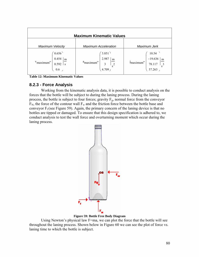
80

Maximum Kinematic Values

Maximum Velocity Maximum Acceleration Maximum Jerk

vmaximum

0.656

0.454

0.592

0.6

⎛⎜⎜⎜⎜⎝

⎞⎟⎟⎟⎟⎠

ms

= amaximum

3.851

2.987

3

4.709

⎛⎜⎜⎜⎜⎝

⎞⎟⎟⎟⎟⎠

m

s2= jmaximum

10.54

19.636−

78.117

57.263

⎛⎜⎜⎜⎜⎝

⎞⎟⎟⎟⎟⎠

m

s3=

Table 12: Maximum Kinematic Values

8.2.3 - Force Analysis Working from the kinematic analysis data, it is possible to conduct analysis on the forces that the bottle will be subject to during the laning process. During the laning process, the bottle is subject to four forces; gravity Fg, normal force from the conveyor FN, the force of the contour wall Fw and the friction force between the bottle base and conveyor Ff (see Figure 59). Again, the primary concern of the laning device is that no bottles are tipped or damaged. To ensure that this design specification is adhered to, we conduct analysis to test the wall force and overturning moment which occur during the laning process.

Figure 59: Bottle Free Body Diagram

Using Newton’s physical law F=ma, we can plot the force that the bottle will see throughout the laning process. Shown below in Figure 60 we can see the plot of force vs. laning time to which the bottle is subject.

81

0 0.05 0.1 0.15 0.2 0.250

2

4

6

8Force on Bottle

Contour Contact Time (s)

Forc

e (N

ewto

ns)

Fwall aheuft tsplit,( )Fwall asin tsplit,( )Fwall atrap tsplit,( )Foptimal tsplit Cout,( )Ffriction

tsplit

Figure 60: Force on Bottle Notice that the curves are shaped the same as the acceleration curve because the mass of the bottle is constant in all four cases. Also, notice the solid horizontal cyan force of friction line. This is the force of static friction between the bottle and conveyor (as the bottle is assumed stationary relative to the conveyor, no slip) and represents the point at which static friction switches to kinetic friction. The static friction force is the maximum force that the bottle will experience opposing the force of the wall. The bottle will not begin traversing the conveyor laterally until the force from the wall exceeds the force of static friction. It is desirable to exceed this force as rapidly as possible, as is done in the mod trap profile.

82

8.2.4 - Moment Analysis Through the force analysis, the overturning moment can be analyzed, assuming a

height at which the contour contacts the bottle. Figure 61 shows the moment plots and again are similar in shape to the acceleration plot.

0 0.05 0.1 0.15 0.2 0.250

0.2

0.4

0.6Induced Moment on Bottles

Contour Contact Time (s)

Mom

ent (

N-m

)

Mwall aheuft tsplit, hcontact,( )Mwall asin tsplit, hcontact,( )Mwall atrap tsplit, hcontact,( )Moptimal tsplit Cout, hcontact,( )Mg

tsplit

Figure 61: Induced Moment on Bottles The horizontal cyan line shown in the plot is the moment sufficient to cause the bottle to begin to tip. We can understand this baseline moment calculation by examining Figure 59. Assuming that Fg acts at the center of gravity (CG), this point force induces a moment about the bottom corner of the bottle with the bottle radius as the moment arm. The plots are simply the force of the wall multiplied by the height at which the wall contacts the bottle. If this moment is greater than that caused by gravity, the bottle will begin to tip.

Notice that the polynomial function crosses the tipping mark, meaning this particular contour could have the potential to cause instability in the bottle. The other two contours in question both induce lower maximum moments than the current Heuft system.

83

Table 13 shows the maximum force and moment of each contour. The order is the same used in all of the plots: Heuft, Simple Harmonic, Mod Trap, and Polynomial. As we can see from the values, the simple harmonic and mod trap yield similar values that are smaller than the other two contours.

Force Analysis

Maximum Force Maximum Moment

Fmaximum

4.968

3.853

3.87

6.074

⎛⎜⎜⎜⎜⎝

⎞⎟⎟⎟⎟⎠

N= Mmaximum

0.442

0.343

0.344

0.54

⎛⎜⎜⎜⎜⎝

⎞⎟⎟⎟⎟⎠

N m⋅=

Table 13: Maximum Force Analysis Values

8.3 - Trajectory Test The camoid laner is a direct replacement of the Heuft system with no further line or rail manipulation. In order to be certain that the laner will cause the bottles to divert fully into the second lane; the bottle trajectories from the end of the cam contour of the three curves are compared to the Heuft. The trajectories are shown in Figure 62.

0 0.05 0.1 0.15 0.2 0.25 0.3 0.35 0.40

0.1

0.2

0.3

Bottle Trajectory Curve

Trajectory Time (s)

Dis

plac

emen

t (m

) Tc_gen ttraj( )Tc_sin ttraj( )Tc_trap ttraj( )Tc_gen t( )

ttraj

Figure 62: Bottle Trajectories From the figure we can see that the trajectories are very similar, eliminating any worries about the bottle’s following a correct diversion path.

84

8.4 - Choosing a Contour After this analysis, it is possible to choose the contour that will most suit the application which we need. For the purposes of the high speed bottle laner, the Modified Trapezoid (mod trap) contour is chosen based on the following explanations.

8.4.1 - Acceptable Final Velocity The velocity curve of the mod trap closely resembles the current system and provides a similar final velocity, which is essential for the bottle to follow the required trajectory for safe laning.

8.4.2 - Minimizing Maximum Acceleration While the mod trap does not provide the lowest maximum acceleration, it comes in at a close second to the simple harmonic. However, the simple harmonic curve is not applicable because of an unacceptably low final velocity.

8.4.3 - Minimizing Jerk The jerk curve of the mod trap is not the best of the group, however still provides continuous and finite values for jerk which are still within the realms of the other analyzed contours. The higher values for jerk are a worthy exception to make for the satisfactory velocity and acceleration profiles.

8.4.4 - Minimizing Force Examining Table 13, the force induced by the simple harmonic and the mod trap are comparable in magnitude and both significantly lower than the other two contours. Again, because of the mod trap’s more acceptable velocity curve, we choose it as the better choice.

8.4.5 - Minimizing Moment Examining Table 13 again for the moment values, we see a similar trend to the force analysis. The mod trap is chosen over the simple harmonic for the same reasons described above for minimizing force. The polynomial function is not an option as the moment induced by the contour is greater than the tipping moment as seen in Figure 61.

8.5 - Torque Requirements Once the geometry of the cam has been set, it is possible to begin to design the second part of the mechanism which is the timing of the rotation. This timing relies directly on the geometry

8.5.1 - Operating Rotational Velocity If the bottle is traveling at line speed, then the time that it takes to travel the length

of the cam laner is represented by Equation 1. Equation 2 is the calculation for the operating rotational velocity. Equation 3 shows the worst case scenario time between two bottles with a bottle spacing of one bottle diameter center to center of bottles on conveyor.

85

Timing Data

Equation 1: Bottle and Laner Contact Time

tfinalLsplitvline

:=

tfinal 0.239s=

Equation 2: Operational Rotational Velocity

ωop140degtfinal

:=

ωop 97.665rpm=

Equation 3: Worst Case Scenario Time Between Two Bottles

tworstdbottlevline

:= tworst 0.075s=

Table 14: Time Data

8.5.2 - Angular Acceleration Recall that the cam must be at full operating velocity before any bottle

manipulation can occur. The angular acceleration necessary in the case is based on the spin-up time, the time it takes for the servo to accelerate the camoid up to operating velocity, as well as servo limitations. Recall that the geometry of the cam includes a buffer angle that allows servo acceleration. The allowable spin-up time is directly related to the buffer angle, the smaller the buffer angle the faster the spin-up time required. This relationship is represented by Figure 63.

0 0.01 0.02 0.03 0.04 0.05 0.06 0.07 0.080

20

40

60Acceleration Buffer Angle vs. Spin-up Time

Spin-Up Time (s)

Buf

fer A

ngle

(deg

)

βbuffer tspinup( )deg

tspinup

Figure 63: Spin-up time vs. Buffer Angle Notice that the spin-up time is the independent variable. This is because we can find a lower limit on the spin-up time based on servo characteristics and design the camoid buffer angle from there. There is more flexibility in sizing for servo torque than there is in the design of the buffer angle on the camoid.

86

The maximum acceleration of a servo is based on its torque, motor inertia and inertia of the cam. For the purposes of graphical representation, we can specify a lower extreme time of 0 seconds for spin-up. The acceleration plot is based on Equation 4.

Equation 4: Acceleration Function α tspinup( )ωop

tspinup:=

The acceleration plot shown in Figure 64 shows the acceleration necessary to

reach operating velocity for a range of spin-up times. The plot follows intuition as the amount of time allowed to reach a certain velocity increases, the acceleration necessary to reach that velocity increases, in this case, asymptotically.

0 0.01 0.02 0.03 0.04 0.05 0.06 0.07 0.080

5000

1 .104

1.5 .104

2 .104Acceleration vs. Spin-up Time

Spin-Up Time (s)

Acc

eler

atio

n (d

eg/s

^2)

α tspinup( )

tspinup

Figure 64: Acceleration vs. Spin-Up Time

8.5.3 - Torque Required Now that the acceleration profile is plotted, we can specify the torque needed based on the cam and motor mass inertia properties. Equation 5 shows the function used to plot the necessary torque for a desired spin-up time.

Equation 5: Torque Function

Tservo tspinup( ) α tspinup( ) Izz_cam Izz_motor+( )⋅:=

Where: Izz_cam +

Cam Moment of Inertia About

Rotational Axis

Izz_motor) Motor Moment of

Inertia About Rotational Axis

Figure 65 shows the torque vs. spin-up time plot. Notice that it is the same shape

as the acceleration curve.

87

0 0.01 0.02 0.03 0.04 0.05 0.06 0.07 0.080

50

100Servo Torque vs. Spin Up Time

Spin Up Time (s)

Torq

ue (N

-m)

Tservo tspinup( )

tspinup

Figure 65: Servo Torque Required vs. Spin-Up Time This torque graph is rendered for visualization purposes. We will demonstrate in the following section how the motor torque is actually calculated. However, the graph gives a range of what can be expected for the required torques.

8.6 - Stress Analysis Once the maximum torque that will be transmitted is known, we can begin stress analysis on the parts that will experience the most stress. The servo will drive a camshaft which will transmit torque to the camoid by means of a key and keyway. The keyway stress analysis is shown in Table 15. It should be noted that the required torque is based on a spin-up time obtained from the Motion Analysis software, which is the time to accelerate from 0 to operating velocity in the final buffer angle of 7.5 degrees. This time was then input into Equation 5.

88

Keyway Stress Analysis

Key Width Key Length Key Depth Wkey

316

in:=

Lkey 1.5in:= Dkey332

in:=

Equation 6: Shear Force at Key

FshearTmaxDshaft

2

:=

Fshear 684.893N=

Equation 7: Keyway Average Shear Stress

τaveFshearAsec

:=

τave 2.491MPa=

Equation 8: Safety Factor

ηsteelSys_steelτave

:=

ηsteel 50.177=

Where Equation 9: Area of Key Asec Wkey Lkey⋅:=

Equation 10: Required Torque Tmax Tservo .01367s( ):=Required Torque based on Motion

Analysis Tool and MathCAD Torque Plot

Sys_steel 125MPa= Theoretical Yield Strength of Steel Table 15: Keyway Stress Analysis Notice that the safety factor of 50 is adequate for this application.

Stress analysis is conducted on the shaft as shown in Table 16. The torsional deflection and shear stress are the main points of interest for the analysis.

89

Shaft Stress Analysis

Shaft Diameter Shaft Length Material

Dshaft .75in:=

Lshaft 16in= Stainless Steel

Equation 11: Shaft Torsional Deflection

δθshaftTmaxLshaft⋅

Gsteel Jshaft⋅:= δθshaft 0.036deg=

Equation 12: Shaft Shear Stress due to Torsion τshaft

TmaxDshaft

2⋅

Jshaft:=

τshaft 3.172MPa=

Where Equation 13: Shaft Polar Moment of

Inertia Jshaftπ

2

Dshaft2

⎛⎜⎝

⎞⎟⎠

4

⋅:=

Gsteel 216GPa:=

Stainless Steel Modulus of Elasticity

Table 16: Shaft Stress Analysis

8.7 - Fatigue Stress Analysis Because the system will be under cyclic torque loading, it is necessary to conduct fatigue stress analysis which is shown in Table 17. The calculations are conducted for a shaft with a ground surface finish, operating in ambient temperatures, 99% reliability and under non-reversing torsional loading. The corrected fatigue function and safety factor are shown in Equation 14 and Equation 15 respectively.

Shaft Fatigue

Se' 200MPa= Stainless Steel

Uncorrected Endurance Limit

Equation 14: Corrected

Fatigue Function Se Cload Csize⋅ Csurface⋅ Ctemperature⋅ Creliability⋅ Se'⋅:= Se 124.049MPa=

Equation 15: Safety Factor

η torsionSe

τshaft:= η torsion 39.109=

See Appendix M - Detailed Mathematics for detailed information on the mathematics of this section

Table 17: Shaft Fatigue Analysis Notice that the safety factor of 39 is adequate for this application. Inevitably, keyways cause stress concentrations due to the sharp radii of the cut. The stress concentration is based on several factors including notch radius, Neuber’s Constant, and a notch sensitivity factor. The safety factor is calculated based on the yield strength of the stainless steel.

90

Keyway Stress Concentration

Sys_steel 125MPa= Yield Strength of Stainless Steel

Equation 16: Fatigue Stress Concentration Factor

Kfs 1 q Kt 1−( )⋅+:= Kfs 2.442=

Equation 17: Shear Stress Concentration due to Torsion

τconcentration Kfs τshaft⋅:= τconcentration 6.869MPa=

Equation 18: Safety Factor ηkeywaySys_steel

τconcentration:= ηkeyway 18.199=

Table 18: Keyway Stress Concentration Analysis Notice that the safety factor of 18 is adequate for this application.

91

Chapter 9.0 - Prototype Testing This chapter discusses in detail the testing protocol followed for proper data collection on the functionality of the camoid laner prototype. This section is meant to provide the necessary information to successfully duplicate the experiment and record all results.

9.1 - Materials • Test Loop • Camoid Laner

o Camoid o Allen-Bradley MPL - B4520P – MJ22AA servo motor o Alpha SP-100-MF1-10 Gearbox 10:1 ratio o Rockwell Automation Kinetix 3000 Servo Driver o 2x SKF FY ¾ TF Flange Mount Bearings o Lovejoy SE-18 ROSTA Tensioner w/ Hardware o Lovejoy R-15/18 Roller Idler-SE15/18 o Stegmann DG60L WSR 5000 pulse/rev shaft encoder o 2x Goodyear W-28S-H White Eagle Pd (QD Bushed) Sprockets o Martin H ¾ QD Bushing o Martin H 32mm QD Bushing o Goodyear Pd W-720 Eagle Belt o Custom length ¾” keyed stainless steel shaft o Custom chassis design

• 30 test bottles • Data recording device (computer, pen, paper)

9.2 - Objective This test is to ensure no bottles are tipped or damaged during operation, and ensure the repeatability.

9.3 - Variables There are several specific variables that will be tested in order to meet aforementioned objective.

• Bottle Spacing • Number of Bottles per Cycle

9.4 - Setup Safety Precaution Safety is of primary concern when dealing with high voltage applications. In this case, 480 volt electrical inputs are required. Only those qualified and experienced to handle high voltage should do so. Servo motors are very powerful and should be handled with care. DO NOT place any body parts on or near any part of mechanism when power is on. DO NOT stand in path of diverting bottles if servo should malfunction and kick bottles off line.

92

9.5 - Setup All testing will be conducted on the specific test loop that Gallo has set up for testing new instruments shown in Figure 66. This test setup assumes the laner has been mounted to the line.

Figure 66: Test loop A series of tests will be conducted testing the two variables mentioned before. The tests will be set up to find an extreme value at which the mechanism no longer functions correctly. Before the test is conducted, there are several initial parameters of the test that must be discussed.

• Bottle Batches • Test Loop Speed • Photoeye Placement • Electronic Attachment

9.5.1 - Bottle Test Batches Bottle batches are small so that if any problems arise, there is not a catastrophe

with tipped bottles. Batches of six bottles will be used, each bottle labeled 1-6. Also, the bottle spacing can be set easier with smaller batches. Once we know that the settings are correct and tipped bottles are minimized, a stream of bottles can be placed safely on the line.

93

9.5.2 - Test Loop Speed The test loop has a maximum speed of 24 inches per second without overloading the test loop system.

9.5.3 - Photoeye Placement The photoeye is placed directly in front of camoid laner in this case for ease of

programming. The camoid is triggered as soon as the target bottle breaks the photoeye beam. Care must be taken to assure the photoeye is triggered once per bottle. This becomes an issue when the photoeye reads through the transparent bottle body. It is possible to trigger twice; once on the leading edge and once on the trailing edge of the same bottle. To avoid this, the photoeye is placed either at the bottle neck where there is an opaque cork or at the base where the glass is sufficiently thick to block enough of the beam. This test used the latter method.

9.5.4 - Electronic Attachment All electronics are attached to their respective power sources by control engineer David Booth. The electronics board is shown in Figure 67.

Figure 67: Electronics Board

The setup of the control electronics was conducted by David Booth and Brandon Abell of Gallo’s Control engineering department. Information regarding the design of the control schematics and hardware setup will not be discussed in this report. Information this can be researched under the heading motion control. When attaching electronics to 480V power sources, extra care should be taken.

94

9.6 - Procedure Safety Precaution The number of bottles per cycle for the camoid laner should be NO LESS than 4 BOTTLES PER CYCLE. Doing so can result in servo misfiring, potentially kicking bottles off the line at high speed. The first tests conducted with less than four bottles per cycle outlines the steps taken to obtain this safety hazard information.

Again, do not stand in front of the diverting bottles at any time to avoid any potential injury. Any tipped bottles should be removed from the line as fast as possible to avoid misfiring.

9.7 - Procedure The procedural steps for testing are explained below. These steps are followed

only after laner mounted, the servo is programmed, electronics are active, and laner is in its default home position which is in the off position.

1. Set up batch of bottles to be tested with spacing according to test number 1 in the

data recording table (shown in Appendix K – Test Data Table) while line is not running

2. Set up program for bottles per cycle according to the test data table. 3. Turn on conveyors 4. Run test five times – bottle batch loops five times – adjust spacing each time 5. Record results 6. Repeat for each test according to test data table

9.7.1 - Data Recording Any abnormal interactions such as impacts, punches, off timing, diversion due to

incorrect geometry, or any other potential problems will be recorded and explained in the test data table. Each bottle is labeled in the batch and if a bottle falls, the number of the bottle is recorded. This will give insight how the actuation and geometry of the camoid are functioning. In addition to the bottle interaction, a second set of observations is needed to record the functioning of the machine itself and any abnormalities experienced with the mechanics of the cam and actuation. The test protocol will be set up such that any problems encountered will be followed by a set of recommendations on how to improve and/or solve such problems, if the problems cannot be solved by us in the allotted time.

95

Chapter 10.0 - Test Results The results of the testing are discussed in detail in this chapter. Also explained are safety issues and problems experienced during the testing sequence. Conclusions provide a concise explanation of the most important findings. Picture sequence of the testing is shown in Figure 68.

Figure 68: Final Mechanism Cycle Sequence

10.1 - Testing Limitations There are several limitations experienced with the test loop:

1. No available line encoder

96

2. No variable line speed 3. Conveyor Condition 4. Not full line speed

10.1.1 - Line Encoder The test loop did not offer a reliable means to attach a line encoder. This has implications when setting the line speed in the program logic. Since the functionality of the design is reliant on the line speed, outside instruments were used to measure the line speed so that it could be hard coded into the program.

10.1.2 - Variable Line Speed Because the line speed is hard coded in the control program, the line speed must be held constant. This made testing for variable line speed impossible without shutting the line down and adjusting the program logic.

10.1.3 - Conveyor Condition The conveyor condition was poor for the purposes of providing a smooth transition across the lines. In several sections of the conveyors, remnants of adhesives caused increased friction as bottles slide across. The test loop also does not include a lubrication system which also results in increased friction. Furthermore, there was a misalignment between two conveyors causing a small lip on which bottles periodically tipped.

10.1.4 - Line Speed We were not able to set the test loop for full line speed because of the apparent safety hazards that could arise from the poor condition of the conveyors. The line speed was set to 24 inches per second, which translates to roughly 250 bottles per minute.

10.2 - Preliminary Testing The actual testing of the laner was not conducted until it was certain that the

mechanism would function safely. A series of preliminary tests were conducted to ensure safe operation, find the minimum number of bottles per cycle and the placement of the photoeye. Several important results were gathered from the preliminary tests using the current programming logic.

• Minimum number of bottles per cycle is 4 • Photoeye must be placed such that either the base of the bottle of the corked

part of the bottles break the beam The reason for a 4 bottle minimum per cycle lies in the geometry of the camoid

and the timing of the actuation. The camoid length is 9.5 inches, which is approximately 3 bottle diameters. If the camoid is set to actuate in 2 or less bottles, the following sequence of events can occur:

1. Bottle 1 triggers actuation 2. Camoid begins rotating

97

3. Bottle 2 crosses photoeye and begins to be diverted. Camoid is still rotating

4. Bottle 3 crosses photoeye, triggering actuation during camoid rotation This poses a problem because the second actuation is triggered during the first.

Under the current program logic, this caused erratic behavior in the servo. The minimum number of bottles per cycle is set at four to ensure such an event will not occur under any circumstance.

Also under the current program, the photoeye must be placed at the base or neck of the bottle. If it is placed such that its position aligns with the body of the bottle, the beam will be broken twice due to the transparency of some products. This will cause two counts for every one bottle. The current program causes actuation every four counts of the photoeye.

98

10.3 - Results Table The results of the test are shown in Table 19.

Camoid Laner Prototype Test: Bottle Interaction Test Administered by: William Robinson Caruso, James Freeman Saunders, David Booth, Shawn Burns

Date: February 28, 2007

Bottle Type: 7305 Time: 9:00-17:00

Test Num

ber

Line Speed (in/sec)

Bottle Spacing (inches)

Number of

Bottles

Bottles per

Cycle

Down Bottle

# Motion* Comments Recommendations

1 24 0 6 1 all ext.

2 24 1 6 1 all ext.

3 24 2 6 1 all ext.

4 24 3 6 1 all ext.

5 24 0 6 2 all ext.

6 24 1 6 2 all ext.

7 24 2 6 2 all ext.

8 24 3 6 2 all ext.

Failure due to laning trigger while servo is in rotation. This causes servo to

attempt to rotate to position B in the

middle of rotating to position A. This

behavior is erratic and causes downed

bottles.

With current timing program, a minimum of

4 bottles per cycle is required to avoid such

an issue. Program optimization could also

avoid this issue

9 24 0 6 4 3 ext.

10 24 1 6 4 3 ext.

11 24 2 6 4 none ext.

12 24 3 6 4 none ext.

The minimum spacing for this

laner is approximately 2

inches. If the bottles are tighter, the

bottle directly before the target bottle

(bottle #3) is adversely affected.

Geometry and controls optimization can be

conducted to attempt to cause the camoid to fit between tighter spaced

bottles.

13 24 0 6 4 none ret.

14 24 1 6 4 none ret.

15 24 2 6 4 none ret.

The camoid doesn’t have any trouble retracting even at minimum bottle

spacing

16 24 2 24 4 none both All bottles

successfully laned. No problems.

Each test is run 5 times to assure all problems with a batch of 6 bottles looping the test line. *ext. = extension ret. = retraction

Table 19: Test Results

99

There are several key points of interest that can be concluded from the results:

• Minimum bottle spacing for reliable camoid extension: 2 inches • Minimum bottle spacing for reliable camoid retraction: no minimum • Line speed affects the magnitude of displacement of the bottle • Photoeye placement

10.3.1 - Minimum Bottle Spacing: Extension There is a minimum bottle spacing of 2 inches that is required in order for the camoid laner to reliably lane bottles. The potential for tipped bottles increases drastically when the bottles are spaced closer than 2 inches. The bottle that was most often tipped was the last bottle to continue in the default lane, bottle 3 of 6. This occurs because the camoid contacts the bottle during rotation and actively pushed the bottle aside. If the bottles are spaced more than 2 inches, the camoid avoids striking the bottle and rotates successfully between the two bottles.

10.3.2 - Minimum Bottle Spacing: Retraction There is no minimum for bottle spacing during the retraction of the camoid; the bottles can be directly adjacent to one another. No bottles were tipped or subject to abnormal manipulation at any point during the retraction, regardless of the spacing.

10.3.3 - Magnitude of Displacement The line speed directly affects the magnitude of displacement. Successful laning of the camoid relies on the trajectory of the bottle after the end of the camoid. The trajectory is dependent on the velocity of the bottle, which is less in slower line speeds. With slower bottle speeds, the bottle tended not to make the full diversion. This lack of displacement is also due to the decreased magnitude of momentum the bottle possesses to overcome frictional forces. The displacement problem could also be linked to the poor conveyor condition and lack of lubrication.

10.3.4 – Photoeye Placement The servo program is set to trigger as soon as the photoeye is triggered. The best placement for the photoeye for this program proved to be directly on the outside edge of the chassis as close to the conveyor surface as possible. The placement is shown in Figure 69.

Figure 69: Photoeye Placement

100

10.4 - Mechanism Observations Observations about the mechanism concluded no visible wear or fatigue. Furthermore, the mechanism operated smoothly and quietly and offered no impacts due to interference of components.

10.5 - Test Results Conclusions The overall outcome of the testing proved to yield satisfactory results. The original design theory based successful laning on one bottle diameter, or 3 inch, spacing. The test results yield less than the original design concept. Also there is no minimum bottle spacing for the retraction, which also exceeded expectation.

The problem concerning the displacement of the bottles across the line must be addressed. It is expected that under actual line conditions (400 bottles/min, lubricated conveyors) the displacement will act similarly to the Heuft system and fully displace the bottles.

Further testing is essential if the camoid laner is to be implemented for production. However, this test proved that the camoid concept is capable of high speed bottle laning and is candidate for further more rigorous testing.

101

Chapter 11.0 - Cost Comparison The final step in analyzing the camoid laner system is performing a cost analysis of all parts that were used in assembling the system. The following table shows the cost of all parts of the camoid laner compared with the Heuft Delta FW system. For detailed cost analysis and bill of materials refer to Appendix C. Cost Comparison Heuft Camoid

$15,532.32 First Unit (all electronics) $13,000 $9,649.09 Secondary Unit

Table 20: Cost Comparison The cost of the camoid laner is analyzed for several different scenarios as shown in Table 20. The first unit price includes all electronics used for servo motion control, and at $15,500 it is more expensive than the Heuft system. However, the servo electronics make up a significant portion of the total cost. As Gallo implements more servos into production, many of the instruments needed are already on the line being used for other motion control purposes. It is possible to piggyback the camoid laner onto the existing control infrastructure. This reduces the cost significantly as shown by the follow-up unit cost, which utilizes key components that are capable of controlling multiple axes.

If the laner were ever to be used in full production, several cost saving strategies could be administered such as:

• In house chassis manufacture • Camoid price reduction for bulk purchase • Minimizing servo size • Piggyback existing motion control infrastructure If these strategies are used, the original cost could potentially be reduced further. In addition to reducing the capital cost of the laner, a single actuation servo

system offers significant savings in maintenance costs as the number of cycles demanded on the system is within the design specifications of a servo. Also, the camoid system is simple enough to allow easy replacement of components as opposed to the Heuft system which requires replacement of the entire system. For example, if a servo motor required replacement it could be replaced immediately, on the line, provided the part is in stock.

102

Chapter 12.0 - Recommendations Prior to implementing the camoid bottle laner in a production setting several tasks

must be completed:

12.1 - Line Speed Testing Experimentation was hindered by the lack of encoder information on the test

conveyor. As a result, the laner was not tested under full speed line conditions (400 bottle/minute). It was designed specifically to accommodate full speed, and it is possible that the laner will function better at 400 bottle/minute. Additionally, the laner should be further tested reflecting ramping up and ramping down the line speed.

12.2 - Bottle Testing Only one type of bottle was tested, the 7305 750mL bottle. The 7405 model

should theoretically perform worse than the 7305, having a higher, less-stable center of gravity. At the very least, similar tests should be performed on 7405s. Ideally, all bottles that could run on Line 2 would be tested as well.

12.3 - Endurance Testing The longest single run during testing was 20 minutes. Before production

implementation the laner should run constantly for hours. There is no data that suggests that the laner will fail from repetition.

12.4 - Part Acquisition If additional units are desired, parts can be purchased at much lower cost. New

methods for mold fabrication using rapid prototyping now enable small batch injection molding at reasonable cost. A mold could be purchased for future use; subsequent parts would cost significantly less after the investment in a mold. The chassis could also be fabricated in-house, instead of employing an outside contractor. Finally, the servo used in the prototype was recovered from the junk rack, but was significantly larger than necessary. In the future a smaller servo, the MPL-B230P-HJ42AA, could be used, at roughly half the price.

12.5 - Program Optimization Very little was done with optimization of the servo’s controlling logic. Certain

safeguards could be added to the logic to prevent misfires. Also, through the use of an encoder and a programmed delay, the photoeye could be positioned elsewhere upstream.

12.6 - Geometry Optimization The camoid’s geometry could be refined with more tests. Because bottles may

not impact the laner directly on the rail, the first 1-2 inches of the camoid rise contour are frequently missed entirely. The length could therefore be shortened and the maximum rise could be increased slightly. No geometric alterations are necessary for operation, but could result in a smaller laner footprint.

103

Chapter 13.0 - Conclusions Upon completion, the tests demonstrated the camoid laner to be a viable concept, and one that should be investigated further. Several tests have been outlined, to be completed before taking the camoid laner to a production setting. Many of the factors explored in the construction and experimentation of the prototype suggest that it would be a large improvement over the current system. A single-actuated bottle laner could significantly reduce maintenance costs compared to the 12-actuator Heuft Rejecter. Servo driven equipment is more reliable and longer lasting than pneumatic systems. In addition, the camoid laner performs comparably to the Heuft Rejecter under similar conditions.

104

References E&J Gallo Winery. Who We Are. Retrieved January 10th, 2007, from

http://www.ejgallo.com/ Engineers Handbook. Rapid Prototyping: Electron Beam Molding. Retrieved January 26,

2007 from http://www.engineershandbook.com/Rapidprototyping/ebm.htm. Free Patents Online. Patent Analytics and Patent Searching. Retrieved January 8th, 2007.

from www.freepatentsonline.com. Goodyear Industrial. Eagle Pd Industrial Power Transmissions. Retrieved February 10,

2007, from http://www.goodyearindustrialproducts.com/powertransmission/products/pdf/eagle_pd_belt.pdf.

Heuft USA, Inc. Container Rejection Systems. Retrieved January 10th, 2007, from

www.heuft.com. Heuft USA, Inc. Heuft Operator Training. Maintenance Manual. Version 1.0. June 6,

2006. Page 18-21. KHS. Container Conveying Solutions. Retrieved November 19, 2007 from

www.kisters.com/img/pool/1111_Container%20Conveying%20Systems.pdf. Norton, Robert L. Machine Design: An Integrated Approach. Upper Saddle River:

Pearson Prentice Hall, 2006. Norton, Robert L. Design of Machinery. New York: McGraw Hill, 2004. Rockwell Automation. Motion Analyzer Software. Retrieved February 11, 2007 from

www.ab.com/motion/software/motion_analyzer.html Rockwell Automation. Allen Bradley Servo Motors. Retrieved January 10, 2007 from

www.rockwellautomation.com. Stratasys. Case Study. Retrieved January 19, 2007 from

http://www.stratasys.com/uploadedFiles/North_America/Media/PDF%20Beta%20pulley.pdf Toolcraft Plastics Ltd. Explanation Of and Free Help with Stereolithography process.

Retrieved January 19, 2007 from http://www.toolcraft.co.uk/help_stereolithography_process_sla_models.htm

105

Appendices

106

Appendix A - Relevant Patents Title: Apparatus for controlling the path of transportation of articles Document Type and Number: United States Patent 4986407 Link to this Page: http://www.freepatentsonline.com/4986407.html Abstract: An apparatus for controlling the path of transportation of articles comprises a first conveyor belt which delivers the articles to a plurality of second conveyor belt which delivers the articles to a plurality of second conveyor belts arranged in parallel side-by-side relationship which continue the conveyance of the articles. A plurality of deflectors selectively deflect the articles from the first conveyor belt to one of the second conveyor belts. In order to attain an especially compact construction the first conveyor belt extends obliquely over and rests on the second conveyor belts and is a belt of such small thickness that the articles can slide form the first conveyor belt extends obliquely over and rests on the second conveyor belts and is a belt of such small thickness that the articles can slide form the first conveyor belt onto one of the second conveyor belts without the risk of toppling over. The deflectors are arranged on the side of the first conveyor belt facing away form the direction of conveyance of the second conveyor belts. The first conveyor belt can be a steel belt having a thickness between 0.1 to 0.5 mm. Inventors: Heuft, Bernhard Application Number: 294628 Filing Date: 1988-12-07 Publication Date: 1991-01-22

Figure 70: Patent 4,986,407

107

Title: Linear articulated pusher Document Type and Number: United States Patent 4643291 Link to this Page: http://www.freepatentsonline.com/4643291.html Abstract: A pusher mechanism supported on a framework for deflecting objects from a conveyor has a retractable pusher which is mounted for linear movement transversely across the conveyor. A paddle is pivotably attached at its midportion to an outer end of the pusher. A movable link is secured between the framework and an end of the paddle. Due to these paddle connections, controlled linear movement of the pusher will cause the paddle to articulate on the pusher from a rest position to an operating position at which an object is deflected from the conveyor and back to the rest position. Inventors: Counter, Louis F.; Callies, Fritz A.; Lee, Phillip L.; Application Number: 820855 Filing Date: 1986-01-21 Publication Date: 1987-02-17

Figure 71: Patent 4,643,291

108

Title: Means for laterally deflecting articles from a path of travel Document Type and Number: United States Patent 4321994 Link to this Page: http://www.freepatentsonline.com/4321994.html Abstract: An apparatus for laterally deflecting selected articles from a first conveyor to one or more other conveyors comprises either extensible and retractable deflective segments, or gas nozzles whose intensity is adjustable. The deflective segments have tapered front faces which jointly form a smooth deflecting face whose taper increases in the direction of conveyance. The number of segments used depends on the speed component required, and the segments are extended by only a portion of the lateral distance the articles are to cover, the remainder of the distance being covered by the imparted inertia. Alternative embodiments include a deflecting wedge or flap. Inventors: Heuft, Bernhard; Application Number: 141847 Filing Date: 1980-04-21 Publication Date: 1982-03-30

Figure 72: Patent 4,321,994

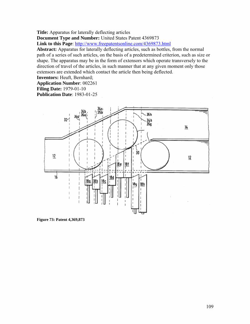
109

Title: Apparatus for laterally deflecting articles Document Type and Number: United States Patent 4369873 Link to this Page: http://www.freepatentsonline.com/4369873.html Abstract: Apparatus for laterally deflecting articles, such as bottles, from the normal path of a series of such articles, on the basis of a predetermined criterion, such as size or shape. The apparatus may be in the form of extensors which operate transversely to the direction of travel of the articles, in such manner that at any given moment only those extensors are extended which contact the article then being deflected. Inventors: Heuft, Bernhard; Application Number: 002261 Filing Date: 1979-01-10 Publication Date: 1983-01-25

Figure 73: Patent 4,369,873

110

Title: Device for singling out articles from a flow of such articles Document Type and Number: United States Patent 6588575 Link to this Page: http://www.freepatentsonline.com/6588575.html Abstract: The device for diverting individual items from a stream of items which are conveyed on a transport apparatus has an extendable and retractable diversion element , which is operated via a gear unit by a drive apparatus moving or swinging to and fro and is precisely time-controllable, in order to impart a cross impulse to items to be diverted so that they slide from the transport apparatus across the direction of transport. The diversion element carries out a complete extension and retraction movement during a single to-or-fro movement or swing of the drive apparatus. The drive apparatus moving to and fro can be a pneumatic cylinder, and the gear unit which transmits the piston movement to the diversion element can be a coulisse link mechanism or a toggle lever. Inventors: Heuft, Bernhard; Kristandt, Gerd; Application Number: 030746 Filing Date: 2001-11-01 Publication Date: 2003-07-08

Figure 74: Patent 6588575

111

Title: Container diverter Document Type and Number: United States Patent 6822181 Link to this Page: http://www.freepatentsonline.com/6822181.html Abstract: The present invention provides a device and method for selectively removing an article from a stream or line of similar articles travelling in a pathway on a transport system such as a conveyor. The invention utilizes a synchronous electric motor which, in response to a signal to reject a specific article in the stream, rotates an article-contacting member or paddle into the path of the stream of articles travelling along the pathway whereby it contacts and smoothly removes that article from the stream. The use of a synchronous motor to effect the rotation of the paddle is very important to the present invention. Inventors: Linton, Fredrick L.; Application Number: 891616 Filing Date: 2001-06-27 Publication Date: 2004-11-23

Figure 75: Patent 6,822,181

112

Title: Side Transfer Sorting Conveyor Document Type and Number: United States Patent 3791518 Link to this Page: http://www.freepatentsonline.com/3791518.html Abstract: A sorting conveyor having a plurality of movable plaques on one conveyor base arranged to sort merchandise or similar articles carried on another conveyor positioned at one side of the sorting conveyor. The separation of articles may be controlled by some particular property of articles such as weight, size, or color, sensed in a known manner. The plaques on the sorting conveyor are activated to engage the articles carried by the adjoining conveyor and change their relative position so that a series of fences can direct the reoriented articles into predetermined paths Inventors: Vanderhoof, Frank B.; Application Number: 355,000 Filing Date: 1973-04-27 Publication Date: 1974-02-12

Figure 76: Patent 3,791,518

113

Appendix B - Rapid Prototyping Quotes A number of quotes were obtained before ordering the rapid prototyped camoid. A number of different RP techniques and companies were surveyed. The SLA option by RPDG was eventually chosen for the fabrication of the camoid. Company Process Material Lead Time Price Discount Final $RPDG SLA ABS-Like 3 days 1219 20 975.2

SLS Nylon 5 days 3888 0 3888FDM ABS-Black 3 days 1612 0 1612FDM PC-White 3 days 1612 0 1612Objet ABS-Like 3 days 2232 0 2232

RedEye RPM FDM PC-ABS Blend 5 days 1500 10 1350Realize SLA Accura 25 5 days 3550 10 3195

114

Appendix C - Bill of Materials Project Budget: Camoid Laner Single Unit

Cost Item Description Part Number Unit Cost QTY Cost Subtotals Camoid SLA Part Cost $1,219.00 1 $1,219.00 20% Discount -$244.00 1 -$244.00

Sales Tax $75.56 1 $75.56 $1,050.56

Allen-Bradley Servo

460V 6.1 N-m 2.3 kW Low Inertia Servo

MPL-B4520P-MJ22AA $1,352.35 1 $1,352.35

Servo Power Cable Power A-B 2090-XXNPMP-

14S05 MTR PWR $98.00 1 $98.00

Servo Feedback Cable Feedback

A-B 2090-UXNFBMP-S05 MOTOR CAB $105.53 1 $105.53

Alpha Gearbox 10:1 Planetary Gearbox $300.00 1 $300.00

PLC Modules $0.00

ControlLogix Chassis 7 Slot ControlLogix Chassis 1756-A7 $291.28 1 $291.28

Ethernet Module

CLX EtherNet/IP 10/100 Bridge Module 1756-ENBT $1,159.84 1 $1,159.84

DC Input Module 10-31 VDC Input 16 Pts (20 Pin) 1756-OB16E $206.27 1 $206.27

DC Output Module

10-31 VDC Elec Fused Output 16 Pts (20 Pin) 1756-OB16E $332.14 1 $332.14

SERCOS Module

3 Axis SERCOS Interface Servo Module 1756-M03SE $751.26 1 $751.26

Module Power Supply

19.2-32 VDC Power Supply (5V @ 10 Amp) 1756-PB72 $530.50 1 $530.50

ControlLogix Processor

Logix5561 Processor With 2Mbyte Memory 1756-L61 $3,364.20 1 $3,364.20

Module, Integrated, 400/460V, 6 kW Conv. 9A Inv 2094-BC01-M01 $1,997.50 1 $1,997.50

SERCOS Fi-Os Cable Fiber Optic Cable $81.00 2 $162.00

Kinetix Ultra3000 Servo Driver 480V AC 3 Phase 2098-DSD-HV050 $1,863.20 1 $1,863.20

Stegmann Shaft Encoder

5000 pulse/rev 6-30V DG60L WSR 5000 $300.00 1 $300.00

Stegmann Encoder Cable 12-Pin Cable

DOL-2312-G03MMA3 $85.00 1 $85.00

Next-Day Shipping $40.00 1 $40.00

Banner PhotoEye PE QS18VP6LPQ5 PE QS18VP6LPQ5 $61.85 1 $61.85

Cable 9m $28.23

Bracket $16.54 1 $16.54

Reflector $5.50 1 $5.50 $13,022.9

6

Drive Sprocket Eagle PD 28-Tooth W-28S-H $52.50 2 $105.00

Drive Belt Eagle Pd 720mm Belt Pd W-720 $35.19 1 $35.19

115

Sprocket Bushings

Martin QD Bushing H-size 3/4 Bore H ¾ QD $9.44 1 $9.44

Martin QD Bushing H-size 32 mm Bore H32 $6.21 1 $6.21

Tax $0.46 1 $0.46

Lovejoy ROSTA Tensioner SE18 Tension Arm SE-18 ROSTA $41.10 1 $41.10

Lovejoy ROSTA Roller Idler Smooth Roller Idler 685144-53028 $34.32 1 $34.32

Tax $2.53 1 $2.53 $234.25

Chassis Labor $507.50 1 $507.50

Parts $576.60 1 $576.60

Tax $78.60 1 $78.60

SKF Bearing 4-Bolt Flange Mount 3/4 Shaft Bearing SKF FY ¾ TF $29.21 2 $58.42

Hardware 1/4-20x1 hex head bolt $0.04 8 $0.32

1/4 split washer $0.02 9 $0.18

1/4-20 Nylock nut $0.04 1 $0.04

5/16-18x1.25 hex head bolt $0.04 4 $0.16

5/16 split washer $0.03 8 $0.24

3/8-16x1 hex head bolt $0.05 8 $0.40

3/8 washer $0.02 8 $0.16

3/8-16 Nylock nut $0.04 8 $0.32

3/4 washer $0.05 4 $0.20

3/16x3/16x1 key $0.02 3 $0.06

3/4 shaft collar $2.35 1 $2.35 $1,225.55

TOTAL $15,533.32 Table 21: Full Bill of Materials

116

Project Budget: Follow-up Cost Item Description Part Number Unit Cost QTY Cost Subtotals Camoid SLA Part Cost $1,219.00 1 $1,219.00

20% Discount -$244.00 1 -$244.00

Sales Tax $75.56 1 $75.56 $1,050.56

Allen-Bradley Servo 460V 6.1 N-m 2.3 kW Low Inertia Servo MPL-B4520P-MJ22AA $1,352.35 1 $1,352.35

Servo Power Cable Power A-B 2090-XXNPMP-

14S05 MTR PWR $98.00 1 $98.00

Servo Feedback Cable Feedback

A-B 2090-UXNFBMP-S05 MOTOR CAB $105.53 1 $105.53

Alpha Gearbox 10:1 Planetary Gearbox $300.00 1 $300.00

PLC Modules $0.00

SERCOS Module 3 Axis SERCOS Interface Servo Module 1756-M03SE $751.26 1 $751.26

Module, Integrated, 400/460V, 6 kW Conv. 9A Inv 2094-BC01-M01 $1,997.50 1 $1,997.50

SERCOS Fi-Os Cable Fiber Optic Cable $81.00 2 $162.00

Kinetix Ultra3000 Servo Driver 480V AC 3 Phase 2098-DSD-HV050 $1,863.20 1 $1,863.20

Stegmann Shaft Encoder 5000 pulse/rev 6-30V DG60L WSR 5000 $300.00 1 $300.00

Stegmann Encoder Cable 12-Pin Cable DOL-2312-G03MMA3 $85.00 1 $85.00

Next-Day Shipping $40.00 1 $40.00

Banner PhotoEye PE QS18VP6LPQ5 PE QS18VP6LPQ5 $61.85 1 $61.85

Cable 9m $28.23

Bracket $16.54 1 $16.54

Reflector $5.50 1 $5.50 $7,138.73

Drive Sprocket Eagle PD 28-Tooth W-28S-H $52.50 2 $105.00

Drive Belt Eagle Pd 720mm Belt Pd W-720 $35.19 1 $35.19

Sprocket Bushings

Martin QD Bushing H-size 3/4 Bore H ¾ QD $9.44 1 $9.44

Martin QD Bushing H-size 32 mm Bore H32 $6.21 1 $6.21

Tax $0.46 1 $0.46

Lovejoy ROSTA Tensioner SE18 Tension Arm SE-18 ROSTA $41.10 1 $41.10

Lovejoy ROSTA Roller Idler Smooth Roller Idler 685144-53028 $34.32 1 $34.32

Tax $2.53 1 $2.53 $234.25

Chassis Labor $507.50 1 $507.50

Parts $576.60 1 $576.60

Tax $78.60 1 $78.60

117

SKF Bearing 4-Bolt Flange Mount 3/4 Shaft Bearing SKF FY ¾ TF $29.21 2 $58.42

Hardware 1/4-20x1 hex head bolt $0.04 8 $0.32

1/4 split washer $0.02 9 $0.18

1/4-20 Nylock nut $0.04 1 $0.04

5/16-18x1.25 hex head bolt $0.04 4 $0.16

5/16 split washer $0.03 8 $0.24

3/8-16x1 hex head bolt $0.05 8 $0.40

3/8 washer $0.02 8 $0.16

3/8-16 Nylock nut $0.04 8 $0.32

3/4 washer $0.05 4 $0.20

3/16x3/16x1 key $0.02 3 $0.06

3/4 shaft collar $2.35 1 $2.35 $1,225.55

TOTAL $9,649.09 Table 22: Bill of Materials with Piggy Backed Electronics

118

Appendix D - Motion Analyzer Input Values Each table represents a tab for the motor sizing application. The software can be downloaded for free at www.ab.com/motion/software/motion_analyzer.html. Axis Setup Load Type Rotary Motor Type Rotary Actuator Type Non-selected Voltage Selection Supply Type AC 3-phase Voltage Type Single Nominal Voltage (volts) 480 Tolerances ±10% Motor Parameters Max ambient (°C) 40 Brake NO Table 23: Axis Setup Tab Cycle profile Cycle Profile mode: Multi-segment Auto Compile: ON Segment Number 1 2 3 4 5 6 7 8 9

Curve Type (Linear/S-curve) L L L L L L L L L

Initial Velocity (deg/sec) 0 0 878.6 878.6 0 0 1098 1098 1174

Final Velocity (deg/sec) 0 878.6 878.6 0 0 1098 1098 1174 0

Distance (deg) 0 32.8 140 7.5 0 7.5 140 10 65.1

Time (sec) 0.413 0.07466 0.07466 0.01707 1.593 0.01367 0.1276 0.008805 0.1109

Acc/Dec (rpm/sec) 0 1961 1961 -8577 0 13380 0 1448 -1764

Thrust (N-m) 0 0 0 0 0 0 0 0 0

Added Inertia (kg-m²) 0 0 0 0 0 0 0 0 0

Denotes an entered value Table 24: Cycle Profile Tab

119

Mechanism Primary Inertia (kg-m²) 0.0059

Secondary Inertia (kg-m²) 0

Secondary Mass (kg) 0

Losses (N-m) 0

Starting Angle (deg) 220

Axis Separation (mm) 0

Table 25: Mechanism Tab

Transmission Stages

Transmission Belt Drive Ratio 10 Inertia (kg-m²) 0.0005 Efficiency 98%

Friction Torque (N-m) 0

Table 26: Transmission Stages Tab

120

Appendix E - Servo Details The following motor descriptions were gathered from Rockwell Automation’s web catalog which can be found at http://literature.rockwellautomation.com/idc/groups/literature/documents/pp/mp-pp001_-en-p.pdf.

Figure 77: Servo Overview

121

122

Appendix F - Servo Driver Details All information gathered from Rockwell Automation Publication http://www.ab.com/motion/controllers/2098-BR002A-EN-P_1001.pdf

Figure 78: Driver Details and Benefits

123

Figure 79: Driver Specifications

124

Figure 80: Driver Specifications

125

Appendix G - Chassis Drawings The following technical drawings were sent to the metalworking contractor. They detail the construction of the chassis components, as well as its assembly. All drawings were made in PTC Pro/ENGINEER Wildfire 2.0. The latest files of each part (PDF, .drw, and .prt files) are included in the electronic version of this report.

126

127

128

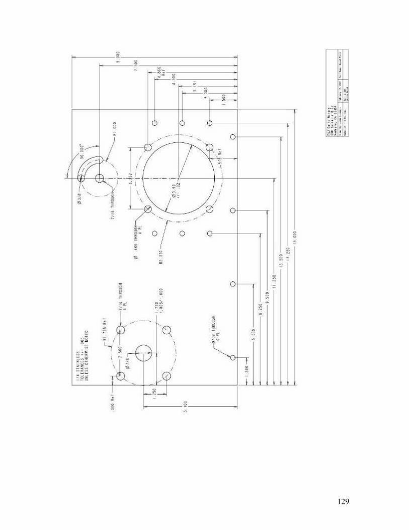
129

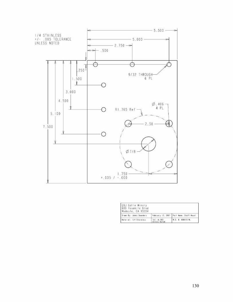
130

131

132

133

Appendix H - Goodyear Eagle Pd Power Transmission

Figure 81: Belt Nomenclature

134

Figure 82: Eagle Pd Belt Product Numbers

135

Figure 83: Sprocket Nomenclature

136

Figure 84: Eagle Pd White Sprockets Screenshots from Goodyear Eagle Pd technical data and product specifications catalog found at: http://www.goodyearindustrialproducts.com/powertransmission/products/pdf/eagle_pd_belt.pdf

137

Figure 85: Belt Nomenclature

138

Figure 86: Eagle Pd Belt Product Numbers

139

Figure 87: Sprocket Nomenclature

140

Figure 88: Eagle Pd White Sprockets

141

Appendix I - Bottle Tests

I.1 - Center of Gravity Test An experiment was conducted to test the center of gravity of a full wine bottle. Figure 89 demonstrates the experiment set up. The center of gravity is measured through the use of a pendulum. The period of a pendulum is a function of the force of gravity and length of the pendulum arm. The relationship is:

2 lTg

π=

Where T is time of one period, l is the length of pendulum from an objects center of gravity, and g is the acceleration due to gravity. By measuring the time of one period we are able to obtain the effective length (from pivot to center of gravity) of the pendulum by rearranging the above relationship:

2

*2Tl gπ

⎡ ⎤= ⎢ ⎥⎣ ⎦

Since we know the dimensions of the bottle and length of the rope we use for the pendulum test, we are able to calculate the location of the center of gravity in relation to the bottle. Assumptions are also made that the bottle is symmetric about two axes such that the center of gravity is in the center of the bottle at some height on the z axis (see Figure 90).

142

Figure 89: Center of Gravity Experiment

143

Figure 90: Free Body Diagram

Figure 90 shows the free body diagram of the bottle during the experiment. FG is the force of gravity acting at the center of gravity. CG is the center of gravity. LR is the length of rope used for the experiment. Leff is the effective length of the pendulum acting at the center of gravity. Several tests were conducted with different lengths of rope. The time was recorded for ten periods to pass. Several runs were conducted for each length of rope. The center of gravity is calculated relative to the base of the bottle. Time was recorded with a computer stop clock accurate to 0.05 seconds. Length was measured with a tape measure accurate to 1/8 inch.

144

Center of Gravity Pendulum Test

Trial String Length

Number of

Periods

Total Time (s)

Period (s)

Effective Length

(in.)

Height from Top

(in.)

Height from

Bottom (in.)

1 32.6 10 20.3 2.0 40.5 7.9 4.4 2 32.6 10 20.3 2.0 40.5 7.9 4.4 3 32.6 10 20.3 2.0 40.5 7.9 4.4 4 27.3 10 18.8 1.9 34.5 7.2 5.0 5 27.3 10 18.8 1.9 34.5 7.2 5.0 6 16.5 10 15.9 1.6 24.7 8.2 4.0 7 16.5 10 16.0 1.6 25.0 8.5 3.7 8 16.5 10 15.9 1.6 24.7 8.2 4.0 9 42.1 10 22.7 2.3 50.4 8.3 3.9 10 42.1 10 22.6 2.3 50.0 7.8 4.4

Average 7.9 4.3

Figure 91: Pendulum Test Results

145

I.2 - Coefficient of Static Friction Test An experiment was conducted to test the coefficient of static friction of a full wine bottle on the two materials commonly used for conveyor systems on the Gallo bottling lines. Figure 92 demonstrates the experiment set up. A section of conveyor links is supported and assured to be level using an inclinometer. The conveyor is lubricated with detergent (glycol based). With the bottle on the conveyor section, the conveyor is inclined until the bottle begins to slide. The angle is measured using the inclinometer.

Figure 92: Coefficient of Static Friction Experiment

146

Figure 93: Free Body Diagram

Figure 93 shows the free body diagram of the bottle during the experiment. FG is the force of gravity acting at the center of gravity. FN is the normal force of the conveyor. FF is the friction force of the conveyor. θ is the angle of the tip of the conveyor. The friction coefficient is obtained by calculating Tan(θ). Two separate tests were conducted with plastic and stainless steel conveyor materials and five trials on each material were conducted.

147

Plastic

Trial Angle (degrees)

Coefficient Static Friction

1 7 0.122784561 2 7 0.122784561 3 7.5 0.131652497 4 6.5 0.113935608 5 7 0.122784561

Average 0.124721109

Stainless Steel

Trial Angle (degrees)

Coefficient Static Friction

1 7 0.122784561 2 7.5 0.131652497 3 7 0.122784561 4 7 0.122784561 5 7.5 0.131652497

Average 0.126331735 Figure 94: Plastic Friction Test

Figure 95: Stainless Steel Friction Test

148

I.3 - Bottle Neck Failure Test An experiment was conducted to test the failure load of the bottle neck using a static load acting at an extreme point on the bottle neck. Figure 96 demonstrates the experiment set up. The bottle overhangs off a solid surface with a rope attached to the bottle neck and a means to supply the force.

Figure 96: Bottle Neck Failure Experiment

149

Figure 97: Free Body Diagram

Figure 97 shows the free body diagram of the bottle during the experiment. The force is provided by weights hanging from a rope attached at the point FL. The bottle is supported by a table at point FT and rotation is prevented by FS acting at the base of the bottle. The moment is calculated at two points of interest; the point at M1 and at the speculated weak point (highest stress concentration factor) at M2.

Bottle Neck Test

Mass (kg) Force

(Newtons) FL

Moment 1 (N-m)

Moment 2 (N-m)

Failure? (yes/no)

4 39.2 4.6 2.3 NO 8 78.5 9.1 4.6 NO

12 117.7 13.7 6.9 NO 20 196.2 22.8 11.6 NO 30 294.3 34.1 17.4 NO

The results of the test concluded that the bottle neck was sufficiently strong to withstand the static load of at least 30 kg. Failure was not achieved because of the lack of equipment and the obvious dangers associated with broken glass.

150

Appendix J - Rapid Prototyping Methods Several different methods of rapid prototyping exist. Each method poses particular benefits and constraints. All use similar basic concepts to construct complex geometry from thin layers. A few available methods are investigated below.

J.1 - Stereolithography (SLA) Stereolithography is the most commonly used rapid prototyping technique and

can produce complex geometries shown in Figure 16. This method uses a screened platform in a reservoir of liquid photopolymer. This liquid hardens when exposed to ultraviolet light. The platform is lowered into the tank of liquid so that only a thin film of the photopolymer (from .125 to .2 mm17) is above its surface. Then an ultraviolet laser traces the cross section, leaving a hardened layer of plastic. The platform then lowers one layer thickness, where a roller spreads the photopolymer to ensure the correct thickness, and the process is repeated. Once the part is finished, the excess liquid is washed off, and the part typically requires a curing operation to harden the photopolymer completely.

Stereolithography is very accurate, but relatively expensive and somewhat slower than some other RP methods. Parts may need support structures during fabrication. Pieces formed with SLA may only be suitable for limited function, as the material is not the most robust or durable. SLA is offered by 3D Systems.

Figure 9818 shows a schematic view of the SLA fabrication process. As the platform is lowered into the tank, the SLA model is formed out of the photopolymer liquid resin by the suspended laser, layer by layer. After the forming process the part must still be finished and cured. SLS and EBM (see below) have similar machine setups, but different reservoir material and, in the case of EBM, an electron beam in place of the laser.

17 Toolcraft Plastics Ltd. Explanation Of and Free Help with Stereolithography process. Retrieved January

19, 2007 from http://www.toolcraft.co.uk/help_stereolithography_process_sla_models.htm 18 Figure retrieved from Toolcraft Plastics Ltd.

Figure 98: SLA Schematic Diagram

151

J.2 - Fused Deposition Modeling (FDM) FDM builds a solid part from a plastic wire that is heated and laid in a bead, layer

upon layer. FDM suffers slightly less accuracy than stereolithography, but offers greater flexibility in materials. Available materials include polycarbonate and ABS plastic, which are durable enough to be used not only as prototypes, but even in full production settings. One manufacturer replaced a pulley on an industrial belt sander on its production line with an FDM formed part when the aluminum piece failed. The rapid prototyped piece lasted over one month in full production19. This process is owned by Stratasys, Inc.

J.3 - Selective Laser Sintering (SLS) SLS uses a bed of powder, which may be plastic, ceramic or metal in a similar

manner as stereolithography uses photopolymer liquid. The powder is spread evenly across a piston head and then sintered with a laser to form. The piston lowers and the process is repeated.

SLS pieces are less accurate than those formed with stereolithography, but have no need for support structures or secondary curing. In addition, SLS allows for a great variety of materials to be used. Sintering does result in porous parts, and may require an infiltration process to improve the material properties of the part. Some larger pieces may require up to two days of cooling after the sintering process.

J.4 - Electron Beam Melting (EBM) A newer development in rapid prototyping is Electron Beam Melting. The process is very similar to SLS, but instead of a laser, an electron beam fully melts the powder. The result is a fully homogenous non-porous part, typically made of titanium. The piece requires no secondary operations, but is suitable for any conventional finish process, including heat treatment. Build layers are quite accurate, having a thickness from 0.05 to 0.2 mm20. The process is roughly five times faster than SLS and up to ten times as efficient. This is because the laser used in SLS is largely reflected from the powder surface, while the electron beam has much higher absorption. Stratasys offers EBM machines in North America.

19 Stratasys. Case Study. Retrieved January 19, 2007 from

http://www.stratasys.com/uploadedFiles/North_America/Media/PDF%20Beta%20pulley.pdf 20 Engineers Handbook. Rapid Prototyping: Electron Beam Molding. Retrieved January 26, 2007 from

http://www.engineershandbook.com/Rapidprototyping/ebm.htm.

152

Appendix K – Test Data Table

Table 27: Data Recording Table

153

Appendix M - Detailed Mathematics

SummaryThis analysis serves several purposes. First of all, we are looking to find an "optimal" contour for the cam ofour divider. This requires a look at the accelerations and forces that will arise from shifting this bottle acrossthe lane. Secondly, we want to find the height (z-direction) at which our divider should contact the bottle, inorder to prevent tipping. Finally, a look at the forces, stresses, and impacts involved with the splitting motion isnecessary to ensure that bottles will not be broken.

There are two approaches to defining the contour of this laner. The first is the Bottom-Up method; describe they-value (height) of the bottle as it moves downstream, and then to perform acceleration and force analyses todetermine if the contour is acceptable. Alternately, with the Top-Down method the acceleration curve can bedescribed first, and the contour follows from there.

We have used both methods in this analysis. For instance, the Simple Harmonic Contour is an example of theBottom-Up method, while ModTrap is an example of Top-Down.

Problem Definition

Constants:

g 9.807m

s2

tan 7 deg( ) 0.123

Bottle Properties:

mbottle 1.29 kg Bottle Mass dbottle 2.982 in Diameter of Bottle

thickness .125 in Glass Thickness Fg mbottle g Weight of Bottle

hbottle 12.25 in Bottle Height Fg 12.651 N

hcg 4.33 in Center of Gravity Height

Ixx

mbottle 3dbottle

2

2

hbottle2

12 Ixx 0.011 kg m

2 Iyy Ixx

These are very rough estimates, assuming a solid,uniform density cylinder.

Izz mbottle

dbottle

2

2

2 Izz 9.251 10

4 kg m

2

Line Properties:

vline 1.01m

s Conveyor Velocity

Design Parametersvline 39.764

in

s

Laner Properties:

hcontact 3.5 in Height at which the laner contacts the bottle

h Z( ) Z hcg Distance from contact point to center of gravity

Lsplit 9.5 in Total length of the laner track

hy 2.72 in Target "height" (across the conveyor)

Time Calculations:

tfinal

Lsplit

vline Time to lane one bottle (guided by contour)

tfinal 0.239 s

tsplit 0 s 0.0025 s tfinal

X-Direction Travel:

x t( ) vline t

0 0.05 0.1 0.15 0.2 0.250

0.1

0.2

x tsplit

tsplit

We make the assumption that the bottle speed moving downstream remains essentially constant. Thedivider will actually slow the bottle, but we argue the loss in speed will be insignificant.

Heuft Laner Acceleration

In order to gain a baseline understanding of the accelerations the bottle experiences currently, we will analyze thecontour of the Heuft laning system. The analysis is conducted by plotting points along the contour and calculating forthe best fit trend line. In this case, a cubic equation was chosen with root mean square value of .9999 (99.99%accuracy).

yheuft t( ) .0011 .0254( )x t( )

in

3

.0166 .0254( )x t( )

in

2

.0362 .0254( )x t( )

in .0007 .0254( )

m

0 0.05 0.1 0.15 0.2 0.250.05

0

0.05

0.1

yheuft tsplit

tsplit yheuft tfinal 2.784 in

vheuft t( )tyheuft t( )d

d

0 0.05 0.1 0.15 0.2 0.250

0.5

1

vheuft tsplit

tsplit

aheuft t( )2

tyheuft t( )d

d

2

0 0.05 0.1 0.15 0.2 0.251

2

3

4

aheuft tsplit

tsplit

Laner Contour:

The contour of our rail can be modeled as a 4-5-6-7 cam polynomial funtion of time with a series ofcoefficients. We set a series of boundary conditions to solve for the necessary contour.

ygeneral t C( ) C0

C1

t

s C

2t

s

2

C3

t

s

3

C4

t

s

4

C5

t

s

5

C6

t

s

6

C7

t

s

7

y'general t C( ) C1

2 C2

t

s 3 C

3

t

s

2

4 C4

t

s

3

5 C5

t

s

4

6 C6

t

s

5

7 C7

t

s

6

y''general t C( ) 2 C2

6 C3

t

s 12 C

4

t

s

2

20 C5

t

s

3

30 C6

t

s

4

42 C7

t

s

5

y'''general t C( ) 6 C3

24 C4

t

s 60 C

5

t

s

2

120 C6

t

s

3

210 C7

t

s

4

This matrix is a series of guess coefficients for the solver todetermine our actual coefficients.

Cgeneral

1

1

1

1

1

1

1

1

hy

Boundary Conditions

Given These conditions are selected to minimize the risk of dangerous dynamicsin the lane splitting.

Initial ConditionsFinal Conditions

0 ygeneral 0 Cgeneral =hy ygeneral tfinal Cgeneral =

0 y'general 0 Cgeneral =.6m y'general tfinal Cgeneral =

0 y''general 0 Cgeneral =0 y''general tfinal Cgeneral =

0m y'''general 0 Cgeneral =0m y'''general tfinal Cgeneral =

Cout Find Cgeneral

Cout

0

0

0

0

3.237 103

1.077 104

7.965 103

4.582 104

in This set of coefficients describes our contour as an 8 termpolynomial equation.

0 0.05 0.1 0.15 0.2 0.250.02

0

0.02

0.04

0.06

0.08

ygeneral tsplit Cout flip

hy

tsplit

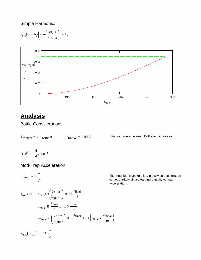
Simple Harmonic:

ysin t( ) hy cosx t( )

2Lsplit

hy

0 0.05 0.1 0.15 0.2 0.250

0.02

0.04

0.06

0.08

ysin tsplit flip

hy

tsplit

AnalysisBottle Considerations:

Ffriction mbottle g Ffriction 1.553 N Friction Force between Bottle and Conveyor

asin t( )2

tysin t( )d

d

2

Mod-Trap Acceleration

amax 3m

s2

The Modified Trapezoid is a piecewise accelerationcurve; partially sinusoidal and partially constantacceleration.

atrap t( ) amax sin2t m

Lsplit s

ttfinal

4if

amax

tfinal

4t 3

tfinal

4if

amax sin2t m

Lsplit s

3tfinal

4 t tfinal

2tfinal

10

if

atrap tfinal 0.187m

s2

Acceleration Comparison

awall a t( ) a t( )

0 0.05 0.1 0.15 0.2 0.250

2

4

6

Bottle Transverse Acceleration

Contour Contact Time (s)

Acc

eler

atio

n (m

/s^2

)

awall aheuft tsplit awall asin tsplit awall atrap tsplit y''general tsplit Cout

tsplit

Velocity

vwall a t( )0

t

ta t( )

d

0 0.05 0.1 0.15 0.2 0.250

0.2

0.4

0.6

0.8

Bottle Transverse Velocity

Contour Contact Time (s)

Bot

tle

Vel

ocit

y (m

/s)

vheuft tsplit vwall asin tsplit vwall atrap tsplit y'general tsplit Cout

tsplit

vfinal

vheuft tfinal vwall asin tfinal vwall atrap tfinal

y'general tfinal Cout s

vfinal

0.656

0.454

0.592

0.6

m

s vfinal

25.824

17.884

23.313

23.622

in

s

Displacement

swall a t( )

0

t

t0

t

ta t( )

d

d

0 0.05 0.1 0.15 0.2 0.250.02

0

0.02

0.04

0.06

0.08

Contour Displacement Profile

Contour Contact Time (s)

Con

tour

Pro

file

yheuft tsplit swall asin tsplit swall atrap tsplit ygeneral tsplit Cout hy

tsplit

sfinal

yheuft tfinal swall asin tfinal swall atrap tfinal

ygeneral tfinal Cout

sfinal

0.071

0.069

0.07

0.069

m sfinal

2.784

2.72

2.758

2.72

in

Displacement Comparison

diffsin tsplit yheuft tsplit swall asin tsplit

difftrap tsplit yheuft tsplit swall atrap tsplit

diffpoly tsplit yheuft tsplit ygeneral tsplit Cout

0 0.05 0.1 0.15 0.2 0.250.2

0

0.2

Displacement Difference: Heuft vs. Cam Programs

Contour Contact Time (s)

Dis

plac

emen

t Dif

fere

nce

(in)

diffsin tsplit in

difftrap tsplit in

diffpoly tsplit in

tsplit

Jerk

In addition to acceleration, velocity, and displacement, we can look at the jerk over the division.

jwall a t( )ta t( )d

d

0 0.05 0.1 0.15 0.2 0.25100

50

0

50

100

Bottle Transverse Jerk

Contour Contact Time (s)

Jerk

(m

/s^3

)

jwall aheuft tsplit jwall asin tsplit jwall atrap tsplit y'''general tsplit Cout

tsplit

Force

Fwall a t( ) a t( ) mbottle Foptimal tsplit Cout y''general tsplit Cout mbottle

0 0.05 0.1 0.15 0.2 0.250

2

4

6

8

Force on Bottle

Contour Contact Time (s)

For

ce (

New

tons

)

Fwall aheuft tsplit Fwall asin tsplit Fwall atrap tsplit Foptimal tsplit Cout Ffriction

tsplit

Contour Comparison TableThe following table compares the peak values of velocity, acceleration and jerk of the contour curves. This willinfluence the decision when choosing the optimal contour for the cam.

Max Velocity Max Acceleration

vmaximum

vheuft tfinal vwall asin tfinal vwall atrap tfinal

y'general tfinal Cout s

amaximum

aheuft tfinal asin 0( )

atrap .1s( )

y''general

tfinal

2Cout

s2

vmaximum

0.656

0.454

0.592

0.6

m

s vmaximum

25.824

17.884

23.313

23.622

in

s amaximum

3.851

2.987

3

4.709

m

s2

amaximum

151.633

117.581

118.11

185.389

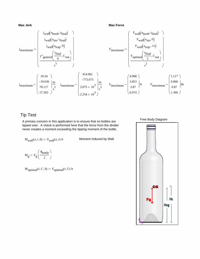
Max Jerk Max Force

jmaximum

jwall aheuft tfinal jwall asin tfinal

jwall atrap 0

y'''general

tfinal

4Cout

s3

Fmaximum

Fwall aheuft tfinal Fwall asin 0

Fwall atrap .1s

Foptimal

tfinal

2Cout

s2

jmaximum

10.54

19.636

78.117

57.263

m

s3

jmaximum

414.961

773.073

3.075 103

2.254 103

in

s3

Fmaximum

4.968

3.853

3.87

6.074

N Fmaximum

1.117

0.866

0.87

1.366

lbf

Tip TestFree Body Diagram

A primary concern in this application is to ensure that no bottles aretipped over. A check is performed here that the force from the dividernever creates a moment exceeding the tipping moment of the bottle.

Mwall a t h( ) Fwall a t( ) h Moment Induced by Wall

Mg Fg

dbottle

2

Moptimal t C h( ) Foptimal t C( ) h

0 0.05 0.1 0.15 0.2 0.250

0.2

0.4

0.6

Induced Moment on Bottles

Contour Contact Time (s)

Mom

ent (

N-m

)

Mwall aheuft tsplit hcontact Mwall asin tsplit hcontact Mwall atrap tsplit hcontact Moptimal tsplit Cout hcontact Mg

tsplit

Maximum Moment

Mmaximum

Mwall aheuft tfinal hcontact Mwall asin 0 hcontact

Mwall atrap .125s hcontact

Moptimal

tfinal

2Cout hcontact

s2

Mmaximum

0.442

0.343

0.344

0.54

N m Mmaximum

3.909

3.031

3.045

4.78

lbf in

Bottle TrajectorySince the contour does not guide the bottle the entire distance across theconveyor, a check is performed to ensure the bottle's trajectory will carry thebottle across the division.

Angle of Trajectory

a t( ) atan0

t

ta t( )

ds

m

gen tsplit Cout atan y'general tsplit

Cout

m

Final Angle of Departure

aheuft tfinal asin tfinal atrap tfinal

gen tfinal Cout

31.772

24.43

30.632

30.964

deg

0 0.05 0.1 0.15 0.2 0.250

10

20

30

40

Angle of Departure

Contour Contact Time (s)

Ang

le (

deg)

aheuft tsplit deg

asin tsplit deg

atrap tsplit deg

gen tsplit Cout deg

tsplit

Bottle Velocity Components

Vx

vline sin 0

vline sin 1

vline sin 2

vline sin 3

Vx

0.532

0.418

0.515

0.52

m

s Vx

20.937

16.445

20.26

20.458

in

s

Vy

vline cos 0

vline cos 1

vline cos 2

vline cos 3

Vy

0.859

0.92

0.869

0.866

m

s Vy

33.805

36.204

34.215

34.097

in

s

Bottle Friction Deceleration

afriction

Ffriction

mbottle afriction 1.204

m

s2

Acceleration due to Friction

Line Constants

Lglide 18in Length of Unsupported Trajectory

tfin

Lglide

vline tfin 0.453 s

Time of Trajectory

ttraj 0 s 0.025 s tfin

X Displacement of Bottle of Trajectory (Downline)

xtraj_heuft t( ) Vx0t xtraj_sin t( ) Vx1

t xtraj_trap t( ) Vx2t

xtraj_gen t( ) Vx3t

0 0.05 0.1 0.15 0.2 0.25 0.3 0.35 0.40

0.1

0.2

xtraj_heuft ttraj xtraj_sin ttraj xtraj_trap ttraj xtraj_gen ttraj

ttraj

Y Displacement of Bottle Trajectory (Across Conveyor)

ytraj_heuft t( ) Vy0t .5 afriction t

2 ytraj_trap t( ) Vy2

t .5 afriction t2

ytraj_sin t( ) Vy1t .5 afriction t

2

ytraj_gen t( ) Vy3t .5 afriction t

2

0 0.05 0.1 0.15 0.2 0.25 0.3 0.35 0.40

0.2

ytraj_heuft ttraj ytraj_sin ttraj ytraj_trap ttraj ytraj_heuft ttraj

ttraj

Trajectory Curve

Tc_heuft t( ) xtraj_heuft t( )2

ytraj_heuft t( )2

Tc_trap t( ) xtraj_trap t( )2

ytraj_trap t( )2

Tc_sin t( ) xtraj_sin t( )2

ytraj_sin t( )2

Tc_gen t( ) xtraj_gen t( )2

ytraj_gen t( )2

0 0.05 0.1 0.15 0.2 0.25 0.3 0.35 0.40

0.1

0.2

0.3

Bottle Trajectory Curve

Trajectory Time (s)

Dis

plac

emen

t (m

) Tc_gen ttraj Tc_sin ttraj Tc_trap ttraj Tc_gen t( )

ttraj

Notice that the trajectories of the proposed contours all produce similar trajectories to the Heuft modelcurrently in place. This reduces any concern for the proposed contours' ability to produce a bottle trajectorythat clears the dividing wedge.

Timing

The nature of the cam is such that one half revolution is a full rise cycle of the cam. The cam must complete a fullrise at the same speed of the bottle. Thus the cam must make one half revolution in a minimum t final.

tfinal

Lsplit

vline

tfinal 0.239 s

op140deg

tfinal op 97.665 rpm Operating Angular Velocity

Angular AccelerationThe successful operation of this system is based upon the fact that the system must be binary, i.e. either

on or off. Binary operation is only achieved when the system is at full operating speed during the cam riseactuation. In order to accomplish this, the cam design incorporates a buffer dwell angle to allow for servoacceleration. The buffer dwell angle is based on a spin up time specified. The specified spinup time has a definiterange whose extremities are governed by several criteria. The lower extreme of spinup time is governed by servotorque. The upper extreme is governed by line speed, bottle spacing and cam geometry.

There is often a spacing between the bottles on the line, however it is not unusual for bottles to be directlyadjacent to eachother. In this case, the spacing between the bottles is a bottle diameter. The worst case timebetween the bottles is thus full line speed and one bottle diameter spacing.

tworst

dbottle

vline tworst 0.075 s Worst Case Scenario Spin Up Time

The fastest a servo can accelerate is based on its torque, motor inertia and inertia of the cam. We can specify anarbitrary lower time of 0 for spinup.

op 97.665 rpm tspinup 0.001s .002s tworst

buffer tspinup tspinup op

0 0.01 0.02 0.03 0.04 0.05 0.06 0.07 0.080

20

40

60

Acceleration Buffer Angle vs. Spin-up Time

Spin-Up Time (s)

Buf

fer

Ang

le (

deg)

buffer tspinup deg

tspinup

tspinup op

tspinup

0 0.01 0.02 0.03 0.04 0.05 0.06 0.07 0.080

5000

1 104

1.5 104

tspinup

tspinup

Torque

Izz_cam 18.64lb in2

Izz_cam 5.455 103

s2

m N Cam Moment of Inertia

Izz_motor 3kg cm2

Motor Moment of Inertia

Tservo tspinup tspinup Izz_cam Izz_motor

0 0.01 0.02 0.03 0.04 0.05 0.06 0.07 0.080

20

40

60

Servo Torque vs. Spin Up Time

Spin Up Time (s)

Tor

que

(N-m

)

Tservo tspinup

tspinup

1 103

0.01 0.10.1

1

10

100

Servo Torque vs. Spin Up Time

Spin Up Time (s)

Tor

que

(N-m

)

Tservo tspinup

tspinup

Cam Physical Properties

Mcam 5.332lb Mcam 2.419 kg Mass of Cam

Vcam 122.99 in3

Vcam 2.015 103

cm3

Volume of Cam

Izz_cam 18.64 lb in2

Izz_cam 5.455 103

kg m2

Cam Moment of Ineria about Rotational Axis

Shaft Properties

steel 7.8gm

cm3

Denisty of Steel

Lbearing 1in Bearing Length

Wgear 2in Gear Width

Lshaft Lsplit 2Lbearing Wgear 2.5in Lshaft 16 in Shaft Length

Dshaft .75in Shaft Diameter

Izz_shaft .25 Dshaft

2

4

Izz_shaft 6.465 109

m4

Moment of Inertia

Jshaft

2

Dshaft

2

4

Jshaft 1.293 108

m4

Polar Moment of Inertia

Vshaft Dshaft

2

2

Lshaft Vshaft 115.833 cm3

Volume of Shaft

mshaft steel Vshaft mshaft 0.903 kg Mass of Shaft

Keyway Analysis

Wkey3

16in Width of Key

Lkey 1.5in Length of Key

Dkey3

32in Depth of Key

Syt_ABS 52MPa Tensile Yield Strength of ABS Plastic

Syt_A25 38MPa Tensile Yield Strength of Accura 25 Plastic

Syt_steel 250MPa Tensile Yield Strength of Steel

Shear Stress Analysis

Tmax Tservo .01367 s( ) Tmax 4.306 N m Maximum Torque Transmission

Fshear

Tmax

Dshaft

2

Fshear 452.029 N Shear Force

Asec Wkey Lkey Asec 1.815 104

m2

Cross Sectional Area of Key

ave

Fshear

Asec ave 2.491 MPa Average Torsional Shear Stress

Safety Factor

Sys_ABS 0.5 Syt_ABS Sys_ABS 26 MPa Theoretical Yield Strength

Sys_A25 0.5 Syt_A25 Sys_A25 19 MPa

Sys_steel 0.5 Syt_steel Sys_steel 125 MPa

ABS

Sys_ABS

ave ABS 10.437 Safety Factor

A25

Sys_A25

ave A25 7.627

steel

Sys_steel

ave steel 50.177

Shaft Analysis

Gsteel 216GPa Modulus of Elasticity

shaft

Tmax Lshaft

Gsteel Jshaft shaft 0.036 deg Shaft Torsional Deflection

shaft

Tmax

Dshaft

2

Jshaft shaft 3.172 MPa Torsion Stress in Shaft

Fatigue Failure Analysis

Torsional Fatigue

Sut 400MPa Sut 400 MPa Ultimate Tensile Strength

Se' .5 Sut Se' 200 MPa Uncorrected Endurance Limit

Cload 1 For Torsional Loading

Csize 0.869Dshaft

in

.097

Size Correction

A 4.51 b .265

Csurface ASut

MPa

b

Csurface 0.922 Surface Finish Correction

Ctemperature 1.0 Ambient Temperature Correction

Creliability .753 Material Reliability Correction

Se Cload Csize Csurface Ctemperature Creliability Se' Corrected Fatigue Function

Se 124.049 MPa

Safety Factor

torsion

Se

shaft torsion 39.109

Keyway Stress Concentration Factors

a 0.039 a 0.0392

Neuber's Constant

r .01 Notch Radius

q1

1a

r

Notch Sensitivity Factor

Kt 2.62 Static Stress Concentration FactorPeterson stress concentration factor for flat endmill. (furlong lecture 19, machine design 473)

Kfs 1 q Kt 1 Kfs 2.165 Fatigue Stress Concentration Factor

Shear Stress Concentration due to Torsion

concentration Kfs shaft concentration 6.869 MPa

Safety Factor

keyway

Sys_steel

concentration keyway 18.199