Bornhuetter--Ferguson as a General Principle of Loss Reserving · Bornhuetter–Ferguson as a...
133
ROT DP oBF eBF SC BFP Ex Ref Bornhuetter–Ferguson as a General Principle of Loss Reserving Klaus D. Schmidt & Mathias Zocher Lehrstuhl für Versicherungsmathematik Technische Universität Dresden ASTIN Conference Manchester, July 14–16, 2008 Klaus D. Schmidt – Bornhuetter–Ferguson ASTIN Manchester, July 14–16, 2008
Transcript of Bornhuetter--Ferguson as a General Principle of Loss Reserving · Bornhuetter–Ferguson as a...

ROT DP oBF eBF SC BFP Ex Ref
Bornhuetter–Ferguson as aGeneral Principle of Loss Reserving
Klaus D. Schmidt & Mathias Zocher
Lehrstuhl für VersicherungsmathematikTechnische Universität Dresden
ASTIN ConferenceManchester, July 14–16, 2008
Klaus D. Schmidt – Bornhuetter–Ferguson ASTIN Manchester, July 14–16, 2008
ROT DP oBF eBF SC BFP Ex Ref
Table of Contents
Run–Off Triangles of Cumulative Losses
Development Patterns
The original Bornhuetter–Ferguson Method
The extended Bornhuetter–Ferguson Method
Special CasesThe Loss–Development MethodThe Chain–Ladder MethodThe Cape Cod MethodThe Additive Method
The Bornhuetter–Ferguson Principle
An Example
References
Klaus D. Schmidt – Bornhuetter–Ferguson ASTIN Manchester, July 14–16, 2008
ROT DP oBF eBF SC BFP Ex Ref
Run–Off Triangles of Cumulative Losses (1)
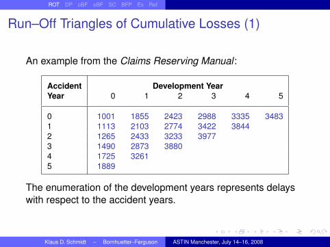
An example from the Claims Reserving Manual :
Accident Development YearYear 0 1 2 3 4 5
0 1001 1855 2423 2988 3335 34831 1113 2103 2774 3422 38442 1265 2433 3233 39773 1490 2873 38804 1725 32615 1889
The enumeration of the development years represents delayswith respect to the accident years.
Klaus D. Schmidt – Bornhuetter–Ferguson ASTIN Manchester, July 14–16, 2008

ROT DP oBF eBF SC BFP Ex Ref
Run–Off Triangles of Cumulative Losses (2)
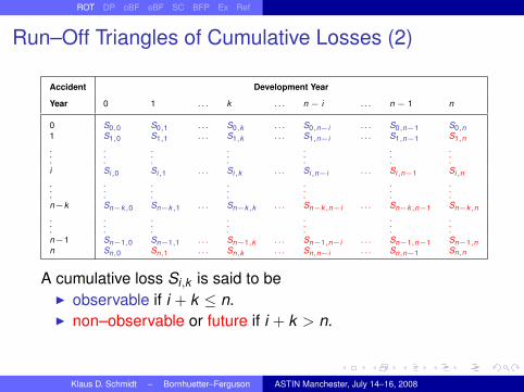
Accident Development Year
Year 0 1 . . . k . . . n − i . . . n − 1 n
0 S0,0 S0,1 . . . S0,k . . . S0,n−i . . . S0,n−1 S0,n1 S1,0 S1,1 . . . S1,k . . . S1,n−i . . . S1,n−1 S1,n...
.
.
....
.
.
....
.
.
....
i Si,0 Si,1 . . . Si,k . . . Si,n−i . . . Si,n−1 Si,n...
.
.
....
.
.
....
.
.
....
n−k Sn−k,0 Sn−k,1 . . . Sn−k,k . . . Sn−k,n−i . . . Sn−k,n−1 Sn−k,n...
.
.
....
.
.
....
.
.
....
n−1 Sn−1,0 Sn−1,1 . . . Sn−1,k . . . Sn−1,n−i . . . Sn−1,n−1 Sn−1,nn Sn,0 Sn,1 . . . Sn,k . . . Sn,n−i . . . Sn,n−1 Sn,n
A cumulative loss Si,k is said to be
I observable if i + k ≤ n.I non–observable or future if i + k > n.I current if i + k = n.I ultimate if k = n.
Klaus D. Schmidt – Bornhuetter–Ferguson ASTIN Manchester, July 14–16, 2008

ROT DP oBF eBF SC BFP Ex Ref
Run–Off Triangles of Cumulative Losses (2)
Accident Development Year
Year 0 1 . . . k . . . n − i . . . n − 1 n
0 S0,0 S0,1 . . . S0,k . . . S0,n−i . . . S0,n−1 S0,n1 S1,0 S1,1 . . . S1,k . . . S1,n−i . . . S1,n−1 S1,n...
.
.
....
.
.
....
.
.
....
i Si,0 Si,1 . . . Si,k . . . Si,n−i . . . Si,n−1 Si,n...
.
.
....
.
.
....
.
.
....
n−k Sn−k,0 Sn−k,1 . . . Sn−k,k . . . Sn−k,n−i . . . Sn−k,n−1 Sn−k,n...
.
.
....
.
.
....
.
.
....
n−1 Sn−1,0 Sn−1,1 . . . Sn−1,k . . . Sn−1,n−i . . . Sn−1,n−1 Sn−1,nn Sn,0 Sn,1 . . . Sn,k . . . Sn,n−i . . . Sn,n−1 Sn,n
A cumulative loss Si,k is said to beI observable if i + k ≤ n.I non–observable or future if i + k > n.I current if i + k = n.I ultimate if k = n.
Klaus D. Schmidt – Bornhuetter–Ferguson ASTIN Manchester, July 14–16, 2008
ROT DP oBF eBF SC BFP Ex Ref
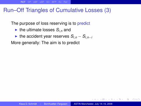
Run–Off Triangles of Cumulative Losses (3)
The purpose of loss reserving is to predictI the ultimate losses Si,n andI the accident year reserves Si,n − Si,n−i
More generally: The aim is to predict
I the future cumulative losses Si,k
I the future incremental losses Zi,k := Si,k − Si,k−1
I the calendar year reserves∑n
j=p−n Zj,p−j
I the total reserve∑n
j=1∑n
l=n−j+1 Zj,l
with i + k ≥ n + 1 and p = n + 1, . . . , 2n.
Thus: The principal task considered here is to predict the futurecumulative losses.
Klaus D. Schmidt – Bornhuetter–Ferguson ASTIN Manchester, July 14–16, 2008
ROT DP oBF eBF SC BFP Ex Ref
Run–Off Triangles of Cumulative Losses (3)
The purpose of loss reserving is to predictI the ultimate losses Si,n andI the accident year reserves Si,n − Si,n−i
More generally: The aim is to predictI the future cumulative losses Si,k
I the future incremental losses Zi,k := Si,k − Si,k−1
I the calendar year reserves∑n
j=p−n Zj,p−j
I the total reserve∑n
j=1∑n
l=n−j+1 Zj,l
with i + k ≥ n + 1 and p = n + 1, . . . , 2n.
Thus: The principal task considered here is to predict the futurecumulative losses.
Klaus D. Schmidt – Bornhuetter–Ferguson ASTIN Manchester, July 14–16, 2008

ROT DP oBF eBF SC BFP Ex Ref
Run–Off Triangles of Cumulative Losses (3)
The purpose of loss reserving is to predictI the ultimate losses Si,n andI the accident year reserves Si,n − Si,n−i
More generally: The aim is to predictI the future cumulative losses Si,k
I the future incremental losses Zi,k := Si,k − Si,k−1
I the calendar year reserves∑n
j=p−n Zj,p−j
I the total reserve∑n
j=1∑n
l=n−j+1 Zj,l
with i + k ≥ n + 1
and p = n + 1, . . . , 2n.
Thus: The principal task considered here is to predict the futurecumulative losses.
Klaus D. Schmidt – Bornhuetter–Ferguson ASTIN Manchester, July 14–16, 2008

ROT DP oBF eBF SC BFP Ex Ref
Run–Off Triangles of Cumulative Losses (3)
The purpose of loss reserving is to predictI the ultimate losses Si,n andI the accident year reserves Si,n − Si,n−i
More generally: The aim is to predictI the future cumulative losses Si,k
I the future incremental losses Zi,k := Si,k − Si,k−1
I the calendar year reserves∑n
j=p−n Zj,p−j
I the total reserve∑n
j=1∑n
l=n−j+1 Zj,l
with i + k ≥ n + 1 and p = n + 1, . . . , 2n.
Thus: The principal task considered here is to predict the futurecumulative losses.
Klaus D. Schmidt – Bornhuetter–Ferguson ASTIN Manchester, July 14–16, 2008

ROT DP oBF eBF SC BFP Ex Ref
Run–Off Triangles of Cumulative Losses (3)
The purpose of loss reserving is to predictI the ultimate losses Si,n andI the accident year reserves Si,n − Si,n−i
More generally: The aim is to predictI the future cumulative losses Si,k
I the future incremental losses Zi,k := Si,k − Si,k−1
I the calendar year reserves∑n
j=p−n Zj,p−j
I the total reserve∑n
j=1∑n
l=n−j+1 Zj,l
with i + k ≥ n + 1 and p = n + 1, . . . , 2n.
Thus: The principal task considered here is to predict the futurecumulative losses.
Klaus D. Schmidt – Bornhuetter–Ferguson ASTIN Manchester, July 14–16, 2008
ROT DP oBF eBF SC BFP Ex Ref
Table of Contents
Run–Off Triangles of Cumulative Losses
Development Patterns
The original Bornhuetter–Ferguson Method
The extended Bornhuetter–Ferguson Method
Special CasesThe Loss–Development MethodThe Chain–Ladder MethodThe Cape Cod MethodThe Additive Method
The Bornhuetter–Ferguson Principle
An Example
References
Klaus D. Schmidt – Bornhuetter–Ferguson ASTIN Manchester, July 14–16, 2008

ROT DP oBF eBF SC BFP Ex Ref
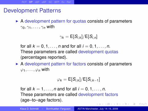
Development Patterns
I A development pattern for quotas consists of parametersγ0, γ1, . . . , γn with
γk = E[Si,k ]/E[Si,n]
for all k = 0, 1, . . . , n and for all i = 0, 1, . . . , n.These parameters are called development quotas(percentages reported).
I A development pattern for factors consists of parametersϕ1, . . . , ϕn with
ϕk = E[Si,k ]/E[Si,k−1]
for all k = 1, . . . , n and for all i = 0, 1, . . . , n.These parameters are called development factors(age–to–age factors).
Klaus D. Schmidt – Bornhuetter–Ferguson ASTIN Manchester, July 14–16, 2008
ROT DP oBF eBF SC BFP Ex Ref
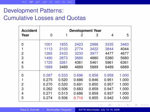
Development Patterns:Cumulative Losses and Quotas
Accident Development YearYear 0 1 2 3 4 5
0 1001 1855 2423 2988 3335 34831 1113 2103 2774 3422 3844 40442 1265 2433 3233 3977 4477 46773 1490 2873 3880 4880 5380 56804 1725 3261 4361 5461 5961 63615 1889 3489 4889 5889 6489 6889
0 0.287 0.533 0.696 0.858 0.958 1.0001 0.275 0.520 0.686 0.846 0.951 1.0002 0.270 0.520 0.691 0.850 0.957 1.0003 0.262 0.506 0.683 0.859 0.947 1.0004 0.271 0.513 0.686 0.859 0.937 1.0005 0.274 0.506 0.710 0.855 0.942 1.000
Klaus D. Schmidt – Bornhuetter–Ferguson ASTIN Manchester, July 14–16, 2008

ROT DP oBF eBF SC BFP Ex Ref
Development Patterns:Cumulative Losses and Factors
Accident Development YearYear 0 1 2 3 4 5
0 1001 1855 2423 2988 3335 34831 1113 2103 2774 3422 3844 40442 1265 2433 3233 3977 4477 46773 1490 2873 3880 4880 5380 56804 1725 3261 4361 5461 5961 63615 1889 3489 4889 5889 6489 6889
0 1.853 1.306 1.233 1.116 1.0441 1.889 1.319 1.234 1.123 1.0522 1.923 1.329 1.230 1.126 1.0453 1.928 1.351 1.258 1.102 1.0564 1.890 1.337 1.252 1.092 1.0675 1.847 1.401 1.205 1.102 1.062
Klaus D. Schmidt – Bornhuetter–Ferguson ASTIN Manchester, July 14–16, 2008
ROT DP oBF eBF SC BFP Ex Ref
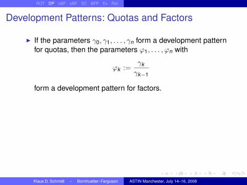
Development Patterns: Quotas and Factors
I If the parameters γ0, γ1, . . . , γn form a development patternfor quotas, then the parameters ϕ1, . . . , ϕn with
ϕk :=γk
γk−1
form a development pattern for factors.
I If the parameters ϕ1, . . . , ϕn form a development patternfor factors, then the parameters γ0, γ1, . . . , γn with
γk :=n∏
l=k+1
1ϕl
form a development pattern for quotas.
Klaus D. Schmidt – Bornhuetter–Ferguson ASTIN Manchester, July 14–16, 2008

ROT DP oBF eBF SC BFP Ex Ref
Development Patterns: Quotas and Factors
I If the parameters γ0, γ1, . . . , γn form a development patternfor quotas, then the parameters ϕ1, . . . , ϕn with
ϕk :=γk
γk−1
form a development pattern for factors.
I If the parameters ϕ1, . . . , ϕn form a development patternfor factors, then the parameters γ0, γ1, . . . , γn with
γk :=n∏
l=k+1
1ϕl
form a development pattern for quotas.
Klaus D. Schmidt – Bornhuetter–Ferguson ASTIN Manchester, July 14–16, 2008
ROT DP oBF eBF SC BFP Ex Ref
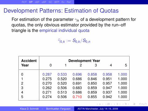
Development Patterns: Estimation of QuotasFor estimation of the parameter γk of a development pattern forquotas, the only obvious estimator provided by the run–offtriangle is the empirical individual quota
γ0,k := S0,k/S0,n
Accident Development YearYear 0 1 2 3 4 5
0 0.287 0.533 0.696 0.858 0.958 1.0001 0.275 0.520 0.686 0.846 0.951 1.0002 0.270 0.520 0.691 0.850 0.957 1.0003 0.262 0.506 0.683 0.859 0.947 1.0004 0.271 0.513 0.686 0.859 0.937 1.0005 0.274 0.506 0.710 0.855 0.942 1.000
Klaus D. Schmidt – Bornhuetter–Ferguson ASTIN Manchester, July 14–16, 2008
ROT DP oBF eBF SC BFP Ex Ref
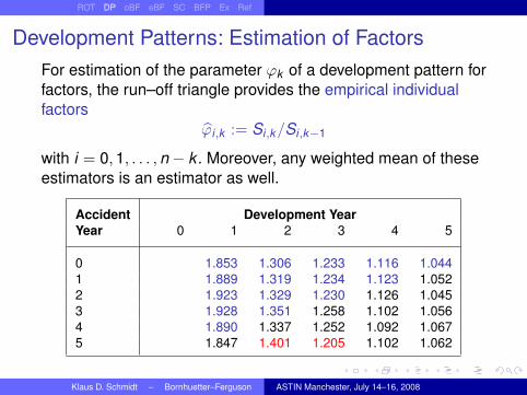
Development Patterns: Estimation of FactorsFor estimation of the parameter ϕk of a development pattern forfactors, the run–off triangle provides the empirical individualfactors
ϕi,k := Si,k/Si,k−1
with i = 0, 1, . . . , n − k . Moreover, any weighted mean of theseestimators is an estimator as well.
Accident Development YearYear 0 1 2 3 4 5
0 1.853 1.306 1.233 1.116 1.0441 1.889 1.319 1.234 1.123 1.0522 1.923 1.329 1.230 1.126 1.0453 1.928 1.351 1.258 1.102 1.0564 1.890 1.337 1.252 1.092 1.0675 1.847 1.401 1.205 1.102 1.062
Klaus D. Schmidt – Bornhuetter–Ferguson ASTIN Manchester, July 14–16, 2008
ROT DP oBF eBF SC BFP Ex Ref
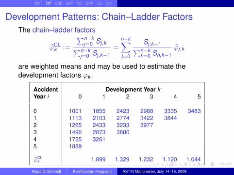
Development Patterns: Chain–Ladder FactorsThe chain–ladder factors
ϕCLk :=
∑n−kj=0 Sj,k∑n−k
j=0 Sj,k−1=
n−k∑j=0
Sj,k−1∑n−kh=0 Sh,k−1
ϕj,k
are weighted means and may be used to estimate thedevelopment factors ϕk .
Accident Development Year kYear i 0 1 2 3 4 5
0 1001 1855 2423 2988 3335 34831 1113 2103 2774 3422 38442 1265 2433 3233 39773 1490 2873 38804 1725 32615 1889
bϕCLk 1.899 1.329 1.232 1.120 1.044
Klaus D. Schmidt – Bornhuetter–Ferguson ASTIN Manchester, July 14–16, 2008

ROT DP oBF eBF SC BFP Ex Ref
Development Patterns: Chain–Ladder QuotasThe chain–ladder quotas
γCLk :=
n∏l=k+1
1ϕCL
l
may be used to estimate the development quotas γk .
Accident Development Year kYear i 0 1 2 3 4 5
0 1001 1855 2423 2988 3335 34831 1113 2103 2774 3422 38442 1265 2433 3233 39773 1490 2873 38804 1725 32615 1889
bϕCLk 1.899 1.329 1.232 1.120 1.044
bγCLk 0.278 0.527 0.701 0.864 0.968 1
Klaus D. Schmidt – Bornhuetter–Ferguson ASTIN Manchester, July 14–16, 2008

ROT DP oBF eBF SC BFP Ex Ref
Table of Contents
Run–Off Triangles of Cumulative Losses
Development Patterns
The original Bornhuetter–Ferguson Method
The extended Bornhuetter–Ferguson Method
Special CasesThe Loss–Development MethodThe Chain–Ladder MethodThe Cape Cod MethodThe Additive Method
The Bornhuetter–Ferguson Principle
An Example
References
Klaus D. Schmidt – Bornhuetter–Ferguson ASTIN Manchester, July 14–16, 2008

ROT DP oBF eBF SC BFP Ex Ref
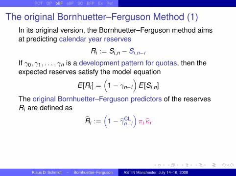
The original Bornhuetter–Ferguson Method (1)In its original version, the Bornhuetter–Ferguson method aimsat predicting calendar year reserves
Ri := Si,n − Si,n−i
If γ0, γ1, . . . , γn is a development pattern for quotas, then theexpected reserves satisfy the model equation
E [Ri ] =(
1− γn−i
)E [Si,n]
The original Bornhuetter–Ferguson predictors of the reservesRi are defined as
Ri :=(
1− γCLn−i
)πi κi
whereI γCL
n−i is the current chain–ladder quota,I πi is a volume measure, andI κi is an estimator of the expected loss ratio κi := E [Si,n/πi ]
Klaus D. Schmidt – Bornhuetter–Ferguson ASTIN Manchester, July 14–16, 2008

ROT DP oBF eBF SC BFP Ex Ref
The original Bornhuetter–Ferguson Method (1)In its original version, the Bornhuetter–Ferguson method aimsat predicting calendar year reserves
Ri := Si,n − Si,n−i
If γ0, γ1, . . . , γn is a development pattern for quotas, then theexpected reserves satisfy the model equation
E [Ri ] =(
1− γn−i
)E [Si,n]
The original Bornhuetter–Ferguson predictors of the reservesRi are defined as
Ri :=(
1− γCLn−i
)πi κi
whereI γCL
n−i is the current chain–ladder quota,I πi is a volume measure, andI κi is an estimator of the expected loss ratio κi := E [Si,n/πi ]
Klaus D. Schmidt – Bornhuetter–Ferguson ASTIN Manchester, July 14–16, 2008
ROT DP oBF eBF SC BFP Ex Ref
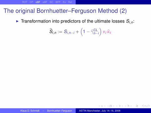
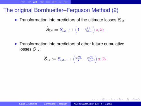
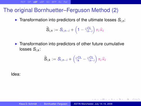
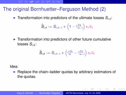
The original Bornhuetter–Ferguson Method (2)
I Transformation into predictors of the ultimate losses Si,n:
Si,n := Si,n−i +(
1− γCLn−i
)πi κi
I Transformation into predictors of other future cumulativelosses Si,k :
Si,k := Si,n−i +(γCL
k − γCLn−i
)πi κi
Idea:
I Replace the chain–ladder quotas by arbitrary estimators ofthe quotas.
I Replace the estimators πi κi by arbitrary estimators of theexpected ultimate losses E [Si,n].
Klaus D. Schmidt – Bornhuetter–Ferguson ASTIN Manchester, July 14–16, 2008
ROT DP oBF eBF SC BFP Ex Ref
The original Bornhuetter–Ferguson Method (2)
I Transformation into predictors of the ultimate losses Si,n:
Si,n := Si,n−i +(
1− γCLn−i
)πi κi
I Transformation into predictors of other future cumulativelosses Si,k :
Si,k := Si,n−i +(γCL
k − γCLn−i
)πi κi
Idea:I Replace the chain–ladder quotas by arbitrary estimators of
the quotas.I Replace the estimators πi κi by arbitrary estimators of the
expected ultimate losses E [Si,n].
Klaus D. Schmidt – Bornhuetter–Ferguson ASTIN Manchester, July 14–16, 2008

ROT DP oBF eBF SC BFP Ex Ref
Table of Contents
Run–Off Triangles of Cumulative Losses
Development Patterns
The original Bornhuetter–Ferguson Method
The extended Bornhuetter–Ferguson Method
Special CasesThe Loss–Development MethodThe Chain–Ladder MethodThe Cape Cod MethodThe Additive Method
The Bornhuetter–Ferguson Principle
An Example
References
Klaus D. Schmidt – Bornhuetter–Ferguson ASTIN Manchester, July 14–16, 2008

ROT DP oBF eBF SC BFP Ex Ref
The extended Bornhuetter–Ferguson Method (1)
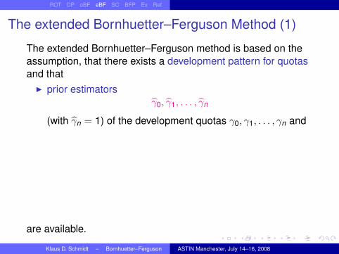
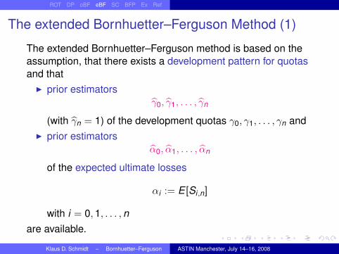
The extended Bornhuetter–Ferguson method is based on theassumption, that there exists a development pattern for quotas
and that
I prior estimatorsγ0, γ1, . . . , γn
(with γn = 1) of the development quotas γ0, γ1, . . . , γn andI prior estimators
α0, α1, . . . , αn
of the expected ultimate losses
αi := E [Si,n]
with i = 0, 1, . . . , nare available.
Klaus D. Schmidt – Bornhuetter–Ferguson ASTIN Manchester, July 14–16, 2008
ROT DP oBF eBF SC BFP Ex Ref
The extended Bornhuetter–Ferguson Method (1)
The extended Bornhuetter–Ferguson method is based on theassumption, that there exists a development pattern for quotasand that
I prior estimatorsγ0, γ1, . . . , γn
(with γn = 1) of the development quotas γ0, γ1, . . . , γn andI prior estimators
α0, α1, . . . , αn
of the expected ultimate losses
αi := E [Si,n]
with i = 0, 1, . . . , nare available.
Klaus D. Schmidt – Bornhuetter–Ferguson ASTIN Manchester, July 14–16, 2008
ROT DP oBF eBF SC BFP Ex Ref
The extended Bornhuetter–Ferguson Method (2)
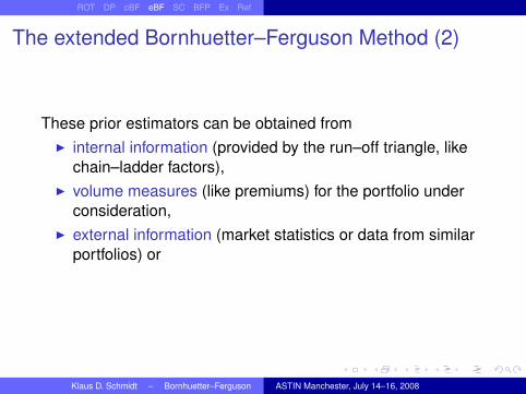
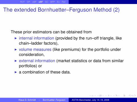
These prior estimators can be obtained fromI internal information (provided by the run–off triangle, like
chain–ladder factors),I volume measures (like premiums) for the portfolio under
consideration,I external information (market statistics or data from similar
portfolios) orI a combination of these data.
Klaus D. Schmidt – Bornhuetter–Ferguson ASTIN Manchester, July 14–16, 2008

ROT DP oBF eBF SC BFP Ex Ref
The extended Bornhuetter–Ferguson Method (2)
These prior estimators can be obtained fromI internal information (provided by the run–off triangle, like
chain–ladder factors),I volume measures (like premiums) for the portfolio under
consideration,I external information (market statistics or data from similar
portfolios) orI a combination of these data.
Klaus D. Schmidt – Bornhuetter–Ferguson ASTIN Manchester, July 14–16, 2008

ROT DP oBF eBF SC BFP Ex Ref
The extended Bornhuetter–Ferguson Method (3)
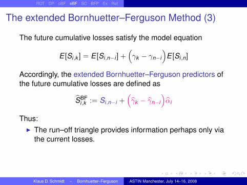
The future cumulative losses satisfy the model equation
E [Si,k ] = E [Si,n−i ] +(γk − γn−i
)E [Si,n]
Accordingly, the extended Bornhuetter–Ferguson predictors ofthe future cumulative losses are defined as
SBFi,k := Si,n−i +
(γk − γn−i
)αi
Thus:
I The run–off triangle provides information perhaps only viathe current losses.
I The predictors of the ultimate losses are obtained by linearextrapolation from the current losses.
Klaus D. Schmidt – Bornhuetter–Ferguson ASTIN Manchester, July 14–16, 2008

ROT DP oBF eBF SC BFP Ex Ref
The extended Bornhuetter–Ferguson Method (3)
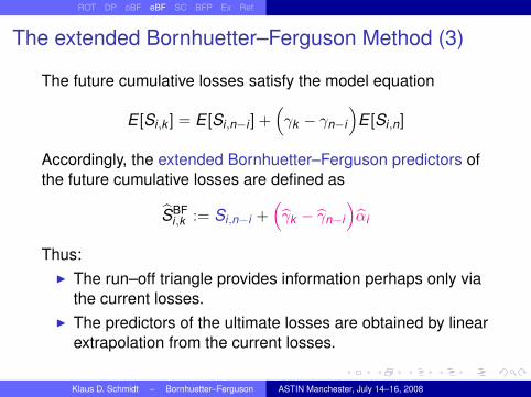
The future cumulative losses satisfy the model equation
E [Si,k ] = E [Si,n−i ] +(γk − γn−i
)E [Si,n]
Accordingly, the extended Bornhuetter–Ferguson predictors ofthe future cumulative losses are defined as
SBFi,k := Si,n−i +
(γk − γn−i
)αi
Thus:I The run–off triangle provides information perhaps only via
the current losses.I The predictors of the ultimate losses are obtained by linear
extrapolation from the current losses.
Klaus D. Schmidt – Bornhuetter–Ferguson ASTIN Manchester, July 14–16, 2008
ROT DP oBF eBF SC BFP Ex Ref
The extended Bornhuetter–Ferguson Method (3)
The future cumulative losses satisfy the model equation
E [Si,k ] = E [Si,n−i ] +(γk − γn−i
)E [Si,n]
Accordingly, the extended Bornhuetter–Ferguson predictors ofthe future cumulative losses are defined as
SBFi,k := Si,n−i +
(γk − γn−i
)αi
Thus:I The run–off triangle provides information perhaps only via
the current losses.I The predictors of the ultimate losses are obtained by linear
extrapolation from the current losses.
Klaus D. Schmidt – Bornhuetter–Ferguson ASTIN Manchester, July 14–16, 2008

ROT DP oBF eBF SC BFP Ex Ref
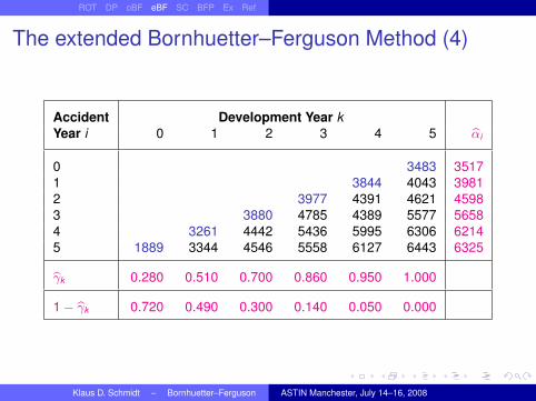
The extended Bornhuetter–Ferguson Method (4)
Accident Development Year kYear i 0 1 2 3 4 5 bαi
0 3483 35171 3844
4043
39812 3977
4391 4621
45983 3880
4785 4389 5577
56584 3261
4442 5436 5995 6306
62145 1889
3344 4546 5558 6127 6443
6325
bγk 0.280 0.510 0.700 0.860 0.950 1.000
1− bγk 0.720 0.490 0.300 0.140 0.050 0.000
Klaus D. Schmidt – Bornhuetter–Ferguson ASTIN Manchester, July 14–16, 2008
ROT DP oBF eBF SC BFP Ex Ref
The extended Bornhuetter–Ferguson Method (4)
Accident Development Year kYear i 0 1 2 3 4 5 bαi
0 3483 35171 3844 4043 39812 3977 4391 4621 45983 3880 4785 4389 5577 56584 3261 4442 5436 5995 6306 62145 1889 3344 4546 5558 6127 6443 6325
bγk 0.280 0.510 0.700 0.860 0.950 1.000
1− bγk 0.720 0.490 0.300 0.140 0.050 0.000
Klaus D. Schmidt – Bornhuetter–Ferguson ASTIN Manchester, July 14–16, 2008

ROT DP oBF eBF SC BFP Ex Ref LD CL CC AD
Table of Contents
Run–Off Triangles of Cumulative Losses
Development Patterns
The original Bornhuetter–Ferguson Method
The extended Bornhuetter–Ferguson Method
Special CasesThe Loss–Development MethodThe Chain–Ladder MethodThe Cape Cod MethodThe Additive Method
The Bornhuetter–Ferguson Principle
An Example
References
Klaus D. Schmidt – Bornhuetter–Ferguson ASTIN Manchester, July 14–16, 2008
ROT DP oBF eBF SC BFP Ex Ref LD CL CC AD
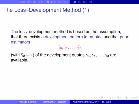
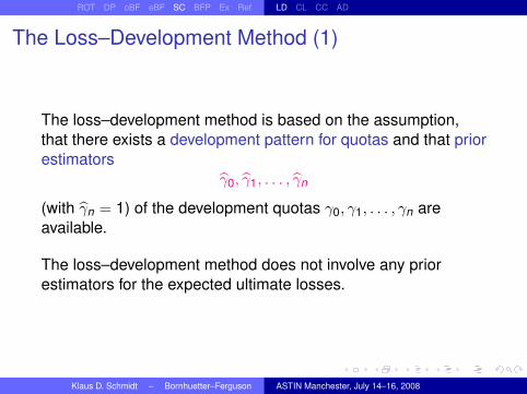
The Loss–Development Method (1)
The loss–development method is based on the assumption,that there exists a development pattern for quotas and that priorestimators
γ0, γ1, . . . , γn
(with γn = 1) of the development quotas γ0, γ1, . . . , γn areavailable.
The loss–development method does not involve any priorestimators for the expected ultimate losses.
Klaus D. Schmidt – Bornhuetter–Ferguson ASTIN Manchester, July 14–16, 2008
ROT DP oBF eBF SC BFP Ex Ref LD CL CC AD
The Loss–Development Method (1)
The loss–development method is based on the assumption,that there exists a development pattern for quotas and that priorestimators
γ0, γ1, . . . , γn
(with γn = 1) of the development quotas γ0, γ1, . . . , γn areavailable.
The loss–development method does not involve any priorestimators for the expected ultimate losses.
Klaus D. Schmidt – Bornhuetter–Ferguson ASTIN Manchester, July 14–16, 2008

ROT DP oBF eBF SC BFP Ex Ref LD CL CC AD
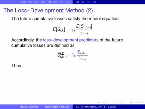
The Loss–Development Method (2)The future cumulative losses satisfy the model equation
E [Si,k ] = γkE [Si,n−i ]
γn−i
Accordingly, the loss–development predictors of the futurecumulative losses are defined as
SLDi,k := γk
Si,n−i
γn−i
Thus:
I The run–off triangle provides information perhaps only viathe current losses.
I The predictors of the ultimate losses are obtained byscaling the current losses.
I The predictors of other future cumulative losses areobtained by scaling the predictors of the ultimate losses.Klaus D. Schmidt – Bornhuetter–Ferguson ASTIN Manchester, July 14–16, 2008

ROT DP oBF eBF SC BFP Ex Ref LD CL CC AD
The Loss–Development Method (2)The future cumulative losses satisfy the model equation
E [Si,k ] = γkE [Si,n−i ]
γn−i
Accordingly, the loss–development predictors of the futurecumulative losses are defined as
SLDi,k := γk
Si,n−i
γn−i
Thus:
I The run–off triangle provides information perhaps only viathe current losses.
I The predictors of the ultimate losses are obtained byscaling the current losses.
I The predictors of other future cumulative losses areobtained by scaling the predictors of the ultimate losses.Klaus D. Schmidt – Bornhuetter–Ferguson ASTIN Manchester, July 14–16, 2008
ROT DP oBF eBF SC BFP Ex Ref LD CL CC AD
The Loss–Development Method (2)The future cumulative losses satisfy the model equation
E [Si,k ] = γkE [Si,n−i ]
γn−i
Accordingly, the loss–development predictors of the futurecumulative losses are defined as
SLDi,k := γk
Si,n−i
γn−i
Thus:I The run–off triangle provides information perhaps only via
the current losses.I The predictors of the ultimate losses are obtained by
scaling the current losses.I The predictors of other future cumulative losses are
obtained by scaling the predictors of the ultimate losses.Klaus D. Schmidt – Bornhuetter–Ferguson ASTIN Manchester, July 14–16, 2008
ROT DP oBF eBF SC BFP Ex Ref LD CL CC AD
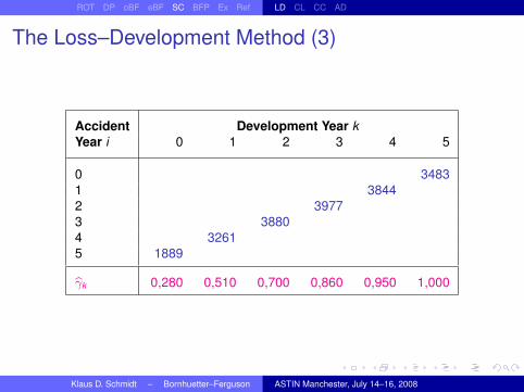
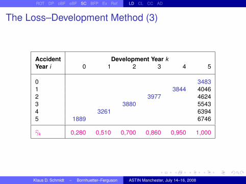
The Loss–Development Method (3)
Accident Development Year kYear i 0 1 2 3 4 5
0 34831 3844
4046
2 3977
4393 4624
3 3880
4767 5266 5543
4 3261
4476 5499 6074 6394
5 1889
3440 4722 5802 6409 6746
bγk 0,280 0,510 0,700 0,860 0,950 1,000
Klaus D. Schmidt – Bornhuetter–Ferguson ASTIN Manchester, July 14–16, 2008
ROT DP oBF eBF SC BFP Ex Ref LD CL CC AD
The Loss–Development Method (3)
Accident Development Year kYear i 0 1 2 3 4 5
0 34831 3844 40462 3977
4393
46243 3880
4767 5266
55434 3261
4476 5499 6074
63945 1889
3440 4722 5802 6409
6746
bγk 0,280 0,510 0,700 0,860 0,950 1,000
Klaus D. Schmidt – Bornhuetter–Ferguson ASTIN Manchester, July 14–16, 2008
ROT DP oBF eBF SC BFP Ex Ref LD CL CC AD
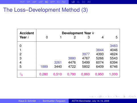
The Loss–Development Method (3)
Accident Development Year kYear i 0 1 2 3 4 5
0 34831 3844 40462 3977 4393 46243 3880 4767 5266 55434 3261 4476 5499 6074 63945 1889 3440 4722 5802 6409 6746
bγk 0,280 0,510 0,700 0,860 0,950 1,000
Klaus D. Schmidt – Bornhuetter–Ferguson ASTIN Manchester, July 14–16, 2008
ROT DP oBF eBF SC BFP Ex Ref LD CL CC AD
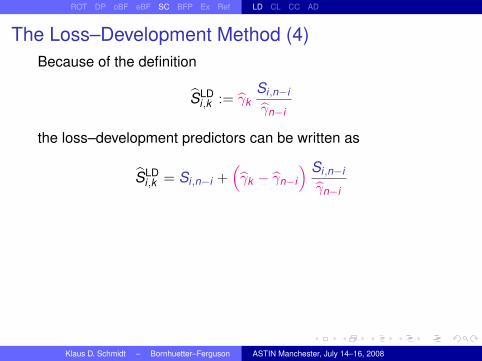
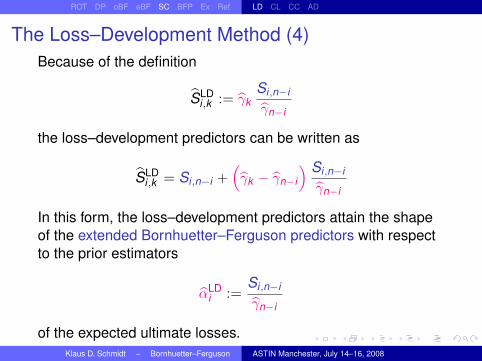
The Loss–Development Method (4)Because of the definition
SLDi,k := γk
Si,n−i
γn−i
the loss–development predictors can be written as
SLDi,k = Si,n−i +
(γk − γn−i
) Si,n−i
γn−i
In this form, the loss–development predictors attain the shapeof the extended Bornhuetter–Ferguson predictors with respectto the prior estimators
αLDi :=
Si,n−i
γn−i
of the expected ultimate losses.
Klaus D. Schmidt – Bornhuetter–Ferguson ASTIN Manchester, July 14–16, 2008
ROT DP oBF eBF SC BFP Ex Ref LD CL CC AD
The Loss–Development Method (4)Because of the definition
SLDi,k := γk
Si,n−i
γn−i
the loss–development predictors can be written as
SLDi,k = Si,n−i +
(γk − γn−i
) Si,n−i
γn−i
In this form, the loss–development predictors attain the shapeof the extended Bornhuetter–Ferguson predictors with respectto the prior estimators
αLDi :=
Si,n−i
γn−i
of the expected ultimate losses.Klaus D. Schmidt – Bornhuetter–Ferguson ASTIN Manchester, July 14–16, 2008

ROT DP oBF eBF SC BFP Ex Ref LD CL CC AD
Table of Contents
Run–Off Triangles of Cumulative Losses
Development Patterns
The original Bornhuetter–Ferguson Method
The extended Bornhuetter–Ferguson Method
Special CasesThe Loss–Development MethodThe Chain–Ladder MethodThe Cape Cod MethodThe Additive Method
The Bornhuetter–Ferguson Principle
An Example
References
Klaus D. Schmidt – Bornhuetter–Ferguson ASTIN Manchester, July 14–16, 2008

ROT DP oBF eBF SC BFP Ex Ref LD CL CC AD
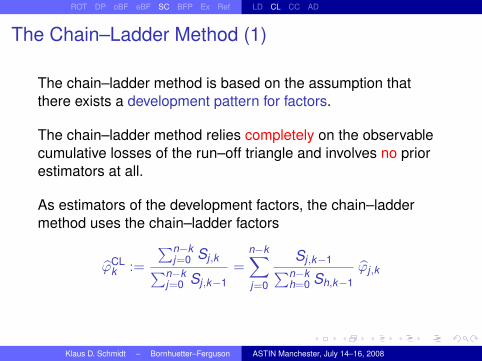
The Chain–Ladder Method (1)
The chain–ladder method is based on the assumption thatthere exists a development pattern for factors.
The chain–ladder method relies completely on the observablecumulative losses of the run–off triangle and involves no priorestimators at all.
As estimators of the development factors, the chain–laddermethod uses the chain–ladder factors
ϕCLk :=
∑n−kj=0 Sj,k∑n−k
j=0 Sj,k−1=
n−k∑j=0
Sj,k−1∑n−kh=0 Sh,k−1
ϕj,k
Klaus D. Schmidt – Bornhuetter–Ferguson ASTIN Manchester, July 14–16, 2008

ROT DP oBF eBF SC BFP Ex Ref LD CL CC AD
The Chain–Ladder Method (1)
The chain–ladder method is based on the assumption thatthere exists a development pattern for factors.
The chain–ladder method relies completely on the observablecumulative losses of the run–off triangle and involves no priorestimators at all.
As estimators of the development factors, the chain–laddermethod uses the chain–ladder factors
ϕCLk :=
∑n−kj=0 Sj,k∑n−k
j=0 Sj,k−1=
n−k∑j=0
Sj,k−1∑n−kh=0 Sh,k−1
ϕj,k
Klaus D. Schmidt – Bornhuetter–Ferguson ASTIN Manchester, July 14–16, 2008

ROT DP oBF eBF SC BFP Ex Ref LD CL CC AD
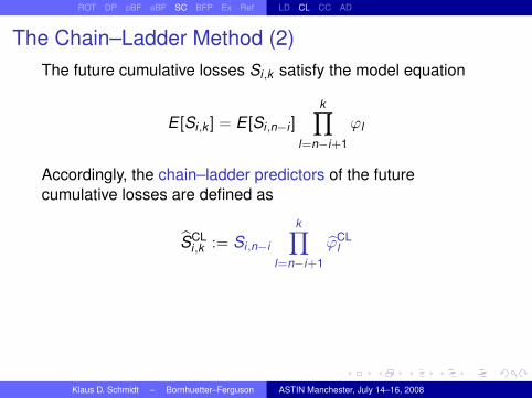
The Chain–Ladder Method (2)The future cumulative losses Si,k satisfy the model equation
E [Si,k ] = E [Si,n−i ]k∏
l=n−i+1
ϕl
Accordingly, the chain–ladder predictors of the futurecumulative losses are defined as
SCLi,k := Si,n−i
k∏l=n−i+1
ϕCLl
Thus:
I The chain–ladder method consists in successive scaling ofthe current loss Si,n−i to the level of the future cumulativeloss Si,k .
Klaus D. Schmidt – Bornhuetter–Ferguson ASTIN Manchester, July 14–16, 2008
ROT DP oBF eBF SC BFP Ex Ref LD CL CC AD
The Chain–Ladder Method (2)The future cumulative losses Si,k satisfy the model equation
E [Si,k ] = E [Si,n−i ]k∏
l=n−i+1
ϕl
Accordingly, the chain–ladder predictors of the futurecumulative losses are defined as
SCLi,k := Si,n−i
k∏l=n−i+1
ϕCLl
Thus:
I The chain–ladder method consists in successive scaling ofthe current loss Si,n−i to the level of the future cumulativeloss Si,k .
Klaus D. Schmidt – Bornhuetter–Ferguson ASTIN Manchester, July 14–16, 2008

ROT DP oBF eBF SC BFP Ex Ref LD CL CC AD
The Chain–Ladder Method (2)The future cumulative losses Si,k satisfy the model equation
E [Si,k ] = E [Si,n−i ]k∏
l=n−i+1
ϕl
Accordingly, the chain–ladder predictors of the futurecumulative losses are defined as
SCLi,k := Si,n−i
k∏l=n−i+1
ϕCLl
Thus:I The chain–ladder method consists in successive scaling of
the current loss Si,n−i to the level of the future cumulativeloss Si,k .
Klaus D. Schmidt – Bornhuetter–Ferguson ASTIN Manchester, July 14–16, 2008

ROT DP oBF eBF SC BFP Ex Ref LD CL CC AD
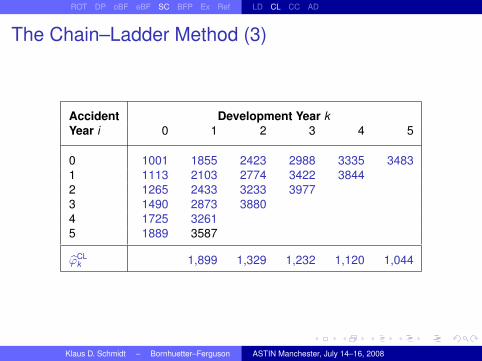
The Chain–Ladder Method (3)
Accident Development Year kYear i 0 1 2 3 4 5
0 1001 1855 2423 2988 3335 34831 1113 2103 2774 3422 3844
4013
2 1265 2433 3233 3977
4454 4650
3 1490 2873 3880
4780 5354 5590
4 1725 3261
4334 5339 5980 6243
5 1889
3587 4767 5873 6578 6867
bϕCLk 1,899 1,329 1,232 1,120 1,044
Klaus D. Schmidt – Bornhuetter–Ferguson ASTIN Manchester, July 14–16, 2008
ROT DP oBF eBF SC BFP Ex Ref LD CL CC AD
The Chain–Ladder Method (3)
Accident Development Year kYear i 0 1 2 3 4 5
0 1001 1855 2423 2988 3335 34831 1113 2103 2774 3422 3844
4013
2 1265 2433 3233 3977
4454 4650
3 1490 2873 3880
4780 5354 5590
4 1725 3261
4334 5339 5980 6243
5 1889 3587
4767 5873 6578 6867
bϕCLk 1,899 1,329 1,232 1,120 1,044
Klaus D. Schmidt – Bornhuetter–Ferguson ASTIN Manchester, July 14–16, 2008

ROT DP oBF eBF SC BFP Ex Ref LD CL CC AD
The Chain–Ladder Method (3)
Accident Development Year kYear i 0 1 2 3 4 5
0 1001 1855 2423 2988 3335 34831 1113 2103 2774 3422 3844
4013
2 1265 2433 3233 3977
4454 4650
3 1490 2873 3880
4780 5354 5590
4 1725 3261 4334
5339 5980 6243
5 1889 3587 4767
5873 6578 6867
bϕCLk 1,899 1,329 1,232 1,120 1,044
Klaus D. Schmidt – Bornhuetter–Ferguson ASTIN Manchester, July 14–16, 2008

ROT DP oBF eBF SC BFP Ex Ref LD CL CC AD
The Chain–Ladder Method (3)
Accident Development Year kYear i 0 1 2 3 4 5
0 1001 1855 2423 2988 3335 34831 1113 2103 2774 3422 3844
4013
2 1265 2433 3233 3977
4454 4650
3 1490 2873 3880 4780
5354 5590
4 1725 3261 4334 5339
5980 6243
5 1889 3587 4767 5873
6578 6867
bϕCLk 1,899 1,329 1,232 1,120 1,044
Klaus D. Schmidt – Bornhuetter–Ferguson ASTIN Manchester, July 14–16, 2008

ROT DP oBF eBF SC BFP Ex Ref LD CL CC AD
The Chain–Ladder Method (3)
Accident Development Year kYear i 0 1 2 3 4 5
0 1001 1855 2423 2988 3335 34831 1113 2103 2774 3422 3844
4013
2 1265 2433 3233 3977 4454
4650
3 1490 2873 3880 4780 5354
5590
4 1725 3261 4334 5339 5980
6243
5 1889 3587 4767 5873 6578
6867
bϕCLk 1,899 1,329 1,232 1,120 1,044
Klaus D. Schmidt – Bornhuetter–Ferguson ASTIN Manchester, July 14–16, 2008
ROT DP oBF eBF SC BFP Ex Ref LD CL CC AD
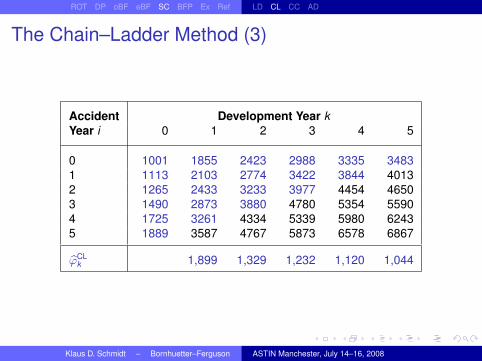
The Chain–Ladder Method (3)
Accident Development Year kYear i 0 1 2 3 4 5
0 1001 1855 2423 2988 3335 34831 1113 2103 2774 3422 3844 40132 1265 2433 3233 3977 4454 46503 1490 2873 3880 4780 5354 55904 1725 3261 4334 5339 5980 62435 1889 3587 4767 5873 6578 6867
bϕCLk 1,899 1,329 1,232 1,120 1,044
Klaus D. Schmidt – Bornhuetter–Ferguson ASTIN Manchester, July 14–16, 2008
ROT DP oBF eBF SC BFP Ex Ref LD CL CC AD
The Chain–Ladder Method (4)
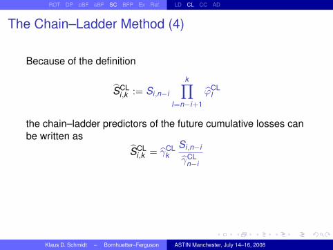
Because of the definition
SCLi,k := Si,n−i
k∏l=n−i+1
ϕCLl
the chain–ladder predictors of the future cumulative losses canbe written as
SCLi,k = γCL
kSi,n−i
γCLn−i
In this form, the chain–ladder predictors attain the shape of theloss–development predictors with respect to the chain–ladderquotas.
Klaus D. Schmidt – Bornhuetter–Ferguson ASTIN Manchester, July 14–16, 2008

ROT DP oBF eBF SC BFP Ex Ref LD CL CC AD
The Chain–Ladder Method (4)
Because of the definition
SCLi,k := Si,n−i
k∏l=n−i+1
ϕCLl
the chain–ladder predictors of the future cumulative losses canbe written as
SCLi,k = γCL
kSi,n−i
γCLn−i
In this form, the chain–ladder predictors attain the shape of theloss–development predictors with respect to the chain–ladderquotas.
Klaus D. Schmidt – Bornhuetter–Ferguson ASTIN Manchester, July 14–16, 2008
ROT DP oBF eBF SC BFP Ex Ref LD CL CC AD
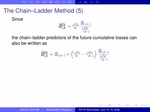
The Chain–Ladder Method (5)Since
SCLi,k = γCL
kSi,n−i
γCLn−i
the chain–ladder predictors of the future cumulative losses canalso be written as
SCLi,k = Si,n−i +
(γCL
k − γCLn−i
) Si,n−i
γCLn−i
In this form, the chain–ladder predictors attain the shape of theextended Bornhuetter–Ferguson predictors with respect to thechain–ladder quotas and the prior estimators
αCLi :=
Si,n−i
γCLn−i
of the expected ultimate losses.
Klaus D. Schmidt – Bornhuetter–Ferguson ASTIN Manchester, July 14–16, 2008
ROT DP oBF eBF SC BFP Ex Ref LD CL CC AD
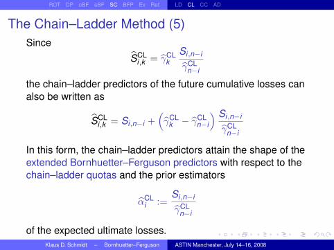
The Chain–Ladder Method (5)Since
SCLi,k = γCL
kSi,n−i
γCLn−i
the chain–ladder predictors of the future cumulative losses canalso be written as
SCLi,k = Si,n−i +
(γCL
k − γCLn−i
) Si,n−i
γCLn−i
In this form, the chain–ladder predictors attain the shape of theextended Bornhuetter–Ferguson predictors with respect to thechain–ladder quotas and the prior estimators
αCLi :=
Si,n−i
γCLn−i
of the expected ultimate losses.Klaus D. Schmidt – Bornhuetter–Ferguson ASTIN Manchester, July 14–16, 2008

ROT DP oBF eBF SC BFP Ex Ref LD CL CC AD
Table of Contents
Run–Off Triangles of Cumulative Losses
Development Patterns
The original Bornhuetter–Ferguson Method
The extended Bornhuetter–Ferguson Method
Special CasesThe Loss–Development MethodThe Chain–Ladder MethodThe Cape Cod MethodThe Additive Method
The Bornhuetter–Ferguson Principle
An Example
References
Klaus D. Schmidt – Bornhuetter–Ferguson ASTIN Manchester, July 14–16, 2008
ROT DP oBF eBF SC BFP Ex Ref LD CL CC AD
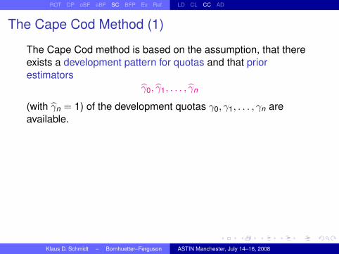
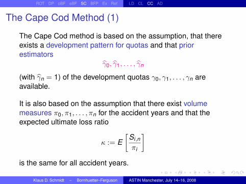
The Cape Cod Method (1)
The Cape Cod method is based on the assumption, that thereexists a development pattern for quotas and that priorestimators
γ0, γ1, . . . , γn
(with γn = 1) of the development quotas γ0, γ1, . . . , γn areavailable.
It is also based on the assumption that there exist volumemeasures π0, π1, . . . , πn for the accident years and that theexpected ultimate loss ratio
κ := E[
Si,n
πi
]is the same for all accident years.
Klaus D. Schmidt – Bornhuetter–Ferguson ASTIN Manchester, July 14–16, 2008
ROT DP oBF eBF SC BFP Ex Ref LD CL CC AD
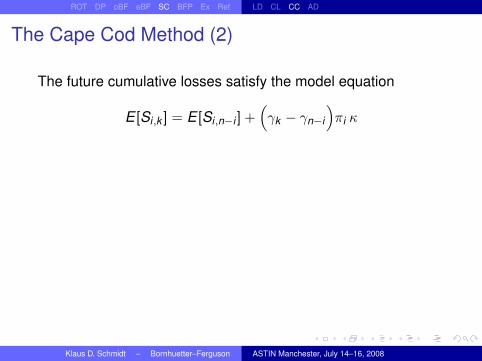
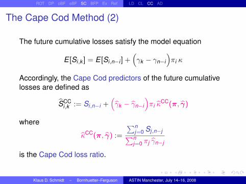
The Cape Cod Method (2)
The future cumulative losses satisfy the model equation
E [Si,k ] = E [Si,n−i ] +(γk − γn−i
)πi κ
Accordingly, the Cape Cod predictors of the future cumulativelosses are defined as
SCCi,k := Si,n−i +
(γk − γn−i
)πi κ
CC(π, γ)
where
κCC(π, γ) :=
∑nj=0 Sj,n−j∑n
j=0 πj γn−j
is the Cape Cod loss ratio.
Klaus D. Schmidt – Bornhuetter–Ferguson ASTIN Manchester, July 14–16, 2008

ROT DP oBF eBF SC BFP Ex Ref LD CL CC AD
The Cape Cod Method (2)
The future cumulative losses satisfy the model equation
E [Si,k ] = E [Si,n−i ] +(γk − γn−i
)πi κ
Accordingly, the Cape Cod predictors of the future cumulativelosses are defined as
SCCi,k := Si,n−i +
(γk − γn−i
)πi κ
CC(π, γ)
where
κCC(π, γ) :=
∑nj=0 Sj,n−j∑n
j=0 πj γn−j
is the Cape Cod loss ratio.
Klaus D. Schmidt – Bornhuetter–Ferguson ASTIN Manchester, July 14–16, 2008

ROT DP oBF eBF SC BFP Ex Ref LD CL CC AD
The Cape Cod Method (3)
Therefore, the Cape Cod predictors of the future cumulativelosses have the shape of the extended Bornhuetter–Fergusonpredictors with respect to the Cape Cod estimators
αCCi := πi κ
CC(π, γ)
of the expected ultimate losses.
Klaus D. Schmidt – Bornhuetter–Ferguson ASTIN Manchester, July 14–16, 2008

ROT DP oBF eBF SC BFP Ex Ref LD CL CC AD
Table of Contents
Run–Off Triangles of Cumulative Losses
Development Patterns
The original Bornhuetter–Ferguson Method
The extended Bornhuetter–Ferguson Method
Special CasesThe Loss–Development MethodThe Chain–Ladder MethodThe Cape Cod MethodThe Additive Method
The Bornhuetter–Ferguson Principle
An Example
References
Klaus D. Schmidt – Bornhuetter–Ferguson ASTIN Manchester, July 14–16, 2008

ROT DP oBF eBF SC BFP Ex Ref LD CL CC AD
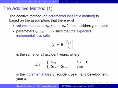
The Additive Method (1)
The additive method (or incremental loss ratio method) isbased on the assumption, that there exist
I volume measures π0, π1, . . . , πn for the accident years, andI parameters ζ0, ζ1, . . . , ζn such that the expected
incremental loss ratio
ζk := E[
Zi,k
πi
]is the same for all accident years, where
Zi,k :=
{Si,0 if k = 0Si,k − Si,k−1 else
is the incremental loss of accident year i and developmentyear k .
Klaus D. Schmidt – Bornhuetter–Ferguson ASTIN Manchester, July 14–16, 2008

ROT DP oBF eBF SC BFP Ex Ref LD CL CC AD
The Additive Method (1)
The additive method (or incremental loss ratio method) isbased on the assumption, that there exist
I volume measures π0, π1, . . . , πn for the accident years, andI parameters ζ0, ζ1, . . . , ζn such that the expected
incremental loss ratio
ζk := E[
Zi,k
πi
]is the same for all accident years, where
Zi,k :=
{Si,0 if k = 0Si,k − Si,k−1 else
is the incremental loss of accident year i and developmentyear k .
Klaus D. Schmidt – Bornhuetter–Ferguson ASTIN Manchester, July 14–16, 2008

ROT DP oBF eBF SC BFP Ex Ref LD CL CC AD
The Additive Method (2)The cumulative and incremental losses satisfy the modelequation
E [Si,k ] = E [Si,n−i ] + πi
k∑l=n−i+1
ζl
Accordingly, the additive predictors of the future cumulativelosses are defined as
SADi,k := Si,n−i + πi
k∑l=n−i+1
ζADl
where
ζADk :=
∑n−kj=0 Zj,k∑n−kj=0 πj
is the additive incremental loss ratio of development year k .
Klaus D. Schmidt – Bornhuetter–Ferguson ASTIN Manchester, July 14–16, 2008

ROT DP oBF eBF SC BFP Ex Ref LD CL CC AD
The Additive Method (2)The cumulative and incremental losses satisfy the modelequation
E [Si,k ] = E [Si,n−i ] + πi
k∑l=n−i+1
ζl
Accordingly, the additive predictors of the future cumulativelosses are defined as
SADi,k := Si,n−i + πi
k∑l=n−i+1
ζADl
where
ζADk :=
∑n−kj=0 Zj,k∑n−kj=0 πj
is the additive incremental loss ratio of development year k .Klaus D. Schmidt – Bornhuetter–Ferguson ASTIN Manchester, July 14–16, 2008

ROT DP oBF eBF SC BFP Ex Ref LD CL CC AD
The Additive Method (3)
Since
SADi,k := Si,n−i + πi
k∑l=n−i+1
ζADl
the additive predictors can be written as
SADi,k := Si,n−i +
(∑kl=0 ζAD
l∑nl=0 ζAD
l
−∑n−i
l=0 ζADl∑n
l=0 ζADl
)(πi
n∑l=0
ζADl
)
or asSAD
i,k := Si,n−i +(γAD
k (π)− γADn−i(π)
)αAD
i (π)
In this form, the additive predictors of the future cumulativelosses have the shape of the extended Bornhuetter–Fergusonpredictors with respect to the additive quotas γAD
k (π) and theadditive estimators αAD
i (π) of the expected ultimate losses.
Klaus D. Schmidt – Bornhuetter–Ferguson ASTIN Manchester, July 14–16, 2008

ROT DP oBF eBF SC BFP Ex Ref LD CL CC AD
The Additive Method (3)
Since
SADi,k := Si,n−i + πi
k∑l=n−i+1
ζADl
the additive predictors can be written as
SADi,k := Si,n−i +
(∑kl=0 ζAD
l∑nl=0 ζAD
l
−∑n−i
l=0 ζADl∑n
l=0 ζADl
)(πi
n∑l=0
ζADl
)
or asSAD
i,k := Si,n−i +(γAD
k (π)− γADn−i(π)
)αAD
i (π)
In this form, the additive predictors of the future cumulativelosses have the shape of the extended Bornhuetter–Fergusonpredictors with respect to the additive quotas γAD
k (π) and theadditive estimators αAD
i (π) of the expected ultimate losses.
Klaus D. Schmidt – Bornhuetter–Ferguson ASTIN Manchester, July 14–16, 2008
ROT DP oBF eBF SC BFP Ex Ref LD CL CC AD
The Additive Method (4)
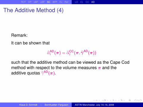
Remark:
It can be shown that
αADi (π) = αCC
i (π, γAD(π))
such that the additive method can be viewed as the Cape Codmethod with respect to the volume measures π and theadditive quotas γAD(π).
Klaus D. Schmidt – Bornhuetter–Ferguson ASTIN Manchester, July 14–16, 2008

ROT DP oBF eBF SC BFP Ex Ref
Table of Contents
Run–Off Triangles of Cumulative Losses
Development Patterns
The original Bornhuetter–Ferguson Method
The extended Bornhuetter–Ferguson Method
Special CasesThe Loss–Development MethodThe Chain–Ladder MethodThe Cape Cod MethodThe Additive Method
The Bornhuetter–Ferguson Principle
An Example
References
Klaus D. Schmidt – Bornhuetter–Ferguson ASTIN Manchester, July 14–16, 2008

ROT DP oBF eBF SC BFP Ex Ref
The Bornhuetter–Ferguson Principle (1)
Comparison of certain versions of the extendedBornhuetter–Ferguson method:
Prior Estimators Prior Estimators of Cumulative Quotasof ExpectedUltimate Losses γexternal γCL γAD(π)
αexternal Bornhuetter–FergusonMethod (external)
αLD(γ) Loss–Development Chain–LadderMethod (external) Method
αCC(π, γ) Cape Cod AdditiveMethod (external) Method
Klaus D. Schmidt – Bornhuetter–Ferguson ASTIN Manchester, July 14–16, 2008

ROT DP oBF eBF SC BFP Ex Ref
The Bornhuetter–Ferguson Principle (2)
The Bornhuetter–Ferguson principle consists ofI an analytic part,
in which known methods of loss reserving are interpretedas versions of the extended Bornhuetter–Fergusonmethod,
I a synthetic part,in which components of different versions of the extendedBornhuetter–Ferguson method are used to construct newversions of the extended Bornhuetter–Ferguson method,and
I the simultaneous application of several versions of theextended Bornhuetter–Ferguson method to a given run–offtriangle of cumulative losses.
Klaus D. Schmidt – Bornhuetter–Ferguson ASTIN Manchester, July 14–16, 2008

ROT DP oBF eBF SC BFP Ex Ref
The Bornhuetter–Ferguson Principle (3)
Application of the Bornhuetter–Ferguson principle may result inI the selection of reliable predictors,I the selection of reliable ranges,I the comparison of the given portfolio with a market
portfolio, andI the control of pricing.
In either case, careful actuarial judgement of the quality of thesources of information underlying the different versions of theextended Bornhuetter–Ferguson method is essential.
Klaus D. Schmidt – Bornhuetter–Ferguson ASTIN Manchester, July 14–16, 2008

ROT DP oBF eBF SC BFP Ex Ref
Table of Contents
Run–Off Triangles of Cumulative Losses
Development Patterns
The original Bornhuetter–Ferguson Method
The extended Bornhuetter–Ferguson Method
Special CasesThe Loss–Development MethodThe Chain–Ladder MethodThe Cape Cod MethodThe Additive Method
The Bornhuetter–Ferguson Principle
An Example
References
Klaus D. Schmidt – Bornhuetter–Ferguson ASTIN Manchester, July 14–16, 2008

ROT DP oBF eBF SC BFP Ex Ref
An Example
Modified example:
Acc. Development Year kYear i 0 1 2 3 4 5 πi bαext
i
0 1001 1855 2423 2988 3335 3483 4000 35201 1113 2103 2774 3422 3844 4500 39802 1265 2433 3233 3977 5300 46203 1490 2873 3880 6000 56604 1725 4261 6900 62105 1889 8200 6330
bγextk 0.2800 0.5300 0.7100 0.8600 0.9500 1.0000
Klaus D. Schmidt – Bornhuetter–Ferguson ASTIN Manchester, July 14–16, 2008
ROT DP oBF eBF SC BFP Ex Ref
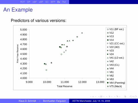
An Example
Predictors of various versions:
4.000
4.100
4.200
4.300
4.400
4.500
4.600
4.700
4.800
4.900
5.000
9.000 10.000 11.000 12.000 13.000
Total Reserve
Firs
t-Y
ear
Res
erve
V11 (BF ext.)V12V13V14V21 (CC ext.)V22 (AD)V23V24V41 (LD ext.)V42V43 (CL)V44V61V62V63V64 (Panning)V75 (Mack)
Klaus D. Schmidt – Bornhuetter–Ferguson ASTIN Manchester, July 14–16, 2008

ROT DP oBF eBF SC BFP Ex Ref
An Example
Reliable predictors:
4.000
4.100
4.200
4.300
4.400
4.500
4.600
4.700
4.800
4.900
5.000
9.000 10.000 11.000 12.000 13.000
Total Reserve
Firs
t-Y
ear
Res
erve
V22 (AD)
V23
V24
V42
V44
V62
V63
V64 (Panning)
Klaus D. Schmidt – Bornhuetter–Ferguson ASTIN Manchester, July 14–16, 2008

ROT DP oBF eBF SC BFP Ex Ref
An Example
Selected predictor:
4.000
4.100
4.200
4.300
4.400
4.500
4.600
4.700
4.800
4.900
5.000
9.000 10.000 11.000 12.000 13.000
Total Reserve
Firs
t-Y
ear
Res
erve
V23 V42
Klaus D. Schmidt – Bornhuetter–Ferguson ASTIN Manchester, July 14–16, 2008

ROT DP oBF eBF SC BFP Ex Ref
Table of Contents
Run–Off Triangles of Cumulative Losses
Development Patterns
The original Bornhuetter–Ferguson Method
The extended Bornhuetter–Ferguson Method
Special CasesThe Loss–Development MethodThe Chain–Ladder MethodThe Cape Cod MethodThe Additive Method
The Bornhuetter–Ferguson Principle
An Example
References
Klaus D. Schmidt – Bornhuetter–Ferguson ASTIN Manchester, July 14–16, 2008

ROT DP oBF eBF SC BFP Ex Ref
ReferencesI P. Paczkowski, K.D. Schmidt and M. Zocher [2007]:
Dresden Loss Reserving Tool.http://www.math.tu-dresden.de/sto/schmidt/lossreserving/
I M. Radtke and K.D. Schmidt [2004]:Handbuch zur Schadenreservierung.Karlsruhe: Verlag Versicherungswirtschaft.
I K.D. Schmidt [permanent update]:A Bibliography of Loss Reserving.http://www.math.tu-dresden.de/sto/schmidt/dsvm/reserve.pdf
I K.D. Schmidt [2006]:Methods and Models of Loss Reserving Based on Run–OffTriangles: A Unifying Survey. CAS Forum Fall 2006.
I K.D. Schmidt and M. Zocher [2008]:The Bornhuetter–Ferguson Principle. Variance (in press).
Klaus D. Schmidt – Bornhuetter–Ferguson ASTIN Manchester, July 14–16, 2008