RUHRECONOMIC PAPERS

Border Eff ects in House Prices

#511

Martin MicheliJan Rouwendal Jasper Dekkers

Imprint

Ruhr Economic Papers

Published by

Ruhr-Universität Bochum (RUB), Department of EconomicsUniversitätsstr. 150, 44801 Bochum, Germany

Technische Universität Dortmund, Department of Economic and Social SciencesVogelpothsweg 87, 44227 Dortmund, Germany

Universität Duisburg-Essen, Department of EconomicsUniversitätsstr. 12, 45117 Essen, Germany

Rheinisch-Westfälisches Institut für Wirtschaftsforschung (RWI)Hohenzollernstr. 1-3, 45128 Essen, Germany

Editors

Prof. Dr. Thomas K. BauerRUB, Department of Economics, Empirical EconomicsPhone: +49 (0) 234/3 22 83 41, e-mail: thomas.bauer@rub.de

Prof. Dr. Wolfgang LeiningerTechnische Universität Dortmund, Department of Economic and Social SciencesEconomics – MicroeconomicsPhone: +49 (0) 231/7 55-3297, e-mail: W.Leininger@wiso.uni-dortmund.de

Prof. Dr. Volker ClausenUniversity of Duisburg-Essen, Department of EconomicsInternational EconomicsPhone: +49 (0) 201/1 83-3655, e-mail: vclausen@vwl.uni-due.de

Prof. Dr. Roland Döhrn, Prof. Dr. Manuel Frondel, Prof. Dr. Jochen KluveRWI, Phone: +49 (0) 201/81 49-213, e-mail: presse@rwi-essen.de

Editorial Offi ce

Sabine WeilerRWI, Phone: +49 (0) 201/81 49-213, e-mail: sabine.weiler@rwi-essen.de

Ruhr Economic Papers #511

Responsible Editor: Roland Döhrn

All rights reserved. Bochum, Dortmund, Duisburg, Essen, Germany, 2014

ISSN 1864-4872 (online) – ISBN 978-3-86788-586-7The working papers published in the Series constitute work in progress circulated to stimulate discussion and critical comments. Views expressed represent exclusively the authors’ own opinions and do not necessarily refl ect those of the editors.

Ruhr Economic Papers #511

Martin Micheli, Jan Rouwendal, and Jasper Dekkers

Border Eff ects in House Prices

Bibliografi sche Informationen der Deutschen Nationalbibliothek

Die Deutsche Bibliothek verzeichnet diese Publikation in der deutschen National-bibliografi e; detaillierte bibliografi sche Daten sind im Internet über: http://dnb.d-nb.de abrufb ar.

http://dx.doi.org/10.4419/86788586ISSN 1864-4872 (online)ISBN 978-3-86788-586-7

Martin Micheli, Jan Rouwendal, and Jasper Dekkers1

Border Eff ects in House Prices

Abstract

We estimate the eff ect of the Dutch-German border on house prices. In the last 40 years the development of house prices in the Netherlands and Germany has been substantially diff erent. While the Netherlands have been hit by two real estate cycles, prices in Germany have been extraordinary stable. We develop a model for studying house prices and the impact of the border. Then we study the development of Dutch house prices close to the German border in the period 1985-2013. Next, combining German and Dutch real estate datasets, we study the jump in the housing price occurring at the border. Using diff erent estimation strategies, we fi nd that ask prices of comparable housing drop by about 16% when one crosses the Dutch-German border. Given that price discounts from the last observed asking price are substantially larger in Germany, we interpret our fi ndings as indicating the willingness of Dutch households to pay up to 26% higher house prices to live among the Dutch.

JEL Classifi cation: R31, F15, R21

Keywords: House prices; European integration; border eff ects

October 2014

1 Martin Micheli, RWI; Jan Rouwendal, VU University and Tinbergen Institute, Amsterdam; Jasper Dekkers, VU University, Amsterdam. – The authors thank The Dutch Association of Real Estate Brokers (NVM) for making available the data referring to Dutch transactions and ImmobilienScout24 for making available the data on German real estate adverts. They further thank Thomas K. Bauer, Roland Döhrn, Marc Francke, Faroek Lazrak, Jos van Ommeren and participants of the Workshop Regionalökonomie in Dresden, the research seminar at Ruhr-University Bochum, the 2014 AREUEA conference (Reading) and the 2014 European Meeting of the Urban Economics Association (St. Petersburg) for useful comments on earlier versions of the paper. – All correspondence to: Martin Micheli, RWI, Hohenzollernstr. 1-3, 45128 Essen, Germany, e-mail: martin.micheli@rwi-essen.de

1 Introduction

House prices can differ substantially between countries and between metropolitan areas

within a country. The impact of locally differentiated variables like amenities such as

infrastructure, income and the elasticity of housing supply may dominate that of global

determinants of house prices like the long run interest rate on the international capital

market, which should be expected to have an equalizing effect. Roback (1982) has shown

that substantial differences between house prices in different areas are compatible with

interurban equilibrium when they compensate for differences in productivity or amenities.

For locations close to each other, differences in productivity and amenities are usually

small and therefore less important and, unless barriers to mobility exist, the limited

distance offers possibilities for arbitrage that will be exploited by households. One should

therefore expect differences in house prices to be limited between locations that are close

to each other, although the possibilities for arbitrage in housing markets is hampered by

the substantial costs of moving (Glaeser and Gyourko 2007).

In the case of national borders, there may also be differences in amenities – like the

common language spoken by people, the educational or the law system – that limit arbi-

trage. It has been found that national boundaries matter substantially for international

trade even in case of the Canada-US border, which may be qualified as ‘relatively in-

nocuous’ (McCallum 1995, p. 622). For instance, in a seminal paper, Engel and Rogers

(1996) find that ‘crossing the border is equivalent to 1,780 miles of distance between

cities’ in terms of price dispersion of similar goods (Engel and Rogers 1996, p. 1120).

The explanation of this finding is that arbitrage is substantially less powerful when a

national boundary has to be crossed to make it effective. People are reluctant to cross

the boundary and willing to forego some benefits by avoiding it. This suggests that they

are also willing to stay in their home country even if a move over a short distance across

the border would offer them the benefit of a substantially lower house price. For the

case of the European Union, where national economies are arguably even more integrated

than those of Canada and the US, Cheshire and Magrini (2009) conclude that national

borders still have a significant impact on property prices. Indeed, they find that cities

within the Union still form national urban systems rather than a single European-wide

system. Jacobs-Crisoni and Koomen (2014) show that national borders still affect the

spatial urban pattern in northern Europe.

In this paper we argue that house prices may reveal interesting information about the

importance of boundaries within the European Union. In particular, we argue that, under

conditions that will be clarified below, a jump in the housing price occurring exactly at

the border reveals the importance that households attach on staying within their own

country.

4

As far as we know, there is no research that investigates the possible presence of

discontinuities of house prices across country boundaries. In this paper we aim to fill

this gap in the literature by considering house prices on both sides of the German-Dutch

border. Germany and the Netherlands are both Western European countries sharing

a border of approximately 500 km length.1 The Dutch economy is closely connected

to the – much larger – German economy. Long before the Euro was established, the

currencies of the two countries were already closely tied to each other by coordination of

the monetary and, more generally, macro-economic policies in both countries. However,

as will be documented in the next section, the development of house prices in the two

countries differed substantially over the past decades. In short, Dutch house prices were

volatile and at one stage more than doubled in real terms, whereas German house prices

remained essentially constant over the whole period 1985-2013. Since the distance from

the Dutch Randstad – the economic center of the Netherlands – and the Ruhrgebiet – the

German metropolitan region closest to the Netherlands – is less than 250 km, this raises

the question if these large differences in the general level of house prices between the two

countries persist in regions close to their common border and to which extend arbitrage

is able to diminish them.

Differences between country-wide average house prices in the Netherlands and Ger-

many do not necessarily have to be reflected in price differences in the border regions of

both countries. Just like houses prices in American metropolitan areas can differ sub-

stantially without any discontinuity in the price as a function of the distance between

these areas, the Dutch Randstad and the German Ruhrgebiet can differ in their housing

market situation without a significant border effect. If arbitrage is sufficiently strong it

will prevent such a discontinuity to occur unless there is a discontinuity in amenities.

It is important to note, however, that such a difference in amenities does not necessarily

have to show up in a discontinuity in house prices. If Dutch and German households are

willing to pay a premium for living in their own country instead of across the border –

even if they live very close to that border – and housing conditions are similar in both

countries, the price of comparable housing may be almost identical on both sides of the

border. It is for this reason that the substantially different development of housing prices

in the two countries is of special interest. As we will document below, the strong increase

in house prices in the Netherlands that occurred since the mid-1980s was not restricted

to the core area in the west, but has also been observed in the border area. This strong

increase in house prices on the Dutch side of the border provides an ideal test case for

the extent of housing market arbitrage between the two countries. If integration of the

1This is the total length of the border line. The Euclidean distance between the most northern andthe most southern point is approximately 300 km.

5

two countries were complete, we would not expect to see a discontinuity in prices since

the Dutch households would be essentially indifferent between living on either side of

the border. However, if integration is incomplete, the reluctance of Dutch households to

benefit from the lower house prices in Germany is revealed by a discontinuity in house

prices. That is, it reveals the willingness to pay of these households to stay in a Dutch

environment.

The differences between countries in the European Union that may manifest them-

selves in border effects can probably be interpreted to a large extent as cultural factors.

It has been shown that culture can affect a variety of economically important variables

(Guiso et al. 2006) or outcomes (Dohrn 2000; Bredtmann and Otten 2013). The most

obvious cultural discrepancy is the difference in language. The emergence of nation-states

in the 19th century has contributed to sharp discontinuities in the language spoken on

both sides of national borders while previously there was often a more or less continuous

change in local dialects. This was the case for large parts of the Dutch-German bor-

der as the dialects (nedersaksisch) spoken in the eastern parts of the Netherlands were

very close to the plattduutsch that was common on the other side of the boundary. The

official languages which are now also the common language for most people show more

substantial differences. It is well documented in the international trade literature, e.g.

Melitz (2008), that sharing a common language increases the volume of traded goods and

services between two countries. Lazear (1999) transfers this finding of increased interac-

tions between countries with a common language to the individual level. He develops a

model of a multi-lingual society where trading partners are required to speak a common

language and shows that individuals have a preference to live in neighborhoods where the

own language is common.

However, the impact of culture seems to be far more subtle than the existence of

a common language. Falck et al. (2012) show that even given a common language,

cultural similarities still affect economic outcomes. They study cross-regional migration

in Germany in the time period 2000-2006 and find that historical dialect similarity still has

an important effect. This finding endorses the view that a move across the border implies

a significant change in social environment even if it concerns the ‘relatively innocuous’2

border of the Netherlands and Germany. Associated with the switch in language is – at

least to some extent – a switch in culture as the language spoken is associated with the

use of television, radio, newspapers, books, et cetera.

Related to these cultural differences are the differences in spatial planning on both

sides of the border. Tennekes and Harbers (2012) have recently documented the differ-

2We borrowed this term from McCallum (1995) who used it as a qualification for the border betweenthe US and Canada.

6

ences in urbanization style between the Netherlands and its neighboring countries. Briefly,

the main difference they observe between the Netherlands and Germany is that extensions

to existing settlements in the Netherlands are usually larger, reflecting the stronger pop-

ulation growth in the Netherlands in the post-war period, and more planned in the sense

that there is limited variety in the types of housing. Associated with this is a stronger

emphasis on terraced housing and apartments in the Netherlands.

In summary, there are strong reasons to believe that a move across the German-

Dutch border also implies a jump in local amenities that will probably limit housing price

arbitrage. The implication is that a discontinuity in the housing prices indicates the value

of the amenities that Dutch households give up when they choose to reside in Germany.

Measuring this gap is the main purpose of the paper.

This paper is structured as follows: Section 2 discusses institutional differences for

the housing market in the two countries. Section 3 develops a theoretical model for

house prices that motivates the empirical work that follows. Section 4 documents the

development of house prices in the Dutch border region in the past 25 years. Section

5 presents the combined data that are used to investigate the border effect. Section 6

describes the results of this analysis. Section 7 concludes.

2 House Prices and Housing Markets in Germany

and the Netherlands

2.1 No Convergence

Vansteenkiste and Hiebert (2011), who recently considered the relationship between the

development of house prices in Euro area countries, mention three reasons for expecting

international co-movement of house prices. The first one is the common development in

housing market fundamentals like income and interest rates. For instance, as Germany

and the Netherlands are both members of the EMU, the uniform monetary policy should

transmit into similar interest rates in the two countries. The second reason is the parallel

introduction of capital and mortgage market innovations. However, the fiscal treatment of

owner-occupiers differs considerably between the two countries and the mortgage market

in the Netherlands has reacted to specific features of the Dutch income tax system, which

suggests that convergence of house prices might not be complete. We will return to

this issue below. As a third reason for expecting co-movement these authors mention

“[...] housing-specific factors, notably related to some convergence of housing risk premia

associated with returns on housing as an asset (beyond its role as a consumption good)”

(Vansteenkiste and Hiebert 2011, p. 299). The increasing integration of the two economies

7

and the establishment of the single financial market should have led to a convergence of

risk premiums.

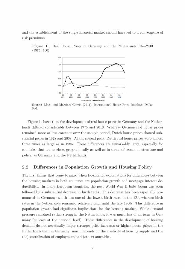
Figure 1: Real House Prices in Germany and the Netherlands 1975-2013(1975=100)

Source: Mack and Martinez-Garcia (2011), International House Price Database DallasFed.

Figure 1 shows that the development of real house prices in Germany and the Nether-

lands differed considerably between 1975 and 2013. Whereas German real house prices

remained more or less constant over the sample period, Dutch house prices showed sub-

stantial peaks in 1978 and 2008. At the second peak, Dutch real house prices were almost

three times as large as in 1985. These differences are remarkably large, especially for

countries that are as close, geographically as well as in terms of economic structure and

policy, as Germany and the Netherlands.

2.2 Differences in Population Growth and Housing Policy

The first things that come to mind when looking for explanations for differences between

the housing markets in both countries are population growth and mortgage interest de-

ductibility. In many European countries, the post World War II baby boom was soon

followed by a substantial decrease in birth rates. This decrease has been especially pro-

nounced in Germany, which has one of the lowest birth rates in the EU, whereas birth

rates in the Netherlands remained relatively high until the late 1960s. This difference in

population growth had significant implications for the housing market. While demand

pressure remained rather strong in the Netherlands, it was much less of an issue in Ger-

many (at least at the national level). These differences in the development of housing

demand do not necessarily imply stronger price increases or higher house prices in the

Netherlands than in Germany: much depends on the elasticity of housing supply and the

(de)centralization of employment and (other) amenities.

8

However, there also appears to be an important difference between the two countries

with respect to housing supply. Vermeulen and Rouwendal (2007) find that the price

elasticity of housing supply in the Netherlands is virtually equal to zero, whereas Lerbs

(2014) finds significant (both statistically and economically) effects of house prices on

construction activity in Germany. In other words: housing supply is more elastic in Ger-

many, which has a stabilizing effect on house prices. On the other hand, the combination

of growing demand and inelastic supply was probably an important driver of increasing

house prices in the Netherlands.

In addition to the difference in supply elasticities, there is an important difference in the

tax treatment of owner-occupation in the two countries that may play an important role.

Ever since the introduction of an income tax in the Netherlands in the early 20th century

interest paid on mortgage loans was deductible from taxable income.3 Initially, this was

motivated by the aim of treating owner-occupiers in the same way as homeowners who rent

out their property. That is, the rent foregone because of owner-occupation had to be added

to taxable income, and the mortgage interest paid was regarded as the cost associated

with the realization of this income-in-kind. Later on the motivation changed. Imputed

rental income was deliberately determined at a very low level to stimulate homeownership,

while at the same time (and for the same reason) mortgage interest deductibility was fully

maintained. This is in stark contrast to Germany where mortgage interest payments on

owner-occupied housing are not tax deductible.4 In Germany, deductibility of interest

paid is restricted to non-owner occupied real estate. Mortgage interest deductibility in

itself does not necessarily lead to higher house prices. It stimulates housing demand, but

if supply reacts swiftly, the price level does not have to change. However, in combination

with extremely price inelastic housing supply in the Netherlands this tax facility has

probably contributed substantially to the higher price level.

To complete the picture, some other factors have to be added. Both countries sub-

stantially differ in the way home ownership is stimulated. In the Netherlands the national

mortgage guarantee (abbreviated in Dutch as NHG) implies that the Dutch state guaran-

tees repayment of accepted mortgage loans to the lender. There is a one-time premium for

this insurance to be paid by the household, but it is very low and since mortgage suppliers

offer a slightly lower interest rate for insured loans, it typically is paid-back within a few

3Since approx. 2000 Dutch workers living in Germany can opt for the Dutch income tax system, whichimplies that they continue to be able to benefit from mortgage interest deductibility. See Section 4. Untilrecently this was possible with any type of mortgage, but at present mortgage interest deductibility fornew contracts has been restricted to fixed price and linear mortgages.

4Imputed rents also do not have to be added to taxable income in Germany, but we noted alreadythat in the Netherlands they are determined at a very low level. The tax rules in the Netherlands ensurethat the net effect of subtracting mortgage interest paid and adding imputed rent can never result in ahigher taxable income.

9

years.5 If a household qualifies for the guarantee, loan to value (LTV) ratios larger than

1 become possible – and are indeed common – as not only the full sales price of the house

but also the transaction costs involved can be financed by the insured mortgage loan.

The essential eligibility requirement is that the ratio between the mortgage payments and

household income should not be too high – typically the threshold is around 30% – and

that the workers in the household have job tenure.6

To see how this could contribute to the development of Dutch house prices shown

in Figure 1, consider for simplicity a household that takes an interest-only mortgage

loan. The maximum size L of the loan is given by the equation: iL = cY , where i is

the (net) interest rate, Y is household income from tenured jobs and c is the critical

share of mortgage payment in household income. Clearly, the maximum bid a household

can make for a house is equal to cY/i, a decreasing function of the interest rate i. In

the 1970s interest rates were relatively low and households could pay large amounts of

money for their houses. Around 1980 there was a shift towards a much tighter monetary

policy and initially the effect was that interest rates increased considerably, implying

much lower borrowing (and bidding) capacity of Dutch households.7 In the course of the

1980s and 1990s interest rates gradually decreased, while the increasing share of double

earner households8 and economic growth lead to significant increases in household income.

These developments contributed to the substantially higher borrowing capacity of Dutch

households. Since housing supply was essentially inelastic, the increased bidding capacity

did not lead to better or more luxury houses, but predominantly to higher prices for the

same houses. Note that in this analysis the possibility to realize high LTVs – which exists

in the Netherlands, but not in Germany – is essential, since the necessity to invest – say

– 20% of the value of the house from other sources (such as savings) would have made it

much more difficult for first-time Dutch buyers to pay the high prices.

In Germany the government encourages saving for house purchases through fiscal mea-

sures.9 There exists a contractual savings system allowing households to pin down future

interest rates on contracts for future lending for house purchases. Due to government

5This means that the premium is so low that the lower interest rate banks are willing to offer inreturn for the disappearance of the default risk is more than sufficient to pay it. This may raise doubtsabout the appropriateness of the level of the premium. The fact is that even in the current crisis thenumber of defaults has remained low and the NHG funds accumulated from past premiums paid havebeen sufficiently large.

6There is also an upper limit on the price of the house.7For the negative effect of monetary policy shocks on house prices, see e.g. Iacoviello (2005) and

Iacoviello and Neri (2010).8In the Netherlands the increase in female labor force participation occurred relatively late. Many

working women have a part-time job. Only in the course of the 1990 banks started taking into accountthe income of the second worker when determining a household’s borrowing capacity.

9Up till 2006 the government subsidized the first real estate purchase for all taxpayers. However, thissubsidy has been abolished in 2006.

10

subsidies these contracts offer favorable conditions compared to other types of lending.

On the other hand such subsidized contracts are conditional on the commitment to save

before obtaining the loan, reducing the required size of the loan and decreasing the LTV

ratio due to higher equity, which arguably has a stabilizing effect on house prices.

In addition, the difference in accessibility of the rental market between the two coun-

tries may have contributed further to the differential development of house prices. In

Germany the rental sector is large – 56% of households do not own their main residence

– and open to all households. In the Netherlands the rental sector is somewhat smaller –

43% of all households rent their main residence – and it consists predominantly of social

rental housing, which is rent-controlled. There is severe excess demand for social rental

housing, especially in the larger cities, and since the rationing systems favor lower in-

comes, households with higher incomes are therefore practically unable to rent. Unlike

in Germany, renting is therefore not a real alternative to owning for many Dutch house-

holds. Note that this contributes to making demand less price elastic than it would be if

the rental market offered a good substitute to owner-occupied housing.

3 The Model

3.1 The Model and its Implications for the Border Effect on

House Prices

To motivate the empirical work that follows, we now formulate a simple model that

incorporates some of the stylized facts discussed in the previous section. Assume that

Dutch workers are dispersed over a line with its origin in the center of the Dutch Randstad.

A position on the line is indicated by x, the residential location, or y, the location of the

worker’s job, and refers to the distance to the center of the Randstad. The line stretches

eastward and crosses the border with Germany in x. Jobs are present everywhere on

the line, and the density of labor demand g (x, w (x)) for Dutch workers is a decreasing

function of x until the German border.10 The decreasing density of labor demand reflects

that the Randstad is the urban heart of the Netherlands.

The density of housing at a particular location x is assumed to be an increasing

(housing supply) function si (p (x)) of the local housing price p (x), with i equal to N

on the Dutch side of the border and equal to G on the German side.11 We assume that

housing supply is less elastic in the Netherlands than in Germany. We interpret the

10That is ∂g/∂x < 0.11This formulation implies that the housing supply function is identical everywhere in a given country.

We discuss the implication of less elastic housing supply close to the Randstad toward the end of thissection.

11

housing price – in line with the economic literature – as the price of one unit of housing

services or – equivalently – as the price of a house with a given set of characteristics.12

The number of housing services consumed refers in this setup to the quality of housing

relative to that of the reference house.

The housing price p (x) refers to the value of all present and future housing services and

must be distinguished from the payment for user cost during one period, which are known

as the user cost. We adopt a simple formulation in which the user cost is the product of

the housing price and the net interest rate. In Germany the net interest rate equals the

gross rate since there is no mortgage interest deductibility, but in the Netherlands the net

interest rate is equal to the gross rate multiplied by one minus the marginal income tax

rate. We thus define the user cost of housing in Germany as ucG (p (x)) = ρ p (x), where

ρ is the mortgage interest rate, and in the Netherlands as ucN (p (x)) = (1− τ) ρ p (x),

where τ is the marginal income tax rate.

Worker utility is determined by the wage w (y) where y denotes the worker’s job lo-

cation, the user cost of housing uci (p (x)), where x denotes the residential location, the

commuting distance d (x, y) and a dummy variable f (x, y) that indicates that the com-

mute crosses the border: u = u (w (x) , uci (p (x)) , d (x) , f). We consider the distribution

of a given population of Dutch workers over jobs that are located in the Netherlands and

residential location in the Netherlands and – perhaps – also in Germany. We assume

throughout the paper that jobs in the Netherlands are all occupied by Dutch workers,

and that jobs in Germany are all occupied by German workers. An equilibrium in this

model is a distribution of the Dutch workers over job locations in the Netherlands such

that:

a) All Dutch workers are employed and housed.

b) The number of workers equals the demand for labor at the prevailing wage at each

location.

c) The number of houses equals the supply of housing at the prevailing user cost/housing

price.

d) All workers reach the same utility at the chosen residential and job location.

e) No worker is able to improve his utility by changing job location, residential location,

or both.

The first and second characteristics imply that we must have∫ x

0g (y, w (y))dy = B,

where B is the given size of the Dutch labor force. The first and third equations imply:

12The concept ‘housing services’ was introduced by Muth, Muth (1969).

12

∫ x

0sN (p (x))dx+

∫ x

xsG (p (x))dx = B, where x denotes the extent of the Dutch settlement

in Germany. If all Dutch workers live in their own country, x = x.

Suppose some Dutch workers live in Germany. Compare the worker who lives on the

Dutch side of the border, at x−dx, where dx is a small positive number, with the one who

lives at the German side at x + dx. Since neither should be able to gain from changing

their jobs their wages-net-of-commuting costs must be equal. The requirement that both

reach the same level of utility thus implies that the negative impact of crossing the border

must be completely compensated by the housing price. That is, the housing price must

show a discontinuity at the border that reveals the willingness to pay of a Dutch worker

to live in the Netherlands instead of Germany.

The jump in the housing price that occurs at the border has of course consequences for

the quantity of housing services demanded, which should increase. The value of the house

is affected by two components, quantity as indicated by the number of housing services

and price per unit of housing services. The border does affect both components differently.

At the border the price per unit of housing services decreases, and this affects the quantity

of these services demand by the households. If housing services are a normal good, the

two effects point in opposite direction and the sign of the net effect is undetermined.

However, the downward jump in the unit price should be expected to increase the number

of units consumed, which implies a better quality (=a larger number of housing services)

of housing at the German side of the border. It may also be noted that the impact of the

border on population density is indeterminate as the effect of the lower housing price and

the more elastic supply counteract each other.

3.2 Some Properties of the Equilibrium

In this subsection we explore some properties of an equilibrium when utility is Cobb-

Douglas:13

u = ln (w (y)− td (x, y))− α ln(uci (x)

)− βf (x, y) (1)

with α, β > 0. A stylized fact of commuting behavior in the Netherlands is that

commutes are predominantly into the Randstad area. This suggests that in equilibrium

we should have:

∫ x

0

g (z, w (z))dz ≥∫ x

0

s (p (z))dz (2)

13With these preferences, households spend a given share of their budget on housing services. Theirbehavior is therefore similar to what happen if a constraint imposed on the share of housing in totalexpenditure – imposed, for instance, by mortgage insurance – is valid.

13

for all x, 0 ≤ x ≤ x. Workers should therefore reach their highest possible utility

when commuting in western direction. A convenient way of modeling such a situation is

to assume that all workers – at any residential location – are indifferent between all jobs

located between their residential location and the Randstad center.14 It is easy to verify

that this is the case if the wage function satisfies:

w (y) = w (0)− t y. (3)

We require also that for any job location a worker is indifferent between all residential

locations that are further to the east. Standard calculations15 then show that:

p (x) =c (w (0)− tx)1/α

(1− τ) ρ0 ≤ x ≤ x (4)

where c is a constant of integration. The analysis of the previous section implies that

Dutch workers who live in Germany should pay:

p (x) =c (w (0)− tx)1/α e−β/α

(1− τ) ρx ≤ x ≤ x (5)

It can be verified that with these wage and housing price equations the conditions

d) and e) for equilibrium are fulfilled. In order to verify the validity of the other three

conditions, observe that labor demand in all locations is decreasing in w (0). We can

therefore find a labor market equilibrium in which all workers have a job and demand for

labor is satisfied at each location by choosing an appropriate value for w (0).

For housing we follow a similar approach. We assume that housing supply can be

described by a log-linear supply function:

QN (x) = σN0 p (x)σ

N1 (6)

Here Q refers to the number of housing services supplied. In order to find the density

of households we divide by individual demand for housing services, as follows from out

Cobb-Douglas utility function:

sN (x) = QN (x) /α (w (0)− tx)

(1− τ) ρ p (x)(7)

If all Dutch workers live in their own country, we must have:

14Compare the urban model with decentralized unemployment of Hamilton and Roell (1982).15Compare the monocentric model in which consumers have Cobb-Douglas preferences. The housing

price function (4) follows from the Muth condition ∂p/∂x = −t/s (p (x)). Substitution of the housingdemand function and solving the resulting differential equation gives the result.

14

∫ x

0

sN (p (x))dx = B . (8)

This condition allows us to compute the value of the constant of integration c in the

housing price Equation (4):

c = 1/

[1

B

σ0

(1 + σ1) t

1

(ρ (1− τ))σ1

[w (0)σ1/α − (w (0)− tx)σ1/α

]]1/(1+σ1)

(9)

After substituting this expression into the price function (4), we arrive at a price

equation that gives the local housing prices that solve the model conditional upon the

value of w (0) that equilibrates the labor market. In this equilibrium inequality (2) must

be satisfied, as is suggested by the stylized fact discussed above.

It can be shown that these local housing prices are everywhere increasing in the to-

tal number of workers B, the equilibrium wage w (0) and the marginal tax rate τ , and

decreasing in the interest rate ρ. The model is thus consistent with the story told above

about the pressure put on Dutch house prices. If house prices in an initial situation are

close on both sides of the border, all Dutch workers will live in their own country. If the

housing price on the Dutch side of the border increases relative to that on the German

side, nothing happens until the threshold that reflects the reluctance of the Dutch work-

ers to live among the Germans is exceeded. Then Dutch workers start buying houses in

Germany and the German housing price immediately across the border is described by

(5).

3.3 Extending the Model to Germany

A similar model as outlined for the Netherlands is assumed to hold on the German side

as well, for instance, the Ruhrgebiet playing the same role as the Randstad. Differences

between the countries are that the elasticity of housing supply, σ1, is higher in Germany

and that there is no mortgage interest deductibility. Depending on the parameters of the

model, the German housing price may be close to the Dutch one at the border, or differ

from it.

A major new element is, of course, that for Germany we should consider the possibility

of Dutch workers ‘invading’ the country. This situation will only occur, of course, if the

ratio of the Dutch and German housing price exceeds exp (β/α). Dutch workers will then

enter and overbid German workers close to the border. The consequence is that (at least)

close to the border the initial equilibrium is disturbed. All German workers now have to

be housed in a smaller amount of space, which calls for higher house prices. Some German

workers now have to commute in reverse direction, that is towards the Dutch border. That

15

means that – at least close to the border – the equilibrium will be qualitatively different

from that discussed in the previous section does not exist.

Unless the spatial pattern of house prices changes, the displaced German workers now

have to pay a higher housing price or face a longer commute. Interest in jobs close to

the Dutch border will therefore disappear unless wages become higher, but this means

that the number of jobs will decrease. The geographical distribution of German jobs

will therefore change. It is possible that an equilibrium emerges in which the German

workers can be divided into two groups: group 1 commutes in the direction of the Dutch

border, whereas group 2 commutes in the opposite direction. For group 2 the equilibrium

is similar to that in the situation in which no Dutch workers live in Germany. For group 1

the equilibrium is close to that on the Dutch side of the border: all workers are indifferent

between all jobs that are between their residential location and the Dutch border because

the wage compensates the commuting cost. However, in contrast to the situation in the

Netherlands, the density of jobs is increasing if one moves from west to east. This situation

is illustrated in Figure 2.

Figure 2: House Prices, Location Patterns and Commuting close to the Border

Note: The arrows show the direction of the commutes. x location of the border. x extentof Dutch workers living in Germany. x German workers living in Germany.

This figure shows that to the left of the Dutch/German border at x Dutch workers

commute in the direction of the Randstad, as is indicated by the arrow. To the right

of the German border Dutch households live until x, and they commute to jobs in the

Netherlands. The jobs that are located between x and x are occupied by German workers

who live between x and x, they commute in the direction of the Dutch border. The

workers who live in that area between x and x also occupy all jobs that are located there.

This means that the presence of Dutch workers in Germany results in an extension of

the Dutch commuting and housing price patterns to a wider area then where the Dutch

workers are actually settled. Only to the right of x the pattern that is present everywhere

16

in the German part of the Figure when the Dutch do not cross the border still holds.16

Finally, we note that a crucial property of the model developed in this section is that

commuting costs are linear in distance. Although we think this is a useful approximation

for most commutes, it is unlikely to be true for longer commutes. For instance, there will

hardly be any Dutch worker living close to the German border who is happy to accept a

job in Amsterdam. After a certain threshold – often thought to be close to 45 minutes

travelling – commuting costs increase more than proportional with distance. This means

that the rent gradient may become steeper if workers start to live further from their jobs,

possibly on the other side of the German border.

4 Development of Dutch House Prices close to the

German Border

With house prices more or less stable in Germany and rapidly increasing in the Nether-

lands over much of the aforementioned period, we are especially interested in the devel-

opments of real estate prices on the Dutch side of the border and whether price increases

vary with the distance to the Dutch-German border. Therefore, we estimate a hedo-

nic price function on Dutch housing transactions in the period January 1985-June 2013

within 50 km of the German border. The data refer to transactions handled by mem-

bers of the Dutch Association of Real Estate Brokers, abbreviated in Dutch as NVM. We

use a large number of transaction and housing characteristics to control for differences in

housing quality (e.g., surface area, quality of maintenance, house type). Further, we use

municipality-dummies to control for all kinds of local characteristics that remain constant

over time as ‘fixed effects’, the distance to the German border to see if house prices are

lower close to the border, and time dummies.

After cleaning the data 853, 807 transactions remain available for our semi-logarithmic

regression analysis.17 Table 1 lists the descriptive statistics of the dataset. Estimation

results for the time dummies and their interaction with the distance to the border are

shown in Figure 3. The dependent variable is the log of the transaction price. The full

set of estimation results is reported in Table A1.

16The figure assumes that commuting costs are identical for Dutch and German workers. Many Dutchemployers reimburse commuting costs, whereas this practice does not seem to be present in Germany.If commuting costs are higher in Germany, the German housing price function would be steeper, butqualitatively nothing would change in the Figure.

17We started with 1, 001, 757 observations and removed observations with missing and/or incorrectvariable values, as well as building lots, garage boxes, house boats, caravans, recreational property,countryside estates, partially rented houses, not permanently occupied objects and real estate investmentsobjects.

17

Table 1: Descriptive Statistics for all Variables in the 50km wide Study Area(Period: 1985–2013)

Variable Min Max Median Mean Std. Dev.

Transaction price (x 1,000 Euros) 10 2200 158 182 121Transaction price corrected for inflation (x 1,000 Euros) 11 2596 192 221 134Surface area (m2) 26 537 120 128 45Transaction price per square meter (x 1,000 Euros/m2) 0.079 5 1.387 1.413 0.691Parcel size (m2) 0 99845 206 536 2108Number of rooms 1 30 5 4.602 1.354Distance to Germany (km) 0 50 27.449 26.108 14.947Nat. log of Trans. price corr. for inflation (x 1,000 Euros) 9.348 14.77 12.163 12.161 0.537Transaction characteristicsAnnual time dummies: see below 0 1Free of transfer tax (0=no/1=yes) 0 1 0 0.0155 0.1234Structural characteristicsNatural log of surface area (m2) 3.258 6.286 4.787 4.802 0.323Natural log of parcel size (m2) (0 in case of apartment) 0 11.511 5.328 4.786 2.220Natural log of number of rooms 0 3.401 1.609 1.483 0.304Heating system: present (0/1) 0 1 0.970 0.170Garden: absent (0/1) 0 1 0.020 0.140Garden: present (0=no/1=yes, simple or normal) 0 1 0.652 0.476Garden: present (0=no/1=yes, well-kept) 0 1 0.328 0.470Parking place: absent (0/1) 0 1 0.473 0.499Parking place: present (0/1) 0 1 0.047 0.212Parking place: garage and/or carport present (0/1) 0 1 0.480 0.500Inside maintenance: bad to moderate (0/1) 0 1 0.004 0.059Inside maintenance: mediocre to fair (0/1) 0 1 0.118 0.323Inside maintenance: good to excellent (0/1) 0 1 0.878 0.327Outside maintenance: bad to moderate (0/1) 0 1 0.003 0.056Outside maintenance: mediocre to fair (0/1) 0 1 0.104 0.305Outside maintenance: good to excellent (0/1) 0 1 0.893 0.309Isolation: absent (0/1) 0 1 0.183 0.387Isolation: 1 or 2 types present (0/1) 0 1 0.447 0.497Isolation: 3 or more types present (0/1) 0 1 0.370 0.483Building age dummies (0/1), ranges: 1500-1905; ’06-’30; ’31-’44; ’45-’59; ’60-’70; ’71-’80; ’81-’90; ’91-2000; >2000House type dummies (0/1), indicating any of the 15 possible types (8 types of houses, 7 types of appartments)Spatial characteristicsMunicipality dummies 0 1 - -Year dummies (range 1985–2013) * dist. to Germany (km) 0 50 - -

Variable Mean Std. Dev. Variable Mean Std. Dev. Variable Mean Std. Dev.

1985 0.014 0.117 1995 0.029 0.167 2005 0.056 0.2301986 0.017 0.128 1996 0.033 0.179 2006 0.057 0.2321987 0.017 0.128 1997 0.037 0.189 2007 0.059 0.2351988 0.017 0.130 1998 0.043 0.203 2008 0.050 0.2181989 0.018 0.132 1999 0.043 0.204 2009 0.038 0.1901990 0.017 0.129 2000 0.045 0.206 2010 0.039 0.1931991 0.018 0.135 2001 0.050 0.218 2011 0.036 0.1861992 0.019 0.138 2002 0.050 0.219 2012 0.038 0.1911993 0.022 0.146 2003 0.051 0.220 2013 0.015 0.1211994 0.021 0.144 2004 0.052 0.222

Note: italic variables are not used in the regression model

18

Figure 3: Development of the Dutch Housing Price near the German Border

Figure 3 shows the development of Dutch house prices close the border as implied

by the estimation results.18 House prices at the border, indicated by the time dummy

coefficients, have increased considerably over time with a peak in 2008, when the financial-

economic crisis started to affect the Dutch housing market. House prices 50 km inside the

Netherlands are always higher than at the border, which is in line with our model. How-

ever, around 2000 the discrepancy between the two series is growing, probably reflecting

the stronger impact of the proximity to the German border as we discuss below.

Figure 4 illustrates the development of the price gradient over time.19 It shows that the

gradient remained more or less constant between 1987 and 2004, then increased until 2008,

probably in reaction to the migration of Dutch households to Germany, and has stabilized

at this higher level since then. The model developed in the previous section suggests that

this gradient reflects commuting costs, but the shift to a higher level since 2005 must

probably be interpreted as a short or medium run reaction to the higher numbers of

Dutch workers moving across the border and thus relieving pressure on the Dutch house

prices close to that border.

Since Germany and the Netherlands are both members of the European Union and

both have signed the Schengen Treaty, the border between the two countries is easy

to cross. Moreover, since 2001 Dutch citizens who have a job in the Netherlands can

opt for the Dutch income tax even if they live across the border in Germany.20 This

means that Dutch migrants can take the mortgage interest deductibility with them as

18Figure 3 is based on the coefficients for the time dummies as reported in (the southeast part of) TableA1. The price index is constructed as exp (co (year)), where co (year) is the estimated coefficient for thetime dummy referring to the year.

19Figure 4 gives the coefficients of the time * distance interactions reported in (the southwest part of)Table A1.

20This is also the case for Dutch households living in Belgium and other countries. The general principlefollows from jurisprudence at the European level in the 1990s according to which workers living abroadmust (have the possibility to) be taxed in the same way as those living in the country in which their jobis located. The so-called ‘keuzeregeling’ (choice possibility) is included in article 2.5 of the Dutch incometax law of 2001.

19

Figure 4: Change in Price Gradient within 50 km of the Dutch-German Border

long as their job remains in the Netherlands. This change in tax treatment facilitates

arbitrage considerably. Figure 5 shows the development of cross county migration between

the Netherlands and Germany in the period 1974-2012. It is striking that there is a

considerable net migration from the Netherlands to Germany starting in the early 2000s,

when Dutch house prices increased rapidly and it became possible for Dutch workers to

take advantage of mortgage interest deductibility even when moving across the border.

This development is in line with numerous newspaper reports in the early 2000s concerning

Dutch citizens who had moved just across the German border to live in a much larger

house for the same or even a lower price. After a temporary drop, net migration to

Germany increased again in 2010.

Figure 5: Bilateral Migration, Netherlands and Germany, 1974-2012

Source: Destatis.

Summarizing, it may be stated that Dutch house prices in the border region increased

substantially in the period 1985–2013, but less in areas that were close to the German

border and least at the border itself. Especially since 2000 the Dutch seem to have become

aware of the potential attractiveness of moving across the German border, and this has

contributed to the divergence between house prices at the border and at a 50 km distance

20

of the border.

5 Data on House Prices on Both Sides of the Border

2007-2011

In this section we compare house prices on both sides of the border. As information on

German house prices is available starting in 2007 we restrict the analysis to the years

2007-2011.21 In Germany we observe houses that were offered on the website of Immo-

bilienScout24. This website allows realtors as well as private sellers to offer their real

estate for sale or rent. It is the largest and most frequented internet real estate market

place in Germany. ImmobilienScout24 estimates that about 50% of all real estate objects

offered for sale or rent in Germany are offered via their website Georgi and Barkow (2010).

Since transaction values are not observed, we use the last price for which the house was

offered on this website.

In the Netherlands we observe houses that were offered on the FUNDA website by

realtors that are members of the NVM. FUNDA is the largest website for houses in

the Netherlands. It only registers houses offered for sale via members of NVM, which

means that approximately 70% of the national supply is offered on this website. However,

this share differs across regions. To make the data comparable with those available for

Germany we do not use information on transaction values, but only the last observed

price on the FUNDA website. Moreover, for the same reason we add information about

Dutch houses that have been withdrawn from the FUNDA website without being sold.

Using ask prices instead of observed transaction prices is of course an additional source

of uncertainty. To our knowledge, there is one study investigating the difference between

the last observed ask price of objects advertised at ImmobilienScout24 and actual trans-

action price in Germany. For rural regions in Rhineland-Palatine Dinkel and Kurzrock

(2012) find a difference of about 15%. To relate this to the Dutch dataset, where the trans-

action price is available to us, we compute the difference between the last ask price and the

transaction price for all objects within 10km to the German border. In the Netherlands

the discount seems to be substantially smaller, only about 5% of the transaction price.22

Using this dataset, we employ a method proposed by (Black 1999) to measure the

impact of the border on house prices by concentrating on the border region. We only

include objects located within a distance of 10km of the German-Dutch border in our

analysis to guarantee that objects far away from the border do not distort the analysis.

21For a description of the dataset see an de Meulen et al. (2014).22In the computation of the average percentage price difference we exclude the highest and lowest one

percent to eliminate faulty entries.

21

Table 2: Descriptive Statistics

Netherlands Germany Difference

0–5 km 5–10 km 0–5 km 5–10 km 0–5km 5–10 km

Observations 117,992 52,711 13,656 9,561Price 241,723 261,446 218,740 218,377 22,983*** 43,069***

(393) (617) (867) (1077) (952) (1241)Living space (m2) 140 143 145 145 -5.21*** -2.50***

(0.14) (0.22) (0.38) (0.48) (0.41) (0.52)Number of rooms 5.4 5.3 5.2 5,2 0.19*** 0.11***

(0.0048) (0.007) (0.0131) (0.0151) (0.014) (0.0200)Lot size (m2) 642 635 683 628 -41.15*** 6.94

(3.92) (5.85) (5.8) (5.78) (7.00) (8.22)Year of construction (in percent)1500-1905 3.51 4.41 2.39 3.01 1.12*** 1.40***

(0.0014) (0.0020)1906-1930 9.65 10.52 6.44 5.61 3.21*** 4.92***

(0.0023) (0.0027)1931-1944 5.82 7.84 2.78 2.53 3.04*** 5.31***

(0.0016) (0.0020)1945-1959 12.11 9.74 11.46 9.47 0.65** 0.28

(0.0029) (0.0033)1960-1970 16.44 16.91 13.88 13.43 2.56*** 3.48***

(0.0031) (0.0039)1971-1980 22.62 17.18 13.57 13.12 9.05*** 4.07***

(0.0032) (0.0038)1981-1990 11.84 11.81 9.97 9.25 1.86*** 2.57***

(0.0027) (0.0033)1991-2000 10.62 12.82 13.91 15.08 -3.28*** -2.26***

(0.0031) (0.0039)2001-present 7.39 8.76 25.6 28.51 -18.21*** -19.75***

(0.0038) (0.0048)Last observed in (in percent)2007 23.31 23.38 15.95 17.3 7.36*** 6.08***

(0.0034) (0.0043)2008 21.91 22.29 18.91 22.13 3.00*** 0.15

(0.0036) (0.0046)2009 18.19 19.07 21.54 18.7 -3.34*** 0.37

(0.0037) (0.0043)2010 17.95 18.2 21.19 21.52 -3.25*** -3.33***

(0.0037) (0.0045)2011 18.64 17.07 22.41 20.34 -3.77*** -3.27***

(0.0037) (0.0044)House typeTerraced house 38.03 37.44 9.18 10.99 28.86*** 26.45***

(0.0028) (0.0038)Corner house 19.35 19.89 25.45 28.79 -6.10*** -8.91***

(0.0039) (0.0049)Detached house 42.62 42.67 65.37 60.21 -22.75*** -17.54***

(0.0043) (0.0054)

Notes: *, **, *** indicate differences are significant at the 10%, 5% and 1% level.Standard deviations reported in brackets. Observations have been excluded if: price,living space, lot size, number of rooms < 1. Additionally to that, the top and bottom1% of price, living space and lot size as well as the top 1% for the number of roomshave been excluded.

22

The number of observations on the Dutch side of the border is substantially higher: the

portion of Dutch houses to German ones in the datasets is about 7 : 1. This large difference

might be due to several causes. First, market coverage of ImmobilienScout24 in Germany

is about 50%, which is lower than the one of the NVM in the Netherlands (70%). Second,

it might be due to differences in the average time till a given object is offered for sale

again. In Germany house owners are incentivized to hold on to their properties, as they

have to pay taxes on speculative gains, if a house is sold within ten years of the purchase.

Third, because of the large rental market in Germany, potential buyers that are not sure

about their future household size or whether they will stay in the same city might be

tempted to rent instead of buy as renting is associated with lower costs of relocation.

In the Netherlands, this mechanism does not work because entrance to the social rental

sector is limited, and a private rental market is virtually absent. Finally, there could be

differences in population density on both sides of the border. To investigate the latter

issue we have collected data on population density which is presented in the map in Figure

A1. It appears that for most parts of the border population densities are comparable on

the German and the Dutch side.

Apart from the last observed list price, the two datasets provide information about

several other housing characteristics. Included in both datasets are living space, lot size

(both in square meters), number of rooms, year of construction23, house type24, the last

time an object has been advertised, and the location. We report some descriptive statistics

for these variables in Table 2. There, we divide the dataset for objects that are located

within 5 kilometer distance to the German-Dutch border as well as objects further away

(5km-10km) for both countries.

The descriptive statistics show the presence of statistically significant price differences

between houses on both sides of the border. On average house prices of objects within

a boundary of five kilometers to the Dutch-German border are about 23 thousand Euros

more expensive in the Netherlands than in Germany. The difference is larger if we also

consider houses at a distance between 5 and 10 km, because Dutch house prices are higher

in that area. Additionally to that, houses in the Netherlands are slightly smaller (in terms

of living space and lot size) and less recently build, implying that the price mark up for

identical houses might be even more pronounced.

The differences in the amount of living space and lot size are consistent with the

urbanization patterns on both sides of the boundary documented in Tennekes and Harbers

23The year of construction is available for 9 time periods. These consist of the years from ‘1500-1905’,‘1906-1930’, ‘1931-1944’, ‘1945-1959’, ‘1960-1970’, ‘1971-1980’, ‘1981-1990’, ‘1991-2000’, and ‘2001 untilpresenT’.

24Due to differences in house types in Germany and the Netherlands we include the categories terracedhouse, corner house, and detached house.

23

(2012). The explanation for the difference in the year of construction, shown in Figure

6, is less clear. One explanation could be the longer holding period for German home

owners. Given each object is first observed when it is sold after construction has finished,

a longer holding period implies that houses appear less frequent on the market resulting

in a relatively larger share of newly build houses.

Figure 6: Number of Observations by Year of Construction

Source: FUNDA, ImmobilienScout24, own calculations.

6 Analysis

In this section we report the results of three analyses, each one tackling a different aspect

of the problem. We start with a hedonic price function analysis. Then we consider

regression discontinuity analysis. And finally we carry out a spatial matching analysis. In

Section 6.4 we discuss the development of the border gap over the period 2007–2011, in

Section 6.5 we analyze regional differences.

6.1 Hedonic Price Analysis

Hedonic theory implies that the quality of a good is determined by the bundle of its

defining characteristics. By estimating a hedonic function we are able to extract the

implicit value of each characteristic of a house.

ln p = ZβZ + LβL + fβG + ε (10)

In Equation (10) ln p is a vector of logarithmic house prices, Z a matrix of the in-

dividual houses’ characteristics as described in Section 5 and βZ the characteristics’ im-

plicit prices. The matrix L represents location specific information, which consists of

two components. First, there is a dummy variable indicating a border segment. As the

24

Dutch-German border stretches out over about 500km, house prices might differ substan-

tially with respect to the location within one country. For instance, house prices on the

southern end of the border, with the employment centers Maastricht and Aachen, might

be higher than in the less densely populated regions in the north. We have therefore

divided the border into segments of 1km length25 and we include a dummy indicating

the nearest border segment into the regression equation. Second, we include the distance

to the border in polynomial form to deal with the possible impact of proximity to the

border on housing prices in a flexible way. In Table 3 below we report the estimation

results for the specification with polynomials up to the power four. Figure 7 shows the

results of the different estimated price effects of the distance to the boundary. The vector

f contains dummy variables that are equal to 1 for houses located in Germany and zeroes

for Dutch houses. The coefficient βG is the price markdown for objects in Germany and

the coefficient of interest in this analysis. We estimate the equation including all houses

within ten kilometers to the Dutch-German border.

All estimation results reported in Table 3 are in line with the intuition. Larger houses

are more expensive than small ones. A one percent increase in living space increases house

prices by about 0.6%. The price increase for one percent additional lot size is considerably

smaller (0.2%). The house type also has a substantial impact on the price. Given the

reference category, detached houses, corner houses are subject to a price markdown of

about 20%, terraced houses an even larger markdown of about 25%. Houses that have

been built most recent are the most expensive. The price markdown for older houses

increases monotonically till 1940. The markdown for objects build in the intra war period

is less pronounced.

The estimated coefficient for the dummy variable βG, which indicates whether or not

the object is located in Germany, is highly significant. Houses in Germany are roughly

15% cheaper than their counterparts of identical quality on the Dutch side. Additionally

to this direct effect, the border seems to impact house prices in another way. In the

Netherlands, house prices decrease with decreasing distance to the German border.

To illustrate this we report the impact of the distance to the Dutch-German border on

house prices in Figure 7. The different lines represent the impact based on the different

estimations. First, assuming a linear relationship only, then stepwise including an addi-

tional polynomial. This convergence on the Dutch part seems robust to the inclusion of

additional polynomials. However, it cannot be found on the German side, as one might

have expected prices to increase with decreasing distance to the Netherlands.

25This results in a total of 490 border segments with a length of 1km in the estimation of Equation(10).

25

Table 3: Hedonic Regression

linear Quadratic cubic quartic

Average border effect (βG) -0.2279*** -0.2102*** -0.1500*** -0.1510***0.0046 0.0062 0.0081 0.0101

Distance Germany 0.0078*** 0.0047* -0.0315*** -0.00180.0008 0.0027 0.0065 0.0129

Distance Netherlands -0.0192*** -0.0309*** -0.0697*** -0.0962***0.0004 0.0012 0.0027 0.0053

(Distance Germany)2 0.0004 0.0101*** -0.0040.0003 0.0016 0.0055

(Distance Netherlands)2 -0.0014*** -0.0117*** -0.0237***0.0001 0.0007 0.0022

(Distance Germany)3 -0.0007*** 0.0017*0.0001 0.0009

(Distance Netherlands)3 -0.0007*** -0.0027***0.00005 0.0003

(Distance Germany)4 -0.0001***0.00005

(Distance Netherlands)4 -0.0001***0.00002

Living space 0.5899*** 0.5901*** 0.5898*** 0.5899***0.0021 0.0021 0.0021 0.0021

Lot size 0.1859*** 0.1860*** 0.1859*** 0.1858***0.0009 0.0009 0.0009 0.0021

Number of rooms 0.0085*** 0.0085*** 0.0086*** 0.0086***0.0003 0.0003 0.0003 0.0003

Terraced house -0.2469*** -0.2467*** -0.2463*** -0.2466***0.0017 0.0017 0.0017 0.0017

Corner house -0.2001*** -0.2000*** -0.1996*** -0.1998***0.0016 0.0016 0.0016 0.0016

Adj R-squared 0.8262 0.8263 0.8265 0.8266Observations 193920 193920 193920 193920

Note: *, **, *** indicate significance at the 10%, 5% and 1% level. Ad-ditional control variables are the year of construction (8 dummy variables:‘1500-1905’; ‘1906-1930’; ‘1931-1944’; ‘1945-1959’; ‘1960-1970’; ‘1971-1980’;‘1981-1990’; ‘1991-2000’; reference category is ‘built after 2000’) and dummyvariables for the border-segment (a total 490, each one with a length of 1km).

26

Figure 7: Price Effect of Distance to Boundary

Note: Negative values for distance indicate the Dutch side of the border, positive valuesthe German one. Source: FUNDA, ImmobilienScout24, own calculations.

6.2 Regression Discontinuity Design

A potentially attractive alternative to a hedonic analysis would be the regression disconti-

nuity analysis (see e.g. Imbens and Lemieux (2008)).26 The sharp regression discontinuity

design (SRD)27 is especially useful to estimate causal effects of a treatment, assigned on

the basis of an observable forcing variable, in our case the German-Dutch border. How-

ever, an important condition for the SRD to uncover the causal effect of – in our case –

the border is that all other variables that have an impact on house prices, notably housing

characteristics, are continuous functions of the distance to the border. Discontinuities in

such variables at the border imply a violation of the key assumption of SRD, viz. that the

treatment and the counterfactual are identical with respect to all other variables. Since

Tennekes and Harbers (2012) and the descriptives provided in Table 2 above suggest the

presence of structural differences in the housing markets of the two countries that are

probably reflected in discontinuities at the border, we first investigate this issue.28

It is conventional to present figures for the control variables to check the validity of

the continuity assumption. Since this would result in a large number of graphs, we only

used SRD as a descriptive device to investigate the presence of discontinuities in control

variables at the border. The results are reported in Table 4. Each line of this table gives

the impact of the border in a separate SRD regression.29 For instance, the first line refers

to a regression of the log of living space, the second to a similar regression on the log of

26See Keele and Titiunik (2013) for a discussion of RDD in a spatial context.27For a discussion of RD in economics see Lee and Lemieux (2010).28To estimate the boundary effect by SRD we use the code by Nichols (2007).29The bandwidth is computed according to Imbens and Kalyanaraman (2012). Similar to the estimation

of the hedonic price function we only include observations within 10 km to the boundary.

27

the lot size, et cetera. The table shows that for most of the variables that we used in the

hedonic regression there is a significant discontinuity at the border, which confirms the

differences in land use on both sides of the border that were observed by Tennekes and

Harbers (2012).

Table 4: SRD for Covariates

Variable Boundary effect Standard error

Log (living space) 0.0331*** 0.0081Log(lot size) 0.4876*** 0.0328Number of rooms -0.2407*** 0.0329House typeTerraced house -0.2804*** 0.0109Corner house 0.02767* 0.0157Detached house 0.2487*** 0.022Year of construction1500-1905 -0.0504*** 0.00871906-1930 -0.1063*** 0.01361931-1944 -0.0289*** 0.00641945-1959 -0.0056 0.01281960-1970 0.0446*** 0.01011971-1980 0.0364 0.02351981-1990 0.0499*** 0.00971990-2000 -0.0117 0.00882000-2011 0.1090*** 0.0127

Log (price) 0.0192 0.0127

Note: *, **, *** indicate significance at the 10%, 5%and 1% level. Positive coefficients indicate that houseson the German side do exhibit more units of the re-spective variable. For the binary variables, house typeand the year of construction, positive coefficients in-dicate that the variety is more probable to be foundin Germany.

Frolich (2007) has investigated situations like the one encountered here where some

housing characteristics differ between treated and non-treated objects and suggests con-

trolling for additional covariates to reduce estimation bias. We therefore estimate the

boundary effect on house prices using SRD controlling for various covariates30 using the

STATA code by Nichols (2007).31 Doing so, we find a jump in house prices at the bound-

30The included covariates are: Log(lot size), log(living space), nine dummy variables for the year ofconstruction, three dummy variables for the house type, five dummy variables for the year of transaction,and 56 dummy variables for the border segment closest to the individual house. The 56 border segmentsrepresent border bits, each of ten kilometers length.

31As we expected, results including covariates differ substantially from the results excluding them. Thisdiffers from the general experience in which covariates are continuous in the forcing variable, see Section5.2 of Imbens and Kalyanaraman (2012). If we don not include covariates we do not find a significanteffect of the border.

28

ary of 16.5%, as shown in the line with the bold figures in Table 5. The effect is highly

significant and very similar in magnitude to that found in the hedonic analysis when the

impact of the distance to the boundary is taken into account in a flexible way. To test

whether this discontinuity is unique at the border or potentially artificial to the datasets

we repeat the estimation setting spurious cutoff points. We estimate the equation for the

spurious cutoffs 2 km, 4 km, and 6 km on both sides of the border. The results, which

are also reported in Table 5, confirm that the discontinuity is unique to the border.

Table 5: Estimation Results SRD with Covariates

Distance to cutoff Boundary effect Standard error

6 km on the Dutch side 0.0059 0.0054 km on the Dutch side 0.0082* 0.00452 km on the Dutch side 0.0017 0.0046Border -0.1650*** 0.00882 km on the German side 0.0164 0.0114 km on the German side -0.0027 0.00976 km on the German side 0.0086 0.0098

Note: *, **, *** indicate significance at the 10%, 5% and 1% level.Positive coefficients indicate higher prices in Germany. The includedcovariates are: Log(lot size), log(living space), nine dummy variables forthe year of construction, three dummy variables for the house type, fivedummy variables for the year of transaction, and 56 dummy variablesfor the border segment closest to the individual house. The 56 bordersegments represent border bits, each of ten kilometers length.

We have also carried out an SRD analysis on the housing prices close to the border

without controlling for housing characteristics. We then find an insignificant effect of the

border. This tells us that the value of houses on both sides of the border is essentially

equal, suggesting that the negative impact of the border on the housing price is fully

compensated by the increase in the quantity of housing services consumed. This result is

consistent with the Cobb-Douglas specification of preferences used in Section 3.

6.3 Spatial Matching

Even though we only include objects within a certain threshold distance to the boundary

in the hedonic analysis, a concern one may have is that it refers to the whole German-

Dutch border and thus compares houses that may be hundreds of kilometers apart. Our

use of fixed effects for small border segments may not be sufficient to capture regional

differences correctly. Therefore we use matching techniques as an additional device to test

for the presence of border effects, as this allow for a comparison of objects that are more

or less directly adjacent. In a first step we match all objects on the German side to its

closest geographical neighbor on the Dutch side. We do this separately for each year to

29

exclude the impact of price differences between Dutch and German houses over time.32

Using these pairs of observations we compute differences for all explanatory variables.

We subtract the characteristics of the Dutch houses from their closest German counterpart,

positive values indicating that e.g. floor size in the German houses is larger than in the

Dutch ones.33

We test if these differences in quality persist even when looking at objects that are

spatially close. Figure 8 shows the percentage differences for the continuous explanatory

variables living space and lot size. While differences in living space do not seem to

be driven by the country, lot sizes of spatially close objects are substantially larger in

Germany. This implies that even spatially close houses that were observed in the same

year, need to be quality adjusted when compared, as we did in our regression discontinuity

analysis.

Figure 8: Difference in Lot Size and Living Space

Notes: Houses within 3km distance. Source: FUNDA, ImmobilienScout24, own calcula-tions.

We estimate the hedonic price function:

Δ ln p = βG +ΔZβx + ε (11)

where Δ ln p represents a vector of log price differences and matrix Z differences in the

two matched objects’ characteristics. Negative values for the coefficient βG indicate that

prices in Germany are lower than in the Netherlands. ε is an error term. We report the

estimation results in Table 6.

32The Stat module GEONEAR (Picard 2010) has been used.33For the variables in price, living space and lot size we build the log difference. For the three dummy

variable representing the house type we build three new variables, one for a matched pair consisting ofa terraced house and a corner house, one for a pair of a terraced house and a detached house and onefor a pair of a corner house and a detached house. For pairs of similar house types the all of the threevariables are assigned zero. For differences in the year of construction, we only observe time periods wecan control for by dummy variables for the Dutch side, we subtract the time periods means. For thedummy representing houses built before 1906 we set the value to 1900.

30

Table 6: Matched Pair Regression

Difference in 1km 2 km 3km

Average border effect (βG) -0.18*** -0.17*** -0.17***(0.06) (0.03) (0.02)

Living space 0.61*** 0.38*** 0.60***(0.11) (0.06) (0.04)

(Living space)2 -0.34** 0.02 -0.03(0.14) (0.07) (0.05)

Lot size 0.24*** 0.34*** 0.34***(0.06) (0.02) (0.02)

(Lot size)2 -0.05* -0.06*** -0.07***(0.03) (0.01) (0.01)

Number of rooms 0.0002 0.0098** -0.0032(0.0077) (0.0043) (0.0031)

Year of construction 0.0087*** 0.0071*** 0.0072***(0.0013) (0.0006) (0.0004)

(Year of construction)2 -0.000063*** -0.000036*** -0.000042***(0.000018) (0.000008) (0.000006)

Terraced, corner house -0.18*** -0.09*** -0.18***(0.05) (0.03) (0.02)

Terraced, detached house -0.42*** -0.26*** -0.30***(0.04) (0.02) (0.02)

Corner, detached house -0.18*** -0.17*** -0.14***(0.05) (0.02) (0.01)

Distance to match -0.08 -0.01 -0.03***(0.08) (0.02) (0.01)

Adj R-squared 0.65 0.67 0.67Observations 391 1631 3842

Note: *, **, *** indicate significance at 10%, 5%, and 1% level. Stan-dard errors in brackets underneath.

31

Houses on the Dutch side seem to be about 17% more expensive than otherwise com-

parable houses in Germany. The results are robust to altering the maximum distance

between two houses. Also,the estimated price effect of about 17% is perfectly in line with

the result of the hedonic regression (about 15%) and the SRD analysis (16%). The values

of the other coefficients are also in line with intuition. Larger houses, in terms of lot size

and living space, and newer houses are more expensive. The hierarchy of different house

types is detached houses, corner houses, and terraced houses with detached houses the

ones most favored.

6.4 House Price Development over Time

In the previous three subsections we have presented a consistent set of results that show

the presence of a considerable gap between quality-adjusted house prices on both sides of

the Dutch-German border. Earlier we suggested interpreting this difference as reflecting

the value of remaining in the Dutch social and cultural environment. If this interpretation

is correct, one would expect the boundary gap to be relatively constant over time as long

as the house price difference between the Netherlands and Germany remains substantial.

The reason is that the cultural differences change only slowly over time.

Figure 1, which depicts the all-country price indices in (Mack and Martinez-Garcia

2011), shows that real house prices in the Netherlands started to decline substantially

in 2008, while prices in Germany slightly increased. Figure 3 makes evident that this

also holds true for Dutch houses close to the German border. If our interpretation is

correct, we thus would expect the price difference at the border to be constant despite

the decreasing trend in the Dutch house prices.

By allowing for time variation in the price markup of Dutch houses over the years

and re-estimating Equation (11), we find that the price difference at the border has been

relatively stable (Table A2). Depending on the estimation sample, the absolute change in

the price difference has been 10% for the estimation using all objects within 1km and 2km.

For the estimation using all houses within 3km, which considerably increases sample size

and this way also the reliability of the results, the difference between the highest and the

lowest estimate for the price markup is only 6%. This is substantially lower than what

the development of the all country indices would imply. Assuming the price markup is

by about 17% on average, the price markup for Dutch houses should have decreased from

about 23% in 2008 to 9% in 2011, resulting in an absolute change of the price difference

of about 14%.

32

6.5 Regional Differences

Let us finally take a look at differences in house prices at different locations. We therefore

divide the border into three segments. If we follow the border starting in the north, the

first segment consists of the first 200km, the second one of the next 200km and the third

one of the remaining 156km. We then assign each of the matched pairs as explained in

Section 6.3 to a border segment, depending on the closest segment of the house located

in Germany. Table 7 shows the number of matched pairs in the different groups for the

three samples of all objects within 1km, 2km, and 3km. This shows that the number of

observations in the north is substantially lower than in the more urban environment in

the South, which also has been indicated by Figure A1.34

Table 7: Number of Observations in Different Border Groups

1km 2km 3km

0km - 200km 23 130 279200km - 400km 70 272 1,230400km - 556km 297 1,220 2,318

In our regional analysis we focus on the 3km sample as the number of observation

in the Northern group seems too low to get reliable estimates for the price effect in

the 1km and 2km samples of matched pairs. We re-estimate Equation (11) allowing for

different price effects for the three border segments. The results show the price difference

is substantially more pronounced in the Northern part of the border (Table 8). One

explanation for these different effects of the national border on house prices might be

that living in a foreign country is substantially less harmful in an urban environment

where the level of infrastructure is high and crossing the boundary, e.g. to work in a

different country, is less of an issue. Additionally to that, cultural diversity in urban

environments is higher which might reduce disutility from living in a foreign country. In

a rural environment, crossing the boundary typically is more time consuming as border

crossings are less frequent.

To test whether differences in population density are one factor driving price differ-

ences, we include the difference in population densities as control variable in a second

regression.35 While differences in population densities have a significant effect on the

house price differences, regional differences hardly seem to be affected by this. One expla-

nation for this might be that the differences in population density are not as pronounced

34As not all houses could be matched to information on population densities, the number of observationsis slightly lower than in the analysis in Section 6.3.

35We use population densities based on a 1km grid available from Eurostat. The variable is definedas the log difference between the population density in Germany and in the Netherlands. This way, apositive coefficient for the difference in population density means that an increase in population densityin the Netherlands c.p. increases the (already negative) price difference.

33

Table 8: Matched Pair Regression with Regional Differences

Difference in 3km 3km

0km-200km -0.34*** -0.34***(0.03) (0.03)

200km-400km -0.19*** -0.21***(0.02) (0.02)

400km-556 km -0.14*** -0.13***(0.02) (0.02)

Difference in population density 0.04***(0.00)

Living space 0.602*** 0.61***(0.04) (0.04)

(Living space)2 -0.06 -0.08(0.05) (0.05)

Lot size 0.33*** 0.32***(0.02) (0.02)

(Lot size)2 -0.07*** -0.06***(0.01) (0.01)

Number of rooms 0.0011 0.0013(0.0031) (0.0030)

Year of construction 0.0072*** 0.0072***(0.0004) (0.0004)

(Year of construction)2 -0.000041*** -0.000040***(0.000006) (0.000006)

Terraced, corner house -0.17*** -0.17***(0.02) (0.02)

Terraced, detached house -0.29*** -0.30***(0.02) (0.02)

Corner, detached house -0.14*** -0.14***(0.01) (0.01)

Distance to match -0.03*** -0.04***(0.01) (0.01)

Adj R-squared 0.68 0.69Observations 3827 3827

Note: *, **, *** indicate significance at 10%, 5%, and 1% level. Stan-dard errors in brackets underneath.

34

as one might have expected. Comparing densities of spatially close objects, we find that

in the Northern border segment, the average difference in population density is 1.3%, in

the middle segment the difference is about 1.6% and in the South the difference is only

0.3%.

7 Conclusion

This paper has investigated the considerable difference between house prices in Germany

and the Netherlands while focusing on the difference at the border. We find that during

the period 1985-2007 house prices on the Dutch side of the border increased in real terms,

but less than in the Netherlands as a whole. The substantial increase in house prices in

the Netherlands has made a move just across the border increasingly attractive to Dutch

households. Moreover, after around 2000 we observe an increasing discrepancy between

house prices in the border region and objects located 50 km away from the border. All this

is suggestive of Dutch workers taking into account the possibility to live in Germany to take

advantage of lower house prices and still benefiting from mortgage interest deductibility.

These findings are consistent with data on migration of Dutch households to Germany.

Although arbitrage is relatively easy, a sharp discontinuity in the quality-adjusted

house prices on both sides of the border remained present in the period 2007-2011.

Notwithstanding the progress made in the unification of the European Union and the

fact that there is no ‘natural’ border between the two countries, the Dutch are still reluc-

tant to live among the Germans and appear to be willing to forego a substantial benefit.

While there are regional differences, the price difference seems to be substantially more

pronounced in the North in comparison to the more urban Southern border region, the

difference in ask prices seems to be about 16% of the price of a house, or approximately

38,000 Euros. Given that the price discount from the last ask price seems to be substan-

tially higher in Germany, Dutch households might be paying as much as 26% higher house

prices to live among their own people.

These conclusions are based on the analysis of a combined datasets on real estate

prices in both countries. Using various techniques we find similar values of the jump at

the border. Moreover, the gap at the border remained relatively stable and has been less

volatile than implied by the all country indices.

35

References

an de Meulen, P., M. Micheli, and S. Schaffner (2014). Documentation of German real

estate market data - sample of real estate advertisements on the internet platform

ImmobilienScout24. Materialien 80, RWI.

Black, S. E. (1999). Do better schools matter? Parental valuation of elementary edu-

cation. The Quarterly Journal of Economics 114 (2), 577–599.

Bredtmann, J. and S. Otten (2013). The role of source-and host-country characteristics

in female immigrant labor supply. Working paper, University Library of Munich,

Germany.

Cheshire, P. and S. Magrini (2009). Urban growth drivers in a Europe of sticky people

and implicit boundaries. Journal of Economic Geography 9 (1), 85–115.

Dinkel, M. and B. Kurzrock (2012). Angebots- und Transaktionspreise von selbst-

genutztem Wohneigentum im Landlichen Raum (Asking and transaction prices of

owner-occupied eesidential real estate in rural areas). Journal of Interdisciplinary

Property Research 13 (1), 5–23.

Dohrn, R. (2000). Kultur, Distanzen und Globalisierung (Culture, distances and glob-

alization). In WissensWert!? : okonomische Perspektiven der Wissensgesellschaft,

pp. 91–103. Nomos Verlagsgesellschaft.

Engel, C. and J. H. Rogers (1996). How wide is the border? The American Economic

Review 86 (5), 1112–1125.

Falck, O., S. Heblich, A. Lameli, and J. Sudekum (2012). Dialects, cultural identity,

and economic exchange. Journal of Urban Economics 72 (2-3), 225–239.

Frolich, M. (2007). Regression discontinuity design with covariates. Discussion Paper

2007-32, University of St. Gallen, Department of Economics.

Georgi, S. and P. Barkow (2010). Wohnimmobilien-Indizes: Vergleich Deutschland –

Großbritannien (Residential real estate indices: A comparison germany – Great

Britain).

Glaeser, E. L. and J. Gyourko (2007). Arbitrage in housing markets. Working Paper

13704, National Bureau of Economic Research.

Guiso, L., P. Sapienza, and L. Zingales (2006). Does culture affect economic outcomes?

Journal of Economic Perspectives 20 (2), 23–48.

Hamilton, B. W. and A. Roell (1982). Wasteful commuting. Journal of Political Econ-

omy 90 (5), 1035–1053.

Iacoviello, M. (2005). House prices, borrowing constraints, and monetary policy in the

business cycle. The American Economic Review 95 (3), 739–764.

Iacoviello, M. and S. Neri (2010). Housing market spillovers: Evidence from an esti-

mated dsge model. American Economic Journal: Macroeconomics 2 (2), 125–164.

Imbens, G. and K. Kalyanaraman (2012). Optimal bandwidth choice for the regression

discontinuity estimator. The Review of Economic Studies 79 (3), 933–959.

Imbens, G. W. and T. Lemieux (2008). Regression discontinuity designs: A guide to

practice. Journal of Econometrics 142 (2), 615–635.

Jacobs-Crisoni, C. and E. Koomen (2014). The influence of national borders on urban

development in border regions: an accessibility approach. Unpublished Manuscript.

Keele, L. and R. Titiunik (2013). Geographic boundaries as regression discontinuities.

Unpublished Manuscript.

Lazear, E. P. (1999, December). Culture and language. Journal of Political Econ-

omy 107 (S6), 95–126.

Lee, D. S. and T. Lemieux (2010). Regression discontinuity designs in economics. Jour-

nal of Economic Literature 48 (2), 281–355.

Lerbs, O. W. (2014). House prices, housing development costs, and the supply of

new single-family housing in german counties and cities. Journal of Property Re-

search 31 (3), 183–210.

Mack, A. and E. Martinez-Garcia (2011). A cross-country quarterly database of real

house prices: a methodological note. Working Paper 99, Federal Reserve Bank of

Dallas.

McCallum, J. (1995). National borders matter: Canada-U.S. regional trade patterns.

The American Economic Review 85 (3), 615–623.

Melitz, J. (2008). Language and foreign trade. European Economic Review 52 (4), 667–

699.

Muth, R. (1969). Cities and housing: The spatial patterns of urban residential land use.

The University of Chicago Press.

Nichols, A. (2007, Nov). RD: Stata module for regression discontinuity estimation.

Statistical Software Components, Boston College Department of Economics.

Picard, R. (2010, Apr). GEONEAR: Stata module to find nearest neighbors using

geodetic distances. Statistical Software Components, Boston College Department of

Economics.

Roback, J. (1982). Wages, rents, and the quality of life. Journal of Political Econ-

omy 90 (6), 1257–1278.

Tennekes, H. J. and A. Harbers (2012). Grootschalige of kleinschalige verstedelijking?

(Large scale or small scale urbanization?). PBL Netherlands Environmental Assess-

ment Agency, The Hauge.

Vansteenkiste, I. and P. Hiebert (2011). Do house price developments spillover across

euro area countries? evidence from a global VAR. Journal of Housing Eco-

nomics 20 (4), 299–314.

Vermeulen, W. and J. Rouwendal (2007). Housing supply and land use regulation in the

Netherlands. Tinbergen Institute Discussion Paper 07-058/3, Tinbergen Institute,

Amsterdam and Rotterdam.

A Appendix

Table A1: Development of Dutch House Prices close to the German Border

Variable Coef. Std. Err. t-value Variable Coef. Std. Err. t-value

Constant 7.5428 0.0079 951.37 Building periodNatural log of surface area (m2) 0.5787 0.0011 507.85 1906-1930 -0.0437 0.0014 -31.49Natural log of parcel size (m2) 0.0915 0.0003 313.17 1931-1944 -0.0152 0.0015 -10.45Natural log of number of rooms 0.0603 0.0010 59.48 1945-1959 -0.0428 0.0015 -29.15House type: Terraced house 0.0636 0.0011 55.46 1960-1970 -0.1121 0.0014 -81.43House type: Canal side house 0.3779 0.0115 32.94 1971-1980 -0.0982 0.0014 -72.27House type: Mansion 0.2045 0.0013 151.51 1981-1990 -0.0522 0.0014 -36.25House type: Farm 0.2031 0.0020 103.15 1991-2000 0.0288 0.0015 19.41House type: Bungalow 0.3324 0.0015 214.53 >2000 0.0756 0.0019 40.73House type: Villa 0.4053 0.0019 215.6 Inside maintenanceHouse type: Country house 0.3884 0.0021 180.79 Mediocre to fair 0.0958 0.0051 18.95House type: Apartment 0.4968 0.0024 209.82 Good to excell. 0.1665 0.0051 32.59House type: Ground-floor flat 0.4632 0.0022 208.28 Outside maintenanceHouse type: Upstairs flat 0.4203 0.0027 153.45 Mediocre to fair 0.0558 0.0053 10.44House type: Maisonette 0.5165 0.0020 256.02 Good to excell. 0.1041 0.0054 19.3House type: Porch flat 0.4785 0.0021 231.97 IsolationHouse type: Gallery flat 0.0557 0.0048 11.49 1 or 2 types 0.0256 0.0006 40.42House type: Old people’s home 0.4375 0.0065 67.27 3 or more types 0.0476 0.0008 61.77Heating system present (0/1) 0.0180 0.0013 13.72 GardenParking place present (0/1) 0.0632 0.0011 59.9 Simple or normal 0.0517 0.0016 31.81Garage and/or carport (0/1) 0.1316 0.0005 248.34 Well-kept 0.095 0.0017 57.29Free of transfer tax 0.0563 0.0020 27.94

Year 1985 * distance to Germany (km) 0.00145 0.0002 9.32 Year 1985 (reference value)Year 1986 * distance to Germany (km) 0.00155 0.0001 10.57 Year 1986 0.0295 0.005 5.91Year 1987 * distance to Germany (km) 0.00214 0.0001 14.55 Year 1987 0.0587 0.005 11.83Year 1988 * distance to Germany (km) 0.00282 0.0001 19.25 Year 1988 0.0676 0.005 13.65Year 1989 * distance to Germany (km) 0.00270 0.0001 18.78 Year 1989 0.1080 0.0049 22.1Year 1990 * distance to Germany (km) 0.00263 0.0001 18.04 Year 1990 0.1082 0.0049 22.05Year 1991 * distance to Germany (km) 0.00286 0.0001 20.13 Year 1991 0.1039 0.0048 21.44Year 1992 * distance to Germany (km) 0.00287 0.0001 20.57 Year 1992 0.1453 0.0048 30.43Year 1993 * distance to Germany (km) 0.00264 0.0001 19.35 Year 1993 0.2371 0.0047 50.34Year 1994 * distance to Germany (km) 0.00241 0.0001 17.73 Year 1994 0.3069 0.0047 64.75Year 1995 * distance to Germany (km) 0.00227 0.0001 17.94 Year 1995 0.3523 0.0045 78.5Year 1996 * distance to Germany (km) 0.00235 0.0001 19.11 Year 1996 0.4264 0.0044 96.78Year 1997 * distance to Germany (km) 0.00224 0.0001 18.65 Year 1997 0.5049 0.0043 116.87Year 1998 * distance to Germany (km) 0.00251 0.0001 21.6 Year 1998 0.5648 0.0042 133.55Year 1999 * distance to Germany (km) 0.00261 0.0001 22.34 Year 1999 0.6955 0.0042 164.82Year 2000 * distance to Germany (km) 0.00292 0.0001 25.22 Year 2000 0.8026 0.0042 190.57Year 2001 * distance to Germany (km) 0.00320 0.0001 28.15 Year 2001 0.8328 0.0041 200.91Year 2002 * distance to Germany (km) 0.00311 0.0001 27.32 Year 2002 0.8594 0.0042 206.89Year 2003 * distance to Germany (km) 0.00300 0.0001 26.44 Year 2003 0.8691 0.0041 209.57Year 2004 * distance to Germany (km) 0.00329 0.0001 29.23 Year 2004 0.8975 0.0041 217.02Year 2005 * distance to Germany (km) 0.00364 0.0001 32.76 Year 2005 0.9146 0.0041 222.98Year 2006 * distance to Germany (km) 0.00420 0.0001 37.84 Year 2006 0.9148 0.0041 223.11Year 2007 * distance to Germany (km) 0.00464 0.0001 41.96 Year 2007 0.9258 0.0041 226.72Year 2008 * distance to Germany (km) 0.00500 0.0001 44.32 Year 2008 0.9040 0.0041 218.64Year 2009 * distance to Germany (km) 0.00476 0.0001 40.14 Year 2009 0.8569 0.0043 201.12Year 2010 * distance to Germany (km) 0.00451 0.0001 38.23 Year 2010 0.8490 0.0043 199.61Year 2011 * distance to Germany (km) 0.00455 0.0001 38.05 Year 2011 0.7995 0.0043 185.69Year 2012 * distance to Germany (km) 0.00460 0.0001 38.96 Year 2012 0.7069 0.0043 165.79Year 2013 * distance to Germany (km) 0.00472 0.0001 31.77 Year 2013 0.6343 0.0051 125.32

Municipality id’s (211 categories) F(210, 853502) = 2057.843 All variables are significant at 1%Number of observations: 853807 Adj. R2 = 0.8654 For dummies, remaining categories act as referenceThe dependent variable is the Natural logarithm of the transaction price corrected for inflation

Figure A1: Population Density

Source: Eurostat, own illustration.

Table A2: Matched Pair Regression allowing for Time Variation

Difference in 1km 2 km 3km

2007 -0.14* -0.11*** -0.14***(0.08) (0.04) (0.02)

2008 -0.13* -0.17*** -0.18***(0.07) (0.04) (0.02)

2009 -0.21*** -0.21*** -0.17***(0.07) (0.04) (0.02)

2010 -0.21*** -0.16*** -0.14***(0.07) (0.04) (0.02)

2011 -0.11 -0.18*** -0.20***(0.70) (0.03) (0.02)

Living space 0.62*** 0.37*** 0.59***(0.12) (0.06) (0.04)

(Living space)2 -0.34** 0.03 -0.02(0.15) (0.07) (0.05)

Lot size 0.26*** 0.34*** 0.34***(0.07) (0.02) (0.02)

(Lot size)2 -0.06* -0.05*** -0.07***(0.03) (0.01) (0.01)

Number of rooms -0.0044 0.0098** -0.0042(0.0082) (0.0043) (0.0031)

Year of construction 0.0082*** 0.0071*** 0.0072***(0.0013) (0.0006) (0.0004)

(Year of construction)2 -0.000061*** -0.000036*** -0.000042***(0.000018) (0.000008) (0.000006)

Terraced, corner house -0.17*** -0.10*** -0.18***(0.05) (0.03) (0.02)

Terraced, detached house -0.40*** -0.27*** -0.30***(0.05) (0.02) (0.02)

Corner, detached house -0.18*** -0.16*** -0.14***(0.05) (0.02) (0.02)

Distance to match -0.12 -0.01 -0.03***(0.08) (0.02) (0.01)

Adj R-squared 0.68 0.67 0.67Observations 391 1631 3842

Note: *, **, *** indicate significance at 10%, 5%, and 1% level.Standard errors in brackets underneath.