Sains Malaysiana 46(12)(2017): 2529–2539 http://dx.doi.org/10.17576/jsm-2017-4612-31

Bootstrap Intervals in the Presence of Left-Truncation, Censoring and Covariates with a Parametric Distribution

(Selang Butstrap dalam Kehadiran Pemangkasan Kiri, Penapisan dan Kovariat dengan Taburan Parametrik)

THIRUNANTHINI MANOHARAN*, JAYANTHI ARASAN, HABSHAH MIDI & MOHD BAKRI ADAM

ABSTRACT

Left-truncated and censored survival data are commonly encountered in medical studies. However, traditional inferential methods that heavily rely on normality assumptions often fail when lifetimes of observations in a study are both truncated and censored. Thus, it is important to develop alternative inferential procedures that ease the assumptions of normality and unconventionally relies on the distribution of data in hand. In this research, a three parameter log-normal parametric survival model was extended to incorporate left-truncated and right censored medical data with covariates. Following that, bootstrap inferential procedures using non-parametric and parametric bootstrap samples were applied to the parameters of this model. The performance of the parameter estimates was assessed at various combinations of truncation and censoring levels via a simulation study. The recommended bootstrap intervals were applied to a lung cancer survival data.

Keywords: Bootstrap method; covariate; left-truncation; random censoring

ABSTRAK

Data terpangkas kiri dan tertapis wujud dalam bidang perubatan dan kaedah inferensi tradisi yang sangat bergantung kepada andaian normal sering kali gagal apabila data tidak lengkap akibat mekanisme terpangkas dan tertapis data. Oleh itu, adalah menjadi keperluan untuk mengkaji kaedah selang keyakinan alternatif yang kurang bergantung dengan andaian lazim semata-mata, sebaliknya bergantung kepada taburan data yang sedia ada. Dalam kajian ini, model mandiran log-lazim dengan kehadiran kovariat dipertimbangkan untuk data perubatan yang terpangkas kiri dan tertapis. Seterusnya, kesesuaian selang keyakinan butstrap yang berasaskan persampelan parametrik dan bukan parametrik diuji untuk setiap parameter yang wujud dalam model mandirian log-lazim menerusi kajian kebarangkalian liputan. Simulasi data jangka hayat dijalankan pada pelbagai kombinasi peratusan data terpangkas dan tertapis. Berikutan hasil kajian tersebut, kaedah selang keyakinan yang dicadangkan telah diuji dengan data pesakit kanser paru-paru.

Kata kunci: Kaedah butstrap; kovariat; terpangkas kiri; tertapis rawak

INTRODUCTION

Left-truncation occurs in a clinical survival study when it is not feasible to observe a patient from the time of contraction of a certain disease but at some time point later which may be due to the study design, cost or time constraint. This can be further explained with Figure 1.

Suppose a hypothetical study is conducted to estimate the distribution of survival times among lung cancer patients. The study begins at a2 and ended at a3. Four individuals Y1, Y2, Y3 and Y4 are recruited from registry records at k2. These individuals are diagnosed with lung cancer between the period of time (a1; a2) with a2 > a1. All

FIGURE 1. Timeline for prevalence and incidence cohort

2530

these four individuals represent prevalence cohort whereas the fifth individual Y5 represents incidence cohort who have been observed from the beginning time point of the study, a2 = 0. Individual Y1 is diagnosed with lung cancer at b1 and followed prospectively until death occurred at f1. Following that, individual Y2(Y3) is diagnosed with lung cancer at b2(b3) and followed prospectively until censoring occurs at c2(c3) due to lost from the study or the study has come to an end respectively. Individual Y4 is diagnosed with lung cancer at b4 and experience death prior to observation at f4 with f4 < a2. Thus, under left truncation this individual is excluded from the study and is assumed to be not known to the researcher. We can conclude that individual Y1, Y2, and Y3 are left truncated with left truncation time ui = a2 – bi for i = 1, 2, 3. Further, individual Y5 is diagnosed with lung cancer after the study begin with b2 = a2 and experience death at f5. Thus, for Y5, u5 = 0 and this individual is not left-truncated. Guo (1992) equally highlighted the issue in handling left-truncated data when left-truncation time u could not be determined for certain observations in the study. One way is to assume a constant hazard and fit an exponential distribution to this data. However, erroneous due to model misspecification may arise. Nevertheless, since important date in one’s life e.g. date of diagnosis of cancer is not easily forgotten and well-recorded, the length of exposure is usually obtainable for left-truncated observations. In this study we assume that the date of diagnosis is available for all the individuals and thus the length of exposure u could be determined. Additional factors that affect lifetime t known as covariates, x are only considered from the time of entry into the study (Guo 1992). Therefore, the truncation time u contains no information on the lifetime t or t is independent of u. This type of data is also known as left-truncated and right censored survival data (LTRC) which is usually encountered in clinical follow-up studies where left-truncated observations are existing cases (prevalence cohort) usually sampled from medical registry records. Many research works involving left-truncation are well established for non-parametric and semi-parametric models specifically in the presence of right-censoring and are focused on the estimation procedures of the regression coefficients of these models, see for example Pan and Chappell (2002), Shen (2012) among others. Inference based on parametric models are more reliable and precise than semiparametric models when t is known to satisfy a parametric distribution (Grover & Sabharwal 2012). Furthermore, many existing research on left-truncation involving parametric models rarely accommodates covariates effects on the lifetimes, although this is a significant reason on employing these models which allows survival to be measured with reference to several covariates, see for example Balakrishnan and Mitra (2014) and Grover and Sabharwal (2012), among others. In this study, we have considered the log-normal distribution as it is often used to model cancer survival data

based on its ability to accommodate non-monotonic hazard rate; the hazard that increases, reaches a maximum and later decreases. Consequently, based on the condition that an ith individual is recruited in the study if and only if their lifetime ti ≥ ui, this causes a researcher to disregard some observations on the left-tail of the log-normal distribution subsequently resulting in a skewed data. Additionally, as censoring equally causes the data to be incomplete, assumption of normality often fails as it cannot fully capture the sampling distribution of the sample statistics being studied. As a result, inferential techniques that is heavily dependable on normality assumptions such as the Wald and likelihood ratio methods performs poorly with the parameter estimates of a log-normal distribution (Manoharan et al. 2015). On this basis, inferences such as significance of the parameter estimates of the log-normal model drawn from these intervals may not be reliable. The bootstrap intervals may work as an alternative, reliable procedure, when assumption of normality is ambiguous (Balakrishnan & Mitra 2014; Carpenter & Bitchell 2000; Manoharan et al. 2015). To the best of our knowledge, limited work is available on analyzing suitable confidence interval technique for LTRC data. In reality, we do not want a confidence interval method that has possibility of generating higher number of anticonservative (conservative) as there are higher (lower) probability of rejecting the true value of a desired parameter value where the intervals are shorter(wider) in length. Furthermore, asymmetrical intervals will result in rejecting the true value of a parameter on either end-point of the estimated interval where the error probability appears to be higher. In this study, we have extended the work of Manoharan et al. (2015) who showed that the Wald intervals are unreliable for the parameters of the LTRC model particularly when higher percentage of truncation and censoring is observed in the data. As an alternative, we examined the suitability of the bootstrap intervals instead namely normal bootstrap (n-b), bootstrap-t (b-t) and bootstrap percentile (b-p) using nonparametric and parametric re-sampling techniques. The log-normal model is extended to incorporate observations from prevalence (existing cases) and incidence (new cases) cohort encountered in a cancer survival study whom are subjected to random right censoring where covariate factors which influence their lifetime are equally measured. The robustness of the bootstrap intervals was examined through a coverage probability study at different levels of truncation and censoring using nonparametric and parametric re-sampling techniques. The recommended inferential techniques are applied to a modified lung cancer survival data.

LIKELIHOOD DERIVATION FOR LTRC SURVIVAL MODEL

The density and the survival function of the log-normal distribution can be extended to incorporate covariates through the function μ = β0 + βxi as in (1) and (2),

2531

f(ti) = βx

(1)

S(ti) = 1 – Φ β , (2)

where m the location parameter; σ the shape or nuisance parameter; = (xi1, …, xiq) is the vector of q fixed covariates for the ith individual for i = 1, 2, …, n, β = (β1, β2, …, βq); and Φ the cumulative distribution function of the standard normal distribution. In this research, we considered a single fixed covariate, where q = 1. Following that, the likelihood function consisting both exact and right censored observations for the prevalence and incidence cohort with ri the right censored survival times is given in (3) and (4), respectively.

(3)

(4)

where

Therefore, the log-likelihood function for the n independent random samples consisting observations from both cohorts can be derived by combining the likelihood function as given in (3) and (4) with a truncation indicator variable, vi. This is defined in (5).

(5)

with

and the parameter vector, ψ = (σ, βo, β1). The first derivative of the likelihood in (5) with respect to each parameter is available in Appendix. The following section discusses a short review on bootstrap samples and intervals constructed using these samples.

BOOTSTRAP METHODS

Efron (1981) argued that the bootstrap method produces precise results as the intervals does not change under any transformation and reduces most of the errors in standard approximation methods without involving normalizing transformations. More related work on estimating bootstrap confidence intervals can be referred to Arasan and Lunn (2008) and Robinson (1983), among others. In the presence of left-truncation, bootstrap intervals based on nonparametric resampling procedure has been proposed by authors Gross and Lai (1996b), Hjort (1992) and Wang (1991), for LTRC data. Balakrishnan and Mitra (2014) indicated that bootstrap intervals based on nonparametric samples may not be reliable unless the sample size is relatively large. In this study, the bootstrap intervals namely the normal bootstrap (n-b), bootstrap-t (b-t) and bootstrap percentile (b-p) were estimated for the parameters of the LTRC model using nonparametric (np sim) or parametric resampling (pm sim) technique. The following section highlights theoretical properties behind the proposed bootstrap intervals constructed using parameter σ of the LTRC model as an example. These properties equally apply to the rest of the parameters in the model.

NORMAL BOOTSTRAP (n-b) CONFIDENCE INTERVAL

Let be the MLE computed from original sample data of size n . Following that, generate B bootstrap samples, of size n for b = 1, 2, …, B either using np sim or pm sim technique. The bootstrap estimates, can then be computed from each of the bootstrap sample. The mean of the bootstrap estimates, as well as the bias correction, bσ is given (6) and (7) where,

(6)

(7)

with the estimated bootstrap standard error, , is given as in (8) as follows:

(8)

Thus, the 100(1 – α)% np sim and pm sim n-b confidence interval for parameter σ can be estimated as in (9),

2532

(9)

with zα/2 and z1–α/2 are the and 1 – quantile of the standard normal distribution.

BOOTSTRAP-T (b-t) CONFIDENCE INTERVAL

Generate B bootstrap samples of size n, for b = 1, 2, …, B either using np sim or pm sim technique and compute the standard error, for the bootstrap samples. Here,

is the estimated standard error of the Bth bootstrap sample. Following that, for each of the bootstrap estimate, the Z( ) can be computed as in (10),

Z( ) = (10)

In order to obtain the bootstrap percentiles, sort in an ascending order the values of Z( ), call it [Z( )]q with q = 1, 2, …, B . Therefore, the 100(1 – α)% np sim or pm sim b-t confidence interval for parameter σ can be estimated as in (11),

(11)

For example, at α = 0.05 and B = 1000, the values of and are the and largest values among the 1000 values of , e.g. .

PERCENTILE BOOTSTRAP (b-p) CONFIDENCE INTERVAL

Generate B bootstrap samples of size n, either using np sim or pm sim technique and obtain the bootstrap estimates of parameter σ call it from the bootstrap samples. Sort the bootstrap estimates, in ascending order, call it with q = 1, 2, …, B. Thus, the 100(1 – α)% np sim or pm sim b-p confidence interval for parameter σ is estimated as in (12),

(12)

Following instance, for α = 0.05 and with bootstrap samples of B = 1000, the b-t intervals for parameter σ will be the 25th and 975th largest values among the 1000

bootstrap estimates, e.g. . The coverage

error of the b-p intervals may be substantial if the distribution of the parameter estimates is not approximately symmetric (Arasan & Lunn 2008; Carpenter & Bitchell 2000).

SIMULATION AND COVERAGE PROBABILITY STUDY

The simulation study proposed by Balakrishnan and Mitra (2014) was adopted and modified to mimic the small cell lung cancer survival data studied by Tai et al. (2007) which provided a satisfactory fit with the log-normal distribution. The estimates from the model proposed by Tai et al. (2007) were used as the true parameter values in the simulation study namely ψ = (σ, β0, β1) to obtain more realistic survival times. The month of truncation or the beginning time point of the study, namely y was fixed at 1st January 1983, which represents the start of the study. A set of random numbers which basically represents the months of diagnosis, do of the lung cancer were simulated with unequal probabilities with replacement before, ybk and after the time of truncation, yaj where k = 1, 2, …, n1 and j = 1, 2, …, n2. Note that y > ybk. The percentage of left-truncated observations sampled from the prevalence cohort was fixed at 20% (20 pt) and 60% (60 pt). The remaining observations were incidence cohort, yaj observed from the beginning time point of the study simulated with do starting from 1st January 1983 to 31st January 1988. Also, the total observation, n = n1 + n2 with doi representing combination of do for prevalence and incidence cohort, for i = 1, 2, …, n. The lifetimes for the prevalence cohort, tk were simulated from the log-normal distribution as, tk = exp(σ + Φ–1(1 – zk) + β0 + β1xk), for k = 1, 2, …, n1 with zk ~ unif(0,1), xk ~ N(0, 1) and Φ–1 the inverse cumulative distribution function of the standard normal distribution. These observations were only retained in the study if ybk + tk ≥ y, otherwise these were removed and new sets of random values ybk, tk, zk and xk were simulated. The left-truncation time, uk = y – ybk. The lifetimes for incidence cohort, tj were simulated in the similar manner with, tj = exp(σ + Φ–1(1 – zj) + β0 + β1xj), for j = 1, 2, …, n2 with zj ~ unif (0,1) and xj ~ N(0,1). Note that for the incidence cohort uj = 0 as all the individuals were observed from the beginning time point of the study, where y = yaj. The censoring times, ri were simulated from the exponential distribution, exp(λ) where the value of λ was taken as 0.0051 and 0.0082 to result the desired proportion of censoring of 15% (15cp) and 25% (25cp). Since in this study, the information on the lifetimes of individuals were observed only after being recruited in the study, the random censoring times ri + doi ≥ y. For observations where the condition of ri + doi < y were not met, the random values of ri were removed and new values were simulated. The censoring indicator, δRi = 1 if ti ≤ ri and 0 otherwise. The lifetimes, truncation times and censoring times are non-informative and independent of each other. The simulation study was conducted using samples of n = 60, 80, 100 and 200 for a repetition of N = 2000 times. The bias, SE and RMSE were compared for the parameter estimates , 0 and 1 under the settings of 20% left-truncated observations with 15% censored failure times (20 pt;1 5cp), 20% left-truncated observations with 25%

2533

censored failure times (20 pt; 25 cp), 60% left-truncated observations with 15% censored failure times (60pt;15cp) and 60% left-truncated observations with 25% censored failure times (60 pt;25 cp). We used the value of RMSE,

to measure the overall performance of the estimator as it measures the average overall error of the parameter estimates compared to both bias and SE which contribute to the average error size of an estimator. Also, we assume that the truncation times, lifetimes and censoring times are all non-informative and independent of each other. A coverage probability is the probability of a confidence interval containing the true parameter value, and we desire this value to be close to α, the nominal error probability (npe). A coverage probability study is a simulation study conducted to evaluate the performance of a confidence interval estimation procedure. In any coverage probability study, we do not want an anticonservative (conservative) interval, which generates coverage probability that is smaller (greater) than (1 – α). Further, we do not want an asymmetrical interval where when the larger error probability is less than 1.5 times the smaller one. Following that, a confidence interval method is termed anticonservative (AC) if tep is greater than α + 2.58s.e.( ),conservative (C) if tep is less than α – 2.58s.e.( ) with s.e( ) = . Also, the estimated error probabilities are asymmetric (AS) when the larger error probabilities on one side of the interval is larger than 1.5 times the smaller one. Following that, we generated 2000 samples of size n =30, 60, 100 and 200 with npe, α = 0.05 under the 4 settings indicated before. The estimated error probabilities on the left (lep) and right (rep) for parameter σ is calculated by adding the number of times the left (right) endpoint was more (less) than the true parameter value divided by the number of simulations; 2000 times. An optimal confidence interval method is expected to generate least number of AC, C and AS intervals where the value of the lep and rep are closer to 0.025 and the value of the tep closer to npe of 0.05. The np sim and pm sim re-sampling techniques applied with LTRC data is discussed in the following subsections.

NON-PARAMETRIC RE-SAMPLING TECHNIQUE (NP SIM)

The original data of size n consisting pairs of observations, (doi , ti , ri , ui , xi , δRi , vi) were re-sampled with replacement where doi is the date of diagnosis, ti the survival times, ri

the survival times, ui the truncation times, xi, the covariates, δRi and vi are the censoring and truncation indicators, respectively. All the chosen pairs were re-sampled with equal probabilities to form the bootstrap samples of size n, call it w* which consists pairs of ; estimates; The bootstrap estimates were calculated from w* and stored, call it d*; and The steps in (1) to (2) were repeated large number of times, B = 1000.

PARAMETRIC RE-SAMPLING TECHNIQUE (PM SIM)

Let ψ be the MLE of the parameter vector ψ = (σ, β0, β1).The MLE of ψ of ψ were obtained by fitting the log-normal distribution to the original data of size n consisting pairs of observations, as defined above; The estimates of ψ were replaced for the true value ψ in log-normal distribution; Bootstrap samples of size n, call it w* consisting pairs of ψ were generated based on the simulation procedure discussed; Bootstrap estimates were obtained from w* and stored, call it d*; and Steps in (3) to (4) were repeated for large number of times, say B =1000.

RESULTS AND DISCUSSION

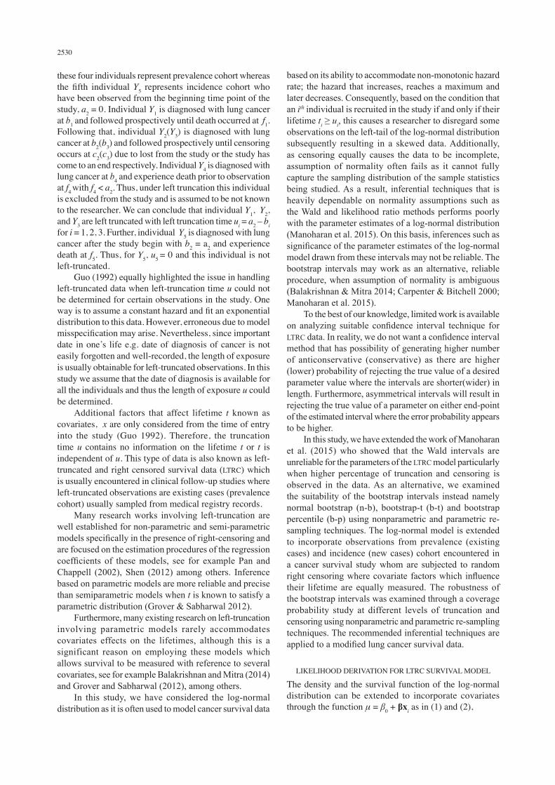
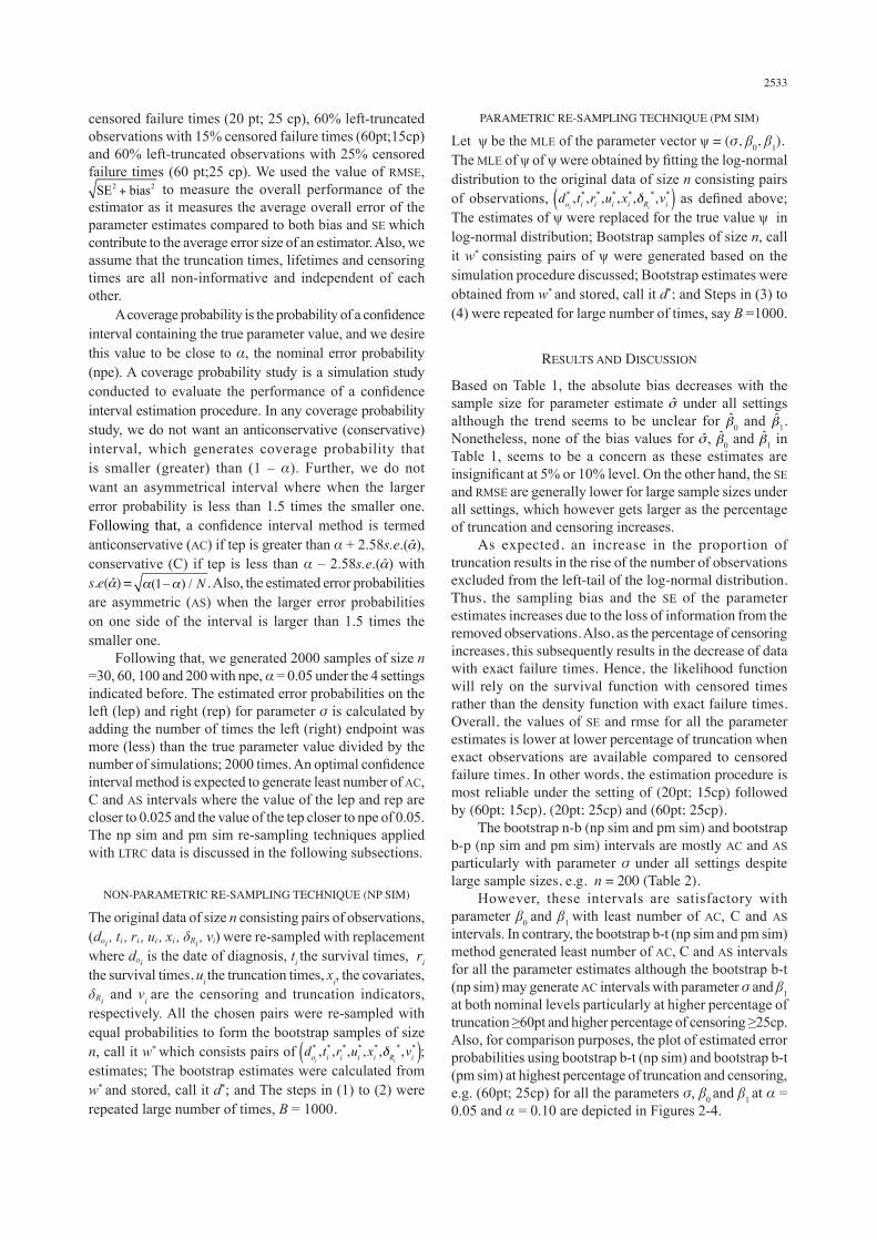
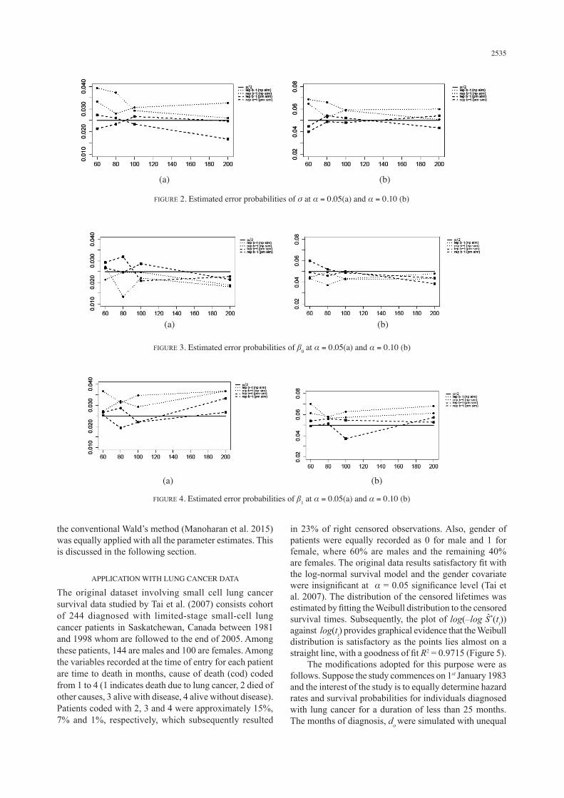
Based on Table 1, the absolute bias decreases with the sample size for parameter estimate under all settings although the trend seems to be unclear for 0 and 1. Nonetheless, none of the bias values for , 0 and 1 in Table 1, seems to be a concern as these estimates are insignificant at 5% or 10% level. On the other hand, the SE and RMSE are generally lower for large sample sizes under all settings, which however gets larger as the percentage of truncation and censoring increases. As expected, an increase in the proportion of truncation results in the rise of the number of observations excluded from the left-tail of the log-normal distribution. Thus, the sampling bias and the SE of the parameter estimates increases due to the loss of information from the removed observations. Also, as the percentage of censoring increases, this subsequently results in the decrease of data with exact failure times. Hence, the likelihood function will rely on the survival function with censored times rather than the density function with exact failure times. Overall, the values of SE and rmse for all the parameter estimates is lower at lower percentage of truncation when exact observations are available compared to censored failure times. In other words, the estimation procedure is most reliable under the setting of (20pt; 15cp) followed by (60pt; 15cp), (20pt; 25cp) and (60pt; 25cp). The bootstrap n-b (np sim and pm sim) and bootstrap b-p (np sim and pm sim) intervals are mostly AC and AS particularly with parameter σ under all settings despite large sample sizes, e.g. n = 200 (Table 2). However, these intervals are satisfactory with parameter β0 and β1 with least number of AC, C and AS intervals. In contrary, the bootstrap b-t (np sim and pm sim) method generated least number of AC, C and AS intervals for all the parameter estimates although the bootstrap b-t (np sim) may generate AC intervals with parameter σ and β1 at both nominal levels particularly at higher percentage of truncation ≥60pt and higher percentage of censoring ≥25cp. Also, for comparison purposes, the plot of estimated error probabilities using bootstrap b-t (np sim) and bootstrap b-t (pm sim) at highest percentage of truncation and censoring, e.g. (60pt; 25cp) for all the parameters σ, β0 and β1 at α = 0.05 and α = 0.10 are depicted in Figures 2-4.

2534

TABLE 2. Total number of AC, C and AS intervals using bootstrap intervals (boot) under the np and pm sim re-sampling technique with 15% and 25% censored failure times at α = 0.05

parameter σ β0 β1

setting boot sim AC C AS AC C AS AC C AS

20pt;15cp n-bb-tb-p

nppmnppmnppm

211044

000000

440044

100000

000000

000000

221020

000000

100000

60pt;15cp n-bb-tb-p

nppmnppmnppm

222043

000000

440044

000001

000000

000000

000000

000000

101000

20pt;25cp n-bb-tb-p

nppmnppmnppm

231042

000000

440044

000000

000000

000000

101011

000000

000000

60pt;25cp n-bb-tb-p

nppmnppmnppm

202044

000000

440044

000000

000000

000000

000000

000000

000000

TABLE 1. Bias, SE and rmse for parameter estimates of the LTRC model with 15% and 25% censored failure times

parameter σ β0 β1

setting n bias SE rmse bias SE rmse bias SE rmse20pt;15cp 60

80100200

-0.0131-0.0090-0.0071-0.0037

0.05160.04410.03840.0273

0.05320.04500.03910.0275

0.00180.0019-0.00060.0016

0.07050.05930.05350.0379

0.07050.05930.05350.0379

0.00110.00040.00050.0009

0.07140.06240.05340.0386

0.07140.06240.05340.0386

60pt;15cp 6080100200

-0.0132-0.0099-0.0039-0.0044

0.05220.04470.04100.0289

0.05390.04580.04120.0291

0.0029-0.0009-0.00040.0010

0.07380.06400.05620.0385

0.07390.06400.05620.0385

-0.00030.0002-0.00250.0001

0.07350.06260.05670.0401

0.07350.06260.05680.0401

20pt;25cp 6080100200

-0.0144-0.0109-0.0079-0.0035

0.05310.04720.04210.0287

0.05500.04840.04280.0289

0.00070.00110.00290.0004

0.07480.06080.05720.0397

0.07480.06080.05730.0397

-0.00390.0040-0.0014-0.0004

0.07500.06440.05630.0408

0.07510.06440.05630.0408

60pt;25cp

6080100200

-0.0133-0.0084-0.0075-0.0051

0.05560.04710.04220.0292

0.05710.04780.04290.0297

0.00030.00110.00070.0015

0.07770.06570.05780.0413

0.07770.06570.05780.0413

0.0001-0.0020-0.00150.0004

0.07630.06600.05740.0418

0.07630.06600.05740.0418

It is clear that, the estimated lep and rep using the bootstrap b-t (pm sim) are closer to α / 2 as opposed bootstrap b-t (np sim) at both nominal levels for all the parameters of the LTRC model (Figures 2-4). In other words, the resulting tep are approximately closer to either

npe, α = 0.05 or α = 0.10 at the highest percentage of truncation and censoring, 60pt; 15cp even at the highest percentage of truncation and censoring. The performance of the bootstrap b-t (pm sim) was further evaluated using a modified lung cancer data. Also, for comparison purposes,

2535

the conventional Wald’s method (Manoharan et al. 2015) was equally applied with all the parameter estimates. This is discussed in the following section.

APPLICATION WITH LUNG CANCER DATA

The original dataset involving small cell lung cancer survival data studied by Tai et al. (2007) consists cohort of 244 diagnosed with limited-stage small-cell lung cancer patients in Saskatchewan, Canada between 1981 and 1998 whom are followed to the end of 2005. Among these patients, 144 are males and 100 are females. Among the variables recorded at the time of entry for each patient are time to death in months, cause of death (cod) coded from 1 to 4 (1 indicates death due to lung cancer, 2 died of other causes, 3 alive with disease, 4 alive without disease). Patients coded with 2, 3 and 4 were approximately 15%, 7% and 1%, respectively, which subsequently resulted

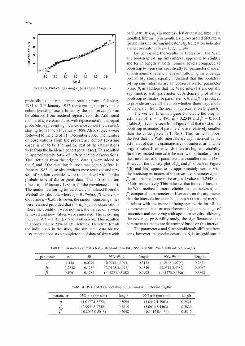
in 23% of right censored observations. Also, gender of patients were equally recorded as 0 for male and 1 for female, where 60% are males and the remaining 40% are females. The original data results satisfactory fit with the log-normal survival model and the gender covariate were insignificant at α = 0.05 significance level (Tai et al. 2007). The distribution of the censored lifetimes was estimated by fitting the Weibull distribution to the censored survival times. Subsequently, the plot of log(–log *(ti)) against log(ti) provides graphical evidence that the Weibull distribution is satisfactory as the points lies almost on a straight line, with a goodness of fit R2 = 0.9715 (Figure 5). The modifications adopted for this purpose were as follows. Suppose the study commences on 1st January 1983 and the interest of the study is to equally determine hazard rates and survival probabilities for individuals diagnosed with lung cancer for a duration of less than 25 months. The months of diagnosis, do were simulated with unequal

FIGURE 3. Estimated error probabilities of β0 at α = 0.05(a) and α = 0.10 (b)

(a) (b)

FIGURE 2. Estimated error probabilities of σ at α = 0.05(a) and α = 0.10 (b)

(a) (b)

(a) (b)

FIGURE 4. Estimated error probabilities of β1 at α = 0.05(a) and α = 0.10 (b)

2536

probabilities and replacement starting from 1st January 1981 to 31st January 1982 representing the prevalence cohort (existing cases). In reality, these observations can be obtained from medical registry records. Additional months of do were simulated with replacement and unequal probability representing the incidence cohort (new cases), starting from 1st to 31st January 1988. Also, subjects were followed to the end of 31st December 2005. The number of observations from the prevalence cohort (existing cases) is set to be 195 and the rest of the observations were from the incidence cohort (new cases). This resulted in approximately 80% of left-truncated observations. The lifetimes from the original data, ti were added to the do and if the resulting failure times occurs before 1st January 1983, these observations were removed and new sets of random variables were re-simulated with similar probabilities of the original data. The left-truncation times, ui = 1st January 1983- do for the prevalence cohort. The random censoring times, ri were simulated from the Weibull distribution, where ri ~ Weibull(λ, β) where λ = 0.005 and β = 0.50. However, the random censoring times were retained provided that ri + doi ≥ y. For observations where the condition were not met, the values of ri were removed and new values were simulated. The censoring indicator δRi = 1 if ti ≤ ri and 0 otherwise. This resulted in approximately 23% of RC lifetimes. Therefore for all the individuals in the study, the simulated data for the LTRC model consists a complete set of data of size n with

patient ID (ID), doi (in months), left-truncation time ui (in

months), lifetime ri (in months), right-censored lifetime vi (in months), censoring indicator δRi, truncation indicator vi and covariate xi for i = 1, 2, …, 244. By comparing the results in Tables 3-5, the Wald and bootstrap b-t (np sim) interval appear to be slightly shorter in length at both nominal levels compared to bootstrap b-t (pm sim) specifically for parameter σ and β1 at both nominal levels. The result following the coverage probability study equally indicated that the bootstrap b-t (np sim) intervals are anticonservative for parameter σ and β1 in addition that the Wald intervals are equally asymmetric with parameter σ. A density plot of the bootstrap estimates for parameter σ, β0 and β1 is produced to provide an overall view on whether there happens to be dispersion from the normal approximation (Figure 6). The vertical lines in Figure 5 indicate the original estimates of = 1.1480, 0 - 3.2548 and 1 = 0.1661 (Table 3). It can be seen from Figure 6(a) that most of the bootstrap estimates of parameter σ are relatively smaller than the value given in Table 3. This further support the fact that the Wald intervals are asymmetrical as the estimates of σ as the estimates are not centered around the original value. In other words, there are higher probability for the estimated interval to be narrower particularly for if the true values of the parameter σ are smaller than 1.1480. However, the density plot of β0 and β1 shown in Figure 6(b) and 6(c) appear to be approximately normal with the bootstrap estimates of the covariate parameter β0 and β1 are centered around the original value of 3.2548 and 0.1661 respectively. This indicates that intervals based on the Wald method is more reliable for parameters β0 and β1 compared to parameter σ. However, on the arguments that the intervals based on bootstrap b-t (pm sim) method is robust with the intervals being symmetric for all the parameters of the LTRC model even at higher percentage of truncation and censoring with optimum lengths following the coverage probability study, the significance of the parameter estimates are determined based on this interval. The parameter σ and β0 are significantly different from zero, however the gender covariate, β1 is insignificant at

TABLE 4. 95% and 90% bootstrap b-t (np sim) with interval lengths

parameter 95% n-b (pm sim) length 90% n-b (pm sim) lengthσβ0

β1

(1.0177,1.3272)(2.9941,3.4755)(-0.2005,0.5043)

0.30950.48140.7048

(1.0442,1.2963)(3.0636,3.4462)(-0.1412,0.4434)

0.25210.38260.5846

TABLE 3. Parameter estimates (est.), standard error (SE), 95% and 90% Wald with interval lengths

parameter est. SE 95% Wald length 90% Wald lengthσβ0

β1

1.1483.25480.1661

0.07940.12360.1784

(0.9918,1.3041)(3.0125,3.4972)(-0.1835,0.5158)

0.31230.48460.6992

(1.0168,1.2790)(3.0514,3.4582)(-0.1273,0.4596)

0.26210.40670.5868

FIGURE 5. Plot of log (-log(S*i (t )) against log(t ) )

2537

TABLE 5. 95% and 90% bootstrap b-t (pm sim) with interval lengths

parameter 95% b-t (pm sim) length 90% b-t (pm sim) lengthσβ0

β1

(1.0084,1.3408)(3.0088,3.4723)(-0.2030,0.5191)

0.33240.46340.7221

(1.0296,1.3026)(3.0557,3.4399)(-0.1327,0.4552)

0.27300.38420.5879

both nominal levels (Table 5). In other words, the effect of the gender covariate on the survival times of the small cell lung cancer patients is negligible or equally there is no statistical evidence at both nominal levels that male lung cancer patients survive longer than female lung cancer patients and vice-verse. Figure 7 depicts the plot of the survival probabilities obtained using the Kaplan-Meier and the log-normal estimator for the modified lung cancer data. It can be seen that the reduced LTRC model provides a satisfactory fit for the data as the estimated survival probabilities are approximately close to the values obtained using the non-parametric Kaplan-Meier estimator.

CONCLUSION

In conclusion, the estimation procedure generated more accurate and efficient estimates of parameters when lower truncation and censoring are present in the data. Further, based on the results from the coverage probability study, the bootstrap b-t (pm sim) provided the best alternative for all the parameters of the LTRC model as opposed to the bootstrap n-b, bootstrap b-p with least anticonservative, conservative and asymmetrical intervals. A skewed distribution of the density plot of the bootstrap estimates provided an initial insight that dependency of normality assumptions would be erroneous specifically for the shape parameter σ of the LTRC model. Thus, Wald intervals which heavily dependable on normality assumptions are not recommended as the inference based on these confidence interval estimates would be bias and unreliable. In such cases, parametric bootstrap intervals are highly recommended as these intervals but are based on distribution of data in hand which subsequently relaxes the assumption of normality, robust against higher percentage of truncation and censoring present in the data and convenient as it worked well with all the parameters of the LTRC model. The proposed bootstrap b-t (pm sim) is equally applicable with parameters from similar log-location scale models as the log-logistic distribution or when the assumption of normality is ambiguous.

FIGURE 6. Density plot of the bootstrap estimates for parameter σ (a), β0 and β1 (c)

(a) (b)

(c)

FIGURE 7. Plot of estimated survival probabilities from the fitted distribution (solid line) and Kaplan- Meier estimator (dotted lines)

2538

ACKNOWLEDGEMENTS

This work was supported by the Fundamental Research Grant Scheme (FRGS), VOT 5524226, University Putra Malaysia. We would like to equally extend our gratitude to Dr. Patricia Tai from University of Saskatchewan, Saskatoon, Canada for providing the data.

REFERENCES

Arasan, J. & Lunn, M. 2008. Alternative interval estimation for parameters of bivariate exponential model with time varying covariate. Computational Statistics 23(4): 605-622.

Balakrishnan, N. & Mitra, D. 2014. Some further issues concerning likelihood inference for left truncated and right censored lognormal data. Communications in Statistics: Simulation and Computation 43(2): 400-416.

Carpenter, J. & Bithell, J. 2000. Bootstrap confidence intervals: When, which, what? A practical guide for medical statisticians for parameters of bivariate exponential model with time varying covariate. Statistics in Medicine 19(9): 1141-1164.

Efron, B. 1981. Censored data and the bootstrap. Journal of the American Statistical Association 76(374): 312-319.

Gross, S.T. & Lai, T.L. 1996. Nonparametric estimation and regression analysis with left-truncated and right-censored data. Journal of the American Statistical Association 91(435): 1166-1180.

Grover, G. & Sabharwal, A. 2012. A parametric approach to estimate survival time of diabetic nephoropathy with left-truncated and right censored data. International Journal of Statistics and Probability 1(1): 128-137.

Guo, G. 1992. Event-history analysis for left-truncated data. Sociological Methodology 23(1): 217-243.

Hjort, N.L. 1992. On inference in parametric survival data models. International Statistical Review/Revue Internationale de Statistique 60(3): 355-387.

Manoharan, T., Arasan, J., Midi, H. & Adam, M.B. 2015. A coverage probability on the parameters of the log-normal distribution in the presence of left-truncated and right-censored survival data. Malaysian Journal of Mathematical Sciences 9(1): 127-144.

Pan, W. & Chappell, R. 2002. Estimation in the cox proportional hazards model with left-truncated and interval-censored data. Biometrics 58(1): 64-70.

Robinson, J. 1983. Bootstrap confidence intervals in location-scale models with progressive censoring. Technometrics 25(2): 179-817.

Shen, P.S. 2012. Proportional hazards regression with interval-censored and left-truncated data. Journal of Statistical Computation and Simulation 84(2): 1-9.

Tai, P., Chapman, J.A.W., Yu, E., Jones, D., Yu, C., Yuan, F. & Sang-Joon, L. 2007. Disease specific survival for limited-stage small-cell lung cancer affected by statistical method of assessment. BMC Cancer 7(1): 31-39.

Wang, M.C. 1991. Nonparametric estimation from cross-sectional survival data. Journal of the American Statistical Association 86(413): 13-143.

Department of Mathematics, Faculty of ScienceUniversiti Putra Malaysia43400 UPM Serdang, Selangor Darul EhsanMalaysia

Laboratory of Computational Statistics and Operations ResearchUniversiti Putra Malaysia43400 UPM Serdang, Selangor Darul EhsanMalaysia

*Corresponding author; email: mthirunanthini@gmail.com

Received: 29 March 2016Accepted: 18 April 2017

2539

APPENDIX