Bootstrap Inference in Econometrics

by

James G. MacKinnon

Department of EconomicsQueen’s University

Kingston, Ontario, CanadaK7L 3N6

jgm@qed.econ.queensu.ca

Abstract

The astonishing increase in computer performance over the past two decades has made itpossible for economists to base many statistical inferences on simulated, or bootstrap,distributions rather than on distributions obtained from asymptotic theory. In thispaper, I review some of the basic ideas of bootstrap inference. The paper discussesMonte Carlo tests, several types of bootstrap test, and bootstrap confidence intervals.Although bootstrapping often works well, it does not do so in every case.

Revised June, 2002

This paper was presented as the Presidential Address at the 2002 Annual Meeting of theCanadian Economics Association. This research was supported, in part, by two grantsfrom the Social Sciences and Humanities Research Council of Canada. I am grateful toRussell Davidson, Dwayne Benjamin, and John Galbraith for comments.

1. Introduction

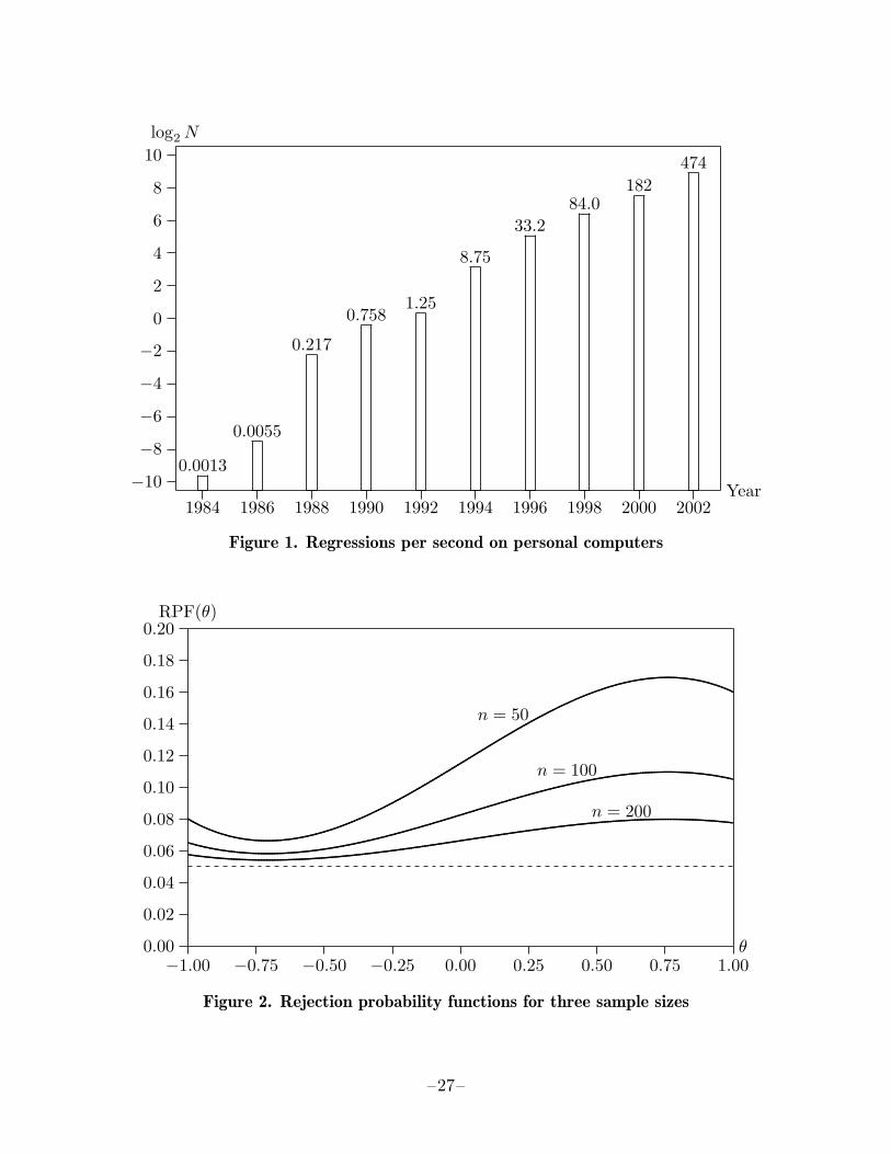
One of the most remarkable examples of technological progress has been the massiveincrease in the speed of digital computers during the past forty years. For scientificcomputing, a typical personal computer of today is several hundred times as fast as atypical PC of just a decade ago, although it costs less than half as much. Even thePC of a decade ago was faster than multi-million dollar mainframe computers of justtwo decades ago. Some of this progress is documented in Figure 1, which shows thenumber of medium-sized ordinary least squares regressions (4000 observations and 20regressors) that a more or less state-of-the-art, but affordable, personal computer couldperform in a single second at various points in time over the past two decades.1

Since computer time is now very cheap, it makes sense for applied econometricians touse far more of it than they did just a few years ago. There are at least three waysin which they have been doing so. One approach is to estimate very ambitious, struc-tural models, which often involve explicitly modeling choice at the level of individualagents. For many of these models, simulations are needed simply to estimate the model.Because this is very time-consuming, inference is normally based on standard asymp-totic results. Important early examples of this approach include Pakes (1986) and Rust(1987). Eckstein and Wolpin (1989) and Stern (1997) provide useful surveys.

A second line of research involves Bayesian estimation using Markov-chain Monte Carlomethods; see, among many others, Albert and Chib (1993), McCulloch and Rossi (1994),Geweke (1999), and Elerian, Chib, and Shephard (2001). With this approach, inferenceis exact, in the Bayesian sense, but it generally depends upon strong distributionalassumptions and the investigator’s prior beliefs.

The third line of research, which is the one I will discuss here, is to base statisticalinferences on distributions that are calculated by simulation rather than on ones thatare suggested by asymptotic theory and are strictly valid only when the sample size isinfinitely large. In this approach, parameter estimates and test statistics are calculatedin fairly conventional ways, but P values and confidence intervals are computed using“bootstrap” distributions obtained by simulation. This bootstrap approach can often,but does not always, lead to much more accurate inferences than traditional approachesare capable of. However, like every tool in econometrics, it must be used with care.

The reason for using bootstrap inference is that hypothesis tests and confidence intervalsbased on asymptotic theory can be seriously misleading when the sample size is not large.There are many examples. One is the popular J test of nonnested regression models(Davidson and MacKinnon, 1981), which always rejects the null hypothesis too often.In extreme cases, even for sample sizes as large as 50, an asymptotic J test at the .05level can reject a true null hypothesis more than 80% of the time; see Davidson andMacKinnon (2002a). Some versions of the information matrix test overreject even moreseverely. Davidson and MacKinnon (1992) report a simulation in which one such test

1 The numbers in Figure 1 are based on my own Fortran programs run on various machines that Ihave had access to. Times are for an XT clone (1984), a 286/10 (1986), a 386/20 (1988), a 486/25(1990), a 486DX2/50 (1992), a Pentium 90 (1994), a Pentium Pro 200 (1996), a Pentium II/450(1998), an Athlon 800 (2000), and a Pentium 4/2200 (2002).

–1–

at the .05 level rejected a true null hypothesis an astounding 99.9% of the time whenthe sample size was 200.

Of course, asymptotic tests are not always misleading. In many cases, a bootstrap testwill yield essentially the same inferences as an asymptotic test based on the same teststatistic. Although this does not necessarily imply that the asymptotic test is reliable,the investigator may reasonably feel greater confidence in the results of asymptotic teststhat have been confirmed in this way.

Statistical inference in a classical framework involves either testing hypotheses or con-structing confidence intervals. Most of this paper will focus on hypothesis testing,because simulation-based hypothesis testing is generally easier and more reliable thanconstructing simulation-based confidence intervals. Moreover, hypothesis tests and con-fidence intervals are very closely related, so that much of what is said about bootstraptests will also be applicable to bootstrap confidence intervals.

The next section discusses Monte Carlo tests, which can be thought of as a special caseof bootstrap tests. Section 3 then goes on to discuss bootstrap tests more generally.Section 4 explains why bootstrap tests will often work well and provides evidence from asimulation experiment for a case in which they work extremely well. Section 5 considersthree common situations in which bootstrap tests do not always work well and providesevidence from several simulation experiments which illustrates the problems that canarise. Section 6 deals with the power of bootstrap tests. Finally, Section 7 brieflydiscusses bootstrap confidence intervals.

2. Monte Carlo Tests

Statisticians generally make a distinction between two types of simulation-based tests,namely, Monte Carlo tests and bootstrap tests. In this section, I will begin by discussinga fairly simple example of a Monte Carlo test. In the next section, I will move on to adiscussion of bootstrap tests.

One of the best-known test statistics in econometrics is the d statistic proposed byDurbin and Watson (1950, 1951) for testing the null hypothesis that the error terms ofa linear regression model are serially uncorrelated. The model under test is

yt = Xtβ + ut, ut ∼ NID(0, σ2), (1)

where there are n observations, and the row vector of regressors Xt is treated as fixed.If ut denotes the tth residual from OLS estimation of (1), then the Durbin-Watsonstatistic is

d =

∑nt=2(ut − ut−1)2∑n

t=1 u2t

. (2)

The finite-sample distribution of d depends on X, the matrix of regressors with tth rowXt. Therefore, it is customary to base inferences on tables which merely provide boundson the critical values. Since these bounds are often quite far apart, it is frequentlyimpossible to tell whether the null hypothesis of serial independence should be rejected.The exact distribution of d can be calculated, but very few econometric packages do so.

–2–

Under the null hypothesis, the vector of OLS residuals is

u = MXu, where MX ≡ I−X(X>X)−1X>.

Thus the residuals depend solely on the error terms and the matrix X. Since they areevidently proportional to σ, we can see from (2) that the statistic d depends only onthe normalized error terms εt ≡ ut/σ and the matrix X. It does not depend on β or σ2

at all. A statistic like d that does not depend on any unknown parameters is said to bepivotal. For any pivotal statistic, we can perform an exact simulation-based test. Sucha test is called a Monte Carlo test. When we say that the test is exact, we mean thatthe probability of rejecting the null hypothesis when it is true is precisely equal to α,the nominal level of the test, which would often be .10, .05, or .01.

The steps required to perform a Monte Carlo test based on the Durbin-Watson statisticare as follows:

1. Estimate the linear regression model (1) and compute d.

2. Choose B, the number of simulations. It should be chosen so that α(B + 1) is aninteger for all levels α of interest. A common choice is B = 999. However, sinceestimating a linear regression model and computing d is very inexpensive, B = 9999might be a slightly better choice. It is also possible to start with a small value like99 and then increase it if the outcome of the test is not clear.

3. Generate B simulated samples, or bootstrap samples, indexed by j, by drawingvectors of errors u∗j from the standard normal distribution. Then regress them onX to generate B simulated residual vectors u∗j .

4. For each bootstrap sample, compute d∗j from the bootstrap residuals u∗j using theformula (2).

5. Use d and the d∗j to compute a P value. The Durbin-Watson statistic is often treatedas a one-tailed test against positive serial correlation, and the null hypothesis isrejected whenever d is sufficiently small. For such a test, the simulated P value is

p∗(d) =1B

B∑

j=1

I(d∗j ≤ d).

Here I(·) denotes the indicator function, which is equal to 1 if its argument is trueand 0 otherwise. Thus the simulated P value is the fraction of the time that d∗j issmaller than d. Alternatively, we could test against negative serial correlation bycalculating the fraction of the time that d∗j is larger than d.

6. Reject the null hypothesis that the error terms are serially independent if whicheversimulated P value is appropriate is less than α, the level of the test. To test for bothpositive and negative serial correlation, we could reject whenever the simulated Pvalue for either one-tailed test is less than α/2.

The simulated P value p∗(d) makes sense intuitively. If a substantial proportion of thed∗j are more extreme than d, then the probability of obtaining a test statistic as or more

–3–

extreme than d must be high, the simulated P value will be large, and we will not rejectthe null hypothesis that the error terms are serially uncorrelated. Conversely, if veryfew of the d∗j are more extreme than d, then the probability of obtaining a test statisticas or more extreme than d must be low, the simulated P value will be small, and wewill reject the null hypothesis.

Because d is pivotal, this procedure yields an exact test. Suppose, for concreteness, thatB = 99 and α = .05. Then there are 100 possible values that p∗(d) can take on: 0,1/99, 2/99, . . . , 98/99, 1. If the null hypothesis is true, d and the d∗j come from exactlythe same distribution. Therefore, every possible value of p∗(d) has exactly the sameprobability, namely, 1/100. There are five values that will cause us to reject the null:0, 1/99, 2/99, 3/99, and 4/99. Under the null hypothesis, the probability that one ofthese five values will occur by chance is precisely .05. Note that this argument wouldnot work if α(B + 1) were not an integer.

Simulation necessarily introduces randomness into our test procedure, and it seems clearthat this must have a cost. In this case, the cost is a loss of power. A test based on99 simulations will be less powerful than a test based on B = 999, which in turn willbe less powerful than one based on B = 9999, and so on. However, as we will see inSection 6, the power loss is generally very small indeed when B ≥ 999.

As I remarked above, it is possible to start with a small value of B, say B = 99, and thenperform more replications only if the initial results are ambiguous. If, for example, 38out of the first 99 bootstrap samples yield test statistics more extreme than the actualone, then we can be confident that the null hypothesis is not rejected at any standardsignificance level, and there is no need to generate any more bootstrap samples. If theinitial results are not so clear, we can generate more bootstrap samples until we obtain asufficiently accurate estimate of the P value. Davidson and MacKinnon (2000) proposea formal procedure for doing this.

Procedures very similar to the one just described for the Durbin-Watson test can alsobe used to perform a variety of other Monte Carlo tests of linear regression models withfixed regressors and error terms that follow a distribution known up to scale, whichdoes not have to be the normal distribution. These include tests for higher-order serialcorrelation based on the Gauss-Newton regression, tests for heteroskedasticity, tests forskewness and kurtosis, and tests of certain types of linear restrictions in multivariatelinear regression models. As long as the test statistic simply depends on error termswith a known distribution and fixed regressors, it will be pivotal, and we can performan exact simulation-based test. Monte Carlo tests were first proposed by Dwass (1957).For a much fuller discussion of these tests, see Dufour and Khalaf (2001).

3. Bootstrap Tests

When a test statistic is not pivotal, we cannot use a Monte Carlo test. However, we canuse bootstrap tests that work in very much the same way. For example, the Durbin-Watson d statistic would no longer be pivotal if the distribution of the error terms wereunknown. But we can still generate bootstrap samples (in a somewhat different way),compute the d∗j , and calculate bootstrap P values exactly as before. These bootstrap

–4–

P values will not be entirely accurate, but they will often be much more accurate thanP values calculated from an asymptotic distribution.

Without the normality assumption, it does not make sense to generate bootstrap errorsfrom the normal distribution. Instead, we want to generate them nonparametrically.One of the simplest and most popular approaches is to obtain the u∗j by resampling theresiduals ut. To generate a single bootstrap sample, we pick n integers between 1 and nat random with equal probability. If the tth integer is equal to k, we set u∗t = uk. In thisway, we effectively generate the bootstrap error terms from the empirical distributionfunction of the residuals. Resampling is the key idea of the bootstrap as it was originallyproposed by Efron (1982).

As every student of econometrics knows, OLS residuals have smaller variance than theerror terms on which they are based. Thus it would seem to be desirable to resamplenot the vector u of raw residuals but rather the vector of rescaled residuals

u ≡(

n

n− k

)1/2

u, (3)

the elements of which have variance σ2. In the case of the Durbin-Watson statistic andother test statistics that do not depend on σ2, it makes absolutely no difference whetheror not the residuals have been rescaled before we resample them. However, for manyother test statistics, it is important to resample u instead of u.

Other, more complicated, methods of rescaling the residuals can also be used. Forexample, we could resample the vector with typical element

ut =(

n

n− 1

)1/2(

ut

(1− ht)1/2− 1−

n

n∑s=1

us

(1− hs)1/2

), (4)

where ht denotes the tth diagonal element of the hat matrix, that is, the matrix PX ≡I−MX . In expression (4), we divide by (1− ht)1/2 in order to ensure that, if the errorterms were homoskedastic, all the transformed residuals would have the same variance.We then subtract the mean of the residuals after the initial transformation so that thetransformed residuals will have mean zero, and we then multiply by the square root ofn/(n− 1) to undo the shrinkage caused by subtracting the mean.

In many cases, the unrestricted model is also a regression model, and we could resamplethe residuals for that model instead of the residuals for the restricted model. Indeed,several authors, including van Giersbergen and Kiviet (2002), have advocated doingprecisely this, on the grounds that it will improve power. The argument is that, whenthe null is false, the unrestricted residuals will provide a better approximation to thedistribution of the error terms. As we will see in Section 6, this conjecture appears tobe false.

Bootstrap tests based on nonpivotal test statistics are calculated in essentially the sameway as Monte Carlo tests. We first calculate a test statistic, say τ , in the usual way.Possibly as a byproduct of doing so, we estimate the model under the null hypothesis and

–5–

obtain estimates of all the quantities needed to generate bootstrap samples that satisfythe null hypothesis. The data-generating process used to generate these samples iscalled the bootstrap DGP. The bootstrap DGP may be purely parametric, but it ofteninvolves some sort of resampling so as to avoid making distributional assumptions.It must always satisfy the null hypothesis. We then generate B bootstrap samples,compute a bootstrap test statistic τ∗j using each of them, and calculate the bootstrapP value p∗(τ) as the proportion of the τ∗j that are more extreme than τ . If p∗(τ) is lessthan α, we reject the null hypothesis.

Instead of calculating a P value, some authors prefer to calculate a bootstrap criticalvalue based on the τ∗j and reject the null hypothesis whenever τ exceeds it. If the test isone for which we reject when τ is large, then the bootstrap critical value c∗α is the 1−αquantile of the τ∗j . When α(B +1) is an integer, this is simply number (1−α)(B +1) inthe list of the τ∗j , sorted from smallest to largest. For example, if B = 999 and α = .05,then c∗α is number 950 in the sorted list.

Rejecting the null hypothesis whenever τ exceeds c∗α will yield exactly the same resultsas rejecting whenever the bootstrap P value is less than α. However, since it does notyield a P value, it normally provides less information. But calculating critical valuesmay be desirable when B is small (because the test is expensive to compute) and τ ismore extreme than all of the τ∗j . In such a case, observing that τ greatly exceeds theestimated critical value may give us more confidence that the null is false than merelyseeing that p∗(τ) is equal to 0.

4. When Do Bootstrap Tests Perform Well?

The reason for using bootstrap tests instead of asymptotic tests is that we hope to makefewer mistakes by doing so. Many asymptotic tests overreject in finite samples, oftenvery severely. Other asymptotic tests underreject, sometimes quite seriously. By usinga bootstrap test instead of an asymptotic one, we can usually, but not always, makemore accurate inferences. Ideally, a test will have a small error in rejection probability,or ERP. This is the difference between the actual rejection frequency under the nullhypothesis and the level of the test. The ERP of a bootstrap test is usually, but notalways, smaller than the ERP of the asymptotic test on which it is based. In manycases, it is a great deal smaller.

The theoretical literature on the finite-sample performance of bootstrap tests, such asBeran (1988) and Hall and Titterington (1989), is primarily concerned with the rateat which the ERP of bootstrap tests declines as the sample size increases. It has beenshown that, in a variety of circumstances, the ERP of bootstrap tests declines morerapidly than the ERP of the corresponding asymptotic test. The essential requirementis that the underlying test statistic be asymptotically pivotal. This is a much weakercondition than that the statistic be pivotal. It means that, as the sample size tends toinfinity, any dependence of the distribution on unknown parameters or other unknownfeatures of the data-generating process must vanish. Of course, any test statistic thathas a known asymptotic distribution which is free of nuisance parameters, as do thevast majority of test statistics in econometrics, must be asymptotically pivotal.

–6–

It is not hard to see intuitively why the ERP of a bootstrap test based on an asymp-totically pivotal test statistic will decline more rapidly than the ERP of an asymptotictest based on the same test statistic. Suppose, for simplicity, that the finite-sampledistribution of a test statistic τ depends on just one nuisance parameter, say θ. Thenwe can graph the rejection probability of the asymptotic test as a function of θ, as inFigure 2. If the rejection probability function, or RPF, is flat, then τ is pivotal, andthe bootstrap test will work perfectly. If it is not flat, then the bootstrap test will notwork perfectly, because the distribution of the τ∗j , which is based on an estimate θ, willdiffer from the distribution of τ , which is based on the unknown true value θ0.

As Davidson and MacKinnon (1999a) showed, the ERP of a bootstrap test depends onthe slope of the RPF, but only if θ is biased, and on its curvature, whether or not θ isbiased. Whenever τ is asymptotically pivotal, the RPF must converge to a horizontalline as the sample size tends to infinity. This is illustrated in Figure 2, which showsRPFs for the same test for three different sample sizes. The fact that the slope andcurvature of the RPF become smaller as the sample size increases would, by itself, causethe ERP of the bootstrap test to decrease at the same rate as the ERP of the asymptotictest. But increasing the sample size also causes both the bias and the variance of θ todecrease. This further reduces the ERP of the bootstrap test, but it has no effect onthe ERP of the asymptotic test. Therefore, as the sample size increases, the ERP of abootstrap test should improve more rapidly than that of an asymptotic test based onthe same test statistic.

This result does not imply that a bootstrap test will always outperform the correspond-ing asymptotic test. There may well be values of θ for which the latter happens toperform extremely well and the bootstrap test performs less well. However, if the ERPof an asymptotic test is large, then it is increasingly likely, as the sample size increases,that the ERP of a bootstrap test based on it will be smaller. In practice, it often seemsto be very much smaller. Thus, by using bootstrap tests, we may be able to avoid thegross errors of inference that frequently occur when we act as if test statistics actuallyfollow their asymptotic distributions.

Let us now consider a specific example which illustrates the relationship between asymp-totic and bootstrap tests. When a regression model includes lagged dependent variables,the Durbin-Watson statistic is not valid. In this situation, one popular way of testingfor first-order serial correlation, which was suggested by Durbin (1970) and Godfrey(1978), is to run the original regression again with the lagged OLS residuals added asan additional regressor. The t statistic on the lagged residuals, which we will refer toas the Durbin-Godfrey statistic, can be used to perform an asymptotically valid test forfirst-order serial correlation; see Davidson and MacKinnon (1993, Chapter 10).

The finite-sample distribution of the Durbin-Godfrey statistic depends on the samplesize, the matrix of regressors, and the values of all the parameters. The parameter onthe lagged dependent variable is particularly important. For purposes of illustration, Igenerated data from the model

yt = β1 +4∑

j=2

βjXtj + δyt−1 + ut, ut ∼ N(0, σ2), (5)

–7–

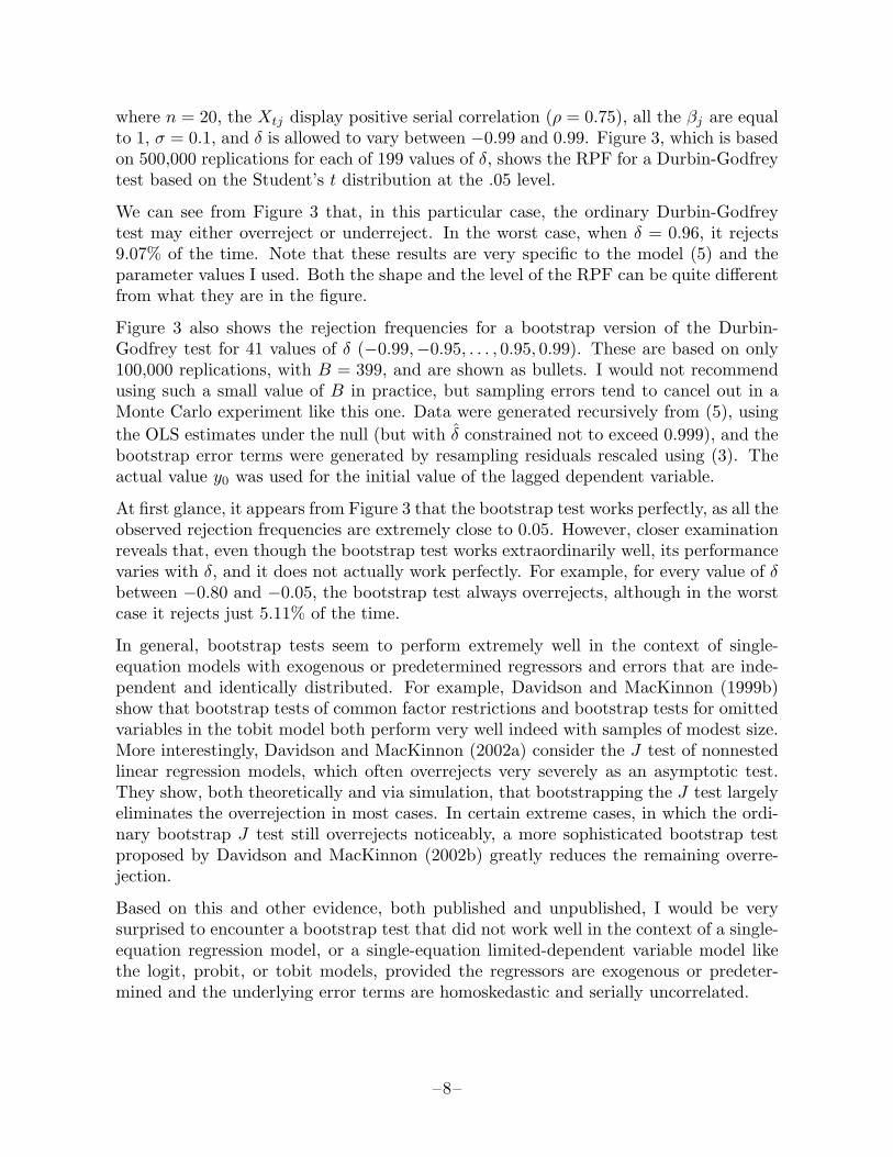
where n = 20, the Xtj display positive serial correlation (ρ = 0.75), all the βj are equalto 1, σ = 0.1, and δ is allowed to vary between −0.99 and 0.99. Figure 3, which is basedon 500,000 replications for each of 199 values of δ, shows the RPF for a Durbin-Godfreytest based on the Student’s t distribution at the .05 level.

We can see from Figure 3 that, in this particular case, the ordinary Durbin-Godfreytest may either overreject or underreject. In the worst case, when δ = 0.96, it rejects9.07% of the time. Note that these results are very specific to the model (5) and theparameter values I used. Both the shape and the level of the RPF can be quite differentfrom what they are in the figure.

Figure 3 also shows the rejection frequencies for a bootstrap version of the Durbin-Godfrey test for 41 values of δ (−0.99,−0.95, . . . , 0.95, 0.99). These are based on only100,000 replications, with B = 399, and are shown as bullets. I would not recommendusing such a small value of B in practice, but sampling errors tend to cancel out in aMonte Carlo experiment like this one. Data were generated recursively from (5), usingthe OLS estimates under the null (but with δ constrained not to exceed 0.999), and thebootstrap error terms were generated by resampling residuals rescaled using (3). Theactual value y0 was used for the initial value of the lagged dependent variable.

At first glance, it appears from Figure 3 that the bootstrap test works perfectly, as all theobserved rejection frequencies are extremely close to 0.05. However, closer examinationreveals that, even though the bootstrap test works extraordinarily well, its performancevaries with δ, and it does not actually work perfectly. For example, for every value of δbetween −0.80 and −0.05, the bootstrap test always overrejects, although in the worstcase it rejects just 5.11% of the time.

In general, bootstrap tests seem to perform extremely well in the context of single-equation models with exogenous or predetermined regressors and errors that are inde-pendent and identically distributed. For example, Davidson and MacKinnon (1999b)show that bootstrap tests of common factor restrictions and bootstrap tests for omittedvariables in the tobit model both perform very well indeed with samples of modest size.More interestingly, Davidson and MacKinnon (2002a) consider the J test of nonnestedlinear regression models, which often overrejects very severely as an asymptotic test.They show, both theoretically and via simulation, that bootstrapping the J test largelyeliminates the overrejection in most cases. In certain extreme cases, in which the ordi-nary bootstrap J test still overrejects noticeably, a more sophisticated bootstrap testproposed by Davidson and MacKinnon (2002b) greatly reduces the remaining overre-jection.

Based on this and other evidence, both published and unpublished, I would be verysurprised to encounter a bootstrap test that did not work well in the context of a single-equation regression model, or a single-equation limited-dependent variable model likethe logit, probit, or tobit models, provided the regressors are exogenous or predeter-mined and the underlying error terms are homoskedastic and serially uncorrelated.

–8–

5. When Do Bootstrap Tests Perform Badly?

As the qualifications at the end of the preceding paragraph suggest, there are at leastthree situations in which bootstrap tests cannot be relied upon to perform particularlywell. I briefly discuss each of these in this section.

5.1 Models with Serial Correlation

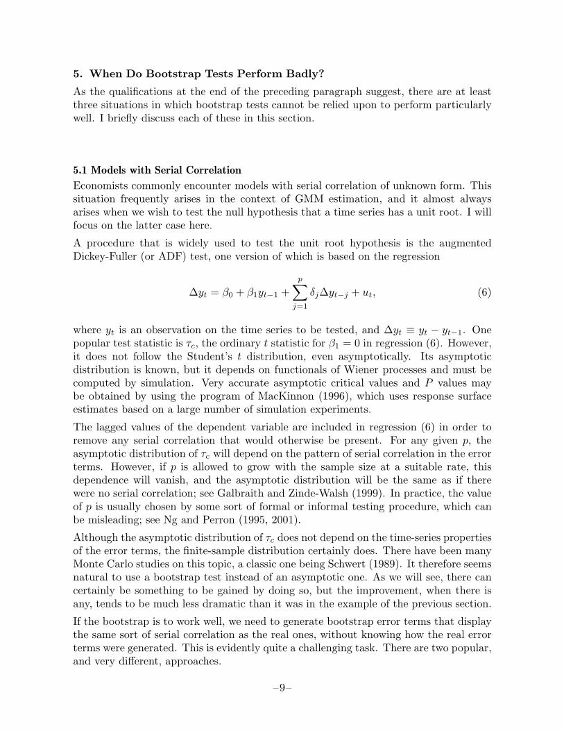
Economists commonly encounter models with serial correlation of unknown form. Thissituation frequently arises in the context of GMM estimation, and it almost alwaysarises when we wish to test the null hypothesis that a time series has a unit root. I willfocus on the latter case here.

A procedure that is widely used to test the unit root hypothesis is the augmentedDickey-Fuller (or ADF) test, one version of which is based on the regression

∆yt = β0 + β1yt−1 +p∑

j=1

δj∆yt−j + ut, (6)

where yt is an observation on the time series to be tested, and ∆yt ≡ yt − yt−1. Onepopular test statistic is τc, the ordinary t statistic for β1 = 0 in regression (6). However,it does not follow the Student’s t distribution, even asymptotically. Its asymptoticdistribution is known, but it depends on functionals of Wiener processes and must becomputed by simulation. Very accurate asymptotic critical values and P values maybe obtained by using the program of MacKinnon (1996), which uses response surfaceestimates based on a large number of simulation experiments.

The lagged values of the dependent variable are included in regression (6) in order toremove any serial correlation that would otherwise be present. For any given p, theasymptotic distribution of τc will depend on the pattern of serial correlation in the errorterms. However, if p is allowed to grow with the sample size at a suitable rate, thisdependence will vanish, and the asymptotic distribution will be the same as if therewere no serial correlation; see Galbraith and Zinde-Walsh (1999). In practice, the valueof p is usually chosen by some sort of formal or informal testing procedure, which canbe misleading; see Ng and Perron (1995, 2001).

Although the asymptotic distribution of τc does not depend on the time-series propertiesof the error terms, the finite-sample distribution certainly does. There have been manyMonte Carlo studies on this topic, a classic one being Schwert (1989). It therefore seemsnatural to use a bootstrap test instead of an asymptotic one. As we will see, there cancertainly be something to be gained by doing so, but the improvement, when there isany, tends to be much less dramatic than it was in the example of the previous section.

If the bootstrap is to work well, we need to generate bootstrap error terms that displaythe same sort of serial correlation as the real ones, without knowing how the real errorterms were generated. This is evidently quite a challenging task. There are two popular,and very different, approaches.

–9–

The first approach, which is semiparametric, is called the sieve bootstrap. We firstimpose the unit root null and estimate an autoregressive model of order p, where p ischosen in a way that allows it to increase with the sample size. We then generate sim-ulated innovations by resampling the rescaled residuals from the autoregressive model.The serially correlated bootstrap error terms are then constructed from the model andthe innovations. For details, see Buhlmann (1997, 1998), Choi and Hall (2000), Park(2002), and Chang and Park (2002). Although it has merit, this approach is not entirelysatisfactory. For samples of moderate size, the AR(p) approximation may not be a goodone. Even if it is, the parameter estimates are certain to be biased. Thus it is likelythat the bootstrap samples will differ from the real one in important respects.

The second approach, which is fully nonparametric, is to resample groups of residuals.Conceptually, one of the simplest such methods is the block bootstrap, which has beenproposed in various forms by Carlstein (1986), Kunsch (1989), Politis and Romano(1994), and a number of other authors. One particular block bootstrap procedureworks as follows:

• Pick a block length b < n.

• Form n blocks of b residuals, each starting with a different one of the n residuals,and (in this version) wrapping around to the beginning if necessary.

• Generate the bootstrap errors by resampling the blocks. If n/b is an integer, therewill be n/b blocks. Otherwise, the last block will have to be shorter than b.

Numerous other block bootstrap procedures exist, some of which have better theoreticalproperties than others; see Lahiri (1999). Although the one just described is probablyas good as any, it is far from satisfactory. The blocks of residuals will not have the sameproperties as the underlying error terms, and the patterns of dependence within eachblock will be broken between each block and where the blocks wrap around. Neverthe-less, it can be shown that, if b is allowed to tend to infinity at the correct rate, whichis slower than the rate at which n does so, the bootstrap samples will have the rightproperties asymptotically.

To illustrate these two approaches, I have undertaken a few Monte Carlo experimentsthat examine the performance of the ADF test based on regression (6), with p = 4, ina very special case. The data were generated by

∆yt = ut, ut = ρut−1 + εt, εt ∼ N(0, 1), (7)

in which the error terms follow an AR(1) process with parameter ρ. The parametersβ0 and β1 that appear in (6) do not appear here, because they are both equal to 0under the null hypothesis of a unit root. In all the experiments, there were n = 100observations.

Figure 4 shows rejection frequencies at the .05 level as a function of ρ for four differenttests. The solid line, which is based on one million replications for each of 199 equally-spaced values of ρ between −0.99 and 0.99, shows the rejection frequencies for the usualADF test based on the critical value −2.8906, which is what the program of MacKinnon(1996) gives for a sample of size 100. The various symbols show rejection frequencies

–10–

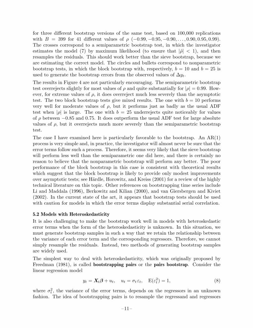
for three different bootstrap versions of the same test, based on 100,000 replicationswith B = 399 for 41 different values of ρ (−0.99,−0.95,−0.90, . . . , 0.90, 0.95, 0.99).The crosses correspond to a semiparametric bootstrap test, in which the investigatorestimates the model (7) by maximum likelihood (to ensure that |ρ| < 1), and thenresamples the residuals. This should work better than the sieve bootstrap, because weare estimating the correct model. The circles and bullets correspond to nonparametricbootstrap tests, in which the block bootstrap with, respectively, b = 10 and b = 25 isused to generate the bootstrap errors from the observed values of ∆yt.

The results in Figure 4 are not particularly encouraging. The semiparametric bootstraptest overrejects slightly for most values of ρ and quite substantially for |ρ| = 0.99. How-ever, for extreme values of ρ, it does overreject much less severely than the asymptotictest. The two block bootstrap tests give mixed results. The one with b = 10 performsvery well for moderate values of ρ, but it performs just as badly as the usual ADFtest when |ρ| is large. The one with b = 25 underrejects quite noticeably for valuesof ρ between −0.85 and 0.75. It does outperform the usual ADF test for large absolutevalues of ρ, but it overrejects much more severely than the semiparametric bootstraptest.

The case I have examined here is particularly favorable to the bootstrap. An AR(1)process is very simple and, in practice, the investigator will almost never be sure that theerror terms follow such a process. Therefore, it seems very likely that the sieve bootstrapwill perform less well than the semiparametric one did here, and there is certainly noreason to believe that the nonparametric bootstrap will perform any better. The poorperformance of the block bootstrap in this case is consistent with theoretical resultswhich suggest that the block bootstrap is likely to provide only modest improvementsover asymptotic tests; see Hardle, Horowitz, and Kreiss (2001) for a review of the highlytechnical literature on this topic. Other references on bootstrapping time series includeLi and Maddala (1996), Berkowitz and Kilian (2000), and van Giersbergen and Kiviet(2002). In the current state of the art, it appears that bootstrap tests should be usedwith caution for models in which the error terms display substantial serial correlation.

5.2 Models with Heteroskedasticity

It is also challenging to make the bootstrap work well in models with heteroskedasticerror terms when the form of the heteroskedasticity is unknown. In this situation, wemust generate bootstrap samples in such a way that we retain the relationship betweenthe variance of each error term and the corresponding regressors. Therefore, we cannotsimply resample the residuals. Instead, two methods of generating bootstrap samplesare widely used.

The simplest way to deal with heteroskedasticity, which was originally proposed byFreedman (1981), is called bootstrapping pairs or the pairs bootstrap. Consider thelinear regression model

yt = Xtβ + ut, ut = σtεt, E(ε2t ) = 1, (8)

where σ2t , the variance of the error terms, depends on the regressors in an unknown

fashion. The idea of bootstrapping pairs is to resample the regressand and regressors

–11–

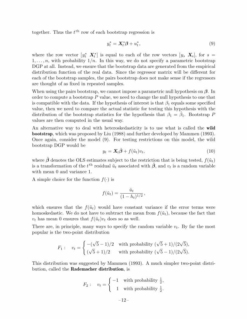
together. Thus the tth row of each bootstrap regression is

y∗t = X∗t β + u∗t , (9)

where the row vector [y∗t X∗t ] is equal to each of the row vectors [ys Xs], for s =

1, . . . , n, with probability 1/n. In this way, we do not specify a parametric bootstrapDGP at all. Instead, we ensure that the bootstrap data are generated from the empiricaldistribution function of the real data. Since the regressor matrix will be different foreach of the bootstrap samples, the pairs bootstrap does not make sense if the regressorsare thought of as fixed in repeated samples.

When using the pairs bootstrap, we cannot impose a parametric null hypothesis on β. Inorder to compute a bootstrap P value, we need to change the null hypothesis to one thatis compatible with the data. If the hypothesis of interest is that β1 equals some specifiedvalue, then we need to compare the actual statistic for testing this hypothesis with thedistribution of the bootstrap statistics for the hypothesis that β1 = β1. Bootstrap Pvalues are then computed in the usual way.

An alternative way to deal with heteroskedasticity is to use what is called the wildbootstrap, which was proposed by Liu (1988) and further developed by Mammen (1993).Once again, consider the model (9). For testing restrictions on this model, the wildbootstrap DGP would be

yt = Xtβ + f(ut)vt, (10)

where β denotes the OLS estimates subject to the restriction that is being tested, f(ut)is a transformation of the tth residual ut associated with β, and vt is a random variablewith mean 0 and variance 1.

A simple choice for the function f(·) is

f(ut) =ut

(1− ht)1/2,

which ensures that the f(ut) would have constant variance if the error terms werehomoskedastic. We do not have to subtract the mean from f(ut), because the fact thatvt has mean 0 ensures that f(ut)vt does so as well.

There are, in principle, many ways to specify the random variable vt. By far the mostpopular is the two-point distribution

F1 : vt =

−(√

5− 1)/2 with probability (√

5 + 1)/(2√

5),

(√

5 + 1)/2 with probability (√

5− 1)/(2√

5).

This distribution was suggested by Mammen (1993). A much simpler two-point distri-bution, called the Rademacher distribution, is

F2 : vt =

−1 with probability 12 ,

1 with probability 12 .

–12–

Davidson and Flachaire (2001) have recently shown, on the basis of both theoreticalanalysis and simulation experiments, that wild bootstrap tests based on the Rademacherdistribution F2 will usually perform better, in finite samples, than ones based on F1.

In some respects, the error terms for the wild bootstrap DGP (10) do not resemble thoseof the true DGP (8) at all. When a two-point distribution is used, as it almost alwaysis, the bootstrap error term can take on only two possible values for each observation.With F2, these are just plus and minus f(ut). Nevertheless, the wild bootstrap doesmimic the essential features of the true DGP well enough for it to be useful in manycases.

In order to investigate the performance of the pairs and wild bootstraps, I conducted anumber of simulation experiments for the model

yt = β0 + β1Xt1 + β2Xt2 + ut, ut = σtεt, εt ∼ N(0, 1), (11)

where both regressors were drawn randomly from the standard lognormal distribution,β0 = β1 = 1, β2 = 0, and

σt = z(γ)(β0 + β1Xt1 + β2Xt2)γ , (12)

z(γ) being a scaling factor chosen to ensure that the average variance of ut is equalto 1. Thus changing γ changes the pattern of heteroskedasticity but does not, onaverage, change the variance of the error terms. This model was deliberately chosen tomake heteroskedasticity-robust inference difficult. Because the regressors are lognormal,samples will often contain a few observations on the Xtj that are quite extreme, andthe most extreme observation in each sample will tend to become more so as the samplesize increases.

The most common way to test the hypothesis that β2 = 0 in (11) is to estimate themodel by ordinary least squares and calculate a heteroskedasticity-robust t statistic.This can be done in various ways. Following MacKinnon and White (1985), I dividedthe OLS estimate β2 by the square root of the appropriate diagonal element of theheteroskedasticity-robust covariance matrix

(X>X)−1X>ΩX(X>X)−1, (13)

where Ω is an n × n diagonal matrix with typical diagonal element u2t /(1− ht). Here

ut is the tth OLS residual, and ht is the tth diagonal element of the hat matrix PX forthe unrestricted model. The heteroskedasticity-robust LM test proposed by Davidsonand MacKinnon (1985) would almost certainly work better than the heteroskedasticity-robust t statistic that I have chosen to study. However, the latter is more commonlyemployed, and my objective here is not to find the best possible heteroskedasticity-robust test but to investigate the effect of bootstrapping.

The results of two sets of experiments are shown in Figures 5 and 6. The solid lines showrejection frequencies for the asymptotic test. They are based on 500,000 replications foreach of 41 values of γ between 0 and 2 at intervals of 0.05. The points show results for

–13–

three different bootstrap tests. They are based on 100,000 replications with B = 399 foreach of 17 values of γ at intervals of 0.125. The bootstrap tests use the wild bootstrapbased on F2 (bullets), the wild bootstrap based on F1 (circles), and the pairs bootstrap(plus signs).

When n = 50, the asymptotic test overrejects for small values of γ and underrejects forlarge ones. The pairs bootstrap test does likewise. It always rejects less frequently thanthe asymptotic test, and it underrejects severely when γ is large. In contrast, both wildbootstrap tests always underreject. The underrejection is fairly modest for small valuesof γ, but it becomes much more severe as γ increases, especially for the test based on F1.

When n = 400, the asymptotic test continues to overreject for small values of γ andunderreject for large ones. As before, the pairs bootstrap test always rejects less fre-quently than the asymptotic test. Both wild bootstrap tests perform extremely well forsmall values of γ, with the F1 version overrejecting slightly and the F2 version under-rejecting very slightly. For larger values of γ, they both underreject. The test basedon F1 performs only moderately better than the asymptotic test for large values of γ,while the test based on F2 performs very much better.

These results confirm the findings of Davidson and Flachaire (2001) and suggest that,if one is going to use the wild bootstrap, one should use the F2 version of it. Figures5 and 6 also suggest that bootstrapping pairs can be extremely unreliable, and thattests based on either version of the wild bootstrap may not be particularly reliable insamples of modest size. The sensitivity of the results to γ implies that the relativeperformance of the various tests may be highly model-dependent. Nevertheless, fordatasets of reasonable size, the F2 version of the wild bootstrap does appear to be apromising technique.

5.3 Simultaneous Equations Models

Bootstrapping even one equation of a simultaneous equations model is a good deal morecomplicated than bootstrapping an equation in which all the explanatory variables areexogenous or predetermined. The problem is that the bootstrap DGP must providea way to generate all of the endogenous variables, not just one of them. The class ofmodels for which two-stage least squares is appropriate can be written as

y = Y γ + X1β + u

Y = XΠ + V ,(14)

where y is a vector of observations on an endogenous variable of particular interest, Yis a matrix of observations on other exogenous variables, X is a matrix of observationson exogenous or predetermined variables, and X1 consists of some of the columns of X.The first equation of (14) can be estimated consistently by two-stage least squares, but2SLS estimates are usually biased in finite samples. They can be seriously misleadingeven when the sample size is large if some of the reduced form equations for Y havelittle explanatory power; see Staiger and Stock (1997), among many others.

In order to bootstrap the 2SLS estimates of β and γ, we need to generate bootstrapsamples containing both y∗ and Y ∗. For a semiparametric bootstrap, we need estimates

–14–

of β, γ, and Π. These would normally be 2SLS estimates of the parameters of the first(structural) equation and OLS estimates of the parameters of the remaining (reducedform) equations. We can then obtain the bootstrap error terms by resampling rowsof the residual matrix [u V ], perhaps after rescaling. Alternatively, we could assumenormality and use a fully parametric bootstrap.

A simpler approach, which also allows for heteroskedasticity, is to use the pairs boot-strap; this was proposed by Freedman and Peters (1984). However, as we have seen, thisapproach is less than ideal for testing hypotheses, and it can be expected to work evenless well than the semiparametric approach when the error terms are homoskedastic.

The finite-sample distributions of the 2SLS estimates are quite sensitive to some of theparameters that appear in the bootstrap DGP. Thus, although bootstrapping may workwell in some cases, it would be unrealistic to expect it to work well all the time. As anillustration, I generated data from a special case of (14). The model was

yt = β + γYt + ut

Yt = Xtπ + vt,(15)

where all coefficients were equal to 1, Xt consisted of a constant and three independentstandard normal random variables, and the error terms were jointly normally distributedwith Var(ut) = 1, Var(vt) = 16, and correlation ρ. The first equation of (15) wasestimated by 2SLS, and the ordinary t statistic was used to test the true null hypothesisthat γ = 1. Bootstrap samples were generated by a semiparametric bootstrap procedurethat used estimates of β and π under the null and obtained the error terms by resamplingpairs of rescaled residuals.

Figure 7 shows the results of a few experiments designed to illustrate how rejectionfrequencies vary with ρ. These are based on 100,000 replications, with B = 399, andsample sizes of 50 or 100. We see that both tests underreject for small values of ρ andoverreject for larger ones. The bootstrap test performs far from perfectly, althoughit almost always performs better than the ordinary t test, and it seems to performrelatively better for the larger sample size. These results are, of course, very sensitiveto the other parameters of the model. In particular, both tests would work much betterif Var(vt) were smaller and the second equation therefore fit better.

There is no doubt that the bootstrap can be useful for multivariate models. For example,Rilstone and Veall (1996) provide encouraging evidence on the performance of certainbootstrap procedures in the context of seemingly unrelated regressions, and Inoue andKilian (2002) do so in the context of vector autoregressions. But in neither case, and evenless so for simultaneous equations models, should we expect the sort of astonishinglygood performance that was observed in Figure 3.

6. The Power of Bootstrap Tests

The probability that a test will reject the null hypothesis when some alternative is trueis called its power. Economists have traditionally paid surprisingly little attention topower, even though there is not much point in performing a hypothesis test if it does

–15–

not have reasonably high power when the null hypothesis is violated to an economicallymeaningful extent.

It is natural to worry that bootstrapping a test will reduce its power. This can certainlyhappen. Indeed, some loss of power is inevitable whenever B, the number of bootstrapsamples, is finite. More importantly, if an asymptotic test overrejects under the null,a bootstrap test based on it will reject less often both under the null and under manyalternatives. Conversely, if an asymptotic test underrejects under the null, a bootstraptest based on it will reject more often. There is no reason to believe that bootstrappinga test, using a large value of B, will reduce its power more substantially than will anyother method of improving its finite-sample properties under the null.

The relationship between the power of bootstrap and asymptotic tests is studied inDavidson and MacKinnon (2001). It is shown that, if the power of an asymptotic testis adjusted in a plausible way to account for its tendency to overreject or underrejectunder the null hypothesis, then the resulting “level-adjusted” power is very similar tothe power of a bootstrap test based on the same underlying test statistic. Thus, ifbootstrapping does result in a loss of power when B is large, that loss arises simplybecause bootstrapping corrects the tendency of the asymptotic test to overreject.

As an illustration, consider once again the Durbin-Godfrey test for serial correlation inthe linear regression model (5). Figure 8 graphs the power of this test, at the .05 level,as a function of ρ, for the case in which σ = 0.1, n = 20, and δ = 0.90. This was a case inwhich the test overrejected quite severely under the null; see Figure 3. The power of theasymptotic test, shown as the solid line, is based on 500,000 replications for each of 199values of ρ between −0.99 and 0.99. The power of the bootstrap test, shown as bulletsfor 41 values of ρ (−0.99,−0.95, . . . , 0.95, 0.99), is based on only 100,000 replications,with B = 399.

Figure 8 contains a number of striking results. Contrary to what asymptotic theorysuggests, for neither test does the power function achieve its minimum at ρ = 0 orincrease monotonically as |ρ| increases. Instead, power actually declines sharply as ρapproaches −1. Moreover, the asymptotic test has less power for values of ρ between 0and about 0.62 than it does for ρ = 0. In consequence, the bootstrap test actuallyrejects less than 5% of the time for values between 0 and about 0.61. Thus, in thisparticular case, the Durbin-Godfrey test is essentially useless for detecting positiveserial correlation of the magnitude that we are typically concerned about.

Because the asymptotic test actually rejects 9.01% of the time at the 5% level, thebootstrap test almost always rejects less frequently than the asymptotic one. Themagnitude of this “power loss” depends on ρ. It is largest for values between about−0.25 and −0.65, and it is quite small for very large negative values of ρ.

The results in Figure 8 are highly dependent on the sample size, the parameter values,and the way in which the regressors are generated. To illustrate this, Figure 9 shows thatchanging δ from 0.9 to −0.9 has a substantial effect on the shape of the power functions.There is now a much smaller region in which the bootstrap test rejects less than 5%of the time, and there is no drop in power as ρ approaches −1. Moreover, because theasymptotic test rejects just 4.16% of the time at the 5% level, the bootstrap test always

–16–

rejects more often than the ordinary t test on which it is based.

As I mentioned in Section 2, the power of simulation-based tests generally increaseswith B. However, as Davidson and MacKinnon (2000) discuss, any loss of power isgenerally quite modest, except perhaps when B is a very small number. To illustratethis power loss, I conducted yet another simulation experiment. The null was a linearregression model with a constant term and two other regressors, and the alternativewas the same model with nine additional regressors. The test statistic was the ordinaryF statistic for the coefficients on the additional regressors to be zero. The error termswere normally distributed, and there were 20 observations. Therefore, under the nullhypothesis, the F statistic actually followed the F distribution with 9 and 8 degrees offreedom.

I also performed two varieties of bootstrap test, using resampled residuals rescaledaccording to the formula (4), and then computing bootstrap P values in the usualway. One type of test used the residuals from the restricted model, together with thediagonals of the hat matrix for that model, and the other used the residuals and hatmatrix from the unrestricted model. If the argument of van Giersbergen and Kiviet(2002) is correct, the bootstrap test that uses unrestricted residuals should be morepowerful than the one that uses restricted residuals. To investigate this argument, I setthe coefficients on all the additional regressors to γ and calculated the power of the Fand bootstrap tests for various values of γ.

Figure 10 shows the difference between the power of the F test and the power of variousbootstrap tests as γ varies between 0 and 1. The null hypothesis is true when γ = 0.The effects of experimental randomness are visible in the figure, since there were only100,000 replications. Except for very small values of γ, there is always some loss ofpower from bootstrapping. In the case of B = 999, this power loss is very small, neverexceeding 0.00264. However, since it is roughly proportional to 1/B, it is about tentimes as large for B = 99. The power loss is greatest for intermediate values of γ.When γ is small, even the F test has little power, so there is not much power to belost. When γ is large, the evidence against the null is so strong that the additionalrandomness introduced by simulation reduces power only slightly.

Interestingly, there is no systematic tendency for the bootstrap test based on the un-restricted residuals to be more powerful than the one based on the restricted residuals.Depending on γ, either of the tests may be very slightly more powerful than the other.I also tried using (3) instead of (4) to rescale the residuals. This affected test powerabout as much as switching from restricted to unrestricted residuals. These experi-ments suggest that there is no reason not to use residuals from the restricted modelwhen generating bootstrap samples.

7. Bootstrap Confidence Intervals

The statistical literature has put far more emphasis on using the bootstrap to constructconfidence intervals than on using it to test hypotheses. In my view, this is somewhatunfortunate, for two reasons. The first reason is that there are many more ways to con-struct bootstrap confidence intervals than there are to perform bootstrap tests. Given

–17–

a procedure for generating the bootstrap data, it is very straightforward to compute abootstrap P value or a bootstrap critical value. In contrast, there are generally manyalternative ways to compute bootstrap confidence intervals, and they may yield quitedifferent results. Thus the literature on bootstrap confidence intervals can easily beconfusing. The second reason is that, for a given model and dataset, bootstrap testsgenerally tend to be more reliable than bootstrap confidence intervals.

The most important thing to understand about confidence intervals is that, in principle,they can always be obtained by “inverting” a suitable test statistic. A confidence intervalfor a parameter θ is simply the set of values of θ0 for which the hypothesis that θ = θ0

is not rejected. The confidence intervals that we are most familiar with are obtained byinverting t statistics, with critical values based on either the Student’s t or the standardnormal distribution. One of the most popular bootstrap confidence intervals is obtainedin exactly the same way, but with critical values that are quantiles of a distribution ofbootstrap t statistics. It is called the bootstrap t or percentile t confidence interval.

Suppose that θ, which has standard error sθ, is an estimate of the parameter θ in whichwe are interested. Then a t statistic for the hypothesis that θ = θ0 is

t(θ0) =θ − θ0

sθ. (16)

Under quite weak conditions, asymptotically, this statistic follows the standard normaldistribution. Under very much stronger conditions, in finite samples, it follows theStudent’s t distribution with a known number of degrees of freedom.

Let 1−α be the level of the confidence interval we are trying to construct. We can findsuch an interval by inverting the t statistic (16). The two ends of the interval are thevalues of θ0 that solve the equations

θ − θ0

sθ= tα/2 and

θ − θ0

sθ= t1−α/2, (17)

where tα/2 and t1−α/2 are the α/2 and 1− α/2 quantiles of the distribution that t(θ0)is assumed to follow. For a .95 confidence interval based on the standard normal distri-bution, tα/2 = −1.96 and t1−α/2 = 1.96. The interval based on (17) is

[θ − sθ t1−α/2, θ − sθ tα/2]. (18)

Notice that the lower limit of this interval depends on the upper-tail critical valuet1−α/2, and the upper limit depends on the lower-tail critical value tα/2. This may seemstrange, but after enough reflection it can be seen to make sense.

Because the standard normal and Student’s t distributions are symmetric around theorigin, tα/2 = −t1−α/2. Therefore, the interval (18) can also be written as

[θ − sθ t1−α/2, θ + sθ t1−α/2]. (19)

–18–

This form is more familiar than (18), but it is valid only for symmetric distributions. Inthe familiar case in which α = .05 and we are using the standard normal distribution,the interval (19) has endpoints at θ plus and minus 1.96 standard errors.

A bootstrap t confidence interval is constructed in very much the same way as theinterval (18). The only difference is that the quantiles of the theoretical distribution arereplaced by quantiles of a bootstrap distribution. The steps required are as follows:

1. Estimate the model without restrictions to compute θ, sθ, and whatever otherquantities are needed to generate the bootstrap samples.

2. Choose B such that 12α(B+1) is an integer, and generate B bootstrap samples. For

each bootstrap sample, estimate the unrestricted model to obtain θ∗j , and calculatethe bootstrap test statistic

t∗j ≡θ∗j − θ

s∗j. (20)

This requires calculating a standard error s∗j for each bootstrap sample. It would bea very bad idea to replace s∗j by sθ, because the t∗j would no longer be asymptoticallypivotal. Notice that θ is playing the role of θ0 in expression (20), because thebootstrap data are not constrained to satisfy a null hypothesis.

3. Find t∗α/2 and t∗1−α/2, the α/2 and 1 − α/2 quantiles of the t∗j . These are simplythe values numbered (α/2)(B + 1) and (1− α/2)(B + 1) in the list of the t∗j sortedfrom smallest to largest.

4. Calculate the bootstrap t interval as

[θ − sθ t∗1−α/2, θ − sθ t∗α/2]. (21)

Notice that, unless the distribution of the t∗j happens to be symmetric around theorigin, this will not be a symmetric interval.

As we will see in a moment, the bootstrap t interval is far from perfect. Nevertheless,it is attractive for at least three reasons:

• The way in which we construct it is very similar to the way in which we constructmore familiar confidence intervals like (18).

• It has excellent theoretical properties. Provided the test statistic (16) is asymp-totically pivotal, it can be shown that a bootstrap t interval based on it will beasymptotically valid. Moreover, its accuracy will increase more rapidly, as the sam-ple size increases, than that of the standard interval (18) when the latter is onlyvalid asymptotically. See Hall (1992) for a detailed discussion and proof. In theunlikely event that the t statistic (16) is exactly pivotal, a bootstrap t intervalbased on it will be exact.

• When θ is biased, the bootstrap t interval tends to correct the bias. Suppose, forconcreteness, that E(θ) < θ. Then we would expect t∗α/2 to be a larger negativenumber than tα/2, and t∗1−α/2 to be a smaller positive number than t1−α/2. Ifso, both limits of the interval (21) will be larger than the corresponding limits

–19–

of the asymptotic interval (18), which is exactly what we want when θ is biaseddownwards.

Unfortunately, the actual performance of bootstrap t intervals in finite samples is oftennot as good as theory suggests. These intervals generally work well if the test statisticon which they are based, expression (16), is approximately pivotal. However, when thisis not the case, the distribution of the t∗j may differ substantially from the distributionof t(θ0), and the interval (21) may be quite inaccurate.

There are a great many other ways to construct bootstrap confidence intervals. Onevery widely applicable approach is to calculate the bootstrap standard error

s∗θ =(

1B − 1

B∑

j=1

(θ∗j − θ∗)2)1/2

, where θ∗ =1B

B∑

j=1

θ∗j , (22)

which is simply the standard deviation of the bootstrap estimates θ∗j . We can thenconstruct the bias-corrected bootstrap interval

[2θ − θ∗ − s∗θ t1−α/2, 2θ − θ∗ + s∗θ t1−α/2]. (23)

This interval is quite similar to (19), but it is centered on the bias-corrected estimate2θ − θ∗, and it uses the bootstrap standard error s∗θ instead of sθ. The bias-correctedestimate used in (23) is obtained by subtracting the estimated bias θ∗ − θ from θ. Thebootstrap is commonly used for bias correction in this way; see MacKinnon and Smith(1998), which also discusses more sophisticated types of bias correction. In theory, theinterval (23) should generally not work as well as the bootstrap t interval (21), but itmay actually work better when sθ is unreliable, and it can be used in situations wheresθ cannot be computed at all. Of course, when bias is not a problem, we can use aninterval similar to (23) that is centered at θ rather than at 2θ − θ∗.

Even for bootstrap t intervals, quite a few variants are available. For example, theremay often be several plausible ways to compute standard errors, each of which will leadto a different confidence interval. It may also be possible to transform the parameter(s)and then use an interval constructed in terms of the transformed parameters to obtainan interval for θ. Another possibility, if we believe that the distribution of t(θ0) issymmetric around the origin, is to estimate the 1− α quantile of the absolute values ofthe t∗j and use it to define both ends of the interval.

Because neither bootstrap t intervals nor intervals based on bootstrap standard errors(with or without bias correction) always perform well, many other types of bootstrapconfidence intervals have been proposed. For reasons of space, I will not discuss anyof these. See Hall (1992), Efron and Tibshirani (1993), DiCiccio and Efron (1996),Davison and Hinkley (1997), Hansen (1999), Davidson (2000), Horowitz (2001), andvan Giersbergen and Kiviet (2002), among many others.

To illustrate the performance of bootstrap confidence intervals, I performed two sets ofsimulation experiments. The first involved a regression model with heteroskedasticityof unknown form. The data were generated by a variant of the model given by (11)

–20–

and (12), with all the βj equal to 1 and γ = 1. Asymptotic confidence intervals werebased on the heteroskedasticity-robust covariance matrix estimator (13). I examinedtwo different bootstrap t confidence intervals, both of which also used standard errorsbased on (13). One used the pairs bootstrap, and the other used the F2 version of thewild bootstrap.

The proportion of the time that a confidence interval includes, or covers, the trueparameter value is called the coverage of the interval. The coverage of three .95 intervals,one asymptotic and two bootstrap t, is shown in Figure 11 for a large number of samplesizes, ranging from 10 to 2560. These results are based on 100,000 replications, with399 bootstraps for each sample size. For the pairs bootstrap, the smallest sample sizeis 13 rather than 10, because, for smaller sample sizes, the resampled X∗ matrix wassometimes singular.

It is evident from Figure 11 that all three intervals undercover quite severely for thesmaller sample sizes. Both bootstrap t intervals always outperform the asymptoticone, except for the pairs bootstrap for n = 2560, but neither performs particularlywell in samples of moderate size. Interestingly, the pairs bootstrap interval is the mostaccurate of the three for small sample sizes and the least accurate of them for the largestsample size. For sample sizes greater than about 100, the wild bootstrap interval alwaysperforms the best.

The second experiment concerned the autoregressive model

yt = β + ρyt−1 + ut, ut ∼ IID(0, σ2),

where β = 0, ρ = 0.9, and σ = 0.1. This model can readily be estimated by ordinaryleast squares, and the asymptotic confidence interval (19) for ρ at the .95 level can beconstructed using the OLS standard error on ρ. For the bootstrap, I generated datarecursively using the OLS parameter estimates, resampling the rescaled residuals. Ithen constructed bootstrap t intervals based on (21), as well as bias-corrected bootstrapintervals based on (23). It may be appropriate to use the latter in this case, because ρwill be biased downwards.

The coverage of asymptotic and bootstrap confidence intervals at the .95 level for anumber of sample sizes between 10 and 2560 are shown in Figure 12. The simulationsused 500,000 replications for the asymptotic intervals and 100,000 replications, withB = 399, for the bootstrap ones. Surprisingly, the asymptotic intervals always performbetter than the bootstrap t intervals. This happens despite the fact that ρ is biasedtowards 0. What seems to be happening is that the asymptotic intervals undercoverseverely at the upper end but overcover at the lower end, while the bootstrap t intervals(which tend to be considerably shorter for the smaller sample sizes) undercover at bothends. The bias-corrected bootstrap intervals perform quite differently from both theasymptotic or bootstrap t intervals. Unlike the latter, they tend to overcover, except forquite small sample sizes. Note that more sophisticated bootstrap confidence intervals,such as the ones proposed by Hansen (1999) and Davidson (2000), can be expected toperform better in this case than either of the bootstrap intervals considered here.

–21–

8. ConclusionWe have seen that, in many cases, using simulated distributions to perform tests andconstruct confidence intervals is conceptually simple. This approach often yields in-ferences that are substantially more accurate than ones based on asymptotic theory,and it rarely yields inferences that are substantially less accurate. The extraordinarilyrapid development of computing technology over the past decade means that the com-putational costs of using the bootstrap and other simulation-based procedures are oftennegligible. Thus it is not surprising that these procedures have become a standard partof the applied econometrician’s toolkit.When the rather stringent conditions needed for a test statistic to be pivotal are satisfied,a Monte Carlo test will always be exact. Under very much weaker conditions, bootstraptests will be asymptotically valid. Under the relatively weak conditions needed for a teststatistic to be asymptotically pivotal, bootstrap tests should, for large enough samplesizes, perform better than asymptotic tests. However, they cannot be relied upon toperform well in all cases. This is especially true when there is either serial correlationor heteroskedasticity of unknown form. There are many ways to construct bootstrapconfidence intervals. These may or may not be more reliable than intervals based onasymptotic theory, and their performance can sometimes be far from satisfactory.For most econometric models, there is more than one reasonable way to generate boot-strap samples. In any given situation, some of the applicable methods will undoubtedlywork better than others. Especially when the residuals show evidence of heteroskedas-ticity or serial correlation of unknown form, the number of bootstrapping proceduresthat can be used is generally very great. At the present time, however, we often do notknow which of them, if any, can be relied upon to yield reliable inferences in samples ofthe size typically encountered in applied work.

References

Albert, J., and S. Chib (1993) ‘Bayes inference via Gibbs sampling of autoregressivetime series subject to Markov mean and variance shifts,’ Journal of Business andEconomic Statistics 11, 1–15

Berkowitz, J., and L. Kilian (2000) ‘Recent developments in bootstrapping timeseries,’ Econometric Reviews 19, 1–48

Beran, R. (1988) ‘Prepivoting test statistics: A bootstrap view of asymptoticrefinements,’ Journal of the American Statistical Association 83, 687–97

Buhlmann, P. (1997) ‘Sieve bootstrap for time series,’ Bernoulli 3, 123–48Buhlmann, P. (1998) ‘Sieve bootstrap for smoothing nonstationary time series,’

Annals of Statistics 26, 48–83Carlstein, E. (1986) ‘The use of subseries methods for estimating the variance of a

general statistic from a stationary time series,’ Annals of Statistics 14, 1171–79Chang, Y., and J. Y. Park (2002) ‘A sieve bootstrap for the test of a unit root,’

Journal of Time Series Analysis 23, forthcoming

–22–

Choi, E., and P. Hall (2000) ‘Bootstrap confidence regions computed from autore-gressions of arbitrary order,’ Journal of the Royal Statistical Society, Series B, 62,461–77

Davidson, R. (2000) ‘Comment on “Recent developments in bootstrapping timeseries”,’ Econometric Reviews 19, 49–54

Davidson, R., and E. Flachaire (2001) ‘The wild bootstrap, tamed at last,’ GREQAMDocument de Travail 99A32, revised

Davidson, R., and J. G. MacKinnon (1981) ‘Several tests for model specification inthe presence of alternative hypotheses,’ Econometrica 49, 781–93

Davidson, R., and J. G. MacKinnon (1985) ‘Heteroskedasticity-robust tests inregression directions,’ Annales de l’INSEE 59/60, 183–218

Davidson, R., and J. G. MacKinnon (1992) ‘A new form of the information matrixtest,’ Econometrica 60, 145–57

Davidson, R., and J. G. MacKinnon (1993) Estimation and Inference in Econometrics(New York, Oxford University Press)

Davidson, R., and J. G. MacKinnon (1999a) ‘The size distortion of bootstrap tests,’Econometric Theory 15, 361–76

Davidson, R., and J. G. MacKinnon (1999b) ‘Bootstrap testing in nonlinear models,’International Economic Review 40, 487–508

Davidson, R., and J. G. MacKinnon (2000) ‘Bootstrap tests: How many bootstraps?,’Econometric Reviews 19, 55–68

Davidson, R., and J. G. MacKinnon (2001) ‘The power of bootstrap and asymptotictests,’ unpublished paper

Davidson, R., and J. G. MacKinnon (2002a) ‘Bootstrap J tests of nonnested linearregression models,’ Journal of Econometrics 109, 167–93

Davidson, R., and J. G. MacKinnon (2002b) ‘Fast double bootstrap tests ofnonnested linear regression models,’ Econometric Reviews, forthcoming

Davison, A. C., and D. V. Hinkley (1997) Bootstrap Methods and Their Application(Cambridge: Cambridge University Press)

DiCiccio, T. J., and D. Efron (1996) ‘Bootstrap confidence intervals,’ (withdiscussion), Statistical Science 11, 189–228

Dufour, J.-M., and L. Khalaf (2001) ‘Monte Carlo test methods in econometrics,’ Ch23 in A Companion to Econometric Theory, ed. B. Baltagi (Oxford: BlackwellPublishers), 494–519

Durbin, J. (1970) ‘Testing for serial correlation in least-squares regression when someof the regressors are lagged dependent variables,’ Econometrica 38, 410–21

Durbin, J., and G. S. Watson (1950) ‘Testing for serial correlation in least squaresregression I,’ Biometrika 37, 409–28

Durbin, J., and G. S. Watson (1951) ‘Testing for serial correlation in least squaresregression II,’ Biometrika 38, 159–78

–23–

Dwass, M. (1957) ‘Modified randomization tests for nonparametric hypotheses,’Annals of Mathematical Statistics 28, 181–87

Eckstein, Z., and K. Wolpin (1989) ‘The specification and estimation of dynamic,stochastic discrete choice models: A survey,’ Journal of Human Resources 24,562–98

Efron, B. (1982) The Jackknife, the Bootstrap and Other Resampling Plans(Philadelphia: Society for Industrial and Applied Mathematics)

Efron, B., and R. J, Tibshirani (1993) An Introduction to the Bootstrap (New York:Chapman and Hall)

Elerian, O., S. Chib, and N. Shephard (2001) ‘Likelihood inference for discretelyobserved nonlinear diffusions,’ Econometrica 69, 959–93

Freedman, D. A. (1981) ‘Bootstrapping regression models,’ Annals of Statistics 9,1218–28

Freedman, D. A., and S. C. Peters (1984) ‘Bootstrapping an econometric model: someempirical results,’ Journal of Business and Economic Statistics 2, 150–58

Galbraith, J. W., and V. Zinde-Walsh (1999) ‘On the distributions of AugmentedDickey-Fuller statistics in processes with moving average components,’ Journal ofEconometrics 93, 25–47

Geweke, J. (1999) ‘Using simulation methods for Bayesian econometric models: Infer-ence, development and communication’ (with discussion and reply), EconometricReviews 18, 1–126

van Giersbergen, N. P. A., and J. F. Kiviet (2002) ‘How to implement the bootstrapin static or stable dynamic regression models: Test statistic versus confidenceinterval approach,’ Journal of Econometrics 108, 133–56

Godfrey, L. G. (1978) ‘Testing against general autoregressive and moving averageerror models when the regressors include lagged dependent variables,’ Econometrica46, 1293–1301

Hall, P. (1992) The Bootstrap and Edgeworth Expansion (New York: Springer-Verlag)

Hall, P., and D. M. Titterington (1989) ‘The effect of simulation order on levelaccuracy and power of Monte-Carlo tests,’ Journal of the Royal Statistical Society,Series B, 51, 459–67

Hansen, B. E. (1999) ‘The grid bootstrap and the autoregressive model,’ Review ofEconomics and Statistics 81, 594–607

Hardle, W., J. L. Horowitz, and J.-P. Kreiss (2001) ‘Bootstrap methods for timeseries,’ presented at the 2001 European Meeting of the Econometric Society,Lausanne.

Horowitz, J. L. (2001) ‘The bootstrap,’ in Handbook of Econometrics, Vol. 5, ed. J. J.Heckman and E. E. Leamer (Amsterdam: North-Holland)

–24–

Inoue, A., and L. Kilian (2002) ‘Bootstrapping smooth functions of slope parametersand innovation variances in VAR(∞) models,’ International Economic Review 43,309–31

Kreiss, J.-P. (1992) ‘Bootstrap procedures for AR(∞) processes,’ in Bootstrappingand Related Techniques, ed. K. H. Jockel, G. Rothe, and W. Sender, (Heidelberg:Springer-Verlag), 107–13

Kunsch, H. R. (1989) ‘The jackknife and the bootstrap for general stationaryobservations,’ Annals of Statistics 17, 1217–41

Lahiri, S. N. (1999) ‘Theoretical comparisons of block bootstrap methods,’ Annals ofStatistics 27, 386–404

Li, H., and G. S. Maddala (1996) ‘Bootstrapping time series models,’ (withdiscussion), Econometric Reviews 15, 115–95

Liu, R. Y. (1988) ‘Bootstrap procedures under some non-I.I.D. models, Annals ofStatistics 16, 1696–1708

MacKinnon, J. G. (1996) ‘Numerical distribution functions for unit root andcointegration tests,’ Journal of Applied Econometrics 11, 601–18

MacKinnon, J. G., and A. A. Smith, Jr. (1998) ‘Approximate bias correction ineconometrics,’ Journal of Econometrics 85, 205–30

MacKinnon, J. G., and H. White (1985) ‘Some heteroskedasticity consistentcovariance matrix estimators with improved finite sample properties,’ Journal ofEconometrics 29, 305–25.

Mammen, E. (1993) ‘Bootstrap and wild bootstrap for high dimensional linearmodels,’ Annals of Statistics 21, 255–85

McCulloch, R., and P. Rossi (1994) ‘An exact likelihood analysis of the multinomialprobit model,’ Journal of Econometrics 64, 207–40

Ng, S., and P. Perron (1995) ‘Unit root tests in ARMA Models with data dependentmethods for the selection of the truncation lag,’ Journal of the American StatisticalAssociation 90, 268–81

Ng, S., and P. Perron (2001) ‘Lag length selection and the construction of unit roottests with good size and power,’ Econometrica 69, 1519–54

Pakes, A. S. (1986) ‘Patents as options: Some estimates of the value of holdingEuropean patent stocks,’ Econometrica 54, 755–84

Park, J. Y. (2002) ‘An invariance principle for sieve bootstrap in time series,’Econometric Theory 18, 469–90

Politis, D. N., and J. P. Romano (1994) ‘Large sample confidence regions basedon subsamples under minimal assumptions,’ Journal of the American StatisticalAssociation 22, 2031–50

Rilstone, P., and M. R. Veall (1996) ‘Using bootstrapped confidence intervals forimproved inferences with seemingly unrelated regression equations,’ EconometricTheory 12, 569–80

–25–

Rust, J. (1987) ‘Optimal replacement of GMC bus engines: An empirical model ofHarold Zurcher,’ Econometrica 55, 999-1033

Schwert, G. W. (1989) ‘Testing for unit roots: a Monte Carlo investigation,’ Journalof Business and Economic Statistics 7, 147–159.

Staiger, D., and J. H. Stock (1997) ‘Instrumental variables regressions with weakinstruments,’ Econometrica 65, 557–86.

Stern, S. (1997) ‘Simulation-based estimation,’ Journal of Economic Literature 35,2006–39.

–26–

−10

−8

−6

−4

−2

0

2

4

6

8

10

1984 1986 1988 1990 1992 1994 1996 1998 2000 2002

0.0013

0.0055

0.217

0.7581.25

8.75

33.284.0

182474

log2 N

Year

Figure 1. Regressions per second on personal computers

−1.00 −0.75 −0.50 −0.25 0.00 0.25 0.50 0.75 1.000.00

0.02

0.04

0.06

0.08

0.10

0.12

0.14

0.16

0.18

0.20

.........................................................................................................................................................................................................................................................................................

.............................................................

..........................................................

........................................................

.....................................................

..................................................

.....................................................

......................................................

...........................................................

.........................................................

............................................................................

...............................................................................................................................................................................................................

n = 50

..................................................................................................................................................................................................................................................................................................................................................

..................................................................................................

......................................................................................

......................................................................................

......................................................................................................

................................................................................................................................................................................................................................................................................................n = 100

...................................................................................................................................................................................................................................................................................................................................................................................................................................................

...........................................................................................................................................................................

........................................................................................................................................................................................................................................................................................................................................................................................................

n = 200

RPF(θ)

θ

Figure 2. Rejection probability functions for three sample sizes

–27–

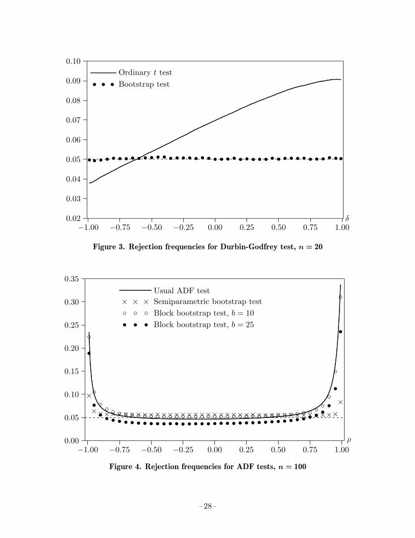
−1.00 −0.75 −0.50 −0.25 0.00 0.25 0.50 0.75 1.000.02

0.03

0.04

0.05

0.06

0.07

0.08

0.09

0.10

.......................................................

.......................................................

.........................................................

...........................................................

..........................................................

...........................................................

........................................................

.........................................................

............................................................

..........................................................

.............................................................

..............................................................

.................................................................

......................................................................

.............................................................................................

.........................................................................................................................

.......................................................................................... Ordinary t test

•• • • • • • • • • • • • • • • • • • • • • • • • • • • • • • • • • • • • • • ••

• • • Bootstrap test

δ

Figure 3. Rejection frequencies for Durbin-Godfrey test, n = 20

−1.00 −0.75 −0.50 −0.25 0.00 0.25 0.50 0.75 1.000.00

0.05

0.10

0.15

0.20

0.25

0.30

0.35

...........................................................................................................................................................................................................................................................................................................................................................................................................................................................................................................................................................................................................................................................................................................................................................................................................................................................................................................................................................................................................................................................................................................................

.............................................................

...................................................................................................................................................................................................................................................................................................................................................................................................................................................................

................................................................................................................ Usual ADF test

××××××××××××××××××××××××××××××××××××××××

×

× × × Semiparametric bootstrap test

•

•• • • • • • • • • • • • • • • • • • • • • • • • • • • • • • • • • •

• •••

•

• • • Block bootstrap test, b = 25 Block bootstrap test, b = 10

ρ

Figure 4. Rejection frequencies for ADF tests, n = 100

–28–

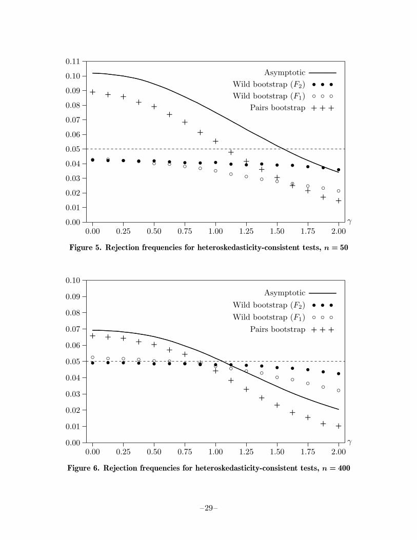
0.00 0.25 0.50 0.75 1.00 1.25 1.50 1.75 2.000.00

0.01

0.02

0.03

0.04

0.05

0.06

0.07

0.08

0.09

0.10

0.11..........................................................................................................................................................................................................................................................................................................................................................................................................................................................................................................................................................................................................................................................................................................................................................................................................................................................................................................................................................................................

...............................................................................................Asymptotic

• • • • • • • • • • • • • • • • •

• • •Wild bootstrap (F2)

Wild bootstrap (F1)+ + +

++

++

++

++

++

++

+ +

+ + +Pairs bootstrap

γ

Figure 5. Rejection frequencies for heteroskedasticity-consistent tests, n = 50

0.00 0.25 0.50 0.75 1.00 1.25 1.50 1.75 2.000.00

0.01

0.02

0.03

0.04

0.05

0.06

0.07

0.08

0.09

0.10

..................................................................................................................................................................................................................................................................................................................................................................................................................................................................................................................................................................................................................................................................................................................................................................................................................................................................................................................................................................

...............................................................................................Asymptotic

• • • • • • • • • • • • • • • • •

• • •Wild bootstrap (F2)

Wild bootstrap (F1)

+ + + + ++

++

++

++

++

++ +

+ + +Pairs bootstrap

γ

Figure 6. Rejection frequencies for heteroskedasticity-consistent tests, n = 400

–29–

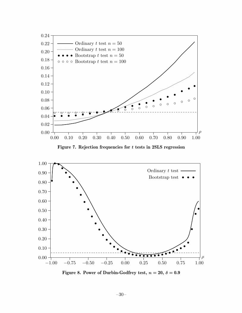
0.00 0.10 0.20 0.30 0.40 0.50 0.60 0.70 0.80 0.90 1.000.00

0.02

0.04

0.06

0.08

0.10

0.12

0.14

0.16

0.18

0.20

0.22

0.24

.......................................................................................................................................................................

...............................................................................

.................................................................

......................................................

..................................................

............................................

.........................................

.........................................

.........................................

..........................................

.......................................................................................................................................................................................................................................................................................................................................................................................................................................................................................................... Ordinary t test n = 50

.......................................

.................

..............

............

............

..........

..........

...........

..........

..........

.........

.....

................. Ordinary t test n = 100

• • • • • • • • • • • • • • • • • • • • •

• • • • Bootstrap t test n = 50

Bootstrap t test n = 100

ρ

Figure 7. Rejection frequencies for t tests in 2SLS regression

−1.00 −0.75 −0.50 −0.25 0.00 0.25 0.50 0.75 1.000.00

0.10

0.20

0.30

0.40

0.50

0.60

0.70

0.80

0.90

1.00

............

............

............

............

............

............

...........................................................................................................................................................................................................................................................................................................................................................................................................................................................................................................................................................................................................................................................................................................................................................................................................................................................................................................................................................................................................................................................

.....................................................................

........................................................

................................................

............................................................................................................................................................................................................................................................................

..........................................................................................Ordinary t test

•

• •••••••••••••• • • • • • • • • • • • • • • • • •

• • •• •

•

••

• • •Bootstrap test

ρ

Figure 8. Power of Durbin-Godfrey test, n = 20, δ = 0.9

–30–

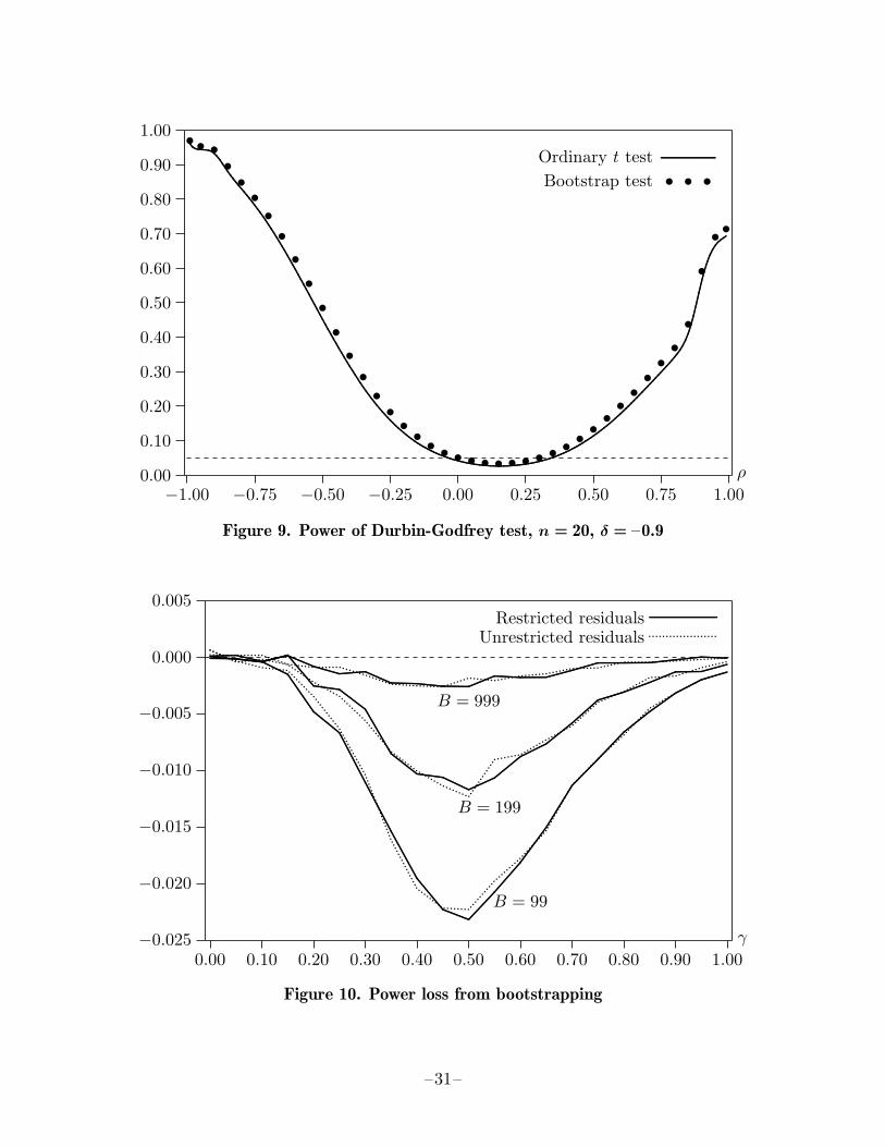
−1.00 −0.75 −0.50 −0.25 0.00 0.25 0.50 0.75 1.000.00

0.10

0.20

0.30

0.40

0.50

0.60

0.70

0.80

0.90

1.00..............................................................................................................................................................................................................................................................................................................................................................................................................................................................................................................................................................................................................................................................................................................................................................................................................................................................................................................................................................

..............................................................

................................................................................................................................................................................................................................................................................................................................................................................................................................................................................

..........................................................................................Ordinary t test•• •

••••••••••••• • • • • • • • • • • • •

• •• •

• •••••

•••

• • •Bootstrap test

ρ

Figure 9. Power of Durbin-Godfrey test, n = 20, δ = –0.9

0.00 0.10 0.20 0.30 0.40 0.50 0.60 0.70 0.80 0.90 1.00−0.025

−0.020

−0.015

−0.010

−0.005

0.000

0.005

....................................................................................................

................................................

....

....................Unrestricted residuals.........................................................................................................................................................................................................................................................................................................................................................................................................................................................................................

................................................................................................................................................................................

.......................................................................................................................................................................................................................................

...............................................................................................................Restricted residuals

..................................................................................................................................

.................................................................

.........

............

..............................................................................................................................................................................................................................................................................................................................................................................................................................................................................................................................................................................................................................................................................................

...............................................................................................................................................................................................................................................................................................................................................................................................................................................................................

...........................................

..........................................................

...........................

.............................................................................................................

..........

.........

..........

...........

..................

......................................................................................................................................................................................................................................................................................................................................................................................................................................................................................................................................................................................

....................................................................................

.................................................

..........................................................................................................................

.......................................................................

...............................................................................................................

.........................

B = 999

B = 199

B = 99

γ

Figure 10. Power loss from bootstrapping

–31–

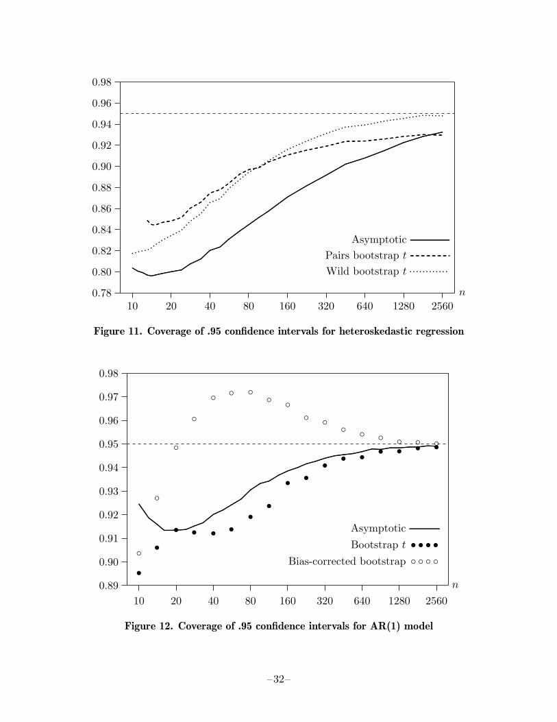
0.78

0.80

0.82

0.84

0.86

0.88

0.90

0.92

0.94

0.96

0.98

10 20 40 80 160 320 640 1280 2560

.........................................................................................................................................................

..................................................

........................................

..........................................................................................................

.........................................

...........................................

..............................................................

..............................................

.................................................

.................................................

...............................................................

...................................................................

...............................................................

..........................................................................................

............

......................................................................................................Asymptotic

..........................................................................

..........................

..................................................

..................................................

..................................................

...............................................

....................................................................

....................................................................................................................................

.............................................................................................

.........................................................................Pairs bootstrap t...........

.........

...........

...........

........

.........

............

......................

...............

............Wild bootstrap t

n

Figure 11. Coverage of .95 confidence intervals for heteroskedastic regression

0.89

0.90

0.91

0.92

0.93

0.94

0.95

0.96

0.97

0.98

10 20 40 80 160 320 640 1280 2560

...................................................................................................................................................................................................................

.........................................

.................................................

.............................................................................

.........................................................

...........................................................

.........................................................................

..........................................................................................................................

..............................................................................................................................................................................................

...............................................................................Asymptotic

•

•• • • •

••

• •• • • • • • •

• • • •Bootstrap t

Bias-corrected bootstrap

n

Figure 12. Coverage of .95 confidence intervals for AR(1) model

–32–