Boosting With the L2 Loss: Regression and...

This article was downloaded by: [Pennsylvania State University]On: 15 December 2014, At: 07:51Publisher: Taylor & FrancisInforma Ltd Registered in England and Wales Registered Number: 1072954 Registered office: MortimerHouse, 37-41 Mortimer Street, London W1T 3JH, UK

Journal of the American Statistical AssociationPublication details, including instructions for authors and subscription information:http://amstat.tandfonline.com/loi/uasa20

Boosting With the L2 LossPeter Bühlmanna & Bin Yua

a Peter Bühlmann is Associate Professor, Seminar für Statistik, ETH Zürich,CH-8032 Zürich, Switzerland . Bin Yu is Professor, Department of Statistics,University of California, Berkeley, CA 94720 . The authors thank Trevor Hastieand Leo Breiman for very helpful discussions and two referees for constructivecomments. Yu was partially supported by National Science Foundation grantsDMS-9803063 and FD01-12731 and Army Research Of. ce grants DAAG55-98-1-0341and DAAD19-01-1-0643.Published online: 31 Dec 2011.

To cite this article: Peter Bühlmann & Bin Yu (2003) Boosting With the L2 Loss, Journal of the American StatisticalAssociation, 98:462, 324-339, DOI: 10.1198/016214503000125

To link to this article: http://dx.doi.org/10.1198/016214503000125

PLEASE SCROLL DOWN FOR ARTICLE

Taylor & Francis makes every effort to ensure the accuracy of all the information (the “Content”)contained in the publications on our platform. However, Taylor & Francis, our agents, and our licensorsmake no representations or warranties whatsoever as to the accuracy, completeness, or suitabilityfor any purpose of the Content. Any opinions and views expressed in this publication are the opinionsand views of the authors, and are not the views of or endorsed by Taylor & Francis. The accuracy ofthe Content should not be relied upon and should be independently verified with primary sources ofinformation. Taylor and Francis shall not be liable for any losses, actions, claims, proceedings, demands,costs, expenses, damages, and other liabilities whatsoever or howsoever caused arising directly orindirectly in connection with, in relation to or arising out of the use of the Content.

This article may be used for research, teaching, and private study purposes. Any substantial orsystematic reproduction, redistribution, reselling, loan, sub-licensing, systematic supply, or distribution inany form to anyone is expressly forbidden. Terms & Conditions of access and use can be found at http://amstat.tandfonline.com/page/terms-and-conditions

http://amstat.tandfonline.com/loi/uasa20

http://amstat.tandfonline.com/action/showCitFormats?doi=10.1198/016214503000125

http://dx.doi.org/10.1198/016214503000125

http://amstat.tandfonline.com/page/terms-and-conditions

http://amstat.tandfonline.com/page/terms-and-conditions

Boosting With the L2 Loss:Regression and Classi� cation

Peter BÜHLMANN and Bin YU

This article investigates a computationally simple variant of boosting, L2Boost, which is constructed from a functional gradient descentalgorithm with the L2-loss function. Like other boosting algorithms, L2Boost uses many times in an iterative fashion a prechosen � ttingmethod, called the learner. Based on the explicit expression of re� tting of residuals of L2Boost, the case with (symmetric) linear learners isstudied in detail in both regression and classi� cation. In particular, with the boosting iteration m working as the smoothing or regularizationparameter, a new exponential bias–variance trade-off is found with the variance (complexity) term increasing very slowly as m tendsto in� nity. When the learner is a smoothing spline, an optimal rate of convergence result holds for both regression and classi� cationand the boosted smoothing spline even adapts to higher-order, unknown smoothness. Moreover, a simple expansion of a (smoothed) 0–1loss function is derived to reveal the importance of the decision boundary, bias reduction, and impossibility of an additive bias–variancedecomposition in classi� cation. Finally, simulation and real dataset results are obtained to demonstrate the attractiveness of L2Boost. Inparticular, we demonstrate that L2Boosting with a novel component-wise cubic smoothing spline is both practical and effective in thepresence of high-dimensional predictors.

KEY WORDS: Functional gradient descent; LogitBoost; Minimax error rate; Nonparametric classi� cation; Nonparametric regression;Smoothing spline.

1. INTRODUCTION

Boosting is one of the most successful and practical methodsthat has recently come from the machine learning community.Since its inception in 1990 (Schapire 1990; Freund 1995; Fre-und and Schapire 1996), it has been tried on an amazing array ofdatasets. The improved performance through boosting of a � t-ting method, called the learner, has been impressive and seemsto be associated with boosting’s resistance to over� tting. Theburning question is why this is so.

The rationale behind boosting diverges from that of the tra-ditional statistical procedures. It starts with a sensible estimatoror classi� er, the learner, and seeks its improvements iterativelybased on its performance on the training dataset. The possibil-ity of this boosting procedure comes with the availability oflarge datasets where one can easily set aside part of it as the testset (or use cross-validation based on random splits). It seem-ingly bypasses the need to get a model for the data and thepursuit of the optimal solution under this model as the com-mon practice in traditional statistics. For large dataset problemswith high-dimensional predictors, a good model for the prob-lem is hard to come by, but a sensible procedure is not. Thismay explain the empirical success of boosting on large, high-dimensional datasets. After much work on bounding the testset error (generalization error) of a boosted procedure via theVapnik– ÏCervonenkis (VC) dimensions and the distribution ofso-called margins (Schapire, Freund, Bartlett, and Lee 1998),some recent developments on boosting have been on the gra-dient descent view of boosting. These are the results of ef-forts of many researchers (e.g., Breiman 1999; Mason, Bax-ter, Bartlett, and Frean 2000; Friedman, Hastie, and Tibshirani2000; Collins, Schapire, and Singer 2000). This gradient de-scent view connects boosting to the more common optimiza-tion view of statistical inference; its most obvious consequence

Peter Bühlmann is Associate Professor, Seminar für Statistik, ETH Zürich,CH-8032 Zürich, Switzerland (E-mail: [email protected]). Bin Yuis Professor, Department of Statistics, University of California, Berkeley, CA94720 (E-mail: [email protected]). The authors thank Trevor Hastie andLeo Breiman for very helpful discussions and two referees for constructivecomments. Yu was partially supported by National Science Foundation grantsDMS-9803063 and FD01-12731 and Army Research Of� ce grants DAAG55-98-1-0341 and DAAD19-01-1-0643.

has been the emergence of many variants of the original Ada-Boost, under various loss or objective functions (Mason et al.2000; Friedman et al. 2000; Friedman 2001). Even though asatisfactory explanation of why boosting works does not fol-low directly from this gradient descent view, some of the newboosting variants are more easily accessible for analysis. In thisarticle we take advantage of this new analytic possibility on L2boosting procedures to build our case for understanding boost-ing in both regression and classi� cation. It is worth pointingoutthat L2Boost is studiedhere as a procedureyieldingcompetitivestatistical results in regression and classi� cation, in addition toits computational simplicity and analytical tractability.

After a brief overview of boosting from the gradient descentpoint of view in Section 2, the case of (symmetric) linear learn-ers in regression is covered in Section 3, building on the knownfact that L2Boost is a stagewise re� tting of the residuals (Fried-man 2001). We derive two main rigorous results:

1. With the boosting iteration m working as the smoothingor regularization parameter, a new exponential bias–var-iance trade-off is found. When the iteration m increasesby 1, one more term is added in the � tted procedure,but because of this new term’s dependence on the pre-vious terms, the “complexity” of the � tted procedure isincreased not by a constant amount as we became usedto in linear regression, but rather by an exponentially di-minishing amount as m gets large. At the iteration limit,the complexity or variance term is bounded by the noisevariance in the regression model.

2. When the learner is a smoothing spline, L2Boost achievesthe optimal rate of convergencefor one-dimensionalfunc-tion estimation. Moreover, this boosted smoothing splineadapts to higher-order, unknown smoothness.

Result 1 partially explains the “over� tting resistance” mysteryof boosting. This phenomenon is radically different from thewell-known algebraic bias–variance trade-off in nonparamet-ric regression. Result 2 gives an interesting result about boost-ing in adaptive estimation: Even when smoothness is unknown,L2Boost achieves the optimal (minimax) rate of convergence.

© 2003 American Statistical AssociationJournal of the American Statistical Association

June 2003, Vol. 98, No. 462, Theory and MethodsDOI 10.1198/016214503000125

324

Dow

nloa

ded

by [

Penn

sylv

ania

Sta

te U

nive

rsity

] at

07:

51 1

5 D

ecem

ber

2014

Bühlmann and Yu: Boosting With the L2 Loss 325

Section 4 proposes L2Boost with a novel componentwisesmoothing spline learner as a very effective procedure for car-rying out boosting for high-dimensional regression problemswith continuouspredictors. This proposed L2Boost is shown tooutperform L2Boost with stumps (i.e., a tree with two termi-nal nodes) and other more traditional competitors, particularlywhen the predictor space is very high dimensional.

Section 5 deals with classi� cation, � rst with the two-classproblem and then with the multiclass problem using the “oneagainst all” approach. The optimality in result 2 also holds forclassi� cation: L2Boost achieves the optimal (minimax) rate ofconvergence to the Bayes risk over an appropriate smoothnessfunction class, the risk of the best among all classi� cation pro-cedures. Section 6 also approximates the 0–1 loss function viaa smoothed version to show that the test set (generalization)er-ror of any procedure is approximately (in addition to the Bayesrisk) a sum of tapered moments. As a consequence of this ap-proximation,we gain more insight into why bias plays a biggerrole in 0–1 loss classi� cation than in L2 regression, why there iseven more “resistance against over� tting” in classi� cation thanin regression, and why previous attempts were not successfulat decomposing the test set (generalization) error into additivebias and variance terms (e.g., Geman, Bienenstock,and Doursat1992; Breiman 1998).

Section 7 provides support for the theory and explanationsfor classi� cation by simulated and real datasets that demon-strate the attractiveness of L2Boost. Finally, Section 8 containsa discussion on the role of the learner and a summary of thearticle.

2. BOOSTING: STAGEWISE FUNCTIONALGRADIENT DESCENT

The boosting algorithms can be seen as functional gradi-ent descent techniques. The task is to estimate the functionF : Rd ! R, minimizing an expected cost

E[C.Y;F .X//]; C.¢; ¢/ : R £ R ! RC (1)

based on data .Yi;Xi/ .i D 1; : : : ; n/. Here we consider caseswhere the univariate response Y is both continuous (regres-sion problem) and discrete (classi� cation problem), becauseboosting is potentially useful in both cases. Here X denotes ad-dimensional predictor variable. The cost function C.¢; ¢/ isassumed to be smooth and convex in the second argument, toensure that the gradient method works well. The most promi-nent examples are

C.y;f / D exp.yf / with y 2 f¡1; 1g: AdaBoost cost function;

C.y;f / D log2.1 C exp.¡2yf // with y 2 f¡1; 1g: LogitBoost

cost function; (2)

C.y;f / D .y ¡ f /2=2 with y 2 R or 2 f¡1;1g: L2Boost

cost function:

The population minimizers of (1) are then (Friedman et al.2000)

F.x/ D 1

2log

³P[Y D 1jX D x]

P[Y D ¡1jX D x]

´

for AdaBoost and LogitBoost cost; (3)

F .x/ D E[Y jX D x] for L2Boost cost:

Estimation of such an F .¢/ from data can be done via a con-strained minimization of the empirical risk,

n¡1nX

iD1

C.Yi ;F .Xi//; (4)

applying functional gradient descent. This gradient descentview has been recognized and re� ned by various authors, in-cluding Breiman (1999), Mason et al. (2000), Friedman et al.(2000), and Friedman (2001). In summary, the minimizer of (4)is imposed to satisfy a “smoothness” (or “regularization”) con-straint in terms of an additive expansion of (“simple”) learners(� tted functions),

h.x; Oµ/; x 2 Rd ;

where Oµ is an estimated � nite or in� nite-dimensionalparameter.For example, the learner h.¢; Oµ/ could be a decision tree whereOµ describes the axis to be split, the split points and the � ttedvalues for every terminal node (the constants in the piecewiseconstant � tted function). How to � t h.x; µ / from data is part ofthe learner and can be done according to a basis algorithm. Forexample, least squares � tting yields

OµU; X D argminµ

nX

iD1

.Ui ¡ h.XiI µ//2

for some data .U;X/ D f.Ui ;Xi/I i D 1; : : : ; ng. The generaldescription of functional gradient descent follows (see alsoFriedman 2001).

Generic functional gradient descent

Step 1 (initialization). Given data f.Yi ; Xi/I i D 1; : : : ; ng, � t areal-valued, (initial) learner,

bF0.x/ D h.xI OµY; X/:

When using least squares, OµY; X D argminµ

PniD1.Yi ¡

h.XiI µ//2 . Set m D 0.Step 2 (projection of gradient to learner). Compute the negativegradient vector,

Ui D ¡@C.Yi; F /

@F

F DbFm.Xi /

; i D 1; : : : ; n;

evaluated at the current bFm.¢/. Then � t the real-valued learnerto the gradient vector,

OfmC1.x/ D h.x; OµU; X/:

When using least squares, OµU; X D argminµ

PniD1.Ui ¡

h.XiI µ//2 .Step 3 (line search). Do one-dimensional numerical search forthe best step-size,

OwmC1 D argminw

nX

iD1

C.Yi ; bFm.Xi/ C wmC1 OfmC1.Xi//:

Update

bFmC1.¢/ D bFm.¢/ C OwmC1 OfmC1.¢/:

Step 4 (iteration). Increase m by 1, and repeat steps 2 and 3.The learner h.x; OµU; X/ in step 2 can often be viewed as an

estimate of E[Ui jX D x], and it takes values in R, even in case

Dow

nloa

ded

by [

Penn

sylv

ania

Sta

te U

nive

rsity

] at

07:

51 1

5 D

ecem

ber

2014

326 Journal of the American Statistical Association, June 2003

of a classi� cation problem with Yi in a � nite set. We call bFm.¢/the AdaBoost, LogitBoost, or L2Boost estimate, according tothe implementing cost function in (2).

L2Boost has a simple structure: The negative gradient inStep 2 is the classical residual vector, and the line search inStep 3 is trivial.

L2Boost algorithm

Step 1 (initialization). Follow step 1 of the generic functionalgradient descent, using a least squares � t (maybe includingsome regularization).Step 2. Compute residuals Ui D Yi ¡ bFm.Xi/ .i D 1; : : : ; n/ and� t the real-valued learner to the current residuals by (regular-ized) least squares as in step 2 of the generic functionalgradientdescent; the � t is denoted by OfmC1.¢/.Update

bFmC1.¢/ D bFm.¢/ C OfmC1.¢/:

Step 3 (iteration). Increase iteration index m by 1, and repeatstep 2.

L2 boosting is thus nothing else than repeated least squares� tting of residuals (Friedman 2001). With m D 1 (one boostingstep), it has already been proposed by Tukey (1977) under thename “twicing.”

For a continuousY 2 R, a regression estimate for E[Y jX D x]is directly given by the L2Boost estimate bFm.¢/. For a two-classproblem with Y 2 f¡1; 1g, a classi� er under equal misclassi� -cation costs is given by

sign.bFm.x//; (5)

because E[Y jX D x] D P[Y D 1jX D x] ¡ P[Y D ¡1jX D x].AdaBoost and LogitBoost estimates aim to estimate

F .x/ D 12

log

³P[Y D 1jX D x]

P[Y D ¡1jX D x]

´:

Hence an appropriate classi� er is again given by (5).Mason et al. (2000) and Collins et al. (2000) have described

when boosting-type algorithms (i.e., functional gradient de-scent) converge numerically. This tells us that under certainconditions, the test set (generalization)error for boosting even-tually stabilizes. But it does not imply that the eventually sta-ble solution is the best, or that over� tting could happen longbefore reaching convergence. Indeed, we show in Section 3that L2Boost with “contracting”linear learners convergesto thefully saturated model, that is, bF1.Xi/ D Yi for all i D 1; : : : ; n,� tting the data exactly.

Obviously, L2Boost and other functional gradient descentmethods depend on the choice of the learner. As the boostingiteration runs, the boosted procedure has more terms and hencebecomes more complex. It is intuitively clear that L2 boostingis not worthwhile if the learner is already complex (e.g., � ttingmany parameters), so that every boosting iteration contributesto additionalover� tting. We make this rigorous in Section 3 forlinear learners. Thus the learner in boosting should be “simple”;it typically involves only few parameters and has low variancerelative to bias. We say that such a learner is “weak,” an infor-mal terminology from machine learning. Weakness of a learnerdoes depend on the signal-to-noise ratio of the data; it is wellknown that if the noise level is low, a statistical method has

less a tendency to over� t. Of course, there are many possibili-ties for choosing a weak learner; examples include stumps thatare using trees with two terminal nodes only, using smoothingmethods with large amount of smoothing,or shrinking a learnerwith a small shrinkage factor. Illustrations of these are given inSections 3.2.2, 4.2, 7, and 8.

3. L2 BOOSTING WITH LINEAR LEARNERSIN REGRESSION

The nature of stagewise � tting is responsible to a large extentfor boosting’s resistance to over� tting. The same view has beenexpressed in Buja’s (2000) discussion of the article of Friedmanet al. (2000). He made amply clear there that this stagewise � t-ting had gotten a bad reputation among statisticians and wasnot getting the attention that it deserved. The success of boost-ing de� nitely serves as an eye-opener for us to take a fresh lookat stagewise � tting.

3.1 Theory

Consider the regression model

Yi D f .xi/ C "i ; i D 1; : : : ; n;

"1; : : : ; "n iid with E["i] D 0; var."i/ D ¾ 2; (6)

where f .¢/ is a real-valued, typically nonlinearfunction and thepredictors xi 2 Rd are deterministic (e.g., conditioning on thedesign).

We can represent a learner, evaluated at the predictorsx1; : : : ; xn as an operator S : Rn ! Rn , mapping the re-sponses Y1; : : : ; Yn to some � tted values in Rn . The predictorsx1; : : : ; xn are absorbed in the operator notationS . In the sequelwe often use the notation Y for the vector .Y1; : : : ; Yn/T and bFj

for the vector .bFj .x1/; : : : ; bFj .xn//T and analogously for Ofj ;it should always be clear from the context whether we mean asingle variable Y or function bFj .¢/, or the vectors as earlier.

Proposition 1. The L2Boost estimate in iteration m can berepresented as

bFm DmX

jD0

S.I ¡ S/j Y D .I ¡ .I ¡ S/mC1/Y:

A proof is given in the Appendix. We de� ne the boostingoperator Bm : Rn ! Rn as

Bm D I ¡ .I ¡ S/mC1

so that BmY D bFm.Proposition 1 describes an explicit relationship between the

boosting operator and the learner S . We exploit this in the se-quel.

We focus now on linear learners S . Examples include leastsquares � tting in linear models, more general projectors to agiven class of basis functions such as regression splines, andsmoothing operators such as kernel and smoothing spline esti-mators.

Proposition 2. Consider a linear learner S with eigen-values f¸kI k D 1; : : : ; ng, based on deterministic predictorsx1; : : : ; xn . Then the eigenvalues of the L2Boost operator Bm

are f.1 ¡ .1 ¡ ¸k/mC1I k D 1; : : : ; ng.

Dow

nloa

ded

by [

Penn

sylv

ania

Sta

te U

nive

rsity

] at

07:

51 1

5 D

ecem

ber

2014


Proof. This is a direct consequenceof Proposition 1.

Our analysis becomes even more transparent when special-ized to the case in which (the matrix) S D ST is symmetric.An important example is the smoothing spline operator (seeWahba 1990;Hastie and Tibshirani 1990),which is a more data-adaptive smoothing technique than, say, a kernel with a globalbandwidth. All eigenvalues of S are then real, and S as well asBm can be diagonalizedwith an orthonormal transform,

Bm D UDmUT ; Dm D diag.1 ¡ .1 ¡ ¸k/mC1/;

with the kth column vector of U being the ktheigenvector of S to the eigenvalue ¸k : (7)

The matrix U is orthonormal, satisfying UUT D UT U D I .We are now able to analyze a relevant generalizationmeasure

in this setting—the (averaged) mean squared error (MSE),

MSE D n¡1nX

iD1

E[.bFm.xi/ ¡ f .xi//2]; (8)

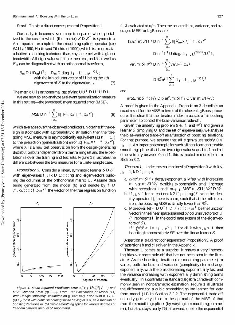
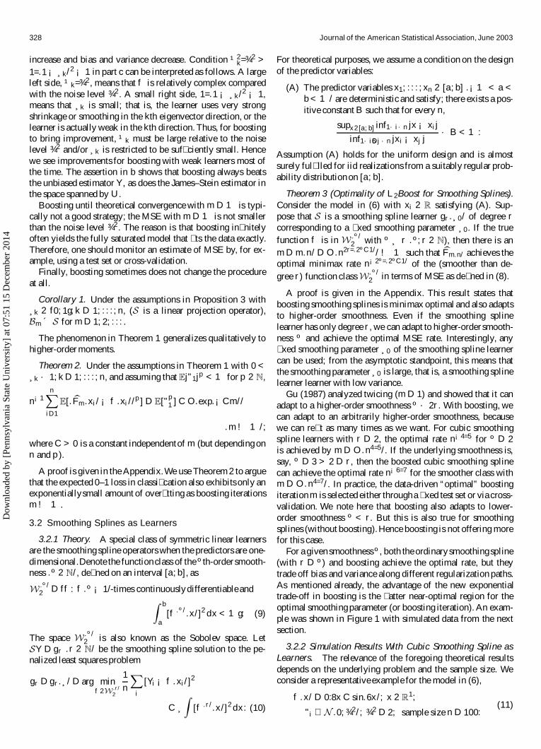
which averagesover the observed predictors.Note that if the de-sign is stochastic with a probability distribution, then the fore-going MSE measure is asymptotically equivalent (as n ! 1)to the prediction (generalization) error E[.bFm.X/ ¡ f .X//2],where X is a new test observation from the design-generatingdistributionbut independentfrom the training set and the expec-tation is over the training and test sets. Figure 1 illustrates thedifference between the two measures for a � nite-sample case.

Proposition 3. Consider a linear, symmetric learner S D ST

with eigenvalues f¸kIk D 1; : : : ; ng and eigenvectors build-ing the columns of the orthonormal matrix U . Assume databeing generated from the model (6) and denote by f D.f .x1/; : : : ; f .xn//T the vector of the true regression function

Figure 1. Mean Squared Prediction Error E[(Y ¡ Of (X))2 ] (—–) andMSE Criterion From (8) (.....). From 100 Simulations of Model (11)With Design Uniformly Distributed on [¡1=2;1=2], Each With n D 100.(a) L2Boost with cubic smoothing spline having df D 3, as a function ofboosting iterations m. (b) Cubic smoothing spline for various degrees offreedom (various amount of smoothing).

f .¢/ evaluated at xi’s. Then the squared bias, variance, and av-eraged MSE for L2Boost are

bias2.m; SI f / D n¡1nX

iD1

.E[bFm.xi/] ¡ f .xi//2

D n¡1f T U diag..1 ¡ ¸k/2mC2/UT f;

var.m; SI ¾ 2/ D n¡1nX

iD1

var.bFm.xi//

D ¾ 2n¡1nX

kD1

.1 ¡ .1 ¡ ¸k/mC1/2;

and

MSE.m;SI f; ¾ 2/ D bias2.m; SI f / C var.m;SI ¾ 2/:

A proof is given in the Appendix. Proposition 3 describes anexact result for the MSE in terms of the chosen L2Boost proce-dure. It is clear that the iteration index m acts as a “smoothingparameter” to control the bias–variance trade-off.

Given the underlying problem (i.e., f and ¾ 2) and given alearner S (implying U and the set of eigenvalues), we analyzethe bias–variance trade-off as a function of boosting iterations.For that purpose, we assume that all eigenvalues satisfy 0 <

¸k · 1. An importantexample for such a linear learner are cubicsmoothing splines that have two eigenvalues equal to 1 and allothers strictly between 0 and 1; this is treated in more detail inSection 3.2.

Theorem 1. Under the assumptions in Proposition3 with 0 <

¸k · 1; k D 1; : : : ; n,

a. bias2.mI SI f / decays exponentially fast with increasingm, var.m;SI ¾ 2/ exhibits exponentially small increasewith increasing m, and limm!1 MSE.m; SI f;¾ 2/ D ¾ 2.

b. If ¸k < 1 for at least one k 2 f1; : : : ; ng (S is not the iden-tity operator I ), there is an m, such that at the mth itera-tion, the boosting MSE is strictly lower than ¾ 2.

c. Moreover, let ¹ D UT f D .¹1; : : : ;¹n/T be the functionvector in the linear space spanned by column vectors of U

(¹ represents f in the coordinate system of the eigenvec-tors of S ).If ¹2

k=¾ 2 > 1=.1 ¡ ¸k /2 ¡ 1 for all k with ¸k < 1, thenboosting improves the MSE over the linear learner S .

Assertion a is a direct consequenceof Proposition 3. A proofof assertions b and c is given in the Appendix.

Theorem 1 comes as a surprise: it shows a very interest-ing bias–variance trade-off that has not been seen in the liter-ature. As the boosting iteration (or smoothing parameter) m

varies, both the bias and variance (complexity) term changeexponentially, with the bias decreasing exponentially fast andthe variance increasing with exponentially diminishing termseventually.This contrasts the standard algebraic trade-off com-monly seen in nonparametric estimation. Figure 1 illustratesthe difference for a cubic smoothing spline learner for datafrom model (11) in Section 3.2.2. The exponential trade-offnot only gets very close to the optimal of the MSE of thatfrom the smoothing splines (by varying the smoothing parame-ter), but also stays really � at afterward, due to the exponential

Dow

nloa

ded

by [

Penn

sylv

ania

Sta

te U

nive

rsity

] at

07:

51 1

5 D

ecem

ber

2014


increase and bias and variance decrease. Condition ¹2k=¾ 2 >

1=.1 ¡ ¸k/2 ¡ 1 in part c can be interpreted as follows. A largeleft side, ¹k=¾ 2 , means that f is relatively complex comparedwith the noise level ¾ 2 . A small right side, 1=.1 ¡ ¸k /2 ¡ 1,means that ¸k is small; that is, the learner uses very strongshrinkage or smoothing in the kth eigenvector direction, or thelearner is actually weak in the kth direction. Thus, for boostingto bring improvement, ¹k must be large relative to the noiselevel ¾ 2 and/or ¸k is restricted to be suf� ciently small. Hencewe see improvements for boosting with weak learners most ofthe time. The assertion in b shows that boosting always beatsthe unbiased estimator Y , as does the James–Stein estimator inthe space spanned by U .

Boosting until theoretical convergence with m D 1 is typi-cally not a good strategy; the MSE with m D 1 is not smallerthan the noise level ¾ 2 . The reason is that boosting in� nitelyoften yields the fully saturated model that � ts the data exactly.Therefore, one should monitor an estimate of MSE by, for ex-ample, using a test set or cross-validation.

Finally, boosting sometimes does not change the procedureat all.

Corollary 1. Under the assumptions in Proposition 3 with¸k 2 f0;1g; k D 1; : : : ; n, (S is a linear projection operator),Bm ´ S for m D 1; 2; : : : .

The phenomenon in Theorem 1 generalizes qualitatively tohigher-order moments.

Theorem 2. Under the assumptions in Theorem 1 with 0 <

¸k · 1; k D 1; : : : ; n, and assuming that Ej"1jp < 1 for p 2 N,

n¡1nX

iD1

E[.bFm.xi/ ¡ f .xi//p] D E["p

1 ] C O.exp.¡Cm//

.m ! 1/;

where C > 0 is a constant independentof m (but depending onn and p).

A proof is given in the Appendix.We use Theorem 2 to arguethat the expected 0–1 loss in classi� cation also exhibits only anexponentiallysmall amount of over� tting as boosting iterationsm ! 1.

3.2 Smoothing Splines as Learners

3.2.1 Theory. A special class of symmetric linear learnersare the smoothing spline operators when the predictors are one-dimensional.Denote the functionclass of the º th-order smooth-ness .º 2 N/, de� ned on an interval [a;b], as

W .º/2 D ff : f .º ¡ 1/-times continuouslydifferentiable and

Z b

a[f .º/.x/]2 dx < 1g: (9)

The space W .º/2 is also known as the Sobolev space. Let

SY D gr .r 2 N/ be the smoothing spline solution to the pe-nalized least squares problem

gr D gr .¸/ D arg minf 2W .r/

2

1n

X

i

[Yi ¡ f .xi/]2

C ¸

Z[f .r/.x/]2 dx: (10)

For theoretical purposes, we assume a condition on the designof the predictor variables:

(A) The predictor variables x1; : : : ; xn 2 [a;b] .¡1 < a <

b < 1/ are deterministic and satisfy; there exists a pos-itive constant B such that for every n,

supx2[a; b] inf1·i·n jx ¡ xijinf1·i 6Dj·n jxi ¡ xj j

· B < 1:

Assumption (A) holds for the uniform design and is almostsurely ful� lled for iid realizations from a suitably regular prob-ability distribution on [a; b].

Theorem 3 (Optimality of L2Boost for Smoothing Splines).Consider the model in (6) with xi 2 R satisfying (A). Sup-pose that S is a smoothing spline learner gr .¸0/ of degree r

corresponding to a � xed smoothing parameter ¸0 . If the truefunction f is in W .º/

2 with º ¸ r .º; r 2 N), then there is anm D m.n/ D O.n2r=.2ºC1// ! 1 such that bFm.n/ achieves theoptimal minimax rate n¡2º=.2ºC1/ of the (smoother than de-gree r) function class W .º/

2 in terms of MSE as de� ned in (8).

A proof is given in the Appendix. This result states thatboosting smoothing splines is minimax optimal and also adaptsto higher-order smoothness. Even if the smoothing splinelearner has only degree r , we can adapt to higher-order smooth-ness º and achieve the optimal MSE rate. Interestingly, any� xed smoothing parameter ¸0 of the smoothing spline learnercan be used; from the asymptotic standpoint, this means thatthe smoothing parameter ¸0 is large, that is, a smoothing splinelearner learner with low variance.

Gu (1987) analyzed twicing (m D 1) and showed that it canadapt to a higher-order smoothness º · 2r . With boosting, wecan adapt to an arbitrarily higher-order smoothness, becausewe can re� t as many times as we want. For cubic smoothingspline learners with r D 2, the optimal rate n¡4=5 for º D 2is achieved by m D O.n4=5/. If the underlying smoothness is,say, º D 3 > 2 D r , then the boosted cubic smoothing splinecan achieve the optimal rate n¡6=7 for the smoother class withm D O.n4=7/. In practice, the data-driven “optimal” boostingiteration m is selected either througha � xed test set or via cross-validation. We note here that boosting also adapts to lower-order smoothness º < r. But this is also true for smoothingsplines (without boosting). Hence boosting is not offering morefor this case.

For a given smoothnessº, both the ordinary smoothingspline(with r D º) and boosting achieve the optimal rate, but theytrade off bias and variance along different regularization paths.As mentioned already, the advantage of the new exponentialtrade-off in boosting is the � atter near-optimal region for theoptimal smoothing parameter (or boosting iteration). An exam-ple was shown in Figure 1 with simulated data from the nextsection.

3.2.2 Simulation Results With Cubic Smoothing Spline asLearners. The relevance of the foregoing theoretical resultsdepends on the underlying problem and the sample size. Weconsider a representative example for the model in (6),

f .x/ D 0:8x C sin.6x/; x 2 R1;

"i » N .0; ¾ 2/; ¾ 2 D 2; sample size n D 100:(11)

Dow

nloa

ded

by [

Penn

sylv

ania

Sta

te U

nive

rsity

] at

07:

51 1

5 D

ecem

ber

2014


The learner S is chosen as a cubic smoothing spline that satis-� es linearity, symmetry, and the eigenvalue conditions used inTheorems 1 and 2.

The complexity of S , or the strength of the learner, is chosenhere in terms of the so-called degrees of freedom (df), whichequals the trace of S (Hastie and Tibshirani 1990). To studythe interaction of the learner with the underlying problem, we� x the model as in (11) and a cubic smoothing spline learnerwith df D 20. To decrease the learner’s complexity (or increasethe learner’s weakness), we use shrinkage (Friedman 2001) toreplace S by

Sº D ºS; 0 < º · 1:

For S , a smoothingspline estimator, shrinkagewith º small cor-responds to a linear operator Sº whose eigenvalues fº¸kgk arecloser to 0 than f¸kgk for the original S . With small º, we thusget a weaker learner than the original S; here shrinkage actssimilarly as changing the degrees of freedom of the original Sto a lower value. We see its effect in more complex examplesin Sections 4.2 and 8. The boosting question becomes whethereven a very weak Sº , with º very small, can be boosted with m

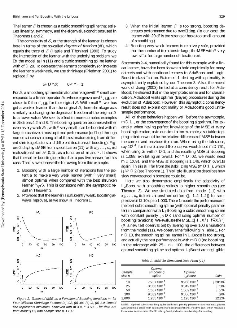
large to achieve almost-optimal performance (de� ned throughnumerical search among all of the estimators rising from differ-ent shrinkage factors and different iterations of boosting). Fig-ure 2 displays MSE from speci� cation (11) with x1; : : : ; xn iidrealizations from N .0; 1/, as a function of m and º. It showsthat the earlier boosting question has a positive answer for thiscase. That is, we observe the following from this example:

1. Boosting with a large number of iterations has the po-tential to make a very weak learner (with º very small)almost optimal when compared with the best shrunkenlearner ºoptS. This is consistent with the asymptotic re-sult in Theorem 3.

2. Provided that the learner is suf� ciently weak, boosting al-ways improves, as we show in Theorem 1.

Figure 2. Traces of MSE as a Function of Boosting Iterations m, forFour Different Shrinkage Factors: (a) .02, (b) .04, (c) .3, (d) 1.0. Dottedline represents minimum, achieved with m D 0, º D :76. The data arefrom model (11) with sample size n D 100.

3. When the initial learner S is too strong, boosting de-creases performance due to over� tting. (In our case, thelearner with 20 df is too strong or has a too small amountof smoothing.)

4. Boosting very weak learners is relatively safe, providedthat the number of iterations is large; the MSE with º verylow is � at for large number of iterations m.

Statements 2–4, numerically found for this example with a lin-ear learner, have also been shown to hold empirically for manydatasets and with nonlinear learners in AdaBoost and Logit-Boost in classi� cation. Statement 1, dealing with optimality, isasymptotically explained by our Theorem 3. Also, the recentwork of Jiang (2003) hinted at a consistency result for Ada-Boost; he showed that in the asymptotic sense and for classi� -cation, AdaBoost visits optimal (Bayes) procedures during theevolution of AdaBoost. However, this asymptotic consistencyresult does not explain optimality or AdaBoost’s good � nite-sample performance.

All of these behaviors happen well before the asymptopia,m D 1, or the convergence of the boosting algorithm. For ex-ample, when having perfect knowledge of the MSE at everyboosting iteration, as in our simulation example, a suitable stop-ping criterion would be the relative difference of MSE betweenthe current and previous iteration. When using the tolerance,say 10¡4, for this relative difference, we would need m D 761,when using Sº with º D 1, and the resulting MSE at stoppingis 1.088, exhibiting an over� t. For º D :02, we would needm D 1;691, and the MSE at stopping is 1.146, which over� tsagain.This is still far from the stabilizingMSE (m D 1), whichis ¾ 2 D 2 (see Theorem 1). This little illustration describes howslow convergence in boosting could be.

Here we also demonstrate empirically the adaptivity ofL2Boost with smoothing splines to higher smoothness (seeTheorem 3). We use simulated data from model (11) withx1; : : : ; xn iid realizations from uniform([¡1=2; 1=2]), for sam-ple sizes n D 10 up to 1,000.Table 1 reports the performance ofthe best cubic smoothing spline (with optimal penalty parame-ter) in comparison with L2Boosting a cubic smoothing splinewith constant penalty ¸0 D c (and using optimal number ofboosting iterations). We evaluate the MSE E[.f .X/ ¡ Of .X//2](X a new test observation) by averaging over 100 simulationsfrom the model (11). We observe the following in Table 1. Forn D 10, the smoothing spline learner in L2Boost is too strong,and actually the best performance is with m D 0 (no boosting).In the midrange with 25 · n · 100, the differences betweenoptimal smoothing spline and optimal L2Boost are negligible.

Table 1. MSE for Simulated Data From (11)

OptimalSample smoothing Optimalsize n spline L2 Boost Gain

10 7:787 ¢ 10¡1 9:968 ¢ 10¡1 ¡28:0%25 3:338 ¢ 10¡1 3:349 ¢ 10¡1 ¡:3%50 1:657 ¢ 10¡1 1:669 ¢ 10¡1 ¡:7%

100 9:332 ¢ 10¡2 9:050 ¢ 10¡2 :9%1;000 1:285 ¢ 10¡2 1:128 ¢ 10¡2 12:2%

NOTE: Optimal cubic smoothing spline (with best penalty parameter) and optimal L2Boostwith smoothing spline (with best number of boosting iterations). Positive gain, which measuresthe relative improvement of MSE with L2Boost, indicates an advantage for boosting.

Dow

nloa

ded

by [

Penn

sylv

ania

Sta

te U

nive

rsity

] at

07:

51 1

5 D

ecem

ber

2014


For the large sample size, n D 1;000, we see an advantage ofL2Boost that is consistent with the theory: The underlying re-gression function in (11) is in� nitely smooth, and L2Boost ex-hibits an adaptation to higher-order smoothness.

3.3 Estimating the Optimal Numberof Boosting Iterations

The number m of boosting iterations is a tuning parameterin L2 and other boosting methods. Theorem 1 and Figure 1 in-dicate a certain resistance against over� tting as m gets large,and thus the tuning of L2Boost should not be dif� cult. Never-theless, a method is needed to choose the value of m based ondata, or to estimate the optimal iteration number m.

A straightforward way that we found to work well isgiven by a � ve-fold cross-validation for estimating the MSEE[.Y ¡ bFm.X//2] in regression or the misclassi� cation errorP[sign.bFm.X// 6D Y ] in classi� cation. An estimate Om for thenumber of boosting iterations is then given as the minimizer ofsuch a cross-validated error.

4. L2 BOOSTING FOR REGRESSIONIN HIGH DIMENSIONS

When the dimension d of the predictor space is large, thelearner S is typically nonlinear. In very high dimensions, it be-comes almost a necessity to use a learner that is doing some sortof variable selection. One of the most prominent examples aretrees.

4.1 Componentwise Smoothing Splineas the Learner

As an alternative to tree learners with two terminal nodes(stumps), here we propose componentwise smoothing splines.A componentwise smoothing spline is de� ned as a smoothingspline with one selected explanatoryvariable xO¶ (O¶ 2 f1; : : : ; dg),where

O¶ D argmin¶

nX

iD1

.Yi ¡ Og¶.xi; ¶//2;

where Og¶ is the smoothing spline as de� ned in (10) using thepredictor x¶. Thus the componentwise smoothing spline learneris given by the function

OgO¶ : x 7! OgO¶.xO¶/; x 2 Rd :

Boosting stumps and componentwise smoothing splinesyields an additive model whose terms are � tted in a stagewisefashion. This is because an additive combination of a stumpor a componentwise smoothing spline bF0 C

PMmD1

Ofm , withOfm.x/ depending functionally only on xO¶m for some compo-

nent O¶m 2 f1; : : : ; dg, can be reexpressed as an additive function,PdjD1 Omj .xj /; x 2 Rd . The estimated functions Omj .¢/ when us-

ing boosting are � tted in stagewise fashion and different fromthe back� tting estimates in additive models (Hastie and Tib-shirani 1990). Boosting stumps or componentwise smoothingsplines is particularly attractive when aiming to � t an additivemodel in very high dimensions with d larger or of the orderof sample size n. Boosting has then much greater � exibilityto add complexity, in a stagewise fashion, to certain compo-nents j 2 f1; : : : ; dg and may even drop some of the variables

(components).We give examples in Section 4.2 illustrating thatwhen the dimension d is large, boosting outperforms the alter-native classical additivemodeling with variable selection,usingback� tting.

4.2 Numerical Results

We � rst consider the often-analyzeddataset of ozone concen-tration in the Los Angeles basin, which has been also consid-ered by Breiman (1998) in connection with boosting. The di-mension of the predictor space is d D 8, and the sample size isn D 330. Here we compare L2 boosting with classical additivemodels using back� tting and with multivariate adaptive regres-sion splines (MARS). L2Boost is used with stumps and withcomponentwise cubic smoothing splines with 5 df (Hastie andTibshirani 1990), and the number of iterations is estimated by� ve-fold cross-validation as described in Section 3.3. Additivemodel back� tting is used with the default smoothing splines inS-PLUS, and MARS is run by using the default parameters asimplemented in S-PLUS, library(mda), which is an additive � tusing a forward selection method (the default parameters do notallow for interactions). We estimate mean squared predictionerror, E[.Y ¡ bF .X//2] with bF .x/ D bE[Y jX D x], by randomlysplitting the data into 297 training observations and 33 test ob-servations and averaging 50 times over such random partitions;Table 2 displays the results. We conclude that L2Boost withcomponentwise splines is better than with trees and that it isamong the best, together with classical back� tting of additivemodels. Moreover, estimation of the number of boosting itera-tions works very satisfactorily, exhibiting a performance that isvery close to the optimum.

Next we show a simulated example in very high dimensionrelative to sample size, where L2Boost as a stagewise methodis better than back� tting for additive models with variable se-lection. The simulation model is

Y D100X

jD1

.1 C .¡1/j Aj Xj CBj sin.6Xj //

50X

jD1

.1 CXj =50/ C";

A1; : : : ;A100 iid unif.[0:6; 1]/;B1; : : : ;B100 iid unif.[0:8; 1:2]/; independent

from the Aj ’s; (12)

X » unif.[0; 1]100/ where all components areiid » unif.[0;1]/;

" » N .0;2/:

Samples of size n D 200 are generated from model (12);for each model realization (realized coef� cients A1; : : : ; A100;

Table 2. Cross-Validated Test Set MSEs for Ozone Data

Method MSE

L2Boost with componentwise spline 17:78L2Boost with stumps 21:33Additive model (back� tted) 17:41MARS 18:09

With optimal no. of iterations

L2Boost with componentwise spline 17:50 (5)L2Boost with stumps 20:96 (26)

NOTE: L2Boost with estimated and optimal (minimizing cross-validated test set error) numberof boosting iterations, given in parentheses. The componentwise spline is a cubic smoothingspline with df D 5.

Dow

nloa

ded

by [

Penn

sylv

ania

Sta

te U

nive

rsity

] at

07:

51 1

5 D

ecem

ber

2014


Table 3. MSEs for Simulated Data From (12) With n D 200

Method MSE

L2Boost with shrunken 11:87componentwise spline

L2Boost with shrunken stumps 12:76MARS 25:19Shrunken MARS 15:05

With optimal no. of iterations or variables

L2Boost with shrunken 10:69 (228)componentwise spline

L2Boost with shrunken stumps 12:54 (209)Additive model (back� tted and 16:61 (1)

forward selection)Shrunken additive model (back� tted and 14:44 (19)

forward selection)

NOTE: L2Boost with estimated and optimal (minimizing MSE) number of boosting iterations,given in parentheses; additive model with optimal number of selected variables, given in paren-theses. The componentwise spline is a cubic smoothing spline with df D 5; shrinkage factor isalways º D :5.

B1; : : : ; B50), we generate 200 iid pairs .Yi ;Xi/ .i D 1; : : : ;

n D 200/.We take the same approach as before, but using classical ad-

ditive modeling with a forward variable selection (inclusion)strategy because d D 100 is very large compared with n D 200;this should be similar to MARS which by default doesn’t allowfor interactions. We evaluate E[.bF .X/ ¡ E[Y jX]/2] (X a newtest observation) at the true conditional expectation, which canbe done in simulations. Already a stump appeared to be toostrong for L2Boost, and we thus used shrunken learners ºSwith º D :5 chosen ad hoc; we also allowed the nonboostingprocedures to be shrunken with º D :5. Table 3 shows the aver-age performance over 10 simulationsfrom model (12). L2Boostis the winner over additive models and MARS, and the compo-nentwise spline is a better learner than stumps. Note that onlythe methods in the upper part of Table 3 are fully data-driven(the additive model � ts use the number of variables minimiz-ing the true MSE). We believe that boosting has a clear ad-vantage over other � exible nonparametric methods mainly insuch high-dimensionalsituations, and not so much in exampleswhere the dimension d is “midrange” or even small relative tosample size.

For simulated data, assessing signi� cance for differencesin performance is easy. Because all of the different meth-ods are used on the same data realizations, pairwise com-parisons should be made. Table 4 displays the p values ofpaired Wilcoxon tests. We conclude that for this simulationmodel (12), L2Boost with componentwise smoothing spline is

Table 4. p Values From Paired Two-Sided Wilcoxon Tests forEqual MSEs

L2 Boost Shrunkenshrunken Shrunken additivestumps MARS model

L2Boost shrunken .193 .010 .004componentwise spline

L2Boost shrunken stumps .010 .014Shrunken MARS .695

NOTE: Simulated data from (12) with n D 200 and 10 independentmodel realizations. Low pvalues of two-sided tests are always in favor of the method in the row; that is, the sign of teststatistic always points toward favoring the method in the row. L2 Boost with the estimated numberof boosting iterations; speci� cation of the methods as in Table 3.

best and signi� cantly outperforms the more classical methods,such as MARS or additive models.

5. L2 BOOSTING FOR CLASSIFICATION

The L2Boost algorithm can also be used for classi� cation,and it enjoys a computational simplicity in comparison withAdaBoost and LogitBoost.

5.1 Two-Class Problem

Consider a training sample

.Y1;X1/; : : : ; .Yn;Xn/ iid; Yi 2 f¡1;1g; Xi 2 Rd :

(13)L2 boosting then yields an estimate bFm for the unknown func-tion E[Y jX D x] D 2p.x/ ¡ 1, where p.x/ D P[Y D 1jX D x];the classi� cation rule is given by (5). Note that also in two-classproblems, the generic functionalgradient descent repeatedly � tssome learner h.x; µ/ taking values in R.

In addition to the L2Boost algorithm, we propose a mod-i� cation called “L2Boost with constraints” (L2WCBoost). Itproceeds as L2Boost, except that bFm.x/ is constrained to bein [¡1; 1]: this is natural because the target F .x/ D E[Y jX Dx] 2 [¡1; 1] is also in this range.

L2WCBoost algorithm

Step 1. bF0.x/ D h.xI OµY; X/ by least squares � tting. Set m D 0.Step 2. Compute residuals Ui D Yi ¡ bFm.Xi/ .i D 1; : : : ; n/.Then � t .U1;X1/; : : : ; .Un; Xn/ by least squares,

OfmC1.x/ D h.x; OµU; X/:

Update

eFmC1.¢/ D bFm.¢/ C OfmC1.¢/

and

bFmC1.x/ D sign.eFmC1.x// min¡1; jeFmC1.x/j

¢:

Note that if jeFmC1.x/j · 1, the updating step is as in theL2Boost algorithm.Step 3. Increase m by 1 and go back to step 2.

5.1.1 Theory. For theoretical purposes, consider the modelin (13) but with � xed, real-valued predictors,

Yi 2 f¡1; 1g independent; P[Yi D 1jxi ] D p.xi/;

xi 2 R .i D 1; : : : ; n/: (14)

Estimating E[Y jxi] D 2p.xi/¡1 in classi� cation can be seen asestimating the regression function in a heteroscedastic model,

Yi D 2p.xi/ ¡ 1 C "i .i D 1; : : : ; n/;

where "i are independent mean 0 variables, but with variance4p.xi/.1 ¡ p.xi//. Because the variances are bounded by 1,the arguments in the regression case can be modi� ed to give theoptimal rates of convergence results for estimating p.

Theorem 4 (Optimality of L2Boost for Smoothing Splinesin Classi� cation). Consider the model in (14) with xi satisfy-ing (A); see Section 3.2.1. Suppose that p 2 W .º/

2 [see (9)] andthat S is a smoothing spline linear learner gr.¸0/ of degree r,corresponding to a � xed smoothing parameter ¸0 [see (10)]. If

Dow

nloa

ded

by [

Penn

sylv

ania

Sta

te U

nive

rsity

] at

07:

51 1

5 D

ecem

ber

2014


º ¸ r , then there is an m D m.n/ D O.n2r=.2ºC1// ! 1 suchthat bFm.n/ achieves the optimal minimax rate n¡2º=.2ºC1/ of the

smoother function class W .º/2 for estimating 2p.¢/ ¡ 1 in terms

of MSE as de� ned in (8).

It is well known that 2 times the L1 norm bounds from abovethe difference between the generalizationerror of a plug-in clas-si� er (expected0–1 loss error for classifying a new observation)and the Bayes risk (cf. theorem 2.3 of Devroye, Györ� , andLugosi 1996). Furthermore, the L1 norm is upper bounded bythe L2 norm. It follows from Theorem 4 that if the underlyingp belongs to one of the smooth function class W .º/

2 , then L2

boosting converges to the average Bayes risk (ABR),

ABR D n¡1nX

iD1

P[sign.2p.xi/ ¡ 1/ 6D Yi ]:

Moreover, the L2 bound implies the following.

Corollary 2. Under the assumptions and speci� cations inTheorem 4,

n¡1nX

iD1

P[sign.bFm.n/.xi// 6D Yi ] ¡ ABR D O.n¡º=.2ºC1//:

Because the functions in W .º/2 are bounded, using Hoeffd-

ing’s inequality we can show that for both terms in Corollary 2,replacing the average by an expectation with respect to a den-sity for x would cause an error of order o.n¡º=.2ºC1// becauseº=.2º C 1/ < 1=2. Hence the foregoing result also holds if wereplace the averaging by an expectation with respect to a ran-domly chosen x with a design density and replace the ABR bythe correspondingBayes risk.

For the generalizationerror with respect to a random x , Yang(1999) showed that the foregoing n¡º=.2ºC1/ rate is also mini-max optimal for classi� cation over the Lipschitz family L .º/

2 ,

L .º/2 D fp : kp.x C h/ ¡ p.x/k2 < Chº ; kpk2 < Cg; (15)

where kpk2 D .R

p2.x/ dx/1=2. Yang (1999) used a hypercube

subclass in L .º/2 to prove the lower bound rate n¡º=.2ºC1/. This

hypercube subclass also belongs to our W .º/2 . Hence the rate

n¡º=.2ºC1/ also serves as a lower bound for our W .º/2 . Thus we

have proved that the minimax optimal rate n¡º=.2ºC1/ of con-vergence for the classi� cation problem over the global smooth-ness class W .º/

2 .Marron (1983) gave a faster classi� cation minimax rate of

convergence n¡2º=.2ºC1/ for a more restrictive global smooth-ness class, and the same rate holds for us if we adopt that class.On the other hand, Mammen and Tsybakov (1999) considereddifferent function classes that are locally constrained near thedecision boundary and showed that a faster rate than the para-metric rate n¡1 can even be achieved. The local constrainedclasses are more natural in the classi� cation setting with the 0–1loss because, as seen from our smoothed 0–1 loss expansionin Section 6.1, the actions happen near the decision boundary.These new rates are achieved by avoiding the plug-in classi� -cation rules through estimating p. Instead, empirical minimiza-tion of the 0–1 loss functionover regularized classes of decision

regions is used. However, computationally such a minimiza-tion could be very dif� cult. It remains an open question asto whether boosting can achieve the new optimal convergencerates of Mammen and Tsybakov (1999).

5.2 Multiclass Problem

The multiclass problem has response variables Yi 2 f1;2;

: : : ; J g, taking values in a � nite set of labels. An estimated clas-si� er, under equal misclassi� cation costs, is then given by

bC .x/ D arg maxj 2f1;:::;J g

bP[Y D j jX D x]:

The conditionalprobability estimates Opj .x/ D bP[Y D j jX D x].j D 1; : : : ; J / can be constructed from J different two-classproblems, where each two-class problem encodes the eventsfY D jg and fY 6D j g, this is also known as the “one againstall” approach (Allwein, Schapire, and Singer 2001). Thus theL2Boost algorithm for multiclass problems works as follows:Step 1. Compute bF .j /

m .¢/ as an estimate of pj .¢/ with L2- orL2WCBoost (j D 1; : : : ; J ) on the basis of binary responsevariables

Y.j /i D

»1 if Yi D j

¡1 if Yi 6D j; i D 1; : : : ; n:

Step 2. Construct the classi� er as

bC m.x/ D arg maxj2f1;:::;J g

bF .j /m .x/:

The optimality results from Theorem 4 carry over to the mul-ticlass case. Of course, other codings of a multiclass probleminto multiple two-class problems can be done (see Allwein et al.2001). The “one against all” scheme did work well in the casesthat we were examining (see also Sec. 7.2).

6. UNDERSTANDING THE 0–1 LOSSIN TWO-CLASS PROBLEMS

6.1 Generalization Error via Tapered Momentsof the Margin

Here we consider again the two-class problem as in (13). Theperformance is often measured by the generalization error

P[sign.bFm.X// 6D Y ] D P[Y bFm.X/ < 0] D E[1[Y bFm.X/<0]];(16)

where P and E are over all of the random variables in the train-ing set (13) and the testing observation .Y;X/ 2 f¡1;1g £ Rd ,which is independent of the training set. Insights about the ex-pected 0–1 loss function in (16), the generalization error, canbe gained by approximating it, for theoretical purposes, with asmoothed version,

E[C° .Y bFm.X//];

C° .z/D³

1 ¡ exp.z=° /

2

´1[z<0] C exp.¡z=° /

21[z¸0]; ° > 0:

The parameter ° controls the quality of approximation.

Proposition 4. Assume that the distribution of Z D Y bFm.X/

has a density g.z/ that is bounded for z in a neighborhoodaround 0. Then

jP[Y bFm.X/ < 0] ¡ E[C° .Y bFm.X//]j

D O.° log.° ¡1// .° ! 0/:

Dow

nloa

ded

by [

Penn

sylv

ania

Sta

te U

nive

rsity

] at

07:

51 1

5 D

ecem

ber

2014


A proof is given in the Appendix. Proposition 4 shows thatthe generalization error can be approximated by an expectedcost function that is in� nitely often differentiable.

Proposition 4 motivates to study generalizationerror throughE[C° .Z/] with Z D Y bFm.X/. Applying a Taylor series expan-sion of C° .¢/ around Z¤ D Y F .X/, we obtain

E[C° .Z/] D E[C° .Z¤/] C1X

kD1

1k!

E£C.k/

° .Z¤/.Z ¡ Z¤/k¤:

(17)Thereby the variables Z and Z¤ denote the so-called estimatedand true margin; a positive margin denotes a correct classi� -cation (and vice versa), and the actual value of the margin de-scribes closeness to the classi� cation boundary fx : F .x/ D 0g.The derivatives of C° .¢/ are

C.k/° .z/ D 1

° kexp

³¡jzj

°

´.¡1[z<0] C .¡1/k1[z¸0]/: (18)

Using conditioning on the test observations .Y; X/, the mo-ments can be expressed as

E£C.k/

° .Z¤/.Z ¡ Z¤/k¤

DX

y2f¡1; 1g

ZC.k/

° .yF .x//ykbk .x/P[Y D yjX D x] dPX.x/;

bk.x/ D E[.bFm.x/ ¡ F .x//k]; where expectation

is over the training set in (13). (19)

Thereby PX.¢/ denotes the distribution of the predictors X.From (17) and (19), we see that the smooth approximation to

the generalizationerror of any procedure is essentially, in addi-tion to the approximate Bayes risk E[C° Z¤], the averaged (as

in (19)) sum of moments bk.x/, tapered by C.k/° .yF .x//=k!,

which decays very quickly as yF .x/ moves away from 0. Thisexploits from a different view, the known fact that only the be-havior of bk.x/ in the neighborhoodof the classi� cation bound-ary fxI F .x/ D 0g matters to the generalization error.

The � rst two terms in the approximation (17) are the taperedbias and the tapered L2 term; see (19) with k D 1 and 2. Thehigher-order terms can be expanded as terms of interactions be-tween the centered moments and the bias term (all tapered),

bk.x/ D E[.bFm.x/ ¡ F .x//k]

DkX

jD0

³k

j

´b1.x/j E[.bFm.x/ ¡ E[bFm.x/]/k¡j ]: (20)

This seemingly trivial approximation has three important con-sequences. The � rst consequence is that bias (after tapering) asthe � rst term in (17) and multiplicativeterms in highermoments[see (20)] plays a bigger role in (smoothed) 0–1 loss classi� ca-tion than in L2 regression. Second, in the case of boosting, be-cause all of the (tapered) centered moment terms bk.x/ in (19)are bounded by expressions with exponentiallydiminishing in-crements as boosting iterations m get large (see Sec. 3, particu-larly Theorem 2) we gain resistance against over� tting. In viewof the additional tapering, this resistance is even stronger than inregression (see the rejoinder of Friedman et al. 2000 for a rele-vant illustration). The third consequence of the approximations

in (17), (19), and (20) is to suggest why the previous attemptswere not successful at decomposing the 0–1 prediction (gener-alization) error into additive bias and variance terms (Gemanet al. 1992; Breiman 1998; references therein). This is because,except for the � rst two terms, all other important terms includethe bias term also in a multiplicative fashion [see (20)] for eachterm in the summation (17), instead of in a pure additive way.

We conclude heuristically that the exponentiallydiminishingincrease of centered moments as the number of boosting iter-ations grow (as stated in Theorem 2), together with the taper-ing in the smoothed 0–1 loss, yields the overall (often strong)over� tting-resistanceperformance of boosting in classi� cation.

6.2 Acceleration of F and Classi� cation Noise

As seen in Section 6.1, resistance against over� tting isclosely related to the behavior of F .¢/ at the classi� cationboundary. If the true F .¢/ moves away quickly from the clas-si� cation boundary fxI F .x/ D 0g, then the relevant taperingweights C

.k/° .yF .x// decay very fast. This can be measured

with grad.F .x//jxD0, the gradient of F at 0. F .¢/ is said tohave a large acceleration if its gradient is large (elementwise inabsolute values, or in Euclidean norm). Thus a large accelera-tion of F .¢/ should result in strong resistance against over� ttingin boosting.

Noise negatively affects the acceleration of F .¢/. Noise inmodel (13), often called “classi� cation noise,” can be thoughtofin a constructiveway. Consider a random variable W 2 f¡1; 1g,independent from .Y; X/ with P[W D ¡1] D ¼ , 0 · ¼ · 1=2.The noisy response variable is

eY D WY; (21)

changing the sign of Y with probability ¼ . Its conditionalprob-ability is easily seen to be

P[eY D 1jX D x] D P[Y D 1jX D x].1¡2¼/ C ¼;

0 · ¼ · 1=2: (22)

Denote by eF .¢/ the noisy version of F .¢/, with P[eY D 1jX D x]replacing P[Y D 1jX D x] for F .¢/ being either half of the log-odds ratio or the conditional expectation [see (3)]. A straight-forward calculation then shows

grad.eF .x//jxD0 & 0 as ¼ % 1=2: (23)

The noisier the problem, the smaller the acceleration of eF .¢/and thus the lower the resistance against over� tting, be-cause the tapering weights in (18) are becoming larger innoisy problems. This adds insights to the known empiri-cal fact that boosting does not work well in noisy prob-lems (see Dietterich 2000). Typically, over� tting then kicksin early, and many learners are too strong in noisy prob-lems. Using LogitBoost (Friedman et al. 2000), this effect isdemonstrated in Figure 3 for the breast cancer data availableat (http://www.ics.uci.edu/»mlearn/MLRepository), which hasbeen analyzed by many others. We see there that a stump al-ready becomes too strong for LogitBoost in the 25% or 40%noise-added breast cancer data.

Of course, adding noise makes the classi� cation problemharder. The optimal Bayes classi� er eC Bayes.¢/ in the noisy prob-

Dow

nloa

ded

by [

Penn

sylv

ania

Sta

te U

nive

rsity

] at

07:

51 1

5 D

ecem

ber

2014


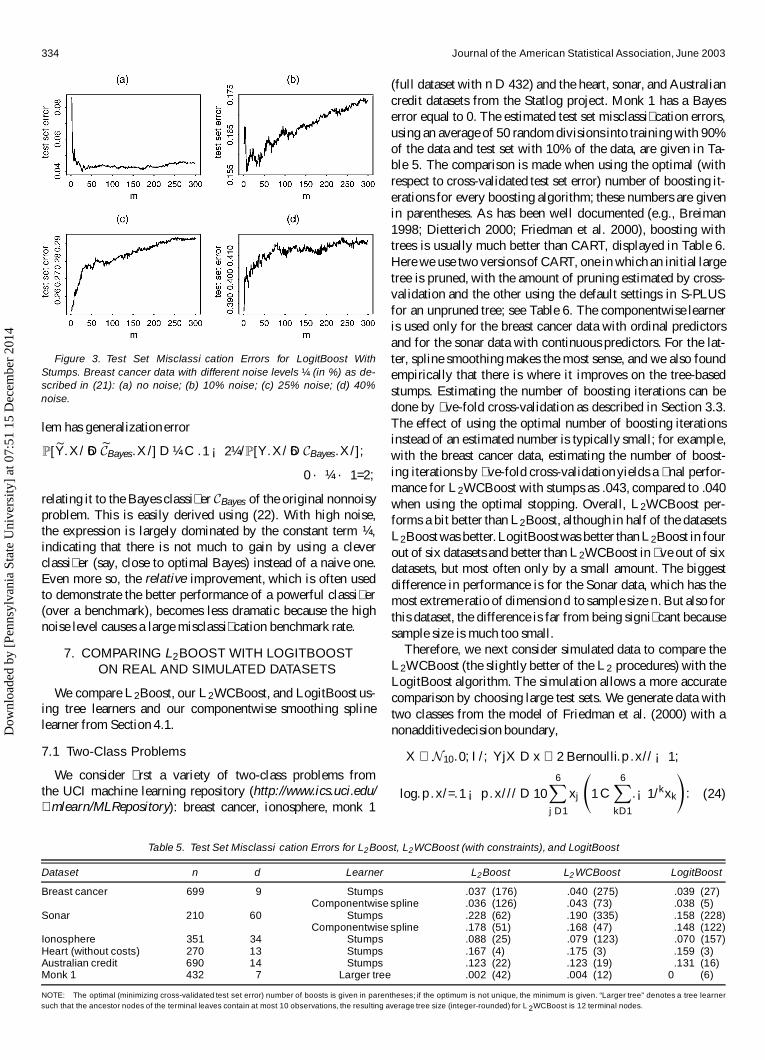
Figure 3. Test Set Misclassi�cation Errors for LogitBoost WithStumps. Breast cancer data with different noise levels ¼ (in %) as de-scribed in (21): (a) no noise; (b) 10% noise; (c) 25% noise; (d) 40%noise.

lem has generalization error

P[eY.X/ 6D eC Bayes.X/] D ¼ C .1 ¡ 2¼/P[Y .X/ 6D C Bayes.X/];

0 · ¼ · 1=2;

relating it to the Bayes classi� er C Bayes of the original nonnoisyproblem. This is easily derived using (22). With high noise,the expression is largely dominated by the constant term ¼ ,indicating that there is not much to gain by using a cleverclassi� er (say, close to optimal Bayes) instead of a naive one.Even more so, the relative improvement, which is often usedto demonstrate the better performance of a powerful classi� er(over a benchmark), becomes less dramatic because the highnoise level causes a large misclassi� cation benchmark rate.

7. COMPARING L2BOOST WITH LOGITBOOSTON REAL AND SIMULATED DATASETS

We compare L2Boost, our L2WCBoost, and LogitBoost us-ing tree learners and our componentwise smoothing splinelearner from Section 4.1.

7.1 Two-Class Problems

We consider � rst a variety of two-class problems fromthe UCI machine learning repository (http://www.ics.uci.edu/»mlearn/MLRepository): breast cancer, ionosphere, monk 1

(full dataset with n D 432) and the heart, sonar, and Australiancredit datasets from the Statlog project. Monk 1 has a Bayeserror equal to 0. The estimated test set misclassi� cation errors,using an average of 50 random divisions into training with 90%of the data and test set with 10% of the data, are given in Ta-ble 5. The comparison is made when using the optimal (withrespect to cross-validated test set error) number of boosting it-erations for every boosting algorithm; these numbers are givenin parentheses. As has been well documented (e.g., Breiman1998; Dietterich 2000; Friedman et al. 2000), boosting withtrees is usually much better than CART, displayed in Table 6.Here we use two versions of CART, one in which an initial largetree is pruned, with the amount of pruning estimated by cross-validation and the other using the default settings in S-PLUSfor an unpruned tree; see Table 6. The componentwise learneris used only for the breast cancer data with ordinal predictorsand for the sonar data with continuous predictors. For the lat-ter, spline smoothing makes the most sense, and we also foundempirically that there is where it improves on the tree-basedstumps. Estimating the number of boosting iterations can bedone by � ve-fold cross-validation as described in Section 3.3.The effect of using the optimal number of boosting iterationsinstead of an estimated number is typically small; for example,with the breast cancer data, estimating the number of boost-ing iterations by � ve-fold cross-validation yields a � nal perfor-mance for L2WCBoost with stumps as .043, compared to .040when using the optimal stopping. Overall, L2WCBoost per-forms a bit better than L2Boost, although in half of the datasetsL2Boost was better. LogitBoostwas better than L2Boost in fourout of six datasets and better than L2WCBoost in � ve out of sixdatasets, but most often only by a small amount. The biggestdifference in performance is for the Sonar data, which has themost extreme ratio of dimension d to sample size n. But also forthis dataset, the difference is far from being signi� cant becausesample size is much too small.

Therefore, we next consider simulated data to compare theL2WCBoost (the slightly better of the L2 procedures) with theLogitBoost algorithm. The simulation allows a more accuratecomparison by choosing large test sets. We generate data withtwo classes from the model of Friedman et al. (2000) with anonadditivedecision boundary,

X » N 10.0; I /; Y jX D x » 2 Bernoulli.p.x// ¡ 1;

log.p.x/=.1 ¡ p.x/// D 106X

jD1

xj

Á

1 C6X

kD1

.¡1/kxk

!

: (24)

Table 5. Test Set Misclassi�cation Errors for L2Boost, L2WCBoost (with constraints), and LogitBoost

Dataset n d Learner L2Boost L2 WCBoost LogitBoost

Breast cancer 699 9 Stumps .037 (176) .040 (275) .039 (27)Componentwise spline .036 (126) .043 (73) .038 (5)

Sonar 210 60 Stumps .228 (62) .190 (335) .158 (228)Componentwise spline .178 (51) .168 (47) .148 (122)

Ionosphere 351 34 Stumps .088 (25) .079 (123) .070 (157)Heart (without costs) 270 13 Stumps .167 (4) .175 (3) .159 (3)Australian credit 690 14 Stumps .123 (22) .123 (19) .131 (16)Monk 1 432 7 Larger tree .002 (42) .004 (12) 0 (6)

NOTE: The optimal (minimizing cross-validated test set error) number of boosts is given in parentheses; if the optimum is not unique, the minimum is given. “Larger tree” denotes a tree learnersuch that the ancestor nodes of the terminal leaves contain at most 10 observations, the resulting average tree size (integer-rounded) for L2WCBoost is 12 terminal nodes.

Dow

nloa

ded

by [

Penn

sylv

ania

Sta

te U

nive

rsity

] at

07:

51 1

5 D

ecem

ber

2014


Table 6. Test Set Misclassi�cation Errors for CART

Breast Australiancancer Sonar Ionosphere Heart credit Monk 1

Unpruned .060 .277 .136 .233 .151 .164CART

Pruned CART .067 .308 .104 .271 .146 .138

NOTE: Unpruned version with defaults from S-PLUS; pruning with cost-complexity parameter,estimated via minimal cross-validated deviance.

The (training) sample size is n D 2;000. It is interesting to con-sider the performance on a single set of training and test datathat resembles the situation in practice. Toward that end, wechoose a very large test set of size 100,000, so that variabilityof the test set error given the training data is very small. In addi-tion, we consider an average performance over 10 independentrealizations from the model; here we choose a test set size of10,000, which is still large compared with the training samplesize of n D 2;000. (The latter is the same setup as in Friedmanet al. 2000.)

Figure 4 displays the results on a single dataset. L2WCBoostand LogitBoost perform about equally well. L2WCBoost withthe larger regression tree learner having about nine terminalnodes has a slight advantage. Friedman et al. (2000) havepointed out that stumps are not good learners, because the truedecision boundary is nonadditive.With stumps as learners, theoptimally (minimizing test set error) stopped LogitBoost has atiny advantage over the optimally stopped L2WCBoost (betterby about .13 estimated standard errors for the test set error es-timate, given the training data). With larger trees, L2Boost hasa more substantial advantage over LogitBoost (better by about1.54 standard errors, given the data).

Figure 5 shows the averaged performance over 10 indepen-dent realizations with larger trees as learner; it indicates a moresubstantial advantage of L2WCBoost than on the single datarepresented by Figure 4. With 10 independent realizations, wetest whether one of the optimally (minimizing test set error)

Figure 4. Test Set Misclassi�cation Errors for a Single Realizationfrom Model (24). (a) Stumps as learner. (b) Larger tree as learner with atmost 175 observations per terminal node (the integer-rounded averagetree size for L2 WCBoost is 9 terminal nodes). (—— L2WCBoost; : : : : : : :

LogitBoost (in grey).)

Figure 5. Test Set Misclassi�cation Errors Averaged Over 10 Real-izations From Model (24). Larger tree as learner with at most 175 ob-servations per terminal node (the integer-rounded average tree size forL2 WCBoost is 9 terminal nodes). (—— L2 WCBoost; : : : : : : : LogitBoost(in grey).)

Table 7. Comparison of L2 WCBoost and LogitBoost: Two-SidedTesting for Equal Test Set Performance

t test Wilcoxon test Sign test

p value .0015 .0039 .0215

NOTE: Low p values are always in favor of L2WCBoost.

stopped Boosting algorithms yields a signi� cantly better testset misclassi� cation error. In 9 of the 10 simulations, optimallystopped L2WCBoost was better than LogitBoost. The p valuesfor testing the hypothesisof equal performance against the two-sided alternative are given in Table 7. Thus for the model (24)from Friedman et al. (2000), we � nd a signi� cant advantage ofL2WCBoost over LogitBoost.

It is not so surprising that L2WCBoost and LogitBoost per-form similarly. In nonparametric problems, loss functions areused locally in a neighborhood of a � tting point x 2 Rd ; anexample is the local likelihood framework (Loader 1999). Butlocally, the L2 and negative log-likelihood(with Bernoulli dis-tribution) losses have the same minimizers.

7.2 Multiclass Problems

We also ran the L2WCBoost algorithm using the “oneagainst all” approach described in Section 7.2 on two often-analyzed multiclass problems. The results are given in Table 8.The test set error curve remained essentially � at after the op-timal number of boosting iterations; for the Satimage data, therange of the test set error was [.096, .105] for iteration numbers148–800 (prespeci� ed maximum), whereas for the Letter data,the range was [.029, .031] for iteration numbers 460–1,000(prespeci� ed maximum). Therefore, a similar performance isexpected with estimated number of iterations.

In comparison to our results with L2WCBoost, Friedmanet al. (2000) obtained the following with their LogitBoost algo-rithm using the � xed number of 200 boosting iterations, .102with stumps and .088 with an 8-terminal node tree for the

Dow

nloa

ded

by [

Penn

sylv

ania

Sta

te U

nive

rsity

] at

07:

51 1

5 D

ecem

ber

2014


Table 8. Test Set Misclassi�cation Errors for L2WCBoost

No. ofDataset ntrain, ntest d classes Learner Error

Satimage 4,435, 2,000 36 6 stumps .110 (592)¼8 terminal .096 (148)

node treeLetter 16,000, 4,000 16 26 ¼30 terminal .029 (460)

node tree

NOTE: Optimal number of boosts (minimizing test set error) is given in parentheses; if theoptimum is not unique, the minimum is given. The approximate tree size is the integer-roundedaverage of tree sizes used during all 800 (Satimage) or 1,000 (Letter) boosting iterations.

Satimage data and .033 with an 8-terminal node tree for theLetter data. We have also tuned CART and obtained the follow-ing test set error rates: .146 for the Satimage and .133 for theLetter dataset.

Thus we � nd here a similar situation as for the two-classproblems. L2WCBoost is about as good as LogitBoost, andboth are better than CART (by a signi� cant amount for the letterdataset).

8. DISCUSSION AND CONCLUDING REMARKS

As seen in Section 3, the computationally simple L2 boost-ing is successful if the learner is suf� ciently weak (suf� cientlylow variance); see also Figure 2. If the learner is too strong (toocomplex), then even at the � rst boosting iteration, the MSE isnot improved over the original learner. Also in the classi� cationcase it is likely that the generalization error will then increasewith the number of boosting steps, stabilizing eventually dueto the numerical convergence of the boosting algorithm to thefully saturated model (at least for linear learners with eigen-values bounded away from 0). Of course, the weakness of alearner also dependson the underlyingsignal-to-noiseratio (seealso assertion c in Theorem 1). But the degree of weakness ofa learner can always be increased by an additional shrinkageusing Sº D ºS with shrinkage factor 0 < º < 1. For L2Boostwith one-dimensionalpredictors, we have presented asymptoticresults in Section 3.2 stating that boosting weak smoothingsplines is as good as or even better than using an optimal non-boosted smoothing spline, because boosting adapts to unknownsmoothness. In high dimensions, we see the most practical ad-vantages of boosting; we have exempli� ed this in Section 4.2.

The fact that the effectiveness of L2Boost depends on thestrength of the learner and the underlying problem is also (em-pirically) true for other variants of boosting. Figure 6 showssome results for LogitBoost with trees and with projection pur-suit learners having one ridge function (one term) for the breastcancer data. All tree learners are suf� ciently weak for the prob-lem, and the shrunken large tree seems best. Interestingly, theprojection pursuit learner is already strong, and boosting doesnot pay off. This matches the intuition that projection pursuitis very � exible, complex, and hence strong. Boosting projec-tion pursuit a second time (m D 2) reduces performance; thisestimate with m D 2 can then be improved by further boosting.Eventually the test set error curve exhibits over� tting and sta-bilizes at a relatively high value. We observed a similar patternwith projection pursuit learners in another simulated example.Such a multiminimum phenomenon is typically not found withtree learners, but it is not inconsistent with our theoretical argu-ments.

Figure 6. Test Set Misclassi�cation Errors of LogitBoost for BreastCancer Data. (a) Decision tree learners, namely stumps (—–), largeunpruned tree (¢ ¢ ¢ ¢) and shrunken large unpruned tree (- - - - -) withshrinkage factor º D :01. (b) Projection pursuit (PPR) learners, namelyone-term PPR (—–) and shrunken one-term PPR (¢ ¢ ¢ ¢) with shrinkagefactor º D :01.

Most empirical studies of boosting in the literature use a tree-structured learner. Their complexity is often low, because theyare themselves � tted by a stagewise selection of variables andsplit points, as in CART and other tree algorithms (whereasthe complexity would be much higher, or it would be a muchstronger learner, if the tree were � tted by a global search, whichis most often infeasible). When the predictor space is high di-mensional, the substantial amount of variable selection doneby a tree procedure is particularly helpful in leading to a low-complexity (or weak) learner. This feature may be very desir-able.

In this article, we mainly investigated the computationallysimple L2Boost by taking advantage of its analytical tractabil-ity, and we also demonstrated its practical effectiveness. Our� ndings can be summarized as follows:

1. L2Boost is appropriate for both regression and classi� ca-tion. It leads to competitive performance also in classi� -cation relative to LogitBoost.

2. L2Boost is a stagewise � tting procedure,with the iterationm acting as the smoothing or regularizationparameter (asis also true for other boosting algorithms). In the linearlearner case, m controls a new exponential bias–variancetrade-off.

3. L2Boost with smoothing splines results in optimal min-imax rates of convergence in both regression and clas-si� cation. Moreover, the algorithm adapts to unknownsmoothness.

4. Boosting learners that involve only one (selected) pre-dictor variable yields an additive model � t. We proposecomponentwise cubic smoothing splines of such type thatwe believe are often better learners than tree-structuredstumps, especially for continuouspredictors.

5. Weightingobservationsis not used for L2Boost; we doubtthat the success of general boosting algorithms is due to“giving large weights to heavily misclassi� ed instances”

Dow

nloa

ded

by [

Penn

sylv

ania

Sta

te U

nive

rsity

] at

07:

51 1

5 D

ecem

ber

2014


as Freund and Schapire (1996) conjectured for AdaBoost.Weighting in AdaBoost and LogitBoost comes as a con-sequence of the choice of the loss function and likely isnot the reason for their successes. It is interesting to notehere Breiman’s (2000) conjecture that even in the case ofAdaBoost, weighting is not the reason for success.

6. A simple expansion of the smoothed 0–1 loss reveals newinsights into the classi� cation problem, particularlyan ad-ditional resistance of boosting against over� tting.

APPENDIX: PROOFS

Proof of Proposition 1

For L2Boost with cost function C.y; u/ D .y ¡ u/2=2, the negativegradient in stage j is the classical residual vector uj D Y ¡ bFj¡1 andbFj D bFj¡1 C Ofj (there is no need for a line search) with Ofj D Suj .Thus

uj D Y ¡ bFj¡1 D uj¡1 ¡ Suj¡1 D .I ¡ S /uj¡1; j D 1;2; : : : ; m;

implying that uj D .I ¡ S/jY for j D 1;2; : : : ;m. Because bF0 D SY

we obtain bFm DPm

jD0 S .I ¡S /j Y . Using a telescope-sumargument,

this equals .I ¡ .I ¡ S/mC1/Y .


The bias term is

bias2.m;S If / D .E[BmY ] ¡ f /T .E[BmY ] ¡ f /

D ..Bm ¡ I /f /T ..Bm ¡ I /f /:

According to (7), using orthonormality of U ,

Bm ¡ I D U.Dm ¡ I /U T D U diag.¡.1 ¡ ¸k/mC1/U T :

Thus, again by orthonormality of U , the formula for the bias follows.For the variance, consider

cov.BmY / D Bm cov.Y /BTm D ¾ 2BmBT

m

D ¾ 2U diag..1 ¡ .1 ¡ ¸k/mC1/2/U T ;

using (7) and orthonormalityof U . Then

var.m;S I¾ 2/ D tr[cov.BmY /] D ¾ 2nX

kD1

.1 ¡ .1 ¡ ¸k/mC1/2;

again using orthonormalityof U .

Proof of Theorem 1

For assertion c, without loss of generality, assume that ¸k < 1 forall k. If not, then restrict the summation to those k’s that satisfy ¸k < 1.Denote ¹ D UT f 2 Rn . For x ¸ 0, let

g.x/ D n¡1nX

kD1

¹2k.1 ¡ ¸k/2xC2 C ¾ 2n¡1

nX

kD1

.1 ¡ .1 ¡ ¸k/xC1/2:

Then

g.m/ D MSE.m;S If;¾ 2/ D bias2.m;S If / C var.m;S I¾ 2/:

It is easy to derive

g0.x/ D 2n¡1nX

kD1

[.¹2k C ¾ 2/ .1 ¡ ¸k/xC1 ¡ ¾ 2]

£ .1 ¡ ¸k /xC1 log.1 ¡ ¸k/:

It follows that

g0.0/ D 2n¡1nX

kD1

[.¹2k C ¾ 2/.1 ¡ ¸k/ ¡ ¾ 2].1 ¡ ¸k/ log.1 ¡ ¸k /

and

g0.1/ D 2n¡1nX

kD1

[.¹2k C ¾ 2/.1 ¡ ¸k/2 ¡ ¾ 2].1 ¡ ¸k /2 log.1 ¡ ¸k/;

both of which are negative under the inequality condition ¹k=¾ 2 >

1=.1 ¡ ¸k /2 ¡ 1; also, g 0.x/ < 0 for x 2 .0;1/ under this condition.Hence g.1/ < g.0/, which means that boosting improves.

b. Rewrite

g.x/ D n¡1nX

kD1

[.¹2k C ¾ 2/.1 ¡ ¸k/xC1 ¡ 2¾ 2].1 ¡ ¸k/xC1 C ¾ 2:

Because for all k (with ¸k < 1), .¹2k C¾ 2/.1¡¸k /xC1 ¡2¾ 2 ! ¡2¾ 2

as x ! 1, there exists an m such that .¹2k C¾ 2/.1¡¸k/mC1 ¡2¾ 2 ·

¡¾ 2 for all k (with ¸k < 1). It follows that

g.m/ · ¡n¡1nX

kD1

.1 ¡ ¸k/mC1¾ 2 C ¾ 2 < ¾ 2:

It is obvious that g.m/ ! ¾ 2 as m ! 1.

Proof of Theorem 2

Write the summands with the higher-ordermoment as

E[.bFm.xi /¡f .xi//p ]

DpX

jD0

³p

j

´bm.xi /

j E[.bFm.xi / ¡ E[bFm.xi /]/p¡j ]; (A.1)

where bm.xi / D E[bFm.xi / ¡ f .xi /] is the bias term. Thus we havetransformed the higher-order moment as a sum of higher-order cen-tered moments with the bias as a multiplier that goes to 0 as m ! 1.The centered moments can be written as

.bFm.xi / ¡ E[bFm.xi/]/q D .BmY ¡ E[BmY ]/

qi

D .Bm"/qi

D ..I ¡ .I ¡ S /mC1/"/qi

D ." ¡ .I ¡ S/mC1"/qi ;

where we use Proposition 1. Because .I ¡ S /mC1 is a map (matrix)taking values exponentiallyclose to 0 as m ! 1, we obtain

E[.bFm.xi/ ¡ E[bFm.xi /]/q] D E["

qi ] C O.exp.¡Cqm// .m ! 1/

for some constant Cq > 0. From this last bound and using (A.1) to-gether with the fact that the bias bm.xi/ D O.exp.¡Cbm//.m ! 1/

for some constant Cb > 0 (see Theorem 1), we complete the proof.

Proof of Theorem 3

Let S be the smoothing spline operator corresponding to smooth-ness r and with smoothing parameter c D ¸0 (to avoid notational con-fusion with eigenvalues). It is well known (Utreras 1983; Wahba 1990,p. 61) that the eigenvalues of S take the form, in decreasing order,

¸1 D ¢ ¢ ¢ D ¸r D 1; ¸k Dnqk; n

n¸0 C nqk; nfor k D r C 1; : : : ; n:

Moreover, under assumption (A) and for n large, qk; n ¼ Ak¡2r :DAqk .0 < A < 1/ (Utreras 1988). For the true function f 2 W .º/

2 ,

1

n

nX

kDrC1

¹2kk2º · M < 1:

Dow

nloa

ded

by [

Penn

sylv

ania

Sta

te U

nive

rsity

] at

07:

51 1

5 D

ecem

ber

2014


Let c0 D c=A; then

¸k ¼ qk

c0 C qkfor k D r C 1; : : : ; n:

Then the bias term can be bounded as

bias2.m;S If / D 1

n

nX

kDrC1

.1 ¡ ¸k/2mC2¹2k

¼ 1

n

nX

kDrC1

.1 ¡ qk=.c0 C qk//2mC2k¡2º¹2kk2º

· maxkDrC1;:::;n

.1 ¡ qk=.c0 C qk//2mC2k¡2º

£1

n

nX

kDrC1

¹2kk2º

D maxkDrC1;:::;n

exp.h.k// £1

n

nX

kDrC1

¹2kk2º;

where

h.x/ D log[.1 ¡ x¡2r =.c0 C x¡2r//2mC2x¡2º ]

D .2m C 2/ log.1 ¡ 1=.c0x2r C 1// ¡ 2º log.x/:

Taking the derivative yields

h0.x/ D2r

x

1

c0x2r C 1

h.2m C 2/ ¡ º

r.c0x2r C 1/

i:

Hence for any given positive integer n1, if x · n1 and m ¸º2r .c0n2r

1 C 1/ ¡ 1, then h.x/ is increasing and so is exp.h.x//, and

exp.h.x// · exp.h.n1// D .1 ¡ 1=.c0n2r1 C 1//2mC2n¡2º

1 :

On [n1 C 1;n],

exp.h.x// · .1 ¡ 1=.c0n2r C 1//2mC2n¡2º1 :

Putting them together, we get, for any given n1 and m ¸º2r

.c0n2r1 C 1/ ¡ 1,

bias2.m; SI f / · Mn¡2º1 [2.1 ¡ 1=.c0n2r C 1//2mC2];

which is of the order O.n¡2º1 / for n1 ! 1 and n1 · n.

We now deal with the variance term. For any n1 > r ,

var.m;S I¾ 2/ D ¾ 2

n

nr C

nX

kDrC1

[1 ¡ .1 ¡ ¸k/mC1]2o

· ¾ 2n1

nC ¾ 2

n

nX

kDn1C1

[1 ¡ .1 ¡ ¸k/mC1]2 :D I1 C I2:

Because .1 ¡ x/a ¸ 1 ¡ ax for any x 2 [0; 1] and a ¸ 1,

1 ¡ .1 ¡ ¸k/mC1 · 1 ¡ [1 ¡ .m C 1/¸k] D .m C 1/¸k:

It follows that

I2 · ¾ 2

n

nX

kDn1C1

.m C 1/2¸2k ¼ ¾ 2.m C 1/2

n

nX

kDn1C1

1

.c0k2r C 2/2

· ¾ 2.m C 1/2

n

nX

kDn1C1

1

.c0k2r/2· ¾ 2.m C 1/2

n

Z 1

n1

1

.c0x2r /2 dx

D¾ 2.m C 1/2

c20.4r ¡ 1/n

n1=n4r1 · O.n1=n/

if we take m D m.n1/ D º2r .c0n2r

1 C 1/ ¡ 1 D O.n2r1 /. Hence, for this

choice of m.n1/,

var.m.n1/;S I¾ 2/ · O.n1=n/:

Together with the bound for the bias, we get

1

nMSE · O.n1=n/ C O.n

¡2º1 /;

which is minimized by taking n1 D O.n1=.2ºC1// and for m.n/ Dm.n1/ D O.n2r=.2ºC1//. The minimized MSE has the minimax op-

timal rate O.n¡2º=.2ºC1// of the smoother function class W .º/2 .


Denote C.z/ D 1[z<0]. We � rst show that

supjzj>° log.° ¡1/

jC.z/ ¡ C° .z/j D ° =2: (A.2)

By symmetry, it suf� ces to consider z > 0,

supz>° log.° ¡1/

jC.z/ ¡ C° .z/j D C° .° log.° ¡1//

D exp.¡ log.° ¡1//=2 D ° =2;

proving (A.2).On the other hand,

Z

jzj·° log.° ¡1/jC.z/ ¡ C° .z/jg.z/ dz

· supjzj·° log.° ¡1/

jg.z/j° log.° ¡1/ D O.° log.° ¡1//: (A.3)

Hence, by (A.2) and (A.3),

jE[C.Z/ ¡ C° .Z/]j

·³Z

jzj>° log.° ¡1/C

Z

jzj·° log.° ¡1/

´jC.z/ ¡ C° .z/jg.z/ dz

· ° =2 C O.° log.° ¡1//

D O.° log.° ¡1// .° ! 0/:

[Received August 2001. Revised June 2002.]

REFERENCES

Allwein, E., Schapire, R., and Singer, Y. (2001), “Reducing Multiclass to Bi-nary: A Unifying Approach for Margin Classi� ers,” Journal of MachineLearning Research, 1, 113–141.

Breiman, L. (1998), “Arcing Classi� ers,” The Annals of Statistics, 26, 801–824.(1999), “Prediction Games and Arcing Algorithms,” Neural Computa-

tion, 11, 1493–1517.(2000), “Some In� nity Theory for Predictor Ensembles,” Technical

Report 579, University of California, Berkeley, Dept. of Statistics.Buja, A. (2000), Comment on “Additive Logistic Regression: A Statistical View

of Boosting,” by J. H. Friedman, T. Hastie, and R. Tibshirani, The Annals ofStatistics, 28, 387–391.

Collins, M., Schapire, R. E., and Singer, Y. (2000), “Logistic Regression, Ada-Boost, and Bregman Distances,” in Proceedings of the Thirteenth AnnualConference on Computational Learning Theory.

Devroye, L., Györ� , L., and Lugosi, G. (1996), A Probabilistic Theory of Pat-tern Recognition, New York: Springer.

Dietterich, T. G. (2000), “An Experimental Comparison of Three Methods forConstructing Ensembles of Decision Trees: Bagging, Boosting, and Random-ization,” Machine Learning, 40, 139–157.

Freund, Y. (1995), “Boosting a Weak Learning Algorithm by Majority,” Infor-mation and Computation, 121, 256–285.

Freund, Y., and Schapire, R. E. (1996), “Experiments With a New Boosting Al-gorithm,” in Machine Learning: Proceedings of the Thirteenth InternationalConference, San Francisco: Morgan Kauffman, pp. 148–156.

Dow

nloa

ded

by [

Penn

sylv

ania

Sta

te U

nive

rsity

] at

07:

51 1

5 D

ecem

ber

2014


Friedman, J. H. (2001), “Greedy Function Approximation: A Gradient BoostingMachine,” The Annals of Statistics, 29, 1189–1232.

Friedman, J. H., Hastie, T., and Tibshirani, R. (2000), “Additive Logistic Re-gression: A Statistical View of Boosting” (with discussion), The Annals ofStatistics, 28, 337–407.

Geman, S., Bienenstock, E., and Doursat, R. (1992), “Neural Networks and theBias/Variance Dilemma,” Neural Computations, 4, 1–58.

Gu, C. (1987), “What Happens When Bootstrapping the Smoothing Spline?,”Communications in Statistics, Part A—Theory and Methods, 16, 3275–3284.

Hastie, T. J., and Tibshirani, R. J. (1990), Generalized Additive Models, Lon-don: Chapman and Hall.

Jiang, W. (2003), “Process Consistency for AdaBoost,” The Annals of Statistics,to appear.

Loader, C. (1999), Local Regression and Likelihood, New York: Springer.Mammen, E., and Tsybakov, A. B. (1999), “Smooth Discriminant Analysis,”

The Annals of Statistics, 27, 1808–1829.Marron, J. S. (1983), “Optimal Rates of Convergence to Bayes Risk in Non-

parametric Discrimination,” The Annals of Statistics, 11, 1142–1155.

Mason, L., Baxter, J., Bartlett, P., and Frean, M. (2000), “Functional GradientTechniques for Combining Hypotheses,” in Advances in Large Margin Clas-si� ers, eds. A. J. Smola, P. J. Bartlett, B. Schölkopf, and D. Schuurmans,Cambridge, MA: MIT Press.

Schapire, R. E. (1990), “The Strength of Weak Learnability,” Machine Learn-ing, 5, 197–227.

Schapire, R. E., Freund, Y., Bartlett, P., and Lee, W. S. (1998), “Boosting theMargin: A New Explanation for the Effectiveness of Voting Methods,” TheAnnals of Statistics, 26, 1651–1686.

Tukey, J. W. (1977), Exploratory Data Analysis, Reading, MA: Addison-Wesley.

Utreras, F. (1983), “Natural Spline Functions, Their Associated EigenvalueProblem,” Numer. Math., 42, 107–117.

(1988), “Convergence Rates for Multivariate Smoothing Spline Func-tions,” Journal of Approximation Theory, 52, 1–27.

Wahba, G. (1990), Spline Models for Observational Data, Philadelphia: Societyfor Industrial and Applied Mathematics.

Yang, Y. (1999), “Minimax Nonparametric Classi� cation—Part I: Rates ofConvergence,” IEEE Transactions on Information Theory, 45, 2271–2284.

Dow

nloa

ded

by [

Penn

sylv

ania

Sta

te U

nive

rsity

] at

07:

51 1

5 D

ecem

ber

2014

Boosting With the L2 Loss: Regression and...

Documents

Transcript of Boosting With the L2 Loss: Regression and...