Boosting the performance of computational fluid dynamics … · · 2017-01-18Paul R. Woodward, a*...

Available online at www.sciencedirect.com ProcediaComputerScienceProcedia Computer Science 00 (2009) 000–000

www.elsevier.com/locate/procedia

International Conference on Computational Science, ICCS 2010

Boosting the performance of computational fluid dynamics codes for interactive supercomputing

Paul R. Woodward,a* Jagan Jayaraja, Pei-Hung Lina, Pen-Chung Yewa, Michael Knoxa,Jim Greenskya,b, Anthony Nowatskia, and Karl Stoffelsa

aLaboratory for Computational Science & Engineering, University of Minnesota, 117 Pleasant St. S. E., Minneapolis, MN 55455, USAbIntel Corporation, Portland, Oregon, USA

Abstract

An extreme form of pipelining of the Piecewise-Parabolic Method (PPM) gas dynamics code has been used to dramatically increase its performance on the new generation of multicore CPUs. Exploiting this technique, together with a full integration ofthe several data post-processing and visualization utilities associated with this code has enabled numerical experiments in computational fluid dynamics to be performed interactively on a new, dedicated system in our lab, with immediate, user controlled visualization of the resulting flows on the PowerWall display. The code restructuring required to achieve the necessary CPU performance boost, as well as the parallel computing methods and systems used to enable interactive flow simulation are described. Requirements for these techniques to be applied to other codes are discussed, and our plans for toolsthat will assist programmers to exploit these techniques are briefly described. Examples showing the capability of the new system and software are given for applications in turbulence and stellar convection.

Keywords: computational fluid dynamics, programming for multicore processors, interactive simulation and visualization

1. Introduction

During the last three years, our team at the University of Minnesota’s Laboratory for Computational Science & Engineering (LCSE) has been redesigning our Piecewise-Parabolic Method (PPM) computational fluid dynamics codes (cf. [1] and references therein) in order to take advantage of multicore CPUs. This undertaking began in order to exploit the IBM Cell processor and, through collaborations with colleagues at the Los Alamos National Laboratory (LANL), to exploit the Roadrunner petascale computing system. Early experience with Cell showed us a means to achieve roughly a three-fold increase in our code’s performance on a single CPU core. The 8-core design of the Cell processor then meant that this performance boost was, in the fall of 2006, in excess of a factor of 20 over our code’s previous single-processor performance on computing platforms of that day, such as the Cray-XT3 or IBM BladeCenter that we were then using. In the intervening time, we have built in our lab a small

* Corresponding author. Tel.: 612-625-8049. E-mail address: [email protected].

c⃝ 2012 Published by Elsevier Ltd.

Procedia Computer Science 1 (2012) 2055–2064

www.elsevier.com/locate/procedia

1877-0509 c⃝ 2012 Published by Elsevier Ltd.doi:10.1016/j.procs.2010.04.230

Open access under CC BY-NC-ND license.

Open access under CC BY-NC-ND license.

http://www.elsevier.com/locate/procedia

http://dx.doi.org/10.1016/j.procs.2010.04.230

http://creativecommons.org/licenses/by-nc-nd/3.0/

http://creativecommons.org/licenses/by-nc-nd/3.0/

Author name / Procedia Computer Science 00 (2010) 000–000

computing system exploiting multicore processors from both IBM and Intel and used this performance boost to enable fully interactive numerical simulation of fluid flows with immediate flow visualization on our 15 Mpixel PowerWall display. Below, we describe the restructuring and program transformations that make our codes run well on multicore CPUs, the integration with the running code of what was formerly an entire sequence of utilities for post-processing the code output, and the new simulation and visualization control interface that enables all these elements to function under interactive user control. We believe that the principal enabling techniques of code transformation for high multicore performance and of integration of the numerical simulation and its visualization can be broadly applied. We are therefore undertaking the development of tools that will assist programmers to carry out the most tedious of these tasks. Although we came upon the code transformations that we use in the context of moving our codes to the IBM Cell processor, we have found that the benefits we see on this CPU are delivered by the same transformations on Intel multicore CPUs as well. Therefore we believe that if other codes adopt these same strategies, they should see a performance boost on most any multicore CPU. GPUs are a special case that we are now exploring, because of the very small on-chip data storage that they offer for each of their processor cores. It is not yet clear that our strategies can be successfully extended to these platforms, but as GPUs continue to evolve we expect such an extension to become much easier.

2. The Principal Barrier to Code Performance: Data Bandwidth

Our analysis of why our codes have for many years failed to live up to the promise of microprocessor perform-ance that is known to be achievable for the LinPack benchmark is not unusual. Much like the community at large, we attribute this failure to a paucity of memory bandwidth. However, in the case of our codes as formulated before 2006, the bandwidth deficiency responsible for the observed performance was not only between the processor and its main memory but also, we believe, between the processor’s L2 cache and the processor’s registers. Our codes, like many others in the computational fluid dynamics community, were expressed as a series of vectorizable loops. The vector lengths that we found to give the best performance were around 256 elements [2]. We expressed our entire hydrodynamics calculation for a single strip of grid cells as a long series of vector operations on operands the full length of the grid strip, which we kept, by means of a domain decomposition, at around 128 to 256 cells. The number of such operands involved, that is the active set of grid strip vectors that are held in the processor cache, totaled around 200 vectors. Using 32-bit arithmetic, which since about 1992 we have used whenever possible, this active working data context for the hydrodynamics calculation amounts to about 200 KB. This data context fits into a standard L2 cache, but not into the L1 cache. In order to construct these long vectors, we also needed to transpose the fundamental data used by the calculation repeatedly, sweeping through the data stored at a given network node in a series of 1-D passes in the 3 grid directions. By 2006, this data transposition requirement of our approach was costing us up to about 40% of the running time. This meant that during nearly half of the time we rearranged the data in memory but performed no floating point arithmetic at all.

In our code’s present implementation, we have attacked both of the memory bandwidth problems identified above. First, we almost completely eliminate the cost of data transpositions by restructuring our data representing the fluid state in main memory so that it consists of a regular 3-D Fortran array of grid briquette records, with each record containing the entire fluid state data for a briquette of 23 grid cells. For our present two-fluid PPM code, we store 15 fluid state variables for each grid cell, so that this briquette record consists of 480 bytes, or just under 4 cache lines (for our single-fluid code, we use briquettes of 43 cells to achieve a similar data record size). These data records can be read, if they are read all at once, very efficiently from anywhere in the main memory. We find that transposing the contents of such data briquettes once they are in the cache is not a significant performance hit. Using this data structure therefore accelerates our code’s performance directly by almost a factor of 2. We obtain a comparable performance boost by restructuring the computation that takes place on the cached data, so that essentially the entire computation takes place in the L1 cache. This, we believe, is best done by reducing the vector length from 256 to 16. We do not do this by strip mining our vector loops. Instead, we effectively interchange the order of loop indices so that we vectorize in the transverse dimensions to the grid strip.

Our PPM codes have operated upon bundles of grid strips, which we call grid pencils, for decades. On microprocessors of the 1990s, we found that grid pencils 8 cells wide in each of the two grid dimensions transverse

2056 P.R. Woodward et al. / Procedia Computer Science 1 (2012) 2055–2064


to the direction of the 1-D pass were optimal, although we often used grid pencils 4 cells wide in order to expose more parallelism on multiprocessor systems. We described this mode of parallel code implementation and the several reasons that motivate it in 1998 in [3]. In working with the Cell processor using its library of vector intrinsics, we came to realize that the formulation of our algorithms in terms of long vectors in the direction of the 1-D pass forces the processor to constantly realign vector operands so that its 4-way SIMD floating point engine can process them in parallel. We then realized that all this realignment work can be eliminated by vectorizing over the 16 cells in each transverse grid plane of a long grid pencil 4 cells across in each transverse dimension. We found it quite surprising but nevertheless true that use of these tiny 16-element-long vectors proved extremely efficient. A benefit of this approach was that our entire working data context of about 200 vectors therefore shrank from 200 KB to under 13 KB, bringing the entire computation into the L1 cache. Once we achieved this benefit, we found that processor performance began once again to resemble our experience from the end of the vector computing era, circa 1990. We did not achieve the 50% of peak performance common in those days for our codes, but we found that 25 to 30% was possible, when averaged over our entire code including all costs of the computation (that is, including all network messaging and data I/O). For our codes, this represented a performance boost on a per-core basis of roughly a factor of 3. The extreme form of computation pipelining that we use brings the entire 1-D pass update of our algorithm, involving about 1400 vector floating point operations per grid cell into the L1 cache. To feed this computation, we need only bring in from main memory 15 words and write out 15 words per grid cell, so that running at 6 Gflop/s a single CPU core requires delivery of only about 245 MB/sec both to and from main memory simultaneously. This data streaming rate is not the performance limiting feature of our algorithms, even on CPUs containing as many as 8 cores. The specific means by which we achieve these significant benefits for our codes are outlined in the next section.

3. The Solution: Extreme Pipelining of the Computation

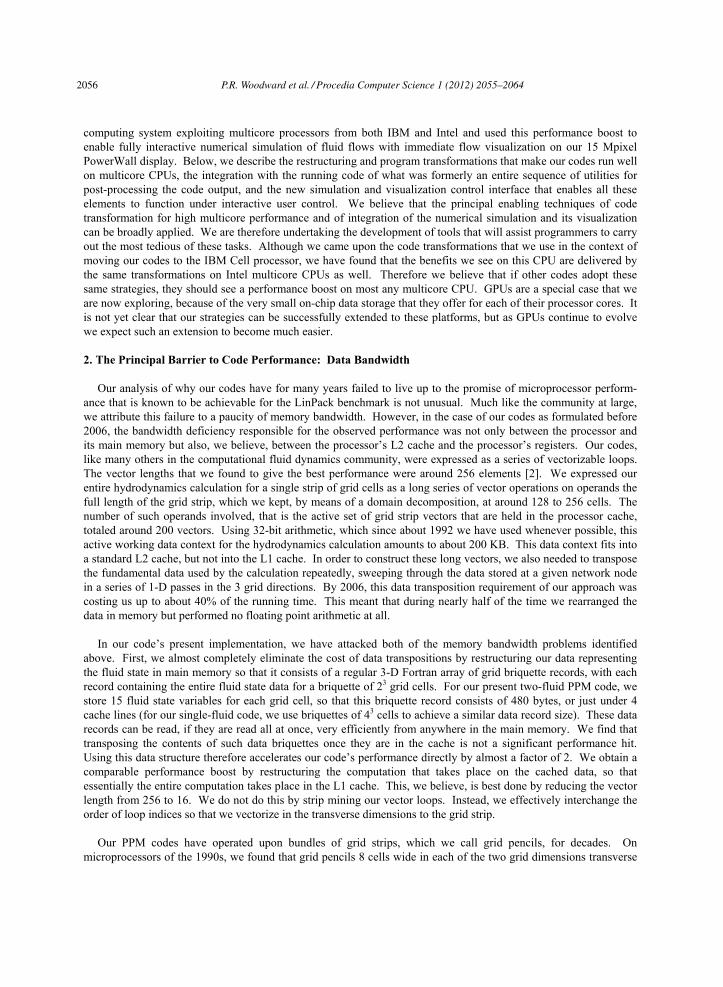
We have explained above that we decompose our fluid state data in main memory into an array of grid briquette data records. Using briquettes of 23 cells each, we read and write these in groups of 4 in order to process grid pencils that are, for example, 42×32 cells (see Figure 1). A single processor core that is working its way down the length of such a grid pencil can be prefetching from main memory the next group of 4 briquette records while it is updating the previous group and while it is writing back to main memory the updated records from a still earlier group. This process is illustrated in Figure 1. Here we take the trouble to explicitly overlap our data transfers from and to main memory with computation, which is a technique familiar from asynchronous message passing on a network or from asynchronous I/O to disk. The point is that the main memory in a modern multicore computer is best treated in this way, because it is very slow in comparison to the rate at which the CPU can process data. On the Cell processor, we are able to explicitly express this prefetching and asynchronous writing back of data to memory, while on Intel CPUs we simply express the data transfers in loops that copy data from/to memory to/from tiny arrays on the subroutine stack, which we can expect to be cache resident. The briquette records in main memory are copied into briquette records in cache (the subroutine stack), and then these are unpacked to form arrays (vectors) of 16 elements representing single planes of grid cells oriented transverse to the direction of the 1-D pass. We exploit the fact that our 1-D passes involve almost exclusively derivatives in the direction along the grid pencil. The corresponding data differences can then be computed from 16-long aligned vectors in the cache. No rearrangement of the native quadword data structures of the CPU core need to be performed. Thus this computation is exception-ally efficient. To handle aspects of the algorithm such as Navier-Stokes viscosity or subgrid-scale turbulence models, a few transverse derivatives must be taken. These are handled by constructing, using the transverse “ghost briquettes” shown in blue in Figure 1, aligned 16-word vectors representing quantities that are offset by one or by two cells in a transverse direction. Construction of the vectors representing 2-cell offsets, which are needed for our algorithm’s strong shock detection mechanism, is extremely fast, because no rearrangement of data inside individual quadwords is required.

To make the update of the grid pencil fully efficient, we need to make sure that we read each briquette record only once in a single 1-D pass. Since the algorithm requires transverse ghost briquettes, this is unlikely to be possible. However, if 8 cores on a single CPU chip sharing a common L2 or L3 cache update grid pencils together, then one core’s ghost briquette can serve as another’s core briquette, so that it need not be read in quite so many

P.R. Woodward et al. / Procedia Computer Science 1 (2012) 2055–2064 2057


times. We can therefore coordinate the updating of grid pencils on multicore CPUs to obtain this benefit, as indicated at the upper right in Figure 1. This coordination is easily accomplished; it is the pipelining of the entire grid cell update process that allows each core to read a briquette only once per 1-D pass that is difficult. In our PPM gas dynamics codes, we have performed this pipelining process manually so far. It results in a code in which the entire grid plane update is expressed in a single subroutine of thousands of lines of Fortran. Keeping the working data context small, so that the computation fits into the L1 cache, requires explicit reuse of multi-plane temporary vectors. The indexing of these vector temporaries is baroque (cf. [4-6]). The programming effort required to produce such a code, modify it, debug it, and maintain it is excessive. We regard our manually generated codes of this type as demonstration prototypes. They run on standard clusters of multicore CPU nodes, and they also run on the Los Alamos Roadrunner system, in which Cell processors are the principal computational engines. The performance of these codes is so greatly enhanced over our earlier experience that we do not want to give them up, but continuing to extend and maintain them is a burden. We are therefore building code translation tools to automate the transformations that take Fortran code written in a clear and simple fashion into these “compiled Fortran” expressions that boost its performance by factors of 3 or more.

4. Reducing the Programming Burden

We have begun the process of building code translation tools to automate the very labor intensive and error prone

Figure 1. At the left, a grid pencil is indicated within its larger grid brick data structure. It consists of a core of 22×16 grid briquettes, shown in red, surrounded by transverse “ghost briquettes” shown in blue and with longitudinal ghost briquettes shown in yellow. A CPU core works its way down this grid pencil (from left to right in the figure) pulling into its cache memory groups of 4 core and 8 transverse ghost briquettes as shown. These are unpacked to produce vectors representing the 16 cells of single transverse core grid planes as indicated at the bottom right. These form the working data in the L1 cache for 16-long, aligned vector operations. Differences to obtain derivatives in this 1-D pass are formed by subtracting neighboring grid plane vectors along the longitudinal direction of the pass. The transverse ghost briquettes are used to construct, in the cache, 16-long vectors representing grid planes offset by one or two cells in a transverse direction. At the top right in the Figure, we illustrate how 8 processor cores may simultaneously update neighboring grid pencils. The ghost briquettes of one such grid pencil may be core briquettes of a neighboring one, so that they need be fetched from main memory only once into a shared on-chip data cache. This is a streaming paradigm of vector computation that works exceptionally well on modern multicore CPUs.



transformations that we have been doing manually over the last 3 years. We are basing these tools on ANTLR, the source-to-source translating framework built by Terence Parr [7]. Parr used this framework in the early 1990s to automate translation of our PPM codes from standard Fortran into a very peculiar CM-Fortran expression that ran exceptionally well on the University of Minnesota’s Connection Machine CM5 at the time. ANTLR is appropriate to our present task, because we do not need to write a compiler, but only re-express the high-level Fortran code in a way that existing compilers can turn into high performance code for multiple target machines. Jayaraj and Lin are building our tools, and they have begun by using ANTLR to construct a translator that produces Cell-specific C with vector intrinsics from our “compiled Fortran” in order to run on the Roadrunner system and on a set of 6 Roadrunner-type nodes that we have in our lab. The code expression type that we are planning to support as input to our translator is not any form that we have used in any of our earlier codes. Instead, it is a format that we have seen in meteorological codes as well as in magnetohydrodynamic (MHD) simulation codes. Our idea is that the programmer can express the algorithm for updating a single grid brick with a uniform 3-D Cartesian mesh as a series of 3-D loop nests that go over this grid brick plus ghost cells augmenting it. This expression can involve multiple subroutines, of course. Our translation tool will pipeline this entire computation, responding to programmer directives, as a single outer loop in a single subroutine. The body of this outer loop will consist of a series of vector loops with tests and jumps to the end of the outer loop in between some of these inner loops (cf. [5,6]). This is basically the same program transformation that we described in [3] at a lower level of dimensionality and that, with that lower dimensionality, we used in alternative expressions of our sPPM benchmark code in the late 1990s. The higher dimensionality of this code transformation that we use today permits vector computation throughout, which is preferred by today’s microprocessors.

It should be clear from this brief discussion that a uniform Cartesian grid is a requirement for this high-level code transformation, at least at present. This uniformity of the grid need not, however, be global. We believe that in addition to the computational astrophysics domain, meteorology and climate simulation are domains that should be able to benefit relatively easily from the tools we are building. Adaptive mesh refinement (AMR) grids present some difficulties, but block-based AMR should be able to benefit without much modification to the input code expression. It is important to note that our code transformations are intended only for the computationally intensive portions of simulation codes, although we have found them very effective also in the generation of pre-processed and compressed output data that we use for visualization and analysis of the simulation results.

5. Interactive Fluid Flow Simulation

We can exploit the techniques described above to make our codes run very large problems in reasonable amounts of time. This, of course, we are doing. But we can also exploit the techniques to get our codes to run small problems very fast – so fast that they can be run in a fully interactive mode. This would not be interesting unless the results produced were of high enough quality to be worthwhile. We find indeed that they are. We use this approach for the exploratory aspects of our research. Each very large simulation that we do is preceded by a large number of exploratory runs at low resolution. These runs allow us to scope out the parameter space of the problem rapidly and efficiently, so that we can concentrate the effort represented by large runs on the most productive targets. We also use exploratory runs extensively in the process of code development, when we add new capabilities to our codes or try out new algorithms. Clearly also, interactivity is absolutely essential to the process of debugging.

With support from an NSF CISE-CRI equipment development grant, we have recently constructed and are now tuning at the LCSE a specialized system dedicated to interactive supercomputing. The system consists of 25 dual quadcore Intel Nehalem nodes with GPUs expected to be added as the new versions with ECC memory appear, 6 Roadrunner triblades containing 24 8-core Cell processors, copius fast disk storage on the Intel nodes, and an Infiniband fabric interconnecting all these elements to a set of workstations that drive our 12-panel, 15 Mpixel PowerWall display. At present, we run our codes on either the Cell processors or the Intel processors, but not both for a single simulation as yet. Code performance is comparable on both subsets of the system, since the core counts are comparable, but the Intel nodes, which are newer, have larger memories and a faster interconnect. Here we illustrate the usefulness of the system with two examples taken from our present research. The first example is a study of the turbulent mixing of two fluids at an unstable multifluid interface. This phenomenon occurs in multiple



settings, including stellar astrophysics, as we will see in our second example, and inertial confinement fusion [8]. Both of these applications push our code and our system substantially, because the flow Mach numbers are small. Therefore our explicit codes need to take several time steps for the fluid to cross a grid cell. We will see that the updates are so fast that this is not a concern. In these two problems, Mach numbers are around 0.1 (mixing) and 0.04 (stars). We believe that an implicit approach might involve somewhat less computation for these problems, but not less time to solution.

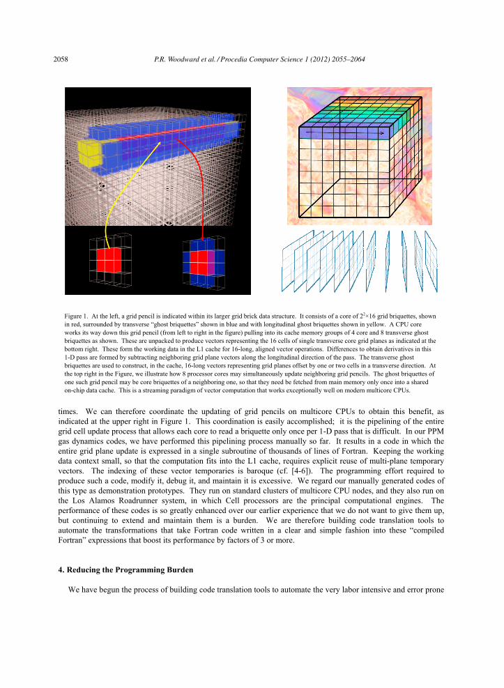
In Figure 2, we display results from runs carried out on our system to give an idea of the trade-offs between interactivity and resolution of flow detail in these two research problems. The multifluid mixing simulations shown on the top row in Figure 2 are the less challenging from this perspective. The three simulations shown are inspired by the Alpha Group study [9] of this problem. Our goal in this work is to carry out very highly resolved simulations whose output data we can mine to design and validate statistical models for subgrid-scale behavior in simulations involving this phenomenon. Clearly, such simulations cannot be carried out on our system in the LCSE but will instead require extremely large computing systems, like the petascale Roadrunner machine at Los Alamos. However, there are many issues in making these simulations that can be explored using our interactive system.

Figure 2. Examples of problems in two of our presently on-going research projects illustrating the trade-offs involved in balancing competing desires for interactive performance and for simulation detail. Along the top row of images, we see volume visualizations of the multifluid mixing fraction in a developing mixing layer as computed on grids of 1282×384, 2562×768, and 5122×1152 cells. In the bottom row of images, we see volume visualizations of the mixing fraction of entrained hydrogen fuel in the helium shell flash convection zone of an asymptotic giant branch (AGB) star of 2 solar masses using grids of 1923, 1923, and 5763 cells with heat injection rate multipliers of 64, 8, and 1 going from left to right. In the cases of both research projects, we give up fidelity to some extent in making the simulation run at interactive rates, but we gain enormously in our ability to rapidly scope out the fluid behaviour in a particular regime of parameter space, as discussed in the text. The flows at the left in both rows take only minutes to simulate, the flows in the center take around one hour, and, on our system, the flows at the right take half a day (top) and about 3 days (bottom). These simulations are discussed further in the text.



Among these issues are the dependence of the response of the mixing layer to different initial disturbance spectra, the effect of size of the domain as expressed in the importance of gas viscosity, and issues concerning alternative algorithmic methods for treating the multifluid fractional volume variable that is visualized in the three images in Figure 2. In these runs we are using a new technique to handle this fractional volume variable based upon the PPB (Piecewise-Parabolic Boltzmann) advection scheme [10,11]. The rapid response of our interactive system in the LCSE that we can achieve with our codes has been extremely helpful in establishing the proper ways in which to embed this moment-conserving advection scheme with our PPM gas dynamics calculation [1] in these problems. Rather than illustrate runs differing algorithmically here, we avoid the lengthy explanation of such alternative algorithms by focusing instead upon the simple effects of grid resolution for a single input spectrum.

The top row of images in Figure 2 shows three runs that use different grids and hence different amounts of time to arrive at the resulting flow states shown. From left to right we have 128, 256, and 512 grid cells across the problem domain. These problems are initialized in a fashion similar to that used in the Alpha Group study [9] of the turbulent mixing that results from the Rayleigh-Taylor instability at accelerated multifluid interfaces. We set the width of the periodic domain to 1, the acceleration due to gravity to -0.024, and the density contrast between the two fluids at the midplane to 3. We compute the flow as a perturbation to an initial background state that has hydrostatic equilibrium in the lighter fluid in the bottom half of the simulation, with a density at the midplane of unity and a sound speed there of unity, and hydrostatic equilibrium in the heavier fluid in the upper half of the simulation, with a density at the midplane of 3. Our unit of time in the problem is the time required for sound to cross the periodic domain at the midplane in the light fluid in the initial state. We begin with small amplitude displacements of the multifluid interface height that are made up of linear combinations of sinusoidal modes with randomly chosen relative strengths subject to the constraint that no modes with wavelengths longer than max=1/8 and none smaller than min=1/32 are included, and the average amplitude of a mode with 1 is larger than that of a mode with 2 by a factor ( 1/ 2)2 for the 2 flows at the left and a factor ( 1/ 2)3 for the flow at the right. The flows in the figure are shown at times 30, 30, and 34, going from left to right. The later time of the display for the flow at the right accounts for an approximate time offset that results from this simulation beginning with disturbance amplitudes that were smaller than in the other two runs by a factor of 1.6. Running at 4.5 Gflop/s/core on 192 CPU cores, the simulation at the left took about 4 minutes to reach the point shown in Figure 2. The simulation in the middle, due to its larger size, was a bit more efficient. Running at 5.6 Gflop/s/core on 192 cores, this run took just under one hour to reach the point shown. The simulation on the right, taking up much of the available memory on the system, ran at 5.0 Gflop/s/core on 192 cores and required about 10.5 hours to reach the point shown in Figure 2. These 3 runs therefore represent a progression from full interactive performance to an overnight calculation on our system.

There is fairly good agreement between all these three runs on the overall rate of spreading of the mixing layer, although a trend to a slightly lower rate with increasing grid resolution is evident. The left and center runs, which have identical initial disturbances, also serve to show the extent of detailed flow convergence one can expect for a 4-minute run on this system with our code. Clearly, the smaller wavelength modes have been strongly damped in this very rapid run on its coarse grid. This is not surprising, because the shortest wavelengths in the initial disturbance spectrum are “resolved” with only 4 grid cells. Runs of this speed on our system are most useful in testing new algorithmic approaches, which consumes a good deal of our time, and in rapidly getting a feel for the effects of changing simulation parameters such as the value of a Navier-Stokes viscosity. Runs like the one in the center in Figure 2 are also useful for more carefully assessing what we expect the output from much better resolved simula-tions to be, before we expend the effort to find out for certain. From this study of turbulent mixing, we plan to extract detailed information from runs we perform at very large scale on the Los Alamos Roadrunner machine. This information will be used to guide the design of subgrid-scale models for the turbulent mixing process. This use for the data demands highly accurate simulations involving very many modes and producing good statistical averages. Our interactive system is unsuitable for these large runs, but it has proved to be a tremendously useful tool in preparing to make such runs.

The bottom row of images in Figure 2 shows a more challenging application for our code and for the interactive computing system we have built in our lab. Here we are simulating the entrainment of stably stratified gas from above the helium shell flash convection zone in the deep interior of an asymptotic giant branch (AGB) star of 2 solar



masses (cf. [12-15]). Near the end of the life of such a star of extremely low metallicity (a first generation star), the star goes through a series of thermal pulses in which helium burning right above a degenerate core largely made of carbon alternates with hydrogen burning in a shell above this. The helium shell flash drives convection in a zone consisting largely of a helium-carbon mixture. As the convection zone grows with time, for a first-generation star it may reach a radius at which the unprocessed hydrogen-helium mixture begins. This unprocessed fuel is much more buoyant than the helium-carbon mixture of the convection zone, but nevertheless some of it can be entrained and brought downward to regions of such high temperature that it can burn very rapidly. We are working with Falk Herwig, at the University of Victoria, to simulate this process. The runs shown in the lower row of Figure 2 relate to this work.

The two runs at the left and center in the bottom row of Figure 2 both use grids of 1923 cells. The run at the right uses a grid of 5763 cells. This simulation code runs a bit faster than the version used for the Rayleigh-Taylor mixing simulations, but only by about 10 to 15%, since it does not utilize the transverse ghost briquettes indicated in blue in Figure 1. These fluid flow simulations pose greater challenges than those discussed earlier for three reasons: (1) the convection zone extends from about a radius of 10,000 km to about 30,000 km in the star’s central region, so only a fraction of the grid contains the region of interest, (2) the convection inside this zone involves modes that are global in scale, so we cannot use our grid to focus on just a portion of the convection zone, and (3) the gas entrainment requires high grid resolution in a very thin spherical surface at the top of the convection zone. The team of Arnett has been addressing these computational challenges, also using the PPM gas dynamics scheme, in the context of massive stars for many years (cf. [16]). In our study of the helium shell flash, we are not simply interested in a transient phenomenon, although compared to the life span of the star the two-year duration of the helium shell flash is very brief. However, in terms of the dynamical time scale for the star to readjust its radial structure via pressure waves or in terms of the convective eddy turnover time, we need to carry our simulation forward for an extensive period in order for the convection to become well established. In the flows shown at the left and center in Figure 2, we have sped up the flow dynamics in order to get a quick feel for its behavior. We accomplished this by multiply-ing the heat injection rate derived from 1-D stellar evolution calculations of Herwig [12] by factors of 64 (left) and 8 (center), while the run at the right has the correct heat injection rate. The indication from the images in Figure 2 is that the 64-fold heating enhancement, which causes the flow speeds to be roughly quadrupled, seems to change the character of the gas entrainment, while the 8-fold heating enhancement may not alter the flow character so much. The times required for the 3 simulations shown in the bottom row of Figure 2 are 13 minutes, 83 minutes, and 75 hours, and the flows are displayed at simulated times of 0.94 hours, and 6.27 hours for the other two runs. The run at the left is not carried as far forward in simulated time, because its much higher heat injection rate makes this unnecessary. We are just this year embarking on this study in earnest, and initial work reveals many interesting subtleties of these stellar convection flows. Despite the greater computing difficulty of these stellar astrophysical flows, our new interactive computing system is a major asset in this research.

The more challenging case of the helium shell flash simulations underscores the need to augment any system such as this with access to supercomputing systems. In collaboration with the Minnesota Sueprcomputing Institute, which has recently installed an HP computer with nodes similar to our Intel-based ones in the LCSE, but with 40 times as many of these, we are exploring the potential for scheduling interactive supercomputing events 2 days in advance. We have an Infiniband link to the MSI machine room running at 20 Gbit/s, which is sufficient to ship to our lab bursts of simulation data separated by about the 10 seconds required to process this data upon arrival into files that can be rendered into images and then to replicate the resulting files on all the nodes in the lab that cooperatively generate images for the PowerWall display. This mechanism can take us up in grid resolution by one additional factor of 2, which will make quite a difference for the stellar astrophysics simulations. We are also exploring the potential of GPUs for accelerating the LCSE system, so that it can deliver greater performance.

6. User Interface

In developing our interactive flow simulation capability, we have so far focused our greatest effort on the problem of simulation code performance. We will continue this effort as we explore the potential of GPU code accelerators. However, the 4-minute or 13-minute runs at the left in Figure 2 already place a strong demand on the



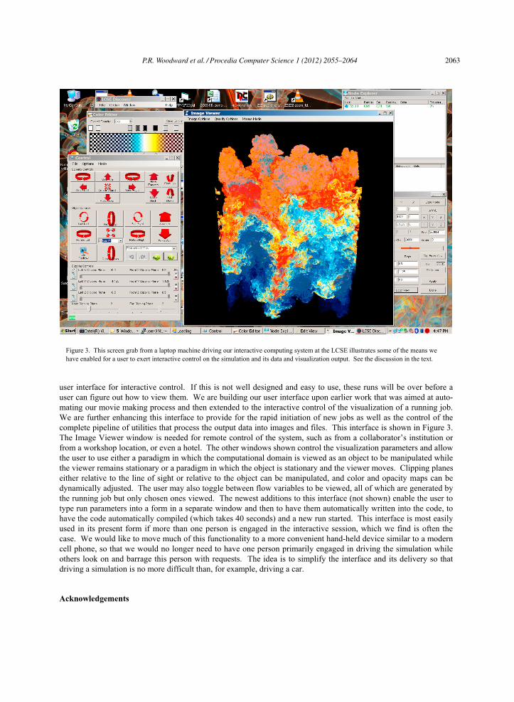
user interface for interactive control. If this is not well designed and easy to use, these runs will be over before a user can figure out how to view them. We are building our user interface upon earlier work that was aimed at auto-mating our movie making process and then extended to the interactive control of the visualization of a running job. We are further enhancing this interface to provide for the rapid initiation of new jobs as well as the control of the complete pipeline of utilities that process the output data into images and files. This interface is shown in Figure 3. The Image Viewer window is needed for remote control of the system, such as from a collaborator’s institution or from a workshop location, or even a hotel. The other windows shown control the visualization parameters and allow the user to use either a paradigm in which the computational domain is viewed as an object to be manipulated while the viewer remains stationary or a paradigm in which the object is stationary and the viewer moves. Clipping planes either relative to the line of sight or relative to the object can be manipulated, and color and opacity maps can be dynamically adjusted. The user may also toggle between flow variables to be viewed, all of which are generated by the running job but only chosen ones viewed. The newest additions to this interface (not shown) enable the user to type run parameters into a form in a separate window and then to have them automatically written into the code, to have the code automatically compiled (which takes 40 seconds) and a new run started. This interface is most easily used in its present form if more than one person is engaged in the interactive session, which we find is often the case. We would like to move much of this functionality to a more convenient hand-held device similar to a modern cell phone, so that we would no longer need to have one person primarily engaged in driving the simulation while others look on and barrage this person with requests. The idea is to simplify the interface and its delivery so that driving a simulation is no more difficult than, for example, driving a car.

Acknowledgements

Figure 3. This screen grab from a laptop machine driving our interactive computing system at the LCSE illustrates some of the means we have enabled for a user to exert interactive control on the simulation and its data and visualization output. See the discussion in the text.



We would like to acknowledge many helpful discussions over the course of this work with David Yuen and his research team as well as Tom Jones and his team. For our work with the Cell processor, we have interacted, mostly via E-mail, with Peter Hofstee of IBM, Austin, especially at the outset of the work. We are most grateful to Karl-Heinz Winkler at LANL for bringing the opportunity of the Cell processor to our attention and to the many experts on this technology at the Los Alamos National Laboratory who have interacted with us and encouraged our work with Cell and Roadrunner. We are particularly grateful to William Dai, of Los Alamos, for his continued interest and assistance in dealing with Roadrunner issues. Ben Bergen has also been very helpful in assisting us in getting started on the Roadrunner machine. The work we are doing on turbulent multifluid mixing is in close collaboration with Guy Dimonte, at Los Alamos, and the work on stellar convection involves close collaboration with Falk Herwig at the University of Victoria and Chris Fryer at LANL.

The construction and development of our interactive supercomputing system at the LCSE has been supported by an NSF Computer Research Infrastructure grant, CNS-0708822. Our work in interactive supercomputing has also been supported in part through the Minnesota Supercomputing Institute. Research work reported here as well as the development of our multifluid PPM gas dynamics code and translation tools for the Cell processor and Roadrunner system has been supported through a contract from the Los Alamos National Laboratory to the University of Minnesota.

References

1. P. R. Woodward, A Complete Description of the PPM Compressible Gas Dynamics Scheme. LCSE Internal Report. Available from the main LCSE page at: www.lcse.umn.edu; shorter version in Implicit Large Eddy Simulation: Computing Turbulent Fluid Dynamics, F. Grinstein, L. Margolin, and W. Rider (eds.). Cambridge University Press: Cambridge, 2006.

2. P. R. Woodward and D. H. Porter, PPM Code Kernel Performance. LCSE Internal Report. 2005. Available at: www.lcse.umn.edu. 3. P. R. Woodward and S. E. Anderson, Portable Petaflop/s Programming: Applying Distributed Computing Methodology to the Grid

within a Single Machine Room. Proceedings of the 8th IEEE International Conference on High Performance Distributed Computing,Redondo Beach, CA, August 1999. Available at www.lcse.umn.edu/HPDC8.

4. P. R. Woodward, J. Jayaraj, P.-H. Lin, and W. Dai, First experience of compressible gas dynamics simulation on the Los Alamos Roadrunner machine. Concurrency and Computation: Practice and Experience, 2009.

5. P. R. Woodward, J. Jayaraj, P.-H. Lin, and P.-C. Yew, Moving scientific codes to multicore microprocessor CPUs, Computing in Science and Engineering, Nov. 2008, 16-25.

6. P. R. Woodward, J. Jayaraj, P.-H. Lin, and D. Porter, Programming techniques for moving scientific simulation codes to Roadrunner. Tutorial given 3/12/09 at Los Alamos. Available at www.lanl.gov/roadrunner/rrtechnicalseminars2008.

7. T. Parr, The Definitive ANTLR Reference, Building Domain-Specific Languages, The Pragmatic Programmers, LLC, May, 2007. 8. Inertial Confinement Fusion: How to Make a Star. https://lasers.llnl.gov/programs/nic/icf/ 9. G. Dimonte et al. A comparative study of the turbulent Rayleigh-Taylor instability using high-resolution three-dimensional numerical

simulations: The Alpha-Group collaboration, Physics of Fluids 16, 1668-93, 2004. 10. P. R. Woodward, Numerical Methods for Astrophysicists, in Astrophysical Radiation Hydrodynamics, K.-H. Winkler and M. L. Norman

(eds.). Reidel: Dordrecht, 1986; 245–326. Available at: www.lcse.umn.edu/PPB. 11. P. R. Woodward, PPB, the Piecewise-Parabolic Boltzmann Scheme for Moment-Conserving Advection in 2 and 3 Dimensions. LCSE

Internal Report, 2005. Available at: www.lcse.umn.edu/PPBdocs. 12. F. Herwig, Evolution of Asymptotic Giant Branch Stars, Annual Reviews of Astronomy and Astrophysics 43, 435-79, 2005. 13. F. Herwig, B. Freytag, R. M. Hueckstaedt, and F. X. Timmes, Hydrodynamic Simulations of He Shell Flash Convection, Astrophysical

Journal 642, 1057–1074 (2006). 14. P. R. Woodward, F. Herwig, D. Porter, T. Fuchs, A. Nowatzki, and M. Pignatari. Nuclear Burning and Mixing in the First Stars:

Entrainment at a Convective Boundary using the PPB Advection Scheme, in First Stars III, eds. B. W. O’Shea, A. Heger, and T Abel, American Institute of Physics, 2008, p. 300-8.

15. P. R. Woodward, D. H. Porter, F. Herwig, M. Pignatari, J. Jayaraj, and P.-H. Lin. The hydrodynamic environment of the s-process in the He-shell flash of AGB stars. In Nuclei in the Cosmos (NIC X) (2008).

16. C. A. Meakin, and D. Arnett, ApJ Lett. 637, L53–L56 (2006).


Boosting the performance of computational fluid dynamics … · · 2017-01-18Paul R. Woodward, a*...

Documents

Transcript of Boosting the performance of computational fluid dynamics … · · 2017-01-18Paul R. Woodward, a*...