E

CON

OM

ÍA

S

N

SERIE DOCUMENTO

BBBOOORRRRRRAAADDDOOORRREEESSS

DDDEEE IIINNNVVVEEESSSTTTIIIGGGAAACCCIIIÓÓÓNNN

o. 17 Noviembre 2001

ISSN 0124-4396

ON THE DYNAMICS OF LENDING AND DEPOSIT INTEREST RATES IN EMERGING MARKETS: A NON-LINEAR APPROACH Ana María Iregui Costas Milas Jesús Otero

UNIVERSIDAD DEL ROSARIO

ON THE DYNAMICS OF LENDING AND DEPOSIT INTEREST RATES IN EMERGING MARKETS: A NON-LINEAR APPROACH ♦

Ana María Iregui♣

airegubo@banrep.gov.co

Costas Milas♣♣ c.k.milas@sheffield.ac.uk

Jesus Otero♣♣♣

jotero@claustro.urosario.edu.co

ABSTRACT

This paper studies the dynamics of lending and deposit rates in four emerging markets in Latin America: Argentina, Chile, Colombia and Mexico. The dynamics of interest rates exhibit a regime-switching behavior, where the transition from one regime to the other is controlled by the interest rate spread difference. The first regime, which is characterized by negative deviations of the interest rate spread relative to an estimated threshold, occurs during periods of financial liberalization. The second regime, which is characterized by positive deviations of the interest rate spread relative to the estimated threshold, occurs during periods of financial inefficiency and increasing government intervention. By capturing changing policy regimes from government intervention to a more financially liberalized environment and vice versa, the non-linear specification proves superior to the linear one.

RESUMEN Este trabajo estudia el comportamiento dinámico de las tasas de interés de captación y colocación en cuatro mercados emergentes en Latinoamérica: Argentina, Chile, Colombia y México. La dinámica de las tasas de interés muestra un comportamiento de cambio de régimen, donde la transición de un régimen a otro, es controlada por el diferencial entre las tasas. El primer régimen, caracterizado por desviaciones negativas del diferencial entre las tasas con respecto a un umbral estimado, ocurre durante periodos de liberalización financiera. El segundo, caracterizado por desviaciones positivas, ocurre durante periodos de ineficiencia financiera y creciente intervención. La especificación no lineal resulta mejor que la lineal en la medida en que permite capturar cambios de régimen.

Keywords: Interest rates; Spreads; Emerging markets, Non-linear models, Regimes JEL classification: C32; C51; C52; E43; O54

♦ The views expressed in this paper are those of the authors and do not represent those of the Board of Directors of the Banco de la República (Central Bank of Colombia), or other members of its staff. ♣ Estudios Económicos. Banco de la República. Bogotá, Colombia. ♣♣ Department of Economics. University of Sheffield. Sheffield, UK. ♣♣♣ Facultad de Economía. Universidad del Rosario. Bogotá, Colombia.

1

1. Introduction

The financial sector plays a crucial role in the operation of most economies, as it provides

intermediation between borrowers and lenders of funds. To the extent that financial

intermediaries are efficient institutions for channeling funds from savers to borrowers, they can

affect economic growth. The behavior of lending rates, deposit rates and their difference or

spread are key issues in the financial sector because they reflect the cost of intermediation. High

spreads are generally viewed as impediments to the development of the financial sector, since

they discourage potential savers with low returns on their deposits, and reduce the gross return of

potential investors.

The analysis of the main determinants of bank interest margins and profitability have been

topics of dynamic research in recent years; see for example Demirgüç-Kunt and Huizinga (1999),

the collection of case studies for a sample of Latin American countries in Brock and Rojas-

Suárez (2000), and the references therein. To our knowledge, however, less effort has been put on

the study of the determinants of the short- and long-run behavior of lending and deposit interest

rates. Understanding the dynamics of bank interest rates can help policymakers design measures

to overcome possible sources of inefficiency in financial markets and gain insight to the effects of

their policy measures.

The aim of this paper is to study the dynamic behavior of lending and deposit interest rates in

four emerging markets in Latin America. A priori there is reason to believe that lending and

deposit interest rates maintain a stable long-run equilibrium relationship, in the sense that these

variables exhibit a systematic co-movement over time. In the short run, however, equilibrium

may fail to hold because economies constantly experience shocks and other disturbances,

although economic forces do not allow for these short-run deviations from equilibrium to grow

indefinitely over time.

2

An interesting question that arises is that of the type of adjustment back to equilibrium, and in

particular the possibility of linear versus non-linear type of adjustments. Indeed, it is not at all

clear that interest rates respond symmetrically to positive and negative shocks, or to small and

large shocks. Interest rates, like other prices in the economy, may exhibit a tendency to increase

rapidly and reduce more gradually following a shock to the economy. A number of reasons could

potentially explain non-linear behavior in interest rates in emerging countries, including

government regulations in the form of interest rate controls, and non competitive environments

where strong banks may be more willing to increase rather than reduce their interest rates due to

their market power.

In this paper we aim to test for and model non-linearities in the lending and deposit interest

rates in four Latin American emerging markets: Argentina, Chile, Colombia, and Mexico. In

particular, we characterize the behavior of the interest rates using the Smooth Transition

Autoregressive (thereafter STAR) methodology. STAR models were originally introduced by

Teräsvirta and Anderson (1992) in order to examine non-linearities over the business cycle, and

their statistical properties were discussed in Granger and Teräsvirta (1993) and Teräsvirta (1994),

among others. In a recent survey of the STAR methodology and its applications, van Dijk et al.

(2000) point out that this form of non-linear models has mainly been applied to macroeconomic

time series and only recently to interest rate models in developed countries (see e.g. Anderson,

1997 for the US; van Dijk and Franses, 2000 for the Netherlands). To our knowledge, however,

the STAR methodology has not been applied so far to interest rate models in emerging market

economies.

The STAR model can be interpreted as a regime-switching model, where the transition from

one regime to the other occurs in a smooth way. At the same time, the transmission mechanism

between regimes is a function of the underlying explanatory variables. Modeling lending and

3

deposit interest rates in Latin America within the STAR context can be motivated by the fact that

the last decade has witnessed a transition period from repressed to more liberalized financial

environments. Assuming that the transition mechanism is controlled by the interest rate spread,

we can differentiate between the impact of the spread on lending and deposit interest rates during

periods of considerable impediment to the development of financial intermediation (when the

spread is too high), and its impact on lending and deposit rates during periods of increasing

competition (when the spread is low). Furthermore, we can identify threshold levels for the

spread rate that mark the transition from one regime to the other, as well as the speed at which

this transition takes place.

The outline of the paper is as follows. Section 2 provides a historical background to the

behavior of interest rates in Latin America. Section 3 introduces the theoretical aspects of non-

linear models in the context of the STAR methodology. Section 4 estimates linear and non-linear

models for the lending and deposit rates in Latin America. Section 5 presents a discussion of our

findings and section 6 provides some concluding remarks.

2. Historical context

For decades, Latin American economies pursued inward-looking development strategies in

which government intervention was predominant. Consequently, these economies were

characterized by the use of trade barriers and foreign exchange controls to protect indigenous

infant industries against foreign competition, and by heavily controlled financial systems that

resulted in financial repression. Financial repression is a term that refers to a policy regime in

which high reserve requirements are imposed on financial intermediaries as well as ceilings on

their deposit and lending interest rates. In addition to these features, there are restrictions on

competition in the banking industry and on the composition of bank portfolios. The former takes

the form of entry barriers into the banking system and public ownership of financial institutions;

4

the latter consists of the operation of non-price mechanisms of credit allocation in the form of

directed lending to specific productive sectors (Agénor and Montiel, 1996).

During the second half of the 1970s, the Southern cone economies of Argentina, Chile and

Uruguay implemented market-oriented reforms in an attempt to improve resource allocation

within a more financially liberalized environment. As indicated by Corbo et al. (1986),

liberalization measures in these countries included the removal of interest rate controls. However,

this policy measure proved to be unsuccessful mainly due to the fact that governments, either

explicitly or implicitly, provided deposit insurance at no cost. As a result, central banks and the

rest of the public sector had to intervene to rescue institutions facing financial difficulties. For

instance, Chile faced a banking crisis in the early 1980s, which, during the restructuring process,

required financial aid to the banking system of around 20 percent of the country’s GDP (see e.g.

Rojas-Suárez and Wiesbrod, 1996). According to Corbo et al. (1986), governments could have

avoided moral hazard problems by refusing to provide free deposit insurance to failed

intermediaries and by creating an effective system of regulation and supervision of the loan

portfolios of financial intermediaries.

In fact, the 1980s were characterized by financial repression. For instance, following the debt

crisis of 1982 in Mexico, all Mexican banks were nationalized, and the government imposed high

reserve requirements, set ceilings on interest rates, and directed lending to specific “high priority”

productive sectors (Saunders and Schumacher, 2000). Colombia entered the 1980s facing the

collapse of coffee prices (i.e. the country’s main export product and an important determinant of

its business cycle), along with a deteriorating situation of government finances. Montenegro

(1983) argues that the financial crisis of the early 1980s can be explained, to a great extent, by

this economic downturn. The crisis hit strongly poorly capitalized banks as well as small banks,

all of which suffered from loan portfolios concentrated on unprofitable firms often belonging to

the owners of the banks. This last aspect also reflects a system where the operations of financial

5

intermediaries were not properly supervised and regulated by the authorities. 1

During the 1990s, Latin American economies adopted policy reforms aimed at providing a

transition to a more liberalized domestic financial sector. As indicated by Brock and Suárez-

Rojas (2000), the liberalization process was tested in two occasions. The first one during the

Mexican financial turmoil of 1995 and the second one during the eruption of the severe financial

crisis that hit the Asian economies in mid 1997 followed by global economic uncertainties in

response to the Russian moratorium in mid 1998. As Brock and Suárez-Rojas (2000) point out,

Latin American authorities responded to the financial crises of the 1990s by intensifying their

efforts for deeper reforms, rather than turning back to government intervention policies that

followed the failure of liberalization measures in the second half of the 1970s.

The discussion so far points to changing policy regimes from government intervention to a

more financially liberalized environment in the banking industry of the Latin American

economies. The next section of the paper discusses the theory of regime-switching models in the

context of the STAR methodology that will be empirically tested on the behavior of lending and

deposit interest rates in the Latin American economies.

3. Specification of STAR models

The STAR model of order k for a univariate time series yt is written as:

1 In Colombia, banks were also subject to high rates of financial taxation, which provided an additional factor of financial repression. A description of the institutional background in the Colombian financial sector can be found in Barajas et al. (1999, 2000).

,,...,1,)())(1(1

,221

,11 TtsGysGyy tdt

k

jjtjdt

k

jjtjt =ε+

β+µ+−

β+µ= −

=−−

=− ∑∑ (1)

6

where µ1 and µ1 are intercept terms and εt ~ iid (0, σ2). G(st−d) is the transition function, which is

assumed to be continuous and bounded between zero and one, and d is the delay parameter. The

STAR model (1) can be considered as a regime-switching model which allows for two regimes,

G(st−d) = 0 and G(st−d) = 1, respectively, where the transition from one to the other regime occurs

in a smooth way. The regime that occurs at time t is determined by the transition variable st−d and

the corresponding value of G(st−d). Different functional forms of G(st−d) allow for different types

of regime-switching behavior. In particular, asymmetric adjustment to positive and negative

deviations of st−d relative to a parameter c, can be obtained by setting G(st−d) equal to the

‘logistic’ function:

(2a)

where σ(st−d) is the sample standard deviation of st−d. The parameter c is the threshold between

the two regimes, in the sense that G(st−d) changes monotonically from 0 to 1 as st−d increases,

while G(st−d) = 0.5. The parameter γ determines the smoothness of the change in the value of the

logistic function and thus the speed of the transition from one regime to the other. When 0→γ ,

the ‘logistic’ function equals a constant (i.e. 0.5), and when ∞→γ , the transition from

G(st−d) = 0 to G(st−d) = 1 is almost instantaneous at st−d = c.

Another type of regime-switching behavior, which describes asymmetric adjustment to small

and large absolute values of st−d, is obtained by setting G(st−d) equal to the ‘exponential’ function:

A possible drawback of the ‘exponential’ function is that the model becomes linear if either

0→γ or ∞→γ . To overcome this drawback, Jansen and Teräsvirta (1996) suggest specifying

,0,)]}(/)(exp[1{),;( 1 >γσ−γ−+=γ −−−− dtdtdt scscsG

.0)},(/)(exp{1),;( 22 >γσ−γ−−=γ −−− dtdtdt scscsG

7

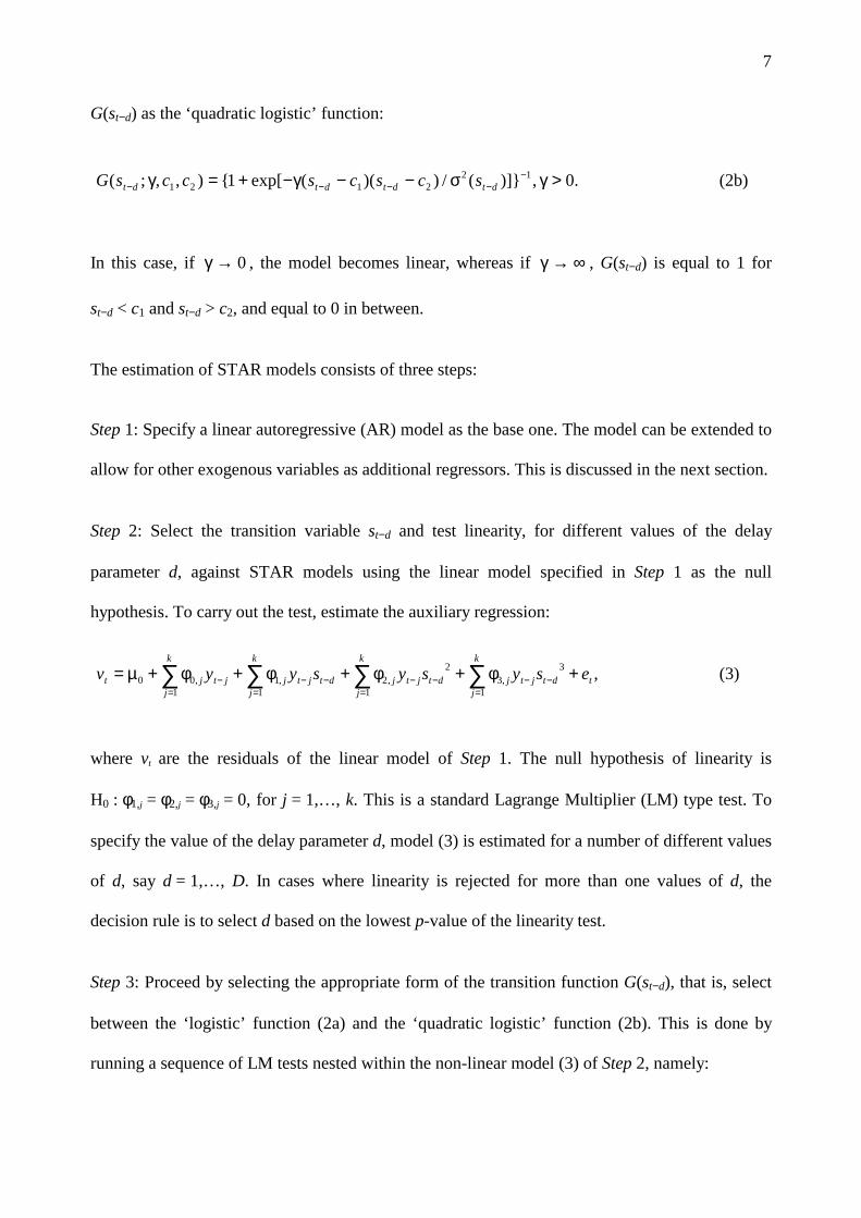
G(st−d) as the ‘quadratic logistic’ function:

In this case, if 0→γ , the model becomes linear, whereas if ∞→γ , G(st−d) is equal to 1 for

st−d < c1 and st−d > c2, and equal to 0 in between.

The estimation of STAR models consists of three steps:

Step 1: Specify a linear autoregressive (AR) model as the base one. The model can be extended to

allow for other exogenous variables as additional regressors. This is discussed in the next section.

Step 2: Select the transition variable st−d and test linearity, for different values of the delay

parameter d, against STAR models using the linear model specified in Step 1 as the null

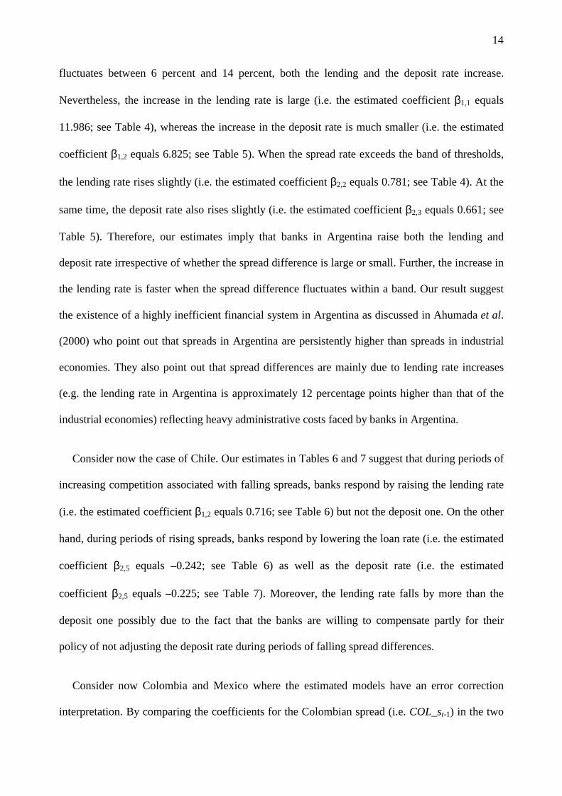
hypothesis. To carry out the test, estimate the auxiliary regression:

where vt are the residuals of the linear model of Step 1. The null hypothesis of linearity is

H0 : φ1,j = φ2,j = φ3,j = 0, for j = 1,…, k. This is a standard Lagrange Multiplier (LM) type test. To

specify the value of the delay parameter d, model (3) is estimated for a number of different values

of d, say d = 1,…, D. In cases where linearity is rejected for more than one values of d, the

decision rule is to select d based on the lowest p-value of the linearity test.

Step 3: Proceed by selecting the appropriate form of the transition function G(st−d), that is, select

between the ‘logistic’ function (2a) and the ‘quadratic logistic’ function (2b). This is done by

running a sequence of LM tests nested within the non-linear model (3) of Step 2, namely:

.0,)]}(/))((exp[1{),,;( 122121 >γσ−−γ−+=γ −

−−−− dtdtdtdt scscsccsG (2b)

,1 1

3,3

2,2

1,1

1,00 ∑ ∑∑∑

= =−−−−

=−−

=− +φ+φ+φ+φ+µ=

k

jt

k

jdtjtjdtjtj

k

jdtjtj

k

jjtjt esysysyyv (3)

8

.0|0:,0|0:

,0:

,2,3,101

,3,202

,303

=φ=φ=φΗ

=φ=φΗ

=φΗ

jjj

jj

j

(4)

In this case, the decision rule is to select the ‘quadratic logistic’ function (2b) if the p-value

associated with the Η02 hypothesis is the smallest one, otherwise select the ‘logistic’ function

(2a). Having done that, proceed by estimating the STAR model (1), with the transition function

G(st−d) specified based on the sequence of tests in (4).

4. Empirical results

4.1 The data

We use monthly data on the lending and deposit interest rates for four emerging markets in

Latin America. The countries are Argentina, Chile, Colombia and Mexico. The data set is

obtained from the IMF International Financial Statistics database. Data for Argentina is from

1993:M4 to 2000:M3. Data for Chile is from 1977:M1 to 2000:M3. Colombian data is from

1986:M1 to 2000:M3 and Mexican data is from 1993:M1 to 2000:M3. The sample choice is

dictated by the availability of data in the IMF database.

Figure 1 plots the levels of the interest rates for the four emerging market economies. We also

plot the interest rate spreads constructed as the difference between the lending and the deposit

interest rates for each of the four emerging markets.

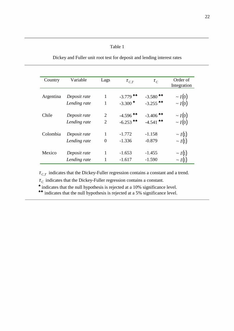
Estimation of linear and non-linear models requires stationarity of the interest rate series.

Table 1 reports the Augmented Dickey Fuller (ADF) tests on the levels and the first differences

9

of the series. ADF tests are also reported for the interest rate spreads. The results suggest that

Colombian and Mexican interest rates are non-stationary (i.e. I(1)) in levels, whereas the interest

rates for Argentina and Chile are stationary (i.e. I(0)) in levels. The spreads are found to be

stationary for all countries. Based on the results of the unit root tests, linear and non-linear

models are estimated for the levels of the interest rates in Argentina and Chile and for the first

differences of the interest rates in Colombia and Mexico. 2

In the remaining of the paper we adopt the following notation for the interest rate series in the

four emerging markets: lending, deposit and spread rates in Argentina are denoted by ARG_l,

ARG_d and ARG_s, respectively. CHI_l, CHI_d and CHI_s refer to the corresponding series in

Chile. COL_l, COL_d and COL_s refer to the corresponding series in Colombia and MEX_l,

MEX_d and MEX_s refer to the corresponding series in Mexico.

4.2 Testing for linearity and STAR model selection

As discussed in section 3, the first step in deriving STAR models involves the estimation of

linear interest rate models. These are reported in Table 2 (all estimations are done in PcGive, see

Hendry and Doornik, 1997). In deriving parsimonious linear models we apply the general-to-

specific approach starting with k = 12 lags on the lending and deposit rates and deleting all

insignificant variables. Our results suggest a feedback from deposit rates on lending rates and

vice versa. We also find significant lagged interest rate spread effects.

In the case of Colombia and Mexico (see Table 2E and Table 2F, respectively), the interest

rate equations can be interpreted as error correction models; lending interest rate changes react to

the disequilibrium error given by the lagged interest rate spread. 3 The coefficient on the lagged

2 Phillips-Perron tests give similar unit root results and are available by the authors on request. 3 Due to the small sample, some caution is needed when interpreting the Mexican interest rate equation as an error correction model.

10

spread is estimated at –0.394 for Colombia and at –0.126 for Mexico.

Notice also that no deposit rate equations are reported for Colombia and Mexico. The reason is

that we were unable to find any significant effect from the lending rates or the lagged interest rate

spreads in the deposit rate equations. This result points to weak exogeneity of the deposit rates. A

possible economic explanation for this finding is that at least in Colombia and Mexico, financial

liberalization has given domestic residents the opportunity to rebalance their portfolios

internationally, achieving a convergence of domestic deposit rates (adjusted for expectations of

exchange rate changes) towards international rates. On the other hand, convergence of domestic

and international lending rates is less likely to occur due to information costs associated with

monitoring domestic borrowers. As a result, international capital markets do not lend directly to

companies, rather, foreign lending is intermediated by domestic banks.4

The diagnostic tests of the linear models in Table 2 show some weak evidence (at the 5

percent level of statistical significance) of autocorrelation of up to order 12 for the deposit rate in

Argentina (see Table 2B) and the two interest rate models in Chile (see Table 2C and Table 2D,

respectively). ARCH effects of order 12 are reported for the lending rate in Colombia (see Table

2E), and the two interest rate models in Chile (see Table 2C and Table 2D, respectively). All

interest rate models fail normality. The failure of the diagnostic tests in the linear models

provides a further motivation for considering the possibility that the interest rates in the four

emerging economies might be better characterized by a non-linear type of behavior rather than

the linear one discussed above.

Having estimated the base linear models, we move on to Step 2 of our methodology which

4 A similar argument is put forward by Brock and Rojas-Suarez (2000). They motivate their discussion on the grounds of a low correlation coefficient between deposit rates and interest rate spreads for six Latin American economies (i.e. Argentina, Bolivia, Chile, Colombia, Mexico, Peru, and Uruguay) using quarterly data over the 1991-1996 period.

11

involves testing for the existence of non-linear dynamics in the lending and deposit interest rate

models for the four Latin American economies selecting the interest rate spread as a possible

transition variable st-d.

The empirical results of the LM-type tests for linearity (Steps 2 and 3 of section 3) are reported

in Table 3. We set d equal to 1 through 6 (although the results are not affected even if we go up to

12=d ). Using 0.01 as a threshold p-value, one can notice from Table 3A that the null hypothesis

of linearity, (that is, H0) is rejected for all models. The H0 hypothesis is rejected most strongly at

d = 1 for Colombia and the deposit rate models in Argentina and Chile, respectively. The results

also suggest a choice of d = 2 for Mexico, d = 3 for the lending rate in Argentina, and d = 5 for

the lending rate in Chile. Given the above choices, one can notice from Table 3B that the

sequence of tests (H03, H02, and H01, respectively) favor the ‘logistic’ model (2a) as the

appropriate transition function.

4.3 Estimates of the non-linear models

We estimate the STAR model (1) using the ‘logistic’ model (2a) by non-linear least squares

(NLS). Granger and Teräsvirta (1993) and Teräsvirta (1994) stress particular problems like slow

convergence or overestimation associated with estimates of the γ parameter. For this reason, we

follow their suggestions in standardizing the exponent of the ‘logistic’ function (2a) by dividing it

by the standard deviation of the transition variable, σ(st−d) so that γ becomes a scale-free

parameter. Based on this scaling, we use γ = 1 as the starting value and the mean of st−d as the

starting value for the parameter c. The estimates of the parsimonious linear interest rate equations

in Table 2 are used as starting values for the other parameters in the STAR model (1).

Tables 4 to 9 report the NLS estimates of the parsimonious STAR interest rate models. Before

interpreting our empirical results, it should be pointed out that our attempts to fit non-linear

12

models for the interest rates in Argentina based on the ‘logistic’ model (2a) resulted in

insignificant estimates. For this reason, we report non-linear models based on the ‘quadratic

logistic’ function (2b) which was found to work much better than the ‘logistic’ one. 5

The main parameters of interest in the STAR models are the estimated values of the threshold

level, c, and the speed of adjustment, γ. The c estimates reported in Tables 4 to 9 are statistically

significant in all models except for the deposit rate model in Chile (see Table 7), whereas the

estimates of the γ parameter are rather high for all models indicating that the speed of the

transition from G(st-d; γ, c) = 0 to G(st-d; γ, c) = 1 is rapid at the estimated threshold c. Notice,

however, the rather high standard error of the γ estimates. Teräsvirta (1994) and van Dijk et al.

(2000) point out that this should not be interpreted as evidence of weak non-linearity. Accurate

estimation of γ might be difficult as it requires many observations in the immediate neighborhood

of the threshold c. Further, large changes in γ have only a small effect on the shape of the

transition function implying that high accuracy in estimating γ is not necessary (see the

discussion in van Dijk et al., 2000).

From Tables 4 to 9 one can see that the error variance ratio of the non-linear relative to the

linear models (i.e. s2NL/s2

L) is less than one, indicating that the non-linear models have a better fit.

In particular, the s2NL/s2

L ratio shows a reduction in the residual variances of the non-linear

compared to the linear models which ranges from around 3 percent for the lending rate in Chile

(i.e. the CHI_lt model in Table 6) to 52 percent for the deposit rate in Argentina (i.e. the ARG_dt

model in Table 5). In addition, the non-linear specification captures the autocorrelation effects

that are present in the linear specification of the deposit rate in Argentina and the two interest rate

5 In the empirical results below, we estimate the ‘quadratic logistic’ model for the lending rate in Argentina using d = 1 rather than d = 3. This is done because the empirical model is found to work better for d = 1. We do not see this as a serious deviation from choosing d values based on the lowest p-value of the H0 hypothesis; one can see from Table 3A that there is little difference between p-value = 0.000341 for d = 3, and p-value = 0.000554 for d = 1.

13

models in Chile. It also captures the ARCH effects that are present in the linear interest rate

model for Colombia, and some of the ARCH effects in the two linear interest rate models for

Chile. There is also a considerable improvement in the test for normality although the test still

fails for all models.

5. Interpretation of results

Our research identified the existence of non-linear dynamics in the behavior of the lending and

deposit interest rates for four emerging markets in Latin America. Moreover, these interest rates

exhibit a regime-switching behavior according to the variation of the interest rate spread. The

result confirms the importance of the spread rate as a factor affecting the evolution of the lending

and deposit rates. Furthermore, the regimes we identify have a plausible economic interpretation.

The first regime (i.e. G(st-d; γ, c) = 0), which is defined by negative values of the interest rate

spread relative to a threshold, is usually identified with periods of financial liberalization and

modernization of the banking system which promotes competition within the banking sector.

Conversely, the second regime (i.e. G(st-d; γ, c) = 1), which is defined by positive values of the

interest rate spread relative to the threshold, is usually identified with periods of inefficiency in

banking activities which in turn adversely affect domestic savings and investments.

Our estimates in Tables 4-9 allow for the behavior of the interest rate spread to vary across

regimes for the four emerging market economies. Tables 4 and 5 report the non-linear estimates

for the lending and deposit rates in Argentina, respectively. One can notice that the threshold

estimates are roughly the same for both interest rate equations. Use of the ‘quadratic logistic’

function allows for the two regimes to be defined as follows; the first one (i.e. G(st-d; γ, c1,

c2) = 0) in terms of small values of the interest rate spread and the second one (i.e. G(st-d; γ, c1,

c2) = 1) in terms of large values of the interest rate spread. When the interest rate spread

14

fluctuates between 6 percent and 14 percent, both the lending and the deposit rate increase.

Nevertheless, the increase in the lending rate is large (i.e. the estimated coefficient β1,1 equals

11.986; see Table 4), whereas the increase in the deposit rate is much smaller (i.e. the estimated

coefficient β1,2 equals 6.825; see Table 5). When the spread rate exceeds the band of thresholds,

the lending rate rises slightly (i.e. the estimated coefficient β2,2 equals 0.781; see Table 4). At the

same time, the deposit rate also rises slightly (i.e. the estimated coefficient β2,3 equals 0.661; see

Table 5). Therefore, our estimates imply that banks in Argentina raise both the lending and

deposit rate irrespective of whether the spread difference is large or small. Further, the increase in

the lending rate is faster when the spread difference fluctuates within a band. Our result suggest

the existence of a highly inefficient financial system in Argentina as discussed in Ahumada et al.

(2000) who point out that spreads in Argentina are persistently higher than spreads in industrial

economies. They also point out that spread differences are mainly due to lending rate increases

(e.g. the lending rate in Argentina is approximately 12 percentage points higher than that of the

industrial economies) reflecting heavy administrative costs faced by banks in Argentina.

Consider now the case of Chile. Our estimates in Tables 6 and 7 suggest that during periods of

increasing competition associated with falling spreads, banks respond by raising the lending rate

(i.e. the estimated coefficient β1,2 equals 0.716; see Table 6) but not the deposit one. On the other

hand, during periods of rising spreads, banks respond by lowering the loan rate (i.e. the estimated

coefficient β2,5 equals –0.242; see Table 6) as well as the deposit rate (i.e. the estimated

coefficient β2,5 equals –0.225; see Table 7). Moreover, the lending rate falls by more than the

deposit one possibly due to the fact that the banks are willing to compensate partly for their

policy of not adjusting the deposit rate during periods of falling spread differences.

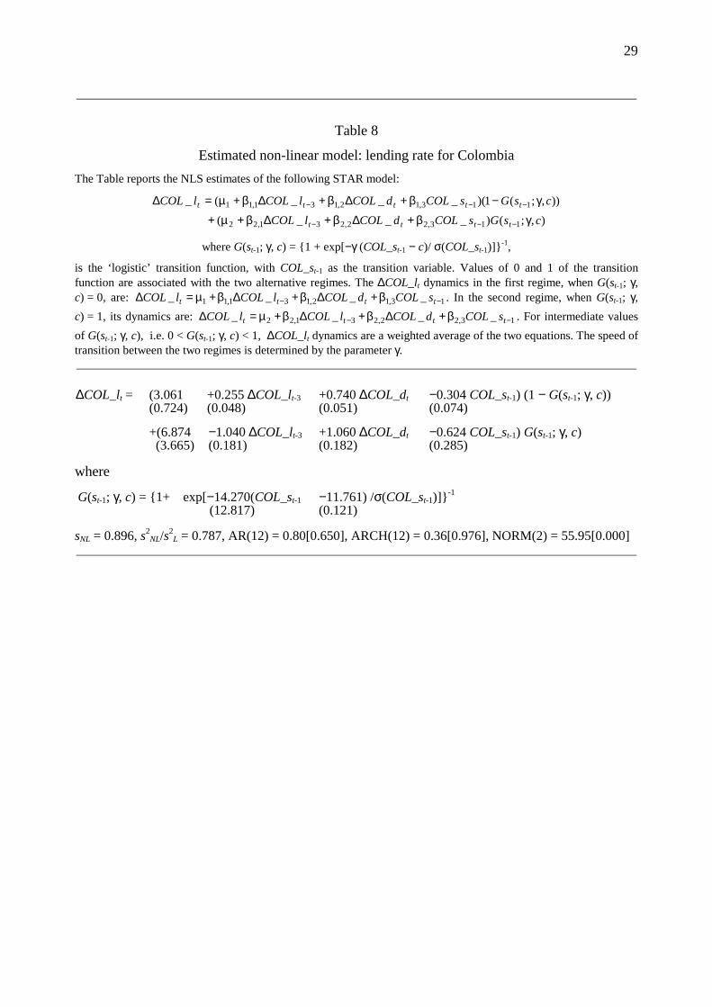
Consider now Colombia and Mexico where the estimated models have an error correction

interpretation. By comparing the coefficients for the Colombian spread (i.e. COL_st-1) in the two

15

regimes (i.e. the coefficients β1,3 and β2,3, respectively; see Table 8) we see that during periods of

banking competition (when the lagged spread is below the threshold level of 11.8 percent), the

lending interest rate adjusts slowly (i.e. the estimated coefficient β1,3 equals –0.304). On the other

hand, during periods of banking inefficiency (when the lagged spread is above 11.8 percent), the

lending interest rate adjusts much faster (i.e. the estimated coefficient β2,3 equals –0.624). The

results for Mexico in Table 9 point to a fast adjustment of the lending interest rate during periods

of banking inefficiency when the Mexican spread (i.e. MEX_st-2) is above 24 percent (i.e. the

estimated coefficient β2,4 equals –1.738). On the other hand, the lending interest rate does not

respond to spread values below its equilibrium level.

Our estimates for Colombia and Mexico suggest that a spread increase above its equilibrium

level is followed by temporary market share losses. To regain their market shares, banks have the

option of either lowering loan rates and/or raising deposit rates. Nevertheless, taking into account

that domestic deposit rates are somewhat outside the banks’ control in the sense that they move in

line with international deposit rates, it is not surprising that banks respond by lowering lending

rates rapidly in order to restore market shares.

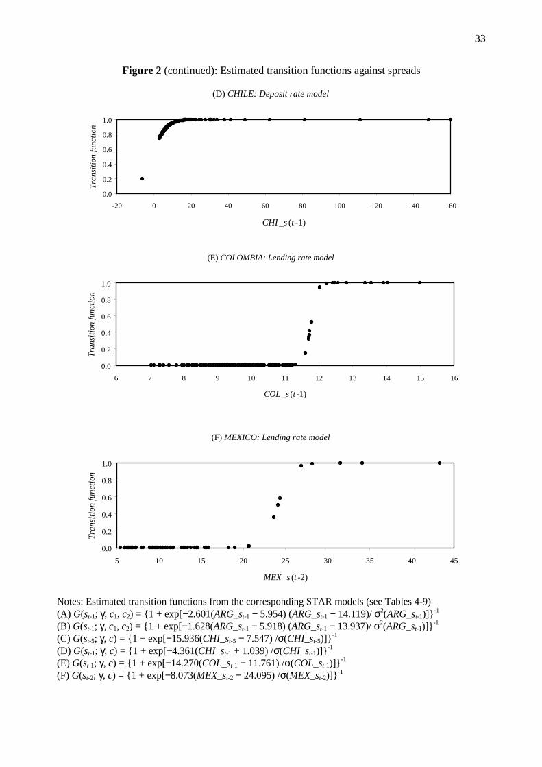
The relationship between the occurrence of a regime and the interest rate spread is depicted in

Figure 2, which plots the values of the estimated transition function against the spread for the

four Latin American economies. As discussed above, values of zero and one of the transition

function are related to the occurrence of the first regime (that is, periods of financial

liberalization) and the second regime (that is, periods of extensive government intervention and

financial inefficiency), respectively. In addition, this Figure helps clarify the discussion about the

speed of transition between the two regimes. One can see that the transition from one regime to

the other is rapid, as the estimates of γ are rather high for all models.

16

Figure 3 plots the estimated transition functions against time in order to illustrate the

succession of the regimes over the sample period. In the case of Argentina, the estimated

transition function classifies most of the sample period into the second regime, which points to

the existence of a highly inefficient financial system. Our findings are in line with the results

obtained by Ahumada et al. (2000), in the sense that the Argentine financial system is

characterized by persistently high lending interest rates resulting from high administrative costs.

In the case of Chile, the plots of the estimated transition functions for both the lending and

deposit rate models suggest that intermediate regimes are predominant most of the time. The

estimated transition functions against time classify the 1982-1983 financial crisis into the second

regime of financial inefficiency and government intervention aiming at disinflation policies in the

form of a prolonged exchange rate overvaluation and high interest rates (see e.g. the discussion in

Gavin and Hausmann, 1996).

The estimated transition functions for Colombia and Mexico reflect the financial liberalization

efforts taking place in these countries. In the case of Colombia, the estimated transition function

classifies most of the sample period into the first regime which is consistent with the

liberalization efforts taking place after the mid 1980s. Movements to the second regime around

1994-1996 might be explained by the tight monetary policy implemented by the Central Bank in

order to reduce inflationary pressures, which resulted in high interest rates. Classification of late

1998 into the second regime reflects high interest rates as the result of the government financing

its budget deficit by issuing bonds in the domestic market. It could also be related to the adverse

effects of two successive external shocks. The first one was related to the negative income effect

generated by the deterioration in the terms of trade. Terms of trade deteriorated following a

reduction in the international prices of primary commodities that resulted from the economic

crisis in the South East Asian economies. The second external shock was caused by the Russian

17

declaration of moratorium of its foreign debt. Thus, Colombia not only suffered from an income

reduction due to adverse international conditions, but also from a reduction in the availability of

resources in foreign markets as well as an increase in the cost of its foreign debt and a reduction

in foreign investment.

In the case of Mexico, classification of the beginning of 1995 into the second regime reflects

the profound financial crisis of that period. Classification of late 1998 and early 1999 into the

second regime probably reflects the economic downturn in South East Asia as well as the

financial instability following the Russian crisis, and the subsequent collapse of the Long Term

Capital Management (LTCM) hedge fund. Financial and economic instability had an adverse

effect on the expectations of foreign investors resulting in a reduction of capital flows towards

Mexico and other Latin American economies.

Taking into account that the Latin American economies have often suffered by severe banking

crises, it is interesting to compare the stability of the estimated linear and non-linear models using

recursive estimates. Figures 4 to 7 plot the 1-step residuals ± 2*standard errors and the N↑ step

Chow tests together with their 1% critical values for the linear and the non-linear models in the four

Latin American economies (for a detailed discussion of these tests see Hendry and Doornik, 1997).

The plots of the 1-step residuals ± 2*standard errors do not indicate significant differences between

the linear and the non-linear models. However, the N↑ step Chow tests indicate that the non-linear

are much more parameter stable compared to the linear ones. This result is more evident for the

deposit rate in Argentina (compare bottom left with bottom right panel in Figure 4B) and the lending

rate in Mexico (compare bottom left with bottom right panel in Figure 7). Parameter stability does

not improve for the deposit rate in Chile (compare bottom left with bottom right panel in Figure 5B)

where we could not get a significant estimate for the threshold parameter (see Table 7). The

recursive tests suggest an improvement in the parameter stability of the estimated models by taking

18

into account regime-switching behavior.

6. Conclusions

In this paper we model the dynamic behavior of lending and deposit interest rates in four Latin

American emerging markets using the smooth transition regime-switching framework. This

specification seems to work well both in statistical and economic terms. In statistical terms, it

captures most of the diagnostic test failures of the linear models. In economic terms, it provides a

plausible economic explanation of the alternative regimes. According to our results, the dynamics

of interest rates exhibit a regime-switching behavior, where the transition from one regime to the

other is controlled by the interest rate spread. The first regime, which is characterized by negative

values of the interest rate spread relative to a threshold, occurs during periods of financial

liberalization and modernization of the banking system. The second regime, which is

characterized by positive values of the interest rate spread relative to the threshold, occurs during

periods of inefficiency in banking activities and increasing government regulations.

Our results provide evidence that domestic deposit rates in Latin America move in line with

international deposit rates. This is probably due to the fact that financial liberalization allows

domestic residents to rebalance their portfolios internationally, achieving a convergence of

domestic deposit rates towards international rates. From the four emerging market economies

considered in this paper, the above finding is more evident in Colombia and Mexico. As domestic

deposit rates are somewhat outside the banks’ control in the sense that they converge to

international deposit rates, banks in Colombia and Mexico face temporary market share losses

when large spread differences occur. To restore market shares, banks respond by lowering

lending rates rapidly and this implies that periods of large spread differences are only short-lived.

On the other hand, financial liberalization efforts are less evident in Argentina. The estimates of

the regime-switching model suggest not only that banks in Argentina raise both the lending and

19

deposit rate (irrespective of whether the spread difference is large or small) but also that the

increase in the lending rate is larger than that of the deposit one.

So far, the smooth transition regime-switching specification has mainly been applied to

macroeconomic time series. Encouraged by our results for the dynamics of lending and deposit

interest rates in Latin America, we view the incorporation of smooth transition models to interest

rates and other finance applications as a promising area of future research.

20

References

Agénor, P.R. and P.J. Montiel, 1996. Development Macroeconomics. Princeton University Press,

Princeton.

Ahumada, H., T. Burdisso, J.P. Nicolini, and A. Powell, 2000. Spreads in the Argentine financial

system, in P.L. Brock and L. Suárez-Rojas (Eds.), Why so high? Understanding interest rate

spreads in Latin America. Inter-American Development Bank, Washington, 39-65.

Anderson, H.M., 1997. Transaction costs and nonlinear adjustment towards equilibrium in the US

Treasury Bill market, Oxford Bulletin of Economics and Statistics 59, 465-484.

Barajas, A., R. Steiner, and N. Salazar, 1999. Interest spreads in banking in Colombia, 1974-

1996, IMF Staff Papers 46, 196-224.

Barajas, A., R. Steiner, and N. Salazar, 2000. The impact of liberalization and foreign investment

in Colombia's financial sector, Journal of Development Economics 63, 157-196.

Brock, P.L. and L. Rojas-Suárez, 2000, Interest rate spreads in Latin America: Facts, theories,

and policy recommendations, in P.L. Brock and L. Suárez-Rojas (Eds.),Why so high?

Understanding interest rate spreads in Latin America. Inter-American Development Bank,

Washington.

Corbo, V., J. De Melo, and J. Tybout, 1986. What went wrong with the recent reforms in the

Southern cone, Economic Development and Cultural Change 34, 607-640.

Demirgüç-Kunt, A. and H. Huizinga, 1999. Determinants of commercial banks interest margins

and profitability: Some international evidence, The World Bank Economic Review 13, 379-

408.

Gavin, M. and R. Hausmann, 1996. The roots of banking crises: the macroeconomic context,

Inter-American Development Bank, Washington, Working paper No. 318.

Granger, C.W.J. and T. Teräsvirta, 1993. Modelling nonlinear economic relationships, Oxford

University Press, Oxford.

21

Hendry, D.F. and J.A. Doornik, 1997. Modelling Dynamic Systems Using PcFiml 9.0 for

Windows, London: International Thomson Business Press.

Jansen, E.S. and T. Teräsvirta, 1996. Testing parameter constancy and super exogeneity in

econometric equations, Oxford Bulletin of Economics and Statistics 58, 735-768.

Levine, R., 1997. Financial development and economic growth, Journal of Economic Literature

35, 688-726.

Montenegro, A., 1983. La crisis del sector financiero Colombiano, Ensayos Sobre Política

Económica 4, 51-89.

Rojas-Suárez, L. and S. Wiesbrod, 1996. Building stability in Latin American financial markets,

Inter-American Development Bank, Washington, Working paper No. 320.

Saunders, A. and L. Schumacher, 2000. The determinants of bank interest rate margins in

Mexico's postprivatisation period (1992-95), in P.L. Brock and L. Suárez-Rojas (Eds.), Why so

high? Understanding interest rate spreads in Latin America. Inter-American Development

Bank, Washington, 181-209.

Teräsvirta, T., 1994. Specification, estimation, and evaluation of smooth transition autoregressive

models, Journal of the American Statistical Association 89, 208-218.

Teräsvirta, T. and H.M. Anderson, 1992. Characterizing nonlinearities in business cycles using

smooth transition autoregressive models, Journal of Applied Econometrics 7, S119-S136.

van Dijk, D., and P.H. Franses, 2000. Nonlinear error-correction models for interest rates in the

Netherlands, in W.A. Barnett, D.F. Hendry, S. Hylleberg, T. Teräsvirta, D. Tjøstheim and A.

Würtz (Eds.), Nonlinear econometric modelling in time series analysis, Cambridge University

Press, Cambridge, 203-227.

van Dijk, D., T. Teräsvirta, and P.H. Franses, 2000. Smooth transition autoregressive models – a

survey of recent developments. SSE/EFI Working paper series in Economics and Finance, No.

380, Stochholm School of Economics.

22

Table 1

Dickey and Fuller unit root test for deposit and lending interest rates

Country Variable Lags TC ,τ Cτ Order of Integration

Argentina Deposit rate 1 -3.779 ♣♣ -3.580 ♣♣ ( )0~ I Lending rate 1 -3.300 ♣ -3.255 ♣♣ ( )0~ I Chile Deposit rate 2 -4.596 ♣♣ -3.406 ♣♣ ( )0~ I Lending rate 2 -6.253 ♣♣ -4.541 ♣♣ ( )0~ I Colombia Deposit rate 1 -1.772 -1.158 ( )1~ I Lending rate 0 -1.336 -0.879 ( )1~ I Mexico Deposit rate 1 -1.653 -1.455 ( )1~ I Lending rate 1 -1.617 -1.590 ( )1~ I

TC ,τ indicates that the Dickey-Fuller regression contains a constant and a trend.

Cτ indicates that the Dickey-Fuller regression contains a constant. ♣ indicates that the null hypothesis is rejected at a 10% significance level. ♣♣ indicates that the null hypothesis is rejected at a 5% significance level.

23

Table 2 Estimated linear models

Panel A: Lending rate for Argentina, 1993M5-2000M3:

ARG_lt = 4.488 +0.383 ARG_dt-2 +1.237 ARG_st-1 (1.079) (0.132) (0.149) sL = 2.620, AR(12) = 1.29[0.246], ARCH(12) = 0.11[0.999], NORM(2) = 109[0.000] Panel B: Deposit rate for Argentina, 1993M6-2000M3: ARG_dt = 2.977 +0.859 ARG_dt-2 −0.360 ARG_lt-2 +0.753 ARG_st-1

(0.675) (0.202) (0.136) (0.118) sL = 1.500, AR(12) = 2.05[0.033], ARCH(12) = 0.34[0.977], NORM(2) = 34.84[0.000] Panel C: Lending rate for Chile, 1978M1-2000M3:

CHI_lt = 2.824 +0.950 CHI_lt-1 +0.667 CHI_lt-9 −0.246 CHI_dt-2 (1.040) (0.057) (0.165) (0.063) −0.622 CHI_dt-9 −0.242 CHI_st-12 (0.182) (0.073) sL = 7.866, AR(12) = 2.09[0.018], ARCH(12) = 3.44[0.000], NORM(2) = 31.37[0.000] Panel D: Deposit rate for Chile, 1978M1-2000M3:

CHI_dt = 2.974 +0.824 CHI_dt-1 −0.168 CHI_dt-2 −0.706 CHI_dt-9 (0.824) (0.059) (0.060) (0.190) +0.754 CHI_lt-9 −0.257 CHI_st-12 (0.171) (0.077) sL = 8.250, AR(12) = 1.85[0.042], ARCH(12) = 7.77[0.000], NORM(2) = 78.16[0.000] Panel E: Lending rate for Colombia, 1986M6-2000M3: ∆COL_lt = 3.939 +0.171 ∆COL_lt-3 +0.145 ∆COL_lt-4 +0.754 ∆COL_dt (0.594) (0.051) (0.071) (0.054) −0.217 ∆COL_dt-4 −0.394 COL_st-1 (0.082) (0.059) sL = 1.010, AR(12) = 0.75[0.695], ARCH(12) = 6.65[0.000], NORM(2) = 200.51[0.000] Panel F: Lending rate for Mexico, 1993M3-2000M3:

∆MEX_lt = 1.659 +1.745 ∆MEX_dt −0.624 ∆MEX_dt-1 +0.200 ∆MEX_lt-1 (0.586) (0.084) (0.176) (0.100) −0.126 MEX_st-1 (0.042) sL = 2.226, AR(12) = 0.47[0.922], ARCH(12) = 0.611[0.824], NORM(2) = 16.49[0.000] Notes: Standard errors in parentheses below the estimates. sL: regression standard error. AR(12): F-test for up to 12th order serial correlation. ARCH(12): 12th order Autoregressive Conditional Heteroscedasticity F-test. NORM(2): Chi-square test for normality. Numbers in square brackets are the p-values of the test statistics.

24

Table 3

Test for linearity and STAR model selection

Panel A: Linearity tests

Delay Argentina Chile Colombia Mexico d Deposit Lending Deposit Lending Lending Lending 1 4.06×E-10 ♣ 0.000554 0.000016 ♣ 0.003732 0.000000 ♣ 0.015232 2 1.55×E-8 0.056415 0.053136 0.003493 0.000039 0.001822 ♣ 3 0.000005 0.000341 ♣ 0.045327 0.003781 0.002850 0.026204 4 0.002972 0.024783 0.005045 0.000598 0.022575 0.016823 5 0.026150 0.262562 0.001479 0.000065 ♣ 0.065426 0.386472 6 0.002132 0.157710 0.003137 0.000878 0.060362 0.025680

Panel B: STAR model selection Country Variable Delay

d 0: ,303 =φΗ j

0 |0:

,3

,202

=φ

=φΗ

j

j 0

|0:

,2,3

,101

=φ=φ

=φΗ

jj

j Type of Model

Argentina Deposit 1 0.000321 0.007019 0.000000 ♣ LSTAR Argentina Lending 3 0.001045 ♣ 0.078528 0.050048 LSTAR Chile Deposit 1 0.317290 0.001143 0.000277 ♣ LSTAR Chile Lending 5 0.000682 ♣ 0.035870 0.035548 LSTAR Colombia Lending 1 0.192242 0.010171 0.000000 ♣ LSTAR Mexico Lending 2 0.069339 0.144429 0.002855 ♣ LSTAR Notes: The Table reports the p-values of the linearity tests developed in section 3. Panel A reports the H0 test for linearity. ♣ denotes the minimum probability value of the H0 test over the interval

61 ≤≤ d . Panel B reports the p-values of the nested H03, H02 and H01 tests for selecting between the ‘logistic’ model and the ‘quadratic logistic’ model for the transition function of the STAR models. ♣ denotes the lowest p-value for the three tests. All p-values refer to the F-version of the LM test.

25

Table 4

Estimated non-linear model: lending rate for Argentina

The Table reports the NLS estimates of the following STAR model:

),,;()__()),,;(1)(_(_

21112,221,22

21111,11

ccsGsARGdARGccsGsARGlARG

ttt

ttt

γβ+β+µ+

γ−β+µ=

−−−

−−

where G(st-1; γ, c1, c2) = {1 + exp[−γ (ARG_st-1 − c1) (ARG_st-1 − c2)/ σ2(ARG_st-1)]}-1,

is the ‘quadratic logistic’ transition function, with ARG_st-1 as the transition variable. Values of 0 and 1 of the transition function are associated with the two alternative regimes. The ARG_lt dynamics in the first regime, when G(st-1; γ, c1, c2) = 0, are: 11,11 __ −β+µ= tt sARGlARG . In the second regime, when G(st-1; γ, c1, c2) = 1, its dynamics are: 12,221,22 ___ −− β+β+µ= ttt sARGdARGlARG . For intermediate values of G(st-1; γ, c1, c2), i.e. 0 < G(st-1; γ, c1, c2) < 1, ARG_lt dynamics are a weighted average of the two equations. The speed of transition between the two regimes is determined by the parameter γ.

ARG_lt = (−63.533 +11.986 ARG_st-1) (1 − G(st-1; γ, c1, c2)) (19.401) (2.739) +(5.275 +0.410 ARG_dt-2 +0.781 ARG_st-1) G(st-1; γ, c1, c2) (1.533) (0.167) (0.223) where

G(st-1; γ, c1, c2) = {1+ exp[−2.601(ARG_st-1 −5.954) (ARG_st-1 −14.119)/σ2(ARG_st-1)]}-1 (4.039) (0.773) (0.964) sNL = 2.121, s2

NL/s2L = 0.655, AR(12) = 1.43[0.177], ARCH(12) = 0.97[0.483], NORM(2) = 24.04[0.000]

26

Table 5

Estimated non-linear model: deposit rate for Argentina

The Table reports the NLS estimates of the following STAR model:

),,;()___()),,;(1)(__(_

21113,222,221,22

21112,121,11

ccsGsARGlARGdARGccsGsARGlARGdARG

tttt

tttt

γβ+β+β+µ+

γ−β+β+µ=

−−−−

−−−

where G(st-1; γ, c1, c2) = {1 + exp[−γ (ARG_st-1 − c1) (ARG_st-1 − c2)/ σ2(ARG_st-1)]}-1,

is the ‘quadratic logistic’ transition function , with ARG_st-1 as the transition variable. Values of 0 and 1 of the transition function are associated with the two alternative regimes. The ARG_dt dynamics in the first regime, when G(st-1; γ, c1, c2) = 0, are: 12,121,11 ___ −− β+β+µ= ttt sARGlARGdARG . In the second regime, when G(st-1; γ, c1, c2) = 1, its dynamics are: 13,222,221,22 ____ −−− β+β+β+µ= tttt sARGlARGdARGdARG . For intermediate values of G(st-1; γ, c1, c2), i.e. 0 < G(st-1; γ, c1, c2) < 1, ARG_dt dynamics are a weighted average of the two equations. The speed of transition between the two regimes is determined by the parameter γ. ARG_dt = (−36.832 +0.090 ARG_lt-2 +6.825 ARG_st-1) (1 − G(st-1; γ, c1, c2))

(12.235) (0.057) (1.751) +(3.348 +1.221 ARG_dt-2 −0.650 ARG_lt-2 +0.661 ARG_st-1) G(st-1; γ, c1, c2) (0.801) (0.201) (0.158) (0.208) where

G(st-1; γ, c1, c2) = {1+ exp[−1.628(ARG_st-1 −5.918) (ARG_st-1 −13.937)/σ2(ARG_st-1)]}-1 (0.986) (0.402) (0.609) sNL = 1.039, s2

NL/s2L = 0.480, AR(12) = 1.55[0.130], ARCH(12) = 0.65[0.786], NORM(2) = 25.99[0.000]

27

Table 6

Estimated non-linear model: lending rate for Chile

The Table reports the NLS estimates of the following STAR model:

),;()_____()),;(1)(__(_

5125,294,223,292,211,22

5122,111,11

csGsCHIdCHIdCHIlCHIlCHIcsGsCHIlCHIlCHI

tttttt

tttt

γβ+β+β+β+β+µ+

γ−β+β+µ=

−−−−−−

−−−

where G(st-5; γ, c) = {1 + exp[−γ (CHI_st-5 − c)/ σ(CHI_st-5)]}-1,

is the ‘logistic’ transition function, with CHI_st-5 as the transition variable. Values of 0 and 1 of the transition function are associated with the two alternative regimes. The CHI_lt dynamics in the first regime, when G(st-5; γ, c) = 0, are: 122,111,11 ___ −− β+β+µ= ttt sCHIlCHIlCHI . In the second regime, when G(st-5; γ, c) = 1, its dynamics are: 125,294,223,292,211,22 ______ −−−−− β+β+β+β+β+µ= tttttt sCHIdCHIdCHIlCHIlCHIlCHI . For intermediate values of G(st-5; γ, c), i.e. 0 < G(st-5; γ, c) < 1, CHI_lt dynamics are a weighted average of the two equations. The speed of transition between the two regimes is determined by the parameter γ.

CHI_lt = (2.315 +0.689 CHI_lt-1 +0.716 CHI_st-12) (1 − G(st-5; γ, c)) (2.322) (0.091) (0.377) +(6.637 +1.007 CHI_lt-1 +0.693 CHI_lt-9 −0.356 CHI_dt-2 (2.410) (0.083) (0.203) (0.090) −0.691 CHI_dt-9 −0.242 CHI_st-12) G(st-5; γ, c) (0.223) (0.088) where G(st-5; γ, c) = {1+ exp[−15.936(CHI_st-5 −7.547) /σ(CHI_st-5)]}-1 (13.527) (0.820) sNL = 7.761, s2

NL/s2L = 0.973, AR(12) = 1.57[0.102], ARCH(12) = 2.54[0.004], NORM(2) = 32.38[0.000]

28

Table 7

Estimated non-linear model: deposit rate for Chile

The Table reports the NLS estimates of the following STAR model:

),;()_____(

)),;(1)(_(_

1125,294,293,222,211,22

121,11

csGsCHIlCHIdCHIdCHIdCHIcsGdCHIdCHI

tttttt

ttt

γβ+β+β+β+β+µ+

γ−β+µ=

−−−−−−

−−

where G(st-1; γ, c) = {1 + exp[−γ (CHI_st-1 − c)/ σ(CHI_st-1)]}-1,

is the ‘logistic’ transition function, with CHI_st-1 as the transition variable. Values of 0 and 1 of the transition function are associated with the two alternative regimes. The CHI_dt dynamics in the first regime, when G(st-1; γ, c) = 0, are: 21,11 __ −β+µ= tt dCHIdCHI . In the second regime, when G(st-1; γ, c) = 1, its dynamics are:

125,294,293,222,211,22 ______ −−−−− β+β+β+β+β+µ= tttttt sCHIlCHIdCHIdCHIdCHIdCHI . For intermediate values of G(st-1; γ, c), i.e. 0 < G(st-1; γ, c) < 1, CHI_dt dynamics are a weighted average of the two equations. The speed of transition between the two regimes is determined by the parameter γ.

CHI_dt = (-16.000 +1.081 CHI_dt-2) (1 − G(st-1; γ, c)) (25.768) (0.404) +(6.851 +0.971 CHI_dt-1 −0.327 CHI_dt-2 −0.729 CHI_dt-9 (3.102) (0.087) (0.099) (0.211) +0.724 CHI_lt-9 −0.225 CHI_st-12) G(st-1; γ, c) (0.191) (0.085) where

G(st-1; γ, c) = {1+ exp[−4.361(CHI_st-1 +1.039) /σ(CHI_st-1)]}-1 (1.967) (4.589) sNL = 7.904, s2

NL/s2L = 0.920, AR(12) = 1.71[0.066], ARCH(12) = 2.56[0.003], NORM(2) = 42.14[0.000]

29

Table 8

Estimated non-linear model: lending rate for Colombia The Table reports the NLS estimates of the following STAR model:

),;()___()),;(1)(___(_

113,22,231,22

113,12,131,11

csGsCOLdCOLlCOLcsGsCOLdCOLlCOLlCOL

tttt

ttttt

γβ+∆β+∆β+µ+

γ−β+∆β+∆β+µ=∆

−−−

−−−

where G(st-1; γ, c) = {1 + exp[−γ (COL_st-1 − c)/ σ(COL_st-1)]}-1,

is the ‘logistic’ transition function, with COL_st-1 as the transition variable. Values of 0 and 1 of the transition function are associated with the two alternative regimes. The ∆COL_lt dynamics in the first regime, when G(st-1; γ, c) = 0, are: 13,12,131,11 ____ −− β+∆β+∆β+µ=∆ tttt sCOLdCOLlCOLlCOL . In the second regime, when G(st-1; γ, c) = 1, its dynamics are: 13,22,231,22 ____ −− β+∆β+∆β+µ=∆ tttt sCOLdCOLlCOLlCOL . For intermediate values of G(st-1; γ, c), i.e. 0 < G(st-1; γ, c) < 1, ∆COL_lt dynamics are a weighted average of the two equations. The speed of transition between the two regimes is determined by the parameter γ. ∆COL_lt = (3.061 +0.255 ∆COL_lt-3 +0.740 ∆COL_dt −0.304 COL_st-1) (1 − G(st-1; γ, c)) (0.724) (0.048) (0.051) (0.074) +(6.874 −1.040 ∆COL_lt-3 +1.060 ∆COL_dt −0.624 COL_st-1) G(st-1; γ, c) (3.665) (0.181) (0.182) (0.285) where G(st-1; γ, c) = {1+ exp[−14.270(COL_st-1 −11.761) /σ(COL_st-1)]}-1 (12.817) (0.121) sNL = 0.896, s2

NL/s2L = 0.787, AR(12) = 0.80[0.650], ARCH(12) = 0.36[0.976], NORM(2) = 55.95[0.000]

30

Table 9

Estimated non-linear model: lending rate for Mexico

The Table reports the NLS estimates of the following STAR model:

),;()____()),;(1)(__(_

214,213,22,211,22

212,11,11

csGsMEXdMEXdMEXlMEXcsGdMEXdMEXlMEX

ttttt

tttt

γβ+∆β+∆β+∆β+µ+

γ−∆β+∆β+µ=∆

−−−−

−−

where G(st-2; γ, c) = {1 + exp[−γ (MEX_st-2 − c)/ σ(MEX_st-2)]}-1,

is the ‘logistic’ transition function, with MEX_st-2 as the transition variable. Values of 0 and 1 of the transition function are associated with the two alternative regimes. The ∆MEX_lt dynamics in the first regime, when G(st-2; γ, c) = 0, are: 12,11,11 ___ −∆β+∆β+µ=∆ ttt dMEXdMEXlMEX . In the second regime, when G(st-2; γ, c) = 1, its dynamics are: 14,213,22,211,22 _____ −−− β+∆β+∆β+∆β+µ=∆ ttttt sMEXdMEXdMEXlMEXlMEX . For intermediate values of G(st-2; γ, c), i.e. 0 < G(st-2; γ, c) < 1, ∆MEX_lt dynamics are a weighted average of the two equations. The speed of transition between the two regimes is determined by the parameter γ. ∆MEX_lt = (0.439 +1.771 ∆MEX_dt −0.140 ∆MEX_dt-1) (1 − G(st-2; γ, c)) (0.231) (0.096) (0.094) +(39.010 −0.730 ∆MEX_lt-1 +2.344 ∆MEX_dt +2.110 ∆MEX_dt-1 (19.227) (0.403) (0.248) (1.260) −1.738 MEX_st-1) G(st-2; γ, c) (0.785) where G(st-2; γ, c) = {1+ exp[−8.073(MEX_st-2 −24.095) /σ(MEX_st-2)]}-1 (17.035) (1.482) sNL = 2.004, s2

NL/s2L = 0.810, AR(12) = 0.96[0.492], ARCH(12) = 0.42[0.947], NORM(2) = 22.79[0.000]

31

Figure 1: Deposit rates, lending rates and spread differences

5

10

15

20

25

30

35

94 95 96 97 98 99 00

deposit lendingARGENTINA:

-4

0

4

8

12

16

1994 1995 1996 1997 1998 1999 2000

spreadARGENTINA:

0

100

200

300

400

78 80 82 84 86 88 90 92 94 96 98 00

deposit lendingCHILE:

-50

0

50

100

150

200

78 80 82 84 86 88 90 92 94 96 98 00

spreadCHILE:

0

10

20

30

40

50

60

86 87 88 89 90 91 92 93 94 95 96 97 98 99 00

deposit lendingCOLOMBIA:

6

8

10

12

14

16

86 87 88 89 90 91 92 93 94 95 96 97 98 99 00

spreadCOLOMBIA:

0

20

40

60

80

100

93 94 95 96 97 98 99 00

deposit lendingMEXICO:

0

10

20

30

40

50

93 94 95 96 97 98 99 00

spreadMEXICO:

32

Figure 2: Estimated transition functions against spreads

(A) ARGENTINA: Lending rate model

0.0

0.2

0.4

0.6

0.8

1.0

-2 0 2 4 6 8 10 12 14 16

ARG _s (t -1)

Tran

sitio

n fu

nctio

n

(B) ARGENTINA: Deposit rate model

0.0

0.2

0.4

0.6

0.8

1.0

-2 0 2 4 6 8 10 12 14 16

ARG _s (t- 1)

Tran

sitio

n fu

nctio

n

(C) CHILE: Lending rate model

0.0

0.2

0.4

0.6

0.8

1.0

-20 0 20 40 60 80 100 120 140 160

CHI _s (t -5)

Tran

sitio

n fu

nctio

n

33

Figure 2 (continued): Estimated transition functions against spreads

(D) CHILE: Deposit rate model

0.0

0.2

0.4

0.6

0.8

1.0

-20 0 20 40 60 80 100 120 140 160

CHI _s (t -1)

Tran

sitio

n fu

nctio

n

(E) COLOMBIA: Lending rate model

0.0

0.2

0.4

0.6

0.8

1.0

6 7 8 9 10 11 12 13 14 15 16

COL _s (t -1)

Tran

sitio

n fu

nctio

n

(F) MEXICO: Lending rate model

0.0

0.2

0.4

0.6

0.8

1.0

5 10 15 20 25 30 35 40 45

MEX_s (t -2)

Tran

sitio

n fu

nctio

n

Notes: Estimated transition functions from the corresponding STAR models (see Tables 4-9) (A) G(st-1; γ, c1, c2) = {1 + exp[−2.601(ARG_st-1 − 5.954) (ARG_st-1 − 14.119)/ σ2(ARG_st-1)]}-1 (B) G(st-1; γ, c1, c2) = {1 + exp[−1.628(ARG_st-1 − 5.918) (ARG_st-1 − 13.937)/ σ2(ARG_st-1)]}-1 (C) G(st-5; γ, c) = {1 + exp[−15.936(CHI_st-5 − 7.547) /σ(CHI_st-5)]}-1 (D) G(st-1; γ, c) = {1 + exp[−4.361(CHI_st-1 + 1.039) /σ(CHI_st-1)]}-1 (E) G(st-1; γ, c) = {1 + exp[−14.270(COL_st-1 − 11.761) /σ(COL_st-1)]}-1 (F) G(st-2; γ, c) = {1 + exp[−8.073(MEX_st-2 − 24.095) /σ(MEX_st-2)]}-1

34

Figure 3: Estimated transition functions against time

0.0

0.2

0.4

0.6

0.8

1.0

93 94 95 96 97 98 99 00

Lending rate modelARGENTINA:

0.0

0.2

0.4

0.6

0.8

1.0

93 94 95 96 97 98 99 00

Deposit rate modelARGENTINA:

0.0

0.2

0.4

0.6

0.8

1.0

78 80 82 84 86 88 90 92 94 96 98 00

Lending rate modelCHILE:

0.0

0.2

0.4

0.6

0.8

1.0

78 80 82 84 86 88 90 92 94 96 98 00

Deposit rate modelCHILE:

0.0

0.2

0.4

0.6

0.8

1.0

86 87 88 89 90 91 92 93 94 95 96 97 98 99 00

Lending rate modelCOLOMBIA:

0.0

0.2

0.4

0.6

0.8

1.0

93 94 95 96 97 98 99 00

Lending rate modelMEXICO:

Notes: Estimated transition functions from the corresponding STAR models (as reported in Tables 4 to 9) against time. See also the notes of Figure 2. Extreme values of 0 and 1 of the transition functions are associated with the two alternative regimes.

35

Figure 4: Parameter constancy tests for Argentina

(A) Lending rate models

Linear model

1995 1996 1997 1998 1999 2000

-5

0

5

Res1Step

1995 1996 1997 1998 1999 2000

5

10

15 1%Nup CHOWs

Non-linear model

1995 1996 1997 1998 1999 2000

-5

0

5Res1Step

1995 1996 1997 1998 1999 2000

1

2

3 1%Nup CHOWs

(B) Deposit rate models

Linear model

1995 1996 1997 1998 1999 2000

2.5

0

2.5

Res1Step

1995 1996 1997 1998 1999 2000

1

2

3 1%Nup CHOWs

Non-linear model

1995 1996 1997 1998 1999 2000

-2

0

2

Res1Step

1995 1996 1997 1998 1999 2000

.25

.5

.75

1 1%Nup CHOWs

Notes: Res1Step: 1-step residuals ± 2 standard errors for the estimated model. Nup CHOWs: Forecast Chow test for the estimated model with 1% critical value.

36

Figure 5: Parameter constancy tests for Chile

(A) Lending rate models

Linear model

1980 1985 1990 1995 2000-20

0

20

Res1Step

1980 1985 1990 1995 2000

.25

.5

.75

1 1%Nup CHOWs

Non-linear model

1980 1985 1990 1995 2000

-20

0

20

Res1Step

1980 1985 1990 1995 2000

.25

.5

.75

1 1%Nup CHOWs

(B) Deposit rate models

Linear model

1985 1990 1995 2000

-20

0

20Res1Step

1985 1990 1995 2000

1

2

3

4 1%Nup CHOWs

Non-linear model

1985 1990 1995 2000-20

0

20

Res1Step

1985 1990 1995 2000

.5

1

1.5

2

2.5 1%Nup CHOWs

Notes: Res1Step: 1-step residuals ± 2 standard errors for the estimated model. Nup CHOWs: Forecast Chow test for the estimated model with 1% critical value.

37

Figure 6: Parameter constancy tests for Colombia

Lending rate linear model

1988 1989 1990 1991 1992 1993 1994 1995 1996 1997 1998 1999 2000

2.5

0

2.5

5 Res1Step

1988 1989 1990 1991 1992 1993 1994 1995 1996 1997 1998 1999 2000

2

4

1%Nup CHOWs

Lending rate non-linear model

1988 1989 1990 1991 1992 1993 1994 1995 1996 1997 1998 1999 2000

0

2.5

5 Res1Step

1988 1989 1990 1991 1992 1993 1994 1995 1996 1997 1998 1999 2000

.5

1

1.5 1%Nup CHOWs

Figure 7: Parameter constancy tests for Mexico

Lending rate linear model

1995 1996 1997 1998 1999 2000-5

0

5

Res1Step

1995 1996 1997 1998 1999 2000

2.5

5

7.5

10 1%Nup CHOWs

Lending rate non-linear model

1996 1997 1998 1999 2000

0

5Res1Step

1996 1997 1998 1999 2000

.25

.5

.75

1 1%Nup CHOWs

Notes: Res1Step: 1-step residuals ± 2 standard errors for the estimated model. Nup CHOWs: Forecast Chow test for the estimated model with 1% critical value.